reports of the tibor t. polgar fellowship program, 2011 · abstract . seven studies were conducted...

REPORTS OF THE TIBOR T. POLGAR

FELLOWSHIP PROGRAM, 2011

David J. Yozzo, Sarah H. Fernald and Helena Andreyko

Editors

A Joint Program of The Hudson River Foundation

and The New York State Department of Environmental Conservation

November 2012

ABSTRACT Seven studies were conducted within the Hudson River Estuary under the auspices of

the Tibor T. Polgar Fellowship Program during 2011. Major objectives of these studies

included: (1) determination of the effects of salinity intrusion on the biogeochemistry of

Hudson River tidal freshwater wetlands, (2) assessment of quaternary ammonium

compounds as tracers for sewage in the Hudson River Estuary, (3) documentation of

temporal and geographic population structuring of common reed (Phragmites australis)

along the Hudson River using microsatellite DNA markers, (4) determination of the

prevalence and characterization of cardiac pathology induced by the parasitic nematode

Philometra saltatrix in juvenile Hudson River bluefish), (5) documentation of the diet of

newly settled American eel (Anguilla rostrata) in a Hudson River tributary, (6)

documentation of resistance to PCB-induced early life stage toxicities in Atlantic tomcod,

and (7) determination of the feasibility of using laser-ablation inductively-coupled plasma

mass spectrometry (LA-ICP-MS) and stable nitrogen isotope analysis to trace uptake and

bioaccumulation of chemical compounds in Hudson River wading bird populations.

iii

TABLE OF CONTENTS Abstract ...........................................................................................................................iii

Preface .............................................................................................................................vii

Fellowship Reports

The Effects of Salinity Intrusion on the Biogeochemistry of Hudson River Tidal Freshwater Wetlands Robert Osborne, Stuart Findlay and Melody Bernot .......................................................I-1 Tracing Combined Sewage Overflow Discharge with Quaternary Ammonium Compounds Patrick Fitzgerald and Bruce Brownawell .......................................................................II-1 Assessment of Temporal and Geographic Population Structuring of Phragmites australis Along the Hudson River Using Microsatellite DNA Markers Daniel Lipus, Joseph Stabile and Isaac Wirgin ...............................................................III-1 Prevalence and Characterization of Cardiac Pathology Induced by the Parasitic Nematode Philometra saltatrix in Juvenile Bluefish of the Hudson River Estuary Sarah Koske and Francis Juanes ......................................................................................IV-1 Diet of American Eel (Anguilla rostrata) Elvers in a Hudson River Tributary Leah Pitman and Robert Schmidt ....................................................................................V-1 Genotyping Historic Atlantic Tomcod Samples to Determine the Timeline of Onset of PCB Resistance Carrie Greenfield and Isaac Wirgin. ................................................................................VI-1 Pilot Study for Laser Ablation and Stable Isotope Analysis of Feathers, Eggshells, and Prey of Great Blue Herons Sampled Across an Urbanization Gradient in the Mid-Hudson River Valley Jill Mandel and Karin Limburg........................................................................................VII-1

v

PREFACE

The Hudson River estuary stretches from its tidal limit at the Federal Dam at Troy,

New York, to its merger with the New York Bight, south of New York City. Within that

reach, the estuary displays a broad transition from tidal freshwater to marine conditions that

are reflected in its physical composition and the biota its supports. As such, it presents a

major opportunity and challenge to researchers to describe the makeup and workings of a

complex and dynamic ecosystem. The Tibor T. Polgar Fellowship Program provides funds

for students to study selected aspects of the physical, chemical, biological, and public policy

realms of the estuary.

The Polgar Fellowship Program was established in 1985 in memory of Dr. Tibor T.

Polgar, former Chairman of the Hudson River Foundation Science Panel. The 2011 program

was jointly conducted by the Hudson River Foundation for Science and Environmental

Research and the New York State Department of Environmental Conservation and

underwritten by the Hudson River Foundation. The fellowship program provides stipends

and research funds for research projects within the Hudson drainage basin and is open to

graduate and undergraduate students.

vii

Prior to 1988, Polgar studies were conducted only within the four sites that comprise

the Hudson River National Estuarine Research Reserve, a part of the National Estuarine

Research Reserve System. The four Hudson River sites, Piermont Marsh, Iona Island, Tivoli

Bays, and Stockport Flats exceed 4,000 acres and include a wide variety of habitats spaced

over 100 miles of the Hudson estuary. Since 1988, the Polgar Program has supported

research carried out at any location within the Hudson estuary.

The work reported in this volume represents the seven research projects conducted by

Polgar Fellows during 2011. These studies meet the goals of the Tibor T. Polgar Fellowship

Program to generate new information on the nature of the Hudson estuary and to train

students in estuarine science.

David J. Yozzo

Henningson, Durham & Richardson Architecture and Engineering, P.C.

Sarah H. Fernald

New York State Department of Environmental Conservation

Helena Andreyko

Hudson River Foundation for Science and Environmental Research

viii

THE EFFECTS OF SALINITY INTRUSION ON THE BIOGEOCHEMISTRY OF HUDSON RIVER TIDAL FRESHWATER

WETLANDS

A Final Report of the Tibor T. Polgar Fellowship Program

Robert Osborne

Polgar Fellow

Department of Biology Ball State University

Muncie, IN 47306

Project Advisors:

Dr. Stuart Findlay

Cary Institute of Ecosystem Studies Millbrook, NY 12545

Dr. Melody Bernot

Department of Biology Ball State University

Muncie, IN 47306

Osborne, R., S. Findlay, and M. Bernot. 2012. The effects of salinity intrusion on the biogeochemistry of Hudson River tidal freshwater wetlands. Section I: 1-31 pp. In D.J. Yozzo, S.H. Fernald, and H. Andreyko (eds.), Final Reports of the Tibor T. Polgar Fellowship Program, 2011. Hudson River Foundation.

I-1

ABSTRACT

Rising sea levels and stronger storm surges may cause a northward migration of

the saltwater front in the lower Hudson River estuary, exposing tidally influenced

freshwater wetlands to saline waters. Previous research has documented changes in tidal

wetland biogeochemistry in response to salinity intrusion due to increased sulfate

reduction and resulting sulfide concentrations. Sulfide not only favors a shift from

denitrification to the dissimilatory reduction of nitrate to ammonia (DNRA), but can also

increase organic matter mineralization, resulting in a net loss of organic material and

subsequent decreases in elevation. Without continued accretion of organic matter, the

tidal freshwater wetlands of the Hudson River will not keep pace with rising sea levels.

To better understand the effects of salinity intrusion on biogeochemical cycling,

descriptive measurements of sediment biogeochemistry along the Hudson River salinity

gradient were conducted using microelectrodes during two field sampling events (June

and August 2011). Additionally, a series of laboratory experiments were conducted

exposing freshwater sediments to varying salinities with subsequent measurement of

sediment oxygen and hydrogen sulfide profiles. Mean maximum oxygen concentrations

varied from 12 mg O2/L in June to <8 mg O2/L in August. Sulfide was present in all field

site sediments with significantly higher retention in more saline sites (p<0.01). Higher

sulfide concentrations were also measured in sediment cores experimentally subjected to

salinity intrusion (17 psu). These data suggest that exposure to saline water may threaten

the quality and sustainability of tidally influenced wetlands in the brackish region of the

Hudson River estuary through changes in sediment biogeochemistry.

I-2

TABLE OF CONTENTS

Abstract ......................................................................................................................I-2

Table of Contents .......................................................................................................I-3

List of Figures and Tables..........................................................................................I-4

Introduction ................................................................................................................I-5

Methods......................................................................................................................I-9

Study site description .....................................................................................I-9

In situ descriptive sampling ..........................................................................I-10

In vitro sediment core experiments ................................................................I-12

Statistics .........................................................................................................I-13

Results ........................................................................................................................I-15

In situ descriptive sampling: Surface and pore-water chemistry ..................I-15

In situ descriptive sampling: Sediment oxygen dynamics ..............................I-18

In situ descriptive sampling: Sediment sulfide dynamics ..............................I-20

In vitro sediment core experiments ................................................................I-22

Discussion ..................................................................................................................I-22

Acknowledgements ....................................................................................................I-28

Literature Cited ..........................................................................................................I-29

I-3

LIST OF FIGURES AND TABLES

Figure 1 - Field study sites .........................................................................................I-10

Figure 2 - Sediment chloride concentrations in field study sites along salinity axis .I-15

Figure 3 - Sediment sulfate concentrations in field study sites along salinity axis ...I-16

Figure 4 - Sediment nitrate concentrations in field study sites along salinity axis ....I-17

Figure 5 - Sediment sulfide concentrations in field study sites along salinity axis ...I-17

Figure 6 - Variation in maximum oxygen concentrations of wetland sediments at study sites in June and August 2011 .....................................................I-19

Figure 7 - Variation in mean oxygen concentrations of wetland sediments at study sites in June and August 2011 ..........................................................I-19

Figure 8 - Mean sediment sulfide concentrations of wetland sediments at study sites in August 2011 ...................................................................................I-20

Figure 9 - Maximum sediment sulfide concentrations of wetland sediments at study sites ...............................................................................................I-21

Figure 10 - Minimum sediment sulfide concentrations in sediment of pulsed

salinity cores in the laboratory experiment and field study sites ............I-21 Figure 11 - Sediment oxygen concentration profiles with sediment depth in

pulsed salinity sediments in the laboratory experiment and Piermont Marsh sediments (high salinity site) ........................................................I-25

Table 1 - Salinity treatments applied during in vitro core experiments .....................I-14

I-4

INTRODUCTION

Wetlands perform a multitude of functions that make them invaluable ecosystems

not only to the organisms they contain, but also to surrounding environments. In addition

to providing habitat for numerous species, wetlands also provide a natural means of

filtration for freshwater and can help reduce the effects of floodwaters and storm surges

by absorbing water velocity (Barbier et al. 2008; Gribsholt et al. 2005; Mitsch and

Gosselink 1993; Neubauer et al. 2005). Another characteristic of wetlands, and a direct

result of their placement at the interface of aquatic and terrestrial ecosystems, is that they

exhibit higher biogeochemical activity than other strictly aquatic or terrestrial

ecosystems. Thus, wetlands are an ideal location for the exchange of water, solutes,

solids, and gases with the atmosphere, groundwater, and surrounding aquatic and

terrestrial ecosystems (Megonigal and Neubaur 2009).

Tidal freshwater wetlands (TFWs) are key locations of nitrate removal and

organic matter decay (Arrigoni et al. 2008). With high surface areas, anaerobic zones

near the sediment surface and an abundance of available organic matter, TFWs present an

ideal environment for the removal of nitrate via denitrification (Megonigal and Neubaur

2009). Median rates for denitrification in tidal freshwater wetlands are ~60% higher than

rates recorded for other intertidal and aquatic ecosystems (Greene 2005). Denitrification

is likely coupled to an influx of nitrate into TFWs (Megonigal and Neubaur 2009).

Accordingly, a significant fraction of the nitrate and nitrite produced within the estuary,

as well as that from allochthonous sources, is removed via marsh sediment processes

(primarily denitrification) before estuarine waters reach the sea (Cai et al. 2000).

I-5

Tidal freshwater wetlands are also important sites for organic carbon

mineralization. Mineralization of organic matter occurs predominantly through the

process of methanogenesis (both acetoclastic and hydrogenotrophic). This trend is

directly related to the lack of sulfate (and ensuing sulfate reduction) that is characteristic

of low salinity freshwaters (Capone and Kiene 1988; Kelley et al. 1990). Methanogenesis

is a less efficient means of mineralizing organic matter than other pathways such as

sulfate reduction, which is more common in saline sediments. Equally as important as the

overall rate of organic carbon mineralization in TFWs is the accumulation of organic

matter. Further, maintaining a balance between these two processes is paramount.

According to Redfield (1965), the formation of TFWs was made possible by a slowing of

sea level rise. Specifically, the accumulation of deposited sediments and organic matter

and the storage of these materials allow TFWs to form and grow (Morris et al. 2002). For

this reason, a balance between loss and gain of organic matter is crucial to the

sustainability of TFWs. If the primary pathway of mineralization were to be altered, the

persistence of these ecosystems might be threatened.

Of the many observed effects of anthropogenic climate change, those concerning

changes to patterns of precipitation, evaporation, and evapotranspiration may hold serious

consequences for TFWs (Smith et al. 2005; Milly et al. 2005). In conjunction with

decreased river discharge, rising sea levels could cause intrusion of saline water into

traditionally freshwater portions of coastal estuaries (Hamilton 1990; Knowles 2002).

The end result would be an inland migration of the freshwater-saltwater front yielding

inundation of freshwater soils with saline water during flooding tides. Differences in

seawater salinity and solute concentrations such as sulfate (SO42-) and hydrogen sulfide

I-6

(H2S) result in marked differences in biogeochemical cycles between salt and freshwater

marshes (Weston et al. 2010). Alterations to key biogeochemical cycles such as

denitrification and organic matter mineralization could threaten the quality and

sustainability of TFWs as eutrophication and reduced accretion could result.

Current research suggests increased salinity can decrease denitrification rates

(Giblin et al. 2010). Thus, increases in TFW salinity may reduce potential nitrate

removal. Of the total amount of ammonium that is released from decaying organic matter

and oxidized to nitrate in TFWs, 15-70% is removed via denitrification (Seitzinger 1988).

With increased salinity, organic matter derived ammonium that is released from

sediments and nitrified is reduced, ultimately resulting in a decreased rate of nitrate

removal via denitrification. Seitzinger and Sanders (2002) suggested that higher observed

denitrification rates in freshwater sediments may be due to an increased capacity to

absorb ammonium. Salinity intrusion is also often accompanied by an increase in sulfide

concentrations, due to higher sulfate reduction (Joye and Hollibaugh 1995). Through a

direct effect on nitrifiers and denitrifiers, higher sulfide concentrations favor

dissimilatory nitrate reduction to ammonium (DNRA) over dentrification (Brunet and

Garcia-Gil 1996). With denitrification, the product is elemental nitrogen, which is lost

from the tidal ecosystem to the atmosphere. In contrast, DNRA produces ammonium,

which is retained within the tidal ecosystem, potentially exacerbating negative effects

associated with nitrogen enrichment.

Organic matter mineralization is another pathway that may be altered as a result

of salinity intrusion. Shifts in this process may result in an overall loss of organic matter

from TFW’s (Weston et al. 2010). Organic matter mineralization coupled to sulfate

I-7

reduction produces greater energy yields than when coupled to methanogenesis. Thus,

sulfate reduction becomes more prominent relative to methanogenesis for anaerobic

mineralization of organic matter (Weston et al. 2010). Further, in saline water, sulfate

reducers and methanogens are both stimulated, rather than competing for the same

substrates, resulting in a greater loss of organic matter than would otherwise be expected.

In fact, the loss of organic matter can be greater than the rate of accumulation (Weston et

al. 2010). This potential increased loss of organic matter may threaten the sustainability

of TFWs, presenting significant implications associated with the intrusion of saline water.

If the loss of organic matter were to continually outpace accumulation, then the accretion

and growth necessary for the wetlands to respond to rising sea levels would not be

possible and the ecosystems would be lost.

Of the 2,900 hectares of tidally influenced wetlands in the Hudson River estuary,

downstream areas have the most elevated risk of salinity intrusion. This region, where the

water is a mixture of freshwater and seawater (salinities ranging from 0.1 to 30 psu),

constitutes the brackish portion of the estuary. The total acreage of Hudson River tidal

wetlands has increased in the last 500 years, correlating with accumulation of organic

matter (Kiviat et al. 2006). The Hudson River ecosystem is influenced by both tidal

movements and external factors due to direct connection with the surrounding terrestrial

ecosystems. Sedimentation processes in Hudson River tidal wetlands are driven by tidal

exchanges between the wetlands and the main channel of the river (Kiviat et al. 2006). In

this way, the nature of the Hudson River tidal wetlands and the processes that govern

them may make them susceptible to the effects of salinity intrusion fostered by rising sea

levels.

I-8

This objective of this research was to quantify biogeochemical dynamics in the

tidal freshwater wetland sediments of the Hudson River by addressing one broad question

using a combination of both in situ and in vitro techniques. Specifically, this research

addresses how salinity intrusion influences sediment nitrogen, oxygen, and sulfide

dynamics in tidal sediment. It was hypothesized that the intrusion of saline water would

result in increases in sulfide concentrations and nitrogen retention within the wetlands

due to a direct effect on sediment microbial activity. Increased sulfide concentrations

indicative of sulfate reduction would suggest the possibility of wetland loss while greater

nitrogen retention would exacerbate the effects of anthropogenic nitrogen enrichment in

the estuary.

METHODS

Study site description

Five wetland sites spanning the brackish region of the lower Hudson River

estuary were selected for measurement of sediment biogeochemistry (Figure 1).

Vegetation communities were standardized to the maximum extent possible, choosing

either stands of cattail (Typha spp.) or invasive common reed (Phragmites australis).

All field sampling took place on two separate sampling events, one occurring in

late June/early July (6/27/2011 to 7/6/2011) and another occurring in early August

(8/3/2011 to 8/5/2011). The timing of these sampling events allowed for the evaluation of

sediment under two distinctly different conditions. In early summer, vegetation

communities are just developing and salinities are low (<7 psu). In late summer,

I-9

vegetation communities are mature and salinities are typically at maximum levels (10-15

psu).

In situ descriptive sampling

Microelectrode measurements were conducted using Clark-type dissolved oxygen

and hydrogen sulfide microelectrodes (OX-N, OX-500, H2S-N, and H2S-500, Unisense,

Aarhus N, Denmark) (Revsbech and Jørgensen 1986; Jeroschewski et al. 1996; Kemp

and Dodds 2001). These microelectrodes were used to measure dissolved oxygen (O2)

and hydrogen sulfide (H2S) concentrations in sediments in situ. Signals detected by the

Piermont Marsh

Con Hook Marsh

Iona Marsh

Constitution Marsh

Figure 1. Location of study sites throughout the brackish region of the lower Hudson River estuary in New York, USA.

I-10

electrodes were received by a customized portable meter (Multimeter, Unisense), where

data were stored and transferred to a personal computer. Because of the size of the

microelectrodes, disruption of sediment is negligible during manipulation and

measurement. The microelectrodes are not sensitive to water velocity and can be used

without stirring. Oxygen microelectrodes were calibrated using tap water saturated with

oxygen (100% O2 saturation) and then saturated with nitrogen (0% O2 saturation).

Simultaneous measurements of dissolved oxygen were taken with a conventional O2

handheld meter (Oakton; DO6; Acorn Series Dissolved Oxygen/ºC Meter) (mg O2/L) for

field reference points. Hydrogen sulfide microelectrodes were calibrated using sulfur

nanohydrate under anaerobic conditions at targeted concentrations (0 to 12.5 mg H2S/L).

Calibration of all microelectrodes occurred prior to and immediately following each field

sampling event. Due to instrument malfunction, sulfide concentrations measured during

the June sampling event are not valid.

At field sites (N=5), oxygen and sulfide concentrations were measured by

positioning microelectrodes at the sediment surface. Concentrations were then recorded

at the surface followed by a sequence of measurements at 250 to 5000 µm vertical

increments (based on changes in oxygen and hydrogen sulfide concentrations) to a final

depth of 5 cm into the sediment. Biogeochemical activity was then assessed by

calculating the change in analyte concentration with respect to sediment depth as well as

the maximum and minimum values measured. During the first sampling event, pore-

water (0-5 cm sediment) was collected using a syringe and hypodermic needle (~5 ml

collected from top 5-10 cm sediment). Due to complications arising from sediment

consistencies and pore-water availability, pore-water samples were extracted from

I-11

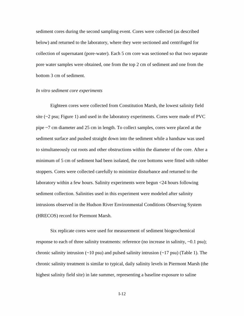
sediment cores during the second sampling event. Cores were collected (as described

below) and returned to the laboratory, where they were sectioned and centrifuged for

collection of supernatant (pore-water). Each 5 cm core was sectioned so that two separate

pore water samples were obtained, one from the top 2 cm of sediment and one from the

bottom 3 cm of sediment.

In vitro sediment core experiments

Eighteen cores were collected from Constitution Marsh, the lowest salinity field

site (~2 psu; Figure 1) and used in the laboratory experiments. Cores were made of PVC

pipe ~7 cm diameter and 25 cm in length. To collect samples, cores were placed at the

sediment surface and pushed straight down into the sediment while a handsaw was used

to simultaneously cut roots and other obstructions within the diameter of the core. After a

minimum of 5 cm of sediment had been isolated, the core bottoms were fitted with rubber

stoppers. Cores were collected carefully to minimize disturbance and returned to the

laboratory within a few hours. Salinity experiments were begun <24 hours following

sediment collection. Salinities used in this experiment were modeled after salinity

intrusions observed in the Hudson River Environmental Conditions Observing System

(HRECOS) record for Piermont Marsh.

Six replicate cores were used for measurement of sediment biogeochemical

response to each of three salinity treatments: reference (no increase in salinity, ~0.1 psu);

chronic salinity intrusion (~10 psu) and pulsed salinity intrusion (~17 psu) (Table 1). The

chronic salinity treatment is similar to typical, daily salinity levels in Piermont Marsh (the

highest salinity field site) in late summer, representing a baseline exposure to saline

I-12

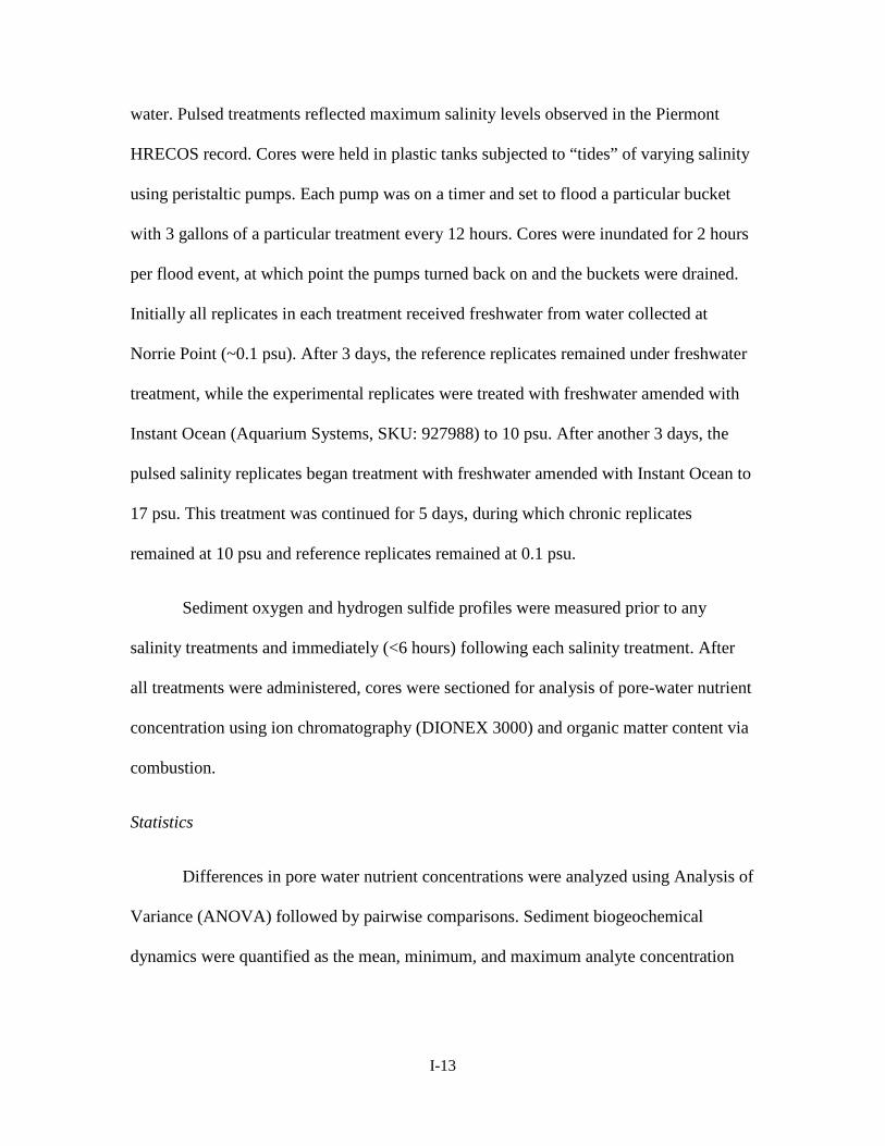
water. Pulsed treatments reflected maximum salinity levels observed in the Piermont

HRECOS record. Cores were held in plastic tanks subjected to “tides” of varying salinity

using peristaltic pumps. Each pump was on a timer and set to flood a particular bucket

with 3 gallons of a particular treatment every 12 hours. Cores were inundated for 2 hours

per flood event, at which point the pumps turned back on and the buckets were drained.

Initially all replicates in each treatment received freshwater from water collected at

Norrie Point (~0.1 psu). After 3 days, the reference replicates remained under freshwater

treatment, while the experimental replicates were treated with freshwater amended with

Instant Ocean (Aquarium Systems, SKU: 927988) to 10 psu. After another 3 days, the

pulsed salinity replicates began treatment with freshwater amended with Instant Ocean to

17 psu. This treatment was continued for 5 days, during which chronic replicates

remained at 10 psu and reference replicates remained at 0.1 psu.

Sediment oxygen and hydrogen sulfide profiles were measured prior to any

salinity treatments and immediately (<6 hours) following each salinity treatment. After

all treatments were administered, cores were sectioned for analysis of pore-water nutrient

concentration using ion chromatography (DIONEX 3000) and organic matter content via

combustion.

Statistics

Differences in pore water nutrient concentrations were analyzed using Analysis of

Variance (ANOVA) followed by pairwise comparisons. Sediment biogeochemical

dynamics were quantified as the mean, minimum, and maximum analyte concentration

I-13

for each sediment profile and also compared using ANOVA. All statistical analyses were

conducted using SAS Statistical Software.

Date Time Freshwater Salinity (ppt)

Chronic Salinity (ppt)

Pulsed Salinity (ppt)

7/21/2011 20:00 0.1 0.1 0.1 7/22/2011 08:00 0.1 0.1 0.1 7/22/2011 20:00 0.1 0.1 0.1 7/23/2011 08:00 0.1 0.1 0.1 7/23/2011 20:00 0.1 0.1 0.1 7/24/2011 08:00 0.1 0.1 0.1 7/24/2011 20:00 0.1 10.1 10.0 7/25/2011 08:00 0.1 10.3 9.9 7/25/2011 20:00 0.1 10.1 10.1 7/26/2011 08:00 0.1 10.0 10.0 7/26/2011 20:00 0.1 10.4 10.4 7/27/2011 08:00 0.1 10.5 10.5 7/27/2011 20:00 0.1 10.4 17.3 7/28/2011 08:00 0.1 10.5 17.2 7/28/2011 20:00 0.1 10.5 17.1 7/29/2011 08:00 0.1 10.0 17.5 7/29/2011 20:00 0.1 10.0 17.2 7/30/2011 08:00 0.1 9.7 17.7 7/30/2011 20:00 0.1 10.0 17.3 7/31/2011 08:00 0.1 10.4 17.2 7/31/2011 20:00 0.1 10.5 17.3 8/1/2011 08:00 0.1 10.0 17.1

Table 1. Salinity treatments applied during in vitro core experiments. Treatments were administered every 12 hours (8:00 and 20:00) for 11 days. Salinity changes occurred on 24 July 2011 for the chronic and pulsed treatments and again on 27 July 2011 for the pulsed treatments only. The reference treatments (freshwater) remained at a constant salinity throughout the experiment.

I-14

RESULTS

In situ descriptive sampling: Pore-water chemistry

Chloride concentrations in August were significantly higher in Piermont Marsh, the

southernmost site, relative to other sites, with concentrations averaging 6000 mg Cl-/L in

sediments (Figure 2; p<0.01). The three northernmost sites had average pore water

chloride concentrations ranging from 1900 mg Cl-/L in Con Hook Marsh to 2600 mg Cl-

/L in both Constitution and Iona Marshes (Figure 2).

Sulfate concentrations followed this trend, with Piermont Marsh having higher

concentrations (mean = 717 mg SO43-/L; p<0.01). Constitution Marsh had mean sulfate

SiteConstitution ConHook Iona Piermont

sedi

men

t chl

orid

e (m

g C

l- /L)

0

2000

4000

6000

8000

10000

12000

14000

bottomtop

Increasing Salinity

Figure 2. Sediment chloride concentrations in field study sites along salinity axis. Sites are arranged from left to right in order of increasing surface water salinity. Stacked bars are mean chloride concentrations (mg Cl-/L) in the top 2 cm and bottom 3 cm of 5 cm sediment cores extracted from each site. N = 6 for each bar.

I-15

concentrations of 320 mg SO43-/L, while Iona and Con Hook Marshes had pore-water

sulfate concentrations of 248 mg SO43-/L and 143 mg SO4

3-/L, respectively (Figure 3).

Nitrate concentrations were also highest in Piermont Marsh, which had maximum

concentrations of 12 mg NO3--N/L. In Constitution and Iona Marshes, sediment pore-

water nitrate concentrations were 4.5 mg NO3--N/L and Con Hook Marsh had mean

concentrations of 2 mg NO3--N /L (Figure 4). In contrast, Constitution, Con Hook, and

Piermont Marsh sediments all had lower sulfide concentrations, ranging from 0.12 to

0.18 mg H2S/L, whereas Iona Marsh had a significantly higher H2S concentration (mean

= 0.5 mg H2S/L; p<0.01; Figure 5).


sedi

men

t sul

fate

(mg

SO

43-/L

)

0

200

400

600

800

1000

1200

1400

1600

bottomtop

Increasing Salinity

Figure 3. Sediment sulfate concentrations in field study sites along salinity axis. Sites are arranged from left to right in order of increasing salinity. Stacked bars are mean sulfate concentrations (mg SO4

3-/L) in the top 2 cm and bottom 3 cm of 5 cm cores extracted from each site. N = 6 for each bar.

I-16


sedi

men

t nitr

ate

(mg

NO

3-N

/L)

0

5

10

15

20

25

30

bottomtop

Increasing Salinity

Figure 4. Sediment nitrate concentrations in field study sites along salinity axis. Sites are arranged from left to right in order of increasing salinity. Stacked bars are mean nitrate concentrations (mg NO3

--N/L) in the top 2 cm and bottom 3 cm of 5 cm cores extracted from each site. N = 6 for each bar.


sedi

men

t sul

fide

(mg

H2S

/L)

0.0

0.2

0.4

0.6

0.8

1.0

1.2

bottomtop

Increasing Salinity

Figure 5. Sediment sulfide concentrations in field study sites along salinity axis. Sites are arranged from left to right in order of increasing salinity. Stacked bars are mean sulfide concentration (mg H2S/L) in the top 2 cm and bottom 3 cm of 5 cm cores extracted from each site. N = 6 for each bar.

I-17

In situ descriptive sampling: Sediment oxygen dynamics

Maximum and mean oxygen concentrations had distinct temporal and spatial

variation across the study sites. Although maximum oxygen concentrations did not vary

among sites within a sampling period (p>0.1), maximum oxygen concentrations were

significantly different between the June and August sampling events (p<0.01). Mean

maximum oxygen concentration in June was 12 mg/L for all four sites, whereas, in

August the mean maximum oxygen concentration was 8 mg/L across sites (Figure 6).

Mean oxygen concentrations exhibited spatial, north to south, variation with higher mean

sediment concentrations at the northernmost site, Constitution Marsh (mean = 4 mg

O2/L; p<0.01). Con Hook and Piermont had the lowest mean oxygen concentrations in

August both being <3 mg O2/L. During the August sampling event, mean oxygen

concentrations in sediments dropped below 2 mg O2/L at all sites except Constitution

Marsh. Piermont Marsh exhibited the lowest mean O2 levels during both sampling events

(Figure 7).

I-18

Site

Const ConHook Iona Piermont

Max

imum

O2

(mg/

L)

0

2

4

6

8

10

12

14

AugustJune

Increasing Salinity

Figure 6. Variation in maximum oxygen concentrations of wetland sediments at study sites in June and August 2011. Sites are arranged from left to right in order of increasing salinity. N = 3 for each bar.

Constitution Con Hook Iona Piermont

SIte

Site

Const ConHook Iona Piermont

Mea

n O

2 (m

g/L)

0

1

2

3

4

5AugustJune

Increasing Salinity

Figure 7. Variation in mean oxygen concentrations of wetland sediments at study sites in June and August 2011. Sites are arranged from left to right in order of increasing salinity. N = 3 for each bar.


Site

I-19

In situ descriptive sampling: Sediment sulfide dynamics

In August, mean sulfide concentrations were highest in Con Hook and Iona

Marshes, >10 mg H2S/L in sediments. Piermont Marsh had mean sediment sulfide

concentration of 9 mg/L while Constitution Marsh had the lowest mean sulfide

concentrations of 5 mg/L (Figure 8). The maximum sulfide concentration in Con Hook

Marsh was 60 mg H2S /L. Iona Marsh had maximum sulfide concentrations of 20 mg

H2S /L; whereas, at Constitution and Piermont maximum sulfide concentrations were

<20 mg H2S/L (Figure 9). Piermont Marsh was the only site where sulfide concentrations

were always above detection (≥4 mg/L). Constitution, Iona, and Con Hook Marshes all

had minimum sediment sulfide concentrations below the detection limit of 0.01 mg

H2S/L (Figure 10).

SiteConst ConHook Iona Piermont

Mea

n S

edim

ent H

2S (m

g/L)

0

5

10

15

20

25

30

Increasing Salinity

Figure 8. Mean sediment sulfide concentrations of wetland sediments at study sites in August 2011. Sites are arranged from left to right in order of increasing salinity. N = 3 for each bar.


Site

I-20

SiteConst ConHook Iona Piermont

Max

imum

Sed

imen

t H2S

(mg/

L)

0

20

40

60

80

100

120Increasing Salinity

Figure 9. Maximum sediment sulfide concentrations of wetland sediments at study sites. Sites are arranged from left to right in order of increasing salinity. N = 3 for each bar.


Sites

Site

Const ConHook Iona Piermont Spiked

Min

imum

H2S

(mg/

L)

02468

1012141618

Increasing Salinity

Figure 10. Minimum sediment sulfide concentrations in sediment of pulsed salinity cores in the laboratory experiment and field study sites. N = 3 for each bar.

Constitution Con Hook Iona Piermont Spiked

Sites

I-21


Water chemistry analysis revealed average chloride concentrations of 5300 mg Cl-

/L in sediments undergoing pulsed treatments. Sulfate concentrations averaged 400 mg

SO43-/L and nitrate was found at average concentrations of 16 mg NO3--N/L in these

sediments. Mean maximum oxygen concentration was 6 mg O2/L in these cores and

mean oxygen concentrations were 1 mg O2/L.

Mean sediment sulfide concentrations in pulsed salinity cores ranged from 10-15

mg H2S/L. A maximum sulfide concentration of 20 mg H2S/L and a minimum

concentration of around 4 mg H2S/L were also recorded in these experimental cores

(Figure 10).

DISCUSSION

Pore-water analysis

Analysis of pore-water chemistry illustrated the contrast in chemical

concentrations between the northern end of the salinity gradient and the southern end. In

many cases, such as with chloride, sulfate, and nitrate, the three northernmost sites (Iona,

Con Hook, and Constitution) had similar pore-water concentrations, whereas Piermont

Marsh had significantly different concentrations. The higher chloride and sulfate

concentrations in Piermont were expected, as these are the two major ions in salt water

and Piermont Marsh contains the highest salinity waters across the study sites. However,

Piermont sediments also had higher nitrate concentrations, which would not be directly

I-22

influenced by saltwater but may be the result of changes in microbial activity (Magalhães

et al. 1980). Similarly, pulsed salinity sediment cores exhibited concentrations of

chloride, sulfate and nitrate that were higher than the three northernmost sites and

comparable to Piermont marsh. Chloride concentrations were higher in Piermont, but

sulfate was higher in pulsed cores. Some variation in chemical composition would be

expected between artificial seawater and seawater from a natural system. Higher nitrate

levels in the higher salinity pulsed core sediments further suggest a relationship between

salinity and nitrate concentrations.

The lack of variation in pore-water chemistry among the three northernmost sites

(Constitution, Iona, and Con Hook) may be explained by the proximity of these sites to

one another (Figure 1). At a distance of nearly 10 miles downstream, Piermont Marsh is

by far the southernmost site of the four, whereas Constitution, Con Hook, and Iona

Marshes all exist within ~3 miles of one another at the extreme north end of the sampling

region. This likely explains the lack of statistical differences between these sites in terms

of chloride, sulfate, and nitrate concentrations.

Sediment sulfide concentrations did not follow the trend of higher concentrations

at Constitution. Rather, significantly higher sediment sulfide concentrations were

measured at Iona Marsh relative to other sites, which was not expected. One possible

explanation is that Iona Marsh may retain more water than other sites. As a result, it may

be that less sulfide is lost from these sediments, allowing for an accumulation over time

and accounting for these higher concentrations.

I-23

In situ descriptive sampling: Sediment oxygen dynamics

The oxygen dynamics reported in the field data are what would be expected, both

in terms of maximum and mean O2 concentrations. Maximum oxygen concentrations

were lower at all sites in the August sampling relative to the June sampling. These data

suggest that as the summer progressed, either increased temperatures and/or sediment

microbial respiration depleted available oxygen yielding lower oxygen concentrations.

In situ descriptive sampling: Sediment sulfide dynamics

Neither mean nor maximum sediment H2S concentrations varied along the

anticipated salinity gradient. This lack of variation may be due to all sites having similar

sediment microbial communities and potential for reducing sulfate to hydrogen sulfide.

However, because Piermont Marsh was the only site in which sulfide was always present,

regular exposure to higher salinity waters may result in greater retention of sulfide by

wetland sediments.


Cores undergoing pulsed salinity treatments exhibited similar biogeochemical

activity to Piermont Marsh (highest salinity) sediments. Specifically, maximum and mean

oxygen concentrations were similar; however, pulsed salinity cores became anoxic at

greater sediment depths relative to Piermont Marsh sediment (Figure 11). This may have

been an experimental artifact, as oxygen may not have diffused as well through

I-24

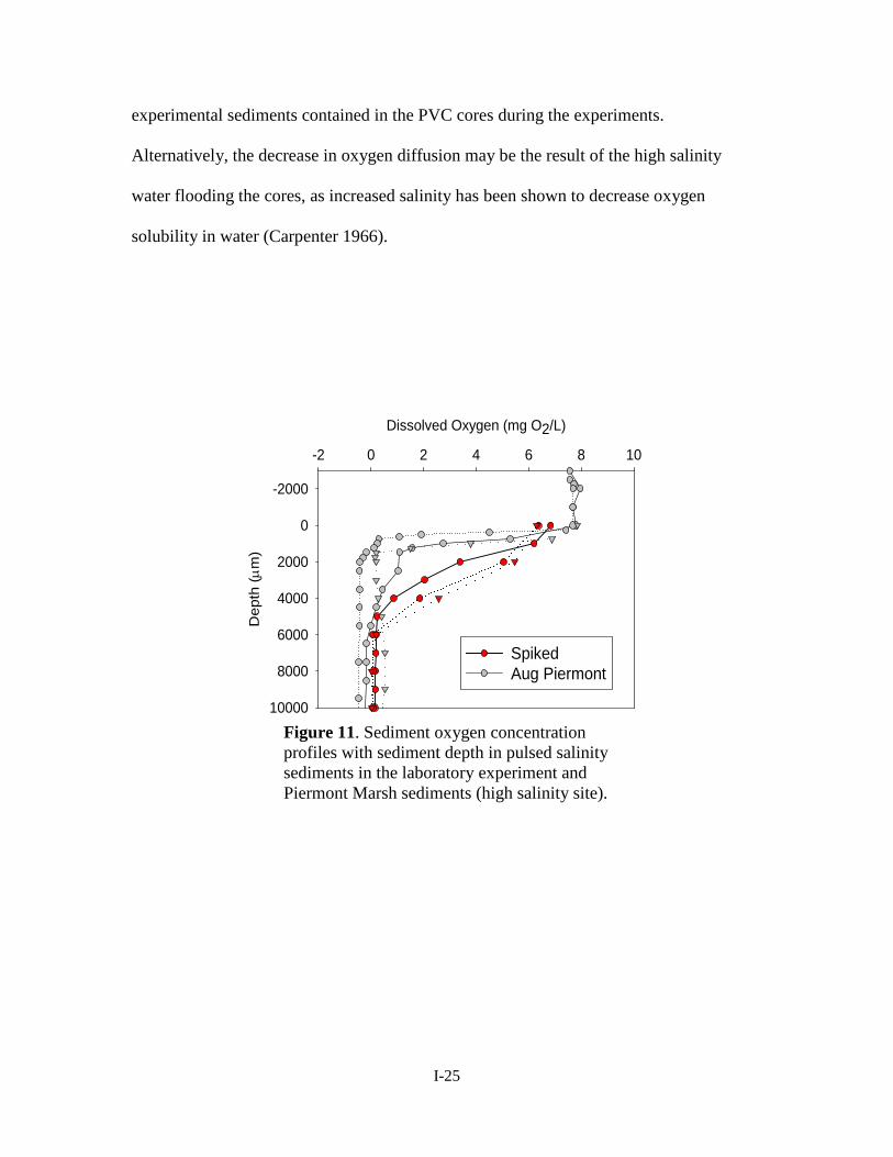
experimental sediments contained in the PVC cores during the experiments.

Alternatively, the decrease in oxygen diffusion may be the result of the high salinity

water flooding the cores, as increased salinity has been shown to decrease oxygen

solubility in water (Carpenter 1966).

Dissolved Oxygen (mg O2/L)

-2 0 2 4 6 8 10

Dep

th (µ

m)

-2000

0

2000

4000

6000

8000

10000

SpikedAug Piermont

Figure 11. Sediment oxygen concentration profiles with sediment depth in pulsed salinity sediments in the laboratory experiment and Piermont Marsh sediments (high salinity site).

I-25

Sediment sulfide concentrations were also similar between Piermont Marsh and

pulsed salinity cores. In addition to comparable mean and maximum sediment sulfide

concentrations, these two sediments were the only instances in which sulfide was never

completely depleted (Figure 10). Further, sulfide levels in these sediments mimic those

reported by previous research. DeLaune et al. (1982) reported sulfide concentrations of 6

mg H2S/L in brackish water sediments (0.5-18 psu) and 20 mgH2S/L in sediments

regularly exposed to seawater (18-30 psu). Additionally, Baldwin and Mendelssohn

(1998) have shown average hydrogen sulfide concentrations of 6.7 mg H2S/L

corresponding to a salinity of 6 psu. Salinities at Piermont Marsh rarely exceeded these

levels, as this was an unusually wet year in regard to rainfall.

Conclusions

These data present potential implications associated with higher salinity waters in tidal

freshwater wetland sediments as a result of increases in both nitrate and sulfide

concentrations. Exposure to occasional salinity increases and the resultant sulfate

reduction is not uncommon throughout the brackish region of the Hudson River estuary;

however, consistent exposure to high salinities, as seen in Piermont Marsh, may lead to a

greater retention of sulfide, most likely as a result of more constant sulfate reduction.

Further, resulting higher concentrations of sulfide will put these wetlands at risk for

increased nitrogen retention through a favoring of dissimilatory nitrate reduction to

ammonia over denitrification. Also, if the increased sulfate reduction that typically results

in high sulfide concentrations is an indication of greater mineralization of organic matter,

I-26

steady rates of accretion may not be maintained in these wetlands. Furthermore, the

continued outpacing of accretion by mineralization may result in the loss of tidally

influenced freshwater wetlands of the Hudson River to rising sea levels.

I-27

ACKNOWLEDGEMENTS

I thank the Tibor T. Polgar fellowship program and the Hudson River Foundation for funding; the Cary Institute of Ecosystem Studies for housing assistance; and David Yozzo, Helena Andreyko, Sarah Fernald, David Fischer and Oscar Azucena for assistance.

I-28

REFERENCES

Arrigoni, A., S. Findlay, D. Fischer, and K. Tockner. 2008. Predicting carbon and nutrient transformations in tidal freshwater wetlands of the Hudson River. Ecosystems 11:790-802.

Baldwin, A.H. and I.A. Mendelssohn. 1998. Effects of salinity and water level on coastal marshes: an experimental test of disturbance as a catalyst for vegetation change. Aquatic Botany 61:255-268.

Barbier, E.B., E.W. Koch, B.R. Silliman, S.D. Hacker, E. Wolanski, J. Primavera, E.F. Granek, S. Polasky, S. Aswani, L.A. Cramer, D.M. Stoms, C.J. Kennedy, D. Bael, C.V. Kappel, G.M.E. Perillo, and D.J. Reed. 2008. Coastal Ecosystem-Based Management with Nonlinear Ecological Functions and Values. Science 319:321-323.

Brunet, R.C., and L.J. Garcia-Gil. 1996. Sulfide-induced dissimilatory nitrate reduction to ammonia in anaerobic freshwater sediments. FEMS Microbial Ecology 21:131-138.

Cai, W., W.J. Wiebe,, Y. Wang, and J.E. Sheldon. 2000. Intertidal marsh as a source of dissolved inorganic carbon and a sink of NO3

- in the Satilla River-estuarine complex in southeastern U.S. Limnology and Oceanography 45:1743-1752.

Capone, D.G. and R.P. Kiene. 1988. Comparison of microbial dynamics in marine and

freshwater sediments – contrasts in anaerobic carbon catabolism. Limnology and Oceanography 33:725-749.

Carpenter, J.H. 1966. New measurements of oxygen solubility in pure and natural water.

Limnology and Oceanography 12:264-277. DeLaune, R.D., C.J. Smith., and W.H. Patrick. 1982. Methane release from Gulf Coast

wetlands. Tellus B 35B:8-15. Giblin, A.E., N.B. Weston, G.T. Banta, J. Tucker, and C.S. Hopkinson. 2010. The

effects of salinity on nitrogen losses from an oligohaline estuarine sediment. Estuaries and Coasts 33:1054-1068.

Greene, S.E. 2005. Nutrient removal by tidal fresh and oligohaline marshes in a

Chesapeake Bay tributary. MS Thesis. University of Maryland Solomons, MD, 149pp.

Gribsholt, B., H.T.S. Boschker, E. Struyf, M. Andersson, A. Tramper, L. De Brabandere,

S. van Damme, N. Brion, P. Meire, F. Dehairs, J.J. Middelburg, and C.H.R. Heip. 2005. Nitrogen processing in a tidal freshwater marsh: A whole-ecosystem 15N labeling study. Limnology and Oceanography. 50:1945-1959.

I-29

Hamilton, P. 1990. Modelling salinity and circulation for the Columbia River Estuary. Progress in Oceanography 25:113-156.

Jeroschewski, P., C. Steuckart, and M. Kahl. 1996. An amperometric microsensor for the

determination of H2S in aquatic environments. Analytical Chemistry 68:4351-4357.

Joye, S.B. and J.T. Holibaugh. 1995. Influence of sulfide inhibition of nitrification on

nitrogen regeneration in sediments. Science 270:623-625. Kelley, C.A., C.S. Martens, and J.P. Chanton. 1990. Variations in sedimentary carbon

remineralization rates in the White Oak River estuary, North Carolina. Limnology and Oceanography 35:372-383.

Kemp, M. and W. Dodds. 2001. Centimeter-scale patterns in dissolved oxygen and

nitrification rates in a prairie stream. Journal of the North American Benthological Society 20:347-357.

Kiviat, E., S.E.G. Findlay, S., and W. C. Nieder. 2006. Tidal Wetlands of the Hudson

River Estuary. pp. 279-310. in: J.S. Levinton and J.R. Waldman (Eds). The Hudson River Estuary. New York. Cambridge University Press.

Knowles, N. 2002. Natural and management influences on freshwater inflows and

salinity in the San Francisco Estuary at monthly to interannual scales. Water Resources Research 38:1289-1299.

Magalhães, C.M., S.B. Joye,, R.M. Moreira, W.J. Wiebe, and A.A. Bordalo. 1980. Effect

of salinity and inorganic nitrogen concentrations on nitrification and denitrification rates in intertidal sediments and rocky biofilms of the Douro River estuary, Portugal. Water Research 39:1783-1794.

Megonigal, J.P. and S.C. Neubauer. 2009. Biogeochemistry of tidal freshwater wetlands.

pp. 535-562. in: G.M.E. Perillo, E. Wolanski, D.R. Cahoon, and M.M. Brinson (Eds). Coastal Wetlands: An Integrated Ecosystem Approach. Elsevier.

Milly, P.C.D., K.A. Dunne, and A.V. Vecchia. 2005. Global pattern of trends in

streamflow and water availability in a changing climate. Nature 438:347-350. Mitsch, W.J. and J.G. Gosselink. 1993.Wetlands, 2nd Ed. New York. John Wiley &

Sons, p. 722. Morris, J.T., P.V. Sundareshwar, C.T. Nietch, B. Kjerfve, and D.R. Cahoon. 2002.

Responses of coastal wetlands to rising sea level. Ecology 83:2869-2877.

I-30

Neubauer, S.C., K. Givier, S.K. Valentive, and J.P. Megonigal. 2005. Seasonal patterns and plant-mediated controls of subsurface wetland biogeochemistry. Ecology 86:3334-3344.

Redfield, A.C. 1965. Ontogeny of a salt marsh estuary. Science 147: 50-55. Revsbech, N. and B. Jørgensen. 1986. Microelectrodes: their use in microbial ecology.

Advances in Microbial Ecology 9:293-352. Seitzinger, S.P. 1988. Denitrification in freshwater and coastal marine ecosystems:

Ecological and geochemical significance. Limnology and Oceanography 33:702-724.

Seitzinger, S.P. and R.W. Sanders. 2002. Bioavailability of DON from natural and

anthropogenic sources to estuarine plankton. Limnology and Oceanography 47:353-366.

Smith, T.M., T.C. Peterson, J.H. Lawrimore, and R.W. Reynolds. 2005. New surface

temperature analyses for climate monitoring. Geophysical Research Letters 32:L14712, 4 pp.

Weston, N.B., M.A. Vile, S.C. Nebauer, and D.J. Velinsky. 2010. Accelerated microbial

organic matter mineralization following salt-water intrusion into tidal freshwater marsh soils. Biogeochemistry 102:135-151.

I-31

TRACING COMBINED SEWAGE OVERFLOW DISCHARGE WITH QUATERNARY AMMONIUM COMPOUNDS


Patrick C. Fitzgerald

Polgar Fellow

School of Marine and Atmospheric Sciences Stony Brook University Stony Brook, NY 11794

Project Adviser:

Bruce J. Brownawell School of Marine and Atmospheric Sciences

Stony Brook University Stony Brook, NY 11794

Fitzgerald, P.C. and B.J. Brownawell. 2012. Tracing Combined Sewage Overflow Plumes with Quaternary Ammonium Compounds. Section II: 1-31 pp. In D.J. Yozzo, S.H. Fernald, and H. Andreyko (eds.), Final Reports of the Tibor T. Polgar Fellowship Program, 2011. Hudson River Foundation.

II-1

ABSTRACT

Quaternary ammonium compounds are a novel class of chemical tracers for

sewage-derived contaminants. In this study, it is hypothesized that these tracers make it

possible to distinguish between treated and untreated sewage sources in estuarine surface

waters. Sites around the Lower Hudson Basin were sampled from May 2011 through

October 2011, with particular emphasis on the East River, Newtown Creek, and Gowanus

Canal. Corresponding measurements of fecal indicator bacteria were made by another

research group at these sites. Limited sampling was also conducted in the Hudson River

along the Manhattan shoreline and at Piermont at the municipal sewage outfall. Samples

were also collected during the raw sewage discharge that resulted from a failure in the

North River Wastewater Treatment Plant in July. Samples were analyzed using high

performance liquid chromatography with a time-of-flight mass spectrometer. Most

samples were analyzed for particulate phase tracers only.

The first successful measurements of quaternary ammonium compounds (QACs)

were made in estuarine surface waters of the U.S. The composition of these sewage-

specific tracers was found to vary with the amount of rainfall on the previous day, more

closely representing that of untreated sewage after large rainfalls. This finding lends

credence to the idea that combined sewage overflow is one of the largest sources of

contaminants to the water column in New York’s industrial canals. The total

concentration of QACs also exhibited a weak correlation with the abundance of fecal

indicator bacteria. A pronounced compositional change was also observed during the

North River Plant’s failure. Although the ability to discriminate between treated and

untreated sewage sources was not as great as expected, further specificity may be

possible by measuring tracers in the dissolved phase.

II-2

TABLE OF CONTENTS

Abstract……………………………………………….………………………… II-2

Table of Contents……………………………………………………………….. II-3

Lists of Figures and Tables……………………………………………………… II-4

Introduction……………………………………………………………………… II-5

Methods………………………………………………………………………….. II-13

Sampling Sites…………………………………………………………… II-13

Procedure…………………………………………………………………. II-16

Results……………………………………………………………………………. II-17

Discussion………………………………………………………………………… II-25

Acknowledgments………………………………………………………………... II-29

Literature Cited…………………………………………………………………… II-30

II-3

LISTS OF FIGURES AND TABLES

List of Figures

Figure 1. Three environmentally significant series of QACs……………… II-9

Figure 2. Maps of sampling locations……………………………………… II-15

Figure 3. Ranges of QAC concentrations at four sites…………………….. II-20

Figure 4. Ranges of QAC compositions at four sites………………………. II-21

Figure 5. Relationship between prior day rainfall and QAC composition… II-21

Figure 6. Relationship between behentrimonium and FIB concentrations… II-22

Figure 7. Relationship between FIB concentrations and prior day rainfall…. II-22

Figure 8. August QAC concentrations at Piermont……………………….... II-23

Figure 9. Particulate vs. dissolved partitioning at Piermont……………….. II-23

Figure 10. Changing conditions with distance from raw sewage discharge… II-24

Figure 11. Comparison of Compositions Across 10 kinds of sample………. II-27

List of Tables

Table 1. Grouping of analytes into more labile and less labile fractions….… II-10

Table 2. Sampling sites and dates………………………………………..….. II-16

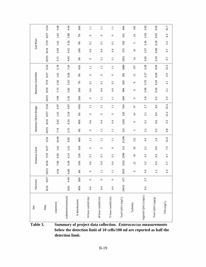
Table 3. Summary of project data collection………………….……………. II-19

II-4

INTRODUCTION

Water quality in the Lower Hudson Basin has improved significantly over the last

few decades, thanks in part to investments in improved waste water treatment, such as the

1986 construction of the North River treatment plant in Manhattan. This improvement

has led to a renewed interest in recreational use of the river for activities such as

swimming and fishing. However, the Hudson still receives a tremendous amount of

sewage (not all of which is well-treated) and water quality issues persist. Combined

sewage overflow (CSO) systems, which integrate stormwater and wastewater, may cause

waste water treatment plants (WWTPs) to become overloaded during a precipitation

event, and force them to discharge poorly-treated sewage into the Hudson. These

systems are a significant source of pathogens, chemical contaminants, nutrients, and

debris to the estuary. It is also possible that the spread of untreated sewage in the

environment could promote the spread of antibiotic resistance (McLellan et al. 2007).

Sewage-derived pathogens are among the most serious threats to swimmers and shellfish

consumers (Donovan et al. 2008), and vary spatially and temporally in abundance

(NYCDEP 2010). The inconsistent presence of harmful microorganisms presents a

challenge to estuary managers seeking to issue safety advisories to the public. Although

CSOs are an important source of pathogens, these organisms also enter the water column

from other sources as well, and the relative contributions of these sources are poorly

understood (Simpson et al. 2010). Currently employed water quality analyses in the

Hudson do not impart a high degree of source-specificity, making it difficult to accurately

assess the environmental impact of New York’s aging CSO system. In this study, a novel

class of sewage-derived chemical tracers is explored: quaternary ammonium compounds

II-5

(QACs). These information-rich tracers have the potential to assess contamination

sources with high specificity.

The metric currently used to estimate the threat posed by pathogens in surface

waters is the abundance of fecal indicator bacteria (FIB). These organisms are not

necessarily pathogenic, but their abundance is thought to correlate with that of more

harmful sewage-derived pathogens (Wheeler et al. 2002). In the Lower Hudson Basin

and other estuaries, Enterococcus is the primary FIB, as it is ubiquitous in the guts of

endothermic organisms and can survive some time in salt water (Freis et al. 2008).

Enterococcus measurements are appealing because they can be done easily and cheaply

(after an initial investment in equipment). However, this technique does not provide

information regarding pathogen sources. More sophisticated molecular biological

techniques have been tested and are still developing (Simpson et al. 2010; Stoeckel and

Harwood 2007) to identify FIB by their original host organisms (humans, ducks, etc.).

While potentially powerful, the accuracy of molecular source-tracking is hindered by the

ever-fluctuating compositions of the gut flora found in animals, and because the

population of enteric bacteria in an animal’s digestive tract varies as a function of the

host’s health and diet (Simpson et al. 2010). Furthermore, identification of a host

organism is only one part of source trackdown, because pathogens from a single species

of host (notably humans) can still be introduced into the water column by a variety of

mechanisms.

Reduction of pathogen loading into the estuary is dependent on understanding

how pathogens enter the water column. CSO discharge is one of the most prominent

loading mechanisms, but high FIB abundances can still be measured at times during dry

II-6

spells or in areas of the Hudson Basin which are not proximate to a CSO outfall. Several

FIB sources have been identified, including:

• Undertreated sewage: This can be introduced to receiving waters through CSO

discharge, or as a result of mechanical failures in the wastewater treatment

process. Significant discharges of untreated sewage entered the Hudson as a

result of the fire at the North River WWTP in July 2011, and again in August

2011 when a waste pipe was damaged in Ossining, NY. Furthermore, illicit

discharges of wastewater can feed into storm drains, entering receiving waters

directly.

• Treated sewage: Although disinfection of wastewater removes most pathogenic

organisms, it is not always 100% effective. Particles can shelter some

microorganisms from disinfection, while organisms such as Giardia are resistant

to chlorination (Jarrol et al. 1981).

• Resuspended Sediments: Certain sewage-derived pathogens can persist in the

sediment for significant periods of time after settling out of the water column.

Resuspension of sediments by storms or ship wakes can then mix pathogens back

into the water column (Jeng et al. 2005) independent of CSO discharge.

• Surface runoff: Surfaces can be contaminated with bacteria from animal feces,

including pets, livestock, rodents, birds, and others. During rain events, this

contamination can be washed into storm drains, directly into estuaries (e.g.,

through streams), or into CSO systems—particularly on impervious surfaces in

urban areas with no riparian buffer zone.

II-7

• Groundwater: Leaking septic tanks and aging sewer lines can contaminate

groundwater with fecal organisms. Under the right conditions, pathogens can be

carried into the estuary by the flow of groundwater (Hagerdorn and Weisberg

2009).

Given the multiplicity of sources, it can be difficult to attribute high FIB abundances

in surface waters specifically to CSO. Chemical analyses which rely on the concentration

or presence/absence of a single tracer can be further confounded by the large amount of

dilution experienced by contaminants when sewage enters receiving waters. Tracers have

included compounds such as caffeine, silver ions, nitrogen isotopes, fluorescent

whitening agents (FWAs), pharmaceuticals, and others (Haack et al. 2009; Hagerdorn

and Weisberg 2009; Simpson et al. 2010). Although these tracers can provide useful

information about the extent of anthropogenic contamination in a waterway, they are

often limited by factors including natural background concentrations, or dilution to

concentrations below detection limits. Furthermore, as individual compounds, their

presence alone cannot distinguish between treated and untreated sewage. A valuable

analysis to complement existing tracers and generate more layers of information involves

the use of quaternary ammonium compounds (QACs), which possess unique properties as

tracers (Li and Brownawell 2009; Li and Brownawell 2010) but are to-date understudied

in surface waters.

QACs are a class of permanently charged organic cations, commonly used as

disinfectants, surfactants, and anti-static agents in a variety of personal care products,

cleaning products, and industrial processes. They all consist of one nitrogen atom with a

positive charge, bonded to four hydrocarbon groups. With large, hydrophobic carbon

II-8

chains and a positive charge, QACs are highly particle-reactive in estuarine water, a

property that increases in QACs with higher molecular weights. Due to widespread use,

QACs are ubiquitous in sewage and abundant in sewage-impacted waters. Many of these

compounds are not thoroughly degraded by microbial action in waste water treatment

(particularly the largest, least bioavailable compounds). It has recently been shown that

QACs are in many cases the most abundant organic contaminants measured in estuarine

sediments around New York Harbor (Li and Brownawell 2009; Li and Brownawell 2010;

Li 2009; Lara-Martin et al. 2010), and other sewage impacted estuaries including Long

Island Sound and Hempstead Harbor (unpublished) because of high loading rates and

significant persistence. Three homologous series of QACs have been identified as

environmental contaminants, including alkyltrimethyl ammonium chlorides (ATMAC),

benzalkonium chlorides (BAC), and dialkyldimethylammonium chlorides (DADMAC)

(Figure 1).

Figure 1. Three environmentally significant series of QACs: ATMAC, BAC, and DADMAC.

II-9

The large number of QACs which can be found in the Hudson River Estuary

contributes to their potential as a set of highly source-specific tracers. Because they vary

greatly in size, these compounds span a range of solubilities and bioavailabilities, and

thus exhibit different behavior in waste water treatment and the environment. The more

labile QACs (such as BACs, many of which can be used as algaecides at high

concentration) are efficiently metabolized by heterotrophic bacteria, particularly in the

sewage-acclimated microbial communities of WWTPs, and to some extent in waste-

receiving waters. There is a continuum of degradation in wastewater treatment plants as

a function of the alkyl chain length of QACs (Clara et al. 2007), with longer chain length

DADMACs (Figure 1) found to be essentially inert, and recent findings suggest that

many QACs are well-preserved once associated with estuarine sediments (Li and

Brownawell 2010; Lara-Martin et al. 2010). Thus, in poorly treated sewage, the fraction

of total QACs from the more labile group is higher, and in treated sewage, the labile

fraction is markedly diminished. This has been observed in sediments proximate to CSO

discharges (Li and Brownawell 2010), and it was proposed here that such distinctions can

be used to discriminate between treated and untreated sewage sources to receiving waters

by measuring the environmental concentrations of the compounds, and dividing the

aggregate concentration of “labile” compounds by the total QAC concentration. The

compounds are grouped as follows:

More labile QACs Less labile QACs ATMAC 16 BAC 16 ATMAC 18 DADMAC 16:16 BAC 12 DADMAC 8:10 BAC 18 DADMAC 16:18 BAC 14 DADMAC 10:10 DADMAC 14:14 DADMAC 18:18

DADMAC 14:16

Table 1. Grouping of analytes into more labile and less labile fractions.

II-10

This list does not include all analytes measured in the present study, in order to allow

direct comparison with harbor-wide sediment data reported by Li and Brownawell

(2010). Several compounds were added to the list of analytes since sediment data were

collected. Notably, ATMAC 22 (a common additive in personal care products,

commonly known as behentrimonium chloride) has since been discovered as one of the

most persistent QACs in New York Harbor (Lara-Martin et al. 2010). Another new

analyte, ATMAC 12, is much more soluble, is detected at high levels in the influent of

local WWTPs (unpublished data) and was anticipated to be present at much higher levels

in untreated sewage compared to biologically treated effluents from WWTPs.

A second piece of information lies in the partitioning of QACs between the

particulate and aqueous phases. In receiving waters, sewage becomes highly diluted, and

this dilution causes a portion of the QACs sorbed to particles to dissociate and enter the

aqueous phase. In the aqueous phase, they are more vulnerable to biodegradation and so

are less persistent. Accordingly, surface water which has received recent sewage

discharge (treated or otherwise) should contain a higher dissolved fraction of the more

soluble (“labile”) QACs, relative to water which has not experienced sewage discharge

for a period of several days. This difference should be observable in the environment by

filtering water samples and analyzing the particles and filtrate separately. Furthermore,

resuspended sediment should have a QAC pattern similar to that of “old” sewage

discharge, because the sediment in heavily sewage-impacted areas acquires most of its

QAC content from past discharge as it settles to the bottom.

Other sources of estuarine pathogens are not significant sources of QACs. As

very particle-reactive cations, QACs do not travel though the water table, as in some

II-11

cases pathogens and some nutrients can. For tracking groundwater contamination,

soluble tracers such as stable pharmaceuticals (e.g., carbamezapine and

sulfamethoxazole), FWAs and potentially caffeine may be useful tools if dilution is not

too great, as they can travel through groundwater (Swartz et al. 2006; Hagerdorn and

Weisberg 2009). However, the absence of QACs is itself a form of information. In rural

estuaries where groundwater is a suspected source of pathogens, it would be strong

evidence to find the presence of caffeine coupled with low levels of QACs, indicating

that pathogens assigned a human source are coming from the water table and not from

treatment plants. In the event that pathogens from animal feces are washed into the river

by runoff, again no QACs are expected to come from this pathway. Terrestrial surfaces

should not contain significant amounts of these compounds. Thus, while this study in the

highly sewage-impacted urban portion of the lower Hudson is most useful for

distinguishing between treated and poorly-treated sewage sources, QACs have potential

applications for additional source-specificity distinction between many possible pathogen

sources.

II-12

METHODS

Sampling sites

The majority of sampling was conducted by ship in collaboration with John Lipscomb

of Riverkeeper. These samples were taken in parallel with the FIB monitoring project

operated by Dr. Gregory O’Mullan of Queens College and Dr. Andrew Juhl of Lamont-

Doherty Earth Observatory. Shipside monitoring stations included:

• The East River (ER): This station was mid-channel near the mouth of Newtown

Creek. A tremendous amount of treated sewage is discharged into the East River

on a regular basis. Although it is very fast-flowing, the tidal reversal acts to

increase the residence time of contaminants in this section of the river.

• Newtown Creek—Dutchkills (DK): Once a natural creek, Newtown has long

served as an industrial canal. It receives CSO discharge and is also contaminated

with oil and other industrial contaminants, and is now a federal superfund site.

This station is at the intersection of Newtown and one of its tributaries, the

Dutchkills, not far from the mouth of the creek.

• Newtown Creek—Metropolitan Avenue Bridge (MB): This station is far in the

back of the canal, and thus is somewhat isolated from the East River, with

exchange of water between the two bodies occurring primarily as the result of

tidal mixing.

• Gowanus Canal (GC): This superfund site in Brooklyn is one of the most polluted

waterways in the country. In addition to CSO discharge, the canal is

contaminated by creosote and other industrially-derived pollutants. The sampling

station here is a short distance inland from the mouth of the canal.

II-13

• North River Plant (NR): This plant treats much of the sewage of upper Manhattan

and discharges it into the Hudson near 125th St. Sampling was conducted both at

the sewage outfall and at the nearby recreational pier.

• Dyckman St. Beach (DB): A small recreational pier is located on the Hudson at

the far north of Harlem. There is a CSO outfall pipe nearby.

• Piermont (PM): This site is north of New York City at a recreational pier in the

town of Piermont. A local WWTP discharges close to the pier; a limited number

of samples were collected at the outfall and just off the pier.

In addition to shipboard sampling, samples were taken from land in response to the

fire which disabled the North River Plant for three days in July 2011. Hundreds of

millions of gallons of undertreated sewage were redirected to a series of CSO outfalls

around Manhattan. Samples were taken near two of those outfalls on July 22nd, near the

end of the event. At 125th St., an outfall just south of the recreational pier was cordoned

off with a boom. Samples were taken from inside the boom as well as from the pier at

two distances away from the CSO. While sampling at these sites, the ebb tide was

observed to slacken to where the flow from the CSO towards the pier was very weak. At

Dyckman St. Beach, samples were taken from the pier proximate to the outfall, which

was also boomed off (Table 2).

II-14

(a) (b)

(c)

Figure 2. Maps of sampling locations: (a) Brooklyn sites including East River, Newtown-Dutchkills, Newtown-Metropolitan Ave. Bridge, and Gowanus Canal; (b) Stations along the Hudson River including North River Plant, Dyckman St. Beach, and Piermont; (c) Sites around North River Plant including WWTP outfall, CSO outfall, and two piers, 44m and 111m away from the CSO outfall, respectively.

II-15

Date Sites Prior Rainfall (inches) 24 hours 48 hours 72 hours

May 16th ER, DK, MB, GC 1.1 1.1 1.1 June 27th ER, DK, MB, GC, NR, PM 0 0 0 July 19th ER, DK, MB, GC 0.1 0.1 0.1 July 22nd NR, DB 0 0 0 August 16th ER, DK, MB, GC, NR, DB, PM 0.6 6.4 6.4 October 21st ER, DK, MB, GC 0 1.1 1.1 Table 2. Sampling sites and dates. Rainfall is given as a cumulative total over

three different intervals. Procedure

The analysis for surface water samples is based on the sediment analysis designed

by Li and Brownawell (2009), and further modified to include behentrimonium by Lara-

Martin et al. (2010). Surface water samples were collected in methanol-rinsed 1-L glass

bottles and fixed on-site as 1% formalin solutions to prevent further biodegradation of

analytes. In the laboratory, samples were filtered through pre-combusted Whatman GF/C

glass fiber filters under vacuum pressure to separate the particulate and dissolved phases.

Filters were then placed in vials and immersed in 10 ml of 10% HCl in methanol. To

extract analytes from the particulate phase, the filters were next sonicated at 60°C for one

hour in a water bath. After sonication, filters were centrifuged for 15 min at 2500 RPM,

and the solvent was decanted into a larger collection vial. This extraction process was

repeated two more times, and all three extracts were combined in the collection vial.

Extracts were evaporated to dryness with nitrogen gas and a 60°C water bath. For

purification, dry extracts were then resuspended in 2.5 ml of methanol and loaded onto a

weak anion-exchange resin (AG-1-X2 from BioRad). The analytes were then eluted using

12.5 ml of methanol.

II-16

Dissolved phase analytes were isolated from filtrate in select samples by solid

phase extraction, utilizing a method that is still under development, modified from the

procedure by Ferrer and Furlong (2001). Filtrate samples were converted to 25%

acetonitrile solutions and run through a Waters brand Oasis HLB cartridge under vacuum

pressure. Analytes were then eluted off the cartridge using 15 ml of 100% acetonitrile.

Both dissolved-phase and particulate extracts were analyzed with high performance

liquid chromatography using a time-of-flight mass spectrometer (HPLC-ToF-MS)

according to the procedure outlined by Li and Brownawell (2009; Li and Brownawell

2010).

RESULTS

QACs were successfully measured in surface water samples at all stations in the

Lower Hudson Basin (Table 3), although not all of the 19 targeted QACs were detected

in all samples. Samples exhibited a range of concentrations with a high of 31,200 ng/L,

and a low of 112 ng/L, both seen at Gowanus Canal (Figure 3), with a median of 652

ng/L. The composition of QACs ranged from 0% labile compounds to 52%, with a

median of 19% labile QACs by mass (Figure 4). Across all Brooklyn stations (ER, DK,

MB, GC), the labile fraction of QACs was found to have a positive relationship with the

amount of rainfall on the prior day, as measured at Central Park (Figure 5). Rainfall two

days prior to sampling was not found to have a significant relationship with the QAC

composition. Behentrimonium was among the most abundant QACs in all samples.

Behentrimonium concentration was found to have a weak positive relationship with the

abundance of Enterococcus (Figure 6). The relationship between behentrimonium and

Enterococcus had a higher correlation than the relationship between prior day rainfall and

II-17

Enterococcus (Figure 7). At the East River station, the total concentration of QACs was

less variable than in the industrial canals (Figure 3), as was the composition (Figure 4).

II-18

East

Riv

er

5/16

5.08

4.64

20%

1.1

1.1

1.1

669

160

2.83

0.02

41.7

6/27

1.61

3.80

7%

0 0 0 315

24

2.50

0.05

6.3

7/19

1.61

3.30

9%

0.1

0.1

0.1

230 5

2.36

0.18

1.3

8/16

4.58

4.22

14%

0.6

6.4

6.4

373

18

2.57

0.08

4.7

10/2

1

3.71

4.43

0%

0 1.1

1.1

1051

14

3.02

0.29

3.7

New

tow

n Du

tchk

ills

5/16

5.78

7.54

41%

1.1

1.1

1.1

1886

197

3.28

0.04

51.4

6/27

1.61

3.06

9%

0 0 0 185

11

2.27

0.06

2.9

7/19

2.30

3.22

7%

0.1

0.1

0.1

503 8

2.70

0.24

2.1

8/16

7.73

5.82

19%

0.6

6.4

6.4

906 8

2.96

0.43

2.1

10/2

1

7.89

5.35

10%

0 1.1

1.1

669 9 2.8

0.3

2.3

New

tow

n M

etro

Brid

ge

5/16

6.97

4.87

43%

1.1

1.1

1.1

554

97

2.7

0.0

25.3

6/27

1.61

2.59

6%

0 0 0 120

43

2.1

0.0

11.2

8/16

6.42

6.24

40%

0.6

6.4

6.4

1335

9 3.1

0.6

2.3

10/2

1

7.74

3.75

0%

0 1.1

1.1

121 3 2.1

0.2

0.8

Gow

anus

Can

al

5/16

10.0

9

8.95

48%

1.1

1.1

1.1

3119

6

121

4.5

1.0

31.6

6/27

1.61

2.51

15%

0 0 0 112

28

2.1

0.0

7.3

7/19

6.95

4.14

12%

0.1

0.1

0.1

1398

18

3.1

0.3

4.7

8/16

7.86

5.04

10%

0.6

6.4

6.4

1525

22

3.2

0.3

5.7

10/2

1

4.56

6.80

8%

0 1.1

1.1

2501

9 3.4

1.1

2.3

Pier

mon

t

6/27

4.40

26%

0 0 0 477 2.7

8/16

8.65

40%

0.6

6.4

6.4

1941

2

4.3

Site

Date

Ln(e

nter

o)

Ln(b

ehen

trim

oniu

m)

% d

isinf

ecta

nts

24 h

our r

ainf

all (

in)

48 h

our r

ainf

all (

in)

72 h

our r

ainf

all (

in)

Tota

l QA

Cs (

ng/L

)

Turb

idity

log[

tota

l QA

Cs]

(ng/

L)

Tota

l QA

Cs (

µg/g

)

TSS

(mg/

L)

Table 3. Summary of project data collection. Enterococcus measurements below the detection limit of 10 cells/100 ml are reported as half the detection limit.

II-19

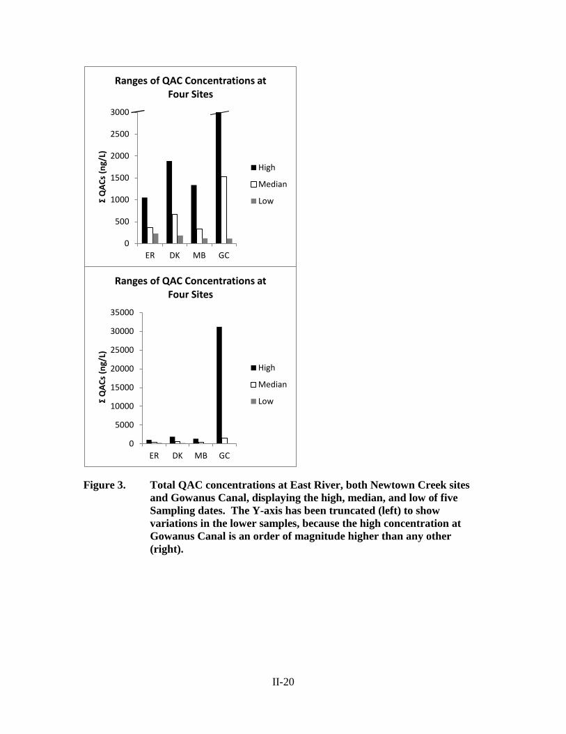
Figure 3. Total QAC concentrations at East River, both Newtown Creek sites and Gowanus Canal, displaying the high, median, and low of five Sampling dates. The Y-axis has been truncated (left) to show variations in the lower samples, because the high concentration at Gowanus Canal is an order of magnitude higher than any other

(right).

0

500

1000

1500

2000

2500

3000

ER DK MB GC

Ʃ Q

ACs

(ng/

L)

Ranges of QAC Concentrations at Four Sites

High

Median

Low

0

5000

10000

15000

20000

25000

30000

35000

ER DK MB GC

Ʃ Q

ACs

(ng/

L)

Ranges of QAC Concentrations at Four Sites

High

Median

Low

II-20

Figure 4. Labile fraction of QACs as a function of recent rainfall at East River, both Newtown Creek sites and Gowanus Canal, displaying the high, median, and low of five sampling dates.

Figure 5. Relationship between labile fraction of QACs and prior-day rainfall in the East River, both Newtown Creek Stations, and Gowanus Canal. Comparisons of mean values were determined for four of the dates where n=4 using a standard t-test conducted in Excel; the mean of the labile fraction percentage from the high-rain data set from May differs significantly from the low rain sets in June (P=0.0067) and October (P=0.0038); a higher mean for the labile fraction in May than that observed in August (0.6 inches of rain) was close to being

significant (P = 0.058).

0%

10%

20%

30%

40%

50%

60%

ER DK MB GC

Labi

le F

ract

ion

Ranges of QAC Compositions at Four Sites

High

Median

Low

y = 0.2738x + 0.0654 R² = 0.6986

0%

10%

20%

30%

40%

50%

60%

0 0.2 0.4 0.6 0.8 1 1.2

Labi

le F

ract

ion

Prior day Rainfall (inches)

Relationship Between Prior Day Rainfall and QAC Composition

II-21

Figure 6. Natural logarithm relationship between concentrations of behentrimonium and Enterococcus. Includes East River, both Newtown Creek sites, and Gowanus Canal.

Figure 7. Logarithmic relationship between the abundance of Enterococcus and prior day rainfall, at the East River, both Newtown sites, and

Gowanus Canal.

Dissolved phase QACs were successfully detected in some samples, including the

August Piermont (Figures 8, 9), August Gowanus Canal, and the sample taken at the

y = 0.4468x + 2.4993 R² = 0.5054

2

3

4

5

6

7

8

9

10

0 2 4 6 8 10 12

Ln [b

ehen

trim

oniu

m] (

ng/L

)

Ln [Enterococcus] (cells/ 100 ml)

Relationship Between Behentrimonium and FIB Concentrations

y = 3.2762x + 3.8142 R² = 0.2917

0.00

2.00

4.00

6.00

8.00

10.00

12.00

0 0.2 0.4 0.6 0.8 1 1.2

Ln(E

nter

ococ

cus)

cel

ls/1

00m

l

Prior day rainfall (inches)

Relationship Between FIB Concentrations and Prior Day Rainfall

II-22

125th St. CSO outfall during the North River accident. Preliminary data indicates that the

dissolved phase detections were poor in all samples taken during October. At Piermont,

the smallest QAC, ATMAC 12, is entirely found in the dissolved phase, while the larger

DADMACs are associated primarily with the particulate phase (<12% dissolved). Such

results could explain why the labile fractions determined in CSO affected waters were

lower than expected.

Figure 8. Concentrations of nineteen different QACs in a sample taken at Piermont. Measurements in the particulate and dissolved phases for each analyte are shown adjacent to each other.

Figure 9. Partitioning of nineteen different QACs between the dissolved and particulate phases in a water sample taken at Piermont.

0100020003000400050006000

Conc

entr

atio

n (n

g/L)

August QAC Concentrations at Piermont

Particulate

Dissolved

0%20%40%60%80%

100%

% o

f tot

al

Particulate vs. Dissolved Partitioning at Piermont (8/16/2011)

% Dissolved

% Particulate

II-23

Results from sampling conducted at approximately 125th St. during the North

River accident are illustrated in Figure 10. The concentrations are seen to have fallen

sharply with distance from the CSO, and the change of composition is consistent with a

loss of more labile components upon dilution. It should be noted that the concentrations

of total QACs in the main stem of the river was not dramatically elevated over average

levels measured in the lower estuary and the water in the river had experienced a couple

days of input of untreated sewage.

Figure 10. Changes in QAC composition and concentration with distance from a point source discharge near the North River WWTP during its July 2011 failure. These samples were taken near the end of the three-day

discharge.

0

1

2

3

4

5

0%

10%

20%

30%

40%

50%

60%

0 50 100 150

LOG

[Tot

al Q

ACs]

(ng/

L)

Labi

le F

ract

ion

Distance from point source (m)

Changing Conditions with Distance from Raw Sewage Discharge

Labile fraction

Total QACs

II-24

DISCUSSION

A significant result of this project is that the first successful detections of QACs

were made in estuarine surface waters in the U.S. or anywhere in the world.

Furthermore, the relationship between QAC composition and prior day rainfall at the

Brooklyn sites suggests that CSO discharge causes surface waters to become measurably

enriched in the more labile QACs which would otherwise be more depleted in waters

impacted by treated sewage (Figure 5). This enrichment of the labile fraction appears

muted at the East River site (Figure 4), because it receives a mixture of treated and

untreated sewage during large CSO events. A second piece of evidence to support this

idea is the fact that the East River experiences less variation in the total concentration of

QACs, compared to the Newtown and Gowanus sites (Figure 3). The constant input of

treated sewage into the East River has a dominant effect on the QAC

concentration/composition of that water body, even when untreated sewage is added.

Dissolved phase measurements, although limited in number of samples, provided

some useful information. At Piermont, a high level of dissolved QACs was discovered in

August (Figure 8). The dissolved-particulate partitioning, the high labile fraction seen

especially in the dissolved phase, and the large total concentration of QACs suggest that

poorly-treated sewage was being discharged into the river at this time. The prior day saw

0.6 inches of rain, and two days prior there was a record-setting rainfall of 6.4 inches, so

it is possible that a CSO discharge was responsible for this untreated sewage signal, or

that the local WWTP became overloaded and there was some bypass of untreated

sewage. In contrast, samples taken there in June had a much lower total concentration

and a lower labile fraction, resembling a treated sewage source (although no dissolved-

II-25

phase measurements were made that day). This further suggests that rainfall can have an

adverse effect on water quality at Piermont, but more information about the sewage

treatment operations and a larger number of samples are needed to test this. Dissolved

phase measurements made during a drier period in October did not detect any of the

analytes except the most abundant ones; however, the data for dissolved phase

measurement are very preliminary, and it is unclear if analytical sensitivity was sufficient

for this sample set. Further work must be done to perfect the dissolved phase analysis.

At the North River site, a dramatic change in the QAC population of the water

column was observed during the July raw sewage discharge. At the discharge point

source, the composition was enriched in the more labile QACs, relative to samples taken

at the point source there in June or August. However, this enrichment dissipated rapidly

with distance from the outfall, having attenuated to background levels (below the harbor-

wide median of 19%) within 111m (Figure 10). Dilution is a likely cause of this

attenuation. At the time of sample collection, discharge had already been happening for

two days. Freshly discharged particles were mixed with sewage-derived QACs which

had entered the estuary on previous days, and those older QACs were likely depleted in

labile compounds due to time spent in the river. At the Dyckman St. Beach, there was a

similar compositional change during the July failure event (30% labile QACs vs. 19%

during August), but the total concentration of QACs was unchanged; it is possible that

the discharge was beginning to diminish at the time of sampling as the WWTP came back

into operation.

II-26

Figure 11. Average QAC composition across several kinds of water samples, with particulate-phase measurements. (1) Influent taken from a WWTP on Long Island; (2) Effluent taken from that same WWTP after undergoing tertiary treatment; (3) Samples taken from the North River sites on July 22nd during the raw sewage discharge; (4) Highly contaminated sample found at the Piermont outfall during August; (5) Samples taken at Newtown Creek and Gowanus Canal after a pronounced CSO event in May, (6) Samples taken from the canals in August, after a lesser rainfall than May; (7) Samples taken from the canals during drier periods; (8) Samples taken during any weather in the East River and Hudson River (9) Sediment samples from CSO-impacted sites around NY/NJ harbor; (10) Sediment samples taken from non-CSO sites around NY/NJ harbor.

Comparisons across sites (Figure 11) are a useful way of considering the data.

Included for illustrative purposes, the WWTP influent and effluent cannot be directly

compared to sites from New York City, since the plant in question receives low flows and

different sewer shed inputs, and uses a different kind of treatment, but nonetheless it

indicates that compositional differences between treated and untreated sewage are

substantial. The highly contaminated samples from Piermont and the North River

accident have a labile fraction that is quite high, especially considering the amount of

0% 10% 20% 30% 40% 50% 60% 70% 80% 90%

NY/NJ Non-CSO Sed (10)NY/NJ CSO Sed (9)Non-CSO Sites (8)Canals No rain (7)Canals August (6)

Canals May (5)Piermont August (4)

North River Accident (3)WWTP Effluent (2)WWTP Influent (1)

Labile fraction

Comparison of Compositions Across 10 kinds of samples

II-27

dilution that occurs in some of those samples upon discharge. In the canals, May

compositions were labile QAC-enriched compared to dry weather compositions, which

yielded compositions very similar to those found at non-CSO sites. Unexpectedly, the

August canal samples also resembled dry-weather compositions. Either the 0.6-inch

rainfall the day before was not sufficient to trigger a large CSO event, degradation of the

labile QACs occurred rapidly between the rain and the time of sampling, or after

approximately a tidal cycle, the CSO signal in the canals was sufficiently diluted with

surrounding water that the signal was masked. Since the microbial populations of the

canals are highly acclimated to sewage contaminants, it is possible that labile QACs have

a shorter residence time in the canals than in less-impaired waterways. Sediment

measurements from non-CSO sites resemble the compositions found in the water column

during dry periods or away from CSO sites. Finally, prior sediment measurements made

near CSO outfalls had an intermediate composition, being more labile-enriched than dry-

weather water, but less enriched than CSO water. This intermediate composition may

reflect further loss of labile QACs prior to or after deposition, or that what is deposited

near the CSOs represents mixed input of QACs to the sediment in such sites, as the water

column above sees a range of concentrations and compositions depending on rainfall.

Compositional changes were generally not as pronounced as expected, based on

comparisons between raw sewage and treated sewage samples taken inside of WWTPs.

One possible explanation is that the difference would be greater if dissolved phase

measurements had been included. Since the most degradable QACs are also the most

soluble, they may have a more telling presence than anticipated in the dissolved phase,

particularly for fresh sewage discharge.

II-28

ACKNOWLEDGMENTS

This research would not have been possible without the help of Riverkeeper’s

John Lipscomb, who took me sampling. I also need to thank Dr. Gregory O’Mullan, Dr.

Andrew Juhl, and their FIB monitoring team, for providing data, and my fellow students

Anne Cooper Doherty and Shawn Fisher, for their support and advice.

II-29

REFERENCES

Clara, M., S. Scharf, C. Scheffknecht, and O. Gans. 2007. Occurrence of selected surfactants in untreated and treated sewage. Water Research 41:4339-4348.

Donovan, E., D.F. Stakal, K.M. Unice, J.D. Roberts, C. Haws, B. Finley, and M. Harris. 2008. Risk of gastrointestinal disease associated with exposure to pathogens in the sediment of the lower Passaic River. Applied and Environmental Microbiology. 74:1004-1018.

Ferrer, I. and E.T. Furlong. 2001. Identification of alkyl dimethylbenzylammonium surfactants in water samples by solid-phase extraction followed by ion trap LC/MS and LC/MS/MS. Environmental Science and Technology 35:2583-2588.

Freis J.S., G.W. Characklis, and R.T Noble. 2008. Sediment-water exchange of Vibrio sp. and fecal indicator bacteria: Implications for persistence and transport in the Neuse River Estuary, North Carolina, USA. Water Research 42:941-950.

Haack, S.K., J.W. Duris, L.R. Foarty, D.W. Kolpin, M.J. Focazio, E.T. Furlong, and M.T. Meyer. 2009. Comparing wastewater chemicals, indicator bacteria concentrations, and bacterial pathogen genes as fecal pollution indicators. Journal of Environmental Quality 38:248-258.

Hagerdorn, C., and S.B. Weisberg. 2009. Chemical-based fecal source tracking methods: current status and guidelines for evaluation. Reviews in Environmental Science & Biotechnology 8:275-287.

Jarrol, E.L., A.K. Bingham, and E.A. Meyer. 1981. Effect of chlorine on Giardia lamblia cyst viability. Applied and Environmental Microbiology 41:483-487.

Jeng, H.C., A.J. England, and H.B. Bradford. 2005. Indicator organisms associated with stormwater suspended particles and estuarine sediments. Journal of Environmental Science and Health, Part A 40:779-791.

Li, X. 2009. Quaternary ammonium compounds (QACs) in marine sediments: detection, occurrence and application as geochemical tracers. Doctoral dissertation. Stony Brook University, Stony Brook, New York.

Li, X., and B. Brownawell. 2009. Analysis of quaternary ammonium compounds in estuarine sediments by LC-ToF-MS: Very high positive mass defects of alkylamine ions as powerful diagnostic tools for identification and structural elucidation. Analytical Chemistry 81:7926–7935.

II-30

Li, X., and B. Brownawell. 2010. Quaternary ammonium compounds in urban estuarine sediment environments - a class of contaminants in need of increased attention? Environmental Science and Technology 44:7561-7568.

Lara-Martin, P., X. Li, R. Bopp, and B. Brownawell. 2010. Occurrence of alkyltrimethylammonium compounds in urban estuarine sediments: behentrimonium as a new emerging contaminant. Environmental Science and Technology 44:7569-7575.

McLellan, S., E. Hollis, M. Depas, M. Van Dyke, J. Harris, and C. Scopel. 2007. Distribution and fate of Escherichia coli in Lake Michigan following contamination with urban stormwater and combined sewer overflows. Journal of Great Lakes Research 33:566–580.

NYCDEP. 2010. New York Harbor Water Quality Report. New York City Department of Environmental Protection.

Simpson, J.M., J.W. Santo Domingo, and D.J. Reasoner. 2010. Microbial source tracking: state of the science. Environmental Science and Technology 36:5279- 5288.

Stoeckel, D.M., and V.J. Harwood. 2007. Performance, design, and analysis in microbial source tracking studies. Applied and Environmental Microbiology 73:2405-2415.

Swartz C.H., S. Reddy, M.J. Benotti, H. Yin, L.B. Barber, B. Brownawell, and R. Rudel. 2006. An analysis of steroid estrogens, alkylphenols, and other wastewater contaminants leaching into groundwater from a residential septic system on Cape Cod, MA. Environmental Science and Technology 40:4894-4902.

Wheeler, A.L., P.G. Hartel, D.G. Godfrey, J.L. Hill, and W.I. Segars. 2002. Potential of Enterococcus faecalis as a human fecal indicator for microbial source tracking. Journal of Environmental Quality 31:1286–1293.

II-31

ASSESSMENT OF TEMPORAL AND GEOGRAPHIC POPULATION STRUCTURING OF PHRAGMITES AUSTRALIS ALONG THE

HUDSON RIVER USING MICROSATELLITE DNA MARKERS

A Final Report of the Tibor T. Polgar Fellowship

Daniel Lipus

Polgar Fellow

Department of Biology Iona College

New Rochelle, NY

Project Advisors: Joseph Stabile

Department of Biology Iona College

New Rochelle, NY

Isaac Wirgin Department of Environmental Medicine

New York University School of Medicine Tuxedo, NY, 10987

Lipus, D., J. Stabile and I. Wirgin. 2012. Assessment of temporal and geographic population structuring of Phragmites australis along the Hudson River using microsatellite DNA markers. Section III: 1-27 pp. In D.J. Yozzo, S.H. Fernald, and H. Andreyko (eds.), Final Reports of the Tibor T. Polgar Fellowship Program, 2011. Hudson River Foundation.

III-1

ABSTRACT

Phragmites australis is a perennial grass that has been spreading significantly

throughout wetlands of the Northeastern United States within the last 100 years. For the

Hudson River populations, previous studies have suggested high genetic variability

within and among populations, as a reason for its dramatic spread. In this study, samples

were collected from nine locations along the Hudson River and its surrounding areas.

These, as well as samples collected in 2004 from the same locations, were analyzed for

genetic variability using microsatellite primers for eight different loci. Results showed

that populations growing in the northern regions of the Hudson River are genetically

different from populations growing in the southern Hudson River regions. Comparison of

2004 and 2011 samples suggested that several populations have evolved over the last

seven years. All samples were found to be of the invasive genotype suggesting that native

populations are rare or not present in and around the Hudson River Valley. Based on high

genetic variability, seed dispersal was proposed to be an important spread mechanism for

Hudson River populations supporting previous studies.

III-2

TABLE OF CONTENTS

Abstract ........................................................................................................................ III-2

Table of Contents ......................................................................................................... III-3

List of Tables and Figures ............................................................................................ III-4

Introduction .................................................................................................................. III-5

Methods........................................................................................................................ III-9

Results .......................................................................................................................... III-11

Discussion .................................................................................................................... III-20

Acknowledgements ...................................................................................................... III-25

References .................................................................................................................... III-25

III-3

LIST OF FIGURES

Figure 1. Ethidium bromide stained minigel of 11 PCR products using microsatellite primers PAGT-12, PAGT-13 and PAGT-22 ................... III-12

Figure 2a. DNA sequencer output showing homozygous alleles for loci 12, 13 and 22. Each colored peak represents the size of a DNA fragment for a particular locus ............................................................................. III-13

Figure 2b. DNA sequencer output showing heterozygous alleles for loci 12, 13 and 22. Each colored peak represents the size of a DNA fragment for a particular locus ............................................................................. III-14

Figure 2c. DNA sequencer output showing multiple alleles for locus 12 ............. III-15

Figure 5. UPGMA tree based on microsatellite data for the analyzed Hudson River Populations and its surrounding regions .................................... III-19

LIST OF TABLES

Table 1. Sampling sites from 2004 and 2011 collections .................................. III-9

Table 2. Microsatellite primer sets and PCR conditions used by McCormick et al. (2010) from Saltonstall (2003) ................................ III-10

Table 3. Raw data showing allele sizes of 8 different loci for 7 different populations.......................................................................... III-16

Table 4. Comparison for number of alleles observed in this study by McCormick et al. (2010). Differences are marked in red ............... III-16

Table 5.1-5.3 Results of population differentiation analysis for 2004 samples (5.1) , 2011 samples (5.2) and combined data (5.3). Listed populations showed significant differences to each other based on highly significant differences and P-values (P< 0.0001)………………………………………….III-17-18

III-4

INTRODUCTION

Phragmites australis is a tall perennial grass of the Poacaea family and is also

known as “giant reed” or “common reed.” Phragmites is one of the most productive

species of plants on earth (Hartog 1989). Today, it is distributed all over the mainland

US as well as through southern Canada (Wilcox et al. 2003). In many areas, it has

become the dominant plant of freshwater and brackish marshes at the exclusion of other

genera such as Typha and Spartina (Stanne et al. 1996). Even though fossil records show

that the plant has been in the U.S. for about 40,000 years, its abundance has increased

dramatically since the early 1900’s (Saltonstall 2002).

This plant has had great ecological success because it can colonize even small

patches of disturbed soils very quickly (Kettenring et al. 2010). Phragmites alters the

habitat to promote its own growth by modifying the sulfide, carbon, oxygen and moisture

characteristics of soils as its populations become established (Osgood et al. 2003). Once

established, Phragmites populations can maintain dense stands (200-300 culms/m2)

through the propagation of its rhizomes. This biomass can cause the shoots to exceed

living plants resulting in a thick mat that not even new Phragmites can penetrate (Haslam

1972). Not only does Phragmites affect the type of plants that grow in its habitat, it also

affects the animal life as well. A study done by Wells et al. (2008) suggests that

Phragmites has greatly reduced the number avian species diversity in some tidal marshes

along the Hudson River including Iona Island and Constitution Marshes. Some

researchers agree that this plant is an invasive nuisance and reduces the biodiversity of

III-5

wetlands and thus many regions around the country have implemented programs to

monitor and reduce its expansion (Marks et al. 1994; Chambers 1999; Meyerson et al.

2000). However, some scientists dispute the necessity of aggressive removal of

Phragmites. Kiviat has illustrated that many species use Phragmites as a food source and

habitat and that complete removal can have severe consequences to a community (Kiviat

and MacDonald 2003; Kiviat 2010).

The Hudson River and the surrounding New York/New Jersey region provide a

diverse array of habitats that Phragmites has been able to colonize. Soil habitats can

range from polluted to non-polluted and salinity can range from brackish to freshwater.

The distribution and abundance of Phragmites along the Hudson River has grown

dramatically since the 1970s because it has been able to colonize a variety of habitats

presented to it. It has been so successful that it is now predicted to become the dominant

wetlands plant in the tidal Hudson River in the next few decades (Kiviat 2010). The

mechanisms that have allowed it to spread so rapidly will not fully be understood without

characterizing the genetics of its populations.

Saltonstall (2002; 2003a; 2003b) was the first researcher to genetically

characterize P. australis using chloroplast and microsatellite DNA markers. She first

characterized chloroplast DNA (cpDNA) from Phragmites samples collected all over the

globe (Saltonstall 2002). From this study, Saltonstall characterized 27 cpDNA

haplotypes, one of which, Haplotype M, was identified as the Eurasian variety that is now

invasive in the Northeast United States. A Restriction Fragment Length Polymorphism

(RFLP) technique was also developed to easily distinguish between native and invasive

varieties (Saltonstall 2003b). This RFLP technique confirmed that the vast majority of

III-6

Phragmites in the Northeast are descended from the Eurasian lineage. However, a recent

study has identified native P. australis populations in freshwater and oligohaline marshes

of Delaware and southern New Jersey (Meadows and Saltonstall 2007).

Saltonstall also developed a set of microsatellite primers to characterize the

nuclear genome of P. australis. This method confirmed diversity among P. australis

individuals and that native and invasive varieties did not form hybrids (Saltonstall 2003a).

However, the focus of this study was to compare native, invasive and gulf populations of

Phragmites and did not closely examine populations within a particular river system.

P. australis populations from the Rhode River, a brackish sub-estuary of the

Chesapeake Bay, have been characterized using microsatellite DNA (McCormick et al.

2010). McCormick used eight primers (designed by Saltonstall 2003a) to amplify

microsatellite regions in P. australis. Her analysis illustrated that P. australis

populations followed an isolation-by-distance model. Populations in close proximity

were more closely related than those at greater distances. The genetic analyses and

mapping of P. australis populations supported the importance of seed dispersal rather

than vegetative propagation. Patches growing in isolation were found to be genetically

unique confirming the establishment by seed. Using satellite images, McCormick was

able to analyze P. australis expansion over the last 35 years. It was found that P.

australis populations have expanded rapidly since 1971. High genetic variation and the

rapid spread of P. australis populations lead to the conclusion that the invasive varieties

have responded to environmental changes (McCormick et al. 2010).

To date, only one study has examined the genetic structure of Hudson River

Phragmites populations (Maltz and Stabile 2005). Three ISSR primers were used to

III-7

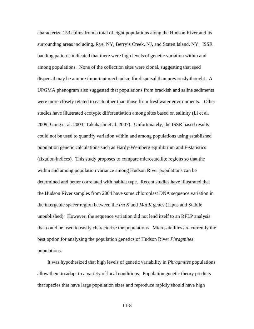
characterize 153 culms from a total of eight populations along the Hudson River and its

surrounding areas including, Rye, NY, Berry’s Creek, NJ, and Staten Island, NY. ISSR

banding patterns indicated that there were high levels of genetic variation within and

among populations. None of the collection sites were clonal, suggesting that seed

dispersal may be a more important mechanism for dispersal than previously thought. A

UPGMA phenogram also suggested that populations from brackish and saline sediments

were more closely related to each other than those from freshwater environments. Other

studies have illustrated ecotypic differentiation among sites based on salinity (Li et al.

2009; Gong et al. 2003; Takahashi et al. 2007). Unfortunately, the ISSR based results

could not be used to quantify variation within and among populations using established

population genetic calculations such as Hardy-Weinberg equilibrium and F-statistics

(fixation indices). This study proposes to compare microsatellite regions so that the

within and among population variance among Hudson River populations can be

determined and better correlated with habitat type. Recent studies have illustrated that

the Hudson River samples from 2004 have some chloroplast DNA sequence variation in

the intergenic spacer region between the trn K and Mat K genes (Lipus and Stabile

unpublished). However, the sequence variation did not lend itself to an RFLP analysis

that could be used to easily characterize the populations. Microsatellites are currently the

best option for analyzing the population genetics of Hudson River Phragmites

populations.

It was hypothesized that high levels of genetic variability in Phragmites populations

allow them to adapt to a variety of local conditions. Population genetic theory predicts

that species that have large population sizes and reproduce rapidly should have high

III-8

levels of genetic variation. Genetic variation should allow Phragmites populations to

adapt to the variety of environmental conditions found along the Hudson River. This

hypothesis was tested using the microsatellite primer developed by Saltonstall (2003a)

and recently used by McCormick et al. (2010) to characterize the 2004 sample set and

compared it to new samples taken from the same Hudson River sites in 2011.

METHODS Sample Collection

A minimum of 40 culms were collected at each site following transects through

the center of the population and along the perimeter. Approximately 20 culms were am-

plified from each site and this appeared to be adequate to identify the different microsat-

ellite alleles. The area occupied by each population was demarcated using a GPS for fu-

ture reference.

Table 1. Sampling sites from 2004 and 2011 Collections

Sites Habitat Tivoli Bays Fresh Water

Constitution Island/Cold Spring Marsh

Fresh Water

Iona Island Marsh Fresh Water Piermont Marsh Fresh Water Berry’s Creek Brackish Passaic River Brackish

Rye Marsh Salt Water Richmond Salt Water

Albany Fresh Water

III-9

Microsatellite Analysis Table 2. Microsatellite primer sets and PCR conditions used by McCormick et al

(2010) from Saltonstall. (2003a).

Primer Annealing Temperature (oC)

Alleles

PaGT4 50 5 PaGT9 50 7 PaGT12 56 5 PaGT13 50 6 PaGT14 58 5 PaGT16 56 8 PaGT21 58 11 PaGT22 50 8

For microsatellite analysis, PCR reactions were carried out with a volume of 12.5

ul, with 50 ng or less of template DNA, 1 X PCR buffer (10 mM Tris-HCl, pH 8.3, 50

mM KCl) 2 mM MgCl2, 0.25 mM dNTPs, 05 mM forward and reverse primers and 0.1 U

Taq DNA polymerase. PCRs were performed as single reactions and then subsequently

pooled prior for microsatellite analysis. Characterization of microsatellite genotypes was

done on a Beckman Coulter CEQTM8000 capillary-based DNA sequencer. Multiplexed

PCR reactions were diluted up to 1:3 with Sample Loading Solution (Beckman Coulter),

0.5 to 2 ul of diluted PCR reactions were loaded onto 96 well plates along with 0.5 ul of

CEQ DNA Size Standard-400 (Beckman Coulter) and 40 ul of Sample Loading Solution

(Beckman Coulter) and run with the FRAG 1 program. Microsatellite data was analyzed

for population differentiation using GenePop (Raymond and Rousset 1995). An UPGMA

tree was generated using Poptree (Takezaki et al. 2010).

III-10

RESULTS

About 90% of amplified samples yielded usable PCR products. The quality of PCR

products was initially analyzed using agarose gel electrophoresis. Figure 1 illustrates the

PCR products representative of those used in microsatellite analyses. 332 of the collected

372 culms (184 from 2004 and 188 from 2011) were analyzed. Sets of two or three loci

were analyzed at the same time simultaneously in the DNA sequencer. Data output

showed alleles of each locus in a different color. Each peak stood for one fragment size

and one locus. Overall loci were observed to be either homozygous, heterozygous or had

more than two alleles at each locus probably due to alloploidy. Figures 2a, b and c show

typical DNA sequencer outputs for those three cases. Blue peaks represent size alleles for

locus 12 alleles, green peaks represent the different size alleles locus 13 alleles and the

black peaks represent the size for locus 22.

III-11

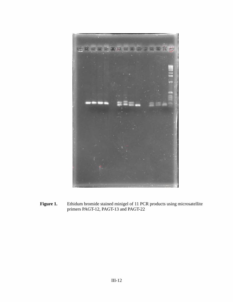
Figure 1. Ethidum bromide stained minigel of 11 PCR products using microsatellite primers PAGT-12, PAGT-13 and PAGT-22

III-12

Figure 2a. DNA sequencer output showing homozygous alleles for loci 12, 13 and 22. Each colored peak represents the size of a DNA fragment for a particular locus.

III-13

Figure 2b. DNA sequencer output showing heterozygous alleles for loci 12, 13 and 22. Each colored peak represents the size of a DNA fragment for a particular locus.

III-14

Raw data for each sample and locus were recorded for further data analysis.

Table 3 shows the alleles for samples 471 to 490 (Berry’s Creek populations) for all eight

loci. The data showed that some loci had mulitple alleles (>2) and some loci had

individual alleles for those samples. Microsatellite analysis of samples for loci PAGT-4

and PAGT-9 has not been concluded yet, and results for these loci were not included in

Figure 2c. DNA sequencer output showing multiple alleles for locus 12.

III-15

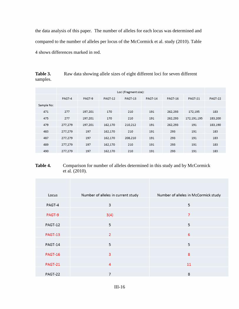
the data analysis of this paper. The number of alleles for each locus was determined and

compared to the number of alleles per locus of the McCormick et al. study (2010). Table

4 shows differences marked in red.

Table 3. Raw data showing allele sizes of eight different loci for seven different samples.

Differences are marked in red. Table 4. Comparison for number of alleles determined in this study and by McCormick et al. (2010).

III-16

Table 5.1-5.3. Results of population differentiation analysis for 2011 sample (5.1) , 2004 samples (5.2) and combined data (5.3). Listed populations showed significant differences from each other. Populations were considered significantly different with a P value < 0.0001.

2011 Populations 2011 PopulationsRye Marshlands Rye Marshlands

Piermont Iona IslandAlbany Iona Island

Iona Island PiermontCold Spring Piermont

Albany AlbanyTivoli Bays Albany

Albany AlbanyRye Marshlands Tivoli Bays

Passaic River Tivoli BaysBerry’s Creek Tivoli Bays

Tivoli Bays Tivoli BaysPiermont Tivoli Bays

Cold Spring Tivoli BaysAlbany Tivoli Bays

Tivoli Bays Cold SpringIona Island Cold SpringPiermont Cold Spring

Tivoli Bays Cold Spring

VS

2004 Populations 2004 PopulationsBerry’s Creek RichmondPassaic River Cold SpringBerry’s Creek Cold Spring

Tivoli Bays Cold SpringRichmond Cold Spring

Rye Marshlands AlbanyPassaic River AlbanyBerry’s Creek Albany

Tivoli Bays AlbanyRichmond AlbanyPiermont Albany

VS

III-17

2004 Populations 2011 PopulationsRye Marshlands Berry’s Creek

Piermont Berry’s CreekIona Island Berry’s Creek

Albany Berry’s CreekCold Spring Passaic River

Albany Passaic RiverTivoli Bays Rye

Albany RyeRye Marshlands Iona IslandPassaic River Iona IslandBerry’s Creek Iona Island

Tivoli Bays Iona IslandRichmond Iona IslandPiermont Iona Island

Cold Spring PiermontAlbany Piermont

Tivoli bays RichmondBerry’s Creek Albany

Piermont AlbanyCold Spring Albany

Albany AlbanyRye Marshlands Tivoli BaysPassaic River Tivoli BaysBerry’s Creek Tivoli Bays

Tivoli Bays Tivoli BaysRichmond Tivoli BaysIona Island Tivoli BaysCold Spring Tivoli Bays

Albany Tivoli BaysRye Marshlands Cold SpringBerry’s Creek Cold Spring

Tivoli Bays Cold SpringCold Spring Cold Spring

Albany Cold Spring

VS

III-18

Allele data for six loci (12, 13, 14, 16, 21 and 22) were analyzed using Genepop

for population differentiation. Results showed highly significant differences in the

frequencies of alleles among multiple pair-wise populations’ comparisons. Comparison

of 2004 samples indicated that the Albany and Cold Spring populations were most

different from all the other populations. Highly significant temporal differences between

populations were also observed in comparisons between populations from the 2004 and

2011 samples. Specifically, the allele frequencies of the Albany, Cold Spring and Tivoli

Bays populations changed over the last seven years.

Figure 5. UPGMA tree for the analyzed Hudson River Populations. Bootstrapping values of 50 or greater are shown at the nodes.

III-19

Analysis of the 2011 samples suggested that Albany, Cold Spring and Tivoli Bays

were most different from the remaining populations. Figure 3 lists the populations’

comparisons showing highly significant differences (P-value < 0.05).

An UPGMA tree was constructed based on the population differentiation test

results. Results showed that every patch, regardless of size, had multiple phenotypes.

2004 and 2011 P. australis populations from Rye, Passaic River, Piermont, Richmond

and Berry’s Creek were found to be genetically similar (Figure 5). 2011 Cold Spring,

Albany and Tivoli bays populations were found to be genetically different from the 2004

populations based on the UPGAM analysis. Cold Spring was determined to be

genetically isolated from the other populations.

Neither native microsatellite allele phenotypes nor endemic genotypes were

present in the analyzed sample. All samples were shown to be of the invasive genotype.

DISCUSSION

Analysis of six microsatellite loci for samples from nine different locations collected at

two different times supports the hypothesis that P. australis populations have high levels of

genetic variability. Due to the fact that the analyzed populations grow in different habitats this

project supports the theory that genetic variability allows populations to adapt and spread along a

variety of local conditions along the Hudson River. Analysis of allele differences suggested that

there is significant diversity within sites and patches. Variability among patches was determined

to be greater than within patches.

High numbers of alleles in both homozygous and heterozygous conditions were also

III-20

observed. The number of different alleles determined in this study was smaller than those

observed by McCormick et al. (2010). It is difficult to determine the reason that fewer genotypes

were observed in the Hudson River populations as compared to the Rhode River. Some possible

factors could be differences in habitat and climate between the two river systems. Additionally,

Hudson River populations may have lost some genotypes due to stochastic mechanisms such

genetic drift or founder effects. Allele sizes for most loci were found to be in the vicinity of the

data reported by Saltonstall (2002). No samples were found to exhibit allele sizes common to

native genotypes confirming that no or very few native P. australis populations exist in the

Northeast (Saltonstall 2002) or along the Hudson River (Kiviat 2010).

Population differentiation analysis suggested a geographic pattern for population

structuring. Microsatellite analysis of the 2004 sample set indicated significant differences

between the populations located along the northern Hudson River (Albany, Cold Spring) and the

remaining populations located closer towards New York City. Also, Albany and Cold Spring

populations did not exhibit any significant differences to each other. Interestingly, Tivoli Bays

populations, which are geographically located between the Albany and Cold Springs populations,

were found to be significantly different from either but did not show any significant differences

to the other analyzed populations. Richmond populations were found to be significantly

different from Albany, Cold Spring and Berry's Creek populations. Based on these data, it was

suggested that populations from fresh water regions (northern Hudson River Estuary) are

genetically different from populations growing in brackish water regions. Richmond populations

are exposed to the highest salinity levels due to their location near the New York Bight.

Furthermore, Richmond populations are exposed to different and higher levels of pollutants than

most of the other populations, which could be one of the reasons why they were found to be

III-21

genetically different. The presented data suggests a connection between the diverse

environments and the genetic variability. Results regarding population clustering confirm the

data reported by Maltz and Stabile (2005), yet the Cold Spring populations were shown to be

significantly different from Iona Island and Tivoli Bays population, which was not reported in

the 2005 study.

For the 2011 samples, a similar geographic pattern was observed. Freshwater populations

located further north in the Hudson River Estuary(Tivoli Bays, Cold Spring and Albany) were

significantly different from the other populations located closer to New York City. In addition,

the Iona Island populations were significantly different both from populations located further

north (Albany, Tivoli Bays and Cold Spring) and from populations located along the southern

Hudson River Estuary (Piermont). Among the 2004 samples, Cold Spring and Albany

populations were not significantly different from each other but were found to be significantly

different from the Tivoli Bays populations, suggesting they must be genetically isolated. The

general pattern of northern freshwater populations showing genetic differences in comparison to

southern brackish water populations was confirmed; however, several populations seem to have

evolved and show significant differences to the majority of the other populations contradicting

the clustering proposed by Maltz and Stabile (2005).

The Iona Island, Piermont and Tivoli Bays populations seem to be evolving. They did

not show any significant differences to their surrounding populations in 2004 but were found to

be different in 2011. The 2011 samples also suggested significant differences between the Rye

Marsh populations and most other analyzed populations, which is not surprising due to the

population’s location along the Long Island Sound and its geographical isolation from the

Hudson River.

III-22

UPGMA tree analysis suggests that 2011 Cold Spring populations are genetically isolated

from the other populations. This result is surprising because the population is not geographically

isolated. It is located between Tivoli Bays and Albany. Reasons for the genetic differences could

be the history of the Constitution marsh including its contamination in the 50’s and 60’s and the

resulting remediation projects.

Direct allele comparison of the 2004 and 2011 samples showed many differences between

populations. Most importantly it was determined that 2011 Albany, Tivoli Bay and Cold Spring

populations were significantly different from 2004 populations from the same locations.

UPGMA tree analysis supported this hypothesis. 2004 and 2011 populations from Albany, Tivoli

Bays and Cold Spring were found to be genetically different. 2004 and 2011 from Rye, Passaic

River, Staten Island and Berry’s Creek Populations were clustered together in the tree and

therefore considered genetically similar. This suggests that the northern Hudson River Estuary

populations have changed within the last seven years. Reasons for the rapid change could be

environmental or external factors such as pollution and habitat restoration. Genetic drift also has

to be considered as one of the reasons for increased differences between populations. The

remaining populations did not show any change within the last seven years suggesting that these

populations have reached genetic equilibrium.

Previous studies have suggested that seed dispersal has to be considered an important

mechanism by which Phragmites can spread. Researchers came to this conclusion due to high

genetic variability within stands of P. australis and among populations (Maltz and Stabile 2005;

McCormick et al. 2010). No single stand was observed to be monoclonal and individuals with

different genotypes were collected in very close proximities within stands. Results of this study

support this hypothesis based on the fact that P. australis populations growing along the Hudson

III-23

River were found to exhibit considerable genetic variability. Studies monitoring P. australis

populations along the Rhode River reported that establishment by seed dispersal has been more

common in populations influenced by human activities (McCormick et al. 2010). Furthermore, it

was determined that seed viability was greater among Phragmites populations with greater

genetic variation. This study did not examine the correlation between genetic variation and seed

viability. Populations growing along the upper Hudson River Estuary showed more differences

to each other than populations growing along the lower Hudson River Estuary, suggesting that

seed dispersal could be the primary mechanism of spread within this area. To obtain more exact

data regarding those parameters a more detailed analysis is necessary.

The project showed that P. australis populations along the Hudson River are diverse and

have the ability to evolve. A general pattern shows population clustering with the populations

growing along the upper Hudson River Estuary (Albany, Cold Spring, Tivoli Bays) being

significantly different to populations growing along the lower Hudson River Estuary. Analysis

of the 2011 samples showed that more populations started to evolve independently within the last

seven years and show fewer similarities to populations in close proximity. No native phenotypes

or genotypes were discovered supporting studies by Saltonstall (2002) and Kiviat (2010) which

state that the invasive haplotype M is the most common P. australis genotype in the Northeast.

The data also suggest that seed dispersal may be an important colonization mechanism

for P. australis and thus confirmed data of previous studies. These results suggest that these

populations should be monitored continuously. It will be also necessary to look at seed viability.

Monitoring program should include genetic analysis to be able to recognize aggressive

phenotypes in an early stage. As stated previously, programs should also consider seed dispersal

as an important mechanism for colonization by P. australis.

III-24

ACKNOWLEDGEMENTS

We thank the Polgar Fellowship for the grant and the great opportunity to do this

research. We would also like to thank Dr. Wirgin of NYU for his support and Sarah Fernald for

allowing us to use the canoe. I am very obliged to Lorraine Maceda, Dr. Nirmal Roy and the

other staff of NYU Department of Environmental Medicine for their support and expertise with

the DNA sequencer. Finally I would like to thank the Patrick Martin Foundation for supporting

my research at Iona College.

REFERENCES Chambers, R. 1999. Expansion of Phragmites australis into tidal wetlands of North America.

Aquatic Botany 64:261-273. Gong, H., K. Chen, G. Chen, Z. Zhao, S. Wang, and C. Zhang. 2003. Redox system in plasma

membranes of two ecotypes of reed (Phragmites communis Trin.) leaves from different habitats. Colloids and Surfaces 32: 163-168.

Hartog, D. 1989. Reed. A common species in decline. Aquatic Botany 35:1-4. Haslam, S. 1972. Biological flora of the British Isles: Phragmites communis Tin. Journal of

Ecology 60:585-610. Kettenring, K., M. McCormick, H. Baron, and D. Whigham. 2010. Phragmites australis (Com-

mon Reed) invasion in the Rhode River of the Chesapeake Bay: Disentangling the effects of foliar nutrients, genetic diversity, patch size, and seed viability. Estuaries and Coasts 33:118-126.

Kiviat, E. and K. McDonald. 2003. Biodiversity Patterns in the Hackensack Meadowlands. New

Jersey Marine Science Consortium Workshop, January 6-9 Cumberland County College, Vineland NJ.

Kiviat. E. 2010. Phragmites management sourcebook for the tidal Hudson River and Northeast-

ern states. Hudsonia Ltd., Annandale NY. Li, M., L. Gong, Q.Tian, L. Hu, W. Guo, J. Kimatu, D. Wang and B. Liu. 2009. Clonal genetic

diversity and population genetic differentiation in Phragmites australis distributed in the Songnen Prairie in northeast China as revealed by amplified fragment length polymor-

III-25

phism and sequence-specific amplification polymorphism molecular markers. Annals of Applied Biology 154:43-55.

Marks, M. B. Lapin and J. Randall. 1994. Phragmites australis: Threats, Management, and mon-

itoring. Natural Areas Journal 14:285-294. Maltz, M. and J. Stabile. 2005. Assessment of genetic variation in Phragmites australis

populations along the Hudson River using Inter Simples Sequence Repeat (ISSR) Analysis. Section I: 1-17. In: C. Nieder and J. Waldman Eds., Final Report of Tibor T. Polgar Fellowship Program.

McCormick, M. Kettenring, K., Baron, H. and D. Whigham. 2010. Extent and reproductive

mechanisms of Phragmites australis spread in brackish wetlands in Chesapeake Bay, Maryland (USA). Wetlands 30: 67-74.

Meadows, R. E., and K. Saltonstall. 2007. Distribution of Native and Introduced Phragmites

australis in freshwater and oligohaline tidal marshes of the Delmarva Peninsula and southern New Jersey." Journal of the Torrey Botanical Society 134: 99-107.

Meyerson, L.A., K. Saltonstall, L. Windham, E. Kiviat, and S. Findlay. 2000. A comparison of

Phragmites australis in freshwater and brackish marsh environments in North America. Wetlands Ecology and Management 8: 89-103.

Osgood, D.T., D.J. Yozzo, R.M. Chambers, D. Jacobson, T. Hoffman and J. Wnek. 2003. Tidal

hydrology and habitat utilization by resident nekton in Phragmites and non Phragmites marshes. Estuaries 26:5230534

Raymond, M. and F. Rousset. 1995. GENEPOP Version 1.2: population genetics software for

exact tests and ecumenicism. Journal of Heredity 86: 248-249. Saltonstall, K. 2002. Cryptic invasion by a non-native genotype of the common reed, Phragmites

australis, into North America. Proceedings of the National Academy of Sciences of the U.S.A. 99:2445-2449.

Saltonstall, K. 2003a. Mircrosatellite variation within and among North American lineages of

Phragmites australis. Molecular Ecology. 12:1689-1702. Saltonstall, K. 2003b. A rapid method for identifying the origin of North American Phragmites

populations using RFLP analysis. Wetlands 23: 1043-1047. Stanne, S., R. Panetta and B. Forist. 1996. The Hudson, an Illustrated Guide to the Living River.

Rutgers University Press, New Brunswick, NJ. Takahashi, R. S. Liu, and T. Takano. 2007. Cloning and functional comparison of a high-affinity

K+ transporter gene PhaHKT1 of salt-tolerant and salt-sensitive reed plants. Journal of Experimental Biology 58:4387-4395.

III-26

Takezaki N., M. Nei and K. Tamura. 2010. POPTREE2: Software for Constructing Population

Trees from Allele Frequency Data and Computing Other Population Statistics with Win-dows Interface. Molecular Biology and Evolution 27 : 747-752

Wells A.,W. C. Nieder, B. L. Swift, K. A. O’Connor and C. A. Weiss. 2008.Temporal Changes in

the Breeding Bird Community at Four Hudson River Tidal Marshes. Journal of Coastal Research.55:221-235

Wilcox, K., S. Petrie, L. Maynard and S. Meyer. 2003. Historical distribution and abundance of

Phragmites australis at Long Point, Lake Erie, Ontario. Journal of Great Lakes Research. 29:664-680.

III-27

http://mbe.oxfordjournals.org/search?author1=Naoko+Takezaki&sortspec=date&submit=Submit

PREVALENCE AND CHARACTERIZATION OF CARDIAC PATHOLOGY INDUCED BY THE PARASITIC NEMATODE PHILOMETRA SALTATRIX IN JUVENILE BLUEFISH OF THE HUDSON RIVER ESTUARY, NEW YORK


Sarah E. Koske

Polgar Fellow

School of Veterinary Medicine

University of Wisconsin-Madison Madison, WI 53706

Project Advisor:

Francis Juanes Department of Environmental Conservation

University of Massachusetts-Amherst Amherst, MA 01003

Koske, S.E. and Juanes, F. 2012. Prevalence and Characterization of Cardiac Pathology Induced by the Parasitic Nematode Philometra saltatrix in Juvenile Bluefish of the Hudson River Estuary, New York. Section IV: 1-45 pp. in D.J. Yozzo, S.H. Fernald and H. Andreyko (eds.), Final Reports of the Tibor T. Polgar Fellowship Program, 2011. Hudson River Foundation.

IV-1

ABSTRACT

Philometra saltatrix is a nematode parasite of bluefish that infects the ovaries of

adult bluefish as well as the pericardial cavity of juveniles. Ovarian infection has been

linked to decreased fecundity, and pericardial infection has been described as fatal via

constrictive pericarditis. The life cycle of this parasite is unknown.

Eighty juvenile bluefish sampled from the Hudson River Estuary (HRE) between

July and October 2010 were examined systematically for the parasite. Histopathology

revealed pericardial infections were associated with chronic granulomatous

inflammation, pericardial thickening and fibrosis, and pericardial adhesions over a range

of severities. Mild pathology was associated with viable female worms, while the most

severe pathology was associated with dead gravid females with or without the release of

larvae in the pericardial cavity. Overall prevalence of infection in the pericardium was

67.5% (54/80). Overall prevalence of fatal severity infection was 25% (20/80). No

difference in overall prevalence, severity of infection, or prevalence of fatal infection was

observed between the spring and summer-spawned bluefish cohorts. No difference in

condition factor was observed between parasitized and non-parasitized juveniles.

Pericardial infection with Philometra saltatrix should be considered an important

source of mortality in juvenile bluefish of the HRE. In severely affected fish, constrictive

pericarditis has the potential to impact ability to hunt and forage, pursue normal

migratory behavior, and could result in increased susceptibility to predation. Future

studies using full calendar year sampling periods, as well as experimental infections, are

needed in order to fully evaluate the effects of this parasite on juvenile bluefish.

IV-2

TABLE OF CONTENTS

Abstract………………………………………………………………………… IV-2 Table of contents……………………………………………………………….. IV-3 Lists of figures and tables…………………………………………………........ IV-5 Introduction…………………………………………………………………….. IV-6 The host-parasite interaction…………………………………………… IV-8 Methods………………………………………………………………………… IV-10 Sampling locations……………………………………………………… IV-10 Sample processing and pathology scoring……………………………… IV-12 Histopathology………………………………………………………….. IV-16 Data analysis……………………………………………………………. IV-17 Results…………….……………………………………………………………. IV-18

Cohort assignment……….……………………………………………… IV-18

Prevalence……….……………………………………………………… IV-19

Pathology……….…………………………………………………….... IV-21

Condition factor……….………………………………………………... IV-23

Histopathology……….………………………………………………… IV-23 Discussion………………………………………………………………………. IV-27 Pathology and pathophysiology…………..…………………………….. IV-27 Histopathology………………………………………………………….. IV-28 Pathophysiology………………………………………………………… IV-29 The “grade three” infection……………………………………………... IV-32

IV-3

Parasite ecology……………………………………………………...… IV-33 Condition factor and infection…………………………………………. IV-37 Conclusions…………………………………………………………………….. IV-39 Recommendations……………………………………………………………… IV-40 Acknowledgements…………..………………………………………………… IV-42 Literature cited…………………………………………………………………. IV-43

IV-4

LIST OF FIGURES AND TABLES Figure 1 - Section of the lower Hudson River illustrating bluefish

sampling locations…………………………………………….… IV-11 Figure 2 - Example photographs of Gross Pathology Scores………..…...… IV-15 Figure 3 - Weekly pericardial infection prevalence by cohort over

sampling period ……………………………………………..….. IV-20 Figure 4 - Representative histopathology photomicrographs………….…… IV-26 Table 1 - Pathological characteristics evaluated on gross dissection…….… IV-14 Table 2 - Prevalence of Final Heart Pathology scores in juvenile

bluefish of the Hudson River Estuary………………………….... IV-21

IV-5

INTRODUCTION

The mechanisms of recruitment in marine fishes have been a topic of much

interest in the last 20 years (Rothschild 1986; Beyer 1989; Beamish and McFarlane

1989). Hjort (1914) proposed that the year-class strength of marine fish populations is

determined in the very early life stages when mortality rates are high. Small variations in

juvenile mortality rates can affect recruitment processes resulting in large fluctuations in

abundance and survival to the adult population (Houde 1987). Factors that influence

variable mortality rates in juveniles include egg size, larval and juvenile growth rates,

predation, parasitism, and food availability (Juanes and Conover 1995; Chambers and

Trippel 1997).

One species that is vulnerable to recruitment variability is the bluefish,

Pomatomus saltatrix. Bluefish is a globally important, and highly migratory pelagic

species found worldwide in subtropical and temperate waters (Juanes et al. 1996). Adults

can reach one meter in length, and are important to the recreational game fishing industry

and as a major marine predator. Along the United States coast, bluefish occur seasonally

in the western Atlantic Ocean from Maine to Florida (Kendall and Walford 1979)

migrating in loosely aggregated schools of similarly sized individuals (Olla and

Studholme 1971). Bluefish reproduce multiple times along the eastern coast of the United

States during annual spawning migrations. Although the exact temporal and

spatial patterns of bluefish spawning remain uncertain, at least two cohorts (spring and

summer) of juveniles are evident as a result of spawning over the continental shelf (Hare

and Cowen 1996). The spring-spawned cohort results from spawning between Cape

Hatteras, NC and Cape Canaveral, FL (March – May). The summer-spawned cohort

IV-6

originates from spawning between Cape Hatteras and Cape Cod, Massachusetts (June –

August).

The Hudson River estuary is an important juvenile bluefish nursery area, and is

used by the spring and summer cohorts of juvenile bluefish throughout the summer.

Juvenile bluefish typically migrate into the Hudson River estuary (HRE) in June and

emigrate by November. Otolith microstructure analysis has revealed that in early

summer, juvenile bluefish abundance is dominated by the spring cohort, while late

summer and early fall catches are comprised mostly of summer-spawned juveniles

(Stormer and Juanes 2008).

The relative contribution of the spring and summer cohort to the western Atlantic

population varies and is the current topic of some debate (Juanes et al. 1996; Hare and

Cowen 1996; Munch and Conover 2000; Conover et al. 2003). In the 1950s, the relative

abundance of spring and summer-spawned cohorts was nearly equal (Lassiter 1962).

From 1973-1995, spring-spawned bluefish dominated the cohort structure of juvenile

bluefish inhabiting the Mid-Atlantic Bight (Munch and Conover 2000). However, for

reasons unknown, an apparent shift in recruitment has favored the summer-spawned

cohort since the mid 1990s (Conover et al. 2003). Unfortunately, the summer-spawned

cohort does not appear to be contributing proportionally beyond the juvenile stage

(Conover et al. 2003). The apparent recruitment failure of a large portion of the summer

cohort coupled with disproportionate abundance of spring-spawned juveniles has been

implicated in the recent decline in adult stock size (Klein-MacPhee 2002).

IV-7

The host-parasite interaction

Parasitic infections by nematodes in marine fishes may make wild populations

vulnerable to other biotic and abiotic stressors such as predation and water

contamination. Conversely, environmental stressors such as coastal pollution, and climate

change may make fish more vulnerable to infections through immunosuppression (Sures

and Knopf 2004b). Infection may increase mortality, affect growth and reproduction, or

compromise the condition of a fish.

Philometra saltatrix is a nematode parasite of the superfamily Dracunculoidea,

family Philometridae, that appears to be specific to bluefish (Moravec et al. 2008).

Dracunculoids, in general, are mostly parasites of various tissues and body cavities, and

depending on species, can be found in skin, subcutaneous tissue, skeletal muscle, eyes,

orbits, gills, swim bladder, kidneys, gonads, and circulatory system (Moravec 2004).

Philometra saltatrix has been found in the adult female bluefish ovary (Ramachandran

1973; Clarke et al. 2006), as well as the pericardial cavity of juvenile bluefish (Cheung et

al. 1984).

Gravid female worms reach a maximum of 300mm in length (Koske and

Pinkerton 2010, unpublished research) and 300μm in width (Clarke et al. 2006).

Subgravid females range from 36-75mm in length and 231-462μm in width. Mature male

worms are 2-3mm long (Moravec et al. 2008) while juvenile male and female worms

average 2mm in length (Clarke et al. 2006). The presence of Philometra saltatrix in the

pericardial sac of juvenile bluefish and the ovary of adult females has led to the

hypothesis that gravid females migrate to the ovary in adult female bluefish near the time

of spawning, most likely under hormonal cues (Clarke et al. 2006). However, the life

IV-8

cycle of this parasite remains unclear. Infections by Philometrid nematodes have been

associated with ovarian damage in adults of several marine species (Ramachandran 1975;

Hine and Anderson 1981; Oliva et al. 1992). In bluefish, Clarke et al. (2006) and Burak

(2007) documented a variety of ovarian disorders associated with Philometra saltatrix

infection including hemorrhage, inflammation, edema, fibrosis, and follicular atresia.

In addition, Koske and Pinkerton (2010) reported that severe infections with

Philometra saltatrix in the pericardial cavity of juvenile bluefish cause severe chronic

granulomatous inflammation and pericardial fibrosis, especially after the death of the

gravid female parasite, with or without release of larvae into the pericardial cavity.

Severe chronic inflammation leads to diffuse pericardial and epicardial thickening and

fibrosis, a condition called constrictive pericarditis, where the fused, thickened

pericardium restricts proper filling of the ventricle (Koske and Pinkerton 2010). This

condition is capable of leading to eventual heart failure in affected individuals (Asher and

Klein 2002). In mammals, symptoms of this condition include exercise intolerance, heart

failure with liver congestion and ascites, and sudden collapse. By extension, we also

expect the same physiological changes to occur in fish.

Clarke et al. (2006) observed significantly greater Philometra saltatrix prevalence

in the ovaries of summer-spawning than in spring-spawning adult bluefish. It is possible

that infection of bluefish offspring is associated with proximity to infected adults,

possibly leading to increased vulnerability of summer-spawned juveniles to infection.

Moreover, if both ovarian and pericardial forms of infection cause severe pathologies, the

interaction between summer-spawned juvenile bluefish and Philometra saltatrix may be a

causal mechanism for the recent recruitment failure exhibited by the summer cohort.

IV-9

Characterization of the nature and severity of pathology induced by infection with

Philometra saltatrix in the pericardial cavity of juveniles, as well as estimation of the

prevalence of fatal infection, will help reveal the true impact of this parasite in bluefish.

METHODS

Sampling locations

Juvenile age-0 bluefish were sampled bi-weekly from late July 2010 to October

2010 from stations along a 65km stretch of the lower Hudson River (Figure 1) by the

New York State Department of Environmental Conservation.

IV-10

Figure 1. Section of the lower Hudson River illustrating bluefish sampling locations. Straight lines indicate sampling stations.

IV-11

Fish classified as juveniles were those spawned during the year 2010 of both

spring and summer-spawned cohorts, and ranged in length between 53-190 mm fork

length. Bluefish were collected with a 61m x 3m beach seine with 13 mm stretched mesh

wings and a 6 mm stretched mesh bag. Seine hauls were set from a boat and parallel to

shore. Catches were processed on shore, with juvenile bluefish preserved frozen for later

dissection and analysis.

Sample Processing and Pathology Scoring

Frozen bluefish were thawed in cold water in groups of three to six fish at a time

to minimize autolysis during room temperature conditions in the laboratory. The

sampling date, cruise identification number, station number along the river, total length

(mm), fork length (mm), standard length (mm), and wet weight (g) were recorded and the

fish assigned a fish identification number. The external surfaces of the fish, the oral

cavity, and the gills were examined for evidence of gross pathology such as traumatic

lesions, external parasites, or signs of systemic disease. Any findings were noted for

consideration in conjunction with later results if necessary.

The ventrum of the fish was incised with mayo scissors from the vent to the base

of the opercula, carefully avoiding internal organs, especially the heart and pericardium.

The surfaces of the internal organs, including intestine, stomach, pyloric caeca, liver,

kidney, swim bladder, and coelomic cavity were examined closely for gross pathology,

degree of autolysis, and evidence of nematode or other parasitic infections both with the

naked eye and under a dissecting microscope. Any observed pathology was noted, as was

IV-12

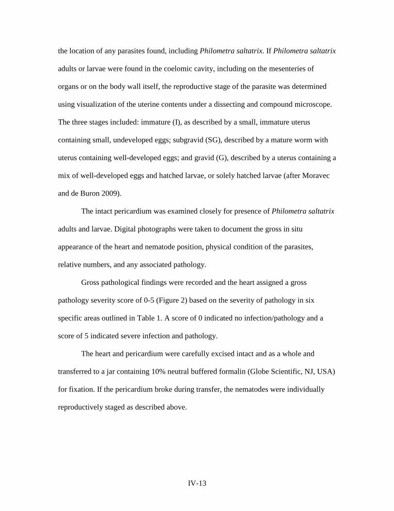
the location of any parasites found, including Philometra saltatrix. If Philometra saltatrix

adults or larvae were found in the coelomic cavity, including on the mesenteries of

organs or on the body wall itself, the reproductive stage of the parasite was determined

using visualization of the uterine contents under a dissecting and compound microscope.

The three stages included: immature (I), as described by a small, immature uterus

containing small, undeveloped eggs; subgravid (SG), described by a mature worm with

uterus containing well-developed eggs; and gravid (G), described by a uterus containing a

mix of well-developed eggs and hatched larvae, or solely hatched larvae (after Moravec

and de Buron 2009).

The intact pericardium was examined closely for presence of Philometra saltatrix

adults and larvae. Digital photographs were taken to document the gross in situ

appearance of the heart and nematode position, physical condition of the parasites,

relative numbers, and any associated pathology.

Gross pathological findings were recorded and the heart assigned a gross

pathology severity score of 0-5 (Figure 2) based on the severity of pathology in six

specific areas outlined in Table 1. A score of 0 indicated no infection/pathology and a

score of 5 indicated severe infection and pathology.

The heart and pericardium were carefully excised intact and as a whole and

transferred to a jar containing 10% neutral buffered formalin (Globe Scientific, NJ, USA)

for fixation. If the pericardium broke during transfer, the nematodes were individually

reproductively staged as described above.

IV-13

Grade 1 Grade 2 Grade 3 Grade 4 Grade 5 Inflammatory cell matrix

- Focal Multi-focal Multi-focal to diffuse

Diffuse

Pericardium color

Clear/transparent Slightly opaque

Slightly opaque to opaque

Multi-focally to diffusely opaque

Diffusely opaque

Pericardium texture

Smooth and thin Smooth Thickened, appears tacky

Thickened, rough

Thickened, rough

Adhesions between pericardium and body wall

- - +/- +/++ ++

Adhesions between epicardium and pericardium

- - + ++ +++

Condition of worms

None present Fresh or degenerate

Degenerate or embedded in matrix

Worms embedded in matrix

Worms embedded in matrix

Table 1. Pathological characteristics evaluated on gross dissection. + = 25% of surface area affected, ++ = 50% surface area affected, +++ = 75% surface area affected. Fresh worms are likely viable at time of collection and are not coated in inflammatory cell matrix. Degenerate worms are those that had died before collection and whose organs and cuticle are in various stages of physical deterioration. Worms embedded in inflammatory cells matrix are grossly visibly surrounded in a mixture of degenerate inflammatory cells, granulomatous inflammation, and cellular debris on histopathology.

Samples of liver and immature gonad were collected if the organs were not

grossly severely autolyzed. Carcasses were then eviscerated and reweighed. Viscera were

then re-examined for parasite adults and larvae. The body cavity was then flushed with

0.9% buffered saline solution and the flush solution caught in a Petri dish and examined

under the dissecting microscope for the presence of Philometra saltatrix larvae and

males. Any males or larvae found were quantified, photographed, and their location

recorded. Representative samples of males and larvae were saved in 95% ethanol or 10%

neutral buffered formalin for fixation.

Finally, otoliths were collected for future microstructure analysis and aging.

IV-14

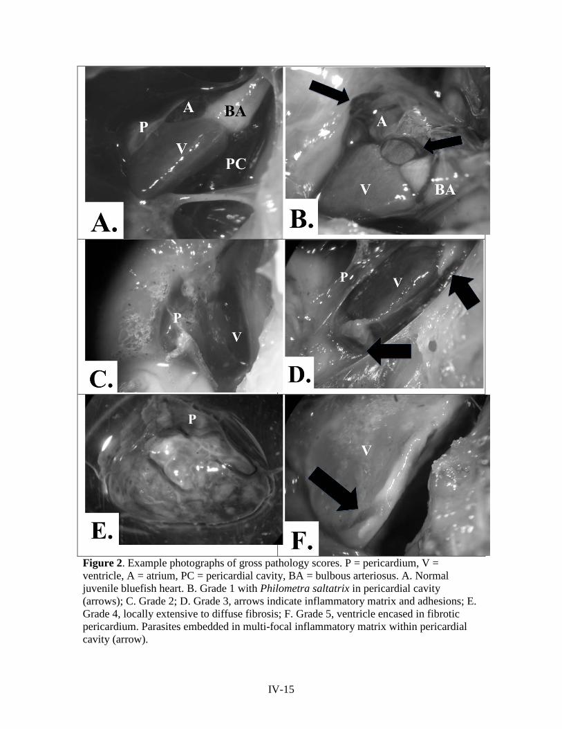
Figure 2. Example photographs of gross pathology scores. P = pericardium, V = ventricle, A = atrium, PC = pericardial cavity, BA = bulbous arteriosus. A. Normal juvenile bluefish heart. B. Grade 1 with Philometra saltatrix in pericardial cavity (arrows); C. Grade 2; D. Grade 3, arrows indicate inflammatory matrix and adhesions; E. Grade 4, locally extensive to diffuse fibrosis; F. Grade 5, ventricle encased in fibrotic pericardium. Parasites embedded in multi-focal inflammatory matrix within pericardial cavity (arrow).

IV-15

Histopathology

Formalin-fixed hearts were sectioned using a sectioning blade and included a

uniform section through the bulbous arteriosus, ventricle, and atrium. The sections were

placed in fine mesh tissue cassettes in 10% buffered formalin and submitted for

histological processing according to standard techniques and staining with hematoxylin

and eosin. Hearts were examined via high-power light field microscopy and pathological

findings and changes described for each sample. Slides with profound autolysis that

precluded accurate description of the cellular characteristics as well as those with

incomplete sectioning of all three heart divisions were omitted from histologic

assessment.

Slides were evaluated to assess severity and extent of inflammation, degree and

extent of pericardial fibrosis, physical condition of worms present in the pericardial

cavity, reproductive stages of worms present, and cellular character and extent of

inflammatory cell matrix present.

Histopathologic examination was used to confirm or amend the gross pathology

score assigned at initial dissection, based on the criteria above. The score that resulted

after any amendments was termed the Final Pathology Score (FPS). Final pathology

scores of grade four or five were determined to be of fatal severity based on the severity

and extent of pericardial fibrosis.

Slides of liver from both normal and pericardial cavity-infected fish were

submitted for processing as well as immature gonad samples.

IV-16

Data Analysis

Cohort assignment was accomplished by creating a length-frequency distribution

for each month sampled using R statistical software, and the distribution analyzed to

separate the fish into spring and summer-spawned cohorts by size.

Condition factor was calculated using the established formula:

K=weight in grams * 100

(fork length in cm)3

Infection in the pericardium was defined as the presence of any sex or stage

nematode in the pericardial cavity. Overall prevalence of pericardial infection was

defined as the number of fish from both cohorts, combined, with any sex or stage worm

present in the pericardial cavity divided by the total number of fish examined from both

cohorts combined. Prevalence of infection in the spring and summer-spawned cohorts

individually was defined by the number of fish infected in the pericardial cavity in the

cohort of interest divided by the total number of fish examined from the cohort of

interest.

The prevalence of pericardial cavity infection over time in a cohort was calculated

as the number of fish infected in the pericardium from the cohort of interest sampled

during a specific week period divided by the number of fish from the cohort of interest

sampled during that week period.

R statistical software was used for graphical representation of data and statistical

analysis. Fish fork length, condition factor, and mass were tested for normality using the

IV-17

Shapiro-Wilk normality test. Percent prevalence of infection, Final Pathology Scores

(FPS), and numbers of infected individuals between cohorts were compared using

Pearson's Chi-squared test with Yates' continuity correction. Means of non-normally

distributed data were analyzed non-parametrically using a Wilcoxon rank sum test with

continuity correction. A Welch Two Sample t-test was used to compare means among

normally distributed data. Spearman's rank correlation rho was used to assess correlation

between non-normally distributed numeric variables. A p value ≤ 0.05 was considered

significant in all tests.

Data was analyzed with both cohorts combined, and with cohorts individually

subsetted into spring and summer.

RESULTS

Cohort assignment

A total of 80 juvenile bluefish were processed. Fork lengths for all fish were not

normally distributed (Shapiro-Wilk normality test, W = 0.9672, p-value = 0.03742).

Length-frequency distribution analysis by month resulted in bimodal distributions with

two distinct length populations of juveniles representing the two cohorts. The mean fork

length (FL) for the spring cohort was 149.48mm (n=45) and 105.51mm (n=35) for the

summer cohort. Spring cohort fork length was normally distributed, while summer cohort

FL was not. A Wilcoxon rank sum test with continuity correction confirmed the

difference between the mean fork lengths of the cohorts was significant (W = 1427.5, p-

value = 5.531e-10).

IV-18

Prevalence

The overall prevalence of infection in the pericardium was 67.5% (54/80). While

the spring-spawned cohort prevalence of pericardial infection was 68.89% (31/45) and

the summer-spawned 65.71% (23/35), the difference in infection prevalence between

cohorts was not significant (Pearson's Chi-squared test with Yates' continuity correction,

X-squared = 0.0036, df = 1, p-value = 0.952). When looking at only infected fish,

35.48% (11/31) of the spring cohort and 39.13% (9/23) of the summer cohort had

potentially fatal infections. No significant difference in the number or percent prevalence

of fatal grade infections in infected fish existed between cohorts (Pearson's Chi-squared

test with Yates' continuity correction, p-value = 0.9916, p-value = 0.6984, respectively).

The percent prevalence of pericardial infection over time indicated that

prevalence increased in the spring cohort over mid-summer and declined to zero as the

spring cohort migrated out of the estuary (Figure 3). The spring cohort was no longer part

of samples collected after 9/27/2010. The summer cohort was first found in samples

beginning 8/2/2010. Infection prevalence was at 100% for the summer cohort when the

sampling period for the year ended on 10/25/2010.

IV-19

Figure 3. Weekly pericardial infection prevalence by cohort over sampling period.

A significant difference was observed in the mean fork length of fish infected in

the pericardium versus those not infected in the pericardium (Wilcoxon rank sum test

with continuity correction, p-value = 0.0004). Larger fish were more likely to be infected

in the pericardium, with a mean value of 140.65mm, versus those not infected

(mean=108.7mm FL). Only fish 97mm FL or larger were found infected in the

pericardium.

Fish infected in the pericardium also had a larger mean mass than those not

infected in the pericardium (Wilcoxon rank sum test with continuity correction, p-value =

0.0002).

0

20

40

60

80

100

120

7/25/06 8/25/06 9/25/06

Prev

alen

ce (%

)

Sampling date (week of)

Spring cohort, %Prevalence

Summer cohort, %Prevalence

IV-20

Pathology

Histopathologic examination supported the assigned Gross Pathology Score in

100% of cases and increased the pathology score in 12.12% (4/33) of cases. The revised

score resulting from the combination of Gross Pathology Score (GPS) with

histopathology, the Final Pathology Score (FPS) was used in further pathology analyses.

Prevalence of individual Final Pathology Scores are shown in Table 2. There was

no significant difference in either the percent prevalence or frequency of an FPS between

cohorts (Pearson's Chi-squared test with Yates' continuity correction, p-values = 0.1-

0.99).

Prevalence of Final Heart Pathology Scores in Juvenile Bluefish of the HRE Final Path Score

Spring cohort Prevalence (%)

Summer cohort Prevalence (%)

Both cohort

s Prevalenc

e (%) 0 14 31.11 12 34.29 26 32.5 1 8 17.78 8 22.86 16 20 2 9 20 4 11.43 13 16.25 3 3 6.67 2 5.71 5 6.25 4 5 11.11 4 11.43 9 11.25 5 6 13.33 5 14.29 11 13.75 n 45 100 35 100 80 100

Table 2. Prevalence of Final Heart Pathology scores in juvenile bluefish of the Hudson River Estuary. 0 = no infection present, 1 = mild pathology, 5 = most severe pathology.

With both cohorts combined, a significant positive correlation existed between

increasing fork length and increasing FPS (Spearman's rank correlation rho, p-value =

0.0010).

When the cohorts were examined individually, however, there was a strong

positive but barely non-significant correlation between increasing FL and FPS in the

spring-spawned cohort (p-value = 0.0898), but a strongly significant positive correlation

in the summer-spawned cohort (p-value = 3.957e-07). The positive correlation between

IV-21

increasing fork length and increasing Gross Pathology Score (GPS) was significant for

both cohorts combined and for the summer cohort, but barely non-significant for the

spring cohort alone (Spearman's rank correlation rho, both p-value = 0.0011; summer p-

value = 4.254e-07; spring p-value = 0.0565).

Overall prevalence of fatal infection (grades 4 and 5) was 25% (20/80) in juvenile

bluefish of the HRE during the 2010 sampling period. The average FPS for the spring and

summer cohorts were 1.89 and 1.80, respectively. No significant difference in the number

of fatal (grade 4 and 5) versus low-grade infections (grade 1 and 2) was observed

between cohorts (Pearson's Chi-squared test with Yates' continuity correction, X-squared

= 0.0018, df = 1, p-value = 0.9665). When looking at only infected fish, 35.48% (11/31)

of the spring cohort and 39.13% (9/23) of the summer cohort had potentially fatal

infections. The difference was not statistically significant (Pearson's Chi-squared test

with Yates' continuity correction, X-squared = 1e-04, df = 1, p-value = 0.9916).

A significant positive correlation existed between increasing FPS and collection

date later in the year for both cohorts combined and for the summer cohort alone

(Spearman's rank correlation rho, both p-value = 0.0080; summer p-value = 0.0012) but

not for the spring cohort (p-value = 0.1837). The FPS peaked for the spring cohort

between days 230-240 (mid to late August) and at day 270 (9/27/2010) for the summer

cohort. The peak refers to the time period with the greatest frequency of fatal severity

infections. Fatal severity infections were seen occasionally after the peak, but not with

equal frequency.

IV-22

Condition factor

Condition factor was normally distributed (Shapiro-Wilk normality test, W =

0.9945, p-value = 0.9834). Analysis of condition factor of fish infected in the heart versus

those not infected in heart revealed that infected fish have a higher condition factor than

those not infected in the heart. Or, alternatively, fish with a higher condition factor are

more often infected in the heart (Welch Two Sample t-test, p-value = 0.0015). When the

cohorts were examined individually, this was barely non-significant for the spring cohort

(normally distributed; p-value = 0.1403), and was very significant for the summer cohort

(not normally distributed; Spearman’s rank correlation rho, p-value = 3.779e-05). There

was no significant difference in the condition factor of fish with low-grade (grades 1 and

2) versus fatal grade (grades 4 and 5) infections (normally distributed; Welch Two

Sample t-test, p-value = 0.747). The mean condition factor of fish with fatal infections

was higher in the spring cohort than in the summer cohort (p-value = 0.0017). There was

no significant difference in the condition factor of those with low-grade infections

between cohorts (p-value = 0.2659).

Histopathology

Mild to moderate degrees of autolysis were present across all slides. Philometra

saltatrix females were often located at the base of the heart within the pericardial cavity,

wrapped around the bulbous arteriosus, which is a location associated with less cardiac

movement. This was also the most common site of inflammation and fibrosis. No

evidence was found of direct parasite damage to the cardiac musculature itself, nor any

evidence of myocardial invasion, attachment, pericardial rupture, or migration out of the

IV-23

pericardial cavity. Immature, subgravid, and gravid female worms were all found within

the pericardial cavity.

Grades 1-5 varied in the severity and extent of inflammation, pericardial fibrosis,

physical condition of the parasites, and extent of adhesions between the heart surface

(epicardium) and the pericardium, or the pericardium and the body wall. In both grade 4

and grade 5 infections, the epicardium and pericardium were diffusely affected, including

that of the ventricle, atrium, and bulbous arteriosus. The epicardium and pericardium

were, within the affected areas, fused and severely thickened (up to 3 mm) due to severe

mesothelial hyperplasia and hypertrophy, abundant granulomatous inflammation, and

immature fibrous connective tissue (Figure 4d, 4e). The epicardium had severe and

diffuse papilliferous projections of mesothelium, which were compressed and contained

few adult nematodes and occasionally, many larval nematodes.

Adult and larval nematodes were surrounded by many epithelioid to attenuated

macrophages, few admixed multinucleated giant cells, small to moderate amounts of

cellular debris, and moderate amounts of immature fibrous connective tissue. Gravid

females were most commonly represented, as well as some subgravid females. Adult

nematodes were often degenerate, with collapse and fragmentation of tissues, loss of

differential staining, and replacement of structures by cellular debris or rarely mineral.

Many larvae were located outside adult nematodes, embedded in granulomatous

inflammation (Figure 4f). These larvae were often degenerate, with collapse and

fragmentation of tissues, loss of internal structures with retention of a collapsed cuticle,

and loss of differential staining. Some larvae were found within the remains of adults,

IV-24

surrounded in granulomatous inflammation. The extent and thickness of fibrosis was

severe, often with involvement of tissues surrounding the bulbous arteriosus.

In contrast, low-grade infections (grade 1 or 2) were associated with non-

degenerate, recently viable parasites of all reproductive stages. These were not embedded

in inflammatory cell matrix and were associated with mild inflammation, which was

typically focal and restricted to the area immediately surrounding the parasite. Focal

areas of pericardial mesothelial hyperplasia were present. Grade two infections involved

a more reactive and thickened epicardium, with mild to moderate multi-focal

granulomatous inflammation.

The degree of pericardial thickening in grade three infections was considerably

increased compared to a grade two infection, with moderate to severe focal inflammation

and moderate focal to locally-extensive pericardial fibrosis. Subgravid and gravid worms

were seen embedded in a matrix of granulomatous inflammation. Parasites embedded in

matrix were often in various states of degeneration. Discrete areas of inflammatory

matrix were often associated with focal adhesions of the pericardium to the epicardium or

body wall.

Slides of liver sections were markedly autolyzed due to the freezing and thawing

process, and were not read. Slides of immature gonad were composed of moderately

autolyzed ovarian tissue containing primordial follicles.

IV-25

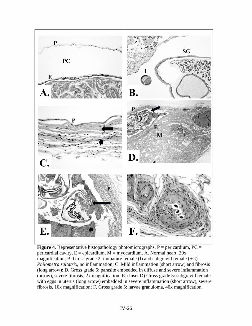
Figure 4. Representative histopathology photomicrographs. P = pericardium, PC = pericardial cavity, E = epicardium, M = myocardium. A. Normal heart, 20x magnification; B. Gross grade 2: immature female (I) and subgravid female (SG) Philometra saltatrix, no inflammation; C. Mild inflammation (short arrow) and fibrosis (long arrow); D. Gross grade 5: parasite embedded in diffuse and severe inflammation (arrow), severe fibrosis, 2x magnification; E. (Inset D) Gross grade 5: subgravid female with eggs in uterus (long arrow) embedded in severe inflammation (short arrow), severe fibrosis, 10x magnification; F. Gross grade 5: larvae granuloma, 40x magnification.

IV-26

DISCUSSION

Pathology and pathophysiology

While Philometra saltatrix is responsible for considerable fatalities in juvenile

bluefish, its effects are not due to direct tissue damage to the heart caused by the parasite.

The severe cardiac pathology is instead due to the host’s immune response to the dead

parasite and/or release of larvae into the pericardial cavity. This pathology is in the form

of varying degrees and extents of pericardial inflammation and fibrosis.

The heart of a fish is divided into three “chambers”: a single atrium, a single

ventricle, and the bulbous arteriosus (conus arteriosus). Blood from the hind end of the

fish is drained through the liver to the atrium, which then empties into the ventricle. The

ventricle, the muscular pump of the heart, pumps the blood forward to the gills for

oxygenation through a fibroelastic tube called the bulbous arteriosus. The pericardium

consists of two very thin layers. One layer, the visceral pericardium, is technically

adhered very closely to the surface of the heart and the second layer, the parietal

pericardium, makes up what is commonly known as the pericardium. The two layers

attach back together at the base of the heart around the bulbous arteriosus. The space

between these two layers is called the pericardial cavity. Normally, the parietal

pericardium is a single cell layer thick but tough (Figure 4a), and the pericardial cavity

contains a very small amount of clear, serous fluid, which acts as a lubricant (McGavin

and Zachary 2007).

IV-27

Histopathology

Histopathology served to further characterize the microscopic changes associated

with pericardial infection and understand the pathophysiology behind the changes

observed. Low-grade infections associated with live, non-degenerate worms induced

minimal pathology, and would not produce systemic signs of disease. Low-grade

infections were also associated with immature and subgravid female worms (Figure 4b).

The most severe pathology was associated with gravid worms that had died in the

pericardial cavity before or after releasing larvae into the pericardial cavity. Thus, the

majority of the inflammatory response happens after the worm dies or releases larvae.

The presence of macrophages, multi-nucleated giant cells, and cellular debris

indicates the inflammatory process seen is chronic in nature and directed at a large,

difficult to breakdown nidus of inflammation. Cellular debris indicates a longstanding

inflammatory response as well as bystander cell damage and cellular remodeling.

Granuloma formation, or the layering of fibrous connective tissue around an area of

inflammation, is a hallmark of chronic inflammation.

The presence of larval granulomas in some fish, or individual/clusters of larvae

surrounded by granulomatous inflammation, were observed both free in the pericardial

cavity indicating the release of larvae, and also within the degenerate cuticle of a dead

gravid female, indicating that the inflammatory response continued after the death of the

female (Figure 4f).

The matrix surrounding dead mature worms, formed by inflammatory cells and

cellular debris, anchored the pericardium to the epicardium frequently and facilitated the

organization of fibrosis and adhesions (Figure 4d).

IV-28

Pathophysiology

A fatal pericardial infection with Philometra saltatrix is defined by the severity

and extent of pericardial fibrosis present. Fibrosis is a natural response to chronic

infection and inflammation. A foreign body, such as a large nematode or nematode

larvae, which is incapable of being quickly broken down and cleared by the cells of the

immune system, elicits a demonstrated chain of responses from the body. These include

persistent active inflammation, tissue destruction, collagen deposition and fibrosis in an

attempt to repair tissue.

Early on, the response is mediated by certain types of white blood cells designed

for the chemical disintegration of foreign material. Over time, the predominant form of

white blood cell changes to those involved in the consumption and sequestration of

foreign material too large to be broken down. Chronic inflammation can be detrimental,

however. The long-term presence of inflammatory cells in an area, as well as their

chemical inflammatory mediators can cause damage to bystander tissues in the area. The

body tries to protect itself from damage by walling off the foreign object and laying down

connective tissue in the area to prevent further damage. It is important to note that

fibrosis, or the synthesis of collagen fibers leading to connective tissue formation is an

irreversible process. The degree and extent of the fibrosis, and how it affects nearby

tissues, is central to gauging if an infection will be fatal.

The transformation of the normal, thin, elastic, pliable pericardium to a thickened,

fibrous, inelastic pericardium due to chronic, severe inflammation can result in a

condition called constrictive pericarditis. As the fish grows or requires increased cardiac

IV-29

output, this inflexible pericardium restricts proper filling of the ventricle during diastole,

or the filling phase of the heart. While the prognosis for constrictive pericarditis in

mammals is generally poor (Asher and Klein 2002), the myocardium, or heart muscle

itself, is generally unaffected in these situations. Therefore, systolic function of the

ventricle is generally unaffected. Once the filling potential of the ventricle reaches its

filling constraint, however, filling ceases and congestion of blood behind the heart occurs

(Asher and Klein 2002).

Moderate to severe, or severe fibrosis of the pericardium, when diffuse, is

considered fatal based on inadequate ability of the heart to fill with blood during diastole.

Therefore, grade 4 or 5 infections, both grossly and histopathologically, are considered

fatal based on the degree and extent of pericardial fibrosis. Focal fibrosis is more

forgiving as the heart contracts and expands, and a fish with focal fibrosis of the

pericardium may be able to grow and function normally. Therefore, those fish with focal

fibrosis are not included in this calculation.

In mammals, constrictive pericarditis produces signs of exercise intolerance, poor

peripheral tissue perfusion, hepatic congestion, and eventual heart failure due to the

inability of the heart to meet the circulatory demands of the body. In fish, these changes

would be manifested as decreased ability to hunt and forage, decreased ability to pursue

normal migratory behavior, and increased susceptibility to predation. The effects would

become more pronounced as the fish outgrows the size and cardiac output of its confined

heart.

IV-30

Using histopathology as the definitive scoring tool, the prevalence of fatal

infection (grades 4 and 5) in all juvenile bluefish sampled from the HRE in 2010 was

25% (20/80). Of all infected fish, 37.04% (20/54) of infections were potentially fatal.

The 25% annual fatality rate is an approximation based on a relatively small

sample size from a portion of the year (late July to October). Ideally, fish should be

sampled over the entire calendar year sampling interval with a fixed number sampled

from each sampling location. Although the collection netting technique used was

designed to optimize random sampling of the fish population, one could argue this

fatality rate may be artificially increased due to the inability of clinically-affected grade 4

and 5 infected fish to escape sampling nets. However, the presence of uninfected/score-0

fish in the nets (see Table 2), as well as grades 1-3, makes this unlikely. Also, the peak

FPS occurred in mid to late August for the spring cohort and late September for the

summer, while sampling continued after those dates. A higher frequency of severe

infections would be expected at the end of the sampling period for both cohorts, along

with a relative decrease in the frequency of grade 0-3 of that cohort, if the prevalence of

clinically affected fish was increased. Instead, there is a decrease in the frequency of

severe pathology, indicating either resolving infections or the deaths of severely affected

individuals.

An important result of this study is the ability to employ a quick gross inspection

technique of pathology in the field with confidence in the agreement between GPS and

histopathology-verified FPS. There was always 100% agreement with the gross findings,

and histopathology is likely to support or increase the grade of severity. Thus, for

researchers assessing prevalence and severity of this infection in juvenile bluefish, it

IV-31

would not be necessary to submit individual histopathology samples to arrive at a

definitive severity grade. This means that the criteria included in the gross pathology

scoring system, which are designed to estimate the severity and extent of inflammation,

fibrosis, chronicity, and outcome, are also representative of the cellular changes.

The “grade 3” infection

Of the adjustments made to gross pathology scores, two grade one infections out

of 19 were increased to grade two, which is not surprising based on the small amount of

visible gross pathology. Also, two grade three infections out of seven were increased to

grade four. This is interesting because the degree of cellular change was more advanced

compared to the gross appearance. Yet, there were also grade three infections with a

similar gross appearance which were less severely affected on a microscopic level.

Across several of these grade three infections, a common finding involved degenerate

worms encased in inflammatory matrix. In the progression of infection from gross grade

one to grade five, the most severe inflammation and fibrosis is expected to be associated

with dead gravid females in grade five infections. After death, the worms begin to

degenerate and are removed slowly by the immune system.

However, in some grade three infections, the worms were degenerate and the

inflammatory response less severe and less extensive. This could indicate that some gross

grade three infections may be instead sequential to a grade five infection, reflecting a

state of resolving infection. This is supported by the presence of larval granulomas and

well-encapsulated degenerate worms, indicating a passage of time since the death of the

gravid female. Fibrosis of the pericardium was still present but focal to multi-focal in

IV-32

extent, which is expected because it is irreversible. Thus, both resolving infections of

non-fatal severity and progressing grade two infections could have the same gross grade

three pathology score, and would require histological examination. Progressing grade two

infections would involve live or very recently dead worms.

This sharing of grade 3 GPS by progressing and resolving infections is likely

responsible for the loss of significant positive correlation with increasing fork length and

increasing final pathology score in the spring cohort. The spring cohort is likely the only

cohort affected by this phenomenon because a longer window of the infection cycle is

seen during the sampling period, and the severe summer cohort infections have not yet

begun to resolve during the sampling period.

Parasite Ecology

Juvenile bluefish likely acquire the infection close to their spawning grounds

through the consumption of a copepod carrying an infective larva (Moravec 2004; Bryan

et al. 2008). Since a single adult arises from a single infective larva, multiple larvae are

acquired to result in multi-worm infections. The difference in the sexual maturity level

(immature, subgravid, or gravid) is a function of how recently the infective larva was

consumed (assuming a constant rate of parasite maturation). All females found in the

pericardial cavity were fertilized, indicating the presence of male nematodes in the fish’s

body as well. Recent research has shown males to be present in the body cavity and

gonad in juvenile bluefish (Koske et al., unpublished research).

The weekly percent prevalence of infection seen over the course of the sampling

period (Figure 3), which occurs in two major waves, reflects the staggered arrival of the

IV-33

cohorts in the estuary. After the fish acquires the parasite, at least two months pass before

infection is first visible in the pericardial cavity. For example, the summer cohort appears

in the HRE in early August but the first infection in the summer cohort is not found until

six weeks later, when prevalence suddenly approaches 100%. This is likely a function of

the close time proximity in which members of the summer cohort become infected and

the maturation time of the parasite. If the sampling period were extended earlier in the

year, a similar trend would likely be observed in the spring cohort.

Given the fact that the parasite’s reproductive strategy is likely linked to the off-

shore spawning of adult bluefish (Clarke et al. 2006; Moravec 2004) and the parasite is

likely acquired off-shore, not within the HRE, the parasite likely matures to its adult form

during the fish’s migration into, and early residence in, the estuary. This hypothesis is

supported by the fact that a significant trend exists linking increasing fork length with

increasing pathology score. If the parasite was acquired in the estuary, this trend would

be obscured by recurring waves of grade one infections and the progression of those

infections. Instead, there is a significant correlation in both cohorts with greater

pathology scores and larger fork lengths with collection dates later in the year. These

results point to a single infection event in each cohort. Also, evidence of re-infection,

defined by the co-existence of immature females and degenerate gravid females in the

pericardial cavity, was not observed during the entirety of this sampling period,

decreasing the likelihood the parasite is acquired in the HRE.

The overall prevalence of infection in the pericardium of all fish sampled was

67.5% (54/80). Studies evaluating the prevalence of parasitic infection in a natural wild

population are rare and thus comparable studies of other nematode parasites are few.

IV-34

With a prevalence of 67.5%, it is unusual to be lacking reports of occurrence from the

rest of the 1980s and 1990s. Cheung (1984) described an 80% prevalence in fish

examined at the New York Aquarium; however, his sample size was not reported in the

available abstract. Obviously, this parasite is widespread in the Hudson River estuary and

not localized to specific geographical areas of the Hudson River.

Importantly, during this sampling window, both the spring and summer cohorts

were equally infected in terms of prevalence and severity of infection. This indicates that

the summer cohort is not preferentially infected, and mortality associated with this

infection affects both cohorts equally. This is not in agreement with the proposition by

Clarke et al. (2006) who hypothesized that the summer cohort may be preferentially

infected due to a higher occurrence and intensity of Philometra saltatrix in the gonad of

summer-spawning adults.

Because the exit of the summer cohort from the HRE was not observed during the

sampling period, the summer cohort could possibly experience an increase in mortality

not seen in this study. However, it is also possible that the spring cohort experiences

mortality events as infection continues to progress when the fish have migrated back out

to sea and are effectively lost to the study. Thus, the ability to definitively evaluate and

compare mortality between cohorts in a natural setting may not exist. Experimental

infection and monitoring over time would give a better indication of mortality rates in

general, but the natural factors such as seasonal prey availability and water quality and

temperature that may affect infection rates between cohorts would be lost in this study.

During their residence in the HRE, juveniles grow in length, mass, and condition.

The smallest fish were not infected in the heart, and longer and heavier fish were more

IV-35

likely to be infected in the heart. This reflects the time interval between initial infection

and when the infection is grossly observable. Fish infected in the heart also had a higher

condition factor, which is not surprising given that condition factor is dependent on both

mass and length. Thus, the condition factor of the spring cohort is also expected to be

higher than for the summer because of their greater relative length and mass.

Gross pathology scores also increase with fork length, which reflects the fish

acquiring the parasite when small and having the infection develop and become more

severe as it grows over the course of the year. The fact that there is a trend for high

degree pathology in larger fish, in addition to the discovery that this correlates also with

time of year, is indicative that larger fish are not preferentially affected, but rather that the

score is the result of a natural long-standing infection. The final pathology score, which is

adjusted to reflect the histopathology findings, also increases with length and mass for the

same reason.

The histopathologic findings observed in 2010 juveniles of the HRE and larger

juveniles sampled from the New York Bight (NYB) in 2009 are similar (Koske and

Pinkerton 2010), although the prevalence of fatal infection in the NYB was only 9.09%.

This possibly reflects a further loss of severely infected individuals after migration out to

sea, or instead a reflection of the smaller sample size (n=33) in the NYB study.

In this sampling period, data on the spring cohort was collected for ten weeks, and

13 weeks for the summer cohort. However, of those 13 weeks, the summer cohort was

infected for only six weeks. The prevalence and average pathology score data were taken

from the entirety of the sampling period, not just the weeks where infection was present.

Thus, the comparison between the results of a 10-week and a 13-week study showed

IV-36

equal prevalence and pathology scores between cohorts. Without a sampling period that

includes both the arrivals and departures of both cohorts from the HRE, it cannot

definitively be said that one cohort is not preferentially affected over the other. However,

within the sampling period of this study, no significant difference was observed between

cohorts in the overall prevalence of pericardial infection, the prevalence of high versus

low-grade FPS, or the number or prevalence of fatal infections.

Condition factor and infection

Results showed that fish infected in the heart had higher condition factors than

those not infected in the heart. The formula used to calculate condition factor is

dependent on both fork length and mass. Since condition factor increases as fish FL

increases, the link between infection in the pericardium with both increased condition

factor and increased FL is not surprising. While one might expect a parasitized fish to

have a lower condition factor than a non-parasitized fish, the results show that fish are

grossly infected in the pericardium only after reaching 97mm FL and a condition factor

of 1.068. This could indicate two possibilities: 1) fish are infected early in life and

infection becomes apparent only around the age when condition factor approaches 1.0; 2)

the parasite might arrest in development within the fish until the fish reaches a size and

condition appropriate for optimal parasite development.

This also indicates that a severe pericardial infection does not induce significant

loss of condition while the fish resides in the estuary. Some loss of condition may be

present and not reflected here, however, because the increasing length of the fish would

mask any loss of mass due to the method of calculation. The fact that mass continues to

IV-37

increase with increasing FPS also indicates that infection does not significantly impact

fish mass. Generally, a parasite that routinely induced fatality or severe condition loss of

its host would not be evolutionarily successful due to host loss. Philometra saltatrix

infection may not even result in loss of condition. Knowing this infection can be fatal

through cardiac insufficiency and heart failure, any difference in condition may only

become apparent in severely infected fish just before the death of the fish, or not at all if

the fish succumbed to predation. These fatalities, of course, would occur out at sea and

are not measurable.

Suspected changes in the severely affected juvenile’s ability to successfully

forage, complete natural migrations, and escape predation are based on the

pathophysiology of heart failure. Moles (2003) described decreased prey capture rates in

Dolly Varden (Salvelinus malma) parasitized by the Philometrid nematode Philonema

agubernaculum in the body cavity. Parasitized fish captured only 32% of available prey

versus 64% by non-parasitized Dolly Varden. No difference was observed in the

condition of the parasitized versus non-parasitized Dolly Varden. Moles (2003)

hypothesized that while the effects of infection might be minimal when food supply is

abundant, in a limited food supply environment, the non-parasitized fish likely fare

better, and thus infection has the potential to alter predator-prey relationships.

Bluefish is a species heavily dependent on burst swimming and ambush during

normal feeding. Eventual decreased cardiac output and oxygenation of peripheral tissues

would lead to changes in cellular metabolism, thereby causing early muscle fatigue and

affecting foraging ability. Since constrictive pericarditis compromises the cardiac output

IV-38

of an affected fish, infection with Philometra saltatrix could also predispose affected fish

to fatalities associated with low dissolved oxygen content (McGladdery et al. 1988).

CONCLUSIONS

Pericardial cavity infection by Philometra saltatrix is an important source of

mortality in juveniles of the Hudson River Estuary, potentially fatal in 25% of all fish

sampled. The pathologic consequences of infection, which include varying degrees of

severity of constrictive pericarditis, have the potential over time to severely impact the

foraging and migration capabilities of severely affected growing fish. The most severe

pathology is induced after the death of the parasite and/or release of larvae into the

pericardial cavity. The severity of infection can be accurately assessed by quick gross

examination of changes seen in the character of the pericardium as described in this

study.

The results of this study show that both spring and summer-spawned cohorts are

equally affected in terms of prevalence of infection, severity of pathology, and prevalence

of fatal infections. Thus, this study suggests that Philometra saltatrix is not responsible

for the preferential decline in recruitment observed in the summer cohort.

Infection is likely acquired off-shore near spawning grounds and develops over

the course of the fish’s migration into the estuary. Over time, as the fish increases in size,

mass, and condition, the likelihood of infection in the pericardial cavity as well as the

severity of pathology increases. There was no evidence fish are re-infected in the estuary,

decreasing the likelihood of involvement of a paratenic host in transmission of the

infection in the estuary.

IV-39

RECOMMENDATIONS

Further study is needed to definitively quantify the negative effect on recruitment

caused by pericardial infection with Philometra saltatrix. Ideally, samples should be

collected from various locations in the HRE over the course of an entire calendar year in

order to observe the natural infection cycle in both cohorts.

Obtaining fresh samples of liver tissue at the time of processing could

histologically indicate whether passive congestion of blood is occurring in the liver of

grossly affected fish, which is a classic symptom of heart failure in mammals. This would

enable reliable extrapolation of other classic signs of heart failure to fish.

Optimally, in order to chronicle the story of infection from beginning to end and

note the timeline, as well as changes in health, growth rates, condition, and fecundity,

experimental infection should be pursued in a controlled environment over multiple

years. This would also enable the study of the health impacts on survivors of infection

and the whole of cohorts infected versus not infected.

Finally, it is important to note that the prevalence of infection likely varies from

year to year, depending on ocean current strengths, annual copepod crop, and water

temperature, as maturation rate of Philometrid species larvae in experimentally infected

copepods has been demonstrated to be heavily dependent on water temperature. Since the

presence of this parasite was not noted during the late 1980s and 1990s, it is possible that

infection prevalence has been steadily increasing since that time and Philometra saltatrix

infection in the pericardial cavity could be an already emergent and unmonitored source

of recruitment failure among juveniles of both cohorts. Fisheries biologists and

IV-40

conservation scientists should be involved in field monitoring of infection prevalence,

and additional effort should be directed toward elucidation of the life cycle of this

parasite to help direct future intervention.

IV-41

ACKNOWLEDGEMENTS

The authors would like to acknowledge the contributions of Dr. Timothy Yoshino

of the School of Veterinary Medicine, Director, Cellular and Molecular Parasitology

Training Program, University of Wisconsin-Madison for guidance on initial study design

and reproductive staging, and Dr. Marie Pinkerton, DVM, DACVP, Department of

Pathobiological Sciences, School of Veterinary Medicine, University of Wisconsin-

Madison for providing descriptive and diagnostic pathology services for the project along

with guidance on grading severity. We would also like to thank Amy Teffer, Department

of Environmental Conservation, UMass Amherst, for her assistance with statistical

analysis, and the New York State Department of Environmental Conservation for

sampling bluefish for the project. We would also like to thank Dr. František Moravec,

Institute of Parasitology, Biology Centre of the Academy of Sciences of the Czech

Republic, for his assistance confirming the identification of the parasite. Finally, David

Stormer, former Polgar fellow, Department of Environmental Conservation, UMass

Amherst, for his close guidance, instruction, and assistance with this project.

IV-42

LITERATURE CITED

Asher, C.R. and A.L. Klein. 2002. Diastolic heart failure: Restrictive cardiomyopathy,

constrictive pericarditis, and cardiac tamponade: Clinical and echocardiographic evaluation. Cardiology in Review. 10:4:218-299.

Beamish, R. and G. McFarlane (Eds.) 1989. Effects of ocean variability on recruitment

and an evaluation of parameters used in stock assessment models. Canadian Special Publication of Fisheries and Aquatic Sciences. 108.

Beyer, J.E. 1989. Recruitment stability and survival-simple size-specific theory with Examples from the early life dynamics of marine fish. Dana. 7:45-147.

Bryan, T.P., L.C. Tsoi, and I. de Buron. 2008. Development of the Philometrids

Philometra Overstreeti and Philometroides paralichthydis in the experimentally infected copepod Oithona colcarva. Folia Parasitologica. 55:313-315.

Burak, W.K. 2007. Infection of bluefish (Pomatomus saltatrix) ovaries by the

Drancunculoid nematode, Philometra saltatrix: prevalence, intensity, and effect on reproductive potential. Master’s thesis. Stony Brook University, Stony Brook, NY.

Cheung, P.J., R.F. Nigrelli, and G.D. Ruggieri. 1984. Philometra saltatrix infecting the heart of the 0 class bluefish, Pomatomus saltatrix (L.), from the New York coast. In S. F. Snieszko commemoration fish disease workshop, p. 27. Joint Workshop of Fish Health Section, AFS, and Midwest Disease Group, Little Rock, AR.

Clarke, L.M., A.D. M. Dove, and D.O. Conover. 2006. Prevalence, intensity, and effect

of a nematode (Philometra saltatrix) in the ovaries of bluefish (Pomatomus saltatrix). Fisheries Bulletin 104:118-124.

Conover, D.O., T. Gilmore, and S.B. Munch. 2003. Estimating the relative contribution

of spring and summer-spawned cohorts to the Atlantic coast bluefish stock. Transactions of the American Fisheries Society 132:1117–1124.

Chambers, R.C. and E.A. Trippel, (Eds.). 1997. Early Life History and Recruitment in

Fish Populations. Chapman & Hall, London. Hare, J.A., and R.K. Cowen. 1996. Transport mechanisms of bluefish (Pomatomus

Saltatrix larvae from South Atlantic Bight spawning grounds to Middle Atlantic Bight nursery habitats. Limnology and Oceanography. 41:1264-1280.

Hine, P.M., and C.D. Anderson. 1981. Diseases of the gonads and kidneys of New

IV-43

Zealand snapper, Chrysophrys auratus Forster (F. Sparidae). Pages 166-170 in M. E. Fowler, Editor. Wildlife diseases of the Pacific Basin and other countries. Academic Press, London.

Hjort, J. 1914. Fluctuations in the great fisheries of northern Europe viewed in the light of

biological research. Rapports et Proces-verbaux des Réunions. Conseil International pour l'Éxploration de la Mer . 20:1-228.

Houde, E.D. 1987. Fish early life dynamics and recruitment variability. American Fisheries Society Symposium. 2:17-29. Juanes, F., and D.O. Conover. 1995. Size-structured piscivory: advection and the linkage

between predator and prey recruitment in young-of-the-year bluefish. Marine Ecology Progress Services. 128: 287-304.

Juanes, F., J.A. Hare, and A.G. Miskiewicz. 1996. Comparing early life history strategies

of Pomatomus saltatrix: a global approach. Marine and Freshwater Research, 47:365-379.

Kendall, A.W. Jr., and L.A. Walford. 1979. Sources and distribution of bluefish,

Pomatomus saltatrix, larvae and juveniles off the east coast of the United States. Fisheries Bulletin. 77: 213-227.

Klein-MacPhee, G. 2002. Bluefish. Family Pomatomidae. Pages 400-406 in B.B.

Collette and G. Klein-MacPhee (Eds.). Bigelow and Schroeder’s Fishes of the Gulf of Maine Third Edition. Smithsonian Institution Press, Washington, D.C.

Koske, S.E. and M.E. Pinkerton. 2010. Pathology associated with pericardial

cavity infection by Philometra saltatrix (Nematoda, Philometridae) in juvenile bluefish (Pomatomus saltatrix). Poster session presented at: American College of Veterinary Pathologists Annual Meeting; 2010 October 30- November 3; Baltimore, Maryland.

Lassiter, R.R. 1962. Life history aspects of the bluefish, Pomatomus saltatrix (Linnaeus),

from the coast of North Carolina. M. Sc. thesis, North Carolina State College, Raleigh.

McGavin, M.D. and J.F. Zachary (Eds). 2007. Pathologic Basis of Veterinary Disease. Mosby/Elsevier, St. Louis. Fourth Edition. McGladdery, S.E., L. Murphy, B.D. Hicks, and S.K. Wagner. 1988. Pathology in Marine Science. pp. 305-315. London: Academic Press. Moles, A. 2003. Effect of Parasitism by Philonema agubernaculum (Nematoda: Philometridae) on the Ability of Dolly Varden to Capture

Prey in Fresh and Salt Water. Alaska Fishery Research Bulletin 10:2:119-123.

IV-44

Moravec, F. 2004. Some aspects of the taxonomy and biology of Dracunculoid nematodes parasitic in fishes: a review. Folia Parasitologica 51:1-13. Moravec, F. and I. De Buron. 2009. New data on three gonad-infecting species of

Philometra (Nematoda, Philometridae) from estuarine fishes in South Carolina, USA. Acta Parasitologica. 54:3:244-252.

Moravec, F., M. Magi, and F. Macchioni. 2008. Redescription of the

Gonad-infecting nematode Philometra saltatrix Ramachandran, 1973 (Philometridae) based on specimens from the type host Pomatomus saltatrix (L.) (Osteichthyes) from the Tuscan Sea, Italy. Folia Parasitologica 55:219-223.

Munch, S.B., and D.O. Conover. 2000. Recruitment dynamics of bluefish (Pomatomus

saltatrix) from Cape Hatteras to Cape Cod, 1973-1995. ICES Journal of Marine Science 57:393-402.

Oliva, M.E., A.S. Borquez, and A.N. Olivares. 1992. Sexual status of Paralabrax Humeralis (Serranidae ) and infection by Philometra sp. (Nematoda: Dracunculoidea). Journal of Fish Biology 40:979-980.

Olla, B.L., and A.L. Studholme. 1971. The effect of temperature on the activity of bluefish, Pomatomus saltatrix L. Biological Bulletin 141:337–349. Ramachandran, P. 1973. Philometra saltatrix sp n., infecting the gonads of the common

bluefish Pomatomus saltatrix (L.) off the New England coast of the United States. Zoologischer Anzeiger. 191:325-328.

Ramachandran, P. 1975. Philometra cephalus sp. N. infecting the gonads of the striped

mullet, Mugil cephalus L. from the Arabian Coast of Kerala, India, with a note on its pathology. Zoologischer Anzeiger. 191:140-144.

Rothschild, B.J. 1986. Dynamics of marine fish populations. Harvard University Press. Stormer, D.G., and F. Juanes. 2008. Cohort structure, growth, and energy dynamics of

Juvenile bluefish in the Hudson River estuary. Section VII: 26 pp. In S. H. Fernald, D. Yozzo and H. Andreyko (eds.), Final Reports of the Tibor T. Polgar Fellowship Program, 2008. Hudson River Foundation, New York, New York.

Sures, B. and K. Knopf. 2004b. Individual and combined effects of cadmium and

3,3’,4,4’,5 pentachlorobiphenyl (PBC 126) on the humoral immune response in European eel (Anguilla anguilla) experimentally infected with larvae of Anguillicola crassus (Nematoda). Parasitology 123: 179-184.

IV-45

DIET OF AMERICAN EEL (ANGUILLA ROSTRATA) ELVERS

IN A HUDSON RIVER TRIBUTARY


Leah M. Pitman

Polgar Fellow

Eckard College

St. Petersburg, FL 33711

Project Advisor:

Robert E. Schmidt

Bard College at Simon’s Rock

Great Barrington, MA 01230

Pitman, L.M. and R.E. Schmidt. 2012. Diet of American eel (Anguilla rostrata) elvers in a Hudson River tributary. Section V: 1-18 pp. In D.J. Yozzo, S.H. Fernald, and H. Andreyko (eds.), Final Reports of the Tibor T. Polgar Fellowship Program, 2011. Hudson River Foundation.

V-1

ABSTRACT

Elvers of American eel (Anguilla rostrata) were collected from the tidal mouth of

the Roeliff Jansen Kill, a Hudson River tributary. A total of 180 elvers collected from

June through early August 2011 were examined for gut contents. Five kinds of aquatic

insects comprised 94.9% of the total food items: four groups of chironomid midges

(Ablabesmyia sp., Pseudochironomus sp., Thienemanniella sp., and unidentified adult

midges) and an ephemeropteran (Caenis sp.).

The majority of the elvers were <9.0 cm TL and inhabited shallow (<10 cm deep)

gravel to cobble river margins. Comparison of gut contents to macroinvertebrates

collected by Surber sampling demonstrated that the elvers were non-selective, essentially

feeding at random on the most abundant benthic insects. Elvers were classified as

secondary or tertiary consumers in the detritus food web.

V-2

TABLE OF CONTENTS

Abstract ................................................................................................................... V-2

Table of Contents .................................................................................................... V-3

List of Figures and Tables....................................................................................... V-4

Introduction ............................................................................................................. V-5

Methods................................................................................................................... V-6

Results ..................................................................................................................... V-9

Discussion ............................................................................................................... V-14

Acknowledgments................................................................................................... V-16

Literature Cited ....................................................................................................... V-17

V-3


Figure 1. Oblique aerial view of the tidal mouth of the Roeliff Jansen Kill .......... V-7

Figure 2. Mean and range of total lengths of elvers .............................................. V-10

Figure 3. Length frequency of American eel elvers .............................................. V-11

Figure 4. Average number of food items per elver ................................................ V-12

Figure 5. Plot of the five food items that comprised 94.5% of the total ................ V-13

Table 1. Comparison of food items in elver stomachs with organisms from the Surber samples ......................................................................................... V-15

V-4

INTRODUCTION

The American eel is an important economic resource on the East Coast of the

United States. Recent evidence has indicated that the population of this species is

declining partially due to overfishing and habitat degradation (Haro et al. 2000);

therefore, it may be important to understand as much of the biology of American eel as

possible.

There have been several studies on the diet of the juvenile (yellow eel) stage of

American eel (e.g. Denoncourt and Stauffer 1993; Lookabaugh and Angermeir 1992;

Machut 2006; Wenner and Musick 1975). These studies uniformly concluded that small

yellow eels feed on benthic invertebrates (mostly insects) and larger (>35 cm) yellow eels

eat fishes and crayfishes. None of these studies looked at very small (<9 cm) eels.

Every spring thousands or tens of thousands of glass eels (4.5-7.0 cm) enter the

mouths of Hudson River tributaries (Schmidt and Lake, 2003, 2004, and unpublished

data). When reaching tributary mouths, they settle to the bottom, develop pigmentation

(at which point they are called “elvers”), and apparently stay in the shallow tidal habitat

for their first summer. Upstream migration is very slow (Haro and Krueger 1988).

Schmidt et al. (2009) reported very few of these elvers in an eel ladder 120 m upstream of

the tidal habitat (and up a waterfall) in the Saw Kill, Dutchess County.

The growth and survival of these small elvers determines the magnitude of the

upstream migration of yellow eels one to several years later. No studies have been done

on the diet of the newly settled elvers. Tesch (1977) said that glass eels don’t feed but

newly settled European eels (A. anguilla) fed on anything small enough to be ingested.

V-5

The purpose of this study was to document the diet of American eel elvers in the tidal

mouth of a Hudson River tributary.

METHODS

Study Area

This study was done in the tidal mouth of the Roeliff Jansen Kill, a Hudson River

tributary. The mouth of the Roeliff Jansen Kill is located in the town of Linlithgo,

Columbia County, NY. Specifically, samples were collected downstream (west) of the

Rt. 9G bridge (Figure 1). This study area was selected because previous experience

showed that elvers were numerous, the site is relatively easy to access, and few studies on

fishes have been done in the Roeliff Jansen Kill.

Field Procedures

Elvers were collected with a Smith-Root backpack electroshocker. Sampling was

conducted along the shoreline (usually north shore of the main channel) at or near low

tide until 20 individuals had been collected in any given trip. Elvers were over-

anaesthetized in clove oil and then transported to the laboratory.

Macroinvertebrates were sampled with a Surber sampler (330 µm mesh). Surber

sampling was done in the habitat where elvers were collected and triplicate samples were

taken on any one trip. Contents of the Surber sampler were preserved in 50%

isopropanol in the field and transported to the laboratory.

V-6

Figure 1. Oblique aerial view looking west at the tidal mouth of the Roeliff Jansen Kill, Columbia County, New York. The road is Rt. 9G. Most of the elver samples were taken from the shallow river margin indicated by the arrow and line. Figure is modified from a Google Earth photograph.

Laboratory Procedures

Elvers were measured (total length in cm) and then weighed on an electronic

balance (nearest 0.001 g). Specimens were then preserved in 70% ethanol. To determine

food habits, stomachs of elvers were removed and the contents were examined under a

dissecting microscope, identified initially to broad categories, and counted. Chironomid

V-7

midges were divided into “species” based on overall appearance (body color, size and

color of head, shape of head, size of prolegs, and size of antennae). Tentative

identification of chironomid midges to genus was done following Simpson and Bode

(1980) and Epler (2001). Other macroinvertebrates were identified using Wiggins (1977)

and Merritt and Cummins (1984).

Macroinvertebrates were sorted from the Surber samples under a dissecting

microscope. Specimens were sorted into the same categories established for the

organisms found in the elver guts.

Comparisons between the organisms in the elver guts and those collected with the

Surber sampler were done using Strauss’ (1979) linear index of food selection. This

index is expressed as: L = ri – pi, where L is the linear index, ri is the proportion of food

item “i” in the eels’ gut and pi is the proportion of food item “i” in the Surber samples.

The Index can have values between 1.0 and -1.0, the former indicating that eels are eating

only that food and it was not collected in the Surber samples and the latter indicating that

eels are not eating the only food item collected in the Surber samples. A score of “0”

would indicate that the proportion of food item “i” in the eels’ gut was the same as that in

the Surber samples– (i.e. no selectivity). Positive values (between 0-1) would indicate

that food item “i” was overrepresented in the eels’ guts compared to the Surber samples,

and thus purposefully selected. Negative values would indicate the opposite. Indices

were calculated by comparing each sampling trip to each Surber collection.

V-8

RESULTS

Nine sampling trips were made in this study from June 3 to August 5, 2011. Due

to some logistical problems, sampling events were not evenly spaced. The average size

of elvers collected was 58.3 mm total length (TL). Average size of elvers was expected

to increase over the summer, but there was little apparent change in average size per

collection (Figure 2). The median length category was 56-60 mm TL and the majority of

elvers were between 51-70 mm TL (Figure 3).

Out of 180 elvers examined, 26 of them contained no food (14.4%). A total of

631 food items were retrieved from elver stomachs, an average of 4.1 food items per

elver (that contained food) with a range of 1-17 items/elver. The food items were divided

into six categories: 1) Ablabesmyia sp., a Chironomidae (40.0% of the total food items,

average of 1.6/elver); 2) Pseudochironomus sp., a Chironomidae (7.9% of the total food

items, average of 0.4/elver); 3) Thienemanniella sp., a Chironomidae (31.2% of the total

food items, average of 1.4 items/elver); 4) unidentified adult Chironomidae (6.5% of the

total food items, average of 0.2/elver); 5) Ephemeroptera larva-Caenis sp. (8.9% of the

total food items, average of 0.4/elver); and 6) “other” (4.9% of the total food items,

average of 0.2 items/eel). The latter category included 12 chironomid pupae (in one

elver), 16 Trichoptera (14 Polycentropus sp. and 2 unidentified), 2 unidentified

Ephemeroptera, 1 Amphipoda, and 2 Gastropoda (Ferrissia sp.).

V-9

Date, 2011

Tota

l Len

gth

(mm

)

30

50

70

90

110

130

Jun 3 Jun 8 Jun 15 Jun 29 Jul 7 Jul 14 Jul 19 Jul 28 Aug 5

Figure 2. Mean (solid circle) and range (capped lines) of total lengths of elvers collected in the Roeliff Jansen Kill, summer 2011.

The range of elver sizes collected was 43-122 mm TL. Elvers were collected

from as wide a range as possible, but it is likely that some individuals were erroneously

included that were over a year old (and thus technically should be called “yellow eels”).

Individuals that were 90 mm or larger are very likely to be yellow eels (Machut 2006).

There was no evidence that these larger yellow eels consumed more prey items (Figure 4)

or different prey items (Figure 5) than the smaller elvers and therefore including them in

the analyses did not introduce a bias.

V-10

Total Length (mm)

Num

ber o

f Ind

ivid

uals

0

10

20

30

40

50

60

70

80

41-4

5

46-5

0

51-5

5

56-6

0

61-6

5

66-7

0

71-7

5

76-8

0

81-8

5

86-9

0

91-9

5

96-1

00

101-

105

106-

110

111-

115

116-

120

121-

125

Figure 3. Length frequency of American eel elvers collected in the Roeliff Jansen Kill, summer 2011.

The five food items that made up the majority of the diet were not necessarily

uniformly represented in each collection (Fig. 5). For instance, the larvae of the

chironomid, Thienemanniella sp., were bimodally distributed being most abundant in

mid-June and late July (Fig. 5). Larval Caenis sp., a small Ephemeroptera, was most

abundant in stomachs in mid-July, but were relatively rare in earlier and later samples. It

was presumed that these patterns reflect the life history of the insects in question.

The Surber sampler collections were done on June 9 and July 19, 2011. In the

June sample, 894 individuals were sorted (total of three replicates) that were classified

V-11

Figure 4. Average number of food items per elver or yellow eel plotted against average size of elver or yellow eel for each collection. The regression line indicates a slightly negative relationship (i.e.- larger eels eat fewer prey items) but the correlation coefficient is very low and the relationship is probably spurious.

into 15 groups (Table 1). The July collections contained many fewer individuals (total of

335) and were classified into 15 groups (Table 1). Strauss’ (1979) Linear Index of Food

Selection was calculated by comparing the proportion of each food item found in the

elvers’ stomachs (compared to the total number of all elvers) to the proportion of

organisms (out of the total) of each set of Surber samples (Table 1). There were seven

groups of organisms found in both the elver stomachs and the Surber samples. Although

some of the Index values were positive and some negative, all but one value was close to

zero (indicating no selection for or against each food item). The one exception was

Ablabesmyia sp. compared to the June Surber samples, which indicated a moderate

y = -1.0764x + 67.187R² = 0.1025

50

52

54

56

58

60

62

64

66

68

70

2 3 4 5 6 7

Aver

age

Tota

l Len

gth

(mm

)

Average Number of Food Items per Elver

V-12

Figure 5. Plot of the five food items that comprised 95% of the total food items in American eel elvers by collection date.

selection for this taxon (L = 20.1) in the eel’s diet. All of the invertebrate groups that

were represented in the Surber samples but not isolated from the eels were rare in the

Surber samples, and thus also had an Index value close to zero. It was concluded,

therefore, that American eel elvers are not feeding selectively, but rather taking food at

random. The proportions of food items in their stomachs closely reflects the abundance

of the food items in the environment.

0

10

20

30

40

50

60

Jun 3

Jun 8

Jun 15

Jun 29

Jul 7

Jul 14

Jul 19

Jul 28

Aug 8

Perc

ent o

f Tot

al

Date, 2011

Thienemanniella

Adult Midge

Caenis

Pseudochironomus

Ablabesmyia

V-13

DISCUSSION

The lack of food selectivity demonstrated in this study was similar to Tesch’s

(1977) statement that European eel (Anguilla anguilla) elvers consumed anything that

they could fit in their mouths. Since elvers are feeding non-selectively, the growth and

survival of individual elvers is determined solely by the quantity and quality of the

resources available.

The elvers should be considered as secondary or tertiary consumers in the detritus

food web. Both Pseudochironomus and Thienemanniella feed on detritus (McShaffrey

and Olive 1985), Ablabesmyia are obligate predators often feeding on other chironomids

(Roback 1985), and Caenis are widely considered omnivorous (Edmunds et al. 1976).

Growth of the elvers was expected over the study period. Instead (Fig. 2) little, if

any, change in size was seen over time. In fact, the elvers collected are essentially the

same size as the glass eels captured in Hudson River tributary mouths in April and May

(Schmidt and Lake 2003, 2004). If the elvers are not growing, or are growing so slowly

that it could not be detected, it raises the question of whether or not the food items

documented are adequate in quantity or quality. The possibility that the samples were

biased towards collecting only the smallest elvers was not eliminated. Elvers can be aged

by examining daily growth rings on otoliths (Martin 1995) but this was well outside the

scope of this study. The specimens were preserved in ethanol and are now catalogued in

the New York State Museum. These specimens could be aged and growth rates

calculated.

V-14

Table 1. Comparison of the proportion of food items in elver stomachs with the proportion of organisms from Surber samples. “L” is Strauss’ (1979) Linear Index of Food Selection where pi is the proportion of that food category in the Surber sample and ri is the proportion in the elver stomachs.

June Surber July Surber Food Category pi ri L pi ri L ___________________________________________________ Ablabesmyia .20 .40 .20 .32 .40 .08 Pseudochironomus .14 .09 -.05 .05 .09 .04 Thienemanniella .35 .33 -.02 .24 .33 .09 Caenis .08 .10 -.02 .15 .10 -.05 Adult Midge .14 .05 -.09 .02 .05 .03 Amphipoda .03 <.01 -.03 .04 .02 -.02 Ferrissia .01 <.01 -.01 .06 .03 -.03 Larval Elmidae .04 0 -.04 .06 0 -.06 Baetidae .03 0 -.03 .01 0 -.01 Caddisflies .02 0 -.02 Megaloptera .01 0 -.01 <.01 0 <-.01 Psephenidae .01 0 -.01 .01 0 -.01 Mite .01 0 -.01 Atherix .01 0 -.01 Midge pupa .01 0 -.01 Empedid fly <.01 0 <-.01 Adult Elmidae <.01 0 <-.01 Gerridae <.01 0 <-.01 Collembola <.01 0 <-.01 Isopoda <.01 0 <-.01 ____________________________________________________

Elvers were collected from the very shallow (<10 cm deep) margins of the Roeliff

Jansen Kill at or near low tide. In the instances when sampling took place in deeper

water, very few elvers were caught and a substantial numbers of larger yellow eels were

observed. Size segregation among habitats is known for American eel (Anderson and

Schmidt 2006) probably due to avoidance of aggressive and/or cannibalistic interactions

with larger eels (McCord 1977). Access to the sampling area is much more difficult at

high tides, and therefore sampling did not take place at those times. Elvers might in fact

V-15

be intertidal in this tributary, and therefore may spend much of their time burrowed into

dewatered sediments.

The Roeliff Jansen Kill is one of the larger tributaries to the Hudson River

estuary. The other 60+ tributaries vary considerably in size and physiography and few

have been examined to determine the distribution and habitat of American eel elvers.

The observations documented here are probably typical of most of the other Hudson

River estuary tributaries, but that is an untested hypothesis.

The elver stage of the American eel is one of several critical developmental stages

probably with a high mortality rate. Survivors are upstream migrant yellow eels whose

success determines the distribution and density of the population in a given tributary and

ultimately the abundance of downstream migrant silver eels. This study has documented

some aspects believed to be critical to the elvers in tidal water (foods and habitat) but

there needs to be much more work done on the tidal tributary habitat in the Hudson River

estuary.

ACKNOWLEDGMENTS

Haley Oller was invaluable to us in the field and in the laboratory, and we cannot

thank her enough. We appreciate the support we received from the Hudson River

Foundation and the assistance of Helena Andreyko, Dave Yozzo, and Sarah Fernald.

V-16

LITERATURE CITED

Anderson, J. and R. E. Schmidt. 2006. Significance of small impoundments to American eel (Anguilla rostrata). Section III: 20 pp. In W. C. Nieder and J. R. Waldman (eds.). Final Reports of the Tibor T. Polgar Fellowship Program, 2005. Hudson River Foundation, New York, New York.

Denoncourt, C. E. and J. R. Stauffer, Jr. 1993. Feeding selectivity of the American eel

Anguilla rostrata (LeSueur) in the upper Delaware River. American Midland Naturalist 129: 301-308.

Edmunds, G. F., Jr., S. L. Jensen, and L. Berner. 1976. The Mayflies of North and

Central America. University of Minnesota Press, Minneapolis. Epler, J. H. 2001. Identification manual for the larval Chironomidae (Diptera) of North

and South Carolina. Available online: http://h2o.enr.state.nc.us/esb/BAUwww/chiron_manual/intro.pdf Haro, A. and W. H. Krueger. 1988. Upstream migration and relative abundance of

elvers and young American eels (Anguilla rostrata (LeSueur)) in a Rhode Island stream. Canadian Journal of Zoology 66: 2528-2533.

Haro, A., W. Richkus, K. Whalen, A. Hoar, W. D. Busch, S. Lary, T. Brush and D.

Dixon. 2000. Population decline of the American eel: Implications for research and management. Fisheries 25: 7-16.

Lookabaugh, P. S. and P. L. Angermeir. 1992. Diet patterns of American eel, Anguilla

rostrata, in the James River drainage, Virginia. Journal of Freshwater Ecology 7: 425-434.

Machut, L. S. 2006. Population dynamics, Anguillicola crassus infection, and feeding

selectivity of American eel (Anguilla rostrata) in tributaries of the Hudson River, New York. MS Thesis, SUNY ESF.

Martin, M. H. 1995. Validation of daily growth increments in otoliths of Anguilla rostrata (Lesueur) elvers. Canadian Journal of Zoology 73: 208-211. McCord, J. W. 1977. Food habits and elver migration of American eel, Anguilla

rostrata (LeSueur), in Cooper River, South Carolina. MS Thesis. Clemson University, Clemson, South Carolina.

McShaffrey, D. and J. H. Olive. 1985. Ecology and distribution of chironomid larvae

from Carroll County, Ohio (Diptera: Chironomidae). Ohio Journal of Science 85: 190-198.

V-17

Merritt, R. W. and K. W. Cummins. 1984. An Introduction to the Aquatic Insects of North America. Kendall/Hunt Publishing Co., Dubuque, Iowa.

Roback, S. S. 1985. The immature chironomids of the Eastern United States VI.

Pentaneurini- genus Ablabesmyia. Proceedings of the Academy of Natural Sciences, Philadelphia 137: 153-212.

Schmidt, R. E. and T. R. Lake. 2003. Young of year American eel (Anguilla rostrata) In Hudson River tributaries: Year one. Report to Hudson River Estuary Program. Schmidt, R. E. and T. R. Lake. 2004. Young of year American eel (Anguilla rostrata) in Hudson River tributaries: Year two. Report to Hudson River Estuary Program. Schmidt, R. E., C. M. O’Reilly, and D. E. Miller. 2009. Observations of American eel

using an upland passage facility and the effects of passage on the population structure. North American Journal of Fisheries Management 29: 715-720.

Simpson, K. W. and R. W. Bode. 1980. Common larvae of Chironomidae (Diptera) from New York State streams and rivers. New York State Museum Bulletin 439. Strauss, R. E. 1979. Reliability estimates for Ivlev’s Electivity Index, the Forage Ratio,

and a proposed linear index of food selection. Transactions of the American Fisheries Society 108: 344-352.

Tesch, E. W. 1977. The Eel: Biology and Management of Anguillid Eels. Chapman and

Hall, London. Wenner, C. A. and J. A. Musick. 1975. Food habits and seasonal abundance of the

American eel, Anguilla rostrata, from the lower Chesapeake Bay. Chesapeake Science 16: 62-66.

Wiggins, G. B. 1977. Larvae of the North American Caddisfly Genera (Trichoptera). University of Toronto Press, Toronto.

V-18

GENOTYPING HISTORIC ATLANTIC TOMCOD SAMPLES TO DETERMINE

THE TIMELINE OF ONSET OF PCB RESISTANCE


Carrie E. Greenfield

Polgar Fellow

Department of Environmental Medicine New York University School of Medicine

Tuxedo, NY 10987

Project Advisor:

Isaac Wirgin Department of Environmental Medicine

New York University School of Medicine Tuxedo, NY 10987

Greenfield, C., and I. Wirgin. 2012. Genotyping Historic Atlantic Tomcod Samples to Determine the Timeline of Onset of PCB Resistance. Section VI: 1-26 pp. In, D.J. Yozzo, S.H. Fernald, and H. Andreyko (eds.), Final report of the Tibor T. Polgar Fellowship Program, 2011. Hudson River Foundation.

VI-1

ABSTRACT

It has been discovered that the contemporary population of Atlantic tomcod

(Microgadus tomcod) in the Hudson River has developed resistance to coplanar PCBs

and TCDD while populations of Atlantic tomcod from cleaner locales have not. The

mechanistic basis of this resistance has been traced to a single genetic polymorphism in

the aryl hydrocarbon receptor 2 (AHR2) gene. This variant polymorphism is a six base

pair deletion in the AHR2 locus and can be used as a DNA marker of the resistant

phenotype. This study was undertaken to determine if previous generations of tomcod in

the Hudson River were also resistant, in effect dating when this dramatic evolutionary

change took place. Between 1947 and 1977, approximately 1.3 million pounds of PCBs

were discharged into the Hudson River. It was hypothesized that tomcod collected in the

Hudson River from the 1930s would have a lower frequency of the variant AHR2 allele

(AHR2-1) compared to present day tomcod population. DNAs from fin clips of Hudson

River tomcod collected in 1936 and preserved in formalin were isolated using a modified

version of the Dayton Protocol. The isolated DNAs were PCR amplified at primers

specific to the AHR2 deletion polymorphism, digested with informative restriction

enzymes, and electrophoresed on agarose gels. A subset of the isolated DNAs was

successfully genotyped. It was determined that in the 1936 Hudson River tomcod

sample, the AHR2 deletion allele (AHR2-1) frequency was 38%. This frequency is

significantly less than in the current Hudson River population (96%). It was concluded

that PCBs probably contributed to the rapid evolutionary change that occurred in the

Hudson River tomcod population.

VI-2

TABLE OF CONTENTS

Abstract…………………………………………………………………….. VI-2

Table of Contents…………………………………………………………… VI-3

Lists of Figures and Tables…………………………………………………. VI-4

Introduction………………………………………………………………… VI-5

Methods…………………………………………………………………….. VI-14

Results……………………………………………………………………… VI-19

Discussion………………………………………………………………….. VI-23

Acknowledgements………………………………………………………… VI-25

Literature Cited…………………………………………………………….. VI-26

VI-3


Figure 1- Map of Hudson River……………………………………………. VI-6

Figure 2- Picture of Atlantic Tomcod……………………………………… VI-8

Figure 3- AHR Pathway …………………………………………………… VI-10

Figure 4- AHR Functional Domain………………………………………… VI-11

Figure 5- Contemporary AHR Allelic Frequencies in Tomcod…………….. VI-12

Figure 6- RFLP Assay………………………………………………………. VI-16

Figure 7- Agarose Gel Picture Using EcoNI Enzyme……………………… VI-19

Figure 8A/8B- Agarose Gel Picture Using MseI Enzyme………………… VI-20

Figure 9- Genotype Frequency Table…………………………………….. VI-22

Figure 10- Allelic Frequency Table………………………………………. VI-23

VI-4

INTRODUCTION

The Hudson River currently contains the largest federal Superfund site in the

United states (200 miles long) as a result of the release of 1.3 million pounds of PCBs

from two GE electrical capacitor manufacturing plants located at Fort Edward (RM195)

and Hudson Falls (RM 197) between 1947 and 1977 (Wirgin et al. 2011). PCBs are

highly lipophilic, very persistent in the environment, bioaccumulate and biomagnify

through the food chain. Atlantic tomcod Microgadus tomcod is a species of estuarine fish

found throughout the northeastern United States and Canada and have a high risk of PCB

exposure. This is because tomcod are bottom dwelling, feed on benthic invertebrate prey,

and have lipid rich livers. Additionally, tomcod are resident in their natural estuaries

year-round, increasing the likelihood of their exposure to industrial and municipal

pollutants that are often released into contaminated waterways. However, Atlantic

tomcod in the Hudson River have been found to show dramatic resistance to coplanar

PCBs and TCDD early life stage toxicities and cytochrome P4501A (CYP1A)

inducibility, while tomcod in cleaner estuaries such as the Miramichi River, New

Brunswick (NB), and Shinnecock Bay, New York (NY) do not exhibit resistance. The

mechanism of resistance is a six base pair deletion in the aryl hydrocarbon receptor 2

(AHR2) allele. Therefore, this variant allele (AHR2-1) serves as a marker of the resistant

phenotype. Since the PCBs were first introduced into the river in 1947, examining the

AHR2 allele frequencies in tomcod collected in the 1930s from the Hudson River may

determine if PCBs were the driving agent to this resistance.

VI-5

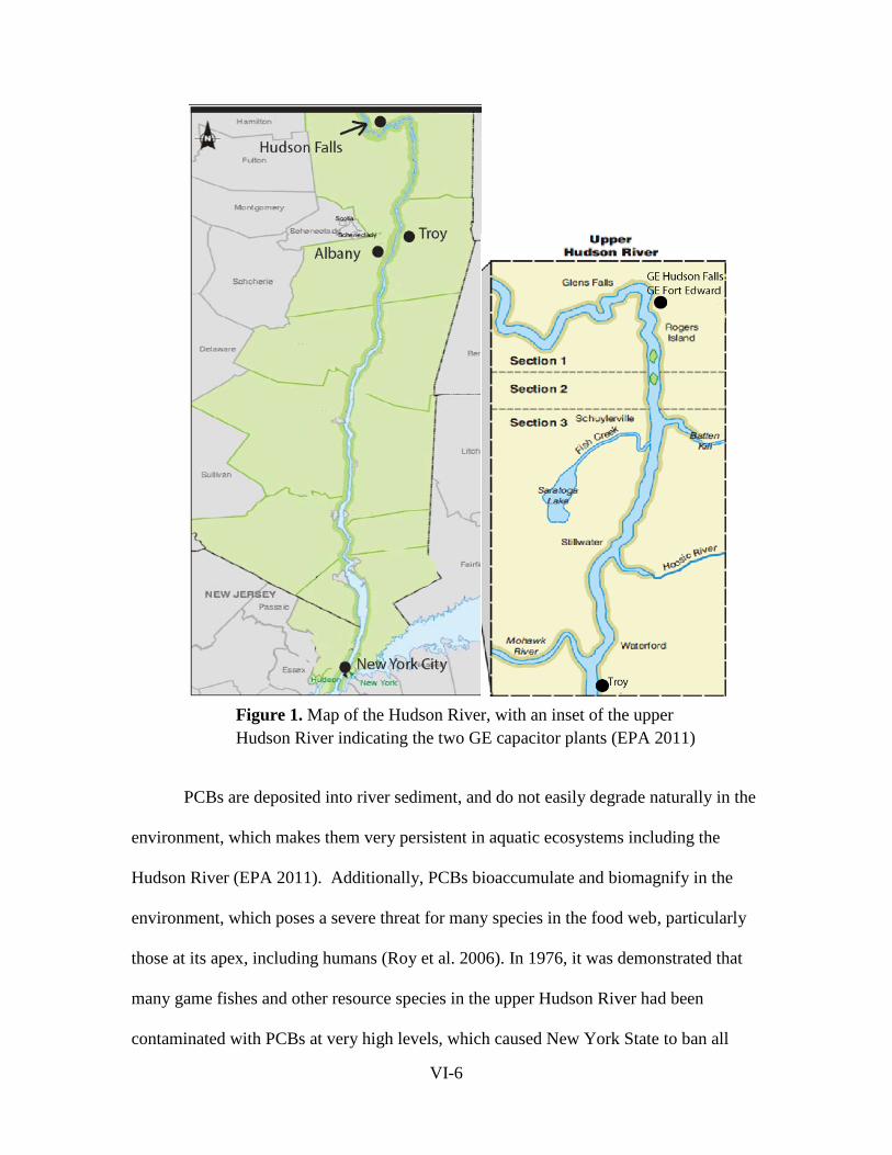
PCBs are deposited into river sediment, and do not easily degrade naturally in the

environment, which makes them very persistent in aquatic ecosystems including the

Hudson River (EPA 2011). Additionally, PCBs bioaccumulate and biomagnify in the

environment, which poses a severe threat for many species in the food web, particularly

those at its apex, including humans (Roy et al. 2006). In 1976, it was demonstrated that

many game fishes and other resource species in the upper Hudson River had been

contaminated with PCBs at very high levels, which caused New York State to ban all

Figure 1. Map of the Hudson River, with an inset of the upper Hudson River indicating the two GE capacitor plants (EPA 2011)

VI-6

fishing in the northern Hudson River and limit consumption of most fishes throughout the

estuary (EPA 2011). Bottom-dwelling fish species that are in direct contact with

contaminated sediments and feed on benthic invertebrates are especially susceptible to

PCB contamination as those are areas where PCB concentration is highest. Since PCBs

are not readily degraded by the environment, remediation efforts such as dredging to

remove PCBs are the most effective way to clean the river (EPA 2011). The first phase of

dredging PCBs in the Hudson River took place in a six mile area of the upper Hudson

River between May 15 and October 26, 2009. While this dredging successfully reached

the Environmental Protection Agency’s goal of removing ten percent of the

contamination, there is still a significant amount of PCBs remaining in the Hudson River

(EPA, 2011). The second phase of the dredging process began in May of 2011 and is

scheduled for continue for at least six years.

Atlantic tomcod (Microgadus tomcod) are distributed in rivers throughout the

northeast United States and Canada from north of the St. Lawrence River to the mouth of

the Hudson River (Wirgin and Waldman, 2004). The tomcod in the Hudson River are the

most southern spawning population of this species. Tomcod are estuarine, feed on small

benthic invertebrates, and known to be the only winter-spawning fish species in the

Hudson River (Yuan et al. 2006). Tomcod also have very lipid rich livers. This

combination of diet, habitat, and liver composition of Atlantic tomcod in the Hudson

River causes them to have an increased risk of exposure and bioaccumulation of PCBs

(Roy et al. 2006). Their unique ecological niche and wintertime spawning make their

young life stages critical prey in the Hudson River food web during the summer months

(Carlson et al. 2009).

VI-7

While PCBs are known to cause early life-stage toxicities in many fishes and

likely recruitment failure (Yuan et al. 2006), Atlantic tomcod in the Hudson River have

been found to show a dramatic resistance to PCBs and dioxin-induced early life stage

toxicities (Wirgin et al. 2011). In contrast, tomcod from cleaner locales are highly

sensitive to the early life stage toxicities of these chemicals (Roy et al. 2006). There are

usually tradeoffs to having this resistance, which can manifest as a significantly shorter

lifespan, higher sensitivity to other environmental stressors, and less competency in life

functions, such as reproduction (Yuan et al. 2006). It is thought that resistance is

associated with severe evolutionary costs, which would be selected against under normal

environmental circumstances (Wirgin et al. 2011). Therefore, as the Hudson River is

remediated and the PCB concentration is decreased, there may be a rapid evolutionary

shift in favor of non-PCB resistant tomcod.

Resistance to PCBs in the Hudson River tomcod population has been

demonstrated to result from a single genetic polymorphism in the aryl hydrocarbon

receptor (AHR2) (Wirgin, et al. 2011). This is the first identification of the mechanistic

Figure 2. Atlantic tomcod (Microgadus tomcod)

VI-8

basis of resistance to a toxicant in any vertebrate population and suggests that

contaminants have evoked rapid evolutionary change in the Hudson River tomcod

population by strong selection of a single variant gene at a single genetic locus. While

humans and other mammals have one AHR pathway (AHR1), fish and birds have two

AHRs (AHR1 and AHR2). In fish, binding efficiency assays have shown that AHR2

better binds TCDD and is likely more functionally active (Lin et al. 2001). The AHR

pathway regulates genes that encode xenobiotic metabolizing enzymes such as

cytochrome P4501A (CYP1A). Normally, when chemicals such as PCBs are present, this

signaling pathway is activated by ligand binding to the AHR receptor in the cytoplasm.

The bound complex travels to the nucleus, where it binds with aryl hydrocarbon receptor

nuclear translocator (ARNT). This three part complex works to bind to specific

recognition motifs, such as xenobiotic response element (XRE) and dioxin response

element (DRE) in the promoter of genes in the AHR battery. This in turn activates

transcription of dioxin responsive genes such a CYP1A (Roy et al. 2006). Most

importantly, it has also been shown that activation of the AHR pathway co-occurs with

the development of teratogenic effects in young life stages of fishes exposed to PCBs or

dioxins. Furthermore, AHR knockout models are no longer sensitive to PCB induced

early life stage toxicities confirming the essential role that AHR plays in mediating PCB

and dioxin toxicities (Prasch et al. 2003). Consistent with this role, tomcod with the AHR

polymorphism are no longer sensitive to PCB-induced early life stage toxicities or

induction of the cytochrome P4501A gene (Roy et al. 2006).

VI-9

One AHR2 polymorphism in tomcod is a six-base deletion downstream of the

ligand binding domain of the AHR2 and resistance is heritable by Hudson River tomcod

to at least the F2 generation (Wirgin et al. 2011). It was shown that the resistant AHR2

allele is at least five times less effective than the normal AHR2 allele (AHR2-2) in

binding TCDD (dioxin) and is significantly less able to drive reporter gene expression in

AHR deficient mammalian cells that were treated with graded doses of PCB126 or

TCDD(Wirgin et al. 2011). While there is nearly a

Figure 3. When PCBs are introduced, the AHR pathway is activated and the AHR complex translocates to the nucleus. In the nucleus, the HSP90 Dimer and XAP2 are lost, and ARNT binds to the complex. This allows the binding of dioxin response elements in the promoter of genes such as CYP1A. The complex then induces the transcription of dioxin response genes

VI-10

95% frequency of the AHR2 (AHR2-1) deletion variant allele in the Hudson River

tomcod population, there is a 5% or less frequency of the AHR2-1 variant allele in

Atlantic tomcod populations from other, nearby rivers. In previous studies, it was found

that in the Hudson River population, only heterozygotes had the normal AHR2-2 allele

and conversely, the AHR2-1 allele was only observed as heterozygotes in proximal

cleaner rivers (Romeo and Wirgin 2011). This suggests that both alleles existed in all of

the populations in the past in frequencies similar to what is seen today in the Miramichi

River and Shinnecock Bay (Wirgin et al. 2011), and that the pollution of the Hudson

River elicited a rapid evolutionary change in the tomcod population, leading to the

differing observed frequencies of this allele today. Due to this, the AHR2-1 allele was

considered a DNA marker of the resistant phenotype.

Figure 4. Functional domain of the AHR. A,B,and C show the three polymorphisms that all PCB-resistant fish have. “B” indicated the six base pair deletion

VI-11

The rate of evolutionary change at AHR2 and onset of when the Hudson River

tomcod population developed this resistance to PCBs is unknown. The goal of this

project was to use the AHR2 DNA marker to evaluate when resistance developed in the

Hudson River tomcod population. Originally, archived otoliths from tomcod collected

from the Hudson River in the 1980s were to be used; however, sufficient DNA could not

be obtained from these otoliths, so formalin-preserved fish collected in the 1930s from

the Hudson River were used instead. It was hypothesized that fish collected from the

Hudson River at earlier time points (prior to the release of PCBs) would have a reduced

frequency of the AHR2-1 variant compared to tomcod collected today. This would

support the notion that PCBs are the selective agents for the AHR2 variant, as well as

date the onset of PCB resistance by the Hudson River Atlantic tomcod population.

Figure 5. The current allelic frequencies of AHR2-1 and AHR2-2 in various tomcod populations in the northeastern United States and Canada.

VI-12

Additionally, understanding the timeline by which Hudson River population tomcod

became resistant to PCB toxicities can aid in the prediction and monitoring of the

frequency of the resistant phenotype as remediation of the Hudson River takes place.

Since PCB resistance may have evolutionary tradeoffs such as a truncated life span,

increased frequency of liver tumors, and decreased life functions, it is hypothesized that

resistance would be selected against as tomcod have reduced exposures to PCBs as a

result of remediation. Therefore, as the Hudson River becomes cleaner, this population

would quickly evolve to a genotype with a reduced frequency of the AHR2-1 variant for

resistance. Measuring population samples at periodic time points during remediation

would give a clear picture of the effectiveness that dredging is having on removing PCB

contamination from the Hudson River.

VI-13

METHODS

Sample Collection

Formalin-preserved tomcod samples collected in the 1930s from the Hudson

River were obtained from the collection of fishes housed at the New York State Museum

in Albany, NY. Hudson River fish had been collected from Orange, Rockland,

Westchester, and Dutchess counties in New York. Long island sound samples were

collected in Suffolk and Nassau counties in New York. Each fish’s pectoral fin was cut

and a 1-2mm section was placed into 95% ethanol. There were 110 fin clips collected

from Hudson River tomcod from 1936, and 60 fin clips collected from Long Island

Sound tomcod from 1938. These were taken back to the NYU laboratory for analysis.

DNA Isolation

To extract DNA from the formalin-preserved fin clips, a modified version of the

Dayton Protocol (Friedman and Desalle 2008) was used. This protocol calls for the fin

clips to be crosslinked in a Stratolinker (Stratogene, Santa Clara, CA), and then soaked in

a 1x GTE buffer (100 mM glycine, 10 mM Tris-HCL pH 8.0, 1mM-EDTA) for 72 hours.

This extended soaking was to disassociate the formalin from the tissue. After soaking,

the samples were air-dried, cut into small pieces, and homogenized. Proteinase K (15 µl)

was then added, and the samples incubated in a water bath at 50-55° C overnight. The

following day, a QIAGEN DNA kit was used to isolate the DNA. In this process,

RNAase and a protein precipitation solution were used to purify the DNA. An alcohol

precipitation process was then performed to form a DNA pellet, after which the pellet

was resuspended in DNA hydration solution. Each sample was read on a Nanodrop

VI-14

spectrophotometer at 260 and 280 nm to quantify their DNA concentrations and

determine their purity.

PCR and Restriction Enzyme Digestion

PCR and gel electrophoresis were performed to genotype DNAs from each

Hudson River historic sample and controls of contemporary Shinnecock Bay and Hudson

River DNAs. Isolated DNAs were added to a PCR master mix containing Taq DNA

polymerase enzyme. The primers that were used were 1401 (#78061722, 5’-

CACGCAGATCCAGACCAG-3’) and 1642 (#78061723, 5’

GCTCGCCCTCCTCCTTGA-3’) because the amplified segment of DNA (241 bp)

contains the six base deletion in AHR2. Additionally, primers 3376(#78061724,

5’CCTGCTGAAGACAACGAT-3’) and 3500 (#78061725, 5’-

GGGGTTTAAGGAGACGAT-3’) were used to analyze a downstream tyrosine to

asparagines (T:A) substitution polymorphism in the AHR2 that is coheritable with the six

base pair deletion. The PCR reactions were in 40 µl final volumes that contained 1 µl

DNA, 0.5mM of each primer (IDT, Coralville, Iowa), 0.008mM dNTP (GE Healthcare

Corp, Piscataway, New Jersey), 10x Taq Polymerase DNA buffer (Roche, Indianapolis,

Indiana), and 1 unit of Taq Polymerase (Roche, Indianapolis, Indiana). PCR reactions

were amplified in a thermocycler (MJ Research Inc, PTC-100) for 40 cycles. Each cycle

consisted of fifteen seconds at 95° C for denaturing, 15 seconds at 50° C for annealing,

and 30 seconds at 72° C for extension. After PCR, the samples were digested for one

hour using the restriction enzyme EcoNI (New England Biolabs, #B70045) for primer set

1401-1642 or enzyme MseI(New England Biolabs) for primer set 3376-3500. The EcoNI

enzyme is designed to cut the DNA at the six-base deletion site. When digested with

VI-15

EcoNiI if the site was missing (AHR2-1 alleles), the DNA was not cut and remained as

one large piece. If the site was present (AHR2-2 allele) the DNA was cut into two smaller

fragments.

However, when digesting with MseI, the opposite results would occur due to the

downstream polymorphism. Samples with the AHR2-1 variant allele would be digested,

while those with the AHR2-2 common allele would remain as one large piece. After

digestion, the samples were loaded into a 1.6% agarose gel and run for two hours. The

gel was then stained with ethidium bromide and visualized with UV light and imaged.

Figure 6. Agarose gel with tomcod DNA representative of variant AHR2 genotypes. DNAs were digested with EcoNI and electrophoresed in a 1.6% agarose gel. Lanes 1-7 indicate samples that were homozygote for the AHR2-1 variant allele, while lanes 8-14 indicate samples that were homozygote for the AHR2-2 common allele. Lane “M” indicated the marker to determine the size of the DNA bands.

VI-16

For each set of samples run on the gel, negative controls were included. These

were PCR blanks in which one well of the PCR plate contained the PCR master mix, but

no DNA was added. Ideally, these would show a clear lane with no bands. Occasionally,

a faint band would be present, and when this was the case only samples that were

significantly darker than this background could be reliably scored.

Data Analysis

AHR2 resistance genotypes can be determined based on the digestion pattern in

the gel. In tomcod that do not have the AHR2 deletion polymorphism (AHR2-2), the

DNA amplicon was cut into two smaller fragments (Figure 6). However, in those samples

where the AHR2 deletion was present (AHR2-1), the DNA remained as a single

fragment. Samples digested with MseI for the downstream base substitution would be

analyzed in the opposite way; tomcod samples with the AHR2-1 allele would be cut and

digested, while those without (AHR2-2) would remain as a larger piece. Since smaller

pieces run further on the gel, the samples which have the deletion, and therefore the

resistance could be determined.

Each sample was scored as a “1”, “2”, or “3” genotype for each of the two AHR2

polymorphisms. For EcoNI digested samples, “1” showed no digestion, indicating it is a

homozygote for the variant AHR2-1 genotype. A “2” showed complete digestion,

indicating that it was a homozygote for the common AHR2-2 genotype. A “3” had both

an undigested and digested band. This indicated that it was a heterozygote genotype, and

had one allele for each the variant and common allele. In the case of MseI digestions,

VI-17

samples were scored a “1” if they showed complete digestion, indicating that it was a

homozygote for the variant AHR2-1 genotype. A “2” score showed no digestion, and

corresponds to a homozygote for the common AHR2-2 genotype. A “3” score again was

a heterozygote with both bands present.

To determine the genotype frequency, the occurrence of each genotype number in

the archived samples was tallied, and these results were compared against the current

tomcod AHR2 genotype frequencies using a chi-squared test for independence. The

AHR2 allelic frequencies were then calculated from the genotype frequencies. Each

homozygote variant, or “1” score, contained two variant alleles, so the value for this

genotype was doubled. The amount of individuals scored under the “3” column were

added to this number because each of these fish contained one variant allele. The final

value is the frequency of the AHR2-1 variant allele. For the homozygote common allele

frequencies, the same procedure was done except that “2” score was doubled, and the “3”

score was added to it. Another chi-squared test for independence was performed to

compare the AHR2-2 allelic frequencies in the archived and contemporary Hudson River

samples. Differences in genotype and allelic frequencies were considered statistically

significant when p < 0.05.

VI-18

RESULTS

In order for a sample to be considered reliable, it had to be PCR amplified and

clearly analyzed three separate times. From the 110 Hudson River samples extracted and

analyzed, 20 samples were successful. The results from these tomcod specimens were

then used to perform the statistical analysis.

Gel Pictures

All of the tomcod analyzed were PCR amplified and digested in triplicate, both

with 1419-1668 primers (EcoNI digestion) and 3376-3500 primers (MseI digestion). The

gel pictures showed clear positive and negative controls, which allowed for the

characterization of the archival samples. The samples (as shown in Figures 8A and 8B in

Figure 7. Agarose gel picture of tomcod DNA after PCR amplification for an AHR2 amplicon and digestion with EcoNI enzyme. The positive and negative controls are highlighted.

VI-19

dark lettering) were then scored using the “1”,”2”, “3” designations for homozygote

variant, homozygote common, or heterozygote genotype, respectively.

Figure 8A and 8B. Agarose pictures of tomcod DNAs digested with MseI restriction enzyme. Controls, markers, and successfully analyzed samples are indicated in dark lettering. White lettering indicates samples that did not successfully amplify or genotype. The “blank” lanes are PCR water blanks. These are lanes in which the PCR mixture was amplified without any DNA

VI-20

AHR2 Genotype Frequencies

The genotype frequencies represent the number of individuals which exhibit each

genotype. From this data, it can be determined that the genetic frequency of the

homozygote PCB-resistant genotype, AHR2-1, in Hudson River tomcod collected in

1936 was 2, which is approximately 10% of the samples. This is in comparison to the

present day population, which has a frequency of 93%, for the AHR2-1 genotype. Also of

note is that the difference in the number of heterozygotes between each time point: 55%

(11 of 20) of the specimens from 1936 had this genotype, while only about 7% (4 of 54)

from the present day possess it. A chi-squared test to compare the 1936 Hudson River

tomcod population genotypes to the present day Hudson River population showed a

highly significant p-value ( < 0.0001).

VI-21

Allelic Frequencies

Additionally, frequencies of the variant AHR2-1 allele and the common AHR2-2

allele were calculated for the archived and contemporary Hudson River tomcod samples

and statistically compared. This was done using the genotypes determined from the

agarose gel pictures. In tomcod collected from the Hudson River in the 1930s the AHR2-

1 allele frequency was 15 of 40, which was 37%. The allelic frequency of the variant

AHR2-1 allele in present day tomcod from the Hudson River is 104 of 108, or 96%. A

chi-squared test was done to compare the statistical significance of AHR2 allele

frequency for the tomcod from 1936 and present day, resulting in a p-value of <0.0001.

Figure 9. AHR2 genotype frequencies in contemporary and archived Hudson River tomcod samples.

VI-22

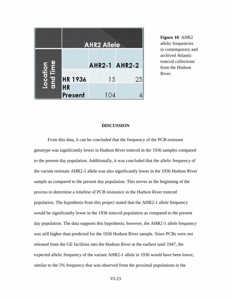
DISCUSSION

From this data, it can be concluded that the frequency of the PCB-resistant

genotype was significantly lower in Hudson River tomcod in the 1936 samples compared

to the present day population. Additionally, it was concluded that the allelic frequency of

the variant resistant AHR2-1 allele was also significantly lower in the 1936 Hudson River

sample as compared to the present day population. This serves as the beginning of the

process to determine a timeline of PCB resistance in the Hudson River tomcod

population. The hypothesis from this project stated that the AHR2-1 allele frequency

would be significantly lower in the 1936 tomcod population as compared to the present

day population. The data supports this hypothesis; however, the AHR2-1 allele frequency

was still higher than predicted for the 1936 Hudson River sample. Since PCBs were not

released from the GE facilities into the Hudson River at the earliest until 1947, the

expected allelic frequency of the variant AHR2-1 allele in 1936 would have been lower,

similar to the 5% frequency that was observed from the proximal populations in the

Figure 10. AHR2 allelic frequencies in contemporary and archived Atlantic tomcod collections from the Hudson River.

VI-23

relatively clean Niantic River, CT., and Shinnecock Bay NY. (Wirgin et al. 2011). This

would lead to the conclusion that while PCBs were not the sole driving force for this

resistance, their introduction in the Hudson River ecosystem probably played an

important role in the rapid evolution seen in the tomcod population in the past eighty

years. Alternatively, it is possible that the frequency of AHR2-1 was historically higher

than seen in the other two nearby tomcod populations. With the current data, it is not

possible to distinguish between the two possibilities.

However, there were limitations to this study. The archived tomcod samples were

preserved in formalin, which made the DNA extracting process much longer and more

difficult than for contemporary samples. The longer extraction time limited the number of

samples from which DNA could be isolated and the success of their analysis. Some of the

samples that were not isolated included reference ones collected from the Long Island

Sound in 1938. Their genotypes would have provided an excellent positive control for

this study. Due to this, not all of the samples extracted were able to provide adequate

DNA to be PCR amplified.

Further research involves continuing to isolate and analyze DNA from additional

archived Hudson River specimens to expand the sample size which will increase the

statistical power in comparing the AHR2 genotype and allelic frequencies in archived

versus contemporary Hudson River tomcod collections. Also, this work would include

replicating the current samples that did not amplify multiple times to obtain a larger

sample size. It will also be important to genotype archived samples collected from the

Long Island Sound in the 1930s that were not available for this report. Additional

research would be to genotype Hudson River tomcod collected at various time points

VI-24

during the period of 1947 to the present day. Having the allelic frequencies of Hudson

River Atlantic tomcod populations throughout the release of PCBs (1947-1977) as well as

after the plants were closed and then when remediation began (2009) would provide a

clear timeline of the resistance to PCBs in these fish.

ACKNOWLEDGEMENTS

I would like to thank Dr. Isaac Wirgin for being the project supervisor as well as

for his advice and support during this project, as well as Dr. Nirmal Roy for his enormous

amount of help to isolate and PCR the DNA. I would also like to thank the other

members of Dr. Wirgin’s lab, Diane Curry and Lorraine Maceda for their support in the

laboratory. Additionally, I would like to acknowledge Dr. Robert Daniels and The New

York State Museum, who supplied the archived samples. Lastly, I would like to thank the

Hudson River Foundation for the funding and support for this project.

VI-25

REFERENCES

Carlson, E. A., N.K Roy, and I.I. Wirgin. 2009. Microarray analysis of polychlorinated biphenyl mixture-induced changes in gene expression among Atlantic tomcod populations displaying differential sensitivity to halogenated aromatic hydrocarbons. Environmental Toxicology and Chemistry 28: 759-771.

EPA. 2011. Hudson River PCBs. Retrieved 1/26, 2011, from http://www.epa.gov/hudson/

Friedman, M. and R. Desalle. 2008. Mitochondrial DNA extraction and sequencing of formalin-fixed archival snake tissue. Mitochondrial DNA 19: 433-437.

Lin, T., K. Ko, R.W. Moore, D.L Buchanan, P.S. Cooke, and R.E. Peterson. 2001. Role of the aryl hydrocarbon receptor in the development of control and 2,3,7,8-tetrachlorodibenzo-p-dioxin-exposed male mice. Journal of Toxicological and Environmental Health 64:: 327-342.

Prasch, A. L., T. Hiroki, S.A Carney, D. Wu, H. Takeo, and R.E Peterson. 2003. Aryl hydrocarbon receptor 2 mediates 2,3,7,8-tetrachlorodibenzo-p-dioxin developmental toxicity in zebrafish. Toxicological Sciences 76: 138-150.

Romeo, M. and I. Wirgin. 2011. Biotransformation of organic contaminants and the acquisition of resistance. pp. 176-208 In: C. Amiard-Triquet, P.S. Rainbow and M. Romeo (Eds.), Tolerance to Environmental Contaminants. Boca Raton, FL: CRC Press

Roy, N. K., S.C.,Courtenay, R.C., Chambers, and I.I., Wirgin. 2006. Characterization of the aryl hydrocarbon receptor repressor and a comparison of its expression in Atlantic tomcod from resistant and sensitive populations, Environmental Toxicology & Chemistry 25: 560-571.

Wirgin, I., N.K.,Roy, M. Loftus., R.C. Chambers., D.G. Franks., and M.E. Hahn. 2011. Mechanistic basis of resistance to PCBs in Atlantic tomcod from the Hudson River. Science 331: 1322-1325.

Wirgin I. and J.R. Waldman. 2004. Resistance to contaminants in North American fish populations. Mutation Research/Fundamental and Molecular Mechanisms of Mutagenesis 552: 73-100.

Yuan, Z., S. Courtenay, and I.,Wirgin. 2006. Comparison of hepatic and extra hepatic induction of cytochrome P4501A by graded doses of aryl hydrocarbon receptor agonists in Atlantic tomcod from two populations. Aquatic Toxicology 76: 306-320.

VI-26

http://www.epa.gov/hudson/

PILOT STUDY FOR LASER ABLATION AND STABLE ISOTOPE ANALYSIS OF FEATHERS, EGGSHELLS AND PREY OF GREAT BLUE HERONS

SAMPLED ACROSS AN URBANIZATION GRADIENT IN THE MID-HUDSON RIVER VALLEY


Jill K. Mandel

Polgar Fellow

Department of Environmental and Forest Biology

State University of New York College of Environmental Science and Forestry

Syracuse, NY 13210

Project Advisor

Karin E. Limburg

Department of Environmental and Forest Biology

State University of New York College of Environmental Science and Forestry

Syracuse, NY 13210

Mandel, J.K., and K.E. Limburg. 2012. Pilot Study for Laser Ablation and Stable Isotope Analysis of Feathers, Eggshells and Prey of Great Blue Herons Sampled Across an Urbanization Gradient in the Mid-Hudson River Valley. Section VII: 1-31 pp. In D.J. Yozzo, S.H. Fernald, and H. Andreyko (eds.), Final Reports of the Tibor T. Polgar Fellowship Program, 2011. Hudson River Foundation.

VII - 1

ABSTRACT

The need to trace pollutants, especially heavy metals like lead and cadmium, and

human-derived organics like prescription drugs, personal care compounds and stimulants,

through aquatic ecosystems is an area of increasing concern. This study tested whether

laser-ablation inductively-coupled plasma mass spectrometry (LA-ICP-MS) and stable

nitrogen isotope analysis can be used to trace uptake and bioaccumulation of these

potentially harmful chemical compounds in the Hudson River system. Five colonies of

great blue herons (Ardea herodias) in the mid-Hudson River valley were observed during

the nesting season of 2011. Once the nests were abandoned at the end of the season,

chick feathers, chick bones and discarded prey items were collected for chemical

analyses. It was hypothesized that items from colonies in more urbanized areas would

contain more trace metal and sewage contamination than colonies in more rural areas,

and that the higher levels of contamination would have an effect on reproduction and

recruitment of top-level predators such as the great blue heron. Due to small sample

sizes, strong conclusions could not be drawn, but the results of the LA-ICP-MS analysis

indicate that trace metal uptake and bioaccumulation is more complicated than the

general hypothesis assumed. The concentrations of strontium in heron feathers increased

with increasing urbanization, but the manganese and zinc concentrations decreased, and

copper concentrations remained the same across the urbanization gradient. The stable

isotope results indicated that multiple food webs with varying trophic levels exist in the

mid-Hudson area. No difference was found in fledgling success between the five nest

sites. Further studies with more specific expectations are recommended in order to

determine the roles of industrial and sewage pollution in the Hudson River ecosystem.

VII - 2

TABLE OF CONTENTS

Abstract ........................................................................................................................ VII-2

Table of Contents ......................................................................................................... VII-3

List of Figures and Tables............................................................................................ VII-4

Introduction .................................................................................................................. VII-5

Methods...................................................................................................................... VII-11

Nest observations and sample collections.............................................................. VII-11

Observational data analysis.................................................................................... VII-12

Trace metal analysis ............................................................................................... VII-14

Stable isotope analysis ........................................................................................... VII-15

Results ........................................................................................................................ VII-16

Observational results .............................................................................................. VII-16

Trace metal results ................................................................................................. VII-17

Stable isotope results.............................................................................................. VII-20

Discussion .................................................................................................................. VII-22

Acknowledgements .................................................................................................... VII-28

Literature Cited .......................................................................................................... VII-29

VII - 3

LIST OF FIGURES AND TABLES Figure 1: Heron observation sites and estimated parent foraging radii ..................... VII-13

Figure 2: Example results from LA-ICPMS analysis ................................................ VII-19

Figure 3: Scatterplot of mean stable isotope values for individual feathers. ............. VII-22

Table 1: Results of heron nest observations .............................................................. VII-16

Table 2: Summarized LA-ICPMS results for feathers and eggshells. ....................... VII-19

Table 3: Summary of LA-ICPMS results of heron chick bone and prey items ......... VII-20

Table 4: Mean stable isotope values for feathers collected at the Lower Hook and Orange

Lake sites ....................................................................................................... VII-21

VII - 4

INTRODUCTION

The Hudson River has been a dumping ground for human-derived pollutants since

before the Industrial Revolution. In 1984, the Environmental Protection Agency (EPA)

declared the Hudson River a 200-mile long Superfund site, and several dredging projects

are currently under way (EPA 2011). While these dredging projects have been successful

in cleaning up much of the contamination in the river, these projects have focused

primarily on removing organic industrial contaminants, like PCBs, so some potentially

toxic trace metals like cadmium (Cd), manganese (Mn) and lead (Pb) may remain in the

system. At the same time, antiquated sewer systems and high population density

continue to confound efforts to clean up wastewater pollution throughout the watershed.

Repeated, chronic overflows of wastewater treatment plants and municipal sewer lines

have introduced increasing amounts of human-derived exotic organic chemicals, such as

prescription drugs, personal care substances and stimulants, into the Hudson River.

Uptake of these heavy metals and exotic chemicals by local food webs and their long-

term effects on the organisms is of great concern and still under investigation (Comeau et

al. 2008; Fent et al. 2006; Wilson et al. 2003; Wilson et al. 2008).

Continuing population and economic growth makes finding resolutions to

pollution issues difficult. The urban sprawl phenomenon has extended major population

centers further and further into natural habitats, and the usual precursor to settlement is

road-building. As discussed by Forman and Deblinger (2000), roads themselves can have

significant effects on the ecology of the surrounding area, from car-wildlife interactions

to the spread of exotic species to rapid runoff input to local waterways. Once the roads

VII - 5

are established, the rest of the required infrastructure for human habitation, like municipal

water supplies or drilled wells and sewer lines or septic systems, follows. This additional

infrastructure can exacerbate urbanization's effect on local waterways, and as a result, the

presence of roadways in an area can provide a clue as to the health of the area's

waterways. In fact, the road density of an area is often well-correlated with other

measures of human activity in an area, and has been used in ecological studies to study

the effect of urbanization on the natural world (National Research Council 2008).

The Hudson River Estuary is home to a rich variety of estuarine dependent

avifauna including bald eagles (Haliaeetus leucocephalus), osprey (Pandion haliaetus),

and great blue herons (Ardea herodias). Great blue herons are primarily piscivorous top-

level predators, but they have been known to take salamanders, turtles, crabs, voles, and

even other birds (Vennesland and Butler 2011). Adult herons usually feed in marshes

and along riverbanks, and heron chicks derive their nutrition exclusively from parental

regurgitation. Therefore, heron chicks may be especially sensitive to pollutants that

bioaccumulate in aquatic systems like the Hudson. Erwin and Custer (2000) promoted

herons as an ideal indicator organism for monitoring ecological health on an organism

and community level, and Seston et al. (2009) recently studied the use of great blue

herons to perform ecological risk assessments of bioaccumulative contaminants.

Studies have shown that ardeid birds can have mixed responses to environmental

contaminants. Based on nestling feather concentrations, the mercury (Hg) and Pb found

in some Hong Kong area food webs were found to have adverse effects on the breeding

success of little egrets (Egretta garzetta) and black-crowned night herons (Nycticorax

nycticorax), but not Cd (Connell et al. 2002). Golden et al. (2003) found that the

VII - 6

hatching success of black-crowned night herons on some Chesapeake and Delaware Bay

islands was lower in areas where metals concentrations in the feathers and blood of

surviving nestlings was high. Despite high levels of trace metals in great blue heron

nestlings, heronries in the Hanford Reach area of the Columbia River in Washington have

some of the highest fledgling success rates in the United States with 2.66 successful

fledges per nest (Tiller et al. 2005).

Laser-ablation inductively-coupled plasma mass spectrometry (LA-ICP-MS) is a

relatively new elemental analysis technology that has already been put to good use in

ecological studies. Traditional ICP-MS methods (Connell et al. 2002; Golden et al. 2003;

Tiller et al. 2005) require a "digestion" into liquid form of the material to be tested, but

LA-ICP-MS can directly sample the material with minimal destruction. A laser unit

attached to a standard ICP-MS unit ablates small amounts of solid material and conveys it

directly into the plasma chamber of the mass spectrometer via a carrier gas. The material

is ionized in the plasma chamber, and the ions then travel through a quadrupole magnet

and differing ion masses are detected. Typical usage of this technology in environmental

studies includes the elemental analysis of annual growth in aquatic species such as fish

and corals and the detection of heavy metals in soils, sediments and plants (Durrant and

Ward 2005). Studies using LA-ICP-MS on bird feathers are beginning to appear, as well.

Ek et al. (2004) used laser ablation analysis to study concentrations of Cd, copper (Cu),

Pb, palladium (Pd), platinum (Pt), rhodium (Rh) and zinc (Zn) in four common bird

species in Sweden. They found that metal concentrations were highest in birds that lived

in a more urban habitat, especially Pb, Cu, Cd and Zn. An additional study by Kaimal et

al. (2009) suggests that LA-ICP-MS can be used to trace the origins of migratory birds,

VII - 7

but a different article by Torres-Dowdall et al. (2010) shows that complicating factors

like a lack of elemental gradient over a large area can complicate migratory studies.

The use of stable nitrogen isotopes as ecological tracers is also a relatively new

practice. Most ecological studies so far have made use of the light element stable

isotopes, like carbon (C), nitrogen (N), oxygen (O) and hydrogen (H). Among myriad

other uses, stable C isotopes can help determine what type of plant matter is at the base of

a food web, stable N isotopes can help determine how much the chemistry of a watershed

is influenced by agrarian land use, and stable O and H isotopes can help distinguish a

migratory bird population from a non-migratory one (Peterson and Fry 1987; Wassenaar

and Hobson 2006).

Stable isotope compositions are generally measured as ratios (R-values) of the

amount of the rare isotope over the amount of the more common isotope. For example, N

exists as two stable isotopes, the abundant 14N and rare 15N, so the stable R-value for a

sample of nitrogen would be calculated as NN

1415

. In order to understand how the R-

value of a sample, like a feather, relates to the R-value of other samples, like a crab

carapace, a standardization calculation is performed using an internationally accepted

sample of the element of interest. For nitrogen, the international standard is atmospheric

nitrogen (air), and the R-value of the standard is 0.0036 (Sulzman 2007). The R-value of

the sample of interest (a feather) is compared to the R-value of the standard (air) by

calculating a “δ” value as follows:

)1000)(1(15 −=STANDARD

SAMPLE

RRNδ (Peterson and Fry 1987)

VII - 8

The δ15N value of the international standard is 0. Therefore, a sample of interest

will be given a δ15N-value that indicates the degree of enrichment or depletion of that

stable isotope in per mil units (‰) from the standard. For example, Hebert and

Wassenaar (2001) found that the secondary feathers of flightless mallard ducklings (Anas

platyrhynchos) in Western Canada had a δ15N value of +6.1 to +23.7‰. This means that,

compared to atmospheric nitrogen, the feathers contained a higher amount of the heavier

isotope 15N.

Since 15N is one neutron heavier than 14N, a preferential separation, called

fractionation, of the two isotopes occurs during physical and biological processes such as

evaporation and metabolism (Peterson and Fry 1987; Sulzman 2007). As a result, the

δ15N value of the animal tissue will be enriched relative to its diet (Hobson and Clark

1992). The difference in δ15N value between an animal's diet and its tissue can be

denoted by Δ and is calculated as follows:

diettissue δδ −=∆ (Sulzman 2007)

Pinnegar and Polunin (1999) found that the Δ15N-value between rainbow trout fry

(Oncorhynchus mykiss) and their diet is about +2.33‰, and about +2.54‰ for adults.

Hobson and Clark (1992) found that the Δ15N-value between ring-billed gulls (Larus

delawarensis) and their diet was +3.0‰ and for peregrine falcons (Falco peregrinus) the

Δ15N-value was +2.7‰.

The δ15N values of animal tissue (and animal excrement) will increase with each

step up the food web (Minagawa and Wada 1984). As an apex predator, human tissue

(and human excrement) will generally have high δ15N values. In aquatic systems with

high amounts of wastewater pollution, the nitrogen pool available for primary producers

VII - 9

and low-level consumers will be enriched in 15N relative to unpolluted aquatic systems.

Since fractionation will continue to occur during this re-cycling of nitrogen through the

polluted area food web, δ15N values in body tissues of top-level predators, like the great

blue heron, should be enriched relative to predators in less-polluted aquatic food webs

(Gustin et al. 2005; Rau et al. 1981; Wayland and Hobson 2001).

This study was intended to test whether uptake and bioaccumulation of pollutants

in the Hudson River system can be traced through a food web using LA-ICP-MS to

detect trace metals and stable nitrogen isotopes as a proxy for sewage pollution. Also of

interest was whether the bioaccumulating contaminants affect the fledging success of a

high-level avian predator, the great blue heron. It was hypothesized that the trace metal

concentrations and δ15N values in collected items from heronries in more urbanized areas

(as measured by the road density within the expected parent foraging radius) would be

enriched relative to items from more rural heronries. It was also hypothesized that the

higher contaminants in more urbanized areas, as detected with LA-ICP-MS and stable

isotope analysis, would negatively affect the fledging success of chicks. A combination

of industrial pollution, as determined by trace metals analysis, and sewage pollution, as

determined by δ15N values, should have the greatest effect on reproductive success of the

great blue heron.

VII - 10

METHODS

Nest observations and sample collections

From April to August 2011, five active heron rookeries near the Hudson River

from the Rhinebeck area to the Newburgh area were mapped and observed (Figure 1).

The sites were given names based on nearby geographic features and are listed below:

• Lower Hook Road (LH)

• Vlei Road (V)

• Schoolhouse Road (SH)

• Chodikee Lake (CL)

• Orange Lake (OL)

Observations were performed from cover in order to prevent nest abandonment. Where

possible, the number of hatched eggs per nest and the number of fledged chicks per nest

were recorded at least once per week. The flight direction of arriving or departing

parents was also noted when possible. It can take up to eight weeks after hatching for a

heron chick to fledge, but since chicks are usually difficult to see in the nest until after

several weeks of growth, they were considered to have successfully fledged if they were

no longer found in the nest after a minimum of three weeks of observed growth (Tiller et

al. 2005).

Once all the nests in the colonies were empty (late July to mid-August), feathers,

eggshells, chick bones and prey items were collected from beneath the nests. Items were

recovered from the Lower Hook Road and Orange Lake sites due to the presence of solid

ground beneath some of the nests. The other sites were fully aquatic beneath the nests, so

discarded items and downed nests either washed away or sank deep beneath anoxic mud

and could not be recovered. The collected feathers were confirmed as heron feathers by

VII - 11

comparison with preserved animals in SUNY-ESF's Theodore Roosevelt Wildlife

Collection. The source location of each feather on the heron body could not be

determined.

Observational data analysis

During nesting season, parent herons generally forage within 7 km of their nests

(Gibbs 1991; Tiller et al. 2005; Vennesland and Butler 2011). ArcGIS 10 (ESRI) was

used to create a map of the study sites and to calculate the road density within the

projected foraging radii of the parent herons (Figure 1). A one-way analysis of variance

(ANOVA) was performed to determine whether there was a difference in chick survival

to fledging between areas of different levels of urbanization (road density). Since

observed nests with zero survival of chicks may have been influenced by nest blow-

down, predation, or other factors not part of this study, they were removed from the data

set used for the ANOVA.

VII - 12

Figure 1: Heron observation sites and estimated parent foraging radii

VII - 13

Trace metal analysis

The feathers, eggshells, bones and prey items were analyzed for trace metals with

SUNY-ESF's New Wave 193-nm laser ablation unit attached to a Perkin-Elmer Elan

DRC-e inductively coupled plasma mass spectrometer (LA-ICP-MS instrument). Each

item was physically cleaned of particulates with water and a toothbrush, and then swirled

for thirty seconds in a 95% solution of ethanol in order to clean off oils and small

particulates. The items were air-dried overnight, then rinsed with purified water and

dried overnight again. A single feather and an eggshell from each sample collection site

(Lower Hook Road and Orange Lake) were analyzed as well as a fish spine, a heron

chick bone and a crayfish exoskeleton collected from the Lower Hook Road site. A

section of each item was affixed to a glass slide and two laser ablation transects were

performed on each item. For the feathers, only the rachis was tested as the vanes were

too small to perform transects.

The LA-ICP-MS measured concentrations of calcium (Ca), strontium (Sr), Mn,

nickel (Ni), Cu, Zn, Cd and Pb about every four seconds during a transect. The total

number of readings for each transect ranged from 43 to 85. Although the system was

purged prior to each transect, some variable readings at the beginning of each run

indicated that additional equilibration time was needed for each sample; therefore, several

readings at the beginning of each transect were left out of the final data analysis. A

Microanalytical Carbonate Standard (MACS-3) provided by the United States Geological

Survey (USGS) was used to verify instrument accuracy at the beginning, middle and end

of the test sampling period. In order to compare the Lower Hook Road specimens to the

VII - 14

Orange Lake specimens, unpaired two-sample t-tests with assumed equal variance were

performed for each element.

Stable isotope analysis

Six heron feathers from the Lower Hook Road study site and three feathers from

the Orange Lake study site were analyzed for nitrogen and carbon isotopes. The chick

feathers from each site were physically cleaned of particulates with water and a

toothbrush, and then swirled for thirty seconds in a 2:1 solution of chloroform and

methanol in order to clean them of oils and small particulates. The feathers were air-

dried overnight, then rinsed with purified water and dried overnight again (Teece and

Fogel 2004). The feathers were cut into small pieces and a fine-scale balance was used

to weigh out enough material (0.5 to 2 mg) for analysis in a continuous flow isotope ratio

mass spectrometer (CF-IRMS).

Stable nitrogen and carbon isotope analysis was performed at SUNY-ESF’s

Environmental Science Stable Isotope Laboratory (EaSSIL). At least two samples were

submitted for analysis from each feather except for one Orange Lake feather which was

just large enough for one sample. An attempt was made to sample each feather's rachis /

quill separately from the feather's vanes / barbs, though some feathers were too small to

provide enough rachis material for a separate sample. Standards were run alongside the

feather samples to verify instrument accuracy.

VII - 15

RESULTS Observational results

The results of the nest observations at the five heronries are provided in Table 1.

The heronry on Lower Hook Road in Rhinebeck, NY was the largest of the five study

sites with more than forty-five nests. Some nests could not be seen from the observation

point, so only thirty-seven were monitored. The "number of nests observed" column in

Table 1 represents the number of nests at which adults were seen performing nesting

behavior like nest-building or egg incubation. The "number of nests with chicks" column

includes the number of nests that had small to medium-sized chicks present at any time

during the observational period. Chicks of these sizes were unable to fly between nests

and therefore were assumed to belong to those nests. The "number of nests with fledges"

column includes only the nests in which at least one chick survived to fledging.

Table 1: Results of heron nest observations. The means are provided ± one standard deviation.

Study Site

Road Density Within Parent

Foraging Radius

(km/km2)

Number of Nests

Observed

Number of Nests with

Chicks

Number of Nests with

Fledges

Mean Number of Fledges per

Nest

Mean Number of Chicks Lost

per Nest

LH 3.9 37 34 28 2.6 ± 1.6 0.5 ± 1.1 V 3.2 9 7 5 1.7 ± 1.3 0.9 ± 1.1

SH 3.1 6 6 6 2.8 ± 1.2 0.2 ± 0.4 CL 2.9 6 5 4 1.8 ± 1.5 0.6 ± 0.9 OL 4.5 16 15 14 2.3 ± 0.9 0.3 ± 0.8

The number of fledges per nest metric does not necessarily take into account the

number of chicks lost (assumed dead) from each nest because the number of eggs laid in

each great blue heron nest can range from two to six (Vennesland and Butler 2011).

Since the number of deaths per nest could be as interesting as the number of fledges per

VII - 16

nest, an ANOVA analysis was performed on both metrics. Despite a maximum

difference between heronries of more than one fledge per nest (Schoolhouse Road's mean

number of fledges was 2.8 ± 1.2 compared to a mean of 1.7 ± 1.3 fledges at Vlei Road),

the p-value of the ANOVA analysis on the number of fledges per nest was 0.40. The p-

value of the ANOVA analysis on the number of chicks lost per nest was 0.71. With an α-

level of 0.10, neither analysis was statistically significant.

Although there were no statistically significant differences between nest sites,

there were still some interesting observations noted. Of the five sites, the Lower Hook

Road heronry was the only one with nests from which five chicks fledged. Six observed

nests at that site fledged five chicks, and three fledged four chicks. The maximum

number of fledges per nest from the Orange Lake heronry was three. The nests at Vlei

Road also fledged no more than three chicks. The Chodikee Lake and Schoolhouse Road

heronries each had nests with four fledges, but Chodikee Lake had only one and the next

highest number of fledges from a nest was two. Two nests at Schoolhouse Road fledged

four chicks and two others fledged three.

Trace metal results

Results for the LA-ICPMS metals analysis are presented as parts per million

(ppm) for the non-calcareous materials, like the feathers and the crayfish exoskeleton.

The results for the calcareous materials, like bone and eggshell, have been standardized

to calcium content. Results for calcareous materials are presented as a ratio of tested

element ppm to calcium ppm and multiplied by 1000. For example, the mean strontium

content of the Orange Lake feather was 2.5 ± 0.6 ppm, and the strontium content of the

Orange Lake eggshell was 0.34 ± 0.04 ppm Sr / ppm Ca (x 1000).

VII - 17

Example results from the laser ablation transects are provided in Figure 2.

Though there was some variability, consistent differences in metals concentrations could

be seen between the Lower Hook Road items and the Orange Lake items. None of the

items had mean Cd concentrations above the limit of quantitation for the instrument

(none were > 0 ppm), so Cd has been left out of the analysis. The t-test values,

summarized in Table 2, indicate that most of the differences found between the two sites

were statistically significant (when an α-value of 0.05 is used). The only comparisons

that were not significant were the Cu concentrations in the feathers (p = 0.50) and the Ni

concentrations in the eggshells (p = 0.14). The Ni concentrations in the feathers were

also left out of the analysis because the mean concentration for the Lower Hook Road

feather was below the limit of quantitation of the instrument.

From a biological standpoint, the Ni concentrations were not significant in any of

the four samples shown in Table 2 because the concentrations were very low and the

standard deviations included 0. The concentrations of Pb were also low in all four

samples, and the amount of Cu and Zn in the eggshell samples was negligible. The

concentrations of Sr and Mg in all four samples, as well as the Cu and Zn concentrations

in the feather samples may be significant.

VII - 18

Figure 2: Example results from LA-ICP-MS analysis

Table 2: Summarized LA-ICPMS results for feathers and eggshells. The α-value used for the t-tests is 0.05.

Sample Item Sr Mn Ni Cu Zn Pb

Mean ppm (± stdev)

LH Feather 1.2 ± 0.3 6.7 ± 2.8 < 0 22 ± 6 86 ± 11 0.02 ± 0.06

OL Feather 2.5 ± 0.6 2.4 ± 0.8 0.3 ± 0.3 22 ± 2 71 ± 15 0.07 ± 0.04

t-test p-value < 0.001 < 0.001 N/A 0.50 < 0.001 < 0.001

Mean Ca Ratio (x1000)

(± stdev)

LH Eggshell 0.38 ± 0.06 0.1 ± 0.2 0.004 ±

0.008 0.01 ± 0.01

0.05 ± 0.03

0.0012 ± 0.0008

OL Eggshell 0.34 ± 0.04 0.5 ± 0.1 0.005 ±

0.009 0.006 ± 0.002

0.04 ± 0.01

0.004 ± 0.001

t-test p-value < 0.001 < 0.001 0.14 < 0.001 0.001 < 0.001

Strontium Concentrations, Lower Hook Road Feather

0.0

0.5

1.0

1.5

2.02.5

3.0

3.5

4.0

4.5

0 200 400 600 800 1000Distance Traveled Along Sample (µm)

Conc

entra

tion

(ppm

)

Strontium Concentrations, Orange Lake Feather

0.00.5

1.01.52.0

2.53.03.5

4.04.5

0 50 100 150 200 250 300 350 400 450 500

Distance Traveled Along Sample (µm)

Conc

entra

tion

(ppm

)

VII - 19

The metals analysis results for the heron bone, prey fish spine and prey crayfish

exoskeleton are presented in Table 3. The raw ppm values and the element to Ca ratios

are both provided for each item in order to make comparisons easier. Again, the

concentrations of Ni and Pb did not appear to be significant for any of the three items,

and the Cu concentrations were low, as well. The crayfish exoskeleton had the highest

concentration of Sr of all items collected at Lower Hook Road with a mean of 840 ± 191

ppm (or Sr:Ca of 2.1 ± 0.3). It should be noted that the heron chick bone appeared to be

depleted in Sr when compared to the prey items, but the concentrations of Mn and Zn are

higher in the chick bone. This may indicate that the indigestible parts of the prey items

are the reservoirs of Sr, and the birds do not absorb those metals when feeding, while Mn

and Zn may bioaccumulate.

Table 3: Summary of LA-ICPMS results of heron chick bone and prey items

Sample Item Data type (± stdev) Sr Mn Ni Cu Zn Pb

Heron Bone

Mean ppm 172 ± 13 236 ± 32 1.6 ± 1.3 6.0 ± 3.6 276 ± 23 0.6 ± 0.3 Mean Ca

Ratio (x1000)

0.38 ± 0.03

0.54 ± 0.09

0.004 ± 0.003

0.013 ± 0.007

0.59 ± 0.06

0.001 ± 0.001

Fish Spine

Mean ppm 536 ± 205

738 ± 399 1.9 ± 1.8 6.7 ± 5.0 195 ± 67 2.1 ± 1.9

Mean Ca Ratio

(x1000) 1.3 ± 0.5 1.5 ± 0.8 0.004 ±

0.004 0.02 ± 0.01 0.4 ± 0.2 0.005 ±

0.005

Crayfish Exoskeleton

Mean ppm 840 ± 191 382 ± 95 1.3 ± 0.7 30 ± 5 118 ± 20 1.0 ± 0.2

Mean Ca Ratio

(x1000) 2.1 ± 0.3 1.0 ± 0.2 0.003 ±

0.003 0.08 ± 0.02

0.30 ± 0.04

0.003 ± 0.001

Stable isotope results

Stable isotope analysis was performed on the feather samples from two of the

heron rookeries (Lower Hook and Orange Lake). The mean δ15N and δ13C values from

each site are provided in Table 4. The δ15N and δ13C values for the feathers from the

VII - 20

Lower Hook Road site were enriched relative to the Orange Lake feathers. The isotope

values from the Orange Lake feathers were more variable, however, with standard

deviations of ±3.6‰ for the δ15N values and ±2.4‰ for the δ13C values. The Lower Hook

site standard deviations were ±0.77‰ and ±0.58‰. Instrument accuracy was verified

with several samples of Acetanilide, Valine and Daphnia standards, and the instrument

was found to be accurate to within ±0.52‰ for δ15N values and within ±0.11‰ for δ13C

values.

Table 4: Mean stable isotope values for feathers collected at the Lower Hook and Orange Lake sites. The means are provided ± one standard deviation.

Study Site Mean δ15N (‰) Mean δ13C (‰) Lower Hook Road +15.8 ± 0.77 -24.9 ± 0.58

Orange Lake +7.5 ± 3.6 -26.1 ± 2.4

The variability of the Orange Lake data is illustrated in Figure 2. Each feather

was analyzed twice except for the first feather from Orange Lake (OL 1). The solid

diamonds represent the mean δ-values for each feather from Lower Hook Road with the

error bars representing one standard deviation. The hollow squares represent the mean

δ-values and standard deviations for each Orange Lake feather. The error bars show that

the Orange Lake data was more variable than the Lower Hook Road data.

VII - 21

Figure 3: Scatterplot of mean stable isotope values for individual feathers.

LH1LH2

LH3LH4LH5LH6

OL1

OL2OL3

0.0

2.0

4.0

6.0

8.0

10.0

12.0

14.0

16.0

18.0

-31.0 -30.0 -29.0 -28.0 -27.0 -26.0 -25.0 -24.0 -23.0 -22.0

δ 13C (‰)

δ 15

N (‰

)

DISCUSSION

The sample sizes in this study for both the number of analyzed items and the

number of heronries themselves are too small to provide conclusive findings, but there

are interesting results that bear further investigation. Compared to the more traditional

"wet" ICP-MS metals analyses performed by Connell et al. (2002), Golden et al. (2003),

and Tiller et al. (2005), the LA-ICP-MS analysis results are true representations of the

metals contents in the heron feathers. Connell et al. (2002) found Zn levels in little egret

and night heron feathers between 77.5 ppm and 122.3 ppm and Mn levels between 1.7

ppm and 22.6 ppm in the Hong Kong area. The mean feather results of this study (Table

2) range between 71 ppm and 86 ppm Zn and 2.4 ppm and 6.7 ppm Mn. Golden et al.

(2003) found Sr concentrations between 4.56 ppm and 7.67 ppm in black-crowned night

herons in the Chesapeake and Delaware Bay areas while this study found mean Sr

VII - 22

concentrations in great blue heron feathers between 1.2 ppm and 2.5 ppm (Table 2). The

sampling in the study by Tiller et al. (2005) was performed on liver tissue instead of

feather tissue, so their results were slightly higher than the results in this study, but they

were similar.

In a study in Sweden that utilized LA-ICP-MS to study trace metals in bird

feathers (including raptors and passerines), Ek et al. (2004) found a significant difference

between the results of laser ablation performed on the external part of the feather and the

internal part of the feather. Some contaminants, like Pb, were found on internal and

external surfaces of the feather, but Zn was exclusively internal, and Cd and Cu

contamination was essentially internal, with brief spikes of external contamination along

the laser ablation transect. In this study, the laser ablation transects were performed on

the heron feathers externally only, and the analysis found significant Zn and Cu

concentrations (Table 2). It is possible that metals distributions within the feather itself

can vary between bird species and maybe even between feather types (flight vs. down) in

the same species. It should be noted, however, that the feathers in the Ek study (Ek et al.

2004) were not cleaned prior to LA-ICP-MS analysis. This should not have affected the

internal metals analysis, but probably affected their external results.

Consistent and significant differences in metals concentrations could be seen

between sites in this study. According to the t-test result (Table 2), there is a statistically

significant difference in Sr concentrations between Lower Hook Road and Orange Lake

in both the feather samples and eggshell samples. The feather results indicate that the Sr

levels in the Lower Hook foraging area are depleted relative to the Orange Lake foraging

area. The eggshell results would seem to indicate the opposite effect with Sr

VII - 23

concentrations higher in the Lower Hook eggshell than the Orange Lake eggshell, but the

eggshell metals content is not necessarily reflective of the foraging area around the nest.

The mid-Hudson valley is in a transitional climate area where some herons may migrate

to wintering grounds while others may stay in the area throughout the winter (Vennesland

and Butler 2011). In either case, the foraging range prior to nesting activity is much

larger than during nesting season, and since eggshell materials are derived exclusively

from the mother bird, these conditions are what are reflected by the trace metals found in

the eggshell.

Based on road density calculations presented in Table 1, the Orange Lake

foraging area has a higher level of urbanization than the Lower Hook Road area. While

the Sr concentrations in the heron feathers fit the hypothesis that contamination will be

higher in more urbanized areas, the Mn and Zn contents in the heron feathers exhibit the

opposite pattern. The Mn concentration in the Lower Hook Road feather was enriched

by a mean of 4.3 ppm relative to the Orange Lake feather, and the Zn concentration was

15 ppm higher on average in the Lower Hook Road foraging area (Table 2).

The Cu concentrations in the feathers from both sites were very high and not

significantly different (p = 0.50). Connell et al. (2002) found mean concentrations of 5.9

ppm to 13.0 ppm Cu in little egret and black-crowned night heron feathers, and Golden et

al. (2003) found mean concentrations of 6.05 ppm to 7.90 ppm Cu in black-crowned

night heron feathers in Chesapeake and Delaware Bays. Mean concentrations of 22 ppm

Cu were found in the great blue heron feathers in this study. This could imply that high

Cu is persistent throughout the mid-Hudson river valley, or that the feathers of great blue

heron chicks are especially prone to Cu accumulation.

VII - 24

While a direct comparison was difficult due to the Ca-based matrix of the heron

chick bone, the Cu concentration found in the bone lends support to the idea that great

blue heron feathers are reservoirs where Cu may accumulate. The Cu analysis results

detailed in Table 3 show that, whether the Cu concentration was standardized to Ca

concentrations (mean ratio of 0.013) or not (mean concentration of 6.0 ppm), the Cu

content of the bone was low compared to the 22 ppm found in the feathers. A possible

source of the high Cu concentration in heron feathers could be crayfish prey items, since

the mean Cu concentration found in the crayfish exoskeleton in this study was 30 ppm.

Like the Mn, Cu and Zn feather analysis results, the results of the stable isotope

analysis, detailed in Table 4, do not align with the hypothesis that contamination

increases with increasing urbanization. The mean δ15N value for the Lower Hook Road

feathers was enriched by +8.3‰ relative to the Orange Lake feathers, and the mean δ13C

value was enriched by +1.2‰. While these differences could indicate that there is

sewage contamination in the Lower Hook Road food web, the extremely low δ15N and

δ13C values found in the Orange Lake feathers imply something else. In sampling from

Hudson river km 50 to 200, Caraco et al. (1998) found the δ15N values of prey species,

like benthic invertebrates, predatory invertebrates and fish, were 10‰ and above. The

study even found a gradual enrichment in δ15N values from upstream Hudson to

downstream. Since the Orange Lake study site was south of the Lower Hook Road

heronry (Figure 1), the δ15N values in feathers at that site should naturally be higher than

the δ15N values in Lower Hook feathers, and they certainly should be greater than the

δ15N values of prey species in that area of the Hudson. All of this evidence points to the

possibility that the herons in the Orange Lake heronry are part of a completely different

VII - 25

food web than the Lower Hook Road herons and are not feeding in the Hudson River

food web. Since δ15N and δ13C values are enriched by about +3 to +5‰ and +0 to +1‰,

respectively, at each trophic level (Peterson and Fry 1987), the aquatic food web near the

Orange Lake heron rookery is estimated to have at least two fewer trophic levels than the

Lower Hook Road aquatic food web.

Four feathers from the Lower Hook Road heronry were large enough for separate

stable isotope analysis of the feather rachis and vanes. Wassenaar and Hobson (2006)

found that, when analyzing hydrogen (H) isotopes, bird feather vane δ-values are

depleted relative to rachis δ-values. A similar pattern was found in this study. The mean

δ15N value of the feather vanes was +14.9‰ while the mean δ15N value of the rachis was

+16.0‰. Across all four feathers sampled, the depletion of about 1‰ from rachis to vane

was consistent. The δ13C values of the feather vanes were also depleted, but by a smaller

margin. The mean δ13C value of the feather vanes was -25.0‰ and the mean δ13C value

of the rachis was -25.4‰. This depletion was not as consistent across the four sampled

feathers as one feather had the same δ13C value for the rachis and vanes while two others

had a difference of about -1‰ between the two sections.

Since the majority of the trace metal results and the stable isotope results did not

conform to the hypothesis that more urbanized areas will have higher contamination

levels, it is no surprise that the belief that more urbanized areas will have lower great blue

heron fledgling success was also incorrect. Based on the road density measurement, the

most urbanized heron rookery was the Orange Lake site with about 4.5 km of road per

km2 of foraging area, but this site had the third highest fledging success rate at 2.3 ± 0.9

fledges per nest. The most rural heronry was the Chodikee Lake site with about 2.9 km

VII - 26

of road per km2 of foraging area, and this site had the fourth highest fledging success rate

at 1.8 ± 1.5 fledges per nest. The ANOVA analysis indicated that there was no difference

in fledging success rate between the five heronry sites, no matter what the level of

urbanization.

It is interesting to note, however, that the Lower Hook Road heronry was the only

one in the study to have nests that produced five fledglings. The high fledging rates at

Lower Hook Road were not reflected in the mean statistic because the Lower Hook Road

heronry also had a high percentage of smaller nests. As a result, the Lower Hook site had

the highest standard deviation for number of fledges per nest. The Lower Hook colony

was about three times the size of the next largest heronry, Orange Lake, and more than

five times larger than the other three heronries. Herons may nest in large colonies in

order to avoid predators, gain an advantage in food-finding (by following other herons),

and to interact socially (Gibbs 1991). However, if it is assumed that the 7 km foraging

radius is static, then there is more competition for hunting sites in larger nesting colonies

(higher density of hunting birds). If the 7 km foraging radius is not static and can be

extended, then herons forced outside the radius are expending more energy flying to

hunting sites and returning to feed chicks. These additional energy expenditures may

explain why there was higher variability in nest success at the largest colony; however,

previous studies have found no correlation between colony size and nest success (Gibbs

1991).

As stated before, the sample sizes in this study are too small to be able to reliably

make conclusions on the nesting success or elemental analysis of great blue herons.

Additional testing with larger samples sizes would be beneficial, but this type of study

VII - 27

would be greatly enhanced with improved tracking of individual parent herons. Not only

would feeding habitats be more clearly defined, but correlations could be made between

feeding sites and individual nest success. Additional sampling of prey items and the

heron chicks themselves would also improve this study. Sampling multiple types of

tissue in the prey and chicks would help determine which elements – trace metals and

stable isotopes – are more active in the organisms. Information could be gathered on

potential reservoirs within the heron tissue types and whether the elements found in

discarded and partially-digested prey items are truly representative of the elemental

content of the prey. With this information, better conclusions can be made about the

effects of pollution on top-level predators like the great blue heron.

ACKNOWLEDGEMENTS

The Tibor T. Polgar Fellowship Program of the Hudson River Foundation

provided the financial support for this study. Hudsonia and the Bard College Field

Station provided housing, materials and laboratory support during the field portion. M.

Teece's lab and D. Driscoll's lab at SUNY-ESF provided the chemical analyses. R.

Giegerich of the Theodore Roosevelt Wildlife Collection helped identify items collected

for analysis. The members of the Ralph T. Waterman Bird Club, especially R. Johnson,

were essential in locating the heronries for study, as were L. Fagan along with the John

Burroughs Natural History Society and E. Spaeth. Finally, no items would have been

recovered for analysis without the help of M. Roemer.

VII - 28

LITERATURE CITED

Caraco, N.F., G. Lampman, J.J. Cole, K.E. Limburg, M.L. Pace and D. Fischer. 1998. Microbial assimilation of DIN in a nitrogen rich estuary: implications for food quality and isotope studies. Marine Ecology Progress Series. 167:59-71.

Comeau, F., C. Surette, G.L. Brun and R. Losier. 2008. The occurrence of acidic drugs and caffeine in sewage effluents and receiving waters from three coastal watersheds in Atlantic Canada. Science of the Total Environment. 396:132-146.

Connell, D.W., B.S.F. Wong, P.K.S. Lam, K.F. Poon, M.H.W. Lam, R.S.S. Wu, B.J. Richardson and Y.F. Yen. 2002. Risk to breeding success of Ardeids by contaminants in Hong Kong: evidence from trace metals in feathers. Ecotoxicology. 11:49-59.

Council, N.R. 2008. Urban Stormwater Management in the United States. National Academies Press, Washington, D.C. 598 p.

Durrant, S.F. and N.I. Ward. 2005. Recent biological and environmental applications of laser ablation inductively coupled plasma mass spectrometry (LA-ICP-MS). Journal of Analytical Atomic Spectrometry. 20:821-829.

Ek, K.H., G.M. Morrison, P. Lindberg and S. Rauch. 2004. Comparative tissue distribution of metals in birds in Sweden using ICP-MS and laser ablation ICP-MS. Archives of Environmental Contamination and Toxicology. 47:259-269.

EPA. 2011. Hudson River PCBs Superfund Site. United States Environmental Protection Agency. Available from: http://www.epa.gov/superfund/accomp/success/hudson.htm.

Erwin, R.M. and T.W. Custer. 2000. Herons as indicators. In Heron Conservation Eds. J.A. Kushlan and H. Hafner. Academic Press, New York, pp 311 - 330.

Fent, K., A.A. Weston and D. Caminada. 2006. Ecotoxicology of human pharmaceuticals. Aquatic Toxicology. 76:122-159.

Forman, R.T. and R.D. Deblinger. 2000. The ecological road-effect zone of a Massachusetts (U.S.A.) suburban highway. Conservation Biology. 14:36-46.

Gibbs, J.P. 1991. Spatial relationships between nesting colonies and foraging areas of great blue herons. Auk. 108:764-770.

Golden, N.H., B.A. Rattner, P.C. McGowan, K.C. Parsons and M.A. Ottinger. 2003. Concentrations of metals in feathers and blood of nestling black-crowned night-herons (Nycticorax nycticorax) in Chesapeake and Delaware Bays. Bulletin of Environmental Contamination and Toxicology. 70:385-393.

VII - 29

http://www.epa.gov/superfund/accomp/success/hudson.htm

Gustin, M.S., L. Saito and M. Peacock. 2005. Anthropogenic impacts on mercury concentrations and nitrogen and carbon isotope ratios in fish muscle tissue of the Truckee River watershed, Nevada, USA. Science of the Total Environment. 347:282-294.

Hebert, C.E. and L.I. Wassenaar. 2001. Stable nitrogen isotopes in waterfowl feathers reflect agricultural land use in Western Canada. Environmental Science and Technology. 35:3482-3487.

Hobson, K.A. and R.G. Clark. 1992. Assessing avian diets using stable isotopes II: factors influencing diet-tissue fractionation. The Condor. 94:189-197.

Kaimal, B., R. Johnson and R. Hannigan. 2009. Distinguishing breeding populations of mallards (Anas platyrhynchos) using trace elements. Journal of Geochemical Exploration. 102:176-180.

Minagawa, M. and E. Wada. 1984. Stepwise enrichment of 15N along food chains: Further evidence and the relation between delta15N and animal age. Geochimica et Cosmochimica Acta. 48:1135-1140.

Peterson, B.J. and B. Fry. 1987. Stable isotopes in ecosystem studies. Annual Review of Ecology and Systematics. 18:293 - 320.

Pinnegar, J.K. and V.C. Polunin. 1999. Differential fractionation of delta 13-C and delta 15-N among fish tissues: implications for the study of trophic interactions. Functional Ecology. 13:225-231.

Rau, G.H., R.E. Sweeney, I.R. Kaplan, A.J. Mearns and D.R. Young. 1981. Differences in animal C-13, N-15 and D abundance between a polluted and an unpolluted coastal site - likely indicators of sewage uptake by a marine food web. Estuarine Coastal and Shelf Science. 13:701-707.

Seston, R.M., M.J. Zwiernik, T.B. Fredricks, S.J. Coefield, D.L. Tazelaar, D.W. Hamman, J.D. Paulson and J.P. Giesy. 2009. Utilizing the great blue heron (Ardea herodias) in ecological risk assessments of bioaccumulative contaminants. Environmental Monitoring and Assessment. 157:199-210.

Sulzman, E.W. 2007. Stable isotope chemistry and measurement: a primer. In Stable Isotopes in Ecology and Environmental Science Eds. R. Michener and K. Lajtha. Blackwell Publishing Ltd., Malden, MA, pp 1-18.

Teece, M.A. and M.L. Fogel. 2004. Preparation of ecological and biochemical samples for isotope analysis. In Handbook of Stable Isotope Analytical Techniques Ed. P.A. de Groot. Elsevier B.V., pp 177-208.

Tiller, B.L., J.D. Marco and W.H. Rickard. 2005. Metal concentrations, foraging distances, and fledging success of great blue herons nesting along the Hanford

VII - 30

Reach of the Columbia River. Environmental Monitoring and Assessment. 104:71-79.

Torres-Dowdall, J., A.H. Farmer, M. Abril, E.H. Bucher and I. Ridley. 2010. Trace elements have limited utility for studying migratory connectivity in shorebirds that winter in Argentina. Condor. 112:490-498.

Vennesland, R.G. and R.W. Butler. 2011. Great Blue Heron (Ardea herodias) species account. In The Birds of North America Online Ed. A. Poole. Cornell Lab of Ornithology. Retrieved from the Birds of North America Online: http://bna.birds.cornell.edu/bna/species/025, Ithaca.

Wassenaar, L.I. and K.A. Hobson. 2006. Stable-hydrogen isotope heterogeneity in keratinous materials: mass spectrometry and migratory wildlife tissue subsampling strategies. Rapid Communications in Mass Spectrometry. 20:2505-2510.

Wayland, M. and K.A. Hobson. 2001. Stable carbon, nitrogen, and sulfur isotope ratios in riparian food webs on rivers receiving sewage and pulp-mill effluents. Canadian Journal of Zoology. 79

Wilson, B., V.H. Smith, F. deNoyelles and C.K. Larive. 2003. Effects of three pharmaceutical and personal care products on natural freshwater algal assemblages. Environmental Science & Technology. 37:1713-1719.

Wilson, B., J. Zhu, M. Cantwell and C.R. Olsen. 2008. Short-term dynamics and retention of Triclosan in the lower Hudson River Estuary. Marine Pollution Bulletin. 56:1230-1233.

VII - 31

http://bna.birds.cornell.edu/bna/species/025

Special thanks to Quang Huynh for his assistance in formatting documents.

reports of the tibor t. polgar fellowship program, 2011 · abstract . seven studies were conducted...

Documents