repository creation manual
DESCRIPTION
OBIEETRANSCRIPT

Creating a Repository Using the Oracle BI 11g Administration Tool In order to complete this tutorial you must have access to the BISAMPLE schema that is included with the Sample Application for Oracle Business Intelligence Suite Enterprise Edition Plus. Use below link in order to access ForOBE.7z file which contains BISAMPLE schema.
www.oracle.com/webfolder/technetwork/tutorials/obe/fmw/bi/bi11115/biadmin11g_02/files/For OBE.7z
Configuring the BISAMPLE schema
1. Download ForOBE.7z file from above link. 2. Extract zip file and run BISAMPLE_USER.sql.
In order to do this go to Start -> Run -> cmd and then write sqlplus /nolog
conn system/password
then use this to execute your file
start drive_name:\ForOBE\BISAMPLE_USER.sql 3. Import .rpd file to BISAMPLE schema.
You can do this from command prompt, for this go to start -> run -> cmd
and type imp BISAMPLE/BISAMPLE@orcl FILE='<path of .dmp file>' FULL=Y That's it, this will import all the tables to BISAMPLE schema required for this tutorial.
Building the Physical Layer of a Repository
In this topic you use the Oracle BI Administration Tool to build the Physical layer of a repository.
The Physical layer defines the data sources to which Oracle BI Server submits queries and the relationships between physical databases and other data sources that are used to process multiple data source queries. The recommended way to populate the Physical layer is by importing metadata from databases and other data sources. The data sources can be of the same or different varieties. You can import schemas or portions of schemas from existing data sources. Additionally, you can create objects in the Physical layer manually.

When you import metadata, many of the properties of the data sources are configured automatically based on the information gathered during the import process. After import, you can also define other attributes of the physical data sources, such as join relationships, that might not exist in the data source metadata. There can be one or more data sources in the Physical layer, including databases, flat files, XML documents, and so forth. In this example, you import and configure tables from the BISAMPLE schema included with the Oracle BI 11g Sample Application.
To build the Physical layer of a repository, you perform the following steps:
Create a New Repository
Import Metadata
Verify Connection
Create Aliases
Create Physical Keys and Joins
Create a New Repository 1. Select Start > Programs > Oracle Business Intelligence > BI Administration to open
the Administration Tool.

2. Select File > New Repository.
3. Enter a name for the repository. In this tutorial the repository name is BISAMPLE.

4. Leave the default location as is. It points to the default repository directory.
5. Leave Import Metadata set to Yes. 6. Enter and retype a password for the repository. In this tutorial admin123 is the
repository password.

7 . Click Next.
Import Metadata 1 . Change the Connection Type to OCI 10g/11g. The screen displays connection fields based on
the connection type you selected.

2 . Enter a data source name. In this example the data source name is ORCL. This name is the same as the tnsnames.ora entry for this Oracle database instance.

3 . Enter a user name and password for the data source. In this example the username is BISAMPLE and password is admin123. Recall that BISAMPLE is the name of the user/schema you created in the prerequisite section.

4 . Click Next.
Note - In this steps I got the “The connection has failed” error while trying to import database tables into repository (.rpd) using OCI call interface.
Solution -
1. Copy the tnsnames.ora from Oracle Database home
(C:\app\Administrator\product\11.2.0\dbhome_1\NETWORK\ADMIN\) to the following locations.
o \OracleBI1\network\admin (C:\OBIEE11g\Oracle_BI1\network\admin) o \oracle_common\network\admin (C:\OBIEE11g\oracle_common\network\admin)
2. Set the TNS_ADMIN environment variable value with one of the copied locations in the step 1 in user.cmd or user.sh file depending on your OS. This file will be found under \instances\instance1\bifoundation\OracleBIApplication\coreapplication\setup (: C:\OBIEE11g\instances\instance2\bifoundation\OracleBIApplication\coreapplication\set up)

5 . Accept the default metadata types and click Next.
6 . In the Data source view, expand the BISAMPLE schema.
7 . Use Ctrl+Click to select the following tables:
SAMP_ADDRESSES_D
SAMP_CUSTOMERS_D SAMP_PRODUCTS_D
SAMP_REVENUE_F

SAMP_TIME_DAY_D
8 . Click the Import Selected button to add the tables to the Repository View.

9 . The Connection Pool dialog box appears. Accept the defaults and click OK.

10 . The Importing message appears.
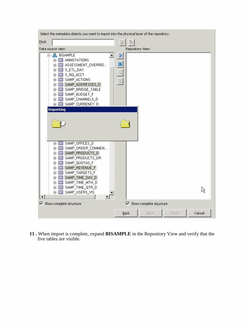
11 . When import is complete, expand BISAMPLE in the Repository View and verify that the
five tables are visible.

12 . Click Finish to open the repository.

13 . Expand orcl > BISAMPLE and confirm that the five tables are imported into the Physical
layer of the repository. Verify Connection
1 . Select Tools > Update All Row Counts.

2 . When update row counts completes, move the cursor over the tables and observe that row count
information is now visible, including when the row count was last updated.
3 . Expand tables and observe that row count information is also visible for individual columns.

4 . Right-click a table and select View Data to view the data for the table.

5 . Close the View Data dialog box when you are done. It is a good idea to update row counts or
view data after an import to verify connectivity. Viewing data or updating row count, if successful, tells you that your connection is configured correctly.

Create Aliases 1 . It is recommended that you use table aliases frequently in the Physical layer to eliminate
extraneous joins and to include best practice naming conventions for physical table names. Right-click SAMP_TIME_DAY_D and select New Object > Alias to open the Physical Table dialog box.
2 . Enter D1 Time in the Name field.

3 . In the Description field, enter Time Dimension Alias at day grain. Stores one record for each day.

4 . Click the Columns tab. Note that alias tables inherit all column definitions from the source table.

5 . Click OK to close the Physical Table dialog box.
6 . Repeat the steps and create the following aliases for the remaining physical tables.
SAMP_ADDRESSES_D = D4 Address
SAMP_CUSTOMERS_D = D3 Customer
SAMP_PRODUCTS_D = D2 Product
SAMP_REVENUE_F = F1 Revenue

Create Keys and Joins
1 . Select the five alias tables in the Physical layer. 2 . Right-click one of the highlighted alias tables and select Physical Diagram > Selected
Object(s) Only to open the Physical Diagram. Alternatively, you can click the Physical Diagram button on the toolbar.

3 . Rearrange the alias table objects so they are all visible.

4 . You may want to adjust the objects in the Physical Diagram. If so, use the toolbar buttons to
zoom in, zoom out, fit the diagram, collapse or expand objects, select objects, and so forth:
5 . Click the New Join button on the toolbar.
6 . Click the F1 Revenue table and then the D1 Time table. The Physical Foreign Key dialog box
opens. It matters which table you click first. The join creates a one-to-many (1:N) relationship that joins the key column in the first table to a foreign key column in the second table.
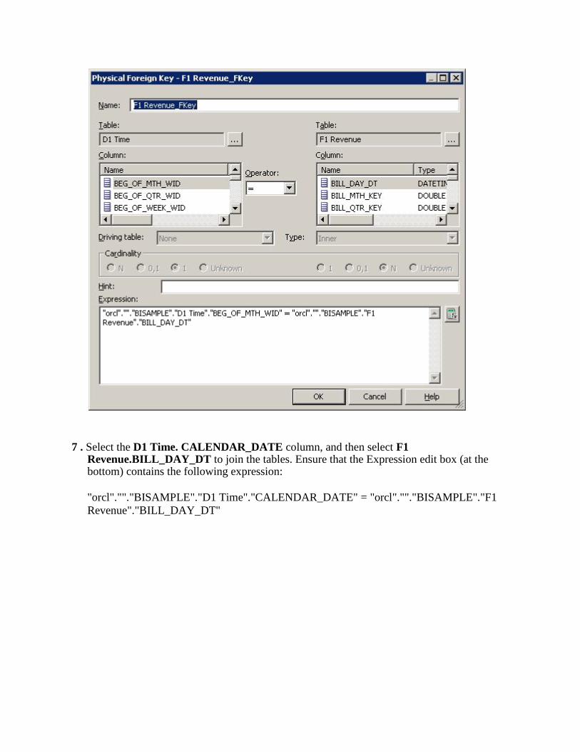
7 . Select the D1 Time. CALENDAR_DATE column, and then select F1 Revenue.BILL_DAY_DT to join the tables. Ensure that the Expression edit box (at the bottom) contains the following expression:
"orcl".""."BISAMPLE"."D1 Time"."CALENDAR_DATE" = "orcl".""."BISAMPLE"."F1
Revenue"."BILL_DAY_DT"

8 . Click OK to close the Physical Foreign Key dialog box. The join is visible in the Physical Diagram.

Please be aware of the following upgrade considerations for Oracle BI EE 11g Release 1 (11.1.1.5): Joins in the Physical and Business Model diagrams are now represented by a line
with an arrow at the "one" end of the join, rather than the line with crow�s feet at the "many" end of the join that was used in previous releases. When creating joins in the Physical and Business Model Diagrams, you now select the "many" end of the join first, and then select the "one" end of the join. In previous releases, joins in the diagrams were created by selecting the "one" end of the join first.
9 . Repeat the steps to create joins for the remaining tables. Use the following expressions as a guide. Please notice that D4 Address joins to D3 Customer.
"orcl".""."BISAMPLE"."D2 Product"."PROD_KEY" = "orcl".""."BISAMPLE"."F1
Revenue"."PROD_KEY"
"orcl".""."BISAMPLE"."D3 Customer"."CUST_KEY" = "orcl".""."BISAMPLE"."F1 Revenue"."CUST_KEY"
"orcl".""."BISAMPLE"."D4 Address"."ADDRESS_KEY" = "orcl".""."BISAMPLE"."D3

Customer"."ADDRESS_KEY"
10 . Click the Auto Layout button on the toolbar.
11 . Your diagram should look similar to the screenshot:. 12 . Click the X in the upper right corner to close the Physical Diagram.
13 . Select File > Save or click the Save button on the toolbar to save the repository.

14 . Click No when prompted to check global consistency. Checking Global Consistency checks for errors in the entire repository. Some of the more common checks are done in the Business Model and Mapping layer and Presentation layer. Since these layers are not defined yet, bypass this check until the other layers in the repository are built. You learn more about consistency check later in this tutorial.
15 . Leave the Administration Tool and the repository open for the next topic.
Congratulations! You have successfully created a new repository, imported a table schema from an external data source into the Physical layer, created aliases, and defined keys and joins.
In the next topic you learn how to build the Business Model and Mapping layer of a repository.

Building the Business Model and Mapping Layer of a Repository
In this topic you use the Oracle BI Administration Tool to build the Business Model and Mapping layer of a repository.
The Business Model and Mapping layer of the Administration Tool defines the business, or logical, model of the data and specifies the mappings between the business model and the Physical layer schemas. This layer is where the physical schemas are simplified to form the basis for the users’ view of the data. The Business Model and Mapping layer of the Administration Tool can contain one or more business model objects. A business model object contains the business model definitions and the mappings from logical to physical tables for the business model.
The main purpose of the business model is to capture how users think about their business using their own vocabulary. The business model simplifies the physical schema and maps the users’ business vocabulary to physical sources. Most of the vocabulary translates into logical columns in the business model. Collections of logical columns form logical tables. Each logical column (and hence each logical table) can have one or more physical objects as sources.
There are two main categories of logical tables: fact and dimension. Logical fact tables contain the measures by which an organization gauges its business operations and performance. Logical dimension tables contain the data used to qualify the facts.
To build the Business Model and Mapping layer of a repository, you perform the following steps:
Create a Business Model
Examine Logical Joins
Examine Logical Columns
Examine Logical Table Sources
Rename Logical Objects Manually
Rename Logical Objects Using the Rename Wizard
Delete Unnecessary Logical Objects
Create Simple Measures
Create a Business Model
1. Right-click the white space in the Business Model and Mapping layer and select New Business

Model to open the Business Model dialog box.
2. Enter Sample Sales in the Name field. Leave Disabled checked.

3. Click OK. The Sample Sales business model is added to the Business Model and Mapping layer.

4. In the Physical layer, select the following four alias tables:
D1 Time
D2 Product
D3 Customer
F1 Revenue
Do not select D4 Address at this time.
5 . Drag the four alias table from the Physical layer to the Sample Sales business model in the Business Model and Mapping layer. The tables are added to the Sample Sales business model. Notice that the three dimension tables have the same icon, whereas the F1 Revenue table has an icon with a # sign, indicating it is a fact table.

Examine Logical Joins 1. Right-click the Sample Sales business model and select Business Model Diagram >
Whole Diagram to open the Business Model Diagram.
2 . If necessary, rearrange the objects so that the join relationships are visible.
Because you dragged all tables simultaneously from the Physical layer onto the business model,

the logical keys and joins are created automatically in the business model. This is because the keys and join relationships were already created in the Physical layer. However, you typically do not drag all physical tables simultaneously, except in very simple models. Later in this tutorial, you learn how to manually build logical keys and joins in the Business Model and Mapping layer. The process is very similar to building joins in the Physical layer.
3. Double-click any one of the joins in the diagram to open the Logical Join dialog box. In this
example the join between D1 Time and F1 Revenue is selected. Notice that there is no join expression. Joins in the BMM layer are logical joins. Logical joins express the cardinality relationships between logical tables and are a requirement for a valid business model. Specifying the logical table joins is required so that Oracle BI Server has necessary metadata to translate logical requests against the business model into SQL queries against the physical data sources. Logical joins help Oracle BI Server understand the relationships between the various pieces of the business model. When a query is sent to Oracle BI Server, the server determines how to construct physical queries by examining how the logical model is structured. Examining logical joins is an integral part of this process. The Administration Tool considers a table to be a logical fact table if it is at the “many” end of all

logical joins that connect it to other logical tables.
4 . Click OK to close the Logical Join dialog box.
5 . Click the X to close the Business Model Diagram.
Examine Logical Columns 1 . Expand the D1 Time logical table. Notice that logical columns were created automatically for
each table when you dragged the alias tables from the Physical layer to the BMM layer.
Examine Logical Table Sources
1 . Expand the Sources folder for the D1 Time logical table. Notice there is a logical table source, D1 Time. This logical table source maps to the D1 Time alias table in the Physical layer.

2 . Double-click the D1 Time logical table source (not the logical table) to open the Logical Table Source dialog box.

3 . On the General tab, rename the D1 Time logical table source to LTS1 Time. Notice that the logical table to physical table mapping is defined in the "Map to these tables" section.

4 . On the Column Mapping tab, notice that logical column to physical column mappings are defined. If mappings are not visible, select Show mapped columns.

5 . You learn more about the Content and Parent-Child Settings tabs later in this tutorial when you build logical dimension hierarchies. Click OK to close the Logical Table Source dialog box. If desired, explore logical table sources for the remaining logical tables.

Rename Logical Objects Manually 1. Expand the D1 Time logical table.

2. Click on the first logical column, BEG_OF_MONTH_WID, to highlight it. 3. Click on BEG_OF_MONTH_WID again to make it editable.

4 . Rename BEG_OF_MONTH_WID to Beg of Mth Wid. This is the manual method for renaming objects. You can also right-click an object and select Rename to manually rename an object.
Rename Objects Using the Rename Wizard 1 . Select Tools > Utilities > Rename Wizard > Execute to open the Rename Wizard. 2 . In the Select Objects screen, click Business Model and Mapping in the middle pane.

3 . Expand the Sample Sales business model.

4 . Expand the D1 Time logical table.
5 . Use Shift+click to select all of the logical columns except for the column you already renamed, Beg of Mth Wid.

6 . Click Add to add the columns to the right pane.

7 . Repeat the steps for the three remaining logical tables so that all logical columns from the
Sample Sales business model are added to the right pane. Only the columns from F1 Revenue are shown in the screenshot.

8 . Click Next to move to the Select Types screen.

Notice that Logical Column is selected. If you had selected other object types, such as logical tables, the type would have appeared here.
9 . Click Next to open the Select Rules screen.

10 . In the Select Rules screen, select All text lowercase and click Add to add the rule to the lower pane.

11 . Add the rule Change each occurrence of '_' into a space.

12 . Add the rule First letter of each word capital. 13 . Click Next to open the Finish screen. Verify that all logical columns will be named according
to the rename rules you selected.

14 . Click Finish. 15 . In the Business Model and Mapping layer, expand the logical tables and confirm that all logical
columns have been renamed as expected. The screenshot shows only the columns in D1 Time.

16 . In the Physical layer, expand the alias tables and confirm that all physical columns have not been renamed. The point here is you can change object names in the BMM layer without impacting object names in the Physical layer. When logical objects are renamed, the relationships between logical objects and physical objects are maintained by the logical column to physical column mappings.
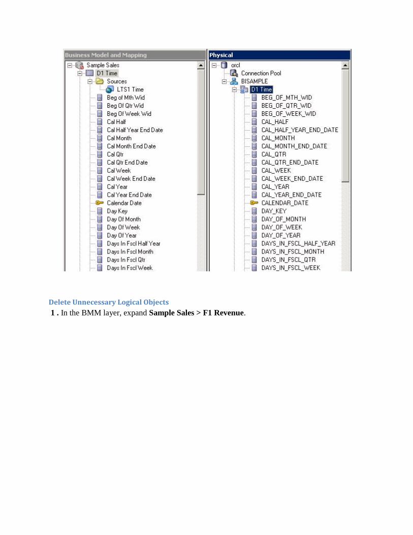
Delete Unnecessary Logical Objects 1 . In the BMM layer, expand Sample Sales > F1 Revenue.

2 . Use Ctrl+Click to select all F1 Revenue logical columns except for Revenue and Units.

3 . Right-click any one of the highlighted logical columns and select Delete. Alternatively you can select Edit > Delete or press the Delete key on your keyboard.

4 . Click Yes to confirm the delete. 5 . Confirm that F1 Revenue contains only the Revenue and Units columns.

Create Simple Measures 1 . Double-click the Revenue logical column to open the Logical Column dialog box. 2 . Click the Aggregation tab.

3 . Change the default aggregation rule to Sum.
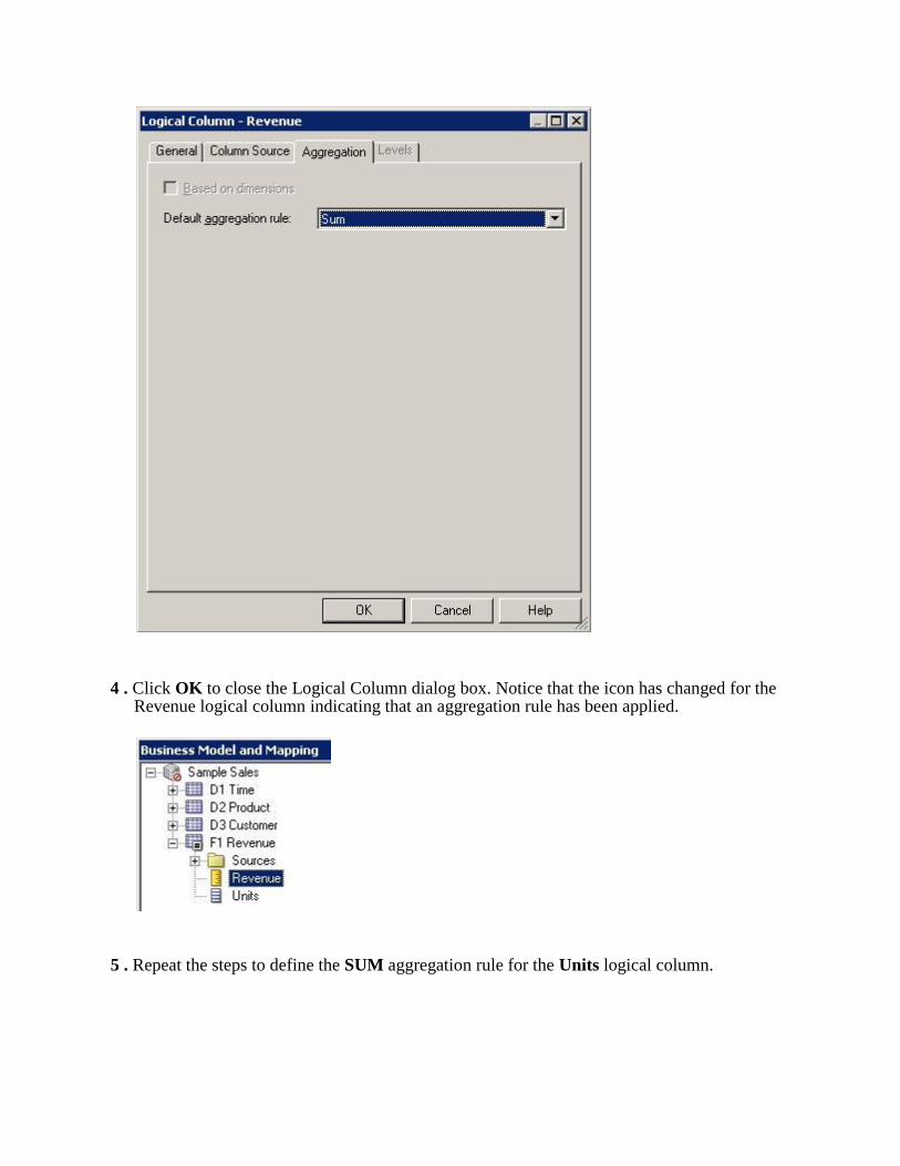
4 . Click OK to close the Logical Column dialog box. Notice that the icon has changed for the Revenue logical column indicating that an aggregation rule has been applied.
5 . Repeat the steps to define the SUM aggregation rule for the Units logical column.
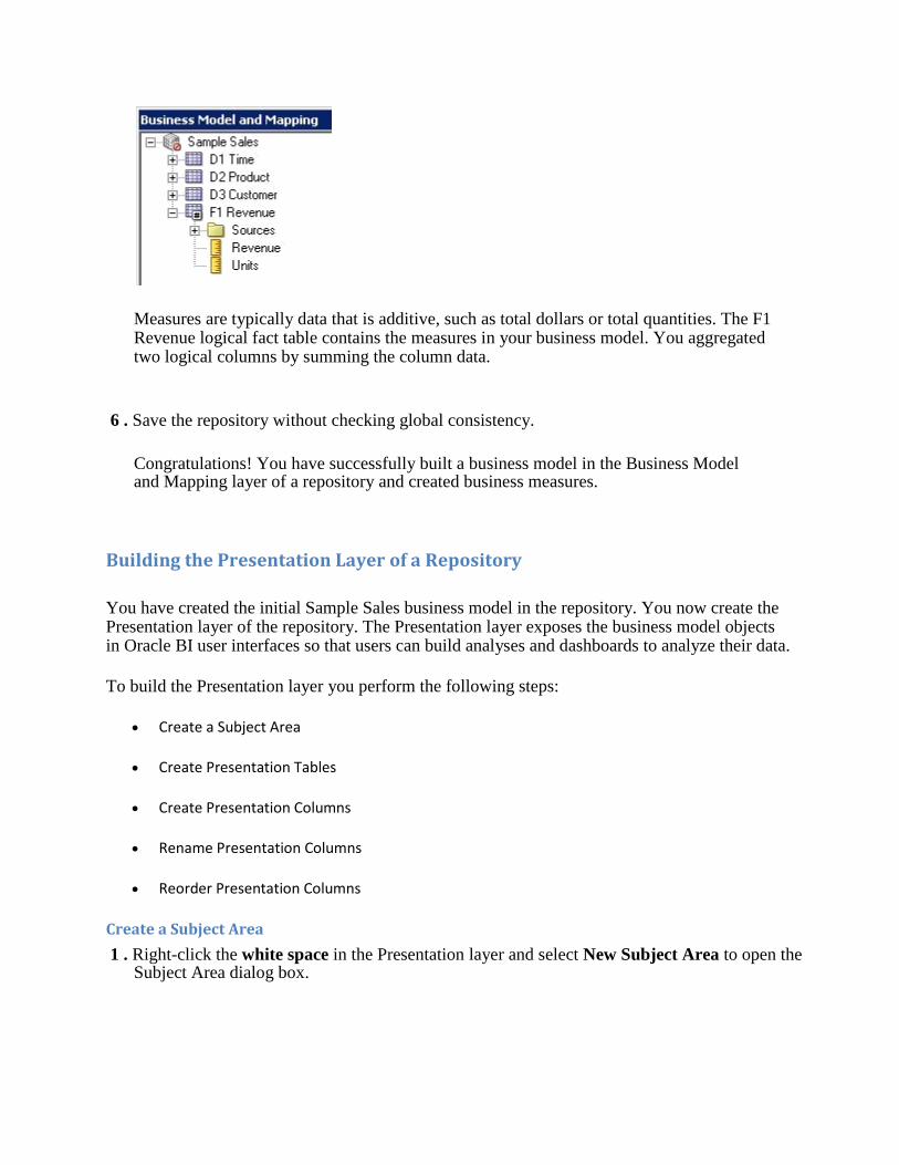
Measures are typically data that is additive, such as total dollars or total quantities. The F1 Revenue logical fact table contains the measures in your business model. You aggregated two logical columns by summing the column data.
6 . Save the repository without checking global consistency.
Congratulations! You have successfully built a business model in the Business Model and Mapping layer of a repository and created business measures.
Building the Presentation Layer of a Repository
You have created the initial Sample Sales business model in the repository. You now create the Presentation layer of the repository. The Presentation layer exposes the business model objects in Oracle BI user interfaces so that users can build analyses and dashboards to analyze their data.
To build the Presentation layer you perform the following steps:
Create a Subject Area
Create Presentation Tables
Create Presentation Columns
Rename Presentation Columns
Reorder Presentation Columns
Create a Subject Area 1 . Right-click the white space in the Presentation layer and select New Subject Area to open the
Subject Area dialog box.

2 . On the General tab, enter Sample Sales as the name of the subject area.

3 . Click OK to close the Subject Area dialog box. The Sample Sales subject area is added to the
Presentation layer.
Create Presentation Tables 1. Right-click the Sample Sales subject area and select New Presentation Table to open
the Presentation Table dialog box.
2. On the General tab, enter Time as the name of the presentation table.

3 . Click OK to close the Presentation Table dialog box. The Time presentation table is added to the
Sample Sales subject area.
4 . Repeat the process and add three more presentation tables: Products, Customers, and Base Facts.
Please note that you are using the manual method for creating Presentation layer objects. For simple models it is also possible to drag objects from the BMM layer to the Presentation layer to

create the Presentation layer objects. When you create presentation objects by dragging from the BMM layer, the business model becomes a subject area, the logical tables become presentation tables, and the logical columns become presentation columns. Note that all objects within a subject area must derive from a single business model.
Create Presentation Columns
1. In the BMM layer, expand the D1 Time logical table.
2. Use Ctrl+ Click to select the following logical columns:
Calendar Date
Per Name Half
Per Name Month
Per Name Qtr
Per Name Week
Per Name Year.

3 . Drag the selected logical columns to the Time presentation table in the Presentation layer.

4 . Repeat the process and add the following logical columns to the remaining presentation tables:
Products: Drag Brand, Lob, Prod Dsc, Type from D2 Product.
Customers: Drag Cust Key, Name from D3 Customer.
Base Facts: Drag Revenue, Units from F1 Revenue.
Rename Presentation Columns 1. In the Presentation layer, expand the Products presentation table.

2. Double-click the Lob presentation column to open the Presentation Column dialog box. On
the General tab notice that "Use Logical Column Name" is selected. When you drag a logical column to a presentation table, the resulting presentation column inherits the logical column name by default. In this example the Lob presentation column inherits the name of the logical column "Sample Sales"."D2 Product"."Lob".
3 . Deselect Use Logical Column Name. The Name field is now editable.

4 . Enter Line of Business in the Name field.
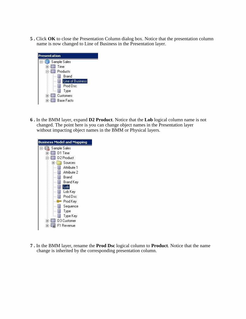
5 . Click OK to close the Presentation Column dialog box. Notice that the presentation column
name is now changed to Line of Business in the Presentation layer.
6 . In the BMM layer, expand D2 Product. Notice that the Lob logical column name is not
changed. The point here is you can change object names in the Presentation layer without impacting object names in the BMM or Physical layers.
7 . In the BMM layer, rename the Prod Dsc logical column to Product. Notice that the name change is inherited by the corresponding presentation column.

8 . Make the following name changes to logical objects in the BMM layer so that the names of the
corresponding presentation columns are also changed:
For the D3 Customer logical table:
Change Cust Key to Customer Number.
Change Name to Customer Name.

9 . Confirm that the corresponding presentation column names are changed. Reorder Presentation Columns 1. In the Presentation layer, double-click the Time presentation table to open the Presentation Table
dialog box.
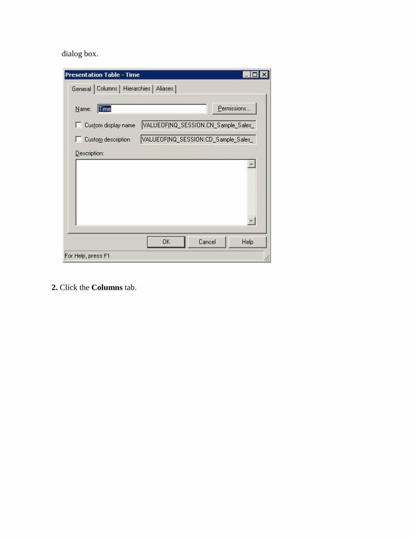
2. Click the Columns tab.

3 . Select columns and use the up and down arrows, or drag the columns. to rearrange the
presentation columns into the following order from top to bottom:
Per Name Year
Per Name Half
Per Name Qtr
Per Name Month
Per Name Week
Calendar Date

4 . Click OK to close the Presentation Table dialog box and confirm that the presentation column
order is changed in the Presentation layer.
5 . Repeat the steps to reorder the columns in the Products presentation table:
Brand
Line of Business
Type
Product

6 . Save the repository without checking global consistency.
Congratulations! You have successfully built the Presentation layer of a repository.
Testing and Validating a Repository
You have finished building an initial business model and now need to test and validate the repository before continuing. You begin by checking the repository for errors using the consistency checking option. Next you load the repository into Oracle BI Server memory. You then test the repository by running an Oracle BI analysis and verifying the results. Finally, you examine the query log file to observe the SQL generated by Oracle BI Server.
To test and validate a repository you perform the following steps:
Check Consistency
Disable Caching
Load the Repository
Set Up Query Logging
Create and Run and Analysis
Check the Query Log
Check Consistency 1. Select File > Check Global Consistency.

2. You should receive the message Business model "Sample Sales" is consistent. Do you
want to mark it as available for queries?
3 . Click Yes. You should receive the message: Consistency check didn't find any errors,
warnings or best practice violations.

If you do not receive this message, you must fix any consistency check errors or warnings before proceeding.
4 . Click OK. Notice that the Sample Sales business model icon in the BMM layer is now green,
indicating it is available for queries.
5 . Save the repository without checking global consistency again.
6 . Select File > Close to close the repository. Leave the Administration Tool open.
Disable Caching 1. Open a browser and enter the following URL to navigate to Enterprise Manager
Fusion Middleware Control:
http://<machine name>:7001/em
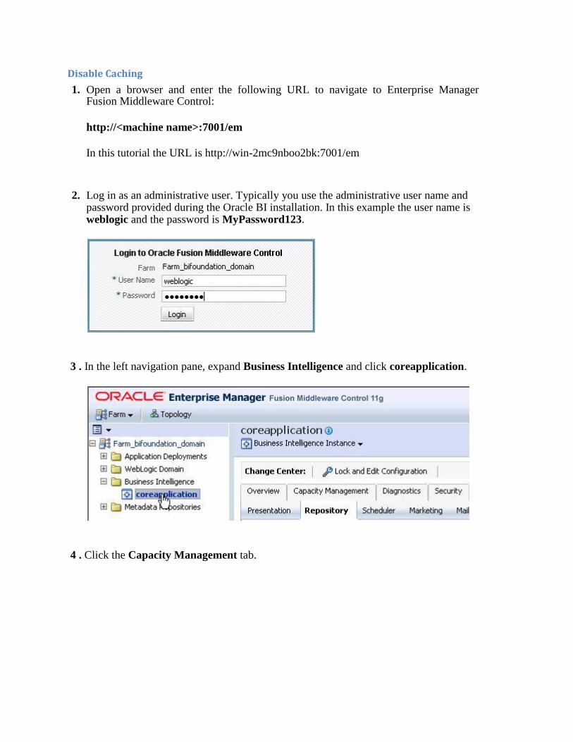
In this tutorial the URL is http://win-2mc9nboo2bk:7001/em 2. Log in as an administrative user. Typically you use the administrative user name and
password provided during the Oracle BI installation. In this example the user name is weblogic and the password is MyPassword123.
3 . In the left navigation pane, expand Business Intelligence and click coreapplication.
4 . Click the Capacity Management tab.

5 . Click the Performance sub tab.
6 . Locate the Enable BI Server Cache section. Cache is enabled by default. 7 . Click Lock and Edit Configuration.

8 . Click Close when you receive the confirmation message "Lock and Edit Configuration -
Completed Successfully."
9 . Deselect Cache enabled. Caching is typically not used during development. Disabling cache
improves query performance.
10 . Click Apply.

11 . Click Activate Changes.
12 . Click Close when you receive the confirmation message Activate Changes -
Completed Successfully.

13 . Do not click Restart to apply recent changes yet. You do that after uploading the repository
in the next set of steps. Load the Repository 1. Click the Deployment tab.
2 . Click the Repository sub tab.

3 . Click Lock and Edit Configuration. 4 . Click Close when you receive the confirmation message "Lock and Edit Configuration -
Completed Successfully."
5 . In the "Upload BI Server Repository" section, click Browse to open the Choose file dialog box.
6 . By default, the Choose file dialog box should open to the repository directory. If not, navigate
to the repository directory with the BISAMPLE repository.

7 . Select the BISAMPLE.rpd file and click Open.

8 . Enter admin123 as the repository password and confirm the password.
9 . Click Apply.

10 . In the BI Server Repository section, confirm that the Default RPD is now BISAMPLE with
an extension. In this example the file name is BISAMPLE_BI0025.

11 . Click Activate Changes.

12 . Click Close when you receive the confirmation message Activate Changes -
Completed Successfully.
13 . Click Restart to apply recent changes to navigate to the Overview page.

14 . On the Overview page, click Restart. 15 . Click Yes when you receive the message Are you sure you want to restart all BI

components?
16 . Allow the Restart All processing to complete. This may take a few moments.
17 . Click Close when you receive the confirmation message Restart All - Completed Successfully.
18 . Confirm that System Components are 100% and that five components are up. Leave
Fusion Middleware Control open.

Set Up Query Logging 1 . Return to the Administration Tool, which should still be open. 2 . Select File > Open > Online to open the repository in online mode. You use online mode to
view and modify a repository while it is loaded into the Oracle BI Server. The Oracle BI Server must be running to open a repository in online mode.
3 . Enter admin123 as the repository password and enter your administrative user name and
password. (weblogic / MyPassword123)

4 . Click Open to open the repository in online mode. 5 . Select Manage > Identity to open Identity Manager.

6 . In the left pane, select BI Repository.
7 . Select Action > Set Online User Filter.

8 . Enter an asterisk and click OK to fetch users from the identity store.

9 . In the right pane, double-click your administrative user to open the User dialog box. In this
example the administrative user is weblogic. 10 . In the User dialog box, on the User tab, set Logging level to 2. 11 . Click OK to open the Check Out Objects dialog box.

12 . In the Check Out Objects dialog box, click Check Out. When you are working in a
repository open in online mode, you are prompted to check out objects when you attempt to perform various operations.
13 . Select Action > Close to close Identity Manager. 14 . Select File > Check In Changes. Alternatively, you can click the Check In Changes icon
on the toolbar.

15 . Save the repository. There is no need to check consistency. 16 . Select File > Copy As to save a copy of the online repository with the security changes.

17 . In the Save Copy As dialog box, save the file as BISAMPLE.rpd, replacing the existing BISAMPLE repository.
18 . Click Yes when asked if you want to replace the existing BISAMPLE repository. This will create a new BISAMPLE repository with query logging set for the weblogic user.

19 . Select File > Close to close the repository.
20 . Click OK when you receive the following message:
"In order for your online changes to take effect, you will have to manually restart each non-master Oracle BI Server instance in the cluster."

21 . Leave the Administration Tool open.
Create and Run an Analysis 1. Open a browser or a new browser tab and enter the following URL to navigate to
Oracle Business Intelligence:
http://<machine name>:7001/analytics
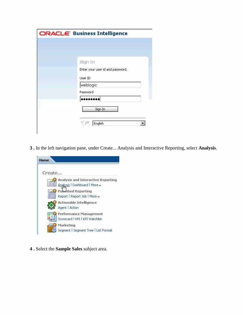
In this tutorial the URL is http://win-2mc9nboo2bk:7001/analytics 2. Sign in as an administrative user. Typically you use the administrative user name and
password provided during the Oracle BI installation. In this example the user name is weblogic and the password is MyPassword123. If you need help identifying a user name and password, contact your company's Oracle BI Administrator.

3 . In the left navigation pane, under Create... Analysis and Interactive Reporting, select Analysis. 4 . Select the Sample Sales subject area.
5 . In the left navigation pane, expand the folders in the Sample Sales subject area and confirm that
the user interface matches the presentation layer of the repository.

6 . Double-click the following column names in the Subject Areas pane to add them to the analysis:
Time.Per Name Year
Products.Type
Base Facts.Revenue
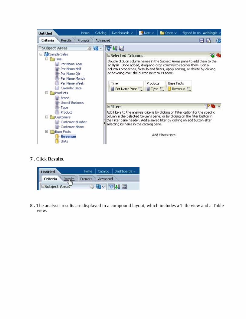
7 . Click Results. 8 . The analysis results are displayed in a compound layout, which includes a Title view and a Table
view.

9 . Use the buttons at the bottom of the compound layout to view additional rows.

Check the Query Log 1 . Return to Fusion Middleware Control, which should still be open. If not, enter
http://win-2mc9nboo2bk:7001/em in a browser and sign in as your administrative user.
2 . Click the Diagnostics tab.

3 . Click the Log Messages sub tab.
4 . Scroll to the bottom of the window to the View / Search Log Files section.
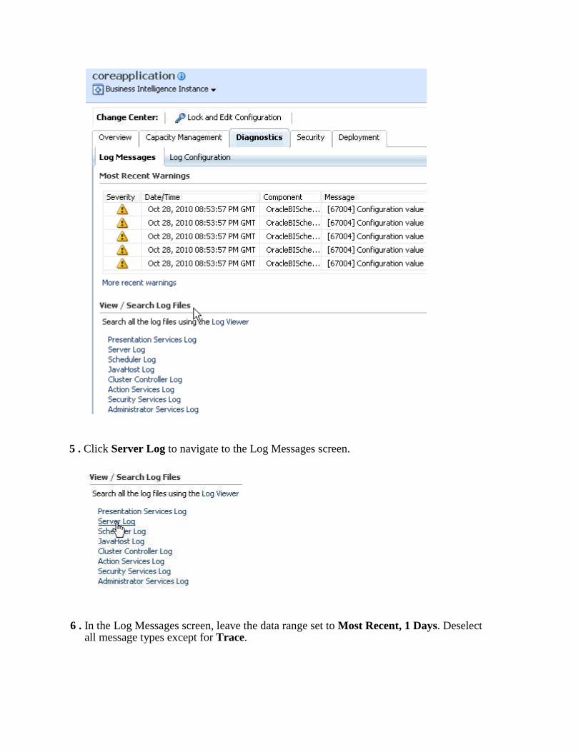
5 . Click Server Log to navigate to the Log Messages screen. 6 . In the Log Messages screen, leave the data range set to Most Recent, 1 Days. Deselect
all message types except for Trace.

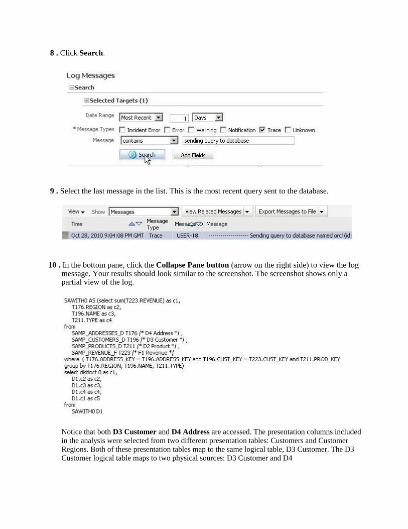
7 . In the Message field, enter sending query to database.
8 . Click Search.
9 . There should be only one message at this point, but if there are more than one, select the
last message in the list. This is the most recent query sent to the database.
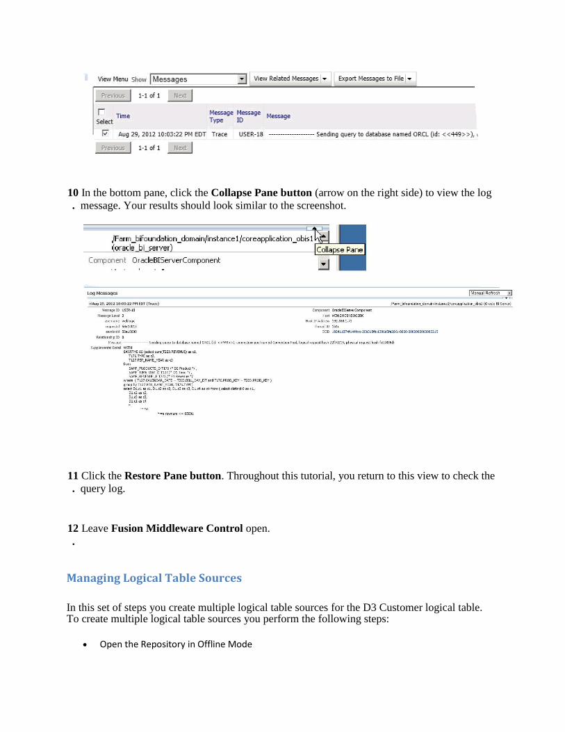
10 In the bottom pane, click the Collapse Pane button (arrow on the right side) to view the log
. message. Your results should look similar to the screenshot.
11 Click the Restore Pane button. Throughout this tutorial, you return to this view to check the
. query log.
12 Leave Fusion Middleware Control open. .
Managing Logical Table Sources
In this set of steps you create multiple logical table sources for the D3 Customer logical table. To create multiple logical table sources you perform the following steps:
Open the Repository in Offline Mode

Add a New Logical Table Source
Create Presentation Layer Objects
Load the Repository
Create and Run an Analysis
Check the Query Log
Open the Repository in Offline Mode 1 . Return to the Administration Tool, which should still be open. If not, select Start > Programs >
Oracle Business Intelligence > BI Administration. 2 . Open the BISAMPLE repository in offline mode with repository password is admin123. Recall
that earlier in this tutorial you created a copy of the online repository and saved it as BISAMPLE.rpd.
3 . Select Manage > Identity to open Identity Manager.
4 . Select BI Repository in the left pane.

5 . Recall that earlier in this tutorial you created a copy of the online repository with logging level defined for the administrative user. Confirm that your administrative user is visible in the right pane. In this example the administrative user is weblogic.

6 . Double-click the administrative user to open the User dialog box. On the User tab, confirm that
logging level is set to 2. 7 . Click Cancel to close the User dialog box. 8 . Select Action > Close to close Identity Manager. The offline BISAMPLE repository now has a
user with a logging level set to 2. This will allow you to check the query log as you complete the remaining exercises in this tutorial. You will not have to repeat the steps of copying an online repository.
Add a New Logical Table Source
1 . In the BMM layer, expand Sample Sales > D3 Customer > Sources. Notice that the D3 Customer logical table has one logical table source named D3 Customer.

2 . Rename the D3 Customer logical table source (not the logical table) to LTS1 Customer.

3 . Double-click LTS1 Customer to open the Logical Table Source dialog box. 4 . Click the Column Mapping tab and notice that all logical columns map to physical columns in
the same physical table: D3 Customer. It may be necessary to scroll to the right to see the Physical Table column. Make sure "Show mapped columns" is selected.

5 . Click OK to close the Logical Table Source dialog box.
6 . In the Physical layer, expand orcl > BISAMPLE.

7 . Drag D4 Address from the Physical layer to the D3 Customer logical table in the BMM layer.
Notice this creates a new logical table source named D4 Address for the D3 Customer logical table. It also creates new logical columns that map to the D4 Address physical table.

8 . In the BMM layer, double-click the new D4 Address logical table source to open the Logical Table Source dialog box.

9 . On the General tab, enter LTS2 Customer Address in the Name field.

10 . Click the Column Mapping tab and notice that all logical columns map to physical columns in the same physical table: D4 Address. If necessary, select Show mapped columns and deselect Show unmapped columns.

11 . Click OK to close the Logical Table Source dialog box.

12 . Confirm that the D3 Customer logical table now has two logical table sources: LTS1 Customer and LTS2 Customer Address. A single logical table now maps to two physical sources.

13 . Right-click the new ADDRESS_KEY column and select Delete. This is a duplicate column
and is not needed. 14 . Click Yes to confirm the delete.
15 . Use the Rename Wizard or a manual renaming technique to rename the new address logical
columns (with uppercase letters) in D3 Customer. Your results should look similar to the screenshot. Hint: To use the Rename Wizard, select all of the new logical columns, then right-

click any one of the highlighted columns and select Rename Wizard to launch the wizard.
16 . Rename the remaining logical table sources according to the following table. Recall that logical table sources are located in the Sources folder for a logical table. For example: D2 Product > Sources.
Logical Table Source Rename
D2 Product LTS1 Product

F1 Revenue LTS1 Revenue
Your results should look similar to the screenshot.
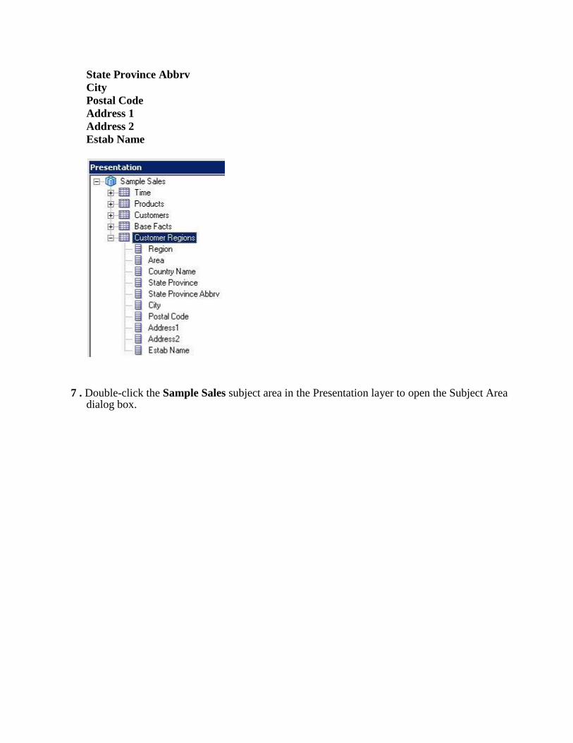
Create Presentation Layer Objects 1 . In the Presentation layer, right-click the Sample Sales subject area and select New Presentation
Table to open the Presentation Table dialog box.

2 . On the General tab, enter Customer Regions in the Name field.

3 . Click OK to close the Presentation Table dialog box. Confirm that the Customer Regions
presentation table is added to the Sample Sales subject area in the Presentation layer. 4 . In the BMM layer, expand Sample Sales > D3 Customer.

5 . Drag the following logical columns from D3 Customer to Customer Regions in the Presentation layer:
Address 1
Address 2
Area
City
Country Name Estab Name
Postal Code Region

State Province
State Province Abbrv
Your column names may be slightly different depending on how you renamed them.
6 . Reorder the Customer Regions presentation columns in the following order, from top to bottom:
Region
Area
Country Name State Province
State Province Abbrv
City
Postal Code
Address 1
Address 2
Estab Name
7 . Double-click the Sample Sales subject area in the Presentation layer to open the Subject Area
dialog box.

8 . Click the Presentation Tables tab.

9 . Reorder the presentation tables so that Customer Regions appears after Customers. 10 . Click OK to close the Subject Area dialog box. Confirm that the presentation tables appear
in the expected order.
You now have two presentation tables, Customers and Customer Regions, mapped to the same logical table, D3 Customer. The D3 Customer logical table is mapped to two physical sources: D3 Customer and D4 Address.
11 . Save the repository and check global consistency when prompted. You should receive a
message that there are no errors, warnings, or best practice violations to report.

If you do receive any consistency check errors or warnings, fix them before proceeding.
12 . Click OK to close the consistency check message.
13 . Close the repository. Leave the Administration Tool open.
Load the Repository 1. Return to Fusion Middleware Control, which should still be open. If not, open a browser
and enter the following URL to navigate to Fusion Middleware Control:
http://<machine name>/:7001/em
In this tutorial the URL is http://win-2mc9nboo2bk:7001/em 2. If your session has timed out, you will need to log in again. Log in as an administrative user.
Typically you use the administrative user name and password provided during the Oracle BI installation. In this example the user name is weblogic and the password is MyPassword123.
3 . In the left navigation pane, expand Business Intelligence and click coreapplication.

4 . Click the Deployment tab. 5 . Click the Repository sub tab.
6 . Click Lock and Edit Configuration.

7 . Click Close when you receive the confirmation message Lock and Edit Configuration -
Completed Successfully.
8 . Click Browse and navigate to the directory with the BISAMPLE repository.
9 . Select the BISAMPLE.rpd file and click Open.

10 . Enter admin123 as the repository password and confirm the password.
11 . Click Apply.

12 . Confirm that the default RPD is now BISAMPLE with an extension. In this example the
file name is BISAMPLE_BI0025.

13 . Click Activate Changes.

14 . Click Close when you receive the confirmation message Activate Changes -
Completed Successfully.
15 . Click Restart to apply recent changes to navigate to the Overview page.

16 . On the Overview page, click Restart. 17 . Click Yes when you receive the message Are you sure you want to restart all BI

components?
18 . Allow the processing to complete.
19 . Click Close when you receive the message Restart All - Completed Successfully.
Create and Run an Analysis 1. Return to Oracle BI, which should still be open. If not, open a browser or browser tab and
enter the following URL to navigate to Oracle Business Intelligence:
http://<machine name>/:7001/analytics
In this tutorial the URL is http://win-2mc9nboo2bk:7001/analytics. 2. If your previous session has timed out, sign in as an administrative user. Typically you use
the administrative user name and password provided during the Oracle BI installation. In this example the user name is weblogic and the password is MyPassword123.
3 . In the left navigation pane, under Create... Analysis and Interactive Reporting, select Analysis.
4 . Select the Sample Sales subject area.

5 . In the left navigation pane, expand the folders and confirm that the Customer Regions folder
and corresponding columns appear.
6 . Create the following analysis by double-clicking column names in the Subject Areas pane:
Customer Regions.Region Customers.Customer Name
Products.Type
Base Facts.Revenue 7 . Click Results to view the analysis results. Use the buttons at the bottom of the results screen to

see more rows.
Check the Query Log 1 . Return to Fusion Middleware Control, which should still be open.
2 . Click the Diagnostics tab.

3 . Click the Log Messages sub tab.
4 . Scroll to the bottom of the window to the View / Search Log Files section.

5 . Click Server Log to navigate to the Log Messages screen. 6 . In the Log Messages screen, leave the data range set to Most Recent, 1 Days. Deselect all
message types except for Trace. 7 . In the Message field, enter sending query to database.
8 . Click Search. 9 . Select the last message in the list. This is the most recent query sent to the database.
10 . In the bottom pane, click the Collapse Pane button (arrow on the right side) to view the log message. Your results should look similar to the screenshot. The screenshot shows only a partial view of the log. Notice that both D3 Customer and D4 Address are accessed. The presentation columns included in the analysis were selected from two different presentation tables: Customers and Customer Regions. Both of these presentation tables map to the same logical table, D3 Customer. The D3 Customer logical table maps to two physical sources: D3 Customer and D4

Address.
11 . Click the Restore Pane button.
12 . Leave Enterprise Manager open.
Creating Calculation Measures
In this set of steps you use existing measures to created a derived calculation measure. To create a derived calculation measure you perform the following steps:
Open the Repository in Offline Mode
Create a Calculation Measure Derived from Existing Columns
Create a Calculation Measure Using a Function
Load the Repository
Create and Run an Analysis
Check the Query Log
Open the Repository in Offline Mode 1 . Return to the Administration Tool, which should still be open. If not, select Start > Programs >
Oracle Business Intelligence > BI Administration.
2 . Select File > Open > Offline.

3 . Select BISAMPLE.rpd and click Open. Do not select any BISAMPLE repository with an extension, for example, BISAMPLE_BI0025.rpd. Recall that these are the repositories that have been loaded into Oracle BI Server memory.
4 . Enter admin123 as the repository password and click OK to open the repository.
Create a Calculation Measure Derived from Existing Columns 1 . In the BMM layer, expand Sample Sales > F1 Revenue.
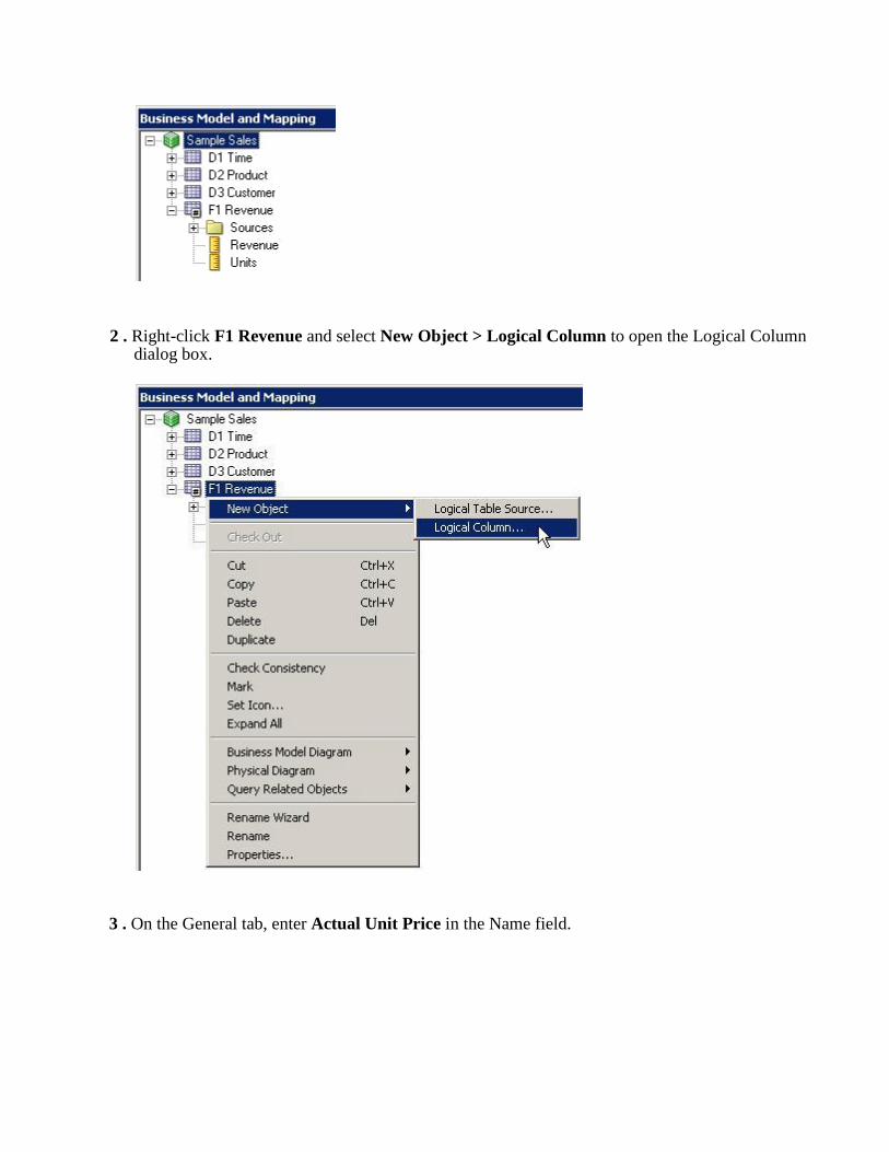
2 . Right-click F1 Revenue and select New Object > Logical Column to open the Logical Column
dialog box.
3 . On the General tab, enter Actual Unit Price in the Name field.

4 . Click the Column Source tab.

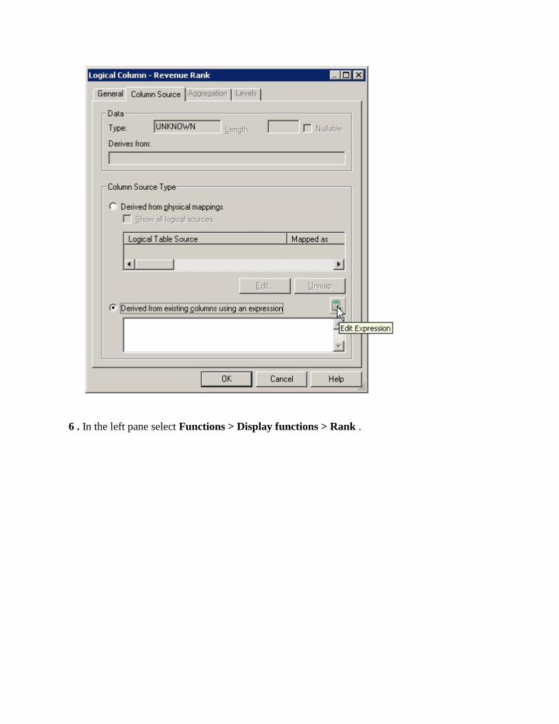
5 . Select Derived from existing columns using an expression.

6 . Click the Edit Expression button to open Expression Builder.

7 . In the left pane select Logical Tables > F1 Revenue > Revenue.

8 . Click the Insert selected item button to move the Revenue column to the right pane.

9 . Click the division operator to add it to the expression.

10 . In the left pane select Logical Tables > F1 Revenue and then double-click Units to add it to the expression.
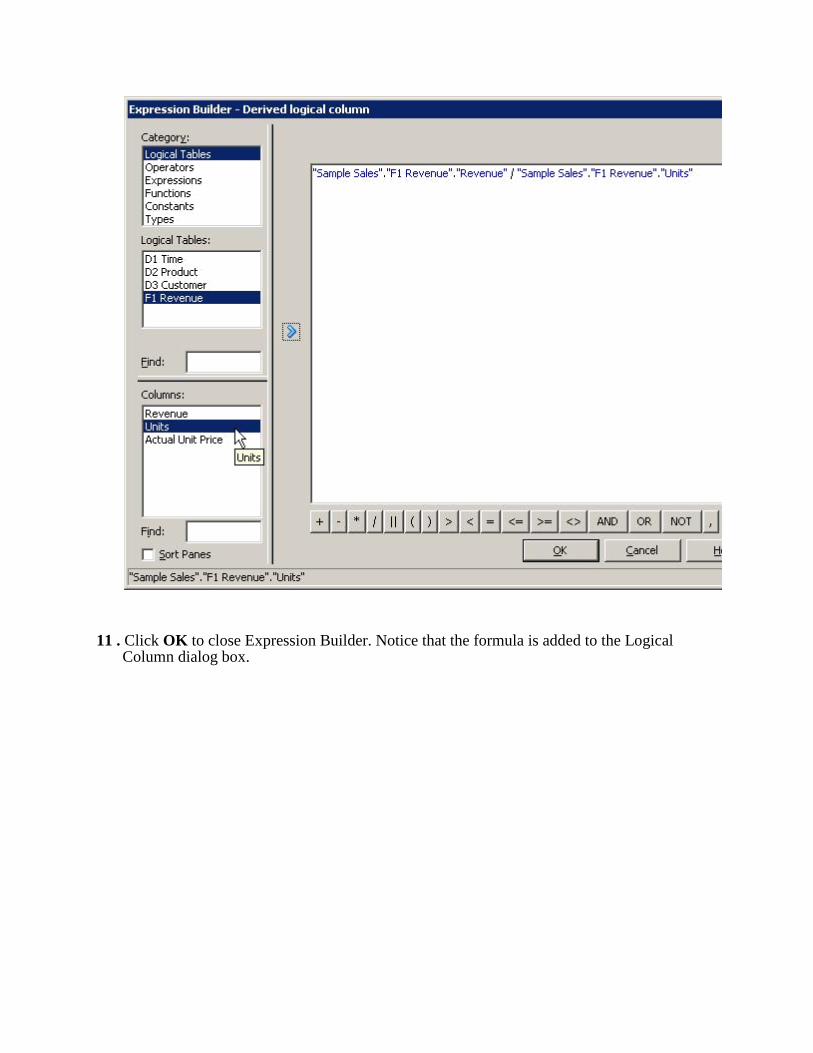
11 . Click OK to close Expression Builder. Notice that the formula is added to the Logical Column dialog box.

12 . Click OK to close the Logical Column dialog box. The Actual Unit Price calculated measure is added to the business model.
13 . Drag Actual Unit Price from the BMM layer to the Base Facts presentation table in the Presentation layer.

14 . Save the repository and check consistency. Fix any errors or warnings before proceeding.
Create a Calculation Measure Using a Function 1 . In the BMM layer, right-click F1 Revenue and select New Object > Logical Column to open
the Logical Column dialog box.

2 . On the General tab, enter Revenue Rank in the Name field. 3 . Click the Column Source tab.
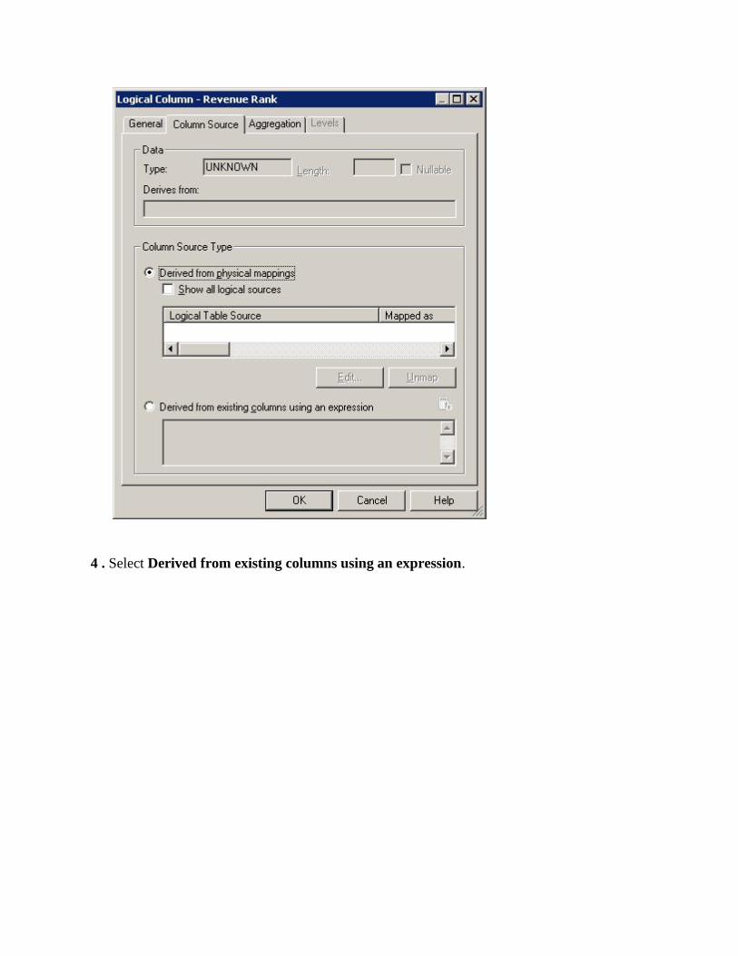
4 . Select Derived from existing columns using an expression.

5 . Click the Edit Expression button to open Expression Builder.
6 . In the left pane select Functions > Display functions > Rank .

7 . Click the Insert selected item button to move the Rank function to the right pane.
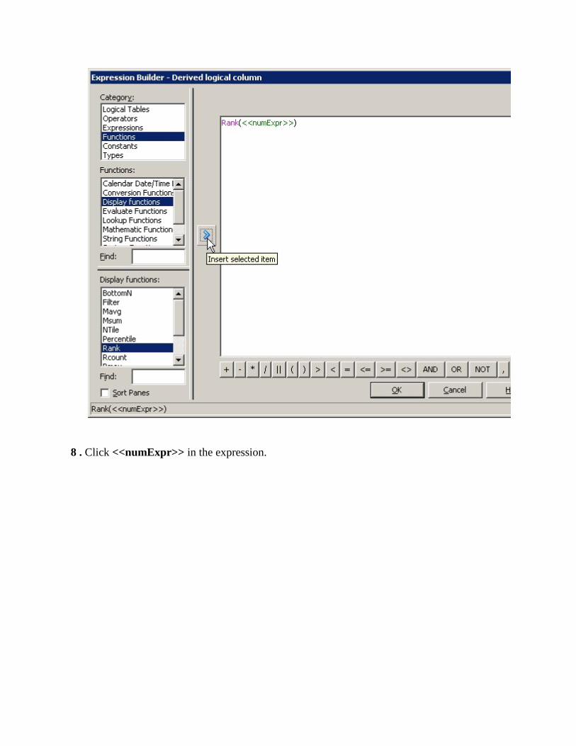
8 . Click <<numExpr>> in the expression.

9 . In the left pane select Logical Tables > F1 Revenue and then double-click Revenue to add it to the expression.

10 . Click OK to close Expression Builder. Notice that the formula is added to the Logical Column dialog box.

11 . Click OK to close the Logical Column dialog box. The Revenue Rank calculated measure is added to the business model.
12 . Drag Revenue Rank from the BMM layer to the Base Facts presentation table in
the Presentation layer.

13 . Save the repository and check consistency. Fix any errors or warnings before proceeding. 14 . Close the repository. Leave the Admin Tool open.
Load the Repository 1. Return to Fusion Middleware Control, which should still be open. If not, open a browser
and enter the following URL to navigate to Fusion Middleware Control Enterprise Manager:
http://<machine name>/:7001/em
In this tutorial the URL is http://win-2mc9nboo2bk:7001/em 2. If necessary, log in as an administrative user. Typically you use the administrative user
name and password provided during the Oracle BI installation. In this example the user name is weblogic and the password is MyPassword123.

3 . In the left navigation pane, expand Business Intelligence and click on coreapplication.
4 . Click the Deployment tab. 5 . Click the Repository sub tab.

6 . Click Lock and Edit Configuration. 7 . Click Close when you receive the confirmation message Lock and Edit Configuration -
Completed Successfully.
8 . Click Browse and navigate to the directory with the BISAMPLE repository.

9 . Select the BISAMPLE.rpd file and click Open. 10 . Enter admin123 as the repository password and confirm the password.
11 . Click Apply.

12 . Confirm that the default RPD is now BISAMPLE with an extension. In this example the
file name is BISAMPLE_BI0025.

13 . Click Activate Changes.

14 . Click Close when you receive the confirmation message Activate Changes -
Completed Successfully.
15 . Click Restart to apply recent changes to navigate to the Overview page.

16 . On the Overview page, click Restart. 17 . Click Yes when you receive the message Are you sure you want to restart all BI

components?
18 . Allow the processing to complete.
19 . Click Close when you receive the message Restart All - Completed Successfully.
Create and Run an Analysis 1. Return to Oracle BI, which should still be open. If not, open a browser or browser tab and
enter the following URL to navigate to Oracle Business Intelligence:
http://<machine name>/:7001/analytics
In this tutorial the URL is http://win-2mc9nboo2bk:7001/analytics. 2. If necessary, log in as an administrative user. Typically you use the administrative user name and
password provided during the Oracle BI installation. In this example the user name is weblogic and the password is MyPassword123.

3 . In the left navigation pane, under Create... Analysis and Interactive Reporting, select Analysis. Hint: If your session has not timed out, you can create a new analysis by selecting New > Analysis.
4 . Select the Sample Sales subject area. 5 . In the left navigation pane, expand the Base Facts folder and confirm that the Actual Unit Price
and Revenue Rank columns are visible. 6 . Create the following analysis by double-clicking column names in the Subject Areas pane:
Products.Product
Base Facts.Revenue
Base Facts.Revenue Rank
Base Facts.Units
Base Facts.Actual Unit Price 7 . Sort Revenue Rank in ascending order.

8 . Click Results to view the analysis results.
Please note that the Actual Unit Price calculation is correct, although it does not make sense from a business perspective. For example, the unit price for an LCD HD Television would not be 9 dollars. This is a result of the underlying sample data.
Check the Query Log 1 . In this set of steps you use another method to check the query log. Click the Administration
link in the upper right.

1 . Click OK when you are asked "are you sure you want to navigate away from this page?" 1 . On the Administration page, under Session Management, select Manage Sessions.
1 . In the Cursor Cache section, locate your query and select View Log.
2 . Your log entry should look similar to the screenshot.
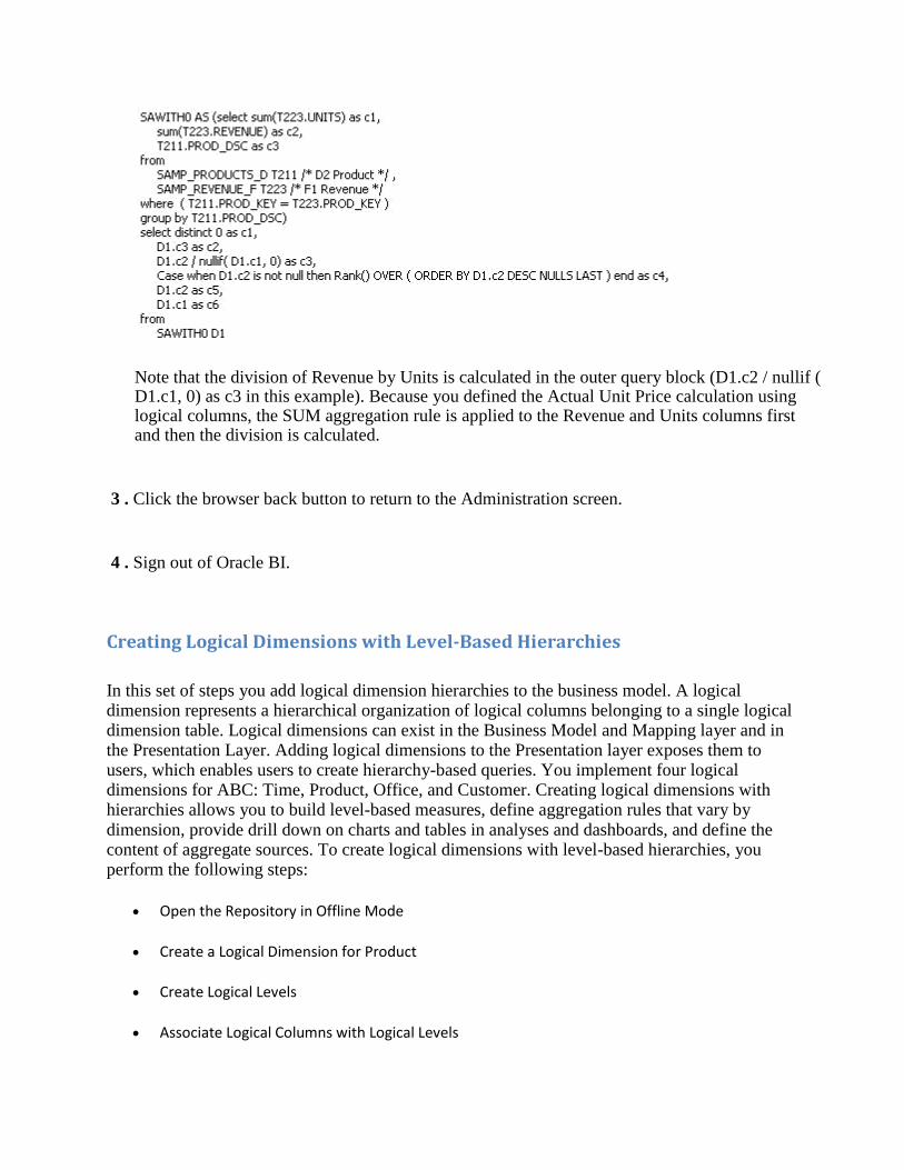
Note that the division of Revenue by Units is calculated in the outer query block (D1.c2 / nullif ( D1.c1, 0) as c3 in this example). Because you defined the Actual Unit Price calculation using logical columns, the SUM aggregation rule is applied to the Revenue and Units columns first and then the division is calculated.
3 . Click the browser back button to return to the Administration screen.
4 . Sign out of Oracle BI.
Creating Logical Dimensions with Level-Based Hierarchies
In this set of steps you add logical dimension hierarchies to the business model. A logical dimension represents a hierarchical organization of logical columns belonging to a single logical dimension table. Logical dimensions can exist in the Business Model and Mapping layer and in the Presentation Layer. Adding logical dimensions to the Presentation layer exposes them to users, which enables users to create hierarchy-based queries. You implement four logical dimensions for ABC: Time, Product, Office, and Customer. Creating logical dimensions with hierarchies allows you to build level-based measures, define aggregation rules that vary by dimension, provide drill down on charts and tables in analyses and dashboards, and define the content of aggregate sources. To create logical dimensions with level-based hierarchies, you perform the following steps:
Open the Repository in Offline Mode
Create a Logical Dimension for Product
Create Logical Levels
Associate Logical Columns with Logical Levels

Set Logical Level Keys
Create a Logical Dimension for Time
Associate Time Logical Columns with Logical Levels
Create a Logical Dimension for Customer
Set Aggregation Content for Logical Table Sources
Test Your Work
Open the Repository in Offline Mode 1 . Return to the Administration Tool, which should still be open. If not, select Start > Programs >
Oracle Business Intelligence > BI Administration.
2 . Select File > Open > Offline. 3 . Select BISAMPLE.rpd and click Open. Do not select any BISAMPLE repository with an
extension, for example, BISAMPLE_BI0001.rpd. Recall that these are the repositories that have been loaded into Oracle BI Server memory.
4 . Enter admin123 as the repository password and click OK to open the repository.
Create a Logical Dimension for Product 1 . In the BMM layer, right-click the Sample Sales business model and select New Object >
Logical Dimension > Dimension with Level-Based Hierarchy to open the Logical Dimension dialog box.
2 . Name the logical dimension H2 Product .

3 . Click OK. The logical dimension is added to the Sample Sales business model.
Create Logical Levels 1 . Right-click H2 Product and select New Object > Logical Level.

2 . Name the logical level Product Total .

3 . Because this level represents the grand total for products, select the Grand total level check box. Note that when you do this, the Supports rollup to higher level of aggregation field is grayed out and protected.

4 . Click OK to close the Logical Level dialog box. The Product Total level is added to the H2 Product logical dimension.
5 . Right-click Product Total and select New Object > Child Level to open the Logical Level dialog box.
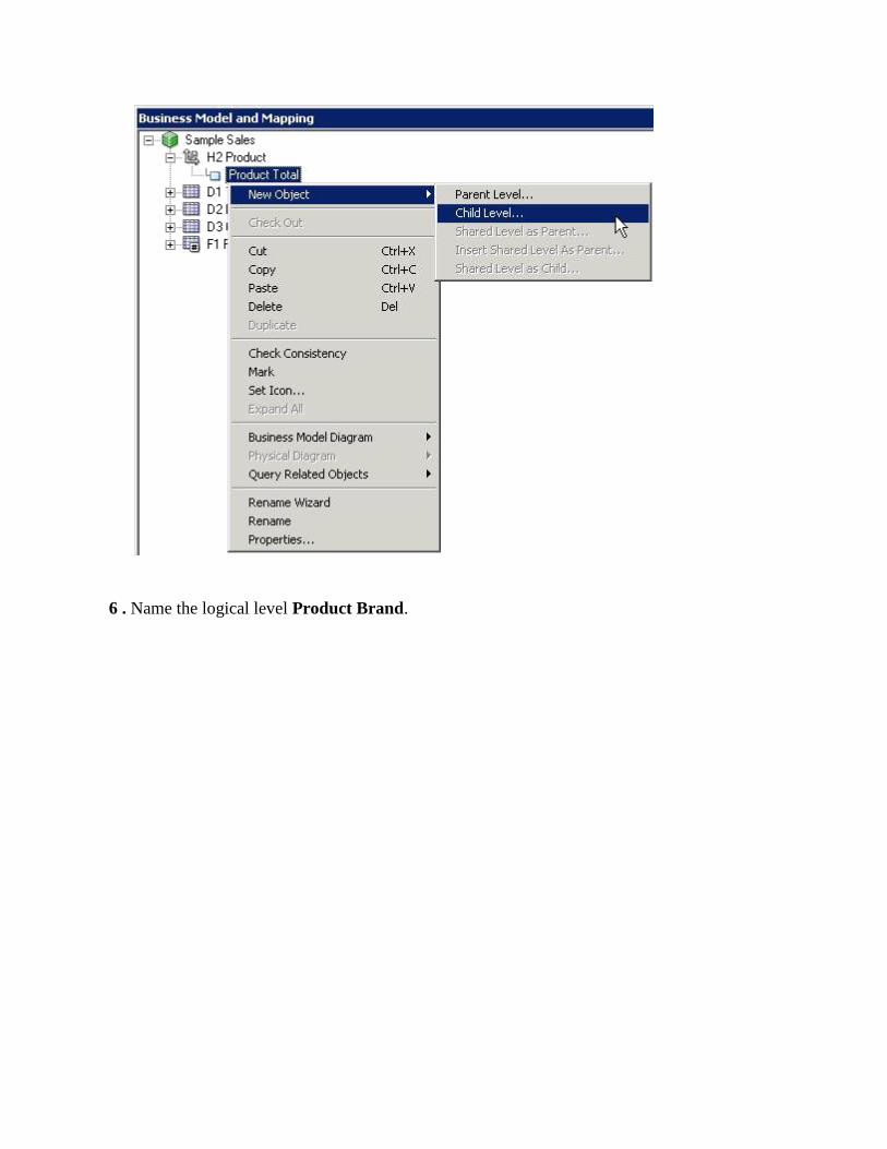
6 . Name the logical level Product Brand.

7 . Click OK to close the Logical Level dialog box. The Product Brand level is added to the
logical dimension. 8 . Repeat the steps to add the following child levels:
Product LOB as a child of Product Brand

Product Type as a child of Product LOB Product Detail as a child of Product Type
Use the screenshot as a guide:
Associate Logical Columns with Logical Levels 1 . Expand the D2 Product logical table.

2 . Drag the Brand column from D2 Product to the Product Brand level in H2 Product.
3 . Continue dragging logical columns from the D2 Product logical table to their corresponding
levels in the H2 Product logical dimension:
Logical Column Logical Level
Lob Product LOB
Type Product Type
Product Product Detail
Prod Key Product Detail
Your results should look similar to the screenshot:

Set Logical Level Keys 1 . Double-click the Product Brand logical level to open the Logical Level dialog box. On the
General tab, notice that the Product LOB child level is displayed.

2 . Click the Keys tab.

3 . Enter Brand for Key Name.

4 . In the Columns field, use the drop down list to select D2 Product.Brand.

5 . Check Use for Display. When this is selected, users can drill down to this column from a higher level.

6 . Set Brand as the Primary key.

7 . Click OK to close the Logical Level dialog box. The icon changes for Brand to show that it is the key for the Product Brand level.
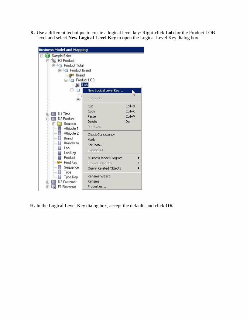
8 . Use a different technique to create a logical level key: Right-click Lob for the Product LOB
level and select New Logical Level Key to open the Logical Level Key dialog box. 9 . In the Logical Level Key dialog box, accept the defaults and click OK.
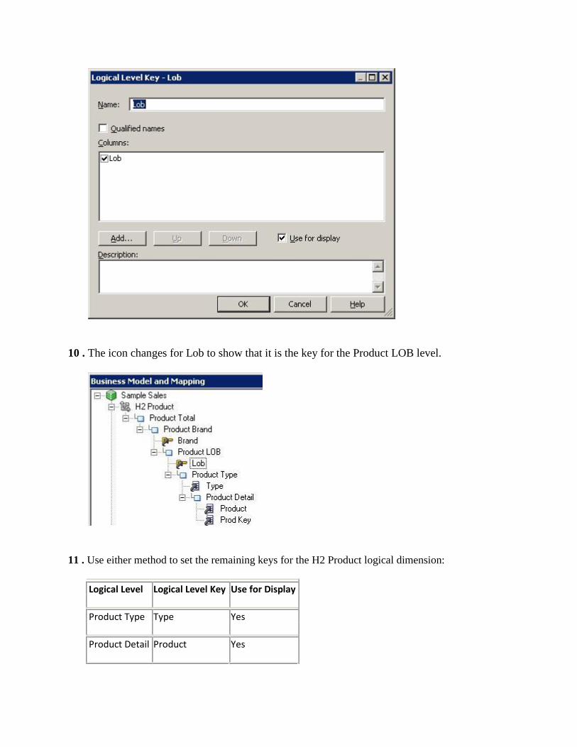
10 . The icon changes for Lob to show that it is the key for the Product LOB level.
11 . Use either method to set the remaining keys for the H2 Product logical dimension:
Logical Level Logical Level Key Use for Display
Product Type Type Yes
Product Detail Product Yes

Product Detail Prod Key No
Your results should look similar to the screenshot: Please note that the Detail level (lowest level of the hierarchy) must have the column that is the logical key of the dimension table associated with it and it must be the key for that level: Prod Key in this example.
12 . Set Prod Key as the primary key for the Product Detail level. Hint: Double-click the level and select the Keys tab.

Create a Logical Dimension for Time 1 . Use a different technique to create a logical dimension for Time. Right-click the D1 Time logical
table and select Create Logical Dimension > Dimension with Level-Based Hierarchy.

2 . A new logical dimension, D1 TimeDim in this example, is automatically added to the business
model.
3 . Rename D1 TimeDim to H1 Time .

4 . Expand H1 Time . Notice that two level were created automatically: D1 Time Total and D1
Time Detail. D1 Time Detail is populated with all of the columns from the D1 Time logical table.

5 . Rename D1 Time Total to Time Total, and rename D1 Time Detail to Time Detail.

6 . Right-click Time Detail and select New Object > Parent Level to open the Logical Level
dialog box.
7 . On the General tab, name the logical level Week, and check Supports rollup to higher level of
aggregation.

8 . Click OK to close the Logical Level dialog box. The Week level is added to the H1 Time logical
dimension. 9 . Repeat the steps to add the remaining logical levels:
Month as a parent of Week
Quarter as a parent of Month
Half as a parent of Quarter

Year as a parent of Half
Your final results should look similar to the screenshot:
Associate Time Logical Columns with Logical Levels 1 . Use a different technique to associate logical columns with logical levels. Drag the logical
columns from the Time Detail logical level (not from the D1 Time logical table) to their corresponding levels in the H1 Time logical dimension. This is a convenient technique when logical columns are buried deep in the business model.
Logical Column Logical Level
Per Name Year Year
Per Name Half Half
Per Name Qtr Quarter Per Name Month Month

Per Name Week Week
Your results should look similar to the screenshot:
2 . Delete all remaining columns from the Time Detail level except for Calendar Date so that only Calendar Date is associated with the Time Detail level. Notice that deleting objects from the hierarchy does not delete them from the logical table in the business model.

3 . Set the logical keys for the H1 Time logical dimension according to the following table:
Logical Level Level Key Use for Display
Year Per Name Year Yes
Half Per Name Half Yes
Quarter Per Name Qtr Yes
Month Per Name Month Yes
Week Per Name Week Yes
Time Detail Calendar Date Yes

Create a Logical Dimension for Customer 1 . Use either technique to create a logical dimension with a level-based hierarchy named H3
Customer for the D3 Customer logical table with the following levels, columns, and keys. Hint: Create the levels first, then double-click a logical column to open the Logical Column dialog box and use the Levels tab to associate the logical column with a logical level.
Level Column Key Use for
Display
Customer Total <none> <none> <none>
Customer Region Region Region Yes
Customer Area Area Area Yes
Customer Country Country Name Country Name Yes
Customer State State Province State Province Yes
Customer City City City Yes
Customer Postal Postal Code Postal Code Yes
Code
Customer Detail Customer Name Customer Name Yes
Customer Customer No

Number Number
Set Customer Total as the grand total level.
Set Customer Number as the primary key for the Customer Detail
level. Your results should look similar to the screenshot:
Set Aggregation Content for Logical Table Sources 1 . Expand D1 Time > Sources.
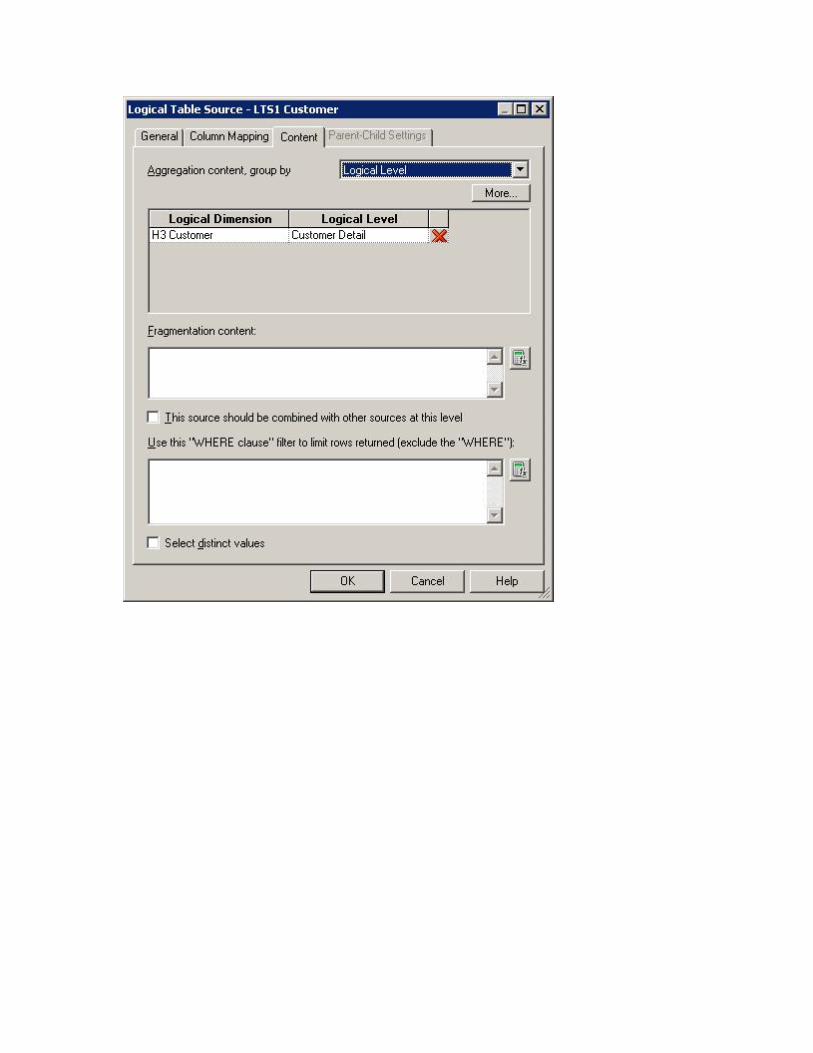
2 . Double-click the LTS1 Time logical table source to open the Logical Table Source dialog box.

3 . Click the Content tab. 4 . Confirm that Aggregation content, group by is set to Logical Level and the logical level is set
to Time Detail for the H1 Time logical dimension.

5 . Click OK to close the Logical Table Source dialog box. 6 . Repeat to verify or set content settings for the remaining logical table sources using the table and
screenshots as a guide:
Logical Table Source Logical Dimension Logical Level
LTS1 Product H2 Product Product Detail
LTS1 Customer H3 Customer Customer Detail
LTS2 Customer Address H3 Customer Customer Detail
LTS1 Revenue H1 Time Time Detail

H2 Product Product Detail
H3 Customer Customer Detail


7 . Save the repository and check global consistency. Fix any errors or warnings before proceeding.
Notice that you did not have to make any changes to the Presentation layer.
8 . Close the repository. Leave the Administration Tool open.
Test Your Work 1 . Return to Fusion Middleware Control and load the BISAMPLE repository. 2 . Return to Oracle BI, which should still be open, and sign in if necessary. 3 . Create the following analysis to test the Product hierarchy.
Products.Brand
Base Facts.Revenue
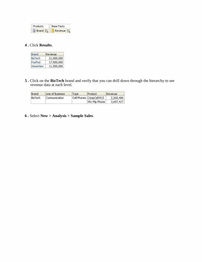
4 . Click Results.
5 . Click on the BizTech brand and verify that you can drill down through the hierarchy to see
revenue data at each level. 6 . Select New > Analysis > Sample Sales.

7 . Click OK to confirm that you want to navigate away from this page.
8 . Create the following analysis:
Time.Per Name Year
Base Facts.Revenue

9 . Click Results and verify that you can drill down through the Time hierarchy.
10 . Repeat the steps and create the following analysis to test the Customers hierarchy:
Customer Regions.Region
Base Facts.Revenue 11 . Click Results and verify that you can drill down through the Customers hierarchy. 12 . Sign out of Oracle BI. Click OK when prompted about navigating away from this page.
Leave the Oracle BI browser page open.
Creating Level-Based Measures
In this set of steps you create level-based measures that calculate total dollars at various levels in the Product hierarchy, and then use a level-based measure to create a share measure.

To create level-based measures and a share measure, you perform the following steps:
Open the Repository in Offline Mode
Create Level-Based Measures
Create a Share Measure
Test Your Work
Open the Repository in Offline Mode 1 . Return to the Administration Tool, which should still be open. If not, select Start > Programs >
Oracle Business Intelligence > BI Administration.
2 . Select File > Open > Offline. 3 . Select BISAMPLE.rpd and click Open. Do not select any BISAMPLE repository with an
extension, for example, BISAMPLE_BI0001.rpd. Recall that these are the repositories that have been loaded into Oracle BI Server memory.
4 . Enter admin123 as the repository password and click OK to open the repository.
Create Level-Based Measures 1 . In the Business Model and Mapping layer, right-click the F1 Revenue table and select New
Object > Logical Column to open the Logical Column dialog box.
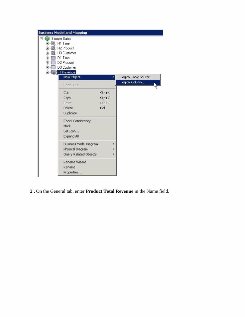
2 . On the General tab, enter Product Total Revenue in the Name field.

3 . Click the Column Source tab.

4 . Select Derived from existing columns using an expression.

5 . Open the Expression Builder.

6 . In the Expression Builder, add Logical Tables > F1 Revenue > Revenue to the expression. Recall that the Revenue column already has a default aggregation rule of Sum.

7 . Click OK to close Expression Builder.
8 . Click the Levels tab.

9 . For the H2 Product logical dimension, select Product Total from the Logical Level drop-down list to specify that this measure should be calculated at the grand total level in the product hierarchy.

10 . Click OK to close the Logical Column dialog box. The Product Total Revenue measure appears in the Product Total level of the H2 Product logical dimension and the F1 Revenue logical fact table.

11 . Repeat the steps to create a second level-based measure:
Name Logical Dimension Logical Level
Product Type Revenue H2 Product Product Type

12 . Expose the new columns to users by dragging Product Total Revenue and Product Type Revenue to the Base Facts presentation table in the Sample Sales subject area in the Presentation layer. You can drag the columns from either the H2 Product logical dimension or the F1 Revenue logical table.

Create a Share Measure 1 . In the Business Model and Mapping layer, right-click the F1 Revenue table and select New
Object > Logical Column to open the Logical Column dialog box.
2 . On the General tab, name the logical column Product Share.

3 . On the Column Source tab, select "Derived from existing columns using an expression."

4 . Open the Expression Builder.

5 . In the Expression Builder, Select Functions > Mathematic Functions > Round.

6 . Click Insert selected item. The function appears in the edit box.

7 . Click Source Number in the formula.

8 . Enter 100* followed by a space.

9 . Insert Logical Tables > F1 Revenue > Revenue.

10 . Using the toolbar, click the Division button. Another set of angle brackets appears, <<expr>>.

11 . Click <<expr>>.

12 . Insert Logical Tables > F1 Revenue > Product Total Revenue. Recall that this is the
total measure for the hierarchy.

13 . Click between the last set of angle brackets, <<Digits>>, and enter 1. This represents
the number of digits of precision with which to round the integer.

14 . Check your work:
Round(100* "Sample Sales"."F1 Revenue"."Revenue" / "Sample Sales"."F1 Revenue"."Product Total Revenue" , 1)
This share measure will allow you to run an analysis that shows how revenue of a specific product compares to total revenue for all products.
15 . Click OK to close the Expression Builder. The formula is visible in the Logical Column
dialog box.

16 . Click OK to close the Logical Column dialog box. The Product Share logical column is added to the business model.

17 . Add the Product Share measure to the Base Facts presentation table.
18 . Save the repository. Check consistency. You should receive the following message.

If there are consistency errors or warnings, correct them before you proceed.
19 . Close the repository.
Test Your Work 1 . Return to Fusion Middleware Control and load the BISAMPLE repository. 2 . Return to Oracle BI, which should still be open, and sign in. 3 . Create the following analysis to test the level-based and share measures.
Products.Product
Base Facts.Revenue
Base Facts.Product Type Revenue
Base Facts.Product Share 4 . For the Product Share column, select Column Properties. 5 . On the Data Format tab, select Override Default Data Format.
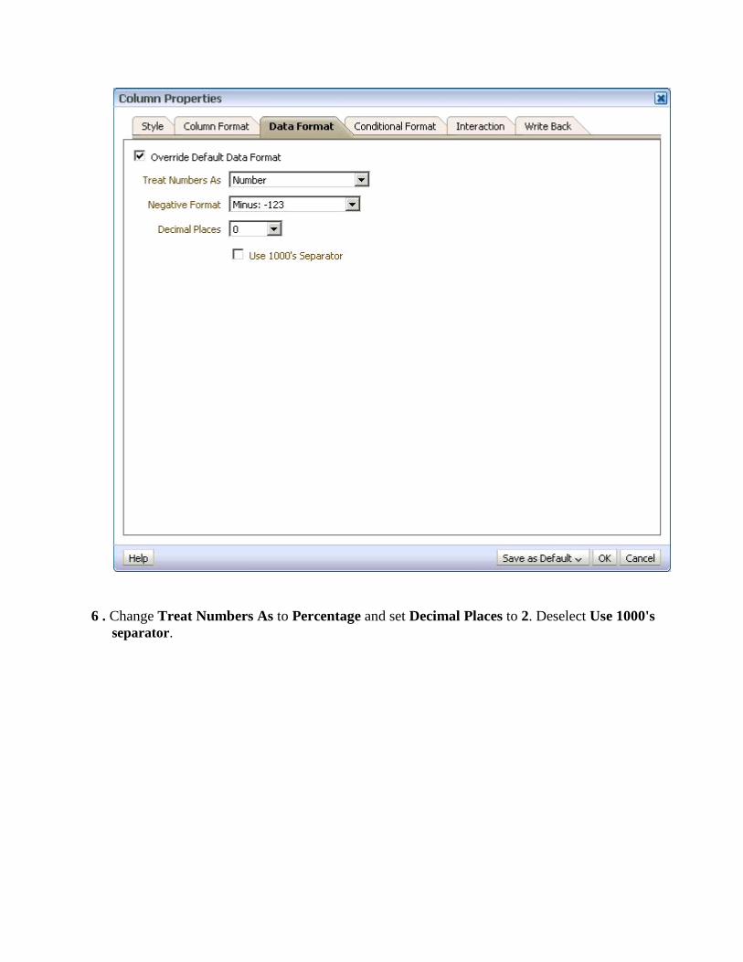
6 . Change Treat Numbers As to Percentage and set Decimal Places to 2. Deselect Use 1000's separator.

7 . Click OK to close the Column Properties dialog box.
8 . Sort Product Share in descending order.

9 . Click Results. Notice that Product Type Revenue returns dollars grouped by Type even though
the query is at a different level than Type; Product in this example. Product Share shows the percent of total revenue for each product sorted in descending order.
10 . Sign out of Oracle BI. 11 . Click OK when you receive the message: Are you sure you want to navigate away from
this page?
Creating Logical Dimensions with Parent-Child Hierarchies
A parent-child hierarchy is a hierarchy of members that all have the same type. This contrasts with level-based hierarchies, where members of the same type occur only at a single level of the hierarchy. The most common real-life occurrence of a parent-child hierarchy is an organizational reporting hierarchy chart, where the following all apply: • Each individual in the organization is an employee.
• Each employee, apart from the top-level managers, reports to a single manager.
• The reporting hierarchy has many levels. In relational tables, the relationships between different members in a parent-child hierarchy are implicitly defined by the identifier key values in the associated base table. However, for each Oracle BI Server parent-child hierarchy defined on a relational table, you must also explicitly define the inter-member relationships in a separate parent-child relationship table.

To create a logical dimension with a parent-child hierarchy, perform the following steps:
Open the Repository in Offline Mode
Import Metadata and Define Physical Layer Objects
Create Logical Table and Logical Columns
Create a Logical Join
Create a Parent-Child Logical Dimension
Define Parent-Child Settings
Create Presentation Layer Objects
Test Your Work
Open the Repository in Offline Mode 1 . Return to the Administration Tool, which should still be open. If not, select Start > Programs >
Oracle Business Intelligence > BI Administration.
2 . Select File > Open > Offline. 3 . Select BISAMPLE.rpd and click Open. Do not select any BISAMPLE repository with an
extension, for example, BISAMPLE_BI0001.rpd. Recall that these are the repositories that have been loaded into Oracle BI Server memory.
4 . Enter admin123 as the repository password and click OK to open the repository.
Import Metadata and Define Physical Layer Objects 1 . In the Physical layer, expand orcl. 2 . Right-click Connection Pool and select Import Metadata to open the Import Wizard.

3 . In the Select Metadata Types screen, accept the defaults and click Next.

4 . In the Select Metadata Objects screen, in the data source view, expand BISAMPLE and select
the following tables for import:
SAMP_EMPL_D_VH
SAMP_EMPL_PARENT_CHILD_MAP
SAMP_EMPL_POSTN_D

5 . Click the Import Selected button to move the tables to the Repository View.

6 . Click Finish to close the Import Wizard.
7 . Confirm that the three tables are visible in the Physical layer of the repository.

8 . Right-click SAMP_EMPL_PARENT_CHILD_MAP and select View Data.

This is an example of a parent-child relationship table with rows that define the inter-member relationships of an employee hierarchy. It includes a Member Key column, which identifies the member (employee); an Ancestor Key, which identifies the ancestor (manager) of the member; a Distance column, which specifies the number of parent-child hierarchy levels from the member to the ancestor; and a Leaf column, which indicates if the member is a leaf member.
9 . Create the following aliases for the tables:
Table Alias
SAMP_EMPL_D_VH D50 Sales Rep
SAMP_EMPL_PARENT_CHILD_MAP D51 Sales Rep Parent Child
SAMP_EMPL_POSTN_D D52 Sales Rep Position

10 . Use the Physical Diagram to create the following physical joins for the alias tables:
"orcl".""."BISAMPLE"."D52 Sales Rep Position"."POSTN_KEY" =
"orcl".""."BISAMPLE"."D50 Sales Rep"."POSTN_KEY"
"orcl".""."BISAMPLE"."D50 Sales Rep"."EMPLOYEE_KEY" = "orcl".""."BISAMPLE"."D51 Sales Rep Parent Child"."ANCESTOR_KEY"
"orcl".""."BISAMPLE"."D51 Sales Rep Parent Child"."MEMBER_KEY" =
"orcl".""."BISAMPLE"."F1 Revenue"."EMPL_KEY"

Create Logical Table and Logical Columns 1 . In the BMM layer, right-click the Sample Sales business model and select New Object >
Logical Table to open the Logical Table dialog box.

2 . On the General tab, name the logical table D5 Sales Rep.

3 . Click OK to add the logical table to the business model.
Notice that the D5 Sales Rep icon has a # sign. This is because you have not yet defined the logical join relationship. When you define the logical join later in this tutorial the icon will change accordingly.
4 . Drag all six columns from D50 Sales Rep in the Physical layer to D5 Sales Rep in the BMM
layer. This action creates logical columns and adds a D50 Sales Rep logical table source to D5 Sales Rep.

5 . Rename the D50 Sales Rep logical table source to LTS1 Sales Rep.
6 . In the Physical layer, expand D52 Sales Rep Position.

7 . Drag POSTN_DESC and POSTN_LEVEL from D52 Sales Rep Position to LTS1 Sales Rep. Note that you are dragging the columns to the logical table source, not the logical table. Dragging to the logical table would create a second logical table source.
8 . Drag DISTANCE from D51 Sales Rep Parent Child to LTS1 Sales Rep. Again, you drag the
column to the logical table source, not the logical table.

9 . Rename the logical columns:
Old Name
POSTN_KEY
TYPE
EMPL_NAME
EMPLOYEE_KEY
HIRE_DT
MGR_ID
POSTN_DESC
New Name
Position Key
Sales Rep Type
Sales Rep Name
Sales Rep Number
Hire Date
Manager Number
Position
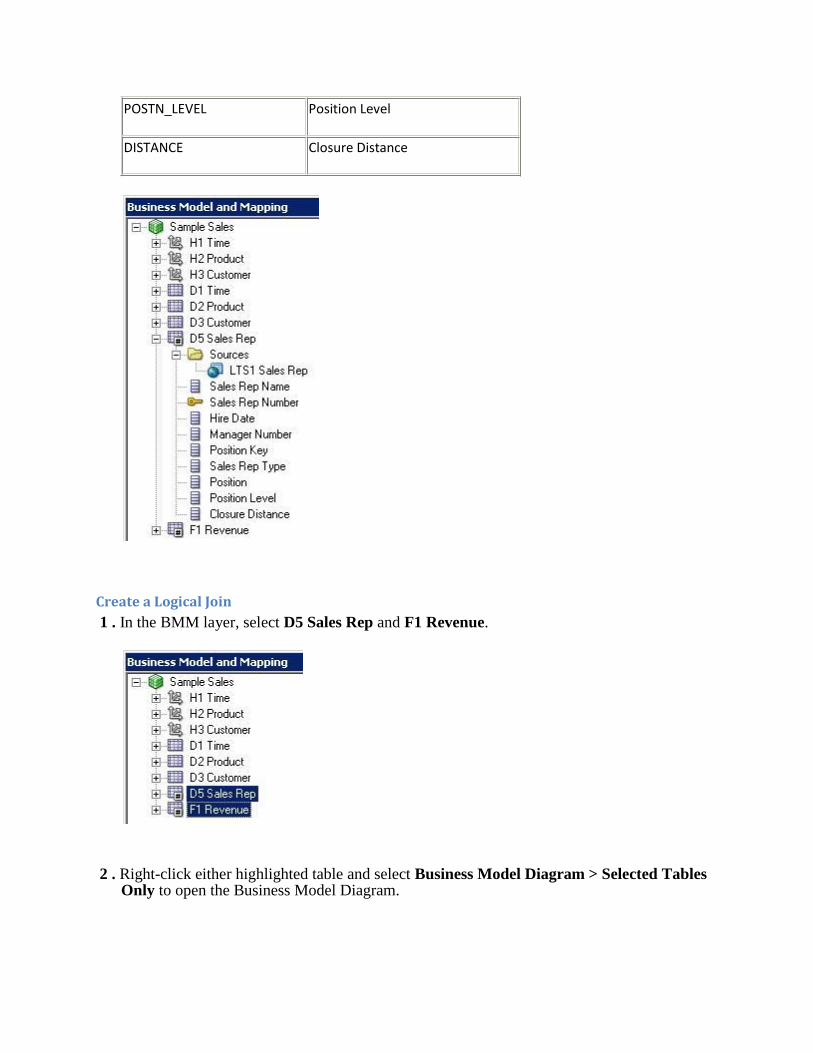
POSTN_LEVEL
DISTANCE
Position Level
Closure Distance
Create a Logical Join 1 . In the BMM layer, select D5 Sales Rep and F1 Revenue.
2 . Right-click either highlighted table and select Business Model Diagram > Selected Tables
Only to open the Business Model Diagram.

3 . Create a logical join between D5 Sales Rep and F1 Revenue with F1 Revenue at the many end of the join.

4 . Close the Business Model Diagram. Notice that the icon has changed for the D5 Sales Rep table. Create a Parent-Child Logical Dimension 1 . Right-click the D5 Sales Rep logical table and select Create Logical Dimension > Dimension
with Parent-Child Hierarchy.

2 . In the Logical Dimension dialog box, on the General tab, name the logical dimension H5 Sales
Rep.

3 . Click Browse next to Member Key. The Browse window shows the physical table and its corresponding key.
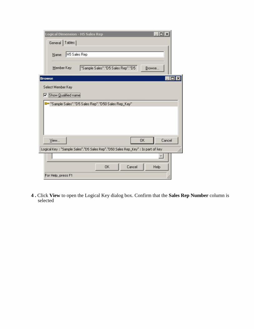
4 . Click View to open the Logical Key dialog box. Confirm that the Sales Rep Number column is selected

5 . Click Cancel to close the Logical Key dialog box.
6 . Click OK to close the Browse window. 7 . Click Browse next to Parent Column. The Browse window shows the columns other than the
member key.

8 . Deselect Show Qualified Names and select Manager Number as the parent column for the parent-child hierarchy.

9 . Click OK to close the Browse window, but do not close the Logical Dimension dialog box.
Define Parent-Child Settings 1 . Click Parent-Child Settings to display the Parent-Child Relationship Table Settings dialog box.
Note that at this point the Parent-Child Relationship Table is not defined.

For each parent-child hierarchy defined on a relational table, you must explicitly define the inter-member relationships in a separate parent-child relationship table. In the process of creating the parent-child relationship table, you may choose one of the following options: 1. Select a previously-created parent-child relationship table. 2. Use a wizard that will generate scripts to create and populate the parent-child relationship table. In the next set of steps you select a previously created and populated parent-child relationship table.
For your information only: To start the wizard you would click the Create Parent-Child Relationship Table button. The wizard creates the appropriate repository metadata objects and generates SQL scripts for creating and populating the parent-child relationship table. At the end of the wizard, Oracle BI Server stores the scripts into directories chosen during the wizard session. The scripts can then be run against the database to create and populate the parent-child relationship table. Running the wizard is not necessary in this tutorial because the parent-child relationship table is already created and populated.
2 . Click the Select Parent-Child Relationship Table button to open the Select Physical Table dialog box.

3 . In the Select Physical Table dialog box, select the D51 Sales Rep Parent Child alias you created.
4 . The D51 Sales Rep Parent Child alias is now displayed in the Parent-Child Relationship Table column.

5 . In the Parent-Child Table Relationship Column Details section, set the appropriate columns:
Member Key
Parent Key
MEMBER_KEY
ANCESTOR_KEY
Relationship Distance DISTANCE
Leaf Node Identifier IS_LEAF

Explanation:
Member Key identifies the member. Parent Key identifies an ancestor of the member, The ancestor may be the parent of the member, or a higher-level ancestor. Relationship Distance specifies the number of parent-child hierarchical levels from the member to the ancestor. Leaf Node Identifier indicates if the member is a leaf member (1=Yes, 0=No).
6 . Click OK to close the Parent-Child Relationship Table Settings dialog box.

7 . Click OK to close the Logical Dimension dialog box.
8 . Right-click H5 Sales Rep and select Expand All. Note that a parent-child logical dimension has only two levels.
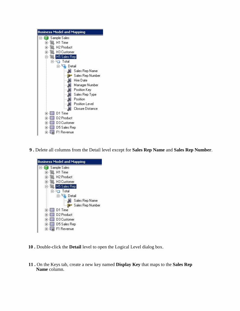
9 . Delete all columns from the Detail level except for Sales Rep Name and Sales Rep Number. 10 . Double-click the Detail level to open the Logical Level dialog box. 11 . On the Keys tab, create a new key named Display Key that maps to the Sales Rep
Name column.
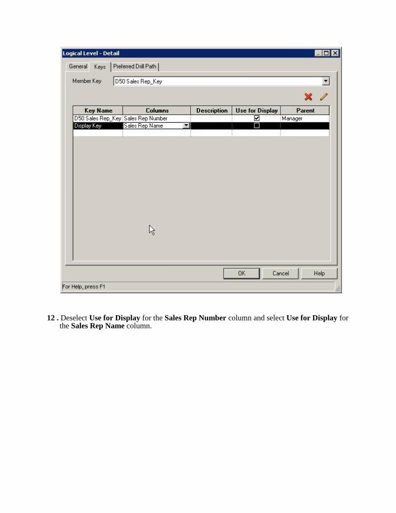
12 . Deselect Use for Display for the Sales Rep Number column and select Use for Display for the Sales Rep Name column.

13 . Make sure that Member Key is still set to D50 Sales Rep_Key.

14 . Click OK to close the Logical Level dialog box.

15 . Expand F1 Revenue > Sources and double-click LTS1 Revenue to open the Logical
Table Source dialog box. 16 . On the Content tab, set the logical level to Detail for the H5 Sales Rep logical dimension.

17 . Click OK to close the Logical Table Source dialog box.

Create Presentation Layer Objects 1 . Drag the D5 Sales Rep logical table from the BMM layer to the Sample Sales subject area in the
Presentation layer.

2 . Rename the D5 Sales Rep presentation table to Sales Reps. 3 . Move the Sales Reps presentation table above the Base Facts table.

4 . Expand the Sales Reps presentation table and notice that the H5 Sales Rep parent-child logical
dimension is automatically included as a presentation hierarchy.
5 . Double-click the H5 Sales Rep presentation hierarchy to open the Presentation Hierarchy dialog

box.
6 . On the Display Columns tab, confirm that Sales Rep Name is set as the display column.
7 . Click OK to close the Presentation Hierarchy dialog box.
8 . Save the repository and check consistency. Fix any errors or warnings before proceeding.
9 . Close the repository. Leave the Administration Tool open.
Test Your Work 1 . Return to Fusion Middleware Control and load the BISAMPLE repository.
2 . Return to Oracle BI, which should still be open, and sign in.
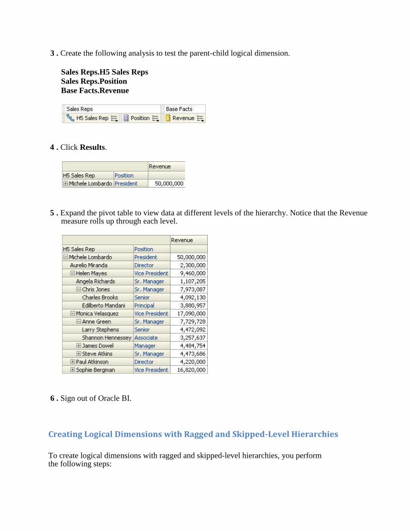
3 . Create the following analysis to test the parent-child logical dimension.
Sales Reps.H5 Sales Reps
Sales Reps.Position
Base Facts.Revenue 4 . Click Results.
5 . Expand the pivot table to view data at different levels of the hierarchy. Notice that the Revenue
measure rolls up through each level. 6 . Sign out of Oracle BI.
Creating Logical Dimensions with Ragged and Skipped-Level Hierarchies
To create logical dimensions with ragged and skipped-level hierarchies, you perform the following steps:

Import Metadata and Define Physical Layer Objects
Create Logical Table and Logical Columns
Create a Ragged/Skipped Levels Logical Dimension
Create Presentation Layer Objects
Test Your Work
Import Metadata and Define Physical Layer Objects 1 . Open the BISAMPLE repository in offline mode.
2 . In the Physical layer, expand orcl.
3 . Right-click Connection Pool and select Import Metadata to open the Import Wizard.

4 . In the Select Metadata Types screen, accept the defaults and click Next.

5 . In the Select Metadata Objects screen, in the data source view, expand BISAMPLE.
6 . In the data source view, select the SAMP_PRODUCTS_DR table for import:

7 . Click the Import Selected button to move the table to the Repository View. 8 . Expand BISAMPLE in the Repository View and confirm that the SAMP_PRODUCT_DR
table is visible.

9 . Click Finish to close the Import Wizard.
10 . Confirm that the SAMP_PRODUCT_DR table is visible in the Physical layer of the repository.

11 . Create the following alias for the table: D20 Product

12 . Use the Physical Diagram to create the following physical join for the alias table:
"orcl".""."BISAMPLE"."D20 Product"."PROD_KEY" = "orcl".""."BISAMPLE"."F1
Revenue"."PROD_KEY"

13 . Right-click D20 Product and select View Data.

Notice there are skipped levels in the hierarchy. For example, brand A - Brand2 has a NULL value for LOB for the product D - Product 8.
14 . Close View Data.
Create Logical Table and Logical Columns 1 . Drag D20 Product from the Physical layer to the Sample Sales business model in the BMM
layer to create a D20 Product logical table. The logical join to F1 Revenue is created automatically based on the join in the Physical layer.

2 . Rename the D20 Product logical columns:
Old Name New Name
BRAND Brand
LOB LOB
PROD_DSC Product
PROD_KEY Product Number
Type Product Type

3 . Rename the D20 Product logical table source to LTS1 Product (Ragged) Create a Ragged/Skipped Level Logical Dimension 1 . Right-click the D20 Product logical table and select Create Logical Dimension > Dimension
with Level-Based Hierarchy to automatically create a logical dimension named D20

ProductDim.

2 . Rename D20 ProductDim to H20 Product.
3 . Double-click the H20 Product logical dimension to open the Logical Dimension dialog box. 4 . On the General tab, select both Ragged and Skipped Levels.

5 . Click OK to close the Logical Dimension dialog box.
6 . Expand H20 Product.

7 . Create the following hierarchy:
Level Column Key Use for Display
Product Total <none> <none> <none>
Product Brand Brand Brand Yes
Product LOB LOB LOB Yes
Product Type Product Type Product Type Yes
Product Product Product Yes Product Detail Product Number Product Number Yes

Create Presentation Layer Objects
1 . Drag the D20 Product logical table to the Sample Sales subject area in the Presentation layer.
2 . In the Presentation layer, rename D20 Product to Products (Ragged) and move Products

(Ragged) to appear after Products.
3 . Expand Products (Ragged) and notice that the H20 Product logical dimension is automatically added to the Presentation layer.
4 . Save the repository and check consistency. Fix and errors or warnings before proceeding.
5 . Close the repository. Leave the Administration Tool open.
Test Your Work
1 . Return to Fusion Middleware Control and load the BISAMPLE repository.

2 . Return to Oracle BI, which should still be open, and sign in.
3 . Create the following analysis to test the ragged / skipped level hierarchy:
Products (Ragged).Brand
Products (Ragged).LOB
Products (Ragged).Product Type
Products (Ragged).Product
Base Facts.Revenue 4 . Click Results.
The results display correctly even though there are skipped levels (levels with NULL values) and ragged levels (leaves with varying depth).
5 . Sign out of Oracle BI.

Using Aggregates
In this set of steps you set up and use aggregate tables to improve query performance. Aggregate tables store pre-computed results, which are measures that have been aggregated (typically summed) over a set of dimensional attributes. Using aggregate tables is a popular technique for speeding up query response times in decision support systems. This eliminates the need for run-time calculations and delivers faster results to users. The calculations are done ahead of time and the results are stored in the tables. Aggregate tables typically have many fewer rows than the non-aggregate tables and, therefore, processing is faster.
To set up and use aggregate tables, perform the following steps:
Import Metadata
Create New Logical Table Sources
Set Aggregate Content
Test Your Work
Import Metadata 1 . Return to the Administration Tool and open the BISAMPLE repository in offline mode.
1 . In the Physical layer, expand orcl.
2 . Right-click Connection Pool and select Import Metadata to open the Import Wizard.
3 . In the Select Metadata Types screen, select Views and click Next.

4 . In the Select Metadata Objects screen, in the data source view, expand BISAMPLE.
5 . In the data source view, select the following for import:
SAMP_REVENUE_FA2
SAMP_TIME_QTR_D

6 . Click the Import Selected button to move the objects to the Repository View.
7 . Expand BISAMPLE in the Repository View and confirm that the objects are visible.

8 . Click Finish to close the Import Wizard.
9 . Confirm that the objects are visible in the Physical layer of the repository.

10 . Create the following aliases:
Table Alias
SAMP_REVENUE_FA2 F2 Revenue Aggregate
SAMP_TIME_QTR_D D1 Time Quarter Grain

11 . Right-click F2 Revenue Aggregate and select View Data. F2 Revenue Aggregate stores aggregated fact information for revenue and units at the quarter and product grain.

12 . Right-click D1 Time Quarter Grain and select View Data. D1 Time Quarter Grain stores
time data at the quarter grain. It stores one record for each quarter beginning with Q4 2006 and ending with Q4 2011.
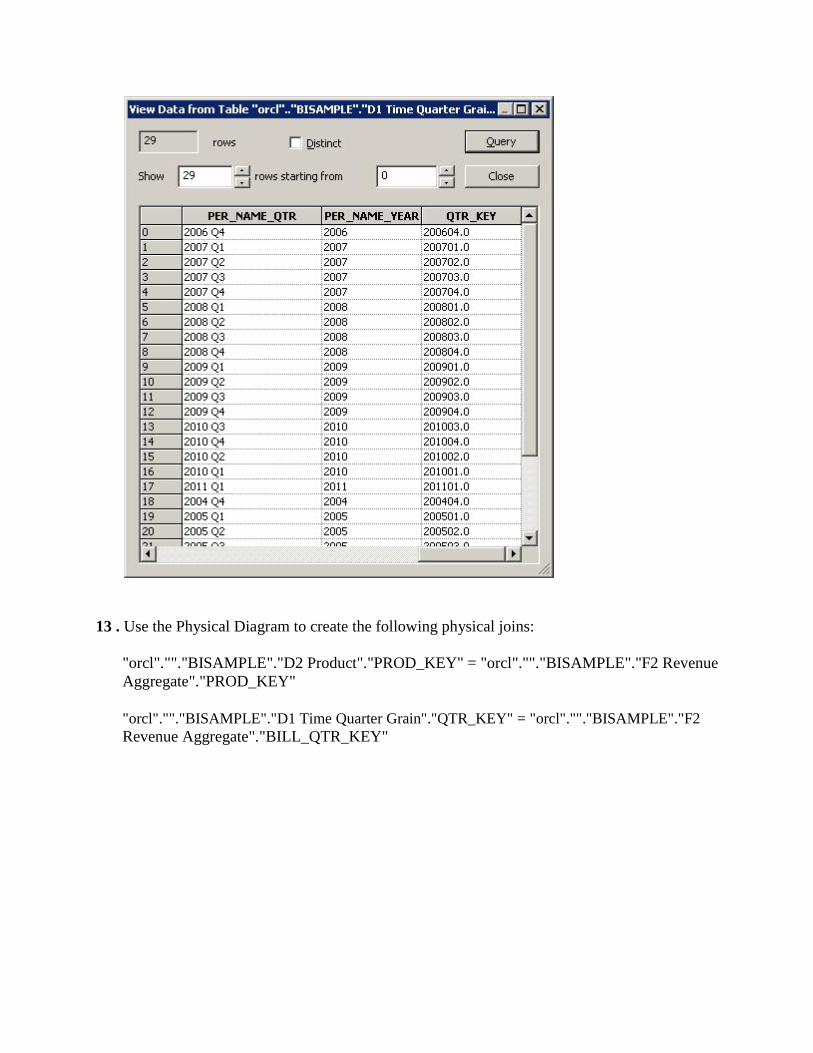
13 . Use the Physical Diagram to create the following physical joins:
"orcl".""."BISAMPLE"."D2 Product"."PROD_KEY" = "orcl".""."BISAMPLE"."F2 Revenue
Aggregate"."PROD_KEY"
"orcl".""."BISAMPLE"."D1 Time Quarter Grain"."QTR_KEY" = "orcl".""."BISAMPLE"."F2 Revenue Aggregate"."BILL_QTR_KEY"

Create New Logical Table Sources 1 . In the Physical layer, expand D1 Time Quarter Grain.

2 . In the BMM layer, expand D1 Time.
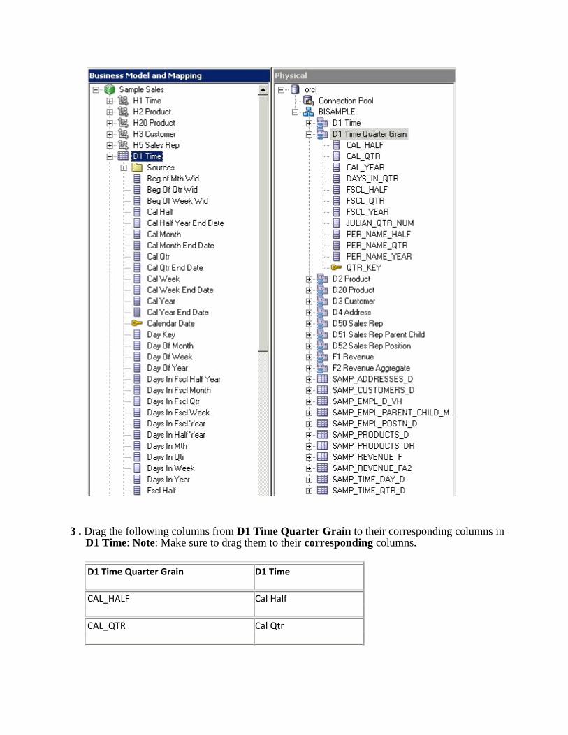
3 . Drag the following columns from D1 Time Quarter Grain to their corresponding columns in D1 Time: Note: Make sure to drag them to their corresponding columns.
D1 Time Quarter Grain D1 Time
CAL_HALF Cal Half
CAL_QTR Cal Qtr

CAL_YEAR Cal Year
DAYS_IN_QTR Days in Qtr
JULIAN_QTR_NUM Julian Qtr Num
PER_NAME_HALF Per Name Half
PER_NAME_QTR Per Name Qtr
PER_NAME_YEAR Per Name Year
This action creates a new logical table source named D1 Time Quarter Grain for D1 Time.
4 . Rename the D1 Time Quarter Grain logical table source to LTS2 Time Quarter Grain.

5 . Double-click LTS2 Time Quarter Grain to open the Logical Table Source dialog box. 6 . On the Column Mapping tab make sure show mapped columns is selected and note the column
mappings. The logical columns now map to columns in two physical tables: D1 Time and D1 Time Quarter Grain.

7 . Click OK to close the Logical Table Source dialog box.
8 . In the Physical layer expand F2 Revenue Aggregate.

9 . In the BMM layer expand F1 Revenue.
10 . Drag the following physical columns from F2 Revenue Aggregate to their
corresponding logical columns in F1 Revenue: Note: Do not add them as new columns.

F2 Revenue Aggregate F1 Revenue
UNITS Units
REVENUE Revenue
This action creates a new logical table source named F2 Revenue Aggregate for F1 Revenue.
11 . Rename the F2 Revenue Aggregate logical table source to LTS2 Revenue Aggregate.

12 . Double-click LTS2 Revenue Aggregate to open the Logical Table Source dialog box. 13 . On the Column Mappings tab make sure show mapped columns is selected and note the
column mappings. The Revenue and Units logical columns now map to columns in two physical tables: F1 Revenue and F2 Revenue Aggregate.
14 . Leave the Logical Table Source - LTS2 Revenue Aggregate dialog box open.

Set Aggregate Content 1 . Click the Content tab.
2 . Set the following logical levels for the logical dimensions:
Logical Dimension Logical Level
H1 Time Quarter
H2 Product Product Total
H20 Product Product Total
H3 Customer Customer Total
H5 Sales Rep Total

Explanation: You are setting aggregation content for the fact table to the corresponding levels in the dimension hierarchies. In a subsequent step, you set similar levels for the aggregate logical table source for the Time dimension. Note that all levels are set to the total level except for the H1 Time logical dimension, which is set to Quarter. The result is, when a user queries against a particular level, Oracle BI Server will “know” to access the aggregate tables instead of the detail tables.
For example, if a user queries for total sales by product by quarter, the server will access the F2 Revenue Aggregate fact table and the corresponding aggregate dimension table, D1 Time Quarter Grain. If a user queries for a level lower than the level specified here, for example Month instead of Quarter, then the server will access the detail tables (F1 Revenue and D1 Time). If a user queries for higher level (year instead of quarter) the aggregate tables will be used, because whenever a query is run against a logical level or above, the aggregate tables are used.
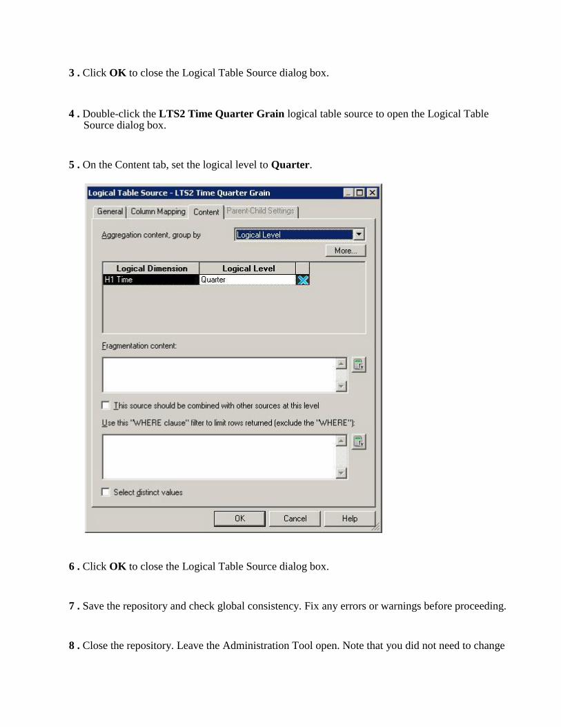
3 . Click OK to close the Logical Table Source dialog box. 4 . Double-click the LTS2 Time Quarter Grain logical table source to open the Logical Table
Source dialog box.
5 . On the Content tab, set the logical level to Quarter. 6 . Click OK to close the Logical Table Source dialog box.
7 . Save the repository and check global consistency. Fix any errors or warnings before proceeding.
8 . Close the repository. Leave the Administration Tool open. Note that you did not need to change

the Presentation layer. You made changes in the business model that impact how queries are processed and which sources are accessed. However, the user interface remains the same, so there is no need to change the Presentation layer. Oracle BI Server will automatically use the appropriate sources based on the user query.
Test Your Work 1 . Return to Fusion Middleware Control Enterprise Manager and load the BISAMPLE
repository.
2 . Return to Oracle BI, which should still be open, and sign in.
3 . Create the following analysis to test the aggregate tables.
Time.Per Name Qtr
Base Facts.Revenue 4 . Click Results. 5 . Leave Oracle BI open.
6 . Use FMW Control or the Administration link to check the query log.

7 . Inspect the log. Notice that the query uses the expected tables: D1 Time Quarter Grain and F2
Revenue Aggregate.
8 . Return to Oracle BI.
9 . Click New > Analysis > Sample Sales.
10 . Create the following analysis to test the aggregate tables.
Time.Per Name Year
Base Facts.Revenue 11 . Click Results.

12 . Check the query log. Hint: If you check the log using FMW Control, click the Refresh button
to refresh the log.
13 . Inspect the log. Notice that the query uses the same tables: D1 Time Quarter Grain and F2
Revenue Aggregate. This is because Per Name Year is at a higher level than Per Name Quarter in the logical dimension hierarchy, so the aggregate tables are still used.
14 . Return to Oracle BI.
15 . Click New > Analysis > Sample Sales.
16 . Create one more analysis to test the aggregate tables.
Time.Per Name Month
Base Facts.Revenue 17 . Click Results.

18 . Inspect the log. Notice that this time the query uses the detail tables: D1 Time and F1
Revenue. This is because the requested data (revenue by month) is at a lower level than what is contained in the aggregate tables. The aggregate tables do not contain the data and, therefore, the detail tables are used in the query. This aggregate navigation is controlled by the aggregate content levels you set in the logical table sources.
19 . Sign out of Oracle BI.

Using Initialization Blocks and Variables
You can use variables in a repository to streamline administrative tasks and modify metadata content dynamically to adjust to a changing data environment. A variable has a single value at any point in time. Variables can be used instead of literals or constants in the Expression Builder in the Administration Tool or in end-user analyses. At run time, Oracle BI Server substitutes the value of the variable.
In this set of steps you create a new initialization block, Current Periods, and three new dynamic repository variables—CurrentYear, CurrentMonth, and CurrentDay. You then use the variables as column filters in an Oracle BI analysis. You use the Variable Manager in the Administration Tool to define variables and initialization blocks.
To set up and use initialization blocks and variables, perform the following steps:
Create an Initialization Block
Create Variables
Test Your Work
Create an Initialization Block 1 . Open the BISAMPLE repository in offline mode.
2 . Select Manage > Variables to open the Variable Manager. 3 . Select Action > New > Repository > Initialization Block.

4 . Name the initialization block Current Periods. 5 . Click the Edit Data Source button to open the Repository Variable Initialization Block Data
Source dialog box.

6 . Click the Browse button to open the Select Connection Pool dialog box.

7 . Double-click the Connection Pool object to select it.

The connection pool is added.

8 . Enter the following SQL to determine the value of the current day, month, and year by finding
the maximum value of the period key (BILL_DAY_DT) in the fact table:
SELECT CALENDAR_DATE, PER_NAME_MONTH, PER_NAME_YEAR FROM BISAMPLE.SAMP_TIME_DAY_D WHERE CALENDAR_DATE = (SELECT MAX(BILL_DAY_DT) FROM BISAMPLE.SAMP_REVENUE_F)
9 . Click Test and confirm the expected results are returned. In this example, the results are determined by the data in the sample database used for this tutorial, which holds data through December 2010.

10 . Close the Results window. 11 . Click OK to close the Repository Variable Initialization Block Data Source dialog box.
Check your work:

Create Variables 1 . Click Edit Data Target to open the Repository Variable Initialization Block Variable Target
dialog box.
2 . Use the New button to create three new variables: CurrentDay, CurrentMonth, CurrentYear.
The order is important. The value returned from the first column in the initialization block SQL, CALENDAR_DATE, is assigned to the CurrentDay variable. The value of the second column, PER_NAME_MONTH, is assigned to CurrentMonth (the second variable), and the value of the third column, PER_NAME_YEAR, is assigned to CurrentYear (the third variable). If necessary, use the Up and Down buttons to arrange the variables.

3 . Click OK to close the Repository Variable Initialization Block Variable Target dialog box. 4 . Leave the default refresh interval set to every hour. This means that the variables will be
reinitialized every hour.

5 . Click the Test button and check the results:

In this example, the results are determined by the data in the sample database used for this tutorial, which holds data through December 2010.
6 . Close the Results window.
7 . Click OK to close the Repository Variable Initialization Block dialog box.
8 . Check your work in the Variable Manager:

9 . Close the Variable Manager.
10 . Save the repository and check consistency. Fix any errors or warnings before proceeding.
11 . Close the repository. Leave the Administration Tool open.
Test Your Work 1 . Return to Fusion Middleware Control and load the BISAMPLE repository.
2 . Return to Oracle BI and sign in.
3 . Create the following analysis to test the variables.
Time.Per Name Year

Time.Per Name Month
Time.Calendar Date
Base Facts.Revenue 4 . Click Filter for the Per Name Year column. The New Filter dialog box opens. 5 . Select Add More Options > Repository Variable.
6 . In the Repository Variable field, enter CurrentYear to create a filter for the Per Name Year column using the CurrentYear repository variable.
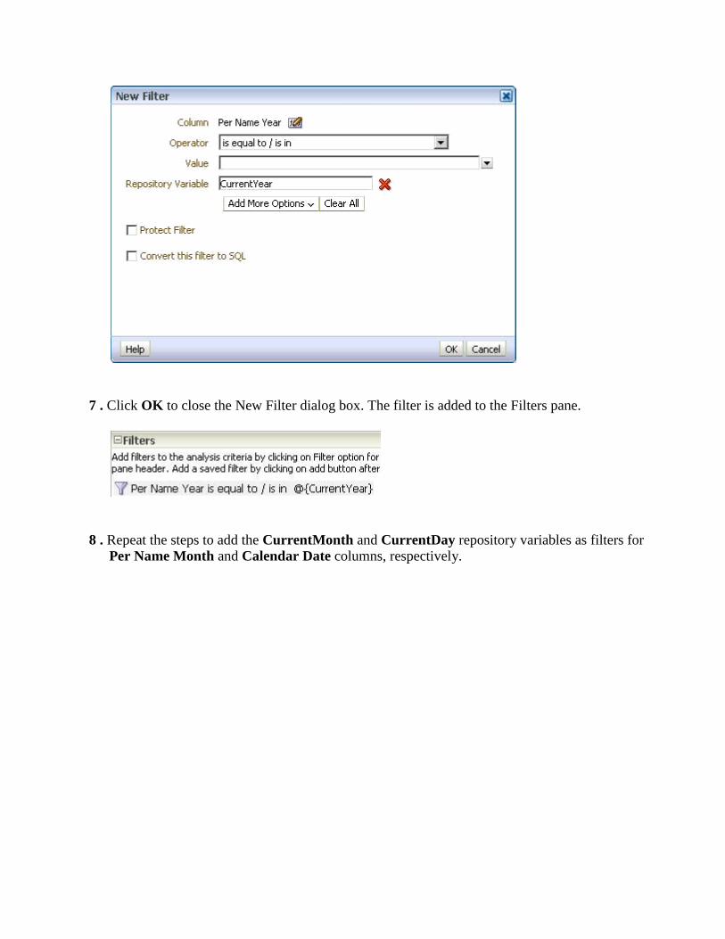
7 . Click OK to close the New Filter dialog box. The filter is added to the Filters pane.
8 . Repeat the steps to add the CurrentMonth and CurrentDay repository variables as filters for Per Name Month and Calendar Date columns, respectively.

9 . Click Results and confirm that data only for the current year, month, and day is returned (based
on the sample data set).
10 . Sign out of Oracle BI.
Creating Time Series Measures
In this topic you create time series calculation measures using Oracle BI time series functions.
Time series functions include AGO, TODATE, and PERIODROLLING. These functions let you use Expression Builder to call a logical function to perform time series calculations instead of creating aliases for physical tables and modeling logically. The time series functions calculate AGO, TODATE, and PERIODROLLING functions based on the calendar tables in your data warehouse, not on standard SQL date manipulation functions.
To create time series measures, you perform the following steps:
Identify a Logical Dimension as a Time Dimension
Identify Level Keys as Chronological Keys
Create a Measure Using the AGO Function
Create a Measure Using the TODATE Function
Create a Measure Using the PERIODROLLING Function
Test Your Work
Identify a Logical Dimension as a Time Dimension
1 . Return to the Administration Tool and open the BISAMPLE repository in offline mode. 2 . In the BMM layer, double-click the H1 Time logical dimension to open the Logical Dimension
dialog box.

3 . In the Structure section, select Time.
Time series functions operate on time-oriented dimensions. To use these functions on a

particular dimension, you must designate the dimension as a Time dimension.
4 . Click OK to close the Logical Dimension dialog box.
Identify Level Keys as Chronological Keys 1 . Expand the H1 Time logical dimension and double-click the Time Detail level to open the
Logical Level dialog box.
2 . Click the Keys tab.

3 . Select the Chronological Key check box for Calendar Date. 4 . Click OK to close the Logical Level dialog box.
5 . Repeat and set chronological keys for the following levels:
Logical Level Chronological Key
Year Per Name Year
Half Per Name Half Quarter Per Name Qtr

Month Per Name Month
Week Per Name Week
It is best practice to designate a chronological key for every level of a time logical dimension.
Create a Measure Using the AGO Function
1 . Right-click the F1 Revenue logical table and select New Object > Logical Column.
2 . On the General tab, name the column Month Ago Revenue.

3 . On the Column Source tab, select "Derived from existing columns using an expression." 4 . Open the Expression Builder.
5 . Select Functions > Time Series Functions > Ago.

6 . Double-click Ago or click Insert selected item to add the Ago function to the Expression Builder.

7 . Click <<Measure>>in the expression.

8 . Select Logical Tables > F1 Revenue and then double-click Revenue to add it to the expression.

9 . Click <<Level>> in the expression.

10 . Select Time Dimensions > H1 Time and then double-click Month to add it to the expression.

11 . Click <<Number of Periods>> and enter 1. The Ago function will calculate the Revenue
value one month before the current month.

12 . Click OK to close the Expression Builder. Check your work in the Logical Column dialog box:

13 . Click OK to close the Logical Column dialog box. The Month Ago Revenue time series measure is added to the F1 Revenue logical table.
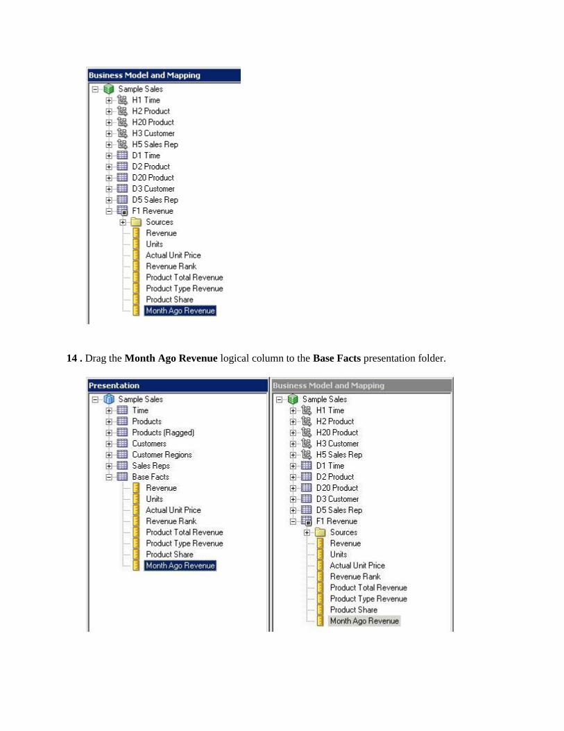
14 . Drag the Month Ago Revenue logical column to the Base Facts presentation folder.

Create a Measure Using the TODATE Function
1 . Right-click the F1 Revenue logical table and select New Object > Logical Column.
2 . On the General tab, name the new logical column Year To Date Revenue. 3 . On the Column Source tab, select "Derived from existing columns using an expression."

4 . Open the Expression Builder.
5 . Select Functions > Time Series Functions and double-click ToDate to insert the expression.

6 . Click <<Measure>> in the expression.

7 . Select Logical Tables > F1 Revenue and then double-click Revenue to add it to the expression.

8 . Click <<Level>> in the expression.

9 . Select Time Dimensions > H1 Time and then double-click Year to add it to the expression.

10 . Click OK to close the Expression Builder.
11 . Check your work in the Logical Column dialog box:

12 . Click OK to close the Logical Column dialog box.
13 . Drag the Year To Date Revenue logical column to the Base Facts presentation folder.

Create a Measure Using the PERIODROLLING Function
1 . Right-click the F1 Revenue logical table and select New Object > Logical Column.
2 . On the General tab, name the new logical column Revenue 3-Period Rolling Sum.

3 . On the Column Source tab, select "Derived from existing columns using an expression."

4 . Open the Expression Builder. 5 . Select Functions > Time Series Functions and double-click PeriodRolling to insert the
expression.

6 . Click <<Measure>> in the expression.

7 . Select Logical Tables > F1 Revenue and then double-click Revenue to add it to the expression.

8 . Click <<Starting Period Offset>> in the expression.

9 . Enter -2. This identifies the first period in the rolling aggregation.
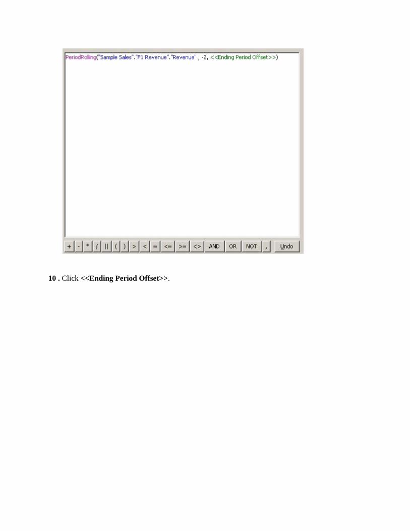
10 . Click <<Ending Period Offset>>.

11 . Enter 0. This identifies the last period in the rolling aggregation.

These integers are the relative number of periods from a displayed period. In this example, if the query grain is month, the 3 month rolling sum starts two months in the past (-2) and includes the current month (0).
12 . Click OK to close the Expression Builder.
13 . Check your work in the Logical Column dialog box:

14 . Click OK to close the Logical Column dialog box.
15 . Drag the Revenue 3-Period Rolling Sum logical column to the Base Facts presentation folder.

16 . Save the repository and check consistency. Fix any errors or warnings before you proceed.
17 . Close the repository. Leave the Administration Tool open.
Test Your Work
1 . Return to Fusion Middleware Control and load the BISAMPLE repository.
2 . Return to Oracle BI and sign in.
3 . Create the following analysis to test AGO and TODATE functions:
Time.Per Name Month
Time.Per Name Year
Base Facts.Revenue
Base Facts.Month Ago Revenue

Base Facts.Year to Date Revenue
4 . Set the following filter for the analysis:
Per Name Year is equal to / is in 2008.
5 . For the Per Name Year column, select Column Properties > Column Format > Hide. This
will prevent Per Name Year from displaying in the analysis results.

6 . Sort Per Name Month in ascending order. 7 . Click Results.
Month Ago Revenue displays revenue from the previous month. Year To Date Revenue calculates a running sum of revenue for the year on a monthly basis.
8 . Create the following new analysis and filter to test the PERIODROLLING function at the month
grain:
Time.Per Name Month
Time.Per Name Year
Base Facts.Revenue
Base Facts.Revenue 3-Period Rolling Sum
Per Name Year is equal to / is in 2008 9 . For the Per Name Year column, select Column Properties > Column Format > Hide. This

will prevent Per Name Year from displaying in the analysis results.
10 . Sort Per Name Month in ascending order. 11 . Click Results.

Revenue 3-Period Rolling Sum is calculated based on the month grain. 12 . Create the following new analysis and filter to test the PERIODROLLING function at the
year grain:
Time.Per Name Year
Base Facts.Revenue
Base Facts.Revenue 3-Period Rolling Sum 13 . Sort Per Name Year in ascending order. 14 . Click Results.
Revenue 3-Period Rolling Sum is calculated based on the year grain. A measure with the PERIODROLLING function calculates results based on the query grain.