Representing Maps in Computers

BAE 599 Topics in Agriculture Engineering: Precision

Agriculture

S.A. ShearerBiosystems and Agricultural Engineering

University of Kentucky

Geographic Information System (GIS)Database that permits the collection and storage of spatial data along with associated attribute data for the purposes of retrieval, analysis, synthesis, and display to promote understanding and assist in decision making.GIS is the merger of attribute and a geographic databases.GIS is a spatial decision support system (not a decision making system).

Storing Spatial Data in a ComputerFeatures on the earth’s surface are mapped to two-dimensional maps as points, lines and areas.

Points are a single x-y locationLines (arcs) are a series of x-y pointsAreas are a series of points that define arcs that enclose an area forming a polygon

Points, Arcs, and Polygons

TopologyMathematical procedure for explicitly defining spatial relationships; relationships are expressed as a list of featuresAllows computers to store data efficiently thereby enabling faster processing of larger data setsMajor topological concepts:

Arcs connect to each other at nodes (connectivity)Arcs are connected to surround an area defined a polygon (area definition)Arcs have direction and left and right sides (contiguity).

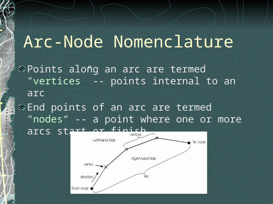
Arc-Node Nomenclature

Points along an arc are termed "vertices” -- points internal to an arcEnd points of an arc are termed "nodes“ -- a point where one or more arcs start or finish.

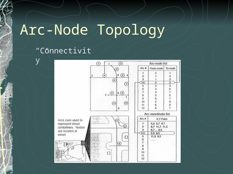
Arc-Node Topology“Connectivity”

Polygon-Arc Topology“Area Definition”

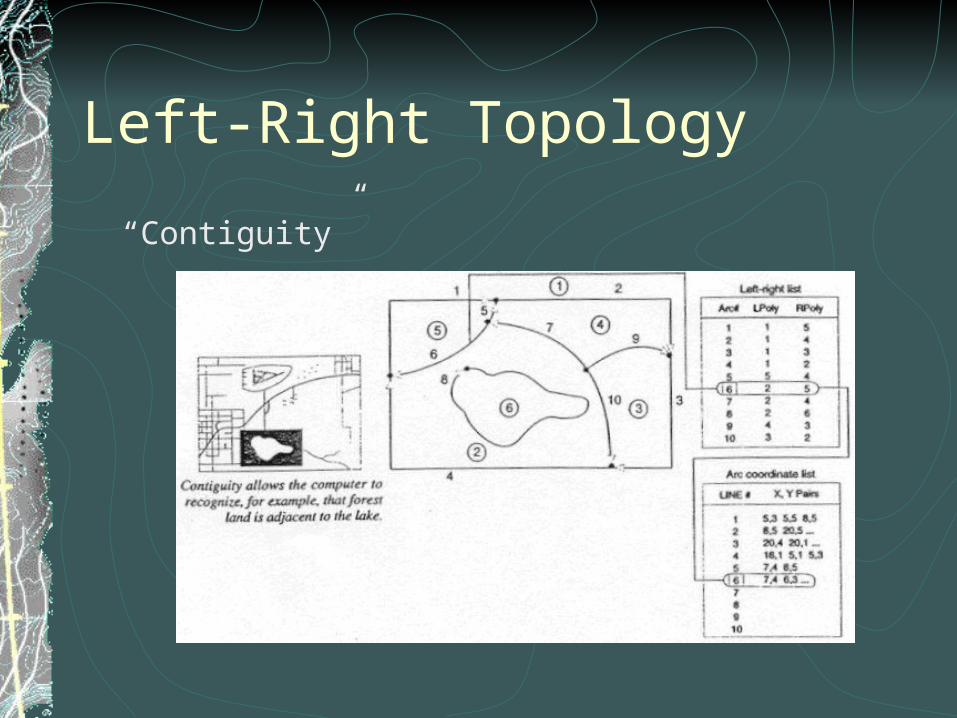
Left-Right Topology

“Contiguity”

Map FeaturesMap features are organized into a set of layers or “themes”Base maps are organized into "layers"

CoverageEach layer in GIS is termed a "coverage“ – consisting of topologically linked geographic features and associated data

Soils Attributes

ID Soil Class Suitability

1 A3 113 HIGH

2 C6 95 LOW

3 B7 212 MODERATE

4 B13 201 MODERATE

5 Z22 66 LOW

6 A6 77 HIGH

7 A1 117 LOW

Features and RepresentationsFeature Class Application and Use Examples

Arcs Linear features Streets, contours, streams, sewers, power lines, gas lines

Nodes Points along linear features Valves on pipelines, intersections on streets, power poles, manhole covers

Label Points Point locations Well sites, mountain peaks

Polygons Area features Soil units, land use, parcels, building footprints, forest stands, ownership

Tics Geographic registration and control Registration for digitizing

Annotation Feature labels Street names, place names on road maps

Links Rubber sheeting and adjustment Edge-matching map sheets, feature snapping, datum adjustments

Routes Linear features Streets, contours, streams, sewers, power lines, gas lines, and street addresses

Sections Define route features --

Coverage Extent Defines map extent --

Storing AttributesGIS databases store descriptive attributes associated with map features similarly to the way it stores coordinates

Feature Attribute Table

Roads Map

Connecting Features and AttributesThere is a one-to-one relationship between map features and records in the feature attribute tableThe link between the feature and the table is maintained through a unique numerical identifier assigned to each feature (i.e. points, arcs and polygons)This unique identifier is stored in two places; the file that contains the x-y coordinate pairs, and the corresponding record in the feature attribute table

FEATURE NO. X,Y PAIRS

1 3,5 5,5

2 5,5 8,5

3 8,5 11,5

4 6,9 5,8 5,7 5,6 5,5

5 5,5 4,4 4,1

6 8,5 8,7

Unique Identifier

Attribute Table

Feature Coordinates

Joining TablesAny two attributes tables can be joined if they share common attributes -- using "relate" and "join" operators

Joined Attribute Table

SummaryAll GIS data is stored as a point, spline or polygon!Attributes can be attached to any of these geographic entities!The power of GIS comes from the ability to relate and manipulate attribute databases along with the geographic entities!When using GIS, one must observe and practice safe data!

Map Projections

Mathematical operation in which Cartesian coordinates (x,y) are written as parametric functions of latitude () and longitude ().

x = fx( y = fy(

Allows longitude and latitude coordinates to be projected from 3-D position on the earth’s surface onto a 2-D plane.Several projections exist to preserve different aspects (e.g. angles, distances, areas).

Classes of Map ProjectionsConformal (orthomorphic) – angles between short intersecting lines are preservedEqual-Area – area is preserved, angles are distortedEquidistant – distances are properly representedAzimuthal – direction of any point with respect to a central point is preserved

Basic Types of Map ProjectionsGnomonic – used for navigational purposesStereographic – excellent projection for general maps showing a hemisphereOrthographic – appears as a photo taken from deep spaceConical – sufficiently accurate for maps of considerable areas (used by the USGS and USNOS)

Gnomonic Projection

Stereographic Projection

Orthographic Projection

Conical Projection

(a) cone tangent to a sphere, (b) cone tangent to a sphere with standard tangent closer to the equator, (c) cylinder tangent to a sphere at the equator, (d) cone with standard parallel at higher altitudes, and (e) plane tangent to a sphere at the pole.

Polyconic ProjectionsPoints on the earth’s surface projected onto a series of frustums (sections of cones)Used when performing conformal mapping

Polyconic Projections

Conformal (Orthomorphic) Mapping

Projection that preserves the angle between short , intersecting line segmentsAKA “orthomorphic”A direct relationship between map coordinates (x,y) and geodetic coordinates () does NOT exist

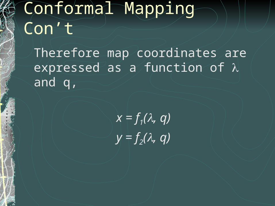
Conformal Mapping Con’tTherefore map coordinates are expressed as a function of and q,

x = f1(, q)

y = f2(, q)

Lambert Conformal Conic ProjectionMost widely used projectionBasis of State Plane coordinate system – used in states with a greater East-West than North-South distancesConic projection with two standard parallels

Lambert Conformal Conic Projection

Lambert Conformal Projection

3-D3-D 2-D2-DProjectionProjection

Map projection on a cylinder tangent to the earth’s equatorCoordinates x and y are represented by:

x= y = q

where = longitude and q = isometric latitudeMeridians are equally spaced vertical lines, parallels are unequally spaced horizontal linesValuable for navigation – used by U.S. Military

Mercator Projection

Mercator Projection

Cylinder for earth area to be projected onto.

Uses the Orthographic projection

Note:

Transverse Mercator Projection

Horizontal Datums

Mathematical model that depicts the shape and size of the earth (earth’s mean, sea-level surface)Earth is described as a “oblate ellipsoid” of revolution, or as an “oblate spheroid” – not a perfect sphereNecessary to determine the position of GPS satellites orbiting the earth, and ultimately, the location of a GPS receiver

Common Datums

NAD 27 - North American Datum of 1927, based on the Clarke Spheroid of 1866NAD 83 - North American Datum of 1983, based on the GRS 80 derived ellipsoidWGS 84 - World Geodetic System, developed by the US Military in 1984 (basis of GPS receiver calculations)

Ellipsoid Models

Name

Year

Equitorial Radius

(m)

Polar Radius

(m)

Clarke

1866

6,378,206

6,356,584

GRS 80 1980 6,378,137 6,356,752

Universal Transverse Mercator (UTM)

A coordinate system based on the transverse mercator projectionUTM - projection in zones of 6°Reference ellipsoid -- Clarke 1866 for North America.Origin of longitude -- central meridian (CM)Origin of latitude -- equatorUnit of measure -- meter

Universal Transverse Mercator (UTM)Con’t

False Northing - 10,000,000 m is used in the Southern hemisphereFalse Easting - 500,000 m is used for the central meridian of each zoneThe scale factor at the central meridian is 0.9996Zones are numbered with 1 beginning at 180° and 174° W meridians, and increasing to 60 for the zone between 174° and 180° E meridiansLatitude for this system varies between 80°N and 80°S

State Plane Coordinate System (SPCS)

Projects raw GPS data (lat/lon) into a coordinate system to perform dimensional analysisWidely used coordinate system within the U.S.Used by many PA and GIS packagesLambert Conformal Conic and Transverse Mercator are used as the basis of the State Plane Coordinate System

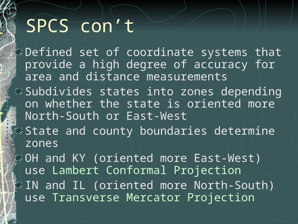
SPCS con’tDefined set of coordinate systems that provide a high degree of accuracy for area and distance measurementsSubdivides states into zones depending on whether the state is oriented more North-South or East-WestState and county boundaries determine zonesOH and KY (oriented more East-West) use Lambert Conformal ProjectionIN and IL (oriented more North-South) use Transverse Mercator Projection

Easting and NorthingEach zone has an origin which is located west and south of the zone so that the x and y coordinates are positive A false Easting value is often added to the x-coordinateSimilarly, a false Northing is added to the y- coordinate.Positive x and y directions are referred to as ‘Easting’ and ‘Northing’ directions

Kentucky North State Plane Coordinates (NAD 83)

Standard Parallels37o58’ N to 38o58’N

Origin84o15’ W, 37o30’ N

False Easting and Northingx=500,000 ft and y=0 ft

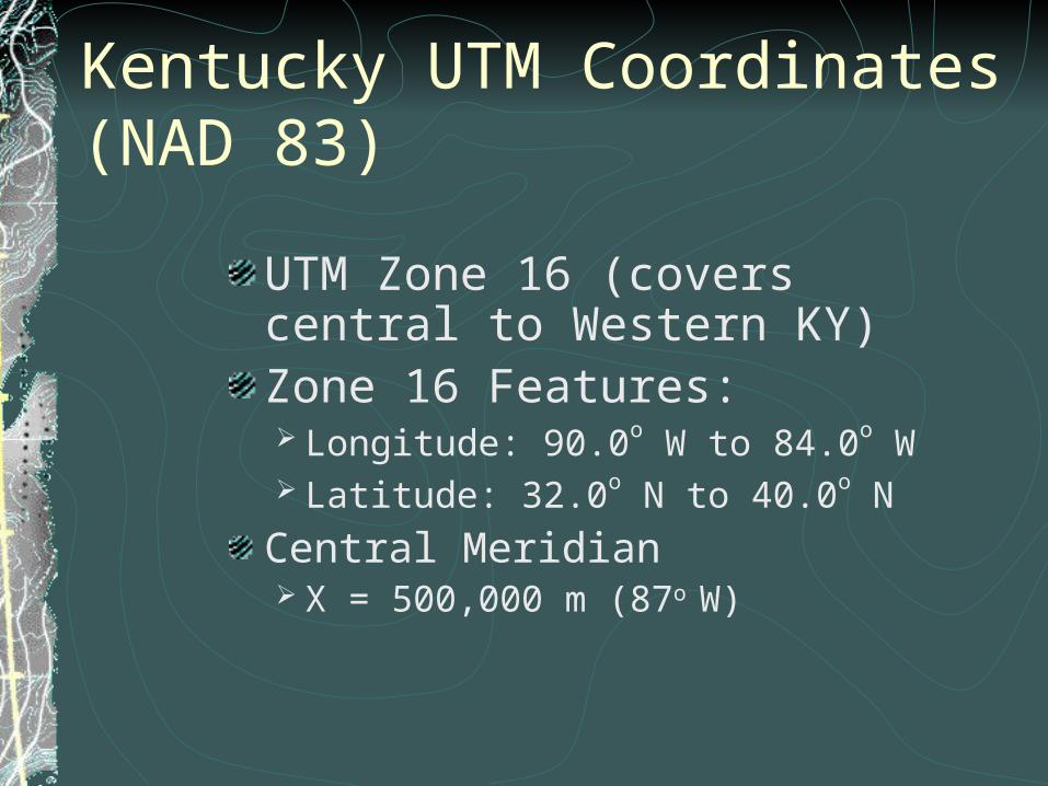
Kentucky UTM Coordinates (NAD 83)

UTM Zone 16 (covers central to Western KY)Zone 16 Features: Longitude: 90.0o W to 84.0o W Latitude: 32.0o N to 40.0o N

Central Meridian X = 500,000 m (87o W)

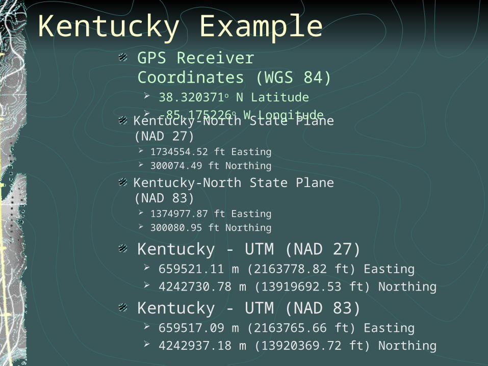
Kentucky Example

Kentucky-North State Plane (NAD 27) 1734554.52 ft Easting 300074.49 ft Northing

Kentucky-North State Plane (NAD 83) 1374977.87 ft Easting 300080.95 ft Northing

GPS Receiver Coordinates (WGS 84) 38.320371o N Latitude -85.175226o W Longitude

Kentucky - UTM (NAD 27) 659521.11 m (2163778.82 ft) Easting 4242730.78 m (13919692.53 ft) Northing

Kentucky - UTM (NAD 83) 659517.09 m (2163765.66 ft) Easting 4242937.18 m (13920369.72 ft) Northing

SummaryGNSS use the WGS 84 datum!NAD 27 and NAD 83 datums produce different x-y coordinates for UTM and SPCS!SPCS and UTM provide the ability to perform dimensional analyses!One must know (and specify) the datum, projection and units when adding data to a GIS database!