research collection28704/... · derivation of a 1-d thermal model of vehicle underhood temperatures...
TRANSCRIPT

Research Collection
Master Thesis
Derivation of a 1-D thermal model of vehicle underhoodtemperatures on the basis of test data using an evolutionaryalgorithm
Author(s): Apolloni, Marco
Publication Date: 2006
Permanent Link: https://doi.org/10.3929/ethz-a-005189116
Rights / License: In Copyright - Non-Commercial Use Permitted
This page was generated automatically upon download from the ETH Zurich Research Collection. For moreinformation please consult the Terms of use.
ETH Library

Diploma Thesis 1 17.02.2006
Derivation of a 1-D Thermal Model
of Vehicle Underhood Temperatures on the Basis of Test Data Using an
Evolutionary Algorithm
Diploma Thesis WS2005/2006
Marco Apolloni
ETH – Swiss Federal Institute of Technology
Department of Mechanical Engineering
Rieter Automotive Management AG
Supervision: Hermann de Ciutiis
Prof. Dr. Aldo Steinfeld

Diploma Thesis 2 17.02.2006
Table of content
Table of content ....................................................................................................................2 A. Introduction...............................................................................................................4
1. PREFACE.......................................................................................................................... 4
2. ABSTRACT........................................................................................................................ 4
3. INTRODUCTION ............................................................................................................... 5
4. LITERATURE RESEARCH ................................................................................................... 6 B. Analysis of on-road measurements ......................................................................... 10
1. INTRODUCTION ............................................................................................................. 10
2. CONSIDERATIONS OF THE SYSTEM................................................................................. 10
3. MEASUREMENT CONDITIONS......................................................................................... 11
4. TEMPERATURE ANALYSIS ............................................................................................... 12
4.1. Temperature analysis of Renault Mégane........................................................................ 12
4.1.1. Body temperatures......................................................................................... 13
4.1.2. Heatshield temperatures ................................................................................ 13
4.1.3. Air temperatures above and under the heatshield........................................... 14
4.1.4. Exhaust temperatures .................................................................................... 14
4.2. Temperature analysis of Nissan Skyline......................................................................... 15
4.3. Influence of changing grade and velocity........................................................................... 15
4.4. Formulation of rollerbench testing procedure..................................................................... 17 C. Experimental data acquisition ................................................................................ 18
1. INTRODUCTION ............................................................................................................. 18
2. ON-ROAD VERSUS ROLLERBENCH MEASUREMENTS ........................................................ 20
3. MEASUREMENTS ............................................................................................................ 20
3.1. Introduction .............................................................................................................. 20
3.2. Repeatability............................................................................................................. 21
3.3. Problems .................................................................................................................. 24
3.3.1. Temperature drift – Control of ambient air temperature................................ 24
3.3.2. Velocity measurements – Pulse-to-DC converter........................................... 26
3.4. Underhood measurements ............................................................................................ 26
3.4.1. Cooling circuit – Fan activity ......................................................................... 26
3.4.2. Tunnel entrance inlet temperatures................................................................ 27
3.4.3. Average gas manifold temperature................................................................. 28
3.4.4. Radiator effectiveness .................................................................................... 29
3.4.5. Thermostat behavior at the heat-up phase ..................................................... 30
3.5. Underbody measurements ............................................................................................ 30 D. Derivation of a 1-D thermal model..........................................................................33
1. INTRODUCTION ............................................................................................................. 33
2. 1-D TRANSIENT UNDERHOOD MODELING ..................................................................... 33
2.1. Matlab model ........................................................................................................... 34
2.2. Simulink/Matlab-model............................................................................................. 38
2.2.1. Motor-vehicle dynamics – Engine calculation ................................................ 39
2.2.2. Thermostat purpose and modeling ................................................................ 42
2.2.3. Fan modeling................................................................................................. 43
2.2.4. Thermodynamic balance................................................................................ 45
2.2.5. Thermodynamic equations ............................................................................ 45
2.2.6. Implementation of Simulink/Matlab ............................................................. 50
2.2.7. Data input – Signal builder ............................................................................ 50

Diploma Thesis 3 17.02.2006
2.2.8. Simulink solver .............................................................................................. 51
2.3. First evaluation of the Simulink model .......................................................................... 52
2.4. Evolutionary Algorithm.............................................................................................. 53
2.4.1. Introduction .................................................................................................. 53
2.4.2. Application for 1-D Simulink/Matlab-model................................................. 55
2.4.3. Structure of the calculation process ............................................................... 57
2.4.4. Objective value.............................................................................................. 58
2.5. Improvements of the Simulink model ............................................................................. 59
2.5.1. Measurement with repositioned thermocouples............................................. 59
2.5.2. Sensitivity analysis.......................................................................................... 59
2.5.3. Change of the model ..................................................................................... 60
2.5.4. Comparison: Model and measurement........................................................... 62
2.5.5. Investigation on different parts of the test ..................................................... 66
2.5.6. Dissipated heat to coolant and exhaust gas .................................................... 67
2.5.7. Local nucleate boiling at the cylinder head wall.............................................. 68
2.5.8. Investigation on a set of guessing parameters ................................................ 70
2.5.9. Engine compartment heat-up explanation ..................................................... 71 E. Conclusion...............................................................................................................72 F. Outlook....................................................................................................................73 G. Appendix .................................................................................................................74
10. HEAT CAPACITY CALCULATION OF EXHAUST AIR ....................................................... 74
11. MEASURED ON-ROAD TEMPERATURES FOR THE UNDERBODY REGION ...................... 75
12. MATLAB-MODEL ........................................................................................................ 81
13. SIMULINK/MATLAB-MODEL ...................................................................................... 88
14. MEASUREMENT PROTOCOLS ...................................................................................... 97
15. MEASUREMENT POSITIONS ...................................................................................... 104
16. NOMENCLATURE AND ABBREVIATIONS................................................................... 108
17. LIST OF FIGURES AND TABLES .................................................................................. 110 H. References ..............................................................................................................112 I. Acknowledgements ................................................................................................114

Diploma Thesis 4 17.02.2006
A. Introduction
1. Preface
This Diploma Thesis was done at Rieter Automotive Management AG in Winterthur, Switzerland. Rieter Automotive is one of the world's leading suppliers of noise control and thermal insulation systems in motor vehicles. Their systems, developed in close co-operation with the major vehicle manufactures, integrate noise reduction and thermal management optimization. This work was elaborated in the Thermal Management Division, one of the many so-called Centers of Excellence (CoE). It was supported by Mr. Hermann de Ciutiis, Head of CoE Thermal Management as well as by Dr. Aldo Steinfeld, Professor at the Department of Mechanical and Process Engineering at the Swiss Federal Institute of Technology in Zurich (ETHZ).
2. Abstract
The influence of environmental changes on underhood and underbody components of a vehicle during various driving cycles is an important issue in the automotive industry. Several approaches for the simulation of cooling system temperatures in the underhood region have already been made in the past. 1-D modeling for automotive cooling systems is a common procedure for manufacturer to improve different components of a vehicle. Generally, these simulations are based on detailed data of each component measured on a test bench. Beside mass flow measurements, pressure distributions and heat fluxes are measured and fed into a simulation program as boundary condition for component improvements. For more detailed information, 1-D models are coupled with 2-D and 3-D simulations to get more reliable results. From the view of a supplier, most of these data are not available and detailed measurements of different components are too cost intensive. Furthermore, investigations have to be done on many different vehicles with completely different arrangements. Nevertheless, influences of changing environmental and driving parameters are important to investigate temperature distributions at different positions of a vehicle. For that reason, it has been determined if important vehicle underhood and underbody temperatures can be predicted with a new approach. A derivation of a 1-D thermal model on the basis of test data using an evolutionary algorithm is introduced. The simulation incorporates any given information from technical data sheets of the investigated vehicle. Further parameters that can be measured easily are included as well for a proper calculation. In addition, a set of guessing parameters is defined to describe the system as a whole. These guessing parameters are physically meaningful because they characterize a specific relation in the heat transfer calculation for the one-dimensional model. The simulation is then conducted and fed with the measured data to find appropriate values for the set of guessing parameters within a given range. For that purpose, an evolutionary algorithm is used leading to a fast determination of the unknown coefficients. Using the resulting parameters, influences of changing environmental and driving conditions can then be investigated.

Diploma Thesis 5 17.02.2006
3. Introduction
Thermal management is a key part in the heat protection and design optimization of state of the art vehicles. It unifies thermal and aerodynamic engineering aspects and it is often coupled with acoustic considerations. For the improvement of vehicle performance, test facilities play a very important role as well as various simulation tools (e.g. Computer Aided Engineering: CAE). Beside the measurement tests on the test rig and the simulation procedure, on-road tests are important to simulate real life driving cycles where all of the engineering parameters are dependent of environmental conditions, topography of the road-test route as well as driver operation characteristics. When such on-road tests are performed, it gets difficult to properly understand the behavior of vehicle temperature changes due to many influencing parameters. A problem is the fact that in general, road measurements are difficult to reproduce. Nevertheless, it is very important for an engineer to compare on-road tests with data acquired from the test bench as well as from numerical simulations. Before this comparison can be drawn, influences of single changing parameters have to be understood, which can be simulated in the controlled rollerbench environment. At Rieter Automotive Management AG, different driving cycles have been evaluated. Two of the important ones are the high-speed test cycle as well as the hill-climb test cycle. With these measurement tests, the different thermal limits of the vehicle are investigated. Thermal safety has to be guaranteed; simulation is a supporting tool securing thermal protection. The influence of changing ambient temperatures on underhood and underbody components is of strong interest. Until now, a simple normalization to 20°C ambient temperature was applied using the online ambient temperature for the comparison of the temperatures of components measured on different tests. The ambient air temperatures have furthermore been averaged in order to reduce noise due to strongly oscillating ambient air temperatures. The normalization was defined as follows:
CTTT ambientmeasurednew °+−= 20
where Tnew is the wanted normalized temperature at 20°C, Tmeasured the measured component temperature and Tambient the measured ambient air temperature. This rough normalization has been in good agreement with some measurement points on the vehicle. Unfortunately, most of the measurement points have showed that this formula is not applicable at all. The reason for that is that the aerodynamics around a vehicle is very complex due to the underhood and underbody geometry, changing on-road conditions and varying heat transfer mechanisms at each measured position at the vehicle. Furthermore, the cooling system behavior influences the temperatures in the underhood and underbody region due to electric fan activation. This implies a detailed investigation of the ambient impact on vehicle temperatures.

Diploma Thesis 6 17.02.2006
4. Literature research
Thermal management is a key research issue for vehicle performance improvement. Beside vehicle testing, simulation tools become more and more important regarding the shortened development cycle of a vehicle. There are several different approaches for thermal investigations; most of them include a combination of simulation and testing. Even if aerodynamic and thermal simulations become more and more important, measurements for validations are inevitable. Literature research shows the importance of the thermal investigations either for safety and comfort as well as for the overall-performance of a vehicle. Depending on the Original Equipment Manufacturer (OEM), standard temperature limit at the underbody is set at approximately 80°C. This limit ensures that carpets and other trim materials or sensitive components are not damaged by heat, [I]. The thermal protection in the underbody region close to the exhaust line tunnel is therefore very important. Different heatshields are developed to reduce infrared radiation from the exhaust line and attenuate heat transfer. They are mounted very close to the underbody with a small open gap allowing hot engine air to flow above the heatshield. All underbody optimizations are done with the goal to reduce thermal transfer to the cabin while keeping the drag coefficient of the vehicle low. Additional closing of the tunnels with covers have also been investigated to reduce the aerodynamic drag. The cost intensive vehicle testing has pushed on the integration of CAE tools in recent years. While major improvements in CAE in some areas have had a significant effect toward this goal in areas such as crash testing, the prediction of vehicle temperatures remains a largely test-driven process. Engine cooling may be relatively accurately computed, but calculation of the temperatures on the vehicle body and components and hence the need for heat shielding is usually not, [II]. Furthermore, a very detailed and accurate 3-D modeling is often done only for steady-state analysis because computing hardware available being too limited for a transient analysis of this scale. Heat transfer coefficient calculations are often based on Nusselt-correlation in literature for simplified geometries. One problem remains in the calculations that aerodynamic models with the use of Computational Fluid Dynamics (CFD) have to be coupled with thermal models in an iterative way. The underbody region cannot be considered alone, because it is strongly dependent on the temperatures and flow parameters upstreams. That means that it is inevitable to understand in a proper way how parameters in the underhood region (e.g. fan exit air temperatures, engine surface temperatures and ambient air mass flow) react before starting with the calculation of underbody parameters. Considering the heat transfer rate at any location, the following transient formula has to be applied:
( ) ( ) ( )
p
fnS
cm
TThx
kTTATT
t
T
⋅
−⋅+∆
⋅−+⋅⋅⋅⋅−=
∂
∂ 21
44εεσ
Especially for the application of the underbody region, all heat transfer modes are very important. Radiation from the exhaust line, forced convection induced by vehicle speed and/or fan air flow (and natural convection while stopping) and lateral conduction in the aluminum heatshield are crucial beside many more thermal interactions in the lower region of a vehicle. Prediction of idealized, steady-state temperatures at full vehicle level in this way yields to a low return of information for effort expended. An alternative method involving the use of a single

Diploma Thesis 7 17.02.2006
CFD analysis, to generate a 1-D flow network for use in the thermal models is currently being applied to vehicle models. This also allows the possibility of transient computation that is of considerably higher value for temperature predictions on parts such as carpets, which never reach the idealized steady-state temperature, [II]. Underhood and underbody simulation for development of new vehicles is a big research topic. In [III], [IV], [V], [VI], [VII] and [VIII], the recent developments regarding the thermal investigation with simulation tools are discussed. Most of them show the coupling of temperature and flow field where some of them only discuss the steady-state approach. In [VII] it is shown that transient computations including free convection and thermal radiation becomes feasible. When focusing on Underhood Thermal Management (UTM) the application of CFD provides in the early concept phase valuable information about component temperatures to be expected and the distribution of flow mass under various driving conditions. Furthermore, sensitivity analysis has been performed concerning different parameters in the model. In most of the investigations, it has been focused on high-speed vehicle simulation as well as on hill-climbing drives of cars pulling heavy load trailers that are to be classified more critically. Due to low air velocities passing through the engine compartment, convective heat transport is reduced so that extreme surface temperatures are to be expected. Additionally, during the consecutive cool down phase components are subjected to maximum thermal loads, when located in the proximity of hot exhaust pipes. Currently the numerical simulation cannot entirely replace experimental analysis, however, it provides additional valuable information about spatial structures of temperature and velocity fields. Applying model-modularization and a combined experimental/numerical practice, complex transient physical phenomena can be simulated. In this fashion, the application of CFD, as it is an efficient analysis tool, supports the experimental investigation of underhood and underbody vehicle flow to further enhance efficiency in the vehicle design process, [VII]. In the automotive industry, the simulation tools are divided in three main categories, [VIII]:
• 1-D cooling system analysis
• 1-D engine modeling
• 3-D fluid flow and heat transfer analysis
The use of 1-D cooling system analysis tools is standard in the development of cooling systems in the concept phase. In order to predict accurately the performance of a cooling module located within the underbonnet, it is desirable to have the installed mass flow rate of air onto each heat exchanger and the heat rejection to the coolant and oil from the engine. Engine modeling tools in 1-D have gained significant acceptance within the power train development community. Temperatures of the engine components can be calculated along with the heat transfer to the oil and coolant. Exhaust gas temperatures, fuel consumption and engine performance can all be calculated as long as detailed information of all components is available. This data can be valuable data for 1-D cooling system models and these tools have frequently been used together to enhance thermal management system development. Complex 3-D CFD models have been used for around a decade to investigate the isothermal airflow structure around the vehicle including the underbonnet. Heat transfer calculations in 3-D are less common and have mainly been limited to convection with radiation calculated independently using specialized radiation packages. Table A-1 shows the data required and the data calculated for other UTM tools:

Diploma Thesis 8 17.02.2006
Simulation Tool
Data required Data calculated
1-D cooling system analysis
- Component performance data - Engine heat rejection data to
coolant and oil - Geometric details of system layout
- Installed mass flow rate of air to cooling pack
- Heat rejection from fluids to underbonnet domain
- Coolant and oil temperatures
1-D engine modeling
- Geometric details of engine design
- Empirical data for calibration
- EMS control strategy
- Heat rejection to the fluids
- Exhaust and induction surface temperatures
- Exhaust and induction mass flow rates
- Energy released from the combustion process to fluids, friction, exhaust, shaft power etc.
3-D fluid flow and heat transfer
- Geometric representation of full vehicle including all components to be included in the analysis
- Meshed computational domain
- Performance data for heat exchangers and fan(s)
- Material properties of solids
- Intake and exhaust mass flow rates
- Heat transfer coefficients
- Installed mass flow rates onto the heat exchangers
Table A-1: Data of simulation tools, [VIII]
The results of the different models are given in [VIII] and show good correlation for several parameters like torque, airflow and exhaust gas temperatures. The latter were important for predicting realistic exhaust system wall temperatures, which are fundamental for the correct temperature distribution in the underbody region. The work has shown that linking software tools together can give accurate predictions of the coolant and oil temperatures. In [IX], different approaches for providing appropriate thermal protection in the underbody region are discussed. The skin temperature of various components of the exhaust system such as manifolds, catalytic converter, connecting pipes, muffler etc. are predicted. It has been shown that exhaust system results in high temperatures that may be above the permissible material and/or operational limits of the component. This makes it essential to monitor the temperatures of all components that may be at risk of failure due to thermal loads and provide appropriate thermal protection. This could be achieved by:
• Relocating the component
• Insertion of heatshields between the exhaust and the component
• Innovative airflow management techniques that increase the convection around the component
Another important benefit of performing simulations is that, when physical tests are being carried out, the locations for placement of thermocouples are based on the thermal map obtained from the simulation.

Diploma Thesis 9 17.02.2006
It is not the goal of this Diploma Thesis to work out a simulation based on CAE programs like STAR-CD, FLUENT or RadTherm. Still, it is important for the upcoming investigation to find out what has been already done and to include several cognizances from previous research. As it can be seen in this literature research chapter, there are many different approaches for solving thermal problems in the underhood and underbody region. Most of them are based on any kind of simulation with or without additional coupling. Nevertheless, the influence of changing ambient air temperatures, initial conditions or environmental changes for a latter comparison has not been discussed so far. Furthermore, a lot of important parameters in the whole vehicle system (e.g. cooling circuit) are not known and/or are very time-intensive to measure. Detailed information about different components of the vehicles is not available from the OEM’s. Here arises the idea of introducing different guessing parameters that are not known, but are constant over the measurement cycle. With the right physical behavior of the heat transfer interactions, a 1-D dynamic system can be built up and afterwards fed with measurement data from the vehicle. For determining the unknown coefficients, an evolutionary algorithm is used. This approach to build up a simplified 1-D dynamic model and feed it with real data using an evolutionary algorithm is new. The original equipment manufacturers generally take into account many more parameters for the optimization of each component. For the understanding of the system behavior, though, this approach leads to the dependencies of all node temperatures and will show the sensitivities of the different input parameters. To use the 1-D simulation method based on network theory, a high degree of abstraction will be necessary regarding the vehicle as a very complex system. It will also give the answer if it is even possible to predict important vehicle temperatures with the help of a 1-D model without knowing detailed geometry and mass flow information. A transfer of the model with modifications to different vehicle types (e.g. diesel or gasoline engines, including or excluding turbocharger and/or intercooler) can then be discussed. The use of evolutionary algorithms in general, on the other hand, is not new in the automotive research branch. However, it is mainly used for the optimization of individual components. Vehicle thermal system optimization using genetic optimization algorithms was investigated in [XIV]. It has been shown that the general nature of the evolutionary algorithm is very beneficial in searching for optima in complex systems where the range of the variable space is huge. Beside optimization problems discussed also in [XV], an important field of application is the vehicle navigation system where evolutionary algorithms are used to search the best route in the shortest possible time, [XVI].

Diploma Thesis 10 17.02.2006
B. Analysis of on-road measurements
1. Introduction
Prior to my work at Rieter Automotive for the upcoming project, several on-road measurements have been done. The investigated cars were the Renault Mégane 1.5l dCi and the Nissan Skyline 2.5l V6. Even though the aims of these studies did not concern a temperature model for vehicle measurements, the data can be used for a first temperature analysis. The influences of ambient air temperature and other changing parameters during the on-road tests are not well understood, yet. On the other hand, tests on the test facility with a very good controlled environment can give very accurate information about various investigations already done at Rieter Automotive. The influence of ambient air temperature change has never been tested on the rollerbench because the goal of these measurements used to be the elimination of additional influences of the test cycle. A test series has shown that the mean temperature difference in ambient air can be held below 2°C. Due to this small difference the influence of changing ambient air was neglected completely. When the transition is done to on-road tests, this is not valid any more. Ambient air is changing rapidly due to changing environmental conditions. For example, weather conditions and altitude (standard hill-climb test goes from 400 to 1600 meters above see level) will have a strong impact on ambient air temperatures. Atmospheric inversion and hindrances during the drive (e.g. tunnel section within the test cycle) have an additional impact on the ambient air characteristics. The question oft the influence of changing ambient air temperatures from the customer-side is therefore justifiable and has to be investigated.
2. Considerations of the system
Before the analysis of the available data is done, a closer look at the system is necessary to find out which parameters can influence the measurement tests. Figure B-1 shows some of the most important factors that have a direct impact on the test results.
Figure B-1: Transfer function for measurement tests
The so-called transfer function describes the input/output behavior of the system. The system itself is influenced by several changing parameters. Most of them are negligible for the

Diploma Thesis 11 17.02.2006
rollerbench tests due to a controlled environment. For the on-road tests, many parameters cannot be neglected anymore. The main contributors are the changing ambient air temperature, the various initial conditions and the strong influence of the driving cycle. It is important to keep the interacting parameters in mind because on-road tests are real life cycles where no ideal conditions do exist.
3. Measurement conditions
Beside several possible driving conditions, it has been focused on hill-climb tests. These tests are important for passenger comfort and safety regarding the peak temperatures of different components that can be obtained. It is crucial that all temperatures stay within a given range and that the critical temperatures are not transgressed during the whole driving cycle. The on-road tests have been done on the route between Triesen and Malbun (FL). The main reason for choosing this test section is the grade distribution over the test route of 12 km with an average incline of 9.6%. The slope can be seen in Figure B-2.
Figure B-2: Profile of hill-climb test from Triesen to Malbun (FL)
The main disadvantage is the existence of three traffic lights in between the test section. So for the different cycles, various waiting times were obtained because it was not possible to shut down this street for the measurements. The testing procedure was held the same for all measurements:
I: Driving from Winterthur to Triesen: Driving time between 60 and 80 minutes.
II: Constant heat-up phase with 80 kph on the highway in the 5th gear for 7 minutes. III: Driving to the test start for 4 minutes. IV: Test start with 25 kph in the 1st gear for the whole hill-climb test (driving time 27 minutes). V: Test stop at the top of the hill in Malbun. VI: Soak or idling phase at the top before returning to Triesen. VII: Cool-down of the vehicle before the next start.
Because of the extent of the test procedure, only three tests could be done in one day. To minimize the influence of the traffic lights, 3500 rpm are held in idling during the waiting time. Measurements have shown that these waiting times are critical and make a direct comparison between different tests very difficult. The forced convection in the underbody region is completely stopped during the halt (except for occurring wind speeds, which are not measured on the vehicle) and the natural convection is getting predominant. Depending on the geometry of the underbody and its covering, the influence can be too strong to make a later comparison with other measurements impossible.

Diploma Thesis 12 17.02.2006
4. Temperature analysis
The analysis of different on-road measurements have shown that exact information about component temperature behavior in dependency of ambient air temperatures alone cannot be given due to additional changing parameters during the on-road tests like the numerated in Figure B-1. Some of them might be negligible (e.g. humidity) because their impacts are very small. Measurements on rainy days have been avoided completely. On the other hand, initial conditions, driving cycle and weather conditions have a direct influence on the measured temperatures. With the initial condition, the different starting condition after the warm-up phase is meant. Regarding the driving cycle, all the influences from the driver as well as road conditions have to be taken into account. These are the non-uniform vehicle speed, the different incline of the road, and especially the three traffic lights on the test route. Nevertheless, a first broad forecast can be given while looking at the corrected data (driving time and traffic light waiting time). With this quantitative information, meaningful procedures have to be formulated for testing the influences of these parameters on the rollerbench separately. In the test facility, a controlled environment is available so most of the additional dependencies can be cut out that would always be present in real driving cycles. The first goal is to find a way to correlate measurements on the rollerbench with different conditions (e.g. changing ambient air). Only if these influences are well understood, the transition can be done to correlate data from the rollerbench with the real on-road test data.
4.1. Temperature analysis of Renault Mégane
For the analysis of the Mégane measurements, all data have been prepared and scaled to compare the different measurements with each other. The waiting time has been cut out as well as the warm-up and soak phase. The temperature versus time charts became temperature versus distance charts where each test could be compared with each other. The measurement sensors (thermocouples K-type) were placed in the underfloor tunnel in four sections, measuring from the bottom to the top:
• Exhaust line surface
• Air between exhaust line and heatshield
• Heatshield
• Air between heatshield and body
• Body
Figure B-3 shows the locations of the thermocouples.
Figure B-3: Location of the temperature measurement in the underbody part

Diploma Thesis 13 17.02.2006
4.1.1. Body temperatures
[°C] tunnel 1 tunnel 2 tunnel 3 tunnel 4 amb start
temp. end temp.
start temp.
end temp.
start temp.
end temp.
start temp.
end temp.
base 1 47.9 81.2 45.2 65.4 41.4 57.6 34.3 40.6 21.5 base 2 50.4 81.5 44.2 64.8 42.4 58.6 34.4 40.8 20.8 base 3 63.4 86.8 51.1 71.5 48.9 66.1 39.4 48.2 26.7
Table B-1: Starting and ending temperatures at body position for all sections
Figure G-1, Figure G-2 and Figure G-3 in the appendix show that the two different
measurements with almost the same ambient temperatures (∆Tmean=0.7°C) are in good correlation. Even if the starting temperatures are slightly different, they are converging with time. Starting conditions should therefore be negligible for the stationary state as long as the ambient temperature is constant. That means that the stationary body temperature is insensitive to small staring condition variations. On the other hand, the absolute value of the ambient temperature will influence the temperature of the body considerably. A mean temperature difference of approximately 5°C in ambient temperature will result in a mean temperature difference between 4.9°C and 9.3°C, depending on the section of measurement.
tunnel 1 tunnel 2 tunnel 3 tunnel 4 mean standard deviation σ
3.08 0.94 1.32 0.86
in % of mean 53.84 13.53 15.82 12.78
Table B-2: Mean standard deviation of the temperature offsets
Table B-2 shows that the variations of the temperature offsets are in the range of 13 – 16% for the last three sections. In section one, the deviation is very big due to a converging characteristic of the measurements. The reason for that cannot be given by a simple calculation. It has to be tested on the rollerbench as well as in the simulation if this behavior can be approved. The fluctuations of the body temperatures in general are very small due to the inertness of the body itself that is shielded from the exhaust line with an aluminum heatshield. The data has to be validated on the rollerbench test especially to see how the body temperature differences are going to change for different ambient air temperatures. Still, it seems that for all tunnel measurement positions 1-4 the dependencies stay the same due to the simple tunnel geometry that is equal for all sections of the underbody (no additional components which can have a strong influence on the sections downstream due to secondary air flow mixing phenomena). Beside the ambient air temperature change, it is important to do at least one test with a very long time period. The reason for that is to find out the time response of the different components. In general, the hill-climb test takes about half an hour. In this time, even with the preconditioning, a steady-state condition is not obtained for most of the components. Even if it seems that temperatures are stable, they are still in the transient phase and increasing slowly. The transient behavior is therefore very important for the investigation.
4.1.2. Heatshield temperatures
The temperature characteristics for the heatshields are very hard to predict. First, the fluctuations in general are very high. The difference of driving cycle, for example, will directly influence the heatshields. The time response for the first heatshield position is around 10 minutes and fast

Diploma Thesis 14 17.02.2006
compared to the body position. At heatshield position 1, 3 and 4, the initial conditions differ only slightly, whereat position 2, the initial temperatures for the approximately same ambient temperature differ by 10°C. The bottom line is that for heatshield temperature comparison, all possible noise has to be eliminated before any prediction and correlation can be done.
4.1.3. Air temperatures above and under the heatshield
The air above and under the heatshield has been measured as well during the test cycle. The positions have been chosen in half of the distance between exhaust and heatshield and between heatshield and body, respectively.
∆Tbody-heatshield tunnel 1 tunnel 2 tunnel 3 tunnel 4
baseline 1 10.7°C 5.1°C 3.5°C 3.9°C baseline 2 8.7°C 7.6°C 0.6°C 2.3°C baseline 3 11.5°C 9.2°C 4.7°C 1.7°C
∆Theatshield-exhaust
baseline 1 116.7°C 120.0°C 101.1°C 99.0°C baseline 2 122.8°C 136.7°C 105.8°C 100.4°C baseline 3 149.6°C 158.6°C 131.8°C 135.6°C
Table B-3: Temperature difference between body and heatshield and between heatshield and exhaust, respectively
Table B-3 shows the measured temperature differences. The temperature difference between body and heatshield lies in the range between 0.6°C and 11.5°C, depending on the measurement section. The temperature difference between heatshield and exhaust reaches values of almost 160°C. As a consequence, the measuring positions play a very important role because of high temperature gradients. Beside the measuring position, radiation heat transfer will falsify the thermocouple measurement value although the thermocouple has an aluminum foil to shield radiation. A numerical model has shown that the radiation field close to the exhaust will have a strong impact on the measurement values. Different approaches have been done to get more reliable temperature information in the field between the two surfaces. Results of that modeling are not readily available. Beside this measurement problem, there is an additional problem that for some underbody geometry, the clearance between body and heatshield is only a few millimeters. It might be possible that the measuring thermocouple will either touch the heatshield or body. The measurement of air temperatures is therefore critical since values fluctuate due to the nature of the flow and due to the high temperature gradient, when moving the position of the thermocouple.
4.1.4. Exhaust temperatures
Measurements on the exhaust line have shown that initial conditions differ only slightly when the ambient air temperature is held constant. The exhaust temperatures are reaching a quasi-steady-state level after 5 minutes in all sections, although the starting temperatures are strongly fluctuating. All the same, the fluctuations of the exhaust temperatures over the real driving cycle are huge that it is not possible to predict exact influences. Rollerbench measurements and simulations are necessary as well for more detailed information.

Diploma Thesis 15 17.02.2006
4.2. Temperature analysis of Nissan Skyline
On-road tests have also been done with the Nissan Skyline automobile. Comparison between the Mégane and the Skyline cannot be done because of the different underbody geometry. Furthermore, the measurement points are situated at different sections. The data of the Skyline could not be corrected easily because of the very strong impact of the traffic lights within the test route. Figure B-4 shows the exhaust temperature at one of the measured positions.
Figure B-4: On-road test: Exhaust temperatures at position 2 of Skyline
The influence of this non-uniform driving cycle is very strong for almost every measured position. The pikes are induced by the traffic lights and the heights depend on the waiting time at each stop. Furthermore, additional fluctuations come from the change in grade, which was reviewed for the test route. Investigation on such data is so critical that it was decided to push on the rollerbench tests as well as the simulation instead of looking for any correlation of these data.
4.3. Influence of changing grade and velocity
There is a strong influence of changing grade and velocity (and therefore acceleration) during the test cycle. It was not possible to log the velocity during the test drive, but information about the elevation profile is accessible. Figure B-5 shows more accurate data for the incline of the test drive.
exhaust 2 : 25kph grade
0
50
100
150
200
250
300
00:00:00 00:07:12 00:14:24 00:21:36 00:28:48 00:36:00 00:43:12
Time
Te
mp
era
ture
(°C
)
RoadTest2 Exh 2
RoadTest2 Air Ambient
RoadTest3 Exh 2
RoadTest3 Air Ambient
RoadTest4 Exh 2
RoadTest4 Air Ambient
RoadTest1 Exh 2
RoadTest1 Air Ambient

Diploma Thesis 16 17.02.2006
Figure B-5: Incline for on-road test drive
From an elevation map the elevation has been read out every 250 meters. It can be seen that the local incline differs a lot from the average of 9.6%. Beside the influence of the climbing resistance, the inertia resistance will also change considerably when velocities cannot be held completely constant, especially in narrow bends of the test drive. The influence of changes of the rolling resistance and drag resistance due to small changes in velocity and low speeds will almost be negligible for the hill-climb test. The calculation of the engine power is shown in Figure B-6.
Figure B-6: Influence of changing grade and velocity on engine power
Direct comparison between rollerbench and on-road measurements are only possible if the velocity of the car can be logged accurately and if a detailed elevation map is available for taking all these parameters into account for the temperature analysis. If not, the influences of the driving behavior will exceed the impact of any ambient temperature change.

Diploma Thesis 17 17.02.2006
4.4. Formulation of rollerbench testing procedure
Out of the data analysis, the following rollerbench testing procedure has been formulated:
1. Warm-up phase: To speed up the transient warm-up, the car is first driven by 80 kph during 50 minutes in 5th gear without an incline.
2. Stop: 1 minute break before test cycle starts. 3. Constant grade hill-climb simulation: Car drives at 25 kph in 1st gear with a simulated incline
of 10% for 30 minutes. 4. Cool-down to ground state.
The same procedure as for the on-road test has been chosen with the one difference: It has been tried to keep all parameters constant except for the interested ambient temperature. A heating system can heat up the test facility to 28°C. An active cooling is not possible, but ambient air from outside can be supplied. All tests were done in December, so a temperature range from 12°C to 28°C could be covered. Lower temperatures were not possible due to an anti-freeze protection of the test facility. Measurement points on the automobile are situated at the exhaust, the heatshield and the body tunnel in different sections of the underbody.
test # ambient temperature remarks
1 12°C standard hill-climb 2 16°C standard hill-climb 3 20°C standard hill-climb 4 24°C standard hill-climb 5 28°C standard hill-climb 6 20°C quasi-steady-state hill-climb 7 20°C Malbun hill-climb simulation
Table B-4: Test procedure for the rollerbench measurements
Table B-4 shows the testing procedure for the rollerbench measurements. Tests 1-5 are the standard hill-climb tests with changing ambient air temperatures. With test 6 steady-state conditions should be reached to find out the response time of the vehicle. This test will show in which state the vehicle is situated at the regular stop of the hill-climb test after 30 minutes. With the last test, a typical on-road hill-climb test is simulated where three traffic lights exist.

Diploma Thesis 18 17.02.2006
C. Experimental data acquisition
1. Introduction
For the experimental investigation the Alfa 147 (1.9 JTD, 85 kW, 8V) is used. All measurements are done in the test facility of Rieter Automotive. On the vehicle, 110 thermocouples are mounted and connected to the data logger. Beside the temperature measurements, the fan activation is recorded (measurement of electric fan voltage) as well as the velocity of the air after the fan (anemometer measurement). Furthermore, the vehicle speed is logged to get information for dynamic measurements with stop-and-go cycles. Figure C-1 shows the rollerbench with the mounted vehicle. In front of the Alfa, a blower delivers temperature-controlled air. The average air velocity over the blower cross-section is 18 kph, the average over the radiator grill 23 kph. A display just above the blower shows the exact vehicle speed and delivers the data converted by a pulsed-to-DC unit to the data logger in the vehicle.
Figure C-1: Rollerbench with mounted vehicle
The control unit is just to the side of the rollerbench. On the ventilation control unit, the asked supply air temperature can be handed over as well as the blower velocity. Due to the heat rejection from the vehicle to the surrounding, it is very important to control the ambient air temperature especially for the investigation of its influences. Actual supply air, extracted air and room temperature can be monitored. On the drive control unit, any driving cycle can be simulated with a dynamometer. Therefore, values for incline, rolling resistance, drag coefficient and train mass are needed for the internal calculation of the roll’s torque. A Programmable Logic Controller (PLC) regulates the torque. Out of the above parameters, it is calculating the acceleration out of the measured velocity and determining the torque by which the drivetrain has to break the vehicle. Figure C-2 shows the control units, which have to be operated for the experimental investigation of the vehicle.

Diploma Thesis 19 17.02.2006
Figure C-2: Control room: Ventilation and drive control unit
Before and during the measurements, all temperatures are monitored online. It is important to make sure that before each hill-climb simulation, all temperatures have reached the initial conditions. On the other hand, any overheating during a long hill-climb test has to be avoided that there will not be any damage to the engine. Figure C-3 shows the inside of the vehicle with the external display for the monitoring of all measured data.
Figure C-3: Monitoring of the vehicle temperatures

Diploma Thesis 20 17.02.2006
2. On-road versus rollerbench measurements
Even the test facility is important for vehicle measurements, there are different drawbacks that should be kept in mind for the interpretation of the measurement results. First, the test facility is not a wind tunnel with a wide range of different air speeds. It has an average upper air speed limit of 18 kph and therefore, it cannot reproduce the real flow around the vehicle for most of the driving cycles. Additionally, the cross-section area of the blower is small compared to the cross-section area of the vehicle. Second, the car is driving on rollers and there is no moving floor like in reality. Nevertheless, for the investigation of a change in ambient air temperature during a slow hill-climb, the measured rollerbench data can be compared directly to the simulated data. Direct comparison between simulated data and measured on-road data will be error-prone whenever the driving cycle is non-uniform or exceeding the 18 kph range. For low speed hill-climb tests, the comparison will give reasonable results as long as the driving cycle can be held constant. Transitioning automotive testing from the road to the laboratory is discussed in [XI]. It is clear that in reality, vehicles are subjected to a nearly infinite variation of ambient and driving conditions, not all of them can be reproduced during road tests. The influences of humidity, pressure and solar load is also an issue, but will not be discussed in this work.
3. Measurements
3.1. Introduction
The evaluation of the available on-road data has shown that new measurements in a controlled environment have to be done. The testing procedure has been shown in Table B-4. With these data we want to check if cooling circuit temperatures can be predicted which are needed for a later calculation of underbody temperatures. The influence of changing load, speed and ambient temperature has to be understood, before trying to do any road test simulation.
Figure C-4: Long term goal of simulation procedure
Rollerbench
Multiple ambient
temperatures
Multiple load /
speed
Road test
Multiple vehicles
Match ?
Match ?
Match ?
Match ?
transient
transient
transient
Set of guessing
parameter
@ constant
load / speed
@ constant
ambient
temperature

Diploma Thesis 21 17.02.2006
The basic idea regarding the comparison between the simulation and the rollerbench measurements in long term is shown in Figure C-4. Heat-up and hill-climb test will give information about different load and speed, which can be changed arbitrarily. The ambient air control unit will deliver the possibility to investigate the influence of changing surroundings. It cannot be answered, yet, if the transition from the rollerbench to the real test can be done even for multiple vehicles with an improved model.
3.2. Repeatability
Measurements with an ambient air temperature of 20°C have been done twice to check the repeatability of the rollerbench tests. For the cooling circuit, the following temperatures are compared: engine oil, gearbox oil, engine coolant out and radiator coolant out. For the underbody region, the heatshield and body temperatures in four sections are compared with each other.
Figure C-5: Repeatability test for cooling circuit
Repeatability: Oil
0
20
40
60
80
100
120
140
0 500 1000 1500 2000 2500 3000 3500 4000 4500 5000
Time [s]
Tem
pera
ture
[°C
]
Engine oil Standard Engine oil QSS Gearbox oil Standard Gearbox oil QSS
Repeatability: Coolant
0
20
40
60
80
100
120
0 500 1000 1500 2000 2500 3000 3500 4000 4500 5000
Time [s]
Tem
pera
ture
[°C
]
Radiator coolant out Standard Radiator coolant out QSS Engine coolant out Standard Engine coolant out QSS

Diploma Thesis 22 17.02.2006
Figure C-6: Repeatability test for underbody region
The repeatability of engine oil, gearbox oil, heatshield and body temperatures is very good. The average, maximum and ending temperature differences of the two tests can be seen in Table C-1.
Average difference maximum difference ending difference engine oil 0.5°C 5.6°C 0.0°C gearbox oil 0.4°C 1.6°C 0.2°C heatshield 1st section 0.7°C 2.0°C 0.5°C heatshield 2nd section 0.8°C 2.5°C 0.5°C heatshield 3rd section 0.7°C 2.3°C 0.9°C heatshield 4th section 0.9°C 3.3°C 1.5°C body 1st section 0.6°C 1.2°C 0.1°C body 2nd section 0.7°C 1.4°C 0.7°C body 3rd section 0.6°C 1.2°C 0.8°C body 4th section 0.7°C 1.6°C 0.9°C
Table C-1: Temperature differences for repeatability test
Repeatability: Heatshield
0
10
20
30
40
50
60
70
80
90
100
0 500 1000 1500 2000 2500 3000 3500 4000 4500 5000
Time [s]
Te
mp
era
ture
[°C
]
HS 0.5b Standard HS 0.5b QSS HS 1b Standard HS 1b QSS HS 1.5b Standard HS 1.5b QSS HS 2b Standard HS 2b QSS
Repeatability: Body
0
10
20
30
40
50
60
70
80
90
0 500 1000 1500 2000 2500 3000 3500 4000 4500 5000
Time [s]
Tem
pera
ture
[°C
]
Body 0.5b Standard Body 0.5b QSS Body 1b Standard Body 1b QSS Body 1.5b Standard
Body 1.5b QSS Body 2b Standard Body 2b QSS

Diploma Thesis 23 17.02.2006
The repeatability of the coolant temperature is very good for the first part of the measurement until the break. Nonetheless, a frequency shift can be observed after around 1000 seconds. This frequency shift is getting stronger with time. The reason for that is the difference in ambient air temperature between the two tests. In the quasi-steady-state test, the PLC is regulating the ambient temperature and nevertheless, drifting downwards to 17.9°C. In the standard test, the ambient temperature has been adjusted manually by trying to keep the ambient temperature in a small range preventing it to drift further down. The lowest temperature was 18.8°C, 0.9°C above the other test. Figure C-7 shows the difference of ambient air temperatures for the whole test cycle. It can be seen that after around 1000 seconds, the two temperatures are drifting apart. The maximum difference is 1.7°C.
Figure C-7: Difference of ambient air temperatures
This result shows the importance of eliminating the temperature drift problem of the control unit. Furthermore, it shows that for the simulation, measured data have to be delivered as an input for the Simulink-model over the signal builder. It has to be mentioned that even for highly fluctuating temperatures the repeatability is very good as long as the ambient air temperature can be held constant. This is also very important for the transition from the measurement to the Simulink-model, regarding the fan air out temperature of the cooling circuit. Figure C-8 shows the results for the thermocouple positioned directly behind the fan of the vehicle.
16
17
18
19
20
21
22
23
24
0 1000 2000 3000 4000 5000
Time [s]
Tem
pera
ture
[°C
]
20°C QSS 20°C Standard
1.7°C

Diploma Thesis 24 17.02.2006
Figure C-8: Repeatability test for radiator and fan behavior
3.3. Problems
3.3.1. Temperature drift – Control of ambient air temperature
During the measurements, a temperature drift of the outlet temperature of the blower was observed. At the temperatures below 20°C, the drift was below 1.5°C. For temperature above 20°C, the total temperature difference of the ambient air during the measurement exceeded 3.5°C. The control unit was not able to control and stabilize the required temperature any more. Figure C-9 shows the temperature drift of the six measurements. For one measurement at 20°C, a setpoint tracing has been done manually trying to keep the temperature within a feasible range of 1°C. The setpoint had to be changed by 1.5°C to prevent a temperature drift further down than 19°C.
Figure C-9: Temperature drift of the ambient air measured at fan air in position
Repeatability: Fan air out
0
10
20
30
40
50
60
70
80
90
100
0 500 1000 1500 2000 2500 3000 3500 4000 4500 5000
Time [s]
Tem
pera
ture
[°C
]
Fan air out Standard Fan air out QSS
Temperature drift of fan air in
0
5
10
15
20
25
30
0 500 1000 1500 2000 2500 3000 3500 4000 4500
Time [s]
Tem
pera
ture
[°C
]
12°C fan air in 16°C fan air in 24°C fan air in 28°C fan air in 20°C fan air in 20°C QSS fan air in
setpoint tracing
setpoint: 20.9°C setpoint: 21.4°C setpoint: 21.9°C
setpoint: 20.4°C
temperature drift
3.7°C

Diploma Thesis 25 17.02.2006
This result shows that reasons have to be found for this behavior and actions have to be taken to prevent such a behavior for upcoming measurements. Possible causes might be:
• Problems of the loop controller
• Thermocouple problem of the active element
• Strong influence of external air during the measurement
• Bad ambient air reference temperature Measurement position
For the ambient air measurement the position at the grill inlet of the vehicle (denoted as fan air in temperature) was chosen as reference temperature. This is the important temperature that influences directly the cooling circuit of the vehicle. It has been checked if there is a significant temperature difference between this position and the position at the blower outlet. Figure C-10 shows the measurement results. The difference between blower outlet temperature and fan air in temperature is marginal, there is no effect of a possible recirculation close to the radiator grill.
Figure C-10: Temperature measurement at fan air in and blower outlet position
The measurements for 12°C and 24°C are not comparable with the measurement at the blower position because the thermocouples were positioned at the rearview mirror at first. Position of active thermocouple
The supply air channel has been investigated with thermocouples to find out where the temperature drift occurred at first. Additional thermocouples have been mounted just after the ventilator and close to the measuring position of the active element. The evaluation showed that the position of the controlling thermocouple is bad, because it is not centered to the outlet cross-section of the ventilator. When a test starts, the basement of the test facility (where the supply air channel is situated) is slowly heated up by the heat rejection of the power train. The higher temperature influences the air in the channel close to the channel wall where the thermocouple is situated. Since a slightly higher temperature is detected, the control system feeds more fresh air from outside what causes the temperature to drift downwards. New tests with an averaging thermocouple repositioned to the center of the ventilator outlet showed that this problem could be solved successfully.
Ambient air temperatur measurement at fan air in (resp. rearview-mirror *) and blower outlet position
0
5
10
15
20
25
30
35
0 500 1000 1500 2000 2500 3000 3500 4000 4500
Time [s]
Te
mp
era
ture
[°C
]
12°C fan air in
16°C fan air in
24°C fan air in
28°C fan air in
20°C QSS fan air in
12°C air amb *
16°C air amb
24°C air amb *
28°C air amb
20°C QSS air amb
Diploma Thesis 26 17.02.2006
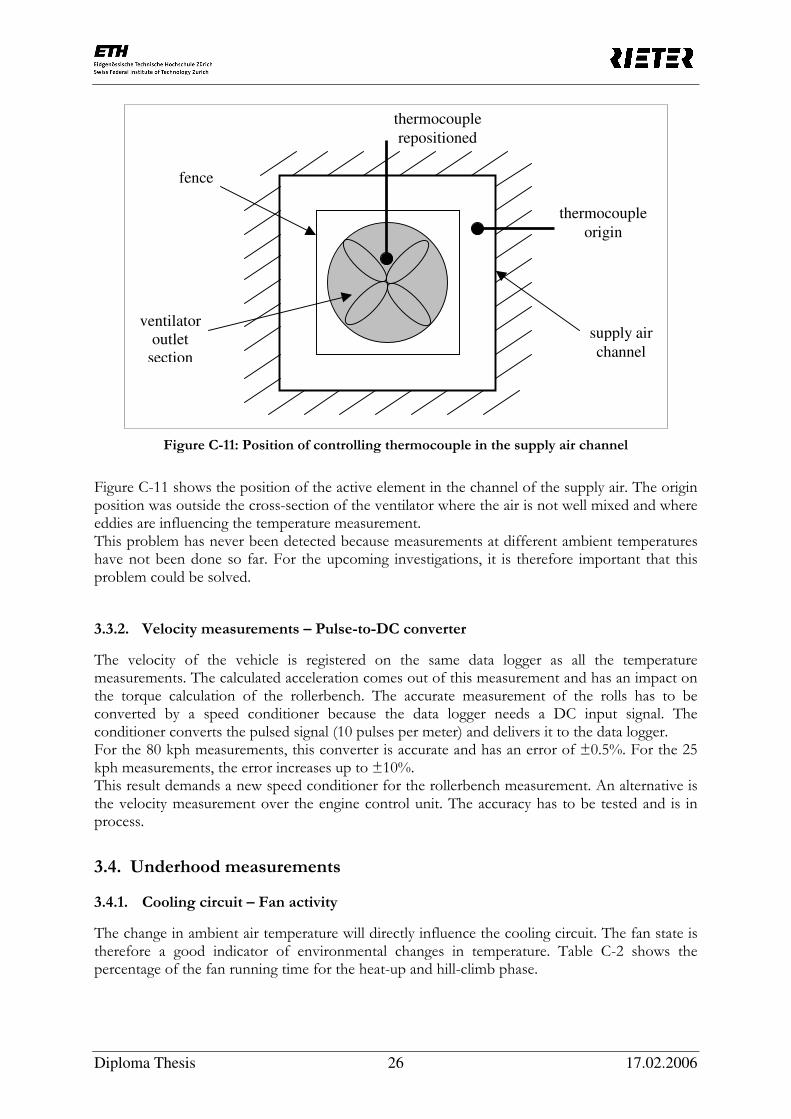
Figure C-11: Position of controlling thermocouple in the supply air channel
Figure C-11 shows the position of the active element in the channel of the supply air. The origin position was outside the cross-section of the ventilator where the air is not well mixed and where eddies are influencing the temperature measurement. This problem has never been detected because measurements at different ambient temperatures have not been done so far. For the upcoming investigations, it is therefore important that this problem could be solved.
3.3.2. Velocity measurements – Pulse-to-DC converter
The velocity of the vehicle is registered on the same data logger as all the temperature measurements. The calculated acceleration comes out of this measurement and has an impact on the torque calculation of the rollerbench. The accurate measurement of the rolls has to be converted by a speed conditioner because the data logger needs a DC input signal. The conditioner converts the pulsed signal (10 pulses per meter) and delivers it to the data logger. For the 80 kph measurements, this converter is accurate and has an error of ±0.5%. For the 25 kph measurements, the error increases up to ±10%. This result demands a new speed conditioner for the rollerbench measurement. An alternative is the velocity measurement over the engine control unit. The accuracy has to be tested and is in process.
3.4. Underhood measurements
3.4.1. Cooling circuit – Fan activity
The change in ambient air temperature will directly influence the cooling circuit. The fan state is therefore a good indicator of environmental changes in temperature. Table C-2 shows the percentage of the fan running time for the heat-up and hill-climb phase.
thermocouple
repositioned
supply air
channel
ventilator
outlet
section
fence
thermocouple
origin

Diploma Thesis 27 17.02.2006
temperature heat-up phase hill-climb test 12°C 33.12% 69.98% 16°C 34.31% 74.18% 20°C 37.40% 92.22% 24°C 42.21% 97.84% 28°C 46.65% 98.88%
Table C-2: Fan activity during the standard test
The engine power and the ambient air temperature are the driving parameters for the cycling behavior of the electric fan of the vehicle.
3.4.2. Tunnel entrance inlet temperatures
The underbody region is generally divided in different sections where the heatshield is placed. In front of these sections, the air temperature is measured at the tunnel entrance section. Figure C-12 shows the measurement positions. It is important to find out if there is an impact on the cooling circuit behavior for the tunnel entrance inlet temperature.
Figure C-12: Underbody sections with tunnel entrance
The temperature of the tunnel entrance air is important for a proper modeling of the underbody region. In Figure C-13, the measurement results are shown. A very strong dependency on the cooling system is observed. This is the main reason why underhood modeling is important before an underbody model can be built up. Without good correlation results of the underhood modeling, an underbody model will fail due to wrong initial conditions.
1 2 3 4
tunnel entrance

Diploma Thesis 28 17.02.2006
Figure C-13: Air temperatures at the tunnel entrance
The results show the intermediate state of the 20°C measurement. The fan frequency is changing with time. Air temperatures at the tunnel entrance position for the 20°C ambient measurement will be even lower than for the 16°C ambient measurement at the end of the hill-climb test.
3.4.3. Average gas manifold temperature
The gas manifold temperature calculation in the simulation chapter assumes that the behavior is linear to the engine power. To check if that is valid (without going to a detailed combustion calculation) for a given engine speed, measurements have been done on the rollerbench with different inclines from 2% to 12%.
Figure C-14: Gas manifold temperature for different engine load
Constant engine speed, changing load
200
250
300
350
400
450
500
0.0 5.0 10.0 15.0 20.0
engine power [kW]
gas m
an
ifo
ld t
em
pera
ture
[°C
]
1st gear Linear (1st gear)
Air temperature at tunnel entrance
70
75
80
85
90
95
100
3000 3200 3400 3600 3800 4000 4200 4400 4600 4800 5000
12°C ambient
16°C ambient
20°C ambient
24°C ambient
28°C ambient
Diploma Thesis 29 17.02.2006
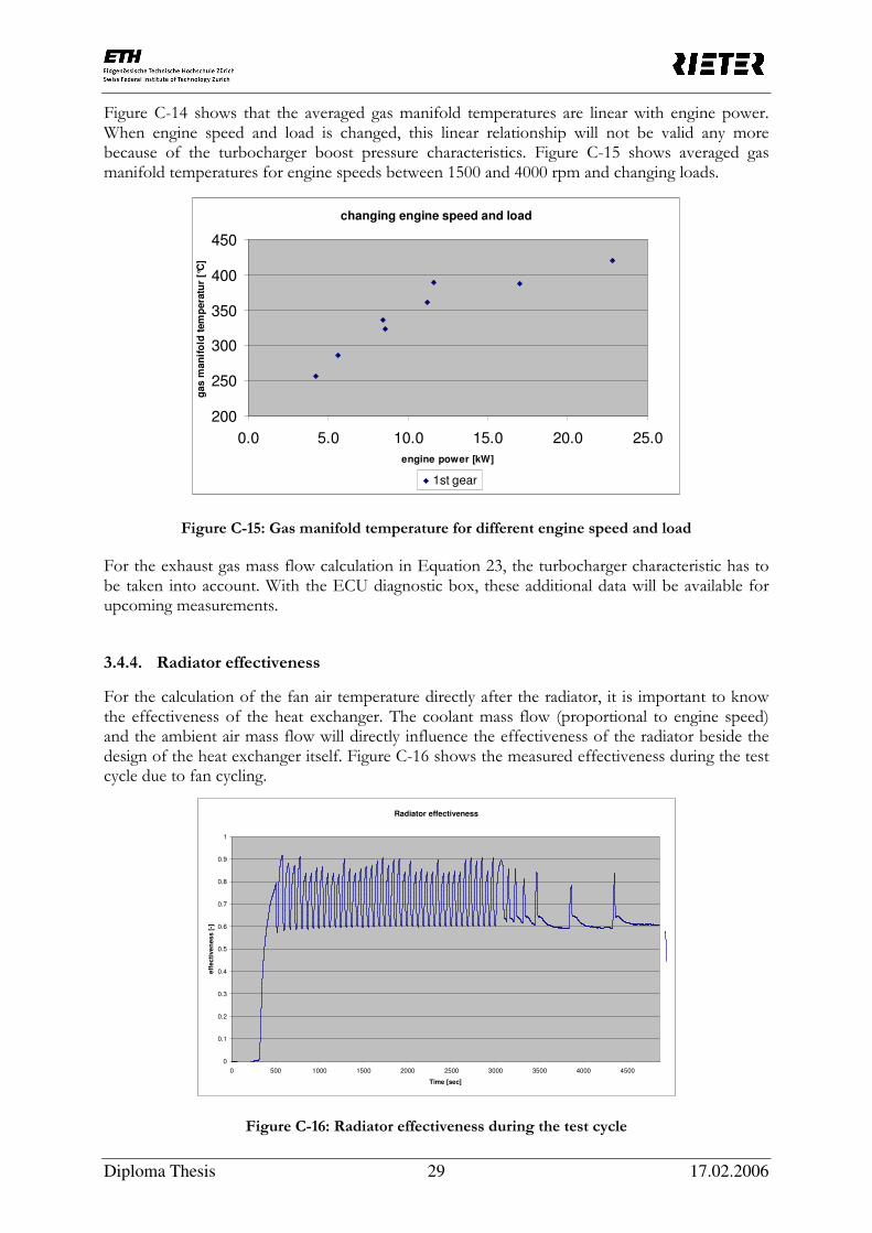
Figure C-14 shows that the averaged gas manifold temperatures are linear with engine power. When engine speed and load is changed, this linear relationship will not be valid any more because of the turbocharger boost pressure characteristics. Figure C-15 shows averaged gas manifold temperatures for engine speeds between 1500 and 4000 rpm and changing loads.
Figure C-15: Gas manifold temperature for different engine speed and load
For the exhaust gas mass flow calculation in Equation 23, the turbocharger characteristic has to be taken into account. With the ECU diagnostic box, these additional data will be available for upcoming measurements.
3.4.4. Radiator effectiveness
For the calculation of the fan air temperature directly after the radiator, it is important to know the effectiveness of the heat exchanger. The coolant mass flow (proportional to engine speed) and the ambient air mass flow will directly influence the effectiveness of the radiator beside the design of the heat exchanger itself. Figure C-16 shows the measured effectiveness during the test cycle due to fan cycling.
Figure C-16: Radiator effectiveness during the test cycle
changing engine speed and load
200
250
300
350
400
450
0.0 5.0 10.0 15.0 20.0 25.0
engine power [kW]
gas m
an
ifo
ld t
em
pera
tur
[°C
]
1st gear
Radiator effectiveness
0
0.1
0.2
0.3
0.4
0.5
0.6
0.7
0.8
0.9
1
0 500 1000 1500 2000 2500 3000 3500 4000 4500
Time [sec]
eff
ec
tive
nes
s [
-]

Diploma Thesis 30 17.02.2006
For the constant air speed of 23 kph, the radiator effectiveness cycles between the values 0.6 and 0.9. The effectiveness of the fins is therefore decreased when the fan cuts in. The radiator effectiveness of the Simulink/Matlab-model has to follow this behavior in order to correlate with the fan air temperature. It has to be noted that the effectiveness of the heat exchanger is not equal to the effectiveness of the fins. Detailed information regarding the effectiveness calculation can be found in the simulation chapter.
3.4.5. Thermostat behavior at the heat-up phase
Figure C-17 shows the coolant temperature once directly after the engine (measured in the bypass) and once right after the radiator. Before the thermostat is fully open at the operation temperature, it closes partly after the first opening. This is because the amount of coolant within the radiator circuit will lower the mixing temperature after the first cycle. When the coolant mass flow through the radiator is very low, the coolant can be fully cooled down to ambient temperature.
Figure C-17: Coolant temperature characteristics
To model this behavior, mass flow measurements have to be done as well as a map for the hysteresis of the expansion-element. Since the heat-up is not of great importance for the overall test cycle, direct comparison between the model and the measurements cannot be drawn until the first point, where the coolant reaches the fan-cut-in temperature. For a simulation of a stop-and-go cycle, the thermostat behavior will become important and the integration of the hysteresis will be essential.
3.5. Underbody measurements
Body, heatshield, exhaust surface, exhaust gas and air temperatures are measured in four sections of the underbody region. The influence of changing ambient air temperatures on the body can be seen in Figure C-18.
Coolant temperature behavior due to thermostat opening position
0
10
20
30
40
50
60
70
80
90
100
11:06:43 11:09:36 11:12:29 11:15:22 11:18:14 11:21:07 11:24:00
Radiator out
Engine coolant out

Diploma Thesis 31 17.02.2006
Section 1: Body temperatures
0
10
20
30
40
50
60
70
80
90
0 500 1000 1500 2000 2500 3000 3500 4000 4500 5000
12°C
16°C
20°C
24°C
28°C
Section 2: Body temperatures
0
10
20
30
40
50
60
70
80
0 500 1000 1500 2000 2500 3000 3500 4000 4500 5000
12°C
16°C
20°C
24°C
28°C
Section 3: Body temperatures
0
10
20
30
40
50
60
70
0 500 1000 1500 2000 2500 3000 3500 4000 4500 5000
12°C
16°C
20°C
24°C
28°C

Diploma Thesis 32 17.02.2006
Figure C-18: Body temperatures at different ambient air temperatures for all sections
Figure C-19 confirms that an underbody simulation has to be done and that it will not be possible for body temperatures to take the changing ambient air temperature by a constant into account. The cooling system will influence the underbody component temperature, because the heated-up ambient air has a direct impact on the convection between body and heatshield.
Figure C-19: Body temperature distribution at section 1 corrected by a constant temperature
For heatshield and further temperatures in the underbody region, this effect is much stronger because of the lower inertia compared to the body. Additionally, the down drifting ambient temperature will have an influence on the shape of the curves. It has been waived to show all the temperature characteristics of the different components in the underbody region. The dependency on cooling system behavior has been approved for all measurement tests.
Section 1: Body temperatures corrected (constant delta T)
0
10
20
30
40
50
60
70
80
0 500 1000 1500 2000 2500 3000 3500 4000 4500 5000
12°C
16°C
20°C
24°C
28°C
Section 4: Body temperatures
0
10
20
30
40
50
60
70
0 500 1000 1500 2000 2500 3000 3500 4000 4500 5000
12°C
16°C
20°C
24°C
28°C

Diploma Thesis 33 17.02.2006
D. Derivation of a 1-D thermal model
1. Introduction
The previous chapters have shown the occurring problems of the on-road tests. It has also been explained why it was necessary to do further rollerbench tests to understand properly the different temperature behavior. Since the test facility was occupied until the end of December, a numerical simulation was pushed forward. First, an explicit temperature calculation was done using Matlab, without solving the different equations simultaneously. In a second stage, a new model was built up in Simulink/Matlab to avoid the occurred problems of the first stage Matlab-model.
2. 1-D transient underhood modeling
For the investigation of the underbody region, it is necessary to understand as well the thermal management of the underhood. This is because the temperatures in the engine compartment will influence strongly the transient behavior of the components in the underbody region. It is therefore inevitable to simulate as well the underhood components. This task can be done in several ways; one of them is the one-dimensional fluid dynamic modeling. It represents the flow and heat transfer of the whole cooling system in a simplified manner but it does not take into account the exact geometry of the vehicle. An energy balance will determine the heat rejection by the engine, heat transfer to the coolant, oil and ambient air. For a proper model, the engine block, the oil cooler and the radiator have to be investigated in more detail. The goal is to match the predicted coolant temperature with the experimental data. Figure D-1 shows the cooling system arrangement of the investigated vehicle.
Figure D-1: Cooling system of the vehicle: 1. cooling water pump, 2. temperature sender to the display and error lamp, 3. temperature sensor for engine coolant, 4. thermostat, 5. radiator,
6. electric fan, 7. expansion tank, 8. pipe junction leading to the water pump, 9. oil-water heat exchanger, 10. vehicle heater
Diploma Thesis 34 17.02.2006
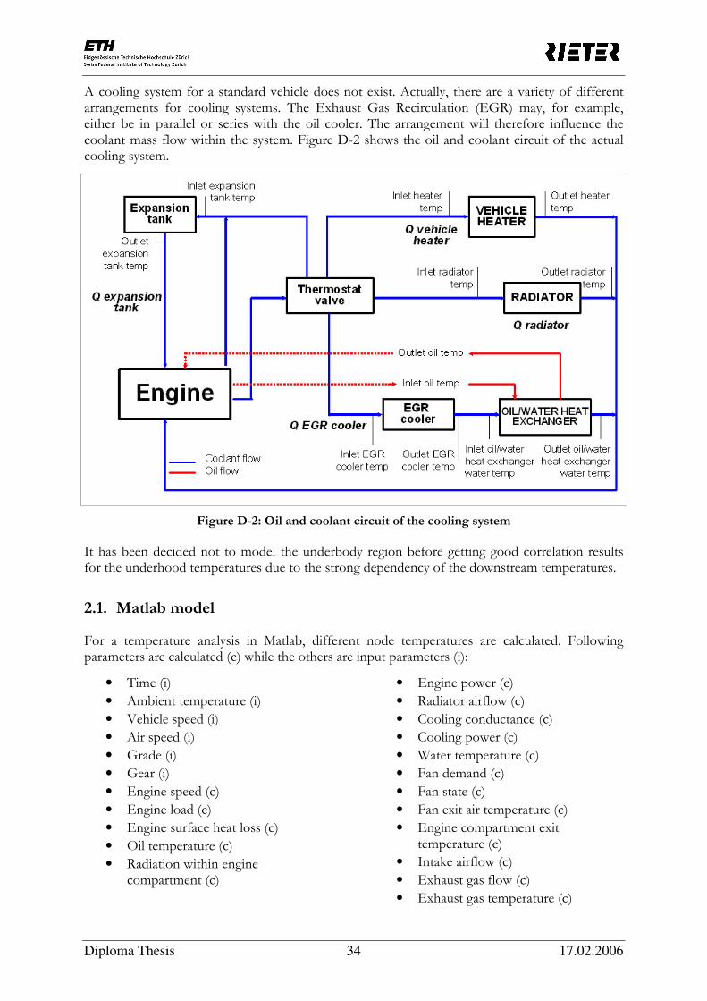
A cooling system for a standard vehicle does not exist. Actually, there are a variety of different arrangements for cooling systems. The Exhaust Gas Recirculation (EGR) may, for example, either be in parallel or series with the oil cooler. The arrangement will therefore influence the coolant mass flow within the system. Figure D-2 shows the oil and coolant circuit of the actual cooling system.
Figure D-2: Oil and coolant circuit of the cooling system
It has been decided not to model the underbody region before getting good correlation results for the underhood temperatures due to the strong dependency of the downstream temperatures.
2.1. Matlab model
For a temperature analysis in Matlab, different node temperatures are calculated. Following parameters are calculated (c) while the others are input parameters (i):
• Time (i)
• Ambient temperature (i)
• Vehicle speed (i)
• Air speed (i)
• Grade (i)
• Gear (i)
• Engine speed (c)
• Engine load (c)
• Engine power (c)
• Radiator airflow (c)
• Cooling conductance (c)
• Cooling power (c)
• Water temperature (c)
• Fan demand (c)
• Fan state (c)
• Fan exit air temperature (c)
• Engine surface heat loss (c)
• Oil temperature (c)
• Radiation within engine compartment (c)
• Engine compartment exit temperature (c)
• Intake airflow (c)
• Exhaust gas flow (c)
• Exhaust gas temperature (c)

Diploma Thesis 35 17.02.2006
The first four parameters can be handed over so that any driving cycle can be simulated. The cycle starts with a heat-up phase followed by the hill-climb phase and ends with the soak phase. The information about topography can be inserted as well as actual ambient temperatures. Beside additional guessing parameters, the following parameters have been used to do an appropriate calculation:
• Aerodynamic drag
• Rolling resistance
• Train mass
• Cross-section area
• Coolant mass
• Engine mass
• Fan cut in and cut out temperatures
• Radiator airflow with running fan
• Thermostat temperature
• Radiator area
• Radiator effectiveness
• Gear ratios
• Thermal budget factors
• Oil to water conductance
The Matlab code for the explicit temperature calculation is shown in Chapter 12. The following time-steps can be chosen: 0.1, 1, 5, or 10 seconds. It is necessary to lower the time-step down to at least one second to avoid any overshooting of the simulated coolant temperature that is limited by the fan control unit due to numerical integration reasons. Figure D-3 shows one result for the water, oil and fan exit air temperature compared to the measured data.
Figure D-3: Simulated and measured cooling system temperatures
The heat transfer coefficient calculation is based on the boundary theory over a plane wall for five underbody sections. The Matlab code is shown in Chapter 12. For underbodies with a smooth surface (e.g. covering), this is a reasonable approximation for the investigation. The laminar as well as the turbulent region have been taken into account.

Diploma Thesis 36 17.02.2006
The following relationships have been used:
Dimensionless numbers:
µ
ρ
ν
LULUL
⋅⋅=
⋅=Re
k
LhNu L
L
⋅=
κ
ν=Pr
The value of Lh depends on how the transition length xtr compares with the total length L:
⋅+⋅= ∫∫ dxhdxh
Lh
L
x
x
x
lxL
tr
tr
turbulentaminar ,
0
,
1 (Eq. 1)
Critical Reynolds number: 5
,, 105Re ⋅≈platecriticalx
The critical Reynolds number is used for a first calculation of the heat transfer coefficient. In the case of underbody simulation, this number is shifted towards smaller values because the existing geometry will force the flow to get turbulent in an earlier stage compared to a flat plate.
Turbulent Prandtl number ([X]): 85.0Pr ≈turbulent
The turbulence model used for the temperature field is based on the concept of the constant turbulent Prandtl number. According to this turbulence model, the turbulent Prandtl number is not only constant in the overlap layer, but also in the entire core layer. Laminar boundary layer ([3], [6]):
Momentum boundary layer thickness: xxl ⋅⋅≈−
2
1
Re92.4δ (Eq. 2)
Thermal boundary layer thickness: 3
1
Pr−
⋅≈ lTlδδ (Eq. 3)
Average Nusselt number: 3
1
2
1
PrRe664.0 ⋅⋅≈ LLNu , 5.0Pr ≥ (Eq. 4)
( )2
1
PrRe128.1 ⋅⋅≈ LLNu , 5.0Pr ≤ (Eq. 5)
Turbulent boundary layer ([3], [6]):
Momentum boundary layer thickness: xxt ⋅⋅≈−
5
1
Re37.0δ (Eq. 6)
Thermal boundary layer thickness: 3
1
Pr−
⋅≈ turbulenttTtδδ (Eq. 7)
Average Nusselt number:
−⋅⋅+⋅⋅≈ 5
4
,5
43
1
2
1
,3
1
ReRePr037.0RePr664.0 criticalxLcriticalxLNu (Eq. 8)
−⋅⋅≈ 550'23RePr037.0 5
43
1
LLNu , platecriticalxcriticalx ,,, ReRe = (Eq. 9)
The heat transfer coefficient h for each of the five sections in the underbody region has been calculated in dependency of the local speed. With this information, heat transfer coefficient curves are built up for a later transfer to the underbody model. This modeling is essential because of the different boundary layer behavior in the underbody region at different driving speeds. Figure D-4 shows a typical behavior of the boundary layer where a transition from laminar to turbulent flow is occurring between the second and third section of the model at 25 kph. For higher driving speeds, the transition position is shifting towards the front edge and the heat transfer coefficients are changing considerably. For higher velocities, the impact will be even stronger.

Diploma Thesis 37 17.02.2006
Figure D-4: Heat transfer coefficient calculation for underbody boundary layer
Looking at the boundary layer thickness of the momentum and thermal boundary layer in Figure D-5, one sees clearly that the transition will have an influence on the heat transfer coefficient. The transition phase is not modeled assuming a short length of transition.
Figure D-5: Boundary layer thickness of flat plate
The following statements can be done for the first Matlab-model:
• The transient behavior of the oil temperature cannot be modeled properly.
• The fan state can be simulated: In the first phase, the fan is cycling with almost the same frequency like in the measured data and in the second phase, the fan keeps running without cutting out.
• The simulation is not able to correlate the fan air exit temperature. An additional node for the radiator fin temperature has to be introduced taking into account the heat exchanger behavior for different flow rates.
• The transition from the first to the second phase does not represent the real behavior.
• The results until the water temperature (coolant) has reached the fan-cut-in temperature cannot be compared to the measured data. The reason for that is that the thermocouples have to be positioned once directly after the radiator and once in the bypass of the cooling
heat transfer coefficient calculation
0
5
10
15
20
25
0 1 2 3 4 5 6
section number
heat
tran
sfe
r co
eff
icie
nt
[W/m
^2K
]
h_sector (of entire BL)
boundary layer thickness of flat plate
0
0.01
0.02
0.03
0.04
0.05
0.06
0.07
0 0.5 1 1.5 2 2.5 3
distance to front edge [m]
bo
un
da
ry l
ay
er
thic
kn
es
s [
m]
Momentum
Thermal
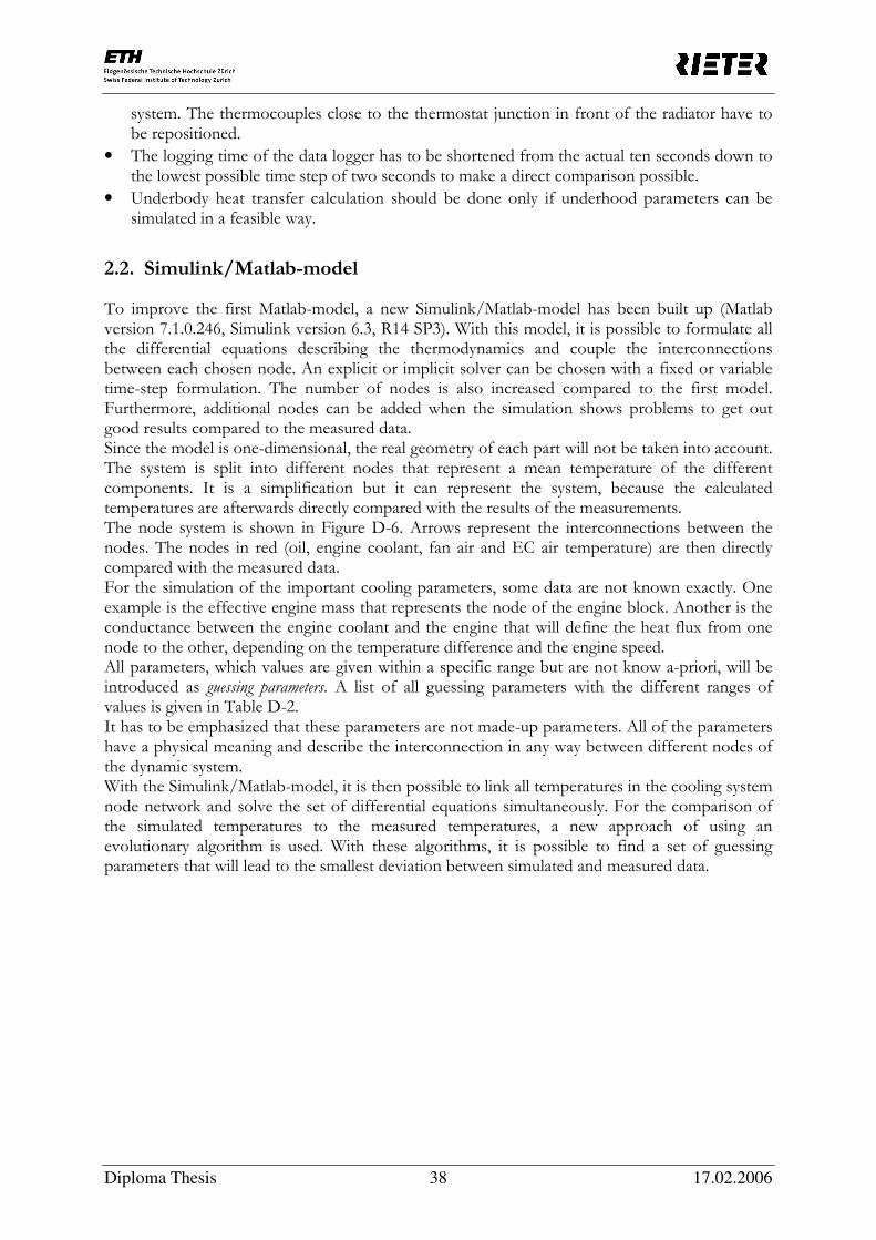
Diploma Thesis 38 17.02.2006
system. The thermocouples close to the thermostat junction in front of the radiator have to be repositioned.
• The logging time of the data logger has to be shortened from the actual ten seconds down to the lowest possible time step of two seconds to make a direct comparison possible.
• Underbody heat transfer calculation should be done only if underhood parameters can be simulated in a feasible way.
2.2. Simulink/Matlab-model
To improve the first Matlab-model, a new Simulink/Matlab-model has been built up (Matlab version 7.1.0.246, Simulink version 6.3, R14 SP3). With this model, it is possible to formulate all the differential equations describing the thermodynamics and couple the interconnections between each chosen node. An explicit or implicit solver can be chosen with a fixed or variable time-step formulation. The number of nodes is also increased compared to the first model. Furthermore, additional nodes can be added when the simulation shows problems to get out good results compared to the measured data. Since the model is one-dimensional, the real geometry of each part will not be taken into account. The system is split into different nodes that represent a mean temperature of the different components. It is a simplification but it can represent the system, because the calculated temperatures are afterwards directly compared with the results of the measurements. The node system is shown in Figure D-6. Arrows represent the interconnections between the nodes. The nodes in red (oil, engine coolant, fan air and EC air temperature) are then directly compared with the measured data. For the simulation of the important cooling parameters, some data are not known exactly. One example is the effective engine mass that represents the node of the engine block. Another is the conductance between the engine coolant and the engine that will define the heat flux from one node to the other, depending on the temperature difference and the engine speed. All parameters, which values are given within a specific range but are not know a-priori, will be introduced as guessing parameters. A list of all guessing parameters with the different ranges of values is given in Table D-2. It has to be emphasized that these parameters are not made-up parameters. All of the parameters have a physical meaning and describe the interconnection in any way between different nodes of the dynamic system. With the Simulink/Matlab-model, it is then possible to link all temperatures in the cooling system node network and solve the set of differential equations simultaneously. For the comparison of the simulated temperatures to the measured temperatures, a new approach of using an evolutionary algorithm is used. With these algorithms, it is possible to find a set of guessing parameters that will lead to the smallest deviation between simulated and measured data.

Diploma Thesis 39 17.02.2006
Figure D-6: Node system of the 1-D model
Heat going to the exhaust gas, the engine oil and the engine coolant has a different origin. While heat to oil is mainly driven by friction and therefore engine speed dependent, heat to engine coolant and gas is proportional to the engine power for a specific engine speed.
2.2.1. Motor-vehicle dynamics – Engine calculation
Engine parameters are calculated as followed:
Engine speed:
axisgear
wheel
rrp
vn ⋅⋅= (Eq. 10)
Engine load:
ams
gmv
cgmcvA
FFFFF
RD
graderolldrag
⋅+
⋅⋅+
+⋅⋅⋅+⋅⋅⋅⋅=
+++=
100arctansin
10001
2
1 *2
intertia
ρ (Eq. 11)
Engine power:
vFP ⋅= (Eq. 12)
The calculation of the engine parameters is essential for the further calculation of the cooling system. The engine power is the required power that must be transmitted through the drive wheels to overcome running resistance.
HEAT
exhaust gas oil engine
coolant
engine block
radiator coolant
EC air
exhaust surface
fin
ambient
fan air
boundary condition for underbody
calculation
ambient
HEAT
exhaust gas oil engine
coolant
engine block
radiator coolant
EC air
exhaust surface
fin
ambient
fan air
boundary condition for underbody
calculation
ambient

Diploma Thesis 40 17.02.2006
The rolling resistance Froll is the product of deformation processes that occur at the contact patch between tire and road surface. Equation 11 shows that there is also a velocity dependency of the rolling resistance that comes out of rollerbench measurements made in the past. The acceleration resistance is only important for a short period at the beginning of the heat-up and hill-climb phase. The exact formula is:
minertia kamF ⋅⋅= (Eq. 13)
where km is the inertia coefficient, compensating for the apparent increase in vehicle mass due to the rotating masses (e.g. wheels, flywheel, crankshaft etc.). Figure D-7 shows the determination of the rotational inertia coefficient. km is dependant of the vehicle mass m, engine swept volume VH, gear ratio i and radius of tire r.
The mass to engine swept volume ratio is: l
kg
V
m
H
942≈
Figure D-7: Rotational inertia coefficient, [5]
Gear 1 2 3 4 5 gear ratio [-] 12.73 7.50 4.56 3.25 2.55
0.3⋅i/r [m-1] 6.21 3.66 2.22 1.59 1.24
Table D-1: Determining the rotational inertia coefficient
Figure D-7 shows with Table D-1 that in our case, the rotational inertia coefficient will not
exceed the value km ≅1.05 for all five gears. The influence of the inertia coefficient will therefore be neglected. Engine power versus wheel power: For an exact measurement of the frictional losses in the drivetrain and tires, accurate engine dynamometer tests as well as rolling road dynamometer tests have to be done. This is because some portion of the flywheel power will be lost in the gearbox, final drive, drive shaft bearings, wheel bearings and tires. It is true that not every component in a transmission system absorbs a fixed percentage of the input power, but to a large extent the dependency goes on the amount of power being fed into the transmission. Since the heat input is calculated by a given ratio to engine power by a guessing parameter, the transmission losses will already be included for the further calculation (e.g. around 15% for an average front wheel drive car). For a very broad engine speed regime (we measure only between 1750 and 2750 rpm), the proportionality assumption is not valid any more.

Diploma Thesis 41 17.02.2006
Simulink model:
Figure D-8: Engine calculation subsystem
Figure D-9: Load calculation subsystem
Rollerbench power train
For all rollerbench measurements, there is an important issue regarding the power train for the engine load calculation. If the power train is turned off, only a rolling resistance is present (neglecting the acceleration of the rollers and the bearing losses). Drag resistance, grade resistance and inertia resistance do not exist. The rolling resistance at that point is doubled compared to the actual resistance on the road. The reason for that is the position of each vehicle tire between two rollers. The contact surface is doubled and therefore the resistance as well. By typing in a value for the coefficient of rolling resistance, the additional rolling resistance is compensated by the control unit. For that, a value for mechanical losses cL is deposited which will take into account this transition from the laboratory to the road.
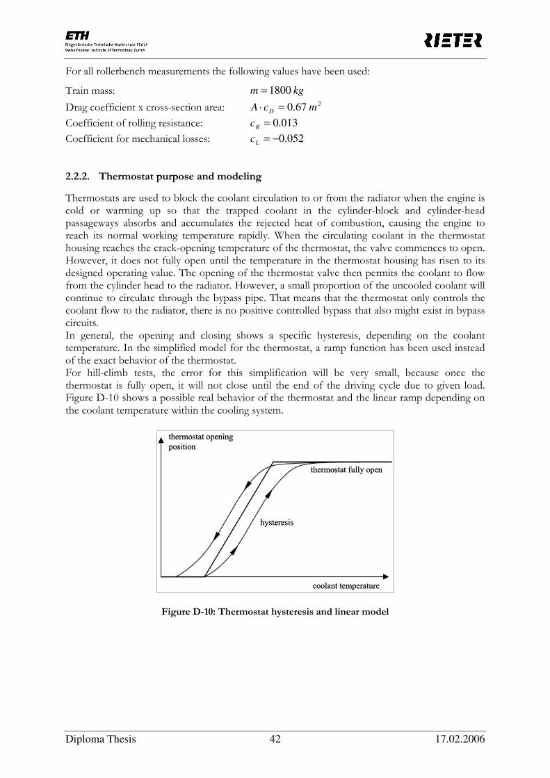
Diploma Thesis 42 17.02.2006
For all rollerbench measurements the following values have been used:
Train mass: kgm 1800=
Drag coefficient x cross-section area: 2 67.0 mcA D =⋅
Coefficient of rolling resistance: 013.0=Rc
Coefficient for mechanical losses: 052.0−=Lc
2.2.2. Thermostat purpose and modeling
Thermostats are used to block the coolant circulation to or from the radiator when the engine is cold or warming up so that the trapped coolant in the cylinder-block and cylinder-head passageways absorbs and accumulates the rejected heat of combustion, causing the engine to reach its normal working temperature rapidly. When the circulating coolant in the thermostat housing reaches the crack-opening temperature of the thermostat, the valve commences to open. However, it does not fully open until the temperature in the thermostat housing has risen to its designed operating value. The opening of the thermostat valve then permits the coolant to flow from the cylinder head to the radiator. However, a small proportion of the uncooled coolant will continue to circulate through the bypass pipe. That means that the thermostat only controls the coolant flow to the radiator, there is no positive controlled bypass that also might exist in bypass circuits. In general, the opening and closing shows a specific hysteresis, depending on the coolant temperature. In the simplified model for the thermostat, a ramp function has been used instead of the exact behavior of the thermostat. For hill-climb tests, the error for this simplification will be very small, because once the thermostat is fully open, it will not close until the end of the driving cycle due to given load. Figure D-10 shows a possible real behavior of the thermostat and the linear ramp depending on the coolant temperature within the cooling system.
Figure D-10: Thermostat hysteresis and linear model

Diploma Thesis 43 17.02.2006
Simulink model:
Figure D-11: Thermostat position subsystem
2.2.3. Fan modeling
The vehicle fan is very important for the cooling system. The fan demand and the fan state will be calculated depending on the temperature of the engine coolant. Most of the automobiles have two-stage electric fans with different fan-cut-in and fan-cut-out temperatures. For the calculation of the fan demand, the two fan-cut-in temperatures and the engine coolant temperature have to be known. The fan can either be demanded or not demanded. For the fan state calculation, the last fan state, the fan demand and the two fan-cut-off temperatures have to be known additionally. The fan state is either turned off, running at low speed or running at high speed. Figure D-12 shows the calculation of the fan state.
Figure D-12: Fan state calculation
Fan demand
Last fan state = 0 0
Tw < fan_cut_out1 0
Tw < fan_cut_out2 1
2
Last fan state = 2 1
Tw < fan_cut_out2 2
1
2
0 1 2
yes
yes
yes
no
no
no
no
no
yes
yes

Diploma Thesis 44 17.02.2006
Simulink model:
Figure D-13: Overview: Fan demand, fan state and thermostat position
Figure D-14: Fan demand subsystem
Figure D-15: Radiator airflow subsystem

Diploma Thesis 45 17.02.2006
2.2.4. Thermodynamic balance
The thermodynamic balance within the engine compartment is dependent on many parameters, mainly on vehicle load and speed. The main contributors for heat dissipation are heat to coolant, heat to exhaust gas, heat to oil and dissipation by convection and radiation. Figure D-16 shows the heat balance of an engine test for a load of 20%. The amount of dissipation by the vehicle heater is very small; dissipation to EGR cooler is small in the high revs, but increases when the engine speed is low.
Figure D-16: Thermodynamic balance of heat dissipation
For the Simulink-model, the amount of heat to engine coolant and exhaust gas depends linearly on the engine power, while the amount of heat to oil depends linearly on the engine speed. This is a rough assumption, but for tests within a certain limit in engine speed it represents in a simplified way the heat fluxes to the different fluid nodes. Dissipation to the vehicle heater does not have to be taken into account, because no tests are done with the engine heater turned on. The effect of the exhaust gas recirculation is small for the higher power range. It has been neglected due to the fact that no detailed information about the mass flow regulation is available. For a better understanding of the control system of the vehicle, an Engine Control Unit (ECU) diagnostic box has been acquired. Accurate information about engine speed, waste gate valve position, internal boost pressure etc. can be delivered and the functionality of the exhaust gas recirculation or the intercooler can be properly understood.
2.2.5. Thermodynamic equations
The following equations correspond to Figure D-6 and describe the heat fluxes from one node to the other. Every node represents an origin of heat transfer. Besides the coupling of nodes, there are also advection links, which represent an input for a different node. Beside physical properties of the nodes, there are guessing parameters introduced which correspond to an exchange between two nodes.
0%
10%
20%
30%
40%
50%
60%
70%
80%
90%
100%
4750 4500 4250 4000 3750 3500 3250 3000 2750 2500 2250 2000 1750 1500 1250
Thermodynamic balance 1910 JTD (20%)
useful power power dissipated by oil power dissipated by coolant
power dissipated by vehicle heater power dissipated by exhaust gas power dissipated by egr cooler
power dissipated by convection and radiation

Diploma Thesis 46 17.02.2006
Since the node system does not take into account the real geometry of the component, the physical properties stand for an averaged property of the node having a uniform temperature distribution. Engine coolant:
( )
( )( )
enginecoolantheat
coolantengcoolantradcoolantengcoolantrad
coolantengoilcoolantengoil
coolantengengineenginecoolanteng
coolanteng
coolantengp
Pf
vTTnC
TTnC
TTnCdt
dTcm
⋅+
⋅−⋅⋅+
−⋅⋅+
−⋅⋅=⋅⋅
2
_____
___
___
_
_][
(Eq. 14)
Engine oil:
( )
( )
( )
nf
gTTNuAL
k
TTnC
TTnCdt
dTcm
oilheat
oilsumpoilairECfpLoilsump
oilsump
air
oilengineengineoil
oilcoolantengcoolantengoiloil
oilp
⋅+
⋅−⋅⋅⋅+
−⋅⋅+
−⋅⋅=⋅⋅
2
_,
_
___][
(Eq. 15)
Engine block:
( )
( )
( )engineengineairECfpLengine
engine
air
enginecoolantengenginecoolanteng
engineoilengineoil
engine
enginep
gTTNuAL
k
TTnC
TTnCdt
dTcm
⋅−⋅⋅⋅+
−⋅⋅+
−⋅⋅=⋅⋅
_,
___
_][
(Eq. 16)
with 3
1
2
1
, PrRe664.0 ⋅⋅= LfpLNu
( )
( )
( ) 2
1
_
2
1
3
1
___
_
Pr664.0
][
fanengineengineairEC
engineair
airengineair
enginecoolantengenginecoolanteng
engineoilengineoil
engine
enginep
ugTTL
Ak
TTnC
TTnCdt
dTcm
⋅⋅−⋅
⋅⋅⋅⋅⋅+
−⋅⋅+
−⋅⋅=⋅⋅
µ
ρ
Radiator coolant:
( )
( ) vTTnC
vTTnCdt
dTcm
coolantradfinfincoolantrad
coolantradcoolantengcoolantradcoolanteng
coolantrad
coolantradp
⋅−⋅⋅+
⋅−⋅⋅=⋅⋅
___
_____
_
_][ (Eq. 17)
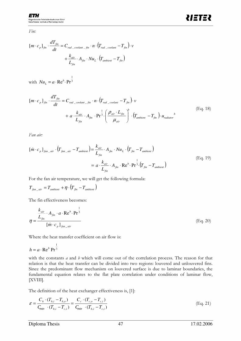
Diploma Thesis 47 17.02.2006
Fin:
( )
( )finambientLfin
fin
air
fincoolantradfincoolantrad
fin
finp
TTNuAL
k
vTTnCdt
dTcm
−⋅⋅⋅+
⋅−⋅⋅=⋅⋅ ___][
with 3
1
PrRe ⋅⋅= b
L aNu
( )
( ) b
radiatorfinambient
b
air
finair
fin
fin
air
fincoolantradfincoolantrad
fin
finp
uTTL
AL
ka
vTTnCdt
dTcm
⋅−⋅
⋅⋅⋅⋅⋅+
⋅−⋅⋅=⋅⋅
µ
ρ3
1
___
Pr
][
(Eq. 18)
Fan air:
( ) ( )
( )ambientfin
b
fin
fin
air
ambientfinLfin
fin
air
ambientairfanairfanp
TTAL
ka
TTNuAL
kTTcm
−⋅⋅⋅⋅⋅=
−⋅⋅⋅=−⋅⋅
3
1
__
PrRe
][ &
(Eq. 19)
For the fan air temperature, we will get the following formula:
( )ambientfinambientairfan TTTT −⋅+= η_
The fin effectiveness becomes:
airfanp
b
fin
fin
air
cm
aAL
k
_
3
1
][
PrRe
⋅
⋅⋅⋅⋅
=&
η (Eq. 20)
Where the heat transfer coefficient on air flow is:
3
1
PrRebah ⋅=
with the constants a and b which will come out of the correlation process. The reason for that relation is that the heat transfer can be divided into two regions: louvered and unlouvered fins. Since the predominant flow mechanism on louvered surface is due to laminar boundaries, the fundamental equation relates to the flat plate correlation under conditions of laminar flow, [XVIII]. The definition of the heat exchanger effectiveness is, [1]:
)(
)(
)(
)(
,,
,,
,,
,,
icih
icocc
icih
ohihh
TTC
TTC
TTC
TTC
−⋅
−⋅=
−⋅
−⋅=
minminε (Eq. 21)

Diploma Thesis 48 17.02.2006
cpcc cmC ,⋅= &
hphh cmC ,⋅= &
),min( hc CCC =min
where Th,i and Th,o are the inlet and outlet temperatures of the hot fluid and Tc,i and Tc,o are the inlet and outlet temperatures of the cold fluid.
Figure D-17: Limitation of fin effectiveness
The fin effectiveness has a theoretical maximum of η=1. This is the case when the fan air temperature will exactly reach the temperature of the fin. It has to be checked that the fin effectiveness does not exceed this level. The fin effectiveness is a ratio built of empirical and exact values; therefore, this constraint is not automatically fulfilled. The radiator itself is coolant side limited, that means that for all operation points of the heat exchanger, the minimum conductance Cmin will be equal to the coolant side conductance Cc. The defined effectiveness of the radiator becomes:
ambientinradiator
ambientairfan
TT
TT
−
−=
_
_ε
The effective inlet radiator temperature is not equal to the radiator coolant, because the latter describes the mean temperature of the open-loop circuit. The fin effectiveness is:
1_ −⋅∝
⋅
⋅∝
−
−=
b
rad
p
b
rad
ambientfin
ambientairfanua
cm
ua
TT
TT
&η (Eq. 22)
This relationship is valid for the open thermostat and for the forced convection taking place at the fins. When the airflow is stopped completely (no fan activation, stopped vehicle, no external wind), the heat is only rejected by natural convection at the fins and Equation 19 will not be valid any more. Exhaust gas:
( )enginegasexhheatambientgasexhgasexhp PfTTcm ⋅=−⋅⋅ _2__][ &
For the exhaust gas temperature, we will get the following formula:
gasexhp
enginegasexhheat
ambientgasexhcm
PfTT
_
_2
_][ ⋅
⋅+=
& (Eq. 23)
η
v
1 theoη
realη

Diploma Thesis 49 17.02.2006
with fuelair
H
gasexh rVn
m ⋅⋅⋅⋅
⋅= ρ
6010002_
& for non-turbocharged four-stroke engines.
Exhaust:
For the exhaust Nusselt number, empirical formulas are available and differ slightly form the empirical formula for turbulent flow in smooth pipes. Following correlations can be found in [XIII]:
5
2
5
4
PrRe023.0 ⋅⋅=DBNu Dittus-Boelter (fully-developed turbulent flow in smooth pipes)
3
1
5
4
PrRe023.0 ⋅⋅=CNu Colburn (fully-developed turbulent flow in smooth pipes)
713.0Re0675.0 ⋅=MFNu Martins and Finlay (intake flow)
769.0Re0774.0 ⋅=MSNu Meisner-Sorenson (exhaust flow)
( ) ( )airECexhexhoutflowexhexhgasexhexhexh_inflowexh_inflow TTAhTTAhg ___ −⋅⋅=−⋅⋅⋅
with
exh
gasexh
exh
gasexh
MSexh_inflowd
k
d
kNuh
_769.0_Re0774.0 ⋅⋅=⋅=
gasexh
exh
gasexhgasexhgasexhgasexhgasexh ud
uAm _
2
_____4
⋅⋅⋅=⋅⋅= πρρ&
)(, ___ gasexhgasexhgasexh Tfk =µ
and
exh
aird
exh
airwexh_outflo
d
kc
d
kNuh ⋅⋅⋅=⋅= 3
1
PrRe
For the two conductances for each side we will get:
exh
gasexhexh
gasexh
gasexhexhexh_inflow Ld
mkAh ⋅⋅
⋅
⋅⋅⋅=⋅ 231.0
769.0
_
_
_
40774.0 π
µ
&
exh
d
air
exhfanair
airexhwexh_outflo Ldu
kcAh ⋅⋅⋅
⋅⋅⋅⋅=⋅ π
µ
ρ3
1
Pr
Finally, we will get for the exhaust temperature the following expression:
exh_inflowexh_inflowoutflowexh
outflowexhairECexh_inflowexh_inflowgasexh
exhhgh
hThgTT
⋅+
⋅+⋅⋅=
_
___ (Eq. 24)
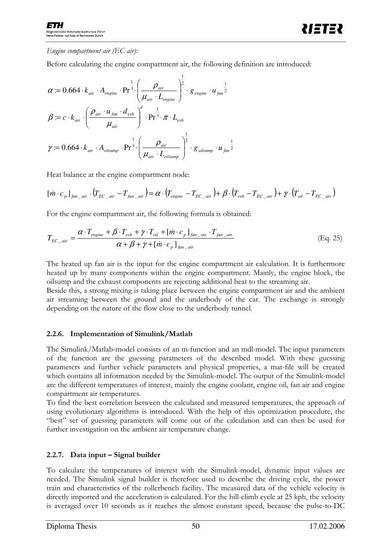
Diploma Thesis 50 17.02.2006
Engine compartment air (EC air):
Before calculating the engine compartment air, the following definition are introduced:
2
12
1
3
1
Pr664.0: fanengine
engineair
air
engineair ugL
Ak ⋅⋅
⋅⋅⋅⋅⋅=
µ
ρα
exh
d
air
exhfanair
air Ldu
kc ⋅⋅⋅
⋅⋅⋅⋅= π
µ
ρβ 3
1
Pr:
2
12
1
3
1
Pr664.0: fanailsump
oilsumpair
air
oilsumpair ugL
Ak ⋅⋅
⋅⋅⋅⋅⋅=
µ
ργ
Heat balance at the engine compartment node:
( ) ( ) ( ) ( )airECoilairECexhairECengineairfanairECairfanp TTTTTTTTcm ______][ −⋅+−⋅+−⋅=−⋅⋅ γβα&
For the engine compartment air, the following formula is obtained:
airfanp
airfanairfanpoilexhengine
airECcm
TcmTTTT
_
__
_][
][
⋅+++
⋅⋅+⋅+⋅+⋅=
&
&
γβα
γβα (Eq. 25)
The heated up fan air is the input for the engine compartment air calculation. It is furthermore heated up by many components within the engine compartment. Mainly, the engine block, the oilsump and the exhaust components are rejecting additional heat to the streaming air. Beside this, a strong mixing is taking place between the engine compartment air and the ambient air streaming between the ground and the underbody of the car. The exchange is strongly depending on the nature of the flow close to the underbody tunnel.
2.2.6. Implementation of Simulink/Matlab
The Simulink/Matlab-model consists of an m-function and an mdl-model. The input parameters of the function are the guessing parameters of the described model. With these guessing parameters and further vehicle parameters and physical properties, a mat-file will be created which contains all information needed by the Simulink-model. The output of the Simulink-model are the different temperatures of interest, mainly the engine coolant, engine oil, fan air and engine compartment air temperatures. To find the best correlation between the calculated and measured temperatures, the approach of using evolutionary algorithms is introduced. With the help of this optimization procedure, the “best” set of guessing parameters will come out of the calculation and can then be used for further investigation on the ambient air temperature change.
2.2.7. Data input – Signal builder
To calculate the temperatures of interest with the Simulink-model, dynamic input values are needed. The Simulink signal builder is therefore used to describe the driving cycle, the power train and characteristics of the rollerbench facility. The measured data of the vehicle velocity is directly imported and the acceleration is calculated. For the hill-climb cycle at 25 kph, the velocity is averaged over 10 seconds as it reaches the almost constant speed, because the pulse-to-DC

Diploma Thesis 51 17.02.2006
converter shows fluctuations in the range of 4 kph even if the velocity is held completely constant. The measured distribution of the ambient air temperature is also imported because the test facility showed difficulties in keeping the supply air temperature constant. The averaged air speed at the cross-section of the blower is 18 kph but the velocity at the radiator grill inlet position is 23 kph and slightly fluctuating. The power train value describes whether the power train is turned on or off. This is very important for the load calculation of the vehicle. Figure D-18 shows the signal builder with its values.
Figure D-18: Simulink signal builder
2.2.8. Simulink solver
For the calculation of the Simulink model, a fixed-step continuous solver has been chosen. To avoid too small time-steps or any unstable solution, an implicit solver with a time-step of one second was used. This solver computes the state at the next time step as an implicit function of the state derivative at the next time step, e.g.,
0)1()()1( =+⋅−−+ nDXhnXnX
This type of solver requires more computation per step than an explicit solver, but is also more accurate for a given step size. The extrapolation order is four and the number of Newton’s method iterations is one. The simulation is exactly based on the measurements done at the test facility. It takes 4860 seconds; 50 minutes for the heat-up phase and 30 minutes for the hill-climb test with a one-minute break in between.

Diploma Thesis 52 17.02.2006
2.3. First evaluation of the Simulink model
Before making the step to the evolutionary algorithm, it has been checked manually if the model is able to follow the measurements in a feasible way. The reason for that is that the time for optimizing the algorithm can be quite high. This is due to the fact that several different temperature curves have to be correlated. Therefore, it does not make sense to feed the algorithm with a model that still has difficulties representing the real physics. The Simulink-model has therefore been tested with a set of values in the given range. The following result has been found:
Figure D-19: Result of a manual optimization for cooling circuit temperatures
The temperatures of the engine coolant, engine oil and fan air can be simulated in a feasible way. Problems occur in the following regions: Warm-up of the vehicle
The measured engine coolant temperature is positioned after the thermostat. The simulated engine coolant temperature, on the other hand, represents the coolant being heated up by the engine. The thermocouple is therefore relocated to the bypass position where the warming can also be seen while the thermostat is still fully closed. Furthermore, the thermostat behavior is not very well modeled, because the simulated fan air temperature rises too early in the warm-up. Additional measurements have to be done for a proper investigation of the thermostat opening process. Transition from heat-up phase to hill-climb test
The transition from the heat-up phase to the hill-climb test shows weaknesses regarding the shape of the simulated curves. Results found by the evolutionary algorithm will answer the question whether it is the model or the manual search that is not delivering the real behavior.

Diploma Thesis 53 17.02.2006
2.4. Evolutionary Algorithm
2.4.1. Introduction
Among the set of search and optimization techniques, the development of Evolutionary Algorithms (EA) has been very important in the last decade. EAs are a set of modern tools used successfully in many applications with great complexity. Its success on solving difficult problems has been the driving force for the use of so-called Evolutionary Computation (EC).
Figure D-20: Problem solution using evolutionary algorithm
Figure D-20 shows the procedure to find an evolutionary solution out of the problem. Evolutionary algorithms are stochastic search methods that mimic the metaphor of natural biological evolution. Evolutionary algorithms operate on a population of potential solutions applying the principle of survival of the fittest to produce better and better approximations to a solution. At each generation, a new set of approximations is created by the process of selecting individuals according to their level of fitness in the problem domain and breeding them together using operators borrowed from natural genetics. This process leads to the evolution of populations of individuals that are better suited to their environment than the individuals that they were created from, just as in natural adaptation. Evolutionary algorithms model natural processes, such as selection, recombination, mutation, migration, locality and neighborhood. Figure D-21 shows the structure of a simple evolutionary algorithm. Evolutionary algorithms work on populations of individuals instead of single solutions. In this way the search is performed in a parallel manner.
Figure D-21: Structure of a single population evolutionary algorithm

Diploma Thesis 54 17.02.2006
At the beginning of the computation a number of individuals (the population) are randomly initialized. The objective function is then evaluated for these individuals. The first/initial generation is produced. If the optimization criteria are not met, the creation of a new generation starts. Individuals are selected according to their fitness for the production of offspring. Parents are recombined to produce offspring. All offspring will be mutated with a certain probability. The fitness of the offspring is then computed. The offspring are inserted into the population replacing the parents, producing a new generation. This cycle is performed until the optimization criteria are reached. Such a single population evolutionary algorithm is powerful and performs well on a wide variety of problems. However, better results can be obtained by introducing multiple subpopulations. Every subpopulation evolves over a few generations isolated (like the single population evolutionary algorithm) before one or more individuals are exchanged between the subpopulation. The multi-population evolutionary algorithm models the evolution of a species in a way more similar to nature than the single population evolutionary algorithm. Figure D-22 shows the structure of such an extended multi-population evolutionary algorithm.
Figure D-22: Structure of an extended multi-population evolutionary algorithm
From the above discussion, it can be seen that evolutionary algorithms differ substantially from more traditional search and optimization methods. The most significant differences are:
• Evolutionary algorithms search a population of points in parallel, not just a single point.
• Evolutionary algorithms do not require derivative information or other auxiliary knowledge; only the objective function and corresponding fitness levels influence the directions of search.
• Evolutionary algorithms use probabilistic transition rules, not deterministic ones.
• Evolutionary algorithms are generally more straightforward to apply, because no restrictions for the definition of the objective function exist.
• Evolutionary algorithms can provide a number of potential solutions to a given problem. The final choice is left to the user. (Thus, in cases where the particular problem does not have one

Diploma Thesis 55 17.02.2006
individual solution, then the evolutionary algorithm is potentially useful for identifying these alternative solutions simultaneously.)
More details about selection, recombination, mutation, reinsertion, migration and competition can be found in [XII]. Generally, evolutionary algorithms have been used by scientists and engineers to solve problems with non-linear and discrete solution spaces. One advantage EAs have for optimizing complex systems is the requirement of only a small degree of mathematical information regarding the optimization problem. EAs simply need a value of the objective function for a given set of independent variables. Due to the mathematical simplicity of the algorithms themselves, they can handle non-linear problems, with discrete, continuous or mixed search spaces, with or without constraints. This advantage allows an EA routine to be integrated with a “black box” simulation tool to exploit optima The fundamental components of an EA are a set of solutions and a collection of operators that modify the individual solutions to obtain new solutions. This set of solutions is known as a population. Independent variables are represented as coded values, called genes, and the set of independent variables that make up a population is called a chromosome. A given set of independent variables, described by the code that is the chromosome is called an individual of the population. The genetic nomenclature is how the genetic algorithm gets its name. A given population is ranked by evaluating the fitness of each member of the population. The higher the fitness value the better is the solution. For an EA, a computation is performed, and an objective variable obtained for the given individual. Evolutionary algorithms get their names due to a process of creating new generations of individuals by culling the weakest of the population, and using the strongest to create new members of a population.
2.4.2. Application for 1-D Simulink/Matlab-model
Optimization problems are also denoted as search problems, because the goal is to find the best solution among a set of possible solutions. What best means is defined in terms of one or several optimization criteria, e.g., a solution that provides minimal cost or maximum performance. The application for the 1-D Simulink/Matlab-model is a typical one for which traditional approaches for the optimization will fail due to a huge search space. Even it is as well possible to find an appropriate solution, the time needed for the calculation will exceed by far the time used for the evolutionary method. The number of changing parameters in the model is 22 at first. Each of these values will be in a specific range. The exact values are not known, but will come out of the optimization procedure, where calculated and measured temperatures are compared.
Number: Parameter: Unit: 1 volume_rad_coolant ∈ [1,2] [l] 2 mass_engine ∈ [60,110] [kg] 3 mass_fin ∈ [3,5] [kg] 4 heat2gas ∈ [0.5,3] [-] 5 heat2oil ∈ [0.5,1.5] [-] 6 heat2eng_coolant ∈ [0.5,2] [-] 7 C_oil_eng_coolant ∈ [0,0.5] [W/min.K] 8 C_oil_engine ∈ [0,0.1] [W/min.K] 9 C_eng_coolant_engine ∈ [0,0.4] [W/min.K] 10 C_eng_coolant_rad_coolant ∈ [0,20] [W/min.K] 11 C_rad_coolant_fin ∈ [0,10] [W/min.K] 12 eng_conv_guess ∈ [0,10] [-]

Diploma Thesis 56 17.02.2006
13 oilsump_conv_guess ∈ [0,10] [-] 14 fin_conv_guess1 ∈ [0,5] [-] 15 fin_conv_guess2 ∈ [0,1] [-] 16 exhaust_conv_guess1 ∈ [0,5] [-] 17 exhaust_conv_guess2 ∈ [0,1] [-] 18 exhaust_inflow_guess ∈ [0,10] [-] 19 radiator_airflow1 ∈ [0.2,2.0] [m/s] 20 ram_air_coeff ∈ [0,0.02] [s/m] 21 max_fin_effectiveness ∈ [0.5,1] [-] 22 mixing_guess ∈ [0,1] [-]
Table D-2: Changing parameters with their specific ranges and units
The division of the parameter range can be changed to any number of 2n, where n is an integer number. Generally, 128 points are chosen within the given range. Depending on the result, the change to 256 might be necessary, but will also imply a much longer calculation time. With the actual release of the evolutionary algorithm, it is not possible to choose a different amount of points for different guessing parameters. It is important to mention that this problem cannot be solved by running through all possible combinations of values within the corresponding range. Having a number of k guessing parameters and choosing 2n discrete points within each value range, the number of combinations will be:
( )knnoc 2=
Figure D-23 shows the number of combinations for different numbers of guessing parameters and step-sizes in a semi-logarithmic plot.
Figure D-23: Number of combinations for the Simulink model evaluation
It can be seen that for 22 guessing parameters and 256 discrete points, 9.6·1052 combinations exist. The calculation time for one simulation run under Linux with the compiled model takes approximately two seconds. The complete evaluation time therefore exceeds any possible conceivable solver time.

Diploma Thesis 57 17.02.2006
2.4.3. Structure of the calculation process
As it was mentioned above, the Simulink/Matlab-model consists of the model itself and the parameter function. To couple the simulation to the evolutionary algorithm, both files have to be compiled and executable files have to be generated. The whole optimization for finding the appropriate guessing parameters is then controlled by the evolutionary algorithm that also incorporates the stop criteria for the calculation. The Matlab-function is compiled with the ordinary Matlab mcc compiler. For the compilation of the Simulink-model, the rapid simulation target option (RSim) of the real-time workshop has to be included. RSim is capable to generate fast, stand-alone simulations that allow batch parameter tuning and loading of new simulation data (signals) from a standard Matlab mat-file without needing to recompile the model. The speed of the generated code makes the RSim ideal for batch simulation used by the evolutionary algorithm. The generated executable created using the RSim target has the necessary run-time interface to read and write data to standard Matlab mat-files. Using this interface the executable can read new signals and parameters from input mat-files at the start of the simulation and write the simulation results to output mat-files. The speed-up of this option is considerably high. While it takes around 1 minute 55 seconds for one Simulink-run on a workstation using Linux, it takes 2 seconds for the run of the executable. This means a speed-up factor of approximately 60 that will so shorten the total runtime of the algorithm considerably. The structure of the calculation process can be seen in Figure D-24.
Figure D-24: Simplified structure of the calculation process
Starting parameters
simulation_funct.exe
temp_calc.exe
evolut_algo.exe
stop
criteria Measured data
Final
parameters
no
yes
Change parameters
within the given
range

Diploma Thesis 58 17.02.2006
To get the possibility of feeding the algorithm with changing parameters without repeating the compilation, these parameters have to be specified in the inline parameter settings of the real-time workshop. All the guessing parameters are therefore defined as global tunable parameters in the model. To read in new or replaced parameter vectors, a parameter structure has to be introduced. Simulink provides a so-called rtP-structure that comes along with the RSim executable. Additionally, real-time workshop can generate code that extracts tunable parameter information from the model and places it in the return argument (rtP). This information gives a mapping between the parameter structure and the tunable parameters.
2.4.4. Objective value
To find a solution that fits best the measured data, an objective value has been defined. For a comparison of simulated and measured temperature curves, the momentum of the area representing the difference in values between the two curves is calculated. Therefore, the solution is sensitive to the third power of temperature differences. The second power is generally not taken because the influence of noise in the measurement could then be more important than it really is. Figure D-25 shows a possible simulated and measured temperature curve. With the area below, the momentum is calculated and with that a number describing the quality of the correlation of the two curves.
Figure D-25: Calculation of quality criteria for the evolutionary algorithm
0 50 100 150 200 250 300 350 400 450 500-20
-10
0
10
20
30
40
50
60
70
80
113.0357

Diploma Thesis 59 17.02.2006
2.5. Improvements of the Simulink model
2.5.1. Measurement with repositioned thermocouples
The new measurement curves at 20°C ambient temperature can be seen in Figure D-26. The engine coolant temperature is now the real outlet temperature of the engine. It first goes through the bypass before the thermostat opens. The fan is reacting differently because the ambient temperature is in average 2°C lower than it was before. The fan is not running for the whole hill-climb test due to lower ambient temperature. The fan cycling frequency is decreasing as the test is proceeding. The quasi-steady-state test has shown that this behavior goes on until the fan stays completely in after 50 minutes. Measurements at 12°C, 16°C, 20°C, 24°C and 28°C have shown that the measurement at 20°C is at an intermediate state regarding the cycling behavior of the fan. For higher ambient temperatures, the fan will stay in for the whole hill-climb test. For lower temperatures, the fan cycles also for the second test.
Figure D-26: New measurement data at 20°C ambient temperature
2.5.2. Sensitivity analysis
A sensitivity analysis has been made in order to understand the importance of the different guessing parameters and to check the model. For that purpose, nominal values in the middle of the given ranges of each parameter have been chosen. These values have then been changed by 5%. The effect of that change on the investigated temperatures can be seen by running the simulation once. Figure D-27 shows the sensitivity analysis for the guessing parameters regarding the fan air out temperature. It can be seen that some parameters will hardly have an influence for the temperature calculation. By evaluating the result for each interested curve, the model is checked and modified. With the help of the sensitivity analysis it could also be found out that the Simulink function-block is not supporting any tunable parameters even if they are defined globally. The Simulink-model with its function-blocks then has been adjusted for this purpose.

Diploma Thesis 60 17.02.2006
Figure D-27: Sensitivity analysis for the 22 guessing parameters
2.5.3. Change of the model
The optimization of the model with the new measured data has shown that the transition to the hill-climb test cannot be simulated properly. The following problem occurred:
• Frequency behavior of the fan for the hill-climb test cannot be matched
• The inertia of the engine oil for the hill-climb test needs to be modeled by introducing a new node
The model had been changed for that reason. A new node “head” has been created representing the cylinder head of the engine with its corresponding inertia behavior. The heat input proportional to the engine power is heating up the cylinder head and then transferred to the engine coolant. A week link between the engine oil and the cylinder head is added as well. The linear dependency on the engine speed has been changed to a new power relation because of the forced convection behavior of a simplified uniform channel flow. Since the heat input ratios may slightly change from the heat-up to the hill-climb test, additional guessing parameters have been added to take into account the changing engine load and speed.
TAL
kCTA
L
kNuTAhQ
CC ∆⋅⋅⋅⋅⋅=∆⋅⋅⋅=∆⋅⋅= 32 PrRe1& , . , 21 constCC =
Assuming constant fluid properties over the interested temperature range at the operating point, we will get the following expression:
TnTQCC ∆⋅∝∆⋅∝ 22Re&
This is because the coolant pump is directly coupled to the engine speed and the coolant mass flow is therefore linear to the engine speed. Equation 14 and 15 are rewritten due to changing nodes and interconnections where in Equation 16, 17 and 18 only the power relation is introduced.
0 1 2 3 4 5 6 7 8 9 10 11 12 13 14 15 16 17 18 19 20 21 22 23 24 250
20
40
60
80
100
120
140
160
180
200

Diploma Thesis 61 17.02.2006
Therefore, the following new guessing parameters are included:
Number: New Parameter: Unit: 6 heat2head ∈ [0.5,2] (changed) [-] 23 mass_head ∈ [10,30] [kg] 24 heat2gas2 ∈ [0.5,3] [-] 25 heat2oil2 ∈ [0.5,1.5] [-] 26 heat2head2 ∈ [0.5,2] [-] 27 C_head_eng_coolant ∈ [0,5] [W/min.K] 28 C_head_oil ∈ [0,0.01] [W/min.K] 29 rpm_exponent ∈ [0.8,1] [-]
Engine coolant:
( )
( )( )
( ) vTTnC
TTnC
TTnC
TTnCdt
dTcm
coolantengcoolantrad
ntrpm_expone
coolantengcoolantrad
coolantengoil
ntrpm_expone
coolantengoil
coolantengengine
ntrpm_expone
enginecoolanteng
coolantenghead
ntrpm_expone
coolantenghead
coolanteng
coolantengp
⋅−⋅⋅+
−⋅⋅+
−⋅⋅+
−⋅⋅=⋅⋅
_____
___
___
___
_
_][
(Eq. 26) Engine oil:
( )
( )( )
( )
nf
gTTNuAL
k
TTnC
TTnC
TTnCdt
dTcm
oilheat
oilsumpoilairECfpLoilsump
oilsump
air
oilhead
ntrpm_expone
oilhead
oilengine
ntrpm_expone
engineoil
oilcoolanteng
ntrpm_expone
coolantengoil
oil
oilp
⋅+
⋅−⋅⋅⋅+
−⋅⋅+
−⋅⋅+
−⋅⋅=⋅⋅
2
_,
_
_
___][
(Eq. 27)
Cylinder head:
( )
( )
engineheadheat
headoil
ntrpm_expone
oilhead
headcoolanteng
ntrpm_expone
coolantenghead
head
headp
Pf
TTnC
TTnCdt
dTcm
⋅+
−⋅⋅+
−⋅⋅=⋅⋅
2
_
___][
(Eq. 28)
The new simulation model with the changed dependencies can be seen in Figure D-28.
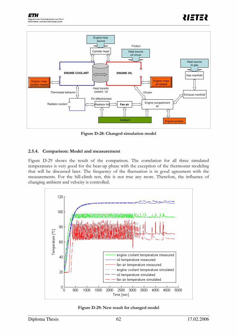
Diploma Thesis 62 17.02.2006
Figure D-28: Changed simulation model
2.5.4. Comparison: Model and measurement
Figure D-29 shows the result of the comparison. The correlation for all three simulated temperatures is very good for the heat-up phase with the exception of the thermostat modeling that will be discussed later. The frequency of the fluctuation is in good agreement with the measurements. For the hill-climb test, this is not true any more. Therefore, the influence of changing ambient and velocity is controlled.
Figure D-29: New result for changed model
Engine heat
source
Cylinder head
ENGINE COOLANT ENGINE OIL
Heat transfer
coolant / oil
Heat source
oil circuit
Friction
Radiator coolant Radiator fin Fan air
Ambient
Heat source
to gas
Gas manifold
Exhaust manifold
Engine compartment
air
Engine mass
oil heatedEngine mass
coolant heated
Oil pan
Engine surface
Thermostat behavior
Fin effectiveness

Diploma Thesis 63 17.02.2006
Influence of changing ambient and velocity
It is still not possible for the hill-climb test to fit the fan frequency compared to the heat-up. The influence of the ambient air temperature and the velocity change will therefore be investigated. Figure D-30 shows one solution for a guessing parameter set, where in the first plot, the ambient temperature is equal to the measured temperature in the rollerbench. The other three plots show the influence of changing the ambient temperature to a constant value over the whole cycle. It can be seen that for temperatures above 21°C, the fan will stay in for the whole hill-climb test. Below 20°C, the cycling frequency is increasing like the measurements have shown.
Figure D-30: Real ambient air temperature, constant ambient at 19°C, constant ambient at 20°C and constant ambient at 21°C
The reason for the change in frequency over the hill-climb test is only due the change of the velocity. It can be seen in Figure D-31 that for a constant velocity, the cycling will be periodic in the second stage.

Diploma Thesis 64 17.02.2006
Figure D-31: Simulation of a constant velocity
This result shows the importance of an accurate velocity measurement for the hill-climb test. Since the calculated acceleration comes out of an averaged velocity measurement over 10 seconds, the information about sudden changes in velocity will get lost. Furthermore, the result shows that the real behavior of the cycling cannot be modeled properly, because the engine coolant temperature shows that there is a steady increase of heat going into the coolant (or a steady decrease of heat rejection out of the coolant) in the hill-climb test. This behavior has been detected as well for the measurements at different ambient temperatures. For temperatures below 20°C, the cycling frequency is also decreased due to additional heat input. For temperatures above 20°C, the fan starts holding and after the first pull-down of the coolant, the temperature is increasing slowly but steadily.
Figure D-32: Coolant temperature increase for the hill-climb test
Standard test cycle at 28°C, transition from heat-up to hill-climb test
92
93
94
95
96
97
98
16:26:24 16:33:36 16:40:48 16:48:00 16:55:12 17:02:24
Engine coolant out

Diploma Thesis 65 17.02.2006
The influence of the ambient temperature to the cooling system is therefore very important. Compared to the 16°C measurement, an increase of 4°C will raise the fan activation by 24% and an increase of 8°C will raise it by 32%. The 20°C measurement is an intermediate state between the fan holding at 24°C and the constant cycling at 16°C. Radiator effectiveness versus fin effectiveness
The measured radiator effectiveness is shown in Figure C-16. The radiator effectiveness coming out of the simulation differs from the measured one because it is based on a mean radiator temperature. The fin efficiency, on the other hand, is binary and depends on the fan state and the heat transfer correlation coefficients. For the heat-up phase, the efficiency is cycling between two values as we can see in the measurement. For the hill-climb test, the behavior does not correspond any more to the measured data. That is one of the reasons why the absolute values of the fan air temperature are wrong in the second phase.
Figure D-33: Fin effectiveness versus radiator effectiveness during simulation
This behavior shows that a transition of the coolant flow has to take place. The Reynolds number is therefore calculated for the channel flow in the radiator.
Radiator data: Number of channels: ≈ 36 Width of one channel: ≈ 2 cm Height of one channel: ≈ 1 mm Mass flow at 1750rpm: ≈ 2573 kg/h Mass flow at 2750rpm: ≈ 4162 kg/h
mmhw
hw
P
ADh 9.1
24≈
+
⋅⋅=
⋅=
ρρ ⋅⋅=
⋅=
hw
m
A
mu
&&

Diploma Thesis 66 17.02.2006
The dynamic viscosity of a monoethylene glycol/water mixture (52/48) is µ=0.72·10-3 Ns/m2, the density ρ=1032 kg/m3, [4].
µ
ρ hDu ⋅⋅=Re
The Reynolds numbers become 2626 and 4248 for the heat-up phase and the hill-climb test, respectively. The coolant flow is normally laminar when the Reynolds number is below about 2100. In the range of Reynolds numbers between 2100 and 4000, the coolant flow is transitional. At a Reynolds number of about 4000 the coolant flow becomes fully turbulent, [2]. Nusselt correlations used so far for the coolant flow will therefore not be valid for the lower engine speed regime where the flow is still in the transitional regime. Nusselt correlations have to be adjusted depending on Reynolds number with the following relationships, [XVIII].
3
2
PrRe04.01
PrRe0668.0
66.3
⋅⋅⋅+
⋅⋅⋅+=
Y
D
Y
D
Nu
h
h
laminar (Eq. 29)
4.08.0 PrRe023.0 ⋅⋅=Nu , 0.5 < Pr <120 and Re >4000 turbulent (Eq. 30)
( ) ( )
+⋅−⋅⋅−⋅=
89.0
3.08.0 18.0Pr8.1230Re0235.0Y
DNu h transitional (Eq. 31)
2.5.5. Investigation on different parts of the test
The test drive cycle has been divided into the main three parts to investigate them separately. The first part is the warm-up phase of the engine until the engine coolant reaches the operating temperature. The second part is the heat-up phase at 80 kph in 5th gear and the third part is the hill-climb phase at 25 kph in 1st gear. Furthermore, it has been concentrated on the driving parameters in the cooling system, the engine coolant and the engine oil temperature.

Diploma Thesis 67 17.02.2006
Figure D-34: Temperature pattern of engine coolant and oil
Figure D-34 shows that the amplitude and frequency of the simulated temperatures correlate very well with the measured data. Nevertheless, a set of guessing parameters describing the total test cannot be found.
2.5.6. Dissipated heat to coolant and exhaust gas
Figure D-16 has shown the engine speed dependency of dissipated heat to useful power for an engine measurement at 20% of maximum power. This behavior of dissipated heat changes considerably as the power percentage is increased. Figure D-35 shows the influence of a change in power for the engine speed at heat-up and hill-climb phase.
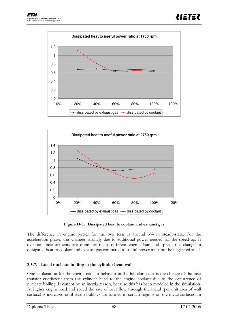
Diploma Thesis 68 17.02.2006
Figure D-35: Dissipated heat to coolant and exhaust gas
The difference in engine power for the two tests is around 3% in steady-state. For the acceleration phase, this changes strongly due to additional power needed for the speed-up. If dynamic measurements are done for many different engine load and speed, the change in dissipated heat to coolant and exhaust gas compared to useful power must not be neglected at all.
2.5.7. Local nucleate boiling at the cylinder head wall
One explanation for the engine coolant behavior in the hill-climb test is the change of the heat transfer coefficient from the cylinder head to the engine coolant due to the occurrence of nucleate boiling. It cannot be an inertia reason, because this has been modeled in the simulation. At higher engine load and speed the rate of heat flow through the metal (per unit area of wall surface) is increased until steam bubbles are formed in certain regions on the metal surfaces. In
Dissipated heat to useful power ratio at 1750 rpm
0
0.2
0.4
0.6
0.8
1
1.2
0% 20% 40% 60% 80% 100% 120%
dissipated by exhaust gas dissipated by coolant
Dissipated heat to useful power ratio at 2750 rpm
0
0.2
0.4
0.6
0.8
1
1.2
1.4
0% 20% 40% 60% 80% 100% 120%
dissipated by exhaust gas dissipated by coolant

Diploma Thesis 69 17.02.2006
this phase, large number of bubbles form on the hot surfaces and travel through the bulk of the coolant to emerge at the free surface of the filler tank. This results in an increased agitation or movement of liquid so that heat transfer is considerably improved. There is a lot of research going on in the automotive branch concerning the control of nucleate boiling. The goal is to regulate pump speed according to the instantaneous heat rejection and therefore to improve the overall efficiency. The temperature difference between the local wall temperature Tw and the saturation temperature of the coolant Tsat will define the character of the boiling process. [XVII] shows that for a 50/50 ethylene glycol/water mixture, nucleate boiling occurs for superheat temperatures between 5°C to 30°C. Below this temperature, the heat transfer is convection dominant and for higher superheat temperatures, transition and film boiling will be dominant. For automotive applications, film boiling will result in engine damage and must be avoided completely. Figure D-36 shows a qualitative plot for the different regimes of convection and boiling as a function of the superheat temperature.
Figure D-36: Qualitative plot for convection and boiling regimes
The saturation temperature itself is strongly depending on the local pressure and the mixing ratio of the coolant. Figure D-37 show these different dependencies.
Figure D-37: Boiling temperature in dependency on overpressure and coolant mixing ratio
Boiling point of ethylene glycol by changing pressure
100
105
110
115
120
125
130
135
140
145
150
0 0.2 0.4 0.6 0.8 1 1.2 1.4 1.6
overpressure [bar]
bo
ilin
g t
em
pera
ture
[°C
]

Diploma Thesis 70 17.02.2006
The strong dependency on coolant mixing ratio, local pressure, coolant mass flow and local cylinder head wall temperature makes the boiling behavior impossible to model in 1-D. Exact mass flow rates, local pressures and cylinder head geometry beside additional combustion details have to be known to take into account the nucleate boiling that might occur locally and change the heat transfer to the engine coolant immediately. Furthermore, the nucleate boiling would only occur in small “hot spot” regions of the cylinder head and would never cover the total wall surface. A combination of forced convection and nucleate boiling has to be considered. Literature research has shown that only with extensive measurements in the cylinder head region statements can be done whether nucleate boiling is existent or not. Nevertheless, the existence of nucleate boiling for high loads and low coolant mass flow as well as low local pressure has been confirmed several times.
2.5.8. Investigation on a set of guessing parameters
It has been investigated if a set of guessing parameters optimized for 20°C for the heat-up phase will also represent the cooling behavior for ambient temperatures at 12°C, 16°C, 24°C and 28°C. The comparison between the simulation and the measurement in Figure D-38 shows that the cycling frequency is changing and following the measurement data. For ambient temperatures above 20°C, the simulated frequency is too low while for temperatures below 20°C it is too high.

Diploma Thesis 71 17.02.2006
Figure D-38: Comparison of simulation and measurement for different ambient air temperatures
The general behavior of the cycling can be modeled, the exact shape of the curves after the transition to the hill-climb test cannot. These results show that the influence of the ambient change in the model is stronger than it is in reality. The coupling of the engine coolant to the ambient temperature goes over the two nodes radiator coolant and fin. Therefore, the exact heat transfer calculation in the radiator fin region is error-prone for the second test. The effects of the non-linear airflow distribution at the radiator position are important when different incoming flows are simulated. For the ambient air change investigation, the blower airspeed has always been held constant and different airflow distributions will only occur due to the fan activation. An activity of the high-speed fan has never been detected at all. Therefore, the non-linear heat transfer behavior cannot be the reason for the occurred problems.
2.5.9. Engine compartment heat-up explanation
Beside a model improvement in the heat exchanger region, the engine compartment heat-up has to be investigated in more detail. The slow transient warm-up of all the components within the engine compartment and the adjacent parts might be responsible for the changing fan cycling behavior for the hill-climb test. The engine block node could therefore be split in an average block temperature and in an average engine surface temperature. Convective and radiative heat transfer will then be formulated at the node of the surface node.

Diploma Thesis 72 17.02.2006
E. Conclusion
Within this report, it has been investigated if it is possible to predict underhood temperatures with the help of a simplified 1-D thermal model based on test data using an evolutionary algorithm. It has been shown that for a constant drive without changing engine speed or load, simulated underhood temperatures for the heat-up phase correlate very well with the measured data. The transient progression of the engine coolant, engine oil and fan air outlet temperature are assumed to characterize the cooling system. A small time delay for the fan activation has been detected; this is because of the linear ramp function used in the thermostat model. Taking into account the hysteresis of the thermostat, this time delay can be avoided. For the simulation of a standard hill-climb test, this is not of great importance, but will become relevant for stop-and-go measurements. The coupling between the 1-D Simulink model and the evolutionary algorithm has worked well and the model could be extended with the correlation results of the algorithm. For that purpose, the Simulink-model and the Matlab parameter function have been compiled, using the rapid simulation target option of the real-time workshop as well as the standard Matlab mcc compiler. To get the possibility of feeding the algorithm with changing parameters without repeating the compilation, all guessing parameters have been defined as global tunable parameters in the 1-D thermal model. The objective value of the comparison between the simulated and the measured temperature curves is defined within the evolutionary algorithm. For the 1-D model application, the evolutionary algorithm is used as a black box tool to find a set of guessing parameters describing the dynamic system. The 1-D model showed weaknesses regarding a transition to a different driving cycle when engine load and speed is changing. A fundamental different behavior has been detected for the hill-climb phase that could not be simulated with the current 1-D model. Several problems have been highlighted regarding underhood and underbody modeling. Possible reasons for the temperature behavior change in the hill-climb test have been enumerated. For the exhaust airflow calculation, the behavior of the turbocharger and intercooler is essential. Detailed information about the waste gate valve operation and the boost pressure has not been available until the end of this work. For an expansion of the model network, more data have to be included from the acquired ECU diagnostics box. The problems occurred during the underhood simulation stopped a proper investigation of the underbody region because the output parameters of the first model will be the input parameters of the second one. For an exact analysis of the influences of environmental and driving changes, the existing model has to be improved and expanded.

Diploma Thesis 73 17.02.2006
F. Outlook
The problem of effects of environmental and driving changes on underhood and underbody regions of a vehicle is ongoing. To achieve the long-term goal for a comparison between rollerbench and on-road measurements, more investigations have to follow in the future. The transition to underbody modeling awaits good correlation of input air temperatures from the model. Additionally, the mixing phenomena between the underbody and the road will be a key part of the heat transfer calculation. If the 1-D model approach using an evolutionary algorithm is pursued, certain problems have to be solved at first. The thermostat hysteresis modeling should be done to include transient driving conditions as well. Accurate geometry and flow details in the radiator area have to be incorporated to take into account the non-linearities of the heat exchanger. An additional thermal node for the engine surface temperature might be necessary for a better correlation for the overall test drive. An investigation of the appearance of nucleate boiling in the cooling jacket region is very difficult. Nevertheless, it has to be checked if the increased heat transfer rate at the hill-climb test is a consequence of the boiling or if it has other causes. If the node network of the 1-D simulation is expanded, more heat transfer connections can be implemented. The general problem is that the simplified structure might get lost and that the dynamics of the system will be hard to understand. Additionally, the inclusion of more guessing parameters will bring difficulties for the evolutionary algorithm regarding an acceptable computing time. A tradeoff has to be found between the number of guessing parameters and the amount of measurements at the vehicle. For the transition to the underbody region, more measurement data have to be included. With the ECU diagnostics box, the behavior of the turbocharger, the intercooler, the exhaust gas recirculation etc. can be understood. These additional measurements will lead to a proper calculation of the exhaust gas temperature and are essential for the boundary conditions of the underbody model.

Diploma Thesis 74 17.02.2006
G. Appendix
10. Heat capacity calculation of exhaust air
For the exhaust gas temperature calculation, the effective heat capacity value has to be known. This value is changing considerably with temperature, so that the dependency must not be neglected. The exhaust air is assumed to be an ideal gas. The gas constant R is constant and specific heat capacity at constant pressure cp and volume cv will only be a function of temperature T.
)(TfdT
dhc p == )(Tg
dT
ducv ==
vp ccR −=
Kkg
JR gas exhaust
⋅≈ 6.286
In [7], the behavior of R
c p as a function of temperature T can be consulted. These material
properties can be used in good approximation for diesel as well as for Otto processes because the thermodynamic properties of the exhaust gases are changing slightly even for different fuel compositions. The derivation comes out of the combustion formula:
22222188 74.539874.535.12 NOHCONOHC ++↔++
and
222223416 35.105171635.1055.24 NOHCONOHC ++↔++ ,
respectively. For an exhaust gas temperature of 800 K, we will get an approximate exhaust gas heat capacity of 1190 J/kgK.

Diploma Thesis 75 17.02.2006
comparison of temperatures / not normalized
body tunnel 1 / cut / stretchedbasline01_Test01
basline02_Test02
basline03_Test07
0
10
20
30
40
50
60
70
80
90
100
00:00:00 00:02:53 00:05:46 00:08:38 00:11:31 00:14:24 00:17:17 00:20:10 00:23:02 00:25:55 00:28:48
Time
Tem
pera
ture
in
°C
basline01_Test01 6[°C] body tunnel1 basline01_Test01 26[°C] air ambient basline02_Test02 6[°C] body tunnel1
basline02_Test02 26[°C] air ambient basline03_Test07 6[°C] body tunnel1 basline03_Test07 26[°C] air ambient
11. Measured on-road temperatures for the underbody region
comparison of temperatures / not normalized
body tunnel 2 / cut / stretchedbasline01_Test01
basline02_Test02
basline03_Test07
0
10
20
30
40
50
60
70
80
00:00:00 00:02:53 00:05:46 00:08:38 00:11:31 00:14:24 00:17:17 00:20:10 00:23:02 00:25:55 00:28:48
Time
Te
mp
era
ture
in
°C
basline01_Test01 7[°C] body tunnel2 basline01_Test01 26[°C] air ambient basline02_Test02 7[°C] body tunnel2
basline02_Test02 26[°C] air ambient basline03_Test07 7[°C] body tunnel2 basline03_Test07 26[°C] air ambient
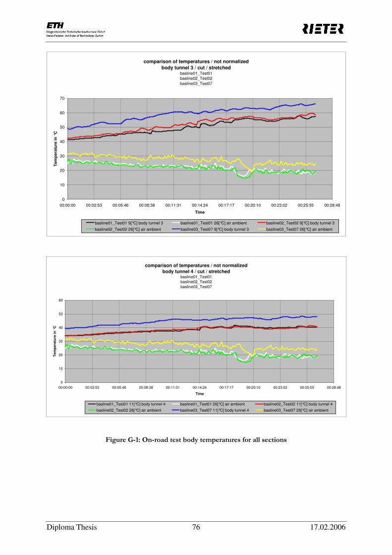
Diploma Thesis 76 17.02.2006
Figure G-1: On-road test body temperatures for all sections
comparison of temperatures / not normalized
body tunnel 3 / cut / stretchedbasline01_Test01
basline02_Test02
basline03_Test07
0
10
20
30
40
50
60
70
00:00:00 00:02:53 00:05:46 00:08:38 00:11:31 00:14:24 00:17:17 00:20:10 00:23:02 00:25:55 00:28:48
Time
Te
mp
era
ture
in
°C
basline01_Test01 9[°C] body tunnel 3 basline01_Test01 26[°C] air ambient basline02_Test02 9[°C] body tunnel 3
basline02_Test02 26[°C] air ambient basline03_Test07 9[°C] body tunnel 3 basline03_Test07 26[°C] air ambient
comparison of temperatures / not normalized
body tunnel 4 / cut / stretchedbasline01_Test01
basline02_Test02
basline03_Test07
0
10
20
30
40
50
60
00:00:00 00:02:53 00:05:46 00:08:38 00:11:31 00:14:24 00:17:17 00:20:10 00:23:02 00:25:55 00:28:48
Time
Tem
pera
ture
in
°C
basline01_Test01 11[°C] body tunnel 4 basline01_Test01 26[°C] air ambient basline02_Test02 11[°C] body tunnel 4
basline02_Test02 26[°C] air ambient basline03_Test07 11[°C] body tunnel 4 basline03_Test07 26[°C] air ambient

Diploma Thesis 77 17.02.2006
comparison of temperatures / not normalized
heatshield tunnel 1 / cut / stretchedbasline01_Test01
basline02_Test02
basline03_Test07
0
20
40
60
80
100
120
00:00:00 00:02:53 00:05:46 00:08:38 00:11:31 00:14:24 00:17:17 00:20:10 00:23:02 00:25:55 00:28:48
Time
Te
mp
era
ture
in
°C
basline01_Test01 20[°C] HS1 basline01_Test01 26[°C] air ambient basline02_Test02 20[°C] HS1
basline02_Test02 26[°C] air ambient basline03_Test07 20[°C] HS1 basline03_Test07 26[°C] air ambient
comparison of temperatures / not normalized
heatshield tunnel 2 / cut / stretchedbasline01_Test01
basline02_Test02
basline03_Test07
0
10
20
30
40
50
60
70
80
90
00:00:00 00:02:53 00:05:46 00:08:38 00:11:31 00:14:24 00:17:17 00:20:10 00:23:02 00:25:55 00:28:48
Time
Tem
pera
ture
in
°C
basline01_Test01 21[°C] HS2 basline01_Test01 26[°C] air ambient basline02_Test02 21[°C] HS2
basline02_Test02 26[°C] air ambient basline03_Test07 21[°C] HS2 basline03_Test07 26[°C] air ambient

Diploma Thesis 78 17.02.2006
Figure G-2: On-road test heatshield temperatures for all sections
comparison of temperatures / not normalized
heatshield tunnel 3 / cut / stretchedbasline01_Test01
basline02_Test02
basline03_Test07
0
10
20
30
40
50
60
70
80
90
00:00:00 00:02:53 00:05:46 00:08:38 00:11:31 00:14:24 00:17:17 00:20:10 00:23:02 00:25:55 00:28:48
Time
Tem
pera
ture
in
°C
basline01_Test01 22[°C] HS3 basline01_Test01 26[°C] air ambient basline02_Test02 22[°C] HS3
basline02_Test02 26[°C] air ambient basline03_Test07 22[°C] HS3 basline03_Test07 26[°C] air ambient
comparison of temperatures / not normalized
heatshield tunnel 4 / cut / stretchedbasline01_Test01
basline02_Test02
basline03_Test07
0
10
20
30
40
50
60
70
00:00:00 00:02:53 00:05:46 00:08:38 00:11:31 00:14:24 00:17:17 00:20:10 00:23:02 00:25:55 00:28:48
Time
Te
mp
era
ture
in
°C
basline01_Test01 23[°C] HS4 basline01_Test01 26[°C] air ambient basline02_Test02 23[°C] HS4
basline02_Test02 26[°C] air ambient basline03_Test07 23[°C] HS4 basline03_Test07 26[°C] air ambient
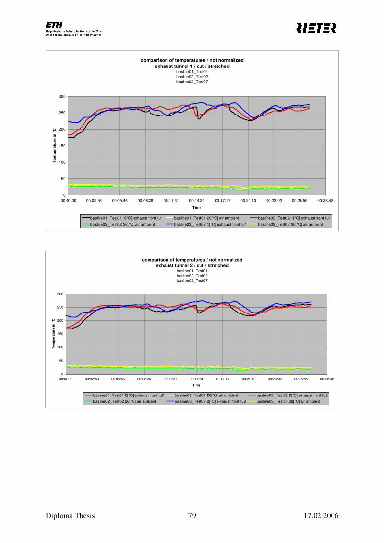
Diploma Thesis 79 17.02.2006
comparison of temperatures / not normalized
exhaust tunnel 1 / cut / stretchedbasline01_Test01
basline02_Test02
basline03_Test07
0
50
100
150
200
250
300
00:00:00 00:02:53 00:05:46 00:08:38 00:11:31 00:14:24 00:17:17 00:20:10 00:23:02 00:25:55 00:28:48
Time
Te
mp
era
ture
in
°C
basline01_Test01 1[°C] exhaust front tu1 basline01_Test01 26[°C] air ambient basline02_Test02 1[°C] exhaust front tu1
basline02_Test02 26[°C] air ambient basline03_Test07 1[°C] exhaust front tu1 basline03_Test07 26[°C] air ambient
comparison of temperatures / not normalized
exhaust tunnel 2 / cut / stretchedbasline01_Test01
basline02_Test02
basline03_Test07
0
50
100
150
200
250
300
00:00:00 00:02:53 00:05:46 00:08:38 00:11:31 00:14:24 00:17:17 00:20:10 00:23:02 00:25:55 00:28:48
Time
Tem
pera
ture
in
°C
basline01_Test01 2[°C] exhaust front tu2 basline01_Test01 26[°C] air ambient basline02_Test02 2[°C] exhaust front tu2
basline02_Test02 26[°C] air ambient basline03_Test07 2[°C] exhaust front tu2 basline03_Test07 26[°C] air ambient

Diploma Thesis 80 17.02.2006
Figure G-3: On-road test exhaust temperatures for all sections
comparison of temperatures / not normalized
exhaust tunnel 3 / cut / stretchedbasline01_Test01
basline02_Test02
basline03_Test07
0
50
100
150
200
250
300
00:00:00 00:02:53 00:05:46 00:08:38 00:11:31 00:14:24 00:17:17 00:20:10 00:23:02 00:25:55 00:28:48
Time
Te
mp
era
ture
in
°C
basline01_Test01 4[°C] exhaust tunnel3 basline01_Test01 26[°C] air ambient basline02_Test02 4[°C] exhaust tunnel3
basline02_Test02 26[°C] air ambient basline03_Test07 4[°C] exhaust tunnel3 basline03_Test07 26[°C] air ambient
comparison of temperatures / not normalized
exhaust tunnel 4 / cut / stretchedbasline01_Test01
basline02_Test02
basline03_Test07
0
50
100
150
200
250
300
00:00:00 00:02:53 00:05:46 00:08:38 00:11:31 00:14:24 00:17:17 00:20:10 00:23:02 00:25:55 00:28:48
Time
Te
mp
era
ture
in
°C
basline01_Test01 5[°C] exhaust tunnel4 basline01_Test01 26[°C] air ambient basline02_Test02 5[°C] exhaust tunnel4
basline02_Test02 26[°C] air ambient basline03_Test07 5[°C] exhaust tunnel4 basline03_Test07 26[°C] air ambient

Diploma Thesis 81 17.02.2006
12. Matlab-model
Matlabmodel.m
% -------------------------------------------------------------------------
% Matlab-model:
% -------------------------------------------------------------------------
clc;
clear all;
close all;
% Choose time-step for the calculation
time_step_sec = 5; %(0.1,1,5 or 10 seconds) CHANGEABLE
% -------------------------------------------------------------------------
% Guessing parameters:
% -------------------------------------------------------------------------
% These parameters are not know a-priori. Because of measurements and/or
% estimations, the ranges of the parameters can be given.
% cooling system
coolant_mass = 5; % [4,7]
effective_engine_mass = 80; % [10,300]
coolant_inertial_balance = 0.7; % [0,1]
coolant_heat_balance = 0.8; % [0,1]
radiator_airflow1 = 1.3; % [0.5,6.0]
delta_radiator_airflow = 0; % [0,2], for rollerbench test: =0
ram_air_coeff = 0.002; % [0,0.005]
oil2water_conductance = 0.22; % [0,1]
exhaust_underbody_escaping = 1.15; % [0.2,1.5]
exhaust_underhood = 0.08; % [0.01,0.1]
coolant_side = 1.0; % [0.5,2.0]
underhood_cooling_factor = 80; % [0,200]
radiator_efficiency = 0.7; % [0.5,1.0]
% -------------------------------------------------------------------------
% Input variables:
% -------------------------------------------------------------------------
% These parameters can either be consulted at a vehicle technical data
% sheet and/or measured directly at the investigated car.
% vehicle data
area = 1.82;
drag_coeff = 0.32;
rolling_resist = 0.0124;
train_mass = 1800;
% engine type and gear ratios
engine_size = 1.91;
cylinders = 8;
gearratio1 = 3.8;
gearratio2 = 2.24;
gearratio3 = 1.36;
gearratio4 = 0.97;
gearratio5 = 0.76;
axis = 3.35;
tire1 = 195;
tire2 = 60;
rim_diameter = 15;
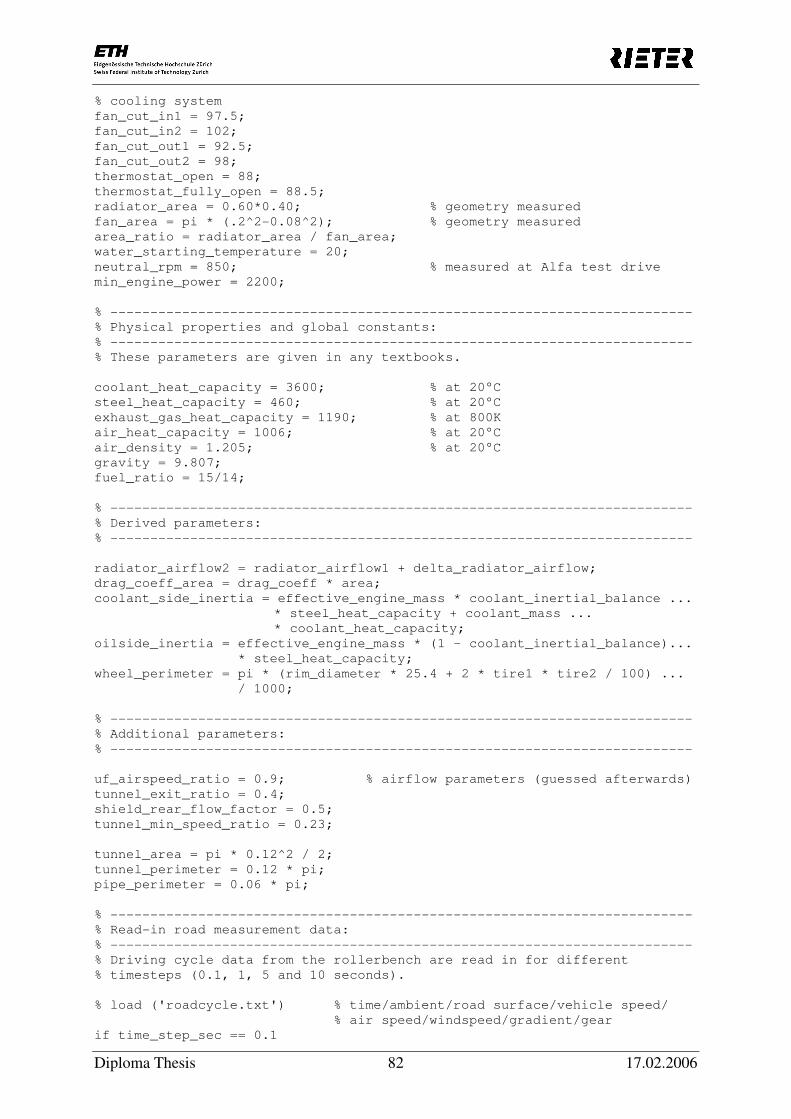
Diploma Thesis 82 17.02.2006
% cooling system
fan_cut_in1 = 97.5;
fan_cut_in2 = 102;
fan_cut_out1 = 92.5;
fan_cut_out2 = 98;
thermostat_open = 88;
thermostat_fully_open = 88.5;
radiator_area = 0.60*0.40; % geometry measured
fan_area = pi * (.2^2-0.08^2); % geometry measured
area_ratio = radiator_area / fan_area;
water_starting_temperature = 20;
neutral_rpm = 850; % measured at Alfa test drive
min_engine_power = 2200;
% -------------------------------------------------------------------------
% Physical properties and global constants:
% -------------------------------------------------------------------------
% These parameters are given in any textbooks.
coolant_heat_capacity = 3600; % at 20°C
steel_heat_capacity = 460; % at 20°C
exhaust_gas_heat_capacity = 1190; % at 800K
air_heat_capacity = 1006; % at 20°C
air_density = 1.205; % at 20°C
gravity = 9.807;
fuel_ratio = 15/14;
% -------------------------------------------------------------------------
% Derived parameters:
% -------------------------------------------------------------------------
radiator_airflow2 = radiator_airflow1 + delta_radiator_airflow;
drag_coeff_area = drag_coeff * area;
coolant_side_inertia = effective_engine_mass * coolant_inertial_balance ...
* steel_heat_capacity + coolant_mass ...
* coolant_heat_capacity;
oilside_inertia = effective_engine_mass * (1 - coolant_inertial_balance)...
* steel_heat_capacity;
wheel_perimeter = pi * (rim_diameter * 25.4 + 2 * tire1 * tire2 / 100) ...
/ 1000;
% -------------------------------------------------------------------------
% Additional parameters:
% -------------------------------------------------------------------------
uf_airspeed_ratio = 0.9; % airflow parameters (guessed afterwards)
tunnel_exit_ratio = 0.4;
shield_rear_flow_factor = 0.5;
tunnel_min_speed_ratio = 0.23;
tunnel_area = pi * 0.12^2 / 2;
tunnel_perimeter = 0.12 * pi;
pipe_perimeter = 0.06 * pi;
% -------------------------------------------------------------------------
% Read-in road measurement data:
% -------------------------------------------------------------------------
% Driving cycle data from the rollerbench are read in for different
% timesteps (0.1, 1, 5 and 10 seconds).
% load ('roadcycle.txt') % time/ambient/road surface/vehicle speed/
% air speed/windspeed/gradient/gear
if time_step_sec == 0.1

Diploma Thesis 83 17.02.2006
roadcycle = load ('rollerbench01seconds.txt');
else if time_step_sec == 1
roadcycle = load ('rollerbench1seconds.txt');
else if time_step_sec == 5
roadcycle = load ('rollerbench5seconds.txt');
else if time_step_sec == 10
roadcycle = load ('rollerbench10seconds.txt');
end
end
end
end
data = zeros(roadcycle(1),30);
load ('roadmeasurement.txt'); % measurement data from on-road tests
% -------------------------------------------------------------------------
% Load heat transfer data:
% -------------------------------------------------------------------------
% This data comes out of the heattransfer.m program and will deliver a
% table with the velocity speeds vs. heat transfer coefficients calculated
% with the the flat plate assumption
load('htdata.mat');
% includes htcoeff
% -------------------------------------------------------------------------
% Calculation:
% -------------------------------------------------------------------------
% In this section, all the parameters are calculated and optimized by
% comparing them to the measurement data. Finally, the output variables
% will be the input variables for the simulation of the underbody.
% engine speed (data 1) / engine load (data 2) / engine power (data 3)
for i=1:size(roadcycle,1)
if roadcycle(i,8) == 0
data(i,1) = neutral_rpm;
data(i,2) = 0;
data(i,3) = min_engine_power;
elseif roadcycle(i,8) == 1
data(i,1) = roadcycle(i,4)/3.6/wheel_perimeter*60*(axis*gearratio1);
elseif roadcycle(i,8) == 2
data(i,1) = roadcycle(i,4)/3.6/wheel_perimeter*60*(axis*gearratio2);
elseif roadcycle(i,8) == 3
data(i,1) = roadcycle(i,4)/3.6/wheel_perimeter*60*(axis*gearratio3);
elseif roadcycle(i,8) == 4
data(i,1) = roadcycle(i,4)/3.6/wheel_perimeter*60*(axis*gearratio4);
elseif roadcycle(i,8) == 5
data(i,1) = roadcycle(i,4)/3.6/wheel_perimeter*60*(axis*gearratio5);
end
end
for i=1:size(roadcycle,1)
if roadcycle(i,8) ~= 0
data(i,2) = (roadcycle(i,4)/3.6)^2*(air_density/2)*drag_coeff_area...
+gravity*train_mass*rolling_resist+gravity*0.01...
*train_mass*roadcycle(i,7);
data(i,3) = max(min_engine_power,data(i,2)*roadcycle(i,4)/3.6);
end
end
% initial entries
data(1,4) = (roadcycle(1,5)/3.6)^2*ram_air_coeff;

Diploma Thesis 84 17.02.2006
data(1,5) = 0;
data(1,6) = water_starting_temperature;
data(1,8) = 0;
data(1,9) = 0;
data(1,10) = roadcycle(1,2);
data(1,11) = 0;
data(1,12) = data(1,6);
data(1,14) = data(1,6);
data(1,7) = (data(1,12)-data(1,6))*oil2water_conductance;
data(1,13) = data(1,3)*exhaust_underhood;
data(1,15) = tunnel_exit_ratio*radiator_area*data(1,4)*1000*60;
data(1,16) = engine_size/2*data(1,1);
data(1,17) = data(1,16)/1000/60/air_density*fuel_ratio;
data(1,18) = data(1,3)*exhaust_underbody_escaping/(data(1,17)...
*exhaust_gas_heat_capacity)+roadcycle(1,2);
data(1,19) = max(data(1,15)/1000/60/tunnel_area*3.6,roadcycle(1,4)...
*tunnel_min_speed_ratio);
data(1,20) = roadcycle(1,4)*uf_airspeed_ratio;
% radiator airflow / cooling power / water temperature / oil to water /
% fan demand / fan state / fan exit air / engine surface / air temperature/
% radiation within EC / engine compartment exit / tunnel flow / exhaust
% gasflow / exhaust gas temperature / tunnel speed / floor speed
for i=2:size(roadcycle,1)
% radiator airflow (data 4)
if data(i-1,9) < 1
data(i,4) = (roadcycle(i,5)/3.6)^2*ram_air_coeff;
elseif data(i-1,9) == 1
data(i,4) = max(data(i-1,4),radiator_airflow1);
else
data(i,4) = max(data(i-1,4),radiator_airflow2);
end
% cooling conductance (data 5)
if data(i-1,6) < thermostat_fully_open
if data(i-1,6) > thermostat_open
data(i,5) = data(i,4)*radiator_area*radiator_efficiency...
*air_heat_capacity*air_density;
else
data(i,5) = 0;
end
else
data(i,5) = data(i,4)*radiator_area*radiator_efficiency...
*air_heat_capacity*air_density;
end
% water temperature (data 6)
data(i,6) = (roadcycle(i,1)-roadcycle(i-1,1))*((data(i,3)+data(i-1,3))
*coolant_heat_balance*coolant_side/2-data(i,5)...
*(data(i-1,6)-roadcycle(i-1,2))+data(i-1,7))*60 ...
/coolant_side_inertia+data(i-1,6);
% oil to water (data 7)
data(i,7) = (data(i-1,12)-data(i-1,6))*oil2water_conductance*data(i,1);
% fan demand (data 8)
if data(i,6) > fan_cut_in1
if data(i,6) > fan_cut_in2
data(i,8) = 2;
else
data(i,8) = 1;
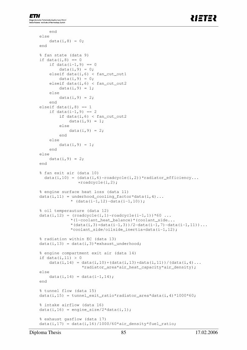
Diploma Thesis 85 17.02.2006
end
else
data(i,8) = 0;
end
% fan state (data 9)
if data(i,8) == 0
if data(i-1,9) == 0
data(i,9) = 0;
elseif data(i,6) < fan_cut_out1
data(i,9) = 0;
elseif data(i,6) < fan_cut_out2
data(i,9) = 1;
else
data(i,9) = 2;
end
elseif data(i,8) == 1
if data(i-1,9) == 2
if data(i,6) < fan_cut_out2
data(i,9) = 1;
else
data(i,9) = 2;
end
else
data(i,9) = 1;
end
else
data(i,9) = 2;
end
% fan exit air (data 10)
data(i,10) = (data(i,6)-roadcycle(i,2))*radiator_efficiency...
+roadcycle(i,2);
% engine surface heat loss (data 11)
data(i,11) = underhood_cooling_factor*data(i,4)...
* (data(i-1,12)-data(i-1,10));
% oil temperauture (data 12)
data(i,12) = (roadcycle(i,1)-roadcycle(i-1,1))*60 ...
*(1-coolant_heat_balance)*(coolant_side...
*(data(i,3)+data(i-1,3))/2-data(i-1,7)-data(i-1,11))...
*coolant_side/oilside_inertia+data(i-1,12);
% radiation within EC (data 13)
data(i,13) = data(i,3)*exhaust_underhood;
% engine compartment exit air (data 14)
if data(i,11) > 0
data(i,14) = data(i,10)+(data(i,13)+data(i,11))/(data(i,4)...
*radiator_area*air_heat_capacity*air_density);
else
data(i,14) = data(i-1,14);
end
% tunnel flow (data 15)
data(i,15) = tunnel_exit_ratio*radiator_area*data(i,4)*1000*60;
% intake airflow (data 16)
data(i,16) = engine_size/2*data(i,1);
% exhaust gasflow (data 17)
data(i,17) = data(i,16)/1000/60*air_density*fuel_ratio;

Diploma Thesis 86 17.02.2006
% exhaust gas temperature (data 18)
data(i,18) = data(i,3)*exhaust_underbody_escaping/(data(i,17)...
*exhaust_gas_heat_capacity)+roadcycle(i,2);
% tunnel speed (data 19)
data(i,19) = max(data(i,15)/1000/60/tunnel_area*3.6,roadcycle(i,4)...
*tunnel_min_speed_ratio);
% floor speed (data 20)
data(i,20) = roadcycle(i,4)*uf_airspeed_ratio;
end
for i=1:size(roadcycle,1)
% sector 1 floor h (data 21)
data(i,21) = interp1(htcoeff(:,1),htcoeff(:,2),data(i,20))/2;
% sector 2 floor h (data 22)
data(i,22) = interp1(htcoeff(:,1),htcoeff(:,3),data(i,20))/2;
% sector 3 floor h (data 23)
data(i,23) = interp1(htcoeff(:,1),htcoeff(:,4),data(i,20))/2;
% sector 4 floor h (data 24)
data(i,24) = interp1(htcoeff(:,1),htcoeff(:,5),data(i,20))/2;
% sector 5 floor h (data 25)
data(i,25) = interp1(htcoeff(:,1),htcoeff(:,6),data(i,20))/2;
% sector 1 tunnel h (data 26)
data(i,26) = interp1(htcoeff(:,1),htcoeff(:,2),data(i,19))/2;
% sector 2 tunnel h (data 27)
data(i,27) = interp1(htcoeff(:,1),htcoeff(:,3),data(i,19)); % geometry
% sector 3 tunnel h (data 28)
data(i,28) = interp1(htcoeff(:,1),htcoeff(:,4),data(i,19))/2;
% sector 4 tunnel h (data 29)
data(i,29) = interp1(htcoeff(:,1),htcoeff(:,5),data(i,19))/2;
% sector 5 tunnel h (data 30)
data(i,30) = interp1(htcoeff(:,1),htcoeff(:,6),data(i,19))/2;
end
% -------------------------------------------------------------------------
% Graphs:
% -------------------------------------------------------------------------
% Temperature characteristics are shown here for the exhaust, water, oil
% and fan exit air temperature
figure;
hold on;
plot(roadcycle(:,1),data(:,6),'b');
plot(roadcycle(:,1),data(:,10),'g'),;
plot(roadcycle(:,1),data(:,12),'r');
% plot(roadcycle(:,1),data(:,18),'c');
plot(roadmeasurement(:,5),roadmeasurement(:,1),'m');
plot(roadmeasurement(:,5),roadmeasurement(:,2),'y');
plot(roadmeasurement(:,5),roadmeasurement(:,3),'k');
% plot(roadmeasurement(:,5),roadmeasurement(:,4),'b');
% 'exit gas temperature','exit gas temperature measured'
legend('water temperature','fan exit air','oil temperature'...

Diploma Thesis 87 17.02.2006
,'water temperature measured'...
,'fan exit air measured','oil temperature measured')
hold off;
heattransfer.m
% -------------------------------------------------------------------------
% heat transfer coefficient calculation:
% -------------------------------------------------------------------------
air_density = 1.2;
air_viscosity = 0.0000181;
air_conductivity = 0.03;
section_length = 0.5;
section_number = 5;
prandtl_number = 0.72;
turbulent_prandtl_number = 0.85;
transition_reynolds_number = 500000;
htcoeff = zeros(20,section_number+1);
step = 1;
for i=10:10:200 % different vehicle speed (kph)
htcalc = zeros(section_number,9);
for j=1:section_number
htcalc(j,1) = j;
htcalc(j,2) = section_length * htcalc(j,1) * i/3.6 * air_density...
/air_viscosity;
if htcalc(j,2) > transition_reynolds_number
htcalc(j,3) = 0.037 * prandtl_number^(1/3)...
*(htcalc(j,2)^(4/5) - 23550);
else
htcalc(j,3) = 0.664 * prandtl_number^(1/3)...
*htcalc(j,2)^(1/2);
end
htcalc(j,4) = htcalc(j,3) * air_conductivity...
/(htcalc(j,1) * section_length);
htcalc(j,5) = 1 / htcalc(j,1);
if htcalc(j,1) == 1
htcalc(j,6) = htcalc(j,4);
else
htcalc(j,6) = (htcalc(j,4)-htcalc(j-1,4)*(1-htcalc(j,5)))...
/htcalc(j,5);
end
if htcalc(j,2) < transition_reynolds_number
htcalc(j,7) = 4.92 / sqrt(htcalc(j,2)) * section_length...
*htcalc(j,1);
else
htcalc(j,7) = 0.37 * section_length * htcalc(j,1) * (i/3.6...
*section_length * htcalc(j,1) * air_density...
/air_viscosity)^(-1/2);
end
if htcalc(j,2) < transition_reynolds_number
htcalc(j,8) = htcalc(j,7) / prandtl_number;
else
htcalc(j,8) = htcalc(j,7) / turbulent_prandtl_number;
end
htcalc(j,9) = htcalc(j,6) * 2;
end
htcoeff(step,1) = i;
htcoeff(step,2:6) = htcalc(:,9);
step = step + 1;
end
save htdata htcoeff;

Diploma Thesis 88 17.02.2006
13. Simulink/Matlab-model
simulation_funct.m
function simulation_funct()
% -------------------------------------------------------------------------
% CHANGE INITIAL TEMPERATURE TO AMBIENT TEMPERATURE OF MEASUREMENT
% -------------------------------------------------------------------------
% -------------------------------------------------------------------------
% CHANGE AMBIENT TEMPERATURE, VEHICLE SPEED AND ACCELERATION IN
% THE SIGNAL BUILDER OF THE SIMULINK MODEL
% Remark: The velocity logging for low speeds (v<30 kph) is not very
% accurate, it can change the values in the range of 4kph even for constant
% signal inputs. Therefore, this value is averaged over 10 seconds.
% -------------------------------------------------------------------------
if exist('input.mat')~=2
input_values={1.54,70,4,20,1.5,1.7,0.89,0.9,1.7,1.88,0.037,0.013,0.04,2.0,
0.6,0.15,0,1,3,0.56,0.62,0.3,0.5,1,0.87,0.0024,0.98,0,1};
volume_rad_coolant = input_values{1}; % [1,2]
mass_engine = input_values{2}; % [60,90]
mass_fin = input_values{3}; % [3,5]
mass_head = input_values{4}; % [10,30]
heat2gas = input_values{5}; % [0.5,3]
heat2gas2 = input_values{6}; % [0.5,3]
heat2oil = input_values{7}; % [0.5,1.5]
heat2oil2 = input_values{8}; % [0.5,1.5]
heat2head = input_values{9}; % [0.5,2]
heat2head2 = input_values{10}; % [0.5,2]
C_oil_eng_coolant = input_values{11}; % [0,0.5]
C_oil_engine = input_values{12}; % [0,0.1]
C_eng_coolant_engine = input_values{13}; % [0,0.5]
C_eng_coolant_rad_coolant = input_values{14}; % [0,10]
C_rad_coolant_fin = input_values{15}; % [0,5]
C_head_eng_coolant = input_values{16}; % [0,5]
C_head_oil = input_values{17}; % [0,0.01]
eng_conv_guess = input_values{18}; % [0,10]
oilsump_conv_guess = input_values{19}; % [0,10]
fin_conv_guess1 = input_values{20}; % [0,5]
fin_conv_guess2 = input_values{21}; % [0,1]
exhaust_conv_guess1 = input_values{22}; % [0,5]
exhaust_conv_guess2 = input_values{23}; % [0,1]
exhaust_inflow_guess = input_values{24}; % [0,10]
radiator_airflow1 = input_values{25}; % [0.2,2.0]
ram_air_coeff = input_values{26}; % [0,0.02]
max_fin_effectiveness = input_values{27}; % [0.5,1]
mixing_guess = input_values{28}; % [0,1]
rpm_exponent = input_values{29}; % [0.5,1]
disp('loading default values...')
else
load('input.mat');
disp('loading optimized values')
end
% -------------------------------------------------------------------------
% Input variables:
% -------------------------------------------------------------------------
% These parameters can either be consulted at a vehicle technical data
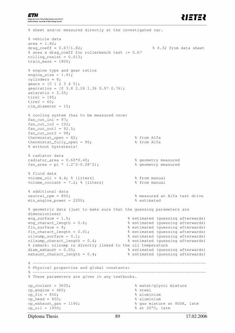
Diploma Thesis 89 17.02.2006
% sheet and/or measured directly at the investigated car.
% vehicle data
area = 1.82;
drag_coeff = 0.67/1.82; % 0.32 from data sheet
% area x drag_coeff for rollerbench test := 0.67
rolling_resist = 0.013;
train_mass = 1800;
% engine type and gear ratios
engine_size = 1.91;
cylinders = 8;
gears = [0 1 2 3 4 5];
gearratios = [0 3.8 2.24 1.36 0.97 0.76];
axisratio = 3.35;
tire1 = 195;
tire2 = 60;
rim_diameter = 15;
% cooling system (has to be measured once)
fan_cut_in1 = 97;
fan_cut_in2 = 102;
fan_cut_out1 = 92.5;
fan_cut_out2 = 98;
thermostat_open = 82; % from Alfa
thermostat_fully_open = 90; % from Alfa
% without hysteresis!
% radiator data
radiator_area = 0.60*0.40; % geometry measured
fan_area = pi * (.2^2-0.08^2); % geometry measured
% fluid data
volume_oil = 4.4; % [liters] % from manual
volume_coolant = 7.2; % [liters] % from manual
% additional data
neutral_rpm = 850; % measured at Alfa test drive
min_engine_power = 2200; % estimated
% geometric data (just to make sure that the guessing parameters are
dimensionless)
eng_surface = 1.5; % estimated (guessing afterwards)
eng_charact_length = 0.6; % estimated (guessing afterwards)
fin_surface = 8; % estimated (guessing afterwards)
fin_charact_length = 0.01; % estimated (guessing afterwards)
oilsump_surface = 0.1; % estimated (guessing afterwards)
oilsump_charact_length = 0.4; % estimated (guessing afterwards)
% remark: oilsump is directly linked to the oil temperature
diam_exhaust = 0.05; % estimated (guessing afterwards)
exhaust_charact_length = 0.4; % estimated (guessing afterwards)
% -------------------------------------------------------------------------
% Physical properties and global constants:
% -------------------------------------------------------------------------
% These parameters are given in any textbooks.
cp_coolant = 3600; % water/glycol mixture
cp_engine = 460; % steel
cp_fin = 850; % aluminium
cp_head = 850; % aluminium
cp_exhaust_gas = 1190; % gas mixture at 800K, 1atm
cp_oil = 1950; % at 20°C, 1atm

Diploma Thesis 90 17.02.2006
cp_air = 1006; % at 20°C, 1atm
density_air = 1.205; % at 20°C, 1atm
density_oil = 880; % average
density_coolant = 1040; % average
density_exhaust_gas = 0.451; % at 800K, 1atm
k_air = 0.025; % conductivity at 20°C, 1atm
k_exhaust_gas = 0.0551; % conductivity at 800K, 1atm
mu_air = 1.81e-5; % viscosity at 20°C
mu_exhaust_gas = 3.41e-5; % viscosity at 800K, 1atm
gravity = 9.807;
fuel_ratio = 15/14; % same for gasoline and diesel
prandtl_number = cp_air*mu_air/k_air; % at 20°C
% -------------------------------------------------------------------------
% Derived parameters:
% -------------------------------------------------------------------------
delta_radiator_airflow = 0; % [0,4] % FOR ROLLERBENCH TEST:= 0
radiator_airflow2 = radiator_airflow1 + delta_radiator_airflow;
drag_coeff_area = drag_coeff * area;
wheel_perimeter = pi * (rim_diameter*25.4 + 2*tire1*tire2 / 100) / 1000;
fan_area_ratio = radiator_area / fan_area;
mass_oil = volume_oil * density_oil / 1000;
mass_coolant = volume_coolant * density_coolant / 1000;
mass_rad_coolant = volume_rad_coolant * density_coolant / 1000;
mass_eng_coolant = mass_coolant - mass_rad_coolant;
% -------------------------------------------------------------------------
% Component temperatures:
% -------------------------------------------------------------------------
temp_initial = 20; % is equal to ambient temperature of measurement
% -------------------------------------------------------------------------
% Simulation / Output:
% -------------------------------------------------------------------------
% parameters used for simulink
save('parameters'); % all parameters
load('rtP.mat'); % template for required
structure
c={rtP.parameters.map.Identifier};
n=size(c,2);
d=[];for i=1:n,d=[d eval(c{i})];end
rtP.parameters.values=d;
save run.mat rtP % parameters for simulink model in required
structure form
% measured parameters
if exist('data_new.mat')~=2
load('data_new.txt');
save data data_new;
end
% simulation with simulink model
!temp_calc -p run.mat
% compiled simulink model with real-time workshop and inline parameters
% writes out all calcualted parameters in: temp_calc.mat
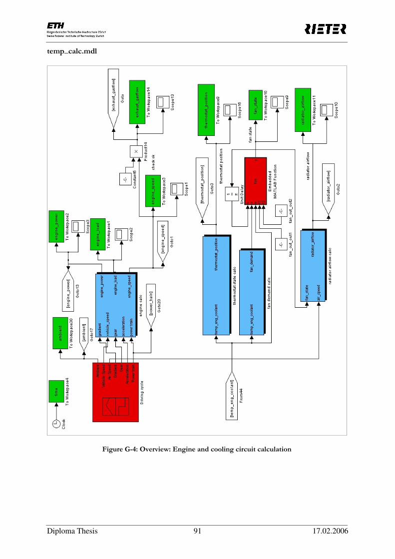
Diploma Thesis 91 17.02.2006
temp_calc.mdl
Figure G-4: Overview: Engine and cooling circuit calculation

Diploma Thesis 92 17.02.2006

Diploma Thesis 93 17.02.2006

Diploma Thesis 94 17.02.2006

Diploma Thesis 95 17.02.2006

Diploma Thesis 96 17.02.2006
Figure G-5: Node temperature calculation for the dynamic system
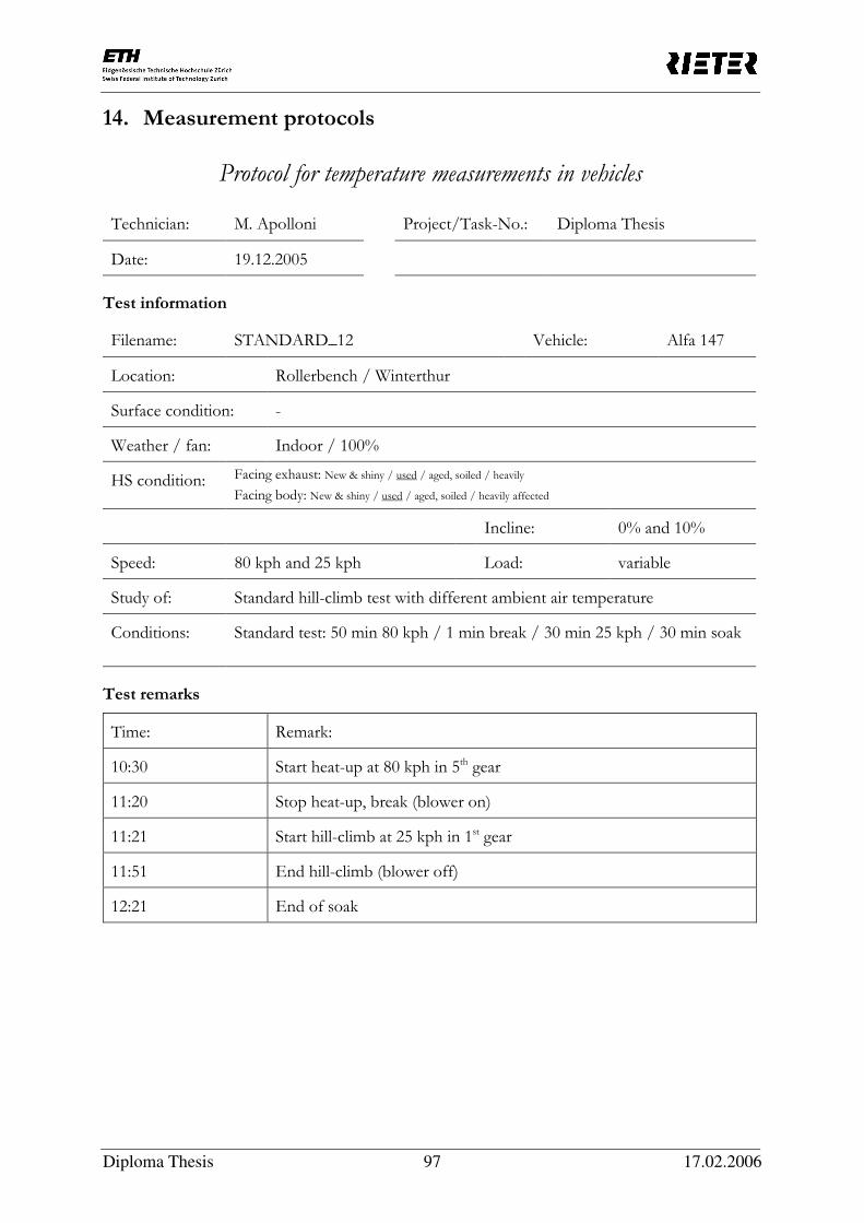
Diploma Thesis 97 17.02.2006
14. Measurement protocols
Protocol for temperature measurements in vehicles
Technician: M. Apolloni Project/Task-No.: Diploma Thesis
Date: 19.12.2005
Test information
Filename: STANDARD_12 Vehicle: Alfa 147
Location: Rollerbench / Winterthur
Surface condition: -
Weather / fan: Indoor / 100%
HS condition: Facing exhaust: New & shiny / used / aged, soiled / heavily
Facing body: New & shiny / used / aged, soiled / heavily affected
Incline: 0% and 10%
Speed: 80 kph and 25 kph Load: variable
Study of: Standard hill-climb test with different ambient air temperature
Conditions: Standard test: 50 min 80 kph / 1 min break / 30 min 25 kph / 30 min soak
Test remarks
Time: Remark:
10:30 Start heat-up at 80 kph in 5th gear
11:20 Stop heat-up, break (blower on)
11:21 Start hill-climb at 25 kph in 1st gear
11:51 End hill-climb (blower off)
12:21 End of soak

Diploma Thesis 98 17.02.2006
Protocol for temperature measurements in vehicles
Technician: M. Apolloni Project/Task-No.: Diploma Thesis
Date: 20.12.2005
Test information
Filename: STANDARD_16 Vehicle: Alfa 147
Location: Rollerbench / Winterthur
Surface condition: -
Weather / fan: Indoor / 100%
HS condition: Facing exhaust: New & shiny / used / aged, soiled / heavily affected
Facing body: New & shiny / used / aged, soiled / heavily affected
Incline: 0% and 10%
Speed: 80 kph and 25 kph Load: variable
Study of: Standard hill-climb test with different ambient air temperature
Conditions: Standard test: 50 min 80 kph / 1 min break / 30 min 25 kph / 30 min soak
Test remarks
Time: Remark:
11:00 Start heat-up at 80 kph in 5th gear
11:50 Stop heat-up, break (blower on)
11:51 Start hill-climb at 25 kph in 1st gear
12:21 End hill-climb (blower off)
12:51 End of soak

Diploma Thesis 99 17.02.2006
Protocol for temperature measurements in vehicles
Technician: M. Apolloni Project/Task-No.: Diploma Thesis
Date: 22.12.2005
Test information
Filename: STANDARD_20 Vehicle: Alfa 147
Location: Rollerbench / Winterthur
Surface condition: -
Weather / fan: Indoor / 100%
HS condition: Facing exhaust: New & shiny / used / aged, soiled / heavily affected
Facing body: New & shiny / used / aged, soiled / heavily affected
Incline: 0% and 10%
Speed: 80 kph and 25 kph Load: variable
Study of: Standard hill-climb test with different ambient air temperature
Conditions: Standard test: 50 min 80 kph / 1 min break / 30 min 25 kph / 30 min soak
Test remarks
Time: Remark:
11:10 Start heat-up at 80 kph in 5th gear
12:00 Stop heat-up, break (blower on)
12:01 Start hill-climb at 25 kph in 1st gear
12:31 End hill-climb (blower off)
13:01 End of soak

Diploma Thesis 100 17.02.2006
Protocol for temperature measurements in vehicles
Technician: M. Apolloni Project/Task-No.: Diploma Thesis
Date: 19.12.2005
Test information
Filename: STANDARD_24 Vehicle: Alfa 147
Location: Rollerbench / Winterthur
Surface condition: -
Weather / fan: Indoor / 100%
HS condition: Facing exhaust: New & shiny / used / aged, soiled / heavily affected
Facing body: New & shiny / used / aged, soiled / heavily affected
Incline: 0% and 10%
Speed: 80 kph and 25 kph Load: variable
Study of: Standard hill-climb test with different ambient air temperature
Conditions: Standard test: 50 min 80 kph / 1 min break / 30 min 25 kph / 30 min soak
Test remarks
Time: Remark:
16:00 Start heat-up at 80 kph in 5th gear
16:50 Stop heat-up, break (blower on)
16:51 Start hill-climb at 25 kph in 1st gear
17:21 End hill-climb (blower off)
17:51 End of soak

Diploma Thesis 101 17.02.2006
Protocol for temperature measurements in vehicles
Technician: M. Apolloni Project/Task-No.: Diploma Thesis
Date: 20.12.2005
Test information
Filename: STANDARD_28 Vehicle: Alfa 147
Location: Rollerbench / Winterthur
Surface condition: -
Weather / fan: Indoor / 100%
HS condition: Facing exhaust: New & shiny / used / aged, soiled / heavily affected
Facing body: New & shiny / used / aged, soiled / heavily affected
Incline: 0% and 10%
Speed: 80 kph and 25 kph Load: variable
Study of: Standard hill-climb test with different ambient air temperature
Conditions: Standard test: 50 min 80 kph / 1 min break / 30 min 25 kph / 30 min soak
Test remarks
Time: Remark:
15:45 Start heat-up at 80 kph in 5th gear
16:35 Stop heat-up, break (blower on)
16:36 Start hill-climb at 25 kph in 1st gear
17:06 End hill-climb (blower off)
17:36 End of soak
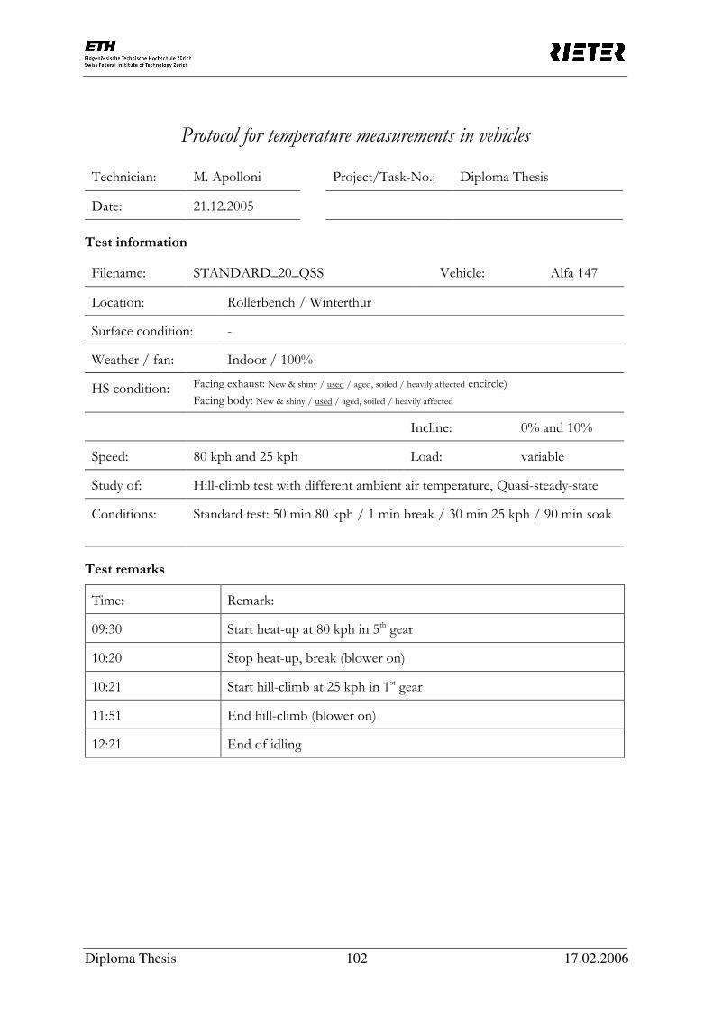
Diploma Thesis 102 17.02.2006
Protocol for temperature measurements in vehicles
Technician: M. Apolloni Project/Task-No.: Diploma Thesis
Date: 21.12.2005
Test information
Filename: STANDARD_20_QSS Vehicle: Alfa 147
Location: Rollerbench / Winterthur
Surface condition: -
Weather / fan: Indoor / 100%
HS condition: Facing exhaust: New & shiny / used / aged, soiled / heavily affected encircle)
Facing body: New & shiny / used / aged, soiled / heavily affected
Incline: 0% and 10%
Speed: 80 kph and 25 kph Load: variable
Study of: Hill-climb test with different ambient air temperature, Quasi-steady-state
Conditions: Standard test: 50 min 80 kph / 1 min break / 30 min 25 kph / 90 min soak
Test remarks
Time: Remark:
09:30 Start heat-up at 80 kph in 5th gear
10:20 Stop heat-up, break (blower on)
10:21 Start hill-climb at 25 kph in 1st gear
11:51 End hill-climb (blower on)
12:21 End of idling

Diploma Thesis 103 17.02.2006
Protocol for temperature measurements in vehicles
Technician: M. Apolloni Project/Task-No.: Diploma Thesis
Date: 21.12.2005
Test information
Filename: MALBUN_20 Vehicle: Alfa 147
Location: Rollerbench / Winterthur
Surface condition: -
Weather / fan: Indoor / 100%
HS condition: Facing exhaust: New & shiny / used / aged, soiled / heavily affected encircle)
Facing body: New & shiny / used / aged, soiled / heavily affected
Incline: 0% and 10%
Speed: 80 kph and 25 kph Load: variable
Study of: Malbun hill-climb test with one ambient air temperature
Conditions: Malbun simulation with three virtual traffic lights
Test remarks
Time: Remark:
15:30 Start heat-up at 80 kph in 5th gear
16:20 Stop heat-up, break (blower on)
16:21 Start Malbun hill-climb at 25 kph in 1st gear
16:30 Break (blower off)
16:31 Continue
16:36 Break (blower off)
16:37 Continue
16:41 Break (blower off)
16:42 Continue
16:50 End Malbun hill-climb (blower off)
17:20 End of soak

Diploma Thesis 104 17.02.2006
15. Measurement positions
MCPS Project Definition
Technician: M. Apolloni Project/Task-No.: Diploma Thesis
Date: 21.12.2005
MCPS no.
Yokogawa type
1: DA 100-1 (30ch) 2: DA 100-2 (60ch) 3: DA 2500 (60 ch) 4: DA 2500 (120 ch)
Yokogawa
channel no.
TC no.
Norm: ANSI
Extension no.
Location
1 3 1 143 V5001 Fan
2 3 2 119 V5002 Exh 2 cat 1 up
3 3 3 78 V5003 Exh 2 cat 1 down
4 3 4 72 V5004 Exh 4
5 3 5 86 V5005 Exh 5
6 3 6 613 V5006 Exh 6 HS
7 3 7 32 V5007 Exh 7
8 3 8 64 V5008 Exh 8
9 3 9 60 V5009 Exh 9 cat 2 (1)
10 3 10 9 V5010 Exh 10 cat 2 (2)
11 3 11 145 V5011 Exh 11 cat 2 (3)
12 3 12 109 V5012 Exh 12
13 3 13 114 V5013 Exh 13
14 3 14 27 V5014 Exh 14
15 3 15 48 V5015 Exh 15
16 3 16 28 V5016 Exh 16
17 3 17 46 V5017 Exh 17 pipe end
18 3 18 140 V5018 Gas 1 after cat 1
19 3 19 141 V5019 Gas 2 before cat 2
20 3 20 142 V5020 Gas 3 after cat 2
21 3 21 116 V5021 Gas 4 pipe end
22 3 22 39 V5022 HS 1a
23 3 23 136 V5023 HS 1b
24 3 24 142 V5024 HS 2a
25 3 25 141 V5025 HS 2b

Diploma Thesis 105 17.02.2006
MCPS
no. Yokogawa
type 1: DA 100-1 (30ch) 2: DA 100-2 (60ch) 3: DA 2500 (60 ch) 4: DA 2500 (120 ch)
Yokogawa
channel no.
TC no.
Norm: ANSI
Extension no.
Location
26 3 26 74 V5026 HS manifold
27 3 27 125 V5027 HS cat 1
28 3 28 65 V5028 Body 1a
29 3 29 49 V5029 Body 1b
30 3 30 47 V5030 Body 2a
31 3 31 67 V5031 Body 2b
32 3 32 115 V5032 Air amb (rearview mirror or blower outlet)
33 3 33 118 V5033 Air exh 2 cat 1
34 3 34 70 V5034 Air exh 6
35 3 35 33 V5035 Air exh 8
36 3 36 66 V5036 Air 9 cat 2 (1)
37 3 37 29 V5037 Air 10 cat 2a (2)
38 3 38 68 V5038 Air 10 cat 2b (2)
39 3 39 146 V5039 Air 11 cat 2 (3)
40 3 40 113 V5040 Air exh 12
41 3 41 139 V5041 Air exh 13a
42 3 42 140 V5042 Air exh 13b
43 3 43 108 V5043 Air HS 1a
44 3 44 8 V5044 Air HS 1b
45 3 45 44 V5045 Air HS 2a
46 3 46 30 V5046 Air HS 2b
47 3 47 127 V5047 Air airfilter
48 3 48 57 V5048 Exh 1 manifold
49 3 49 35 V5049 Body eus 1a
50 3 50 117 V5050 Body eus 1b
51 3 51 73 V5051 Body eus 1c
52 3 52 69 V5052 Body eus 2a
53 3 53 147 V5053 Body eus 2b
54 3 54 149 V5054 Body eus 3a
55 3 55 40 V5055 Body eus 3b
56 3 56 123 V5056 Air eus 1a

Diploma Thesis 106 17.02.2006
MCPS
no. Yokogawa
type 1: DA 100-1 (30ch) 2: DA 100-2 (60ch) 3: DA 2500 (60 ch) 4: DA 2500 (120 ch)
Yokogawa
channel no.
TC no.
Norm: ANSI
Extension no.
Location
57 3 57 75 V5057 Air eus 1b
58 3 58 87 V5058 Air eus 1c
59 3 59 62 V5059 Air eus 2a
60 3 60 88 V5060 Air eus 2b
61 2 101 - V5061 Intercooler out
62 2 102 - V5062 Gas manifold
63 2 103 - V5063 Gas cat 1 in
64 2 104 - V5064 Intercooler in
65 4 105 412 V5065 Exh 8.5
66 4 106 419 V5066 Exh 12.5
67 4 107 414 V5067 Air exh 8.5
68 4 108 424 V5068 Air exh 12.5
69 4 109 438 V5069 HS 0.5b
70 4 110 426 V5070 HS 1.5b
71 4 111 432 V5071 Air HS 0.5b
72 4 112 413 V5072 Air HS 1.5b
73 4 113 431 V5073 Body 0.5b
74 4 114 430 V5074 Body 1.5b
75 4 115 85 V5075 Air hood liner 2b
76 2 116 508 V5076 Front tunnel left
77 2 117 601 V5077 Front tunnel right
78 2 118 606 V5078 Low fan out
79 2 119 500 V5079 Front tunnel middle
80 4 120 107 V5080 Air fan in
81 4 121 79 V5081 Air fan out / Battery
82 4 122 99 V5082 Air wheelarch down L
83 4 123 96 V5083 Air wheelarch up L
84 4 124 103 V5084 Air wheelarch down R
85 4 125 92 V5085 Air wheelarch up R
86 4 126 100 V5086 Engine oil sump
87 4 127 105 V5087 Gearbox oil sump

Diploma Thesis 107 17.02.2006
MCPS
no. Yokogawa
type 1: DA 100-1 (30ch) 2: DA 100-2 (60ch) 3: DA 2500 (60 ch) 4: DA 2500 (120 ch)
Yokogawa
channel no.
TC no.
Norm: ANSI
Extension no.
Location
88 4 128 56 V5088 Battery / Air fan out
89 4 129 128 V5089 Starter
90 4 130 131 V5090 Engine oil
91 4 131 139 V5091 Gearbox oil
92 4 132 129 V5092 Dash a
93 4 133 98 V5093 Dash b
94 4 134 144 V5094 Radiator coolant out
95 4 135 143 V5095 Engine coolant out (bypass)
96 4 136 90 V5096 Air fuse box
97 4 137 0 V5097 V-belt
98 4 138 84 V5098 Cylinder head 1
99 4 139 21 V5099 Cylinder head 2a
100 4 140 31 V5100 Cylinder head 2b
101 4 141 22 V5101 Intake manifold a
102 4 142 26 V5102 Intake manifold b
103 4 143 202 V5103 Engine top cover 1
104 4 144 206 V5104 Engine top cover 2
105 4 145 15 V5105 Engine top cover liner 2
106 4 146 24 V5106 Air engine top cover 1
107 4 147 59 V5107 Air engine top cover 3
108 4 148 55 V5108 Camshaft case
109 4 149 121 V5109 Steering linkage
110 4 150 101 V5110 HS cover 1
111 4 151 155 V5111 Air blower
112 4 152 extern Anemometer speed (behind fan or at blower)
113 4 153 extern Anemometer temperature
114 4 154 extern Vehicle speed
Table G-1: Measurement position for thermal investigation

Diploma Thesis 108 17.02.2006
16. Nomenclature and Abbreviations
Symbol Quantity Unit
a acceleration m/s2
A (cross-section) area m2
cp specific heat at constant pressure J/kgK cv specific heat at constant volume J/kgK cD drag coefficient - cL coefficient for mechanical losses - cR coefficient of rolling resistance - C conductance (per unit rpm) W/K (W/rpmK) d diameter m Dh hydraulic diameter m F force N Fdrag drag resistance N Fgrade grade resistance N Finertia inertia resistance N Froll rolling resistance N g gravity m/s2 h average heat transfer coefficient W/m2K hx local heat transfer coefficient W/m2K h height m i gear ratio - k thermal conductivity W/mK km inertia coefficient - L (characteristic) length m m mass kg mdot mass flow rate kg/s n engine speed rpm pwheel wheel perimeter m P power W P perimeter m p pressure Pa Qdot heat flow rate W q'' heat flux W/m2
r radius m rfuel fuel ratio - raxis axis ratio - rgear gear ratio - R gas constant J/molK s grade % T temperature °C TW coolant water temperature, wall temperature °C Tsat saturation temperature °C ∆T temperature difference °C u, U velocity m/s v vehicle speed m/s v* vehicle speed km/h VH engine swept volume l
w width m Y coolant tube length m

Diploma Thesis 109 17.02.2006
Nu Nusselt number = hL/k (resp. hDh/k) - Pr Prantl number = cpµ/k - Re Reynolds number = UρL/µ (resp. UρDh/ µ) - δ momentum boundary layer thickness m ε view factor - ε heat exchanger effectiveness (definition) - η fin effectiveness - κ thermal diffusivity m2/s µ dynamic viscosity N/m2s ν kinematic viscosity m2/s ν thermostat opening position - ρ density kg/m3
σ standard deviation variable σ Stefan-Boltzmann Konstante W/m2K4 Abbreviation Meaning
EA Evolutionary Algorithm EC Evolutionary Computation amb ambient base baseline CAE Computer Aided Design CFD Computational Fluid Dynamics CoE Center Of Excellence dCi Direct injection diesel ECU Engine Control Unit EGR Exhaust Gas Recirculation eng engine exh exhaust hs heatshield JTD Jet Turbo Diesel MCPS MultiChannel Process System noc number of combinations OEM Original Equipment Manufacturer PLC Programmable Logic Controller qss quasi-steaty-state rad radiator rpm revolutions per minute RSim Rapid target Simulation rtP real-time workshop model parameter structure TC Thermocouple UTM Underhood Thermal Management

Diploma Thesis 110 17.02.2006
17. List of figures and tables
Figure B-1: Transfer function for measurement tests ............................................................. 10
Figure B-2: Profile of hill-climb test from Triesen to Malbun (FL)......................................... 11
Figure B-3: Location of the temperature measurement in the underbody part........................ 12
Figure B-4: On-road test: Exhaust temperatures at position 2 of Skyline................................ 15
Figure B-5: Incline for on-road test drive ............................................................................... 16
Figure B-6: Influence of changing grade and velocity on engine power .................................. 16
Figure C-1: Rollerbench with mounted vehicle....................................................................... 18
Figure C-2: Control room: Ventilation and drive control unit ................................................ 19
Figure C-3: Monitoring of the vehicle temperatures ............................................................... 19
Figure C-4: Long term goal of simulation procedure .............................................................. 20
Figure C-5: Repeatability test for cooling circuit..................................................................... 21
Figure C-6: Repeatability test for underbody region ............................................................... 22
Figure C-7: Difference of ambient air temperatures ............................................................... 23
Figure C-8: Repeatability test for radiator and fan behavior.................................................... 24
Figure C-9: Temperature drift of the ambient air measured at fan air in position.................... 24
Figure C-10: Temperature measurement at fan air in and blower outlet position...................... 25
Figure C-11: Position of controlling thermocouple in the supply air channel ........................... 26
Figure C-12: Underbody sections with tunnel entrance ............................................................ 27
Figure C-13: Air temperatures at the tunnel entrance ............................................................... 28
Figure C-14: Gas manifold temperature for different engine load ............................................ 28
Figure C-15: Gas manifold temperature for different engine speed and load ............................ 29
Figure C-16: Radiator effectiveness during the test cycle .......................................................... 29
Figure C-17: Coolant temperature characteristics ..................................................................... 30
Figure C-18: Body temperatures at different ambient air temperatures for all sections ............. 32
Figure C-19: Body temperature distribution at section 1 corrected by a constant temperature.. 32
Figure D-1: Cooling system of the vehicle .............................................................................. 33
Figure D-2: Oil and coolant circuit of the cooling system ....................................................... 34
Figure D-3: Simulated and measured cooling system temperatures ......................................... 35
Figure D-4: Heat transfer coefficient calculation for underbody boundary layer ..................... 37
Figure D-5: Boundary layer thickness of flat plate................................................................... 37
Figure D-6: Node system of the 1-D model ........................................................................... 39
Figure D-7: Rotational inertia coefficient ................................................................................ 40
Figure D-8: Engine calculation subsystem .............................................................................. 41
Figure D-9: Load calculation subsystem ................................................................................. 41
Figure D-10: Thermostat hysteresis and linear model ............................................................... 42
Figure D-11: Thermostat position subsystem ........................................................................... 43
Figure D-12: Fan state calculation ............................................................................................ 43
Figure D-13: Overview: Fan demand, fan state and thermostat position................................... 44
Figure D-14: Fan demand subsystem........................................................................................ 44
Figure D-15: Radiator airflow subsystem .................................................................................. 44
Figure D-16: Thermodynamic balance of heat dissipation ........................................................ 45
Figure D-17: Limitation of fin effectiveness ............................................................................. 48
Figure D-18: Simulink signal builder......................................................................................... 51
Figure D-19: Result of a manual optimization for cooling circuit temperatures......................... 52
Figure D-20: Problem solution using evolutionary algorithm.................................................... 53
Figure D-21: Structure of a single population evolutionary algorithm ....................................... 53
Figure D-22: Structure of an extended multi-population evolutionary algorithm ...................... 54

Diploma Thesis 111 17.02.2006
Figure D-23: Number of combinations for the Simulink model evaluation............................... 56
Figure D-24: Simplified structure of the calculation process ..................................................... 57
Figure D-25: Calculation of quality criteria for the evolutionary algorithm................................ 58
Figure D-26: New measurement data at 20°C ambient temperature ......................................... 59
Figure D-27: Sensitivity analysis for the 22 guessing parameters ............................................... 60
Figure D-28: Changed simulation model .................................................................................. 62
Figure D-29: New result for changed model............................................................................. 62 Figure D-30: Real ambient air temperature, constant ambient at 19°C, constant ambient at
20°C and constant ambient at 21°C ..................................................................... 63
Figure D-31: Simulation of a constant velocity ......................................................................... 64
Figure D-32: Coolant temperature increase for the hill-climb test............................................. 64
Figure D-33: Fin effectiveness versus radiator effectiveness during simulation ......................... 65
Figure D-34: Temperature pattern of engine coolant and oil .................................................... 67
Figure D-35: Dissipated heat to coolant and exhaust gas .......................................................... 68
Figure D-36: Qualitative plot for convection and boiling regimes............................................. 69
Figure D-37: Boiling temperature in dependency on overpressure and coolant mixing ratio ..... 69 Figure D-38: Comparison of simulation and measurement for different ambient air
temperatures........................................................................................................ 71
Figure G-1: On-road test body temperatures for all sections................................................... 76
Figure G-2: On-road test heatshield temperatures for all sections ........................................... 78
Figure G-3: On-road test exhaust temperatures for all sections............................................... 80
Figure G-4: Overview: Engine and cooling circuit calculation................................................. 91
Figure G-5: Node temperature calculation for the dynamic system ......................................... 96
Table A-1: Data of simulation tools ........................................................................................ 8
Table B-1: Starting and ending temperatures at body position for all sections ....................... 13
Table B-2: Mean standard deviation of the temperature offsets ............................................ 13 Table B-3: Temperature difference between body and heatshield and between heatshield
and exhaust, respectively...................................................................................... 14
Table B-4: Test procedure for the rollerbench measurements ............................................... 17
Table C-1: Temperature differences for repeatability test ...................................................... 22
Table C-2: Fan activity during the standard test .................................................................... 27
Table D-1: Determining the rotational inertia coefficient ...................................................... 40
Table D-2: Changing parameters with their specific ranges and units .................................... 56
Table G-1: Measurement position for thermal investigation ................................................ 107

Diploma Thesis 112 17.02.2006
H. References
Books:
[1] John H. Lienhard IV and John H. Lienhard V, A Heat Transfer Handbook, 3rd edition, Phlogiston Press, 2002
[2] Vennard J. K. and Street R. L., Elementary Fluid Mechanics, 6th Edition, John Wiley &
Sons, New York, 1982 [3] H. Schlichting and K. Gersten, Boundary Layer Theory, 8th Revised and Enlarged Edition,
Springer, 2003 [4] VDI-Wärmeatlas, Berechnungsblätter für den Wärmeübergang, Verein Deutscher
Ingenieure, VDI-Gesellschaft Verfahrenstechnik und Chemieingenieurwesen (GVC), 8. Auflage, Springer, 1997
[5] Bosch, Automotive Handbook, 6th Edition, Robert Bosch GmbH, 2004
Scripts:
[6] Prof. D. Poulikakos, Thermodynamik I&II, Department of Mechanical Engineering, SS2002
[7] Prof. K. Boulouchos, Arbeitsprozesse instationärer Verbrennungskraftmaschinen, SS2004
Technical papers:
[I] Hermann de Ciutiis, Effect of an Optimized Heatshield Design and an Aerodynamic Exhaust Tunnel Cover on Convective Heating of the Floor Pan, Rieter Automotive Management AG, Switzerland, Vehicle Thermal Management System 7 Conference: 2005-01-2016, 2005
[II] Ed Bendell, Investigation of a Coupled CFD and Thermal Modeling Methodology for Prediction of
Vehicle Underbody Temperatures, Rieter Automotive Management AG, Switzerland, Vehicle Thermal Management System 7 Conference: 2005-01-2044, 2005
[III] Ernst Peter Weidmann, Jochen Wiedemann, Thomas Binner, and Heinrich Reister,
Underhood Temperature Analysis in Case of Natural Convection, Research Institute of Automotive Engineering and Vehicle Engines, Stuttgart (FKFS), DaimlerChrysler AG, Vehicle Thermal Management System 7 Conference: 2005-01-2045, 2005
[IV] Francesco Fortunato, Fluvio Damiano, Luigi Di Matteo and Paolo Oliva, Underhood
Cooling Simulation for Development of New Vehicles, Elasis S.C.p.A., PWT, Engine Systems, Vehicle Thermal Management System 7 Conference: 2005-01-2046, 2005
[V] Anders Jönson, Balancing Thermodynamic and Aerodynamic Attributes Through the Use of a
Common CFD Model, Volvo Car Corporation, Vehicle Thermal Management System 7 Conference: 2005-01-2052, 2005

Diploma Thesis 113 17.02.2006
[VI] H. Reister and M. Maihöfer, Underhood component temperature analysis for passenger cars, DaimlerChrysler, Sindelfingen, Germany, Vehicle Thermal Management System 6 Conference: C599/028/2003, 2003
[VII] M. Schuster, Application of CFD as an efficient analysis tool supporting the experimental
investigation of underhood and underbody vehicle flows, AUDI AG, Ingolstadt, Germany, Vehicle Thermal Management System 6 Conference: C599/056/2003, 2003
[VIII] A. Skea, A. Jolliffe, R. Harrison, M.R. Jones, P. Cardani, and L. Smith, Integrated
underbonnet thermal management simulation, MIRA Limited, Nuneaton, UK, Vehicle Thermal Management System 6 Conference: C599/074/2003, 2003
[IX] K. Srinivasan, Z. J. Wang, W. Yuan and R. Sun, Vehicle Thermal Management Simulation
Using a Rapid Omni-tree Based Adaptive Cartesian Mesh Generation Methodology, DaimlerChrysler Corporation, Michigan, USA, ASME Heat Transfer/Fluids Engineering Conference: HT-FED2004-56748, 2004
[X] G.P. Hammond, Turbulent Prandtl Number Within a Near-Wall Flow, Crunfield Institute
of Technology, Bedford, England, AIAA Journal: 0001-1452 vol. 23 no. 11 (1668-1669), 1985
[XI] T. Mark, David Knott and J. Walter, Transitioning Automotive Testing from the Road to the
Lab, Ford Motor Company, SAE World Congress: 2004-01-1770, 2004 [XII] Hartmut Pohlheim, GEATbx Introduction, Evolutionary Algorithms: Overview, Methods and
Operators, http://www.geatbx.com, 2005 [XIII] Christopher Depcik and Dennis Assanis, A Universal Heat Transfer Correlation for
Intake/Exhaust Flow in a Spark Ignition Internal Combustion Engine, University of Michigan, SAE: 2002-01-0372, 2002
[XIV] V. C. Aute, D. Richardson, R. Radermacher and J. Hager, Vehicle thermal systems
optimization using genetic optimization algorithms, University of Maryland College Park, USA, Vehicle Thermal Management System 6 Conference: C599/076/2003, 2003
[XV] A. Piccolo, L. Ippolito, V. zo Galdi and A. Vaccaro, Optimization of energy flow management
in hybrid electric vehicles via genetic algorithms, IEEE/ASME International Conference on Advanced Intelligent Mechatronics, New Jersey, USA, p. 434-9, 2001
[XVI] Chen Bi-feng, Lu Hao-juan and Huang Zhang-can, A model and its algorithm to search the
best route in a vehicle navigation system, Wuhan University of Technology, vol. 24, no. 3, p. 46-8, 2002
[XVII] J. R. Hull, Efficient Cooling in Engines with Nucleate Boiling, Argonne National Laboratory,
Ilinois, USA, U.S. Department of Energy, annual report, 2003 [XVIII] Changhua Lin, Jeffrey Saunders and Simon Watkins, The Effect of Changes in Ambient and
Coolant Radiator Inlet Temperatures and Coolant Flowrate on Specific Dissipation, SAE World Congress: 2000-01-0579, Detroit, Michigan, 2000

Diploma Thesis 114 17.02.2006
I. Acknowledgements
At the end of my Diploma Thesis, I would like to express my thanks to several people who were involved in this project:
First, I want to thank my tutor Mr. Hermann de Ciutiis, Head of Thermal Management at Rieter Automotive, who gave me the possibility to work out an actual problem of their group.
Special thanks go to the group of Thermal Management, namely Mr. Ed Bendell, Mr. Michael Hauenstein, Mr. Luka Gorlato and Mr. Thomas Bürgin. Mr. Bendell supported me highly in this project and I want to thank him for all the interesting discussions and inputs. Thanks go to Mr. Hauenstein who helped me out with problems concerning Matlab/Simulink and Linux operating system. Mr. Gorlato and Mr. Bürgin supported me in any problem concerning the experimental part of the project.
Furthermore, I want to thank Mr. Paolo Bertolo and Mr. Davide Caprioli from the acoustic group for all their work concerning the evolutionary algorithm.
Finally, I want to thank Prof. Dr. Aldo Steinfeld for his acceptance for elaborating my Diploma Thesis in the industry.