research in nonlinear flight control for … research in nonlinear flight control for tiltrotor...
TRANSCRIPT
NASA-CR-203112
RESEARCH IN NONLINEAR FLIGHT CONTROLFOR TILTROTOR AIRCRAFF
OPERATING IN THE TERMINAL AREA.
Progress Report #1November 1996
1 September 1995 - 31 August 1996
/ J ,
3 S.2_0
Research supported by the NASA Ames Research CenterNASA Cooperative Agreement No. NCC 2-922
Principal Investigator:Research Assistant:NASA Grant Monitor:
Dr. A. J. Calise
R. RysdykDr. R. Chen
School of Aerospace EngineeringGeorgia Institute of TechnologyAtlanta, Georgia 30332
https://ntrs.nasa.gov/search.jsp?R=19970007336 2018-06-28T07:52:32+00:00Z

Contents
1 Background 5
2 Flight Control Augmentation 62.1 Rate Command and Attitude Command ........................ 7
2.2 Attitude Hold ....................................... 7
2.3 Augmentation for an Instrument Approach ...................... 7
3 Low Order Pilot Models for Longitudinal Operation of a Tiltrotor Aircraft 8
3.1 Tiltrotor Aircraft Low Order Response Approximations ............... 9
3.2 Pilot Model Design .................................... 13
3.3 Pilot Performance in Different Phases of Flight .................... 273.4 Conclusion ........................................ 30
Implementation of Neural Net Work Augmented Model Inversion 32
4.1 Neural Network Augmented Model Inversion ..................... 324.2 Numerical Results .................................... 35
5 Further Development 41

List of Tables
Combinations of control augmentation response types ................. 6V-22 tilt rotor control augmentation response types .................. 6
Vertical rate response model parameter values at 30 Kts ................ 10
List of Figures
1 Control with attitude hold augmentation ........................ 7
2 Powercurve for different configurations ......................... 9
3 Udot/dxln step response at 30 Kts ............................ 104 Hdot/dxcol step response at 30Kts ............................ 11
5 Hdot/dxln step response at 180 Kts ........................... 12
6 E/dxcol step response at 180 Kts ............................ 12
7 Closed loop of pilot model with aircraft ......................... 13
8 Implementation of pilot models .............................. 149 Blending of pilot models ................................. 14
10 Pilot model for speed in helicopter configuration .................... 15
11 Root locus for helicopter speed control ......................... 1512 Pilot performance for 10 Kts step in Udes in helicopter configuration ........ 16
13 Pilot control activity for a l0 Kts step in Udes in helicopter configuration ...... 16
14 Pilot model for altitude in helicopter configuration ................... 18
15 Altitude loop root locus, mild (T,,tl = lOsec) pole locations .............. 18
16 Altitude loop root locus, aggressive (T,,a = 3sec) pole locations ........... 19
17 Pilot performance for 25 ft step in Hdes in helicopter configuration with mild and
aggressive pilot model design ............................... 1918 Collective control activity for 25 ft step in Hdes in helicopter configuration with
mild and aggressive pilot model design ......................... 20
19 Vertical rate in helicopter configuration ......................... 2020 Pilot performance for 16.7 ft/s step in R.O.C. in helicopter configuration ...... 2021 Vertical rate to altitude control transition ........................ 21
22 Pilot performance -200 ft step in altitude in helicopter configuration ......... 2123 Pilot control activity for -200 ft step in altitude in helicopter configuration ..... 21
24 Pilot model for vertical rate in airplane configuration ................. 23
25 Hd/Hddes in response to 1000fpm step ......................... 2326 Altitude profile in response to Hdes +1000 ft at 180 Kts ................ 23
27 Rate of climb in response to Hdes +1000ft at 180 Kts ................. 24
28 Pilot control activity in response to Hdes +1000ft at 180 Kts ............. 2429 Pilot model for control of energy in airplane configuration ............... 25
30 Pilot performance for step in Udes in airplane configuration .............. 26
31 Pilot control activity for step in Udes in airplane configuration ............ 26
32 Conversion from forward flight into transition with a -.1G force deceleration. Mast
angle, velocity and altitude profiles ........................... 27

33 Conversionfromforwardflightintotransitionwitha-.1G force deceleration. Mast
angle, and pilot activity .................................. 28
3'1 Conversion from transition flight into helicopter configuration. Mast angle, velocityand altitude profiles .................................... 28
35 Conversion from transition flight into helicopter configuration. Mast angle, and pilotactivity ........................................... 29
36 Simulated final approach descent at 30 Kts in helicopter configuration ........ 29
37 Velocity error and control activity during a final approach descent at 30 Kts in
helicopter configuration .................................. 30
38 Neural network augmented model inversion architecture for the implementation oflongitudinal ACAH control ................................ 32
39 Pitch angle response at 30 Kts ............................. 37
40 Actuator activity at 30 Kts ............................... 37
41 Pitch augmentation error at 30 Kts ........................... 37
42 NNW weight adaptation time histories ......................... 3743 Pitch angle response at 30 Kts with errors in inversion model ............ 38
44 Actuator activity at 30 Kts with errors in inversion model .............. 38
45 Pitch augmentation error at 30 Kts with errors in inversion model ......... 38
46 NNW weight adaptation time histories ......................... 3847 Pitch angle response at hover with model inversion based on 30 Kts ........ 39
48 Actuator activity at hover with model inversion based on 30 Kts .......... 39
49 Pitch augmentation error at hover using model inversion based on 30 Kts ..... 39
50 NNW weight adaptation time histories ......................... 3951 Pitch angle response at 100 Kts with model inversion based on 30 Kts ....... 40
52 Actuator activity at 100 Kts with model inversion based on 30 Kts ......... 40
53 Pitch compensation error at 100 Kts with model inversion based on 30 Kts .... 40
54 NNW weight adaptation time histories ......................... 40

Summary
The research during the first year of the effort focused on the implementation of the recently
developed combination of neural net work adaptive control and feedback linearization. At the
core of this research is the comprehensive simulation code Generic Tiltrotor Simulator (GTRS)
of the XV-15 tiltrotor aircraft. For this research the GTRS code has been ported to a Fortranenvironment for use on PC.
The emphasis of the research is on terminal area approach procedures, including conversion
from aircraft to helicopter configuration. This report focuses on the longitudinal control which is
the more challenging case for augmentation. Therefore, an attitude command attitude hold (ACAH)control augmentation is considered which is typically used for the pitch channel during approach
procedures.
To evaluate the performance of the neural network adaptive control architecture it was necessaryto develop a set of low order pilot models capable of performing such tasks as,
• follow desired altitude profiles,
• follow desired speed profiles,
• operate on both sides of powercurve,
• convert, including flaps as well as mastangle changes,
• operate with different stability and control augmentation system (SCAS) modes.
The pilot models are divided in two sets, one for the backside of the powercurve and one for the
frontside. These two sets are linearly blended with speed. The mastangle is also scheduled with
speed.
Different aspects of the proposed architecture for the neural network (NNW) augmented model
inversion were also demonstrated. The demonstration involved implementation of a NNW ar-chitecture using linearized models from GTRS, including rotor states, to represent the XV-15 at
various operating points. The dynamics used for the model inversion were based on the XV-15
operating at 30 Kts, with residualized rotor dynamics, and not including cross coupling betweentranslational and rotational states. The neural network demonstrated ACAH control under various
circumstances.
Future efforts will include the implementation into the Fortran environment of GTRS, includ-
ing pilotmodeling and NNW augmentation for the lateral channels. These efforts should lead to
the development of architectures that will provide for fully automated approach, using similar
strategies.

1 Background
The objective of the current research effort is to develop nonlinear flight control algorithmes for
tiltrotor aircraft operating in the airport terminal area. Like no other aircraft, the tiltrotor displays
varying stability and control characteristics. Most conventional flight control architectures provide
for mission specific augmentation but are not flexible enough to ensure significant improvementsover the entire range of operating circumstances. In the case of tiltrotor aircraft, examples include
the transition from fixed wing to rotary wing flight, mixing of controls, and the possible failure ofactuators and its consequences. In the course of this research several levels of the flight control
will be investigated. These include inner loop SCAS at the lowest level, automated degrees of
freedom at the medium level, and at the highest level fully automated trajectory following control
in the airport terminal area. The study encompasses all flight modes including helicopter mode,transition and airplane mode. A key aspect of this study is the accomodation of modeling error
and failure modes. Therefore, recent developments in combining NNWs and feedback linearization
will be exploited. The research builds upon the NNW flight control studies that have been done
at Georgia Tech to date. These studies addressed;
• Full envelope flight control design without the need for gain scheduling,
• real time adaption to uncertain nonlinear effects, and
• the ability to adapt to partial failures in actuators.
The use of adaptive NNWs in these studies represent a unique application in the aerospace fieldin the sense that they are online, adapting while controlling, with guaranteed stability properties.
The stability properties derive from Lyapunov theory used in the design of the learning rules for
the adaptation of the NNW. Similar control strategies where successfully applied to comprehensive
simulations of an F/A-18 airplane [1] and an AH-64 helicopter [2]. A SCAS system for a tiltrotor
aircraft with its ability to convert from airplane to helicopter configuration, is the ideal candidateto benefit from a control architecture as presented in the current research effort.

2 Flight Control Augmentation
In this report two types of control augmentation are mentioned, Rate Command Attitude Holdand Attitude Command Attitude Hold. These specifications each cover two aspects of the response
to a particular input, the Command and the Hold or Stabilization part. Table 1 shows various
types of augmentation for different channels, ordered from least to most stabilization. Reference
[3] gives the full time automatic flight control system features for the V-22 tiltrotor aircraft. Thisis summarized in table 2.
Table 1: Combinations of control augmentation response types,
from least to most stabilization, from [4].
Response Type: Used for:
1 Rate
2 ACAH+RCHH3 ACAH+RCHH+RCAItH
4 Rate+ RCH H+RCAItH+PosH
5 ACAH+RCHH+RCAItH+PosH
6 TRC+RCHH+RCAItH+PosH
where,Rate
TC
ACAH
RCAItH
HH
RCHH
PosH
TRC
Vertical T/O and transition clear of earth
Slope Landing, precision vertical landing
Precision hover and vertical T/O and transitionTasks involving 'divided attention'
Rapid hovering turn
Hover and taxi, vertical T/O and transition
= Rate or Rate Command Attitude Hold (RCAH)= ]'urn Coordination
= Attitude Command Attitude Hold
= Rate Command Altitude Hold
= Heading Hold
= Rate Command Heading Hold
= Position Hold response type= Translational Rate Command
Table 2:V-22 tilt rotor control augmentation response types.
Hover Fwd FlightAxis Command Hold Command Hold
Pitch
Roll
Wing LvlrYaw
HH Off
Thrust/Pwr
Att Att
Rate AttAtt Att
Rate HH
Rate RateThrust Vert. Rate
'Att' Att
Rate AttAtt Att
Lat Acc HH/TCLat Acc TCThrust

2.1 Rate Command and Attitude Command
Reference[4]definestheCommand part of the augmentation by considering a control stepinput. A control system with a SCAS setting referred to as Altitude-Command implies that the
aircraft responds with a proportional attitude given a step control input. Similarly, a control
system with a SCAS setting referred to as Rate-Command implies that the aircraft responds with
a proportional attitude rate of change given a step control input.
2.2 Attitude Hold
Altitude Hold, also referred to as Attitude Stabilization, is defined using a pulse input into the
primary control, see figure 1. It implies that the aircraft attitude will be returned to its original
value, given no other inputs.
1.8
+t0,8
i i i_ 1'0
1.5
:!f+i0 _ _ _ _ _ _ -' _ ,o
T_m@
Figure 1: Control with attitude hold augmentation.
2.3 Augmentation for an Instrument Approach
Reference [5] describes two experiments with a 40,000 lbf civil tiltrotor piloted simulation
on _steep instrument approaches. The control system is indicated as an ACAH for pitch and
roll, and the yaw axis augmentation included Heading Hold at speeds smaller than 40 Kts and
Turn Coordinalion at speeds bigger than 80 Kts with linear blending between them. This articlerepresents an example for typical approach procedures that a pilot might follow in performing
terminal area operations with a civilian tiltrotor aircraft. The considerations involved in such a
procedure include;
• a schedule for conversion of mast angle with speed, from airplane to helicopter in the
regular approach and vice versa for a missed approach procedure,

• deployment or retraction of flaps depending on mastangle, speed, and glide slope,
• switching from RCAH to ACAH augmentation mode,
• desired altitude and speed trajectories.
Reference [5] and the considerations listed here were used to develop the set of pilot models de-scribed in section 3.
3 Low Order Pilot Models for Longitudinal Operation ofa Tiltrotor Aircraft
To evaluate the performance of a neural network adaptive control architecture it will be neces-
sary to provide for a pilot model. This pilot model should be able to operate the tiltrotor smoothly
in various parts of the operating envelope. Therefore, the objective is to create such a model that
can be tailored to specific tasks, and configured to respond slow enough to maintain a distinctionbetween inner loop network adaptive control and pilot, activity. The model is to perform such tasks
as,
• follow desired altitude profiles,
• follow desired speed profiles,
• operate on both sides of powercurve,
• convert, including flaps as well as mastangle changes,
• operate with different SCAS modes.
This section describes a combination of low order pilot models for the longitudinal channels only.
The pilot model consists of two parts, one backside pilot (BSP) and one frontside pilot (FSP).These two parts are linearly blended with speed. The results using this pilot show:
• Conversion both ways can be achieved with reasonable tracking.
• Fairly aggressive accelerations and climb rates can be achieved.
• The pilot model can be adjusted for different operating circumstances.
• The pilot model can be modified to reflect more accurately the physiological and psy-chological behaviour of a human being. However, the emphasis in this work is on
operation of the vehicle.
The airplane considered will be operated with stabilizing SCAS systems. Furthermore, the ma-
neuvers considered here are not aggressive and do not need modeling of the fast characteristics
of neurological and muscular time constants. The longitudinal pilot models were adjusted for op-
eration under an ACAH SCAS, described in section 2. This mode does not work well at higherspeeds when trying to maintain a desired altitude and speed. A setup that allows for switching

betweenmodesat certainoperatingpointsneedstobeadded.A similarlateralpilotalsoneedstobecreated.However,the longitudinalmodelingproblemisfar morechallengingthanthelateralproblem.
3.1 Tiltrotor Aircraft Low Order Response Approximations
The true aircraft is represented by the Generic Tiltrotor Simulation program that was jointlydeveloped by NASA and Boeing. The model represents the XV15 tiltrotor aircraft. This aircraft
can operate both as a conventional helicopter, and as a regular airplane for the higher speeds. In
this modeling work the pure helicopter mode is used under 60 Kts and the pure airplane mode isused above 120 Kts. The possibility to convert between the two modes requires operation on both
sides of the powercurve. From a modelling perspective that means a total change in the function
of the controls and the associated responses of the aircraft. This section describes the aircraft
responses to inputs in the longitudinal control channels in the two different configurations.
Powercurve
The powercurve refers to the graph of power required versus flight speed. The typical curve
for a helicopter shows a need for high power at hover, due to the powered lift condition. Asshown in figure 2, the need for power decreases as the speed increases. This trend continues
until the aerodynamic drag becomes the dominant factor at higher speeds. The lowest point
of the powercurve for a tiltrotor occurs between the helicopter and airplane configuration. The
significance of the powercurve is in the fact that it demands a different control strategy at thedifferent operating points along the curve. The change in control strategy is centered around the
lowest point of the powercurve. For the conversion schedule used in this work this point occursbetween 70 and 100K/s. Not all the subtleties associated with the powercurve are considered here.
However, it did lead to the idea of the pilot blending. The blending architecture is described insection 3.2.
t_Sdeg
J eOd_g
100vIimi¢ ¢ [K_]I Y,O 200
Figure 2: Powercurve for different configurations.

Longitudinal Stick Command Response, Helicopter Configuration
In helicopter configuration the speed is controlled by a deflection of the longitudinal stick. A
positive deflection is forward, which results in a positive acceleration of the helicopter. As the
speeds increases, so does the aerodynamic drag, therefore a step response in the longitudinal stick
results in the acceleration profile illustrated in figure 3. A low order model of this behaviour is
given by,0 IQ_s
_zln -- S2 d" al s + ao (1)
or equivalently,
with parameters,
U ]x'aem
6zzn s2 + als + ao(2)
h'_c = 3.0
al = 1.02ao = .06
2
t
I • ,*
Figure 3: Udot/dxln step response at. 30 Kts.
Power Lever Command Response, Helicopter Configuration
The response to a step input to the collective lever is illustrated in figure 4. This suggests that
the response is first order, and can be accurately modeled using,
h Iiae- (3)
_=eot s "t- c
Some relevant parameter values at different airspeeds are given in the table 3. The pilot model
development in the next section was based on the values at 30 Kts.
10

7
4
a i iol I12 141 161 181 2o
Timo [ooc]
Figure 4: Hdot/dxcol step response at 30Kts.
Table 3: Vertical rate response model parameter values at 30 Kts.
v [Kts] K [(/t/s)/i./8] c [8-1]0 2.26 .19
30 4.25 .5070 4.75 .625
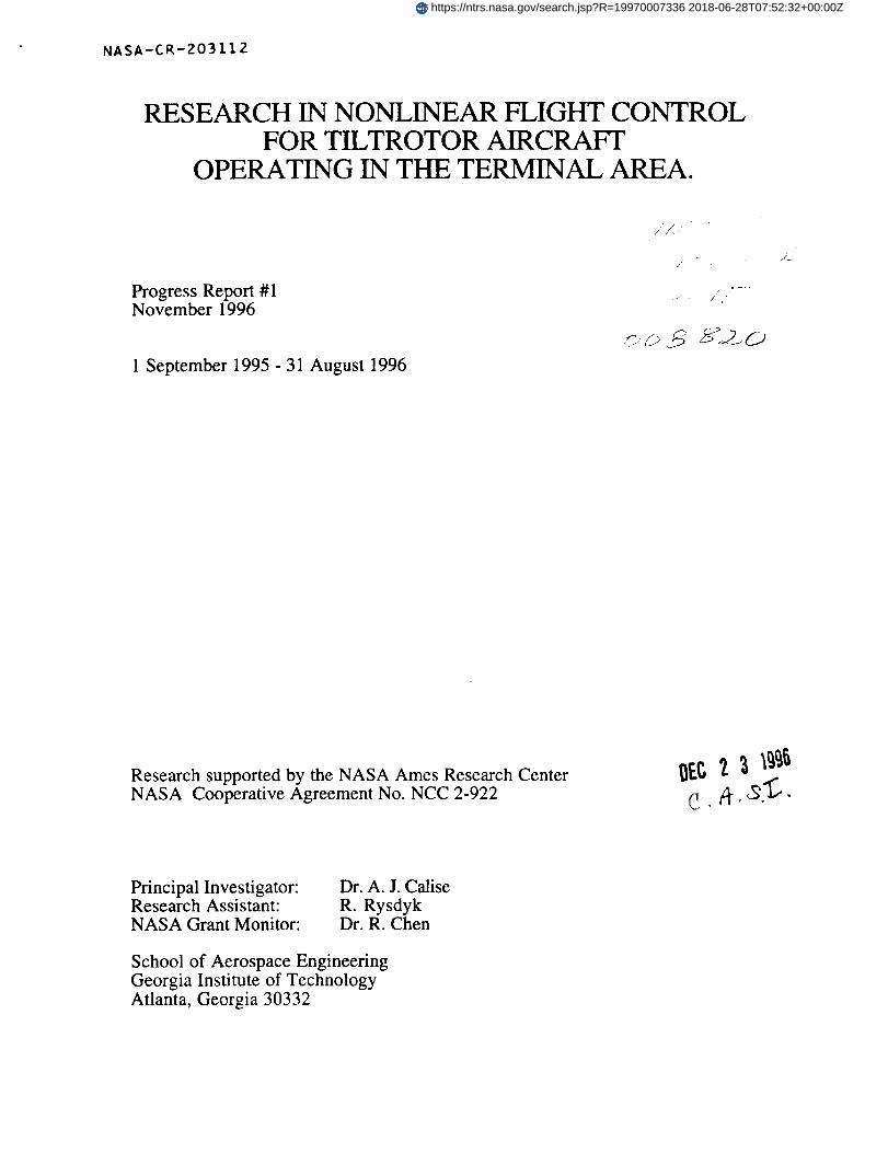
Longitudinal Stick Command Response in Airplane Configuration
In airplane configuration the longitudinal stick is used for altitude control. The primary effect
of a longitudinal input is a pitch change. Thus the pilot is controlling altitude as a secondary
effect. Another secondary effect due to longitudinal stick input is a change in velocity. The stepresponse to longitudinal stick input in forward flight is illustrated in figure 5. The second order
model is given by,/:/ -li,c • s
_z,, -- s_ + als + ao (4)
In terms of altitude control this is equivalent to,
H -Kac
6,_,, - 82 + als + ao (5)
The parameters were found to be,al = .54
a0 = .0329K_¢ = -15.28
ll
t
Figure 5: Hdot/dxln step response at 180 Kts.
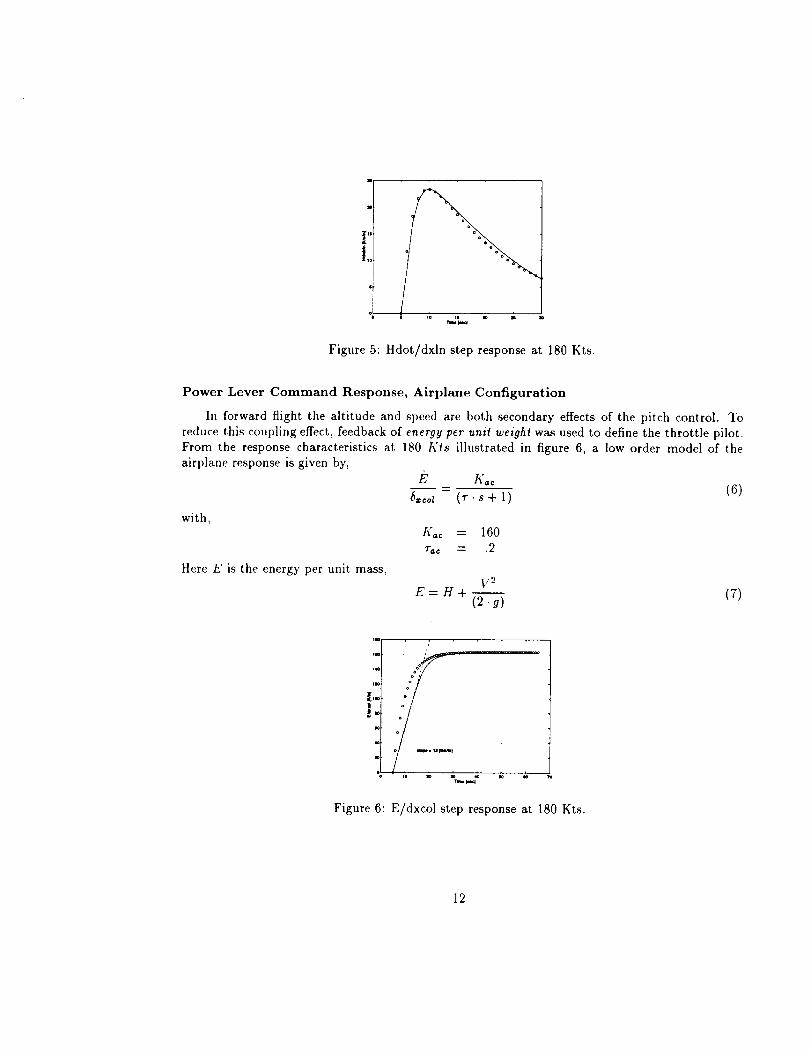
Power Lever Command Response, Airplane Configuration
In forward flight the altitude and speed are both secondary effects of the pitch control. To
reduce this coupling effect, feedback of energy per unit weigM was used to define the throttle pilot.From the response characteristics at 180 Kts illustrated in figure 6, a low order model of the
airplane response is given by,
- (6)_,:oz (r. s + l)
with,
Here E is the energy per unit mass,y 2
I
E=H+ (2.g) (7)
Iw
j:Io
1o
Figure 6: E/dxeol step response at 180 Kts.
12

3.2 Pilot Model Design
The pilot model was developed on the basis of the following form for the pilot transfer function
O_. = z<p.(_+ #)(_ + o,) (8)
This form permits the pilot to be represented as either a lead compensator, a lag compensator,or a P+I controller. As illustrated in figures 7 and 8, the pilot models will be implemented in a
closed loop with the aircraft. The same transfer function form is used to model pilot response to
airplane response in the form of the stick and power lever input.
The pilot models for the helicopter configuration are combined with those for the airplane
configuration through convex blending. The convex blending is linear, as indicated in figure 9, andimplemented as follows
6, = (1 - o0 . 6n,_i + _ • 6Ai,pZ,_ (9)
where,c_ = 1 if V > VII
v-vz if V1 < V < VIIOt -- VII-VI -- --
= 0 if V < VI
with V representing the aircraft speed, and the authority for the helicopter and airplane pilots
represented respectively by the weights, (1 - o_) and _. The low speed pilot models have full
authority at 30 Kts and below. The the high speed models have full authority at 140 Kts andabove. This choice of VI and Vll reflects the fact that the lowest point in the powercurve occurs
between 70 and 100 Kts, depending on the conversion schedule, and flight configuration.
Root locus methods were used to select desirable closed loop characteristics. The pilot modelsare represented here in continuous time. The actual implementation in the Generic Tiltrotor
Simulation is a .Olsec zero order hold discrete time representation.
Gplt
Figure 7: Closed loop of pilot model with aircraft.
13

"Pilot".. .......................... ,
.do_,_iII ! +,..°,orAi._._,l_-
Figure 8: Implementation of pilot models.
100 %
tAuthority
0%
Gplt2 & 4, Heli.
Gpltl & 3, Airpln.
VISpeed------_
VII
Figure 9: Blending of pilot models.
14

Pilot for Speed Control in Helicopter Configuration
The speed at hover is controlled by the longitudinal stick input. The tiltrotor in helicopter
configuration at 30 Kts was found to behave as follows,
U KacB
6¢b, s2 + als + ao(10)
where,l(_c = 3.0
al = 1.02
a0 = .06
The design of the pilot is based on the pilot acting as a P+I controller. A blockdiagram representing
the closed loop is shown in figure 10. Figure 11 shows root loci plots for two values of/L Selecting( = .9 and wn = .33 for the dominant closed loop poles results in
and,.1. (s + .15)
Gplt --$
The performance is shown as a response to a step in Udes in figures 12 and 13.
Vdesdxln
K ac
s2+ a ts + ao
Figure 10: Pilot model for speed in helicopter configuration.
!
Figure 11: Root locus for helicopter speed control.
15

_0 m b_l_ *a In m• J
Figure 12: Pilot performance for 10 Kts step in Udes in helicopter configuration.
-I
-a
-4
i
Figure 13: Pilot control activity for a 10 Kts step in Udes in helicopter configuration.
16

Pilot for Altitude Control in Helicopter Configuration
The pilot model for the collective control was optimized for operation point at 30 Kts, at
13,000 lbf and a flap/flaperon setting of 40o/25 °. Test inputs into the collective lever of the
aircraft showed its vertical rate response to be,
4.256ffic0_ s + .5
The blockdiagram of the altitude pilot is shown in figure 14. This is a type 1 system. The closedloop transfer function is given by
H +/3)Hal,, -- sa + s2(a + c) + s(a .c + k) + _'/3 (11)
where /_" = l_'_c . l(pu = 4.25 • Kplt, and c = .5. The steady state error is zero if the first order
model for the vertical rate is a reasonable representation. The design for this model resulted in
K_u = .75a = 2.9
/3 -- .8
Once a selection of a and/3 is made, the gain can be adjusted for mild or more aggressive pilotbehaviour. From a root locus analysis of GpuG,_ it is possible to select, for example, a Toe_l
lOsec, _ = 1 or a T°,tl ,_ 3see, _ = .7. The root locus of G_aG_c for these examples is given infigures 15 and 16. A milder setting for the model is then,
li'pu = .075= 2.9
¢_ -- .8
with a _ = 1 and wn = .3. The pilot performance is displayed in figures 17 and 18.
In a large altitude or flight level change, a human pilot will use the vertical speed indicator to
monitor the rate of descend. The closed loop transfer function of the vertical rate control loop athover, from figure 19, is
/_ K(s +/3)
/_d,0 - s+ (_ +c+/;:)s +(_.c+/3_') (12)
Here the desired response can be determined by selecting,
(c, + c+ l;=Kp) =2-e + KooKp/3) =
Selecting a = 0 to obtain zero steady state error, with c = .5 and K_ = 4.25 the current design
is based on ( = .9 and w,_ = 1.5, thus giving lipu = .35, and/3 = .8. The resulting performance
to a lO00fprn step in R.O.C. is shown in figure 20. The response to a requested change in flightlevel would require the pilot to initially establish a desired vertical rate, then once the desired new
17

altitudeisalmostestablishedthepilot will concentrateon thealtimeteragain.Thisstrategyisreflectedin a convexblendingof thealtitudeandratemodelsdescribedabove,asindicatedinfigure21.Theconvexblendingis linearandimplementedasfollows,
6.,oZ = (1 - 71) • 6=corn + r/. 6=col_ (13)
where,o = 1 ff R > 50
x-_s if 25 < /_ < 50r] -- 50-_5 - -= 0 if f-1 < 25
with /_ = Hd. - H the altitude error signal. A combination of this rate and altitude response is
shown in figures 22 and 23.
Hdes (s+13)Kph (S+_)
dxcol K ac
(S + C)
Figure 14: Pilot model for altitude in helicopter configuration.
!l
-0
i i-1-S3 -25 -2 -15
Reel Juol-1 -05
Figure 15: Altitude loop root locus, mild (T,,u = lOsec) pole locations.
18

!
-O 1
a:o
Figure 16: Altitude loop root locus, aggressive (T, etz = 3sec) pole locations.
104_
1035
1030
1025
1015
10(16
i i L n J6 10 IS 20 2S
Tt_[_el
Figure 17: Pilot performance for 25 ft step in Hdes in helicopter configuration with mild and
aggressive pilot model design.
19

J
s lo is 20 2s 3oTn I_1
Figure 18: Collective control activity for 25 ft step in Hdes in helicopter configuration with mild
and aggressive pilot model design.
Hales (s+p)Kplt (s +a)
dxcol K ac
(s ÷ c)
Figure 19: Vertical rate in helicopter configuration.
io._
S tO 15 20 _5 30Tw, o l_,:l
Figure 20: Pilot performance for 16.7 ft/s step in R.O.C. in helicopter configuration.
2O

A r_ _m_
r_ hksld _u_dc
Figure 21: Vertical rate to altitude control transition.
360
3OO
2SO
z
1SO
loo
SO
0
T_=_ 4O SO 6O10 2O =e¢]
Figure 22: Pilot performance -200 ft step in altitude in helicopter configuration.
T,v*{_l
Figure 23: Pilot control activity for -200 ft step in altitude in helicopter configuration.
21

Pilot for Altitude Control in Airplane Configuration
The longitudinal channel at forward flight showed a second order response as follows,
The parameters were found to be,
_ _ (14)Gae 6=in s2 -{-al s + ao
al = .54
a0 = .0329
K_c = -15.28
Selecting T,,a = 6 sec, and ( = .707 as desirable for the dominate closed loop poles results in
I(pu = -.003a = .63
/3 = .46
With this selection the steady state error for a step input is 36%. However, since the altitude pilot
model is blended with a vertical rate pilot model, the altitude steps are limited to 50 ft or less
(see below), which will result in an 18ft deviation. A zero steady state error can be achieved by
setting o = O. A T, etl _ 12sec with low damping, _ = .5, is then possible. The results are,
l(pu = -.016/3 = .04
The vertical rate control loop in airplane configuration is shown in figure 24. Modeling the pilot
as a P+I controller (c_=0), the closed loop transfer function is given by
H h'(_ + .8) (15)H_,, s 2 + (al + f_')s + (ao + .8/_')
Here the desired response can be selected by _, and wn, then /3 and I_[pu are determined from,
+ =
Based on a _ = 1 and T°,_ _. 6 sec the pilot model is given by K_a = -.03 and /3 = .47. The
resulting performance is displayed in figure 25.As is the case in altitude control in the helicopter configuration, the response to a requested
change in flight level is based on a combination of altitude and rate tracking. This control strategyfor 6_m is similar to that described for 6col in equation 13. Figure 26 shows the response of the
aircraft with altitude and vertical rate pilot combined. Figure 27, shows the rate of climb response
to achieve the 1000fl altitude change. Figure 28 displays the corresponding pilot activity.
22

T(s +13)
Kplt (s +_)
dxln -K ac s
s2+ a_s +
Figure 24: Pilot model for vertical rate in airplane configuration.
1
0.5
O
L i
15 20 25 3O 35 40
Tie'hi {mec]
Figure 25: Hd/Hddes in response to 1000fpm step.
Figure 26: Altitude profile in response to Hdes +1000 ft at 180 Kts.
23

_P,*c
I
Figure 27: Rate of climb in response to Hdes +1000ft at 180 Kts.
I
l1
-z
4
-L--- ?-
Io _o _l_ ao ioo 11o
Figure 28: Pilot control activity in response to Hdes +1000ft at 180 Kts.
24

Pilot for Speed Control in Airplane Configuration
At hover the primary control for altitude is the collective lever. In forward flight there is no
primary control for altitude. Instead, the pilot changes altitude by controlling pitch. A changein pitch will result in secondary responses that affect the altitude and speed. The collective lever
has a primary response that affects both altitude and speed, depending on the mast angle of the
rotor/propellors. It is therefore convenient to consider the collective lever to be the primary control
for energy rather than speed. The energy per unit weight can be written as,
V 2E=H+-- (16)
2g
Using the throttle to close the loop over the energy, the pilot can be implemented according to
figure 29. From the response characteristics at. 180 Kts the low order model of the airplane is
presented as,g
(0.2s+ l)
The transfer function from desired energy to actual energy according to this model is then,
E 5h'(s + _)
Ea,, s3 + s 2. 5(1 + .2_) + s. 5(a +/_') q- 5/_'fl (17)
With the selection of _ = .05 to provide the smallest possible ramp tracking error, and selecting( = 1 and _,_ = .3 results in,
Kplt = .003fl = .16
The resulting performance to a step in udes is shown in figures 30 and 31. The high frequency
content visible in figure 30 is caused by the ACAH SCAS mode combined with the high pitch anglesinvolved in this maneuvre. This can be improved by letting the pilot model switch the airplane
to RCAH once a forward flight configuration is established. Since the emphasis of this work ison terminal approach operations, in which ACAH SCAS is normally selected, no pilot models for
RCAH augmentation were developed in this initial effort.
Edes (s +13)Kplt (s +_)
dxcol K ac
(s + c)
Figure 29: Pilot model for control of energy in airplane configuration.
25

_o m _ 4o u
Figure 30: Pilot performance for step in Udes in airplane configuration.
!
1o Io ._w,e_l,_el 4o M
Figure 31: Pilot control activity for step in Udes in airplane configuration.
26

3.3 Pilot Performance in Different Phases of Flight
Conversion
In reference [5] a conversion schedule representative for a civilian tiltrotor is indicated to be adeceleration of -.01G force, performed at constant altitude. This conversion was simulated with
the pilot model developed in the preceding section. The pilot model can also be tuned to performconversions with decelerations up to -.1G force. This will allow for a conversion in less than a
minute as shown in figures 32 and 33. Though not representative for manoeuvres of a civilian
tiltrotor, it is included here as an indication of model performance. The performance in transition
flight with the more representative deceleration of -.01G force is shown in figures 34 and 35.
These figures show a 2 minute time history, starting with the airplane in trimmed flight at 110 Kts
and with a mastangle of 60 degrees from vertical, and ending in a configuration with a mastangle
of 15 degrees at 70 Kts.The last stage of an instrument approach to an airport will require a descent to Minimum
Descent Altitude, MDA. Ideally, this would be a steep approach for noise abatement. To verify
pilot performance for this stage of flight a 500 foot descend was commanded at 30Kts in helicopter
configuration with a lO00fpm descend rate. This is equivalent to a glide slope of approximately18°. The results are shown in figures 36 and 37. The minimum descent altitude is violated by
lOft. The lO00fpm can be considered fairly aggressive, and serves only as an illustration. A true
descend would probably involve a 500fpm sink rate.
f ' , \_60
2O
0[- , i
0 10 20
200,
100_
;_ 01 i0 10 2=0
1100
._ 1000
9OO o 1'o
6O
t
='o 3'0 _ _ 6oTime |sec]
Figure 32: Conversion from forward flight into transition with a -.1G force deceleration. Mast
angle, velocity and altitude profiles.
27

10 20 30 40 50 60
,'o 2'o 3'0 ;o so 80
10 20 30
Time [sec]
4_0 5_0 60
Figure 33: Conversion from forward flight into transition with a -.IG force deceleration. Mast
angle, and pilot activity.
O
_,t50 /
o
11co
o
2 4 60 8O 100 120
80 100 120
i2'0 ,o ;o '100 120
Time [sic]
Figure 34: Conversion from transition flight into helicopter configuration. Mast angle, velocityand altitude profiles.
28

100
°o 2'0 _ go ;o
i i i i0 20 40 60 80
-o 2'0 2o goTime [8ec]
100 120
i100 120
i
100 120
Figure 35: Conversion from transition flight into helicopter configuration. Mast angle, and pilot
activity.
lo0G
_90(:
• 700
6013
50O
i i'0 6O
i I
Time [sec]
4O 6O
Figure 36: Simulated final approach descent at 30 Kts in helicopter configuration.
29

3sj
25 L0
- o ,'o 2'0 ,;
[ sI
0 10 30 40Time [sec]
6O1 30 40 50
50 60
L i
SO 60 70
Figure 37: Velocity error and control activity during a final approach descent at 30 Kts in helicopter
configuration.
3.4 Conclusion
A set of low order pilots models was developed for longitudinal operation of a tiltrotor aircraft.The combination of pilot models is capable of;
• operating on both sides of powercurve,
• following desired altitude profiles,
• following desired speed profiles,
• conversion both ways, achieved with reasonable tracking,
• fairly aggressive accelerations and climb rates.
Furthermore, the pilot can be adjusted for different operating circumstances. The requirement, of
operating on both sides of the power curve necessitates a shift in control strategies by the pilot.
This change is reflected in the blending of the pilot models designed for the low speed helicopter
configuration with those for the high speed airplane configuration. The results are adequate for
smooth operation representative of non-aggressive pilot actions. More aggressive maneuvres arepossible but will require some adjustements of the parameters. The coupling between altitude and
speed control in airplane mode was reduced by using energy feedback for the throttle pilot model.
The pole placement for the aircraft pilot models in this mode was more restrictive than in thehelicopter configuration. Pitch rate feedback might improve upon this, but feedback of pitch rate
3O

in thepilotmodelblursthedistictionbetweenthepilotmodelandtheoperationof theSCASsystem.
Becauseof symmetryof theXV15thereisnosignificantcrosscouplingbetweenlongitudinalandlateralmodes.Thisallowsforaseperatecontrolarchitecturedevelopmentandimplementationin the longitudinalchannels.A lateralsetof pilot modelsneedsto bedevelopedto provideforcoordinatedturnsandcurvedapproachprofiles.
31

4 Implementation of Neural Net Work Augmented Model
Inversion
4.1 Neural Network Augmented Model Inversion
This section contains the highlights of the neural network augmented model inversion as applied
to the tiltrotor aircraft. It is based on the applications as described in references [1] and [6]. Itis included here to explain the concepts and indicate the results that are obtainable in the civil
tiltrotor application. Figure 38 contains the architecture used for implementation of ACAH controlin the pitch channel. Although model inversion is applied in all attitude channels, only the pitch
channel was augmented with a neural network. In general, the pitch-roll-yaw axes for this aircraft
are fairly well decoupled and similar performance of the adaptive system is expected in the roll and
yaw axes when full implementation is considered at a later date. The simulation results presentedhere are based on a linear model for the XV-15 aircraft at different flight conditions, which includes
the coupled six degrees-of-freedom dyamics together with the rotor dynamics. The model inversion
is based on the linearized dynamics at 30 knots, with the rotor dynamics residualized. The primary
purpose here is to demonstrate that the pitch channel neural network is capable of adapting to
modeling errors in the linearized model. Unmodelled dynamics are represented by the fact thatthe rotor dynamics are residualized when deriving the nominal inverting controller.
biasKpd=[Kd, Kp]
Figure 38: Neural network augmented model inversion architecture for the implementation oflongitudinal ACAH control.
32

Theneuralnetworkcanconsistof anylinearlyparameterizedfeedforwardstructurewhichiscapableof approximatelyreconstructingtheinversionerror.Forthisdemonstrationa twolayersigma-pinetworkwasused[1].Theinputsto thenetworkconsistofthelongitudinalstatevariables,thepseudocontrol(U0)andabiasterm.
Theapproximateinversion(/-l) isbasedonalinearmodelof therotationaldynamicsof theXV-15.
p 6t,,t= A1 • v + A2 • q + B . 6ton (18)
tO
6cot r 6lord
The states of interest for the augmentation are the Euler angular attitudes, and in particular the
longitudinal attitude 0 and its primary control 6t_. In order to implement an ACAH system we
consider inversion control using equation (18). This involves replacing the left hand side of theequation with commanded angular accelerations and solving for the control perturbations. From
the control architecture in figure 38 the pseudo control for the three rotational degrees of freedom
was designed in terms of Euler angles as:
U= Us = Upes + i% - U (19)v,p v,,,,_ _o "o"°
Here U, d0 is an adaptive signal which represents the neural network augmentation in the pitchchannel, and the proportional-derivative control for the longitudinal channel is designed as:
u,_d, = ;;_ . (o° - o) + I;,,. (Oo- o) (20)
The gains Ifp and Kd are used to define the error dynamics. The quantities 0c and 0c are outputs
of the command filter, whose parameters are chosen based on handling quality criteria. Thus thecommand filter serves both to limit the input rate, and as a model for desired response.
To use the pseudo control in equation (18) it needs to be transformed from the Euler frame to
the body axes. In terms of the individual components, the equivalent body angular accelerationcommands are computed as:
i_o = u, -V,_s,- 4,Oc,Oo = u,c, - Ods,+ U,s,e, + (_dc,c,- ¢o_,_, (21)÷o = -u,_, - O4c,+ u,c,c, - (_4_,co- (_&,_,
where s¢ is shorthand for sinq), etc. Replacing the left hand side of equation (18) with {Ibc,qc, ÷0}a"and inverting gives:
/,/ /pc/{u}6_ =B -1"{ qt -AI' v -A2'
%._ ÷0 w6cot
} (22)
33

Becausein practiceA1, A2, and B are not represented exactly we actually obtain 6.
{u}l}6to,, '{ q. --41" wV --A2" Pq }
The inversion error in this case is defined as:
(23)
t= q +-l_. v -i2 P _z,,÷ w • q - B. _t_ (24)
6_o_ r 6p,d
We may equivalently represent the effect of ¢ in the pitch attitude dynamics as:
g = Uo + to (25)
Combining equations (19), (20) and (25) we have:
"2 L
0 + Kn • 0 + Kp . 0 = U.a0 - te (26)
where 0 = 0c - 0, and t0 is the pitch component of the inversion error when represented in theEuler frame. In the ideal case, the neural network output cancels Ce.
Neural Network Architecture
The input/output map of the neural network may he represented as,
u,_0 = wrfl(._ ", u0) (27)
where W is a vector of network weights, and/3 is a vector of network basis functions. The basis
functions are chosen from a sufficiently rich set of functions so that the inversion error function,co, call be accurately reconstructed at the network output. The basis functions were constructed
by grouping the inputs into three categories. The first category consists of,
C1--{i, V, V _} (28)
where V is the airspeed. This is used to model inversion error due to changes in airspeed. In
the linearized simulation, the stability and control derivative are airspeed dependent. The secondcategory consists of state variables and the pseudo control.
C_ = {1, u, w, q, O, Uo} (29)
The third category is used to approximate higher order effects due to changes in pitch attitude.
This is largely due to the transformation between the body frame and the inertial frame.
Ca = {1, 0} (30)
34

The vector of basis functions is composed of all possible products of the elements of Ca, C2, and
C3,# = kron(kron(C1, C_), C3) (31)
where,
_ron(x, y) = [xlyl xiy2 .....x..y.] r (32)
The network weights are adapted on-line according to the following equation,
where 7 > 0 is the adaptation gain and,
8 --
A -
I_ = -7s/? (33)
1 :-
1 _____ (34)
Kd
1 + tlp (35)
The adaptation law was originally designed based on a Lyapunov stability analysis of the error
signals [6], which relies on the use of a deadzone in which the adapation law is turned off when aweighted norm of the error signals is small. The purpose of the deadzone is to account for the fact
that the network can not exactly reconstruct the functional form of inversion error. However, we
did not implement the deadzone in this study. This gives an indication that the basis functions
chosen above are sufficiently rich when an instability is not observed. In practice, the deadzoneshould be employed to as a safeguard against the occurance of an instability.
4.2 Numerical Results
The model inversion control, as given by equation (23), was applied to the XV-15 with the
aerodynamics, linearized about the 30 Kts level flight helicopter configuration. The XV-15 model
itself is for this proof of concept approximated by the GTRS code also linearized about 30 Kts. Thelatter linearization includes rotor states. These states are subsequently residualized, to determine
the approximate values of A1, A2 and B, at 30 Kts. The model inversion therefore assumes therotor is in a quasi steady state. A third order command filter was used, so that Oc is continuous
for a step in 0p, see figure 38. The dominant complex poles of the filter provide minimal overshoot(_ = .8) and a 5% settling time of 1.5 seconds (w,_ = 2.hrad/sec), which provide level 1 handling
characteristics in the pitch channel [7]. The gains Iip and Ka were chosen so that the errordynamics settle in 1 second ((_ = .8, wn = 3.75rad/sec). The cases with NNW augmentation are
with an adaptation gain of 7 = 1000.
Model Inversion at 30 Kts
The results in figures 39 through 42 represent model inversion at 30 Kts, without NNW
augmentation (dashed lines) and with the NNW (dash-dot lines). The pitch response with NNW
augmentation is barely distinguishable from the commanded pitch input (solid line) in figure 39.
The corresponding actuator activity is given by figure 40. The figure shows the total range of
35

thefull authorityactuator,approximately-4.8 inches to +4.8 inches. Figures 41, and 42 show
respectively the pitch augmentation error, Ua_0(t)- co(t) and the NNW weights associated with
the linear terms from the category two list in equation (29). Note that the inversion error (e0) iseffectively cancelled by the NNW output in figure 41.
NNW Compensation for Modeling Uncertainties
The ability of the adaptive control architecture to compensate for inversion error is indicated
in figures 43 through 54. Figures 43 through 46 show the responses for operation at 30 Kts with
a simulated inversion error. The inversion error was implemented by scaling the aerodynamic
stability derivative Mq to 150% and the control derivative M6tm to 50% of their exact values. Themodel inversion control is thus based on reduced control effectiveness and increased pitch damping.
These effects are visible by comparing the results of the nominal case in figures 39 through 42 tothese results.
The ability of the adaptive control architecture to compensate for inversion error due to op-eration at a different operating point while using model inversion based at 30 Kts is indicated
in figures 47, through 54. Two cases are shown. The first case is configured at hover, and the
second at 100 Kts with a mast angle converted 60 degrees from helicopter configuration, and theflap/flaperons set to 20/12.5 degrees. The effects of using model inversion without the NNW com-
pensation (dashed lines) are small, indicating that inversion error due to changes in operating point
are small. The responses with the NNW in figures 47 and 51 are again barely distinguishable from
the command, indicating that the NNW is functioning properly. In particular, the pitch augmen-tation error is reduced to zero in both cases. These results indicate how the control architecture
applied here can alleviate the need for gain scheduling. What is not directly apparent from these
linear model based demonstrations are the effects of trim changes, e.g. in going from 30 Kts to
100 Kts, through conversion. This will be evaluated using GTRS in the next phase of the effort.
36

4
3.5
3
2.6
0.5
0
--0.5
--10
i_ nss/r_ii I
d = eolid
without NNW = deehe¢
with NNW = desh--dot
(5
4
3
2
--2
--3
--4
--51 2 3 0 1 2 3
Time [eec] Time [see]
Figure 39: Pitch angle response at 30 Kts.
Figure 40: Actuator activity at 30 Kts.
t t
0.08
O.O7 f
0.06
0.05 f
J ff t
o.04 i
0.03 I
0.02 _
i_ '0.01 , -- _,
0 _ _
--O.O1
--0.020
10
B
6
zi--2
--4
m6
X 10 -3
1 2 3 0
Time [sec]
U = daShmdOt
q -- short dash
thete -- Ion@ dash
U_theta -- solid
\
1 2
Time [sec]
Figure 41: Pitch augmentation error at 30 Kts.
Figure 42: NNW weight adaptation time histories.
3
37

4
3.5
3'
0,i!0.5
iol
--O.5
--1
r nd = solid
Y °
0
--2
--3
--4
--50
..z
iiii
J/
1 2 3 4 1 2 3
Time [sac] Time [mac]
4
Figure 43: Pitch angle response at 30 Kts with errors in inversion model.
Figure 44: Actuator activity at 30 Kts with errors in inversion model•
O.1
0.05
0 i
I
--0.05 f
J
--0.1 i t--0.2 _ i
• I1_
--0.25 -=
t
--O.3 I
t
--0.35 _j
--O.4O
,L:= ............
0.015
0.01
0.005
--0.005
--0.01
--0.0150
u = dash--dot
q = short dash
there -- long de, sh
t
I t U_theta = solidi/
"l
1 2 3 4 1 2 3 4
Time [sac] Time [sac]
Figure 45: Pitch augmentation error at 30 Kts with errors in inversion model.
Figure 46: NNW weight adaptation time histories.
38

4
3.5
3
;2.5
ii0
--0.5
--1
elI
nd = Iolid
,I w:?::w-Wo:::2-o°
5
4
3
2
_!--2
--3
--4
--500 1 2 3 4 1 2 3 4
Time [sac] Time [sac]
Figure 47: Pitch angle response at hover with model inversion based on 30 Kts.
Figure 48: Actuator activity at hover with model inversion based on 30 Kts.
0.04
i 0.02
0
--0.02
.i tt i
i
.! It
1
I
i
i
/
i •I
0.015
0.01
0.005
0
--0.005
u I dash--dot
q I short dash
theta = long dash
U_theta = solid
--0.04 --0.010 1 2 3 4 0 1 2 3 4
Time [sec] Time [sac]
Figure 49: Pitch augmentation error at hover using model inversion based on 30 Kts.
Figure 50: NNW weight adaptation time histories.
39

3.5
:3
2.5
1.5
0.5
0
--O.S
--1
/n,t -- - -- _ -- --
and = solid
without NNW = dashed
with NNW = dash--dot
4
3
2
_i--3
--4
--50 2 4 6 0 2 4 6
Time [sac] Time [sac]
Figure 51: Pitch angle response at, 100 Kts with model inversion based on 30 Kts.
Figure 52: Actuator activity at 100 Kts with model inversion based on 30 Kts.
O.1
0.08 •
,,
0,o_ I',
'
0.04 i ii i
0.02
J /
--0.02 £ /
t--0.04
0.02
0.015
0.01
h 0.005
0
--0.005
--0.01
--0,0150
u -- dash--dot
q = short dash
theta = long dash
U_theta = solid
0 1 2 3 4 1 2 3 4
Time [sac] Time [sac]
Figure 53: Pitch compensation error at 100 Kts with model inversion based on 30 Kts.
Figure 54: NNW weight adaptation time histories.
4O

5 Further Development
The second year of the research effort will concentrate on a logical extension of the developments
to date. The set of pilot models shall be extended to the lateral channels to provide heading
hold at the lower speeds and coordinated turns at the higher velocities. The development of theNNW-based controllers will first be evaluated in linear simulation, followed by implementation andevaluation in the PC Fortran environment of the GTRS code. The linear simulation will allow for
a thorough evaluation of the various aspects of the architecture as described in section 4.1. Whatwill not be directly apparent from these linear model based demonstrations is the effects of trim
changes. These trim changes are relatively slow and the NNW is capable of compensating for these
changes. In fact, this will likely be one of the biggest contributions of the NNW, alleviating theneed for extensive scheduling with different flight configurations. It is expected that NASA AMES
will provide support in the form of recommendations as to the approach procedures and required
handling characteristics applicable to a civil tiltrotor. Furthermore, recommendations relative toour initial development of a pilot model can be implemented at early stage.
In particular, the year-2 effort will include the following tasks:
Task 1: Completion of the pilot modeling task. This includes the development of a pilotmodel set for the lateral channels to provide for coordinated turns or heading hold.
This will provide for a total set of low order pilot models able to perform 3 dimensional
approach profiles at varying levels of descent rates.
Task 2: Development of the NNW-based control architecture for a Rate-Command Attitude-
Hold as compared to the Attitude-Command Attitude-Hold presently developed for
the pitch channel. This includes both longitudinal and lateral channels. The initial
development will be done using a set of linearized models, followed by implementationin the GTRS simulation code.
Task 3: Development of separate fully automated NNW-based controller channels, leading
to fully automated approach capability. This development will be done using only theGTRS simulation code.
Task 4: Development of performance measures and subsequent evaluation, including the
effects of partial failures.
Possible deficiencies inherent to the present approach that may be due to practical implementa-
tion issues, or to issues particular to civil tiltrotor applications, will be identified. It is hoped that
the cooperative effort will in this manner provide an important step in bridging the gap betweentheory and application of neural network based flight control system design.
41

References
[1] Byoung Soo Kim. Nonlinear Flight Control Using Neural Networks. Phd thesis, GeorgiaInstitute of Technology, School of Aerospace Engineering, Atlanta, Georgia, December 1993.
[2] Jesse Leitner. Helicopter Nonlinear Control Using Adaptive Feedback Linearization. Phd thesis,
Georgia Institute of Technology, School of Aerospace Engineering, May 1995.
[3] Kevin W. Goldstein and L.W. Dooley. V-22 Control Law Development. In AIIS 42nd Annual
Forum, Washington, D.C., June 1986.
[4] MIL-F-83300. Military Specifications for Flying Qualities of Piloted V/STOL Aircraft, March1971.
[5] William A. Decker. Piloted Simulator Investigations of a Civil Tilt-Rotor Aircraft on Steep
Instrument. Approaches. In AHS g8th Annual Forum, Washington, D.C., June 1992. NASAAmes Research Center, Moffett Field, California.
[6] Byoung Soo Kim and A.J. Calise. Nonlinear Flight Control Using Neural Networks. AIAA
Journal of Guidance, Navigation and Control, 20(1), Jan/Feb 1997. To be published.
[7] Gary B. Churchill and R.M. Gerdes. Advanced AFCS Developments on the XV-15 Tilt RotorResearch Aircraft. In AHS 4Oth Annual Forum, Arlington, VA, May 1984.
42