uav nonlinear flight controls chapter

7/26/2019 UAV Nonlinear Flight Controls Chapter

http://slidepdf.com/reader/full/uav-nonlinear-flight-controls-chapter 1/39

Chapter 1

Nonlinear Flight Control Techniques

for Unmanned Aerial Vehicles

Girish Chowdhary, Emilio Frazzoli,Jonathan P. How, and Hugh Liu

1



Abstract

In order to meet increasing demands on performance and reliability of Unmanned Aerial Vehicles,

nonlinear and adaptive control techniques are often utilized. These techniques are actively be-ing studied to handle nonlinear aerodynamic and kinematic effects, actuator saturations and rate

limitations, modeling uncertainty, and time varying dynamics. This chapter presents an overview

of some tools and techniques used for designing nonlinear flight controllers for UAVs. A brief

overview of Lyapunov stability theory is provided. Nonlinear control techniques covered include

gain scheduling, model predictive control, backstepping, dynamic inversion based control, model

reference adaptive control, and model based fault tolerant control.



1.1 Introduction

UAV flight control systems provide enabling technology for the aerial vehicles to fulfill their flight

missions, especially when these missions are often planned to perform risky or tedious tasks under

extreme flight conditions that are not suitable for piloted operation. Not surprisingly, UAV flight

control systems are often considered safety/mission critical, as a flight control system failure could

result in loss of the UAV or an unsuccessful mission. The purpose of this chapter, and its companion

chapter on linear control (“Linear Flight Control Techniques for Unmanned Aerial Vehicles”), is to

outline some well studied linear control methods and their applications on different types of UAVs

as well as their customized missions.

The federal inventory of UAVs grew over 40 times in the last decade [35]. Most UAVs in

operation today are used for surveillance and reconnaissance (S&R) purposes [123], and in very

few cases for payload delivery. In these cases a significant portion of the UAVs in operation remain

remotely piloted, with autonomous flight control restricted to attitude hold, non-agile way-point

flight, or loiter maneuvers. Linear or gain-scheduled linear controllers are typically adequate forthese maneuvers. But in many future scenarios collaborating UAVs will be expected to perform agile

maneuvers in the presence of significant model and environmental uncertainties [35,99,100]. As seen

in the companion chapter on linear flight control (“Linear Flight Control Techniques for Unmanned

Aerial Vehicles”), UAV dynamics are inherently nonlinear. Thus any linear control approach can

only be guaranteed to be locally stable and it may be difficult to extract the desired performance

or even guarantee stability when agile maneuvers are performed or when operating in the presence

of significant nonlinear effects. This is particularly true for rotorcraft and other non-traditional

fixed-wing planform configurations that might be developed to improve sensor field-of-view, or for

agile flight. In these cases, nonlinear and adaptive control techniques must be utilized to account

for erroneous linear models (e.g., incorrect representation of the dynamics, or time-varying/state-

varying dynamics), nonlinear aerodynamic and kinematic effects, and actuator saturations and rate

limitations.

The chapter begins with an overview of Lyapunov stability theory in Section 1.2. An overview of

Lyapunov based control techniques including gain scheduling, backstepping, and model predictive

control is presented in Section 1.3. Dynamic inversion based techniques are introduced in Section

1.3.4. A brief overview of model reference adaptive control is presented in Section 1.3.5. The intent

of this chapter is to provide an overview of some of the more common methods used for nonlinear

UAV control. There are several method and active research direction beyond those discussed

here for UAV nonlinear control; two examples are sliding mode control (see e.g. [63,74,116]), and

reinforcement learning based methods [2].

1.2 An Overview of Nonlinear Stability Theory

This section presents a brief overview of Lyapunov theory based mathematical tools used in nonlin-

ear stability analysis and control. A detailed treatment of Lyapunov based methods can be found

1



in [36,58,64,118]. A state space representation of UAV dynamics will be used. Let t ∈ + denote

the time, then the state x(t) ∈ D ⊂ n is defined as the minimal set of variable required to describe

a system. Therefore, the choice of state variables is different for each problem. For a typical UAV

control design problem, the state consists of the position of the UAV, its velocity, its angular rate,

and attitude. The admissible control inputs are defined by u(t) ∈ U ⊂ m, and typically consist of

actuator inputs provided by elevator, aileron, rudder, and throttle for a fixed wing UAV. Detailed

derivation of UAV dynamics can be found in “Linear Flight Control Techniques for Unmanned

Aerial Vehicles” in this book. For the purpose of this chapter, it is sufficient to represent the UAV

dynamics in the following generic form

x(t) = f (x(t), u(t)). (1.1)

The initial condition for the above system is x(0) = x0, with t = 0 being the initial time. Note

that if the dynamics are time-varying, then time itself can be considered as a state of the system

(see e.g. Chapter 4 of [36]). In a state-feedback framework, the control input u is often a functionof the states x. Therefore, for stability analysis, it is sufficient to consider the following unforced

dynamical system

x(t) = f (x(t)). (1.2)

The set of all states xe ∈ n that satisfy the equation f (xe) = 0 are termed as the set of equilibrium

points. Equilibrium points are of great interest in study of nonlinear dynamical systems as they

are a set of states in which the system can stay indefinitely if not disturbed. A general nonlinear

system may have several equilibrium points, or may have none at all. The rigid body equations of

motion of a UAV as studied in “Linear Flight Control Techniques for Unmanned Aerial Vehicles”

has several equilibrium points. Since a simple linear transformation can move an equilibriumpoint to the origin in the state-space, it is assumed in the following that the nonlinear dynamical

system of Equation (1.2) has an equilibrium at the origin, that is f (0) = 0. The solution x(t) to

Equation (1.2) is

x(t) = x(0) +

t

0f (x(t))dt, x(0) = x0. (1.3)

A unique solution is guaranteed to exist over D if f (x) is Lipschitz continuous over D, that is for

all x and all y within a bounded distance of x, f (x) − f (y) ≤ cx − y for some constant c [36,58].

Most UAVs also satisfy some condition on controllability [98] that guarantees the existence of an

admissible control u that drives the state close to any point in D in finite time.

1.2.1 Stability of a Nonlinear Dynamical System

The stability of a dynamical system is closely related with the predictability or well-behavedness

of its solution. Particularly, the study of stability of a dynamical system answers the question:

How far the solution of a dynamical system would stray from the origin if it started away from the

origin? The most widely studied concept of stability are those of Lyapunov stability [36,46,58,118].

2



Definition The origin of the dynamical system of Equation (1.2) is said to be Lyapunov stable if

for every > 0 there exists a δ > 0 such that x(0) ≤ δ then x(t) ≤ .

Definition The origin of the dynamical system of Equation (1.2) is said to be asymptotically

stable if it is Lyapunov stable and x(t) ≤ δ then limt→∞ x(t) = 0.

Definition The origin of the dynamical system of Equation (1.2) is said to be exponentially stable

if there exists positive constants α and β such that the solution x(t) satisfies x(t) ≤ αx(0)e−βt .

If the above definitions hold for all initial conditions x(0) ∈ n, then the stability definitions are

said to be global (assuming a unique solution exists everywhere on n). If a dynamical system is not

Lyapunov stable, then it is called unstable. It follows from the above definitions that the stronger

notion of stability is that of exponential stability, which requires that the solution go to the origin

at an exponential rate. This is different than the notion of asymptotic stability, which requires the

solution to go to the origin eventually. The notion of exponential stability encompasses asymptotic

stability, and the notion of asymptotic stability encompasses Lyapunov stability. A geometric

depiction of Lyapunov stability is presented in Figure 1.1.

(a) Depiction of a Lyapunovstable system

(b) Depiction of an asymptoticallystable system

Figure 1.1: A geometric depiction of Lyapunov stability concepts

Lyapunov’s direct method, often referred to as Lyapunov’s second method, is a powerful tech-

nique that provides sufficient conditions to determine the stability of a nonlinear system.

Theorem 1.2.1 [36,58,118] Consider the nonlinear dynamical system of Equation (1.2), and

assume that there exists a continuously differentiable real valued positive definite function V (x) :

D → + such that for x ∈ D

V (0) = 0,

V (x) > 0 x = 0, (1.4)

∂V (x)

∂x f (x) ≤ 0,

3



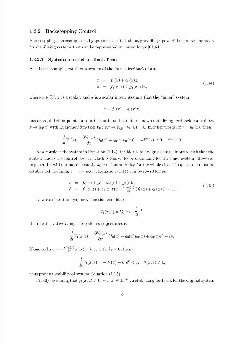
then the origin is Lyapunov stable. If in addition

∂V (x)

∂x f (x) < 0, (1.5)

the origin is asymptotically stable. Furthermore, if there exist positive constants α, β , such that

αx2 ≤ V (x) ≤ β x2, (1.6)

∂V (x)

∂x f (x) ≤ −V (x),

then the origin is exponentially stable.

The function V (x) is said to be a Lyapunov function of the dynamical system in Equation (1.2) if it

satisfies these conditions. Therefore, the problem of establishing stability of a dynamical system can

be reduced to that of finding a Lyapunov function for the system. If a system is stable, a Lyapunov

function is guaranteed to exist [36,58,118], although finding one may not be always straightforward.

It should be noted that the inability to find a Lyapunov function for a system does not imply its

instability. A Lyapunov function is said to be radially unbounded if as x → ∞, V (x) → ∞.

If a radially unbounded Lyapunov function exists for a dynamical system whose solution exists

globally, then the stability of that system can be established globally. In the following, V (x(t)) and∂V (x(t))

∂x(t) f (x(t)) are used interchangeably.

It is possible to relax the strict negative definiteness condition on the Lyapunov derivative in

Equation (1.5) if it can be shown that the Lyapunov function is non-increasing everywhere, and the

only trajectories where V (x) = 0 indefinitely is the origin of the system. This result is captured by

the Barbashin-Krasovskii-LaSalle invariance principle (see e.g. [36,58,118]), which provides sufficient

conditions for convergence of the solution of nonlinear dynamical system to its largest invariantset (described shortly). A point x p is said to be a positive limit point of the solution x(t) to

the nonlinear dynamical system of Equation (1.2) if there exists an infinite sequence {ti} such that

ti → +∞ and x(ti) → x p, as i → ∞. The positive limit set (also referred to as ω-limit set) is the set

of all positive limit points. A set M is said to be positively invariant if x(0) ∈ M then x(t) ∈ M for

all t ≥ 0. That is, a positively invariant set is the set of all initial conditions for which the solution

of Equation (1.2) does not leave the set. The set of all equilibriums of a nonlinear dynamical system

for example is a positively invariant set. The Barbashin-Krasovskii-LaSalle theorem can be stated

as follows:

Theorem 1.2.2 [36,58,118] Consider the dynamical system of Equation (1.2), and assume that D is a compact positively invariant set. Furthermore, assume that there exists a continuously

differentiable function V (x) : D → R+ such that ∂V (x)∂x f (x) ≤ 0 in D, and let M be the largest

invariant set contained in the set S = {x ∈ D|V (x) = 0}. Then, if x(0) in D, the solution x(t) of

the dynamical system approaches M as t → ∞.

A corollary to this theorem states that if V (x) is also positive definite over D and no solution

except the solution x(t) = 0 can stay in the set S , then the origin is asymptotically stable [36,58].

4



In the following the quaternion attitude controller discussed in “Linear Flight Control Tech-

niques for Unmanned Aerial Vehicles” is used to illustrate the application of Lyapunov stability

analysis. A unit quaternion

q = (q, q ), q 2 + q · q = 1,

can be interpreted as a representation of a rotation of an angle θ = 2 arccos(q ), around an axisparallel to q . The attitude dynamics of an airplane modeled as a rigid body with quaternion

attitude representation can be given by

J B ωB = −ωB × J BωB + u

q = 12q ◦ (0, ωB).

(1.7)

where J B is the inertia tensor expressed in the body frame, ωB = [ω1, ω2, ω3]T ∈ R3 is the angular

velocity of the body frame with respect to the inertial frame, and u is the control input. The

operator ◦ denotes the quaternion composition operator, using which the quaternion kinematics

equation 1.7 can be expanded as

q 1 ◦ (0, ωB) = (− q 1 · ωB, q 1ωB + q 1 q 1 + q 1 × ωB).

The goal is to design a control law u such that the system achieves the unique zero attitude

represented by the unit quaternions [1, 0, 0, 0] and [−1, 0, 0, 0]. It is shown that a control law of the

form

u = −q

2K p q − K dωB (1.8)

where K p and K d are positive definite gain matrices, guarantees that the system achieves zero

attitude using Lyapunov analysis. Consider the Lyapunov candidate

V (q, ω) = 1

2 q · K p q +

1

2ω · J ω.

Note that V (q, ω) ≥ 0, and is zero only at q = (±1, 0), ω = 0; both points correspond to the rigid

body at rest at the identity rotation. The time derivative of the Lyapunov candidate along the

trajectories of system Equation (1.7) under the feedback Equation (1.8) is computed as:

V (q, ω) = q · K p q + ω · J ω.

Note that from the kinematics of unit quaternions, q = 1/2 (qω + q × ω) . Then,

V (q, ω) = 1

2 q · K p (qω + q × ω) − ω ·

ω × Jω +

q

2K p q + K dω

= −ω · K dω ≤ 0.

Therefore, V (q, ω) ≤ 0, furthermore the set S = {x ∈ D|V (x) = 0} consists of only q = (±1, 0),

ω = 0. Therefore, Theorem 1.2.2 guarantees asymptotic convergence to this set.

5



1.3 Lyapunov Based Control

1.3.1 Gain Scheduling

In the companion chapter titled “Linear Flight Control Techniques for Unmanned Aerial Vehicles” it

was shown that aircraft dynamics can be linearized around equilibrium points (or trim conditions).A commonly used approach in aircraft control leverages this fact by designing a finite number

of linear controllers, each corresponding to a linear model of the aircraft dynamics near a design

trim condition. The key motivation in this approach is to leverage well understood tools in linear

systems design. Let Ai, Bi, i ∈ {1, . . . , N } denote the matrices containing the aerodynamic and

control effectiveness derivatives around the ith trimmed condition xi. Let X 1, . . . , X N be a partition

of the state space, i.e., ∪N i=1X i = R

n, X i ∩ X j = ∅ for i = j , into regions that are “near” the design

trim conditions; in other words, whenever the state x is in the region X i, the aircraft dynamics

are approximated by the linearization at xi ∈ X i. Then, the dynamics of the aircraft can be

approximated as a state-dependent switching linear system as follows

x = Aix + Biu when x ∈ X i. (1.9)

The idea in gain scheduling based control is to create a set of gains K i corresponding to each of

the switched model and apply the linear control u = K ix. Contrary to intuition, however, simply

ensuring that the ith system is rendered stable (that is, the real parts of the eigenvalues of Ai −BiK i

are negative) is not sufficient to guarantee the closed loop stability of Equation (1.9) [12,77,78]. A

Lyapunov based approach can be used to guarantee the stability of the closed-loop when using gain

scheduling controller.

Consider the following Lyapunov candidate

V (x(t)) = x(t)T P x(t), (1.10)

where P is a positive definite matrix, that is, for all x = 0, xT P x > 0. Therefore, V (0) = 0, and

V (x) > 0 for all x = 0 making V a valid Lyapunov candidate. The derivative of the Lyapunov

candidate is

V (x) = xT P x + xT P x. (1.11)

For the ith system, Equation (1.11) can be written as

V (x) = (Aix − BiK ix)T P x + xT P (Aix − BiK ix). (1.12)

Let Ai = (Ai − BiK i), then from Lyapunov theory it follows that for a positive definite matrix Q

if for all i

AT i P + P Ai < −Q, (1.13)

∂V (x)∂x f (x) < −xT Qx. In this case, V (x) is a common Lyapunov function for the switched closed

6



UAV Dynamicsf (x)

ControlSelector

linear control 1linear control 2

linear control 3

linear control 4

xu

Figure 1.2: Schematic of a gain scheduled scheme for UAV control. The controller selector boxdecides which linear controller is to be used based on measured system states. In the depictedsituation, controller 1 is active.

loop system (see e.g. [77]) establishing the stability of the equilibrium at the origin. Therefore,

the control design task is to select the gains K i such that Equation (1.13) is satisfied. One way to

tackle this problem is through the framework of Linear Matrix Inequalities (LMI) [10,33]. It should

be noted that the condition in Equation (1.13) allows switching between the linear models to occur

infinitely fast, this can be a fairly conservative assumption for most UAV control applications. This

condition can be relaxed to AT i P i +P i Ai < −Qi for Qi > 0 to guarantee the stability of the system if

the system does not switch arbitrarily fast. A rigorous condition for proving asymptotic stability of

a system of the form 1.9 was introduced in [12]. Let V i, i ∈ {1, . . . , N } be Lyapunov-like functions,

i.e., positive definite functions such that V i(x) < 0 whenever x ∈ X i \ {0}. Define V i[k] as the

infimum of all the values taken by V i during the k-th time interval over which x ∈ X i. Then, if the

system satisfies the sequence non-increasing condition V i[k + 1] < V i[k], for all k ∈ N, asymptotic

stability is guaranteed [12,77].

The above example illustrates the use of Lyapunov techniques in synthesizing controllers. In

general, given the system of equation 1.2, and a positive definite Lyapunov candidate, the Lyapunov

synthesis approach to create robust exponentially stable controllers can be summarized as follows:

Let V (x) = g(x, u), find a control function u(x) such that V (x) < −V (x) for some positive constant

. Robust methods for Lyapunov based control synthesis are discussed in [36]. Furthermore, [111]

provides an output feedback control algorithms for system with switching dynamics.

The framework of Linear Parameter Varying (LPV) systems lends naturally to design andanalysis of controllers based on a UAV dynamics representation via linearization across multiple

equilibria. Gain scheduling based LPV control synthesis techniques have been studied for flight

control and conditions for stability have been established (see e.g. [7,40,69,84,115]).

7



1.3.2 Backstepping Control

Backstepping is an example of a Lyapunov based technique, providing a powerful recursive approach

for stabilizing systems that can be represented in nested loops [61,64].

1.3.2.1 Systems in strict-feedback form

As a basic example, consider a system of the (strict-feedback) form

x = f 0(x) + g0(x)z,

z = f 1(x, z) + g1(x, z)u,(1.14)

where x ∈ Rn, z is a scalar, and u is a scalar input. Assume that the “inner” system

x = f 0(x) + g0(x)z,

has an equilibrium point for x = 0, z = 0, and admits a known stabilizing feedback control lawx → u0(x) with Lyapunov function V 0 : Rn → R≥0, V 0(0) = 0. In other words, if z = u0(x), then

d

dtV 0(x) =

∂V 0(x)

∂x (f 0(x) + g0(x)u0(x)) = −W (x) < 0, ∀x = 0.

Now consider the system in Equation (1.14), the idea is to design a control input u such that the

state z tracks the control law u0, which is known to be stabilizing for the inner system. However,

in general z will not match exactly u0(x), thus stability for the whole closed-loop system must be

established. Defining e = z − u0(x), Equation (1.14) can be rewritten as

x = f 0(x) + g0(x)u0(x) + g0(x)e,

e = f 1(x, z) + g1(x, z)u − ∂ u0(x)∂x (f 0(x) + g0(x)z) = v.

(1.15)

Now consider the Lyapunov function candidate

V 1(x, e) = V 0(x) + 1

2e2;

its time derivative along the system’s trajectories is

d

dt

V 1(x, e) = ∂V 0(x)

∂x

(f 0(x) + g0(x)u0(x) + g0(x)e) + ev.

If one picks v = − ∂V 0(x)∂x g0(x) − k1e, with k1 > 0, then

d

dtV 1(x, e) = −W (x) − k1e2 < 0, ∀(x, e) = 0,

thus proving stability of system Equation (1.15).

Finally, assuming that g1(x, z) = 0, ∀(x, z) ∈ Rn+1, a stabilizing feedback for the original system

8



in Equation (1.14) can be recovered as

u(x, z) = 1

g1(x, z)

∂ u0(x)

∂x (f 0(x) + g0(x)z) − f 1(x, z) + v

= 1

g1(x, z)∂ u0(x)

∂x (f 0(x) + g0(x)z) − f 1(x, z) −

∂ V 0(x)

∂x g0(x) − k1(z − u0(x)) . (1.16)

Since the control law in Equation (1.16) stabilizes system Equation (1.14), with Lyapunov function

V 1, a similar argument can be used to recursively build a control law for a system in strict-feedback

form of arbitrary order,

x = f 0(x) + g0(x) z1,

z1 = f 1(x, z1) + g1(x, z1) z2,...

zm = f m(x, z1, . . . , zm) + g1(x, zm) u,

(1.17)

The procedure is summarized as follows: start from the “inner” system, for which a stabilizingcontrol law and a Lyapunov function are known. Define an error between the known control law

and the actual input to the inner system. Augment the Lyapunov function with the square of

the error. Design a new control law that ensures the stability of the augmented system. Repeat

using the augmented system just defined as the new inner system. This recursion, “stepping back”

from the inner system all the way to the control input gives the name to the method. A detailed

description of control synthesis for small unmanned helicopters using backstepping techniques is

provided in [106].

1.3.3 Model Predictive Control (MPC)

MPC has been successfully used for many years in industrial applications with relatively slow

dynamics (e.g., chemical reactions [55,82,86]), it is only in the past decade that the computational

power been available to enable online optimization for fast system dynamics typical in aerospace

applications (early relevant demonstrations are in [27–29,83,108,110]). MPC attempts to solve the

following problem: Design an admissible piecewise continuous control input u(t) that guarantees

the system behaves like a reference model without violating the given state and input constraints.

As such, a key benefit MPC is the ability to optimize the control input in the presence of state and

input constraints. Furthermore, because MPC explicitly considers the operating constraints, it can

operate closer to hard constraint boundaries than traditional control schemes.

MPC can be formulated using several types of cost function, however, due to the availability

of robust quadratic solvers, the following formulation is popular. Find the optimal control u(t)

such that for given positive (semi) definite matrices Q, R, and S , the following quadratic cost is

minimized

J ∞(e, u) =

∞t0

eT (t)Qe(t) + uT (t)Ru(t)dt, x ∈ Ξ, u ∈ Π. (1.18)

In the presence of constraints, a closed form solution for an infinite horizon optimization problem

9



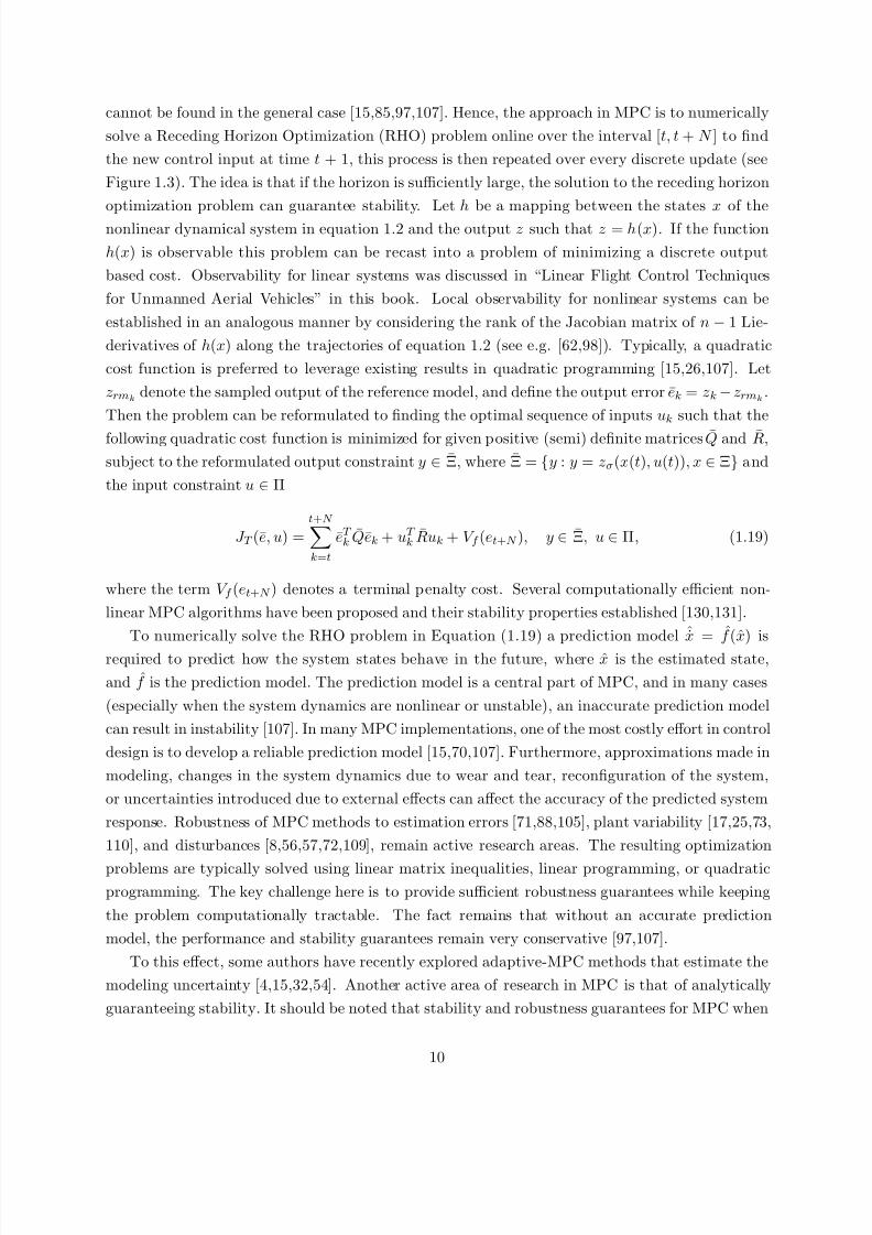
cannot be found in the general case [15,85,97,107]. Hence, the approach in MPC is to numerically

solve a Receding Horizon Optimization (RHO) problem online over the interval [ t, t + N ] to find

the new control input at time t + 1, this process is then repeated over every discrete update (see

Figure 1.3). The idea is that if the horizon is sufficiently large, the solution to the receding horizon

optimization problem can guarantee stability. Let h be a mapping between the states x of the

nonlinear dynamical system in equation 1.2 and the output z such that z = h(x). If the function

h(x) is observable this problem can be recast into a problem of minimizing a discrete output

based cost. Observability for linear systems was discussed in “Linear Flight Control Techniques

for Unmanned Aerial Vehicles” in this book. Local observability for nonlinear systems can be

established in an analogous manner by considering the rank of the Jacobian matrix of n − 1 Lie-

derivatives of h(x) along the trajectories of equation 1.2 (see e.g. [62,98]). Typically, a quadratic

cost function is preferred to leverage existing results in quadratic programming [15,26,107]. Let

zrmk denote the sampled output of the reference model, and define the output error ek = zk − zrmk

.

Then the problem can be reformulated to finding the optimal sequence of inputs uk such that the

following quadratic cost function is minimized for given positive (semi) definite matrices Q and R,

subject to the reformulated output constraint y ∈ Ξ, where Ξ = {y : y = zσ(x(t), u(t)), x ∈ Ξ} and

the input constraint u ∈ Π

J T (e, u) =t+N k=t

eT k

Qek + uT k

Ruk + V f (et+N ), y ∈ Ξ, u ∈ Π, (1.19)

where the term V f (et+N ) denotes a terminal penalty cost. Several computationally efficient non-

linear MPC algorithms have been proposed and their stability properties established [130,131].

To numerically solve the RHO problem in Equation (1.19) a prediction model ˆx = f (x) is

required to predict how the system states behave in the future, where x is the estimated state,

and f is the prediction model. The prediction model is a central part of MPC, and in many cases

(especially when the system dynamics are nonlinear or unstable), an inaccurate prediction model

can result in instability [107]. In many MPC implementations, one of the most costly effort in control

design is to develop a reliable prediction model [15,70,107]. Furthermore, approximations made in

modeling, changes in the system dynamics due to wear and tear, reconfiguration of the system,

or uncertainties introduced due to external effects can affect the accuracy of the predicted system

response. Robustness of MPC methods to estimation errors [71,88,105], plant variability [17,25,73,

110], and disturbances [8,56,57,72,109], remain active research areas. The resulting optimization

problems are typically solved using linear matrix inequalities, linear programming, or quadraticprogramming. The key challenge here is to provide sufficient robustness guarantees while keeping

the problem computationally tractable. The fact remains that without an accurate prediction

model, the performance and stability guarantees remain very conservative [97,107].

To this effect, some authors have recently explored adaptive-MPC methods that estimate the

modeling uncertainty [4,15,32,54]. Another active area of research in MPC is that of analytically

guaranteeing stability. It should be noted that stability and robustness guarantees for MPC when

10



UAV Dynamics: f

ModelPredictorRecedingHorizonOptimizer

MPC

Predicted states

Candidate control input

xu

External Commands

Figure 1.3: Schematic of a model predictive controller which minimizes a quadratic cost over afinite horizon

the system dynamics are linear are at least partially in place [15]. With an appropriate choice of

V f (et+N ) and with terminal inequality state and input constraints (and in some cases without) sta-bility guarantees for nonlinear MPC problems have been established [79,97,129]. However, due to

the open loop nature of the optimization strategy, and dependence on the prediction model, guar-

anteeing stability and performance for a wide class of nonlinear systems still remains an active area

of research. A challenge in implementing MPC methods is to ensure that the optimization problem

can be solved in real-time. While several computationally efficient nonlinear MPC strategies have

been devised, ensuring that a feasible solution is obtained in face of processing and memory con-

straints remains an active challenge for MPC application on UAVs, where computational resources

are often constrained [121].

1.3.4 Model Inversion Based Control

1.3.4.1 Dynamic Model Inversion using Differentially Flat Representation of Aircraft

Dynamics

A complete derivation of the nonlinear six degree of freedom UAV dynamics was presented in

“Linear Flight Control Techniques for Unmanned Aerial Vehicles” in this book. For trajectory

tracking control using feedback linearization, simpler representations of UAV dynamics are often

useful. One such representation is the differentially flat representation (see e.g. [39]). The dynamical

system in Equation (1.1) with output y = h(x, u) is said to be differentially flat with flat output

z if there exists a function g such that the state and input trajectories can be represented as afunction of the flat output and a finite number of its derivatives:

(x, u) = g

y, y, y, ...,

dny

dtn

. (1.20)

In the following, assume that a smooth reference trajectory pd is given for a UAV in the inertial

frame (see “Linear Flight Control Techniques for Unmanned Aerial Vehicles” in this book), and

11



that the reference velocity ˙ pd and reference acceleration ¨ pd can be calculated using the reference

trajectory. Consider the case of a conventional fixed wing UAV that must be commanded a forward

speed to maintain lift, hence ˙ pd = 0. A right handed orthonormal frame of reference wind axes

can now be defined by requiring that the desired velocity vector is aligned with the xW axis of the

wind axis (see “Linear Flight Control Techniques for Unmanned Aerial Vehicles” in this book for

details), and the lift and drag forces are in the xW –zW plane of the wind axis the zW axis such

that there are no side forces. The acceleration can be written as

¨ pd = g + f I /m, (1.21)

where f I is the sum of propulsive and aerodynamic forces on the aircraft in the inertial frame. Let

RIW denote the rotation matrix that transports vectors from the defined wind reference frame to

the inertial frame. Then

¨ pd = g + RIW aW , (1.22)

where aW is the acceleration in the wind frame. Let ω = [ω1, ω2, ω3]T denote the angular velocity

in the wind frame; then the above equation can be differentiated to obtain

d3 pd

dt3 = RIW (ω × aW ) + RIW aW , (1.23)

by using the relationship RIW aW = RIW ωaW = RIW (ω × aW ) (see Section 1.2.2 of “Linear Flight

Control Techniques for Unmanned Aerial Vehicles” in this book). Let at denote the tangential

acceleration along the xW direction, an denote the normal acceleration along the zW direction,

and V denote the forward speed. Furthermore, let e1 = [1, 0, 0]T . Then in coordinated flight

˙ pd = V RIW e1, hence¨ pd = V RIW e1 + V RIW (ω × e1). (1.24)

Combining equation 1.22 and equation 1.24 the following relationship can be formed

¨ pd = RIW

V

V ω3

−V ω2

. (1.25)

Equation 1.25 allows the desired ω2 and ω3 to be calculated from the desired acceleration ¨ pd.

Furthermore, from equation 1.23

at

ω1

an

=

−ω2an

ω3at/n

ω2at

+

1 0 0

0 −1/an 0

0 0 1

RT

IW

d3 pd

dt3 . (1.26)

The above equation defines a differentially flat system of aircraft dynamics with flat output pd

and inputs [at, ω1, an], if V = ˙ pd = 0 (nonzero forward speed) and an = 0 (nonzero normal

12



acceleration). The desired tangential and normal accelerations required to track the path pd can

be controlled through the thrust T (δ T ) which is a function of the throttle input δ T , the lift L(α),

and the drag D(α) which are functions of the angle of attack α by noting that in the wind axes

at = T (δ T )cos α − D(α), (1.27)

an = −T (δ T )sin α − L(α).

To counter any external disturbances that cause trajectory deviation, a feedback term can be added.

Let p be the actual position of the aircraft, u be the control input, and consider a system in whichd3 pddt3 = u:

d

dt

p

˙ p

¨ p

=

0 1 0

0 0 1

0 0 0

p

˙ p

¨ p

+

0

0

1

u. (1.28)

Defining e = p − pd the above equation can be written in terms of the error

d

dt

e

e

e

=

0 1 0

0 0 1

0 0 0

e

e

e

+

0

0

1

u −

d3 pd

dt3

. (1.29)

Therefore, letting u = d3 pdt3

−K

e e eT

where K is the stabilizing gain, and computing at, an, ω1

from ( p, ˙ p, ¨ p, u) guarantees asymptotic closed loop stability of the system (see [39] for further detail

of the particular approach presented). This approach is essentially that of feedback linearization

and dynamic model inversion, which is explored in the general setting in the next section.

1.3.4.2 Approximate Dynamic Model Inversion

The idea in approximate dynamic inversion based controllers is to use a (approximate) dynamic

model of the UAV to assign control inputs based on desired angular rates and accelerations. Let

x(t) = [xT 1 (t), xT

2 (t)]T ∈ Rn be the known state vector, with x1(t) ∈ R

n2 and x2(t) ∈ Rn2 , let

u(t) ∈ Rn2 denote the control input, and consider the following multiple-input nonlinear uncertain

dynamical system

x1(t) = x2(t) (1.30)

x2(t) = f (x(t), u(t)),

where the function f is assumed to be known and globally Lipschitz continuous, and control input

u is assumed to be bounded and piecewise continuous. These conditions are required to ensure

the existence and uniqueness of the solution to Equation (1.30). Furthermore, a condition on

controllability of f with respect to u must also be assumed. Note also the requirement on as

many control inputs as the number of states directly affected by the input (x2). For UAV control

13



problem this assumption can usually be met through the successive loop closure approach (see

“Linear Flight Control Techniques for Unmanned Aerial Vehicles” in this book). For example, for

fixed wing control aileron, elevator, rudder, and throttle control directly affect roll, pitch, yaw rate,

and velocity. This assumption can also met for rotorcraft UAV velocity control with the attitudes

acting as virtual inputs for velocity dynamics, and the three velocities acting as virtual inputs for

the position dynamics [49].

In dynamic model inversion based control the goal is to find the desired acceleration, referred

to as the pseudo-control input ν (t) ∈ Rn2, which can be used to find the control input u such that

the system states track the output of a reference model. Let z = (x, u), if the exact system model

f (z) in Equation (1.30) is invertible, for a given ν (t), u(t) can be found by inverting the system

dynamics. However, since the exact system model is usually not invertible, let ν be the output of

an approximate inversion model f such that ν = f (x, u) is continuous and invertible with respect

to u, that is, the operator f −1 : Rn+n2 → Rl exists and assigns for every unique element of Rn+n2

a unique element of Rl. An approximate inversion model that satisfies this requirement is required

to guarantee that given a desired pseudo-control input ν ∈ Rn2 a control command u can be found

by dynamic inversion as follows

u = f −1(x, ν ). (1.31)

The model in Section 1.3.4.1 is an example of a differentially flat approximate inversion model.

For the general system in Equation (1.30), the use of an approximate inversion model results in a

model error of the form

x2 = ν + ∆(x, u) (1.32)

where ∆ is the modeling error. The modeling error captures the difference between the system

dynamics and the approximate inversion model

∆(z) = f (z) − f (z). (1.33)

Note that if the control assignment function were known and invertible with respect to u, then an

inversion model can be chosen such that the modeling error is only a function of the state x.

Often, UAV dynamics can be represented by models that are affine in control. In this case

the existence of the approximate inversion model can be related directly to the invertibility of the

control effectiveness matrix B (e.g., see [50]). For example, let G ∈ Rn2×n2, and let B ∈ R

n2×l

denote the control assignment matrix and consider the following system

x1(t) = x2(t) (1.34)

x2(t) = Gx2(t) + B(Θ(x) + u(t)),

where Θ(x) is a nonlinear function. If BT B is invertible, and the pair (G, B) is controllable,

one approximate inversion model is: ν (t) = Bu(t), which results in a unique u for a unique ν :

u(t) = (BT B)−1BT ν (t). Adding and subtracting ν = Bu yields Equation (1.32), with ∆(x) =

14



Gx2 + B(Θ(x) + u) − Bu = Gx2 + BΘ(x).

A reference model is used to characterize the desired response of the system

x1rm = x2rm , (1.35)

x2rm = f rm(xrm, r),

where f rm(xrm(t), r(t)) denote the reference model dynamics which are assumed to be continuously

differentiable in xrm for all xrm ∈ Dx ⊂ Rn. The command r(t) is assumed to be bounded and

piecewise continuous, furthermore, f rm is assumed to be such that xrm is bounded for a bounded

reference input.

The pseudo-control input ν is designed by combining a linear feedback part ν pd = [K 1, K 2]e

with K 1 ∈ Rn2×n2 and K 2 ∈ R

n2×n2, a linear feedforward part ν rm = x2rm , and an approximate

feedback linearizing part ν ai(z)

ν = ν rm + ν pd − ν ai. (1.36)

Defining the tracking error e as e(t) = xrm(t) − x(t), and using Equation (1.32) the tracking

error dynamics can be written as

e = xrm −

x2

ν + ∆

. (1.37)

Letting A =

0 I 1

−K 1 −K 2

, B = [0, I 2]T where 0 ∈ R

n2×n2, I 1 ∈ Rn2×n2, and I 2 ∈ R

n2×n2 are the

zero and identity matrices, and using Equation (1.36) gives the following tracking error dynamics

that are linear in e

e = Ae + B[ν ai(z) − ∆(z)]. (1.38)

The baseline linear full state feedback controller ν pd should be chosen such that A is a Hurwitz

matrix. Furthermore, letting ν ai = ∆(z) using Equation (1.33) ensures that the above tracking

error dynamics is exponentially stable, and the states of the UAV track the reference model.

1.3.5 Model Reference Adaptive Control

The Model Reference Adaptive (MRAC) Control architecture has been widely studied for UAV

control in presence of nonlinearities and modeling uncertainties (see e.g. [49,66,96,102]). MRAC

attempts to ensure that the controlled states track the output of an appropriately chosen reference

model (see e.g. [6,44,92,122]). Most MRAC methods achieve this by using a parameterized modelof the uncertainty, often referred to as the adaptive element and its parameters referred to as

adaptive weights. Aircraft dynamics can often be separated into a linear part whose mathematical

model is fairly well known, and an uncertain part that may contain unmodeled linear or nonlinear

effects. This representation is also helpful in representing nonlinear external disturbances affecting

the system dynamics. Therefore, one typical technique for implementing adaptive controllers is to

augment a baseline linear controller, designed and verified using techniques discussed in “Linear

15



Reference

Model

(Approximate)Inversion

model f −1

UAVdynamics f

u

Feedbacklinearizer

PD compensator

r(t) ν rm ν x −

e

ν pd

ν ai

xrm

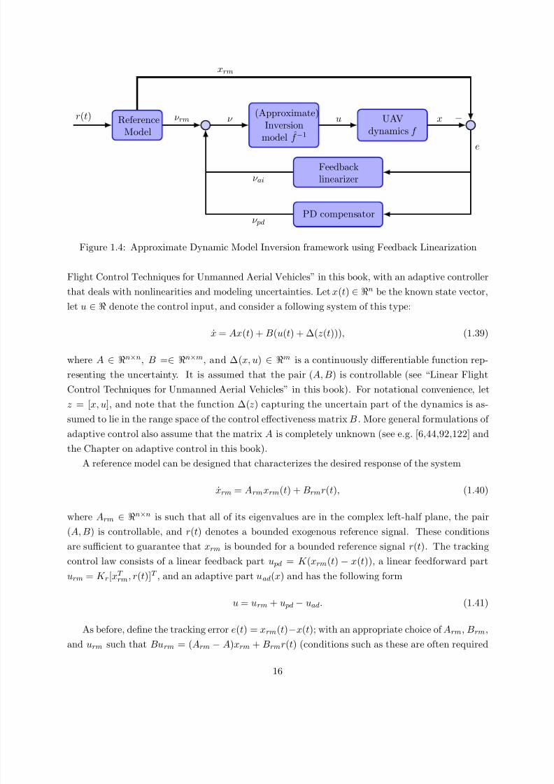
Figure 1.4: Approximate Dynamic Model Inversion framework using Feedback Linearization

Flight Control Techniques for Unmanned Aerial Vehicles” in this book, with an adaptive controller

that deals with nonlinearities and modeling uncertainties. Let x(t) ∈ n be the known state vector,

let u ∈ denote the control input, and consider a following system of this type:

x = Ax(t) + B(u(t) + ∆(z(t))), (1.39)

where A ∈ n×n, B =∈ n×m, and ∆(x, u) ∈ m is a continuously differentiable function rep-

resenting the uncertainty. It is assumed that the pair (A, B) is controllable (see “Linear Flight

Control Techniques for Unmanned Aerial Vehicles” in this book). For notational convenience, let

z = [x, u], and note that the function ∆(z) capturing the uncertain part of the dynamics is as-

sumed to lie in the range space of the control effectiveness matrix B . More general formulations of

adaptive control also assume that the matrix A is completely unknown (see e.g. [6,44,92,122] and

the Chapter on adaptive control in this book).

A reference model can be designed that characterizes the desired response of the system

xrm = Armxrm(t) + Brmr(t), (1.40)

where Arm ∈ n×n is such that all of its eigenvalues are in the complex left-half plane, the pair

(A, B) is controllable, and r(t) denotes a bounded exogenous reference signal. These conditions

are sufficient to guarantee that xrm is bounded for a bounded reference signal r(t). The trackingcontrol law consists of a linear feedback part u pd = K (xrm(t) − x(t)), a linear feedforward part

urm = K r[xT rm, r(t)]T , and an adaptive part uad(x) and has the following form

u = urm + u pd − uad. (1.41)

As before, define the tracking error e(t) = xrm(t)−x(t); with an appropriate choice of Arm, Brm,

and urm such that Burm = (Arm − A)xrm + Brmr(t) (conditions such as these are often required

16



in MRAC and are referred to as matching conditions ), the tracking error dynamics simplify to

e = Ame + B(uad(x, u) − ∆(x, u)), (1.42)

where the baseline full state feedback controller u pd = Kx is assumed to be designed such that

Am = A − BK is a Hurwitz matrix. Hence for any positive definite matrix Q ∈ n×n , a positive

definite solution P ∈ n×n exists to the Lyapunov equation

AT mP + P Am = −Q. (1.43)

MRAC architecture is depicted in Figure 1.5. Several MRAC approaches [6,16,44,67,92,122]

assume that the uncertainty ∆(z) can be linearly parameterized, that is, there exist a vector of

constants W = [w1, w2,....,wm]T and a vector of continuously differentiable functions Φ(z) =

[φ1(z), φ2(z),....,φm(z)]T such that

∆(z) = W ∗T Φ(z). (1.44)

The case when the basis of the uncertainty is known, that is the basis Φ(x) is known, has been

referred to as the case of structured uncertainty [18]. In this case letting W denote the estimate W ∗

the adaptive element is chosen as uad(x) = W T Φ(x). For this case it is known that the adaptive

law

W = −ΓW Φ(z)eT P B (1.45)

where ΓW is a positive definite learning rate matrix results in e(t) → 0. However, it should be noted

that Equation (1.50) does not guarantee the convergence (or even the boundedness) of W [91,122].

A necessary and sufficient condition for guaranteeing W (t) → W is that Φ(t) be persistently exciting

(PE) [11,44,92,122].

Several approaches have been explored to guarantee boundedness of the weights without need-

ing PE, these include the classic σ-modification [44], the e-modification [92],and projection based

adaptive control [122]. Let κ denote the σ modification gain, then the σ-modification adaptive law

is

W = −ΓW

Φ(z(t))eT P B + κW

. (1.46)

Thus it can be seen that the goal of σ modification is to add damping to the weight evolution. In

e modification, this damping is scaled by the norm of the error e. It should be noted that these

adaptive laws guarantee the boundedness of the weights, however, they do not guarantee that the

weights converge to their true values without PE.

A concurrent learning approach introduced in [18] guarantees exponential tracking error and

weight convergence by concurrently using recorded data with current data without requiring PE.

Other approaches that use recorded data include the Q-modification approach that guarantees

convergence of the weights to a hyperplane where the ideal weights are contained [124], and the

retrospective cost optimization approach [113]. Other approaches to MRAC favor instantaneous

domination of uncertainty over weight convergence, one such approach is L1 adaptive control [16,42].

17



Several other approaches to MRAC also exist, including the composite adaptive control approach in

which direct and indirect adaptive control are combined [67], the observer based reference dynamics

modification in adaptive controllers in which transient performance is improved by drawing on

parallels between the reference model and a Luenberger observer [68]. The derivative-free MRAC in

which a discrete derivative free update law is used in a continuous framework [127] and the optimal

control modification [95]. Among approaches that deal with actuator time delays and constraints

include the adaptive loop recovery modification which recovers nominal reference model dynamics

in presence of time delays [13], and the pseudo control hedging which allows adaptive controllers

to be implemented in presence of saturation [51].

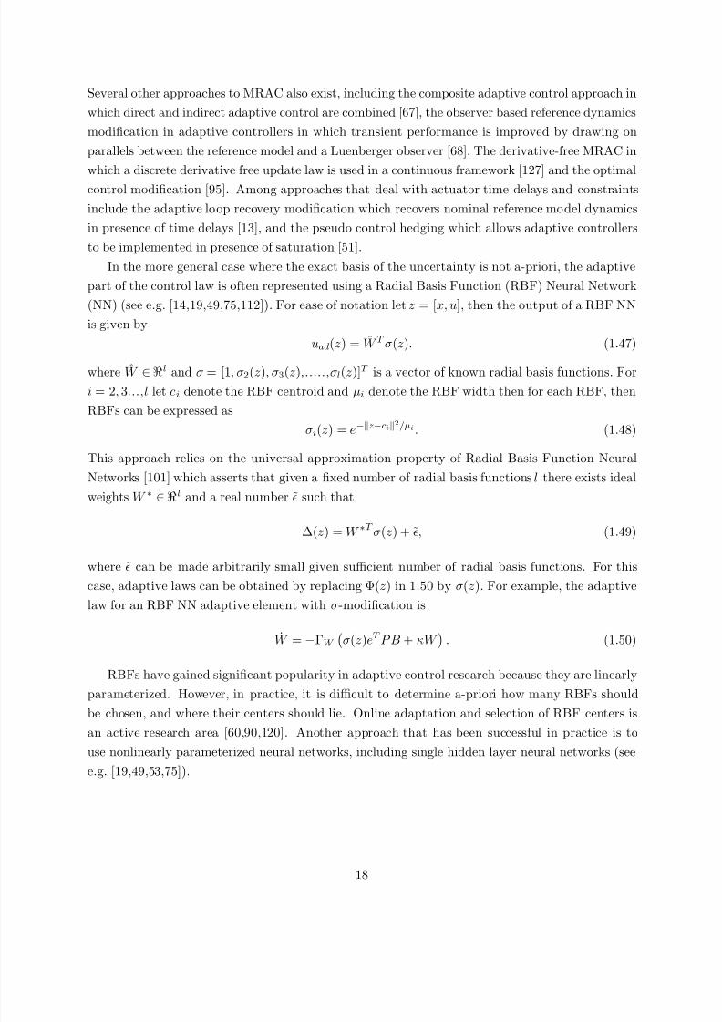
In the more general case where the exact basis of the uncertainty is not a-priori, the adaptive

part of the control law is often represented using a Radial Basis Function (RBF) Neural Network

(NN) (see e.g. [14,19,49,75,112]). For ease of notation let z = [x, u], then the output of a RBF NN

is given by

uad(z) = W T σ(z). (1.47)

where W ∈ l and σ = [1, σ2(z), σ3(z),.....,σl(z)]T is a vector of known radial basis functions. For

i = 2, 3...,l let ci denote the RBF centroid and µi denote the RBF width then for each RBF, then

RBFs can be expressed as

σi(z) = e−z−ci2/µi . (1.48)

This approach relies on the universal approximation property of Radial Basis Function Neural

Networks [101] which asserts that given a fixed number of radial basis functions l there exists ideal

weights W ∗ ∈ l and a real number such that

∆(z) = W

∗T

σ(z) + , (1.49)

where can be made arbitrarily small given sufficient number of radial basis functions. For this

case, adaptive laws can be obtained by replacing Φ(z) in 1.50 by σ(z). For example, the adaptive

law for an RBF NN adaptive element with σ-modification is

W = −ΓW

σ(z)eT P B + κW

. (1.50)

RBFs have gained significant popularity in adaptive control research because they are linearly

parameterized. However, in practice, it is difficult to determine a-priori how many RBFs should

be chosen, and where their centers should lie. Online adaptation and selection of RBF centers isan active research area [60,90,120]. Another approach that has been successful in practice is to

use nonlinearly parameterized neural networks, including single hidden layer neural networks (see

e.g. [19,49,53,75]).

18



ReferenceModel

UAV dynamicsAx + B(u + ∆(x, u))

Adaptivecontroller

PD compensator

r(t) urm u x −

e

u pd

uad

xrm

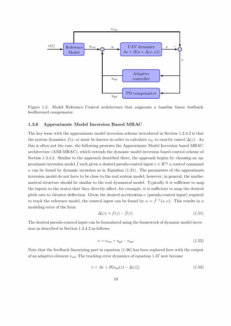
Figure 1.5: Model Reference Control architecture that augments a baseline linear feedback-

feedforward compensator

1.3.6 Approximate Model Inversion Based MRAC

The key issue with the approximate model inversion scheme introduced in Section 1.3.4.2 is that

the system dynamics f (x, u) must be known in order to calculate ν ai to exactly cancel ∆(z). As

this is often not the case, the following presents the Approximate Model Inversion based MRAC

architecture (AMI-MRAC), which extends the dynamic model inversion based control scheme of

Section 1.3.4.2. Similar to the approach described there, the approach begins by choosing an ap-

proximate inversion model f such given a desired pseudo-control input ν ∈ Rn2 a control command

u can be found by dynamic inversion as in Equation (1.31). The parameters of the approximateinversion model do not have to be close to the real system model, however, in general, the mathe-

matical structure should be similar to the real dynamical model. Typically it is sufficient to map

the inputs to the states that they directly affect, for example, it is sufficient to map the desired

pitch rate to elevator deflection. Given the desired acceleration ν (pseudo-control input) required

to track the reference model, the control input can be found by u = f −1(x, ν ). This results in a

modeling error of the form

∆(z) = f (z) − f (z). (1.51)

The desired pseudo-control input can be formulated using the framework of dynamic model inver-

sion as described in Section 1.3.4.2 as follows:

ν = ν rm + ν pd − ν ad. (1.52)

Note that the feedback linearizing part in equation (1.36) has been replaced here with the output

of an adaptive element ν ad. The tracking error dynamics of equation 1.37 now become

e = Ae + B[ν ad(z) − ∆(z)]. (1.53)

19



Reference

Model

(Approximate)Inversion

model: f −1

UAVDynamics: f

u

Adaptivecontroller

PD compensator

r(t) ν rm x −

e

ν pd

ν ad

xrm

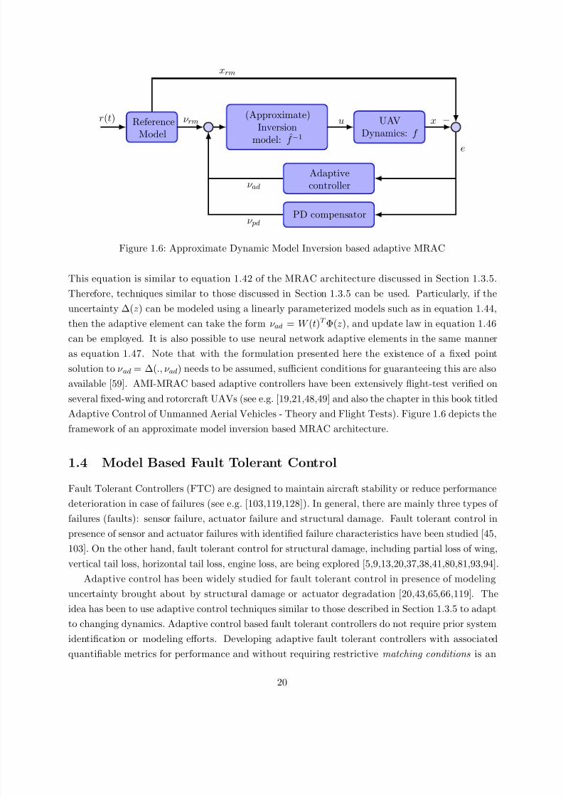
Figure 1.6: Approximate Dynamic Model Inversion based adaptive MRAC

This equation is similar to equation 1.42 of the MRAC architecture discussed in Section 1.3.5.Therefore, techniques similar to those discussed in Section 1.3.5 can be used. Particularly, if the

uncertainty ∆(z) can be modeled using a linearly parameterized models such as in equation 1.44,

then the adaptive element can take the form ν ad = W (t)T Φ(z), and update law in equation 1.46

can be employed. It is also possible to use neural network adaptive elements in the same manner

as equation 1.47. Note that with the formulation presented here the existence of a fixed point

solution to ν ad = ∆(., ν ad) needs to be assumed, sufficient conditions for guaranteeing this are also

available [59]. AMI-MRAC based adaptive controllers have been extensively flight-test verified on

several fixed-wing and rotorcraft UAVs (see e.g. [19,21,48,49] and also the chapter in this book titled

Adaptive Control of Unmanned Aerial Vehicles - Theory and Flight Tests). Figure 1.6 depicts theframework of an approximate model inversion based MRAC architecture.

1.4 Model Based Fault Tolerant Control

Fault Tolerant Controllers (FTC) are designed to maintain aircraft stability or reduce performance

deterioration in case of failures (see e.g. [103,119,128]). In general, there are mainly three types of

failures (faults): sensor failure, actuator failure and structural damage. Fault tolerant control in

presence of sensor and actuator failures with identified failure characteristics have been studied [45,

103]. On the other hand, fault tolerant control for structural damage, including partial loss of wing,

vertical tail loss, horizontal tail loss, engine loss, are being explored [5,9,13,20,37,38,41,80,81,93,94].

Adaptive control has been widely studied for fault tolerant control in presence of modeling

uncertainty brought about by structural damage or actuator degradation [20,43,65,66,119]. The

idea has been to use adaptive control techniques similar to those described in Section 1.3.5 to adapt

to changing dynamics. Adaptive control based fault tolerant controllers do not require prior system

identification or modeling efforts. Developing adaptive fault tolerant controllers with associated

quantifiable metrics for performance and without requiring restrictive matching conditions is an

20



open area of research. Alternatively, a model based approach can also be used for fault tolerant

control. An overview of one such approach is presented here.

1.4.1 Control Design for Maximum Tolerance Range using Model Based Fault

Tolerant Control

Fault tolerant control technique presented here is applicable to aircraft with possible damage that

lies approximately in the body x − z plane of symmetry, in other words vertical tail-damage as

illustrated in Figure 1.7. A linear model of aircraft dynamics was derived in “Linear Flight Control

Techniques for Unmanned Aerial Vehicles” in this book. In that model A represents the matrix

containing aerodynamic derivatives, and B represents the matrix containing the control effectiveness

derivatives. The states of the model considered here are x(t) = [u,w,q,θ,v,p,r,φ]T , and the

input given by u(t) = [δe,δf,δa,δr]T (see “Linear Flight Control Techniques for Unmanned Aerial

Vehicles” in this book for definitions of these variables, details of the corresponding A and B

matrices can be found in [76]). Variation to aerodynamic derivatives due to structural damage isapproximately proportional to the percentage of loss in structure [114]. Therefore, the linearized

motion of the damaged aircraft can be represented by a parameter-dependent model based on the

baseline linear model of the aircraft, where the parameters provide a notion of the degree of damage:

x(t) = (A − µ A)x(t) + (B − µ B)u(t), µ ∈ [0, 1] (1.54)

where µ is the parameter representing the damage degree . Specifically, µ = 0 represents the case of

no damage, µ = 1 represents complete tail loss, and 0 < µ < 1 represents partial vertical tail loss.

The damage loss can be related to a maximum change in the aerodynamic derivatives (e.g. ∆ C yβ )

and control effectiveness derivatives (e.g. ∆C yδr ) under damage in the following way:

∆C yβ ∆C nβ ∆C lβ∆C yp ∆C np ∆C lp∆C yr ∆C nr ∆C lr∆C yδr ∆C nδr ∆C lδr

= µ

∆C maxyβ

∆C maxnβ

∆C maxlβ

∆C maxyp ∆C max

np ∆C maxlp

∆C maxyr ∆C max

nr ∆C maxlr

∆C maxyδr

∆C maxnδr

∆C maxlδr

(1.55)

For a given linear controller gain K , let J (K, µ) denote the performance metric of an aircraft

with possible vertical tail damage as a function of the degree of damage µ. For example, a quadratic

performance metric can be used

J =

∞0

xT (t)Qx(t) + uT (t)Ru(t)

dt, (1.56)

where Q and R are weighting positive definite matrices. In extreme damage cases, such as complete

tail loss (µ = 1), the aircraft may not be able to recover. The question then is under what level

of damage a fault tolerant control could still be able to stabilize the aircraft. This notion of the

maximum tolerance range, defined as the maximum allowable damage degree, presents a valuable

21



Figure 1.7: UAV with partial structural damage

design criterion in fault tolerant control development. For most aircraft configurations, and without

considering differential throttle as a way to control yaw motion, it is reasonable to expect that the

maximum tolerance range would be less than 1. The notion of maximum tolerance, denoted byµm, is captured using the following relationship,

µm := min

1, max

K {µu ≥ 0 : J (K, µ) is satisfied for µ ∈ [0, µu]}

. (1.57)

This definition indicates that for damage degree 0 ≤ µ ≤ µm ≤ 1, the aircraft control system

is able to guarantee the desired level of performance J (see e.g. Equation (1.56)) with a certain

controller K . In particular, µm = 0 means that there is no tolerance for the desired performance,

while µm = 1 means that the control strategy can guarantee the performance requirement up to a

total loss of vertical tail. The bigger µm is, the more tolerant the system becomes. Moveover, thisnotion implies a trade-off between damage tolerance and performance requirement. Since damage

degree is unpredictable, a passive fault tolerant strategy is to design a controller to maintain the

expected performance under possible damage.

This can be achieved through a robust control design technique in which an upper bound is

established for a linear quadratic cost function for all the considered uncertainty [1,104]. Consider

the parameterized system of Equation (1.54) describing damaged aircraft dynamics. Let ∆A = −µ A

and ∆B = −µ B be uncertainty matrices expressed as

∆A ∆B

= DF

E 1 E 2

. In these

expression, F satisfies F T F ≤ I . D and E are matrices containing the structural information of

∆A and ∆B and are assumed to be known a priori. For the given structure of vertical damage,

D = −I, F = µI, E 1 = A, and E 2 = B.

One control design approach for the uncertain system in Equation (1.54) is presented here based

on LMI. If the following LMI with respect to a positive matrix X , matrix W , and positive scalar ε

22



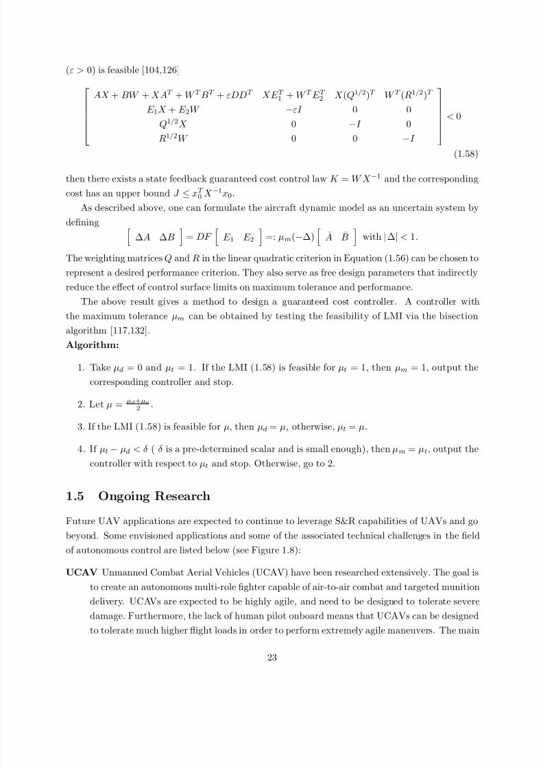
(ε > 0) is feasible [104,126]

AX + BW + XAT + W T BT + εDDT XE T 1 + W T E T

2 X (Q1/2)T W T (R1/2)T

E 1X + E 2W −εI 0 0

Q1/2X 0 −I 0

R1/2W 0 0 −I

< 0

(1.58)

then there exists a state feedback guaranteed cost control law K = W X −1 and the corresponding

cost has an upper bound J ≤ xT 0 X −1x0.

As described above, one can formulate the aircraft dynamic model as an uncertain system by

defining ∆A ∆B

= DF

E 1 E 2

=: µm(−∆)

A B

with |∆| < 1.

The weighting matrices Q and R in the linear quadratic criterion in Equation (1.56) can be chosen to

represent a desired performance criterion. They also serve as free design parameters that indirectly

reduce the effect of control surface limits on maximum tolerance and performance.

The above result gives a method to design a guaranteed cost controller. A controller with

the maximum tolerance µm can be obtained by testing the feasibility of LMI via the bisection

algorithm [117,132].

Algorithm:

1. Take µd = 0 and µt = 1. If the LMI (1.58) is feasible for µt = 1, then µm = 1, output the

corresponding controller and stop.

2. Let µ = µd+µu2 .

3. If the LMI (1.58) is feasible for µ, then µd = µ, otherwise, µt = µ.

4. If µt − µd < δ ( δ is a pre-determined scalar and is small enough), then µm = µt, output the

controller with respect to µt and stop. Otherwise, go to 2.

1.5 Ongoing Research

Future UAV applications are expected to continue to leverage S&R capabilities of UAVs and go

beyond. Some envisioned applications and some of the associated technical challenges in the fieldof autonomous control are listed below (see Figure 1.8):

UCAV Unmanned Combat Aerial Vehicles (UCAV) have been researched extensively. The goal is

to create an autonomous multi-role fighter capable of air-to-air combat and targeted munition

delivery. UCAVs are expected to be highly agile, and need to be designed to tolerate severe

damage. Furthermore, the lack of human pilot onboard means that UCAVs can be designed

to tolerate much higher flight loads in order to perform extremely agile maneuvers. The main

23



technical challenge here is to create autonomous controllers capable of reliably operating in

nonlinear flight regimes for extended durations.

Transport UAVs These UAVs are expected to autonomously deliver valuable and fragile payload

to forward operating units. The technical challenge here is to enable reliable automated

waypoint navigation in presence of external disturbances and changed mass properties, andreliable vertical takeoff and landing capabilities in harsh terrains with significant uncertainties.

HALE High Altitude Long Endurance (HALE) aircraft are being designed to support persistent

S&R missions at stratospheric altitude. The main differentiating factor here is the use of

extended wing span equipped with solar panels for in-situ power generation. The technical

challenges here are brought about by unmodeled flexible body modes.

Optionally Manned Aircraft Optionally manned aircraft are envisioned to support both piloted

and autonomous modes. The idea is to extend the utility of existing successful aircraft by

enabling autonomous operation in absence of an onboard human pilot. The main technicalchallenge here is to ensure reliability and robustness to uncertainties, considering specifically

that these aircraft may share air-space with manned aircraft.

Micro/Nano UAVs UAVs with wingspan less than 30 cm are often referred to as Micro/Nano

UAVs. These UAVs are characterized by high wing (or rotor blade) loading and are being

designed for example to operate in the vicinity of human first-responders. Some of these

aircraft are expected to operate in dynamic or hostile indoor environments, and are therefore

required to be agile and low cost. Large scale collaborative swarms of low-cost micro UAVs

have also been envisioned as flexible replacements to a single larger UAV. The key technical

challenges here are creating low-cost, low-weight controllers capable of guaranteeing safe andagile operation in the vicinity of humans, and development of decentralized techniques for

guidance and control.

In order to realize these visions, there is a need to develop robust and adaptive controllers that

are able to guarantee excellent performance as the UAV performs agile maneuvers in nonlinear flight

regime in presence of uncertainties. Furthermore, there is a significant thrust towards collaborative

operation of manned and unmanned assets and towards UAVs sharing airspace with their manned

counterparts. The predictable and adaptable behavior of UAVs as a part of such co-dependent

networks is evermore important.

1.5.1 Integrated Guidance and Control under Uncertainty

Guidance and Control algorithms for autonomous systems are safety/mission critical. They need

to ensure safe and efficient operation in presence of uncertainties such as unmodeled dynamics,

damage, sensor failure, and unknown environmental effects. Traditionally control and guidance

methods have often evolved separately. The ignored interconnections may lead to catastrophic

24



Figure 1.8: Envisioned UAV applications and some related research thrusts

failure if commanded trajectories end up exciting unmodeled dynamics such as unmodelled flexible

dynamics (modes). Therefore, there is a need to establish a feedback between the guidance and

command loops to ensure that the UAV is commanded a feasible trajectories. This is also impor-

tant in order to avoid actuator saturation, and particularly important if the UAV capabilities have

been degraded due to damage [22]. Isolated works exist in the literature where authors have pro-

posed a scheme to modify reference trajectories to accommodate saturation or to improve tracking

performance (e.g. [51,68]), however, the results are problem specific and more general frameworks

are required.

There has been significant recent research on UAV task allocation and planning algorithms.

The algorithms developed here provide waypoints and reference commands to the guidance system

in order to satisfy higher level mission goals. There may be value in accounting specifically for the

UAV’s dynamic capabilities and health to improve planning performance.

1.5.2 Output Feedback Control in Presence of non-Gaussian noise and Estima-

tion Errors

LQG theory provides a solution to designing optimal controllers for linear systems with Gaussian

white measurement noise. However, such a generalized theory does not exist for nonlinear control.

Furthermore, the choice of sensors on miniature UAVs in particular, is often restricted to low-

cost, low-weight options. Several of the standard sensors employed on miniature aircraft such as

25



sonar altimeters, scanning lasers, and cameras do not have Gaussian noise properties. Therefore,

even with an integrated navigation solution that fuses data from multiple sensors, the resulting

state estimates may contain significant estimation error. One of the key future thrusts required

therefore is a theory of output feedback control for nonlinear control implementations in presence

of non-Gaussian noise.

1.5.3 Metrics on Stability and Performance of UAV controllers

A strong theory exists for computing performance and stability metrics for linear time invariant

control laws. Examples of well accepted metrics include gain and phase margin which quantify the

ability of the controller to maintain stability in presence of unforeseen control effectiveness changes,

time delays, and disturbances. However, these metrics do not easily generalize to nonlinear systems.

On the other hand, several different groups have established that nonlinear control techniques in

general can greatly improve command tracking performance over linear techniques. However, the

inability to quantify stability and robustness of nonlinear controllers may pose a significant hurdle

in wide acceptance of nonlinear techniques. The problem is further complicated as controllers are

implemented on digital computers, while they are often designed using a continuous framework.

Any further work in this area should avail the rich literature on the theory of sampled data systems.

1.5.4 Agile and Fault-Tolerant Control

Agile flight refers to flight conditions which cannot be easily represented by linear models linearized

around equilibrium flight conditions. Agile flight is often characterized by rapid transitions between

flight domains (e.g. hover flight domain and forward flight domain for rotorcraft UAVs), high

wing (blade) loading, actuator saturation, and nonlinear flight regimes. The lack of a human pilotonboard means that the allowable g-force is not a limiting factor on the aggressive maneuvers a UAV

platforms can potentially perform. Significant progress has been made in creating UAV autopilots

that perform highly aggressive maneuvers. Authors in [3,24,34,49] have established control methods

that can be used to perform specific agile maneuvers under test conditions. Future work in this

area could lead to responsive agile flight maneuvers to meet higher level mission requirements and

quantifiable metrics of performance and stability during agile flight.

For some agile flight regimes, accurate modeling of the vehicle dynamics might be very diffi-

cult, requiring that models and/or control strategies be identified in real-time, in essence pushing

the capabilities discussed in [23,47,87,89] to be on-line and for non-linear models. In this case,

model identification (or learning) combined with on-line optimization (e.g., model predictive con-

trol) [30,31,125] might provide an important direction to consider. The key challenge here is to

simultaneously guarantee stability and performance while guaranteeing on-line learning of reason-

able model approximations.

Fault Tolerant Control (FTC) research for UAVs is focused on guaranteeing recoverable flight in

presence of structural and actuator failures. Several directions exist in fault tolerant flight control,

excellent reviews can be found in [119,128]. Authors in [21,52] have established through flight tests

26



the effectiveness of fault tolerant controllers in maintaining flight in presence of severe structural

damage including loss of significant portions of the wing. Detection and diagnosis of structural

faults is also being studied, along with detection of sensor anomalies.

27



Bibliography

[1] Robust Flight Control: A Design Challenge . Lecture Notes in Control and Information Sci-

ences 224. Springer-Verlag, 1997.

[2] Pieter Abbeel, Adam Coates, and Andrew Y. Ng. Autonomous helicopter aerobatics through

apprenticeship learning. The International Journal of Robotics Research , 29(13):1608–1639,

2010.

[3] Pieter Abbeel, Adam Coates, Morgan Quigley, and Andrew Y. Ng. An application of rein-

forcement learning to aerobatic helicopter flight. In Advances in Neural Information Process-

ing Systems (NIPS), page 2007. MIT Press, 2007.

[4] Veronica Adetola, Darryl DeHaan, and Martin Guay. Adaptive model predictive control for

constrained nonlinear systems. Systems and Control Letters , 58(5):320 – 326, 2009.

[5] AIAA. Control of Commercial Aircraft with Vertical Tail Loss . AIAA 4th Aviation Technol-

ogy, Integration, and Operation (ATIO) Forum, 2004. AIAA-2004-6293.

[6] Karl Johan Astrom and Bjorn Wittenmark. Adaptive Control . Addison-Weseley, 2 edition,

1995.

[7] G. Balas, J. Bokor, and Z. Szabo. Invariant subspaces for lpv systems and their applications.

Automatic Control, IEEE Transactions on , 48(11):2065 – 2069, nov. 2003.

[8] A. Bemporad. Reducing conservativeness in predictive control of constrained systems with

disturbances. In Decision and Control, 1998. Proceedings of the 37th IEEE Conference on ,

volume 2, pages 1384 –1389 vol.2, dec 1998.

[9] J. D. Boskovic, R. Prasanth, and R. K. Mehra. Retrofit fault-tolerant flight control design

under control effector damage. AIAA Journal of Guidance, Control and Dynamics , 30(3):703–

712, 2007.

[10] S. Boyd, E. G. Laurent, E. Feron, and V. Balakrishnan. Linear Matrix Inequalities in Systems

and Control . studies in applied mathematics. SIAM, Philadelphia, 1994.

[11] Stephan Boyd and Sankar Sastry. Necessary and sufficient conditions for parameter conver-

gence in adaptive control. Automatica , 22(6):629–639, 1986.

28



[12] Michael S. Branicky. Multiple lyapunov functions and other analysis tools for switched and

hybrid systems. IEEE Transactions on Automatic Control , 43(4):475–482, April 1998.

[13] Anthony Calise and Tansel Yucelen. Adaptive loop transfer recovery. Journal of Guidance

Control and Dynamics , 2012. accepted.

[14] Anthony J. Calise and Rolf T. Rysdyk. Nonlinear adaptive flight control using neural net-

works. IEEE Control Systems Magzine , 18(6):14–25, December 1998.

[15] E. F. Camacho and C. Bordons. Model Predictive Control . Springer, London, 1999.

[16] Chengyu Cao and N. Hovakimyan. Design and analysis of a novel adaptive control architecture

with guaranteed transient performance. Automatic Control, IEEE Transactions on , 53(2):586

–591, march 2008.

[17] L. Chisci, P. Falugi, and G. Zappa. Predictive control for constrained systems with polytopic

uncertainty. In American Control Conference, 2001. Proceedings of the 2001, volume 4, pages3073 –3078 vol.4, 2001.

[18] Girish Chowdhary and Eric N. Johnson. Concurrent learning for convergence in adaptive

control without persistency of excitation. In 49th IEEE Conference on Decision and Control ,

2010.

[19] Girish Chowdhary and Eric N. Johnson. Theory and flight test validation of a concurrent

learning adaptive controller. Journal of Guidance Control and Dynamics , 34(2):592–607,

March 2011.

[20] Girish Chowdhary, Eric N. Johnson, Rajeev Chandramohan, M. Scott Kimbrell, AnthonyCalise, and Hur Jeong. Autonomous guidance and control of an airplane under severe damage.

In AIAA Infotech@Aerospace , 2011. AIAA-2011-1428.

[21] Girish Chowdhary, Eric N. Johnson, Rajeev Chandramohan, Scott M. Kimbrell, and Anthony

Calise. Autonomous guidance and control of airplanes under actuator failures and severe

structural damage. Journal of Guidance Control and Dynamics , 2012. in-press.

[22] Girish Chowdhary, Eric N. Johnson, Scott M. Kimbrell, Rajeev Chandramohan, and An-

thony J. Calise. Flight test results of adaptive controllers in the presence of significant

aircraft faults. In AIAA Guidance Navigation and Control Conference , Toronto, Canada,

2010. Invited .

[23] Girish Chowdhary and Sven Lorenz. Non-linear model identification for a miniature rotor-

craft, preliminary results. In American Helciopter Society 61st Annual Forum , 05.

[24] Mark Cutler and Jonathan P. How. Actuator constrained trajectory generation and control for

variable-pitch quadrotors. In AIAA Guidance, Navigation, and Control Conference (GNC),

Minneapolis, Minnesota, August 2012 (submitted).

29



[25] Francesco A. Cuzzola, Jose C. Geromel, and Manfred Morari. An improved approach for

constrained robust model predictive control. Automatica , 38(7):1183 – 1189, 2002.

[26] H. Demircioglu and E. Karasu. Generalized predictive control. a practical application and

comparison of discrete- and continuous-time versions. Control Systems Magazine, IEEE ,

20(5):36 –47, October 2000.

[27] W. Dunbar. Distributed Receding Horizon Control of Dynamically Coupled Nonlinear Sys-

tems. IEEE Transactions on Robotics , 52:1249–1263, 2007.

[28] W. B. Dunbar and R. Murray. Model Predictive Control of Coordinated Multi-vehicle For-

mations. In IEEE Conference on Decision and Control (CDC), pages 4631–4636, 2002.

[29] W.B. Dunbar and R.M. Murray. Receding horizon control of multi-vehicle formation: A

distributed implementation. In IEEE Conference on Decision and Control (CDC), 2004.

[30] D. Ernst, M. Glavic, F. Capitanescu, and L. Wehenkel. Model predictive control and re-inforcement learning as two complementary frameworks. In Proceedings of the 13th IFAC

Workshop on Control Applications of Optimisation , 2006.

[31] W. Favoreel, B. De Moor, P. Van Overschee, and M. Gevers. Model-free subspace-based

lqg-design. In American Control Conference, 1999. Proceedings of the 1999 , volume 5, pages

3372 –3376 vol.5, 1999.

[32] Hiroaki Fukushima, Tae-Hyoung Kim, and Toshiharu Sugie. Adaptive model predictive con-

trol for a class of constrained linear systems based on the comparison model. Automatica ,

43(2):301 – 308, 2007.

[33] P. Gahinet, A. Nemirovskii, A.J. Laub, and M. Chilali. The lmi control toolbox. In IEEE

Conference on Decision and Control (CDC), volume 3, pages 2038–2041. IEEE, 1994.

[34] V. Gavrilets, B. Mettler, and E. Feron. Human-inspired control logic for automated ma-

neuvering of miniature helicopter. AIAA Journal of Guidance, Control, and Dynamics ,

27(5):752–759, 2004.

[35] Jeremiah Gertler. U.s. unmanned aerial systems. Technical report, Congressional Research

Service, January 2012. Prepared for Members and Committees of Congress.

[36] Wassim M. Haddad and VijaySekhar Chellaboina. Nonlinear Dynamical Systems and Control:

A Lyapunov-Based Approach . Princeton University Press, Princeton, 2008.

[37] C. Hajiyev and F. Caliskan. Fault Diagnosis and Reconfiguration in Flight Control Systems .

Kluwer Academic Publicshers, 2003.

[38] R. Haooouzi and M. Verhaegen. Fault-tolerant subspace predictive control applied to a boeing

747 model. Journal of Guidance, Control and Dynamics , 31(4), July-August 2008.

30



[39] John Hauser and Rick Hindman. Aggressive flight maneuvers. In Proccedings of the 36th

Conference on Decision and Control , San Diego, CA, December 1997. IEEE.

[40] Xu He and Jun Zhao. Parameter-dependent h8 filter design for lpv systems and an autopilot

application. Applied Mathematics and Computation , 218(9):5508 – 5517, 2012.

[41] Y. Hitachi. Damage-tolerant control system design for propulsion-controlled aircraft. Master’s

thesis, University of Toronto, 2009.

[42] Naira Hovakimyan. Robust Adaptive Control . Unpublished, 2008.

[43] Moshe Idan, Matthew D. Johnson, and Anthony J. Calise. A hierarchical approach to adap-

tive control for improved flight safety. AIAA Journal of Guidance Control and Dynamics ,

25(6):1012–1020, nov-dec 2002.

[44] Petros A. Ioannou and Jung Sun. Robust Adaptive Control . Prentice-Hall, Upper Saddle

River, 1996.

[45] R. Isermann. Fault-Diagnosis Systems: An Introduction from Detection to Fault Tolerance .

Springer-Verlag, 2006.

[46] A. Isidori. Nonlinear Control Systems . Springer-Verlag, New York, third edition, 1995.

[47] Ravindra V. Jategaonkar. Flight Vehicle System Identification A Time Domain Approach ,

volume 216 of Progress in Astronautics and Aeronautics . American Institute of Aeronautics

and Astronautics, Reston, 2006.

[48] E. Johnson, M. Turbe, A. Wu, and S. Kannan. Flight results of autonomous fixed-wing

uav transitions to and from stationary hover. In Proceedings of the AIAA GNC Conference ,

August 2006.

[49] Eric Johnson and Suresh Kannan. Adaptive trajectory control for autonomous helicopters.

Journal of Guidance Control and Dynamics , 28(3):524–538, May 2005.

[50] Eric N. Johnson. Limited Authority Adaptive Flight Control . PhD thesis, Georgia Institute

of Technology, Atlanta Ga, 2000.

[51] Eric N. Johnson and Anthony J. Calise. Limited authority adaptive flight control for reusable

launch vehicles. AIAA Journal on Guidance, Control, and Dynamics , 26(6):906–913, Nov-Dec

2003.

[52] Damien B Jourdan, Michael D Piedmonte, Vlad Gavrilets, and David W Vos. Enhancing

UAV Survivability Through Damage Tolerant Control , pages 1–26. Number August. AIAA,

2010. AIAA-2010-7548.

[53] Suresh Kannan. Adaptive Control of Systems in Cascade with Saturation . PhD thesis, Georgia

Institute of Technology, Atlanta Ga, 2005.

31



[54] Srinivas Karra, Rajesh Shaw, Sachin C. Patwardhan, and Santosh Noronha. Adaptive model

predictive control of multivariable time-varying systems. Industrial and Engineering Chem-

istry Research , 47(8):2708–2720, 2008.

[55] E. C. Kerrigan. Robust Constraint Satisfaction Invariant Sets and Predictive Control . PhD

thesis, University of Cambridge, Department of Engineering, November 2000.

[56] E.C. Kerrigan and J.M. Maciejowski. Robust feasibility in model predictive control: neces-

sary and sufficient conditions. In Decision and Control, 2001. Proceedings of the 40th IEEE

Conference on , volume 1, pages 728 –733 vol.1, 2001.

[57] E.C. Kerrigan and D.Q. Mayne. Optimal control of constrained, piecewise affine systems

with bounded disturbances. In Decision and Control, 2002, Proceedings of the 41st IEEE

Conference on , volume 2, pages 1552 – 1557 vol.2, dec. 2002.

[58] H. K. Khalil. Nonlinear Systems . Macmillan, New York, 2002.

[59] Nakawan Kim. Improved Methods in Neural Network Based Adaptive Output Feedback Con-

trol, with Applications to Flight Control . PhD thesis, Georgia Institute of Technology, Atlanta

Ga, 2003.

[60] H. A. Kingravi, G. Chowdhary, P. A. Vela, and E. N. Johnson. Reproducing kernel hilbert

space approach for the online update of radial bases in neuro-adaptive control. Neural Net-

works and Learning Systems, IEEE Transactions on , 23(7):1130 –1141, july 2012.

[61] P.V. Kokotovic. The joy of feedback: nonlinear and adaptive. IEEE Control Systems Maga-

zine , 12(3):7–17, 1992.

[62] Shauying R. Kou, David L. Elliott, and Tzyh Jong Tarn. Observability of nonlinear systems.

Information and Control , 22(1):89 – 99, 1973.

[63] Emre Koyuncu, N. Ure, and Gokhan Inalhan. Integration of path/maneuver planning in

complex environments for agile maneuvering ucavs. Journal of Intelligent & Robotic Systems ,

57:143–170, 2010. 10.1007/s10846-009-9367-1.

[64] Miroslav Krstic, Ioannis Kanellakopoulos, and Petar Kokotovic. Nonlinear and Adaptive

Control Design . John Wiley and Sons, 1995.

[65] Ali Kutay, Girish V. Chowdhary, A. Calise, and Eric N. Johnson. A comparision of two novel

direct adaptive control methods under actuator failure accommodation. In Proceedings of the

AIAA GNC Conference, held at Honolulu, HI , 2008.

[66] Eugene Lavertsky and Kevin Wise. Flight control of manned/unmanned military aircraft. In

Proceedings of American Control Conference , 2005.

32



[67] E. Lavretsky. Combined/composite model reference adaptive control. Automatic Control,

IEEE Transactions on , 54(11):2692 –2697, nov. 2009.

[68] Eugene Lavretsky. Reference dynamics modification in adaptive controllers for improved tran-

sient performance. In Guidance Navigation and Control Conference , Portland, OR, August

2011. AIAA. AIAA-2011-6200.

[69] Chirl Hwa Lee, Myoung Ho Shin, and Myung Jin Chung. A design of gain-scheduled control

for a linear parameter varying system: an application to flight control. Control Engineering

Practice , 9(1):11 – 21, 2001.

[70] J. H. Lee. Nonlinear Model Predictive Control , volume 26 of Progress in Systems and Control

Theory , chapter Modeling and identification for nonlinear model predictive control: require-

ments, current status and future research needs, pages 269–294. Birkhauser, Basel-Boston-

Berlin, 2000.

[71] Kwan Ho Lee, Joon Hwa Lee, and Wook Hyun Kwon. A stabilizing low-order output feedback

receding horizon control for linear discrete time-invariant systems. In American Control

Conference, 2002. Proceedings of the 2002 , volume 3, pages 2412 – 2417 vol.3, 2002.

[72] Y. I. Lee and B. Kouvaritakis. Constrained receding horizon predictive control for systems

with disturbances. International journal of control , 72(11):1027–1032, 1999.

[73] Y.I. Lee and B. Kouvaritakis. A linear programming approach to constrained robust predictive

control. Automatic Control, IEEE Transactions on , 45(9):1765 –1770, sep 2000.

[74] A. Levant, A. Pridor, R. Gitizadeh, I. Yaesh, and J. Z. Ben-Asher. Aircraft pitch control viasecond order sliding techniques. Journal of Guidance, Control, and Dynamics , 23:586–594,

2000.

[75] F. L. Lewis. Nonlinear network structures for feedback control. Asian Journal of Control ,

1:205–228, 1999. Special Issue on Neural Networks for Feedback Control.

[76] Xiaobo Li and Hugh H. T. Liu. A passive fault tolerant flight control for maximum allowable

vertical tail damaged aircraft. Journal of Dynamic Systems, Measurement, and Control , to

appear.

[77] D. Liberzon. Switching in Systems and Control . Birkhauser, Boston, MA, 2003.

[78] Daniel Liberzon. Handbook of Networked and Embedded Control Systems , chapter Switched

Systems, pages 559–574. Birkhauser, Boston, 2005.

[79] D. Limon Marruedo, T. Alamo, and E.F. Camacho. Stability analysis of systems with bounded

additive uncertainties based on invariant sets: Stability and feasibility of mpc. In American

Control Conference, 2002. Proceedings of the 2002 , volume 1, pages 364 – 369 vol.1, 2002.

33



[80] T. J. J. Lombaerts, H. O. Huisman, Q. P. Chu, J. A. Mulder, and D. A. Joosten. Nonlinear

reconfiguring flight control based on online physical model identification. In AIAA Guidance,

Navigation and Control Conference and Exhibit , August 18-21 2008.

[81] J. Lunze and T. Steffen. Control reconfiguration after actuator failures using disturbance

decoupling methods. IEEE Transactions on Automatic Control , 51(10):1590–1601, October2006.

[82] J. M. Maciejowski. Predictive control with constraints . Prentice hall publications, 2002.

[83] V. Manikonda, P.O. Arambel, M. Gopinathan, R.K. Mehra, and F.Y. Hadaegh. A model

predictive control-based approach for spacecraft formation keeping and attitude control. In

American Control Conference, 1999. Proceedings of the 1999 , volume 6, pages 4258 –4262

vol.6, 1999.

[84] I. Masubuchi, J. Kato, M. Saeki, and A. Ohara. Gain-scheduled controller design based on

descriptor representation of lpv systems: application to flight vehicle control. In Decision and

Control, 2004. CDC. 43rd IEEE Conference on , volume 1, pages 815 –820 Vol.1, dec. 2004.

[85] D. Q. Mayne. Nonlinear Model Predictive Control , volume 26 of Progress in Systems and

Control Theory , chapter Nonlinear Model Predictive Control: Challenges and Opportunities,

pages 23–44. Birkhauser, Basel-Boston-Berlin, 2000.

[86] D. Q. Mayne, J. B. Rawlings, C. V. Rao, and P. O. M. Scokaert. Constrained model predictive

control: Stability and optimality. Automatica , 36:789–814, 2000.

[87] B. Mettler. Identification modeling and characteristics of miniature rotorcraft . Springer, 2003.

[88] H. Michalska and D.Q. Mayne. Moving horizon observers and observer-based control. Auto-

matic Control, IEEE Transactions on , 40(6):995 –1006, jun 1995.

[89] E. A. Morelli. Real time parameter estimation in the frequency domain. Journal of Guidance

Control and Dynamics , 23(5):812–818, 2000.

[90] Flavio Nardi. Neural Network based Adaptive Algorithms for Nonlinear Control . PhD thesis,

Georgia Institute of Technology, School of Aerospace Engineering, Atlanta, GA 30332, nov

2000.

[91] K. Narendra and A. Annaswamy. A new adaptive law for robust adaptation without persistent

excitation. IEEE Transactions on Automatic Control , 32(2):134–145, February 1987.

[92] Kumpati S. Narendra and Anuradha M. Annaswamy. Stable Adaptive Systems . Prentice-Hall,

1989.

34



[93] N. Nguyen, K. Krichnamumar, and J. Kaneshige. Dynamics and adaptive control for stability

recovery of damaged asymmetric aircraft,. In AIAA Guidance, Navigation, and Control

Conference and Exhibits , August 21-24 2006. AIAA-2006-6049.

[94] N. Nguyen, K. Krishnakumar, and J. Kaneshige. Flight dynamics and hybrid adaptive control

of damaged aircraft. AIAA Journal of Guidance, Control, and Dynamics , 31(3):751–764,2008.

[95] Nhan Nguyen. Asymptotic linearity of optimal control modification adaptive law with ana-

lytical stability margins. In Infotech@AIAA conference , Atlanta, GA, 2010.

[96] Nhan Nguyen, Kalamanje Krishnakumar, John Kaneshige, and Pascal Nespeca. Dynamics

and adaptive control for stability recovery of damaged asymmetric aircraft. In AIAA Guidance

Navigation and Control Conference , Keystone, CO, 2006.

[97] G. D. Nicolao, L. Magi, and R. Scattolini. Nonlinear Model Predictive Control , volume 26

of Progress in Systems and Control Theory , chapter Stability and Robustness of Nonlinear

Receding Horizon Control, pages 3–22. Birkhauser, Basel-Boston-Berlin, 2000.

[98] H. Nijmeijer and A.J. van der Schaft. Nonlinear Dynamical Control Systems . Springer-Verlag,

New York, 1990.

[99] Office of the Secretary of Defense. Unmanned aircraft systems roadmap 2005-2030. Technical

report, Department of Defense, August 2005.

[100] Office of the Secretary of Defense. Unmanned aircraft systems roadmap. Technical report,

OSD, 2007.

[101] J. Park and I.W. Sandberg. Universal approximation using radial-basis-function networks.

Neural Computatations , 3:246–257, 1991.

[102] V. Patel, C. Cao, N. Hovakimyan, K. Wise, and E. Lavretsky. Adaptive controller for tailless

unstable aircraft in the presence of unknown actuator failures. International Journal of

Control , 82(4):705–720, 2009.

[103] R. J. Patton and J. Chen. Fault-tolerant control systems: The 1997 situation. In IFAC

Symposium on Fault Detection Supervision and Safety for Technical Processes , pages 1033–

1054, UK, 1997. Kingston Upon Hull.

[104] I. R. Petersen, V. A. Ugrinovskii, and A. V. Savkin. Robust Control Design using H ∞

Methods . Communications and Control Engineering Series. Springer-Verlag, 2000.

[105] Findeisen R., L. Imsland, F. Allgower, and B. A. Foss. Output feedback stabilization of

constrained systems with nonlinear predictive control. International journal of robust and

nonlinear control , 13:211–227, 2003.

35



[106] Ioannis A. Raptis and Kimon P. Valavanis. Linear and Nonlineaer Control of Small-Scale

Unmanned Helicopters , volume 45 of International Series on Intelligent Systems, Control,

and Automation: Science and Engineering . Springer, Heidelberg, 2011.

[107] J.B. Rawlings. Tutorial overview of model predictive control. Control Systems Magazine,

IEEE , 20(3):38 –52, June 2000.

[108] A. Richards and J. P. How. Decentralized model predictive control of cooperating UAVs.

In IEEE Conference on Decision and Control (CDC), pages 4286–4291, Paradise Island,

Bahamas, December 2004.

[109] A. Richards and J. P. How. Robust decentralized model predictive control. International

Journal of Control , 80(9):1517–1531, Sept. 2007.

[110] Arthur G. Richards. Robust Constrained Model Predictive Control . PhD thesis, Massachusetts

Institute of Technology, Department of Aeronautics and Astronautics, Cambridge MA, Febru-

ary 2005.

[111] L. Rodrigues and J. P. How. Observer-based control of piecewise-affine systems. International

Journal of Control , 76(5):459–477, 2003.

[112] R.M. Sanner and J.-J.E. Slotine. Gaussian networks for direct adaptive control. Neural

Networks, IEEE Transactions on , 3(6):837 –863, nov 1992.

[113] M. A. Santillo and D. S. Bernstein. Adaptive control based on retrospective cost optimization.

AIAA Journal of Guidance Control and Dynamics , 33(2), March-April 2010.

[114] G.H. Shah. Aerodynamic effects and modeling of damage to transport aircraft. Technical

report, NASA Langley Research Center, Hampton, VA, 2008.

[115] Jeff S. Shamma and Michael Athans. Guaranteed properties of gain scheduled control for

linear parameter-varying plants. Automatica , 27(3):559 – 564, 1991.

[116] I. A. Shkolnikov and Y. B. Shtessel. Aircraft nonminimal phase control in dynamic sliding

manifolds. Journal of Guidance, Control, and Dynamics , 24:566–573, 2001.

[117] Sigurd Skogestad and Ian Postlethwaite. Multivariable Feedback Control - Analysis and De-

sign . John Wiley and Sons Ltd, 2005.

[118] J. E. Slotine and W. Li. Applied Nonlinear Control . Prentice-Hall, Englewood Cliffs, NJ,

1991.

[119] M. Steinberg. Historical overview of research in reconfigurable flight control. Proceedings of the

Institution of Mechanical Engineers, Part G: Journal of Aerospace Engineering , 219(4):263–

275, 2005.

36



[120] N. Sundararajan, P. Saratchandran, and L. Yan. Fully Tuned Radial Basis Function Neural

Networks for Flight Control . Springer, 2002.

[121] Gordon J. Sutton and Robert R. Bitmead. Nonlinear Model Predictive Control , volume 26 of

Progress in Systems and Control Theory , chapter Performance and Computational Implemen-

tation of Nonlinear Model Predictive Control on a Submarine, pages 461–472. Birkhauser,Basel-Boston-Berlin, 2000.

[122] Gang Tao. Adaptive Control Design and Analysis . Wiley, 2003.

[123] U. S. Army UAS Center of Excellence. “Eyes of the Army” U. S. Army Unmanned Aircraft

Systems Roadmap 2010-2035, 2010.

[124] Kostyantyn Y. Volyanskyy, Wassim M. Haddad, and Anthony J. Calise. A new neuroad-

aptive control architecture for nonlinear uncertain dynamical systems: Beyond σ and e-

modifications. IEEE Transactions on Neural Networks , 20(11):1707–1723, Nov 2009.

[125] B.R. Woodley, J.P. How, and R.L. Kosut. Model free subspace based hscr; infin; control. In

American Control Conference, 2001. Proceedings of the 2001, volume 4, pages 2712 –2717

vol.4, 2001.

[126] L. Yu. Robust Control: Linear Matrix Inequality Approach . Tshinghua University Press, in

chinese edition, 2002.

[127] Tansel Yucelen and Anthony Calise. A derivative-free model reference adaptive controller

for the generic transport model. In AIAA Guidance, Control and Navigation Conference ,

Toronto, Canada, August 2010. invited.

[128] Youmin Zhang and Jin Jang. Bibliographical review on reconfigurable fault-tolerant control

systems. Elsevier Annual Reviews in Control , 32(1):229–252, 2008.

[129] Zhi-sheng Zhang, Huai-min Chen, Cheng-fu Wu, and Ma Song-hui. An effective terminal con-

dition ensuring stability of mpc. In Computer Application and System Modeling (ICCASM),

2010 International Conference on , volume 7, pages V7–202 –V7–206, 2010.

[130] A. Zheng and F. Allgower. Towards a practical nonlinear predictive control algorithm with

guaranteed stability for large-scale systems. In American Control Conference, 1998. Proceed-

ings of the 1998 , volume 4, pages 2534 –2538 vol.4, June 1998.

[131] Alex Zheng. Nonlinear Model Predictive Control , volume 26 of Progress in Systems and

Control Theory , chapter Some practical issues and possible solutions for nonlinear model

predictive control, pages 129–144. Birkhauser, Basel-Boston-Berlin, 2000.

[132] K. Zhou, J. C. Doyle, and K. Glover. Robust and Optimal Control . Prentice-Hall, Englewood

uav nonlinear flight controls chapter

Documents