research purpose & scope
TRANSCRIPT

BAYESIAN BELIEF NETWORKS: A CONCEPTUAL APPROACH TO
ASSESSING RISK TO HABITAT
By
Kelli J. Taylor
A report submitted in partial fulfillment of the requirements for the degree
of
MASTER OF SCIENCE
In
Bioregional Planning
Approved:
___________________________ ___________________________ Richard Toth R. Douglas Ramsey Major Professor Major Professor
___________________________ ___________________________ John A. Bissonette Douglas Jackson-Smith Committee Member Committee Member
UTAH STATE UNIVERSITY Logan, Utah
2003

Copyright © Kelli J. Taylor 2003 All Rights Reserved
ABSTRACT
BAYESIAN BELIEF NETWORKS: A CONCEPTUAL FRAMEWORK FOR ASSESSING RISK TO HABITAT
by
Kelli J. Taylor, Master of Science
Utah State University, 2003
Major Professors: R. Douglas Ramsey Richard Toth
Department: Environment and Society
I developed an integrated application of Bayesian belief networks with
Geographic Information Systems to provide a framework for assessing risk relative to
wildlife habitat in the southern Wind River landscape of southwestern Wyoming.
The Bayesian belief network applied in this research is a graphical, probabilistic model
representing cause and effect relationships (Pearl 1988; Jensen 1996). Further
explanation of Bayesian statistics and of Bayesian belief networks is discussed in the
“Methods” section on page 42.
Specifically, I conducted an assessment of risk(s) to mule deer (Artiodactyla
cervidae), sage grouse (Centrocercus urophasianus) and mink (Mustela vison) habitat
from anthropogenic activity based on professional opinion. Local wildlife and habitat
expert opinion was vital in compiling and ranking risks. In an informal interview
process, experts were asked to rank risk as being either ‘high’, ‘medium’, ‘low’ or as
having ‘no’ risk. The rankings were used to develop the Bayesian belief network that
iii

provided probabilities of risk. The probability values were then used to in a Geographic
Information System to create a spatial representation of landscape risk. As a decision-
making tool, the Bayesian network models may provide a tool for adaptive land-use
planning and management strategies.
iv
ACKNOWLEDGEMENTS
I would like to start by acknowledging the support of those who put me on the path that I have enjoyed so much. My parents and grandparents encouraged me in my studies and gave me both the freedom and support that I needed to become the person I am. They trusted in me enough to let me choose my own goals. I hope that I have lived up to their expectations. Many teachers have also influenced me, but I would like to give special thanks to Daniel P. Ames for your encouragement, enthusiam and for the long hours spent outside of your own work to share in the creation of this project.
I have laughed, cried and grown immeasurably from my friendship and discussions with fellow graduate students Wendy Reith and Lisa Langs along with many others. I am grateful for the assistance of Bethany Nielsen and Ahmed Said during the early stages of this work. More recently, I give a special thanks to the folks at Wyoming Game & Fish Dept. for their continued support and flexibility.
Thanks to my friends, Liz Didier, Sarah Rooney, Laura Blonski, Carey Hendrix
and Cindy Yurth who played such important roles along the journey in providing encouragement, love and laughter at those times when it seemed impossible to continue.
I offer my gratitude and appreciation to my committee members, Doug Ramsey and Dick Toth who supported me through out the whole of this work. I offer special thanks to John Bissonette who taught me to love Landscape Ecology and who jumped in with both feet to support me on my path; and, to Douglas Jackson-Smith for reminding me to keep my eyes on the prize. And a special thanks to Mark Brunson, John Malechek, Dale Blahna, Joanna Enta-Wada, Judy Kurtzman, the gang from the old Spatial Ecology lab for keeping me laughing, and to the CNR Business Office.
Financial support was provided by NASA/ARC, Dennis Wright my final year. And, a special thanks goes to Tom Edwards for his generosity, patience, grace and kind words during my time at USU. Thank you for your understanding heart.
Most of all thanks to the divine spirit for the natural beauty of Sandhill cranes,
short-eared owls and the Harriers at Bud Phelps. The peace of all those long walks there on still mornings and quiet evenings with the wonderful Little Black Dog gave me solace and strength making this an endurable journey.
v

CONTENTS
Page
ABSTRACT......................................................................................................... i
ACKNOWLEDGEMENTS.................................................................................iv
LIST OF FIGURES .............................................................................................vi
LIST OF TABLES...............................................................................................vii
INTRODUCTION ...............................................................................................10 Research Purpose and Scope ...................................................................11 Key Definitions........................................................................................16 STUDY SITE DESCRIPTION............................................................................18 LITERATURE REVIEW ....................................................................................25
METHODS ..........................................................................................................37 Data Collection ........................................................................................38
Bayesian Networks ..................................................................................45 Interview Methodology............................................................................47
RESULTS ............................................................................................................54 Risk Maps ................................................................................................64 DISCUSSION......................................................................................................71
REFERENCES ....................................................................................................76
APPENDICES .....................................................................................................84 Appendix A: Maps...................................................................................85 Appendix B: Questionnaire and Interview Results..................................100 Appendix C: BBN Models.......................................................................117 Appendix D: Conditional Probability Tables ..........................................120 Appendix E: Sensitivity Analyses ..........................................................123
vi
LIST OF FIGURES
FIGURE Page
1. Greater Yellowstone Ecosystem.....................................................................18
2. Wyoming and Study Area...............................................................................19
3. Southern Wind River Landscape ....................................................................20
4. A cushion plant example..................................................................................22
5. Mule deer seasonal habitat map.......................................................................41
6. Sage grouse seasonal habitat map....................................................................42
7. Mink habitat map .............................................................................................43
8. Risk map for mink ...........................................................................................65
9. Risk map for mink at Red Canyon Ranch .......................................................66
10. Risk map for sage grouse...............................................................................67
11. Risk map for sage grouse at Red Canyon Ranch...........................................68
12. Risk map for mule deer..................................................................................69
13. Risk map for mule deer at Red Canyon Ranch..............................................70
vii
LIST OF TABLES
TABLES Page
1. GIS Data, buffers and source ...........................................................................39
2. Conditional probability table for mink ............................................................46
3. Conditional probability table for sage grouse..................................................61
viii

LIST OF GRAPHS
GRAPHS Page
1. A graphical representation of a belief network................................................32
2. A Bayesian belief network for mink................................................................51
3. Mule deer probability averages for surface features........................................55
4. Expert variability for mule deer seasonal habitat probabilities .......................57
5. Sage grouse probability averages for surface features.....................................58
6. Mule deer probability estimates for seasonal habitat.......................................59
ix
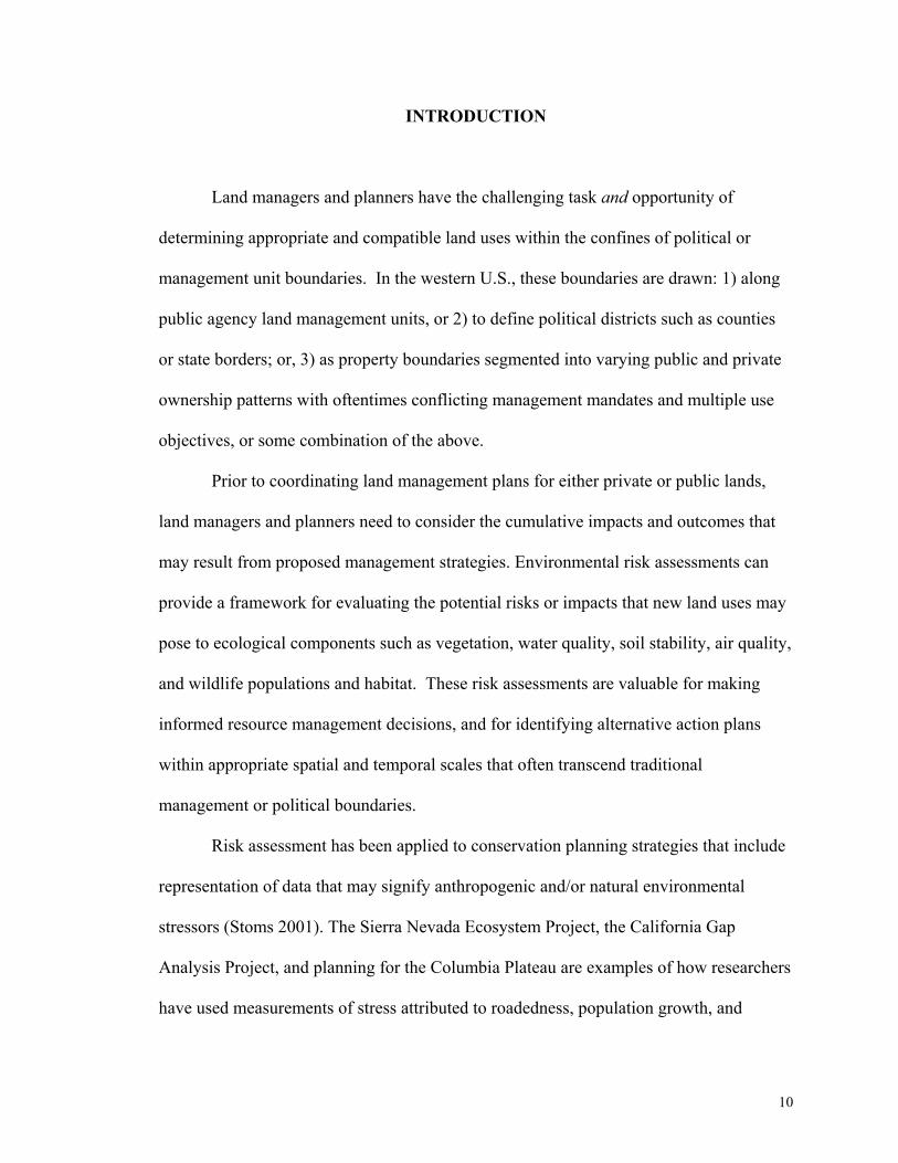
INTRODUCTION
Land managers and planners have the challenging task and opportunity of
determining appropriate and compatible land uses within the confines of political or
management unit boundaries. In the western U.S., these boundaries are drawn: 1) along
public agency land management units, or 2) to define political districts such as counties
or state borders; or, 3) as property boundaries segmented into varying public and private
ownership patterns with oftentimes conflicting management mandates and multiple use
objectives, or some combination of the above.
Prior to coordinating land management plans for either private or public lands,
land managers and planners need to consider the cumulative impacts and outcomes that
may result from proposed management strategies. Environmental risk assessments can
provide a framework for evaluating the potential risks or impacts that new land uses may
pose to ecological components such as vegetation, water quality, soil stability, air quality,
and wildlife populations and habitat. These risk assessments are valuable for making
informed resource management decisions, and for identifying alternative action plans
within appropriate spatial and temporal scales that often transcend traditional
management or political boundaries.
Risk assessment has been applied to conservation planning strategies that include
representation of data that may signify anthropogenic and/or natural environmental
stressors (Stoms 2001). The Sierra Nevada Ecosystem Project, the California Gap
Analysis Project, and planning for the Columbia Plateau are examples of how researchers
have used measurements of stress attributed to roadedness, population growth, and
10
invasive plant species to identify potential “train wrecks” where biodiversity and
stressors converge (Stoms 2001) at a landscape scale.
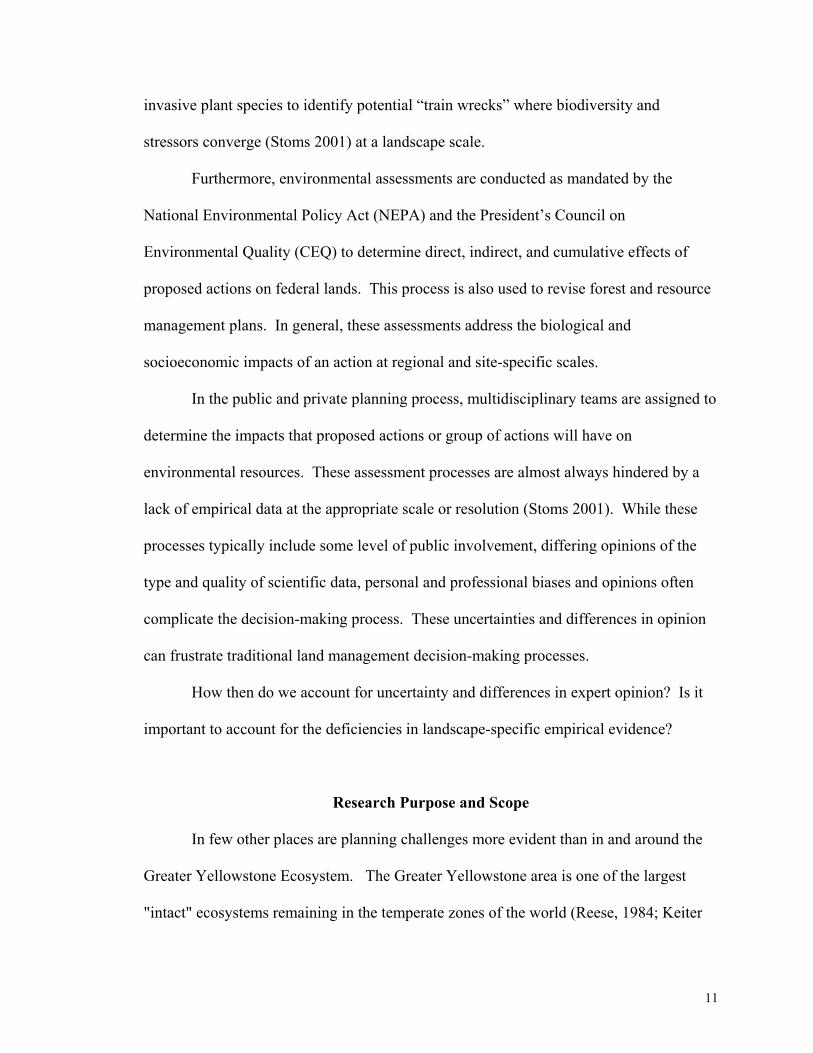
Furthermore, environmental assessments are conducted as mandated by the
National Environmental Policy Act (NEPA) and the President’s Council on
Environmental Quality (CEQ) to determine direct, indirect, and cumulative effects of
proposed actions on federal lands. This process is also used to revise forest and resource
management plans. In general, these assessments address the biological and
socioeconomic impacts of an action at regional and site-specific scales.
In the public and private planning process, multidisciplinary teams are assigned to
determine the impacts that proposed actions or group of actions will have on
environmental resources. These assessment processes are almost always hindered by a
lack of empirical data at the appropriate scale or resolution (Stoms 2001). While these
processes typically include some level of public involvement, differing opinions of the
type and quality of scientific data, personal and professional biases and opinions often
complicate the decision-making process. These uncertainties and differences in opinion
can frustrate traditional land management decision-making processes.
How then do we account for uncertainty and differences in expert opinion? Is it
important to account for the deficiencies in landscape-specific empirical evidence?
Research Purpose and Scope
In few other places are planning challenges more evident than in and around the
Greater Yellowstone Ecosystem. The Greater Yellowstone area is one of the largest
"intact" ecosystems remaining in the temperate zones of the world (Reese, 1984; Keiter
11

and Boyce 1991). According to Knight (1994), the Greater Yellow Ecosystem is one of
the world's foremost natural laboratories in landscape ecology and geology and is a
world-renowned recreational site. Concerns for public land managers and interest groups
include eroding ecological integrity, maintaining the unique plant and animal
communities, wildlife migration corridors, and seasonal ranges critical to the well-being
of wildlife, and the overall fragmentation of the Yellowstone ecosystem (Hansen et al.
online). Managing diverse and sometimes conflicting and competing land uses in the
region are daunting tasks for public and private land managers, area residents, and
advocacy groups. Public and private groups have organized in the last decade to address
the multitude of conflicting uses in the region.
The Southern Wind River Landscape (SWRL) is the southern most extension of
the Greater Yellowstone Ecosystem located in west central Wyoming. Despite its
proximity to the more populated and faster growing Yellowstone region, the nearly three
million acre SWRL remains largely intact. As part of the ecoregional planning process,
the Nature Conservancy recently has completed a preliminary conservation plan for the
SWRL. A goal of the planning process is to develop an integrated ecological
conservation strategy that restores and/or maintains linkages between habitat as well as
buffer key habitat patches, i.e., to identify relatively intact, contiguous patches of
landscape that ensure a measure of biodiversity (TNC 2001).
As part of the planning process, a risk assessment may identify conservation
priorities in the context of large ecological systems and human use of the landscape
(personal communication, TNC 2002). As an example of this planning strategy, a central
12

planning component includes ranking threats and stressors relative to biodiversity and
landscape connectivity.
Risk assessment, as applied to this project, is defined as the probability of a
specific undesired effect resulting from the existence of a hazard and uncertainty about its
expression (Suter 1996). The assessment addresses some present or future impact(s) or an
estimation of the probabilities of outcomes. Estimating relative risk is important to any
assessment process. Selecting a means of quantifying risk represents some challenges.
Some commonly used criteria for ranking risks include determining areas of risk,
estimating the severity and magnitude of effects, understanding the temporal aspects of
impacts, such as reversibility, or quantifying the ecological “value” of the system (Varis
1995).
The ranking process is built upon existing scientific knowledge, databases,
literature, and expert opinion but often ignores uncertainty or professional disagreements
(Morgan and Henrion 1990). Data and information is often extrapolated from dissimilar
research sites and geographic regions. Inferences and decisions are then made that relate
threats, risk, and effects of disturbance events on the landscape of interest. As a result,
assessment conclusions can be misleading. This uncertainty begs the questions: 1) Is a
landscape level, standardized methodology of quantifying threats or risk for a particular
landscape, ecosystem, eco-region, or habitat(s) appropriate; and 2) If not, what alternative
method would be appropriate for quantifying or ranking relative risk?
Some progress has been made in predicting impacts on species and habitat using
urban growth simulations (White et al. 1997, Landis et al. 1998, Duane 1999). However,
definitive empirical research required for completing a landscape level habitat risk
13
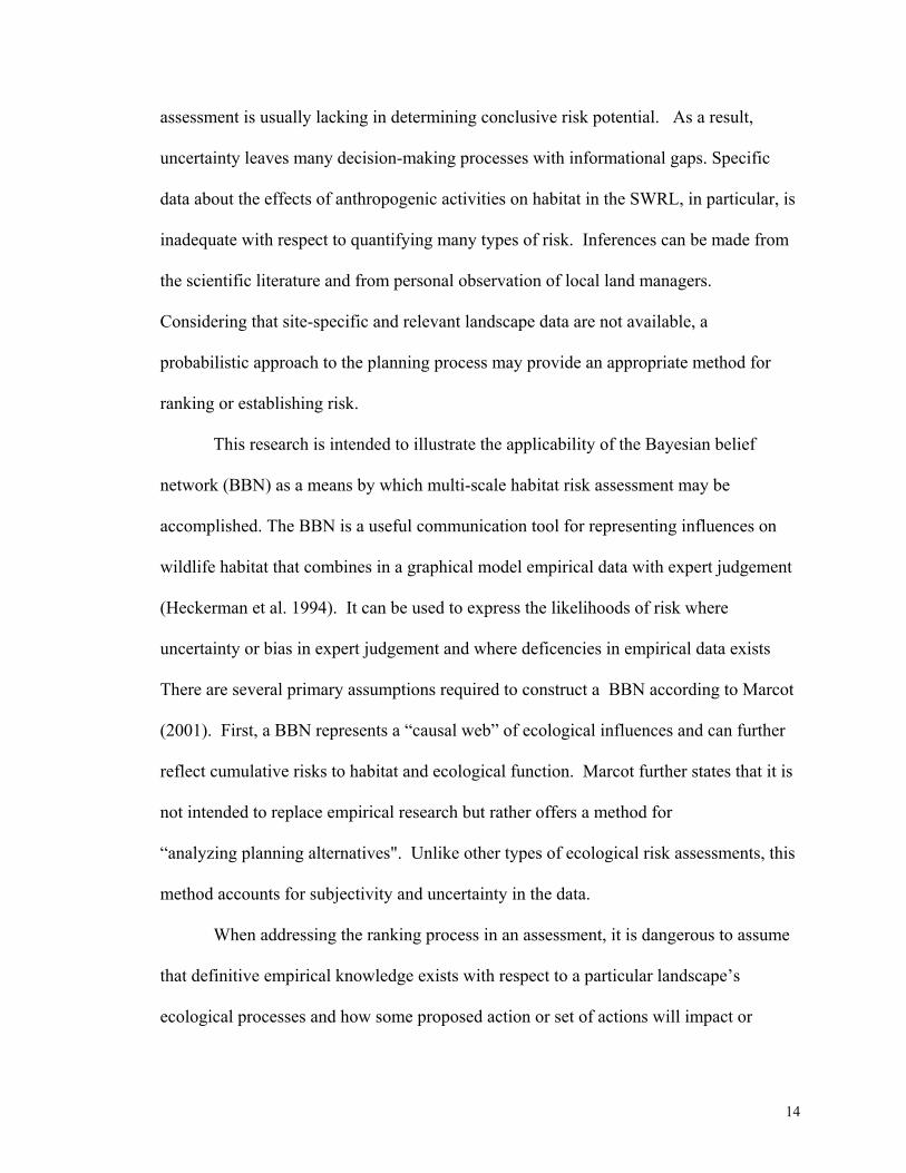
assessment is usually lacking in determining conclusive risk potential. As a result,
uncertainty leaves many decision-making processes with informational gaps. Specific
data about the effects of anthropogenic activities on habitat in the SWRL, in particular, is
inadequate with respect to quantifying many types of risk. Inferences can be made from
the scientific literature and from personal observation of local land managers.
Considering that site-specific and relevant landscape data are not available, a
probabilistic approach to the planning process may provide an appropriate method for
ranking or establishing risk.
This research is intended to illustrate the applicability of the Bayesian belief
network (BBN) as a means by which multi-scale habitat risk assessment may be
accomplished. The BBN is a useful communication tool for representing influences on
wildlife habitat that combines in a graphical model empirical data with expert judgement
(Heckerman et al. 1994). It can be used to express the likelihoods of risk where
uncertainty or bias in expert judgement and where deficencies in empirical data exists
There are several primary assumptions required to construct a BBN according to Marcot
(2001). First, a BBN represents a “causal web” of ecological influences and can further
reflect cumulative risks to habitat and ecological function. Marcot further states that it is
not intended to replace empirical research but rather offers a method for
“analyzing planning alternatives". Unlike other types of ecological risk assessments, this
method accounts for subjectivity and uncertainty in the data.
When addressing the ranking process in an assessment, it is dangerous to assume
that definitive empirical knowledge exists with respect to a particular landscape’s
ecological processes and how some proposed action or set of actions will impact or
14
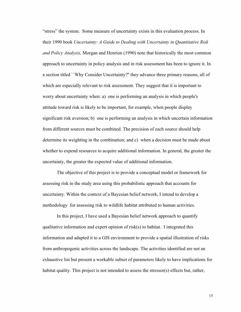
“stress” the system. Some measure of uncertainty exists in this evaluation process. In
their 1990 book Uncertainty: A Guide to Dealing with Uncertainty in Quantitative Risk
and Policy Analysis, Morgan and Henrion (1990) note that historically the most common
approach to uncertainty in policy analysis and in risk assessment has been to ignore it. In
a section titled ``Why Consider Uncertainty?'' they advance three primary reasons, all of
which are especially relevant to risk assessment. They suggest that it is important to
worry about uncertainty when: a) one is performing an analysis in which people's
attitude toward risk is likely to be important, for example, when people display
significant risk aversion; b) one is performing an analysis in which uncertain information
from different sources must be combined. The precision of each source should help
determine its weighting in the combination; and c) when a decision must be made about
whether to expend resources to acquire additional information. In general, the greater the
uncertainty, the greater the expected value of additional information.
The objective of this project is to provide a conceptual model or framework for
assessing risk in the study area using this probabilistic approach that accounts for
uncertainty. Within the context of a Bayesian belief network, I intend to develop a
methodology for assessing risk to wildlife habitat attributed to human activities.
In this project, I have used a Bayesian belief network approach to quantify
qualitative information and expert opinion of risk(s) to habitat. I integrated this
information and adapted it to a GIS environment to provide a spatial illustration of risks
from anthropogenic activities across the landscape. The activities identified are not an
exhaustive list but present a workable subset of parameters likely to have implications for
habitat quality. This project is not intended to assess the stressor(s) effects but, rather,
15
identify and rank probabilities of risk from local and regional habitat stressors to mule
deer, mink and sage grouse habitat. The stressors included in this study involve land
development in or near critical wildlife habitat, oil and natural gas development, and
roads across the landscape.
Three steps provide a framework for assessing risk to habitat from human-related
activities: 1) collection of spatial data; (2) modeling risk probability using a Bayesian
belief network; and (3) integration of GIS data with the risk models to spatially represent
risk across the landscape.
As a central element to the model development, spatial analysis and quantification
of cumulative disturbance(s) were assessed using GIS to illustrate multi-scale disturbance
patterns. Recognition of present risks and potential risks to habitat across the landscape
can inform a methodology for better habitat planning (Marcot 2001). This process may
also provide a decision support tool given the limited scientific data available to land
managers, wildlife managers and the interested public.
Key Definitions
The following terms will be used throughout the project.
Cumulative Risk: The combined risks from aggregate exposures to multiple agents or
stressors (USEPA 2003) Cumulative risk assessment: An analysis, characterization, and possible quantification
of the combined risks to health or the environment from multiple agents or stressors (USEPA 2003).
Disturbances: are events that disrupt ecological systems; they may occur naturally [e.g.,
wildfires, storms, or floods or be induced by human actions, such as clearing for agriculture, clear-cut in forests, building roads, or altering stream channels (ESA Committee on Land Use).
16
Habitat: is based on the WYGAP analysis GIS habitat layers at a coarse scale anda
finer data taken from the Wyoming Department of Game and Fish. A less formal definition of habitat is provided by Begon et al. as the place where a microorganism, plant or animal lives (1996).
Multiple stressor assessments: Exposures can be accumulated over time, pathways,
sources, or routes for a number of agents or stressors. These stressors may cause the same effects (e.g., a number of carcinogenic chemicals or a number of threats to habitat loss), or a variety of effects. A risk assessment for multiple stressors may evaluate the risks of the stressors associated health effects or ecological impacts, one effect or impact at a place (USEPA 2003).
Stressor: is a physical, chemical, biological, or other entity that can cause an adverse
response in a human or other organism or ecosystem. A stressor can be exposure to a chemical, biological, or physical agent (e.g., radon), or it may be the lack of, or destruction of, some necessity such as a habitat. A socioeconomic stressor, for example, might be the lack of needed health care, which could lead to adverse effects (USEPA 2003).
17
STUDY SITE
The Southern Wind River Landscape
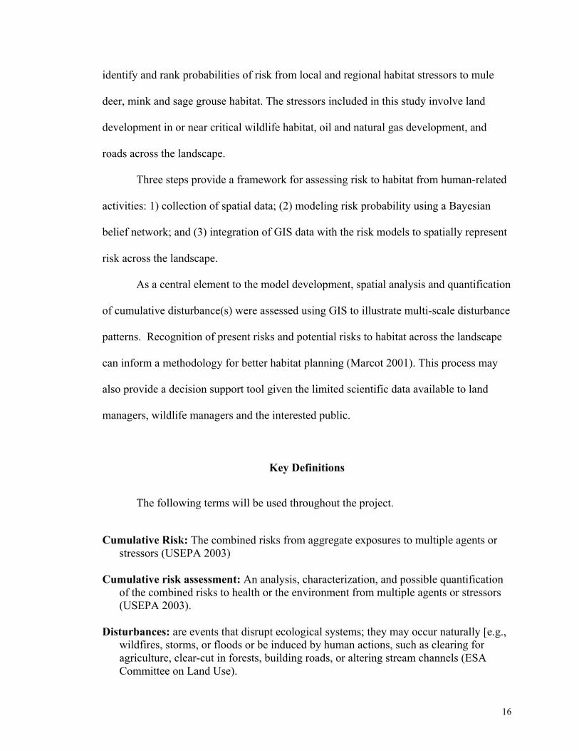
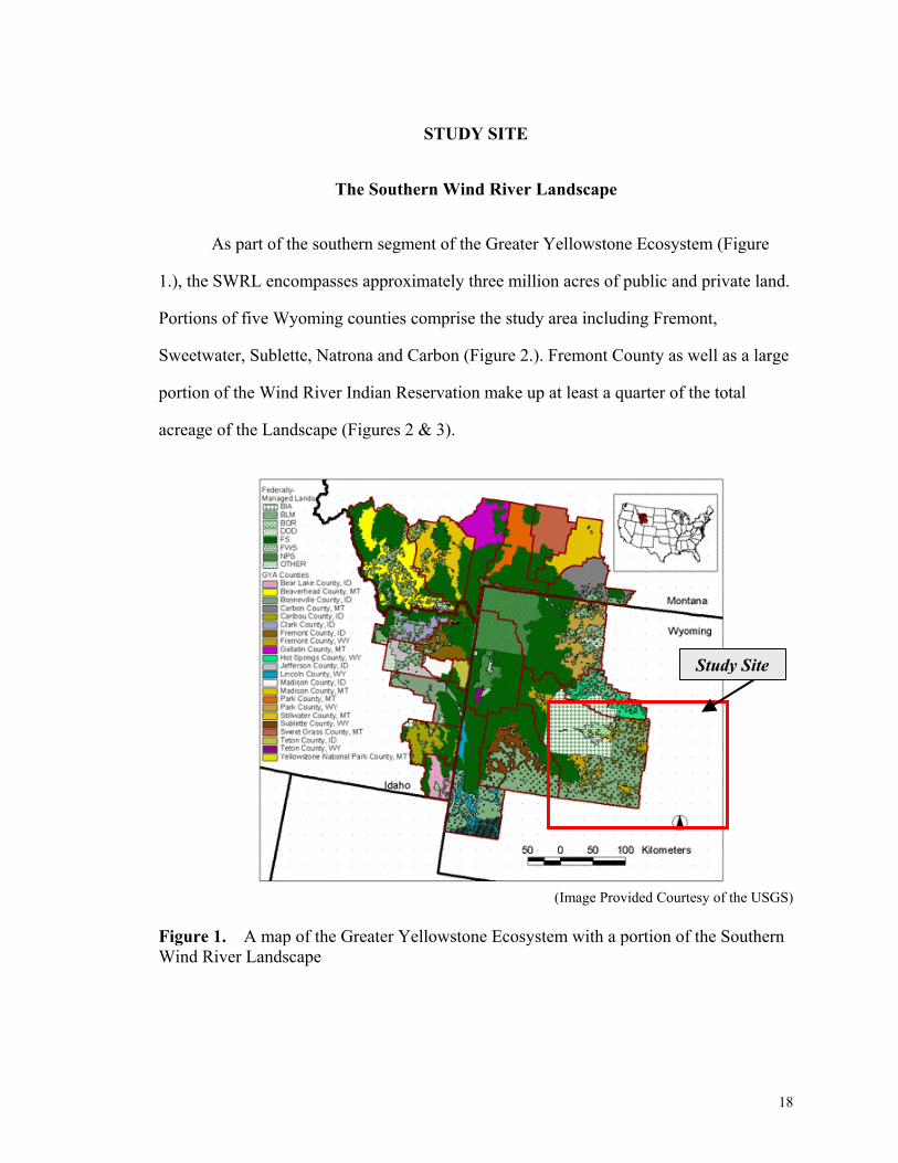
As part of the southern segment of the Greater Yellowstone Ecosystem (Figure
1.), the SWRL encompasses approximately three million acres of public and private land.
Portions of five Wyoming counties comprise the study area including Fremont,
Sweetwater, Sublette, Natrona and Carbon (Figure 2.). Fremont County as well as a large
portion of the Wind River Indian Reservation make up at least a quarter of the total
acreage of the Landscape (Figures 2 & 3).
(Figure 1)
Study Site
(Image Provided Courtesy of the USGS) Figure 1. A map of the Greater Yellowstone Ecosystem with a portion of the Southern Wind River Landscape
18
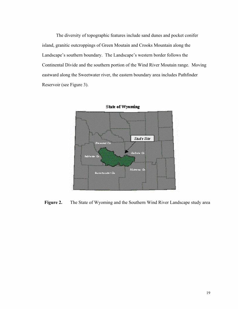
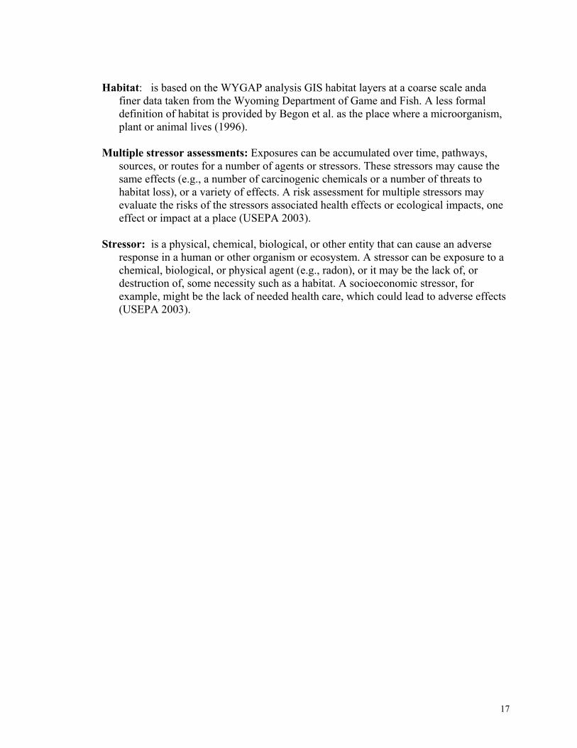
The diversity of topographic features include sand dunes and pocket conifer
island, granitic outcroppings of Green Moutain and Crooks Mountain along the
Landscape’s southern boundary. The Landscape’s western border follows the
Continental Divide and the southern portion of the Wind River Moutain range. Moving
eastward along the Sweetwater river, the eastern boundary area includes Pathfinder
Reservoir (see Figure 3).
Figure 2. The State of Wyoming and the Southern Wind River Landscape study area
19
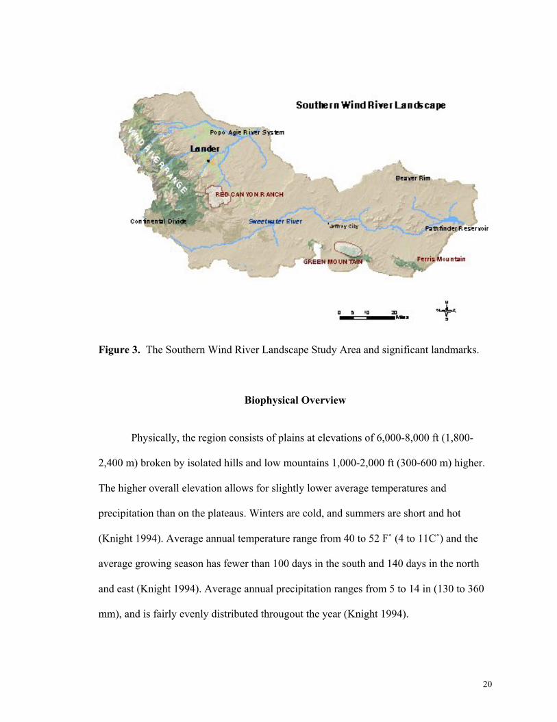
Figure 3. The Southern Wind River Landscape Study Area and significant landmarks.
Biophysical Overview
Physically, the region consists of plains at elevations of 6,000-8,000 ft (1,800-
2,400 m) broken by isolated hills and low mountains 1,000-2,000 ft (300-600 m) higher.
The higher overall elevation allows for slightly lower average temperatures and
precipitation than on the plateaus. Winters are cold, and summers are short and hot
(Knight 1994). Average annual temperature range from 40 to 52 F˚ (4 to 11C˚) and the
average growing season has fewer than 100 days in the south and 140 days in the north
and east (Knight 1994). Average annual precipitation ranges from 5 to 14 in (130 to 360
mm), and is fairly evenly distributed througout the year (Knight 1994).
20
Three major fourth order watersheds including the Popo Agie River complex, the
Sweetwater River, the Little Wind River and their related tributaries compose the
Landscape (Appendix A, Map #1). Major river systems and stream systems remain
undammed with the exception of some small high-elevation lake projects located along
first order streams. Much of the water is diverted for irrigation purposes throughout the
Landscape (TNC 2002). Large expanses of cropland along riparian corridors are
irrigated for winter feed and hay (TNC 2002).
Diversity among plant and animal communities is substantial. The ”ecoregion” of
the Intermountain Semidesert (Bailey 1995) is comprised primarily of a sagebrush steppe
ecosystem dominated by Artemisia tridentata and A. nova grasslands consisting of mostly
bunchgrasses including Koeleria macrantha, Poa secunda, Elymus spicatus, Oryzopsis
hymenoides, and Festuca (Fertig 1994). Of special concern to the BLM and The Nature
Conservancy are higher elevation, endemic and, particularly, cushion plant communties
located along the west and north slope of the Ferris Mountains and those located in the
Red Canyon area and the foothills of the Rattlesnake Mountains (Figure 4). Some
examples of these cushion plants include Yermo xanthocephalus (G1), Trifolium barnebyi
(G1), Cirsium aridum (G2), and Phlox pungens (G2) (Wyoming Natural Diversity
Database). For example, Wyoming’s only endangered plant species, Blowout
penstemon (Penstemon haydenii) are located along the southeastern boundary of the
Ferris mountains (WYNDD) in the study area (Figure 3).
A wide variety of willow and graminoid meadow communities exist along much
of the Sweetwater river and its tributaries (Fertig 1994). Alkali wetlands and subirrigated
ephemeral meadow plant communities are abundant throughout the landscape. Scirpus
21
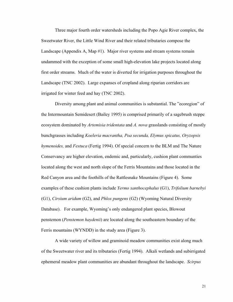
pungens/Distichlis stricta, Antennaria arcuata (G2) and Scirpus nevadensis (G4/S2) are
good examples of the rarer plants found in these unique areas.
(photo ourtesy of USGS) Figure 4. An example of vegetation representing the cushion plants found in the study area.
Other regions of interest identified for their unique vegetation communties
include the woodlands of limber pine and juniper along the Wind River Mountains and
foothill areas. Advances of pine blister into these important areas of critical deer and elk
wintering habitat are of particular concern as well as increased land development
including subdivisions around the Lander area. (Fertig 1994).
Additional important vegetation habitats include greasewood playas, the
calcareous grasslands in the southeastern portion of the Wind River Range, and the sand
dune system located near the Ferris mountains (Fertig 1994).
In addition, the granite desert mountains dotting the Sweetwater Plateau and
include the Ferris, Granite, Rattlesnake, Green and Grooks Mountains contain small
22
coniferous forest patches that are critical stopover sites for migrating birds and provide
seasonal habitat for other species.
Diversity in topographic features and vegetation contribute to a wide variety of
wildlife populations including the Townsend’s big-eared bat(Corynorhinus townsendii) ,
swift fox (Vulpes Velox), Grizzly bear (Ursus arctos), American peregrine falcon (Falco
peregrinus), Sage grouse, common species including elk and mule deer, and recent
residents like the grey wolf (Canis lupis) (WYNDD). River otters are found in the
Sweetwater river and its tributaries as well as mink. These waterways are also important
areas for several water bird species including the American avocet.
SocioEconomic Overview
Rough estimates for regional population place numbers at approximately 40,000
residents with 35,840 people residing in Fremont county alone (Bureau of Economic
Analysis 2000). Overall regional census data recorded an average 8.0 % increase in the
population from 1990 to 2000 for the five counties. The city of Lander is the most
populated community in the region with approximately 7,500 residents (Lander 2020
2000).
Primary land use in the region such as mining and ranching have deep historic
roots (TNC 2001). Agriculture, for example, contributes to the economic base for the
region and is the dominant land use on both public and private land, however, retail and
mining activity is by far the fastest growing industry (U.S. Census Bureau, Census 2000).
A 17.1% increase in Fremont County resident income was attributable to the mining
industry, for example (Wyoming State Department of Administration and Information –
Economic Analysis Division online). Mining activities like oil and gas development, coal
mining and support activities contribute to local economies but also to the state as well.
23
In addition, the service sector provides a significant proportion of the overal
earnings in the region. 25.7% of earnings in Fremont County are associated with the
service sector (Bureau of Economic Analysis 2000). Some of those services include those
associated with tourism and recreation including hunting, fishing, hiking and
backpacking.
Like most of the west, demographics in the intermountain west are changing.
According to the Lander Valley 2020 report cosponsored by the area Chamber of
Commerce, in 1994 18% of Lander’s population had arrived in the past three years.
According to the U.S. Population Census, Census 2000, 11.9% of Fremont County
residents had moved to the county from other states since 1995. In 1999, the Chamber
had reported a 600% increase in requests for information about Lander since 1990.
These changes in the social landscape are thought to be impacting the ecological
landscape. According to the American Farmland Trust (online), ranchland lands that
provide economic bases for rural communities are disappearing. Fremont County, in
particular, has been listed by the AFT in their report on Strategic Ranchlands as being of
their 25 “at risk” counties. As defined by AFT, strategic ranchlands at risk are those most
vulnerable to low density housing development by the year 2020. Fremont County was
targeted because of it’s projected growth in suburban density in the next twenty years.
The AFT methodology included identifying high quality agricultural land with desirable
wildlife characteristics including proximity to publicly owned lands, year-round water
availability, rural development densities and high diversity in vegetation cover types.
24

LITERATURE REVIEW
Applications of Bayesian statistics to risk assessment are found in medical
research and diagnostics and in ecological toxicology. Its applicability to wildlife
management occurs less frequently, but is no less appropriate. The following section
examines current literature addressing risk assessment, its applications, and the current
research and applications of Bayesian statistics and Bayesian networks to estimate risk in
light of scientific uncertainty. The terms Bayesian networks, Bayesian belief networks,
knowledge maps and probabilistic causal networks may be used interchangeably but
imply methods of reasoning using probabilities (Charniak 1991).
Risk Assessment
Ecological risk assessments are common methods of quantifying effects or the
likelihood of impacts from disturbance events and human related activities with respect to
ecosystem integrity. These analyses seek to identify, characterize or order a variety of
consequences that impact various ecological components, systems and/or functions.
According to Wilson and Crouch, risk assessments in general present a method of
examining risks “…so that they may be better avoided, reduced, or otherwise managed”
(1987: p. 268).
The Society for Risk Analysis (SRA) broadly characterizes the discipline of risk
analysis as including issues pertaining to risk assessment, risk characterization, risk
communication, risk management, and policy relating to risk (SRA online).
Furthermore, the analysis of risk considers threats from physical, chemical and biological
agents and from various human activities and natural events.
25

According to Hoffman et al. (1994), there are important differences between risks
that are voluntarily assumed and those that people are subjected to involuntarily.
Voluntary risks include those associated with activities we engage in linked with known
risk (e.g. driving a car, riding a motorcycle, smoking cigarettes). Involuntary risk are
those that may occur either to us or around us without prior consent including acts of
nature such as flood events, lightning strikes and exposure to environmental
contaminants. In addition, risks can be either statistically verifiable or nonverifiable.
Statistically verifiable risks can include either voluntary or involuntary activities that are
determined by direct observation. Statistically nonverifiable risks are only associated
with involuntary occurrences that are based on limited data sets, mathematical equations
and models (Hoffman et al. 1994).
Considerable research and applications of risk assessments have been completed
in a wide variety of disciplines where there is some level of uncertainty and limitations to
empirical data. In medical research, for example, a model derived empirically from
epidemiological studies is used to estimate the probability of a woman's developing
breast cancer over the next ten years. An initial assessment requires some level of data
collection to determine the “stressors'' (Hoffman et al. 1994). Here, certain factors are
known to be correlated with that form of cancer, such as the woman's age at first
childbirth, age at menarche, having a previous biopsy with atypical hyperplasia, and
others. However, not all stressors are the same type (e.g. chemical or genetic) and not all
data is available to quantify the risk (US EPA 2003).
Ecological risk assessment research, in particular, has been an important duty of
the U.S. Environmental Protection Agency. Substantial research conducted by the
26
agency pertains to toxicology and associated risks to the human health and to natural and
built environments. Chemical, biological, radiological, other physical, and even
psychological stressors can cause a variety of human health or ecological health effects.
Environmental related research include determining the measurable impacts from flood
events, point and non-point source pollution and erosion, all of which can provide data
that assist to guide scientists and land use managers in future land use planning (US EPA
2003).
Other efforts are directed towards community-based watershed risk assessments;
where, according to the EPA’s Guidelines for Ecological Risk Assessment (US EPA
1998b), three phases are necessary for risk assessment, including problem formulation,
risk analysis, and risk characterization. The agency’s overall approach to risk analysis
involves understanding risk, the sources of risk and the development of risk policy and
decision-making processes (Serveiss 2002).
Assessing the risk for these situations is quite methodological complex and
computationally challenging (EPA 2003). Probability-based assessments provide a
scientific process for estimating, with measurable degrees of certainty, anthropogenic
effects on the integrity of natural ecosystems (Cairns and McCormick, 1992). Suter
(1993) more clearly addresses the “certainty” issues with his definition of ecological risk
assessment as the determination of the probability of adverse effects on humans and
nonhuman biota resulting from an environmental hazard.
Russell and Gruber (1987) argue, however, that the EPA is placed in a difficult
position of assessing risks when a complete understanding of outcomes and risks are not
fully known. The National Research Council has stated that in any risk assessment,
27

inferences are derived from subjective scientific judgements and policy choices (National
Research Council 1983). Risk assessments provide guidelines but are not intended to
give certainty in a scientific sense (Gruber and Russell 1990). However, quantification of
risk is useful in approximating the magnitude of effect(s), to set conservation priorities
and to make comparisons (Gruber and Russell 1990).
Uncertainty is widely recognized and usually stated or assumed in research. The
American Heritage Dictionary (Morris 1978) defines uncertainty as “the condition of
being in doubt”. MacIntosh et al. (1994) defined the major types of uncertainty as
knowledge uncertainty and stochastic variability. Knowledge uncertainty is due to
incomplete understanding or inadequate measurement of system properties and is a
property of the analyst. Stochastic variability is due to unexplained random variability of
the natural environment and is a property of the system under study (Hession et al. 1996).
Uncertainty is acknowledged in risk assessments of population viability, in
methods of determining conservation status, in land management decisions and in
conservation of biodiversity. Akcakaya and Raphael (1998) conducted a risk assessment
where the viability of the northern spotted owl was estimated with respect to human
impacts. The authors demonstrate the effect of uncertainty resulting from a lack of
information and measurement error on the assessment. The research parameters or
measurements consider the risk of decline in the metapopulation and the estimated time
to extinction. According to Akcakaya and Raphael, if uncertainty is incorporated in the
research, parameterized and used to estimate upper and lower bounds of species viability,
assessing human impacts is reliable. The results, they concluded, are sensitive to large
28
uncertainties related to habitat loss as well. Overall, the predictions were affected by the
uncertainties in inputs and were relative to the sets of assumptions or scenarios.
According to Todd and Bergman (1998), assessing threat(s) to a species does not
account for the “underlying uncertainty inherent in the data”. They consider that
uncertainty in the parameter estimates of the biological variables can be used within
reasonable bounds to make plausible determinations of species status.
Bayesian Statistics and Bayesian Networks
Bayesian networks model uncertainty by “explicitly representing the conditional
dependencies between different knowledge components. It provides an intuitive
graphical visualization of the knowledge including the interactions among the various
sources of uncertainty” (Pearl 1988). The Bayesian approach to incorporation of expert
belief, probabilistic inference, prior knowledge and numeric information (Varis 1995)
allow for a risk assessment to account for uncertainty.
Uncertainty arises in a variety of situations such as: (1) uncertainty in the experts
themselves concerning their own knowledge; (2) uncertainty inherent in the domain
being modeled; (3) uncertainty in the knowledge being translated; and, (4) uncertainty of
the accuracy and actual availability of knowledge. Bayesian networks use probability
theory to manage uncertainty by explicitly representing the conditional dependencies
between the different knowledge components (Varis 1995). This provides an intuitive
graphical visualization of the knowledge including the interactions among the various
sources of uncertainty.
Applications
29
The essence of Bayesian statistics and Bayesian belief networks is Bayes’
Theorem. Bayes’ Theorem is the fundamental law governing the process of logical
inference-determining degrees of confidence we have in various possible conclusions,
based on a body of available evidence. This is exactly the process of predictive
reasoning; therefore, to arrive at a logical defensible prediction one must use Bayes’
Theorem (Bayesian Systems, Inc. online). The difference between what Bergerud and
Reed (1998) call frequentist statistics and Bayesian statistics is the way parameters are
defined. A frequentist’s approach would have one or more unknown parameters and the
Bayesian approach assigns probabilities to parameter values before the study is
conducted.
In forest management, for example, Bergerud and Reed (2002) contend that
managers would like simple answers to practical questions from traditional scientific
methods of experimental and/or observational sampling. For example, frequentist
statistical methods can not “directly” provide an assessment of the probability that one or
more hypotheses are true, or the probability that an estimate of a parameter is close to its
unknown true value. Such results are of limited use to managers. However, a Bayesian
method can provide precisely this type of information (Bergerud and Reed 1998).
In it’s essence, Bayes’ Theorem provides a basis to assess how people use
empirical observations or experience to update the probability that a hypothesis is true
(Bergerud and Reed 1998) . This is also called “posterior odds” and can be represented
as the following mathematical statement.
P(H) = The probability you would have assigned to the hypothesis before you made the observation, called the “prior probability” of the hypothesis.
P(O|H) = The probability the observation would occur if the hypothesis were true.
30
P(nonH) = The prior probability the hypothesis is not true, 1-P(H)
P(O|nonH) = The probability the event would have occurred even if the hypothesis were not true.
P(H|O) = P(H) x P(O|H) / [P(H) x P(O|H) + P(nonH) x P(O|nonH)]
Variations of Bayesian statistics are used in ecological research. For example,
Dilks et al. (2002) used the Bayesian Monte Carlo (BMC) analysis to quantify
uncertainty in a water quality model for Lake Okeechobee located in south Florida.
Bayesian inference has been combined with Monte Carlo analysis to generate improved
estimates of parameter uncertainty by considering the variations in parameter values to
describe the observed data (Dilks et al. 1992). By combining prior information (prior
probabilities) derived from literature reviews with available site-specific data set ranges,
the BMC was used to describe a given model simulation output. The results fell within
the 95% confidence interval of the observed total data (Dilks et al. 1992). Additional
analysis included projections for model uncertainty given different future scenarios.
Additional, applications of Bayesian statistics in ecology include modeling of
neotropical bird habitat. Vitale (online) applied GIS with landscape variables and
Bayesian statistics where multiple hypotheses are represented as probabilities rather than
accepted or rejected. The output was a map of probability of species occurrence that was
similar to habitat suitability and association maps (Vitale online). The assertion in this
project is that stakeholders can easily understand the creation of a map using Bayesian
statistics; and, that rather than being a definitive determination of habitat, the estimates
are probabilities or likelihoods of habitat presence. This is an implicit statement of
31
uncertainty and allows for stakeholder input for management development (Wade 2000
in Vitale online).
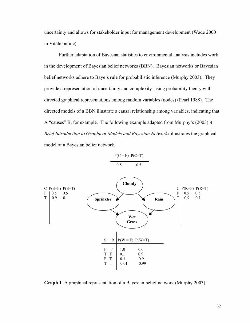
Further adaptation of Bayesian statistics to environmental analysis includes work
in the development of Bayesian belief networks (BBN). Bayesian networks or Bayesian
belief networks adhere to Baye’s rule for probabilistic inference (Murphy 2003). They
provide a representation of uncertainty and complexity using probability theory with
directed graphical representations among random variables (nodes) (Pearl 1988). The
directed models of a BBN illustrate a causal relationship among variables, indicating that
A “causes” B, for example. The following example adapted from Murphy’s (2003) A
Brief Introduction to Graphical Models and Bayesian Networks illustrates the graphical
model of a Bayesian belief network.
P(C = F) P(C=T)
0.5 0.5
C P(S=F) P(S=T) C P(R=F) P(R=T) F 0.5 0.5 F 0.5 0.5 T 0.9 0.1 T 0.9 0.1
S R P(W = F) P(W=T)
F F 1.0 0.0 T F 0.1 0.9 F T 0.1 0.9 T T 0.01 0.99
Cloudy
Sprinkler Rain
Wet Grass
Graph 1. A graphical representation of a Bayesian belief network (Murphy 2003)
32
The application of Bayesian belief networks in ecology has proven useful in
assessing and managing wildlife species (Cohen 1988, cited in Marcot et al. 2001) and
for forests (Crome et al. 1996, cited in Marcot et al. 2001). Researchers in the U.S.
Forest Service’s Pacific Northwest Research Station have applied Bayesian belief
networks to evaluate fish and wildlife population viability under various land
management alternatives (Marcot et al. 2001).
Important elements contributed to the thoroughness of this multi-level analysis
including access to significant data sources, participation of numerous experts and the
various extents to which the analyses were conducted. The first element included the
geographic extents at which the analyses were conducted. These included a basin-wide
level (specifically the Columbia River basin) a subwatershed level, and a site-specific
analysis. For example, at a subwatershed level, GIS data depicted wildlife habitats at 1
km2 pixel resolution and key environmental correlates (Marcot et al. 2001) such as
specific species-environment relations and expert review. At a basin-wide extent, the
analysis outcomes represented the potential population(s) responses to the management
strategy. Empirical data was readily available through two substantial databases, one
developed for the Interior Columbia Basin Ecosystem Management Project and the other
published databases. The research team also had extensive multi-year input from a large
panel of experts (80+) who collaborated in a Delphi process (Marcot, personal
communication 2002).
In this particular application of BBN’s, influence diagrams using conditional
probability tables represented the causal relations among ecological factors that influence
likelihood outcomes or effects given some land management strategy (Marcot et al.
33

2001). According to Marcot et al., (2001) the BBN species models provide a method for
expressing the ecological cause and effect relationship influencing a species and the
uncertainty inherent in that relationship. Uncertainty in the BBN is found in the
probability distributions for each node (variable), the error denoted by the mean standard
deviation and the sensitivity of nodes to another. Finally, according to Marcot et al.,
(2001) the BBN models should provide synthesis of expert opinion and experience with
solid data. “They should also provide a basis for understanding the types, sources,
degrees, and implications of uncertainties in existing data and expert understanding.”
Other work in BBN applications has been completed by Hass and Cleaves
(online) to model waterbody eutrophication and by Kuikka and Varis (1997) to assess the
Baltic salmon. Kuikka and Varis (1997) utilize a Bayesian meta-model as a diagnosis
and forecasting method for allowing “fusion” of other analyses such as regression and
Virtual Population Analyses that facilitate probabilistic predictions in a Bayesian belief
network. Their work provides a complete description of how the BBN is created (e.g.
what the nodes contain, prior and posterior probability distributions, and the links
between nodes), how the network is propagated, and how uncertainty and contradictory
information are contained in an analytic framework (Kuikka and Varis 1997).
Kuikka and Varis continue to assert that the three most crucial properties of this
approach are: (1) the advanced handling of uncertainties that include network
propagation and presentation, objectives and structure; (2) the ability to include modeling
techniques from many methodologies typically considered divergent such as metric and
linguistic; and, (3) support for the acquisition of expert knowledge and structure of a
34
model. Final recommendations suggest that expert opinion and knowledge should be
handled more formally as they are often important sources of information.
Lynam et al. (2002) applies Bayesian belief models to adaptive resource
management strategies in Zimbabwe. The model was adapted to incorporate natural and
social dynamics with environmental research to improve community involvement in the
decision-making process. Spatially and temporally complex variables such as the
dynamics in land change were a key component of the Bayesian network model. Local
village representatives offered their feedback about the cause and effect relationships
between the model variables and their management actions in relation to the subsequent
impacts on the community. By identifying problems in the system dynamics modeling,
the local community took direct action to stop particular activities including illegal
allocation of lands (Lynam et al. 2002).
Conclusion
Two general conclusions can be made from the literature on both risk assessment
and Bayesian belief networks: scale and extent matters and uncertainty must be formally
accounted for. Risk assessments are established to further our management objectives. In
applying assessment results to land use and ecological management and decision-making,
risk assessment “is often characterized by a large number of uncertain, interrelated
quantities, attributes and alternatives based on information of highly varying quality” (US
EPA 2003: p. 129). When dealing with ecological risk assessment, particularly those
concerned with population viability and habitat-species associations, there are often
problems in the geographic extent, the physical and temporal scales as well as the amount
35
and quality of observation data, purely physical or data-based models to be used as
effective decision-making tools. Available data is either too broad or fine for the
question at hand. Furthermore, the collection of statistically valid data may often prove
impossible, or at least highly impractical, due to the nature and extent of the problems
and with the resources available for research. Bayesian statistics seems to provide a
reasonable method to parameterize input variables given inconsistencies in existing data
sources with an opportunity to apply expert knowledge.
Futhermore, the process of environmental decision-making does not support
quantification of decision inputs and inference, bias and opinion is typically assumed
(Serveiss 2002). Bayesian approaches to risk assessment and environmental management
may provide a method of accounting for expert and stakeholder knowledge (Serveiss
2002).
36
METHODS
The project was conducted in three stages. In the first stage, relevant spatial data
were collected and processed for risk assessment integration. In the second stage, the
Bayesian network-based risk models derived from expert opinion were developed to
provide the framework and rationale for the final risk maps. The third and final stage
was the integration of GIS with the BBN risk models to create the risk maps.
Project Parameters
Spatial and temporal considerations were identified as parameters for creating a
risk network. First, data availability was a limiting factor. Both spatial and empirical
data were limited for the study area. As a result, not all variables, particularly temporal
data influencing habitat such as climatic fluctuations were considered. Available spatial
data representing human activity were limited in the study area; therefore, data layers, in
general, are coarse and were often adapted to characterize broad anthropogenic influence
patterns and species’ seasonal habitats.
The project sought to represent the spatial distribution of risk with respect to
habitat at two spatial extents illustrating the application of the BBN framework to both
landscape and site-specific risk assessments. Two approaches to spatial data assessment
were conducted. 30-meter GIS data were adequate for illustrating the landscape or
regional extent of risk with respect to habitat for the entire study area. A second
approach identified two sites nested within the Landscape that are representative of
unique vegetation associations.
37

The second parameter was time availability. As a result, risk effect analyses were
not completed as part of the risk assessment. Therefore, the assessment is broad and
solely addresses the spatial patterns of risk at landscape and site-specific levels.
Data Collection
GIS data were collected for the study site from numerous public sources including
the Bureau of Land Management, the State of Wyoming Geographic Information Center,
The Wyoming Natural Diversity Database, and The Nature Conservancy. Relevant data
included land ownership, a 30- meter digital elevation model, mineral development
potential and other surface feature information including pipelines, oil and gas well sites,
mine sites, roads and fences.
Habitat data layers were critical to the assessment. Standard 30-meter data were
readily accessible. At a landscape or regional extent, these course resolution data are
sufficient to represent generalized landscape pattern, habitat distribution, and the spatial
dispersion of human-related features.
Those data associated with human activities or disturbances were buffered to
portray the relative spatial disturbance of particular features (Figure 3.) This
determination was based on expert knowledge of the features, impacts on habitat and
known understanding of avoidance behavior of a particular species. Well pads were
given three concentric buffers with distances of 0 – 100 meters from the well pad, 100 –
300 meters and 300 – 500 meters. Linear features such as roads, fences, and pipelines
were buffered 30 meters on either side.
38
Coarse level
The coarse resolution habitat data were obtained from the Wyoming GAP
analysis completed in 1996. Thirty-meter land cover classification assessment
delineated habitat potential for the three species of interest. Potential habitat for mule
deer and sage grouse covered the entire study area while mink habitat was located
primarily along riparian corridors and extending into the uplands.
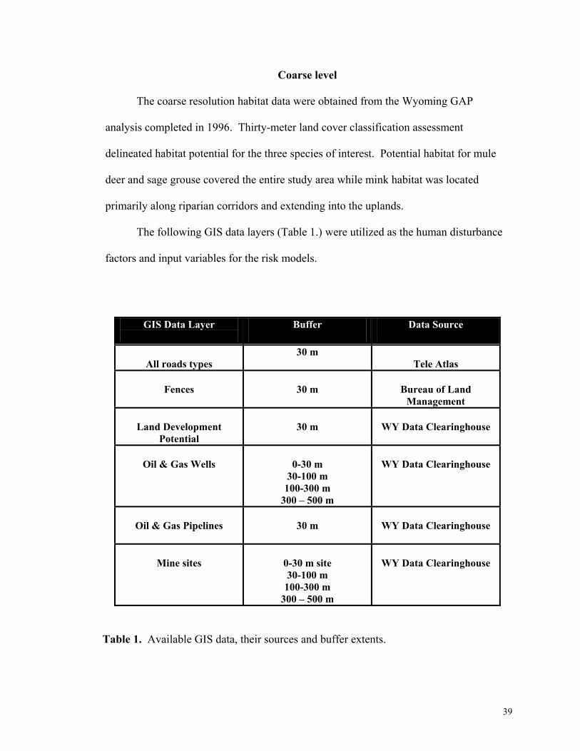
The following GIS data layers (Table 1.) were utilized as the human disturbance
factors and input variables for the risk models.
GIS Data Layer
Buffer Data Source
All roads types
30 m Tele Atlas
Fences
30 m
Bureau of Land
Management
Land Development Potential
30 m
WY Data Clearinghouse
Oil & Gas Wells
0-30 m
30-100 m 100-300 m
300 – 500 m
WY Data Clearinghouse
Oil & Gas Pipelines
30 m
WY Data Clearinghouse
Mine sites
0-30 m site 30-100 m
100-300 m 300 – 500 m
WY Data Clearinghouse
Table 1. Available GIS data, their sources and buffer extents.
39
Fine Level
The site specific or fine level assessment included identifying species’ seasonal
habitat. The Wyoming Department of Game and Fish (WYGF) provided the finer scale
seasonal habitat information for both mule deer and sage grouse, while mink seasonal
habitat spatial data were not available. The site-specific data provided a finer level of
detail relative to the disturbance. Often, differentiation in habitat type (e.g. sage grouse
reproduction areas such as leks and nesting sites vs. winter habitat) may require unique
treatment in a GIS environment. For instance, the buffer of a given seasonal habitat may
be larger compared to another seasonal habitat site for the same species.
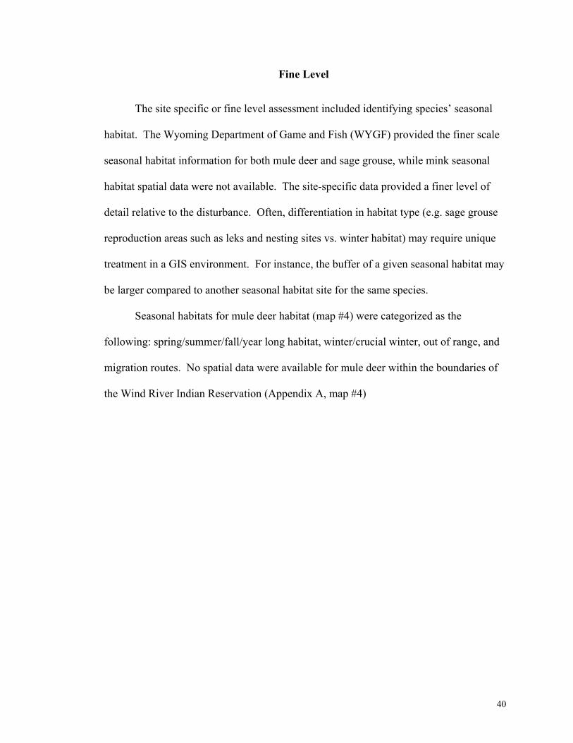
Seasonal habitats for mule deer habitat (map #4) were categorized as the
following: spring/summer/fall/year long habitat, winter/crucial winter, out of range, and
migration routes. No spatial data were available for mule deer within the boundaries of
the Wind River Indian Reservation (Appendix A, map #4)
40
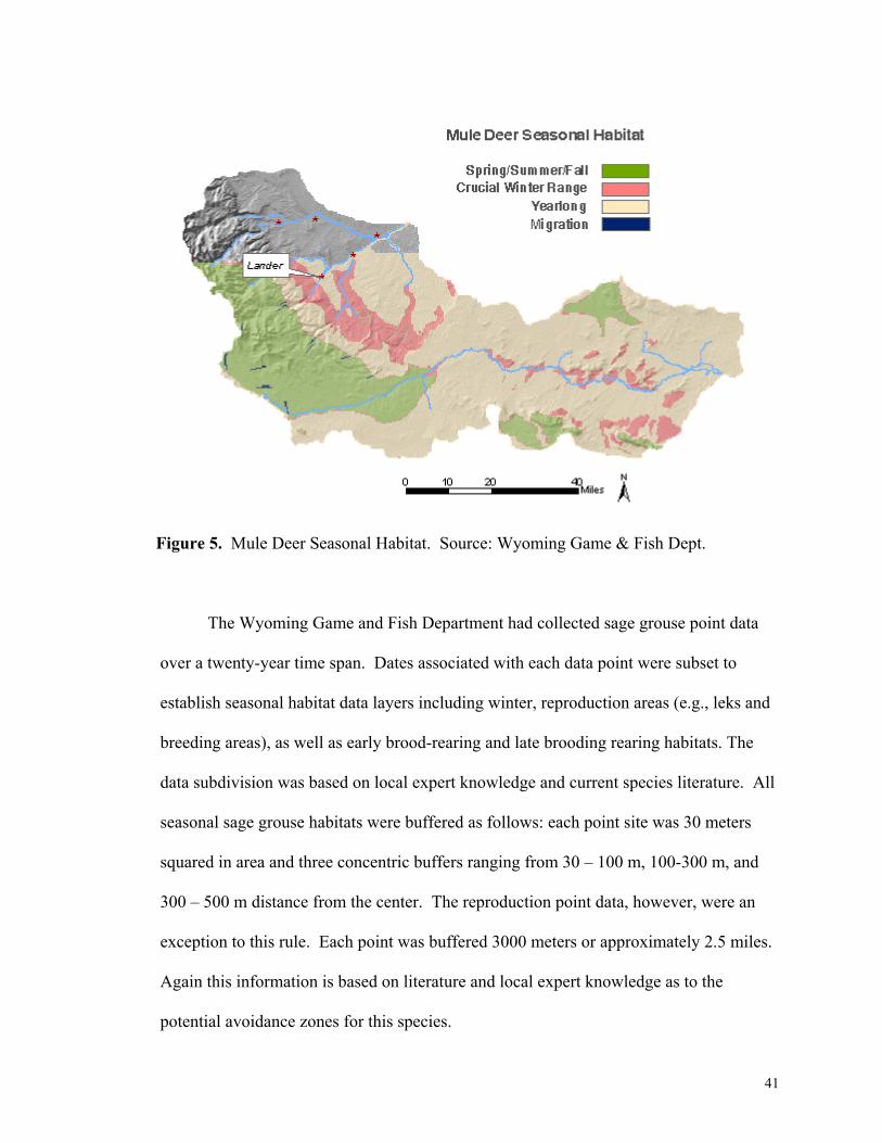
Figure 5. Mule Deer Seasonal Habitat. Source: Wyoming Game & Fish Dept.
The Wyoming Game and Fish Department had collected sage grouse point data
over a twenty-year time span. Dates associated with each data point were subset to
establish seasonal habitat data layers including winter, reproduction areas (e.g., leks and
breeding areas), as well as early brood-rearing and late brooding rearing habitats. The
data subdivision was based on local expert knowledge and current species literature. All
seasonal sage grouse habitats were buffered as follows: each point site was 30 meters
squared in area and three concentric buffers ranging from 30 – 100 m, 100-300 m, and
300 – 500 m distance from the center. The reproduction point data, however, were an
exception to this rule. Each point was buffered 3000 meters or approximately 2.5 miles.
Again this information is based on literature and local expert knowledge as to the
potential avoidance zones for this species.
41
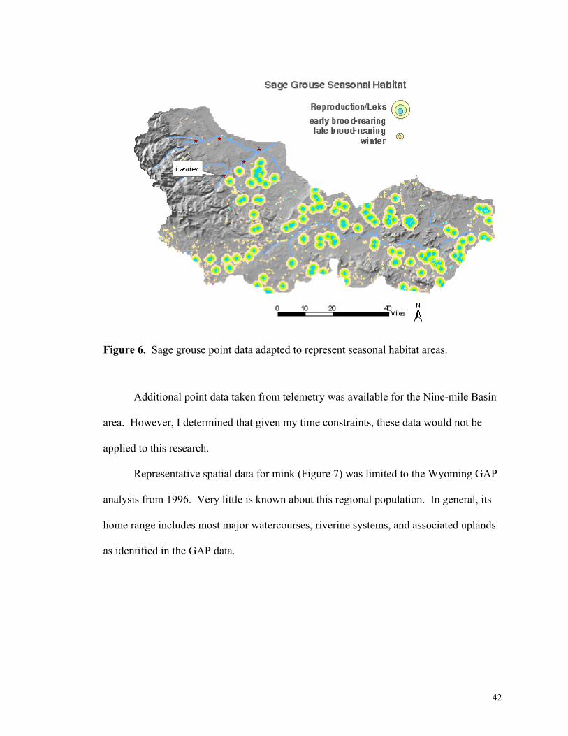
Figure 6. Sage grouse point data adapted to represent seasonal habitat areas.
Additional point data taken from telemetry was available for the Nine-mile Basin
area. However, I determined that given my time constraints, these data would not be
applied to this research.
Representative spatial data for mink (Figure 7) was limited to the Wyoming GAP
analysis from 1996. Very little is known about this regional population. In general, its
home range includes most major watercourses, riverine systems, and associated uplands
as identified in the GAP data.
42
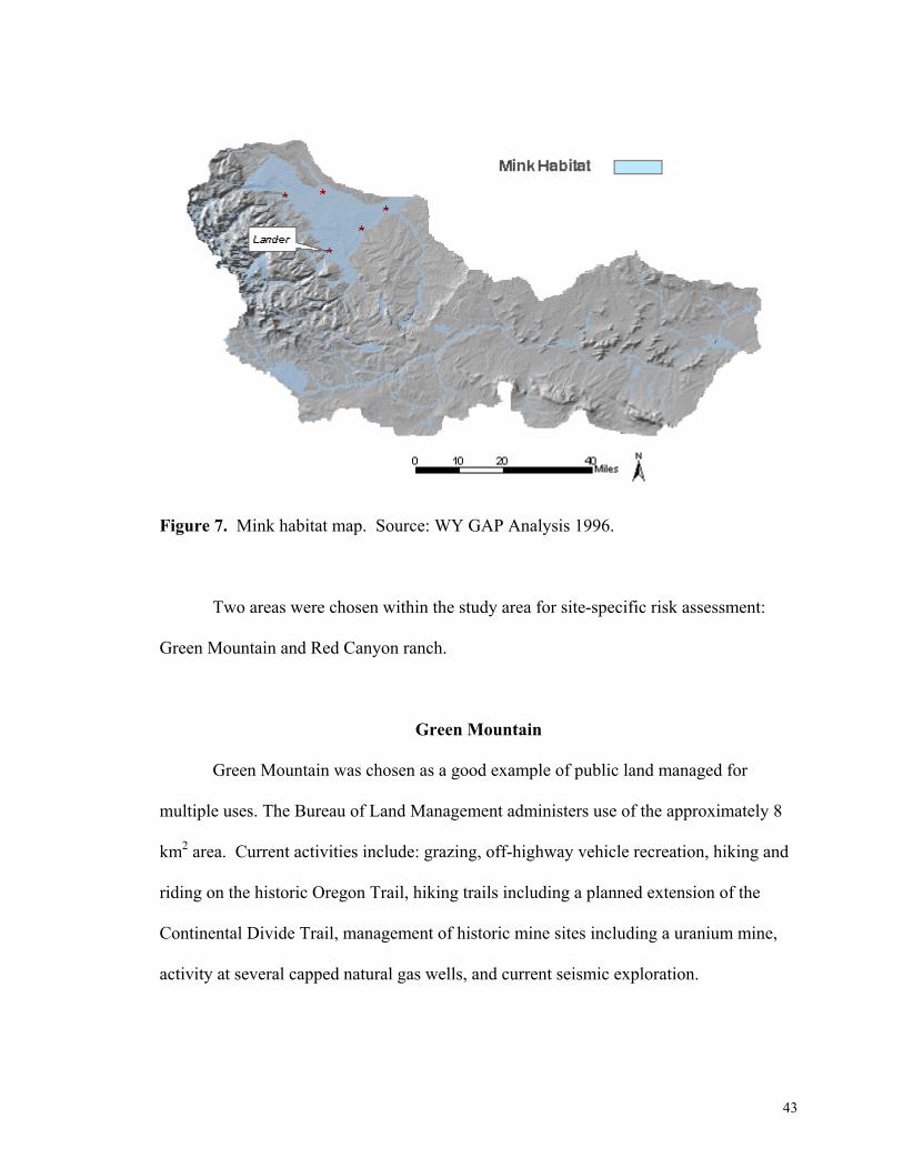
Figure 7. Mink habitat map. Source: WY GAP Analysis 1996.
Two areas were chosen within the study area for site-specific risk assessment:
Green Mountain and Red Canyon ranch.
Green Mountain
Green Mountain was chosen as a good example of public land managed for
multiple uses. The Bureau of Land Management administers use of the approximately 8
km2 area. Current activities include: grazing, off-highway vehicle recreation, hiking and
riding on the historic Oregon Trail, hiking trails including a planned extension of the
Continental Divide Trail, management of historic mine sites including a uranium mine,
activity at several capped natural gas wells, and current seismic exploration.
43
Red Canyon Ranch
Red Canyon Ranch is an ~4,600 acre property owned by The Nature Conservancy
with an additional 30,000 + acres of federally permitted land and state wildlife
management inholdings. Like Green Mountain, the Red Canyon area is unique in its
plant and animal diversity. Significant aspen stands, rare plant communities, and wildlife
populations occupy the site. Surrounding land conversion from traditional large
agricultural production to smaller, subdivided ranchettes are of concern and impact local
biodiversity. The site is representative of the larger regional pressures from rural land
development activities including further road development and off-highway vehicle
access into more remote areas, domestic pets that may threaten wildlife populations, and
general degradation of habitat through the loss of food and water sources, cover and loss
of adequate space required for reproduction and survival.
GIS is intended to visually represent patterns of disturbance in the landscape
relative to habitat. With the addition of identification of risk areas using Baysean Belief
Networks, the maps can be used to illustrate habitat/wildlife experts understanding of risk
and to graphically depict that understanding. The benefit of this process is intended for
regional planning and management efforts. Using maps and models, collaborative
planning groups can confirm or reject the expert knowledge or understanding of risk as
well as determine how to plan for future development and identify needs for further
analysis.
Bayesian Networks
The use of the term Bayesian belief network as applied to this research refers to a
probabilistic model connecting independent variables with conditional statements that
define variable interdependence or a causal links between variables. In this case, BBN’s
44

will be used to model the probabilities of risk from human disturbance to wildlife habitat.
Two stages in the risk modeling process were completed to attain the habitat risk
assessments. The first stage was to build the model by determining the prior probabilities
using available GIS data and expert knowledge. The second involved interviewing
experts to rank risk for determination of the posterior probabilities. The posterior
probability in this case is an estimation or approximation of risk probability given the
presence of habitat type and the rankings of risk relative to a surface feature or
disturbance type. For example, the probability of risk being ‘high’ is determined by the
presence of a sage grouse lek site in proximity to a road or well pad. The prior
probability would be if habitat or a feature is present conditioned by the expert judgement
estimation of risk or called the conditional probability.
The belief network is designed to illustrate the believed relations between sets of
variables relevant to some question (Norsys, online). Relevancy is based on
observations, knowledge or empirical evidence. The first step in building the network for
this risk assessment was determining the variables believed to influence or pose risk to
wildlife habitat and those data that are spatially represented. Those activities include:
1. Land ownership. Land use development includes proposed or established housing and commercial developments, and management or changes of agricultural lands.
2. Oil and gas development and associated pipeline and pad systems. 3. Roads and road density including those classified as either primary,
secondary, two-track, off-road vehicle or trails.
Risk Model Development: Application of the Bayesian network
45

A risk assessment can be divided into three critical steps. Formalizing the process
includes: 1) risk identification, 2) risk estimation and 3) risk evaluation. For this project,
risk identification uses local expert knowledge to identify the human-related activities
within the study area that pose risk to either mule deer, sage grouse or mink habitat. In
an interview, those same experts are asked to rank or estimate the risk relative to a
particular habitat. The third and final step includes both landscape and site-specific risk
evaluations using a Bayesian belief network that are subsequently spatially represented.
Netica
The belief networks for each species were built using the Netica software
package by Norsys, Inc.. These networks model an outcome of disturbance defined in
terms of an ordinal scale of high, medium , low, unsure, or no. To build each model,
prior (unconditional) probabilities must be established. That is, what is the likelihood that
an input parameter (e.g., roads or habitat) is in a particular state (e.g., present or not
present). My selected variables represented available spatial information but not all
possible variables contributing to a risk model . In this case, prior probabilities were
established in the initial phase of the interviewing process where experts are asked to
determine which human-related activities pose risk to a particular habitat.
The GIS proxies such as habitat, roads, and wells are quantified or ordinally-
scaled variables portrayed as nodes within the network. Sets of nodes represent distinct
model elements such as seasonal habitat and selected human activities. Prior probability
and conditional probability nodes describe the cause and effect relationship between
variables that influence habitat (Marcot 2001). Additional information for determining
46
the state of a variable was taken from literature and by regionally-based species’ experts
through an interview process.
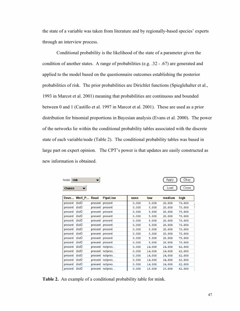
Conditional probability is the likelihood of the state of a parameter given the
condition of another states. A range of probabilities (e.g. .32 - .67) are generated and
applied to the model based on the questionnaire outcomes establishing the posterior
probabilities of risk. The prior probabilities are Dirichlet functions (Spieglehalter et al.,
1993 in Marcot et al. 2001) meaning that probabilities are continuous and bounded
between 0 and 1 (Castillo et al. 1997 in Marcot et al. 2001). These are used as a prior
distribution for binomial proportions in Bayesian analysis (Evans et al. 2000). The power
of the networks lie within the conditional probability tables associated with the discrete
state of each variable/node (Table 2). The conditional probability tables was based in
large part on expert opinion. The CPT’s power is that updates are easily constructed as
new information is obtained.
Table 2. An example of a conditional probability table for mink.
47
Expert Knowledge
The primary objective in the interview process is to determine, from resource
professionals, a cause and effect relationship between human-related activities and
species habitat. The process was adapted from Marcot et al.’s (2001) research in
Bayesian belief network modeling of wildlife population viability in the Columbia River
Basin. Their research utilized a Delphi process in which wildlife professionals estimated
a causal web influencing wildlife populations given an environmental impact statement’s
land management alternatives. This process resulted in probabilities of population
viability and likelihood of management effects (Oliver and Smith 1990). Over 80 wildlife
professionals were available for the Delphi and “selected at-risk fish and wildlife species”
(Marcot 2001). I determined that due to time constraints and logistics associated with
travel and commitments with wildlife experts, that an informal, personal interviews
would provide sufficient baseline data for establishing model variables and ranges or
states for the variables.
Interview Selection criteria
Two experts per species were selected to establish a-priori probabilities for the
risk assessment. These individuals were recognized among their peers as having
significant species and-or habitat specific knowledge and experience. They were either
state or federal resource professionals identified as having a working knowledge of the
region or had worked within the region of interest. Because the majority of the land is
managed by federal and state resource agencies, these professionals were selected
because of their familiarity with agency management issues and specific wildlife
populations in the region.
48
Interview Methodology
A semistandardized (Berg 2001) approach was used for the personal interview
with selected wildlife professionals. According to Berg (2001), a semistandardized
method, as compared to a standardized approach, allows for a freer discourse between
interviewer and interviewee. In a standardized format of interviewing, the questions are
rigidly outlined and therefore do not allow for clarification or probing of answers. The
interviewer’s use of language and terminology may differ from that preferred and utilized
by these particular professionals. The semistandardized approach allows the researcher
to further delve into subject material or to digress to previous issues so as to supplement
and improve the understanding of the content of information obtained.
In this research, the semistandardized method was particularly useful because the
prior probabilities and marginal probabilities of the model are established by the initial
interview session. For example, establishing whether or not sage grouse habitat is at risk
from road networks depended on interview responses. Depending on the response, the
researcher may continue to probe regarding: a) what the professional believes or
understands the causes of risk to sage grouse habitat to be; or b) what specific aspects of
roads and road networks create risk to sage grouse habitat.
Freeform probing can allow for clarification of interpretations of observations and
of scientific literature. Due to the probabilistic nature of the BBN habitat risk model, it is
important that information is clearly represented within the model and in the model
structure. How and to what degree interpretations of information that includes personal
observations, anecdotal information and scientific literature is articulated is critical to risk
modeling. It is the wildlife professionals’ responses to these questions and the
49
information they provide that reflect the basis on which land managers rely when creating
and updating land and wildlife management plans.
The semistandardized interviewing method was comprised of scheduled questions
leading to unscheduled or probing questions, whereby a professional’s perceptions were
more fully detailed (Berg 2001). (See appendix B).
Risk Models Three steps occur in the development of the risk models. First, following the
interview process, expert responses are rated on a numerical scale. For instance, ‘High’
risk ranged in value from .68 - 1; ‘Medium’ risk = .34 - .67; ‘Low’ risk = .17 - .33; and,
a ‘None’ risk ranking = 0 - .16.
One challenge in this process is to combine multiple expert opinions for a ranking
range. To meet this challenge, Marcot et al. (2001) used a consensus building process to
establish risk rankings. In this project, ancillary data were used to weight individual
responses and to establish a relative average value. For example, current literature that
supports or counters the respondent rankings would influence the final value. In addition,
respondent qualification of rankings such as dependency on activity location, utilization
and age would also influence the final value.
The second step applies these values in establishing the conditional probability
tables (CPT) within the Netica software. An influence diagram is created that symbolizes
the variables that pose risk to habitat (Graph 2). For example, given the presence or
absence of a particular activity (e.g. well pad), the probability of risk is established from
50
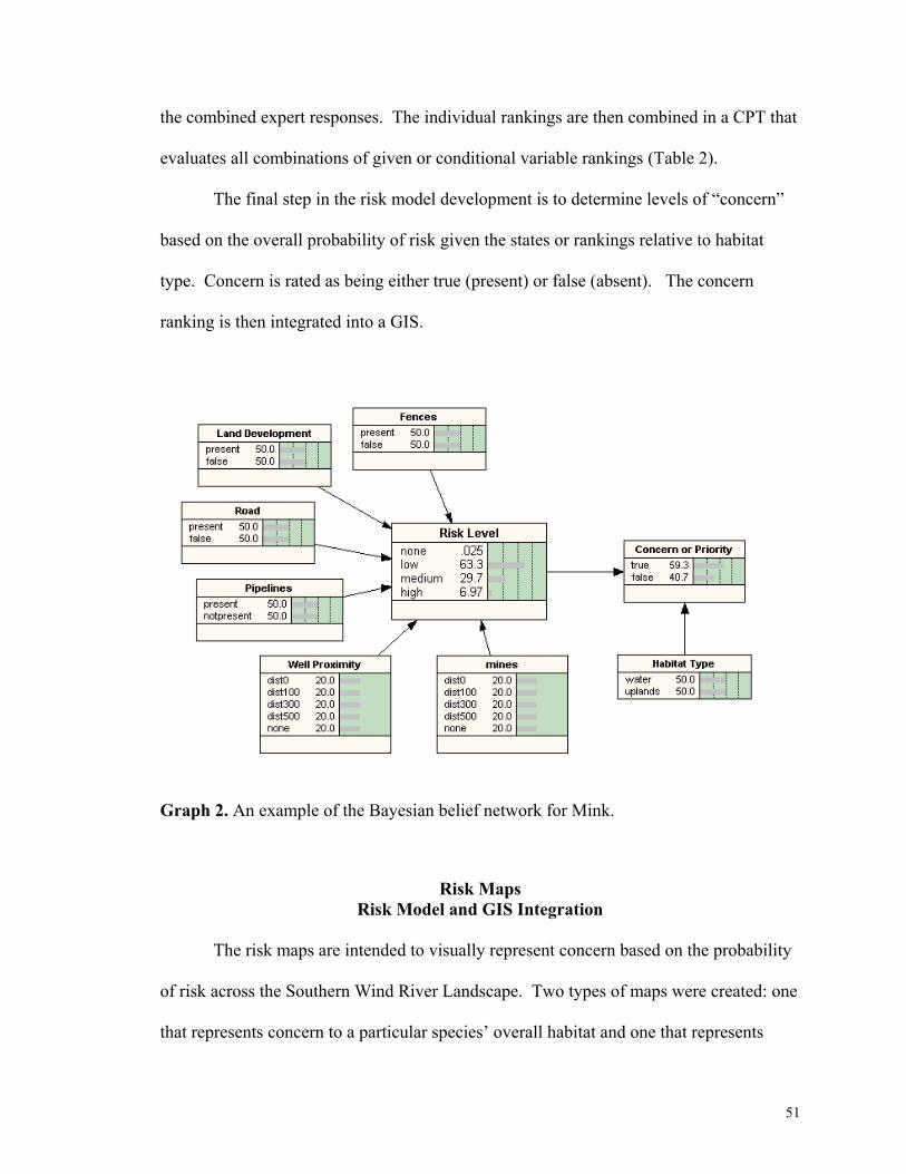
the combined expert responses. The individual rankings are then combined in a CPT that
evaluates all combinations of given or conditional variable rankings (Table 2).
The final step in the risk model development is to determine levels of “concern”
based on the overall probability of risk given the states or rankings relative to habitat
type. Concern is rated as being either true (present) or false (absent). The concern
ranking is then integrated into a GIS.
Graph 2. An example of the Bayesian belief network for Mink.
Risk Maps Risk Model and GIS Integration
The risk maps are intended to visually represent concern based on the probability
of risk across the Southern Wind River Landscape. Two types of maps were created: one
that represents concern to a particular species’ overall habitat and one that represents
51
concern to that species’ seasonal habitat. The following section describes in the step-by-
step process of how the risk model outcomes or concern rankings are integrated in a GIS
environment.
First, each of the existing data layers are converted to a grid format. Each grid
cell is given a value. For example, in the mink habitat grid, habitat presence = 1 and
habitat absence = 0. Sage grouse data and mule deer habitat are unique in that each
habitat type is given a value based on seasonal habitat delineation. There are five habitat
types identified for mule deer: crucial winter habitat = 5, migration routes = 4, yearlong =
3, spring/summer/fall = 2, out-of-range (Wind River Indian Reservation) = 1 and no data
(outside of the study area) = 0. Sage grouse habitat types are distinguished similarly:
lek/reproduction areas = 4, early brood-rearing = 3, late brood-rearing = 2, wintering
habitat = 1 and no data = 0.
An empty grid is created with the same spatial extent as the study site boundary.
A computer program or “risk program” written in Visual Basic “steps through” each of
the existing habitat grid cells and identifies the state of each disturbance or range of risk
probability in that particular cell. For instance, if a habitat grid cell = 4, the risk
probability state may equal .57. The risk program will take those states and enter them as
evidence in the Bayesian network. The program will then compute the following ranges
using the BBN and probability distribution of the risk node yielding:
1. P(C=H) (the probability of Concern = high)
2. P(R=M) (the probability of Concern = medium)
3. P(R=L) (the probability of Concern = low)
4. P(R=none) (the probability of Concern = none)
52

The risk program will store the concern rankings in the grid cells of the new grid.
The final step is to convert the grids to images with color schemes that signify the ranges
of concern relative to risk probability. Maps of concern will be generated at a landscape
level and for the two sites of interest: Green Mountain and Red Canyon Ranch.
53
RESULTS
The following examples are of expert responses and risk rankings from the
interviews. Similarly, the resulting risk maps reflect discrete probability rankings
produced from the BBN models and interview results. Interpretation of species-specific
BBN model outcomes and risk maps are also included in this section.
The Interviews
Respondents were asked to rank risk from human-caused disturbances relative to
a particular species’ habitat. Two experts per species were interviewed and their
responses were used to develop risk model parameters and probability value ranges
defining the Baysian belief network. Each response fell within a range of probability:
‘High’ risk ranged in value from 1 - .68; ‘Medium’ risk = .34 - .67; ‘Low’ risk = .17 -
.33; and ‘None’ risk ranking = 0 - .16. Probability values within these ranges were
applied to the conditional probability tables.
Interviews with six regional species’ experts, two per species, were conducted
over the course of two days. Individuals included three from the Bureau of Land
Management, one from the U.S. Forest Service and two from the Wyoming Game and
Fish Department. Four individuals were Wildlife Biologists and two were Range
Conservationists. The average number of years in their chosen field and within this
particular region was approximately 17 years.
The following graphs illustrate some but not all results from the interviews.
Overall risk rankings were averaged to reflect the combined interview responses or risk
54

rankings by species. Graph 3 illustrates combined results of the averaged risk ranking of
the two experts given a particular surface disturbance for mule deer habitat, for example.
Graph 3. Representation of expert opinion probability averages for surface disturbance risks.
The initial question “Is there risk to mule deer habitat?” was used to establish
justification for the Mule Deer BBN risk model; and, that in fact, the mule deer habitat is
at risk. The experts agreed that there were risks to habitat and ranked it as ‘Medium’. In
an open-ended question of what poses risk to mule deer habitat, both suggested that rural
land uses such as subdivisions fragment habitat and other issues of concern were drought,
irrigation practices and other municipal uses. Neither, however, suggested that energy
development and features of this type of development posed risk to habitat; and, yet,
pipelines ranked as posing one of the highest risks overall when asked directly if
pipelines posed risk later in the interviewing process. Specifically, as is noted in a latter
55
segment of this section, these types of inconsistencies in risk rankings most likely
exemplify the notion that most experts maintain that while habitat is a concern, the risk
ranking is dependent on the disturbance locale and temporal elements.
Interestingly, the sage grouse results reflect the perceived risk relative to the
disturbance frequency, activity level and extent across this particular landscape. That is,
there is relatively little, new energy development occurring in the region but more
historic inactive and active sites. Initial effects of the energy development pose risk such
as construction, increases human activity and road traffic. After the first three years of
site development, activity levels drop off tremendously according to one expert.
Therefore, risk could be considered temporally as well as spatially explicit.
General risk factors and various habitat-altering activities of concern include
detrimental grazing practices and management on both public and private lands,
vegetation treatments and fire suppression. The experts also stated the conflicting
wildlife management and land use planning practices might degrade habitat quality.
Specifically, excessive elk and wild horse numbers as well as increased off-highway
vehicle use and incompatible recreation management decisions result in poor habitat
quality. Habitat fragmentation and loss resulting in the subsequent reduction in overall
forage, fewer insects and increased susceptibility to predation have led to a downward
trend in the regional sage grouse population.
There were fewer differences in the responses from the mink experts. Overall, the
experts risk rankings were more similar than those of the other species’ experts; however,
both individuals admitted to having had less direct experience with the species but were
56
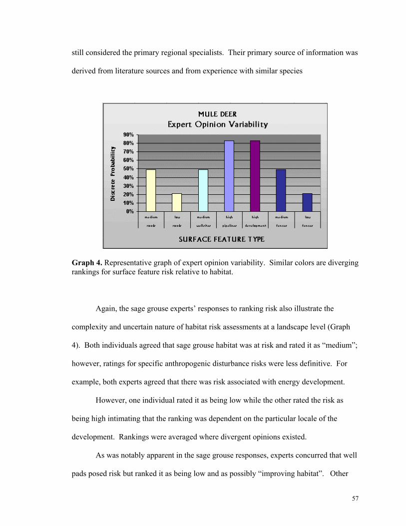
still considered the primary regional specialists. Their primary source of information was
derived from literature sources and from experience with similar species
Graph 4. Representative graph of expert opinion variability. Similar colors are diverging rankings for surface feature risk relative to habitat.
Again, the sage grouse experts’ responses to ranking risk also illustrate the
complexity and uncertain nature of habitat risk assessments at a landscape level (Graph
4). Both individuals agreed that sage grouse habitat was at risk and rated it as “medium”;
however, ratings for specific anthropogenic disturbance risks were less definitive. For
example, both experts agreed that there was risk associated with energy development.
However, one individual rated it as being low while the other rated the risk as
being high intimating that the ranking was dependent on the particular locale of the
development. Rankings were averaged where divergent opinions existed.
As was notably apparent in the sage grouse responses, experts concurred that well
pads posed risk but ranked it as being low and as possibly “improving habitat”. Other
57
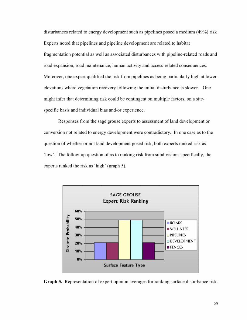
disturbances related to energy development such as pipelines posed a medium (49%) risk
Experts noted that pipelines and pipeline development are related to habitat
fragmentation potential as well as associated disturbances with pipeline-related roads and
road expansion, road maintenance, human activity and access-related consequences.
Moreover, one expert qualified the risk from pipelines as being particularly high at lower
elevations where vegetation recovery following the initial disturbance is slower. One
might infer that determining risk could be contingent on multiple factors, on a site-
specific basis and individual bias and/or experience.
Responses from the sage grouse experts to assessment of land development or
conversion not related to energy development were contradictory. In one case as to the
question of whether or not land development posed risk, both experts ranked risk as
‘low’. The follow-up question of as to ranking risk from subdivisions specifically, the
experts ranked the risk as ‘high’ (graph 5).
Graph 5. Representation of expert opinion averages for ranking surface disturbance risk.
58
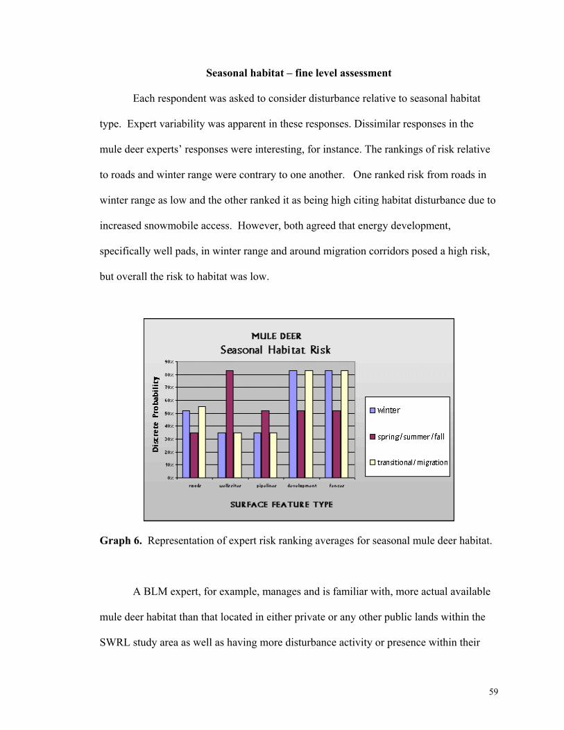
Seasonal habitat – fine level assessment
Each respondent was asked to consider disturbance relative to seasonal habitat
type. Expert variability was apparent in these responses. Dissimilar responses in the
mule deer experts’ responses were interesting, for instance. The rankings of risk relative
to roads and winter range were contrary to one another. One ranked risk from roads in
winter range as low and the other ranked it as being high citing habitat disturbance due to
increased snowmobile access. However, both agreed that energy development,
specifically well pads, in winter range and around migration corridors posed a high risk,
but overall the risk to habitat was low.
Graph 6. Representation of expert risk ranking averages for seasonal mule deer habitat.
A BLM expert, for example, manages and is familiar with, more actual available
mule deer habitat than that located in either private or any other public lands within the
SWRL study area as well as having more disturbance activity or presence within their
59
region. As compared to the responses of a Forest Service Range Conservationist, mule
deer habitat is limited to spring/summer and some fall ranges. As well, this particular
segment of National Forest has very limited oil, gas and land development and, similarly,
fewer roads and fences. Therefore, the Forest Service’s Range Conservationist responses
compared to that of the BLM’s Wildlife Biologist ranked risk lower with respect to roads
and fences, in particular.
At the conclusion of each interview, the respondents were asked from where their
knowledge of habitat risk was attributed. All six experts relied on personal observation
and experience in the region. Five of the six experts referred to literature although never
cited specific sources during the interview. All referred to their reliance on their peers for
sharing knowledge and information, from within the region and from within their
professional disciplines. And, finally, all often prefaced their rankings by stating that
risk from a particular disturbance was “site specific”; noting that landscape-level risk
determination for a single habitat was challenging.
The interview also included determining rankings related to more specific
disturbance types such as road density and road type. However, this information was
eliminated from the application within the BBN models for a number of reasons. Road
classification information was not available. Road density calculations, however, would
have been applicable and may be used in future research given more time.
BBN Models & CPT’s
The Belief Network models are intended to represent knowledge. Each node
represents discrete random variable values whereas the arcs represent the causal
60
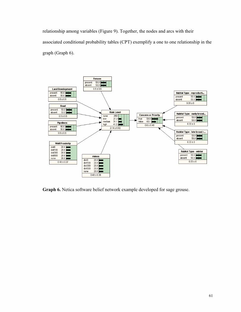
relationship among variables (Figure 9). Together, the nodes and arcs with their
associated conditional probability tables (CPT) exemplify a one to one relationship in the
graph (Graph 6).
Graph 6. Netica software belief network example developed for sage grouse.
61
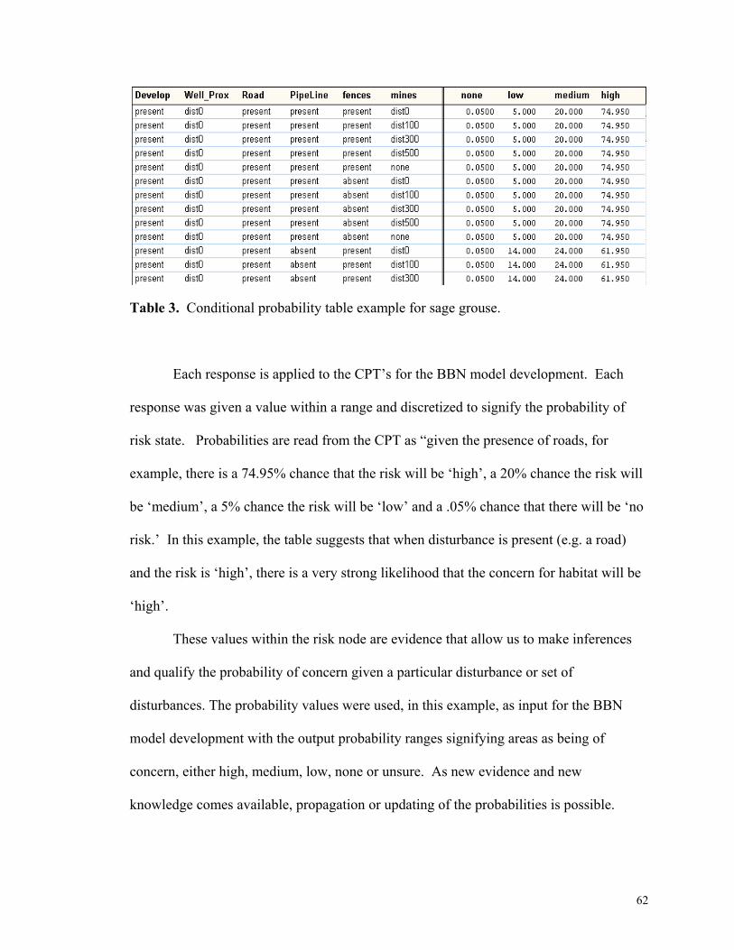
Table 3. Conditional probability table example for sage grouse.
Each response is applied to the CPT’s for the BBN model development. Each
response was given a value within a range and discretized to signify the probability of
risk state. Probabilities are read from the CPT as “given the presence of roads, for
example, there is a 74.95% chance that the risk will be ‘high’, a 20% chance the risk will
be ‘medium’, a 5% chance the risk will be ‘low’ and a .05% chance that there will be ‘no
risk.’ In this example, the table suggests that when disturbance is present (e.g. a road)
and the risk is ‘high’, there is a very strong likelihood that the concern for habitat will be
‘high’.
These values within the risk node are evidence that allow us to make inferences
and qualify the probability of concern given a particular disturbance or set of
disturbances. The probability values were used, in this example, as input for the BBN
model development with the output probability ranges signifying areas as being of
concern, either high, medium, low, none or unsure. As new evidence and new
knowledge comes available, propagation or updating of the probabilities is possible.
62
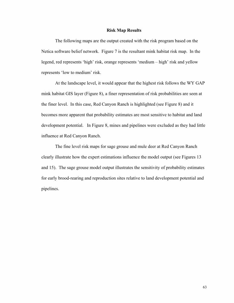
Risk Map Results
The following maps are the output created with the risk program based on the
Netica software belief network. Figure 7 is the resultant mink habitat risk map. In the
legend, red represents ‘high’ risk, orange represents ‘medium – high’ risk and yellow
represents ‘low to medium’ risk.
At the landscape level, it would appear that the highest risk follows the WY GAP
mink habitat GIS layer (Figure 8), a finer representation of risk probabilities are seen at
the finer level. In this case, Red Canyon Ranch is highlighted (see Figure 8) and it
becomes more apparent that probability estimates are most sensitive to habitat and land
development potential. In Figure 8, mines and pipelines were excluded as they had little
influence at Red Canyon Ranch.
The fine level risk maps for sage grouse and mule deer at Red Canyon Ranch
clearly illustrate how the expert estimations influence the model output (see Figures 13
and 15). The sage grouse model output illustrates the sensitivity of probability estimates
for early brood-rearing and reproduction sites relative to land development potential and
pipelines.
63
Figure 8. Risk map for mink habitat based on the Mink BBN model.
64
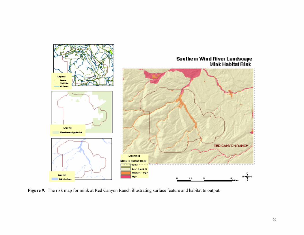
Figure 9. The risk map for mink at Red Canyon Ranch illustrating surface feature and habitat to output.
65

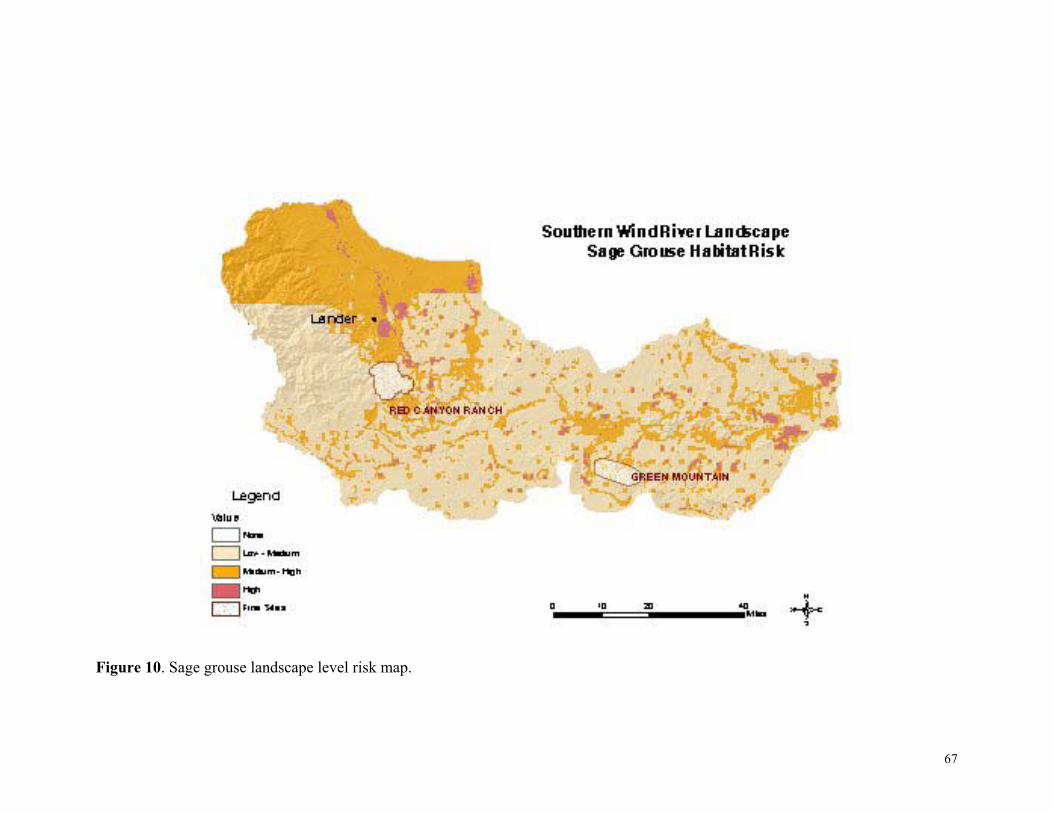
Figure 10. Sage grouse landscape level risk map.
67
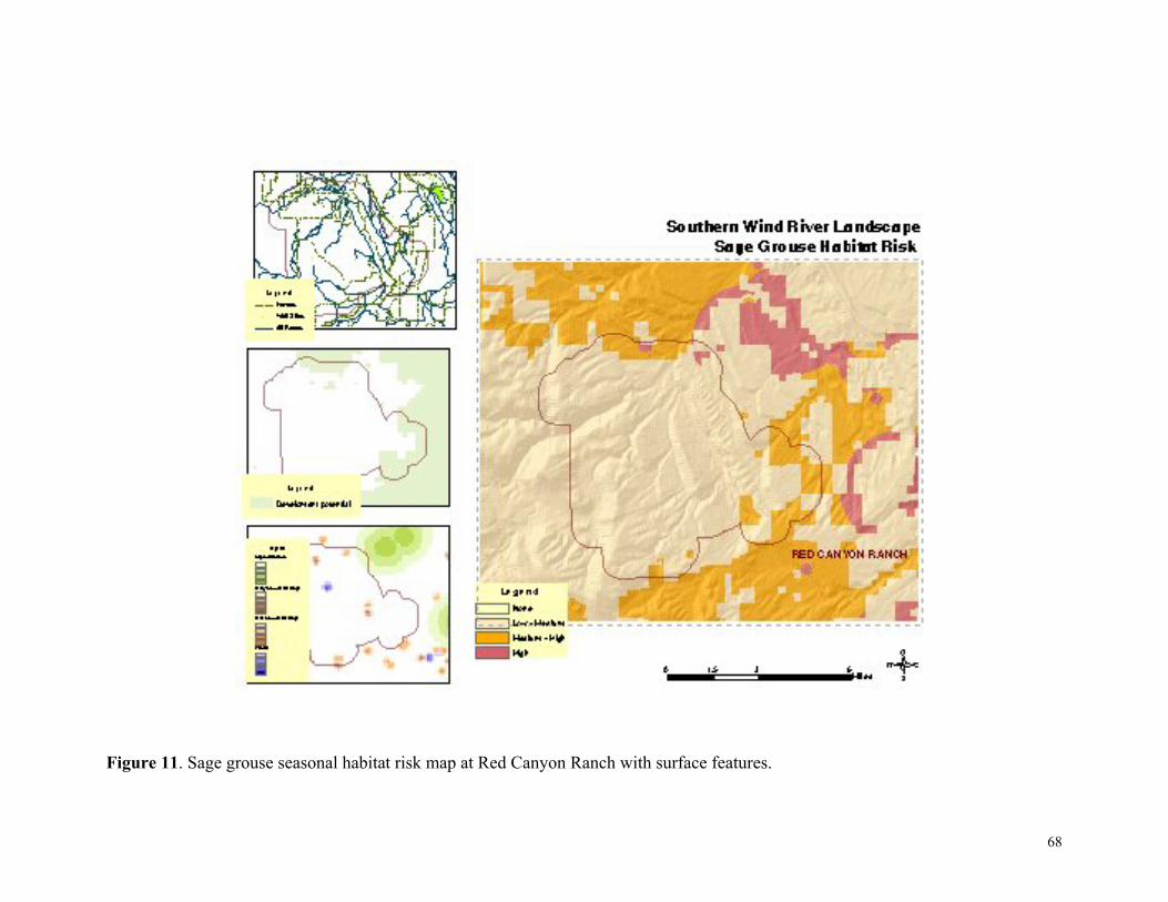
Figure 11. Sage grouse seasonal habitat risk map at Red Canyon Ranch with surface features.
68
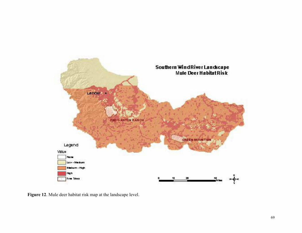
Figure 12. Mule deer habitat risk map at the landscape level.
69

Figure 13. Mule deer seasonal habitat risk map at Red Canyon Ranch with surface features.
70
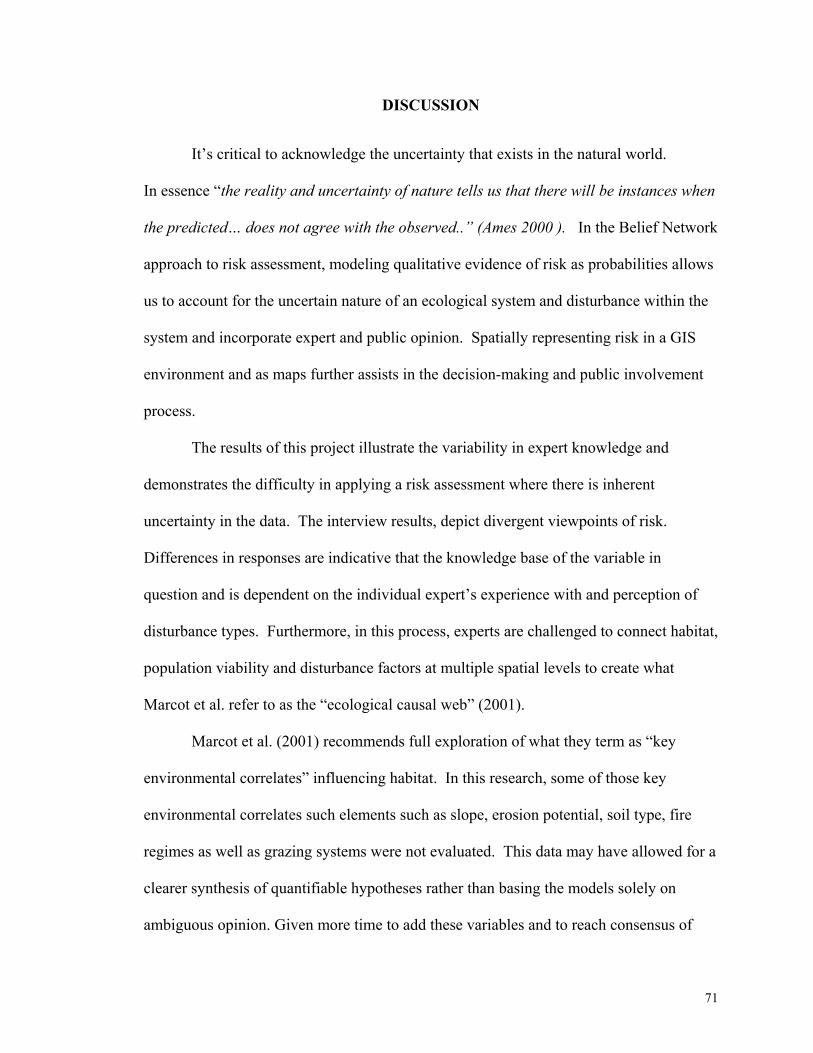
DISCUSSION It’s critical to acknowledge the uncertainty that exists in the natural world.
In essence “the reality and uncertainty of nature tells us that there will be instances when
the predicted… does not agree with the observed..” (Ames 2000 ). In the Belief Network
approach to risk assessment, modeling qualitative evidence of risk as probabilities allows
us to account for the uncertain nature of an ecological system and disturbance within the
system and incorporate expert and public opinion. Spatially representing risk in a GIS
environment and as maps further assists in the decision-making and public involvement
process.
The results of this project illustrate the variability in expert knowledge and
demonstrates the difficulty in applying a risk assessment where there is inherent
uncertainty in the data. The interview results, depict divergent viewpoints of risk.
Differences in responses are indicative that the knowledge base of the variable in
question and is dependent on the individual expert’s experience with and perception of
disturbance types. Furthermore, in this process, experts are challenged to connect habitat,
population viability and disturbance factors at multiple spatial levels to create what
Marcot et al. refer to as the “ecological causal web” (2001).
Marcot et al. (2001) recommends full exploration of what they term as “key
environmental correlates” influencing habitat. In this research, some of those key
environmental correlates such elements such as slope, erosion potential, soil type, fire
regimes as well as grazing systems were not evaluated. This data may have allowed for a
clearer synthesis of quantifiable hypotheses rather than basing the models solely on
ambiguous opinion. Given more time to add these variables and to reach consensus of
71
expert opinion would provide a more accurate picture of the physical processes across
that landscape contributing to habitat “risk”.
Accounting for response variability within the BBN exemplifies both the power
of the conditional probability tables used to establish risk rankings and the drawbacks and
error associated with applying the discrete variables based on the operator’s own
subjectivity.
Initially, expert responses were averaged. For instance, if one ranked risk as
‘high’ whereas the second expert ranked risk as being ‘medium’, one would expect that
averaging to establish a discrete ‘risk ranking’ was reasonable. However, in populating
the CPT’s of the model, that discrete value was not useful. The very basis of the BBN is
that there is some probability that there is either ‘no’, ‘low’, ‘medium’, or ‘high’ risk.
Therefore, in applying multiple expert opinions to the CPT, the operator is required to
determine, however subjectively, a discrete value for each ranking of probability.
Therefore, one would conclude that a failing in this approach is the estimation of applied
discrete variables.
Additionally, further meetings and follow-up with the professionals would have
been appropriate to determine if they concurred with the mapped results. Multiple
meetings would have also provided the research with true-to-life group decision-making
dynamics and ultimately consensus regarding risk. It also would have been appropriate
to include more individuals. Throughout the interviews, in fact, the experts
recommended that both retired nature resource professionals as well as lay people be
involved in the interviews.
72
Overall, the BBN and GIS program represented expert-based opinion of risk to
habitat relative to the available spatial data. However, factors not included such as road
type, road densities, active and non-active well sites and proximity to water course and
riparian systems may have allowed for clearer representation and determinations of risk.
Further adaptations to the Netica models such as ‘utility’ representing optimal
population numbers and ‘decision’ nodes representing land management options may
have provided a cost-benefit type analysis. And, finally, a cummulative assessment of all
disturbance relative to all habitats would have been interesting.
The BBN provides an opportunity for improving and adding to the decision-
making process; and providing quantifiable method for the determining either site
specific or landscape level risk aiding the planning process. Specifically, this approach
can be an effective tool in adaptive management strategies.
Model Validation Three validation opportunities may be applied to the Bayesian belief models
created in this project.
One may include an extensive ground-truthing process that entails multiple years
of observational studies of risk attributes at selected locales across the landscape. A blind
study, in this case, may be an appropriate validation method whereby field crews are not
aware of the current risk rankings. Their assessment may include a questionnaire
designed to capture a particular species’ presence and/or persistence at the selected sites.
Their independent, observational assessments will allow you to compare the computed
risks. A summary of these independent assessments and ranking the risks would allow
you to evaluate the estimates relative to the modeled results.
73

Two more immediate validation opportunities would include a second interview
with either the selected experts or different experts to assess the model and map results.
Again, interviewees would be asked a series of questions designed to ascertain whether
they agree or disagree with the modeled results at selected sites. The information
provided through a second interview would either verify or contradict the probabilities
weighting the model results and map output.
A final approach to validation used in this research was to utilize the built-in
Netica software sensitivity analyses function to determine which node/disturbance most
influenced the model results.
Sensitivity Analysis
Sensitivity analyses were conducted for each of the three models to explain the
variability in risk outcomes stemming from uncertainty about stressors and habitats.
According to Marcot et al. (2001), sensitivity is defined as the expected reduction in
variation of some query variable due to the conditional probability structure of the BBN
and the specific value of the parent nodes.
The sensitivity analysis is used to determine which nodes most influence the
outcome. Two sensitivity analyses were produced that reflect variance in the ‘Risk’
nodes and in the ‘Concern’ nodes. The risk node input are probabilities of risk based
solely on disturbance value. The concern node inputs are from both the risk node output
and the seasonal habitat node(s) (Appendix E).
The disturbances having the greatest influence on risk and concern levels are
development. For the sage grouse and mink, in particular, a manager or planner may
seek to focus their efforts on the effects of development with respect to these habitat
74

types. The sensitivity analyses can help identify priority areas and as new data is added,
the models can assist in determining areas of conservation, protection or rehabilitation
value, for example.
The Broader Implications
Adaptive management is a melding of acknowledgement of uncertainty with
sustainable land management (Lee 1986). It is a process in which there is:
1) a recognition of boundary management problems and constraints;
2) a representation of existing knowledge and one that models dynamism,
assumptions and predictions so continued learning is experienced;
3) representation and acknowledgement of uncertainty and alternative
hypotheses; and finally,
4) policy adaptation which allows for productivity and learning opportunities
(Walters 1986).
It is an iterative, decision-making process, based on present or a priori knowledge
(prior probability) which allows for the acceptance of new information in the evolution of
management objectives. In recent years, adaptive management strategies have been
applied to management of public lands and resources where public and private
cooperators have made attempts to manage for highly competitive resource demands
including fisheries, water and timber resources and for biodiversity.
In theory, adaptive management’s basic assumptions are probabilistic in nature.
In application, a Bayesian decision framework for the planning or management process
seeks to establish or quantify sets of all possible actions and outcomes. Adaptive
management methodology simply suggests that an individual or, in this case, a planner
75

will continue to revise his/her plans as new information becomes available. They can
adjust as ecological or societal “values” change. Humans will make decisions based on
current understanding of the world, but an adaptive management allows for knew
information to be accepted (Bergerud 1998).
76
LITERATURE CITED
Akçakaya, H.R. and L.R. Ginzburg. 1991. Ecological risk analysis for single and multiple populations. Species Conservation: A Population-Biological Approach. A. Seitz and V. Loeschcke (eds.) Birkhaeuser Verlag, Basel. Akçakaya, H. R. and M. G. Raphael. 1998. Assessing human impact despite uncertainty: viability of the northern spotted owl metapopulation in the northwestern USA. Biodiversity and Conservation 7:875-894. American Farmland Trust. [online] URL http://www.farmland.org/rocky_mountain/strategic_ranchlands3.htm Ames, D.P. 2002. Bayesian decision networks for watershed management. Ph.D. dissertation, Utah State University, Dept. of Civil and Environmental Engineering. Bailey, R. G.; Avers, P. E.; King, T.; McNab, W. H., eds. 1994. Ecoregions and Subregions of the United States (map). Washington, DC: USDA Forest Service. 1:7,500,000. with supplementary table of map unit descriptions, compiled and edited by W. H. McNab and R. G. Bailey. Bayesian Systems, Inc. [online] URL http://www.bayes.com/theorem.html Begon, M., J.L. Harper, and C.R. Townsend. 1996 Ecology: individuals, populations and communities. Blackwell Science, London. Berg, B. L. 2001. Qualitative Research Methods for the Social Sciences (4th ed.). Boston: Allyn & Bacon. Bergerud, W.A. and W.J. Reed. 1998. Bayesian statistical methods. Chapter 7. In V. Sit, and B. Taylor. (ed). 1998. Statistical methods for adaptive management studies. Res. Br., B.C. Min. For., Res. Br., Victoria, BC. Land Management Handbook 42. Bureau of Economic Analysis – Fremont Co. 2000. [online] URL http://www.fs.fed.us/r1/planning/econ/easy/library/cnty-wy-fremont/cnty-fremont.html Cairns, J., Jr. and P. V. McCormick. 1992. Developing an ecosystem-based capability for ecological risk assessments. The Environmental Professional 14:186-196. Charniak, E. 1991. Bayesian Networks Without Tears. AI Magazine, 12 4. Cohen, P. R. and Gruber, T. R. 1984. Reasoning about uncertainty: A knowledge representation approach. In Expert Systems: State of the Art Report, J. Fox (Ed.), Berkshire, England: Pergamon InfoTech Limited.
77
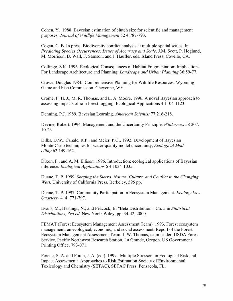
Cohen, Y. 1988. Bayesian estimation of clutch size for scientific and management purposes. Journal of Wildlife Management 52 4:787-793. Cogan, C. B. In press. Biodiversity conflict analysis at multiple spatial scales. In Predicting Species Occurrences: Issues of Accuracy and Scale. J.M. Scott, P. Heglund, M. Morrison, B. Wall, F. Samson, and J. Haufler, eds. Island Press, Covello, CA. Collinge, S.K. 1996. Ecological Consequences of Habitat Fragmentation: Implications For Landscape Architecture and Planning. Landscape and Urban Planning 36:59-77. Crowe, Douglas 1984. Comprehensive Planning for Wildlife Resources. Wyoming Game and Fish Commission. Cheyenne, WY. Crome, F. H. J., M. R. Thomas, and L. A. Moore. 1996. A novel Bayesian approach to assessing impacts of rain forest logging. Ecological Applications 4:1104-1123. Denning, P.J. 1989. Bayesian Learning. American Scientist 77:216-218. Devine, Robert. 1994. Management and the Uncertainty Principle. Wilderness 58 207: 10-23. Dilks, D.W., Canale, R.P., and Meier, P.G., 1992. Development of Bayesian Monte-Carlo techniques for water-quality model uncertainty, Ecological Mod- elling 62:149-162. Dixon, P., and A. M. Ellison. 1996. Introduction: ecological applications of Bayesian inference. Ecological Applications 6 4:1034-1035. Duane, T. P. 1999. Shaping the Sierra: Nature, Culture, and Conflict in the Changing West. University of California Press, Berkeley. 595 pp. Duane, T. P. 1997. Community Participation In Ecosystem Management. Ecology Law Quarterly 4 4: 771-797. Evans, M., Hastings, N.; and Peacock, B. "Beta Distribution." Ch. 5 in Statistical Distributions, 3rd ed. New York: Wiley, pp. 34-42, 2000. FEMAT (Forest Ecosystem Management Assessment Team). 1993. Forest ecosystem management: an ecological, economic, and social assessment. Report of the Forest Ecosystem Management Assessment Team, J. W. Thomas, team leader. USDA Forest Service, Pacific Northwest Research Station, La Grande, Oregon. US Government Printing Office. 793-071. Ferenc, S. A. and Foran, J. A. (ed.). 1999. Multiple Stressors in Ecological Risk and Impact Assessment: Approaches to Risk Estimation Society of Environmental Toxicology and Chemistry (SETAC), SETAC Press, Pensacola, FL.
78
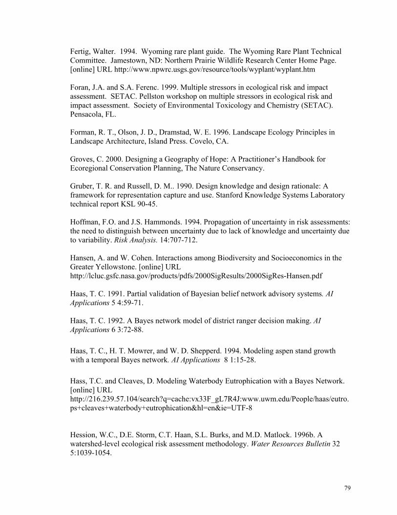
Fertig, Walter. 1994. Wyoming rare plant guide. The Wyoming Rare Plant Technical Committee. Jamestown, ND: Northern Prairie Wildlife Research Center Home Page. [online] URL http://www.npwrc.usgs.gov/resource/tools/wyplant/wyplant.htm Foran, J.A. and S.A. Ferenc. 1999. Multiple stressors in ecological risk and impact assessment. SETAC. Pellston workshop on multiple stressors in ecological risk and impact assessment. Society of Environmental Toxicology and Chemistry (SETAC). Pensacola, FL. Forman, R. T., Olson, J. D., Dramstad, W. E. 1996. Landscape Ecology Principles in Landscape Architecture, Island Press. Covelo, CA. Groves, C. 2000. Designing a Geography of Hope: A Practitioner’s Handbook for Ecoregional Conservation Planning, The Nature Conservancy. Gruber, T. R. and Russell, D. M.. 1990. Design knowledge and design rationale: A framework for representation capture and use. Stanford Knowledge Systems Laboratory technical report KSL 90-45. Hoffman, F.O. and J.S. Hammonds. 1994. Propagation of uncertainty in risk assessments: the need to distinguish between uncertainty due to lack of knowledge and uncertainty due to variability. Risk Analysis. 14:707-712. Hansen, A. and W. Cohen. Interactions among Biodiversity and Socioeconomics in the Greater Yellowstone. [online] URL http://lcluc.gsfc.nasa.gov/products/pdfs/2000SigResults/2000SigRes-Hansen.pdf Haas, T. C. 1991. Partial validation of Bayesian belief network advisory systems. AI Applications 5 4:59-71. Haas, T. C. 1992. A Bayes network model of district ranger decision making. AI Applications 6 3:72-88. Haas, T. C., H. T. Mowrer, and W. D. Shepperd. 1994. Modeling aspen stand growth with a temporal Bayes network. AI Applications 8 1:15-28. Hass, T.C. and Cleaves, D. Modeling Waterbody Eutrophication with a Bayes Network. [online] URL http://216.239.57.104/search?q=cache:vx33F_gL7R4J:www.uwm.edu/People/haas/eutro.ps+cleaves+waterbody+eutrophication&hl=en&ie=UTF-8 Hession, W.C., D.E. Storm, C.T. Haan, S.L. Burks, and M.D. Matlock. 1996b. A watershed-level ecological risk assessment methodology. Water Resources Bulletin 32 5:1039-1054.
79
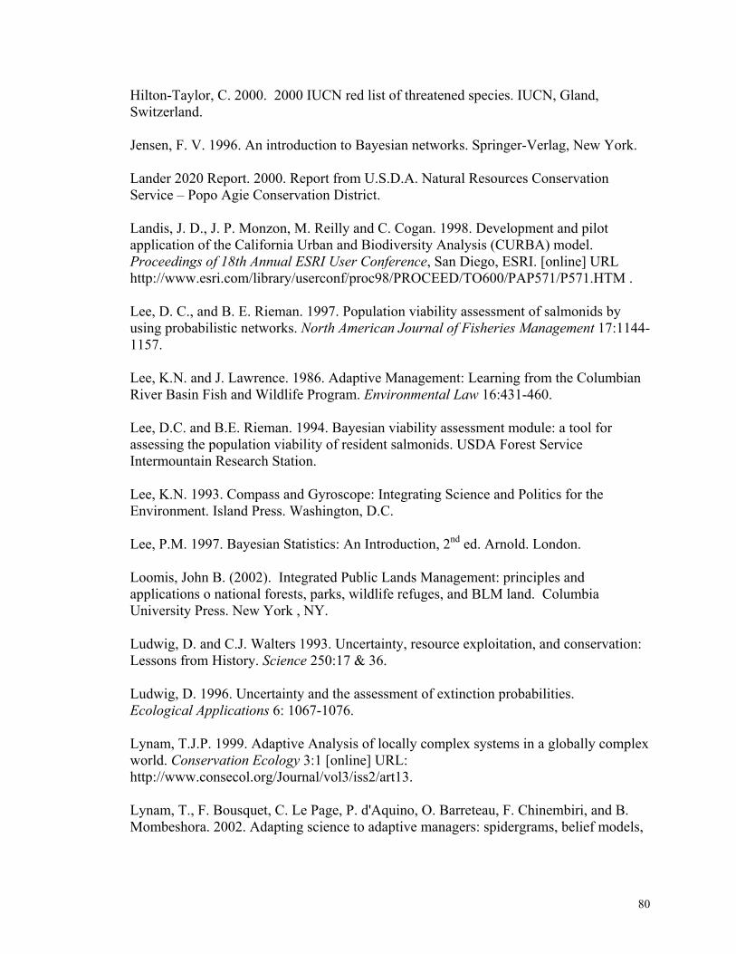
Hilton-Taylor, C. 2000. 2000 IUCN red list of threatened species. IUCN, Gland, Switzerland. Jensen, F. V. 1996. An introduction to Bayesian networks. Springer-Verlag, New York. Lander 2020 Report. 2000. Report from U.S.D.A. Natural Resources Conservation Service – Popo Agie Conservation District. Landis, J. D., J. P. Monzon, M. Reilly and C. Cogan. 1998. Development and pilot application of the California Urban and Biodiversity Analysis (CURBA) model. Proceedings of 18th Annual ESRI User Conference, San Diego, ESRI. [online] URL http://www.esri.com/library/userconf/proc98/PROCEED/TO600/PAP571/P571.HTM . Lee, D. C., and B. E. Rieman. 1997. Population viability assessment of salmonids by using probabilistic networks. North American Journal of Fisheries Management 17:1144-1157. Lee, K.N. and J. Lawrence. 1986. Adaptive Management: Learning from the Columbian River Basin Fish and Wildlife Program. Environmental Law 16:431-460. Lee, D.C. and B.E. Rieman. 1994. Bayesian viability assessment module: a tool for assessing the population viability of resident salmonids. USDA Forest Service Intermountain Research Station. Lee, K.N. 1993. Compass and Gyroscope: Integrating Science and Politics for the Environment. Island Press. Washington, D.C. Lee, P.M. 1997. Bayesian Statistics: An Introduction, 2nd ed. Arnold. London. Loomis, John B. (2002). Integrated Public Lands Management: principles and applications o national forests, parks, wildlife refuges, and BLM land. Columbia University Press. New York , NY. Ludwig, D. and C.J. Walters 1993. Uncertainty, resource exploitation, and conservation: Lessons from History. Science 250:17 & 36. Ludwig, D. 1996. Uncertainty and the assessment of extinction probabilities. Ecological Applications 6: 1067-1076. Lynam, T.J.P. 1999. Adaptive Analysis of locally complex systems in a globally complex world. Conservation Ecology 3:1 [online] URL: http://www.consecol.org/Journal/vol3/iss2/art13. Lynam, T., F. Bousquet, C. Le Page, P. d'Aquino, O. Barreteau, F. Chinembiri, and B. Mombeshora. 2002. Adapting science to adaptive managers: spidergrams, belief models,
80
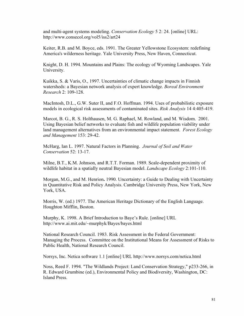
and multi-agent systems modeling. Conservation Ecology 5 2: 24. [online] URL: http://www.consecol.org/vol5/iss2/art24 Keiter, R.B. and M. Boyce, eds. 1991. The Greater Yellowstone Ecosystem: redefining America's wilderness heritage. Yale University Press, New Haven, Connecticut. Knight, D. H. 1994. Mountains and Plains: The ecology of Wyoming Landscapes. Yale University. Kuikka, S. & Varis, O., 1997. Uncertainties of climatic change impacts in Finnish watersheds: a Bayesian network analysis of expert knowledge. Boreal Environment Research 2: 109-128. MacIntosh, D.L., G.W. Suter II, and F.O. Hoffman. 1994. Uses of probabilistic exposure models in ecological risk assessments of contaminated sites. Risk Analysis 14 4:405-419. Marcot, B. G., R. S. Holthausen, M. G. Raphael, M. Rowland, and M. Wisdom. 2001. Using Bayesian belief networks to evaluate fish and wildlife population viability under land management alternatives from an environmental impact statement. Forest Ecology and Management 153: 29-42. McHarg, Ian L. 1997. Natural Factors in Planning. Journal of Soil and Water Conservation 52: 13-17. Milne, B.T., K.M. Johnson, and R.T.T. Forman. 1989. Scale-dependent proximity of wildlife habitat in a spatially neutral Bayesian model. Landscape Ecology 2:101-110. Morgan, M.G., and M. Henrion. 1990. Uncertainty: a Guide to Dealing with Uncertainty in Quantitative Risk and Policy Analysis. Cambridge University Press, New York, New York, USA. Morris, W. (ed.) 1977. The American Heritage Dictionary of the English Language. Houghton Mifflin, Boston. Murphy, K. 1998. A Brief Introduction to Baye’s Rule. [online] URL http://www.ai.mit.edu/~murphyk/Bayes/bayes.html National Research Council. 1983. Risk Assessment in the Federal Government: Managing the Process. Committee on the Institutional Means for Assessment of Risks to Public Health, National Research Council. Norsys, Inc. Netica software 1.1 [online] URL http://www.norsys.com/netica.html Noss, Reed F. 1994. "The Wildlands Project: Land Conservation Strategy," p233-266, in R. Edward Grumbine (ed.), Environmental Policy and Biodiversity, Washington, DC: Island Press.
81
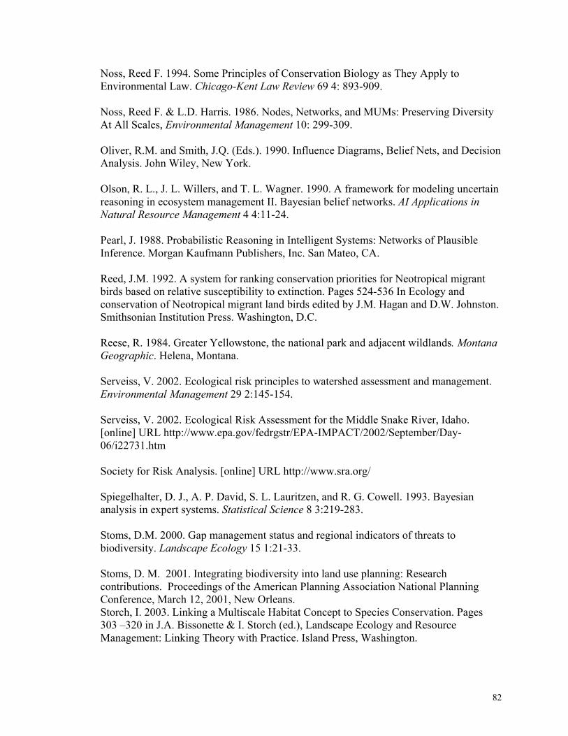
Noss, Reed F. 1994. Some Principles of Conservation Biology as They Apply to Environmental Law. Chicago-Kent Law Review 69 4: 893-909. Noss, Reed F. & L.D. Harris. 1986. Nodes, Networks, and MUMs: Preserving Diversity At All Scales, Environmental Management 10: 299-309. Oliver, R.M. and Smith, J.Q. (Eds.). 1990. Influence Diagrams, Belief Nets, and Decision Analysis. John Wiley, New York. Olson, R. L., J. L. Willers, and T. L. Wagner. 1990. A framework for modeling uncertain reasoning in ecosystem management II. Bayesian belief networks. AI Applications in Natural Resource Management 4 4:11-24. Pearl, J. 1988. Probabilistic Reasoning in Intelligent Systems: Networks of Plausible Inference. Morgan Kaufmann Publishers, Inc. San Mateo, CA. Reed, J.M. 1992. A system for ranking conservation priorities for Neotropical migrant birds based on relative susceptibility to extinction. Pages 524-536 In Ecology and conservation of Neotropical migrant land birds edited by J.M. Hagan and D.W. Johnston. Smithsonian Institution Press. Washington, D.C. Reese, R. 1984. Greater Yellowstone, the national park and adjacent wildlands. Montana Geographic. Helena, Montana. Serveiss, V. 2002. Ecological risk principles to watershed assessment and management. Environmental Management 29 2:145-154. Serveiss, V. 2002. Ecological Risk Assessment for the Middle Snake River, Idaho. [online] URL http://www.epa.gov/fedrgstr/EPA-IMPACT/2002/September/Day-06/i22731.htm Society for Risk Analysis. [online] URL http://www.sra.org/ Spiegelhalter, D. J., A. P. David, S. L. Lauritzen, and R. G. Cowell. 1993. Bayesian analysis in expert systems. Statistical Science 8 3:219-283. Stoms, D.M. 2000. Gap management status and regional indicators of threats to biodiversity. Landscape Ecology 15 1:21-33. Stoms, D. M. 2001. Integrating biodiversity into land use planning: Research contributions. Proceedings of the American Planning Association National Planning Conference, March 12, 2001, New Orleans. Storch, I. 2003. Linking a Multiscale Habitat Concept to Species Conservation. Pages 303 –320 in J.A. Bissonette & I. Storch (ed.), Landscape Ecology and Resource Management: Linking Theory with Practice. Island Press, Washington.
82
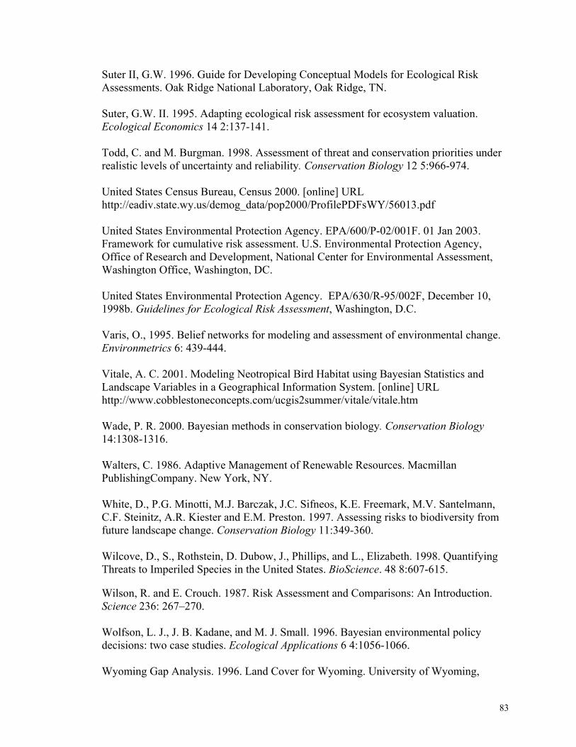
Suter II, G.W. 1996. Guide for Developing Conceptual Models for Ecological Risk Assessments. Oak Ridge National Laboratory, Oak Ridge, TN. Suter, G.W. II. 1995. Adapting ecological risk assessment for ecosystem valuation. Ecological Economics 14 2:137-141. Todd, C. and M. Burgman. 1998. Assessment of threat and conservation priorities under realistic levels of uncertainty and reliability. Conservation Biology 12 5:966-974. United States Census Bureau, Census 2000. [online] URL http://eadiv.state.wy.us/demog_data/pop2000/ProfilePDFsWY/56013.pdf United States Environmental Protection Agency. EPA/600/P-02/001F. 01 Jan 2003. Framework for cumulative risk assessment. U.S. Environmental Protection Agency, Office of Research and Development, National Center for Environmental Assessment, Washington Office, Washington, DC. United States Environmental Protection Agency. EPA/630/R-95/002F, December 10, 1998b. Guidelines for Ecological Risk Assessment, Washington, D.C. Varis, O., 1995. Belief networks for modeling and assessment of environmental change. Environmetrics 6: 439-444. Vitale, A. C. 2001. Modeling Neotropical Bird Habitat using Bayesian Statistics and Landscape Variables in a Geographical Information System. [online] URL http://www.cobblestoneconcepts.com/ucgis2summer/vitale/vitale.htm Wade, P. R. 2000. Bayesian methods in conservation biology. Conservation Biology 14:1308-1316. Walters, C. 1986. Adaptive Management of Renewable Resources. Macmillan PublishingCompany. New York, NY. White, D., P.G. Minotti, M.J. Barczak, J.C. Sifneos, K.E. Freemark, M.V. Santelmann, C.F. Steinitz, A.R. Kiester and E.M. Preston. 1997. Assessing risks to biodiversity from future landscape change. Conservation Biology 11:349-360. Wilcove, D., S., Rothstein, D. Dubow, J., Phillips, and L., Elizabeth. 1998. Quantifying Threats to Imperiled Species in the United States. BioScience. 48 8:607-615. Wilson, R. and E. Crouch. 1987. Risk Assessment and Comparisons: An Introduction. Science 236: 267–270. Wolfson, L. J., J. B. Kadane, and M. J. Small. 1996. Bayesian environmental policy decisions: two case studies. Ecological Applications 6 4:1056-1066. Wyoming Gap Analysis. 1996. Land Cover for Wyoming. University of Wyoming,
83

Spatial Data and Visualization Center Laramie, Wyoming. [online] URL http://www.sdvc.uwyo.edu/24k/landcov.html Wyoming Natural Diversity Database. Unpublished. Species of Special Concern Database, University of Wyoming, Laramie, Wyoming. Wyoming State Department of Administration and Information – Economic Analysis Division [online] URL http://eadiv.state.wy.us/i&e/i&e.asp
84

APPENDICES
Appendix A. Maps
85

Appendix A. Maps
86
Map 1. Southern Wind River Landscape Hydrologic Units – major, fourth order watersheds.
87
Map 2. Southern Wind River Landscape Surface Features – Roads.
88
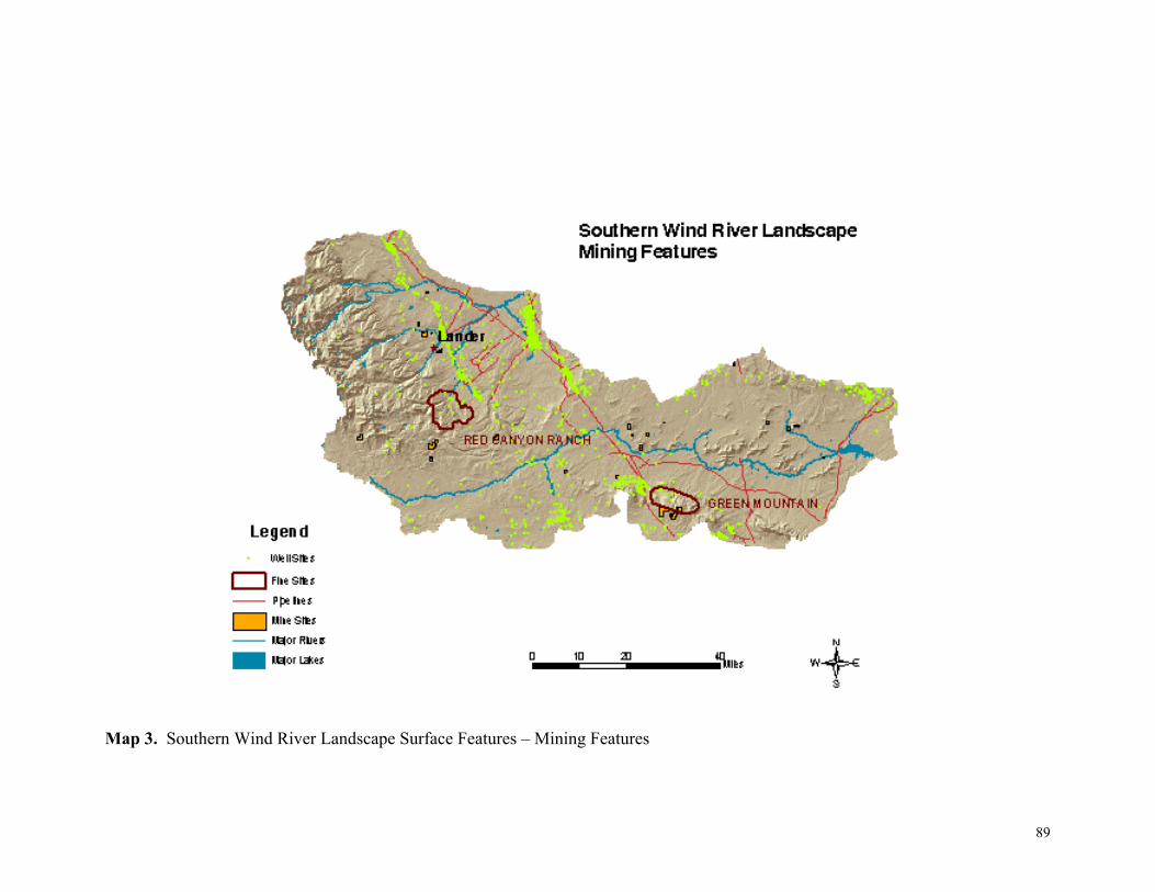
Map 3. Southern Wind River Landscape Surface Features – Mining Features
89
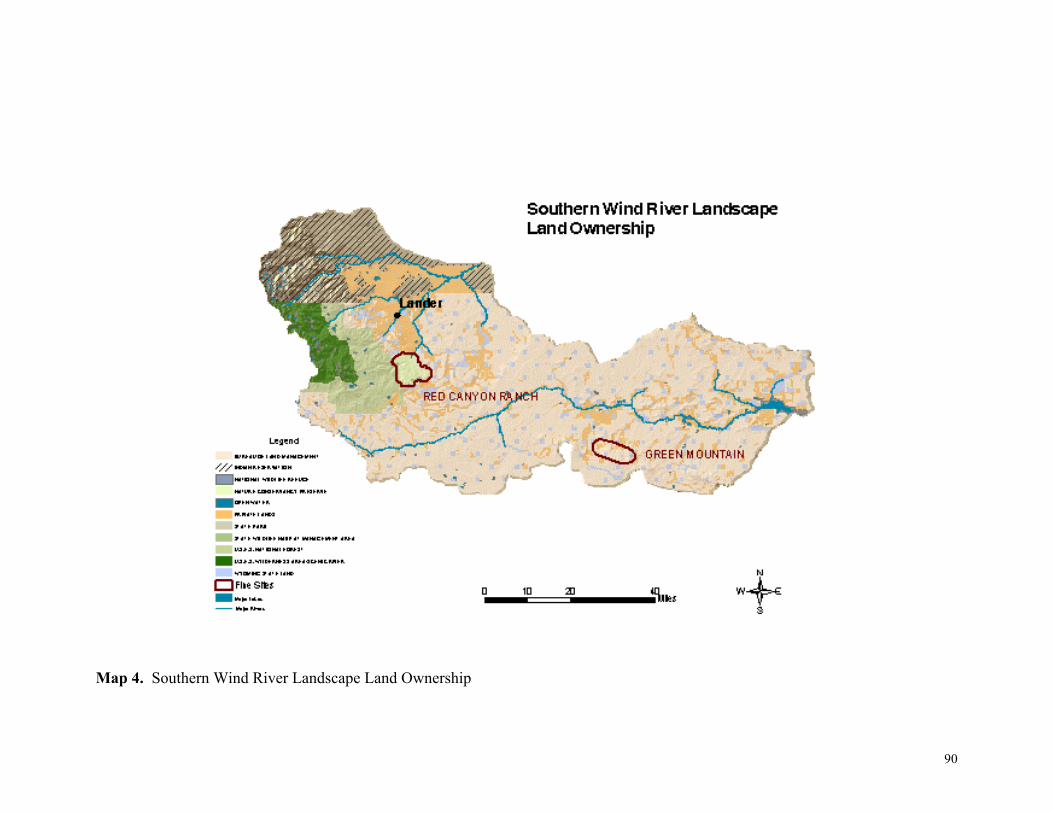
Map 4. Southern Wind River Landscape Land Ownership
90
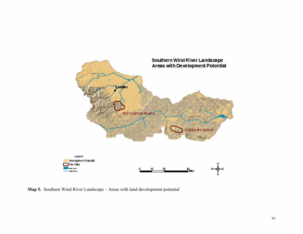
Map 5. Southern Wind River Landscape – Areas with land development potential
91
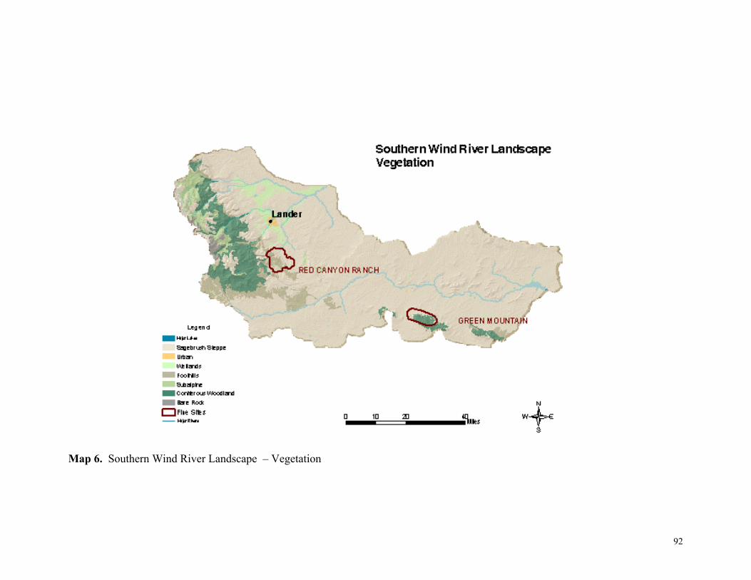
Map 6. Southern Wind River Landscape – Vegetation
92
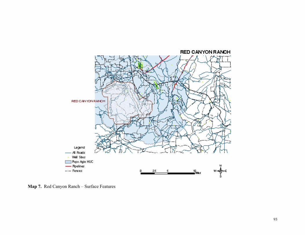
Map 7. Red Canyon Ranch – Surface Features
93

Map 8. Green Mountain – Surface Features
94
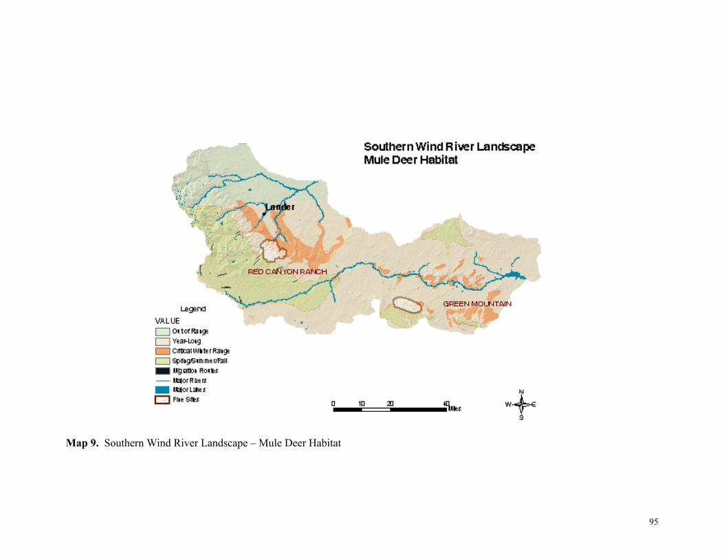
Map 9. Southern Wind River Landscape – Mule Deer Habitat
95
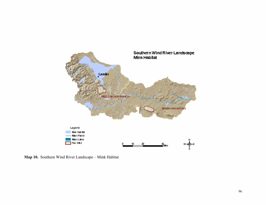
Map 10. Southern Wind River Landscape – Mink Habitat
96

Map 11. Southern Wind River Landscape – Sage Grouse Point Data
97
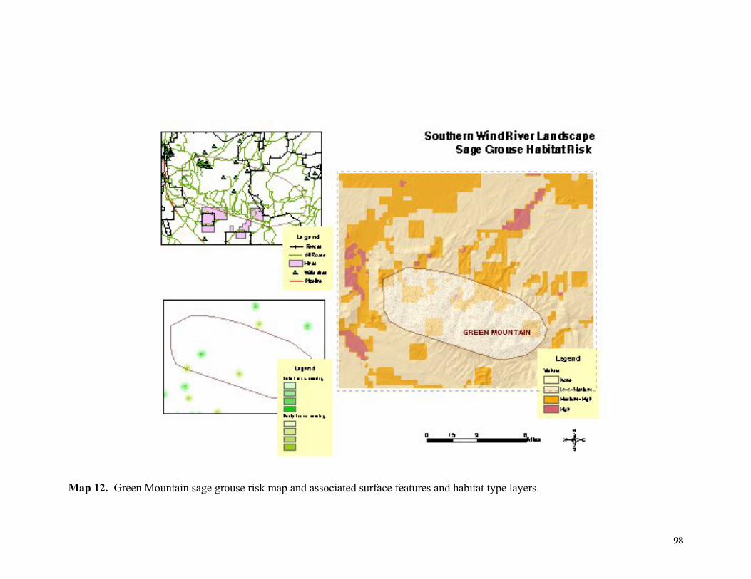
Map 12. Green Mountain sage grouse risk map and associated surface features and habitat type layers.
98
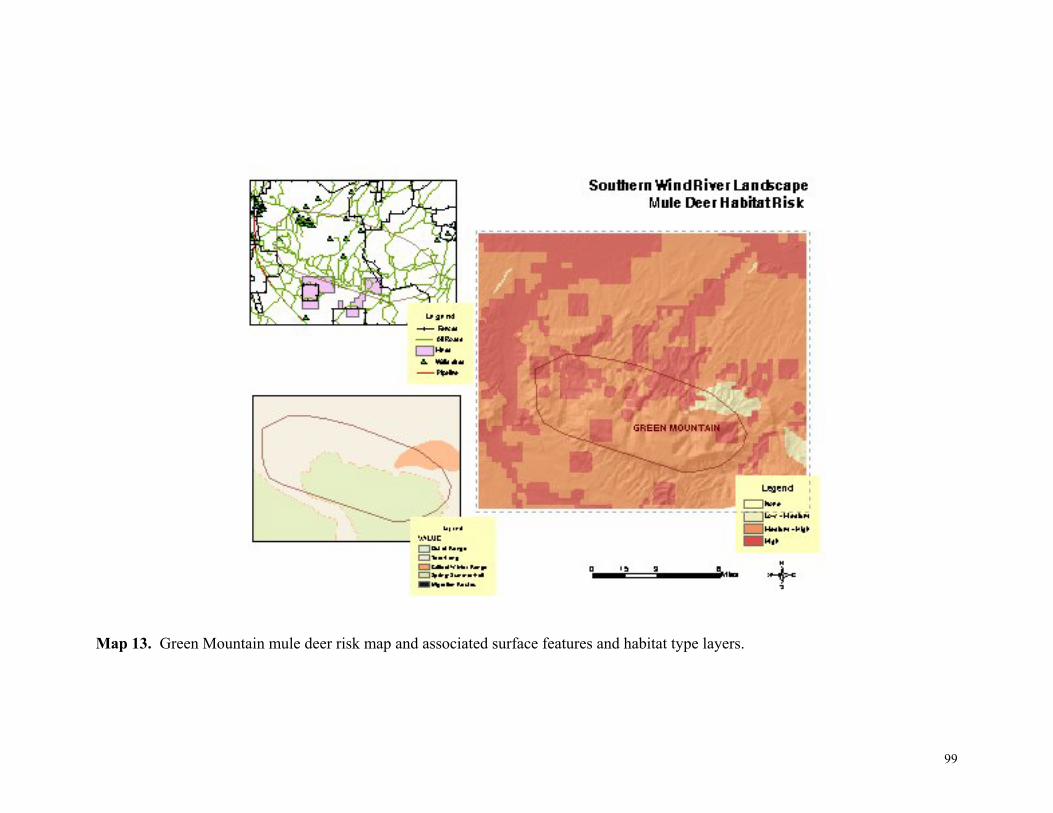
Map 13. Green Mountain mule deer risk map and associated surface features and habitat type layers.
99
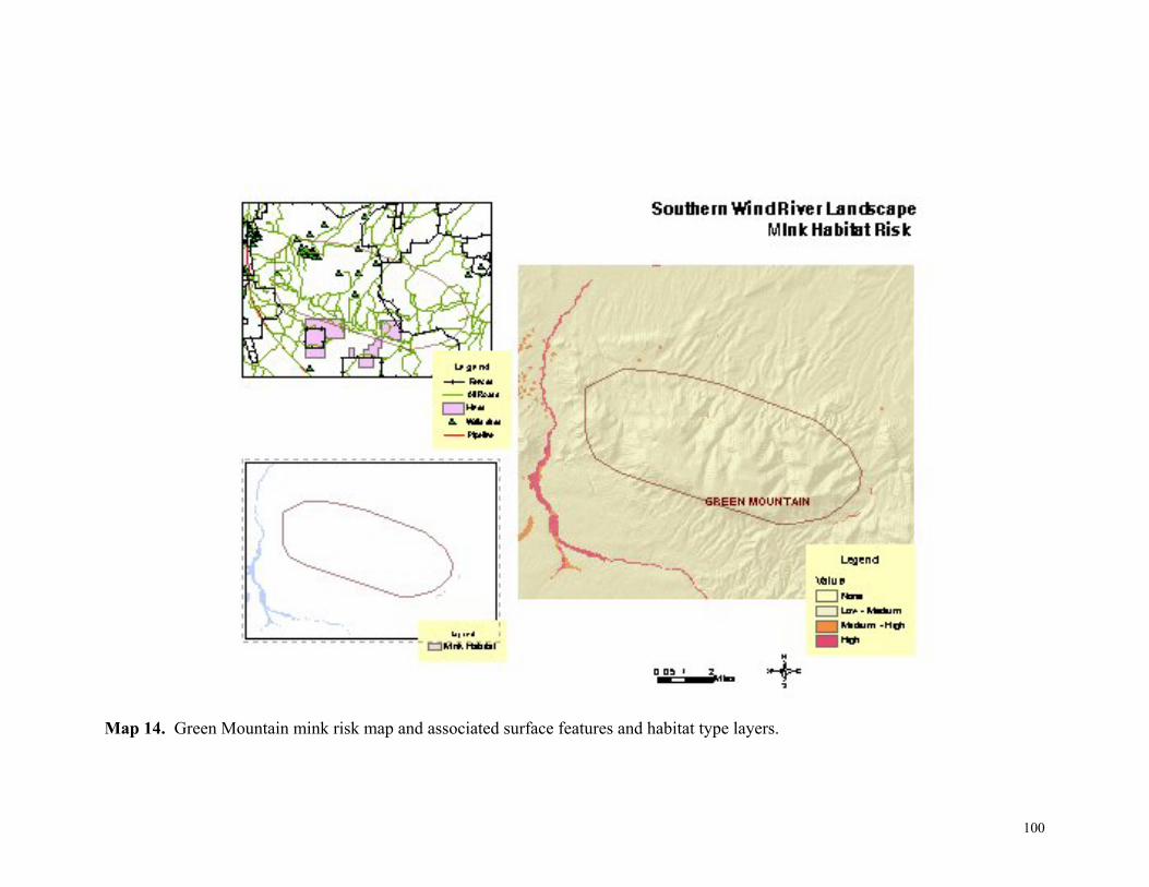
Map 14. Green Mountain mink risk map and associated surface features and habitat type layers.
100
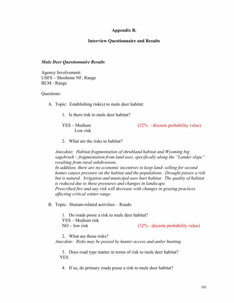
Appendix B.
Interview Questionnaire and Results
Mule Deer Questionnaire Results Agency Involvement: USFS – Shoshone NF, Range BLM - Range Questions:
A. Topic: Establishing risk(s) to mule deer habitat:
1. Is there risk to mule deer habitat? YES – Medium (32% - discrete probability value)
Low risk 2. What are the risks to habitat?
Anecdote: Habitat fragmentation of shrubland habitat and Wyoming big sagebrush – fragmentation from land uses, specifically along the “Lander slope” resulting from rural subdivisions. In addition, there are no economic incentives to keep land- selling for second homes causes pressure on the habitat and the populations. Drought posses a risk but is natural. Irrigation and municipal uses hurt habitat. The quality of habitat is reduced due to these pressures and changes in landscape. Prescribed fire and any risk will decrease with changes in grazing practices affecting critical winter range.
B. Topic: Human-related activities – Roads:
1. Do roads posse a risk to mule deer habitat? YES – Medium risk NO – low risk (32% - discrete probability value) 2. What are those risks?
Anecdote: Risks may be possed by hunter access and antler hunting
3. Does road type matter in terms of risk to mule deer habitat? YES
4. If so, do primary roads posse a risk to mule deer habitat?
101
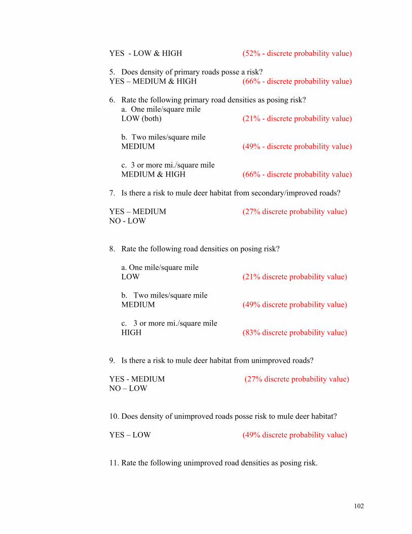
YES - LOW & HIGH (52% - discrete probability value) 5. Does density of primary roads posse a risk? YES – MEDIUM & HIGH (66% - discrete probability value) 6. Rate the following primary road densities as posing risk?
a. One mile/square mile LOW (both) (21% - discrete probability value)
b. Two miles/square mile MEDIUM (49% - discrete probability value)
c. 3 or more mi./square mile MEDIUM & HIGH (66% - discrete probability value) 7. Is there a risk to mule deer habitat from secondary/improved roads? YES – MEDIUM (27% discrete probability value) NO - LOW 8. Rate the following road densities on posing risk?
a. One mile/square mile LOW (21% discrete probability value)
b. Two miles/square mile MEDIUM (49% discrete probability value)
c. 3 or more mi./square mile HIGH (83% discrete probability value)
9. Is there a risk to mule deer habitat from unimproved roads?
YES - MEDIUM (27% discrete probability value) NO – LOW 10. Does density of unimproved roads posse risk to mule deer habitat?
YES – LOW (49% discrete probability value) 11. Rate the following unimproved road densities as posing risk.
102

a. One mile/square mile LOW (21% discrete probability value)
b. Two miles/square mile MEDIUM (49% discrete probability value)
c. 3 or more mi./square mile HIGH (83% discrete probability value)
12. Do roads posse risk to seasonal mule deer habitat?
YES – MEDIUM (44% discrete probability value) NOT SURE 13. Rate the risk to each seasonal habitat type from roads.
a. Winter Range HIGH & LOW (52% discrete probability value)
b. Summer MEDIUM & LOW (35% discrete probability value)
c. Migration LOW & MEDIUM (35% discrete probability value)
d. Yearlong (21% discrete probability value)
LOW
C. Topic: Other Surface Features: Energy Development 1. Does energy development posse risk to mule deer habitat?
YES - LOW (16% discrete probability value)
Anecdote: site specific in winter range; higher risk in winter range
2. What are the risks posed by energy development to mule deer habitat?
Fences
103

3. Rate the risk to each seasonal habitat type from energy development.
a. Winter MEDIUM (49% discrete probability value)
b. Summer LOW (21% discrete probability value)
c. Migration LOW & MEDIUM (35% discrete probability value) d. Yearlong LOW & MEDIUM (35% discrete probability value)
4. Do well pads posse a risk to mule deer habitat?
YES 5. At what proximity to mule deer habitat do well pads posse a risk?
a. 0 – 100m HIGH (83% discrete probability value) b. 100 – 300m LOW & MEDIUM (35% discrete probability value) c. 300 – 500m LOW (both) (21% discrete probability value)
6. Rate the risk to each seasonal habitat type from well pads.
a. Winter Range HIGH & LOW (52% discrete probability value)
b. Summer MEDIUM & LOW (35% discrete probability value) c. Migration HIGH & MEDIUM (66% discrete probability value) d. Yearlong LOW & MEDIUM (35% discrete probability value)
104

7. Do pipelines posse a risk to mule deer habitat?
YES – HIGH (83% discrete probability value)
Anecdote: dependent on time – within 3 – 5 years risks are higher and improves after 5 yrs.
8. At what proximity to mule deer habitat pipelines posse a risk?
a. 0 – 100m LOW (21% discrete probability value)
b. 100 – 300m LOW (21% discrete probability value)
c. 300 – 500m LOW (21% discrete probability value)
9. Rate the risk to each seasonal habitat type from pipelines.
a.Winter Range LOW (21% discrete probability value)
b. Summer MEDIUM & LOW (35% discrete probability value)
c. Migration LOW & MEDIUM (35% discrete probability value) d. Yearlong LOW & MEDIUM (35% discrete probability value)
D. Topic: Other Surface Features: Land Development
1. Fences posse a risk to mule deer habitat?
YES – MEDIUM (35% discrete probability value) NO – LOW
2. Does land conversion posse a risk to mule deer habitat?
105
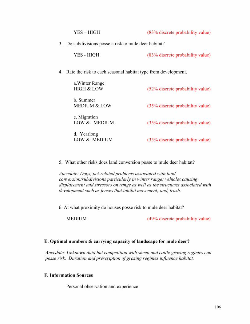
YES – HIGH (83% discrete probability value)
3. Do subdivisions posse a risk to mule deer habitat?
YES - HIGH (83% discrete probability value)
4. Rate the risk to each seasonal habitat type from development.
a.Winter Range HIGH & LOW (52% discrete probability value)
b. Summer MEDIUM & LOW (35% discrete probability value) c. Migration LOW & MEDIUM (35% discrete probability value) d. Yearlong LOW & MEDIUM (35% discrete probability value)
5. What other risks does land conversion posse to mule deer habitat?
Anecdote: Dogs, pet-related problems associated with land conversion/subdivisions particularly in winter range; vehicles causing displacement and stressors on range as well as the structures associated with development such as fences that inhibit movement; and, trash. 6. At what proximity do houses posse risk to mule deer habitat?
MEDIUM (49% discrete probability value)
E. Optimal numbers & carrying capacity of landscape for mule deer?
Anecdote: Unknown data but competition with sheep and cattle grazing regimes can posse risk. Duration and prescription of grazing regimes influence habitat.
F. Information Sources
Personal observation and experience
106
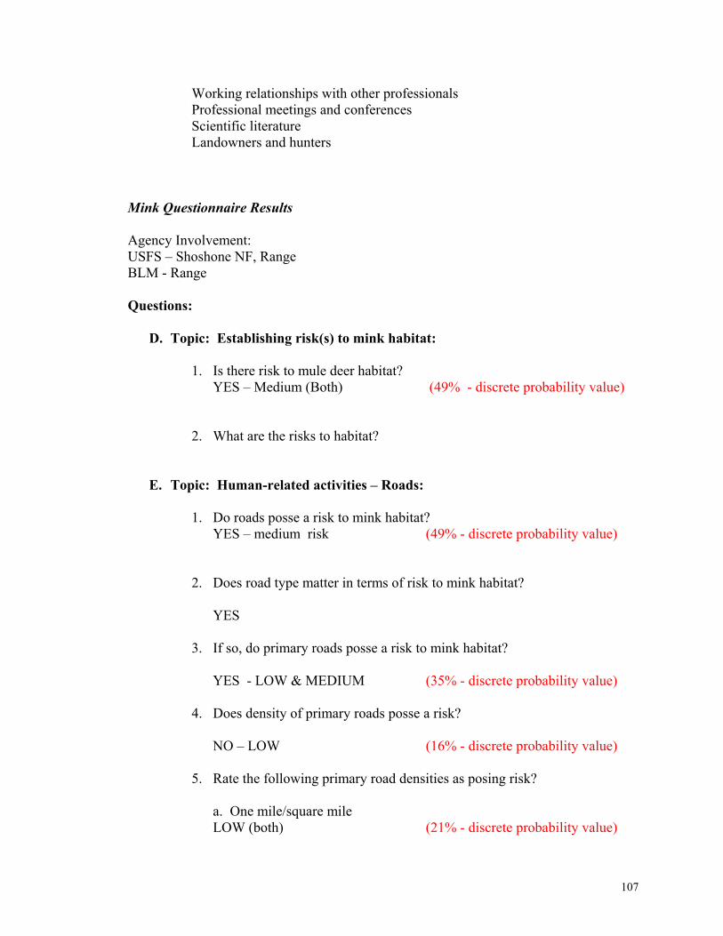
Working relationships with other professionals Professional meetings and conferences Scientific literature Landowners and hunters
Personal Antler hunting
Mink Questionnaire Results Agency Involvement: USFS – Shoshone NF, Range BLM - Range Questions:
D. Topic: Establishing risk(s) to mink habitat:
1. Is there risk to mule deer habitat? YES – Medium (Both) (49% - discrete probability value)
2. What are the risks to habitat?
E. Topic: Human-related activities – Roads:
1. Do roads posse a risk to mink habitat? YES – medium risk (49% - discrete probability value)
2. Does road type matter in terms of risk to mink habitat?
YES 3. If so, do primary roads posse a risk to mink habitat?
YES - LOW & MEDIUM (35% - discrete probability value)
4. Does density of primary roads posse a risk?
NO – LOW (16% - discrete probability value) 5. Rate the following primary road densities as posing risk?
a. One mile/square mile LOW (both) (21% - discrete probability value)
107
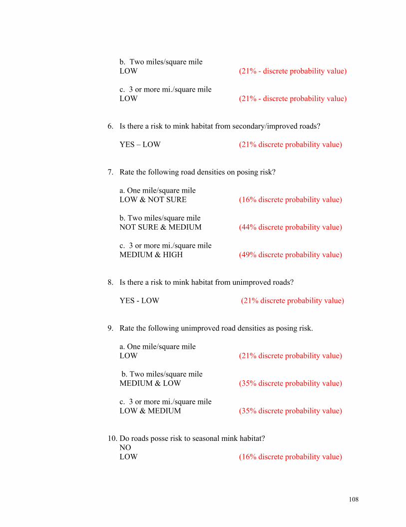
b. Two miles/square mile
LOW (21% - discrete probability value)
c. 3 or more mi./square mile LOW (21% - discrete probability value) 6. Is there a risk to mink habitat from secondary/improved roads?
YES – LOW (21% discrete probability value)
7. Rate the following road densities on posing risk?
a. One mile/square mile LOW & NOT SURE (16% discrete probability value)
b. Two miles/square mile NOT SURE & MEDIUM (44% discrete probability value)
c. 3 or more mi./square mile MEDIUM & HIGH (49% discrete probability value)
8. Is there a risk to mink habitat from unimproved roads?
YES - LOW (21% discrete probability value)
9. Rate the following unimproved road densities as posing risk.
a. One mile/square mile LOW (21% discrete probability value)
b. Two miles/square mile MEDIUM & LOW (35% discrete probability value)
c. 3 or more mi./square mile LOW & MEDIUM (35% discrete probability value)
10. Do roads posse risk to seasonal mink habitat?
NO LOW (16% discrete probability value)
108
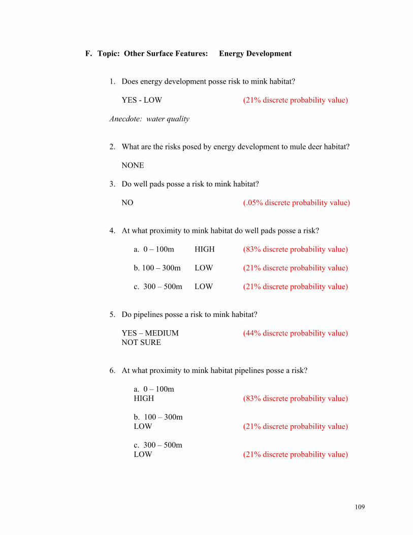
F. Topic: Other Surface Features: Energy Development
1. Does energy development posse risk to mink habitat?
YES - LOW (21% discrete probability value)
Anecdote: water quality
2. What are the risks posed by energy development to mule deer habitat?
NONE
3. Do well pads posse a risk to mink habitat?
NO (.05% discrete probability value) 4. At what proximity to mink habitat do well pads posse a risk?
a. 0 – 100m HIGH (83% discrete probability value)
b. 100 – 300m LOW (21% discrete probability value)
c. 300 – 500m LOW (21% discrete probability value)
5. Do pipelines posse a risk to mink habitat?
YES – MEDIUM (44% discrete probability value) NOT SURE
6. At what proximity to mink habitat pipelines posse a risk?
a. 0 – 100m HIGH (83% discrete probability value)
b. 100 – 300m LOW (21% discrete probability value)
c. 300 – 500m LOW (21% discrete probability value)
109

D. Topic: Land Development
1. Do fences posse a risk to mink habitat?
NO (.05 % discrete probability value)
2. Does land conversion posse a risk to mink habitat?
YES – MEDIUM (49% discrete probability value)
3. Do subdivisions posse a risk to mink habitat?
YES - MEDIUM (49% discrete probability value)
4. What other risks does land conversion posse to mink habitat?
Anecdote: Dogs, pet-related problems associated with land conversion or subdivisions particularly roads causing loss of habitat, spraying lands with pesticides.
5. At what proximity do houses posse risk to mink habitat? Anecdote: The species is adaptive to human activities; but shy and will avoid audible and visual disturbances
E. Optimal numbers & carrying capacity of landscape for mink? Unknown Data F. Information Sources
Personal observation and experience Working relationships with other professionals Professional meetings and conferences Scientific literature Landowners and hunters
110
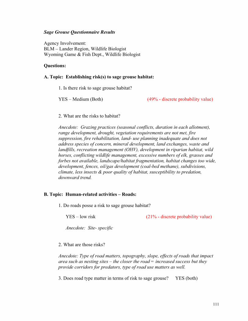
Sage Grouse Questionnaire Results Agency Involvement: BLM – Lander Region, Wildlife Biologist Wyoming Game & Fish Dept., Wildlife Biologist Questions: A. Topic: Establishing risk(s) to sage grouse habitat:
1. Is there risk to sage grouse habitat? YES – Medium (Both) (49% - discrete probability value)
2. What are the risks to habitat?
Anecdote: Grazing practices (seasonal conflicts, duration in each allotment), range development, drought, vegetation requirements are not met, fire suppression, fire rehabilitation, land- use planning inadequate and does not address species of concern, mineral development, land exchanges, waste and landfills, recreation management (OHV), development in riparian habitat, wild horses, conflicting wildlife management, excessive numbers of elk, grasses and forbes not available, landscape/habitat fragmentation, habitat changes too wide, development, fences, oil/gas development (coal-bed methane), subdivisions, climate, less insects & poor quality of habitat, susceptibility to predation, downward trend.
B. Topic: Human-related activities – Roads:
1. Do roads posse a risk to sage grouse habitat?
YES – low risk (21% - discrete probability value) Anecdote: Site- specific
2. What are those risks?
Anecdote: Type of road matters, topography, slope, effects of roads that impact area such as nesting sites – the closer the road = increased success but they provide corridors for predators, type of road use matters as well.
3. Does road type matter in terms of risk to sage grouse? YES (both)
111
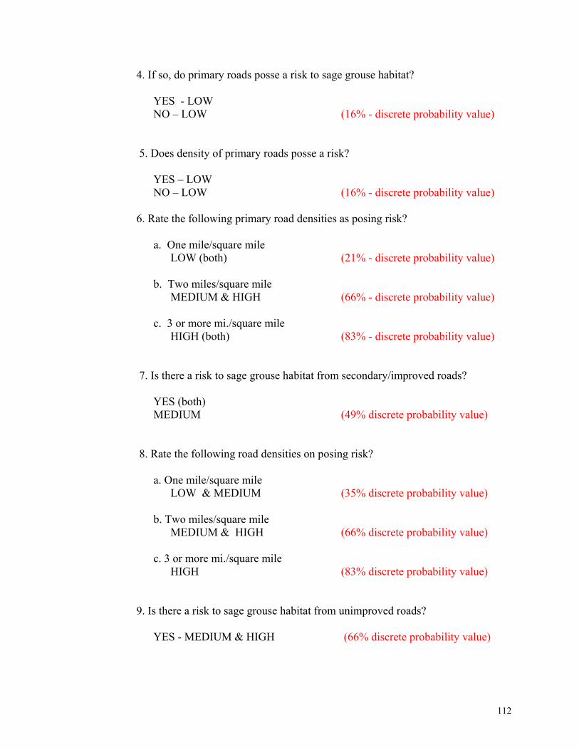
4. If so, do primary roads posse a risk to sage grouse habitat?
YES - LOW NO – LOW (16% - discrete probability value)
5. Does density of primary roads posse a risk? YES – LOW NO – LOW (16% - discrete probability value)
6. Rate the following primary road densities as posing risk? a. One mile/square mile LOW (both) (21% - discrete probability value) b. Two miles/square mile MEDIUM & HIGH (66% - discrete probability value) c. 3 or more mi./square mile HIGH (both) (83% - discrete probability value)
7. Is there a risk to sage grouse habitat from secondary/improved roads?
YES (both) MEDIUM (49% discrete probability value)
8. Rate the following road densities on posing risk? a. One mile/square mile
LOW & MEDIUM (35% discrete probability value) b. Two miles/square mile
MEDIUM & HIGH (66% discrete probability value) c. 3 or more mi./square mile
HIGH (83% discrete probability value)
9. Is there a risk to sage grouse habitat from unimproved roads?
YES - MEDIUM & HIGH (66% discrete probability value)
112
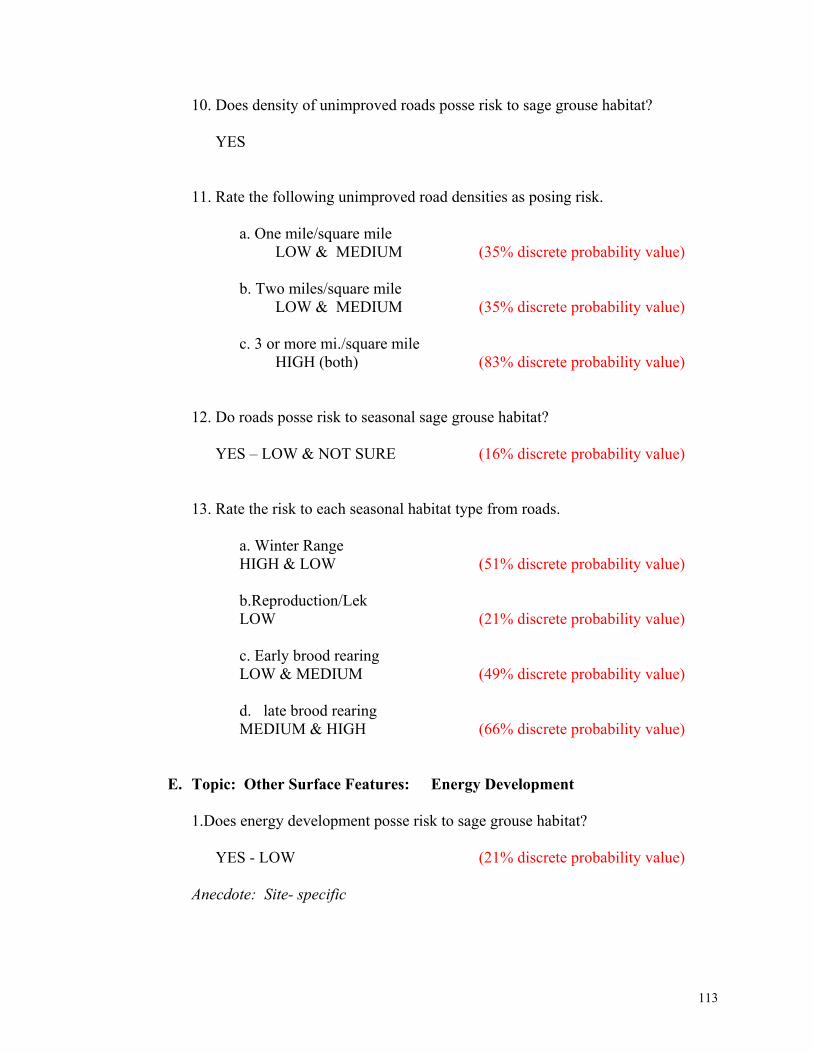
10. Does density of unimproved roads posse risk to sage grouse habitat?
YES
11. Rate the following unimproved road densities as posing risk.
a. One mile/square mile LOW & MEDIUM (35% discrete probability value)
b. Two miles/square mile LOW & MEDIUM (35% discrete probability value)
c. 3 or more mi./square mile HIGH (both) (83% discrete probability value)
12. Do roads posse risk to seasonal sage grouse habitat?
YES – LOW & NOT SURE (16% discrete probability value)
13. Rate the risk to each seasonal habitat type from roads.
a. Winter Range HIGH & LOW (51% discrete probability value)
b.Reproduction/Lek LOW (21% discrete probability value)
c. Early brood rearing LOW & MEDIUM (49% discrete probability value)
d. late brood rearing MEDIUM & HIGH (66% discrete probability value)
E. Topic: Other Surface Features: Energy Development
1.Does energy development posse risk to sage grouse habitat?
YES - LOW (21% discrete probability value)
Anecdote: Site- specific
113

2. What are the risks posed by energy development to sage grouse habitat? Anecdote: Density of development. Risk is attributed to fragmentation of habitat from roads, noise related to wells, compressor plants, road traffic = lek abandonment and other human uses such as overall disturbance, habitat loss from development construction and facilities.
4 wells/section and the number of roads = 2.5 mile/one square mile MEDIUM RISK (49% discrete probability value) 16 wells/section and the number of roads = 2.5 mile/square mile of HIGH RISK (83% discrete probability value)
4. Rate the risk to each seasonal habitat type from energy development.
a. Winter Range YES-LOW (21% discrete probability value)
b. Reproduction YES-MEDIUM (49% discrete probability value)
c. EBR
YES MEDIUM (49% discrete probability value)
d. LBR LOW (21% discrete probability value)
5. Do well pads posse a risk to sage grouse habitat?
YES - LOW (21% discrete probability value) Anecdote: may improve habitat
6. At what proximity to sage grouse habitat do well pads posse a risk?
a. 0 – 100m HIGH (83% discrete probability value)
b. 100 – 300m LOW & MEDIUM (35% discrete probability value)
114

c. 300 – 500m LOW (both) (21% discrete probability value)
7. Rate the risk to each seasonal habitat type from well pads.
a. Winter Range YES LOW (21% discrete probability value)
b. Reproduction YES HIGH (both) (83% discrete probability value)
c. EBR
YES MEDIUM & HIGH (66% discrete probability value)
d. LBR (35% discrete probability value) LOW & MEDIUM
8. Do pipelines posse a risk to sage grouse habitat?
YES – MEDIUM (49% discrete probability value)
Anecdote: risk from fragmentation, pipelines become predator travel corridors, roads associated with pipelines, and the physical reduction of high quality habitat = loss of habitat particularly in lower elevations.
9. At what proximity to sage grouse habitat pipelines posse a risk?
a. 0 – 100m HIGH (83% discrete probability value)
b. 100 – 300m MEDIUM & LOW (35% discrete probability value)
c. 300 – 500m LOW (21% discrete probability value)
10. Rate the risk to each seasonal habitat type from pipelines.
a. Winter Range NO & LOW (13% discrete probability value)
115
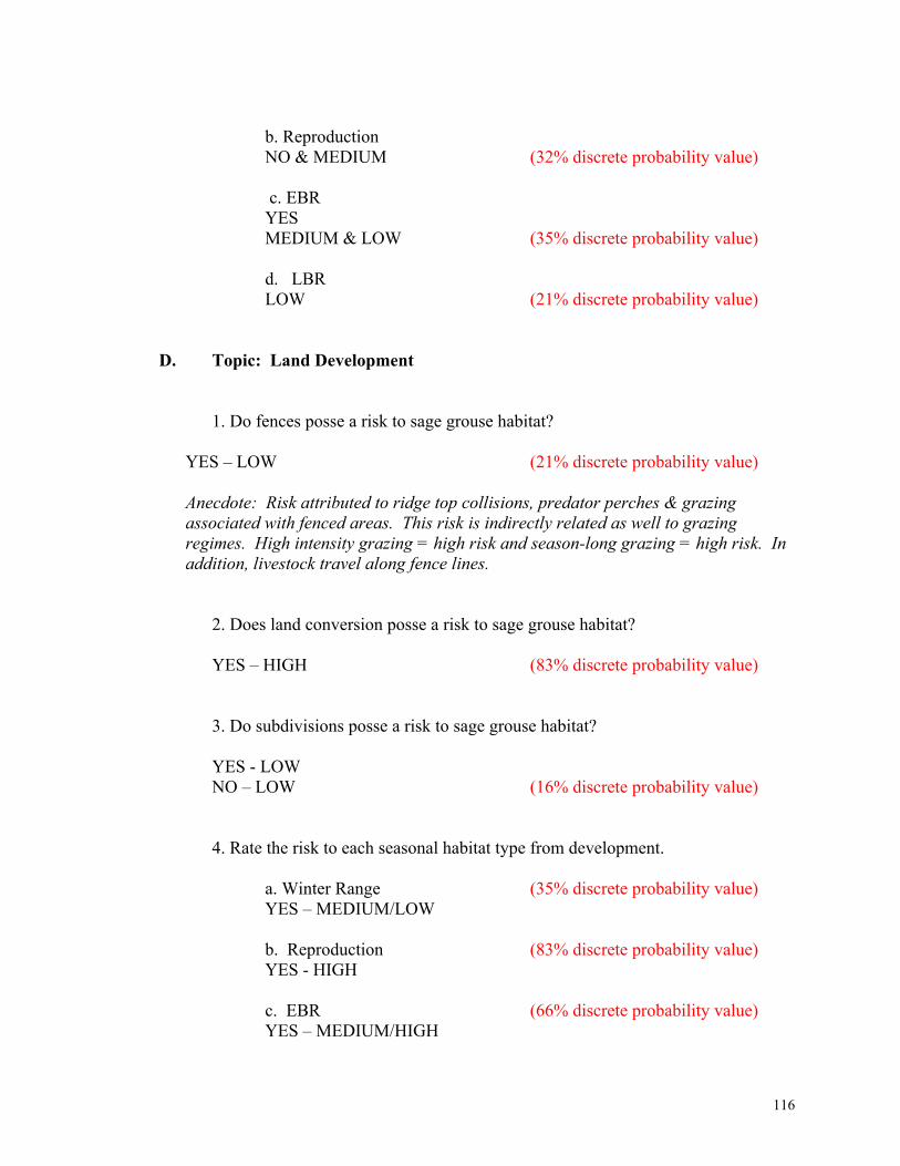
b. Reproduction NO & MEDIUM (32% discrete probability value)
c. EBR
YES MEDIUM & LOW (35% discrete probability value)
d. LBR LOW (21% discrete probability value)
D. Topic: Land Development
1. Do fences posse a risk to sage grouse habitat?
YES – LOW (21% discrete probability value)
Anecdote: Risk attributed to ridge top collisions, predator perches & grazing associated with fenced areas. This risk is indirectly related as well to grazing regimes. High intensity grazing = high risk and season-long grazing = high risk. In addition, livestock travel along fence lines.
2. Does land conversion posse a risk to sage grouse habitat?
YES – HIGH (83% discrete probability value)
3. Do subdivisions posse a risk to sage grouse habitat?
YES - LOW NO – LOW (16% discrete probability value)
4. Rate the risk to each seasonal habitat type from development.
a. Winter Range (35% discrete probability value) YES – MEDIUM/LOW
b. Reproduction (83% discrete probability value) YES - HIGH
c. EBR (66% discrete probability value)
YES – MEDIUM/HIGH
116
e. LBR (21% discrete probability value) YES - LOW
5. At what proximity do houses posse risk to sage grouse habitat
HIGH – (both) (83% discrete probability value) E. Optimal numbers & carrying capacity of landscape for sage grouse? Unknown.
Approximately 10,000 – 12,000 individuals, possibly 15,000 F. Information Sources Personal observation and experience Working relationships with other professionals Professional meetings and conferences Scientific literature Landowners and hunters
117
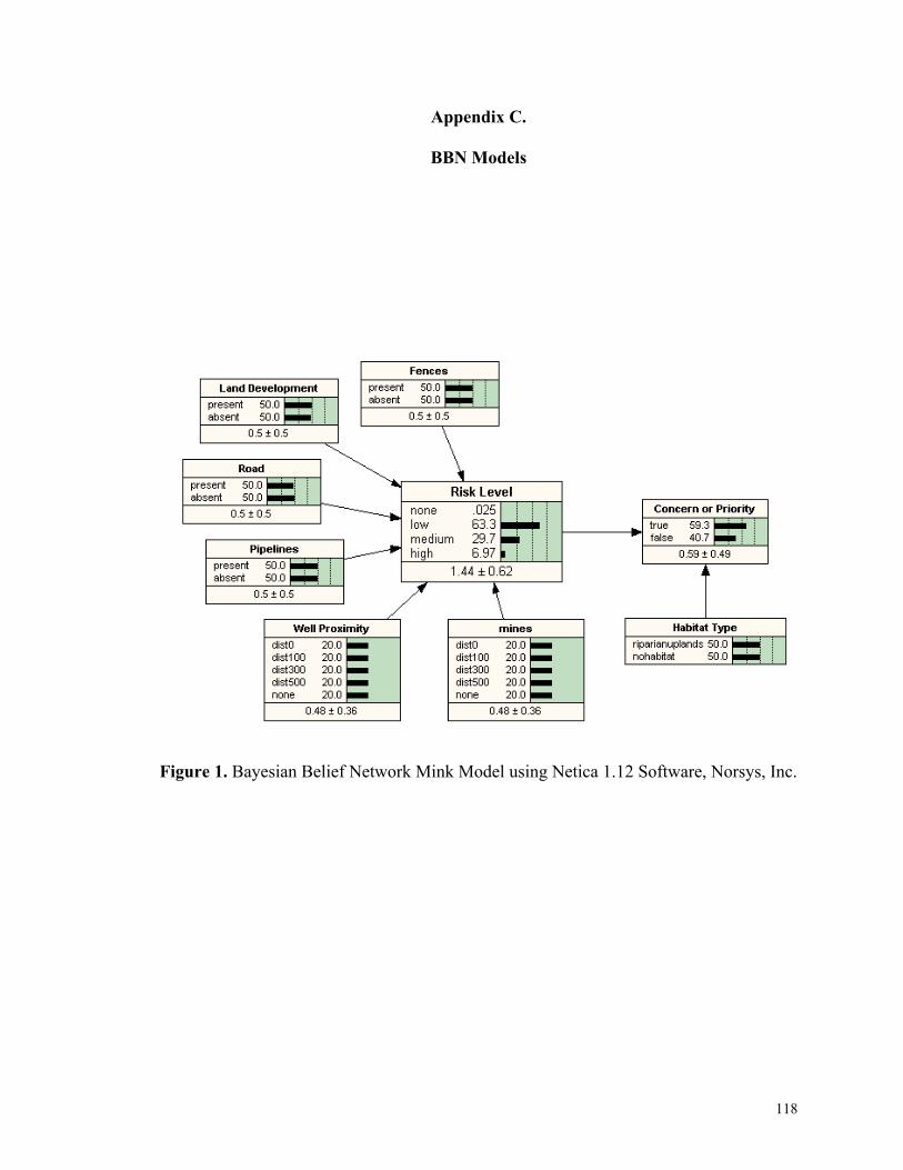
Appendix C.
BBN Models
Figure 1. Bayesian Belief Network Mink Model using Netica 1.12 Software, Norsys, Inc.
118
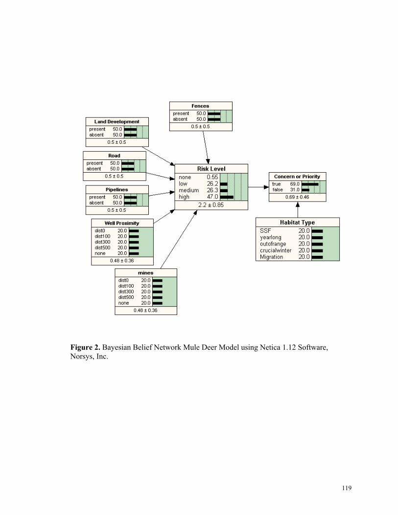
Figure 2. Bayesian Belief Network Mule Deer Model using Netica 1.12 Software, Norsys, Inc.
119
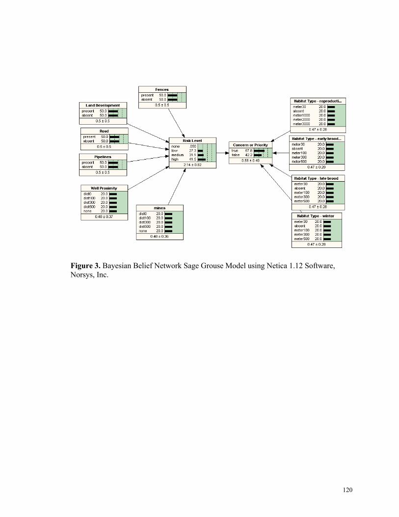
Figure 3. Bayesian Belief Network Sage Grouse Model using Netica 1.12 Software, Norsys, Inc.
120
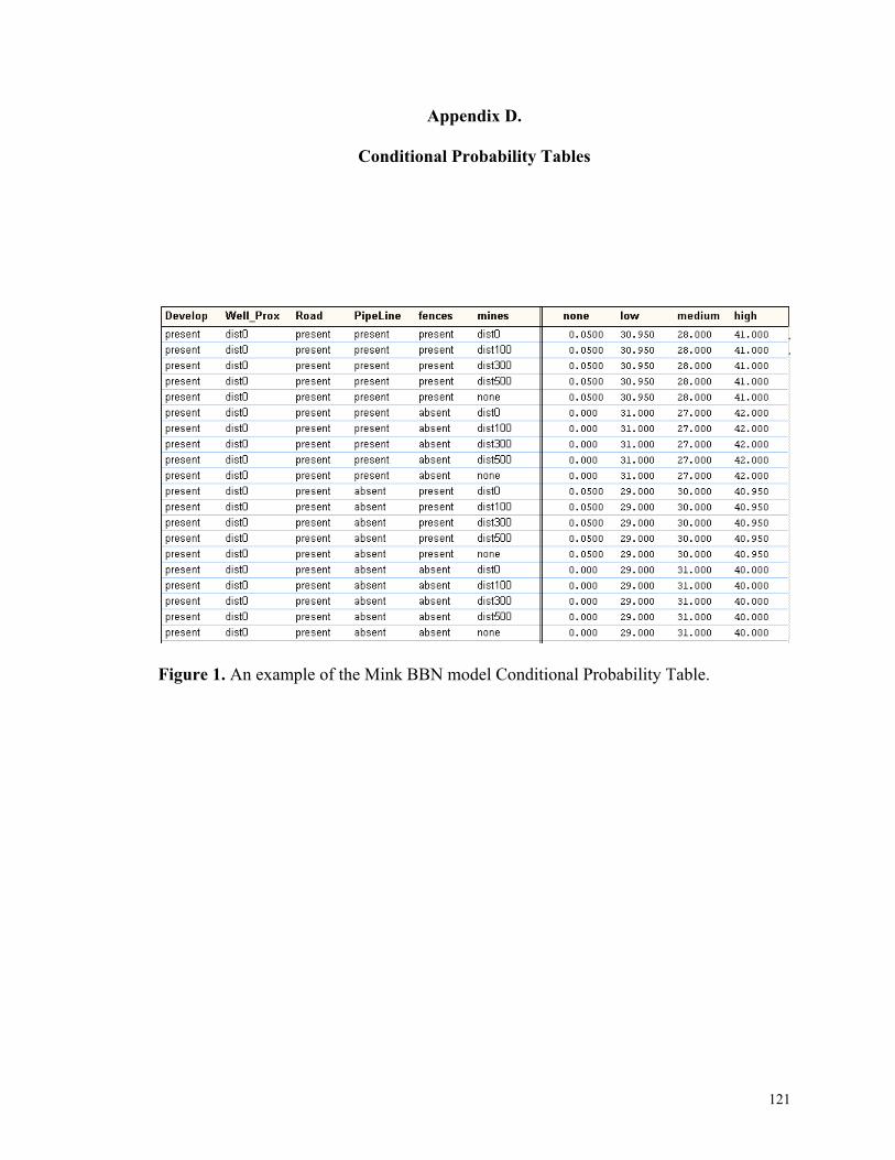
Appendix D.
Conditional Probability Tables
Figure 1. An example of the Mink BBN model Conditional Probability Table.
121
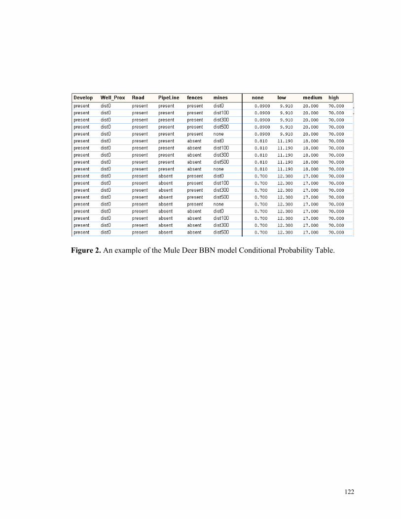
Figure 2. An example of the Mule Deer BBN model Conditional Probability Table.
122
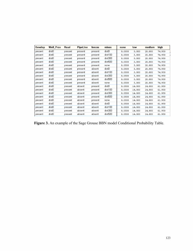
Figure 3. An example of the Sage Grouse BBN model Conditional Probability Table.
123
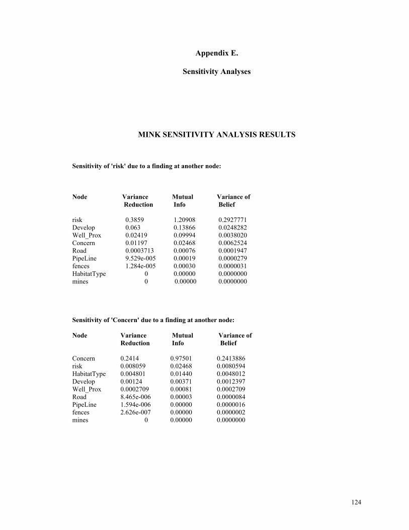
Appendix E.
Sensitivity Analyses
MINK SENSITIVITY ANALYSIS RESULTS
Sensitivity of 'risk' due to a finding at another node:
Node Variance Mutual Variance of Reduction Info Belief risk 0.3859 1.20908 0.2927771 Develop 0.063 0.13866 0.0248282 Well_Prox 0.02419 0.09994 0.0038020 Concern 0.01197 0.02468 0.0062524 Road 0.0003713 0.00076 0.0001947 PipeLine 9.529e-005 0.00019 0.0000279 fences 1.284e-005 0.00030 0.0000031 HabitatType 0 0.00000 0.0000000 mines 0 0.00000 0.0000000 Sensitivity of 'Concern' due to a finding at another node:
Node Variance Mutual Variance of Reduction Info Belief
Concern 0.2414 0.97501 0.2413886 risk 0.008059 0.02468 0.0080594 HabitatType 0.004801 0.01440 0.0048012 Develop 0.00124 0.00371 0.0012397 Well_Prox 0.0002709 0.00081 0.0002709 Road 8.465e-006 0.00003 0.0000084 PipeLine 1.594e-006 0.00000 0.0000016 fences 2.626e-007 0.00000 0.0000002 mines 0 0.00000 0.0000000
124

MULE DEER SENSITIVITY RESULTS
Sensitivity of 'risk' due to a finding at another node:
Node Variance Mutual Variance of
Reduction Info Belief risk 0.7151 1.56649 0.4230569 Concern 0.03786 0.04170 0.0073483 Develop 0.01777 0.02119 0.0043224 Well_Prox 0.01618 0.01818 0.0034372 Road 0.001657 0.00172 0.0003311 PipeLine 0.0002387 0.00035 0.0000443 fences 8.333e-005 0.00009 0.0000149 mines 7.143e-006 0.00002 0.0000030 HabitatType1 0 0.00000 0.0000000 Sensitivity of ‘concern’ due to a finding at another node: Node Variance Mutual Variance of Reduction Info Belief Concern 0.214 0.89346 0.2139949 risk 0.01228 0.04169 0.0122789 HabitatType1 0.00905 0.02888 0.0090504 Develop 0.0003398 0.00115 0.0003397 Well_Prox 0.0002962 0.00099 0.0002962 Road 2.886e-005 0.00010 0.0000289 PipeLine 3.684e-006 0.00001 0.0000037 fences 1.326e-006 0.00000 0.0000014 mines 1.528e-007 0.00000 0.0000001
125
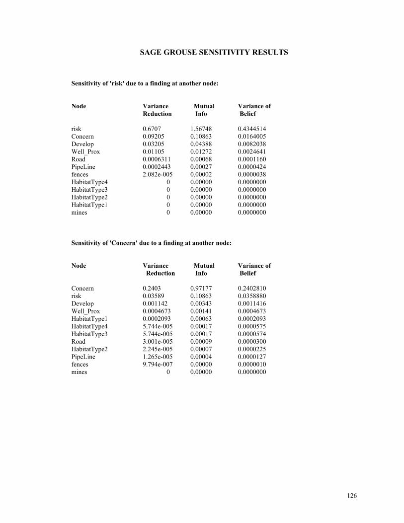
SAGE GROUSE SENSITIVITY RESULTS
Sensitivity of 'risk' due to a finding at another node:
Node Variance Mutual Variance of Reduction Info Belief risk 0.6707 1.56748 0.4344514 Concern 0.09205 0.10863 0.0164005 Develop 0.03205 0.04388 0.0082038 Well_Prox 0.01105 0.01272 0.0024641 Road 0.0006311 0.00068 0.0001160 PipeLine 0.0002443 0.00027 0.0000424 fences 2.082e-005 0.00002 0.0000038 HabitatType4 0 0.00000 0.0000000 HabitatType3 0 0.00000 0.0000000 HabitatType2 0 0.00000 0.0000000 HabitatType1 0 0.00000 0.0000000 mines 0 0.00000 0.0000000
Sensitivity of 'Concern' due to a finding at another node:
Node Variance Mutual Variance of Reduction Info Belief Concern 0.2403 0.97177 0.2402810 risk 0.03589 0.10863 0.0358880 Develop 0.001142 0.00343 0.0011416 Well_Prox 0.0004673 0.00141 0.0004673 HabitatType1 0.0002093 0.00063 0.0002093 HabitatType4 5.744e-005 0.00017 0.0000575 HabitatType3 5.744e-005 0.00017 0.0000574 Road 3.001e-005 0.00009 0.0000300 HabitatType2 2.245e-005 0.00007 0.0000225 PipeLine 1.265e-005 0.00004 0.0000127 fences 9.794e-007 0.00000 0.0000010 mines 0 0.00000 0.0000000
126