Resolution and Depth of Field © Joel A. Levitt, 2008

joelalevitt@comcast.net

CONTENTS

Resolution vs. Depth of Field ……………………............. 2 A Qualitative Understanding …………………………….. 3

Notation ………………………………………….. 3 Diffraction ……………………………………….. 5

Quantitative Definitions ………………………….............. 7 Algebraic Expressions and Numerical Values For Two Point Resolution and Depth of Field …………… 8 Two Point Resolution Illustrations ……………….............. 8 Two Point Resolution …………………….............. 8 Quantization ………………………………………. 10 Noise ……………………………………………… 11 Aberrations ……………………………………………….. 14 Summary …………………………………………………. 15

The Role of the Aperture and of Color …………... 15 Desirable Camera Features ……………………….. 16 Desirable Lens Features …………………………... 16 Useful Procedures ………………………………… 16

Obtain better resolution …………………... 16 Use the best exposure …………….. 16 Use the finest quantization ……….. 17

Reduce noise ……………………… 17 Obtain greater depth of field ……………… 17

2Recently club members have been exchanging questions and information about resolution1 and depth of field2. As a first cut, it may be said that the larger the f-number (that is, the smaller the lens aperture) the worse the resolution and the greater the depth of field. Both resolution and depth of field are determined by diffraction (the tendency of light to spread out like a wave rather than travel along straight lines or rays). But, there are other factors to be considered, too: the color of the details to be captured, the density of pixels on your sensor array or the grain size of your film; the way that your camera quantifies3 the picture (using 8bit or 16 bit or still larger numbers); the noise of your recording material (be it film or a charged coupled array); the light scattered by your lens, and the aberrations introduced by your lens and where the details to be captured are located in the photo (in the center or at the edge). This note attempts to provide easily understood explanations of these factors. Remember, you don’t have to have the time to read or to absorb the material in this note in order to take great photos. Your esthetic perceptions and your imagination are far more important. But, understanding will help you to choose a camera, and it may frequently help you to actually take the pictures that you intend to take. RESOLUTION vs. DEPTH OF FIELD There is a trade-off between resolution and depth of field. The configuration shown in Figure 1 was used to make photos which illustrate this trade-off.

Figure 1: Configuration used to photograph a metric ruler oriented at 45o to the optic axis. NOTES: 1. Resolution relates to how small object-detail (such as bark texture or facial wrinkles) can be and still be seen in the finished photo. 2. Depth of Field -- Photos contain usefully clear images of objects located in the in-focus plane and of those that are some distance in front of and some distance behind the in-focus plane. Depth of Field is the sum of these distances. 3. Picture Quantification – Your digital camera measures the light that falls on each sensor and forwards the resulting number to its processing electronics.

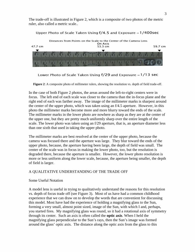
3The trade-off is illustrated in Figure 2, which is a composite of two photos of the metric ruler, also called a metric scale..

Figure 2: A composite photo of millimeter rulers, showing the resolution vs. depth of field trade-off.

In the case of both Figure 2 photos, the areas around the left-to-right centers were in focus. The left end of each scale was closer to the camera than the in-focus plane and the right end of each was farther away. The image of the millimeter marks is sharpest around the center of the upper photo, which was taken using an f/4.5 aperture. However, in this photo the millimeter marks become more and more blurry toward the ends of the scale. The millimeter marks in the lower photo are nowhere as sharp as they are at the center of the upper one, but they are pretty much uniformly sharp over the entire length of the scale. The lower photo was taken using an f/29 aperture, that is, an aperture diameter less than one sixth that used in taking the upper photo. The millimeter marks are best resolved at the center of the upper photo, because the camera was focused there and the aperture was large. They blur toward the ends of the upper photo, because, the aperture having been large, the depth of field was small. The center of the scale was in focus in making the lower photo, too, but the resolution is degraded there, because the aperture is smaller. However, the lower photo resolution is more or less uniform along the lower scale, because, the aperture being smaller, the depth of field is larger. A QUALITATIVE UNDERSTANDING OF THE TRADE OFF Some Useful Notation A model lens is useful in trying to qualitatively understand the reasons for this resolution vs. depth of focus trade off (see Figure 3). Most of us have had a common childhood experience that we can draw on to develop the words that are convenient for discussing this model. Most have had the experience of holding a magnifying glass to the Sun, forming a very small, almost point sized, image of the Sun, with which I and, perhaps, you started fires. My magnifying glass was round, so it had a rotational axis of symmetry through its center. Such an axis is often called the optic axis. When I held the magnifying glass perpendicular to the Sun’s rays, then the Sun’s image was formed around the glass’ optic axis. The distance along the optic axis from the glass to this

4image is called the focal length of the magnifying lens. The point on the optic axis that was at the center of this image is called the focal point, and the plane that was perpendicular to the optic axis and contained the spot-like image is called the focal plane. When I flipped the lens over, the same image formed. So each lens has two focal lengths, one on each side of the lens and, correspondingly, two focal planes. All this fun resulted from the fact that image forming lenses squeeze parallel light, also called collimated light, into a small area around its focal point. The sun is so far away that the light that was incident upon the lens (i.e., the sunlight that fell upon the lens) was close to parallel, hence the hotspot image. Forming a small hotspot at the focal point using collimated incident light works in reverse, too. If a transilluminated pinhole is located at a focal point of a lens, then the lens will produce a collimated beam of light. We can now use the bolded words just defined to understand the model lens shown in Figure 3.

Figure 3: Optics notation.

Figure 3 shows the image of a point source being formed by a two element lens through a circular aperture. An approximate point source can be formed by transilluminating a pinhole formed in a piece of metal foil. The elements of the lens are themselves lenses, thin image-forming lenses. The pinhole is located at the front focal point of the first element, and the two-element lens assembly forms an image of the pinhole around the back focal point of the second element. This happens because, just like our magnifying glasses, the first element produces a collimated beam from the light that comes through the pinhole, and the second element brings that collimated beam to a focus around its back focal point. . In fact, all the points of the front focal plane of the first element are in focus on the back focal plane of the second element. So, in this case, the front focal plane of the first element can be called the object plane and the back focal plane of the second element can be called the image plane. If light traveled along straight lines, then the image of the pin hole would, except for magnification, look just like the pin hole, itself. This idealized image is called the geometric image of the pinhole. Light, however, travels like a wave. So the image is

5spread out and distorted. This spreading and distorting process is called diffraction and is mostly controlled by the size of the circular aperture. In such cases the image is said to be aperture-limited. In Figure 3, the circular aperture is centered on the optic axis and is located in the coincident back focal plane of the first element and front focal plane of the second element. This location is chosen because it makes calculations easier, but it does not affect the generality of the following discussion. Taking care of some details, the focal lengths of the first and second elements are designated f and f’, respectively. The transverse magnification (the magnification of line segments lying in the object plane) of the two element lens is

mt = f’/f, (1)

and its axial magnification (the magnification of a line segment in the object space that is parallel to the optic axis) is

ma = mt2. (2)

The axial magnification describes the position of an image toward or away from the lens. If a point located at z ≠ 0 is imaged at z’, then the axial magnification is ma = z’/z. Finally, the size of the aperture, diameter = 2a, is measured by the

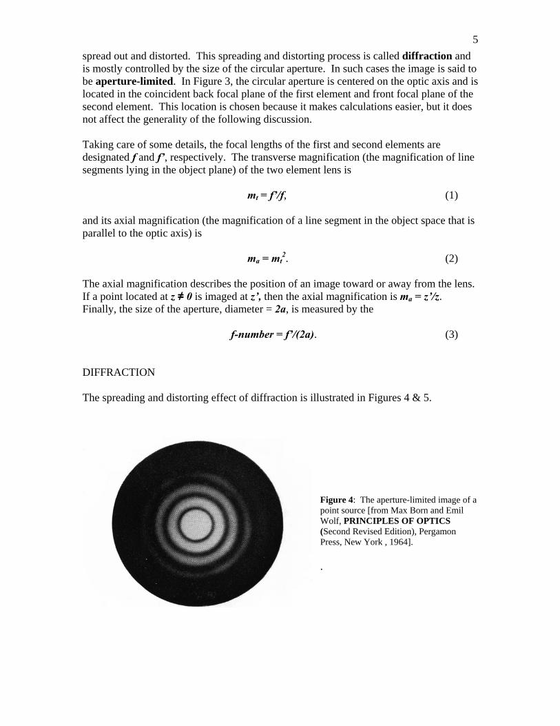
f-number = f’/(2a). (3) DIFFRACTION The spreading and distorting effect of diffraction is illustrated in Figures 4 & 5.

Figure 4: The aperture-limited image of a point source [from Max Born and Emil Wolf, PRINCIPLES OF OPTICS (Second Revised Edition), Pergamon Press, New York , 1964].

.

6An approximate point-source located on or near the optic axis of a lens and imaged through an aperture does not produce a point image. Instead, as shown in the photograph in Figure 4, the image is a bright disc surrounded by bright rings. In the absence of noise, the intensity (the light power per unit area) is zero on some circle within each of the dark rings, and the larger the f-number, the smaller the aperture and the larger the bright disc. The distance between two image points will be proportional to mt (Eq.1), and the diameter of their bright discs will be proportional to the f-number (Eq. 3), so the ratio of these quantities is a useful predictive number.

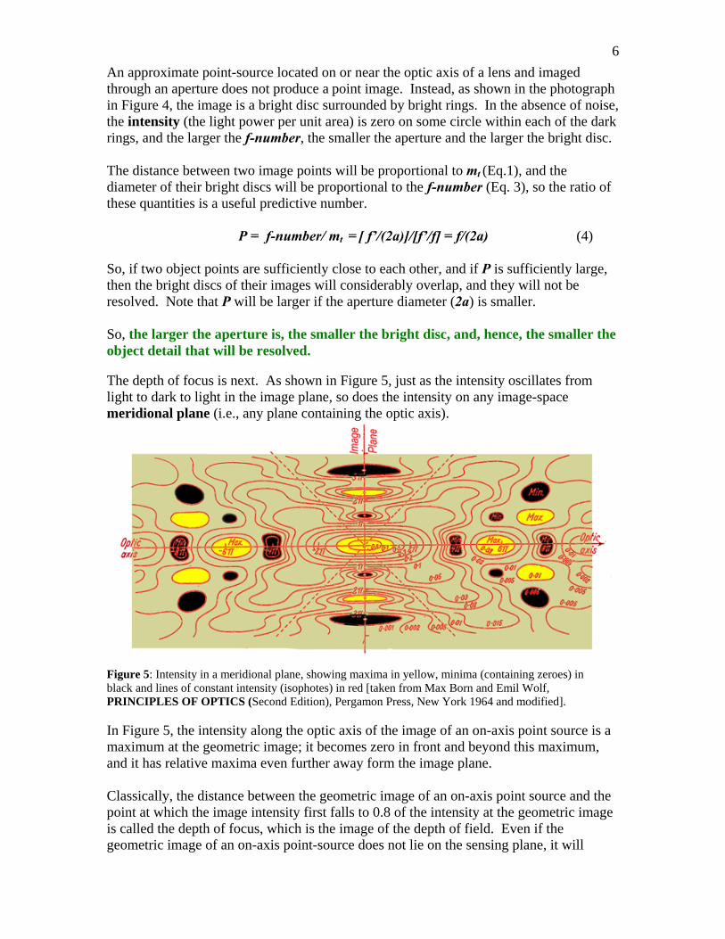
P = f-number/ mt = [ f’/(2a)]/[f’/f] = f/(2a) (4) So, if two object points are sufficiently close to each other, and if P is sufficiently large, then the bright discs of their images will considerably overlap, and they will not be resolved. Note that P will be larger if the aperture diameter (2a) is smaller. So, the larger the aperture is, the smaller the bright disc, and, hence, the smaller the object detail that will be resolved. The depth of focus is next. As shown in Figure 5, just as the intensity oscillates from light to dark to light in the image plane, so does the intensity on any image-space meridional plane (i.e., any plane containing the optic axis).

Figure 5: Intensity in a meridional plane, showing maxima in yellow, minima (containing zeroes) in black and lines of constant intensity (isophotes) in red [taken from Max Born and Emil Wolf, PRINCIPLES OF OPTICS (Second Edition), Pergamon Press, New York 1964 and modified]. In Figure 5, the intensity along the optic axis of the image of an on-axis point source is a maximum at the geometric image; it becomes zero in front and beyond this maximum, and it has relative maxima even further away form the image plane. Classically, the distance between the geometric image of an on-axis point source and the point at which the image intensity first falls to 0.8 of the intensity at the geometric image is called the depth of focus, which is the image of the depth of field. Even if the geometric image of an on-axis point-source does not lie on the sensing plane, it will

7appear to be in focus in the fully digitized image provided that its geometric image lies within the depth of focus of the sensing plane. So, the smaller the aperture, the greater the depth of field. The resolution vs. depth of field trade-off has been illustrated and the underpinning diffraction process has been explained qualitatively. But just how far apart do two object points have to be to be resolved? And, given an f-number, what will the depth of field be? And, what camera properties and settings affect resolution and depth of field? These questions will be answered semi-quantitatively in the following after again referring to Figure 3 and defining some more quantitative terms. QUANTITATIVE DEFINITIONS 1. From left to right, that is, from the object space to the image space,the f-numbers of the first and second lens elements are n=f/2a and n’=f ’/2a, respectively. 2. The focal length of the composite lens is F, and its f-number is N=F/2a. 3. Intensity, I, the light power per unit area, varies over the diffraction-blurred image. 4. λ is the wavelength of the illuminating light.

In the case of blue green light, λ = 0.5 micrometers (thousandths of a millimeter). In the case of deep red light, λ = 0.633 micrometers.

5. r is the distance from the image origin (the point of intersection of the image plane and the optic axis) to any other point in the image plane. 6. R = (πr)/(Nλ) is the dimensionless distance from image origin to any other `point in the image plane. In the case of an object consisting of an on-axis point-source, the relative intensity in the image plane is

I(R)/I0 = [J1(R)/R]2, (5)

where: I0 is the intensity at R = 0, and J1(R) is the first order Bessel function of the first kind (if interested, to see a graph of J1(R) go to http://en.wikipedia.org/ wiki/Image:Bessel_Functions_%281st_Kind%2C_n%3D0%2C1%2C2%29.svg). 7. Ro = 3.8 is the dimensionless distance to the first zero of I(R)/I0. Classically, the images of two point-sources are said to be resolved if their geometric images are at least Ro apart. 8. ro = NλR0/π is the distance to the first zero of I(R)/I0. 9. y’ is distance measured along the y’-axis in the image plane. 10. Y’ = (πy’)/(Nλ) is the dimensionless distance measured along the y’-axis in the image plane. 11. z is distance measured from the image plane parallel to the optic axis. 12. Z = πz / (8N2λ) is the dimensionless distance measured from the image plane parallel to the optic axis. In the case of an object consisting of an on-axis point-source, the relative intensity in the along the optic axis is

I(0,Z)/I0 = [Sin(Z)/Z]2 13. Z0.8 = 0.8 is the dimensionless distance to the point at which I(0,Z)/I0 = 0.8. Classically, a point-source is considered to be in focus if its geometric image falls within the interval: -Z0.8 to Z0.8.

814. zo.8 = 8N2λ Z0.8/π is the distance to the point at which I(0,Z)/I0 = 0.8. ALGEBRAIC EXPRESSIONS AND NUMERICAL VALUES FOR TWO POINT RESOLUTION AND DEPTH OF FIELD So, we have the following salient points. The resolution improves as N gets smaller and is proportional to N, and the depth of field increases as N gets larger and is proportional to N2, and Two object point-sources are said to be resolved if their geometric images are at least 1.21Nλ apart, and An object point-source is said to be within the depth of focus if its geometric image is within 2.04N2λ of the image plane. These points are evaluated numerically in the following tables.

ro zo.8 N 4.5 29 4.5 29

λ = 0.5 micrometers (µm) 0.0027 mm

0.0175 mm

0.0207 mm

0.8578 mm

λ = 0.633 micrometers (µm) 0.0034 mm

0.0222 mm 0.0261 1.0860

mm Suppose that the complete image is formed by imaging a field 3m across onto a sensor array 30mm across. Then the transverse magnification is 1/100, and, therefore, the axial magnification is 1/10,000. Given these magnifications, the object-space separation between just resolvable points, so, and the depth of field are tabulated below.

Transverse Magnification = 1/100 Axial Magnification = 1/10,000

so Depth of Field N 4.5 29 4.5 29

λ = 0.5 micrometers (µm) 0.27 mm 1.75 mm 20.7 cm 8.57 m

λ = 0.633 micrometers (µm) 0.34 mm 2.22 mm 26.1 cm 10.86 m

TWO POINT RESOLUTION ILLUSTRATIONS Some desirable operating procedures and camera and lens characteristics can be evinced from the following illustrations of the two point image intensity, in which the geometric images of the two points are located on or near the y’-axis and are 0.5Ro, 0.79Ro and Ro apart. The intensity of an image of an on-axis point-source is graphed in Figure 6, and that of the image of two point-sources with geometric images 0.5Ro apart is graphed in Figure 7.

9When more point-sources than one are imaged, the intensity at any point in the image plane is just the sum of the intensities of each of the images at that point.

Figure 6 Figure 7 The differences between the single point image and the two point image are minor. The two point intensity peak is some what broader and the two point intensity does not reach zero. In the absence of noise, the presence of two image points can be extracted from Figure 7, but this takes fancy and generally unavailable computer calculations. For the purposes of photographers, the distance of 0.5Ro between the points is too small to permit them to be resolved. If otherwise unresolved points must be resolved, then the photographer may be able to resolve them by using a larger aperture (that is, a smaller N), provided the resulting depth of field is acceptable. If otherwise unresolved points can be resolved by using a larger aperture, but the resulting depth of field is too small, then the photographer may be able solve this problem by making several photographs, each focused on a different object plane and merge them with Photoshop. If the geometric images of the point-sources are 0.79Ro apart, then the image intensity, shown in Figure 8, is qualitatively different from that shown in Figure 6.

10

Figure 8

The Figure 8 intensity peak is considerably broader, and there is a dip at Y’ = 0. This dip is too small to be observed in Figure 8, but it can be seen in Figure 9, a magnified view of Figure 8 around (Y’ = 0, I = 1.0).

Figure 9

A discussion of Figure 9 provides an opportunity to define V, visibility, and to discuss some roles played by noise, exposure, quantization, sensor dynamic range, and sensor density. V is a local measure, that is, it changes from region to region over an image.

V = (Imax – I min)/(Imax + Imin),

11where: Imax is I at a relative maximum, and I min is I at an adjacent relative minimum. The visibility of the Figure 9 dip is

V = (1 – 0.999579358) / (1 + 0.999579358) = 0.00021, which is so small that the dip is generally considered undetectable. However, it may be detected under certain favorable conditions. First there must be no or almost no noise. The deleterious effect of noise is illustrated in Figure 10.

Figure 10: Gaussian noises with different average powers have been added to parallel rulings, each with approximately the same period but with different visibilities. The noise is seen to obscure low visibility structure much more than high visibility structure. There is usually some noise in the signal generated by each sensor. This noise is a random variation in time of the sensor signal. It results from noise in the light illuminating the sensor and from thermal effects in the sensor itself and in its conditioning electronics. If the average noise power in the fully digitized image is comparable to or greater than the magnitude of the dip, then there will be no chance of detecting the dip. Most noise of concern is additive, that is, the effective input to the sensor, In, is the sum of the signal, I, and the noise, ν:

In = I(t) + ν(t)

12Resolution is improved by decreasing the noise relative to the signal. Usually the noise varies much more rapidly than the signal. So, many cameras include a desirable low-pass frequency filter to reduce the noise. The remaining noise can be reduced by time averaging. Taking I to be constant and denoting the time averaged noise by < ν >, the effective exposure, E, is:

E = τI + < ν >τ , where: τ is the exposure time. This is beneficial, because the exposure signal, τI, increases linearly with τ, while < ν >τ is proportional to 1/ τ½. So, it is often beneficial to use a smaller aperture (reducing I, which is proportional to the aperture area) or a slower speed setting (ISO) and a longer exposure time. Unfortunately, there is another kind of noise that can only be reduced by spatial averaging, that is blurring, which also degrades resolution. This noise results from light scattered by the lens that adds a time-invariant signal to I, and this addition is different for sensors in different locations in the sensor array. All material media scatter, but some optical materials scatter much less than others. So, it is desirable to have low scatter lenses. If finally the lens scattering noise is too great, the photographer may be able to solve this problem by making several photographs, each centered at a different point in the object plane, and merge them with Photoshop. The second favorable condition has to do with a relationship between exposure and sensor dynamic range. The variations in intensity from image point to image point carry all the information in the image. In some sense these variations are the image. The greater the peak intensities at image points, the greater the variations in intensity and the easier it is to measure them. When a sensor is illuminated, then, up to a cutoff intensity, the sensor produces an electrical current that is proportional to the illuminating intensity, and the sensor associated electronics integrate this current, producing a voltage that is proportional to the exposure. If the intensity exceeds the cutoff more and more, then the sensor will produce smaller and smaller current increments in response to successive intensity increments, and its overall response will be nonlinear. Therefore, the useful intensity range is:

0 ≤ I ≤ I cutoff , corresponding to the useful (that is, linear) dynamic range of the sensors. So, cameras with larger sensor dynamic ranges are more desirable.

13Also, it is useful to set the aperture so that I falls in this range and to use the exposure time such that the exposure at the most intense image point is just at the exposure cutoff of the sensor. This is why it is recommended that the exposure used produce a histogram that borders the right boundary of the Photoshop histogram window. Most cameras measure image point exposures by dividing the exposure dynamic range into equal intervals and determining into which interval the exposure at an image point falls. These intervals are called quantization intervals, and the measurement process is called quantization. In the case of 8-bit quantization there are 255 quantization intervals. In the case of 16-bit quantization there are (256 x256) – 1 = 65,535 quantization intervals. In Figure 9 it is shown that, all other conditions favorable, using 8-bit quantization the dip will hardly ever be detected in the final image, because the quantization interval is so much larger than the dip. However, the dip will be detected if 16-bit quantization is used. So, if some desired small feature is not captured in a photo, try a finer quantization scheme. Classically, it was said that two points will be resolved if their geometric images are at least Ro apart. This is the case shown in Figure 11.

Figure 11.

14In the classically just-resolved Figure 11 case the dip visibility is:

V = 0.144.

There is one more camera feature that is important in capturing small features – sensor density. Imagine in Figure 11 that the sensors are 2Ro apart, then the dip cannot be captured. But, if the sensor separation is Ro/10, then there is no problem. So, greater sensor density is better. However, remember – if you wish to capture a picture of a particular size, greater sensor data means more pixels. ABERRATIONS To this point, this note has not touched on lens aberrations, and the discussion has been limited to the images of point-sources located on or near the optic axis. Now this omission will be remedied. There are three prominent aberrations: chromatic aberration; spherical aberration, and coma. Chromatic aberration is the focusing of different colors in different planes. Most camera lenses of most manufacturers are made using several elements of materials with different indices of refraction. This is done to eliminate chromatic aberration. And, most are sufficiently successful for photography. The several elements of most camera lenses are usually of different shapes in order to limit spherical aberration and coma. These aberrations, shown in Figures 12 and 13, are produced by areas of the lens near its outer margin, which image point-sources into rings or ring segments concentric about the their geometric images.

15Figure 12: Primary spherical aberration is an image defect produced by the lens that broadens the

aperture-limited image of point-sources on or near the optic axis.

Figure 13: Primary coma is an image defect produced by the lens that stretches the aperture-limited image of point-sources that are far form the optic axis. These images are stretched away from the optic axis along the lines joining the optic axis and the geometric images of the point-sources. SUMMARY The Role of the Aperture and of Color Resolution improves as N gets smaller and is proportional to N, and the depth of field increases as N gets larger and is proportional to N2. Two object point-sources are said to be resolved if their geometric images are at least 1.21Nλ apart, and An object point-source is said to be within the depth of focus if its geometric image is within 2.04N2λ of the image plane.

16

ro zo N 4.5 29 4.5 29

λ = 0.5 micrometers (µm) 0.0027 mm

0.0175 mm

0.0207 mm

0.8578 mm

λ = 0.633 micrometers (µm) 0.0034 mm

0.0222 mm 0.0261 1.0860

mm

(Axial Magnification) = (Transverse Magnification)2

Transverse Magnification = 1/100 Axial Magnification = 1/10,000

so Depth of Field N 4.5 29 4.5 29

λ = 0.5 micrometers (µm) 0.27 mm 1.75 mm 20.7 cm 8.57 m

λ = 0.633 micrometers (µm) 0.34 mm 2.22 mm 26.1 cm 10.86 m

Desirable Camera Features:

a low-pass electronic noise reduction filter; greater sensor density; sensors with greater linear dynamic range;

low noise sensors, and 16-bit or finer quantization. Desirable Lens Features: made of lower scatter optical materials; better corrected for primary spherical aberration and coma; Useful Procedures: To obtain better resolution:

use a larger aperture, provided the reduction in depth of field is acceptable; set the aperture so that I falls in the linear range (0 ≤ I ≤ I cutoff ) and to use the exposure time such that the exposure at the most intense image point is just at the exposure cutoff of the sensor;

17try a finer quantization scheme; reduce noise:

to reduce time-dependent noise use lower speed (ISO) settings and/or smaller apertures to increase exposure time, provided increased motion blur and/or degraded resolution are acceptable;

to reduce space-dependent noise (such as may arise from lens scattering), make several photographs -- each centered at a different point in the object plane and merge them with Photoshop;

To obtain greater depth of field:

use a smaller aperture, provided that degraded resolution is acceptable, and to obtain a usefully large effective depth of field, even though the depth of field produced by using the aperture needed to resolve desired detail is too small, make several photographs, each focused on a different object plane and merge them with Photoshop.