University of California

Los Angeles

Resource Allocation for Sources with CorrelatedData

A dissertation submitted in partial satisfaction

of the requirements for the degree

Doctor of Philosophy in Electrical Engineering

by

Dorna Bandari

2011

c� Copyright by

Dorna Bandari

2011

The dissertation of Dorna Bandari is approved.

Mario Gerla

Lieven Vandenberghe

John Villasenor

Gregory J. Pottie, Committee Chair

University of California, Los Angeles

2011

ii

To my parents for all their support.

iii

Table of Contents

1 Introduction . . . . . . . . . . . . . . . . . . . . . . . . . . . . . . . . 1

1.1 Cases Considered . . . . . . . . . . . . . . . . . . . . . . . . . . . 2

1.1.1 Correlation-aware Design . . . . . . . . . . . . . . . . . . . 2

1.1.2 Multi-view Video Systems . . . . . . . . . . . . . . . . . . 2

1.1.3 Cellular Systems . . . . . . . . . . . . . . . . . . . . . . . 3

1.2 Contributions . . . . . . . . . . . . . . . . . . . . . . . . . . . . . 4

1.3 Organization . . . . . . . . . . . . . . . . . . . . . . . . . . . . . 4

2 Technical Background . . . . . . . . . . . . . . . . . . . . . . . . . . 6

2.1 Convex Optimization . . . . . . . . . . . . . . . . . . . . . . . . . 6

2.1.1 General Formulation . . . . . . . . . . . . . . . . . . . . . 6

2.1.2 Augmented Lagrangian Dual Decomposition Method . . . 8

2.2 Multiple Access Protocols . . . . . . . . . . . . . . . . . . . . . . 8

2.2.1 CDMA . . . . . . . . . . . . . . . . . . . . . . . . . . . . . 9

2.2.2 FDMA . . . . . . . . . . . . . . . . . . . . . . . . . . . . . 9

2.3 Resource Allocation Problem . . . . . . . . . . . . . . . . . . . . . 9

2.3.1 General Formulation . . . . . . . . . . . . . . . . . . . . . 10

2.3.2 Multi-cell systems . . . . . . . . . . . . . . . . . . . . . . . 11

2.4 Correlated Sources . . . . . . . . . . . . . . . . . . . . . . . . . . 11

2.4.1 Joint Rate-Distortion Region . . . . . . . . . . . . . . . . 12

3 Correlation used in resource allocation for single-cell networks 13

iv

3.1 Introduction . . . . . . . . . . . . . . . . . . . . . . . . . . . . . . 13

3.2 Problem Settings . . . . . . . . . . . . . . . . . . . . . . . . . . . 16

3.2.1 Framework . . . . . . . . . . . . . . . . . . . . . . . . . . 16

3.2.2 Problem Formulation . . . . . . . . . . . . . . . . . . . . . 16

3.3 Optimal Resource Allocation . . . . . . . . . . . . . . . . . . . . . 18

3.3.1 Aggregate Utility Model . . . . . . . . . . . . . . . . . . . 18

3.3.2 Optimization Solution . . . . . . . . . . . . . . . . . . . . 20

3.4 Simulations . . . . . . . . . . . . . . . . . . . . . . . . . . . . . . 23

3.4.1 Simulation Setup . . . . . . . . . . . . . . . . . . . . . . . 23

3.4.2 Correlated Video Model Validation . . . . . . . . . . . . . 24

3.4.3 Resource Allocation Performance . . . . . . . . . . . . . . 26

3.5 Conclusion . . . . . . . . . . . . . . . . . . . . . . . . . . . . . . . 28

4 ICon: Multi-cell OFDMA based resource allocation using inter-

ference concentration . . . . . . . . . . . . . . . . . . . . . . . . . . . . 30

4.1 Introduction . . . . . . . . . . . . . . . . . . . . . . . . . . . . . . 30

4.2 Related Work . . . . . . . . . . . . . . . . . . . . . . . . . . . . . 33

4.3 Optimization Problem . . . . . . . . . . . . . . . . . . . . . . . . 35

4.3.1 ICon . . . . . . . . . . . . . . . . . . . . . . . . . . . . . . 37

4.3.2 Channel and Power Assignment in Each Cell . . . . . . . . 38

4.4 Adaptation of ICon . . . . . . . . . . . . . . . . . . . . . . . . . . 39

4.5 Simulations . . . . . . . . . . . . . . . . . . . . . . . . . . . . . . 41

4.6 Conclusion . . . . . . . . . . . . . . . . . . . . . . . . . . . . . . . 45

v

5 Correlation used in resource allocation for Multi-cell networks 46

5.1 Introduction . . . . . . . . . . . . . . . . . . . . . . . . . . . . . . 46

5.2 Related Work . . . . . . . . . . . . . . . . . . . . . . . . . . . . . 50

5.3 Problem Formulation . . . . . . . . . . . . . . . . . . . . . . . . . 51

5.3.1 Resources . . . . . . . . . . . . . . . . . . . . . . . . . . . 52

5.3.2 Rate-Distortion Region . . . . . . . . . . . . . . . . . . . . 53

5.3.3 Optimization Problem . . . . . . . . . . . . . . . . . . . . 55

5.4 Proposed Three Phase Solution . . . . . . . . . . . . . . . . . . . 56

5.4.1 Inter-Cell Resource Management . . . . . . . . . . . . . . 57

5.4.2 Grouping of Correlated Sources . . . . . . . . . . . . . . . 62

5.4.3 Intra-Cell Scheduling . . . . . . . . . . . . . . . . . . . . . 67

5.5 Simulations . . . . . . . . . . . . . . . . . . . . . . . . . . . . . . 70

5.6 Conclusion . . . . . . . . . . . . . . . . . . . . . . . . . . . . . . . 73

6 Concluding Remarks . . . . . . . . . . . . . . . . . . . . . . . . . . 77

References . . . . . . . . . . . . . . . . . . . . . . . . . . . . . . . . . . . 79

vi

List of Figures

1.1 In multi-user networks many users share the common radio resources. 1

1.2 Cellular systems. . . . . . . . . . . . . . . . . . . . . . . . . . . . 3

2.1 A convex function of one variable. . . . . . . . . . . . . . . . . . . 7

3.1 General framework: N sources stream live video to the base station

on a shared bottleneck channel, before it is forwarded to the decoder. 14

3.2 Breakdancing sequence. . . . . . . . . . . . . . . . . . . . . . . . 25

3.3 Breakdancing sequence. . . . . . . . . . . . . . . . . . . . . . . . . 26

3.4 Breakdancing sequence. . . . . . . . . . . . . . . . . . . . . . . . . 27

3.5 Average quality for 3 sources, Normalized Noise power (dBm) =

[23, 17, 23]. . . . . . . . . . . . . . . . . . . . . . . . . . . . . . . 28

3.6 Average quality for 3 sources, Normalized Noise power (dBm) =

[27, 17, 20]. . . . . . . . . . . . . . . . . . . . . . . . . . . . . . . 28

4.1 An example of Interference Power Profiles (IPPs) set by ICon

method for cell types 1 and 2 in a hexagonal cellular network. . . 33

4.2 Transmit power profiles for each cell type in a hexagonal cellular

network, using SFR. The colored section of each cell only has access

to the parts of the spectrum with the matching color, the inner

sections of cells have access to the whole spectrum. . . . . . . . . 34

4.3 Interference Power Profile (IPP) for cell u. Green curve is the IPP

that cell k has to respect for cell u. . . . . . . . . . . . . . . . . . 40

vii

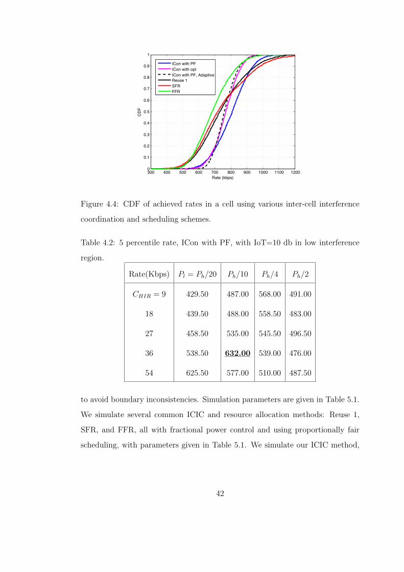
4.4 CDF of achieved rates in a cell using various inter-cell interference

coordination and scheduling schemes. . . . . . . . . . . . . . . . . 42

4.5 Close-up of Fig. 4.4 demonstrating the five percentile rate achieved

in each of the methods. . . . . . . . . . . . . . . . . . . . . . . . . 43

4.6 Evolution of 5 percentile rate when the ICon adaptation is allowed.

ICon with PF scheduling for site to site = 130 m, users per cell:

19-21, uniformly distributed. . . . . . . . . . . . . . . . . . . . . . 44

5.1 3 neighboring cells shown, with base stations in the center of each

cell. Sources are grouped in correlated groups of size 2. . . . . . . 47

5.2 System overview. . . . . . . . . . . . . . . . . . . . . . . . . . . . 52

5.3 Scheduler in the base stations. . . . . . . . . . . . . . . . . . . . . 56

5.4 An example of Interference Power Profiles (IPPs) set by ICon

method for cell types 1 and 2 in a hexagonal cellular network. . . 58

5.5 Interference Power Profile (IPP) for cell u. Green curve is the IPP

that cell k has to respect for cell u. . . . . . . . . . . . . . . . . . 59

5.6 Example of output of grouping algorithms. (a) is the result of the

distance based grouping method without outer priority (OP), while

(b) is the groups resulting from distance based method with OP.

The effects of OP can be seen by observing the change of grouping

that occurs around the source drawn in red. (c) demonstrates the

grouping results from the three per set distance based with OP

method. . . . . . . . . . . . . . . . . . . . . . . . . . . . . . . . . 61

5.7 Trade-off of distortions for two correlated users. . . . . . . . . . . 63

5.8 Diminishing returns of increasing correlated set size on distortion. 67

viii

5.9 Inter-cell scheduling methods. . . . . . . . . . . . . . . . . . . . . 72

5.10 Closeup of distortion CDF of inter-cell resource management meth-

ods.. . . . . . . . . . . . . . . . . . . . . . . . . . . . . . . . . . . 73

5.11 Comparison of distortion CDF in D-PF vs R-PF vs OPT scheduling. 74

5.12 Source grouping methods. . . . . . . . . . . . . . . . . . . . . . . 74

5.13 Intra-cell scheduling methods. . . . . . . . . . . . . . . . . . . . . 76

ix

List of Tables

3.1 Channel parameters in simulations . . . . . . . . . . . . . . . . . 24

3.2 MSE values of the piecewise linear model. . . . . . . . . . . . . . 26

4.1 Simulation parameters . . . . . . . . . . . . . . . . . . . . . . . . 41

4.2 5 percentile rate, ICon with PF, with IoT=10 db in low interference

region. . . . . . . . . . . . . . . . . . . . . . . . . . . . . . . . . 42

5.1 Simulation parameters . . . . . . . . . . . . . . . . . . . . . . . . 75

x

Acknowledgments

(Will be added before submission)

xi

Vita

1983 Born, Tehran, Iran.

2003 – 2005 Undergraduate Research Assistant, Electrical Engineering De-

partment, UCLA.

2005 B.S. in Electrical Engineering, UCLA, Los Angeles, California.

2006 M.S. in Electrical Engineering, UCLA, Los Angeles, California.

2007 – 2009 Teaching Assistant, Electrical Engineering Department, UCLA.

Courses: Numerical Computing and Systems Design.

2008 Internship, Wireless Connectivity/WLAN group at Broadcom

Corporation, Sunnyvale, California.

2009 – 2011 Guest Researcher, Signal Processing Laboratory (LTS4), EPFL

University, Lausanne, Switzerland.

2007 – present Research Assistant, Electrical Engineering Department, UCLA.

Publications

D. Bandari, P. Frossard, and G. Pottie, “An Adaptive Cross-layer Resource Allo-

cation Scheme for Correlated Wireless Video Sources.” in Proceedings of Wireless

Communications and Networking Conference (WCNC), Cancun, Mexico, March

2011.

xii

D. Bandari, G. Pottie, and P. Frossard, “ICon: Interference Concentration for

Uplink in MultiCell OFDMA Networks.” in Proceedings of Wireless and Mobile

Computing, Networking and Communications (WiMob), Shanghai, China, Oct.

2011.

D. Bandari, G. Pottie, and P. Frossard, “Resource Allocation for Spatially Corre-

lated Sources in Multi-Cell OFDMA Networks.” Submitted to IEEE Transaction

on Wireless Communications, Oct. 2011.

xiii

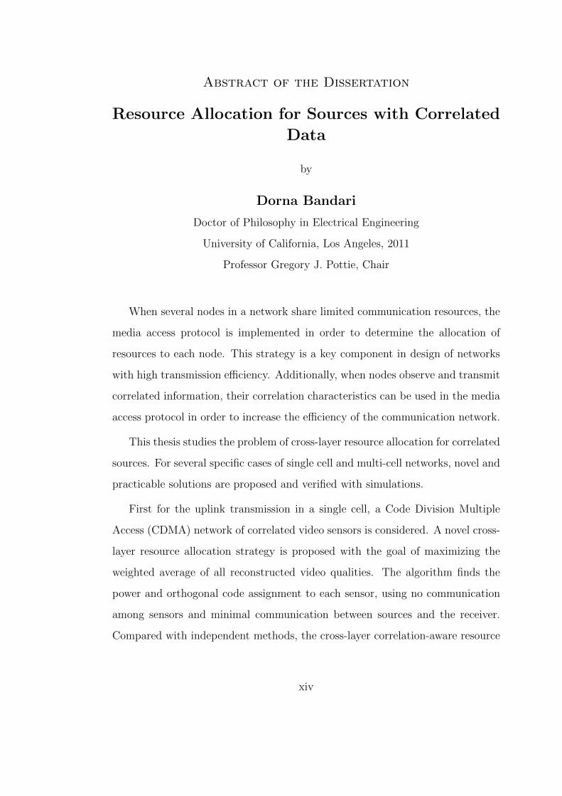
Abstract of the Dissertation

Resource Allocation for Sources with CorrelatedData

by

Dorna Bandari

Doctor of Philosophy in Electrical Engineering

University of California, Los Angeles, 2011

Professor Gregory J. Pottie, Chair

When several nodes in a network share limited communication resources, the

media access protocol is implemented in order to determine the allocation of

resources to each node. This strategy is a key component in design of networks

with high transmission efficiency. Additionally, when nodes observe and transmit

correlated information, their correlation characteristics can be used in the media

access protocol in order to increase the efficiency of the communication network.

This thesis studies the problem of cross-layer resource allocation for correlated

sources. For several specific cases of single cell and multi-cell networks, novel and

practicable solutions are proposed and verified with simulations.

First for the uplink transmission in a single cell, a Code Division Multiple

Access (CDMA) network of correlated video sensors is considered. A novel cross-

layer resource allocation strategy is proposed with the goal of maximizing the

weighted average of all reconstructed video qualities. The algorithm finds the

power and orthogonal code assignment to each sensor, using no communication

among sensors and minimal communication between sources and the receiver.

Compared with independent methods, the cross-layer correlation-aware resource

xiv

allocation achieves significant gain in average sensor video quality.

Secondly, a cross-layer resource allocation strategy is proposed for multi-cell

Orthogonal Frequency Division Multiple Access (OFDMA) networks of general

correlated sources. This method assumes a distance based correlation model

among the sources. The goal is to find the power and orthogonal frequency sub-

band assignment in order to minimize the maximum distortion achieved by any

source in the network. The challenge in this case is to take both the inter-cell

interference and the source correlation characteristics into consideration in the

resource allocation strategy. Our proposed solution solves this large NP-hard

problem in three simple, workable steps.

Additionally, this thesis contributes to the problem of resource allocation

for general multi-cell OFDMA communication networks by introducing a novel

inter-cell interference management scheme, called ICon. This method is based

on concentrating the interference to a cell on a pre-determined frequency band,

which is adapted in order to balance the performance across the network.

xv

CHAPTER 1

Introduction

With high rate wireless communication becoming more commonly used in recent

years, and the rise in the number of devices that share the same wireless medium,

efficient use of system resources is gaining more importance. A key component of

the design of an efficient multi-user system is the multiple access protocol, which

consists of the algorithms and parameters that dictate the allocation of resources

to users. Furthermore, when the system parameters are variable, adaptation in

this resource allocation strategy can achieve significant gain over static methods.

Therefore, it is desired to adaptively allocate resources to the users sharing the

common medium, such that the utility chosen for the system is optimized. The

broad objective of this thesis is to understand and develop algorithms for this

problem in specific system settings.

Figure 1.1: In multi-user networks many users share the common radio resources.

1

This chapter first defines and motivates the specific cases that were studied

in this thesis. Then it lists the contributions and organization of this work.

1.1 Cases Considered

1.1.1 Correlation-aware Design

In some applications, such as Wireless Sensor Networks (WSNs) that measure

temperature, humidity, audio and video, the sources capture and transmit cor-

related information. Correlation can be used in the Presentation layer of OSI

(in coding) in order to increase the coding efficiency. Additionally, coding using

correlation facilitates a trade-off of rates and distortions among the correlated

users, characterized by the rate-distortion (R-D) region. This trade-off can be

used in resource allocation in order to increase the transmission efficiency.

1.1.2 Multi-view Video Systems

Of the applications of correlation-aware resource management, an important one

is resource allocation for multi-view video systems. As an example, an array of

cameras capturing the same scene will have correlated footage, and correlation

characteristics of the captured videos can be used in joint decoding, as well as in

resource allocation when transmitting to a common receiver. The challenges in

this case are to: 1) Assume and verify a model for the rate-distortion region for

lossy joint coding of correlated videos. 2) Perform distributed resource allocation,

since the rate-distortion characteristics of each camera vary in time and cannot

be communicated with the receiver.

2

1.1.3 Cellular Systems

Figure 1.2: Cellular systems.

In recent years, higher data rates have been required from cellular systems,

namely the mobile phone networks, as a result of a surge in mobile web devices.

Multi-cell networks cover large geographical areas in order to ensure continuous

coverage for these devices, and therefore reuse the spectrum at spatially separated

areas. The resource allocation problem in this case should both address the inter-

cell and intra-cell resource management. Inter-cell resource management is the

strategy that determines how the resources are divided among the cells, which

involves interference management, while intra-cell finds the resource allocation

to users in a given cell. The optimal resource allocation in cellular networks

is a large NP-hard problem, and requires heuristics based approximations and

simplifications. We study the general adaptive resource allocation for multi-cell

3

networks, as well as the case with correlated sources.

1.2 Contributions

The objective of this thesis is to study the problem of correlation-aware cross-

layer resource allocation, and to propose practical solutions for this problem in

various network settings. Our main contributions are as follows:

• A novel algorithm for correlation-aware resource allocation for video sen-

sor networks using CDMA is proposed. The proposed end-to-end method

works by using a simple correlated video decoding scheme, and models the

resulting joint R-D function of the sources as a piecewise linear model.

• A novel adaptive interference management scheme is proposed for the uplink

of multi-cell OFDMA networks. The interference to every cell is concen-

trated on a designated frequency band, which is easily adapted in order to

balance the performance across the network.

• An original workable strategy is proposed for resource allocation for sources

with correlated information in multi-cell OFDMA networks, taking into

account both the inter-cell interference and correlation characteristics of

source into account.

1.3 Organization

The remainder of this thesis is organized as follows. Chapter 2 presents some

background technical information required to understand this thesis. Chapter 3

defines the resource allocation problem for multi-view video sources. Our solution

is proposed in Section 3.3 and simulations presented in Section 3.4. Chapter

4

4 presents a solution for inter-cell resource management, namely, ICon. The

solution is described in Section 4.3, and the simulation results are given in Section

4.5. Chapter 5 defines and solves the correlation-aware resource allocation for

multi-cell networks. The solution is described in Section 5.4 and simulations are

presented in Section 5.5. Chapter 6 concludes this thesis.

5

CHAPTER 2

Technical Background

This Chapter presents a number of topics required for understanding this re-

search. We will briefly discuss and provide further references for convex opti-

mization, multiple access protocols, resource allocation, and correlated source

coding.

2.1 Convex Optimization

The significance of convex optimization is in its ability to solve large, practical

engineering problems consistently, using efficient algorithms. In this Section we

provide the general formulation of convex optimization problems, as well as de-

scribe the Lagrange dual decomposition method, appropriate for splitting a large

global optimization problem into locally solvable problems. For further reading

on the subject, please refer to [BV04].

2.1.1 General Formulation

A function, f(x) is convex if its graph lies below the line which joins any two

points of the graph. Figure 2.1 demonstrates a convex function of one variable.

Convex optimization studies the minimization of convex functions over con-

straints also defined by convex functions, i.e. over a convex set. Many communi-

6

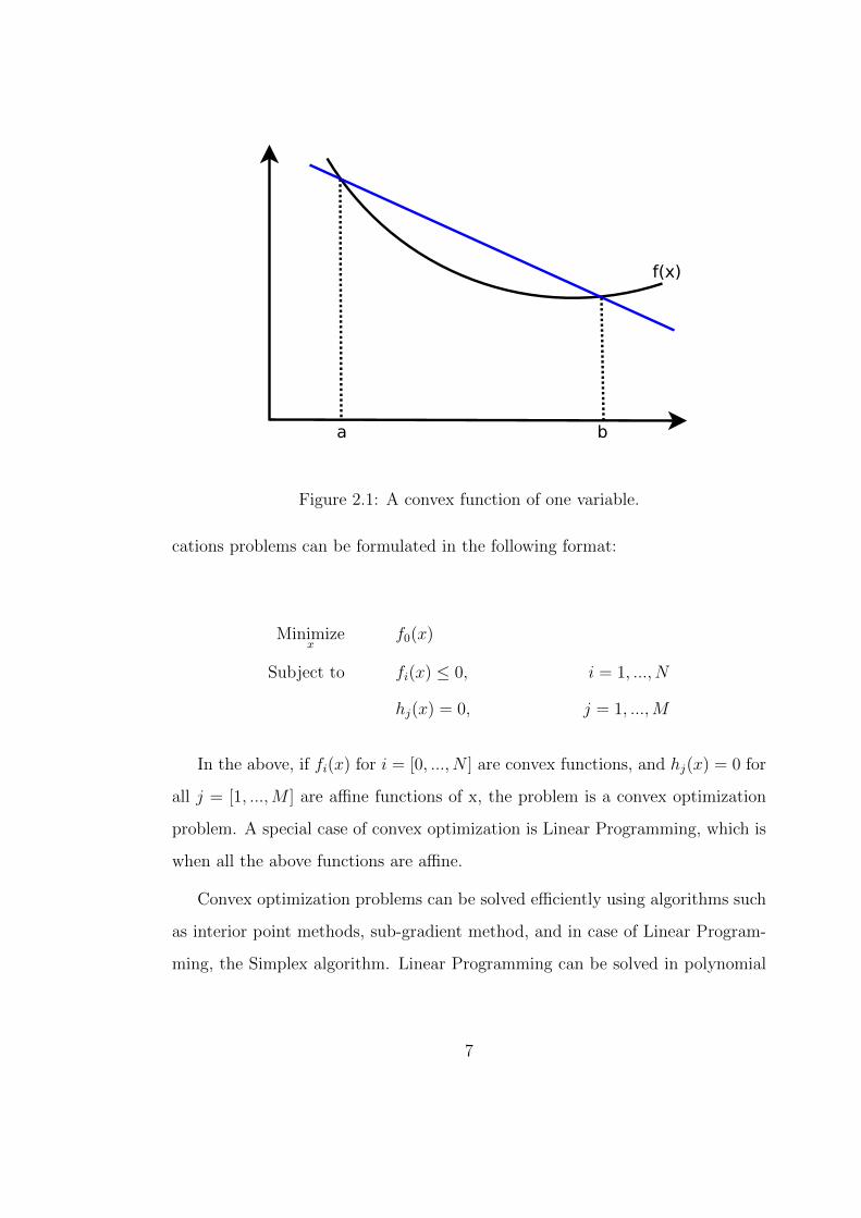
Figure 2.1: A convex function of one variable.

cations problems can be formulated in the following format:

Minimizex

f0(x)

Subject to fi(x) ≤ 0, i = 1, ..., N

hj(x) = 0, j = 1, ...,M

In the above, if fi(x) for i = [0, ..., N ] are convex functions, and hj(x) = 0 for

all j = [1, ...,M ] are affine functions of x, the problem is a convex optimization

problem. A special case of convex optimization is Linear Programming, which is

when all the above functions are affine.

Convex optimization problems can be solved efficiently using algorithms such

as interior point methods, sub-gradient method, and in case of Linear Program-

ming, the Simplex algorithm. Linear Programming can be solved in polynomial

7

time using interior point methods, or in polynomial time average-case using the

Simplex algorithm. Many software packages exist that perform convex optimiza-

tion, we used the CVX package for Matlab [GB11].

2.1.2 Augmented Lagrangian Dual Decomposition Method

In large scale problems it sometimes occurs that the objective function is sepa-

rable and solvable locally by smaller units, e.g. when the objective function is

the sum of utilities of all the units. However some constraints, such as the limits

on total available resources used by the units, couple the local problems. These

constraints prevent the optimization problem from being separable, and solvable

locally by each unit. The Augmented Lagrangian Dual Decomposition method

can be used in such cases in order to enable a distributed solution, requiring

only minimal coordination with a “coordinator” node. For further reading on

the subject, please refer to [PC06].

2.2 Multiple Access Protocols

In multiuser systems, sources share common communication resources. The re-

sources can be shared among the sources in a variety of ways. Namely, they

can be divided along the time (time-division multiple access, TDMA), frequency

(frequency-division multiple access, FDMA), and code (code-division multiple

access, CDMA) axes. In this thesis we have utilized the FDMA and CDMA

methods, and we briefly describe each method in this Section. For further read-

ing on the subject, please refer to [Gol05].

8

2.2.1 CDMA

In order to share the same radio channel, users in a network can modulate their

signal by different spreading codes. The spreading codes can be orthogonal or

non-orthogonal. Orthogonal codes have zero cross-correlation, therefore a receiver

can recover any of the signals by multiplying the received signal by the respective

spreading code. Non-orthogonal codes have non-zero, small cross-correlation. In

this case the receiver recovers the desired signal plus attenuated undesired signals.

In systems with orthogonal CDMA, users do not cause interference to each other

in the network. However they have to be synchronized. Users in systems that

employ non-orthogonal codes on the other hand do not have strict synchronization

requirements, but they cause interference to other users and therefore power

control must be performed in order to limit the interference. In this thesis we

only consider the orthogonal CDMA.

2.2.2 FDMA

In FDMA, users are each assigned a different frequency sub-band from the total

bandwidth. The OFDMA technique implements this by assigning orthogonal

subcarriers to each user. In this case, users do not interfere within the network.

Since users may experience different channel conditions on different sub-bands,

OFDMA can exploit multi-user diversity by enabling channel condition-aware

channel allocation, which is not possible in techniques such as TDMA and CDMA.

2.3 Resource Allocation Problem

In multiuser systems, in addition to selecting an appropriate multiple access pro-

tocol for the given network, the allocation of the resources defined by the multiple

9

access scheme to users should also be found. In resource allocation problems the

issue is the assignment of limited communication resources to users. In this chap-

ter we discuss the general formulation of the resource allocation problem and the

case for multi-cell systems. For further reading on the subject, please refer to

[ZQ01].

2.3.1 General Formulation

The aim of resource allocation is to assign limited communication resources to

users, such that a pre-defined utility is maximized in the network. When chan-

nel conditions or transmission requirements of users change in time, the resource

allocation must be performed adaptively. First, an appropriate utility function

should be chosen for the system, and the relationship between the resource as-

signment to users and network utility should be derived. Given this relationship,

the resources must be assigned such that the utility is optimized.

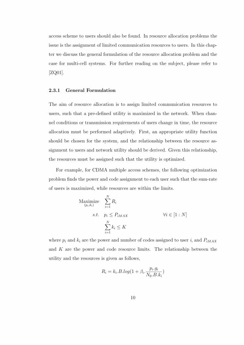
For example, for CDMA multiple access schemes, the following optimization

problem finds the power and code assignment to each user such that the sum-rate

of users is maximized, while resources are within the limits.

Maximize(pi,ki)

N�

i=1

Ri

s.t. pi ≤ PiMAX ∀i ∈ [1 : N ]

N�

i=1

ki ≤ K

where pi and ki are the power and number of codes assigned to user i, and PiMAX

and K are the power and code resource limits. The relationship between the

utility and the resources is given as follows,

Ri = ki.B.log(1 + βi.pi.gi

N0.B.ki)

10

where B is the total available bandwidth and βi is the SNR gap, which accounts

for the difference between the theoretical achievable rate and the achievable rate

in a real system. gi is the channel gain for user i, and N0 is the noise floor.

2.3.2 Multi-cell systems

In order to cover a large geographic area efficiently, infrastructure-based wireless

networks can be divided into cells, each cell containing a base-station which is con-

nected to the backbone wired network. This enables efficient use of resources by

reusing frequency spectrum in geographically separated areas. However, the re-

source allocation task thus becomes more complicated, since orthogonal resource

allocation across the whole network is no longer possible or efficient. Inter-cell

interference management addresses the issue of resource allocation among inter-

fering cells, and is part of the resource allocation problem for multi-cell systems.

2.4 Correlated Sources

When sources gather and aim to transmit correlated information, correlation

should be used in both the coding and resource allocation in order to increase

the efficiency of the system. This occurs in wireless sensor networks (WSNs)

where sensors on a field measure various parameters such as temperature, hu-

midity, audio or video. In this work we have considered an array of video sensors

capturing the same scene from different angles, as well as general WSNs. In this

section we discuss the joint coding basics and the rate-distortion region.

11

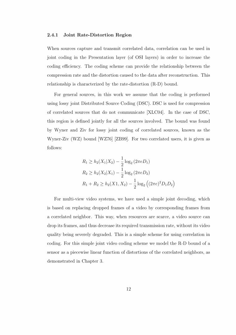
2.4.1 Joint Rate-Distortion Region

When sources capture and transmit correlated data, correlation can be used in

joint coding in the Presentation layer (of OSI layers) in order to increase the

coding efficiency. The coding scheme can provide the relationship between the

compression rate and the distortion caused to the data after reconstruction. This

relationship is characterized by the rate-distortion (R-D) bound.

For general sources, in this work we assume that the coding is performed

using lossy joint Distributed Source Coding (DSC). DSC is used for compression

of correlated sources that do not communicate [XLC04]. In the case of DSC,

this region is defined jointly for all the sources involved. The bound was found

by Wyner and Ziv for lossy joint coding of correlated sources, known as the

Wyner-Ziv (WZ) bound [WZ76] [ZB99]. For two correlated users, it is given as

follows:

R1 ≥ h2(X1|X2)−1

2log2 (2πeD1)

R2 ≥ h2(X2|X1)−1

2log2 (2πeD2)

R1 +R2 ≥ h2(X1, X2)−1

2log2

�(2πe)2D1D2

�

For multi-view video systems, we have used a simple joint decoding, which

is based on replacing dropped frames of a video by corresponding frames from

a correlated neighbor. This way, when resources are scarce, a video source can

drop its frames, and thus decrease its required transmission rate, without its video

quality being severely degraded. This is a simple scheme for using correlation in

coding. For this simple joint video coding scheme we model the R-D bound of a

sensor as a piecewise linear function of distortions of the correlated neighbors, as

demonstrated in Chapter 3.

12

CHAPTER 3

Correlation used in resource allocation for

single-cell networks

3.1 Introduction

In this chapter we consider a scenario where several cameras capture a live event

and stream it simultaneously to a base station. The applications are live coverage

of concerts, conferences, or political events. With free-view and multi-view video

becoming more popular, and with limited resources in wireless transmission, we

expect an increased demand for more efficient streaming of correlated videos.

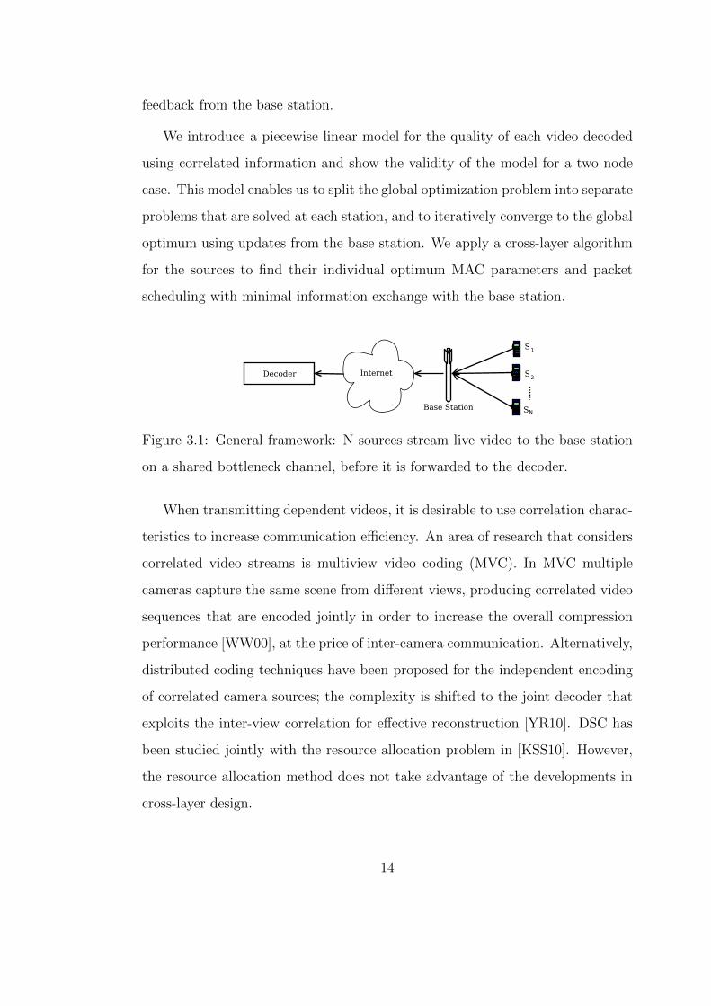
We consider the scenario of N video sources transmitting correlated video

streams through a shared wireless channel to a common base station, before

delivery to the decoder. In this work we consider a regular H.264 video encoder

and a simple decoder which uses correlation between sources for concealment of

missing frames. The goal is to maximize the weighted sum of received video

qualities given the resource constraints. The decoder may use source correlation

to decode the N videos in case of insufficient bandwidth or loss, as shown in

Figure 3.1. We consider Code Division Multiple Access (CDMA) as the MAC

scheme, however the methods developed in this paper can be applied to other

access schemes. We formulate an optimization problem that selects the best code,

power assignment, and packet selection at each wireless source, with minimal

13

feedback from the base station.

We introduce a piecewise linear model for the quality of each video decoded

using correlated information and show the validity of the model for a two node

case. This model enables us to split the global optimization problem into separate

problems that are solved at each station, and to iteratively converge to the global

optimum using updates from the base station. We apply a cross-layer algorithm

for the sources to find their individual optimum MAC parameters and packet

scheduling with minimal information exchange with the base station.

Figure 3.1: General framework: N sources stream live video to the base station

on a shared bottleneck channel, before it is forwarded to the decoder.

When transmitting dependent videos, it is desirable to use correlation charac-

teristics to increase communication efficiency. An area of research that considers

correlated video streams is multiview video coding (MVC). In MVC multiple

cameras capture the same scene from different views, producing correlated video

sequences that are encoded jointly in order to increase the overall compression

performance [WW00], at the price of inter-camera communication. Alternatively,

distributed coding techniques have been proposed for the independent encoding

of correlated camera sources; the complexity is shifted to the joint decoder that

exploits the inter-view correlation for effective reconstruction [YR10]. DSC has

been studied jointly with the resource allocation problem in [KSS10]. However,

the resource allocation method does not take advantage of the developments in

cross-layer design.

14

In general, the wireless resource allocation for correlated video sources has not

been studied extensively in the literature. In the area of multimedia communica-

tion for independent sources, it has been thoroughly demonstrated that there is

significant benefit in using cross-layer design as compared to traditional layered

design for live video transmissions [SRK03] [DN05]. The works in [SBA10] and

[SL05] propose optimal solutions for a utility-based cross-layer resource alloca-

tion. These methods however consider downlink communications, which does not

present the same challenges as uplink, in particular the fact that each sources’

individual constraints (e.g., power) also needs to be considered.

Among uplink optimum resource allocation solutions, the following three pa-

pers are most related to our work. In [HSB07] an uplink OFDM system is consid-

ered and a utility-based objective function is optimized, although not specific to

video sources. In [SS08] optimal resource allocation is performed for uplink trans-

mission of video sources; specifically algorithms are developed to assign MAC re-

sources to each video source in a centralized manner, optimizing overal received

quality. In [Cha06] optimum rate allocation and packet scheduling for video

sources is found for uplink tranmission, with the objective of maximizing the

overall video quality. However the individual MAC parameters are not found,

which does not allow for adaptation to changes in availability of individual re-

sources. None of the works explicitly consider the sources’ correlation in the rate

allocation problem.

The rest of the sections of this chapter are as follows. In Section 3.2 we

introduce the framework of our proposed method and formulate the problem.

In Section 3.3 we discuss the piecewise linear model and give details on the

optimization solution. In Section 3.4 we present simulations for validation of the

piecewise linear quality model, as well as overall resource allocation results.

15

3.2 Problem Settings

3.2.1 Framework

We consider the transmission of N correlated video sources through one com-

mon base station. We consider that the sources have no possibility to precisely

adapt the video encoding to the actual transmission conditions, so that the rate

allocation problem becomes equivalent to a packet scheduling optimization. A

joint decoder reconstructs each of the views. It uses the inter-view correlation

information to compensate missing information due to frames that have been lost

or dropped. We consider here a very simple concealment strategy where miss-

ing frames are replaced by the corresponding data in the most correlated views.

Note that the error concealment can be chosen differently without affecting the

resource allocation framework proposed in this chapter.

Our objective is to maximize the weighted sum of qualities of all received

videos. In case of concealment we model the quality of each video as the weighted

sum of qualities of its neighbours, where the weights depend on video character-

istics, correlation between sources, and packet loss probability. Then the global

optimization problem is split into local optimization problems solved at each

source, and the global optimum is reached iteratively by using updates from the

base station. As we choose CDMA as the Multiple Access scheme, the variables

to be found are the optimum code and power assignment and packet scheduling

for each individual source.

3.2.2 Problem Formulation

First, we note that the transmission rate can be written as a function of the MAC

parameters. In a Gaussian multiple-access channel, the achievable rate for user i

16

in terms of CDMA parameters is given by [Gol05],

Ri = ki.B.log(1 + ζi.piki), (3.1)

where pi is the power allocated to user i and ki is the number of orthogonal

codes assigned to it. B is the total available bandwidth, and ζi = βi

gi

N0.B. The

parameter βi is called the SNR gap, which accounts for the difference between

the theoretical achievable rate and the achievable rate in a real system. gi is the

channel gain for user i, and N0 is the noise floor. We name N0.B

githe Normalized

Noise for user i.

The resource allocation problem consists in finding the optimal code choice,

power assignment and packet selection at each of the CDMA sources, so that the

overall quality is maximized. The problem can be formulated as follows.

Minimize(pi,ki)

−QT (R) (3.2)

s.t. pi ≤ PiMAX ∀i ∈ [1 : N ]

N�

i=1

ki ≤ K

N�

i=1

pi ≤ PT

QT (R) represents the objective function, with the aggregate decoding quality. It

is a function of R, the vector of rates of each source as given by Eq (5.1). PiMAX

is the maximum power for source i, K is the total number of available codes, and

PT is the total power that can be used by the network. In the next section we

propose a solution to optimize this problem with a simple iterative algorithm.

17

3.3 Optimal Resource Allocation

3.3.1 Aggregate Utility Model

In general, the quality of a decoded video stream, when decoded using correlation

irrespective of the decoding scheme, is a function of its own data rate as well as

data rates of videos that are correlated to it. When the rates are denoted by the

vector R, the quality of video i becomes

Qc

i(R) = f(R1, R2, R3, ...) (3.3)

A concave, monotonically increasing quality-rate function can be constructed

for any video stream. When the stream is pre-encoded, rate adaptation can be

achieved by packet filtering. A packet ordering algorithm such as one proposed

in [CF05] can be used to order the frames so that the least important packets are

dropped first when resources become scarce.

That being said, our resource allocation method does not require all nodes to

order their frames, and if complexity is strictly constrained, each node can choose

to use a known model for its Q-R function. Of course, using a model results

in a sub-optimal solution. One such function is given in [SFL00]. Whether a

known model is used or an optimum algorithm utilized, the resulting quality-rate

function is bijective. Therefore we can replace the rate in equation (3.3) by the

quality from the estimated Q-R function, formulating the decoding quality as a

function of quality of the correlated video sequences, i.e.,

Qc

i(R) = f(Q1(R1), Q2(R2), Q3(R3), ...)

We now propose a simple piecewise first order approximation of the above func-

18

tion in the decoder, with a linear combination of qualities:

Qc

i(R) =

N�

j=1

αm

ij.Qj(Rj) + δm

i, Q

N∈ CN

m. (3.4)

QN

is the array of quality-rate functions, i.e. [Q1(R1)...-QN(RN)]. The model

parameters, αm

ijs and δm

is are estimated for the range of values of Q

Nthat belong

to the N dimensional space CN

m. In this work CN

ms are constructed by partitioning

the range of possible values for qualities of each video into 2dB sections. Therefore

any value for the array of qualities, QN, belongs to one such space.

The model parameters are initially calculated at the decoder by decoding

videos in two ways; regular decoding, which results in videos with qualities QN,

and correlated decoding, which is used to find values for Qc

i(R)s. Then, for each

range of video quality values, CN

m, the model parameters, αm and δm, are found

by fitting the video quality values to the model from Equation (3.4), using LMS.

Depending on the correlation level and the qualities of the correlated videos,

it is possible for the correlated decoding method to decrease the quality of a

decoded video when compared to regular decoding, i.e., for some i and some m,

Qc

i(R) < Qi(Ri), Q

N∈ CN

m.

To ensure that we always decode using the method that achieves the higher

decoded quality, the decoder can simply set the model parameters to a row of

the identity matrix in such cases.

ifN�

j=1

αm

ij.Qj(Rj) + δm

i< Qi(Ri), set

αm

ii= 1,

αm

ij= 0, ∀j �= i

δmi= 0.

19

The aggregate quality of the network finally becomes

QT (R) =N�

i=1

γi.Qc

i(R)

=N�

j=1

�N�

i=1

γi.αm

ij.Qj(Rj)

�

+N�

i=1

δmi.γi

=N�

j=1

ηj.Qj(Rj) + δmj.γj, (3.5)

where ηj =�

N

i=1 γi.αm

ijand γi is a parameter set by network administrators as

a measure of relative importance of each video stream in the aggregate quality

function. It can be shown that the above is a concave function of pi and ki [BV04],

which makes (3.2) a convex optimization problem with linear constraints.

3.3.2 Optimization Solution

In order to solve the optimization problem presented in Section 5.3 we first formu-

late it as an unconstrained optimization problem. The Lagrangian cost function

is given by

L(k,p,λ, ν,ω) = −QT (R) + λ.[p− PMAX ]T + ν.(N�

i=1

ki −K) + ω.(N�

i=1

pi − PT ),

where λ = [λ1λ2...λN ], ν and ω are the dual variables, p = [p1, p2, ..., pN ] is the

vector of power assignments, k = [k1, k2, ..., kN ] is the vector of number of codes

assigned to each user, and PMAX = [P1MAX , P2MAX , ..., PNMAX ]T is the vector of

power limits of each user. K is the total number of codes, and PT is the maximum

total power allowed in the network. Then taking the infimum over k and p will

result in the Lagrange dual function,

g(λ, ν,ω) = infk,p

(L(k,p,λ, ν,ω))

In this problem strong duality holds, therefore solving the Lagrange dual

function will solve the primal problem. To solve the unconstrained concave dual

20

problem, the partial derivatives of Lagrangian function with respect to p and k

are set to zero. For each station we get the following two equations,

B.ηi.

�

log(1 + ζi.piki)− pi.ζi

(ki + pi.ζi). ln(10)

�

.dQ(i)(Ri)

dRi

= ν (3.6)

B.ηi.ζiln(10)

.[ki

ki + pi.ζi].dQ(i)(Ri)

dRi

= λi + ω (3.7)

Once the above two equations are solved for pi and ki in each station, the dual op-

timal variables can be found iteratively using the sub-gradient method. Starting

from λ0,ω0, ν0, repeat,

λk+1i

= (λk

i+ θ.(p∗

i− PiMAX))

+ (3.8)

νk+1 = (νk + δ.(N�

i=1

k∗i−K))+ (3.9)

ωk+1 = (ωk + ε.(N�

i=1

p∗i− PT ))

+. (3.10)

θ, δ, and ε are small constants, and (x)+ is 0 for x ≤ 0 and x otherwise. Since

source nodes do not have access to information about other stations’ power and

code assignment, the variables νk+1 and ωk+1 have to be computed at the base

station or the receiver. Their value is periodically broadcasted back to the sta-

tions. Algorithm 1 describes this method.

At each source, the system of equations, (3.6) and (3.7) is solved by defining

a new variable, Xi = (1 + pi

ki.ζi), and dividing the two equations in order to

eliminate dQ(i)(Ri)dRi

. After rearranging, we get the following:

Xi.(log(Xi)−1

ln 10) =

ν.ζi(λi + ω). ln 10

− 1

ln 10. (3.11)

There is always a unique solution for Xi. This can be solved by a simple table

look up at each source. Once Xi is found, each station finds its own optimum

21

Algorithm 1: Optimal Resource Allocation

Input: Constraints: K,PT ,PMAX ; Channel parameters: B,η, ζ; CN

ms found

by 2dB partitions of video quality values.

Initialization: ν0 = ω0 = 0.5,λ0i= 0.5 ∀i, k = 0, flag = 0,αn =

IN×N ∀n, andm = 0.

Repeat:

At each source, i:

1) Capture and encode Wk video frames.

2) Arrange frames in the order of contribution to video quality, or assume

a model for the Q-R plot, as in Section 3.3.1.

3) Using νk,ωk and λk

ifind p∗

i, k∗

iand optionally the optimum set of

frames to transmit by solving Equations (3.11) through (3.13).

4) Transmit the optimum set of frames using MAC parameters, p∗i, k∗

i.

5) Update λk+1i

using Equation (3.8).

At base station:

6) Receive video frames from all sources, forward to the decoder.

7) Find νk+1 and ωk+1 using (3.9) and (3.10).

8) Broadcast νk+1 and ωk+1, and if flag = 1, αm.

At the decoder:

In the initial phase: Find αm parameters using method described in

Section 3.3.1.

Otherwise:

9) Using the rate vector, [R1...RN ], calculate the quality vector,

[Q1(R1), ...QN(RN)].

10) Find m� such that [Q1(R1), ...QN(RN)] ∈ CN

m� . If m� �= m, then m = m�

and flag = 1.

11) Decode the videos, with error concealment method depending on values

of αm.

22

dQ(i)(Ri)dRi

using Equation (3.7). Then, using its corresponding Q-R function, the

station finds the rate at which the slope of Q-R plot matches the found dQ(i)(Ri)dRi

,

which is its optimum rate, Ri. If a packet ordering algorithm was used to create

the Q-R function, the station also simultaneously finds its packet selection. The

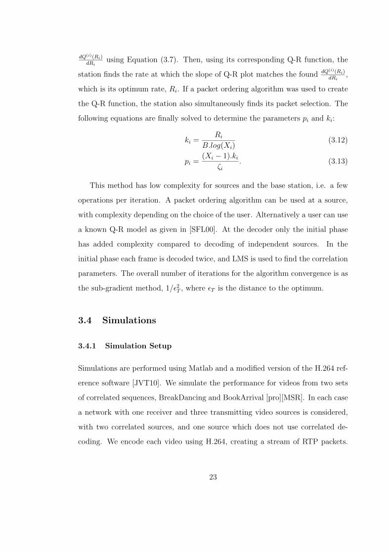
following equations are finally solved to determine the parameters pi and ki:

ki =Ri

B.log(Xi)(3.12)

pi =(Xi − 1).ki

ζi. (3.13)

This method has low complexity for sources and the base station, i.e. a few

operations per iteration. A packet ordering algorithm can be used at a source,

with complexity depending on the choice of the user. Alternatively a user can use

a known Q-R model as given in [SFL00]. At the decoder only the initial phase

has added complexity compared to decoding of independent sources. In the

initial phase each frame is decoded twice, and LMS is used to find the correlation

parameters. The overall number of iterations for the algorithm convergence is as

the sub-gradient method, 1/�2T, where �T is the distance to the optimum.

3.4 Simulations

3.4.1 Simulation Setup

Simulations are performed using Matlab and a modified version of the H.264 ref-

erence software [JVT10]. We simulate the performance for videos from two sets

of correlated sequences, BreakDancing and BookArrival [pro][MSR]. In each case

a network with one receiver and three transmitting video sources is considered,

with two correlated sources, and one source which does not use correlated de-

coding. We encode each video using H.264, creating a stream of RTP packets.

23

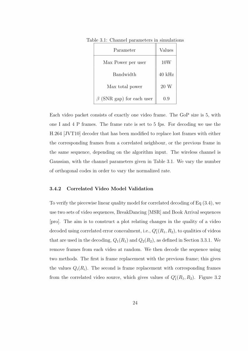
Table 3.1: Channel parameters in simulations

Parameter Values

Max Power per user 10W

Bandwidth 40 kHz

Max total power 20 W

β (SNR gap) for each user 0.9

Each video packet consists of exactly one video frame. The GoP size is 5, with

one I and 4 P frames. The frame rate is set to 5 fps. For decoding we use the

H.264 [JVT10] decoder that has been modified to replace lost frames with either

the corresponding frames from a correlated neighbour, or the previous frame in

the same sequence, depending on the algorithm input. The wireless channel is

Gaussian, with the channel parameters given in Table 3.1. We vary the number

of orthogonal codes in order to vary the normalized rate.

3.4.2 Correlated Video Model Validation

To verify the piecewise linear quality model for correlated decoding of Eq (3.4), we

use two sets of video sequences, BreakDancing [MSR] and Book Arrival sequences

[pro]. The aim is to construct a plot relating changes in the quality of a video

decoded using correlated error concealment, i.e., Qc

1(R1, R2), to qualities of videos

that are used in the decoding, Q1(R1) and Q2(R2), as defined in Section 3.3.1. We

remove frames from each video at random. We then decode the sequence using

two methods. The first is frame replacement with the previous frame; this gives

the values Qi(Ri). The second is frame replacement with corresponding frames

from the correlated video source, which gives values of Qc

1(R1, R2). Figure 3.2

24

25

30

35

4045

25

30

35

40

4526

28

30

32

34

36

38

40

42

Y−PSNR Video 2Y−PSNR Video 1

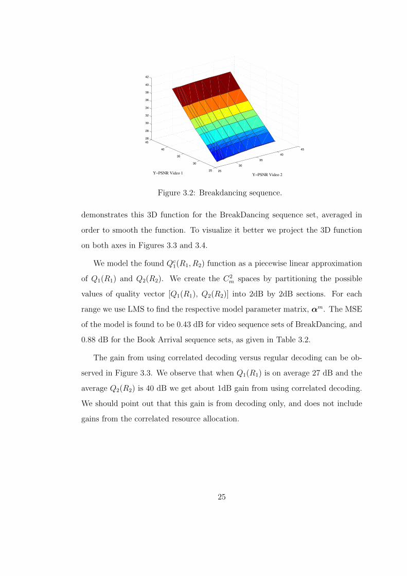
Figure 3.2: Breakdancing sequence.

demonstrates this 3D function for the BreakDancing sequence set, averaged in

order to smooth the function. To visualize it better we project the 3D function

on both axes in Figures 3.3 and 3.4.

We model the found Qc

1(R1, R2) function as a piecewise linear approximation

of Q1(R1) and Q2(R2). We create the C2m

spaces by partitioning the possible

values of quality vector [Q1(R1), Q2(R2)] into 2dB by 2dB sections. For each

range we use LMS to find the respective model parameter matrix, αm. The MSE

of the model is found to be 0.43 dB for video sequence sets of BreakDancing, and

0.88 dB for the Book Arrival sequence sets, as given in Table 3.2.

The gain from using correlated decoding versus regular decoding can be ob-

served in Figure 3.3. We observe that when Q1(R1) is on average 27 dB and the

average Q2(R2) is 40 dB we get about 1dB gain from using correlated decoding.

We should point out that this gain is from decoding only, and does not include

gains from the correlated resource allocation.

25

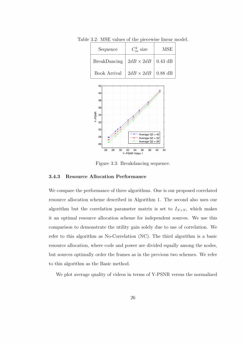
Table 3.2: MSE values of the piecewise linear model.

Sequence C2msize MSE

BreakDancing 2dB × 2dB 0.43 dB

Book Arrival 2dB × 2dB 0.88 dB

26 28 30 32 34 36 38 40 42

26

28

30

32

34

36

38

40

42

Y−PSNR Video 1

Y−PS

NR

Average Q2 = 40Average Q2 = 32Average Q2 = 26

Figure 3.3: Breakdancing sequence.

3.4.3 Resource Allocation Performance

We compare the performance of three algorithms. One is our proposed correlated

resource allocation scheme described in Algorithm 1. The second also uses our

algorithm but the correlation parameter matrix is set to IN×N , which makes

it an optimal resource allocation scheme for independent sources. We use this

comparison to demonstrate the utility gain solely due to use of correlation. We

refer to this algorithm as No-Correlation (NC). The third algorithm is a basic

resource allocation, where code and power are divided equally among the nodes,

but sources optimally order the frames as in the previous two schemes. We refer

to this algorithm as the Basic method.

We plot average quality of videos in terms of Y-PSNR versus the normalized

26

26 28 30 32 34 36 38 40 42

26

28

30

32

34

36

38

40

42

Y−PSNR Video 2

Y−PS

NR

Average Q1 = 40Average Q1 = 32Average Q1 = 26

Figure 3.4: Breakdancing sequence.

rate. The normalized rate is calculated by dividing the total load by the channel

capacity. We consider two cases for channel conditions. In the first case the two

correlated sources experience 23 and 17 dBm Normalized Noise, as defined in

Eq. 5.1, and the uncorrelated source has normalized noise of of 23 dBm. The

resulting performance for each video sequence set is given in Figures 3.5(a) and

3.5(b). We observe that the proposed algorithm has up to 0.5 dB higher average

Y-PSNR than the NC method for the BreakDancing sequences, and at worst case

it performs equally well. For the BookArrival sequence our proposed method has

the same performance as the NC.

We then consider the normalized noise of 27 dBm and 17 dBm for the corre-

lated sources and 20 dBm for the independent source. The results are presented

in Figures 3.6(a) and 3.6(b). In this case for both videos we see gain, up to

1.75 dB in average video quality, in our proposed method compared with the

NC method. The basic method performs poorly since the quality found for the

user with the worst channel drops to zero when normalized rate is at 0.87 for

BreakDancing and at 1 for BookArrival sequence sets.

27

0.65 0.7 0.75 0.8 0.85 0.9 0.95 1 1.05 1.136

37

38

39

40

41

42

43

44

Normalized Rate

Ave

rage

Qua

lity

NCBasicProposed

(a) BreakDancing

0.6 0.7 0.8 0.9 1 1.131

32

33

34

35

36

37

38

39

Normalized Rate

Ave

rage

Qua

lity

NCBasicProposed

(b) BookArrival

Figure 3.5: Average quality for 3 sources, Normalized Noise power (dBm) = [23,

17, 23].

0.65 0.7 0.75 0.8 0.85 0.9 0.95 1 1.05 1.126

28

30

32

34

36

38

40

42

44

Normalized Rate

Ave

rage

Qua

lity

NCBasicProposed

(a) BreakDancing

0.65 0.7 0.75 0.8 0.85 0.9 0.95 1 1.05 1.124

26

28

30

32

34

36

38

Normalized Rate

Ave

rage

Qua

lity

NCBasicProposed

(b) BookArrival

Figure 3.6: Average quality for 3 sources, Normalized Noise power (dBm) = [27,

17, 20].

3.5 Conclusion

In this chapter we propose a method to find the optimum resource allocation for

uplink transmission of correlated video sources, such that the total received video

quality is maximized. We develop a model for relating the quality of a video de-

28

coded using correlation to quality-rate characteristic functions of videos that are

used in its decoding. Based on this model, we formulate an optimization problem

and develop an algorithm to solve it with little information exchange with the

base station. From the simulations we observe that even with a simple corre-

lated error concealment scheme, our proposed resource allocation method results

in up to 1.75 dB gain over the optimum resource allocation with independent

decoding, which provides a lower-bound on the performance of our algorithm.

The small additional complexity at the decoder resides in the estimation of the

source correlation parameters, which is generally only performed once in a static

setting.

29

CHAPTER 4

ICon: Multi-cell OFDMA based resource

allocation using interference concentration

4.1 Introduction

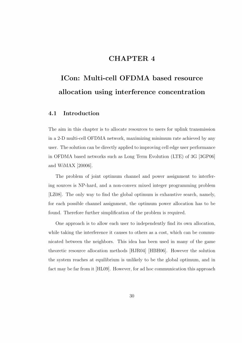
The aim in this chapter is to allocate resources to users for uplink transmission

in a 2-D multi-cell OFDMA network, maximizing minimum rate achieved by any

user. The solution can be directly applied to improving cell edge user performance

in OFDMA based networks such as Long Term Evolution (LTE) of 3G [3GP06]

and WiMAX [20006].

The problem of joint optimum channel and power assignment to interfer-

ing sources is NP-hard, and a non-convex mixed integer programming problem

[LZ08]. The only way to find the global optimum is exhaustive search, namely,

for each possible channel assignment, the optimum power allocation has to be

found. Therefore further simplification of the problem is required.

One approach is to allow each user to independently find its own allocation,

while taking the interference it causes to others as a cost, which can be commu-

nicated between the neighbors. This idea has been used in many of the game

theoretic resource allocation methods [HJR04] [HBH06]. However the solution

the system reaches at equilibrium is unlikely to be the global optimum, and in

fact may be far from it [HL09]. However, for ad hoc communication this approach

30

might be the only option.

When the network has a known, fixed structure however, a better approach

is to exploit this knowledge in order to simplify the problem. For example,

for cellular networks this approach will be as follows. A predetermined Inter-

Cell Interference Coordination (ICIC) rule can be found for the given network

parameters, i.e., cell size, transmit powers, cell load, etc. The ICIC determines

the inter-cell resource management [3GP06]. Then each cell can independently

schedule its users, for example using frame by frame Proportionally Fair (PF)

scheduling [WOG05], while following the inter-cell interference rules.

In this chapter we are proposing a two phase solution: the ICIC adaptation

phase (i.e. Interference Concentration (ICon)) and intra-cell scheduling phase.

At each iteration of ICon, inter-cell resource management is found, given the

performance achieved in each cell in the previous iteration. Then, having fixed

the inter-cell resource management, the intra-cell scheduling problem becomes a

linear programming problem for which fast and simple solutions exist[BV04].

The idea behind the two phase approach is that when the inter-cell resource

management rule is found and optimized using communication theory and ex-

periments, the solution space of the original NP-hard problem is limited to the

most reasonable options. And although global optimality is not guaranteed in

this method either, it greatly reduces the problem size and complexity.

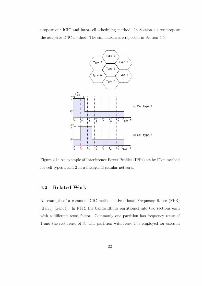
• We first propose ICon, a novel inter-cell resource management method based

on defining Interference Power Profiles (IPPs) for cells. The IPP defines

a limit to received interference on each sub-band, which the neighboring

cells are obliged to meet. An example is given in Figure 5.4. The idea

is that if the high interference causing users from all neighboring cells are

concentrated on the same band, the bandwidth will be used more efficiently.

31

• In order to balance performance across cells, ICon is made adaptable. At

each ICIC adaptation time, cells broadcast the average utility they achieved

in the previous period (e.g. over the X2 interface in LTE). Then each cell

updates the IPP it imposes on its neighbors, given its performance relative

to theirs. Each cell loosens its IPP requirements for neighbors that have

worse performance than itself, and tightens it for neighbors that perform

better.

• In the Intra-cell scheduling phase each cell finds the transmit power limits

for each user on each sub-band such that none of its neighbors’ IPPs is

violated. This is easily done using channel gains between each user and

the neighboring base stations (BSs), which is available at each user given

pilots from neighboring BSs, assuming channel reciprocity holds (available

in LTE for use in hand-off). Once the maximum transmit powers are found

for each user on each sub-band, a linear optimization problem can be solved

by each base station in order to allocate channels to its users, maximizing

the minimum rate in the cell. This can be updated frequently since linear

optimization problems are efficiently solved.

Our contributions in this chapter are twofold. First is that we propose a

novel inter-cell interference management scheme based on interference concen-

tration (i.e. ICon). ICon outperforms the common ICIC methods in cell edge

user performance, it is simple to implement, easily adaptable, and can be applied

to all OFDMA-based networks. Secondly, we combine ICon with inter-cell re-

source optimization and propose a two phase solution that adaptively improves

the global performance of the network.

The rest of the chapter is as follows. Related work will be presented in Section

4.2. We define the optimization problem we aim to solve in Section 4.3 and

32

propose our ICIC and intra-cell scheduling method. In Section 4.4 we propose

the adaptive ICIC method. The simulations are reported in Section 4.5.

Figure 4.1: An example of Interference Power Profiles (IPPs) set by ICon method

for cell types 1 and 2 in a hexagonal cellular network.

4.2 Related Work

An example of a common ICIC method is Fractional Frequency Reuse (FFR)

[Hal83] [Gen04]. In FFR, the bandwidth is partitioned into two sections each

with a different reuse factor. Commonly one partition has frequency reuse of

1 and the rest reuse of 3. The partition with reuse 1 is employed for users in

33

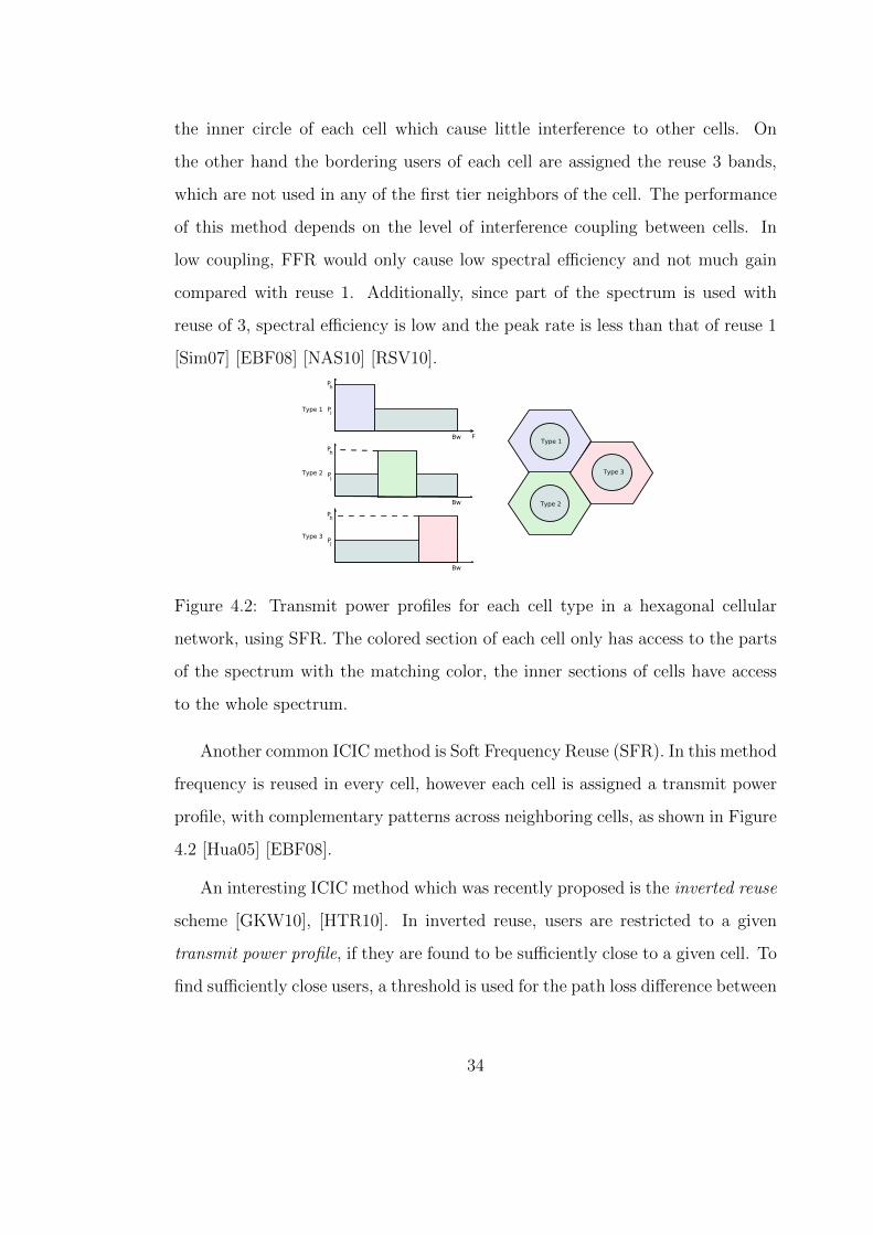
the inner circle of each cell which cause little interference to other cells. On

the other hand the bordering users of each cell are assigned the reuse 3 bands,

which are not used in any of the first tier neighbors of the cell. The performance

of this method depends on the level of interference coupling between cells. In

low coupling, FFR would only cause low spectral efficiency and not much gain

compared with reuse 1. Additionally, since part of the spectrum is used with

reuse of 3, spectral efficiency is low and the peak rate is less than that of reuse 1

[Sim07] [EBF08] [NAS10] [RSV10].

Figure 4.2: Transmit power profiles for each cell type in a hexagonal cellular

network, using SFR. The colored section of each cell only has access to the parts

of the spectrum with the matching color, the inner sections of cells have access

to the whole spectrum.

Another common ICIC method is Soft Frequency Reuse (SFR). In this method

frequency is reused in every cell, however each cell is assigned a transmit power

profile, with complementary patterns across neighboring cells, as shown in Figure

4.2 [Hua05] [EBF08].

An interesting ICIC method which was recently proposed is the inverted reuse

scheme [GKW10], [HTR10]. In inverted reuse, users are restricted to a given

transmit power profile, if they are found to be sufficiently close to a given cell. To

find sufficiently close users, a threshold is used for the path loss difference between

34

the serving BS and the neighboring BS. Since all users in all cells neighboring

a cell will be given the same power profile, the received interference at the cell

will be concentrated as given by that power profile. Our proposed ICIC scheme

uses a similar idea as the inverted reuse, that is to shape the interference of a

cell. However, we directly define an interference power profile (IPP) for each cell

which allows for more direct and intuitive adaptation.

The work in [FSC10] also uses the idea of assigning interference profiles for

uplink ICIC using Overload Indicators (OIs) defined by 3gpp for LTE of 3G.

Fixed interference profiles similar to transmit power profiles in SFR are assigned

to cells. This work requires each cell to identify the high interference users in the

nearby cells, and therefore requires more processing and inter-cell communication.

For inter-cell resource allocation, Proportionally Fair (PF) scheduling is a

common method for LTE. This method is simple to implement and can be mod-

ified to achieve different levels of fairness [WOG05]. Additionally for single cell

OFDM networks, the optimal allocation of power per subband per user is found

to be a convex optimization problem [LZ08], solvable in polynomial time.

4.3 Optimization Problem

We consider a 2-D multi-cell network with OFDMAmultiple access scheme. Users

in each cell are allocated resources by the scheduler located in the cell base

station for uplink communication. The resources to assign are power and channel

allocation to each user. Each of the independent orthogonal channels are assumed

to be Gaussian and interference is considered to be equivalent to noise in terms

of channel capacity. The variables to find are each user’s transmit power spectral

density for each channel, pi,c and channel assignment, ai,c which is a binary array.

35

We assume no intra cell interference. The following rate is achieved for user i in

cell k :

Ri,k =C�

c=1

ai,c.Bc. log2

�

1 +pi,c.gik

N0.Bc +�

K

u=1,u �=kP I

ukc

�

, (4.1)

where gik is the channel gain from user i to receiver of cell k, Bc is the bandwidth

of channel c. N0 is the noise power and P I

ukcis the received interference power

from cell u to cell k on channel c. Namely, P I

ukc=

�j∈Xu

aj,c.pj,c.gjk.

Maximizea,p

mini,k

(Ri,k) (4.2)

�

i∈kai,c = 1, ai,c ∈ {0, 1} ∀k

PMIN ≤ pi,k ≤ PMAX , ∀i, k

where Ri,k is given as Eq. (5.1). This problem is NP-hard for (C > 1) [LZ08].

NP hardness of (4.2) means that optimality of any solution cannot be guaran-

teed unless with exhaustive search over all possible solutions. Therefore we can

only use intuition and solutions that are experimentally proven to be effective to

simplify the problem.

To do this, we first devise a new inter-cell interference coordination method,

ICon, in order to decouple the inter-cell resource allocation problem from the

intra-cell scheduling. The intra-cell scheduling problem will consist of assigning

maximum allowed power to users without violating the IPPs set by ICon, and

solving a linear optimization problem in order to assign subbands to users. ICon

can then be adapted in order to increase the overall network utility.

36

4.3.1 ICon

Each cell is given an IPP which neighboring cells are required to respect, as shown

in Figure 5.4. High Interference Region (HIR) is the section of frequency band

that allows high levels of interference for each cell, as shown in the figure. We

assume Ph is set to allow maximum transmit power for bordering cells on the

HIR. Depending on the type of each cell, the HIR starts at a given subband, f ∗i.

There are two design parameters for the IPP,

P u

l: Interference power limit on low interference sub-bands

and

Cu

HIR: Number of sub-bands in HIR.

These parameters are assumed to be known if the network structure is known.

Then, for each channel and each user, the maximum power that does not violate

any of the neighbors’ Interference Profile (IPP) should be found.

pmax

i,c= min(min

u,u �=k

Iu(c)

giu, PMAX) (4.3)

where Iu(c) is the value of IPP of cell u at channel c, and giu is the channel

gain from user i to base station of cell u. This can be found by the user from

pilots from neighboring base stations, if we assume channel reciprocity, and can

be transmitted to BS of cell k (this information is also available in the UEs in

cellular networks for handover).

The number of sub-bands in HIR, i.e. Cu

HIR, can be as high as CBW , meaning

that equal high interference is allowed on all bands, or can be very small, con-

centrating all the interference on a small band. Furthermore, since Cu

HIRcan be

set individually for each cell (or modified adaptively as proposed in Section 4.4)

our IPP can easily be adapted given the load in each cell. This is in contrast

37

with FFR and SFR where the frequency divisions are generally not modifiable,

although the load on each frequency section can be set individually in each cell.

Additionally, ICon essentially merely imposes transmit power limits for users on

different subbands based on their location in the cell. Therefore resource alloca-

tion to users can be performed independently, unlike FFR and SFR where users

are assigned to bands depending on their location.

4.3.2 Channel and Power Assignment in Each Cell

In this section we find the power assignment and channel allocation for cell k. In

each cell the the scheduler is located at the base station. In the previous section,

we fixed the maximum interference levels on each channel in each cell, given

by the IPP of a cell. We now approximate Problem (4.2) by assuming P I

ukcto

be constant during a scheduling period. This approximation results in Problem

(4.2) becoming separable and solved in each cell. Then if ai,c is relaxed to be

real valued, (i.e. the optimization problem will be solved every T frame lengths,

and the ai,c will be rounded), Problem (4.2) becomes separable into the following

optimization problems in each cell k :

Maximizea,p

t (4.4)

t ≤C�

c=1

ai,c.Bc. log2

�

1 +pi,c.gik

N0.Bc + P I

kc

�

∀i

�

i∈kai,c = T, 0 ≤ ai,c ≤ T

PMIN ≤ pi,k ≤ pmax

i,c, ∀i

where P I

kcis the total interference power received at cell k at subband c. We can

further simplify the problem by noting that the optimum transmit power for this

modified problem is simply the maximum transmit power allowed for each user,

38

i.e. p∗i,c

= pmax

i,c. Then the problem becomes a linear programming problem in a:

Maximizea

t (4.5)

t ≤C�

c=1

ai,c.Bc. log2

�

1 +pmax

i,c.gik

N0.Bc + P I

kc

�

∀i

�

i∈kai,c = T, 0 ≤ ai,c ≤ T

which has efficient solutions [BV04]. In the simulations we solve the optimization

problem once every 10 frames, i.e. T = 10.

There are two issues with problem (4.5). One is that since all cells are solving

this problem separately, P I

kcis not going to be constant during the scheduling

period. Second, is that even if the interference is constant in a scheduling period,

optimizing the resources individually in each cell does not guarantee convergence

to the global optimum.

To circumvent these issues we propose the following. First, we define aver-

age interference, P I

kcas an average of the previous NT scheduling periods which

updates as follows:

P I

kc(t) = (

1

NT

).P I

kc(t) + (1− 1

NT

).P I

kc(t− 1)

This will be slow changing in one scheduling period. We use this value instead

of the instantaneous P I

kc(t) to estimate the achievable rate in the next scheduling

period. Secondly, by setting an interference power profile (IPP) for each cell in

the ICIC phase, we steer the problem towards better global solutions, although

global optimality is not guaranteed.

4.4 Adaptation of ICon

We define an IPP in each cell to impose on each of its neighbors, and initially set

all equal to the IPP found for the given network structure for the particular cell

39

type. Modifiable attributes of the internal IPP are as explained in Section 4.3.1

and shown in Figure 5.5.

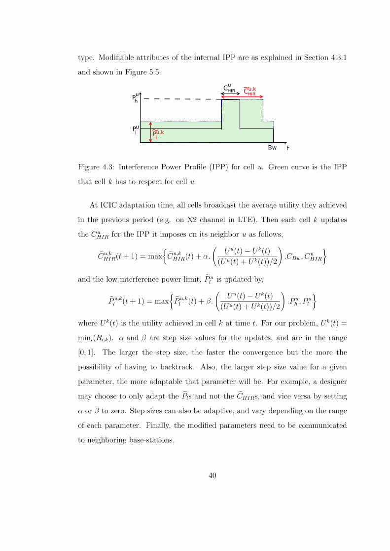
Figure 4.3: Interference Power Profile (IPP) for cell u. Green curve is the IPP

that cell k has to respect for cell u.

At ICIC adaptation time, all cells broadcast the average utility they achieved

in the previous period (e.g. on X2 channel in LTE). Then each cell k updates

the Cu

HIRfor the IPP it imposes on its neighbor u as follows,

�Cu,k

HIR(t+ 1) = max

��Cu,k

HIR(t) + α.

�Uu(t)− Uk(t)

(Uu(t) + Uk(t))/2

�

.CBw, Cu

HIR

�

and the low interference power limit, �P u

lis updated by,

�P u,k

l(t+ 1) = max

��P u,k

l(t) + β.

�Uu(t)− Uk(t)

(Uu(t) + Uk(t))/2

�

.P u

h, P u

l

�

where Uk(t) is the utility achieved in cell k at time t. For our problem, Uk(t) =

mini(Ri,k). α and β are step size values for the updates, and are in the range

[0, 1]. The larger the step size, the faster the convergence but the more the

possibility of having to backtrack. Also, the larger step size value for a given

parameter, the more adaptable that parameter will be. For example, a designer

may choose to only adapt the �Pls and not the �CHIRs, and vice versa by setting

α or β to zero. Step sizes can also be adaptive, and vary depending on the range

of each parameter. Finally, the modified parameters need to be communicated

to neighboring base-stations.

40

Table 4.1: Simulation parameters

Parameter Values

Number of cells 19, with wrap around

Users per cell for adaptive method 19-21, uniformly distributed

Site to site distance (m) 130

Bandwidth 10 MHz

Number of subbands 63

Max Power per user per band 250mW/63

Path loss model (dB) 30 log10 R, R in (m).

Fractional power control α = 1, Γ differs.

IoT ICon=10, Reuse1=13 (dB)

PF scheduling parameters a = 3.5

FFR reuse 1 band /total band η = 45/63

SFR parameters pl/ph = 1/10, γ = 6 dB

PF Scheduling at every: 1 frame (1ms)

Optimal Scheduling at every: 10 frames (10ms)

Step sizes for adaptive ICon α = β = 0.2

4.5 Simulations

We provide Monte Carlo simulations for a 19 cell hexagonal 2-D cellular network,

similar to one given in micro case for LTE [3GP06]. We use wrap around in order

41

300 400 500 600 700 800 900 1000 1100 12000

0.1

0.2

0.3

0.4

0.5

0.6

0.7

0.8

0.9

1

Rate (kbps)

CD

F

ICon with PFICon with optICon with PF, AdaptiveReuse 1SFRFFR

Figure 4.4: CDF of achieved rates in a cell using various inter-cell interference

coordination and scheduling schemes.

Table 4.2: 5 percentile rate, ICon with PF, with IoT=10 db in low interference

region.

Rate(Kbps) Pl = Ph/20 Ph/10 Ph/4 Ph/2

CHIR = 9 429.50 487.00 568.00 491.00

18 439.50 488.00 558.50 483.00

27 458.50 535.00 545.50 496.50

36 538.50 632.00 539.00 476.00

54 625.50 577.00 510.00 487.50

to avoid boundary inconsistencies. Simulation parameters are given in Table 5.1.

We simulate several common ICIC and resource allocation methods: Reuse 1,

SFR, and FFR, all with fractional power control and using proportionally fair

scheduling, with parameters given in Table 5.1. We simulate our ICIC method,

42

500 520 540 560 580 600 620 640 660 680 7000

0.05

0.1

0.15

0.2

0.25

Rate (kbps)

CD

F

ICon with PFICon with optICon with PF, AdaptiveReuse 1SFRFFR

5 percentile rate

Figure 4.5: Close-up of Fig. 4.4 demonstrating the five percentile rate achieved

in each of the methods.

ICon, with proportionally fair intra-cell scheduling, and with optimum intra-cell

scheduling given in Section 4.3.2. We perform simulations for 4 cell sizes, with

site to site distance ranging from 32.5 (m) to 260 (m).

First, to find the Pl and CHIR parameters for ICon, we find the 5 percentile

rate achieved using a range of Pl and CHIR values. An example is given in Table

4.2, which demonstrates this for site to site distance of 130 (m). In this case

Pl = Ph/10 and CHIR = 36 achieves the highest 5 percentile rate.

Figure 4.4 demonstrates the CDFs of rates achieved by users in each scheme

for site to site distance of 130 m, and Figure 5.10 is the closeup of the 5 percentile

region of the curves. Given these parameters, Reuse 1, SFR, and FFR achieve

similar 5 percentile rates, but FFR performs worse than SFR and Reuse 1 for high

rate users. ICon with both optimal and PF scheduling methods achieve higher 5

percentile rate than other methods, with 18% for ICon with PF and 20% for ICon

with optimal scheduling. Additionally, we observe that the optimal scheduling

does not achieve a much higher performance compared with PF, only about 1%

43

gain in rate. The reason for this is that the approximation of interference in the

next scheduling time as the average of the past is not accurate. Furthermore,

optimal scheduling is done once every 10 frames, whereas PF is at every frame,

which decreases the accuracy of interference prediction.

Lastly, we demonstrate the adaptation of ICon in Figure 4.6. Initially we

run the simulations with static ICon with parameters as above, until the rates

settle to fixed values. Then we start the adaptation algorithm. We plot the five

percentile rate versus the number of iterations of the adaptive method. From

the first iteration, the 5 percentile rate is instantly increased by 18 Kbps, and

eventually converges to a 5% gain over static ICon. This demonstrates both rapid

convergence and performance gain over the static case.

1 2 3 4 5 6 7635

640

645

650

655

660

665

670

Iterations

5 pe

rcen

tile

Rat

e (K

bps)

Figure 4.6: Evolution of 5 percentile rate when the ICon adaptation is allowed.

ICon with PF scheduling for site to site = 130 m, users per cell: 19-21, uniformly

distributed.

44

4.6 Conclusion

In this work we propose a new inter-cell interference management method (ICon)

for OFDMA based networks, such as LTE of 3G and WiMAX. ICon is based

on setting interference power limits on each subband for each cell, requiring the

neighboring cells to respect the imposed limits. Our simulations show that ICon

achieves up to 18% gain over reuse 1 for the 5 percentile rate in a typical cellular

network. ICon is easily and rapidly adapted to the performance obtained by each

cell, which results in balancing of the performance over the whole network.

We also propose a two phase solution to the NP-hard problem of resource

allocation in multicell OFDMA-based networks. First, ICon performs inter-cell

resource management, updating interference power limits for each cell. Second,

the intra-cell optimal scheduling assigns resources in each cell while meeting the

constraints imposed by ICon. The optimal intra-cell scheduling is found to be a

linear optimization problem for which efficient solutions exist. Static ICon with

optimal scheduling performs 20% better than reuse 1 in terms of 5 percentile

rate, and the adaptive method adds an additional 5% gain over this value.

45

CHAPTER 5

Correlation used in resource allocation for

Multi-cell networks

5.1 Introduction

In this chapter we examine a scenario where sources in a multi-cell Orthogonal

Frequency Division Multiple Access (OFDMA) network are spatially correlated,

and aim to transmit their data to the base station of their cell. An example is

shown in Figure 5.1, where the sources are scattered on a field which is divided

into three hexagonal cells. The base station in the center of each cell contains a

scheduler which is tasked with performing the resource allocation with the aim

of minimizing the maximum individual distortion achieved in the global network

after data reconstruction. Our goal is to find a strategy to allocate resources to

each source, while taking advantage of spatial correlation among the sources.

The scenario we consider in this work readily applies to Wireless Sensor Net-

works (WSNs), where sensors are scattered on a field, measuring various spatially

correlated phenomena such as temperature, humidity, audio, video, etc. [ASS02].

Since much of the surface area of interest for WSN applications is now covered

by cellular networks, it is more accessible for some WSNs to simply use this ex-

isting communication infrastructure. Therefore in this work we assume a multi

cell network with a Medium Access Control (MAC) scheme similar to LTE of 3G

46

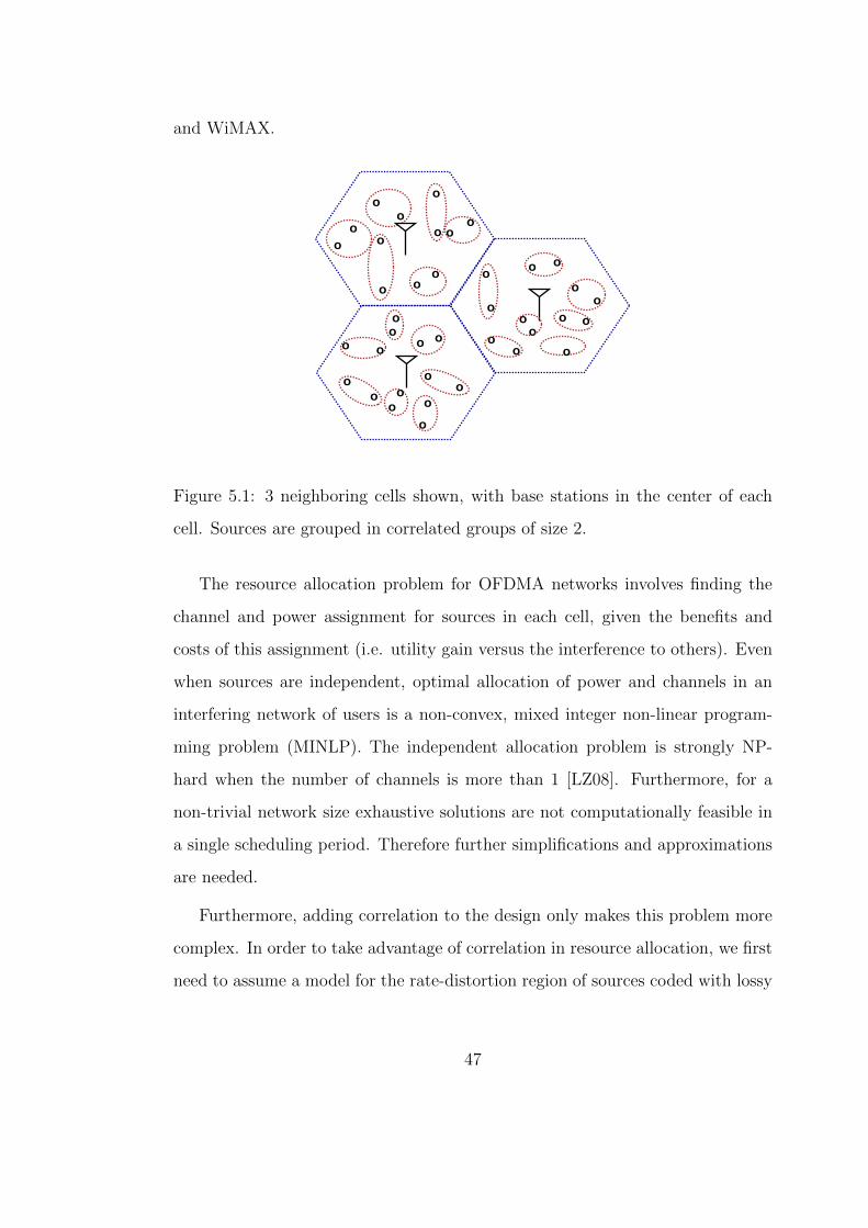
and WiMAX.

Figure 5.1: 3 neighboring cells shown, with base stations in the center of each

cell. Sources are grouped in correlated groups of size 2.

The resource allocation problem for OFDMA networks involves finding the

channel and power assignment for sources in each cell, given the benefits and

costs of this assignment (i.e. utility gain versus the interference to others). Even

when sources are independent, optimal allocation of power and channels in an

interfering network of users is a non-convex, mixed integer non-linear program-

ming problem (MINLP). The independent allocation problem is strongly NP-

hard when the number of channels is more than 1 [LZ08]. Furthermore, for a

non-trivial network size exhaustive solutions are not computationally feasible in

a single scheduling period. Therefore further simplifications and approximations

are needed.

Furthermore, adding correlation to the design only makes this problem more

complex. In order to take advantage of correlation in resource allocation, we first

need to assume a model for the rate-distortion region of sources coded with lossy

47

distributed source coding. This rate-distortion region is not known for the general

quantization resolution of the sources. However in the limit of high resolution

the region is known, as given in [ZB99]. In fact, this bound is an outer limit to

the general rate-distortion region, which tightens as the resolution increases. We

therefore assume this model for the rate-distortion region in our resource allo-

cation scheme. However, given the R-D region, now the distortion must also be

allocated among the correlated sources. Additionally, the correlation character-

istics of sources and their contribution to the performance of other sources in the

network should be considered in the resource allocation scheme. Lastly, another

design question arises from this and should be addressed, which is whether all

the correlated sources should be jointly decoded or the sources should be split

into smaller groups, and what are the costs and benefits of different group sizes.

In this chapter we present a three step approach for the problem of resource

allocation for spatially correlated sources. Namely, the three steps are called

Inter-cell resource management, Source Grouping, and Intra-cell Scheduling.

First, we find transmit power limits in each cell in the inter cell interference

management step. For this, we use the Adaptive ICon interference coordina-

tion method of the prior chapter. ICon manages the inter-cell interference by

concentrating the interference experienced by a cell base station in a designated

frequency sub-band. This results in setting transmit power limits on each sub-

band for the users of neighboring cells, and separates the global problem into

smaller problems solvable in each cell, while adaptively managing the inter-cell

interference. Adaptation is performed in order to balance the performance across

the network, and requires that at each adaptation time the decoder transmits the

utility achieved in the cell, as well as its surrounding cells.

Secondly, in the Source Grouping (SG) step we split the set of sources in

48

each cell to smaller groups to be jointly decoded. This is done in order to take

most advantage of spatial correlation without high increase in complexity in the

decoder and scheduler. We compare the utility gain of larger group sizes and

conclude that having two sources per group achieves much of the achievable cor-

relation gain. We propose a location based, adaptive SG method called Distance

Outer-Priority (distance OP). This method finds the best grouping for the cell,

while accounting for the interference to neighboring cells.

Lastly, we use the parameters found in previous steps in order to find the

channel and distortion allocation in the Intra-cell scheduling step, using two novel

scheduling methods. One scheme called Distortion Proportionally Fair (D-PF)

is based on the popular Proportionally Fair method [WOG05], modified in order

to take the effects of correlation into account. The second scheduling method is

a linear programming problem (OPT) which simultaneously finds channel and

distortion allocation for each source. OPT performs better than D-PF at the

price of higher complexity.

In the simulations we demonstrate that our proposed scheme presents a con-

structive, simple solution to the computationally infeasible optimum resource al-

location problem, superior to the existing uncorrelated resource allocation meth-

ods.

This Chapter is organized as follows. In Section 5.2 we discuss the related

work. We formulate the problem in Section 5.3, and propose our three phased

solution in Section 5.4. Then each step of the proposed solution is discussed in

Sections 5.4.1, 5.4.2, and 5.4.3. We present results of our simulations in Section

5.5.

49

5.2 Related Work

Resource allocation in this work refers to finding joint power and channel allo-

cation to sources subject to the limitations in the resources. For this problem in

cellular networks, common approaches are based on decoupling the inter-cell and

intra-cell resource management problems. For inter-cell resource management,

Fractional Frequency Reuse (FFR) and Soft Frequency Reuse (SFR) [Hal83]

[Hua05] have been proposed by the cellular industry. In these methods, a power

profile is assigned to every cell, which sets transmit power limits on each fre-

quency sub-band for OFDMA. The neighboring cells are assigned complimentary

power profiles in order to shape the inter-cell interference. These power profiles

are based on heuristics. Usually for intra-cell scheduling, the scheduler in each

cell performs channel allocation independently, using a method such as Propor-

tionally Fair scheduling [WOG05]. Although these methods are a promising step

towards simultaneous power and channel allocation, their performance is not gen-

erally better than the frequency Reuse 1 scheme [EBF08], which simply allows

the use of every frequency band at the same transmit power limit in every cell.

In order to improve on these solutions, we proposed Adaptive ICon in [BPF11].

Adaptive ICon is an adaptive inter-cell interference management method based

on concentrating the interference to a cell on a particular sub-band. This is

achieved by requiring the neighboring cells to respect an interference power profile

set by the cell. The method achieves significant improvement over FFR and SFR

schemes. Another interesting inter-cell interference management method called

inverted reuse was proposed in [GKW10], which is also based on concentrating

the interference experienced by a cell on a specific frequency band, by setting

transmit power limits for its neighboring cells.

On the other hand, the use of spatial correlation in resource allocation has

50

been studied mainly in the field of WSNs. In most WSN applications, energy sav-

ing communication is a priority [RM04]. Well-known early power saving methods

involve using 802.11-like MAC, and saving power by enabling periodic sleep-wake

cycles for wireless sensors, such as S-MAC [YHE02] and P-MAC[ZRS05]. Later

[VA06] proposed Correlation-based Collaborative Medium Access Control (CC-

MAC), which takes advantage of spatial correlation among sensors by finding

a subset of sensors to transmit their data while data from the rest is omitted.

In this work we aim to use the data from every sensor, while minimizing the

maximum distortion in the network.

A different, but related problem is studied in multi-hop WSNs, where spatial

correlation is utilized in combining routing and rate allocation with data com-

pression [PKG04] [LR09] [WPW09] [MRB11]. In [CB06] the authors propose a

method for lossy transmission of data, combining routing with rate and distortion

allocation using Wyner-Ziv (WZ) [WZ76] distributed lossy source coding. They

find that routing and rate and distortion optimization can be decoupled and op-

timized separately, when the cost function is a weighted sum of rates. Although

this is a different problem than what we are considering in this work, the ideas

developed in this area are similar to our approach to the joint power and channel

allocation problem for correlated sources.

To the best of our knowledge there is no work that proposes solutions for the

joint power and channel allocation using spatial correlation in multi-cell networks.

5.3 Problem Formulation

We consider a 2-D multi-cell network with OFDMA multiple access scheme.

Sources observe spatially correlated information, and transmit their observation

51

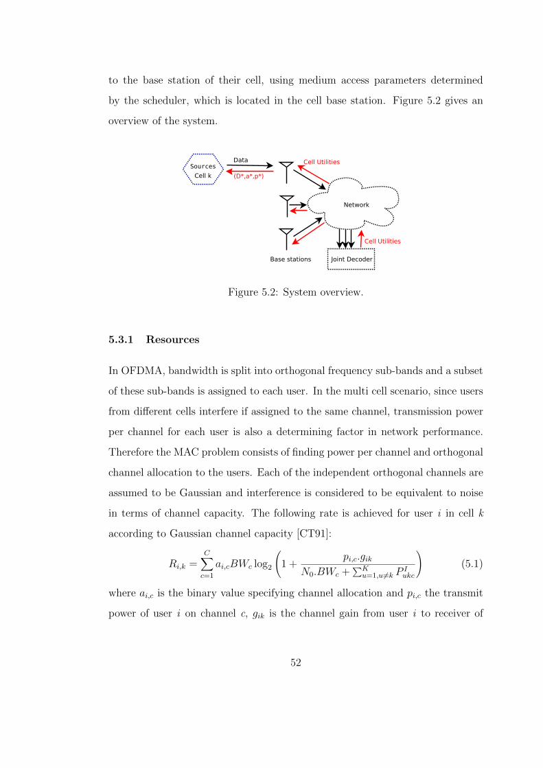
to the base station of their cell, using medium access parameters determined

by the scheduler, which is located in the cell base station. Figure 5.2 gives an

overview of the system.

Figure 5.2: System overview.

5.3.1 Resources

In OFDMA, bandwidth is split into orthogonal frequency sub-bands and a subset

of these sub-bands is assigned to each user. In the multi cell scenario, since users

from different cells interfere if assigned to the same channel, transmission power

per channel for each user is also a determining factor in network performance.

Therefore the MAC problem consists of finding power per channel and orthogonal

channel allocation to the users. Each of the independent orthogonal channels are

assumed to be Gaussian and interference is considered to be equivalent to noise

in terms of channel capacity. The following rate is achieved for user i in cell k

according to Gaussian channel capacity [CT91]:

Ri,k =C�

c=1

ai,cBWc log2

�

1 +pi,c.gik

N0.BWc +�

K

u=1,u �=kP I

ukc

�

(5.1)

where ai,c is the binary value specifying channel allocation and pi,c the transmit

power of user i on channel c, gik is the channel gain from user i to receiver of

52

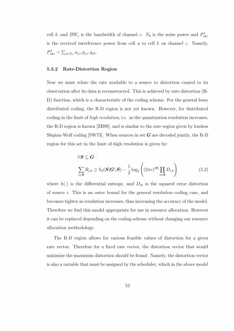
cell k, and BWc is the bandwidth of channel c. N0 is the noise power and P I

ukc

is the received interference power from cell u to cell k on channel c. Namely,

P I

ukc=

�j∈Xu

aj,c.pj,c.gjk.

5.3.2 Rate-Distortion Region

Now we must relate the rate available to a source to distortion caused to its

observation after its data is reconstructed. This is achieved by rate-distortion (R-

D) function, which is a characteristic of the coding scheme. For the general lossy

distributed coding, the R-D region is not yet known. However, for distributed

coding in the limit of high resolution, i.e. as the quantization resolution increases,

the R-D region is known [ZB99], and is similar to the rate region given by lossless

Slepian-Wolf coding [SW73]. When sources in set G are decoded jointly, the R-D

region for this set in the limit of high resolution is given by:

∀S ⊆ G :

�

i∈SRi,k ≥ h2(S|G\S)− 1

2log2

(2πe)|S| �

i∈SDi,k

(5.2)

where h(.) is the differential entropy, and Dik is the squared error distortion

of source i. This is an outer bound for the general resolution coding case, and

becomes tighter as resolution increases, thus increasing the accuracy of the model.

Therefore we find this model appropriate for use in resource allocation. However

it can be replaced depending on the coding scheme without changing our resource

allocation methodology.

The R-D region allows for various feasible values of distortion for a given

rate vector. Therefore for a fixed rate vector, the distortion vector that would

minimize the maximum distortion should be found. Namely, the distortion vector

is also a variable that must be assigned by the scheduler, which in the above model

53

would translate to quantization levels of the encoder. We now explain how G

and h(.) are found.

The set of sources that are decoded jointly, i.e. G in the above bound, can

include from only 1 source which results in independent coding, up to all the

sources in a cell, which results in taking full advantage of correlation. However,

increasing the size of joint decoding groups increases the complexity in decoding

and scheduling. Also, we later show that increasing the group size has diminishing

returns in terms of decrease in achieved distortions. Therefore we assume that

sources are decoded in smaller groups, namely we perform simulations for groups

of size one, two, and three. In this case, the choice of sources that are grouped

together in the same joint decoding group is an important factor in the resulting

distortion levels of sources. We propose an algorithm for the grouping in Section

5.4.2.

Additionally, in the R-D region given in Eq. (5.2), the source entropies must

be found. In order to find the entropies we need to model the sources as joint

random variables with some known distribution, with a distance based correlation

model. The choice of the distribution and the correlation model does not affect

our analysis, however in the simulations we use the following example. The

observations at the sources are modeled as joint Gaussian random variables, which

is commonly used in WSNs to simplify the analysis. For the correlation model

we use an exponential distance based correlation model [BDS01]. The entropy in

this example is given by,

h2(S) =1

2log2

�(2πe)|S||Σ|

�(5.3)

where |Σ| is the determinant of the covariance matrix with elements given as

54

below, when σ2 is the variance of the sources:

σ2ij= σ2.e(

−dijθ ) (5.4)

These are not assumptions of this method, but only examples that we consider

in our simulations. The only requirement for the correlation model is that corre-

lation must decrease with distance.

5.3.3 Optimization Problem

The optimization problem is to minimize the maximum distortion found in the

global network, subject to resource constraints and the R-D region. It is given

as follows.

Problem 1:

Minimizea,p,D

maxi,k

(Di,k) (5.5)

s.t.�

i∈SRi,k ≥ −1

2log2

(2πe)|S| �

i∈SDi,k

+ h2(S|G\S),

∀S ⊆ G, ∀G ⊆ Xk, ∀k�

i∈kai,c = 1 ∀k

PMIN ≤ pi,k ≤ PMAX , ∀i, k

where Ri,k is given as Eq. (5.1), and Xk is the set of all sources in cell k. The

parameters are the resource allocation vectors, a and p, as well as the source

grouping for each cell, G, such that ∪G = Xk and |G| is small. This problem

is NP-hard for C > 1 based on similar arguments given in [LZ08]. We therefore

propose in the next section to decompose this problem into three smaller steps

which can be solved efficiently.

55

5.4 Proposed Three Phase Solution

We separate the scheduling problem into three steps, as demonstrated in Figure

5.3. The three steps are performed in the scheduler, located in the base station of

every cell. The steps are called Inter-cell resource management, Source Grouping,

and Intra-cell Scheduling.

The Inter-cell resource management finds the transmit power limits for each

user on each sub band, given the location of the sources on the field, and per-

formance of the neighboring cells. We use Adaptive ICon [BPF11] for this step,

which is based on concentrating the interference to a cell on a portion of the

bandwidth. The ICon parameters are adapted in order to balance the utility

across the cellular network by increasing or decreasing interference limits of a cell

depending on its utility relative to its neighbors. The utility achieved in the cell

and its neighbors is communicated by the decoder.

Figure 5.3: Scheduler in the base stations.

In Source Grouping (SG) step, the sources are grouped together for joint

decoding (which is then used in the intra-cell scheduling step). We examine

having correlated groups of one, two, and three. We propose a distance-based SG,

which also takes the potential added interference of the sources into consideration

when finding correlated groups.

The intra-cell scheduling step involves allocating channels and distortion to

users, given the power and source grouping found in the previous steps. Given

56

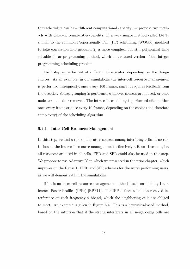
that schedulers can have different computational capacity, we propose two meth-

ods with different complexities/benefits: 1) a very simple method called D-PF,

similar to the common Proportionally Fair (PF) scheduling [WOG05] modified

to take correlation into account, 2) a more complex, but still polynomial time

solvable linear programming method, which is a relaxed version of the integer

programming scheduling problem.

Each step is performed at different time scales, depending on the design

choices. As an example, in our simulations the inter-cell resource management

is performed infrequently, once every 100 frames, since it requires feedback from

the decoder. Source grouping is performed whenever sources are moved, or once

nodes are added or removed. The intra-cell scheduling is performed often, either

once every frame or once every 10 frames, depending on the choice (and therefore

complexity) of the scheduling algorithm.

5.4.1 Inter-Cell Resource Management

In this step, we find a rule to allocate resources among interfering cells. If no rule

is chosen, the Inter-cell resource management is effectively a Reuse 1 scheme, i.e.

all resources are used in all cells. FFR and SFR could also be used in this step.

We propose to use Adaptive ICon which we presented in the prior chapter, which

improves on the Reuse 1, FFR, and SFR schemes for the worst performing users,

as we will demonstrate in the simulations.

ICon is an inter-cell resource management method based on defining Inter-

ference Power Profiles (IPPs) [BPF11]. The IPP defines a limit to received in-

terference on each frequency subband, which the neighboring cells are obliged

to meet. An example is given in Figure 5.4. This is a heuristics-based method,

based on the intuition that if the strong interferers in all neighboring cells are

57

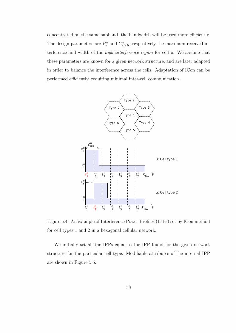
concentrated on the same subband, the bandwidth will be used more efficiently.

The design parameters are P u

hand Cu

HIR, respectively the maximum received in-

terference and width of the high interference region for cell u. We assume that

these parameters are known for a given network structure, and are later adapted

in order to balance the interference across the cells. Adaptation of ICon can be

performed efficiently, requiring minimal inter-cell communication.

Figure 5.4: An example of Interference Power Profiles (IPPs) set by ICon method

for cell types 1 and 2 in a hexagonal cellular network.

We initially set all the IPPs equal to the IPP found for the given network

structure for the particular cell type. Modifiable attributes of the internal IPP

are shown in Figure 5.5.

58

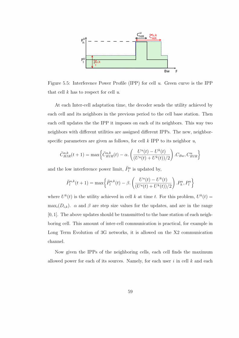
Figure 5.5: Interference Power Profile (IPP) for cell u. Green curve is the IPP

that cell k has to respect for cell u.

At each Inter-cell adaptation time, the decoder sends the utility achieved by

each cell and its neighbors in the previous period to the cell base station. Then

each cell updates the the IPP it imposes on each of its neighbors. This way two

neighbors with different utilities are assigned different IPPs. The new, neighbor-

specific parameters are given as follows, for cell k IPP to its neighbor u,

�Cu,k

HIR(t+ 1) = max

��Cu,k

HIR(t)− α.

�Uu(t)− Uk(t)

(Uu(t) + Uk(t))/2

�

.CBw, Cu

HIR

�

and the low interference power limit, �P u

lis updated by,

�P u,k

l(t+ 1) = max

��P u,k

l(t)− β.

�Uu(t)− Uk(t)

(Uu(t) + Uk(t))/2

�

.P u

h, P u

l

�

where Uk(t) is the utility achieved in cell k at time t. For this problem, Uk(t) =

maxi(Di,k). α and β are step size values for the updates, and are in the range

[0, 1]. The above updates should be transmitted to the base station of each neigh-

boring cell. This amount of inter-cell communication is practical, for example in

Long Term Evolution of 3G networks, it is allowed on the X2 communication

channel.

Now given the IPPs of the neighboring cells, each cell finds the maximum

allowed power for each of its sources. Namely, for each user i in cell k and each

59

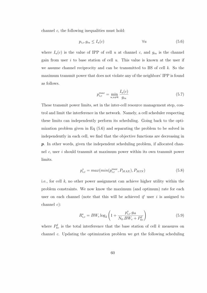
channel c, the following inequalities must hold:

pi,c.giu ≤ Iu(c) ∀u (5.6)

where Iu(c) is the value of IPP of cell u at channel c, and giu is the channel

gain from user i to base station of cell u. This value is known at the user if

we assume channel reciprocity and can be transmitted to BS of cell k. So the

maximum transmit power that does not violate any of the neighbors’ IPP is found

as follows.

pmax

i,c= min

u,u �=k

Iu(c)

giu(5.7)

These transmit power limits, set in the inter-cell resource management step, con-

trol and limit the interference in the network. Namely, a cell scheduler respecting

these limits can independently perform its scheduling. Going back to the opti-

mization problem given in Eq (5.6) and separating the problem to be solved in

independently in each cell, we find that the objective functions are decreasing in

p. In other words, given the independent scheduling problem, if allocated chan-

nel c, user i should transmit at maximum power within its own transmit power

limits.

p∗i,c

= max(min(pmax

i,c, PMAX), PMIN) (5.8)

i.e., for cell k, no other power assignment can achieve higher utility within the

problem constraints. We now know the maximum (and optimum) rate for each

user on each channel (note that this will be achieved if user i is assigned to

channel c):

R∗i,c

= BWc log2

�

1 +p∗i,c.gik

N0.BWc + P I

kc

�

(5.9)

where P I

kcis the total interference that the base station of cell k measures on

channel c. Updating the optimization problem we get the following scheduling

60

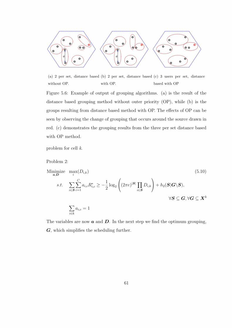
(a) 2 per set, distance based

without OP.

(b) 2 per set, distance based

with OP.

(c) 3 users per set, distance

based with OP

Figure 5.6: Example of output of grouping algorithms. (a) is the result of the

distance based grouping method without outer priority (OP), while (b) is the

groups resulting from distance based method with OP. The effects of OP can be

seen by observing the change of grouping that occurs around the source drawn in

red. (c) demonstrates the grouping results from the three per set distance based

with OP method.

problem for cell k.

Problem 2:

Minimizea,D

maxi

(Di,k) (5.10)

s.t.�

i∈S

C�

c=1

ai,cR∗i,c

≥ −1

2log2

(2πe)|S| �

i∈SDi,k

+ h2(S|G\S),

∀S ⊆ G, ∀G ⊆ Xk

�

i∈kai,c = 1

The variables are now a and D. In the next step we find the optimum grouping,

G, which simplifies the scheduling further.

61

5.4.2 Grouping of Correlated Sources

In order to take advantage of correlation in this problem setting, sources need

to be decoded jointly. The number of sources that are jointly decoded can theo-

retically be as many as all the sources in a cell, and as little as two sources per

decoding group, with correlation benefits increasing with more sources decoded

jointly. However, as we will show in this section, increasing the group size beyond

two or three sources per group does not offer significant benefits in terms of dis-

tortion. Additionally, complexities of both decoding and cross layer scheduling

increase with the number of sources involved in joint decoding. Therefore in this

work we assume that only a small number of sources can be decoded jointly, i.e.

two or three. Initially, we assume the size of groups is set and fixed. Given this

fixed group size, in this step the scheduler has to find which sources are grouped

together and jointly decoded.

Grouping affects the performance in two ways, directly and indirectly. The

direct effect refers to the performance a cell achieves as a result of jointly decoding

the given groups of sources together. Specifically, the correlation levels of sources

that are grouped together and the channel rate each source achieves affect the

utility of the cell after the particular groups of sources are decoded jointly. On

the other hand, the indirect effect refers to the impact of the particular group-

ing method on the cross-layer resource allocation strategy, and therefore on the

interference levels in the network, which results in change in the utility achieved

in each cell.

The indirect effect of grouping is difficult to predict, especially since it involves

knowledge of the load in nearby cells. However, the direct effect of a particular

grouping of sources can be found using the rate-distortion region given in Eq

(5.2), if data rates of the sources are assumed fixed. In order to simplify the

62

analysis, we demonstrate this effect for a group of two correlated sources. The

joint rate-distortion region is given by the following three inequalities:

45 degree line !1+1/2.log2(2"e)

-R1+h(x1)

-R1+h(x1|x2)

-R2+h(x2|x1) -R2+h(x2) !2+1/2.log2(2"e)

Figure 5.7: Trade-off of distortions for two correlated users.

R1 ≥ h2(X1|X2)−1

2log2 (2πeD1)

R2 ≥ h2(X2|X1)−1

2log2 (2πeD2)

R1 +R2 ≥ h2(X1, X2)−1

2log2

�(2πe)2D1D2

�

We define ∆i = 1/2 log2 Di to simplify the notation. For fixed rates, ∆i values

are bounded by:

∆1 ≥ −R1 + h2(X1|X2)−1

2log2(2πe) (5.11)

∆2 ≥ −R2 + h2(X2|X1)−1

2log2(2πe)

∆1 +∆2 ≥ −R1 −R2 + h2(X1, X2)− log2(2πe)

This region is demonstrated in Figure 5.7. When the aim is to minimize the

maximum distortion, the following conditions determine the outcome of assigning

63

distortion to users:

if −Ri + h2(Xi|Xj) ≥ −Rj + h2(Xj) (5.12)

then ∆i = −Ri + h2(Xi|Xj)−1

2log2(2πe)

and ∆j = −Ri + h2(Xj)−1

2log2(2πe)

for i=1, j = 2, and vice versa. If neither condition is met, then the distortions

will be equal:

∆1 =1

2[−R1 −R2 + h2(X1, X2)− log2(2πe)]

∆2 = ∆1. (5.13)

Conditions (5.12) and (5.13) can be directly observed in Figure 5.7, by intersect-

ing the R-D region with the line ∆1 = ∆2, which is the line that minimizes the

maximum ∆i. Note that in each of the above conditions one of the three inequal-

ities given in Eq. (5.11) is met with equality. This applies to higher number of

users per set as well [ZB99].

However, these conditions cannot be used to exactly predict the achieved

distortion in a cell as a result of a particular source grouping. The reason is

that the assumption of fixed data rates for sources is not realistic in a cross-layer

resource allocation strategy, since the rate assigned to each source is affected by

the source grouping method. Additionally, the above conditions only consider

the direct effect of grouping on distortion, and ignore the effects of the particular

grouping on the resource allocation, and therefore the interference in the network,

and the resulting change in distortion of the sources in each cell. Therefore, an

exhaustive solution cannot find the optimum source grouping using the above

conditions, and is not computationally feasible in a reasonable timeline. However,

from the above we learn a few valuable lessons that we use in constructing our

grouping methods.

64

One is that the direct benefit of joint decoding is larger when sources are

grouped such that the intra-group correlation is maximized. Additionally, the

channel quality of sources in a group affect the final correlation gain of a source.

As an example, if a source is jointly decoded with sources that have very low

data rates, the correlation benefit it achieves is small, even if correlation level is

high among the group.

Additionally, we must take the indirect effects of grouping into account. For

this, we compare two source groupings that achieve the same direct correlated

utility benefits, one which results in less need for transmission by a source located

in the outer region of a cell. The grouping that results in less need for outer-user

transmission results in lower interference levels in the network, and therefore less

need for neighboring cells to increase their transmission power, thus achieving

lower distortion in the network. Figure 5.6 demonstrates an example with two

source groupings, one which takes the indirect effect into account and one that

does not.

For source grouping, we propose two constructive, simple solutions to an NP-

hard problem that cannot be solved exhaustively in real time. Each method is

appropriate for a different problem setting. The first is distortion based group-

ing with outer priority (Distortion OP), which can be used for static networks,

where sources are not added or removed, and channel conditions can be assumed

constant.

Distortion based grouping with OP : Initially perform independent de-

coding until system performance is stable. Once performance stabilizes, pick a

random source from N outer-most sources in the cell (we choose N=3 in sim-

ulations) and compute its projected performance if it is paired with any of the

other sources in the cell, using conditions in (5.12) and (5.13). Choose the pairing

65

which results in the lowest projected distortion for the chosen source and remove

the pair from the set. Repeat until no nodes remain. Find the projected distor-

tion in the cell if this grouping is used. Repeat the method T times and choose

the source grouping that achieves the lowest projected distortion in the cell (T is

chosen to be 10 in our simulations).

The second method is distance based grouping with outer priority (Distance

OP) which is an adaptive method appropriate for non-static networks. This

method does not use the R-D region to find the grouping, and simply uses the

fact that the correlation decreases with distance between cells.

Distance based grouping with OP : Pick a random source from three

outer-most sources in the cell and pair it with its closest neighbor and remove

the pair from the set. Repeat until no nodes remain. Calculate sum of inter-group

distances in the cell if this grouping is used. Repeat the method 10 times and

choose the source grouping that achieves the lowest sum of inter-group distances.

When grouping is performed on more than two sources, the tradable log dis-

tortion is:

δ∆ =

h2(S)−�

Xi∈Sh2(Xi)

|S| = N. (5.14)

If all users have equal independent distortion levels, each users’ distortion is

decreased by δ∆N

as a result of joint decoding, when the aim is to minimize the

maximum distortion. We plot this value for various set sizes, with entropy given

by Eq (5.3), covariance matrix given by Eq (5.4), and with distances assumed

equal (although even for a 3 dimensional space this is only possible for up to five

nodes). Figure 5.8 demonstrates the diminishing returns of set size. Additionally

having large sets increases the Slepian-Wolf decoder complexity, as well as intra-

cell scheduling complexity. Therefore we generally consider grouping of only a

66

small number of sources and we compare performance of two and three nodes per

set in the simulation section.

1 2 3 4 5 6 7 8 9 10−4.5

−4

−3.5

−3

−2.5

−2

−1.5

−1

−0.5

0

Cha

nge

in D

isto

rtion

(dB)

Size of correlated sets

Figure 5.8: Diminishing returns of increasing correlated set size on distortion.

When this step is performed, the scheduler of cell k has an updated source

grouping (i.e. G∗ in Eq. (5.10)). Given this value and p∗ found in the previous

step, the intra-cell scheduling unit now can find the channel allocation.

5.4.3 Intra-Cell Scheduling

In the previous phases of the three step strategy we found p∗ and G∗, power and

source grouping. In this last step we find a∗ and D∗, namely the channel and

distortion allocation to each user for the frames in the given scheduling period.

We propose two solutions for this phase, with different complexities and per-

formances. For schedulers with low computational capacity, we propose Distor-

tion Proportionally Fair (D-PF). This solution is similar to the proportionally

fair (PF) scheduling method [WOG05], modified to use distortion as utility in-

stead of rate, and to take correlation effects into account. D-PF scheduling can

be performed at every frame, similar to how PF is commonly used. As we will

67

later show in the simulations, D-PF achieves better performance that PF, as a

result of accounting for correlation in resource allocation.

The second solution we propose is called OPT, and is for schedulers with

higher computational capacity, specifically ones that are capable of solving a

linear programming scheduling problem at every scheduling period. OPT is a

relaxed optimal assignment of channels and distortions, i.e. the relaxed version

of Problem 2 given in (5.10). This problem is polynomial time solvable. Addi-

tionally, in the simulations we show that performing OPT scheduling once every

ten frames still achieves better performance than the D-PF.

5.4.3.1 D-PF scheduling

With the common proportionally fair scheduling, at each frame the user which

maximizes the following ratio is assigned channel c [WOG05]:

i = argmaxj

�R∗

j,c

Rα

j

�

⇒ a∗i,c

= 1, a∗j,c

= 0, ∀j �= i.

R∗i,c

is the possible rate achieved for user i on channel c is given by Eq (5.9)

and α is a parameter used to vary the trade-off between fairness and sum-rate

maximization. Rj is the exponentially averaged rate of user j at time t-1, given

by the following at time t by,

Rj(t) = (1

NT

).C�

c=1

Rj,c(t) + (1− 1

NT

).Rj(t− 1).

This scheduling method is simple, yet performs almost the same as relaxed opti-

mal channel allocation for independent sources, as we demonstrated in [BPF11].

However, for correlated sources it is not sufficient to maximize the above ratio,

since the effects of joint decoding are ignored.

For this, we first define D∗i,c

as the possible distortion achieved by user i if

scheduled on channel c. In order to find this value, we must use conditions (5.12)

68

and (5.13) in Section 5.4.2, given the source grouping found in the previous step of

the algorithm. These conditions require the knowledge of the values of possible

data rate that source i achieves if assigned channel c in the next scheduling

period, as well as the data rates of its correlated group members, which are

therefore not assigned channel c. We assume that for every c, Ri = R∗i,c, and

Rj = 0 for j ∈ G∗(i) and j �= i. Given these possible data rates, then we can use

the conditions (5.12) and (5.13) to find Di,c and Dj.

We now propose D-PF, which uses the following condition for scheduling user

l to channel c:

l = argmini

Di,c

Dα

i

.�

j∈G∗(i)

Dj

Dα

j

⇒ a∗l,c

= 1, a∗i,c

= 0, ∀i �= l.

where Dj is the exponentially averaged distortion of user j at time t-1, given by

the following at time t :

Dj(t) = (1

NT

).D∗j(t) + (1− 1

NT

).Dj(t− 1) (5.15)

And D∗j(t) is found at each scheduling period after the channel assignment matrix

(a∗) is found, using the conditions (5.12) and (5.13) with rates equal to Ri =�

C

c=1 a∗i,c.R∗

i,c. The output of this method is then the matrix a∗ and vector D∗,

which are transmitted to the sources at every scheduling period. The above

conditions can be readily generalized to more than two correlated sources per

decoding group, with the conditions (5.12) and (5.13) replaced by the inequality

set 5.2, solved for decreasing the maximum distortion.

5.4.3.2 OPT scheduling

Each cell finds the scheduling matrix, a∗, and distortion vector,D∗ by minimizing

the maximum distortion in the cell. For this, we use Problem 2 given in (5.10),

69

and relax it to become a linear programming problem. Namely, the values of a

are relaxed to be real valued, allowing for time-sharing of each channel between

users. Specifically, we perform OPT scheduling once every 10 frames and the real

valued vector, a, is rounded to achieve that resolution. The problem becomes

the following:

Problem 3:

Minimizea,∆

maxi

(∆i +∆i)

�

i∈S

C�

c=1

ai,cR∗i,c

≥ h2(S|G∗\S) +�

i∈S∆i −

|S|2

log2 (2πe) ,

∀S ⊆ G∗, ∀G∗ ⊆ Xk

�

i∈kai,c = 10, 0 ≤ ai,c ≤ 10 ∀i, ∀c.

∆i is log10 Di, given by Eq (5.15), and R∗i,c

is given by Eq (5.9). This is a linear

programming problem in a and ∆, solvable in polynomial time using a method

such as the Simplex algorithm [BV04]. After this problem is solved, matrix a is

found by rounding a such that each c is assigned to a single source in every frames

in the following scheduling period. Then D is found using the conditions (5.12)

and (5.13) with rates equal to Ri =�

C

c=1 a∗i,c.R∗

i,c. As with the case of D-PF, the

matrix a and vector D are then transmitted to users, determining the resource

and distortion allocation in the following scheduling period. We compare these

two scheduling methods in the simulations section.

5.5 Simulations

We simulate a 19 cell hexagonal 2-D cellular network, comparable to one given

for the micro test case for LTE [3GP06], with wrap around in order to avoid

boundary inconsistencies. In each instance of the problem, 18 sources are placed

70

with uniform distribution in every cell. Simulation parameters are given in Table

5.1. We use CDF of distortion values and rates achieved by sources in order to

demonstrate the performance of different algorithms. Since the aim in this work

is to minimize the maximum distortion achieved in the network, the parameter

we look for is the performance of 5 percentile worst performing users (5 percentile

rate and 95 percentile distortion). We begin by comparing performance of various

methods for each step of the three step algorithm, in order to justify the choices we

have made in the proposed scheme. Later we will compare the overall performance

gain of utilizing correlation in resource allocation using our proposed scheme,

versus independent allocation of resources. Finally, we demonstrate convergence

of the proposed algorithm.

In order to compare inter-cell resource management methods, we simulate

FFR, SFR, Reuse 1, static ICon, and Adaptive ICon schemes. In this step we do

not use correlation, since we would like to isolate the effects of inter-cell resource

management methods. We compare the CDFs of distortions and rates achieved

by sources, as shown in Figures 5.9(a) and 5.9(b), with 5 percentile distortion

details shown in Figure 5.10. We observe that using our static ICon inter-cell

interference management method compared with reuse 1, FFR, and SFR, the 95

percentile distortion is decreased by 0.75 dB. FFR, SFR and Reuse 1 perform

similarly, with Reuse 1 having a slight advantage, as we expected. With little

base station communication between neighboring cells, using Adaptive ICon, this

gain is increased to 1 dB.

We now add correlation to resource allocation in order to compare source

grouping methods in Figure 5.12. We use D-PF for intra-cell allocation, and use

that for all methods in this step. We first the two grouping methods we proposed

in Figure 5.12(a), namely distance OP and distortion OP. We also show the effects

71

1 2 3 4 5 6 7 80

0.1

0.2

0.3

0.4

0.5

0.6

0.7

0.8

0.9

1

D (dB)

CD

F of

Dis

torti

on

Adaptive IConIConReuse 1FFRSFR

(a) Comparison of distortion of various inter-

cell resource management methods.

0 0.2 0.4 0.6 0.8 1 1.2 1.4 1.6 1.8 20

0.1

0.2

0.3

0.4

0.5

0.6

0.7

0.8

0.9

1

Rate (bps)

CD

F of

Rat

e

Adaptive IConIConReuse 1FFRSFR

(b) Comparison of rate of various inter-cell re-

source management methods.

Figure 5.9: Inter-cell scheduling methods.

of using outer priority in this plot. We find that distortion OP performs slightly

better than distance OP, however distortion OP cannot be used adaptively, and

thus is not appropriate for some applications. We also compare the effects of

group size in Figure 5.12(b). Increasing set size from one user per group (i.e.

independent decoding) to two decreases the 95 percentile distortion by 2 dB.

However, there is almost no difference in this value when we increase the group

size from two to three sources, which is expected as explained in Section 5.4.2.

We compare the intra-cell scheduling methods, namely, PF, D-PF, and OPT,

with the inter-cell method given by static ICon and source grouping of 2 per set

distance OP for all comparisons. Results are demonstrated in Figure 5.11. We

observe that using correlation in resource allocation, even with a simple method,

i.e. D-PF compared with PF, decreases the 95 percentile distortion by 0.75 dB.

Using OPT scheduling decreases this performance metric by 1 dB more over the

D-PF, adding up to 1.75 dB over PF scheduling. This is a large gain, which

is feasible if the scheduler has the computational capacity to perform OPT, as

discussed in Section 5.4.3.

72

5.2 5.4 5.6 5.8 6 6.2 6.4 6.6 6.8

0.8

0.85

0.9

0.95

1

D (dB)

CD

F of

Dis

torti

on

Adaptive IConIConReuse 1FFRSFR

5 percentile

Figure 5.10: Closeup of distortion CDF of inter-cell resource management meth-

ods..

In Figure 5.13(a) we demonstrate the overall performance of the three phased

strategy, with adaptive ICon, two users per set distance based with OP source

grouping, and optimal intra-cell scheduling, with a baseline method, namely

Reuse 1 without spatial correlation and PF scheduling, common in cellular net-

works. Overall, we demonstrate that this method achieves a large improvement

of almost a 4 dB (60%) decrease in distortion for 5 percentile users.

Finally we show the convergence behavior of the three step algorithm in Figure

5.13(b). Each iteration shown in the Figure is 1 iteration of adaptive ICon (inter-

cell resource management step), which in our simulations is equal to 100 intra-cell

scheduling periods. This demonstrates that ICon adaptation converges almost

fully after one inter-cell resource management period.

5.6 Conclusion

In this work we consider the problem of resource allocation to spatially correlated

sources in OFDMA multi-cell networks, which is an NP-hard problem for which

73

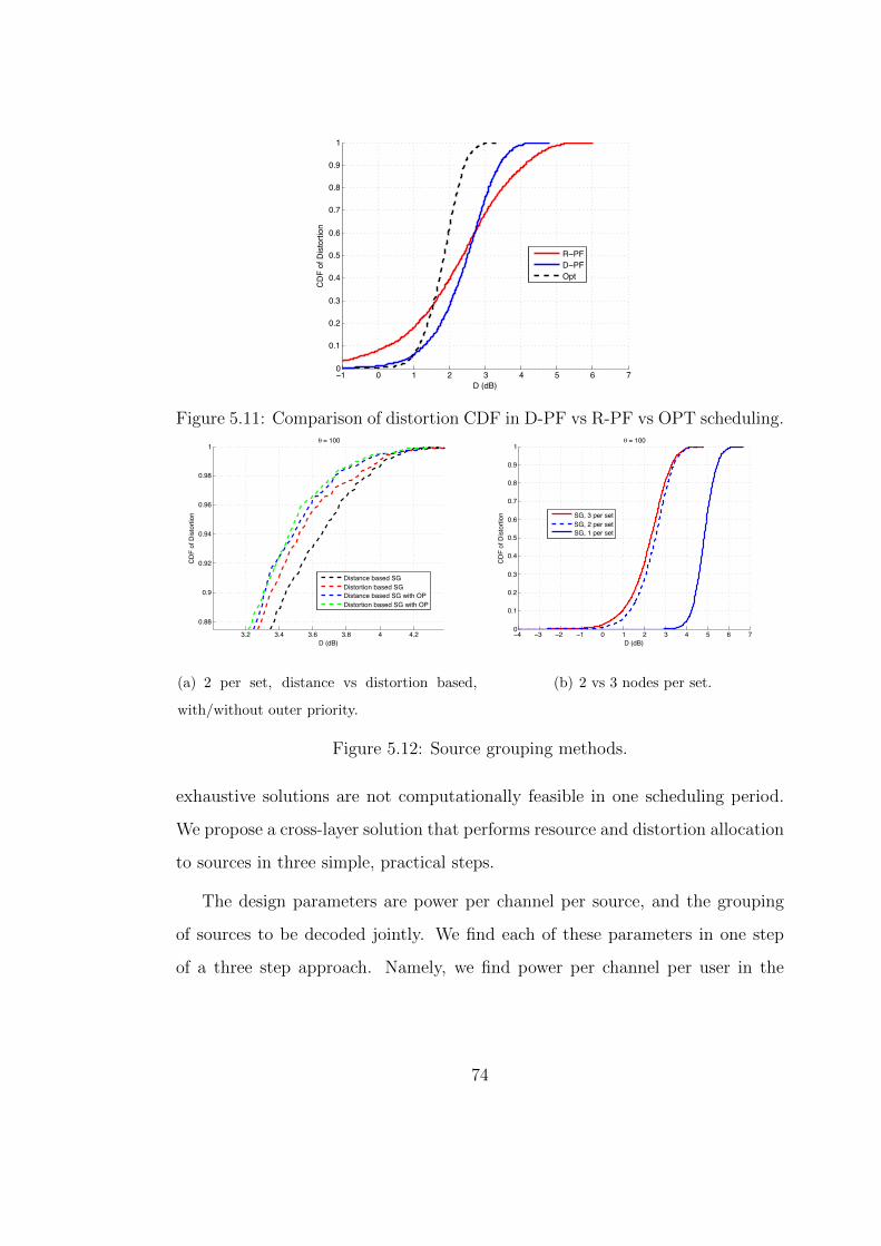
−1 0 1 2 3 4 5 6 70

0.1

0.2

0.3

0.4

0.5

0.6

0.7

0.8

0.9

1

D (dB)

CD

F of

Dis

torti

on

R−PFD−PFOpt

Figure 5.11: Comparison of distortion CDF in D-PF vs R-PF vs OPT scheduling.

3.2 3.4 3.6 3.8 4 4.2

0.88

0.9

0.92

0.94

0.96

0.98

1

D (dB)

CD

F of

Dis

torti

on

θ = 100

Distance based SGDistortion based SGDistance based SG with OPDistortion based SG with OP

(a) 2 per set, distance vs distortion based,

with/without outer priority.

−4 −3 −2 −1 0 1 2 3 4 5 6 70

0.1

0.2

0.3

0.4

0.5

0.6

0.7

0.8

0.9

1

D (dB)

CD

F of

Dis

torti

on

θ = 100

SG, 3 per setSG, 2 per setSG, 1 per set

(b) 2 vs 3 nodes per set.

Figure 5.12: Source grouping methods.

exhaustive solutions are not computationally feasible in one scheduling period.

We propose a cross-layer solution that performs resource and distortion allocation

to sources in three simple, practical steps.

The design parameters are power per channel per source, and the grouping

of sources to be decoded jointly. We find each of these parameters in one step

of a three step approach. Namely, we find power per channel per user in the

74

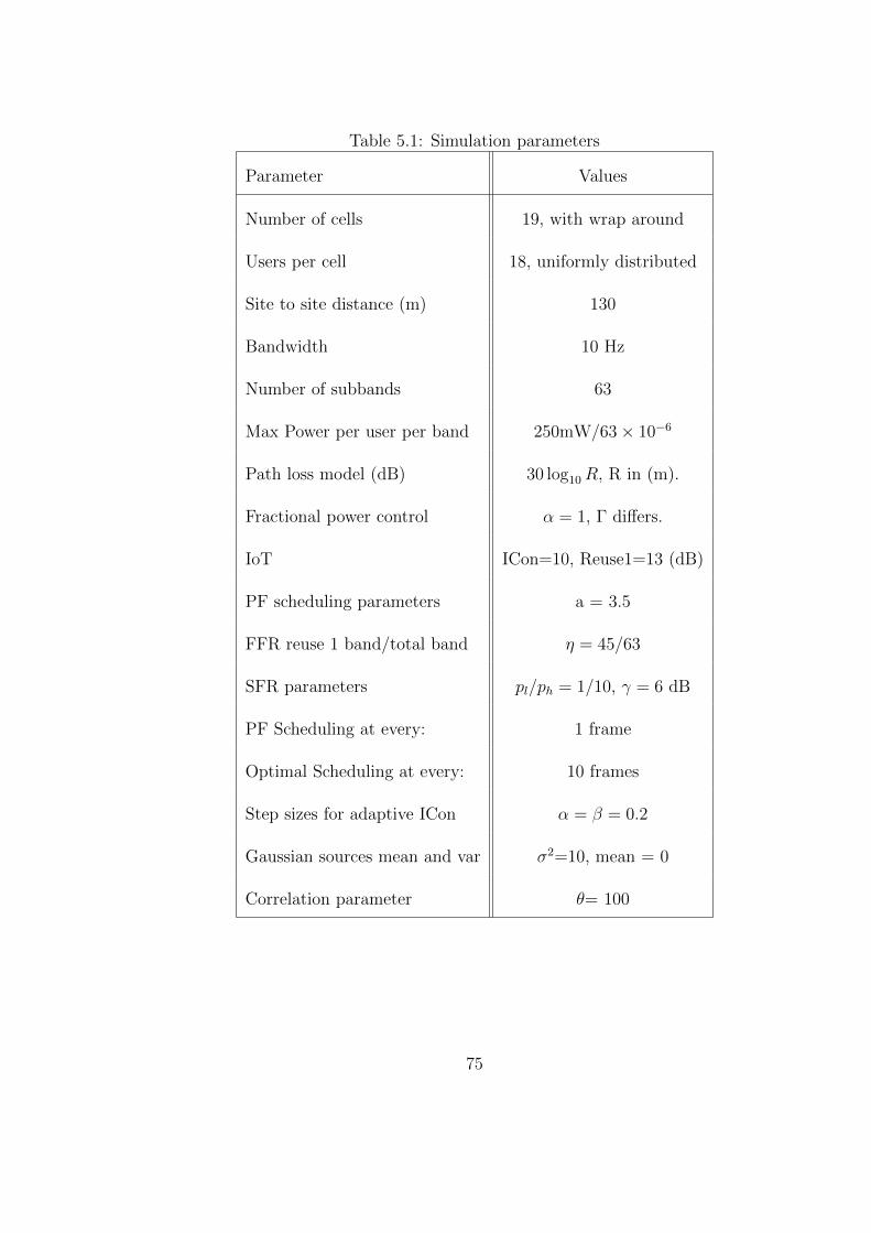
Table 5.1: Simulation parameters

Parameter Values

Number of cells 19, with wrap around

Users per cell 18, uniformly distributed

Site to site distance (m) 130

Bandwidth 10 Hz

Number of subbands 63

Max Power per user per band 250mW/63× 10−6

Path loss model (dB) 30 log10 R, R in (m).

Fractional power control α = 1, Γ differs.

IoT ICon=10, Reuse1=13 (dB)

PF scheduling parameters a = 3.5

FFR reuse 1 band/total band η = 45/63

SFR parameters pl/ph = 1/10, γ = 6 dB

PF Scheduling at every: 1 frame

Optimal Scheduling at every: 10 frames

Step sizes for adaptive ICon α = β = 0.2

Gaussian sources mean and var σ2=10, mean = 0

Correlation parameter θ= 100

75

−1 0 1 2 3 4 5 6 70

0.1

0.2

0.3

0.4

0.5

0.6

0.7

0.8

0.9

1

D (dB)

CD

F of

Dis

torti

on

Adaptive ICon+2 per set+OptimalReuse 1+1 per set+ R−PF

(a) Comparison of proposed method v baseline.

1 2 3 4 5 6 7 8 9 102

2.5

3

3.5

4

4.5

5

5.5

6

6.5

7

Iterations

5 pe

rcen

tile

Dis

torti

on (d

B)

Adap ICon+Corr+OPTICon+Corr+OPTICon+Uncorr+PFICon+Coor+D−PFAdap ICon+Coor+D−PFReuse 1+Uncorr+PF

ICon adaptation starts

Correlated decoding starts

(b) Convergence of adaptive method.

Figure 5.13: Intra-cell scheduling methods.

inter-cell resource management step, grouping of sources for joint decoding in

the source grouping step, and the channel and distortion allocation to each user

in the intra-cell scheduling step.

We justify our design choices in the simulations by comparing various methods

for each step of the algorithm. Overall, the performance gain over base-line,

non-correlated method is a 4 dB (i.e. 60%) decrease in distortion of the worst

performing sources.

76

CHAPTER 6

Concluding Remarks

In this work we proposed workable algorithms for adaptive resource allocation

for correlated sources in specific systems, namely, for single cell multi-view video

systems, and multi-cell networks with general correlated sources. Additionally,

we proposed an inter-cell interference management for multi-cell systems.

First, we proposed an adaptive resource allocation scheme for multi-view

video sources. This case was considered in order to demonstrate the benefits

of correlation-aware resource allocation in an end to end system design. We used

a simple joint decoding scheme based on the common H.264 standard, and mod-

eled the boundary of the R-D region as a piecewise linear function. We showed

that even with a simplistic coding scheme which achieves little gain over inde-

pendent coding, the correlation-aware resource allocation achieves much gain over

independent resource allocation. A more sophisticated joint decoding scheme and

R-D region associated with it could be used in our proposed method, which would

lead to higher gains.

We then considered resource allocation in multi-cell OFDMA networks. The

challenge here is to manage the inter-cell interference. We proposed a heuristics

based method called ICon, which sets interference power limits on each subband

for each cell, concentrating the interference to a cell on a designated band. This

allows for more efficient use of the bandwidth compared to the common inter-cell

interference methods such as FFR and SFR. In order to balance the performance

77

across the cells, the high interference band for each cell is rapidly and efficiently

adapted. This method can easily be utilized in Long Term Evolution of 3G

networks.

Finally we studied the problem of resource allocation to spatially correlated

sources in OFDMAmulti-cell networks. This is an NP-hard problem for which ex-

haustive solutions are not computationally feasible in a single scheduling period.

For this problem we proposed a location based, three step cross-layer resource al-

location algorithm, which takes both inter-cell interference and correlation char-

acteristics of sources into consideration. Our method achieves significant gain

over independent resource allocation with little increase in complexity.

By studying different instances of the resource allocation problem, in this

thesis we demonstrated that for networks of correlated sources, the correlation-

aware resource allocation (RA) problem achieves much gain over independent

methods. In each case we proposed practical RA schemes. An interesting future

research direction of this work is to characterize the effects of uncertainty in the

correlation model and the high-resolution R-D bound on the performance of the

correlation-aware RA.

78

References

[20006] 802.16e 2005. “Part 16: air interface for fixed and mobile broadbandwireless access systems.” Feb. 2006.

[3GP06] 3GPP. “Physical Layer Aspects for Evolved UTRA.” TR 25.814,V1.2.2 2006.

[ASS02] I. F. Akyildiz, W. Su, Y. Sankarasubramaniam, and E. Cayirci. “Wire-less Sensor Networks: a Survey.” Comput. Netw., 38:393–422, March2002.

[BDS01] J. O. Berger, V. De Oliveira, and B. Sans. “Objective Bayesian Anal-ysis of Spatially Correlated Data.” Journal of the American Statistical

Association, 96(456):1361–1374, 2001.

[BPF11] D. Bandari, G. Pottie, and P. Frossard. “ICon: Interference Concen-tration for Uplink in MultiCell OFDMA Networks.” In Proceedings

of Wireless and Mobile Computing, Networking and Communications

(WiMob), Shanghai, China, 2011.

[BV04] S. Boyd and L. Vandenberghe. Convex Optimization. Cambridge UnivPress, Cambridge, U.K., 2004.

[CB06] R. Cristescu and B. Beferull-Lozano. “Lossy Network Correlated DataGathering with High-Resolution Coding.” IEEE Transactions on In-

formation Theory, 52(6):2817 – 2824, June 2006.

[CF05] J. Chakareski and P. Frossard. “Distributed Packet Scheduling ofMultiple Video Streams over Shared Communication Resources.” InMultimedia Signal Processing, 2005 IEEE 7th Workshop on, pp. 1 –4,oct. 2005.

[Cha06] Jacob Chakareski. “Distributed media cooperation for enhanced videocommunication.” Journal of Zhejiang University - Science A, 7:773 –783, 2006.

[CT91] T. M. Cover and J. A. Thomas. Elements of Information Theory.Wiley-Interscience, New York, NY, USA, 1991.

[DN05] M. van Der Schaar and Sai Shankar N. “Cross-layer wireless multime-dia transmission: challenges, principles, and new paradigms.” Wire-

less Communications, IEEE, 12(4):50 – 58, aug. 2005.

79

[EBF08] S.E. Elayoubi, O. Ben Haddada, and B. Fourestie. “Performance Eval-uation of Frequency Planning Schemes in OFDMA-based Networks.”IEEE Transactions on Wireless Communications, 7(5):1623 –1633,May 2008.

[FSC10] Minghai Feng, Xiaoming She, and Lan Chen. “Coordinated Schedul-ing based on Overload Indicator for LTE / LTE-A Uplink.” In Vehic-

ular Technology Conference, 2010.

[GB11] Michael Grant and Stephen Boyd. “CVX: Matlab Software for Disci-plined Convex Programming.” http://cvxr.com/cvx/, April 2011.

[Gen04] 3rd Generation Partership Project 2 (3GPP2). “CDMA2000 high ratepacket data air interface specification revision a. Technical ReportC.S20024-A.” March 2004.

[GKW10] C. G. Gerlach, I. Karla, A. Weber, L. Ewe, H. Bakker, E. Kuehn,and A. Rao. “ICIC in DL and UL with network distributed and self-organized resource assignment algorithms in LTE.” Bell Labs Techni-

cal Journal, 15(3):43–62, 2010.

[Gol05] Andrea Goldsmith. Wireless Communications. Cambridge UniversityPress, New York, NY, USA, 2005.

[Hal83] S.W. Halpern. “Reuse Partitioning in Cellular Systems.” In Proceed-

ings of Vehicular Technology Conference, volume 33, pp. 322 – 327,May 1983.

[HBH06] Jianwei Huang, Randall Berry, and Michael L Honig. “DistributedInterference Compensation for Wireless Networks.” IEEE JOURNAL

ON SELECTED AREAS IN COMMUNICATIONS, 24(5):1074–1084,2006.

[HJR04] Zhu Han, Zhu Ji, and K. Ray Liu. “Power minimization for multi-cellOFDM networks using distributed non-cooperative game approach.”IEEE Global Telecommunications Conference, 2004. GLOBECOM

’04., pp. 3742–3747, 2004.

[HL09] Shunsuke Hayashi and Zhi-Quan Luo. “Spectrum Managementfor Interference-Limited Multiuser Communication Systems.” IEEE

Transactions on Information Theory, 55(3):1153–1175, March 2009.

[HSB07] Jianwei Huang, V.G. Subramanian, R. Berry, and R. Agrawal. “JointScheduling and Resource Allocation in Uplink OFDM Systems.” pp.265 –269, 2007.

80

[HTR10] Nageen Himayat, Shilpa Talwar, Anil Rao, and Robert Soni. “Interfer-ence Management for 4G Cellular Standards.” IEEE Communications

Magazine, (August):86–92, 2010.

[Useful, they use inverted reuse.]

[Hua05] 3GPP; Huawei. “Soft Frequency Reuse Scheme for UTRAN LTE.”R1-050507, TSG RAN WG1 2005.

[JVT10] JVT. “H.264/AVC reference software (JM16.2).”http://sp.cs.tut.fi/mobile3dtv/stereo-video/, Feb 2010.

[KSS10] Chadi Khirallah, Vladimir Stankovic, Lina Stankovic, and SamuelCheng. “Multiterminal source coding for multiview images underwireless fading channels.” Multimedia Tools and Applications, 48:457–470, 07 2010.

[LR09] S. Li and A. Ramamoorthy. “Rate and Power Allocation Under thePairwise Distributed Source Coding Constraint.” IEEE Transactions

on Communications, 57(12):3771 –3781, Dec. 2009.

[LZ08] Z. Q. Luo and S. Zhang. “Dynamic Spectrum Management: Com-plexity and Duality.” IEEE Journal of Selected Topics in Signal Pro-

cessing, 2(1):57 –73, Feb. 2008.

[MRB11] S. Moad, M. Rivero, N. Bouabdallah, and R. Langar. “CC-SCR: ACompression Cluster-Based Scheme in a Spatial Correlated Regionfor Wireless Sensor Networks.” In Proceedings of IEEE International

Conference on Communications (ICC), pp. 1 –6, June 2011.

[MSR] MSR. http://research.microsoft.com/en-us/um/people/sbkang/3dvideodownload/.

[NAS10] Thomas Novlan, Jeffrey G Andrews, Illsoo Sohn, and Radha KrishnaGanti. “Comparison of Fractional Frequency Reuse Approaches in theOFDMA Cellular Downlink.” In GLOBECOM, 2010.

[PC06] D.P. Palomar and Mung Chiang. “A tutorial on decomposition meth-ods for network utility maximization.” Selected Areas in Communi-

cations, IEEE Journal on, 24(8):1439 –1451, aug. 2006.

[PKG04] S. Pattem, B. Krishnamachari, and R. Govindan. “The Impact ofSpatial Correlation on Routing with Compression in Wireless SensorNetworks.” In Symposium on Information Processing in Sensor Net-

works (IPSN), pp. 28 – 35, April 2004.

81

[pro] Mobile 3DV project. http://sp.cs.tut.fi/mobile3dtv/stereo-video/.

[RM04] K. Romer and F. Mattern. “The Design Space of Wireless SensorNetworks.” IEEE Wireless Communications Magazine, 11(6):54 –61, Dec. 2004.

[RSV10] Balaji Rengarajan, Alexander L. Stolyar, and Harish Viswanathan.“Self-organizing Dynamic Fractional Frequency Reuse on the uplinkof OFDMA systems.” 2010 44th Annual Conference on Information

Sciences and Systems (CISS), pp. 1–6, March 2010.

[SBA10] V.G. Subramanian, R.A. Berry, and R. Agrawal. “Joint Schedulingand Resource Allocation in CDMA Systems.” Information Theory,

IEEE Transactions on, 56(5):2416 –2432, may 2010.

[SFL00] Klaus Stuhlmuller, Niko Farber, Michael Link, and Bernd Girod.“Analysis of video transmission over lossy channels.” IEEE Journal

on Selected Areas in Communications, 18:1012–1032, 2000.

[Sim07] Arne Simonsson. “Frequency Reuse and Intercell Interference Co-Ordination In E-UTRA.” 2007 IEEE 65th Vehicular Technology Con-

ference - VTC2007-Spring, pp. 3091–3095, April 2007.

[To do the uplink FFR, he chooses one mobile to transmit at a time

in each cell, assigning it to either reuse 3 or reuse 1 band, depending

on the ”geometric threshold,” (i.e. path gain difference).]

[SL05] Guocong Song and Ye Li. “Cross-layer optimization for OFDM wire-less networks-part I: theoretical framework.” Wireless Communica-

tions, IEEE Transactions on, 4(2):614 – 624, march 2005.

[SRK03] S. Shakkottai, T.S. Rappaport, and P.C. Karlsson. “Cross-layer designfor wireless networks.” Communications Magazine, IEEE, 41(10):74– 80, oct. 2003.

[SS08] Yi Su and M. der van Schaar. “Multiuser Multimedia Resource Alloca-tion Over Multicarrier Wireless Networks.” Signal Processing, IEEE

Transactions on, 56(5):2102 –2116, may 2008.

[SW73] D. Slepian and J. Wolf. “Noiseless coding of correlated informationsources.” Information Theory, IEEE Transactions on, 19(4):471 –480, jul 1973.

[VA06] M.C. Vuran and I.F. Akyildiz. “Spatial Correlation-Based Col-laborative Medium Access Control in Wireless Sensor Networks.”IEEE/ACM Transactions on Networking, 14(2):316 – 329, April 2006.

82

[WOG05] C. Wengerter, J. Ohlhorst, and A. Golitschek Edler von Elbwart.“Fairness and Throughput Analysis for Generalized Proportional FairFrequency Scheduling in OFDMA.” 2005 IEEE 61st Vehicular Tech-

nology Conference, 2(2):1903–1907, 2005.

[WPW09] W. Wang, D. Peng, H. Wang, H. Sharif, and H. Chen. “Cross-layer multirate interaction with Distributed Source Coding in WirelessSensor Networks.” IEEE Transactions on Wireless Communications,8(2):787 –795, Feb. 2009.

[WW00] Ru-Shang Wang and Yao Wang. “Multiview video sequence analysis,compression, and virtual viewpoint synthesis.” Circuits and Systems

for Video Technology, IEEE Transactions on, 10(3):397 –410, apr.2000.

[WZ76] A. Wyner and J. Ziv. “The Rate-Distortion Function for Source Cod-ing with Side Information at the Decoder.” IEEE Transactions on

Information Theory, 22(1):1 – 10, Jan. 1976.

[XLC04] Zixiang Xiong, A.D. Liveris, and S. Cheng. “Distributed source codingfor sensor networks.” Signal Processing Magazine, IEEE, 21(5):80 –94, sept. 2004.

[YHE02] W. Ye, J. Heidemann, and D. Estrin. “An Energy-Efficient MAC Pro-tocol for Wireless Sensor Networks.” In Proceedings of Twenty-First

Annual Joint Conference of the IEEE Computer and Communications

Societies (INFOCOM), volume 3, pp. 1567 – 1576, 2002.

[YR10] Chuohao Yeo and K. Ramchandran. “Robust Distributed MultiviewVideo Compression for Wireless Camera Networks.” Image Process-

ing, IEEE Transactions on, 19(4):995 –1008, 2010.

[ZB99] R. Zamir and T. Berger. “Multiterminal Source Coding with HighResolution.” IEEE Transactions on Information Theory, 45(1):106–117, Jan. 1999.

[ZQ01] Jens Zander and Olav Queseth. Radio Resource Management for

Wireless Networks. Artech House, Inc., Norwood, MA, USA, 2001.

[ZRS05] T. Zheng, S. Radhakrishnan, and V. Sarangan. “PMAC: an AdaptiveEnergy-Efficient MAC Protocol for Wireless Sensor Networks.” InParallel and Distributed Processing Symposium, pp. 65–72, April 2005.

83