EM 1110-2-605030 June 1999

US Army Corpsof Engineers

ENGINEER MANUAL

Response Spectra and SeismicAnalysis for Concrete HydraulicStructures

ENGINEERING AND DESIGN

DEPARTMENT OF THE ARMY EM 1110-2-6050U.S. Army Corps of Engineers

CECW-ET Washington, DC 20314-1000

ManualNo. 1110-2-6050 30 June 1999

Engineering and DesignRESPONSE SPECTRA AND SEISMIC ANALYSIS

FOR CONCRETE HYDRAULIC STRUCTURES

1. Purpose. This manual describes the development and use of response spectra for the seismic analysis of concrete hydraulic structures. The manual provides guidance regarding how earthquakeground motions are characterized as design response spectra and how they are then used in the process ofseismic structural analysis and design. The manual is intended to be an introduction to the seismicanalysis of concrete hydraulic structures. More detailed seismic guidance on specific types of hydraulicstructures will be covered in engineer manuals and technical letters on those structures.

2. Applicability. This manual applies to all USACE Commands having responsibilities for the designof civil works projects.

3. Scope of Manual. Chapter 1 provides an overview of the seismic assessment process for hydraulicstructures and the responsibilities of the project team involved in the process, and also brieflysummarizes the methodologies that are presented in Chapters 2 and 3. In Chapter 2, methodology forseismic analysis of hydraulic structures is discussed, including general concepts, design criteria,structural modeling, and analysis and interpretation of results. Chapter 3 describes methodology fordeveloping the earthquake ground motion inputs for the seismic analysis of hydraulic structures. Emphasis is on developing response spectra of ground motions, but less detailed guidance is alsoprovided for developing acceleration time-histories.

4. Distribution Statement. Approved for public release; distribution is unlimited.

FOR THE COMMANDER:

RUSSELL L. FUHRMANMajor General, USAChief of Staff

i

DEPARTMENT OF THE ARMY EM 1110-2-6050U.S. Army Corps of Engineers

CECW-ET Washington, DC 20314-1000

ManualNo. 1110-2-6050 30 June 1999

Engineering and DesignRESPONSE SPECTRA AND SEISMIC ANALYSIS

FOR CONCRETE HYDRAULIC STRUCTURES

Table of Contents

Subject Paragraph Page

Chapter 1IntroductionPurpose . . . . . . . . . . . . . . . . . . . . . . . . . . . . . . . . . . . . . . . . . . . . . . . . . . . . . . . . . . . 1-1 1-1Applicability . . . . . . . . . . . . . . . . . . . . . . . . . . . . . . . . . . . . . . . . . . . . . . . . . . . . . . . 1-2 1-1Scope of Manual . . . . . . . . . . . . . . . . . . . . . . . . . . . . . . . . . . . . . . . . . . . . . . . . . . . . 1-3 1-1References . . . . . . . . . . . . . . . . . . . . . . . . . . . . . . . . . . . . . . . . . . . . . . . . . . . . . . . . 1-4 1-1Responsibilities of Project Team . . . . . . . . . . . . . . . . . . . . . . . . . . . . . . . . . . . . . . . 1-5 1-1Overview of Seismic Assessment . . . . . . . . . . . . . . . . . . . . . . . . . . . . . . . . . . . . . . . 1-6 1-2Summary of Seismic Analysis of Concrete Hydraulic Structures . . . . . . . . . . . . . . . 1-7 1-4Summary of Development of Site-Specific Response Spectra for Seismic Analysis of Structures . . . . . . . . . . . . . . . . . . . . . . . . . . . . . . . . . . . . . . . . . . . . . . 1-8 1-7Terminology . . . . . . . . . . . . . . . . . . . . . . . . . . . . . . . . . . . . . . . . . . . . . . . . . . . . . . . 1-9 1-8

Chapter 2Seismic Analysis of Hydraulic StructuresIntroduction . . . . . . . . . . . . . . . . . . . . . . . . . . . . . . . . . . . . . . . . . . . . . . . . . . . . . . . 2-1 2-1General Concepts . . . . . . . . . . . . . . . . . . . . . . . . . . . . . . . . . . . . . . . . . . . . . . . . . . . 2-2 2-1Design Criteria . . . . . . . . . . . . . . . . . . . . . . . . . . . . . . . . . . . . . . . . . . . . . . . . . . . . . 2-3 2-3Design Earthquakes . . . . . . . . . . . . . . . . . . . . . . . . . . . . . . . . . . . . . . . . . . . . . . . . . 2-4 2-3Earthquake Ground Motions . . . . . . . . . . . . . . . . . . . . . . . . . . . . . . . . . . . . . . . . . . . 2-5 2-5Establishment of Analysis Procedures . . . . . . . . . . . . . . . . . . . . . . . . . . . . . . . . . . . 2-6 2-7Structural Idealization . . . . . . . . . . . . . . . . . . . . . . . . . . . . . . . . . . . . . . . . . . . . . . . . 2-7 2-7Dynamic Analysis Procedures . . . . . . . . . . . . . . . . . . . . . . . . . . . . . . . . . . . . . . . . . 2-8 2-13Sliding and Rotational Stability During Earthquakes . . . . . . . . . . . . . . . . . . . . . . . . 2-9 2-21Current Practice on Use of Response Spectra for Analysis for Building-Type Structures . . . . . . . . . . . . . . . . . . . . . . . . . . . . . . . . . . . . . . . . . . . . . . . . . . . . . . . 2-10 2-28

EM 1110-2-605030 Jun 99

ii

Subject Paragraph Page

Chapter 3Development of Site-Specific Response Spectra for Seismic Analysis of Hydraulic StructuresSection IIntroductionPurpose and Scope . . . . . . . . . . . . . . . . . . . . . . . . . . . . . . . . . . . . . . . . . . . . . . . . . . 3-1 3-1General Approaches for Developing Site-Specific Response Spectra . . . . . . . . . . . 3-2 3-1Factors Affecting Earthquake Ground Motions . . . . . . . . . . . . . . . . . . . . . . . . . . . . 3-3 3-2Differences in Ground Motion Characteristics in Different Regions of the United States . . . . . . . . . . . . . . . . . . . . . . . . . . . . . . . . . . . . . . . . . . . . . . . . . . . . 3-4 3-10Section IIDeterministic Procedures for Developing Site-Specific Response SpectraSummary of Alternative Procedures . . . . . . . . . . . . . . . . . . . . . . . . . . . . . . . . . . . . . 3-5 3-16Developing Site-Specific Spectra for Rock Sites . . . . . . . . . . . . . . . . . . . . . . . . . . . 3-6 3-19Developing Site-Specific Spectra for Soil Sites . . . . . . . . . . . . . . . . . . . . . . . . . . . . 3-7 3-27Section IIIProbabilistic Approach for DevelopingSite-Specific Response SpectraOverview of Probabilistic Seismic Hazard Analysis (PSHA) Methodology . . . . . . . 3-8 3-30Characterizing Seismic Sources for PSHA . . . . . . . . . . . . . . . . . . . . . . . . . . . . . . . . 3-9 3-38Ground Motion Attenuation Characterization for PSHA . . . . . . . . . . . . . . . . . . . . 3-10 3-42Treatment of Scientific Uncertainty in PSHA . . . . . . . . . . . . . . . . . . . . . . . . . . . . . 3-11 3-43Development of Site-Specific Response Spectra from PSHA . . . . . . . . . . . . . . . . 3-12 3-45Development of Accelerograms . . . . . . . . . . . . . . . . . . . . . . . . . . . . . . . . . . . . . . . 3-13 3-48Summary of Strengths and Limitations of DSHA and PSHA . . . . . . . . . . . . . . . . . 3-14 3-48Examples of PSHA . . . . . . . . . . . . . . . . . . . . . . . . . . . . . . . . . . . . . . . . . . . . . . . . . 3-15 3-51

Appendix AReferences

Appendix BIllustration of Newmark-Hall Approach to DevelopingDesign Response Spectra

Appendix CDevelopment of Site-Specific Response Spectra Based on Statistical Analysis of Strong-Motion Recordings

Appendix DDevelopment of Site-Specific Response Spectra Basedon Random Earthquake Analysis

Appendix EGround Response Analysis to Develop Site-SpecificResponse Spectra at Soil Sites

EM 1110-2-605030 Jun 99

iii

Subject Paragraph Page

Appendix FUse of Logic Trees in ProbabilisticSeismic Hazard Analysis

Appendix GExamples of Probabilistic SeismicHazard Analysis

Appendix HResponse-Spectrum Modal Analysis of aFree-Standing Intake Tower

Appendix IGlossary

EM 1110-2-605030 Jun 99

1-1

Chapter 1Introduction

1-1. Purpose

This manual describes the development and use of response spectra for the seismic analysis of concretehydraulic structures. The manual provides guidance regarding how earthquake ground motions arecharacterized as design response spectra and how they are then used in the process of seismic structuralanalysis and design. The manual is intended to be an introduction to the seismic analysis of concretehydraulic structures. More detailed seismic guidance on specific types of hydraulic structures will becovered in engineer manuals and technical letters on those structures.

1-2. Applicability

This manual applies to all USACE Commands having responsibilities for the design of civil worksprojects.

1-3. Scope of Manual

Chapter 1 provides an overview of the seismic assessment process for hydraulic structures and theresponsibilities of the project team involved in the process, and also briefly summarizes themethodologies that are presented in Chapters 2 and 3. In Chapter 2, methodology for seismic analysis ofhydraulic structures is discussed, including general concepts, design criteria, structural modeling, andanalysis and interpretation of results. Chapter 3 describes methodology for developing the earthquakeground motion inputs for the seismic analysis of hydraulic structures. Emphasis is on developingresponse spectra of ground motions, but less detailed guidance is also provided for developingacceleration time-histories.

1-4. References

References are listed in Appendix A.

1-5. Responsibilities of Project Team

The development and use of earthquake ground motion inputs for seismic analysis of hydraulic structuresrequire the close collaboration of a project team that includes the principal design engineer, seismicstructural analyst, materials engineer, and geotechnical specialists. The principal design engineer is theleader of the project team and has overall responsibility for the design. The seismic structural analystplans, executes, and evaluates the results of seismic analyses of the structure for earthquake groundmotions for the design earthquakes. The materials engineer characterizes the material properties of thestructure. The geotechnical specialists conduct evaluations to define the design earthquakes and inputground motions and also characterize the properties of the soils or rock foundation for the structure. Anypotential for seismically induced failure of the foundation is evaluated by the geotechnical specialists.The geotechnical evaluation team typically involves the participation of geologists, seismologists, andgeotechnical engineers.

EM 1110-2-605030 Jun 99

1-2

1-6. Overview of Seismic Assessment

The overall process of seismic assessment of concrete hydraulic structures consists of the followingsteps: establishment of earthquake design criteria, development of design earthquakes andcharacterization of earthquake ground motions, establishment of analysis procedures, development ofstructural models, prediction of earthquake response of the structure, and interpretation and evaluation ofthe results. The following paragraphs present a brief description of each step, the objectives, and thepersonnel needed to accomplish the tasks.

a. Establishment of earthquake design criteria. At the outset, it is essential that the lead membersof the project team (principal design engineer, seismic structural analyst, materials engineer, and leadgeotechnical specialist) have a common understanding of the definitions of the project operating basisearthquake (OBE) and maximum design earthquake (MDE). Structure performance criteria for eachdesign earthquake should also be mutually understood. Having this understanding, the geotechnicalteam can then proceed to develop an overall plan for developing design earthquakes and associateddesign response spectra and acceleration time-histories, while the structural team begins establishingconceptual designs and analysis and design methods leading to sound earthquake-resistant design orsafety evaluation.

b. Development of design earthquakes and characterization of earthquake ground motions.

(1) Assessing earthquake potential. The project geologist and seismologist must initially develop anunderstanding of the seismic environment of the site region. The seismic environment includes theregional geology, regional tectonic processes and stress conditions leading to earthquakes, regionalseismic history, locations and geometries of earthquake sources (faults or source areas), and the type offaulting (strike slip, reverse, or normal faulting). Analysis of remote imagery and field studies to identifyactive faults may be required during this step. Next, maximum earthquake sizes of the identifiedsignificant seismic sources must be estimated (preferably in terms of magnitude, but in some cases interms of epicentral Modified Mercalli intensity). Earthquake recurrence relationships (i.e., the frequencyof occurrence of earthquakes of different sizes) must also be established for the significant seismicsources.

(2) Determining earthquake ground motions. After the geologist and seismologist have charac-terized the seismic sources, the geotechnical engineer and/or strong-motion seismologist members of thegeotechnical team can then proceed to develop the design (OBE and MDE) ground motions, whichshould include response spectra and, if needed, acceleration time-histories as specified by the principaldesign engineer. The design ground motions should be based on deterministic and probabilisticassessments of ground motions. These design ground motions should be reviewed and approved by theprincipal design engineer.

c. Establishment of analysis procedures.

(1) Basic entities of analysis procedures. The establishment of analysis procedures is an importantaspect of the structural design and safety evaluation of hydraulic structures subjected to earthquakeexcitation. The choice of analysis procedures may influence the scope and nature of the seismic inputcharacterization, design procedures, specification of material properties, and evaluation procedures of theresults. The basic entities of analysis procedures described in this manual are as follows: specificationof the form and point of application of seismic input for structural analysis, selection of method ofanalysis and design, specification of material properties and damping, and establishment of evaluationprocedures.

EM 1110-2-605030 Jun 99

1-3

(2) Formulation of analysis procedures. The analysis procedures and the degree of sophisticationrequired in the related topics should be established by the principal design engineer. In formulatingrational structural analysis procedures, the principal design engineer must consult with experiencedseismic structural, materials, and geotechnical specialists to specify the various design and analysisparameters as well as the type of seismic analysis required. The seismic structural specialist shouldreview the completed design criteria for adequacy and in the case of major projects may work directlywith the engineering seismologists and the geotechnical engineers in developing the seismic input. Thephysical properties of the construction materials and the foundation supporting the structure aredetermined in consultation with the materials, geotechnical engineer, and the engineering geologist (forthe rock foundation).

d. Development of structural models. The task of structural modeling should be undertaken by anengineer (seismic structural analyst) who is familiar with the basic theory of structural dynamics as wellas the finite element structural analysis. The structural analyst should work closely with the principaldesign engineer in order to develop an understanding of the basic functions and the dynamic interactionsamong the various components of the structure. In particular, interaction effects of the foundationsupporting the hydraulic structure and of the impounded, surrounding, or contained water should beaccounted for. However, the structural model selected should be consistent with the level of refinementused in specifying the earthquake ground motion, and should always start with the simplest modelpossible. Classifications, unit weights, and dynamic modulus and damping properties of the backfill soilsand the soil or rock foundation are provided by the geotechnical engineer or engineering geologistmember of the project team. Various aspects of the structural modeling and the way seismic input isapplied to the structure are discussed in Chapter 2.

e. Prediction of earthquake response of structure. After constructing the structural models, theseismic structural analyst should perform appropriate analyses to predict the earthquake response of thestructure. Prediction of the earthquake response includes the selection of a method of analysis covered inparagraph 1-7, formulation of structural mass and stiffness to obtain vibration properties, specification ofdamping, definition of earthquake loading and combination with static loads, and the computation ofresponse quantities of interest. The analysis should start with the simplest method available and progressto more refined types as needed. It may begin with a pseudo-static analysis performed by hand orspreadsheet calculations, and end with more refined linear elastic response-spectrum and time-historyanalyses carried out using appropriate computer programs. The required material parameters areformulated initially based on preliminary values from the available data and past experience, but mayneed adjustment if the analysis shows strong sensitivity to certain parameters, or new test data becomeavailable. Damping values for the linear analysis should be selected consistent with the induced level ofstrains and the amount of joint opening or cracking and yielding that might be expected. Seismic loadsshould be combined with the most probable static loads, and should include multiple components of theground motion when the structure is treated as a two-dimensional (2-D) or three-dimensional (3-D)model. In the modal superposition method of dynamic analysis, the number of vibration modes should beselected according to the guidelines discussed in Chapter 2, and response quantities of interest should bedetermined based on the types of information needed for the design or the safety evaluation. In simplifiedprocedures, the earthquake loading is represented by the equivalent lateral forces associated with thefundamental mode of vibration, where the resultant forces are computed from the equations ofequilibrium.

f. Interpretation and evaluation of results.

(1) Responsibilities. The seismic structural analyst and the principal design engineer are the primarypersonnel responsible for the interpretation and evaluation of the results. The final evaluation of seismic

EM 1110-2-605030 Jun 99

1-4

performance for damaging earthquakes should include participation by experienced structural earthquakeengineers.

(2) Interpretation and evaluation. The interpretation of analysis results should start with the effectsof static loads on the structure. The application of static loads and the resulting deflections and stresses(or forces) should be thoroughly examined to validate the initial stress conditions. The earthquakeperformance of the structure is then evaluated by combining the initial static stresses (or forces) with thedynamic stresses (or forces) due to the earthquake. The evaluation for the linear elastic analysis is carriedout by comparing computed stresses for unreinforced concrete (URC) or section forces and deformationsfor reinforced concrete (RC) with the allowable stress values or the supplied capacities, in accordancewith the performance goals set forth in Chapter 2. However, in view of the fact that the predictedearthquake response of the structure is based on numerous assumptions, each of which has a limitedrange of validity, the evaluation procedure should not be regarded as absolute. The final evaluationtherefore should consider the uncertainties associated with the earthquake ground motions, accuracy ofthe analysis techniques, level of foundation exploration, testing, and confidence in material properties, aswell as limitations of the linear analysis and engineering judgment to predict nonlinear behavior.

1-7. Summary of Seismic Analysis of Concrete Hydraulic Structures

a. General. Hydraulic structures traditionally have been designed based on the seismic coefficientmethod. This simple method is now considered inadequate because it fails to recognize dynamicbehavior of the structures during earthquake loading. The seismic coefficient method should be usedonly in the preliminary design and evaluation of hydraulic structures for which an equivalent static forceprocedure based on the vibration properties of the structure has not yet been formulated. The final designand evaluation of hydraulic structures governed by seismic loading should include response spectra and,if needed, acceleration time-histories as the seismic input and response spectrum or time-history methodof analysis for predicting the dynamic response of the structure to this input. With recent advances in theestimation of site-specific ground motions and in structural dynamic computer analysis techniques, theability to perform satisfactory and realistic analyses has increased. This manual presents improved guide-lines for the estimation of site-specific ground motions and the prediction of dynamic response for thedesign and seismic safety evaluation of hydraulic structures.

b. Types of hydraulic structures. The general guidelines provided in this manual apply to concretehydraulic structures including locks, intake towers, earth retaining structures, arch dams, conventionaland Roller Compacted Concrete (RCC) gravity dams, powerhouses, and critical appurtenant structures.

c. Design criteria. The design and evaluation of hydraulic structures for earthquake loading mustbe based on appropriate criteria that reflect both the desired level of safety and the nature of the designand evaluation procedures (ER 1110-2-1806). The first requirement is to establish earthquake groundmotions to be used as the seismic input by considering safety, economics, and the designated operationalfunctions. The second involves evaluating the earthquake performance of the structure to this input byperforming a linear elastic dynamic analysis based on a realistic idealization of the structure, foundation,and water.

d. Design earthquakes. The design earthquakes for hydraulic structures are the OBE and the MDE.The actual levels of ground motions for these earthquakes depend on the type of hydraulic structureunder consideration, and are specified in the seismic design guidance provided for a particular structurein conjunction with ER 1110-2-1806.

(1) Operating basis earthquake (OBE). The OBE is an earthquake that can reasonably be expected tooccur within the service life of the project, that is, with a 50 percent probability of exceedance during the

EM 1110-2-605030 Jun 99

1-5

service life. The associated performance requirement is that the project function with little or no damage,and without interruption of function.

(2) Maximum design earthquake (MDE). The MDE is the maximum level of ground motion forwhich the structure is designed or evaluated. The associated performance requirement is that the projectperforms without catastrophic failure, such as uncontrolled release of a reservoir, although severedamage or economic loss may be tolerated. The MDE is set equal to the maximum credible earthquake(MCE) or to a lesser earthquake, depending on the critical nature of the structure (see ER 1110-2-1806and paragraph 2-4b).

(3) The MCE is defined as the greatest earthquake that can reasonably be expected to be generatedby a specific source on the basis of seismological and geological evidence.

e. Earthquake ground motion(s). The ground motions for the design earthquakes are definedin terms of smoothed elastic response spectra and, if required, also in terms of acceleration time-histories.Standard ground motions selected from published ground motion maps can be used in preliminaryand screening studies, and for final design or evaluation in areas of low to moderate seismicity where theearthquake loading does not control the design. Site-specific ground motions, as described in Chapter 3,are required for projects with high to significant hazard potential in case of failure and located in areas ofhigh seismicity, and in areas of moderate seismicity where the earthquake loading controls the design(ER 1110-2-1806).

f. Structural idealization. The structural idealization should start with the simplest model possibleand, if required, progress to a 2-D or a more comprehensive 3-D model. The structural model shouldrepresent the important features of the dynamic behavior of the structure including its interaction with thefoundation and the water. It should also be consistent with the design and evaluation objectives, that is,to reflect the relative accuracy suitable for the type of seismic input used as well as the type of studiesperformed, i.e., feasibility, preliminary, or final study. For example, one-dimensional (1-D) models areused for the preliminary design and evaluation, whereas depending on geometry of the structure, 2-D or3-D models are used in the final phase of the study.

(1) Simplified models. Simplified models are based on the equivalent lateral force procedures, wherethe earthquake response of the structure is obtained directly from the response spectra. In most cases onlythe fundamental mode of vibration, but sometimes the second mode as well, is considered. However,only the fundamental mode is adjusted to account for the effects of structure-foundation and structure-water interaction.

(2) Two-dimensional models. 2-D models including the structure-foundation and structure-waterinteraction effects are developed using the finite element (FE) procedures. They are employed in the finalor preliminary study of structures for which simplified models have not yet been formulated. The seismicinput consists of response spectra (or acceleration time-histories) for the vertical and one horizontalcomponents of ground motion. The seismic input is applied either at the base of the composite structure-foundation model or at the base of the structure if the substructure method of analysis is used.

(3) Three-dimensional models. Hydraulic structures with complicated 3-D geometry should beidealized as 3-D models and analyzed for all three components of the earthquake ground motion. Themodel should be developed using FE procedures and account for the effects of structure-foundation andstructure-water interaction. The seismic input in the form of response spectra or acceleration time-histories is applied along three principal axes of the structure either at the base of the compositestructure-foundation model or at the base of the structure if the foundation region is analyzed separately.

EM 1110-2-605030 Jun 99

1-6

g. Dynamic analysis procedures. Linear dynamic analysis procedures are presently used forearthquake-resistant design and safety evaluation of hydraulic structures. The linear dynamic analysis isperformed using the response spectrum or the time-history modal superposition method. The primaryfeature of the modal analysis is that the total response of a structure is obtained by combining theresponse of its individual modes of vibration, calculated separately. The response spectrum analysis isadequate for structures whose responses to earthquakes are within the linear elastic range. But forstructures for which the cracking strength of the concrete and yield strength of the reinforcing steels maybe exceeded under a major earthquake, a linear time-history analysis provides additional information thatis essential to approximating the damage or expected level of inelastic response behavior.

(1) Response spectrum analysis. In the response spectrum analysis, the maximum response of thestructure to earthquake excitation is evaluated by combining the maximum responses from individualmodes and multicomponent input. All response quantities computed in this manner are positive andrequire careful examination and interpretation. The accuracy of the results depends on the number ofvibration modes considered and the methods of combination used for the modal and multicomponentearthquake responses.

(2) Time-history analysis. Linear time-history analysis involves computation of the completeresponse history of the structure to earthquakes, and not just the maximum values. The results of suchanalysis serve to demonstrate the general behavior of the seismic response, and combined with rationalinterpretation and judgment can provide a reasonable estimate of the expected inelastic behavior ordamage, when the cracking or other form of nonlinearity is considered to be slight to moderate.Prediction of the actual damage that could occur during major earthquakes can only be estimated usingmore complicated nonlinear analyses, but approximate assessment can still be made using the analysisdiscussed in paragraph 2-4b(3)(a) and (b). The complete nonlinear analysis of hydraulic structures is notcurrently practical; only limited aspects of the nonlinear response behavior such as joint opening andsliding of blocks can be considered.

h. Interpretation and evaluation of results. The evaluation of earthquake performance of hydraulicstructures is currently based on the numerical results of linear dynamic analyses, in which the calculatedstresses for URC or section forces and deformations for RC are compared with the allowable stressvalues or the supplied moment and shear capacities. New hydraulic structures should resist the OBEexcitation within the elastic range of the element stresses (or section forces) to avoid structural damageor yielding. However, existing hydraulic structures in high seismic hazard regions may be allowed torespond to the OBE excitation within the nearly elastic range; that is, minor local damage or yielding ispermitted if retrofit to preclude damage is deemed uneconomical. The evaluation for the severe MDEexcitation is more complicated because the dynamic response is expected to exceed the linear elasticlimits, resulting in damage and inelastic behavior. In such cases, the extent of damage for URC hydraulicstructures is normally estimated based on the results of linear response history analysis together withengineering judgment and other considerations discussed in paragraph 2-8a(4). For RC hydraulicstructures undergoing inelastic deformations, approximate postelastic dynamic analyses are performed toensure that the inelastic demands of the severe MDE excitation can be resisted by the available capacityof the structure. The postelastic analysis discussed in paragraph 2-4b(3)(b) is a step-by-step linearanalysis with revised stiffness or resistance characteristics of all structural members that have reachedtheir yielding capacities. The stiffness modification and analysis of the modified structure are repeateduntil no further yielding will occur or the structure reaches a limit state with excessive distortions,mechanism, or instability.

EM 1110-2-605030 Jun 99

1-7

1-8. Summary of Development of Site-Specific ResponseSpectra for Seismic Analysis of Structures

a. Factors affecting earthquake ground motion. It has been well recognized that earthquake groundmotions are affected by earthquake source conditions, source-to-site transmission path properties, andsite conditions. The source conditions include stress conditions, source depth, size of rupture area,amount of rupture displacement, rise time, style of faulting, and rupture directivity. The transmissionpath properties include the crustal structure and the shear wave velocity and damping characteristics ofthe crustal rock. The site conditions include the rock properties beneath the site to depths of up to 2 km,the local soil conditions at the site for depths of up to several hundred feet, and the topography of thesite. In current ground motion estimation relationships, the effects of source, path, and site are commonlyrepresented in a simplified manner by earthquake magnitude, source-to-site distance, and localsubsurface conditions. Due to regional differences in some of the factors affecting earthquake groundmotions, different ground motion attenuation relationships have been developed for western UnitedStates (WUS) shallow crustal earthquakes, eastern United States (EUS) earthquakes, and subductionzone earthquakes (which, in the United States, can occur in portions of Alaska, northwest California,Oregon, and Washington). It is also recognized that ground motions in the near-source region ofearthquakes may have certain characteristics not found in ground motions at more distant sites,especially a high-energy intermediate-to-long-period pulse that occurs when fault rupture propagatestoward a site.

b. Basic approaches for developing site-specific response spectra. There are two basic approachesto developing site-specific response spectra: deterministic and probabilistic. In the deterministicapproach, termed deterministic seismic hazard analysis, or DSHA, typically one or more earthquakes arespecified by magnitude and location with respect to a site. Usually, the earthquake is taken as the MCEand assumed to occur on the portion of the source closest to the site. The site ground motions are thenestimated deterministically, given the magnitude and source-to-site distance. In the probabilisticapproach, termed probabilistic seismic hazard analysis, or PSHA, site ground motions are estimated forselected values of the probability of ground motion exceedance in a design time period or for selectedvalues of return period of ground motion exceedance. A PSHA incorporates the frequency of occurrenceof earthquakes of different magnitudes on the various seismic sources, the uncertainty of the earthquakelocations on the sources, and the ground motion attenuation including its uncertainty. Guidance for usingboth of these approaches is presented in Chapter 3 and is briefly summarized below.

(1) Deterministic approach for developing site-specific response spectra. Deterministic estimates ofresponse spectra can be obtained by either Approach 1, anchoring a response spectral shape to theestimated peak ground acceleration (PGA); or Approach 2, estimating the response spectrum directly.When Approach 1 is followed, it is important to consider the effects of various factors on spectral shape(e.g., regional tectonic environment, earthquake magnitude, distance, local soil or rock conditions).Because of the significant influence these factors have on spectral shape and because procedures, data,and relationships are now available to estimate response spectra directly, Approach 2 should be used.Approach 1 can be used for comparison. The implementation of Approach 2 involves the following:

(a) Using response spectral attenuation relationships of ground motions (attenuation relationshipsare now available for directly estimating response spectral values at specific periods of vibration).

(b) Performing statistical analyses of response spectra of ground motion records.

(c) Applying theoretical (numerical) ground motion modeling.

EM 1110-2-605030 Jun 99

1-8

When soil deposits are present at a site and response spectra on top of the soil column are required(rather than or in addition to spectra on rock), then either empirically based approaches and/or analyticalprocedures can be used to assess the local soil amplification effects. Empirically based approaches relyon recorded ground motion data and resulting empirical relationships for similar soil conditions.Analytical procedures involve modeling the dynamic properties of the soils and using dynamic siteresponse analysis techniques to propagate motions through the soils from the underlying rock.

(2) Probabilistic approach for developing site-specific response spectra. Similar to a deterministicanalysis, a probabilistic development of a site-specific response spectrum can be made by eitherApproach 1, anchoring a spectral shape to a PGA value, or Approach 2, developing the spectrum directly.In Approach 1, PSHA is carried out for PGA, and an appropriate spectral shape must then be selected.The selection of the appropriate shape involves the analysis of earthquake sizes and distancescontributing to the seismic hazard. In Approach 2, the PSHA is carried out using response spectralattenuation relationships for each of several periods of vibration. Drawing a curve connecting theresponse spectral values for the same probability of exceedance gives a response spectrum having anequal probability of exceedance at each period of vibration. The resulting spectrum is usually termed anequal-hazard spectrum. Approach 2 should be used because response spectral attenuation relationshipsare now available and the use of these relationships directly incorporates into the analysis the influenceof different earthquake magnitudes and distances on the results for each period of vibration.

c. Developing acceleration time-histories. When acceleration time-histories are required for thestructure dynamic analysis, they should be developed to be consistent with the design site-specificresponse spectrum. They should also have an appropriate duration of shaking (duration of shaking isstrongly dependent on earthquake magnitude). The two general approaches to developing accelerationtime-histories are selecting a suite of recorded motions that, in aggregate, have spectra that envelope thedesign spectrum; or synthetically modifying one or more recorded motions to produce motions havingspectra that are a close match to the design spectrum (“spectrum matching” approach). For eitherapproach, when near-source ground motions are modeled, it is desirable to include a strong intermediate-to-long-period pulse to model this characteristic that is observed in near-source ground motions.

1-9. Terminology

Appendix I contains defiinitions of terms that relate to Response Spectra and Seismic Analysis forHydraulic Structures.

EM 1110-2-605030 Jun 99

2-1

Chapter 2Seismic Analysis of Concrete HydraulicStructures

2-1. Introduction

a. General. This chapter provides structural guidance for the use of response spectra for theseismic design and evaluation of the Corps of Engineers hydraulic structures. These include locks, intaketowers, earth retaining structures, arch dams, conventional and RCC gravity dams, powerhouses, andcritical appurtenant structures. The specific requirements are provided for the structures built on rock,such as the arch and most gravity dams, as well as for those built on soil or pile foundations, as in thecase of some lock structures. The response spectrum method of seismic design and evaluation provisionsfor building-type structures are summarized in paragraph 2-10.

b. Interdisciplinary collaboration. A complete development and use of response spectra forseismic design and evaluation of hydraulic structures require the close collaboration of a project teamconsisting of several disciplines.

(1) Project team. The specialists in the disciplines of seismology, geophysics, geology, andgeotechnical engineering develop design earthquakes and the associated ground motions, with the resultspresented and finalized in close cooperation with structural engineers. The materials engineer andgeotechnical specialists specify the material properties of the structure and of the soils and rockfoundation. The structural engineer in turn has the special role of explaining the anticipated performanceand the design rationale employed to resist the demands imposed on the structure by the earthquakeground motions.

(2) Ground motion studies. As discussed in Chapter 3, the seismic input in the form of site-specificresponse spectra is developed using a deterministic or a probabilistic approach. Both methods require thefollowing three main items to be clearly addressed and understood so the project team members have acommon understanding of the design earthquakes: seismic sources, i.e., faults or source areas that maygenerate earthquakes; maximum earthquake sizes that can occur on the identified sources and theirfrequency of occurrence; and attenuation relationships for estimation of ground motions in terms ofmagnitude, distance, and site conditions. The results of ground motion studies should be presented asrequired in ER 1110-2-1806. For a DSHA mean and 84th percentile, response spectra for the MCE shouldbe presented. For a PSHA, response spectra should be presented as equal hazard spectra at various levelsof probability and damping, as described in ER 1110-2-1806 and Chapter 3. Acceleration time-historiesbased on natural or synthetic accelerograms may also be required. The assumptions and methodologyused to perform a DSHA and PSHA should be explained, and the uncertainties associated with theselection of input parameters should be presented in the report.

2-2. General Concepts

Two essential problems must be considered in the seismic analysis and design of structures: definition ofthe expected earthquake input motion and the prediction of the response of the structure to this input.The solutions to these problems are particularly more involved for the structures founded on soil or pilefoundations and for those built on rock sites with complicated topography as in the case of arch dams.

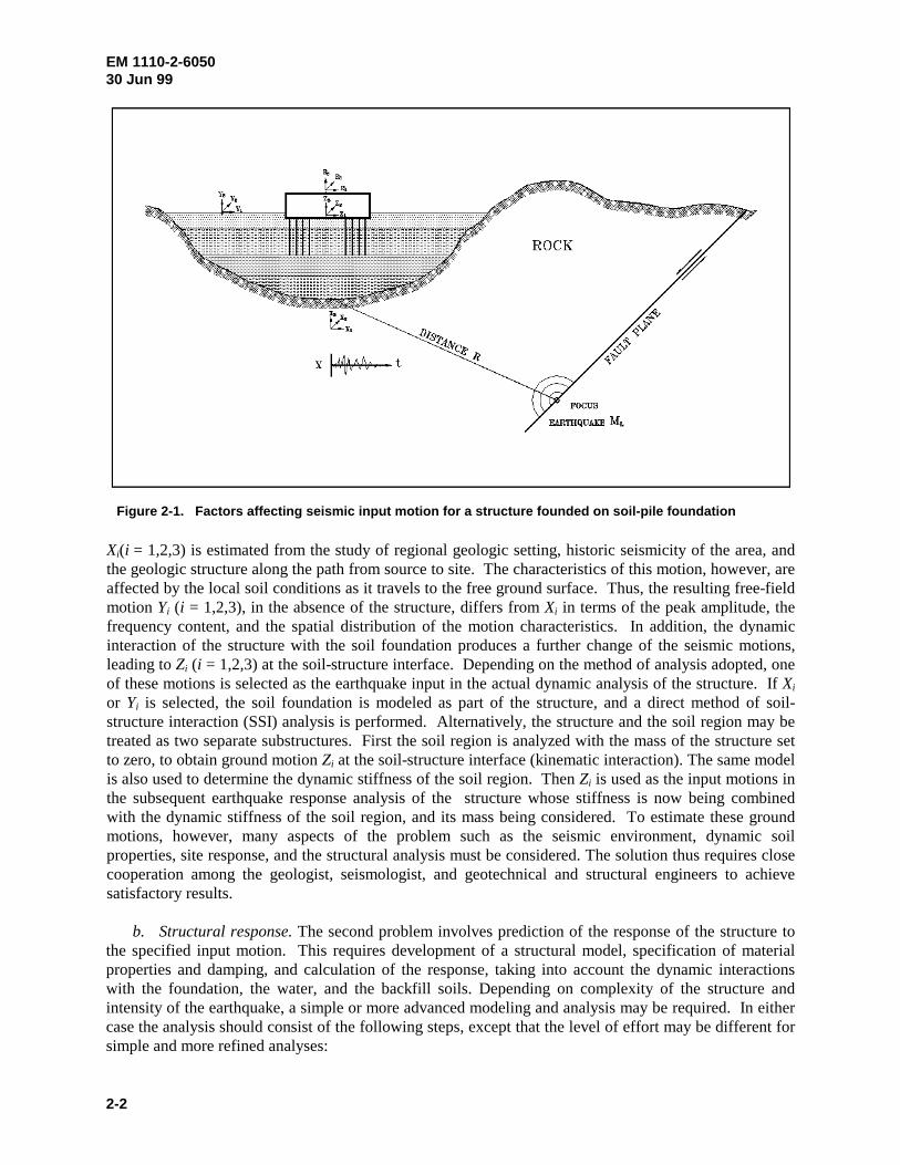
a. Input motion(s). A general description of the factors affecting the earthquake input motions to beused in the design and evaluation of structures is demonstrated in Figure 2-1. The base rock motion

EM 1110-2-605030 Jun 99

2-2

Xi(i = 1,2,3) is estimated from the study of regional geologic setting, historic seismicity of the area, andthe geologic structure along the path from source to site. The characteristics of this motion, however, areaffected by the local soil conditions as it travels to the free ground surface. Thus, the resulting free-fieldmotion Yi (i = 1,2,3), in the absence of the structure, differs from Xi in terms of the peak amplitude, thefrequency content, and the spatial distribution of the motion characteristics. In addition, the dynamicinteraction of the structure with the soil foundation produces a further change of the seismic motions,leading to Zi (i = 1,2,3) at the soil-structure interface. Depending on the method of analysis adopted, oneof these motions is selected as the earthquake input in the actual dynamic analysis of the structure. If Xi

or Yi is selected, the soil foundation is modeled as part of the structure, and a direct method of soil-structure interaction (SSI) analysis is performed. Alternatively, the structure and the soil region may betreated as two separate substructures. First the soil region is analyzed with the mass of the structure setto zero, to obtain ground motion Zi at the soil-structure interface (kinematic interaction). The same modelis also used to determine the dynamic stiffness of the soil region. Then Zi is used as the input motions inthe subsequent earthquake response analysis of the structure whose stiffness is now being combinedwith the dynamic stiffness of the soil region, and its mass being considered. To estimate these groundmotions, however, many aspects of the problem such as the seismic environment, dynamic soilproperties, site response, and the structural analysis must be considered. The solution thus requires closecooperation among the geologist, seismologist, and geotechnical and structural engineers to achievesatisfactory results.

b. Structural response. The second problem involves prediction of the response of the structure tothe specified input motion. This requires development of a structural model, specification of materialproperties and damping, and calculation of the response, taking into account the dynamic interactionswith the foundation, the water, and the backfill soils. Depending on complexity of the structure andintensity of the earthquake, a simple or more advanced modeling and analysis may be required. In eithercase the analysis should consist of the following steps, except that the level of effort may be different forsimple and more refined analyses:

Figure 2-1. Factors affecting seismic input motion for a structure founded on soil-pile foundation

EM 1110-2-605030 Jun 99

2-3

(1) Establishment of earthquake design criteria.

(2) Development of design earthquakes and associated ground motions.

(3) Establishment of analysis procedure.

(4) Development of structural models.

(5) Prediction of earthquake response of the structure.

(6) Interpretation and evaluation of results.

2-3. Design Criteria

The design and evaluation of hydraulic structures for earthquake loading must be based on appropriatecriteria that reflect both the desired level of safety and the choice of the design and evaluation procedures(ER 1110-2-1806). The first requirement is to establish design earthquake ground motions to be used asthe seismic input by giving due consideration to the consequences of failure and the designatedoperational function. Then the response of the structure to this seismic input must be calculated takinginto account the significant interactions with the rock, soil, or pile foundation as well as with theimpounded, or surrounding and contained water. The analysis should be formulated using a realisticidealization of the structure-water-foundation system, and the results are evaluated in view of thelimitations, assumptions, and uncertainties associated with the seismic input and the method of analysis.

2-4. Design Earthquakes

a. Operating basis earthquake (OBE).

(1) Definition and performance. The OBE is an earthquake that can reasonably be expected to occurwithin the service life of the project, that is, with a 50 percent probability of exceedance during theservice life. (This corresponds to a return period of 144 years for a project with a service life of100 years.) The associated performance requirement is that the project function with little or no damage,and without interruption of function. The purpose of the OBE is to protect against economic losses fromdamage or loss of service. Therefore alternative choices of return period for the OBE may be based oneconomic considerations. In a site-specific study the OBE is determined by a PSHA (ER 1110-2-1806).

(2) Analysis. For the OBE, the linear elastic analysis is adequate for computing seismic response ofthe structure, and the simple stress checks in which the predicted elastic stresses are compared with theexpected concrete strength should suffice for the performance evaluation. Structures located in regionsof high seismicity should essentially respond elastically to the OBE event with no disruption to service,but limited localized damage is permissible and should be repairable. In such cases, a low to moderatelevel of damage can be expected, but the results of a linear time-history analysis with engineeringjudgment may still be used to provide a reasonable estimate of the expected damage.

b. Maximum design earthquake (MDE).

(1) Definition and performance. The MDE is the maximum level of ground motion for which astructure is designed or evaluated. The associated performance requirement is that the project performswithout catastrophic failure, such as uncontrolled release of a reservoir, although severe damage oreconomic loss may be tolerated. The MDE can be characterized as a deterministic or probabilistic event(ER 1110-2-1806).

EM 1110-2-605030 Jun 99

2-4

(a) For critical structures the MDE is set equal to the MCE. Critical structures are defined inER 1110-2-1806 as structures of high downstream hazard whose failure during or immediately followingan earthquake could result in loss of life. The MCE is defined as the greatest earthquake that canreasonably be expected to be generated by a specific source on the basis of seismological and geologicalevidence (ER 1110-2-1806).

(b) For other than critical structures the MDE is selected as a lesser earthquake than the MCE, whichprovides for an economical design meeting specified safety standards. This lesser earthquake is chosenbased upon an appropriate probability of exceedance of ground motions during the design life of thestructure (also characterized as a return period for ground motion exceedance).

(2) Nonlinear response. The damage during an MDE event could be substantial, but it should not becatastrophic in terms of loss of life, economics, and social and environmental impacts. It is evident that arealistic design criterion for evaluation of the response to damaging MDEs should include nonlinearanalysis, which can predict the nature and the extent of damage. However, a complete and reliablenonlinear analysis that includes tensile cracking of concrete, yielding of reinforcements, opening ofjoints, and foundation failure is not currently practical. Only limited aspects of the nonlinear earthquakeresponse behavior of the mass concrete structures such as contraction joint opening in arch dams, tensilecracking in concrete gravity dams, and sliding of concrete monoliths have been investigated previously.There is a considerable lack of knowledge with respect to nonlinear response behavior of the hydraulicstructures. Any consideration of performing nonlinear analysis for hydraulic structures should be done inconsultation with CECW-ED.

(3) Performance evaluation. The earthquake performance evaluation of the response of hydraulicstructures to a damaging MDE is presently based on the results of linear elastic analysis. In many cases, alinear elastic analysis can provide a reasonable estimate of the level of expected damage when thecracking, yielding, or other forms of nonlinearity are considered to be slight to moderate.

(a) URC. For URC hydraulic structures subjected to a severe MDE, the evaluation of damage usingthe linear time-history analysis may still continue. The evaluation, however, must be based on a rationalinterpretation of the results by giving due consideration to several factors including number and durationof stress excursions beyond the allowable limits, the ratio of computed to allowable values, simultaneousstress distributions at critical time-steps, size and location of overstressed area, and engineeringjudgment.

(b) RC. Such evaluation for the RC hydraulic structures should include approximate postelasticanalysis of the system considering ductility and energy dissipation beyond yield. First the section forcesfor critical members are computed using the linear elastic analysis procedure described in this manual.These forces are defined as the force demands imposed on the structure by the earthquake. Next the yieldor plastic capacities at the same locations are computed and defined as the force capacities. Finally, theratio of force demands to force capacities is computed to establish the demand-capacity ratios for all theselected locations. The resulting demand-capacity ratios provide an indication of the ductility that maybe required for the structural members to withstand the MDE level of ground motion. If the computeddemand-capacity ratios for a particular structure exceed the limits set forth in the respective designdocuments for that structure, approximate postelastic analyses should be performed to ensure that theinelastic demands of the MDE excitation on the structure can be resisted by the supplied capacity. Thisevaluation consists of several equivalent linear analyses with revised stiffness or resistancecharacteristics of all structural members that have reached their yielding capacities. The stiffnessmodification and analysis of the modified structure are repeated until no further yielding will occur or thestructure reaches a limit state with excessive distortions, mechanism, or instability.

EM 1110-2-605030 Jun 99

2-5

2-5. Earthquake Ground Motions

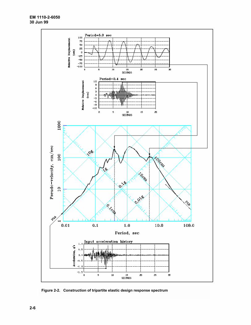
Earthquake ground motions for analysis of hydraulic structures are usually characterized by peak groundacceleration, response spectra, and acceleration time-histories. The peak ground acceleration (usually asa fraction of the peak) is the earthquake ground motion parameter usually used in the seismic coefficientmethod of analysis. The earthquake ground motions for dynamic analysis, as a minimum, should bespecified in terms of response spectra (Figure 2-2). A time-history earthquake response analysis, ifrequired, should be performed using the acceleration time-histories. The standard response spectra aredescribed in the following paragraphs, and procedures for estimating site-specific response spectra arediscussed in Chapter 3.

a. Elastic design response spectra. Elastic design response spectra of ground motions can bedefined by using standard or site-specific procedures. As illustrated in Figure 2-2, elastic designresponse spectra represent maximum responses of a series of single-degree-of-freedom (SDOF) systemsto a given ground motion excitation (Ebeling 1992; Chopra 1981; Clough and Penzien 1993; Newmarkand Rosenblueth 1971). The maximum displacements, maximum pseudo-velocities, and maximumpseudo-accelerations presented on a logarithmic tripartite graph provide advance insight into the dynamicbehavior of a structure. For example, Figure 2-2 shows that at low periods of vibration (<0.05 sec), thespectral or pseudo-accelerations approach the PGA, an indication that the rigid or very short periodstructures undergo the same accelerations as the ground. This figure also shows that structures withperiods in the range of about 0.06 to 0.5 sec are subjected to amplified accelerations and thus higherearthquake forces, whereas the earthquake forces for flexible structures with periods in the range ofabout 1 to 20 sec are reduced substantially but their maximum displacements exceed that of the ground.In the extreme, when the period exceeds 20 sec, the structure experiences the same maximumdisplacement as the ground. The response spectrum amplifications depend on the values of damping andare significantly influenced by the earthquake magnitude, source-to-site distance, and the site conditions(Chapter 3).

(1) Standard or normalized response spectra. The standard response spectra described in this sectionare to be used in accord with ER 1110-2-1806 and follow-up guidance. The development starts withthe spectral acceleration ordinates obtained from the National Earthquake Hazards ReductionProgram (NEHRP) hazard maps. The site coefficients to be used with the hazard maps todevelop standard response spectra for various soil profiles, as well as the methodology to constructresponse spectra at return periods other than those given in NEHRP, are provided in the guidance inER 1110-2-1806.

(2) Site-specific response spectra.

(a) Site-specific procedures to produce design response spectra are to be used in accord withER 1110-2-1806. Site-specific response spectra correspond to those expected on the basis of theseismological and geological calculations for the site. The procedures described in Chapter 3 use eitherthe deterministic or probabilistic method to develop site-specific spectra.

(b) While the deterministic method provides a single estimate of the peak ground acceleration andresponse spectral amplitudes, the probabilistic method estimates these parameters as a function ofprobability of exceedance or return period. To select the return period to use for the OBE and MDE, seethe definitions of these design earthquakes in paragraphs 2-4a and 2-4b, respectively. The resultingresponse spectra for the selected return period should then be used as input for quantifying the seismicloads required for the design and analysis of structures.

EM 1110-2-605030 Jun 99

2-6

Figure 2-2. Construction of tripartite elastic design response spectrum

EM 1110-2-605030 Jun 99

2-7

b. Acceleration time-histories. Various procedures for developing representative acceleration time-histories at a site are described in Chapter 3. Whenever possible, the acceleration time-histories shouldbe selected to be similar to the design earthquake in the following aspects: tectonic environment,earthquake magnitude, fault rupture mechanism (fault type), site conditions, design response spectra, andduration of strong shaking. Since it is not always possible to find records that satisfy all of these criteria,it is often necessary to modify existing records or develop synthetic records that meet most of theserequirements.

2-6. Establishment of Analysis Procedures

Seismic analysis of hydraulic structures should conform to the overall objectives of new designs andsatisfy the specific requirements of safety evaluation of existing structures. The choice of analysisprocedures may influence the scope and nature of the seismic input characterization, design procedures,specification of material properties, and evaluation and interpretation of the results. Simple proceduresrequire fewer and easily available parameters, while refined analyses usually need more comprehensivedefinition of the seismic input, structural idealization, and material properties. The analysis should beginwith the simplest procedures possible and then, if necessary, progress to more refined and advancedtypes. Simplified procedures are usually adequate for the feasibility and preliminary studies, whereasrefined procedures are more appropriate for the final design and safety evaluation of structures. Thesimplified analysis also serves to assess the need for a more elaborate analysis and provide a baseline forcomparison with the results obtained from the more elaborate analyses.

2-7. Structural Idealization

Structural models should be developed by giving careful consideration to the geometry, stiffness, andmass distributions, all of which affect the dynamic characteristics of the structure. The engineeringjudgment and knowledge of the dynamics of structures are required to develop a satisfactory model thatis both simple and representative of the most important dynamic behavior of the structure. Depending onits level of complexity, a hydraulic structure may be represented by a simplified one-dimensional model,a planar or 2-D model whose deformations are restricted in a plane, or by a more elaborate 3-D model toaccount for its 3-D behavior.

a. Simplified models. Structures with regular geometry and mass distribution along one axis may beidealized by simplified models using the beam theory. The simplified model should approximatelyrepresent the significant features of the dynamic response of the structure including the fundamentalperiod and mode shape, as well as the effects of structure-foundation and structure-water interaction.Two such simplified models have been developed for the free-standing intake towers and thenonoverflow gravity dam sections. In both cases, the simplified models were formulated based on theresults of finite element analyses that rigorously accounted for the structure-water-foundation interactioneffects, as well as for the reservoir bottom energy absorption for the gravity dams.

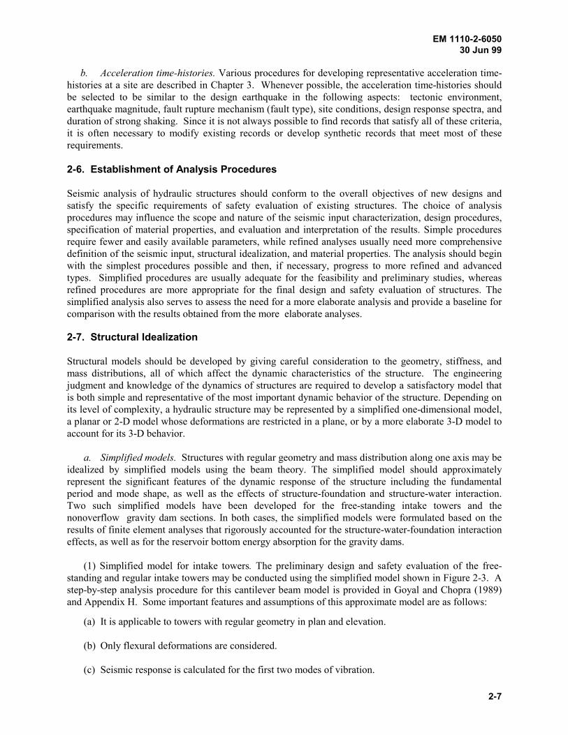
(1) Simplified model for intake towers. The preliminary design and safety evaluation of the free-standing and regular intake towers may be conducted using the simplified model shown in Figure 2-3. Astep-by-step analysis procedure for this cantilever beam model is provided in Goyal and Chopra (1989)and Appendix H. Some important features and assumptions of this approximate model are as follows:

(a) It is applicable to towers with regular geometry in plan and elevation.

(b) Only flexural deformations are considered.

(c) Seismic response is calculated for the first two modes of vibration.

EM 1110-2-605030 Jun 99

2-8

FIRSTMODE

ga (t)

1

2,3

4

12

LUMPED MASS

MODESECOND

(d) Foundation-structure interaction effects are considered only for the first mode of vibration.

(e) Interaction between the tower and the inside and outside water is represented by the added massassumption.

(f) The effects of vertical component of ground motion are ignored.

Note that slender towers with cross-section dimensions 10 times less than the height of the structure canusually be adequately represented solely by the flexural deformations of the tower. However, the effectsof shear deformations on vibration frequencies and section forces, especially for higher modes, aresignificant when the cross-section dimensions exceed 1/10 of the tower height and should be includedin the analysis. The effects of shear deformation can be incorporated in the analysis if a computerprogram with beam elements including shear deformation is used. The earthquake response for thissimplified model should be calculated for the combined effects of the two horizontal components of theground motions. The maximum shear forces, moments, and stresses for each lateral direction arecomputed separately using the specified response spectrum and the calculated vibration propertiesassociated with that direction. The total response values of the tower are then obtained by combining theresponses caused by each of the two components of the earthquake ground motion, as discussed inparagraph 2.8a(2)(f).

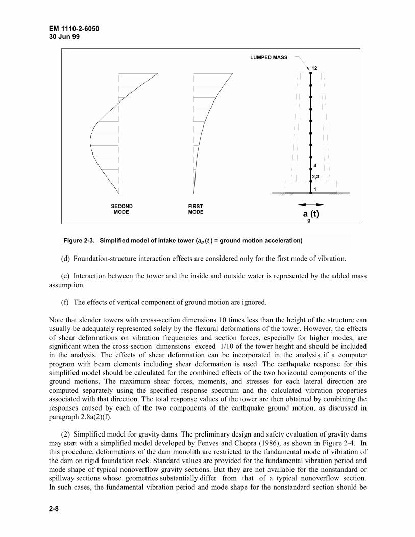
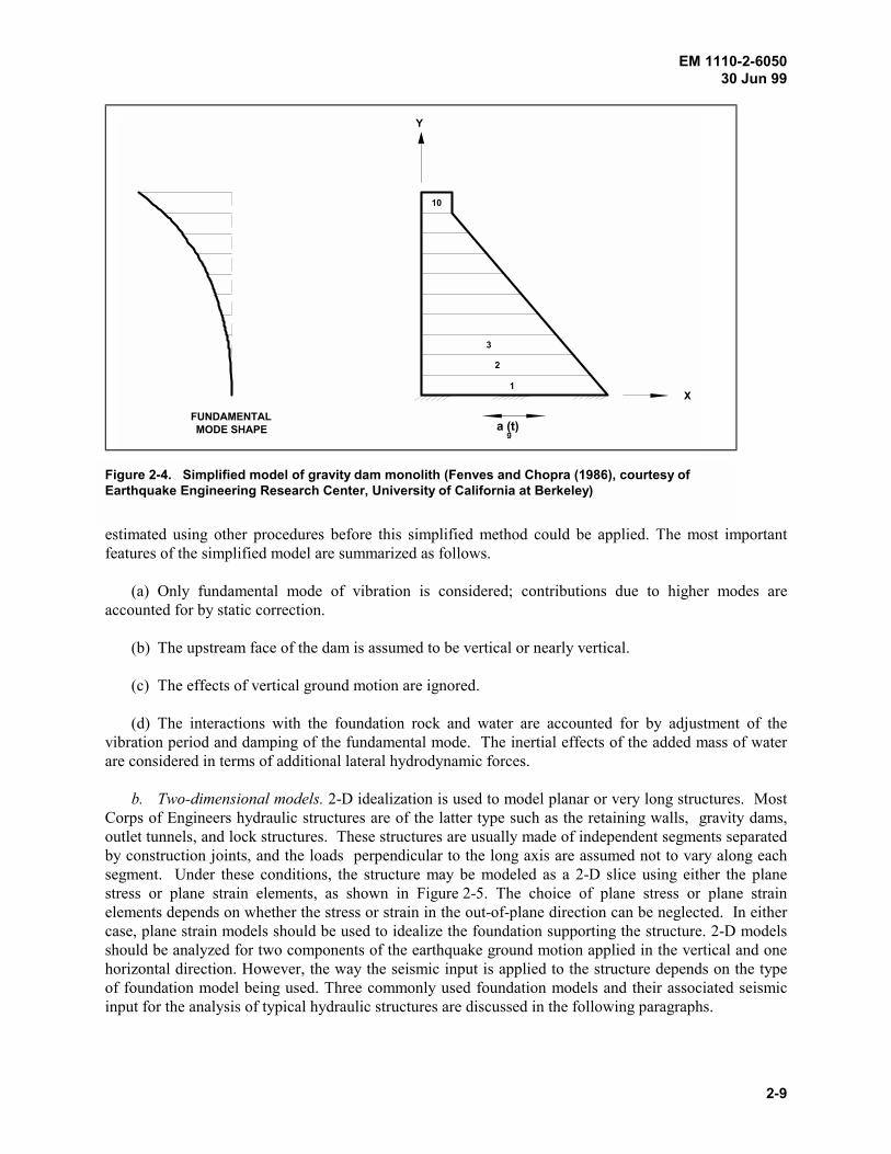
(2) Simplified model for gravity dams. The preliminary design and safety evaluation of gravity damsmay start with a simplified model developed by Fenves and Chopra (1986), as shown in Figure 2-4. Inthis procedure, deformations of the dam monolith are restricted to the fundamental mode of vibration ofthe dam on rigid foundation rock. Standard values are provided for the fundamental vibration period andmode shape of typical nonoverflow gravity sections. But they are not available for the nonstandard orspillway sections whose geometries substantially differ from that of a typical nonoverflow section.In such cases, the fundamental vibration period and mode shape for the nonstandard section should be

Figure 2-3. Simplified model of intake tower (ag (t ) = ground motion acceleration)

EM 1110-2-605030 Jun 99

2-9

X

Y

a (t)g

FUNDAMENTALMODE SHAPE

1

2

3

10

estimated using other procedures before this simplified method could be applied. The most importantfeatures of the simplified model are summarized as follows.

(a) Only fundamental mode of vibration is considered; contributions due to higher modes areaccounted for by static correction.

(b) The upstream face of the dam is assumed to be vertical or nearly vertical.

(c) The effects of vertical ground motion are ignored.

(d) The interactions with the foundation rock and water are accounted for by adjustment of thevibration period and damping of the fundamental mode. The inertial effects of the added mass of waterare considered in terms of additional lateral hydrodynamic forces.

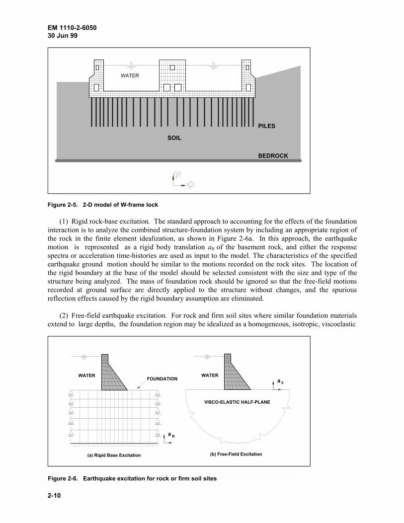
b. Two-dimensional models. 2-D idealization is used to model planar or very long structures. MostCorps of Engineers hydraulic structures are of the latter type such as the retaining walls, gravity dams,outlet tunnels, and lock structures. These structures are usually made of independent segments separatedby construction joints, and the loads perpendicular to the long axis are assumed not to vary along eachsegment. Under these conditions, the structure may be modeled as a 2-D slice using either the planestress or plane strain elements, as shown in Figure 2-5. The choice of plane stress or plane strainelements depends on whether the stress or strain in the out-of-plane direction can be neglected. In eithercase, plane strain models should be used to idealize the foundation supporting the structure. 2-D modelsshould be analyzed for two components of the earthquake ground motion applied in the vertical and onehorizontal direction. However, the way the seismic input is applied to the structure depends on the typeof foundation model being used. Three commonly used foundation models and their associated seismicinput for the analysis of typical hydraulic structures are discussed in the following paragraphs.

Figure 2-4. Simplified model of gravity dam monolith (Fenves and Chopra (1986), courtesy ofEarthquake Engineering Research Center, University of California at Berkeley)

EM 1110-2-605030 Jun 99

2-10

WATER

PILES

SOIL

BEDROCK

Figure 2-5. 2-D model of W-frame lock

(1) Rigid rock-base excitation. The standard approach to accounting for the effects of the foundationinteraction is to analyze the combined structure-foundation system by including an appropriate region ofthe rock in the finite element idealization, as shown in Figure 2-6a. In this approach, the earthquakemotion is represented as a rigid body translation aR of the basement rock, and either the responsespectra or acceleration time-histories are used as input to the model. The characteristics of the specifiedearthquake ground motion should be similar to the motions recorded on the rock sites. The location ofthe rigid boundary at the base of the model should be selected consistent with the size and type of thestructure being analyzed. The mass of foundation rock should be ignored so that the free-field motionsrecorded at ground surface are directly applied to the structure without changes, and the spuriousreflection effects caused by the rigid boundary assumption are eliminated.

(2) Free-field earthquake excitation. For rock and firm soil sites where similar foundation materialsextend to large depths, the foundation region may be idealized as a homogeneous, isotropic, viscoelastic

(a) Rigid Base Excitation (b) Free-Field Excitation

VISCO-ELASTIC HALF-PLANE

FOUNDATION a F

a R

WATER WATER

Figure 2-6. Earthquake excitation for rock or firm soil sites

EM 1110-2-605030 Jun 99

2-11

half-plane (Dasgupta and Chopra 1979), as shown in Figure 2-6b. In this case, the structure is supportedon the horizontal surface of the foundation, and the earthquake response is formulated with respect to thefree-field definition of the ground motion aF rather than the basement rock input. The interaction effectsof the foundation are represented by a frequency-dependent dynamic stiffness matrix defined withrespect to the degrees of freedom on the structure-foundation interface. The seismic input for thisidealization is in the form of acceleration time-histories of the free-field motion; the response spectrummethod of analysis is not applicable. This method is currently used in the analysis of gravity dams andfree-standing intake towers when the foundation material can be assumed homogeneous.

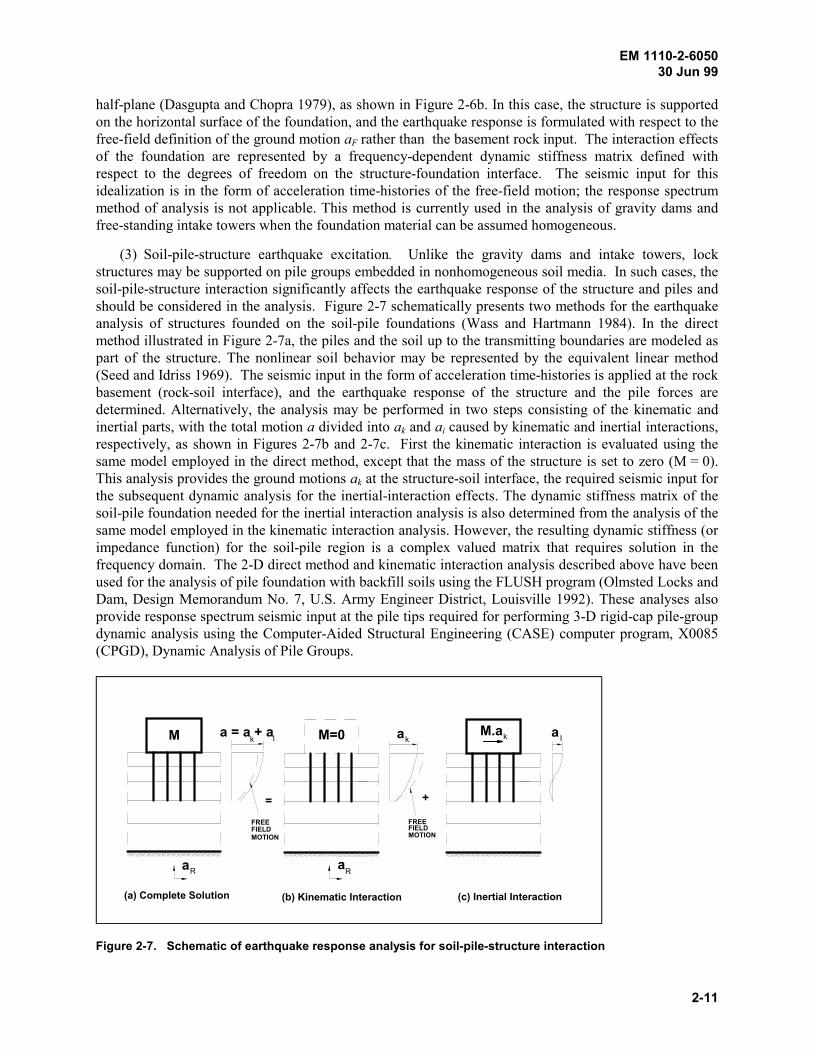
(3) Soil-pile-structure earthquake excitation. Unlike the gravity dams and intake towers, lockstructures may be supported on pile groups embedded in nonhomogeneous soil media. In such cases, thesoil-pile-structure interaction significantly affects the earthquake response of the structure and piles andshould be considered in the analysis. Figure 2-7 schematically presents two methods for the earthquakeanalysis of structures founded on the soil-pile foundations (Wass and Hartmann 1984). In the directmethod illustrated in Figure 2-7a, the piles and the soil up to the transmitting boundaries are modeled aspart of the structure. The nonlinear soil behavior may be represented by the equivalent linear method(Seed and Idriss 1969). The seismic input in the form of acceleration time-histories is applied at the rockbasement (rock-soil interface), and the earthquake response of the structure and the pile forces aredetermined. Alternatively, the analysis may be performed in two steps consisting of the kinematic andinertial parts, with the total motion a divided into ak and ai caused by kinematic and inertial interactions,respectively, as shown in Figures 2-7b and 2-7c. First the kinematic interaction is evaluated using thesame model employed in the direct method, except that the mass of the structure is set to zero (M = 0).This analysis provides the ground motions ak at the structure-soil interface, the required seismic input forthe subsequent dynamic analysis for the inertial-interaction effects. The dynamic stiffness matrix of thesoil-pile foundation needed for the inertial interaction analysis is also determined from the analysis of thesame model employed in the kinematic interaction analysis. However, the resulting dynamic stiffness (orimpedance function) for the soil-pile region is a complex valued matrix that requires solution in thefrequency domain. The 2-D direct method and kinematic interaction analysis described above have beenused for the analysis of pile foundation with backfill soils using the FLUSH program (Olmsted Locks andDam, Design Memorandum No. 7, U.S. Army Engineer District, Louisville 1992). These analyses alsoprovide response spectrum seismic input at the pile tips required for performing 3-D rigid-cap pile-groupdynamic analysis using the Computer-Aided Structural Engineering (CASE) computer program, X0085(CPGD), Dynamic Analysis of Pile Groups.

Ra

(a) Complete Solution (b) Kinematic Interaction (c) Inertial Interaction

M M=0

= +

M.aka = a + ak I ak

aR

a I

FREEFIELDMOTION

FREEFIELDMOTION

Figure 2-7. Schematic of earthquake response analysis for soil-pile-structure interaction

EM 1110-2-605030 Jun 99

2-12

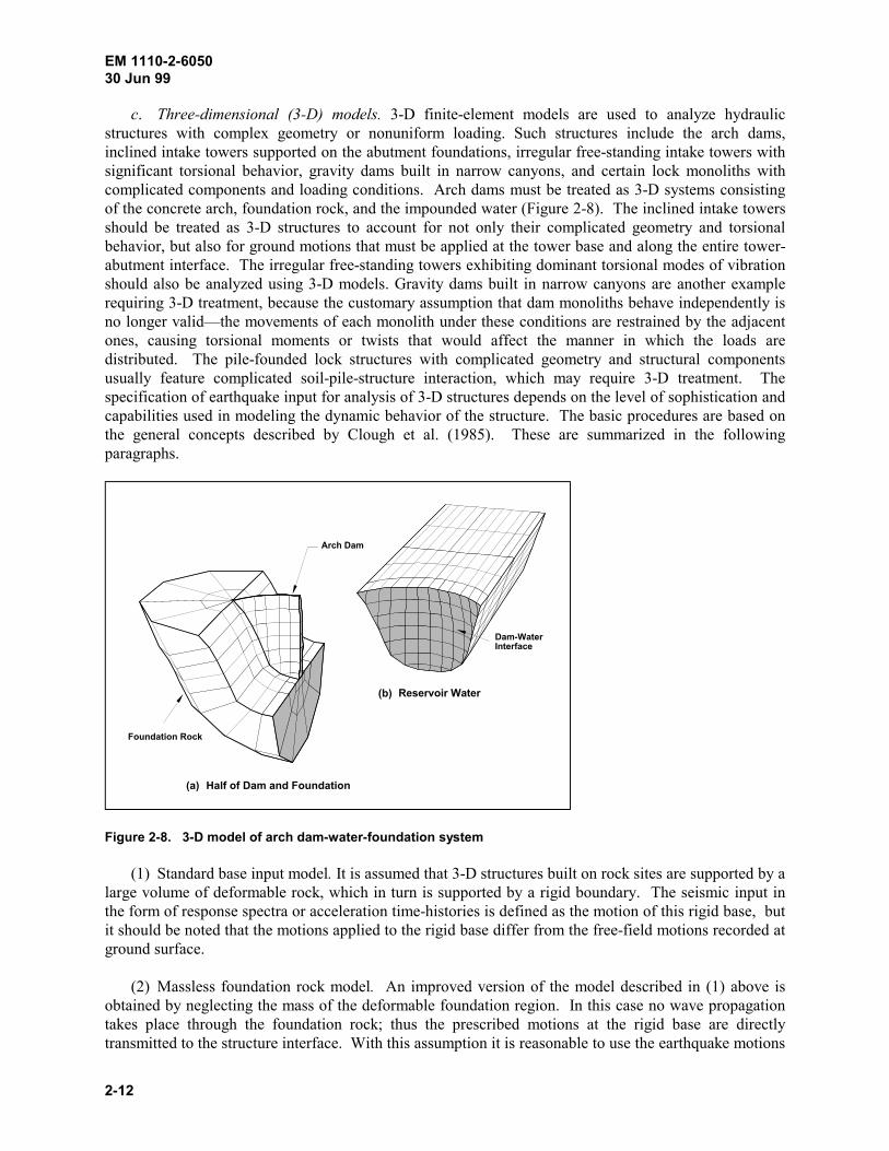
c. Three-dimensional (3-D) models. 3-D finite-element models are used to analyze hydraulicstructures with complex geometry or nonuniform loading. Such structures include the arch dams,inclined intake towers supported on the abutment foundations, irregular free-standing intake towers withsignificant torsional behavior, gravity dams built in narrow canyons, and certain lock monoliths withcomplicated components and loading conditions. Arch dams must be treated as 3-D systems consistingof the concrete arch, foundation rock, and the impounded water (Figure 2-8). The inclined intake towersshould be treated as 3-D structures to account for not only their complicated geometry and torsionalbehavior, but also for ground motions that must be applied at the tower base and along the entire tower-abutment interface. The irregular free-standing towers exhibiting dominant torsional modes of vibrationshould also be analyzed using 3-D models. Gravity dams built in narrow canyons are another examplerequiring 3-D treatment, because the customary assumption that dam monoliths behave independently isno longer valid—the movements of each monolith under these conditions are restrained by the adjacentones, causing torsional moments or twists that would affect the manner in which the loads aredistributed. The pile-founded lock structures with complicated geometry and structural componentsusually feature complicated soil-pile-structure interaction, which may require 3-D treatment. Thespecification of earthquake input for analysis of 3-D structures depends on the level of sophistication andcapabilities used in modeling the dynamic behavior of the structure. The basic procedures are based onthe general concepts described by Clough et al. (1985). These are summarized in the followingparagraphs.

Arch Dam

Foundation Rock

Dam-WaterInterface

Half of Dam and Foundation(a)

(b) Reservoir Water

Figure 2-8. 3-D model of arch dam-water-foundation system

(1) Standard base input model. It is assumed that 3-D structures built on rock sites are supported by alarge volume of deformable rock, which in turn is supported by a rigid boundary. The seismic input inthe form of response spectra or acceleration time-histories is defined as the motion of this rigid base, butit should be noted that the motions applied to the rigid base differ from the free-field motions recorded atground surface.

(2) Massless foundation rock model. An improved version of the model described in (1) above isobtained by neglecting the mass of the deformable foundation region. In this case no wave propagationtakes place through the foundation rock; thus the prescribed motions at the rigid base are directlytransmitted to the structure interface. With this assumption it is reasonable to use the earthquake motions

EM 1110-2-605030 Jun 99

2-13

recorded at the ground surface as the rigid base input as for the 2-D analysis in Figure 2-6a. Thisprocedure is commonly used in the practical analysis of 3-D structures built on rock sites. GDAP(Ghanaat 1993) and ADAP-88 (Fenves, Mojtahedi, and Reimer 1989) and other arch dam analysisprograms commonly use this type of foundation model.

(3) Deconvolution base rock input model. In this approach the recorded free-field surface motionsare deconvolved to determine the motions at the rigid base boundary. The deconvolution analysis isperformed on a horizontally uniform layer of deformable rock or soil deposits using the one-dimensionalwave propagation theory. For the soil sites, however, the strain-dependent nature of the nonlinear soilshould be considered. The resulting rigid base motion is then applied at the base of the 3-D foundation-structure system, in which the foundation model is assumed to have its normal mass as well as stiffnessproperties. This procedure permits the wave propagation in the foundation rock, but requires anextensive model for the foundation rock, which computationally is inefficient.

(4) Free-field input model. A more reasonable approach for defining the seismic input would be toapply the deconvolved rigid base motion to a foundation model without the structure in place and tocalculate the free-field motions at the interface positions, where the structure will be located. Theseinterface free-field motions would be used as input to the combined structure-foundation model, whichemploys a relatively smaller volume of the rock region. It should be noted that the resulting seismicinput at the interface varies spatially due to the scattering effects of canyon walls (in the case of archdams) in addition to the traveling wave effects that also take place in the relatively long structures, evenwhen the contact surface is flat. In either case, the computer program used should have capabilities topermit multiple support excitation. The application of this procedure has not yet evolved to practicalproblems.

(5) Soil-pile-structure interaction model. The seismic input for 3-D structures supported on pilefoundations may be evaluated using a 3-D extension of the procedure discussed in b(3) above. However,the soil-pile-structure interaction analysis should also consider the inclined propagating body and surfacewaves if the structure is relatively long and is located close to a potential seismic source, or if it issupported on a sediment-filled basin. In particular, long-period structures with natural periods in thepredominant range of surface waves should be examined for the seismic input that accounts for theeffects of surface waves. One limiting factor in such analyses is the maximum number of piles that canbe considered in the analysis of structures on a flexible base. For example a pile-founded lock structuremay include a monolith having more than 800 piles. 3-D soil-structure interaction analysis programs suchas SASSI (Lysmer et al. 1981) with pile groups analysis capability may not be able to handle such a largeproblem without some program modifications or structural modeling assumptions that could lead to areduced number of piles for the idealized monolith.

2-8. Dynamic Analysis Procedures

The idealized model of structures and the prescribed earthquake ground motions are used to estimate thedynamic response of structures to earthquakes. The dynamic analysis is performed using the responsespectrum or time-history method. The response spectrum method is usually a required first step in adynamic analysis for the design and evaluation of hydraulic structures. In many cases it suffices for thestructures located in low seismic hazard regions. It is also the preferred design tool, because themaximum response values for the design can be obtained directly from the earthquake responsespectrum. However, the response spectrum procedure is an approximate method for calculating only themaximum response values and is restricted to the linear elastic analysis. The time-history method, on theother hand, is applicable to both linear elastic and nonlinear response analyses and is used when the time-dependent response characteristics or the nonlinear behavior is important, as explained later.

EM 1110-2-605030 Jun 99

2-14

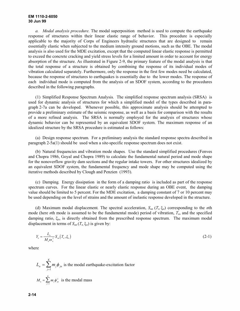
a. Modal analysis procedure. The modal superposition method is used to compute the earthquakeresponse of structures within their linear elastic range of behavior. This procedure is especiallyapplicable to the majority of Corps of Engineers hydraulic structures that are designed to remainessentially elastic when subjected to the medium intensity ground motions, such as the OBE. The modalanalysis is also used for the MDE excitation, except that the computed linear elastic response is permittedto exceed the concrete cracking and yield stress levels for a limited amount in order to account for energyabsorption of the structure. As illustrated in Figure 2-9, the primary feature of the modal analysis is thatthe total response of a structure is obtained by combining the response of its individual modes ofvibration calculated separately. Furthermore, only the response in the first few modes need be calculated,because the response of structures to earthquakes is essentially due to the lower modes. The response ofeach individual mode is computed from the analysis of an SDOF system, according to the proceduresdescribed in the following paragraphs.

(1) Simplified Response Spectrum Analysis. The simplified response spectrum analysis (SRSA) isused for dynamic analysis of structures for which a simplified model of the types described in para-graph 2-7a can be developed. Whenever possible, this approximate analysis should be attempted toprovide a preliminary estimate of the seismic response, as well as a basis for comparison with the resultsof a more refined analysis. The SRSA is normally employed for the analysis of structures whosedynamic behavior can be represented by an equivalent SDOF system. The maximum response of anidealized structure by the SRSA procedure is estimated as follows:

(a) Design response spectrum. For a preliminary analysis the standard response spectra described inparagraph 2-5a(1) should be used when a site-specific response spectrum does not exist.

(b) Natural frequencies and vibration mode shapes. Use the standard simplified procedures (Fenvesand Chopra 1986, Goyal and Chopra 1989) to calculate the fundamental natural period and mode shapefor the nonoverflow gravity dam sections and the regular intake towers. For other structures idealized byan equivalent SDOF system, the fundamental frequency and mode shape may be computed using theiterative methods described by Clough and Penzien (1993).

(c) Damping. Energy dissipation in the form of a damping ratio is included as part of the responsespectrum curves. For the linear elastic or nearly elastic response during an OBE event, the dampingvalue should be limited to 5 percent. For the MDE excitation, a damping constant of 7 or 10 percent maybe used depending on the level of strains and the amount of inelastic response developed in the structure.

(d) Maximum modal displacement. The spectral acceleration, San (Tn !n) corresponding to the nthmode (here nth mode is assumed to be the fundamental mode) period of vibration, Tn, and the specifieddamping ratio, !n, is directly obtained from the prescribed response spectrum. The maximum modaldisplacement in terms of San (Tn, !n) is given by:

" #YL

MS Tn

n

n n

an n n$%

!2

, (2-1)

where

L mn j jnj

K

$$& '

1

is the modal earthquake-excitation factor

M mn j jnj

K

$$& ' 2

1

is the modal mass

EM 1110-2-605030 Jun 99

2-15

RESPONSE SPECTRUM ANALYSIS

(1) Compute mode shapes [ ''''j1, ''''j2, ''''j3] and natural periods [T1, T2, T3]

T T T12

a2

S

S

S

PERIOD

SPECTRALACCELERATION

3

a1

a3

(2) Obtain spectral accelerations [Sa1, Sa2, Sa3] for all modes

L m M m

PF L M

YPF

S where n

n jn jj

n jn jj

n n n

nn

nan

$ $

$

$ ( $

$ $& &' '

%

1

32

1

3

21 2 3

;

, ,

(3) Compute modal participation factor PFn

and maximum modal response Yn

Figure 2-9. Illustration of response spectrum mode-superposition analysis (Continued)

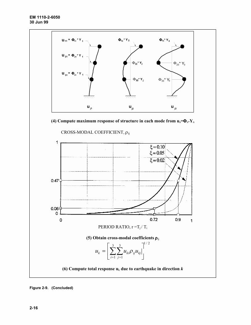
EM 1110-2-605030 Jun 99

2-16

)))) )))) ))))11 12 13* Y1

* Y21 1))))

)))) 1* Y

* Y 2 3* Yu11=

u u uj1

=21u

31u =

j2 j3

31

* Y)22

* Y)*+*+*+*+

)23* Y32

2 )33* Y3

(4) Compute maximum response of structure in each mode from un=))))n*Yn

CROSS-MODAL COEFFICIENT, ,ij

PERIOD RATIO, r =Tj / Ti

(5) Obtain cross-modal coefficients ,,,,ij

2/13

1

3

1-.

/01

2$ &&

$ $i jkjijkik uuu ,

(6) Compute total response uk due to earthquake in direction k

Figure 2-9. (Concluded)

EM 1110-2-605030 Jun 99

2-17

%n = 23/Tn is the circular frequency

K = number of degrees of freedom in structural model

The ratio Ln/Mn is the modal participation factor PFn indicating the degree to which mode n is excited bythe ground motion.

(e) Maximum displacement. With the maximum modal displacement being computed in step (d),the maximum displacement of the structure is computed as

" #uL

MS Tjn

n

njn an n n$

%' !2 , (2-2)

where 'jn is the assumed or calculated mode shape of the structure.

(f) Maximum shear and moment. The shear forces and moments at sections along the height of thestructure are obtained by static analysis from the equivalent lateral forces as follows:

" #nnanjnjn

njn TSm

M

Lf !' ,$ (2-3)

&$ jnn fV (2-4)

&$ jnjn fhM (2-5)

where

f jn = maximum value of equivalent lateral force at the jth section

hj = associated moment arm

(2) Response spectrum modal superposition method. The estimation of maximum response of ahydraulic structure to earthquake excitation usually involves many modes of vibration, which maycontribute significantly to the response. The contributions of various modes to the total displacements,forces, and stresses depend on a number of factors including the response spectrum ordinates, naturalperiods of vibration, and mode shapes, which in turn depend on the mass and stiffness properties of thestructure. The seismic responses of such structures are further complicated by the dynamic interactionwith the foundation supporting the structure and the impounded water. In general, the simplified SDOFprocedures described above may not be applicable in most cases or may provide only a very crudeestimate of the response. In these situations, the structure is analyzed using the response-spectrum modal-superposition method illustrated in Figure 2-9. The response-spectrum modal-superposition analysis isusually carried by standard or specialized programs following the same analysis steps described in a(1),but additional factors including the number of modes, combination of modal responses, and the effects ofmultiple components of earthquake input should also be considered.

(a) Number of modes. There are no guidelines for determining in advance how many modes shouldbe included in a response spectrum analysis, because it depends on the dynamic characteristics of thestructure and the response spectrum ordinates. However, the analysis should include a sufficient number

EM 1110-2-605030 Jun 99

2-18

of modes until the calculated response quantities are at least within 10 percent of the “exact” values.Since the “exact” response values are not known, a trial and error procedure may be adapted, in whichanalyses are repeated with addition of modes until it is seen that the addition of modes does notsignificantly affect the results. Alternatively, it may be demonstrated that the participating effectivemodal masses are at least within 90 percent of the total mass of the structures.

(b) Combination of modal responses. The response spectrum analysis procedure described aboveprovides only the maximum response in each mode of vibration. The response quantities of interest, suchas the peak displacements, element stresses, element forces, and moments, evaluated for each significantmode of vibration should be combined to obtain the total response of the structure. Since modalresponses do not occur at the same time during the earthquake excitation, they should be combined usingthe complete quadratic combination (CQC) or the square root of the sum of the squares (SRSS) methoddescribed below.

(c) CQC method. The CQC modal combination method (Wilson, Der Kiureghian, and Bayo 1981) isbased on random vibration theory and can be used in the response spectrum analysis if the duration of thestrong motion portion of the earthquake shaking is several times longer than the fundamental period ofthe structure and if the design response spectrum ordinates vary slowly over a wide range of periods thatinclude the dominant modes of the structure. Both conditions are easily met for short-period hydraulicstructures and smooth design response spectra with 5 percent damping or more. The CQC formula forthe maximum combined displacements uk to an earthquake in direction k is given by

1/2

1 1 --.

/

001

2,$ &&

$ $

N

i

N

jkjijkik uuu (2-6)

where uki and ukj are the maximum modal displacements corresponding to the vibration modes i and j,respectively, and N is the number of modes. The cross-modal coefficients ,ij for the above twoconditions and for the constant modal damping ! are expressed by

2222

232

141

18

)r(r)r(

r)r( /

ij 4!454!

$, (2-7)

where r is the ratio of natural period of jth mode, Tj, to the natural period of the ith mode, Ti. As illustratedin Figure 2-9, this equation indicates a significant interaction between closely spaced modes, especiallyat high damping values.

(d) SRSS method. For the structures for which the modal periods are well separated, ,ij approacheszero (for i 6 j), and the CQC method degenerates into the familiar SRSS method. The maximum totalresponse for a single earthquake response spectrum in direction k is then given by

21

1

2

/N

ikik uu -.

/01

2$ &

$

(2-8)

The SRSS method leads to conservative results for the well-separated vibration modes, but is inappropri-ate when they are closely spaced, because it ignores the contribution due to the cross-modal terms.

EM 1110-2-605030 Jun 99

2-19

(e) Calculation of section forces and moments. The output of most computer response-spectrumanalyses usually includes nodal displacements and element stresses only. The section forces andmoments required for the design of structures are not readily available, except when beam elements areused to idealize the structure. For nonbeam elements, the combined maximum stress values have no sign,and thus evaluation of section forces from these stresses, if not interpreted properly, may lead toincorrect results. Like the element stresses, section forces and moments should first be evaluated for theindividual modes and then combined by the CQC or SRSS method to obtain the maximum shears,thrusts, and moments at a specified cross section.

(f) Combining for multicomponent earthquake input. Three-dimensional structures are analyzed forthree orthogonal components of the earthquake ground motions applied in two horizontal and verticaldirection. The maximum response quantity of interest due to each component of the earthquake groundmotion is estimated separately as described above. The maximum responses due to all threecomponents of the earthquake ground motion are then combined according to the SRSS method:

213

1

2

/

kkuu--.

/

001

2$ &

$

(2-9)

The SRSS combination of the multicomponent earthquake responses can be used with either the SRSSor CQC modal combination method. With the SRSS modal combination, the summation for multi-component input can be performed before or after combination of the modal responses, but with theCQC method it should always be applied after the modal responses have been combined. Regular intaketowers with a circular or rectangular cross section are usually analyzed for two horizontal components ofthe ground motion and not the vertical. For such towers in addition to the SRSS method, the peak valueof any resultant response quantity due to the combined gravity and two horizontal components of groundmotion may also be obtained from the largest of the values given by the following equations:

yx RRRR 788$ 0 (2-10)

yx RRRR 878$ 0 (2-11)

where Rx is the peak response due to the x-component; Ry the y-component of horizontal ground motion;and R0, gravity loads. Equations 2-10 and 2-11 are usually used in conjunction with the standard responsespectra, and the SRSS method is employed with the site-specific response spectra. The value of 7 forcircular towers is taken equal to 0.40 and for rectangular towers equal to 0.3.

(g) Interpretation of analysis results. The basic results of response spectrum analysis consist of themaximum nodal displacements and element stresses (or forces). As discussed previously, these maximumresponses are estimated by combining responses from individual modes and multicomponent input. Theresulting dynamic responses obtained in this manner have no sign and may be interpreted as positive ornegative. For example, the maximum element dynamic stresses 9d are assumed to be either tension(positive) or compression (negative). Furthermore, the maximum values associated with each responsequantity are not concurrent and usually occur at different instants of time. Thus static equilibrium checkscannot be performed to validate the results. Most computer programs used to perform response spectrumanalysis do not compute section thrusts, shears, and moments for elements other than beam elements.To obtain section moments and forces from the computed stress results, the analyst should assign stresssigns that would produce the correct stress distribution across a specified section. This is done by a care-ful examination of the shape of the predominant response modes, from which the actual deflected shape

EM 1110-2-605030 Jun 99

2-20

of a member and the associated stress distributions can be predicted. As discussed previously, a betterapproach is first to compute modal section forces and moments from the modal stresses, and thencombine them using the CQC or SRSS method.

(h) Combining static and dynamic stresses. For the evaluation of earthquake performance ofhydraulic structures, the response-spectrum estimate of the dynamic stresses 9d should be combined withthe effects of the static loads 9s. Since response spectrum stresses have no sign, combination of static anddynamic stresses should consider dynamic stresses to be either positive or negative, leading to themaximum values of the total tensile or compressive stresses:

dsmax 989$9 (2-12)

It should be noted that only the similarly oriented components of 9s and 9d can be combined.

(3) Time-history method. The linear response of structures to earthquakes can also be computedusing the time-history method of analysis. In the time-history analysis normally the acceleration time-histories are used as the seismic input. Procedures for developing acceleration time-history input consis-tent with the design response spectrum are described in Chapter 3. The idealized structural models usedin the time-history analysis are essentially identical to those described previously for the response spec-trum analysis. The response history is computed using a step-by-step numerical integration procedureapplied either to the original equations of motion (direct method) or to the transformed equations inmodal coordinates (mode superposition) (Bathe and Wilson 1976). In the more efficient modesuperposition approach, first the response history for each mode is evaluated at each integration time-step, and then the modal response histories for all significant modes of vibration are combined todetermine the dynamic response of the structure.

(4) Need for time-history analysis. Linear time-history analysis is required when the results ofresponse spectrum analysis indicate that the computed maximum total stresses (or forces) exceed theallowable values, or when special conditions exist. The time-history analysis is performed to estimatethe deformations and stresses (or forces) more accurately by considering the time-dependent nature of thedynamic response to earthquake motions. The results of such analysis serve to demonstrate the generalbehavior of the dynamic response, and combined with rational interpretation and judgment can provide apreliminary estimate of the level of inelastic behavior. Most Corps hydraulic structures are designedessentially to respond within their linear range when subjected to low to moderate intensity earthquakes.For this level of ground motions, the linear time-history analysis provides satisfactory results. For majorearthquakes it is probable that the elastic capacity of the mass concrete would be exceeded, and somecracking and crushing of the concrete and yielding of reinforcing steels could occur. Prediction of theactual response and estimation of the expected damage and inelastic behavior under severe earthquakescan be evaluated only using a more complicated nonlinear analysis. However, linear analysis can still bevery valuable for a preliminary assessment of the damage and the level of postelastic response and canhelp to decide whether a nonlinear analysis should be performed. As part of this evaluation, the resultsof linear analysis for the URC hydraulic structures should be examined in a systematic manner to identifythe extent of overstressed regions at any particular point in time, to produce plots showing time-historiesof stresses and other response quantities of interest, and to determine statistics on the number of stresscycles exceeding the allowable values and the corresponding excursions of these stress cycles beyond thespecified limits.

b. Nonlinear time-history.

(1) Need for nonlinear analysis. A nonlinear time-history analysis may be necessary when the resultsof a linear analysis show that the structure could suffer significant damage during a major earthquake.

EM 1110-2-605030 Jun 99

2-21

Minor local damages have little effect on the overall integrity of the structure and can still be evaluatedby proper interpretation of the results of linear analysis. However, when the calculated tensile stresses(or forces) are significantly greater than the tensile strength of the concrete (or section capacity) over alarge region and are repeated several times during the earthquake excitation, severe cracking of theconcrete, joint slippage, and yielding of reinforcements can be expected. Under these conditions, thedynamic behavior of the structure is drastically different from the linear response, and a valid estimate ofthe damage is possible only if a true nonlinear performance is incorporated in the analysis.

(2) Realistic nonlinear analysis. A reasonable nonlinear analysis should take into account allsources of nonlinearity that contribute significantly to the nonlinear response behavior. The damagecaused by earthquake shaking is normally associated with significant loss in the structural stiffnessresulting from the concrete cracking, yielding of steel, opening of construction joints, slippage across theconstruction joints or cracking planes, and the nonlinear material behavior. Additional sources ofnonlinearity arise from the nonlinear soil and the fractured foundation rock supporting the structure, aswell as the separation of the structure and the foundation at the contact surface. At the present time,analytical techniques for a complete nonlinear earthquake analysis of hydraulic structures, including theinteraction with foundation and water, are not available. Only limited aspects of the nonlinear behaviorsuch as the contraction joint opening in arch dams, tensile cracking of gravity dams, sliding of blocks,and approximate postelastic analyses have been considered in practice. A realistic nonlinear analysis forthe seismic safety evaluation of hydraulic structures depends on a great deal of new developments in thefollowing topics: definition of seismic input, identification and specification of significant nonlinearmechanisms (joint opening and sliding, tensile cracking of the concrete, yielding and slippage ofreinforcing steel, nonlinear material behavior under cyclic loads, etc.), development of idealized modelsrepresenting the nonlinear behavior, numerical techniques and solution strategies for computing thenonlinear response, and development of criteria for acceptable performance and identification of possiblemodes of failure. The seismic input for a nonlinear analysis is in the form of acceleration time-histories.The key issues in developing time-histories for nonlinear analysis are duration of strong shaking, energyand pulse sequencing, special near-fault characteristics such as the source “fling,” and the number of setsof time-histories required for the analysis. The main difficulty in effective nonlinear analysis at thepresent is the lack of or limited knowledge on the actual nonlinear material properties of the mass andreinforced concrete under cyclic loading.

2-9. Sliding and Rotational Stability During Earthquakes

a. Sliding stability. The sliding stability evaluation of hydraulic structures under earthquakeloading can be made according to the traditional static equilibrium (seismic coefficient) and permanentdisplacement approaches described in Ebeling and Morrison (1992). In the traditional approach, thesliding stability is expressed in terms of a prescribed factor of safety against sliding, whereas in thepermanent displacement approach the structure is permitted to slide along its base but the accumulateddisplacement during the ground shaking should be limited to a specified allowable value.

(1) Seismic coefficient approach. In the seismic coefficient approach, the safety against sliding isdetermined on the basis of shear-friction factor of safety (Ebeling and Morrison 1992). The shear-frictionfactor of safety is defined as the ratio of the resisting to driving forces along a potential failure surface

" #FS

CA N U

V$

4 5&&&

tan' (2-13)

where

C = unit cohesion

A = area of base

EM 1110-2-605030 Jun 99

2-22

N& = summation of normal forces

U& = summation of uplift forces

tan ' = coefficient of internal friction

V& = summation of shear or driving forces

(a) The driving forces acting on the structure include the static and seismic inertia forces due toweight of the structure and to hydrodynamic pressures. Treating the system above the failure surface as arigid block, the inertia force associated with the mass of the structure is computed as the product of theseismic coefficient, as specified in ER 1110-2-1806, and the weight of the block. Similarly, the productof the seismic coefficient and the added mass of water moving with the structure produces inertia forcedue to the hydrodynamic pressure. The added mass of water may be computed using the Westergaardmethod (Westergaard 1933) or the equation given by Chopra (Chopra 1967):

Ma = 0.54,h2 (2-14)

where , is the density and h is the depth of water. The motion of the structure relative to the failuresurface is resisted by the shear strength mobilized between the structure and the surface by the frictionand cohesion, as shown in Equation 2-13. For example, the shear friction factor of safety for sliding ofthe gravity dam shown in Figure 2-10 is given by

ag

WHH

)UW(CAFS

ds ::;

<==>

?448

'54$

tan (2-15)

where

W = weight of dam

Hs = hydrostatic force

Hd = hydrodynamic force (i.e., Ma . a)

g = gravitational acceleration

a = ground motion acceleration or some fraction thereof

The 8 sign is for sliding in the downstream or upstream direction with the plus sign indicatingdownstream.

(b) When the earthquake forces are included in the sliding stability analysis, the calculated factor ofsafety against sliding may become less than one. A factor of safety of less than one indicates a transientsliding. The sliding is assumed to occur for as long as the ground acceleration is greater than the criticalvalue required for the driving force to exceed the resistance. However, due to the oscillatory nature of theearthquake ground motion, the sliding displacement is expected to be limited but could lead to excessivepermanent displacements.

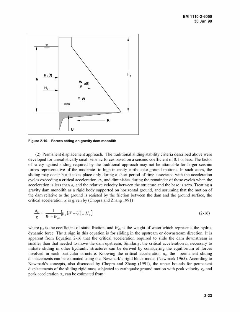
EM 1110-2-605030 Jun 99

2-23

Figure 2-10. Forces acting on gravity dam monolith

(2) Permanent displacement approach. The traditional sliding stability criteria described above weredeveloped for unrealistically small seismic forces based on a seismic coefficient of 0.1 or less. The factorof safety against sliding required by the traditional approach may not be attainable for larger seismicforces representative of the moderate- to high-intensity earthquake ground motions. In such cases, thesliding may occur but it takes place only during a short period of time associated with the accelerationcycles exceeding a critical acceleration, ac, and diminishes during the remainder of these cycles when theacceleration is less than ac and the relative velocity between the structure and the base is zero. Treating agravity dam monolith as a rigid body supported on horizontal ground, and assuming that the motion ofthe dam relative to the ground is resisted by the friction between the dam and the ground surface, thecritical acceleration ac is given by (Chopra and Zhang 1991)

" #@ Assa

c HUWWWg

a85B

4$

0

1 (2-16)

where Bs is the coefficient of static friction, and Wa0 is the weight of water which represents the hydro-dynamic force. The 8 sign in this equation is for sliding in the upstream or downstream direction. It isapparent from Equation 2-16 that the critical acceleration required to slide the dam downstream issmaller than that needed to move the dam upstream. Similarly, the critical acceleration ac necessary toinitiate sliding in other hydraulic structures can be derived by considering the equilibrium of forcesinvolved in each particular structure. Knowing the critical acceleration ac, the permanent slidingdisplacements can be estimated using the Newmark’s rigid block model (Newmark 1965). According toNewmark's concepts, also discussed by Chopra and Zhang (1991), the upper bounds for permanentdisplacements of the sliding rigid mass subjected to earthquake ground motion with peak velocity vm andpeak acceleration am can be estimated from :

hh

H

Wg

a(t)

W

U

R

d

s

dH (t)

DRAIN

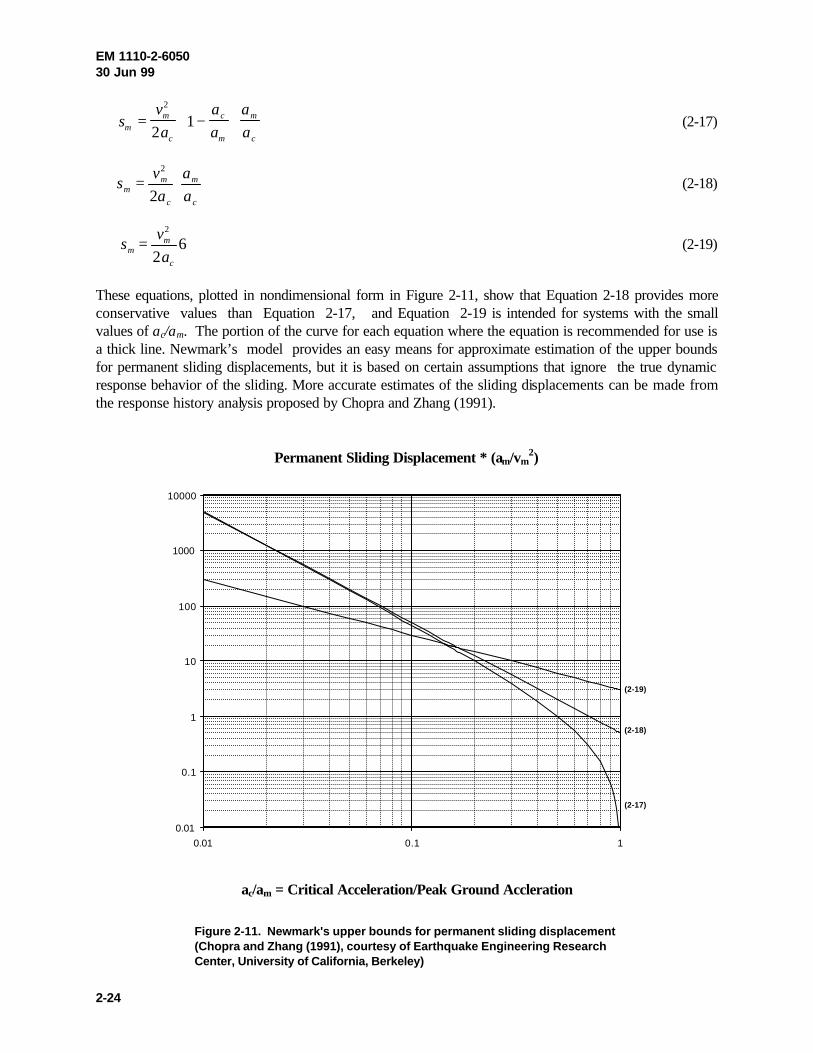
EM 1110-2-605030 Jun 99

2-24

sv

a

a

a

a

amm

c

c

m

m

c

= −

2

21 (2-17)

sv

a

a

amm

c

m

c

= ⋅2

2 (2-18)

sv

amm

c

=2

26 (2-19)

These equations, plotted in nondimensional form in Figure 2-11, show that Equation 2-18 provides moreconservative values than Equation 2-17, and Equation 2-19 is intended for systems with the smallvalues of ac/am. The portion of the curve for each equation where the equation is recommended for use isa thick line. Newmark’s model provides an easy means for approximate estimation of the upper boundsfor permanent sliding displacements, but it is based on certain assumptions that ignore the true dynamicresponse behavior of the sliding. More accurate estimates of the sliding displacements can be made fromthe response history analysis proposed by Chopra and Zhang (1991).

Permanent Sliding Displacement * (am/vm2)

ac/am = Critical Acceleration/Peak Ground Accleration

Figure 2-11. Newmark's upper bounds for permanent sliding displacement (Chopra and Zhang (1991), courtesy of Earthquake Engineering Research Center, University of California, Berkeley)

0.01

0.1

1

10

100

1000

10000

0.01 0.1 1

(2-19)

(2-18)

(2-17)

EM 1110-2-605030 Jun 99

2-25

b. Rotational stability. Hydraulic structures subjected to large lateral forces produced by majorearthquakes may tip and start rocking when the resulting overturning moment becomes so large that thestructure breaks contact with the ground.

(1) Intake towers. For an intake tower idealized as a nearly rigid or flexible equivalent SDOF system(Figure 2-12), the tipping occurs when the overturning moment exceeds the resisting moment due to theweight of the structure. This condition is expressed by:

mSah > mgb (2-20)

Sa > g (b/h) (2-21)

where

m = mass of structure

Sa = spectral acceleration of the earthquake ground motion

h = one-half height of structure

b = one-half base width of structure

Similar expressions can also be derived for other hydraulic structures, except that the moments due tohydrostatic and hydrodynamic forces should be included ((2) below). In both cases it is assumed that thestructure is not bonded to the ground, but it may be keyed into the soil with no pulling resistance. Itshould be noted that the structure will eventually overturn if the moment M > mgb is applied andsustained, where mgb represents the resisting moment due to the weight of the structure. However, underearthquake excitation large overturning moments occur for only a fraction of a second in each cycle,with intermediate opportunities to unload. By comparing the earthquake average energy input with therequired average energy for overturning the structure, Housner provided the following relationship as acriterion for the rotational stability of a rocking structure (Housner 1963):

0

v gI

mrS$7 (2-22)

where

7 = an angle defined in Figure 2-12

Sv = spectral velocity of the earthquake ground motion

m = mass of structure

r = radial distance from the center of gravity to tipping edge

I0 = moment inertia about the corner

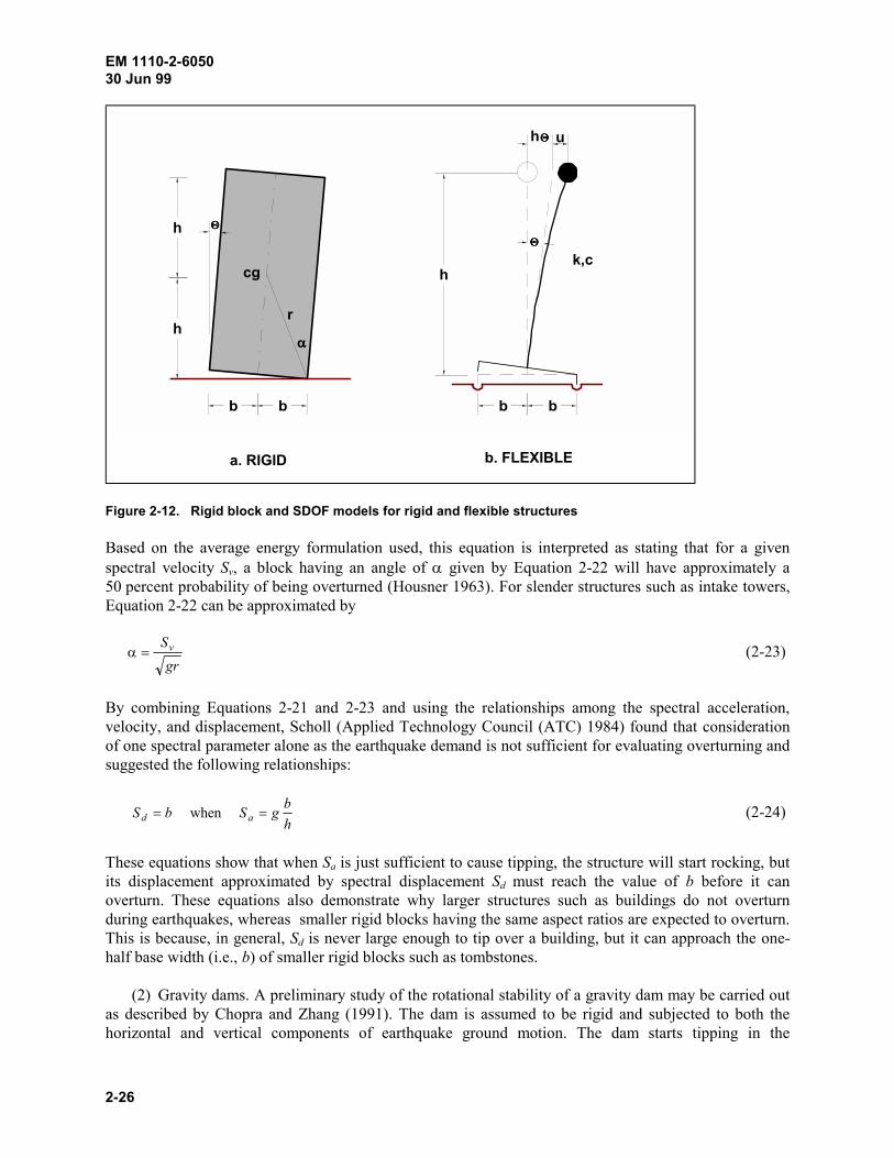
EM 1110-2-605030 Jun 99

2-26

cg

CCCC u

k,c

CCCC

7777h

h

bbbb

h

CCCC

a. RIGID b. FLEXIBLE

h

r

Figure 2-12. Rigid block and SDOF models for rigid and flexible structures

Based on the average energy formulation used, this equation is interpreted as stating that for a givenspectral velocity Sv, a block having an angle of 7 given by Equation 2-22 will have approximately a50 percent probability of being overturned (Housner 1963). For slender structures such as intake towers,Equation 2-22 can be approximated by

gr

Sv$7 (2-23)

By combining Equations 2-21 and 2-23 and using the relationships among the spectral acceleration,velocity, and displacement, Scholl (Applied Technology Council (ATC) 1984) found that considerationof one spectral parameter alone as the earthquake demand is not sufficient for evaluating overturning andsuggested the following relationships:

h

bgSbS ad $$ when (2-24)

These equations show that when Sa is just sufficient to cause tipping, the structure will start rocking, butits displacement approximated by spectral displacement Sd must reach the value of b before it canoverturn. These equations also demonstrate why larger structures such as buildings do not overturnduring earthquakes, whereas smaller rigid blocks having the same aspect ratios are expected to overturn.This is because, in general, Sd is never large enough to tip over a building, but it can approach the one-half base width (i.e., b) of smaller rigid blocks such as tombstones.

(2) Gravity dams. A preliminary study of the rotational stability of a gravity dam may be carried outas described by Chopra and Zhang (1991). The dam is assumed to be rigid and subjected to both thehorizontal and vertical components of earthquake ground motion. The dam starts tipping in the

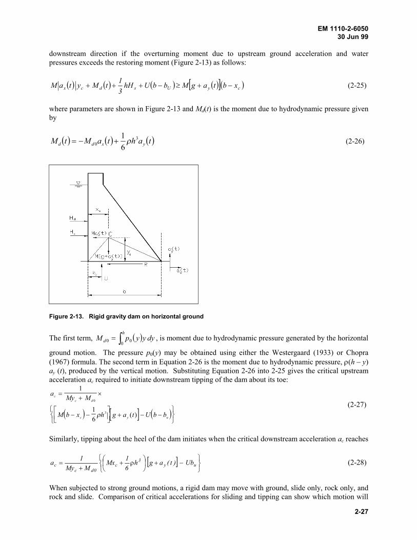
EM 1110-2-605030 Jun 99

2-27

downstream direction if the overturning moment due to upstream ground acceleration and waterpressures exceeds the restoring moment (Figure 2-13) as follows:

" # " # " # " #@ A" #cyUsdcx xbtagMbbUhH3

1tMytaM 54D5444 (2-25)

where parameters are shown in Figure 2-13 and Md(t) is the moment due to hydrodynamic pressure givenby

" # " # " #tahtaMtM yxdd3

0 6

1,45$ (2-26)

Figure 2-13. Rigid gravity dam on horizontal ground

The first term, " # dyyypMh

d E$ 000 , is moment due to hydrodynamic pressure generated by the horizontal

ground motion. The pressure p0(y) may be obtained using either the Westergaard (1933) or Chopra(1967) formula. The second term in Equation 2-26 is the moment due to hydrodynamic pressure, ,(h – y)ay (t), produced by the vertical motion. Substituting Equation 2-26 into 2-25 gives the critical upstreamacceleration ac required to initiate downstream tipping of the dam about its toe:

" # @ A " #

aMy M

M b x h g a t U b b

cc d

c y u

$4

F

5 5210

/.-

4 5 5GHI

JKL

1

1

6

0

3, ( )

(2-27)

Similarly, tipping about the heel of the dam initiates when the critical downstream acceleration ac reaches

@ ALKJ

IHG

54:;<

=>? ,4

4$ uy

3c

0dcc Ub)t(agh

6

1Mx

MMy

1a (2-28)

When subjected to strong ground motions, a rigid dam may move with ground, slide only, rock only, androck and slide. Comparison of critical accelerations for sliding and tipping can show which motion will

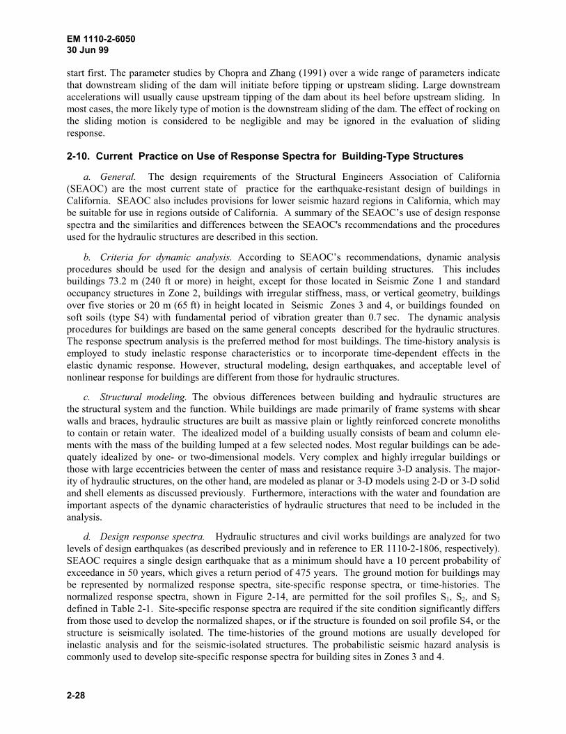
EM 1110-2-605030 Jun 99

2-28

start first. The parameter studies by Chopra and Zhang (1991) over a wide range of parameters indicatethat downstream sliding of the dam will initiate before tipping or upstream sliding. Large downstreamaccelerations will usually cause upstream tipping of the dam about its heel before upstream sliding. Inmost cases, the more likely type of motion is the downstream sliding of the dam. The effect of rocking onthe sliding motion is considered to be negligible and may be ignored in the evaluation of slidingresponse.

2-10. Current Practice on Use of Response Spectra for Building-Type Structures

a. General. The design requirements of the Structural Engineers Association of California(SEAOC) are the most current state of practice for the earthquake-resistant design of buildings inCalifornia. SEAOC also includes provisions for lower seismic hazard regions in California, which maybe suitable for use in regions outside of California. A summary of the SEAOC’s use of design responsespectra and the similarities and differences between the SEAOC's recommendations and the proceduresused for the hydraulic structures are described in this section.

b. Criteria for dynamic analysis. According to SEAOC’s recommendations, dynamic analysisprocedures should be used for the design and analysis of certain building structures. This includesbuildings 73.2 m (240 ft or more) in height, except for those located in Seismic Zone 1 and standardoccupancy structures in Zone 2, buildings with irregular stiffness, mass, or vertical geometry, buildingsover five stories or 20 m (65 ft) in height located in Seismic Zones 3 and 4, or buildings founded onsoft soils (type S4) with fundamental period of vibration greater than 0.7 sec. The dynamic analysisprocedures for buildings are based on the same general concepts described for the hydraulic structures.The response spectrum analysis is the preferred method for most buildings. The time-history analysis isemployed to study inelastic response characteristics or to incorporate time-dependent effects in theelastic dynamic response. However, structural modeling, design earthquakes, and acceptable level ofnonlinear response for buildings are different from those for hydraulic structures.

c. Structural modeling. The obvious differences between building and hydraulic structures arethe structural system and the function. While buildings are made primarily of frame systems with shearwalls and braces, hydraulic structures are built as massive plain or lightly reinforced concrete monolithsto contain or retain water. The idealized model of a building usually consists of beam and column ele-ments with the mass of the building lumped at a few selected nodes. Most regular buildings can be ade-quately idealized by one- or two-dimensional models. Very complex and highly irregular buildings orthose with large eccentricies between the center of mass and resistance require 3-D analysis. The major-ity of hydraulic structures, on the other hand, are modeled as planar or 3-D models using 2-D or 3-D solidand shell elements as discussed previously. Furthermore, interactions with the water and foundation areimportant aspects of the dynamic characteristics of hydraulic structures that need to be included in theanalysis.

d. Design response spectra. Hydraulic structures and civil works buildings are analyzed for twolevels of design earthquakes (as described previously and in reference to ER 1110-2-1806, respectively).SEAOC requires a single design earthquake that as a minimum should have a 10 percent probability ofexceedance in 50 years, which gives a return period of 475 years. The ground motion for buildings maybe represented by normalized response spectra, site-specific response spectra, or time-histories. Thenormalized response spectra, shown in Figure 2-14, are permitted for the soil profiles S1, S2, and S3

defined in Table 2-1. Site-specific response spectra are required if the site condition significantly differsfrom those used to develop the normalized shapes, or if the structure is founded on soil profile S4, or thestructure is seismically isolated. The time-histories of the ground motions are usually developed forinelastic analysis and for the seismic-isolated structures. The probabilistic seismic hazard analysis iscommonly used to develop site-specific response spectra for building sites in Zones 3 and 4.

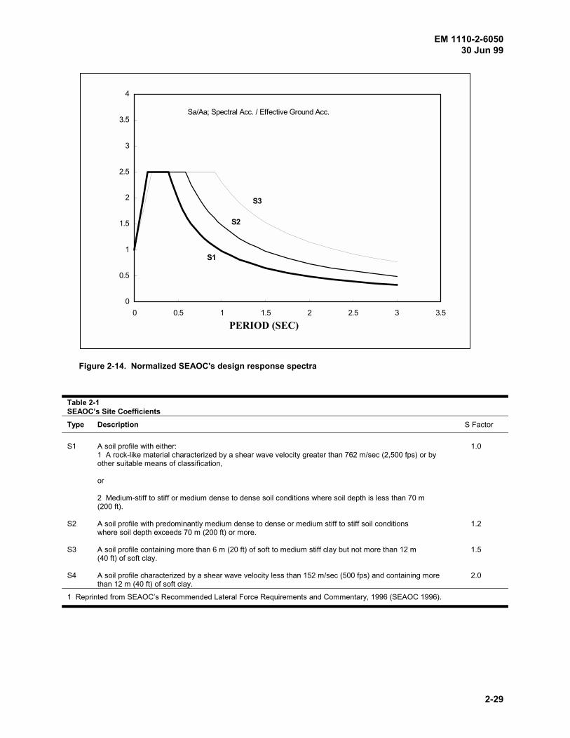
EM 1110-2-605030 Jun 99

2-29

Figure 2-14. Normalized SEAOC's design response spectra

Table 2-1SEAOC’s Site Coefficients

Type Description S Factor

S1 A soil profile with either:1 A rock-like material characterized by a shear wave velocity greater than 762 m/sec (2,500 fps) or byother suitable means of classification,

or

2 Medium-stiff to stiff or medium dense to dense soil conditions where soil depth is less than 70 m(200 ft).

1.0

S2 A soil profile with predominantly medium dense to dense or medium stiff to stiff soil conditionswhere soil depth exceeds 70 m (200 ft) or more.

1.2

S3 A soil profile containing more than 6 m (20 ft) of soft to medium stiff clay but not more than 12 m(40 ft) of soft clay.

1.5

S4 A soil profile characterized by a shear wave velocity less than 152 m/sec (500 fps) and containing morethan 12 m (40 ft) of soft clay.

2.0

1 Reprinted from SEAOC’s Recommended Lateral Force Requirements and Commentary, 1996 (SEAOC 1996).

PERIOD (SEC)

0

0.5

1

1.5

2

2.5

3

3.5

4

0 0.5 1 1.5 2 2.5 3 3.5

S1

S2

S3

Sa/Aa; Spectral Acc. / Effective Ground Acc.

EM 1110-2-605030 Jun 99

2-30

" #W

wR

/gaSWsCV ($$

e. Nonlinear response of buildings. The design practice for buildings permits the structure torespond inelastically during a major earthquake but suffer only acceptable and predictable amounts ofdamage without collapse. The energy dissipated through such inelastic deformations is utilized to reducethe level of seismic design forces. According to the SEAOC's Commentary, structures designed inconformance with its recommendations should, in general, be able to

(1) Resist a minor level of earthquake ground motion without damage.

(2) Resist a moderate level of earthquake ground motion without structural damage, but possiblyexperience some nonstructural damage.

(3) Resist a major level of earthquake ground motion having an intensity equal to the strongesteither experienced or forecast at the building site, without collapse, but possibly with some structural aswell as nonstructural damage. To achieve such performance goals, SEAOC recommends that the designforces be determined by reducing the elastic forces obtained from linear analysis by the system qualityfactor Rw. The structural system quality factor Rw represents the overall ductility and energy dissipationcapacity of the system when strained beyond its elastic limit. The Rw values are selected according to theability of a particular system to sustain cyclic inelastic deformations without collapse. Factorscontributing to the actual selection of Rw include redundancy, reliability of as-built performance,inelastic load-deformation behavior, and changed damping and period modification with deformation.Experience indicates that buildings designed based on this procedure have exhibited adequateperformance in most cases. In addition to the ductility requirement, most seismic codes require alimitation on the story drift to limit nonstructural damage during more frequent earthquakes and to ensurebuilding stability under the major earthquakes. For tall buildings, the drift limitations may dictate anelastic design, even for MCE ground motions.

f. Inelastic design response spectra. For regular buildings, the code specified design seismic forcescan be estimated from

(2-29)

where

V = base shear

Cs = design seismic coefficient

W = weight of building

Sa = linear elastic response spectral acceleration

Rw = the structural system quality factor intended to account for ductility and energy dissipation when the structure deforms beyond the yield point

The design seismic coefficient Cs can be obtained from a reduced response spectrum that can beconsidered to be the inelastic design response spectrum (IDRS). However, recent statistical studieshave shown that the shape of IDRS significantly differs from the shape of elastic response spectra(Miranda 1992; Krawinkler and Rahnama 1992), and is strongly influenced by the level of inelastic

EM 1110-2-605030 Jun 99

2-31

deformation, local site conditions, and the period of vibration. Until more data become available, themost reliable procedure for establishing an IDRS is to perform nonlinear dynamic time-history analysesof structures with different degrees of ductility ratios using the available recorded ground motions.

g. Nonlinear inelastic response of reinforced concrete hydraulic structures.

(1) Free-standing intake towers. The response of a free-standing intake tower to earthquake groundshaking is similar to that of a cantilever wall that resists earthquake forces by flexural and sheardeformations. Thus, the principles of inelastic design of reinforced concrete walls are generallyapplicable to free-standing towers, provided that the response is consistent with the post-yield capacity ofreinforced tower structure. Similar to the structural walls with limited ductility, intake towers should bedesigned such that flexural yielding controls the strength, the inelastic deformations, and thus the energydissipation in the entire structure (Pauly 1986). Failure modes due to diagonal tension or diagonalcompression caused by shear and sliding shear along the base of the structure should be avoided. Themain source of energy dissipation should be yielding of flexural reinforcement in the region where theplastic hinges are expected to develop. Recent research at CEWES has demonstrated that a lightlyreinforced rectangular intake tower possesses sufficient ductility to allow formation of a plastic hinge atthe base of the tower with a limited amount of inelastic behavior. The ability of such plastic hinges tosustain the repeated cycles of inelastic demands imposed on them, the expected length of the plastichinge, and the acceptable level of damage during major earthquakes are being investigated at CEWES.Until these have been established, preliminary design and screening evaluations for retangular intaketowers should be limited to an inelastic response not greater than twice the yield deflection in accordancewith the design provisions of EM 1110-2-2400.

(2) Other reinforced concrete hydraulic structures. For other reinforced concrete hydraulic structureswith structural configurations and systems different from those of buildings and intake towers, postelasticanalyses should be performed to establish appropriate ductility for the members so that the structure willundergo controlled levels of nonlinearity without compromising structural safety. Designing for to MDEtake advantage of the ability of the structures to dissipate energy through inelastic deformations shouldproduce uniform patterns of yielding and energy absorption. While the initial forces are distributedthrough the structure according to the elastic stiffness of the various members and connections, partiallydeveloped plastic hinges in the critical members will redistribute forces to the stiffer members and maynot follow the load paths envisioned in the initial design. If the desired level of ductility is not reached orthe forces are not distributed appropriately, then it is possible that the actual member forces may exceedthe design values. In addition, the possibility that all cycles of nonlinear response (i.e., hysteretic energydemand), and not just the maximum response cycle, may cause damage should also be investigated. Inother words, it is important to note that the specified ductility may be reached either once or severaltimes during the ground shaking, and to ensure that the lightly reinforced concrete hydraulic structure hassufficient ductility to resist such repeated demands. These considerations indicate that the inelasticdesign of hydraulic structures requires careful attention to the actual postelastic behavior of the structureand should be done in consultation with and approved by CECW-ET.

EM 1110-2-605030 Jun 99

3-1

Chapter 3Development of Site-Specific Response Spectra for SeismicAnalysis of Concrete Hydraulic Structures

Section IIntroduction

3-1. Purpose and Scope

This chapter describes procedures for developing site-specific response spectra of ground motionsthroughout the United States for seismic analyses of hydraulic structures. Also covered, but in less detail,are approaches for developing acceleration time-histories of ground motions. Section I provides an over-view of the general approaches to developing site-specific response spectra, a brief discussion of factorsinfluencing earthquake ground motions, and a brief discussion of differences in ground motion charac-teristics in different regions of the United States. This is followed in Sections II and III by descriptionsof procedures for developing site-specific response spectra using deterministic and probabilisticapproaches, respectively.

3-2. General Approaches for Developing Site-Specific Response Spectra

The two general approaches for developing site-specific response spectra are the deterministic andprobabilistic approaches.

a. Deterministic approach.

(1) General. In this approach, often termed a deterministic seismic hazard analysis, or DSHA, siteground motions are deterministically estimated for a specific, selected earthquake, that is, an earthquakeof a certain size on a specific seismic source occurring at a certain distance from the site. The earthquakesize may be characterized by magnitude or by epicentral intensity. In the WUS, the practice has been touse magnitude, whereas in the EUS, both magnitude and Modified Mercalli Intensity (MMI) have beenused. However, in the EUS, magnitude is increasingly being used as the measure of earthquake size, andground motions are correspondingly being estimated using correlations with magnitude. In this manual,ground motions are estimated using relationships with magnitude. For procedures for estimating groundmotions as a function of intensity, reference should be made to the state-of-the-art publication byKrinitzsky and Chang (1987).

(2) Size and location of design earthquakes. In the deterministic approach, earthquake magnitude istypically selected to be the magnitude of the largest earthquake judged to be capable of occurring on theseismic source, i.e., MCE. The selected earthquake is usually assumed to occur on the portion of theseismic source that is closest to the site (an exception is the “random earthquake” analysis described inSection II and Appendix D). After the earthquake magnitude and distance are selected, the site groundmotions are then estimated using ground motion attenuation relationships or other techniques.Procedures for deterministically estimating earthquake ground motions are described in Section II.

b. Probabilistic approach. In the probabilistic approach, often termed a probabilistic seismichazard analysis, or PSHA, site ground motions are estimated for selected values of the probability ofground motion exceedance in a design time period or for selected values of annual frequency or returnperiod for ground motion exceedance. As an example, ground motions could be estimated for a 10

EM 1110-2-605030 Jun 99

3-2

percent probability of exceedance in 100 years or for a return period of 950 years. The probabilisticapproach thus provides an expression of potential earthquake loading in terms analogous to those usedfor other environmental loads in civil engineering design such as wind and flood loading. A probabilisticground motion assessment incorporates the frequency of occurrence of earthquakes of differentmagnitudes on the seismic sources, the uncertainty of the earthquake locations on the sources, and theground motion attenuation including its uncertainty. Section III describes the procedures forprobabilistically estimating earthquake ground motions.

3-3. Factors Affecting Earthquake Ground Motions

a. General. As stated in paragraph 1-8, It has been well-recognized that earthquake ground motionsare affected by earthquake source conditions, source- to-site transmission path properties, and site condi-tions. The source conditions include the stress drop, source depth, size of the rupture area, slipdistribution (amount and distribution of static displacement on the fault plane), rise time (time for thefault slip to complete at a given point on the fault plane), type of faulting, and rupture directivity. Thetransmission path properties include the crustal structure and the shear-wave velocity and dampingcharacteristics of the crustal rock. The site conditions include the rock properties beneath the site todepths of up to about 2 km, the local soil conditions at the site to depths of up to several hundred feet,and the topography of the site. In developing relationships for estimating ground motions, the effects ofsource, path, and site have been commonly represented in a simplified manner by earthquake magnitude,source-to-site distance, and local subsurface conditions. The important influences of these factors onground motion are summarized below.

b. Effects of earthquake magnitude and distance on ground motions.

(1) General. The effects of earthquake magnitude and distance on the amplitude of ground motionsare well known; ground motion amplitudes tend to increase with increasing magnitude and decreasingdistance. However, the effects of magnitude and source-to-site distance on relative frequency content(response spectral shape) and duration of ground motions are not as well known and therefore are brieflyreviewed below.

(2) Effects of magnitude. The Guerrero, Mexico, accelerograph array data illustrate the large effectof magnitude on the relative frequency content and duration of earthquake ground motions. TheGuerrero array has provided recordings of rock motions over a wide range of magnitudes. Figures 3-1and 3-2 show the accelerograms and the corresponding response spectra for six recordings selected byAnderson and Quaas (1988) to be approximately equally spaced in magnitude from the smallest event ofmagnitude 3.1 to the largest of magnitude 8.1. Figure 3-1 illustrates the effect of magnitude on theduration of the strong shaking part of an accelerogram; with increasing magnitude, duration rapidlyincreases. All events have epicenters about 25 km from the station, and all stations are on hard rock(Anderson and Quaas 1988). Figure 3-2 illustrates that the larger magnitude events have somewhatlarger spectral amplitudes at high frequencies and much larger spectral amplitudes at long periods. Inother words, increasing magnitude results in greatly enriched relative frequency content (higher spectralshapes) at long periods. Figure 3-3 illustrates a generalization of the effect of magnitude on responsespectral shape, in this case, from the empirically based attenuation relationships for rock developed bySadigh et al. (1993).

(3) Effects of distance. Data from the Loma Prieta earthquake of October 17, 1989, provide anexample of the effect of distance on response spectral shape. Figure 3-4 shows that the spectral shape ofthe recordings obtained on rock during this earthquake reduce in the high-frequency range and increasein the long-period range with increasing distance. A generalization of the effect of distance on spectral

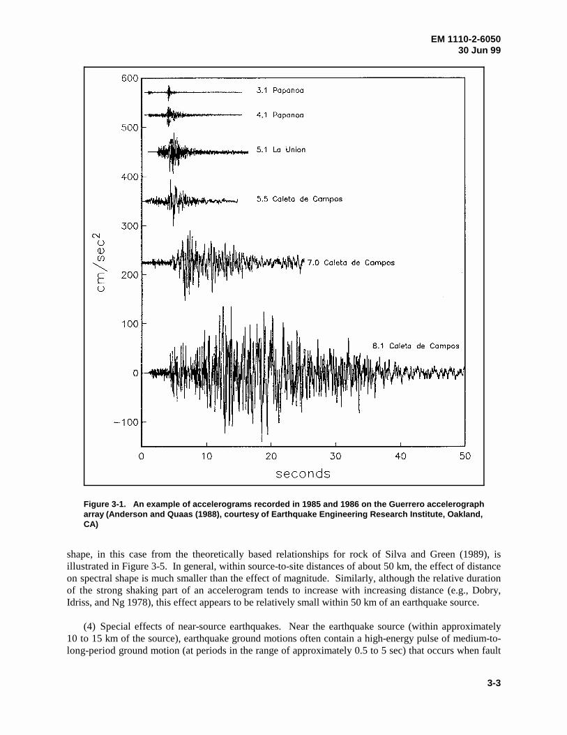
EM 1110-2-605030 Jun 99

3-3

Figure 3-1. An example of accelerograms recorded in 1985 and 1986 on the Guerrero accelerographarray (Anderson and Quaas (1988), courtesy of Earthquake Engineering Research Institute, Oakland,CA)

shape, in this case from the theoretically based relationships for rock of Silva and Green (1989), isillustrated in Figure 3-5. In general, within source-to-site distances of about 50 km, the effect of distanceon spectral shape is much smaller than the effect of magnitude. Similarly, although the relative durationof the strong shaking part of an accelerogram tends to increase with increasing distance (e.g., Dobry,Idriss, and Ng 1978), this effect appears to be relatively small within 50 km of an earthquake source.

(4) Special effects of near-source earthquakes. Near the earthquake source (within approximately10 to 15 km of the source), earthquake ground motions often contain a high-energy pulse of medium-to-long-period ground motion (at periods in the range of approximately 0.5 to 5 sec) that occurs when fault

EM 1110-2-605030 Jun 99

3-4

Figure 3-2. Response spectra (5 percent damped, pseudo-relative velocity)corresponding to the acceleration traces in Figure 3-1 (Anderson and Quaas (1988),courtesy of Earthquake Engineering Research Institute, Oakland, CA)

rupture propagates toward a site. It has also been found that these pulses exhibit a strong directionality,with the component of motion perpendicular (normal) to the strike of the fault being larger than thecomponent parallel to the strike (see, for example, Sadigh et al. 1993; Somerville and Graves 1993;Somerville et al. 1997). These characteristics of near-source ground motions are illustrated by theRinaldi recording obtained during the 1994 Northridge earthquake (Figure 3-6). These characteristicsshould be included in ground motion characterization for near-source earthquakes.

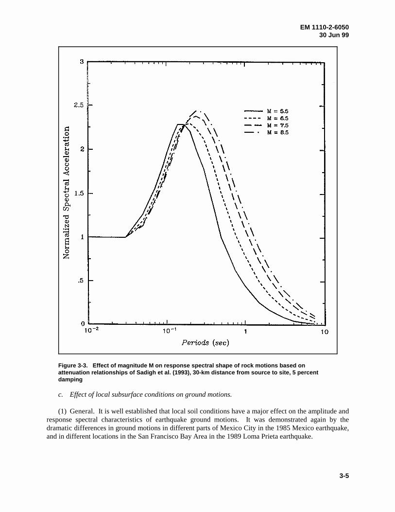
EM 1110-2-605030 Jun 99

3-5

Figure 3-3. Effect of magnitude M on response spectral shape of rock motions based onattenuation relationships of Sadigh et al. (1993), 30-km distance from source to site, 5 percentdamping

c. Effect of local subsurface conditions on ground motions.

(1) General. It is well established that local soil conditions have a major effect on the amplitude andresponse spectral characteristics of earthquake ground motions. It was demonstrated again by thedramatic differences in ground motions in different parts of Mexico City in the 1985 Mexico earthquake,and in different locations in the San Francisco Bay Area in the 1989 Loma Prieta earthquake.

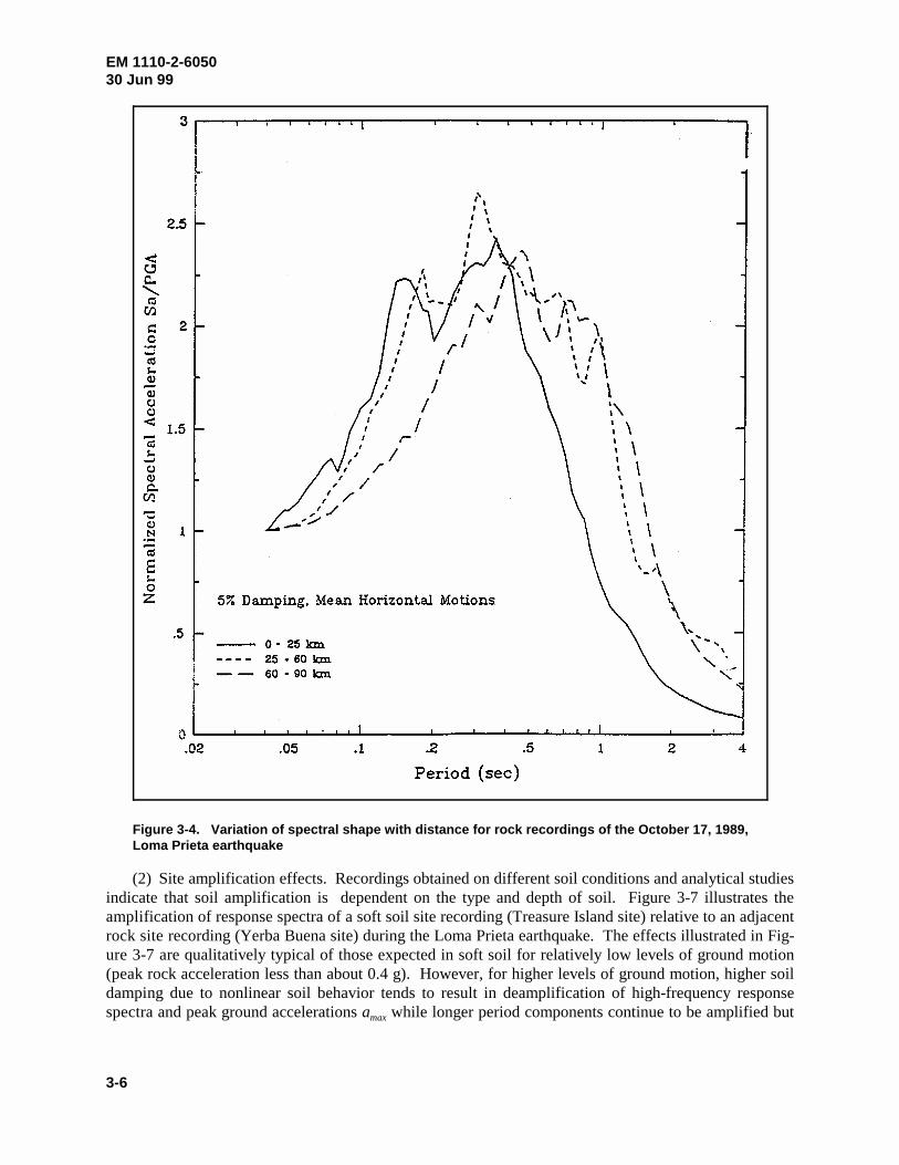
EM 1110-2-605030 Jun 99

3-6

Figure 3-4. Variation of spectral shape with distance for rock recordings of the October 17, 1989,Loma Prieta earthquake

(2) Site amplification effects. Recordings obtained on different soil conditions and analytical studiesindicate that soil amplification is dependent on the type and depth of soil. Figure 3-7 illustrates theamplification of response spectra of a soft soil site recording (Treasure Island site) relative to an adjacentrock site recording (Yerba Buena site) during the Loma Prieta earthquake. The effects illustrated in Fig-ure 3-7 are qualitatively typical of those expected in soft soil for relatively low levels of ground motion(peak rock acceleration less than about 0.4 g). However, for higher levels of ground motion, higher soildamping due to nonlinear soil behavior tends to result in deamplification of high-frequency responsespectra and peak ground accelerations a while longer period components continue to be amplified butmax

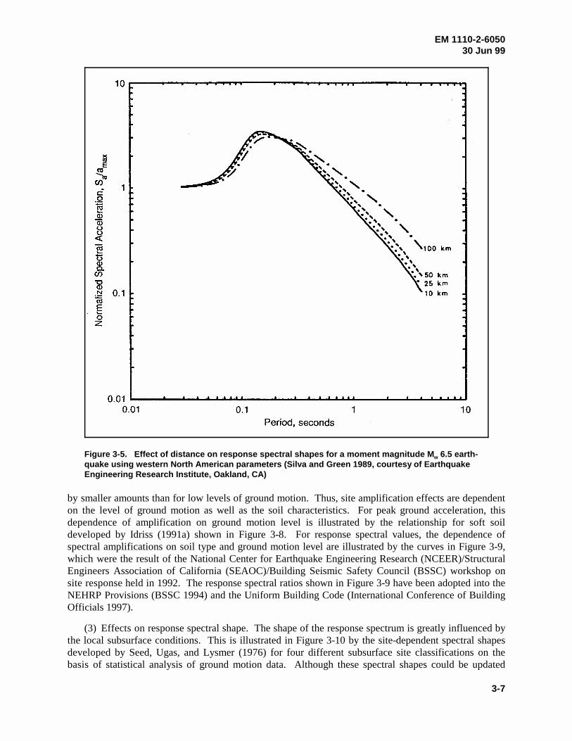
EM 1110-2-605030 Jun 99

3-7

Figure 3-5. Effect of distance on response spectral shapes for a moment magnitude M 6.5 earth-w

quake using western North American parameters (Silva and Green 1989, courtesy of EarthquakeEngineering Research Institute, Oakland, CA)

by smaller amounts than for low levels of ground motion. Thus, site amplification effects are dependenton the level of ground motion as well as the soil characteristics. For peak ground acceleration, thisdependence of amplification on ground motion level is illustrated by the relationship for soft soildeveloped by Idriss (1991a) shown in Figure 3-8. For response spectral values, the dependence ofspectral amplifications on soil type and ground motion level are illustrated by the curves in Figure 3-9,which were the result of the National Center for Earthquake Engineering Research (NCEER)/StructuralEngineers Association of California (SEAOC)/Building Seismic Safety Council (BSSC) workshop onsite response held in 1992. The response spectral ratios shown in Figure 3-9 have been adopted into theNEHRP Provisions (BSSC 1994) and the Uniform Building Code (International Conference of BuildingOfficials 1997).

(3) Effects on response spectral shape. The shape of the response spectrum is greatly influenced bythe local subsurface conditions. This is illustrated in Figure 3-10 by the site-dependent spectral shapesdeveloped by Seed, Ugas, and Lysmer (1976) for four different subsurface site classifications on thebasis of statistical analysis of ground motion data. Although these spectral shapes could be updated

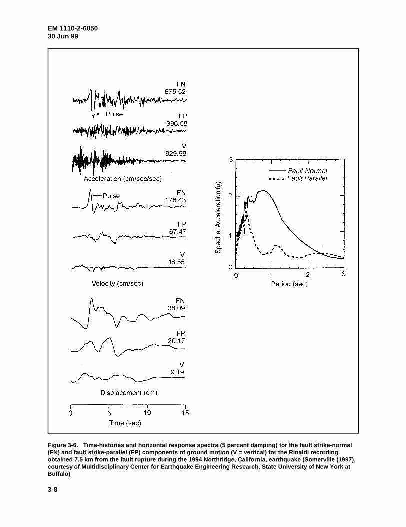
EM 1110-2-605030 Jun 99

3-8

Figure 3-6. Time-histories and horizontal response spectra (5 percent damping) for the fault strike-normal(FN) and fault strike-parallel (FP) components of ground motion (V = vertical) for the Rinaldi recordingobtained 7.5 km from the fault rupture during the 1994 Northridge, California, earthquake (Somerville (1997),courtesy of Multidisciplinary Center for Earthquake Engineering Research, State University of New York atBuffalo)

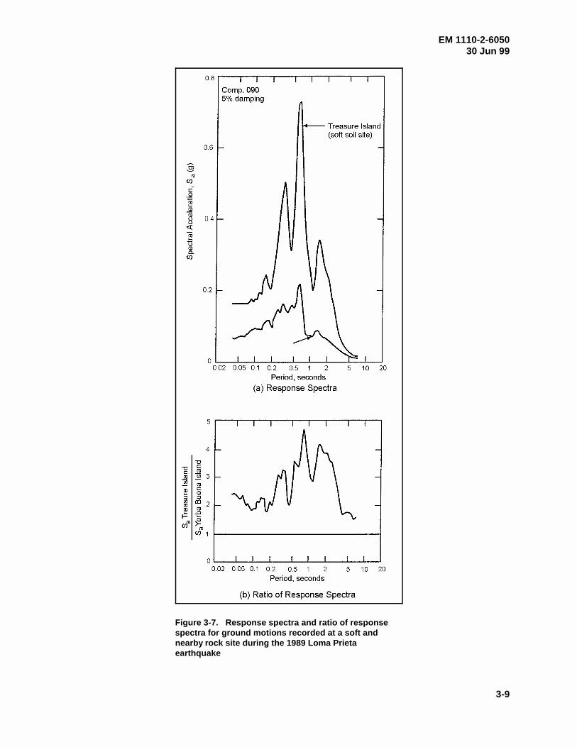
EM 1110-2-605030 Jun 99

3-9

Figure 3-7. Response spectra and ratio of responsespectra for ground motions recorded at a soft andnearby rock site during the 1989 Loma Prietaearthquake

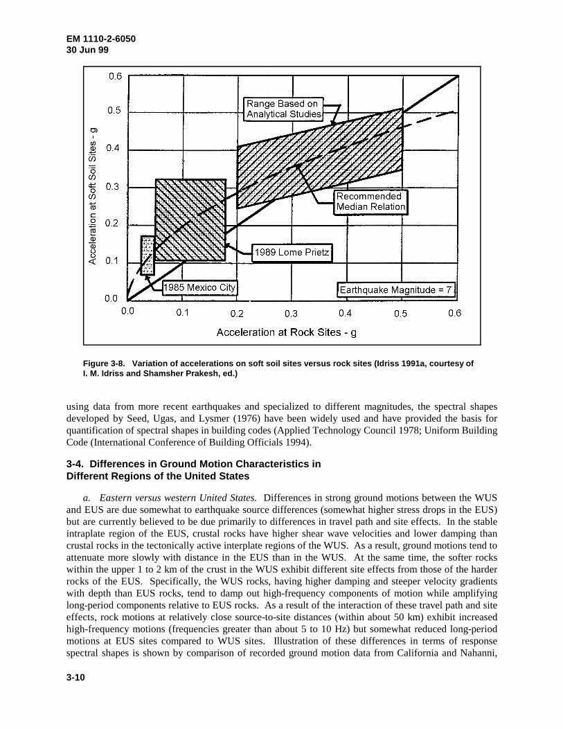
EM 1110-2-605030 Jun 99

3-10

Figure 3-8. Variation of accelerations on soft soil sites versus rock sites (Idriss 1991a, courtesy ofI. M. Idriss and Shamsher Prakesh, ed.)

using data from more recent earthquakes and specialized to different magnitudes, the spectral shapesdeveloped by Seed, Ugas, and Lysmer (1976) have been widely used and have provided the basis forquantification of spectral shapes in building codes (Applied Technology Council 1978; Uniform BuildingCode (International Conference of Building Officials 1994).

3-4. Differences in Ground Motion Characteristics inDifferent Regions of the United States

a. Eastern versus western United States. Differences in strong ground motions between the WUSand EUS are due somewhat to earthquake source differences (somewhat higher stress drops in the EUS)but are currently believed to be due primarily to differences in travel path and site effects. In the stableintraplate region of the EUS, crustal rocks have higher shear wave velocities and lower damping thancrustal rocks in the tectonically active interplate regions of the WUS. As a result, ground motions tend toattenuate more slowly with distance in the EUS than in the WUS. At the same time, the softer rockswithin the upper 1 to 2 km of the crust in the WUS exhibit different site effects from those of the harderrocks of the EUS. Specifically, the WUS rocks, having higher damping and steeper velocity gradientswith depth than EUS rocks, tend to damp out high-frequency components of motion while amplifyinglong-period components relative to EUS rocks. As a result of the interaction of these travel path and siteeffects, rock motions at relatively close source-to-site distances (within about 50 km) exhibit increasedhigh-frequency motions (frequencies greater than about 5 to 10 Hz) but somewhat reduced long-periodmotions at EUS sites compared to WUS sites. Illustration of these differences in terms of responsespectral shapes is shown by comparison of recorded ground motion data from California and Nahanni,

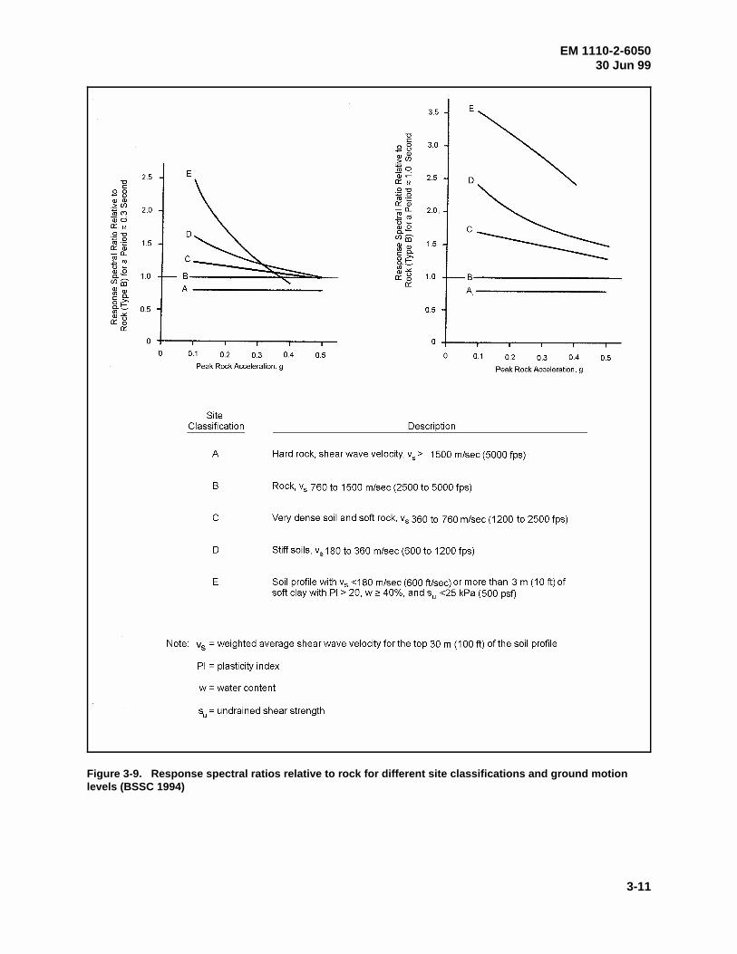
EM 1110-2-605030 Jun 99

3-11

Figure 3-9. Response spectral ratios relative to rock for different site classifications and ground motionlevels (BSSC 1994)

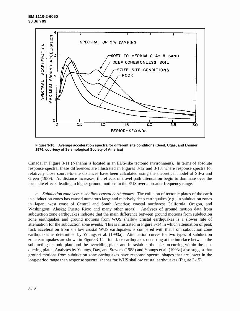
EM 1110-2-605030 Jun 99

3-12

Figure 3-10. Average acceleration spectra for different site conditions (Seed, Ugas, and Lysmer1976, courtesy of Seismological Society of America)

Canada, in Figure 3-11 (Nahanni is located in an EUS-like tectonic environment). In terms of absoluteresponse spectra, these differences are illustrated in Figures 3-12 and 3-13, where response spectra forrelatively close source-to-site distances have been calculated using the theoretical model of Silva andGreen (1989). As distance increases, the effects of travel path attenuation begin to dominate over thelocal site effects, leading to higher ground motions in the EUS over a broader frequency range.

b. Subduction zone versus shallow crustal earthquakes. The collision of tectonic plates of the earthin subduction zones has caused numerous large and relatively deep earthquakes (e.g., in subduction zonesin Japan; west coast of Central and South America; coastal northwest California, Oregon, andWashington; Alaska; Puerto Rico; and many other areas). Analyses of ground motion data fromsubduction zone earthquakes indicate that the main difference between ground motions from subductionzone earthquakes and ground motions from WUS shallow crustal earthquakes is a slower rate ofattenuation for the subduction zone events. This is illustrated in Figure 3-14 in which attenuation of peakrock acceleration from shallow crustal WUS earthquakes is compared with that from subduction zoneearthquakes as determined by Youngs et al. (1993a). Attenuation curves for two types of subductionzone earthquakes are shown in Figure 3-14—interface earthquakes occurring at the interface between thesubducting tectonic plate and the overriding plate, and intraslab earthquakes occurring within the sub-ducting plate. Analyses by Youngs, Day, and Stevens (1988) and Youngs et al. (1993a) also suggest thatground motions from subduction zone earthquakes have response spectral shapes that are lower in thelong-period range than response spectral shapes for WUS shallow crustal earthquakes (Figure 3-15).

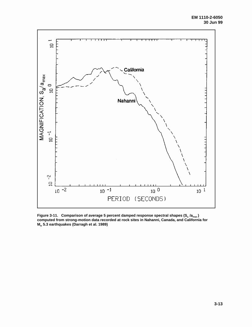
EM 1110-2-605030 Jun 99

3-13

Figure 3-11. Comparison of average 5 percent damped response spectral shapes (S /a )a max

computed from strong-motion data recorded at rock sites in Nahanni, Canada, and California forM 5.3 earthquakes (Darragh et al. 1989)w

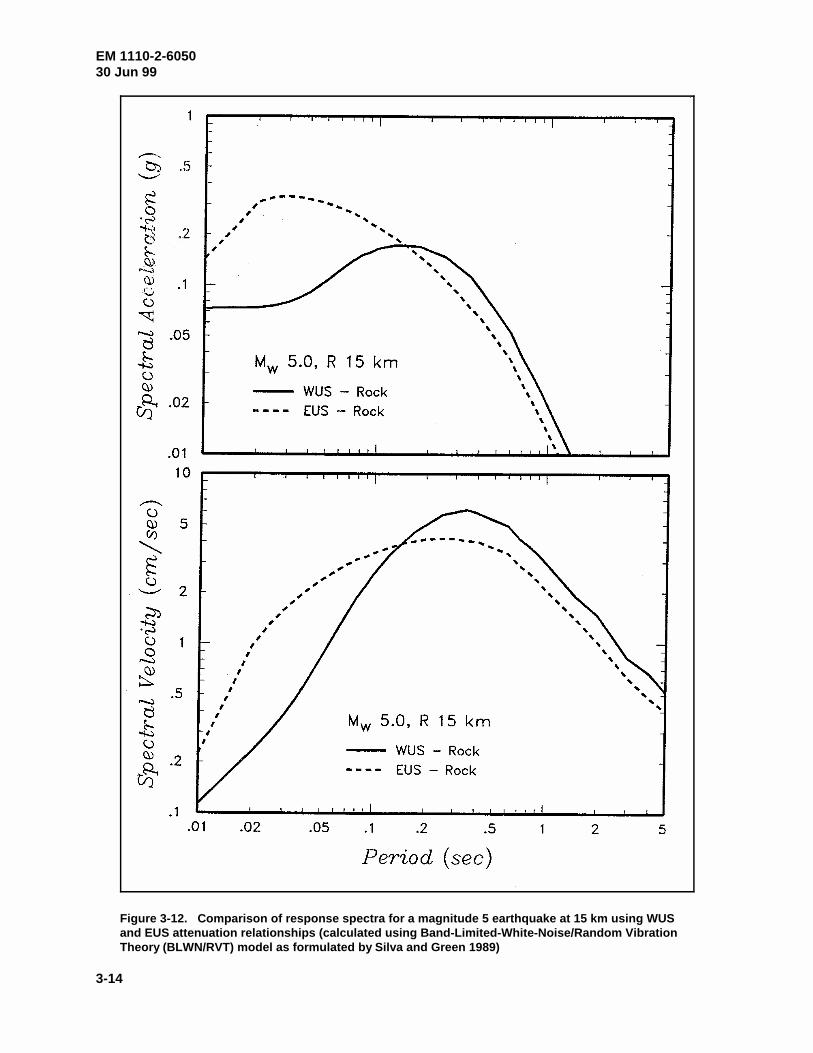
EM 1110-2-605030 Jun 99

3-14

Figure 3-12. Comparison of response spectra for a magnitude 5 earthquake at 15 km using WUSand EUS attenuation relationships (calculated using Band-Limited-White-Noise/Random VibrationTheory (BLWN/RVT) model as formulated by Silva and Green 1989)

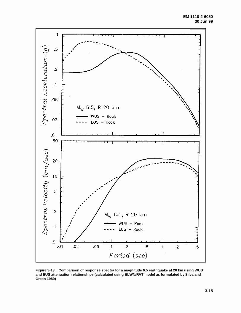
EM 1110-2-605030 Jun 99

3-15

Figure 3-13. Comparison of response spectra for a magnitude 6.5 earthquake at 20 km using WUSand EUS attenuation relationships (calculated using BLWN/RVT model as formulated by Silva andGreen 1989)

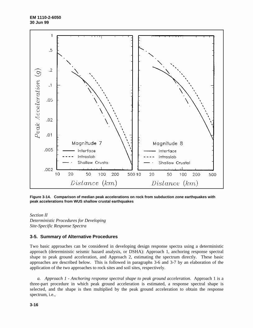
EM 1110-2-605030 Jun 99

3-16

Figure 3-14. Comparison of median peak accelerations on rock from subduction zone earthquakes withpeak accelerations from WUS shallow crustal earthquakes

Section IIDeterministic Procedures for DevelopingSite-Specific Response Spectra

3-5. Summary of Alternative Procedures

Two basic approaches can be considered in developing design response spectra using a deterministicapproach (deterministic seismic hazard analysis, or DSHA): Approach 1, anchoring response spectralshape to peak ground acceleration, and Approach 2, estimating the spectrum directly. These basicapproaches are described below. This is followed in paragraphs 3-6 and 3-7 by an elaboration of theapplication of the two approaches to rock sites and soil sites, respectively.

a. Approach 1 - Anchoring response spectral shape to peak ground acceleration. Approach 1 is athree-part procedure in which peak ground acceleration is estimated, a response spectral shape isselected, and the shape is then multiplied by the peak ground acceleration to obtain the responsespectrum, i.e.,

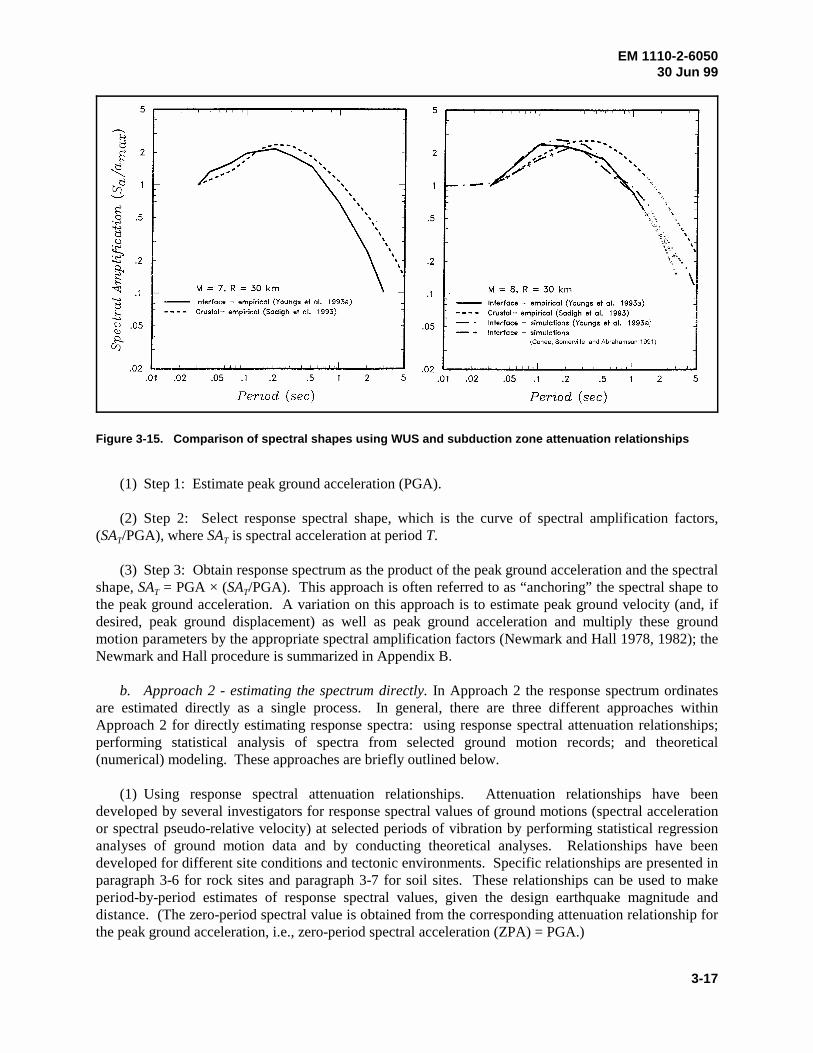
EM 1110-2-605030 Jun 99

3-17

Figure 3-15. Comparison of spectral shapes using WUS and subduction zone attenuation relationships

(1) Step 1: Estimate peak ground acceleration (PGA).

(2) Step 2: Select response spectral shape, which is the curve of spectral amplification factors,(SA /PGA), where SA is spectral acceleration at period T.T T

(3) Step 3: Obtain response spectrum as the product of the peak ground acceleration and the spectralshape, SA = PGA × (SA /PGA). This approach is often referred to as “anchoring” the spectral shape toT T

the peak ground acceleration. A variation on this approach is to estimate peak ground velocity (and, ifdesired, peak ground displacement) as well as peak ground acceleration and multiply these groundmotion parameters by the appropriate spectral amplification factors (Newmark and Hall 1978, 1982); theNewmark and Hall procedure is summarized in Appendix B.

b. Approach 2 - estimating the spectrum directly. In Approach 2 the response spectrum ordinatesare estimated directly as a single process. In general, there are three different approaches withinApproach 2 for directly estimating response spectra: using response spectral attenuation relationships;performing statistical analysis of spectra from selected ground motion records; and theoretical(numerical) modeling. These approaches are briefly outlined below.

(1) Using response spectral attenuation relationships. Attenuation relationships have beendeveloped by several investigators for response spectral values of ground motions (spectral accelerationor spectral pseudo-relative velocity) at selected periods of vibration by performing statistical regressionanalyses of ground motion data and by conducting theoretical analyses. Relationships have beendeveloped for different site conditions and tectonic environments. Specific relationships are presented inparagraph 3-6 for rock sites and paragraph 3-7 for soil sites. These relationships can be used to makeperiod-by-period estimates of response spectral values, given the design earthquake magnitude anddistance. (The zero-period spectral value is obtained from the corresponding attenuation relationship forthe peak ground acceleration, i.e., zero-period spectral acceleration (ZPA) = PGA.)

EM 1110-2-605030 Jun 99

3-18

Typically, these relationships have been developed for 5 percent damping; and ratios between spectralvalues at different damping ratios (e.g., Newmark and Hall 1978, 1982; Appendix B) are used to obtainthe corresponding spectra for other damping ratios.

(2) Performing statistical analysis of ground motion data. Spectral attenuation relationships dis-cussed above are based on all the available applicable ground motion data, and they typically cover awide range of earthquake magnitudes and distances. However, for a specific magnitude and distance, itmay be possible to obtain an improved or a comparative estimate of the response spectrum byperforming statistical analysis using a set of response spectra of ground motion records from earthquakeshaving magnitudes and distances that are close to the design magnitude and distance. The data set istypically a subset of the data used to develop attenuation relationships. The analysis may consist ofdirect, period-by-period statistical analysis of the data. However, it is also possible to “scale” or adjusteach response spectral value of each record to values for the design magnitude and distance and then dostatistical analysis of the scaled data set. The attenuation relationships for response spectral values(discussed in (1) above) are used to perform the scaling. This approach of scaling before performingstatistical analyses is recommended unless the magnitudes and distances for the data set are closelybunched around the design magnitude and distance. Appendix C illustrates the approach of statisticalanalyses of a set of scaled response spectra. A particular type of statistical analysis that has been usedfor many nuclear power plant sites in the EUS and for other sites and locations as well is termed a“random earthquake” analysis. This analysis is performed to estimate the response spectrum at a site dueto a randomly located (“floating”) earthquake within the vicinity of the site, i.e., when its location cannotbe assigned to a specific geologic structure at a specific distance from the site. After the designmagnitude of the random earthquake is selected, a statistical analysis is made of response spectra ofground motion records from earthquakes having magnitudes close to the design magnitude, recorded onsite conditions similar to those for the actual site, and recorded within a selected source-to-site distance,typically 25 km. A random earthquake analysis can also be performed using attenuation relationships.Appendix D illustrates a random earthquake analysis.

(3) Performing theoretical (numerical) ground motion modeling. The state of the art for theoretical(numerical) modeling of ground motions is being vigorously advanced and is being increasingly used forsite-specific project applications. Various methods attempt to simulate the earthquake rupture, thepropagation of seismic waves from earthquake source to site, and/or the effect of local site conditions. Anumber of methods have been developed. These methods warrant consideration as a supplementarymeans for ground motion estimation. They can be particularly useful for extrapolating to conditions thatlie outside those represented by the database of strong motion recordings. The methods vary consider-ably in degree of complexity and sophistication. One relatively simple model that has been usedincreasingly to simulate earthquake rupture and source-to-site wave propagation is the Band LimitedWhite Noise/Random Vibration Theory (BLWN/RVT) Model (Atkinson 1984; Atkinson and Boore1995; Boore 1983, 1986; Boore and Atkinson 1987; Boore and Joyner 1991; Hanks and McGuire 1981;McGuire, Toro, and Silva 1988; Silva and Green 1989). This method has been applied particularly in theEUS because of the relative scarcity of ground motion data in the EUS, and attenuation relationships forthe EUS have been developed using this model. A particular form of theoretical analysis applicable tosoil sites is “site response analysis,” or “ground response analysis” in which the objective is to assess themodifying influence of the local soil conditions on rock motions estimated for the site and, in thismanner, estimate the motions at the ground surface of the soil site. Site response analyses are discussedin paragraph 3-7 in the context of their use in estimating response spectra for soil sites.

c. Relative advantages of Approach 1 and Approach 2. Approach 2, estimating the spectrumdirectly, should be used rather than Approach 1, anchoring spectral shape to peak ground acceleration,

EM 1110-2-605030 Jun 99

3-19

because, as was outlined in Section I, spectral shapes depend on more than just the site conditions (i.e.,on tectonic environment, earthquake magnitude, and other factors), yet the readily available and widelyused spectral shapes generally incorporate only the effect of the local site conditions. Currently availableprocedures, relationships, and data enable response spectra to be estimated as a single process inApproach 2. When spectra are estimated using Approach 2, it is often useful to make comparative esti-mates using Approach 1. In paragraph 3-6 procedures and relationships for Approaches 1 and 2 fordeveloping response spectra for rock sites are discussed. A similar presentation is made in paragraph 3-7for soil sites.

3-6. Developing Site-Specific Spectra for Rock Sites

a. Using Approach 1 - Anchoring rock response spectral shape to peak rock acceleration.

(1) Estimating peak rock acceleration. Recently developed attenuation relationships for estimatingpeak rock acceleration for shallow crustal earthquakes in the WUS, for the EUS, and for subductionzones are summarized in Table 3-1. The relationships for the WUS shallow crustal earthquakes arebetter constrained than those for the other tectonic environments because of the relative abundance ofstrong motion data for WUS shallow earthquakes. The peak acceleration attenuation relationships inTable 3-1 generally include the standard deviations of the estimates, from which 84th percentile valuesmay be obtained.

Table 3-1Summary of Recently Developed Attenuation Relationships for Peak Ground Acceleration

Tectonic Environment Relationship Site Condition

WUS shallow earthquakes Idriss (1991b) Rock1

Idriss (1991a) Soft soil1

Sadigh et al. (1993) Rock1,2

Abrahamson and Silva (1997) Rock and deep firm soil1,2

Campbell (1997) Alluvium, soft rock, hard rock1,2

Boore, Joyner, and Fumal (1997) Four site classifications based on 1

shear wave velocity

Sadigh et al. (1997) Rock and deep firm soil1

EUS Boore and Joyner (1991) Deep soil

Frankel et al. (1996) Hard rock

Atkinson and Boore (1997) Hard rock

Toro, Abrahamson, and Schneider (1997) Hard rock

Subduction zone Crouse (1991) Firm soil

Molas and Yamazaki (1995) Rock; hard soil; medium soil; soft soil

Youngs et al. (1997) Rock and deep soil

Subduction zone and shallow Fukushima and Tanaka (1990) Rock; hard soil; medium soil; soft soilearthquakes (no distinction)

Krinitzsky, Chang, and Nuttli (1987) Hard site and soft site

Includes a factor for type of faulting.1

Including vertical ground motions.2

EM 1110-2-605030 Jun 99

3-20

(2) Estimating response spectral shape and the response spectrum. Available spectral shapes forrock site conditions are summarized in Table 3-2. Multiplying spectral shape times peak groundacceleration results in the absolute response spectrum. Using the Newmark and Hall (1978, 1982)approach (Appendix B), peak ground acceleration is multiplied by the acceleration amplification factor,peak ground velocity by the velocity amplification factor, and peak ground displacement by thedisplacement amplification factor. Newmark and Hall’s recommended relationships between peakground acceleration, peak ground velocity, and peak ground displacement for rock site conditions may beused to estimate peak ground velocity and peak ground displacement, given peak ground acceleration; orpeak ground velocity and peak ground displacement may be independently estimated. Note that therelationships in Table 3-2 of Seed, Ugas, and Lysmer (1976), Mohraz (1976), Applied TechnologyCouncil (1978), and Newmark and Hall (1978, 1982), do not explicitly incorporate the important effectsof magnitude on spectral shape. The relationships of Mohraz (1976) and Newmark and Hall (1978,1982) can indirectly incorporate the effects of magnitude through its effect on peak ground velocity andpeak ground displacement if these parameters are estimated independently from peak ground acceleration(Appendix B).

Table 3-2Summary of Available Response Spectral Shapes of Ground Motions

Tectonic Environment Relationship Site Conditions

WUS shallow earthquakes Seed, Ugas, and Lysmer (1976) Rock; stiff soil; deep cohesionlesssoil; soft to medium clay and sand

Mohraz (1976) Rock; shallow alluvium; moderatelydeep alluvium; alluvium

Applied Technology Council (1978) Rock or shallow stiff soil; deep stiff1

soil; soft soil

Newmark and Hall (1978, 1982) Rock; firm soil

Sadigh et al. (1997) Rock and deep firm soil

WUS shallow earthquakes; EUS Silva and Green (1989) Rock

Subduction zones Youngs et al. (1997) Rock and deep soil

These spectral shapes are based primarily on Seed, Ugas, and Lysmer (1976). The Applied Technology Council (1978) spectral1

shapes are also the spectral shapes that appear in the 1994 Uniform Building Code (International Conference of Building CodeOfficials 1994) and the 1995 Recommended Lateral Force Requirements and Commentary (“Blue Book”) of the SeismologyCommittee of the Structural Engineers Association of California (SEAOC 1996).

(3) Uncertainty in response spectral prediction. Response spectra obtained using the median ormean peak ground acceleration attenuation relationships and the median or mean spectral shapes sum-marized above result in median (50th percentile) or mean ground motion estimates, given a design earth-quake magnitude and distance. Additional consideration must be given if a higher percentile groundmotion is to be predicted, for example the 84th percentile (median plus standard deviation) groundmotion. Spectra for the 84th percentile can be estimated by multiplying median or mean peak groundacceleration by 84th percentile spectral shapes. For example, Seed, Ugas and Lysmer (1976) present84th percentile shapes as well as mean shapes. However, this procedure results in a lesser degree ofconservatism in the very short period part of the spectrum because the anchor value of peak groundacceleration (equal to the zero-period spectral acceleration, ZPA) is at the median or mean level. Inorder to have a uniform degree of conservatism throughout the period range, the peak ground accelera-tion and the very short period part of the spectrum should be adjusted upward to the 84th percentile level.Alternatively, the entire median response spectrum may be scaled upward by a factor to the approximate84th percentile level. When the entire spectrum is scaled, often the standard deviation in peak groundacceleration is used to obtain a scaling factor. This is an approximation, since the standard deviation has

EM 1110-2-605030 Jun 99

3-21

been found to vary with period of vibration. (The period dependence can be directly accounted for whenusing Approach 2.) The 84th percentile amplification factors of the Newmark and Hall (1978, 1982)approach can be applied to median estimates of peak ground acceleration, velocity, and displacement toobtain 84th percentile spectral values (Appendix B, Table B-1). Again, a separate adjustment should beapplied to raise the peak ground acceleration and very short period part of the spectrum to the 84thpercentile level.

(4) Estimating vertical ground motion response spectra. Ratios of vertical to horizontal responsespectral amplitudes can be used to estimate vertical response spectra, given an estimate of horizontalresponse spectra. Recent studies (e.g., Silva 1997) indicate that vertical-to-horizontal response spectralratios are a function of period of vibration, earthquake source to site distance, earthquake magnitude,tectonic environment (WUS and EUS), and subsurface conditions (soil and rock). Figure 3-16 provides aguideline for ratios of vertical to horizontal spectral values on rock sites that is generally conservative forearthquake magnitudes equal to or less than about 6.5. However, if a facility is sensitive to short-period(less than 0.3 sec) vertical motions, and is located within 10 km of the earthquake source or the magni-tude exceeds 6.5, further evaluation of vertical response spectra on rock is recommended because verticalresponse spectra can significantly exceed horizontal response spectra for these conditions.

b. Using Approach 2 - Estimating the rock response spectrum directly.

(1) General. The three approaches discussed in paragraph 3-5b can be used: using response spectralattenuation relationships, performing statistical analyses of ground motion response spectra, andtheoretical (numerical) modeling. The following paragraphs refer to particular relationships or methods.

(2) Using response spectral attenuation relationships. Recently developed attenuation relationshipsthat can be used to predict horizontal rock response spectral values for WUS shallow crustal earthquakes,for EUS earthquakes, and for subduction zone earthquakes are summarized in Table 3-3. The spectralacceleration attenuation relationships summarized in Table 3-3 generally include the standard deviationsof the estimates, from which 84th percentile values may be obtained. As illustrated in Figures 3-12 and3-13, EUS attenuation models characteristically estimate much higher spectral response in the short-period range (less than 0.1 to 0.2 sec) than estimated by relationships for the WUS. As discussed inparagraph 3-4a the higher short-period response is attributed to the hardness of the rock in the EUS.Such short-period (high-frequency) motions may or may not be significant to the response andperformance of hydraulic structures. The assessment of the significance of such motions should be madeby the principal design engineer in collaboration with the seismic structural analyst and the materialsengineer.

(3) Using statistical analyses of response spectra. Abundant strong motion data are available to per-mit statistical analyses of data sets for many design earthquake scenarios for WUS shallow crustal earth-quakes. As noted in paragraph 3-5b(2), statistical “random earthquake” analyses have been made atmany EUS sites because, in general, discrete faults have not been identified in the EUS. Yet it wasdesired to model the possibility of an earthquake (usually of moderate magnitude, in the range of magni-tude 5 to 6) occurring near the site. Many of these analyses have been carried out using WUS groundmotion data because only a few records from moderate magnitude earthquakes are available in the EUS.Such analyses may be reasonable for estimating longer period rock motions but would apparently under-estimate shorter period (less than 0.1 to 0.3 sec) ground motions at hard rock sites. In this case, anadjustment should be made for the short-period response spectral values, if these short-period motionsare of significance to the structure under consideration. The adjustment can be made by comparing

EM 1110-2-605030 Jun 99

3-22

Figure 3-16. Simplified relationships between vertical and horizontal response spectra as a function ofdistance R

EM 1110-2-605030 Jun 99

3-23

Table 3-3Summary of Recently Developed Attenuation Relationships for Response Spectral Values of Ground Motions

Tectonic Environment Relationship Site Conditions

WUS shallow earthquakes Idriss (1991b) Rock1

Sadigh et al. (1993) Rock1,2

Abrahamson and Silva (1997) Rock and deep firm soil1,2

Campbell (1997) Alluvium, soft rock, hard rock1,2

Boore, Joyner, and Fumal (1997) Four site classifications based on1

shear wave velocity

Sadigh et al. (1997) Rock and deep firm soil1

EUS Boore and Joyner (1991) Deep soil

Frankel et al. (1996) Hard rock

Atkinson and Boore (1997) Hard rock

Toro, Abrahamson, and Schneider (1997) Hard rock

Subduction zone Crouse (1991) Firm soil

Youngs et al. (1997) Rock and deep soil

Includes a factor for type of faulting.1

Including vertical ground motions.2

response spectrum amplitudes predicted by EUS and WUS attenuation relationships for rock (Table 3-3).As illustrated in Appendix D, a random earthquake analysis can also be carried out using attenuationrelationships. Thus this analysis can be performed using the EUS spectral attenuation relationships thatpredict higher short-period motions at hard rock sites.

(4) Using theoretical (numerical) modeling techniques. The techniques discussed in para-graph 3-5b(3) can be used. These techniques attempt to simulate the earthquake rupture and the propaga-tion of seismic waves from the earthquake source to the site.

(5) Estimating vertical ground motion response spectra. The available recently developed attenua-tion relationships for response spectral values of vertical rock motions are summarized in Table 3-3.These relationships can be used directly to estimate vertical rock response spectra. The vertical to hori-zontal spectral ratios discussed in paragraph 3-6a(4) and shown in Figure 3-16 can be used as a guide inestimating vertical response spectra, given an estimate of the horizontal spectra.

c. Developing acceleration time-histories of rock motions consistent with the design responsespectrum.

(1) General. When acceleration time-histories of ground motions are required for the dynamicanalysis of a structure, they should be developed to be consistent with the design response spectrum overthe period range of significance for the structure, as well as have an appropriate strong motion durationfor the particular design earthquake. Two general approaches to developing acceleration time-historiesare selecting a suite of recorded motions and synthetically developing or modifying one or more motions.

EM 1110-2-605030 Jun 99

3-24

These approaches are discussed below. For either approach, when near-source earthquake groundmotions are modeled, it may be desirable that an acceleration time-history include a strong intermediate-to long-period pulse to model this particular characteristic of ground motion often observed in the nearfield (paragraph 3-3b(4) and Figure 3-6).

(2) Selecting recorded motions. Every earthquake produces a unique set of acceleration time-histories having characteristics that depend on the earthquake magnitude and other source characteristics,distance, attenuation and other travel path characteristics, and local site conditions. The response spec-trum of any individual ground motion accelerogram has peaks and valleys that occur at different periodsof vibration. Thus, the response spectrum of any single accelerogram is unlikely to match the developedsmooth design response spectrum. Typically, when recorded motions are selected, it is necessary tochoose a suite of time-histories (typically at least four) such that, in aggregate, valleys of individualspectra that fall below the design curve are covered by peaks of other spectra and (preferably) theexceedance of the design spectrum by individual spectral peaks is not excessive. For nonlinear analyses,it may be desirable to have additional time-histories because of the importance of pulse sequencing tononlinear response (see also comments in (3) below). In the approach of selecting recorded motions,simple scaling of individual accelerograms by a constant factor is done to improve the spectral fit, but thewave form and the relative spectral content of the accelerograms are not modified. The advantage ofselecting recorded motions is that each accelerogram is an actual recording, and thus the structure isanalyzed for natural motions that are presumably most representative of what the structure could expe-rience. The approach has the following disadvantages: multiple dynamic analyses are needed for thesuite of accelerograms selected; although a suite of accelerograms is selected, there will typically besubstantial exceedances of the smooth design spectrum by individual spectrum peaks; and although areasonably good spectral fit may be achieved for one horizontal component, when the same simplescaling factors are applied to the other horizontal components and the vertical components for the recordsselected, the spectral fit is usually not as good for the other components.

(3) Synthetically developing or modifying motions. A number of techniques and computer programshave been developed either to completely synthesize an accelerogram or modify a recorded accelerogramso that the response spectrum of the resultant accelerogram closely fits or matches the design spectrum.It is preferred to use techniques that modify a recorded accelerogram rather than completely synthesize amotion since the recorded motion will have time-domain characteristics representative of actual groundmotions. Two techniques that have been found to do a good job of spectrally modifying recordedmotions are the frequency-domain RASCAL computer code developed for the Corps of Engineers bySilva and Lee (1987) and the time-domain technique developed by Lilhanand and Tseng (1988). Thesetechniques preserve the basic time-domain character of the accelerogram yet provide an excellent matchto a smooth spectrum. An example of the spectral matching technique is given in Figures 3-17 and 3-18.The RASCAL computer code was used in this case. Figure 3-17 illustrates the initial (recorded)acceleration, velocity, and displacement time-histories and the time-histories after the spectral matchingprocess. Figure 3-18 illustrates the initial (recorded) acceleration response spectra, the smooth designresponse spectrum, and the response spectrum of the acceleration time-history after the spectral matchingprocess. Figure 3-18 illustrates the very close spectral match that was achieved, while Figure 3-17illustrates that the modified time-histories preserve the basic time-domain character of the originalrecord. Synthetic techniques for developing time-histories have the following advantages: a good fit tothe design spectrum can be achieved with a single accelerogram; the natural appearance and strongmotion duration can be maintained in the accelerograms; and three component motions (two horizontaland one vertical) each providing a good spectral match can be developed, and these can be madestatistically independent if desired; and the process is relatively efficient.

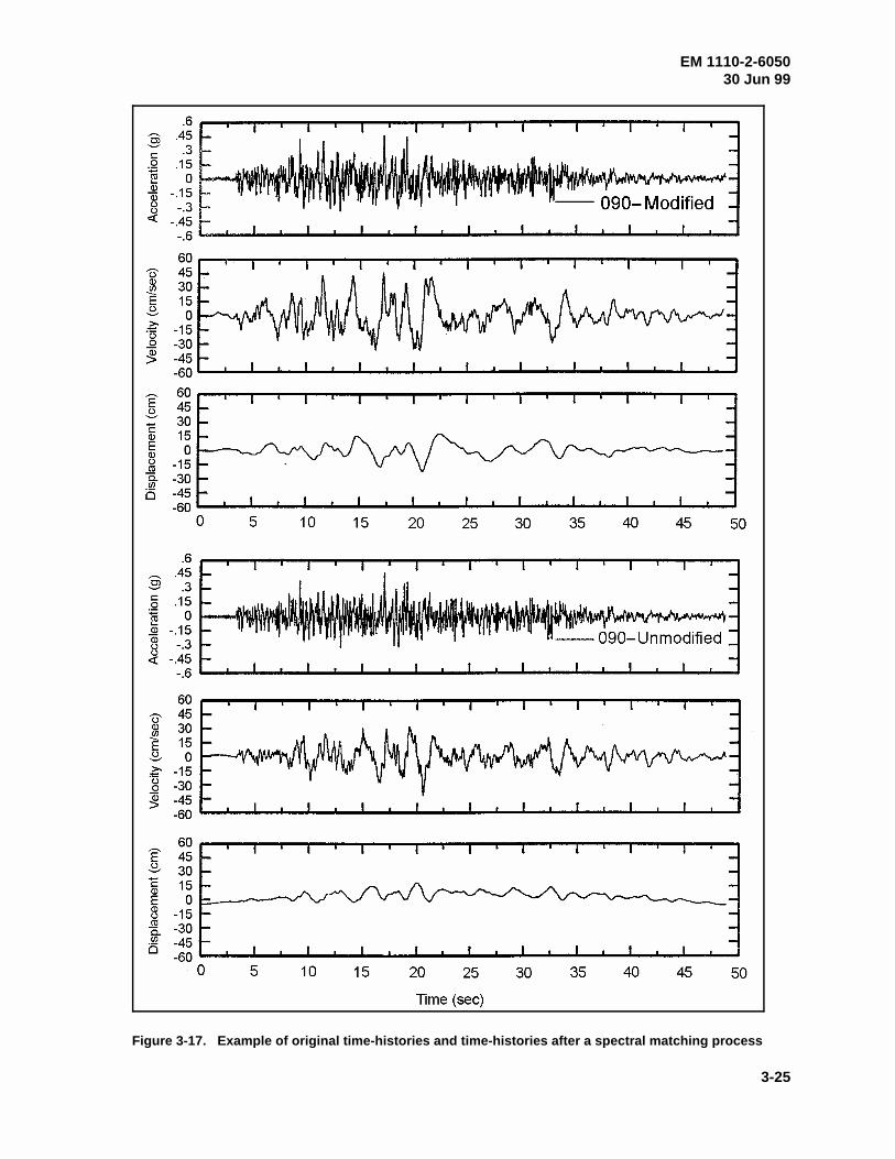
EM 1110-2-605030 Jun 99

3-25

Figure 3-17. Example of original time-histories and time-histories after a spectral matching process

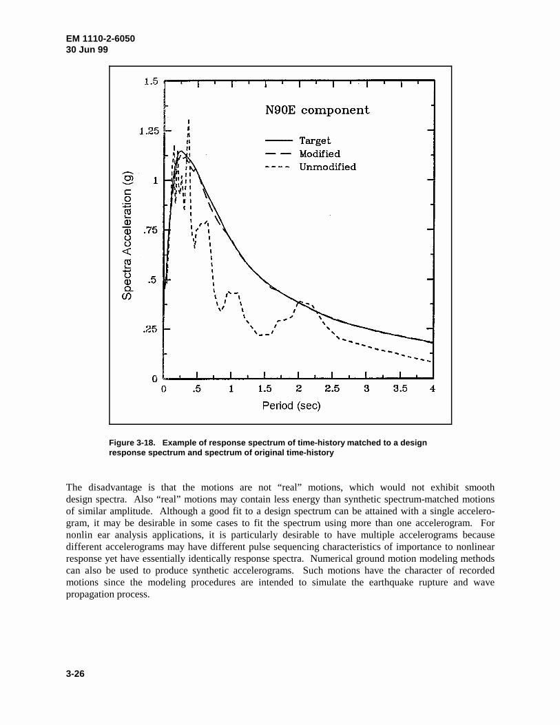
EM 1110-2-605030 Jun 99

3-26

Figure 3-18. Example of response spectrum of time-history matched to a designresponse spectrum and spectrum of original time-history

The disadvantage is that the motions are not “real” motions, which would not exhibit smoothdesign spectra. Also “real” motions may contain less energy than synthetic spectrum-matched motionsof similar amplitude. Although a good fit to a design spectrum can be attained with a single accelero-gram, it may be desirable in some cases to fit the spectrum using more than one accelerogram. Fornonlin ear analysis applications, it is particularly desirable to have multiple accelerograms becausedifferent accelerograms may have different pulse sequencing characteristics of importance to nonlinearresponse yet have essentially identically response spectra. Numerical ground motion modeling methodscan also be used to produce synthetic accelerograms. Such motions have the character of recordedmotions since the modeling procedures are intended to simulate the earthquake rupture and wavepropagation process.

EM 1110-2-605030 Jun 99

3-27

3-7. Developing Site-Specific Spectra for Soil Sites

As is the case for developing site-specific rock spectra, either the approach of anchoring spectral shapesto a peak ground acceleration (Approach 1) or the approach of directly estimating the spectra(Approach 2) can be used for soil sites. The implementation of these approaches is outlined below.

a. Approach 1 - Anchoring the response spectral shape to the peak ground acceleration.

(1) Estimating peak ground acceleration. Table 3-1 summarizes recently developed attenuation rela-tionships for estimating peak ground acceleration. For WUS shallow crustal faulting earthquakes,several recent attenuation relationships are available to estimate top-of-soil peak ground accelerations forfirm soil conditions, and Idriss (1991a) has developed a peak acceleration attenuation relationship forsoft soil sites. Combining the BLWN/RVT method for rock motion estimation with a site responseanalysis for a deep soil column, Boore and Joyner (1991) developed a peak ground accelerationattenuation relationship for deep soil sites in the EUS. For subduction zone earthquakes, attenuationrelationships have been developed for firm soil conditions and in some cases for soft soil conditions(Table 3-1). As is the case for rock attenuation relationships, the soil attenuation relationships are betterconstrained by data for WUS shallow crustal earthquakes than for EUS or subduction zone earthquakes.

(2) Estimating response spectral shape and the response spectrum. Spectral shapes that have beendeveloped for soil sites for WUS shallow crustal earthquakes and for subduction zone earthquakes on thebasis of statistical analyses of ground motion data are summarized in Table 3-2. Spectral shapes have notbeen developed for soil sites for EUS earthquakes. Using the Newmark and Hall (1978, 1982) approach(Appendix B), the effect of soil is accounted for by estimating values of peak ground velocity and peakground displacement directly, or by using Newmark and Hall’s relationships between peak groundacceleration, peak ground velocity, and peak ground displacement for firm soil to estimate peak groundvelocity and peak ground displacement, given peak ground acceleration. Peak ground acceleration,velocity, and displacement then are multiplied by Newmark and Hall’s amplification factors to obtain theabsolute response spectrum.

(3) Uncertainty in response spectra predictions. The comments made in paragraph 3-6a(3) regardingestimating 84th percentile response spectra for rock also apply to response spectra for soil.

(4) Estimating vertical ground motion response spectra. Recent studies (e.g., Silva 1997) indicatethat vertical-to-horizontal ratios of response spectra of ground motions are higher on soil than on rock forshort periods of vibration. Figure 3-16 provides a guideline for ratios of vertical-to-horizontal spectralratios on firm soil sites that is generally conservative. However, if a facility is sensitive to short-period(less than 0.3 sec) vertical motions, and is located within 25 km of the earthquake source or themagnitude exceeds 6.5, further evaluation of vertical response spectra on soil is recommended becausevertical response spectra can significantly exceed horizontal response spectra for these conditions.

b. Using Approach 2 - Estimating the soil response spectrum directly.

(1) General. The three approaches discussed in paragraph 3-5b can be used for soil sites. Theseapproaches are using response spectral attenuation relationships, performing statistical analysis of groundmotion response spectra, and theoretical (numerical) modeling.

(2) Using response spectral attenuation relationships. Recently developed response spectralattenuation relationships for soil are summarized in Table 3-3. The spectral attenuation relationships in

EM 1110-2-605030 Jun 99

3-28

Table 3-3 generally include the standard deviations of the estimates, from which 84th percentile valuesmay be obtained.

(3) Using statistical analyses of response spectra. Abundant ground motion data for firm soil sites inthe WUS are available to permit statistical analyses of data sets for many design earthquakes. Althoughsuch data are not available for EUS earthquakes, the WUS data can be used, recognizing that the analysesmay underestimate short-period (less than 0.1 to 0.3 sec) response spectra. (Refer to discussion for rocksites in paragraph 3-6b(3).) The degree of underestimation should be less at soil sites than at rock sitesbecause soils will tend to damp out the short-period motions.

(4) Using theoretical (numerical) modeling techniques. The techniques discussed in para-graph 3-5b(3) can be used to simulate the earthquake rupture and propagation of seismic waves from theearthquake source to the site. In addition, site response analyses may be carried out to estimate top-of-soil response spectra, given a response spectrum in rock. With this approach, rock motions, includingresponse spectra, are first defined for the site (using procedures and relationships described in para-graph 3-6). The soil profile between the ground surface and the underlying rock is modeled. The rockmotions are assigned to a hypothetical rock outcrop at the site rather than to the rock at depth beneath thesoil column. This is because rock motion recordings are obtained at the ground surface rather than atdepth, and unless the rock is rigid, the rock motion beneath the soil column will differ somewhat from therock outcrop motion. Then, using nonlinear or equivalent linear soil response analytical methods, rockmotions are propagated through the soils column and top-of-soil motions are estimated. The siteresponse analysis process is schematically illustrated in Figure 3-19. This figure illustrates thecommonly used one-dimensional site response analysis method applicable where the soil stratigraphy isrelatively uniform and flat-lying and the ground surface topography is relatively level. Two-dimensionalsite response analysis methods are available for situations where these conditions are not sufficientlymet. Just as in other types of theoretical modeling and numerical analyses, results of site responseanalyses are sensitive to the details of the analytical procedures, modeling of the process, and inputs tothe analysis. Broad guidelines for conducting these analyses are listed below:

(a) More than one input rock acceleration time-history should be used, and the selected motionsshould be reasonably representative of the rock motions in terms of spectra and duration.

(b) Parametric analyses for variations in the dynamic soil properties should be made to examine thesensitivity of the response to uncertainties in the soil properties. This is particularly important when soilproperties are based on generalized correlations rather than on a program of field shear wave velocitymeasurements.

(c) It is useful to compute ratios of response spectra of top-of-soil motion to input rock motion foreach analysis that is carried out. The ratios are much less sensitive to the actual input motion than is theabsolute top-of-soil motion. The spectral ratios can then be examined and smoothed and multiplied bythe rock smooth spectrum to obtain a top-of-soil spectrum, which can be further smoothed.

An illustration of a site response analysis is presented in Appendix E. Articles by Seed and Sun (1989),Chang et al. (1990), and Ahmad, Gazetas, and Desai (1991) provide useful background information onsite response analysis methodologies. Site response analyses are needed relatively more for soft soil sitesthan for firm soil sites because the site response effects are greater for soft soils and because groundmotion data and empirically based ground motion relationships are relatively scarce for soft soil sites.

EM 1110-2-605030 Jun 99

3-29

Figure 3-19. Schematic of one-dimensional siteresponse analysis

(5) Estimating vertical ground motion response spectra. The available recently developedattenuation relationships for response spectral accelerations of vertical firm-soil site motions aresummarized in Table 3-3. These relationships can be used directly to estimate vertical response spectraon firm soils sites. The vertical to horizontal response spectral ratios discussed in paragraph 3-7a(4) andshown in Figure 3-16 can be used as a guide in estimating vertical response spectra, given an estimate ofhorizontal response spectra.

c. Developing acceleration time-histories of soil motions consistent with design response spectrum.The two alternatives for developing acceleration time-histories for rock motions that were discussed in

pE(z) 1 e(�z # t)

EM 1110-2-605030 Jun 99

3-30

paragraph 3-6c, namely, selecting recorded motions and synthetically developing or modifying motions,can also be used to develop time-histories for top-of-soil motions. In the case where site responseanalyses are carried out to define top-of-soil motions, there is a third alternative, which is to obtain thetime-histories directly from the site response analyses.

Section IIIProbabilistic Approach for Developing Site-Specific Response Spectra

3-8. Overview of Probabilistic Seismic Hazard Analysis (PSHA) Methodology

a. General. PSHA takes the elements of a deterministic assessment of earthquake ground shakinghazard—identification of seismic sources; specification of limiting earthquake sizes; assessment ofground motions as a function of earthquake magnitude; source-to-site distance; and site conditions—andadds an assessment of the likelihood that ground shaking will occur during a specified time period. Fig-ure 3-20 shows a typical result of PSHA, termed a hazard curve, that relates the level of ground shakingto the annual frequency of exceedance of that level. The ground motion parameter for the example inFigure 3-20 is peak ground acceleration. PSHA may be conducted for other ground motion parameters,such as peak ground velocity or response spectral values for specific periods of vibration and dampingratios. If a PSHA is carried out for response spectral values at a number of periods of vibration, thenresponse spectra having selected probabilities of exceedance (i.e., “equal hazard” response spectra) maybe constructed, as will be discussed later.

b. Elements of a PSHA. Evaluation of the frequency or probability of exceedance of groundmotions at a site is a function of earthquake source definition (distance of the sources from the site,source geometries, and frequencies of occurrence (recurrence) of earthquakes of different magnitudes oneach source), and ground motion attenuation (amplitudes of ground motion as a function of earthquakemagnitude and distance). These basic inputs to a PSHA are then combined in a probabilistic model toobtain hazard curves and (if desired) equal-hazard response spectra as discussed above. The basicelements of a PSHA are illustrated in Figure 3-21 for peak ground acceleration and in Figure 3-22 forequal hazard response spectra.

c. Formulation of PSHA methodology.

(1) Formulation. The methodology used to conduct PSHA was initially developed by Cornell(1968). Current practice is described in several publications, such as National Research Council (1988)and Earthquake Engineering Research Institute Committee on Seismic Risk (1989). Using a Poissonprobability model (paragraph 3-9d), the probability of exceedance p (z) of a ground motion level z in anE

exposure time or design time period t at a site is related to the annual frequency of ground motionexceedance at the site, � , by:z

(3-1)

A PSHA is carried out to obtain � , and p (z) can then be obtained using Equation 3-1. The return periodz E

(RP) for ground motion exceedance at a site is equal to the reciprocal of � . The results of a PSHA are,z

in practice, expressed in terms of one or more of the parameters, p (z), � , and RP. Using Equation 3-1,E z

the interrelationship between these fundamental parameters is illustrated in graphical form in Figure 3-23and in tabular form in Table 3-4. Note that when (� •t) is small (approximately � 0.1), p (z) isz E

approximately equal to � •t. For larger values of � •t, p (z) is less than (� •t). The basic formulation forz z E z

� is:z

vz�N�M� (mi) •�

RP (Rrj |mi) • P (Z > z mi rj)

n

�N

EM 1110-2-605030 Jun 99

3-31

Figure 3-20. Example seismic hazard curve showing relationship between peak groundacceleration and probability (annual frequency) of exceedance

(3-2)

where

= summation over all (N) seismic sources

�(m ) = the annual frequency of occurrence of earthquakes of magnitude m (above a certaini i

minimum size of engineering significance) on seismic source n

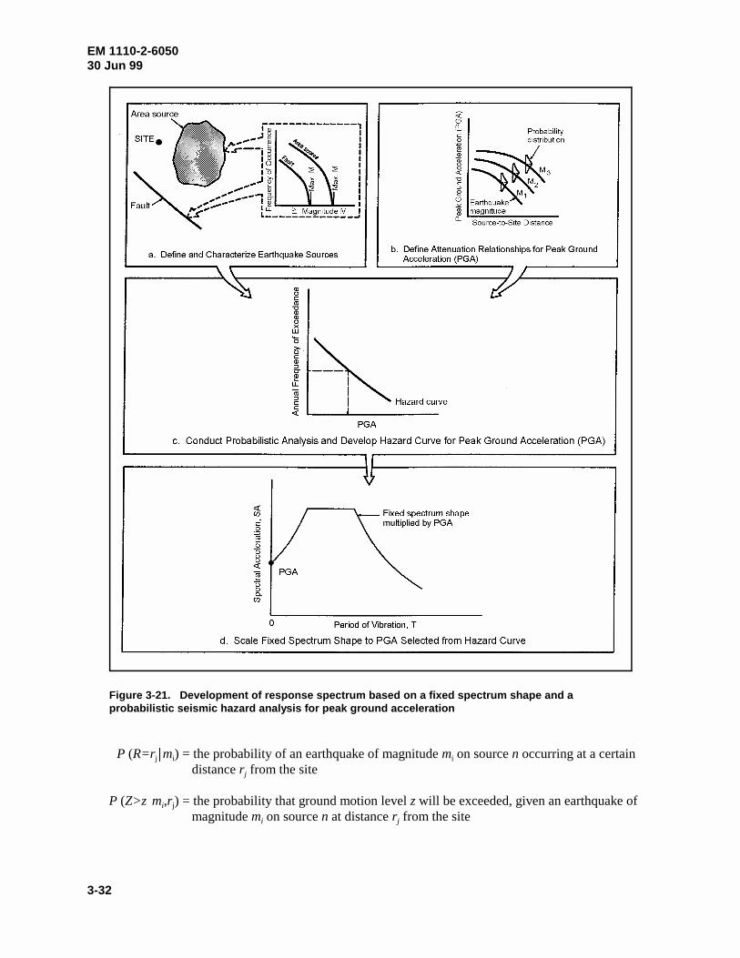
EM 1110-2-605030 Jun 99

3-32

Figure 3-21. Development of response spectrum based on a fixed spectrum shape and aprobabilistic seismic hazard analysis for peak ground acceleration

P (R=r m ) = the probability of an earthquake of magnitude m on source n occurring at a certainj i i

distance r from the sitej

P (Z>z m ,r ) = the probability that ground motion level z will be exceeded, given an earthquake ofi j

magnitude m on source n at distance r from the sitei j

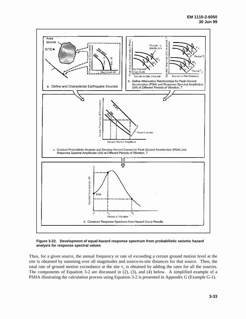
EM 1110-2-605030 Jun 99

3-33

Figure 3-22. Development of equal-hazard response spectrum from probabilistic seismic hazardanalysis for response spectral values

Thus, for a given source, the annual frequency or rate of exceeding a certain ground motion level at thesite is obtained by summing over all magnitudes and source-to-site distances for that source. Then, thetotal rate of ground motion exceedance at the site � is obtained by adding the rates for all the sources.z

The components of Equation 3-2 are discussed in (2), (3), and (4) below. A simplified example of aPSHA illustrating the calculation process using Equation 3-2 is presented in Appendix G (Example G-1).

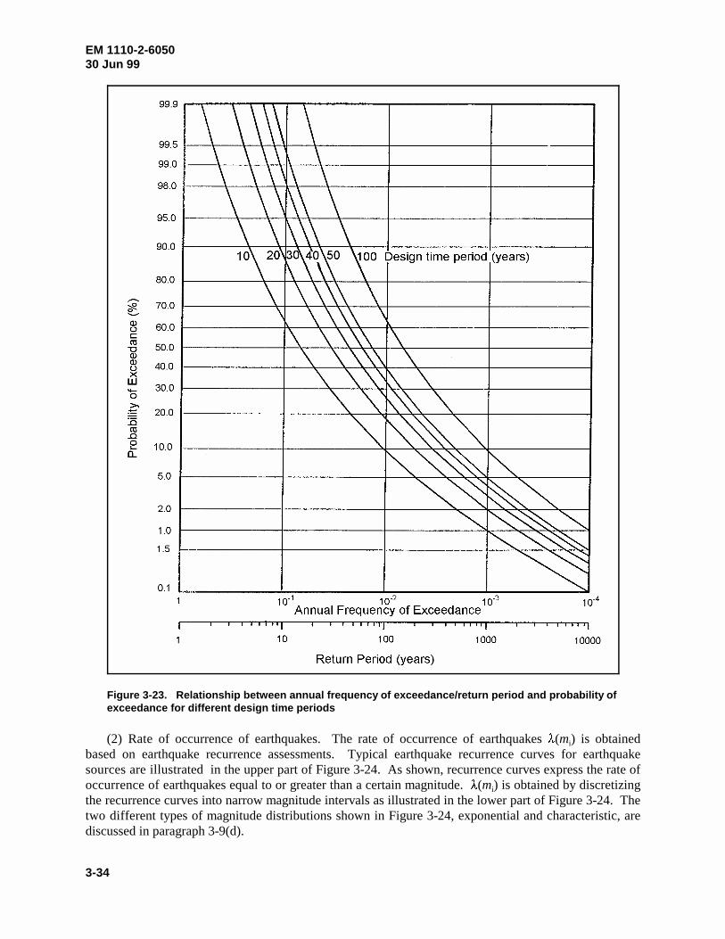
EM 1110-2-605030 Jun 99

3-34

Figure 3-23. Relationship between annual frequency of exceedance/return period and probability ofexceedance for different design time periods

(2) Rate of occurrence of earthquakes. The rate of occurrence of earthquakes �(m ) is obtainedi

based on earthquake recurrence assessments. Typical earthquake recurrence curves for earthquakesources are illustrated in the upper part of Figure 3-24. As shown, recurrence curves express the rate ofoccurrence of earthquakes equal to or greater than a certain magnitude. �(m ) is obtained by discretizingi

the recurrence curves into narrow magnitude intervals as illustrated in the lower part of Figure 3-24. Thetwo different types of magnitude distributions shown in Figure 3-24, exponential and characteristic, arediscussed in paragraph 3-9(d).

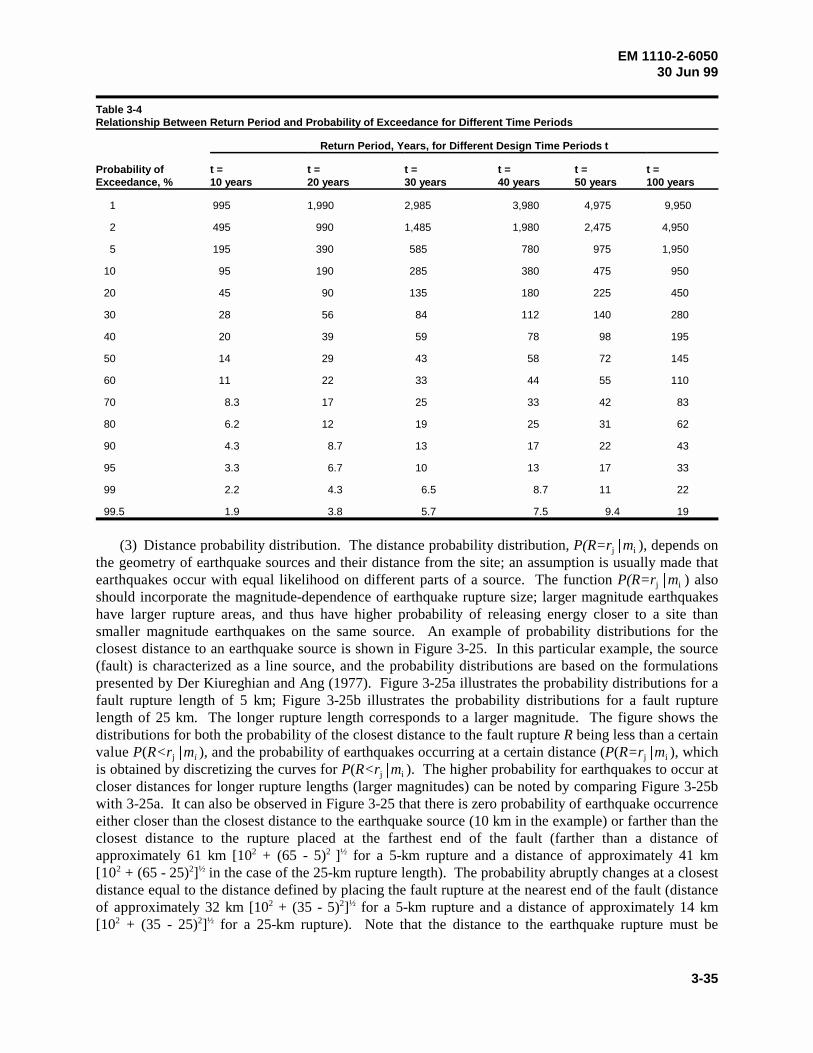
EM 1110-2-605030 Jun 99

3-35

Table 3-4Relationship Between Return Period and Probability of Exceedance for Different Time Periods

Return Period, Years, for Different Design Time Periods t

Probability of t = t = t = t = t = t =Exceedance, % 10 years 20 years 30 years 40 years 50 years 100 years

1 995 1,990 2,985 3,980 4,975 9,950

2 495 990 1,485 1,980 2,475 4,950

5 195 390 585 780 975 1,950

10 95 190 285 380 475 950

20 45 90 135 180 225 450

30 28 56 84 112 140 280

40 20 39 59 78 98 195

50 14 29 43 58 72 145

60 11 22 33 44 55 110

70 8.3 17 25 33 42 83

80 6.2 12 19 25 31 62

90 4.3 8.7 13 17 22 43

95 3.3 6.7 10 13 17 33

99 2.2 4.3 6.5 8.7 11 22

99.5 1.9 3.8 5.7 7.5 9.4 19

(3) Distance probability distribution. The distance probability distribution, P(R=r m ), depends onj i

the geometry of earthquake sources and their distance from the site; an assumption is usually made thatearthquakes occur with equal likelihood on different parts of a source. The function P(R=r m ) alsoj i

should incorporate the magnitude-dependence of earthquake rupture size; larger magnitude earthquakeshave larger rupture areas, and thus have higher probability of releasing energy closer to a site thansmaller magnitude earthquakes on the same source. An example of probability distributions for theclosest distance to an earthquake source is shown in Figure 3-25. In this particular example, the source(fault) is characterized as a line source, and the probability distributions are based on the formulationspresented by Der Kiureghian and Ang (1977). Figure 3-25a illustrates the probability distributions for afault rupture length of 5 km; Figure 3-25b illustrates the probability distributions for a fault rupturelength of 25 km. The longer rupture length corresponds to a larger magnitude. The figure shows thedistributions for both the probability of the closest distance to the fault rupture R being less than a certainvalue P(R<r m ), and the probability of earthquakes occurring at a certain distance (P(R=r m ), whichj i j i

is obtained by discretizing the curves for P(R<r m ). The higher probability for earthquakes to occur atj i

closer distances for longer rupture lengths (larger magnitudes) can be noted by comparing Figure 3-25bwith 3-25a. It can also be observed in Figure 3-25 that there is zero probability of earthquake occurrenceeither closer than the closest distance to the earthquake source (10 km in the example) or farther than theclosest distance to the rupture placed at the farthest end of the fault (farther than a distance ofapproximately 61 km [10 + (65 - 5) ] for a 5-km rupture and a distance of approximately 41 km2 2 ½

[10 + (65 - 25) ] in the case of the 25-km rupture length). The probability abruptly changes at a closest2 2 ½

distance equal to the distance defined by placing the fault rupture at the nearest end of the fault (distanceof approximately 32 km [10 + (35 - 5) ] for a 5-km rupture and a distance of approximately 14 km2 2 ½

[10 + (35 - 25) ] for a 25-km rupture). Note that the distance to the earthquake rupture must be2 2 ½

EM 1110-2-605030 Jun 99

3-36

Figure 3-24. Typical earthquake recurrence curves and discretized occurrence rates

expressed in terms of the same definition of distance as used in the ground motion attenuation rela-tionships. Typically, some form of closest distance to rupture definition is used for attenuation relation-ships (variations in this definition include closest distance to rupture, closest distance to rupture of theseismogenic zone, closest horizontal distance to surface projection of rupture, etc.).

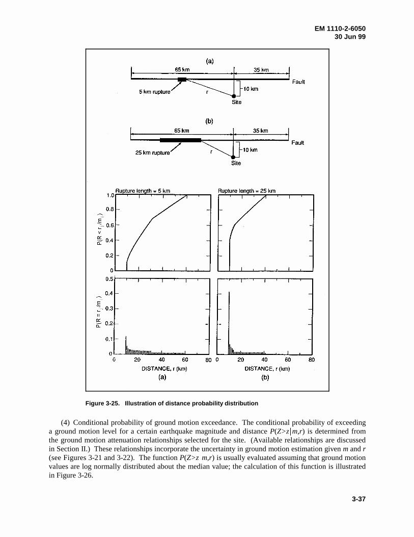
EM 1110-2-605030 Jun 99

3-37

Figure 3-25. Illustration of distance probability distribution

(4) Conditional probability of ground motion exceedance. The conditional probability of exceedinga ground motion level for a certain earthquake magnitude and distance P(Z>z m,r) is determined fromthe ground motion attenuation relationships selected for the site. (Available relationships are discussedin Section II.) These relationships incorporate the uncertainty in ground motion estimation given m and r(see Figures 3-21 and 3-22). The function P(Z>z m,r) is usually evaluated assuming that ground motionvalues are log normally distributed about the median value; the calculation of this function is illustratedin Figure 3-26.

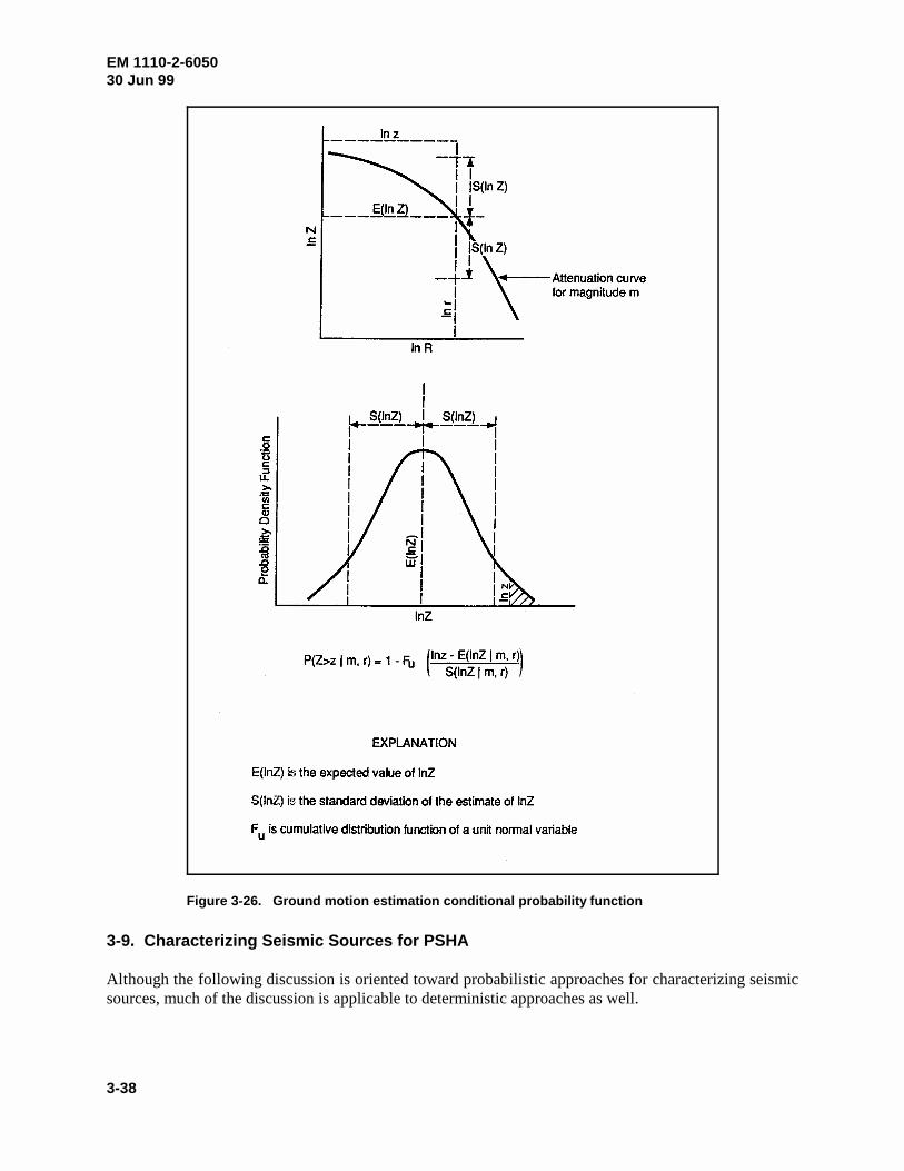
EM 1110-2-605030 Jun 99

3-38

Figure 3-26. Ground motion estimation conditional probability function

3-9. Characterizing Seismic Sources for PSHA

Although the following discussion is oriented toward probabilistic approaches for characterizing seismicsources, much of the discussion is applicable to deterministic approaches as well.

EM 1110-2-605030 Jun 99

3-39

a. Source identification.

(1) Seismic source. A seismic source represents a region of the earth's crust where thecharacteristics of earthquake activity are recognized to be different from those of the adjacent crust.Seismic sources are identified on the basis of geological, seismological, and geophysical data. An under-standing of the regional tectonics, local Quaternary geologic history, and seismicity of an area leads tothe identification of seismic sources. The development of tectonic models for crustal deformation andthe assessment of the tectonic role of individual geologic structures are useful for both identifyingpotential sources and assessing their characteristics. Geologic studies can be used to assess the location,timing, and style of crustal deformation. The association of geologic structures with historic or instru-mental seismicity may clarify their role within the present tectonic stress regime. Characteristics ofseismicity, including epicenter locations, focal depths, and source mechanisms, also aid in identifyingpotential sources.

(2) Faults. Because earthquakes occur as a result of differential slip on faults, modeling of seismicsources as individual faults is the most physically realistic model for seismic hazard analysis. Underfavorable conditions, individual faults can be identified and treated as distinct seismic sources. Activefaults are usually identified on the basis of geomorphic expression and stratigraphic displacements butcan also be identified by lineations of seismicity, by geophysical measurements, or by inference fromdetailed investigations of related geologic structures, such as active folding or crustal plate subduction.A fault model for individual sources allows the use of geologic data on fault behavior, as well asseismicity data, to characterize earthquake activity.

(3) Seismic source zones. In areas with low rates of crustal deformation away from plate margins,such as the EUS, seismic sources are often defined as seismic source zones. Seismic source zones areused to model the occurrence of seismicity in areas where specific faults cannot be identified and wherethe observed seismicity exhibits a diffuse pattern not clearly associated with individual faults. Theseconditions are typical of areas with lower rates of crustal deformation, such as regions away from platemargins (e.g., EUS). Seismic source zones can be defined based either on historical seismicity patternsor geology and tectonics. When defined based on historical seismicity patterns, a large region can besubdivided into small regular areas that are treated as individual source zones (Electric Power ResearchInstitute (EPRI) 1987; U.S. Geological Survey (USGS) 1996). With this approach, it is assumed that thespatial variation in the occurrence rate of future earthquakes is similar to the historical pattern ofseismicity. Due to the relatively short historical period and low rates of seismicity, the seismicitypatterns are usually determined by small earthquakes. It is not clear whether this pattern reflects thelikelihood of future earthquakes of engineering significance (generally taken to be earthquakes ofmagnitude approximately equal to or greater than 5). The alternative approach is to define areas thoughtto have homogeneous earthquake potential characteristics (in terms of rate of earthquake occurrence andmaximum earthquake size) on the basis of the geology and tectonics of the region. For example, recentevidence from studies of global earthquakes in stable continental regions such as the EUS has shown thatmost larger earthquakes occur through reactivation of faults in geologically ancient rift zones (Johnstonet al. 1994). Where available, paleoseismological data (e.g., spatial and temporal distribution ofliquefaction features) should be used to identify source regions for large-magnitude earthquakes.Because of uncertainty regarding the most appropriate model for earthquake occurrence, both seismicity-based and geologically based seismic source zones should be included in a probabilistic analysis.

b. Source geometry.

(1) General. Description of the geometry of a seismic source is necessary to evaluate the distancesfrom the site at which future earthquakes could occur. In addition, source geometry can place physicalconstraints on the maximum size earthquake that can occur on a source.

EM 1110-2-605030 Jun 99

3-40

(2) Faults. Seismic sources defined as faults are modeled in a PSHA as segmented linear or planarfeatures. Earthquake ruptures on fault sources are modeled as rupture lengths or rupture areas, with thesize of rupture defined on the basis of empirical relationships between earthquake magnitude and rupturesize (Wyss 1979; Wells and Coppersmith 1993).

(3) Seismic source zones. For seismic sources defined as geologic structures suspected to containfaults, the distribution of earthquakes can be modeled as rupture surfaces occurring on multiple faultplanes distributed throughout the source volume if the general trend of such planes is known or can beinferred. Alternatively, earthquake locations can be modeled as random point sources within the sourcevolume if the orientation of potential fault planes is unknown. The spatial distribution of seismicitywithin large areal sources can be modeled similarly.

c. Maximum earthquake magnitude.

(1) Faults. The limiting size earthquake that can occur on each seismic source is an importantparameter, especially in evaluating seismic hazard at low probability levels. The maximum magnitudecan most easily be estimated when the seismic source is defined on the basis of an identifiable fault. Forfaults, the maximum earthquake magnitude is related to fault geometry and fault behavior through anassessment of the maximum dimensions of a single rupture. Evaluation of fault segmentation can play akey role in identifying portions of a fault zone likely to represent the largest size of a single rupture(Schwartz and Coppersmith 1986; Schwartz 1988). The maximum magnitude is related to the maximumrupture size through empirical relationships (Slemmons 1982; Bonilla, Mark, and Lienkaemper 1984;Wells and Coppersmith 1994). Because these relationships are subject to uncertainty, the use of anumber of magnitude estimation techniques can result in more reliable estimates of maximum magnitudethan the application of a single relationship.

(2) Seismic source zones. The assessment of maximum magnitude is more difficult when seismicsources are defined on the basis of large-scale tectonic features or crustal blocks, as is typically done inthe EUS. In such cases the maximum magnitude is often estimated to be the maximum historicalearthquake magnitude plus an increment, or is estimated to be a magnitude having a specified returnperiod. The chief weakness of these approaches is the generally short period of historical observationscompared with the likely return period of a maximum event for an individual source. Another approachthat attempts to extend the generally short observational period for individual sources is based inaugmenting the assessment using data from analogous structures worldwide. This approach identifiesanalogous features for which the maximum magnitude is better defined or identifies the largest event thathas occurred on such features. In the application of analogies, the seismicity of similar structures on aworldwide basis can be examined to supplement the limited local historical record. Recent efforts havebeen made to use a global earthquake database to identify the factors that control or limit the maximumsize of earthquakes within stable continental regions like the EUS to develop a formal method forestimating maximum magnitude in such regions (Johnston et al. 1994)

d. Rate of earthquake occurrence and distribution in earthquake size.

(1) Estimating recurrence rates. Earthquake recurrence rates are estimated from historicalseismicity, from geological data on rates of fault movement, and from paleoseismic data on the timing oflarge prehistoric events. For areal sources, historical seismicity is usually used to estimate earthquakerecurrence rates. When recurrence for small, regular source zones (cells) is analyzed (a(3) above),procedures can be employed to smooth seismicity rates among adjoining cells (EPRI 1987; USGS 1996).In an analysis of the earthquake catalog of historical seismicity, it is important to translate the data into acommon magnitude scale consistent with the magnitude scale used in the ground motion attenuation

EM 1110-2-605030 Jun 99

3-41

relationships, and to account for completeness in earthquake reporting as a function of time and location.Straightforward statistical techniques can then be used to estimate earthquake recurrence parameters(Weichert 1980).

(2) Use of geologic data for faults. For sources defined as individual faults, the available historicalseismicity is usually insufficient to characterize the earthquake recurrence. Geologic data on fault sliprates can be used to estimate the rate of seismic moment release, leading to the rate of earthquake recur-rence. In addition, paleoseismic studies of the occurrence of large prehistoric events can be used toestimate recurrence of larger magnitude earthquakes on a fault. Predictions of recurrence rates for largerevents from fault-specific geologic data have been shown to match well with observed historical rates ona regional basis (Youngs and Coppersmith 1985b; Youngs, Swan, and Power 1988; Youngs et al. 1987;Youngs et al. 1993b). The rate of earthquake occurrence may not be uniform along the strike or dip of anearthquake fault. Evaluation of fault segmentation can be used to characterize variations in recurrencealong the length of a fault. The depth distribution of historical seismicity can be used to specify down-dip variations in recurrence.

(3) Recurrence models. The relative frequency of various size earthquakes has usually beenspecified by the truncated exponential recurrence model (Cornell and Van Marke 1969) based onGutenberg and Richter's (1954) recurrence law. This model was developed on the basis of observationsof global seismicity. It has been found to work well on a regional basis and for modeling seismicity fornonfault specific sources such as distributed seismicity zones and generalized tectonic structures. Recentadvances in understanding of the earthquake generation process have indicated that earthquakerecurrence on individual faults may not conform to the exponential model. Instead, individual faults orfault segments may tend to rupture in what have been termed “characteristic” magnitude events at or nearthe maximum magnitude (Schwartz and Coppersmith 1984). This has led to the development of fault-specific recurrence models such as the maximum moment model (Wesnousky et al. 1983) and thecharacteristic magnitude recurrence model (Youngs and Coppersmith 1985a, 1985b). Figure 3-27 illus-trates a characteristic magnitude recurrence model. Figure 3-28 compares exponential and characteristicearthquake recurrence relationships. The figure illustrates the differences between the two recurrencemodels depending on how the earthquake recurrence rate is specified. Figure 3-28a shows recurrencecurves if the total rate of seismic moment release is specified to be the same for each model;Figure 3-28b shows recurrence curves if the rate of large-magnitude earthquakes is specified to be thesame for each model. Detailed studies of earthquake recurrence in the Wasatch fault region, Utah, and inthe San Francisco Bay region have shown excellent matches between regional seismicity rates and recur-rence modeling when combining the characteristic recurrence model for individual faults with theexponential model for distributed source areas (Youngs et al. 1987; Youngs, Swan, and Power 1988;Youngs et al. 1993b).

(4) Poisson versus real-time recurrence. Nearly all PSHA's assume that earthquake occurrence intime is a random and memoryless (Poisson) process. In the Poisson process, it is assumed that theprobability of an event in a specified period is completely determined by the average frequency ofoccurrence of events, and the probability of occurrence of the next event is independent of when the lastevent occurred. While the observed seismicity data on a regional basis have been shown to be consistentwith the Poisson model, the model does not conform to the physical process believed to result inearthquakes, one of a gradual, relatively uniform rate of strain accumulation followed by sudden release.Detailed paleoseismic studies of several faults as well as historical seismicity from very activesubduction zones have indicated that the occurrence of the larger events on a source tends to be morecyclic in nature. These observations have led to the use of nonstationary or “real-time” recurrencemodels that predict the probability of events in the next period, rather than any period. Typically, a

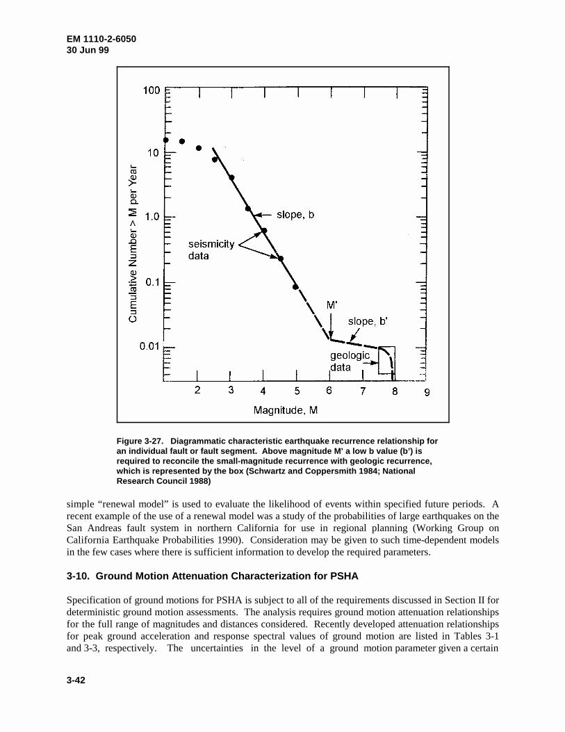
EM 1110-2-605030 Jun 99

3-42

Figure 3-27. Diagrammatic characteristic earthquake recurrence relationship foran individual fault or fault segment. Above magnitude M’ a low b value (b’) isrequired to reconcile the small-magnitude recurrence with geologic recurrence,which is represented by the box (Schwartz and Coppersmith 1984; NationalResearch Council 1988)

simple “renewal model” is used to evaluate the likelihood of events within specified future periods. Arecent example of the use of a renewal model was a study of the probabilities of large earthquakes on theSan Andreas fault system in northern California for use in regional planning (Working Group onCalifornia Earthquake Probabilities 1990). Consideration may be given to such time-dependent modelsin the few cases where there is sufficient information to develop the required parameters.

3-10. Ground Motion Attenuation Characterization for PSHA

Specification of ground motions for PSHA is subject to all of the requirements discussed in Section II fordeterministic ground motion assessments. The analysis requires ground motion attenuation relationshipsfor the full range of magnitudes and distances considered. Recently developed attenuation relationshipsfor peak ground acceleration and response spectral values of ground motion are listed in Tables 3-1and 3-3, respectively. The uncertainties in the level of a ground motion parameter given a certain

EM 1110-2-605030 Jun 99

3-43

Figure 3-28. Comparison of truncated exponential and characteristic earthquake recurrencerelationships

earthquake magnitude and distance (modeled by the probability distribution for the attenuationrelationship (Figure 3-26)) are of considerable importance in influencing the results of a PSHA andshould be included in the analysis.

3-11. Treatment of Scientific Uncertainty in PSHA

The basic probability formulations in Equations 3-1 and 3-2 incorporate the randomness of the physicalprocess of earthquake generation and seismic wave propagation. Although these formulationsincorporate the inherent uncertainty due to randomness, they do not incorporate additional sources ofuncertainty that may be associated with the choice of particular models or model parameters. Forexample, there could be uncertainty about which ground motion attenuation relationship is mostapplicable to a site, whether an exponential or characteristic earthquake recurrence model is mostapplicable, the most appropriate model for seismic source zones, the geometry of earthquake sources, thevalues of maximum earthquake magnitude, or earthquake recurrence parameters. In a deterministicanalysis, these uncertainties, which are termed scientific or epistemic uncertainties, are usually treated byapplying conservatism in selecting design earthquakes and estimating ground motions. In PSHA, theseuncertainties can be directly modeled within the analysis framework to provide an assessment of theuncertainty in the result. The technique of “logic trees” has been widely used to incorporate scientificuncertainty in a PSHA (Kulkarni, Youngs, and Coppersmith 1984; Youngs et al. 1985; Coppersmith andYoungs 1986; National Research Council 1988). Figure 3-29 shows an example of a logic tree used in aPSHA. Although only a few branches of the logic tree are shown, there may be many thousands ofbranches in the tree. Each path through the tree to an end branch (on the right side of Figure 3-29)

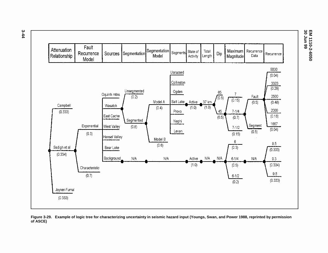
EM

1110-2-605030 Ju

n 99

3-44

Figure 3-29. Example of logic tree for characterizing uncertainty in seismic hazard input (Youngs, Swan, and Power 1988, reprinted by permissionof ASCE)

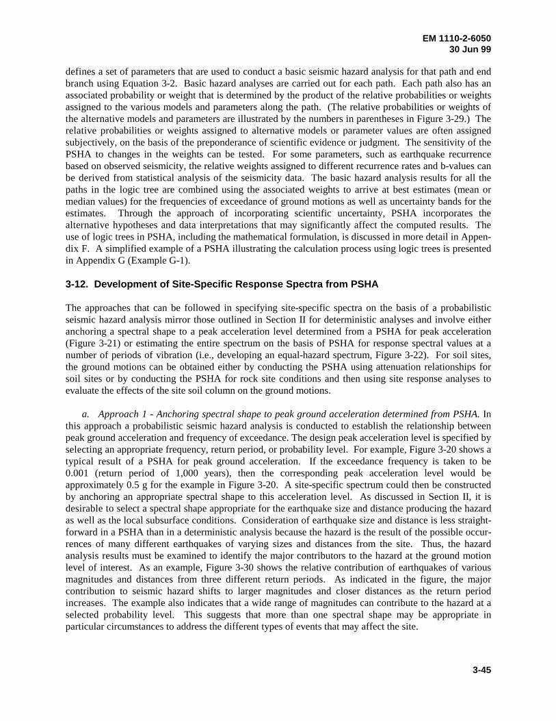
EM 1110-2-605030 Jun 99

3-45

defines a set of parameters that are used to conduct a basic seismic hazard analysis for that path and endbranch using Equation 3-2. Basic hazard analyses are carried out for each path. Each path also has anassociated probability or weight that is determined by the product of the relative probabilities or weightsassigned to the various models and parameters along the path. (The relative probabilities or weights ofthe alternative models and parameters are illustrated by the numbers in parentheses in Figure 3-29.) Therelative probabilities or weights assigned to alternative models or parameter values are often assignedsubjectively, on the basis of the preponderance of scientific evidence or judgment. The sensitivity of thePSHA to changes in the weights can be tested. For some parameters, such as earthquake recurrencebased on observed seismicity, the relative weights assigned to different recurrence rates and b-values canbe derived from statistical analysis of the seismicity data. The basic hazard analysis results for all thepaths in the logic tree are combined using the associated weights to arrive at best estimates (mean ormedian values) for the frequencies of exceedance of ground motions as well as uncertainty bands for theestimates. Through the approach of incorporating scientific uncertainty, PSHA incorporates thealternative hypotheses and data interpretations that may significantly affect the computed results. Theuse of logic trees in PSHA, including the mathematical formulation, is discussed in more detail in Appen-dix F. A simplified example of a PSHA illustrating the calculation process using logic trees is presentedin Appendix G (Example G-1).

3-12. Development of Site-Specific Response Spectra from PSHA

The approaches that can be followed in specifying site-specific spectra on the basis of a probabilisticseismic hazard analysis mirror those outlined in Section II for deterministic analyses and involve eitheranchoring a spectral shape to a peak acceleration level determined from a PSHA for peak acceleration(Figure 3-21) or estimating the entire spectrum on the basis of PSHA for response spectral values at anumber of periods of vibration (i.e., developing an equal-hazard spectrum, Figure 3-22). For soil sites,the ground motions can be obtained either by conducting the PSHA using attenuation relationships forsoil sites or by conducting the PSHA for rock site conditions and then using site response analyses toevaluate the effects of the site soil column on the ground motions.

a. Approach 1 - Anchoring spectral shape to peak ground acceleration determined from PSHA. Inthis approach a probabilistic seismic hazard analysis is conducted to establish the relationship betweenpeak ground acceleration and frequency of exceedance. The design peak acceleration level is specified byselecting an appropriate frequency, return period, or probability level. For example, Figure 3-20 shows atypical result of a PSHA for peak ground acceleration. If the exceedance frequency is taken to be0.001 (return period of 1,000 years), then the corresponding peak acceleration level would beapproximately 0.5 g for the example in Figure 3-20. A site-specific spectrum could then be constructedby anchoring an appropriate spectral shape to this acceleration level. As discussed in Section II, it isdesirable to select a spectral shape appropriate for the earthquake size and distance producing the hazardas well as the local subsurface conditions. Consideration of earthquake size and distance is less straight-forward in a PSHA than in a deterministic analysis because the hazard is the result of the possible occur-rences of many different earthquakes of varying sizes and distances from the site. Thus, the hazardanalysis results must be examined to identify the major contributors to the hazard at the ground motionlevel of interest. As an example, Figure 3-30 shows the relative contribution of earthquakes of variousmagnitudes and distances from three different return periods. As indicated in the figure, the majorcontribution to seismic hazard shifts to larger magnitudes and closer distances as the return periodincreases. The example also indicates that a wide range of magnitudes can contribute to the hazard at aselected probability level. This suggests that more than one spectral shape may be appropriate inparticular circumstances to address the different types of events that may affect the site.

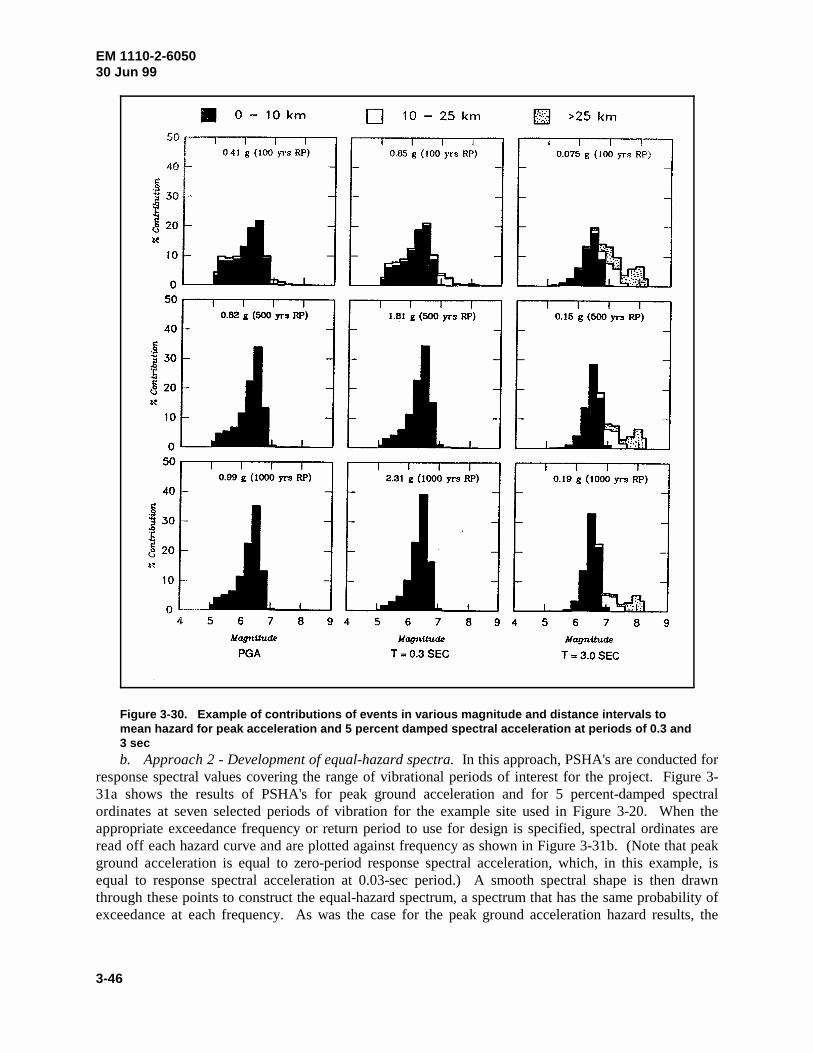
EM 1110-2-605030 Jun 99

3-46

Figure 3-30. Example of contributions of events in various magnitude and distance intervals tomean hazard for peak acceleration and 5 percent damped spectral acceleration at periods of 0.3 and3 secb. Approach 2 - Development of equal-hazard spectra. In this approach, PSHA's are conducted for

response spectral values covering the range of vibrational periods of interest for the project. Figure 3-31a shows the results of PSHA's for peak ground acceleration and for 5 percent-damped spectralordinates at seven selected periods of vibration for the example site used in Figure 3-20. When theappropriate exceedance frequency or return period to use for design is specified, spectral ordinates areread off each hazard curve and are plotted against frequency as shown in Figure 3-31b. (Note that peakground acceleration is equal to zero-period response spectral acceleration, which, in this example, isequal to response spectral acceleration at 0.03-sec period.) A smooth spectral shape is then drawnthrough these points to construct the equal-hazard spectrum, a spectrum that has the same probability ofexceedance at each frequency. As was the case for the peak ground acceleration hazard results, the

EM 1110-2-605030 Jun 99

3-47

Figure 3-31. Construction of equal-hazard spectra. Top plot (a) shows hazardcurves for a range of spectral periods. Bottom plot (b) shows equal hazardspectrum for a period of 1,000 years

EM 1110-2-605030 Jun 99

3-48

equal-hazard spectrum is the result of many possible earthquakes of different sizes and locations. This isillustrated in Figure 3-30, which shows the relative contributions of different magnitude earthquakes tothe hazard as a function of return period for spectral values at two periods of vibration as well as for peakground acceleration. As can be seen, for the same probability of exceedance, the contributions shift tolarger magnitudes as the spectral period of vibration increases. This is because the ground motionattenuation relationships are more strongly a function of magnitude at long periods than short periods ofvibration.

c. Preferred approach. Approach 2 is recommended over Approach 1 because it is not straight-forward to select appropriate spectral shapes in Approach 1. It will be feasible to develop an equal-hazard response spectra from a PSHA using Approach 2. Response spectral value attenuation relation-ships are available for both the EUS and WUS (Section II and Table 3-3) that are as reliable as thosedeveloped for peak ground acceleration. The computation of equal-hazard spectra using these spectralattenuation relationships directly accounts for the changes in contributions to the hazard from differentmagnitudes and source-to-site distances. The use of equal-hazard spectra also accounts for the change inspectral shape with change in return period or probability level, as is illustrated in Figure 3-32 showingan example of equal-hazard response spectral shapes for three probability levels. These are compared inthe figure to a standard spectral shape for a similar site condition.

3-13. Development of Accelerograms

Appropriate accelerograms for use with probabilistically based response spectra can be developed usingthe same two methods described in Section II for deterministic analyses. The additional step required forprobabilistically based response spectra is identification of the appropriate magnitude and distance rangefrom which candidate accelerograms may be selected. This information is obtained by deaggregation ofthe composite hazard to identify the contributions of various magnitudes and distances, as illustrated inFigure 3-30. Suites of natural accelerograms representing the range of events with major contributions tothe hazard may be selected and scaled to approximately correspond to the level of the equal-hazardspectrum. Alternatively, synthetically modified accelerograms can be generated to provide a close matchto the equal-hazard spectrum (paragraph 3-6c).

3-14. Summary of Strengths and Limitations of DSHA and PSHA

a. DSHA.

(1) Strengths.

(a) The concept of the design maximum earthquake (MCE) is straightforward and readilyunderstood by the engineer. The MCE represents an estimate of the maximum earthquake size on asource and is located a defined distance from the site.

(b) Provided an appropriate degree of conservatism is incorporated in defining the earthquakemagnitude, source-to-site distance, and resulting site ground motions, design for the MCE should providean appropriately high level of safety.

(2) Limitations.

(a) The frequency of earthquakes and resulting ground motions is not explicitly considered. As aresult, a deterministic estimate for a maximum earthquake will have a lower probability of beingexceeded in a low-seismicity environment than in a high-seismicity environment.

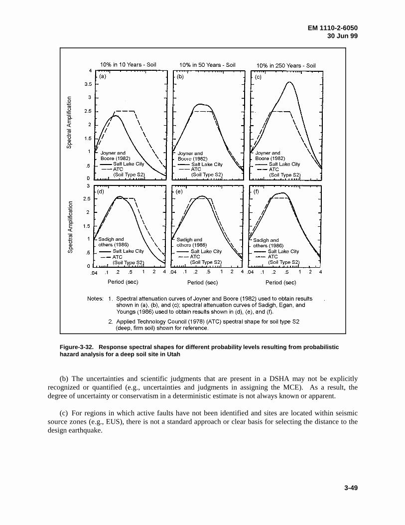
EM 1110-2-605030 Jun 99

3-49

Figure-3-32. Response spectral shapes for different probability levels resulting from probabilistichazard analysis for a deep soil site in Utah

(b) The uncertainties and scientific judgments that are present in a DSHA may not be explicitlyrecognized or quantified (e.g., uncertainties and judgments in assigning the MCE). As a result, thedegree of uncertainty or conservatism in a deterministic estimate is not always known or apparent.

(c) For regions in which active faults have not been identified and sites are located within seismicsource zones (e.g., EUS), there is not a standard approach or clear basis for selecting the distance to thedesign earthquake.

EM 1110-2-605030 Jun 99

3-50

b. PSHA

(1) Strengths.

(a) A PSHA allows the designer to balance risk and cost for a project in a manner similar to thatused for other environmental loadings such as flood or wind loadings. The reduction in risk by selectinga lower probability level (longer return period) and correspondingly higher seismic loading may becompared to the increased project cost involved with designing for the higher loading.

(b) The frequency of occurrence of earthquakes is explicitly incorporated in a PSHA. As such,regions of greater seismic activity (thus higher probabilities of earthquake occurrence) will have higherground motion levels for given probabilities or return periods.

(c) The uncertainty or randomness in earthquake location is explicitly incorporated in a PSHA.Thus, the conservatism of assuming that the earthquake occurs at the closest location on the source to thesite is not necessary in a PSHA. For sites located within low-seismicity seismic source zones in the EUS,it is usually very conservative to “float” the earthquake to the site or even within a small radius of thesite.

(d) Uncertainties in the earthquake occurrence and ground motion estimation process are explicitlyconsidered in a PSHA.

(2) Limitations.

(a) The fact that there are significant scientific uncertainties in earthquake source characterizationand ground motion estimation means that there is not a unique result for the relationship between groundmotion level and probability of exceedance. In fact, there is usually a significant range of possibleground motion levels for a given probability of exceedance. Usually, the mean estimate from a logic treeanalysis is used as a basis for selecting project design criteria.

(b) Probability of exceedance versus ground motion relationships and equal hazard spectra fromPSHA's involve contributions from multiple earthquake sources, magnitudes, and distances. As a result,the concept of a design earthquake is not as straightforward as in a DSHA. Furthermore, the evaluationof the duration of shaking and selection of acceleration time-histories based on probabilistic results aremore difficult than for a deterministic analysis because of the multiple contributions. Therefore, it isimportant to deaggragate the results of a PSHA so that the primary contributors (earthquake sources,magnitude ranges, distance ranges) are known.

(c) While uncertainties are incorporated in the analysis (e.g., by the logic tree approach),nevertheless the weights assigned to alternative models and parameter values generally involvesubjective judgment. The basis for these judgments should be fully documented.

c. Summary. Both deterministic and probabilistic ground motion analyses have their place indeveloping earthquake ground motions for seismic design. These two approaches should be used tocomplement each other as specified in ER 1110-2-1806. It is usually appropriate to carry out both typesof analyses to aid the design engineer in developing the project seismic design criteria. Of paramountimportance in either deterministic or probabilistic analyses is the expertise of the individuals conductingthe analyses.

EM 1110-2-605030 Jun 99

3-51

3-15. Examples of PSHA

Appendix G presents examples of PSHA. The first example is a simplified calculation that illustrates thebasic calculational process and probability functions. The other examples represent actual applicationsin the WUS and EUS. These examples also illustrate how deterministic and probabilistic analyses can beused together in selecting project seismic design ground motions.