DI

SC

US

SI

ON

P

AP

ER

S

ER

IE

S

Forschungsinstitut zur Zukunft der ArbeitInstitute for the Study of Labor

Retaining through Training: Even for Older Workers

IZA DP No. 5591

March 2011

Matteo PicchioJan C. van Ours

Retaining through Training:

Even for Older Workers

Matteo Picchio Tilburg University, CentER, ReflecT

and IZA

Jan C. van Ours Tilburg University, CentER, ReflecT,

University of Melbourne, CESifo, CEPR and IZA

Discussion Paper No. 5591 March 2011

IZA

P.O. Box 7240 53072 Bonn

Germany

Phone: +49-228-3894-0 Fax: +49-228-3894-180

E-mail: iza@iza.org

Any opinions expressed here are those of the author(s) and not those of IZA. Research published in this series may include views on policy, but the institute itself takes no institutional policy positions. The Institute for the Study of Labor (IZA) in Bonn is a local and virtual international research center and a place of communication between science, politics and business. IZA is an independent nonprofit organization supported by Deutsche Post Foundation. The center is associated with the University of Bonn and offers a stimulating research environment through its international network, workshops and conferences, data service, project support, research visits and doctoral program. IZA engages in (i) original and internationally competitive research in all fields of labor economics, (ii) development of policy concepts, and (iii) dissemination of research results and concepts to the interested public. IZA Discussion Papers often represent preliminary work and are circulated to encourage discussion. Citation of such a paper should account for its provisional character. A revised version may be available directly from the author.

IZA Discussion Paper No. 5591 March 2011

ABSTRACT

Retaining through Training: Even for Older Workers* This paper investigates whether on-the-job training has an effect on the employability of workers. Using data from the Netherlands we disentangle the true effect of training incidence from the spurious one determined by unobserved individual heterogeneity. We also take into account that there might be feedback from shocks in the employment status to future propensity of receiving firm-provided training. We find that firm-provided training significantly increases future employment prospects. This finding is robust to a number of robustness checks. It also holds for older workers, suggesting that firm-provided training may be an important instrument to retain older workers at work. JEL Classification: C33, C35, J21, J24, M53 Keywords: training, employment, human capital, older workers Corresponding author: Matteo Picchio Department of Economics Tilburg University PO BOX 90153 5000 LE Tilburg The Netherlands E-mail: m.picchio@uvt.nl

* We acknowledge financial support for this research by Stichting Instituut GAK, through Reflect, the Research Institute for Flexicurity, Labor Market Dynamics and Social Cohesion at Tilburg University.

1 Introduction

Active Labour Market Policies (ALMP) aim to increase employment rates by stimulatingjob finding rates and reducing job separation rates. In recessions ALMP are used todampen the effects of the downturn in employment. In the recent crisis temporary shorterworking hours arrangements, often in combination with increased training of workers,were used as instruments. Indeed several countries reported measures to provide trainingto existing workers at risk of job loss (OECD, 2010).

On-the-job training is an investment by individuals and firms which is aimed at up-grading individuals’ human capital and which might pay back in terms of better labourmarket performances and higher productivity in the future. Training helps individuals tomeet the needs of a changing economic and technological environment, enlarge the spec-trum of competences, increase productivity, send good signals to employers, and therebyavoid unemployment events and return faster at work in case of job loss.

The question whether adult training affects labour market performances and produc-tivity of individuals has been the core of substantial debates and research investigations.A strand of the literature analyses whether training programmes are tools to integrate theunemployed into the work force. Training programmes are found to have a modest or noeffect on unemployment exit rates (Gerfin and Lechner, 2002; Andrén and Andrén, 2006;Crépon et al., 2007; Lechner et al., 2008; Lalive et al., 2008; Sianesi, 2008) and on wages(Heckman et al., 1999). Positive effects are instead found on the future employment sta-bility (Crépon et al., 2007; Lechner et al., 2008) and Jones et al. (2009) show that trainingis significantly and positively associated with job satisfaction.

A similar branch of this literature has tried to understand how on-the-job training af-fects wages and other performance measures. Gritz (1993) concludes that participationin training improves the employment prospects, especially for women, the youth, andminorities. Bonnal et al. (1997) report that, in the private sector, on-the-job training in-creases the employment rates, especially for young workers. Bartel (1995) shows that, atfirm level, wages and productivity are positively affected by on-the-job training. Finally,several other studies find that on-the-job training has a significantly positive impact onproductivity (see, among others, Bartel, 1994; Barrett and O’Connell, 2001; Conti, 2005;Dearden et al., 2006).

In the Netherlands, previous evaluation studies have tried to infer the impact of dif-ferent kind of training programmes on future employment prospects. Ridder (1986) dis-tinguishes between training, recruitment, and employment programmes. He finds that es-pecially women and ethnic minorities benefit from training programmes. Sanders and deGrip (2004) investigate whether training participation might affect low-skilled workers’

2

firm-internal and firm-external mobility. They find that training increases firm-internalmobility, but it does not affect firm-external employability. Lastly, Pavlopoulos et al.(2009) analyse the effect of training on low pay mobility. They find that training increasesthe chances for upward wage mobility and therefore improves earnings prospects.

All in all, the effect of training on employment prospects is often found to be some-what disappointing. Either training does not increase job finding rates significantly oreven modest negative effects are found (see also Kluve (2010) for a recent overviewstudy). Whereas the effect of training on job finding rates has been studied quite fre-quently, the effect on job separation rates is rarely investigated.1

Using data on the Netherlands from the European Community Household Panel (EC-HP), we investigate whether firm-provided training enhances the probability of retainingworkers into the workforce in the Netherlands. From the econometric viewpoint, it ischallenging to disentangle the pure effect of training from the spurious one determinedby individual unobserved heterogeneity. Unobserved heterogeneity might indeed jointlydetermine the likelihood of training participation and the labour market performances:motivation, labour market attachment, innate ability. Using semiparametric techniquesto control for the endogeneity of training participations, we explicitly model the inter-related dynamics leading to training and determining the future employment prospects.We also take into account that there might be feedback from current employment shocksto individuals’ future probability of receiving firm-provided training. As a result, we areable to estimate policy-relevant effects of on-the-job training participation on employmentprospects later in life.

We find that in the Netherlands firm-provided training significantly improves futureemployability, i.e training leads to retaining.2 We also focus on the effect for older work-ers. As in many other European countries, the labour market position of older workers iscause for concern in the Netherlands, given that the demographic trends are causing anageing of the workforce and that older workers’ job separations are often a one-way streetout of the labour force and into long-term unemployment. We find that older workerswho receive training are more likely to remain employed. We suggest that additional on-the-job training of workers, especially older workers, can be influenced by government

1Using cross-country time series data on unemployment rates Boone and van Ours (2009) find thattraining has a significant negative effect on unemployment. They do not attribute this to the positive effectof training on the job finding rate but to the negative effect on the job separation rate. Training increases thehuman capital of participants and therefore the quality of their post-unemployment job increases, leadingto lower job separation rates.

2In a companion paper, Picchio and van Ours (2011), we show that in the Netherlands firm-sponsoredtraining is affected by labour market imperfections but not by product market competition. If labour mo-bility goes up employers are less willing to invest in training. If product market competition increasesemployer sponsored training is unaffected.

3

policy, for example by providing the employers with age-specific subsidies to stimulatefirm-provided training. Furthermore, an age-specific firing tax may persuade employersto train older workers, increasing thereby older workers’ employability.

This paper is set up as follows. The data are described in Section 2. Section 3 formal-izes the econometric model and clarifies the identification strategy. The estimation resultsare presented and discussed in Section 4. Section 5 concludes.

2 Data Description

The data used in this paper are from the 1994–2001 waves of the longitudinal dimensionof the ECHP, a rotating panel survey based on harmonized methodology and definitionsacross several European countries. The ECHP contains nationally representative samplesof households and covers a large set of of topics such as work, income, financial situation,housing, family, health, training and education, and social relations. We select data for theNetherlands, where the survey was annually conducted by Statistics Netherlands, underthe coordination of Eurostat. The longitudinal ECHP data for the Netherlands comprisea number of individual records that range from 12,000 to 13,000 per year over the timewindow 1994–2001, for a total of 100,716 records.

From the original Dutch ECHP panel data, we lose the 1994 wave as informationon training was not collected in 1994 in the Netherlands. We focus on prime age andolder workers, i.e. workers who are older than 26 and younger than 64 years of ageand who are either employee or not employed. Self-employed workers are deemed to bestructurally different from employees and therefore are excluded from the sample. Wedrop observations with missing values in the variables used in the econometric analysisand we drop individuals that are not in the sample for at least three consecutive timeperiods between 1994 and 2001. The latter restriction is due to the fact that we estimatea dynamic model of order one with unobserved effects. Hence, one time period is lostbecause of the model dynamics. A further period is lost as we will use initial values tocorrect for initial conditions induced by the presence of unobserved effects.

After the application of these sample selection criteria, we have an unbalanced panelof 7,257 individuals, for a total of 33,348 individual-year observations, from 1996 until2001.3 Table 1 clarifies the structure of our data.

3Whe have an unbalanced panel due to attrition, missing information, and sample renewal for issuesof representativeness over time. We assume that attrition and missing information are random. It wouldhave been interesting to use more recent data. Unfortunately, it is not possible to use data the EU databaseon Statistics on Income and Living Conditions (SILC) as this database does not contain information abouttraining.

4

Table 1: The Structure of the Unbalanced PanelIndividual records Total records

Years of observation Absolute Relative Absolute Relative(the initial year t = 0 is not included) frequencies frequencies frequencies frequencies2000–2001 496 0.070 992 0.0301999–2000 67 0.010 134 0.0041999–2001 407 0.057 1,221 0.0371998–1999 36 0.006 72 0.0021998–2000 44 0.006 132 0.0041998–2001 223 0.032 892 0.0271997-1998 53 0.009 106 0.0031997-1999 50 0.007 150 0.0051997–2000 32 0.005 128 0.0041997–2001 248 0.035 1,240 0.0371996–1997 514 0.073 1,028 0.0311996–1997/2000–2001 41 0.006 164 0.0051996–1998 522 0.072 1,566 0.0471996–1999 574 0.087 2,296 0.0691996–2000 473 0.074 2,365 0.0711996–2001 3,477 0.451 20,862 0.626Total N = 7, 257 1.000 NT = 33, 348 1.000

We are interested in whether and to what extent the employability of a worker – theprobability of remaining employed – is affected by firm-provided training. The non-employment indicator is constructed on the basis of the ILO definition of employmentstatus. It is denoted by yit and it is equal to 1 if individual i is not in the workforce attime t and 0 otherwise. The firm-provided training indicator wit is instead equal to 1 ifemployee i attended vocational education courses paid or organized by the firm since thebeginning of the previous year and 0 otherwise.4

Table 2 reports the probabilities of being out of the workforce conditional and uncon-ditional of previous employment situation. The unconditional non-employment probabil-ity is 30.8% and it shows a strong persistence, possibly due to individual observed andunobserved heterogeneity: someone not employed at t − 1 is almost 20 times as likelynot to be employed at t as someone employed at t− 1. The non-employment probabilityis lower for those who attended some firm-provided training in the past than those whodid not: 1.9% against 5.5%. Note that the probability of attending firm-provided trainingcourses seems to be strongly affected by the past employment condition. This might bedue to individual observed and unobserved heterogeneity but it might also reflect feed-back effects going from current shocks in the employment status to future probability ofattending firm-provided training.

Table 3 displays the observed transitions between employment positions and, as ex-

4We build the non-employment indicator on the basis of variables PE003 and PE004 of the ECHP survey.The firm-provided training indicator is built on the basis of variables PT001 and PT017.

5

Table 2: Raw Conditional and Unconditional Nonemployment ProbabilitiesEmployment status at t− 1

Employed with Employed withoutNot employed firm-provided training firm-provided training Total

Employment status at tNot employed .883 .019 .055 .308Employed with firm-provided training .004 .285 .043 .041Employed without firm-provided training .113 .696 .902 .651Total 1.000 1.000 1.000 1.000Observations 10,243 1,389 21,716 33,348

pected, most of the individuals show a strong persistence in employment. The identifica-tion of the effect of training on employees’ employability comes from observations out ofthe diagonal of this transition matrix.

Table 3: Absolute (Relative) Frequencies of Transitions between Labour Market PositionsEmployment status at t− 1

Employed with Employed withoutNot employed firm-provided training firm-provided training Total

Employment status at tNot employed 9,048 (.271) 26 (.001) 1,194 (.036) 10,268 (.308)Employed with firm-provided training 36 (.001) 396 (.014) 931 (.028) 1,363 (.041)Employed without firm-provided training 1,159 (.035) 967 (.029) 19,591 (.588) 21,717 (.651)Total 10,243 (.307) 1,389 (.042) 21,716 (.651) 33,348 (1.000)

Table 4 presents summary statistics of the outcome variables and of the variables usedin the specification of the employment equation. We control for gender, education, age,years of potential work experience, health status, number of household components, pres-ence of children in the household (younger than 12 years old), position in the family, andtime indicators.5 The average age is about 43 years with 18 years of potential working ex-perience. More than 53% of the people in the sample are women, 54% have a secondarydegree, and more than 23% do not have a good health situation. On average each house-hold has 3 members, while 35% of the sample has a child younger than 12 years of age inthe household. Almost 86% of the people are living in a couple (married or unmarried).

Table 5 shows summary statistics of the covariates entering the training equation foremployees. In this case further variables capturing job and employment characteristicsare used to explain employees’ probability of receiving firm-provided training: contractarrangement, part-time indicator, occupational dummies, job tenure, and sector and firm

5In the model specification we also included the interactions between gender and presence of children.

6

Table 4: Summary Statistics of the Pooled SampleMean Std. Dev. Minimum Maximum

Female .531 .499 .000 1.000Education ISCED 5-7 .205 .404 .000 1.000Education ISCED 3 .536 .499 .000 1.000Education ISCED 0-2 .259 .438 .000 1.000Age 43.498 10.047 26.000 64.000Potential experience (years) 18.102 13.662 .000 52.000Bad health(b) .232 .422 .000 1.000Number of household members 3.019 1.287 1.000 8.000Presence of kids younger than 12 .354 .478 .000 1.000Individual is cohabiting .856 .351 .000 1.000ln(household net income)(b) 3.822 1.947 .000 6.6611996 .168 .374 .000 1.0001997 .179 .384 .000 1.0001998 .172 .377 .000 1.0001999 .169 .375 .000 1.0002000 .165 .371 .000 1.0002001 .147 .354 .000 1.000Observations NT 33,348Number of individuals N 7,257(a) We build the health indicator on the basis of variable PH001, which reports self-

perceived health. It is equal to one in case of fair, rather bad, or bad health conditions.It is equal to zero in case of either good or very good health conditions.

(b) The household net income is computed from the variables HI100 and PI100. It doesnot include the income of the corresponding individual and it is in constant prices(2000 prices). It is deflated by using the Consumer Price Index (CPI), gathered byStatistics Netherlands.

size indicators. About 82% of the employees have a permanent job and more than 30%work on a part-time basis. Almost half of the employees are high-skilled white collarworkers, more than 71% work in the service sector, and more than 50% work in firmswith more than 100 employees. More than 26% of the workers have a job in the publicsector.

3 Econometric Modelling

In this Section we describe a multivariate discrete response model for panel data to inves-tigate whether the employment probability is affected by participation in firm-providedtraining courses. There are reasons to suspect that the training indicator is a potentiallyendogenous human capital variable. First, there might be self-selection issues related tounobserved heterogeneity: time-invariant individual characteristics, unobservable by theeconometrician, that jointly determine the probability of being at work and participatingin training. Innate ability, intelligence, motivations, and labour market attachments areexamples of such endowments that, if ignored, may lead to biased parameter estimates(Heckman, 1981; Hyslop, 1999). Second, there might be feedback effects from employ-

7

Table 5: Summary Statistics of EmployeesMean Std. Dev. Minimum Maximum

Female .459 .498 .000 1.000Education ISCED 5-7 .238 .426 .000 1.000Education ISCED 3 .538 .499 .000 1.000Education ISCED 0-2 .223 .416 .000 1.000Age 41.364 8.902 26.000 64.000Potential experience (years) 2.441 11.506 .000 52.000Bad health .166 .372 .000 1.000Number of household members 3.055 1.267 1.000 8.000Presence of kids younger than 12 .375 .484 .000 1.000Individual is cohabiting .860 .347 .000 1.000ln(household net income) 3.785 1.922 .000 6.5611996 .163 .370 .000 1.0001997 .174 .379 .000 1.0001998 .171 .376 .000 1.0001999 .170 .376 .000 1.0002000 .170 .376 .000 1.0002001 .151 .358 .000 1.000Permanent contract .818 .386 .000 1.000Part-time job .301 .459 .000 1.000Blue collar worker(a) .257 .437 .000 1.000Low-skilled white collar worker(a) .246 .431 .000 1.000High-skilled white collar worker(a) .497 .500 .000 1.000Agriculture .012 .110 .000 1.000Industry .195 .396 .000 1.000Services .711 .453 .000 1.000Unknown sector .082 .274 .000 1.000Public employment .261 .439 .000 1.000Unknown job tenure .140 .347 .000 1.000Job tenure 0-4 years .301 .459 .000 1.000Job tenure 5-9 years .184 .387 .000 1.000Job tenure 10-14 years .127 .332 .000 1.000Job tenure 15 years or more .248 .432 .000 1.000Firm size is not applicable .145 .353 .000 1.000Firm size 0-4 employees .033 .178 .000 1.000Firm size 5-19 employees .117 .321 .000 1.000Firm size 20-49 employees .108 .310 .000 1.000Firm size 50-99 employees .089 .284 .000 1.000Firm size 100-499 employees .222 .416 .000 1.000Firm size 500 employees or more .286 .452 .000 1.000Observations NT 23,080Number of individuals N 5,609(a) We built the occupational dummies on the basis of variable PE006C. We define as

high-skilled white collars those workers who reported to be legislators, senior officers,managers, professionals, technicians, or associate professionals. We define as low-skilled white collars those workers we were clerks, service workers, or shop/marketsales workers. We define as blue collars those workers employed as skilled agricul-tural or fishery workers, craft and related trades workers, plant and machine operatorsand assemblers, or elementary occupations.

8

ment status to future training participation, i.e. shocks in the employment status affectingfuture probabilities of training participation. There are indeed reasons to expect that fu-ture participation in a training programme can be correlated to the recent labour markethistory (Bassi, 1984; Ham and LaLonde, 1996). For instance, individuals with a nega-tive transitory shock in the employment probability can be seen as less reliable and lessattached to the labour market and, therefore, employers might be less willing to providethem with training courses. Alternatively, individuals that involuntarily exit employmentmight change their behaviour and invest in their own human capital.

We use a discrete response unobserved effects model for panel data that can deal withthese endogeneity issues. We jointly model the employment status and, in case of em-ployment (yit = 0), the firm-provided training participation. The model is designed witha dynamic recursive structure. The current employment status depends on the past em-ployment condition and upon firm-provided training received in the past. Similarly, forthose who are at work, the probability of receiving firm-provided training depends on theprevious employment condition and past training participation. More in detail, the inter-related dynamics between employment situation and training participation are specifiedusing a panel data bivariate unobserved effects probit model, i.e. for i = 1, . . . , N andt = 1, . . . , T

yit = 1[yit−1δ1 + wit−1γ1 + x′itβ1 + c1i + u1it > 0] (1)

wit = 1[yit−1δ2 + wit−1γ2 + z′itβ2 + c2i + u2it > 0] if yit = 0, (2)

where:

• 1[·] is the indicator function;

• xit is the vector of strictly exogenous covariates explaining the employment statusand β1 is the conformable vector of parameters;

• zit is the vector of strictly exogenous covariates explaining training participation andβ2 is the conformable vector of parameters;

• (c1i, c2i) is the time-invariant individual heterogeneity characterized by joint distri-bution with, a priori, unrestricted correlation structure;

• u1it and u2it are iid errors with standard normal distribution.

This model is a modified version of the one in Alessie et al. (2004) and similar to that usedby Stewart (2007) to analyse the interrelated dynamics of unemployment and low-wageemployment and by Picchio (2008) to study the stepping-stone effect of temporary jobs.

Equation (1) shows that in each time period the probability of individual i of beingout of the workforce at time t is determined by a vector of observed characteristics, xit,

9

by unobserved heterogeneity, c1i, and by the previous employment situation (employmentwithout training, employment with training, or nonemployment). The previous employ-ment situation is described by the values taken by yit−1, equal to one in case of nonem-ployment, and by the values taken by wit−1, equal to one in case of employment withfirm-provided training. The coefficients δ1 and γ1 are of particular interest. The formeris the effect of previous nonemployment on the current employability with respect to thecase of employment without firm-provided training. The latter is the effect of previousemployment with firm-provided training on the current employability with respect to thecase of employment without firm-provided training.

For those who are at work, equation (2) describes the process determining the proba-bility of receiving firm-provided training. This is affected by a set of observed character-istics, zit, by unobservables, c2i, and by past employment situation. The coefficient γ2 isthe effect of past employment with training, rather than without training, on the currentprobability of receiving training.

Although the u1it and the u2it are assumed iid, the composite error terms will be cor-related over time due to the presence of the individual fixed effects c1i and c2i. They willalso be correlated across equations due to unrestricted correlation structure between c1iand c2i. In other words, unconditional on c1i and c2i the nonemployment equation is corre-lated to the training equation, but once we condition on these unobserved factors (and ona set of observed characteristics) the two processes are independent. Note that if the twoequations are independent, wit−1 is weakly endogenous in the employment equation andequation (1) could be estimated in a univariate framework with predetermined regressors.

3.1 Unobserved Heterogeneity and Initial Conditions

The dynamic unobserved effects probit model in equations (1) and (2) can distinguishbetween spurious effects determined by unobserved heterogeneity and the true effect oflagged variables (state dependence). However, the presence of unobserved heterogeneitygenerates two problems that must be faced when estimating such a non-linear model:first, how to get rid of the fixed effects c1i and c2i as it is well known that they cannotbe treated as parameters to be estimated due to the incidental parameters problem (e.g.Heckman, 1981); second, the initial conditions problems that arise in a dynamic modelwhen the initial observations of the outcome variables are correlated to the unobservedheterogeneity.

We solve for these problems by mixing parametric and semiparametric assumptions.First, we allow for dependence between observed and unobserved characteristics by us-ing a Mundlak (1978) version of Chamberlain’s (1984) approach. Second, the initial

10

conditions problem is addressed by using Wooldridge’s (2005) approach.6 Formally, theparametric specification of the unobserved heterogeneity terms is assumed to be,

c1i = x̄′iα1 + yi0θ1 + wi0ψ1 + v1i, (3)

c2i = z̄′iα2 + yi0θ2 + wi0ψ2 + v2i, (4)

where x̄i and z̄i are the individual time averages of respectively xit and zit, and yi0 andwi0are the realizations of the outcome variables at the date of entry into our sample. The termvi ≡ (v1i, v2i) is residual unobserved heterogeneity and it is assumed to be independent ofobserved characteristics. The unobserved time-invariant factors are allowed to be cross-correlated, so as to capture cross-equation correlation. In our preferred specification,we avoid too strict parametric assumptions on the distribution of the random unobservedheterogeneity. We follow Heckman and Singer (1984) and assume that the vector vi is arandom draw from a discrete distribution function. More in detail, we assume that v1i andv2i have two points of support each with the following four probabilities:

p1 ≡ Pr(v1 = v11i, v2 = v12i) p2 ≡ Pr(v1 = v21i, v2 = v12i)

p3 ≡ Pr(v1 = v11i, v2 = v22i) p4 ≡ Pr(v1 = v21i, v2 = v22i)

The probabilities associated to the mass points are specified as logistic transforms:

pm =exp(λm)∑4r=1 exp(λr)

with λ4 = 0.

Note that v1 and v2 are independent if and only if p1p4 = p2p3 (see van den Berg andLindeboom, 1998; van den Berg and Ridder, 1994). This makes it easy to test whetherthe nonemployment and training equations are independent. Furthermore, it can be shownthat the correlation ρv between v1 and v2 is given by

ρv =p1p4 − p2p3√

(p1 + p3)(p2 + p4)(p1 + p2)(p3 + p4).

6An alternative correction of the initial conditions problem is in Heckman (1981) and it is based on a sep-arate formulation of the processes leading to the first realizations of the outcome variables, in order to get anapproximation of the conditional distribution of the initial conditions. In this study, we prefer Wooldridge’s(2005) approach because the true processes are already ongoing when the first observations are recordedand they are likely to be generated in the same way as later observations. Moreover, Wooldridge’s (2005)approach is computationally less demanding.

11

3.2 The Likelihood Function

Our assumptions with respect to the individual heterogeneity distribution and on the initialconditions allow us to rewrite the model in equations (1) and (2) as

yit = 1[yit−1δ1+wit−1γ1+x′itβ1+x̄′iα1+yi0θ1+wi0ψ1+v1i+u1it>0] (5)

wit = 1[yit−1δ2+wit−1γ2+z′itβ2+z̄′iα2+yi0θ2+wi0ψ2+v2i+u2it>0] if yit=0. (6)

Since the unobserved heterogeneity term vi is not observed and is a random term froma bivariate distribution, it can be integrated out when the model is estimated by maximumlikelihood (ML). The probability masses and the location of the points of support of thediscrete unobserved heterogeneity distribution are estimated by ML jointly with all theother parameters. On the basis of model in equations (5) and (6) and the assumptions onthe distribution of vi, the contribution to the likelihood function of individual i is givenby

Li=4∑

m=1

pmT∏t=1

Φ[(2yit−1)(yit−1δ1+wit−1γ1+x′itβ1+x̄′iα1+yi0θ1+wi0ψ1+vm1i)

]×Φ[(2wit−1)(yit−1δ2+wit−1γ2+z′itβ2+z̄′iα2+yi0θ2+wi0ψ2+vm2i)

](1−yit),where Φ denotes the cumulative distribution function of the standard normal distribution.The log-likelihood function is the sum over the sample of the log of the individual likeli-hood contribution, i.e. ` =

∑Ni=1 ln(Li).7

4 Estimation Results

4.1 Dynamic Unobserved Effects Probit

Tables 6 and 7 display the estimation results of four specifications of the dynamic unob-served effects probit model. The first specification is the benchmark model as describedin Section 3 and our preferred specification.

In the second specification, job characteristics are not included among the explanatoryvariables of the training equation. As job characteristics may not be strictly exogenous,we check thereby whether the results are sensitive to their (in)exclusion. As shown byTable 6, the exclusion of job characteristics from the training equation has little effecton the estimation results. Our preferred specification is however the first one, since job

7We used the Matlab minimizer fminunc with analytic first derivatives to obtain the ML estimates.

12

characteristics can help to control for time-varying factors (e.g. the quality of the jobmatch) which might be correlated to the probability of receiving firm-provided trainingand, at the same time, to the probability of keeping the job.

In the third specification, we change the assumptions about the distribution of the un-observed heterogeneity term vi and we impose a bivariate normal distribution with zeromean and correlation ρv, instead of a discrete distribution. We find that specification 1 is tobe preferred according to likelihood criteria, e.g. the Akaike Information Criterion (AIC)reported at the bottom of Tables 6 and 7. While in specification 1 we can confidentlyreject the null hypothesis of independent equations, this is not the case in specification 3.As a matter of fact, the estimation results in specification 4, a single-equation model foremployment status, are in line with those of specification 3. This suggests that impos-ing too strict parametric assumptions on the unobserved heterogeneity term vi results inmodel misspecification and biased estimation results.

In the upper panel of Tables 6 and 7 we report usual coefficient estimates. In the sec-ond panel we report instead estimated predicted probabilities and average partial effects(APEs) that are of focal interest in this paper. They are aimed at quantifying the size ofthe effects under analysis. There are different ways in which the marginal effect of yit−1and wit−1 on the nonemployment probability can be estimated in a dynamic unobservedeffects probit model. At the sample mean of the exogenous regressor (x̄), we define:

• π1 as the probability of being currently nonemployed conditional on employmentwithout firm-provided training in the previous period;

• π2 as the probability of being currently nonemployed conditional on employmentwith firm-provided training in the previous period;

• π3 as the probability of being currently nonemployed conditional on nonemploymentin the previous period.

Consistent estimators of these probabilities are:

π̂1 =1

N

N∑i=1

∑m=1,2

p̂mΦ( x̄′β̂1 + x̄′iα̂1 + yi0θ̂1 + wi0ψ̂1 + v̂m1i); (7)

π̂2 =1

N

N∑i=1

∑m=1,2

p̂mΦ(γ̂1 + x̄′β̂1 + x̄′iα̂1 + yi0θ̂1 + wi0ψ̂1 + v̂m1i); (8)

π̂3 =1

N

N∑i=1

∑m=1,2

p̂mΦ(δ̂1 + x̄′β̂1 + x̄′iα̂1 + yi0θ̂1 + wi0ψ̂1 + v̂m1i). (9)

13

We obtain the APEs by taking the difference between these quantities.8 Two APEs areparticular useful for discussion: π̂2 − π̂1 and π̂2 − π̂3. The former measures the effecton the nonemployment probability of previous employment with firm-provided trainingrather than without firm-provided training. It is a measure of whether and to what extentfirm-provided training boosts employees’s chances to be retained in the workforce in thefuture. The latter is the effect on the nonemployment probability of previous employmentwith firm-provided training rather than previous nonemployment.

The benchmark model (specification 1 in Table 6) gives an APE of past employmentwith training, rather than employment without training, of -0.052, statistically significantat the 1% confidence level. An employee with a given set of observed and unobservedcharacteristics is 5.2 percentage points less likely to be out of the workforce at t if shehad been employed with training at t− 1 than if she had been employed without trainingat t − 1. It is a quite large effect: the nonemployment probability decreases from 32.6percentage points to 27.4 percentage points, i.e. by 16%. As shown in Table 2, thecorresponding figure from raw data is 65.5%. This points out that more than three fourthsof the raw effect of firm-provided training on employability is spurious and determinedby observed and unobserved characteristics.

Three other issues are worth mentioning. First, it is clear from the statistics in Table2 that there is a sizeable persistence in nonemployment: people who were out of theworkforce at t−1 are about 46 (16) times more likely to be nonemployed at t than peoplewho were employed with (without) firm-provided training at t− 1. These figures becomemuch smaller but still sizeable when we get rid of spurious state dependence induced byindividual heterogeneity (observed and unobserved): an individual is “only” about twiceas likely to be nonemployed at t if she had been out of the workforce at t− 1 as if she hadbeen employed with or without training at t− 1.9

Second, the estimated correlation between the unobserved determinants of nonem-ployment and training is negative, -0.665, and highly significant. Unobserved character-istics, like ability, motivation, and attachment to work, affect positively the probability ofreceiving firm-provided training and negatively the probability of being out of the work-force.

Third, in specification 3 we fail to capture the cross-equation correlation induced byunobserved heterogeneity, probably because of too strict parametric assumptions on its

8Standard errors of the predicted probabilities and of the APEs are estimated by bootstrapping the results(individual-cluster bootstrap with replacement).

9More in detail, with raw data the nonemployment probability decreases from 88.3% to 1.9% in case ofemployment with training and to 5.5% in case of employment without training. Once we net out spuriousstate dependence, the nonemployment probability decreases from 52% to 27.4% in case of employmentwith training and to 32.6% in case of employment without training.

14

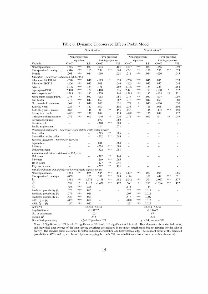
Table 6: Dynamic Unobserved Effects Probit ModelSpecification 1 Specification 2

Nonemployment Firm-provided Nonemployment Firm-providedequation training equation equation training equation

Variable Coeff. S.E. Coeff. S.E. Coeff. S.E. Coeff. S.E.Nonemploymentt−1 1.715 *** .033 -.093 .101 1.717 *** .033 -.156 .099Firm-provided trainingt−1 -.546 *** .115 .738 *** .060 -.281 ** .111 .756 *** .059Female .205 *** .044 -.010 .051 .211 *** .044 -.056 .045Education - Reference: Education ISCED 0-2Education ISCED 5-7 -.270 *** .046 -.113 * .059 -.266 *** .046 .086 .053Education ISCD 3 -.206 *** .035 .001 .046 -.205 *** .035 .057 .044Age/10 -1.732 *** .154 .171 .259 -1.759 *** .154 .243 .254Age squared/1000 2.408 *** .177 -.418 .336 2.441 *** .177 -.570 * .332Work experience/10 1.285 *** .185 -.279 .340 1.285 *** .185 -.635 ** .321Work exper. squared/1000 .073 * .037 -.013 .061 .077 ** .037 -.007 .059Bad health .218 *** .042 .062 .062 .218 *** .042 .050 .060No. household members .069 * .040 .006 .051 .071 * .040 -.030 .050Kids<12 years .227 * .127 .012 .108 .234 * .126 .001 .104Kids<12 years∗Female .165 .146 -.311 ** .155 .156 .146 -.433 *** .150Living in a couple -.493 *** .136 .049 .139 -.498 *** .136 .098 .137ln(household net income) .072 *** .015 -.040 ** .020 .071 *** .015 -.041 ** .019Permanent contract – – .072 .062 – – – –Part-time job – – -.310 *** .083 – – – –Public employment – – .114 .071 – – – –Occupation indicators – Reference: High-skilled white collar workerBlue collar – – -.215 ** .085 – – – –Low-skilled white collar – – -.202 *** .063 – – – –Sectoral indicators – Reference: ServicesAgriculture – – .041 .384 – – – –Industry – – -.224 *** .086 – – – –Unknown sector – – -.322 *** .081 – – – –Job tenure indicators – Reference: 0-4 yearsUnknown – – -.312 ** .144 – – – –5-9 years – – -.269 *** .065 – – – –10-14 years – – -.227 ** .091 – – – –15 years or more – – -.267 ** .121 – – – –Initial conditions and unobserved heterogeneity support pointsNonemployment0 1.384 *** .075 .505 *** .115 1.407 *** .077 .004 .085Firm-provided training0 -.059 .105 .357 *** .069 -.144 .102 .449 *** .071v̂1j 1.998 *** 6.571 -2.199 *** .482 2.042 *** .304 -2.067 *** .477v̂2j .539 * 1.812 -1.426 *** .497 .560 * .297 -1.284 *** .472ρ̂v -.665 *** .208 .114 .144Predicted probability p̂1 .326 *** .015 – – .325 *** 0.017 – –Predicted probability p̂2 .274 *** .021 – – .297 *** 0.022 – –Predicted probability p̂3 .520 *** .009 – – .518 *** 0.009 – –APE: p̂2 − p̂1 -.052 *** .012 – – -.028 *** 0.012 – –APE: p̂2 − p̂3 -.247 *** .025 – – -.221 *** 0.025 – –NT (N ) 33,348 (7,275) 33,348 (7,275)Log-likelihood -11,812.7 -11,946.7No. of parameters 103 67Pseudo-R2 .542 .536Test of independent eq. χ2

1=5.32 p-value=.021 χ21=.94 p-value=.332

Notes: * Significant at 10% level; ** significant at 5% level; *** significant at 1% level. Time dummies, form size indicators,and individual time average of the time-varying covariates are included in the model specification but not reported for the sake ofbrevity. The standars errors are robust to within-individual correlation and heteroskedasticity. The standard errors of the predictedprobabilities, APEs, and ρu are obtained by bootstrapping the resuls 399 times (individual-cluster bootstrap with replacement).

15

Table 7: Dynamic Unobserved Effects Probit ModelSpecification 3 Specification 4

Nonemployment Firm-provided Nonemploymentequation training equation equation

Variable Coeff. S.E. Coeff. S.E. Coeff. S.E.Nonemploymentt−1 2.155 *** .035 -.254 .240 2.155 *** .035Firm-provided trainingt−1 -.311 *** .086 .925 *** .045 -.304 *** .085Female .143 *** .033 -.020 .046 .144 *** .033Education - Reference: Education ISCED 0-2Education ISCED 5-7 -.199 *** .037 -.087 * .048 -.199 *** .038Education ISCD 3 -.143 *** .029 .016 .039 -.143 *** .029Age/10 -1.299 *** .135 .292 .224 -1.304 *** .135Age squared/1000 1.827 *** .161 -.592 ** .290 1.832 *** .160Work experience/10 1.300 *** .205 -.372 .276 1.296 *** .205Work exper. squared/1000 -.048 .031 -.016 .051 -.048 .031Bad health .182 *** .041 .050 .058 .181 *** .042No. household members .051 .035 .001 .045 .050 .035Kids<12 years .171 ** .083 .000 .095 .173 ** .084Kids<12 years∗Female .123 .111 -.309 ** .137 .120 .111Living in a couple -.398 *** .101 .080 .111 -.398 *** .101ln(household net income) .064 *** .015 -.038 ** .017 .064 *** .015Permanent contract – – .109 .071 – –Part-time job – – -.275 *** .077 – –Public employment – – .120 * .070 – –Occupation indicators – Reference: High-skilled white collar workerBlue collar – – -.190 ** .074 – –Low-skilled white collar – – -.180 *** .065 – –Sectoral indicators – Reference: ServicesAgriculture – – .070 .320 – –Industry – – -.188 ** .087 – –Unknown sector – – -.289 *** .078 – –Job tenure indicators – Reference: 0-4 yearsUnknown – – -.223 * .134 – –5-9 years – – -.244 *** .058 – –10-14 years – – -.187 ** .084 – –15 years or more – – -.205 * .112 – –Constant .597 ** .266 -2.048 *** .407 .607 ** .266Initial conditions and unobserved heterogeneity correlationNonemployment0 .560 *** .036 .140 * .074 .559 *** .036Firm-provided training0 -.097 .084 .248 *** .053 -.096 .084ρ̂v -.230 .235 – –Predicted probability p̂1 .260 *** . – – .260 *** .021Predicted probability p̂2 .221 *** . – – .221 *** .026Predicted probability p̂3 .603 *** . – – .604 *** .016APE: p̂2 − p̂1 -.040 *** . – – -.039 *** .011APE: p̂2 − p̂3 -.383 *** . – – -.383 *** .040NT (N ) 33,348 (7,275) 33,348 (7,275)Log-likelihood -11,937.8 -7,441.8No. of parameters 99 31Pseudo-R2 .537 .639Test of independent eq. χ2

1=.36 p-value=.843 –Notes: * Significant at 10% level; ** significant at 5% level; *** significant at 1% level. Time dummies,firm size indicators, and individual time average of the time-varying covariates are included in the modelspecification but not reported for the sake of brevity. The standars errors are robust to within-individualcorrelation and heteroskedasticity. The standard errors of the predicted probabilities and APEs are ob-tained by bootstrapping the resuls 399 times (individual-cluster bootstrap with replacement).

16

distribution. The state dependence of nonemployment is overestimated: the predictedprobability p̂3 and the estimated coefficient of the lagged nonemployment indicator areindeed much larger than those in specification 1. The APE of employment with traininginstead of employment without training is equal to -0.040 and, therefore, it is slightlyoverestimated by the failure in capturing cross-equation correlation.

Looking at the impact of exogenous variables on the nonemployment probability,women are less likely to be at work. The profile of the age and nonemployment prob-ability has an inverted U-shape while, ceteris paribus, the probability of being out of theworkforce increases with potential work experience. Higher educated people and thoseliving in a couple are more likely to be at work. Those with health problems or highhousehold income are less likely to be employed.

With regard to the firm-provided training equation, there is evidence of state depen-dence: people getting firm-provided training at t − 1 are more likely to receive firm-provided training at t. It is interesting to note that people not employed at t − 1 are aslikely to receive training at t as those who were at work without training at t− 1. Highereducated worker are less likely to receive training, but the coefficient is barely signifi-cant. There is therefore some evidence that education and firm-provided training are notcomplementary assets, in contrast to the findings in Blundell et al. (1999) for the US andthe UK. The training probability is lower for women with young kids and increasing withthe household net income, probably due to less attachment to the labour market and/ormore family commitment. Part-time workers are less likely to get firm-provided training.High skilled white collar workers are more likely to get training, suggesting that tasksand human capital formation are complementary assets. Finally, firm-provided trainingis more present in the services sector, among public employees, and among newly hiredworkers.10

4.2 Retaining Older Workers

The workforce is ageing in many industrialized countries. The ageing of the workforcemight be caused, in addition to demographic trends, also by the fading out of early retire-ment programs and by changes in the pension system like changes in the earliest possibleor mandatory retirement age. In the 1980s and in the first half of the 1990s, the Nether-lands had one of the lowest employment rates of elderly among the European countries.For example, in 1992 the Dutch employment rate of persons aged 55 to 64 was 28.7%

10Firm size indicators are included in the specification of the training equation (and not reported in Tables6 and 7) but they are not significantly different from zero.

17

against an European average of 39.1%.11 Given the economic stagnation in that period,the low employment rates of older workers were not seen as a major problem, whereas thehigh youth unemployment was thought of being problematic. Early retirement programswere promoted with the aim of giving a contribution to the employment of new entrants inthe labour market. However, with the ageing of the population and the resulting pressureson the pension system, the Dutch early retirement system was no longer sustainable. Aseries of policy reforms were introduced with the aim of reducing the generosity of theearly retirement schemes and creating incentives for postponing retirement. Hence, theresponse to population ageing was based on increasing labour supply and delaying retire-ment.12 By 2009, the employment rate of older workers had increased to 52.6%, largerthan the European average but still lower than the OECD average.

Given the ageing of the workforce, the labour market position of older workers iscause for increasing concern. If employed, their position is usually fine as they are notvery likely to be dismissed. As a matter of fact, older workers are well-protected byseniority rules and employment protection legislation. Nevertheless, if older workers losetheir job, they find it very hard to find a new one. Gielen and van Ours (2006) show thatcyclical adjustments of the workforce in the Netherlands occur partly through fluctuationsin separations for older workers. These separations are likely to be a one-way street outof the labour force into long-term unemployment.13 Employers are indeed reluctant tohire an older worker because of the pay-productivity gap and because of the possibleobsolescence of general human capital. As training can refresh general human capital,avoid its obsolescence, and increase workers’ productivity, it can be a channel throughwhich retirement can be postponed and employability of the older workers increased.

In this Section, we focus on the effect of firm-provided training on employabilityby allowing this effect to be heterogeneous across three age categories: 26–35, 36–49,and 50–64. The corresponding indicator variables are interacted with the lags of thenonemployment indicator and of the firm-provided training indicator. The benchmarkmodel is augmented by these interactions and by the age indicators and re-estimated.

Table 8 reports the estimation results of the coefficients and APEs of primary interest.The coefficient of the interactions between the lag training indicator and the age categoriesare (jointly) not significantly different from zero. This means that firm-provided training

11These figures are available in the Eurostat webpage http://stats.oecd.org/Index.aspx?DataSetCode=-LFS_SEXAGE_I_R.

12Empirical studies found that the Dutch reforms had a positive effect on the labour force participationof older workers (Euwals et al., 2010).

13Gielen and van Ours (2006) suggest that training of older workers in public training programs wouldhelp them to acquire new skills and to adapt to new demands, such that these workers are more likely toretain their jobs.

18

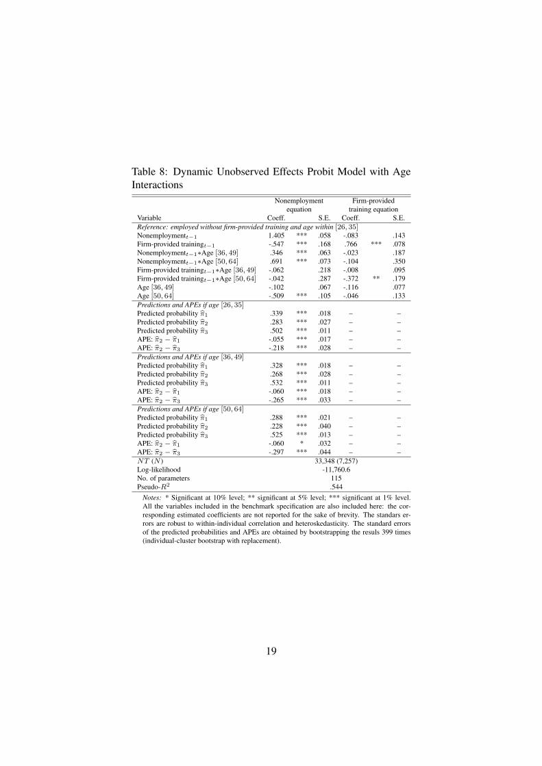
Table 8: Dynamic Unobserved Effects Probit Model with AgeInteractions

Nonemployment Firm-providedequation training equation

Variable Coeff. S.E. Coeff. S.E.Reference: employed without firm-provided training and age within [26, 35]Nonemploymentt−1 1.405 *** .058 -.083 .143Firm-provided trainingt−1 -.547 *** .168 .766 *** .078Nonemploymentt−1∗Age [36, 49] .346 *** .063 -.023 .187Nonemploymentt−1∗Age [50, 64] .691 *** .073 -.104 .350Firm-provided trainingt−1∗Age [36, 49] -.062 .218 -.008 .095Firm-provided trainingt−1∗Age [50, 64] -.042 .287 -.372 ** .179Age [36, 49] -.102 .067 -.116 .077Age [50, 64] -.509 *** .105 -.046 .133Predictions and APEs if age [26, 35]Predicted probability π̂1 .339 *** .018 – –Predicted probability π̂2 .283 *** .027 – –Predicted probability π̂3 .502 *** .011 – –APE: π̂2 − π̂1 -.055 *** .017 – –APE: π̂2 − π̂3 -.218 *** .028 – –Predictions and APEs if age [36, 49]Predicted probability π̂1 .328 *** .018 – –Predicted probability π̂2 .268 *** .028 – –Predicted probability π̂3 .532 *** .011 – –APE: π̂2 − π̂1 -.060 *** .018 – –APE: π̂2 − π̂3 -.265 *** .033 – –Predictions and APEs if age [50, 64]Predicted probability π̂1 .288 *** .021 – –Predicted probability π̂2 .228 *** .040 – –Predicted probability π̂3 .525 *** .013 – –APE: π̂2 − π̂1 -.060 * .032 – –APE: π̂2 − π̂3 -.297 *** .044 – –NT (N ) 33,348 (7,257)Log-likelihood -11,760.6No. of parameters 115Pseudo-R2 .544

Notes: * Significant at 10% level; ** significant at 5% level; *** significant at 1% level.All the variables included in the benchmark specification are also included here: the cor-responding estimated coefficients are not reported for the sake of brevity. The standars er-rors are robust to within-individual correlation and heteroskedasticity. The standard errorsof the predicted probabilities and APEs are obtained by bootstrapping the resuls 399 times(individual-cluster bootstrap with replacement).

19

is able to reduce the future probability of being out of the workforce for younger workersas well as for older workers. Note also that the interactions between lag non-employmentstatus and age categories are significantly different from zero and point out that olderworkers not employed at t− 1 are more like to be not employed at t than prime aged andyoung workers. This suggests that once older workers lose their jobs, they are less likelyto find a new one. The coefficient of the indicator for older workers is instead significantlynegative: older individuals are less likely to lose their jobs and therefore to be out of theworkforce.

The estimation of the APEs at the sample means of the other variables confirm thatfirm-provided training reduces the probability of being not employed with the same mag-nitude over age classes. An employee with a given set of observed and unobserved char-acteristics and in the age range 50–64 is 6 percentage points less likely to be out of theworkforce at t if she had been employed with training at t − 1 than if she had been em-ployed without training at t − 1. This figure is equal to that for employees in the agerange 36–49 and slightly bigger in size than that of young workers. There is evidencetherefore that firm-provided training substantially increases the employability of olderworkers as well as the employability of young workers. Firm-provided training might bean important tool to lighten the burden of population ageing on the pension system in theNetherlands.

To some extent training is endogenous to retirement institutions. In 2006 in the publicsector in the Netherlands pre-pension plans for every worker born after December 31,1949 were abolished. To receive the same pension benefits the younger cohort has topostpone retirement for about 13 months. Montizaan et al. (2010) show that this changein future pension benefits had an effect on the expected retirement age and, through this,a positive effect on workers’ training participation. We show that this is rational to dosince training leads to retaining of jobs. To retain employability of older workers age-specific subsidies to stimulate job training might be used or alternatively age-specificlayoff taxes may be introduced.14 The first type of policy would it make it more attractivefor employers to train older workers thus increasing the likelihood that they retain theiremployment. The second type of policy would make it more expensive for employersto fire older workers thus making it more attractive to train these workers and therebyincreasing the likelihood that they retain their employability.

14Schnalzenberger and Winter-Ebmer (2009) show that an age-specific firing tax affected the labourmarket position of older workers in Austria. Employers had to pay a tax of up to 170% of the gross monthlyincome when they gave notice to a worker age 50 or more. This tax caused a substantial reduction in layoffsfor older workers.

20

4.3 Further Robustness Checks

We perform two further sensitivity analyses to assess whether our estimates are robustto misspecification: i) due to omitting information about individuals who might haveattended vocational training courses not provided by the firm; ii) of the dynamics.

With regard to the former, the problem might arise as an omitted time-varying variableindicating whether the employee has undertaken training courses not provided by the firmis very likely to be correlated to the participation to a firm-provided training and, at thesame time, to the future employment status. To asses whether this might be a problem,we build an indicator variable qit equal to 1 if employee i attended vocational educationcourses which were not paid or organized by the firm since the beginning of the previousyear and 0 otherwise.15 The incidence of training not provided by the firm is equal to3.5% among the employees of our sample. Firstly, we include the variable qit in themodel specification as an exogenous variable and then as a predetermined variable (weakexogenous). In both cases, we find estimation results of the quantities of interest that arevery much in line with those of the benchmark model. Secondly, we jointly model theprocess determining training not provided by the firm and the other two equations of thebenchmark model, yielding the following simultanous three-equation model

yit = 1[yit−1δ1+wit−1γ1+qit−1λ1+x′itβ1+x̄′iα1+yi0θ1+wi0ψ1+qi0ϕ1+v1i+u1it>0]

wit = 1[yit−1δ2+wit−1γ2+qit−1λ2+z′itβ2+z̄′iα2+yi0θ2+wi0ψ2+qi0ϕ2+v2i+u2it>0] if yit=0

qit = 1[yit−1δ3+wit−1γ3+qit−1λ3+z′itβ3+z̄′iα3+yi0θ3+wi0ψ3+qi0ϕ3+κv2i+u3it>0] if yit=0,

where κ is the loading factor determining, together with v2i, the points of support of theequation of training not provided by firms. The loading factor is used to simplify thespecification of the unobserved heterogeneity distribution and reduce the computationaldifficulty in estimating the model. The likelihood function of the benchmark model canbe trivially extended to the three-equation case.

Table 9 reports the estimation results of the three-equation model. All the estimatesof the nonemployment equation and of the firm-provided equation are in line with thoseof the benchmark model reported in Table 6. Looking at the equation for training not pro-vided by the firm, it is noted that the past employment status and the past training matter:people who were nonemployed in the past are more likely to train in the future than thosewho were employed without any form of training. This type of “catch-up” response is inline with the empirical evidence in Mroz and Savage (2006), who found that recent unem-

15The indicator for vocational training not provided by the firm is built on the basis of variables PT001,PT008, and PT017 of the ECHP data.

21

Table 9: Dynamic Unobserved Effects Probit Model with 3 SimultaneousEquations

Nonemployment Firm-provided Other vocationalequation training equation training equation

Variable Coeff. S.E. Coeff. S.E. Coeff. S.E.Nonemploymentt−1 1.725 *** .034 -.065 .102 .196 ** .095Firm-provided trainingt−1 -.479 *** .116 .779 *** .060 .201 *** .076Other vocational trainingt−1 .244 *** .093 .096 .089 1.386 *** .061Female .208 *** .044 -.009 .050 .044 .056Education - Reference: Education ISCED 0-2Education ISCED 5-7 -.269 *** .046 -.102 * .058 -.027 .062Education ISCD 3 -.206 *** .035 .008 .045 -.023 .049Age/10 -1.748 *** .155 .395 .252 -.271 .187Age squared/1000 2.431 *** .179 -.697 ** .326 .194 .247Work experience/10 1.290 *** .186 -.350 .343 .156 .400Work exper. squared/1000 .073 * .038 -.003 .061 -.006 .075Bad health .218 *** .042 .060 .062 -.130 .080No. household members .072 * .040 .003 .052 -.106 .067Kids<12 years .229 * .128 .012 .110 .160 .170Kids<12 years∗Female .165 .147 -.315 ** .156 -.126 .223Living in a couple -.490 *** .138 .055 .140 .051 .146ln(household net income) .071 *** .015 -.039 ** .020 -.001 .023Permanent contract – – .083 .062 -.103 .079Part-time job – – -.298 *** .083 .245 *** .085Public employment – – .116 .072 -.148 .092Occupation indicators – Reference: High-skilled white collar workerBlue collar – – -.205 ** .086 -.253 ** .106Low-skilled white collar – – -.193 *** .064 .040 .076Sectoral indicators – Reference: ServicesAgriculture – – .050 .381 .609 ** .305Industry – – -.218 ** .086 -.030 .117Unknown sector – – -.321 *** .082 -.152 .105Job tenure indicators – Reference: 0-4 yearsUnknown – – -.289 ** .144 -.009 .1475-9 years – – -.259 *** .066 .077 .08610-14 years – – -.213 ** .092 .182 .14415 years or more – – -.245 ** .122 .230 .195Initial conditions and unobserved heterogeneity support pointsNonemployment0 1.389 *** .077 .417 *** .111 .119 .086Firm-provided training0 -.083 .107 .348 *** .067 .138 * .083Other vocational training0 .004 ** .104 .166 ** .081 .363 *** .069v̂1j 2.005 *** .307 -2.552 *** .475 – –v̂2j .540 * .300 -1.803 *** .509 – –ρ̂v -.528 * .293κ̂ .314 ** .130Predicted probability π̂1 .324 *** .015 – – – –Predicted probability π̂2 .279 *** .022 – – – –Predicted probability π̂3 .520 *** .009 – – – –APE: π̂2 − π̂1 -.045 *** .015 – – – –APE: π̂2 − π̂3 -.241 *** .025 – – – –NT (N ) 33,348 (7,275)Log-likelihood -14,535.4No. of parameters 176Pseudo-R2 .501Test of independent eq. χ2

1=224.98 p-value=.000Notes: * Significant at 10% level; ** significant at 5% level; *** significant at 1% level. Time dummies,firm size indicators, and individual time average of the time-varying covariates are included in the modelspecification but not reported for the sake of brevity. The standars errors are robust to within-individualcorrelation and heteroskedasticity. The standard errors of the predicted probabilities and APEs are obtainedby bootstrapping the resuls 239 times (individual-cluster bootstrap with replacement).

22

ployment spells has a significant positive effect on whether a young man trains today inthe US. As pointed out by Mroz and Savage (2006), the “catch-up” response is predictedby the economic theory: people with a recent nonemployment spell enter the current pe-riod with a lower stock of human capital than otherwise identical individuals. When theyre-enter the workforce, they dynamically re-optimize their investments in human capitaland their new optimal time-path of human capital investments might lie above the one ofotherwise identical individuals who did not suffer the employment shock and the loss ofhuman capital.

Table 10: Dynamic Unobserved Effects Probit Modelwith Lag of Order Two

Nonemployment Firm-providedequation training equation

Variable Coeff. S.E. Coeff. S.E.Nonemploymentt−1 1.884 *** .036 -.114 .126Nonemploymentt−2 .769 *** .042 .154 .108Firm-provided trainingt−1 -.466 *** .115 .760 *** .060Predictions and APEs if the individual was employed at t− 2Predicted probability π̂1 .232 *** .030 – –Predicted probability π̂2 .172 *** .035 – –Predicted probability π̂3 .533 *** .015 – –APE: π̂2 − π̂1 -.060 *** .016 – –APE: π̂2 − π̂3 -.361 *** .046 – –Predictions and APEs if the individual was not employed at t− 2Predicted probability π̂1 .343 *** .019 – –Predicted probability π̂2 .274 *** .031 – –Predicted probability π̂3 .688 *** .029 – –APE: π̂2 − π̂1 -.068 *** .019 – –APE: π̂2 − π̂3 -.414 *** .056 – –NT (N ) 33,348 (7,275)Log-likelihood -8,999.0No. of parameters 103Pseudo-R2 .550

Notes: * Significant at 10% level; ** significant at 5% level; *** significantat 1% level. All the variables included in the benchmark specification are alsoincluded here: the corresponding estimated coefficients are not reported for thesake of brevity. The standars errors are robust to within-individual correlationand heteroskedasticity. The standard errors of the predicted probabilities andAPEs are obtained by bootstrapping the resuls 399 times (individual-clusterbootstrap with replacement).

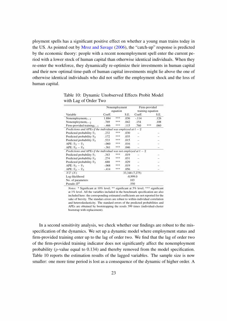
In a second sensitivity analysis, we check whether our findings are robust to the mis-specification of the dynamics. We set up a dynamic model where employment status andfirm-provided training enter up to the lag of order two. We find that the lag of order twoof the firm-provided training indicator does not significantly affect the nonemploymentprobability (p-value equal to 0.134) and thereby removed from the model specification.Table 10 reports the estimation results of the lagged variables. The sample size is nowsmaller: one more time period is lost as a consequence of the dynamic of higher order. A

23

nonemployment event at t− 2 reinforces the positive effect of a nonemployment event att − 1 on the probability of being out of the workforce at t. The estimated coefficient oflagged training is qualitatively in line with the one of the benchmark model. We estimatedthe APEs by conditioning on the nonemployment status at t − 2. In case of employmentat t − 2, the APE of working with training at t − 1 rather than working without trainingat t− 1 is of -6 percentage points in the probability of being nonemployed (-26%). If notat work at t − 2, the APE is equal to -6.8 percentage points (-20%). This suggests thatthe estimated APE π̂2 − π̂1 of our benchmark model is not sensitive to the dynamic spec-ification and, if any, it suffers from an upward bias. Note however that when we take themodel with a dynamic of higher order, we lose observations and we restrict the analysisto individuals that are in the panel for at least four consecutive waves. This makes the as-sumption of no attrition less likely to hold. We therefore prefer to stick to the specificationwith a dynamic of order one.

5 Conclusions

This paper studies the relationship between on-the-job training and employability in theNetherlands. In our analysis we disentangle the true effect of training from the spuri-ous effect that might be induced by self-selection of non-random individuals into train-ing participation. We find that firm-provided training significantly improves employmentprospects. For prime age workers who generally have a strong labour market position, inthe sense that after job loss they find a new job quite easily, this relationship may be oflimited interest. However, we also investigate whether for older workers training leadsto higher employability. We find that older workers who receive on-the-job training aremore likely to keep employment.

In many countries the labour market position of older workers is cause for concern.Older workers’ job separations are often a one-way street out of the labour force andinto long-term unemployment. This is a reason for concern since demographic trends arecausing an ageing of the workforce. Therefore, improving the employment position ofolder workers is very important from a policy point of view. Our research findings suggestthat on-the-job training may be an important instrument to achieve this goal. Our researchdoes not provide direct evidence on how to stimulate on-the-job training. Nevertheless wesuggest that, in order to retain employability of older workers, age-specific subsidies tostimulate job training might be used or, alternatively, age-specific layoff taxes may beintroduced. The first type of policy would make it more attractive for employers to trainolder workers, thus increasing the likelihood that they retain their employability. The

24

second type of policy would make it more expensive for employers to fire older workers,thus making it more attractive to train these workers and thereby increasing the likelihoodthat their employment prospects improve.

ReferencesAlessie R, Hochguertel S, van Soest A. 2004. Ownership of stocks and mutual funds: A panel data analysis.

Review of Economics and Statistics 86: 783–796.

Andrén T, Andrén D. 2006. Assessing the employment effects of vocational training using a one-factormodel. Applied Economics 38: 2469–2486.

Barrett A, O’Connell P. 2001. Does training generally work? The returns to in-company training. Industrialand Labor Relations Review 54: 647–662.

Bartel A. 1994. Productivity gains from the implementation of employee training programs. IndustrialRelations 33: 411–425.

Bartel A. 1995. Training, wage growth, and job performance: Evidence from a company database. Journalof Labor Economics 13: 401–425.

Bassi L. 1984. Estimating the effect of training programs with non-random selection. Review of Economicsand Statistics 66: 36–43.

Blundell R, Dearden L, Meghir C, Sianesi B. 1999. Human capital investments: The returns from educationand training to the individual, the firm, and the economy. Fiscal Studies 20: 1–23.

Bonnal L, Fougère D, Sérandon A. 1997. Evaluating the impact of French employment policies on individ-ual labour market histories. Review of Economic Studies 64: 683–713.

Boone J, van Ours J. 2009. Bringing unemployed back to work: Effective active labor market policies. DeEconomist 157: 293–313.

Chamberlain G. 1984. Panel data. In Grichiles Z, Intriligator M (eds.) Handbook of Econometrics, chap-ter 22. Amsterdam: North Holland, 1248–1318.

Conti G. 2005. Training, productivity and wages in Italy. Labour Economics 12: 557–576.

Crépon B, Ferracci M, Fougère D. 2007. Training the unemployed in France: How does it affect unem-ployment duration and recurrence? IZA Discussion Paper No. 3215, Bonn.

Dearden L, Reed H, Van Reenen J. 2006. The impact of training on productivity and wages: Evidence fromBritish panel data. Oxford Bulletin of Economics and Statistics 68: 397–421.

Euwals R, van Vuuren D, Wolthoff R. 2010. Early retirement behaviour in the Netherlands: Evidence froma policy reform. De Economist 158: 209–236.

Gerfin M, Lechner M. 2002. A microeconometric evaluation of the active labour market policy in Switzer-land. Economic Jounal 112: 854–893.

25

Gielen A, van Ours J. 2006. Age-specific cyclical effects in job reallocation and labor mobility. LabourEconomics 13: 493–504.

Gritz R. 1993. The impact of training on the frequency and duration of employment. Journal of Economet-rics 57: 21–51.

Ham J, LaLonde R. 1996. The effect of sample selection and initial conditions in duration models: Evidencefrom experimental data on training. Econometrica 64: 175–205.

Heckman J. 1981. The incidental parameters problem and the problem of initial conditions in estimating adiscrete time-discrete data stochastic process. In Manski C, McFadden D (eds.) Structural Analysis ofDiscrete Data with Econometric Applications, chapter 4. Cambridge: MIT Press, 179–195.

Heckman J, RJ L, JA S. 1999. The economics and econometrics of active labor market programs. In OC A,D C (eds.) Handbook of Labor Economics, volume 3A, chapter 31. Amsterdam: Elsevier, 1865–2097.

Heckman J, Singer B. 1984. A method for minimizing the impact of distributional assumptions in econo-metric models for duration data. Econometrica 52: 271–320.

Hyslop D. 1999. State dependence, serial correlation and heterogeneity in intertemporal labor force partic-ipation of married women. Econometrica 67: 1255–1294.

Jones M, Jones R, Latreille P, Sloane P. 2009. Training, job satisfaction, and workplace performance inBritain: Evidence from WERS 2004. Labour 23: 139–175.

Kluve J. 2010. The effectiveness of European active labour market programmes. Labour Economics 17:904–918.

Lalive R, van Ours J, Zweimüller F. 2008. The impact of active labour market programmes on the durationof unemployment in Switzerland. Economic Journal 118: 235–257.

Lechner M, Miquel R, Wunsh C. 2008. The curse and blessing of training the unemployed in a changingeconomy: The case of East Germany after unification. German Economic Review 8: 468–509.

Montizaan R, Corvers F, Grip AD. 2010. The effects of pension rights and retirement age on trainingparticipation: evidence from a natural experiment. Labour Economics 17: 240–247.

Mroz T, Savage T. 2006. The long-term effects of youth unemployment. Journal of Human Resources 41:259–293.

Mundlak Y. 1978. On the pooling of time series and cross section data. Econometrica 46: 69–85.

OECD. 2010. Employment Outlook. Paris.

Pavlopoulos D, Muffels R, Vermunt J. 2009. Training and low-pay mobility: The case of the UK and theNetherlands. Labour 23: 37–59.

Picchio M. 2008. Temporary contracts and transitions to stable jobs in Italy. Labour 22: 147–174.

Picchio M, van Ours J. 2011. Market imperfections and firm-sponsored training. Labour Economics 18:forthcoming.

26

Ridder G. 1986. An event history approach to the evaluation of training, recruitment and employmentprogrammes. Journal of Applied Econometrics 1: 109–126.

Sanders J, de Grip A. 2004. Training, task flexibility and the employability of low-skilled workers. Inter-national Journal of Manpower 25: 73–89.

Schnalzenberger M, Winter-Ebmer R. 2009. Layoff tax and employment of the elderly. Labour Economics16: 618–624.

Sianesi B. 2008. Differential effects of active labour market programs for the unemployed. Labour Eco-nomics 15: 370–399.

Stewart M. 2007. The interrelated dynamics of unemployment and low-wage employment. Journal ofApplied Econometrics 22: 511–531.

van den Berg G, Lindeboom M. 1998. Attrition in panel survey data and the estimation of multi-state labormarket models. Journal of Human Resources 33: 458–478.

van den Berg G, Ridder G. 1994. Attrition in longitudinal panel data and the empirical analysis of dynamiclabour market behaviour. Journal of Applied Econometrics 9: 421–435.

Wooldridge J. 2005. Simple solutions to the initial conditions problem in dynamic, nonlinear panel datamodels with unobserved heterogeneity. Journal of Applied Econometrics 20: 39–54.

27