review of introductory control theory - phoneoximeter · review of introductory control theory ......
TRANSCRIPT

EECE 460 Winter 2007 Guy Dumont 1
Review of Introductory Control Theory
Guy Dumont

EECE 460 Winter 2007 Guy Dumont 2
Review
Properties of Feedback From open loop to closed loop Important transfer functions Robustness and performance
Stability Routh Hurwitz Root locus Nyquist and Bode diagrams
Basic controllers Lead/lag compensators PID control
State space methods State space representation Controllability/observability State feedback, pole placement

EECE 460 Winter 2007 Guy Dumont 3
High Gain Feedback and Inversion
+
-
R(s) Y(s)U(s)H(s) G(s)
G(s)
Open-loopcontroller
( ) ( ) ( ) ( ) ( ) ( )
( ) ( )
( ) 1 ( ) ( )
Note that for ( ) 1, then
( ) ( ) 1
( ) ( ) ( ) ( )
U s H s R s H s G s U s
U s H s
R s H s G s
H s
U s H s
R s H s G s G s
= !
=+
�
� �
High gain feedback implicitly generates the inverse of G(s)without having to actually carry the inversion!

EECE 460 Winter 2007 Guy Dumont 4
From Open Loop to Closed Loop
+
-
R(s) Y(s)U(s)H(s) G(s)
G(s)
+
-
R(s) U(s)H(s) G(s)
Y(s)
For the relationship betweenR(s) and Y(s), both areequivalent

EECE 460 Winter 2007 Guy Dumont 5
Trade-offs
Although it seems that all is needed is highgain feedback, there is a cost attached to theuse of high-gain feedback It will result in very large control actions It increases the risk of instability It increase the sensitivity to measurement noise
When choosing the feedback gain, one mustbe conscious of the trade off between thosevarious issues
This is the essence of controldesign!

EECE 460 Winter 2007 Guy Dumont 6
The Feedback Loop
Setpoint Output
Output disturbance
Measurement noise

EECE 460 Winter 2007 Guy Dumont 7
The Feedback LoopTracking error
1 is called the sensitivity function
1
is called the complementary sensitivity function1
1Note that 1
1 1
SGC
GCT
GC
GCS T
GC GC
=+
=+
+ = + =+ +

EECE 460 Winter 2007 Guy Dumont 8
The Feedback Loop

EECE 460 Winter 2007 Guy Dumont 9
Four Important Transfer Functions
Input disturbance Output disturbance
Reference signal
Simple Feedback Control Loop

EECE 460 Winter 2007 Guy Dumont 10
Four Important Transfer Functions
The following four transfer functionsplay an important role in control design
1( ) ( ) ( ) ( )
1 1 1
( ) ( ) ( ) ( )1 1 1
GC GY s R s W s D s
GC GC GC
C C GCU s R s W s D s
GC GC GC
= + ++ + +
= ! !+ + +
Control sensitivity
Input sensitivity Sensitivity Complementary sensitivity

EECE 460 Winter 2007 Guy Dumont 11
RobustnessSensitivity of the closed-loop transfer function T to variationsin the process parameters:
2
2
2
2
2
We want to relate dT/T to dG/G
With we can write1
1 (1 )
(1 )
(1 )
(1 )
GCT
GC
dT C GC
dG GC GC
C GC GC
GC
C
GC
=+
= !+ +
+ !=
+
=+

EECE 460 Winter 2007 Guy Dumont 12
Robustness
2
2
(1 )
(1 )
1
1 1
1
1
dT C
dG GC
CdT dG
GC
GC dG
GC GC G
dT dG
T GC G
dT dGS
T G
=+
=+
=+ +
=+
=
EECE 460 Winter 2007 Guy Dumont 13
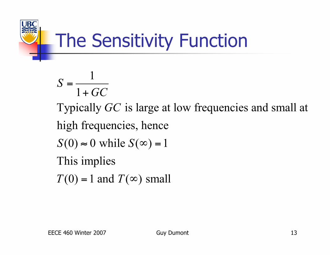
The Sensitivity Function
1
1
Typically is large at low frequencies and small at
high frequencies, hence
(0) 0 while ( ) 1
This implies
(0) 1 and ( ) small
SGC
GC
S S
T T
=+
! " =
= "

EECE 460 Winter 2007 Guy Dumont 14
Specifications
Reduce sensitivity and disturbances at lowfrequencies
Close to perfect setpoint tracking at lowfrequencies
At high frequencies, when S=1 the systemhas the same sensitivity and disturbancerejection properties as the open-loop plant
Typically S can be decreased in a frequencyrange at the cost of an increase in anotherfrequency range

EECE 460 Winter 2007 Guy Dumont 15
The Bode Integral
For a stable system Bode showed that
0log | ( ) | 0S j d! !
"
=#
“The waterbed effect ”

EECE 460 Winter 2007 Guy Dumont 16
Steady-State Error
T
T
0
0
The tracking error is
1E (s)= ( )
1+GC
For a step input
1 1E (s)=
1+GC
Using the final value theorem
lim ( ) lim ( )
1 1lim
1+GC
1( )
1 (0) (0)
t s
s
R s
s
e t sE s
ss
eG C
!" !
!
=
=
" =+
We want the steady-state error to go tozero.
Hence, if G(0) is finite,we need C(0) to beinfinite, i.e. C mustcontain one integrator1/s

EECE 460 Winter 2007 Guy Dumont 17
Test Input Signals
2
2 3
( ) ( ) ( )
( ) ( ) ( )
r t A r t At r t At
A A AR s R s R s
s s s
= = =
= = =

EECE 460 Winter 2007 Guy Dumont 18
Performance of a second-order system
2
2
2 2
2
2 2
( )( ) ( ) ( )
1 ( )
( )2
1 for a step input
2
n
n n
n
n n
G s KY s R s R s
G s s ps K
R ss s
s s s
!
"! !
!
"! !
= =+ + +
=+ +
=+ +

EECE 460 Winter 2007 Guy Dumont 19
Second-Order System
Percent Overshoot 100p v
v
M f
f
!= "

EECE 460 Winter 2007 Guy Dumont 20
Second-Order System
2
2
/ 1
4With 0.02 then
1
1
v s
n
p
n
p
f T
T
M e!" !
#!$
"
$ !
% %
=
=%
= +
�
Swiftness of response: rise time and peak timeCloseness of response: overshoot and settling time

EECE 460 Winter 2007 Guy Dumont 21
Second-Order System

EECE 460 Winter 2007 Guy Dumont 22
Steady-State Error
Reduction or elimination of steady-state error is a fundamentalreason for using feedback
0
( )( ) ( )
1 ( ) ( )
with ( ) 1
1( ) ( ) ( )
1 ( )
The steady state error is then
( )lim ( ) lim
1 ( )
a
at s
G sY s R s
G s H s
H s
E s R s Y sG s
sR se t
G s!" !
=+
=
= # =+
=+

EECE 460 Winter 2007 Guy Dumont 23
Steady-State ErrorThe number of integrators in G(s) defines its type number
0
2
0 0 0
( / )Step input: lim . For to be zero, ( ) must contain
1 ( )
at least one integrator, i.e. be of at least type 1
( / )Ramp input: lim lim lim
1 ( ) ( ) ( )
For to be
ss sss
sss s s
ss
s A se e G s
G s
s A s A Ae
G s s sG s sG s
e
!
! ! !
=+
= = =+ +
3
2 2 20 0 0
zero, ( ) must contain at least two integrators, i.e. be of at least type 2
( / )Acceleration input: lim lim lim
1 ( ) ( ) ( )
For to be zero, ( ) must contain at least th
sss s s
ss
G s
s A s A Ae
G s s s G s s G s
e G s
! ! != = =
+ +
ree integrators, i.e. be of at least type 3

EECE 460 Winter 2007 Guy Dumont 24
Error Constants2
0 0 0lim ( ) lim ( ) lim ( )
Then for
Step input 1
Ramp input
Acceleration input
p v as s s
ss
p
ss
ss
K G s K sG s K s G s
Ae
K
Ae
Kv
Ae
Ka
! ! != = =
=+
=
=

EECE 460 Winter 2007 Guy Dumont 25
Performance Indices
“A performance index is a quantitativemeasure of the performance of a system andis chosen so that emphasis is given to theimportant system specifications”
When the system parameters are chosen sothe performance index reaches an extremum(typically a minimum), then it is consideredan optimal control system
To be useful, a performance index should beeasy to optimize

EECE 460 Winter 2007 Guy Dumont 26
Performance Indices
ISE
Convenient foranalytical andcomputationalreasons
2
0
Integrated square error
( )
T
ISE e t dt= !

EECE 460 Winter 2007 Guy Dumont 27
Performance Indices
0
0
2
0
| ( ) |
| ( ) |
( )
T
T
T
IAE e t dt
ITAE t e t dt
ITSE te t dt
=
=
=
!
!
!
Integrated absolute error
Integrated time-multipliedabsolute error
Integrated time-multipliedsquared error

EECE 460 Winter 2007 Guy Dumont 28
Definitions of Stability
BIBO stability: A system is said to beBIBO stable if for any bounded input, itsoutput is also bounded.
Absolute stability: Stable /Unstable Relative stability: Degree of stability
(i.e. how far from instability) A stable linear system described by a
transfer is such that all its poles havenegative real parts

EECE 460 Winter 2007 Guy Dumont 29
Routh-Hurwitz Criterion
Consider the polynomial
Routh-Hurwitz stability criterion is a test toascertain without computing the roots,whether or not all roots of a polynomial havenegative real parts.
Today, with MATLAB, roots of a polynomialare so easily calculated that the Routh-Hurwitz criterion is hardly ever used.
1 1 1 0( )n n n n
Q s a s a s a s a! !
= + + + +L

EECE 460 Winter 2007 Guy Dumont 30
Root Locus Concept
1 ( ) 0KG s+ =
The root locus is the path of the roots of the characteristicequation traced out in the s-plane as a system parameter ischanged
K

EECE 460 Winter 2007 Guy Dumont 31
Root Locus Concept
2
2
2
2 2
* 2
* 2
11 ( ) 1 0
1
1 0
( 1) ( 1) 0
( 1) 4( 1) 2 3
1 1For 0, ( ) ( 1) 2 3
2 2
1 1For 0, ( ) ( 1) | 2 3 |
2 2
(this occurs for 1 3)
sKG s K
s s
s s Ks K
s K s K
K K K K
s K K K K
s K K j K K
K
++ = + =
+ +
+ + + + =
+ + + + =
! = + " + = " "
! > = " + ± " "
! < = " + ± " "
" < <

EECE 460 Winter 2007 Guy Dumont 32
Root Locus Concept*
*
* 2
2
1 3For 0, (0)
2 2
1For 3, (3) (3 1) 2
2
For large ,
1 1( ) ( 1) 2 1 4
2 2
1 1 ( 1) ( 1) 4
2 2
1 1 ( 1) ( 1) 1,
2 2
K s j
K s
K
s K K K K
K K
K K K
= = ! ±
= = ! + = !
= ! + ± ! + !
= ! + ± ! !
" ! + ± ! = ! !
Poles of G(s) !
Zero of G(s) !
Tends to !"

EECE 460 Winter 2007 Guy Dumont 33
Root Locus Concept1 ( ) 0
( )1 0
( )
( ) ( ) 0
When 0, this collapses to ( ) 0.
Since the roots of ( ) 0 are the poles of ( ), those are the
closed-loop poles for 0.
1 ( )When is large, ( ) ( ) 0 t
( )
KG s
N sKD s
D s KN s
K D s
D s G s
K
N sK D s KN s
K D s
+ =
+ =
+ =
= =
=
=
+ = + =( )
ends to 0( )
thus the closed-loop poles tend to the roots of ( ) 0, i.e. the
open-loop zeros, and also to infinity if is strictly proper.
N s
D s
N s
N
D
=
=

EECE 460 Winter 2007 Guy Dumont 34
Fourth-Order System
4 3 21 0 1 0
12 64 128 ( 4)( 4 4 )( 4 4 )
K K
s s s s s s s j s j+ = ! + =
+ + + + + + + "

EECE 460 Winter 2007 Guy Dumont 35
Fourth-Order System

EECE 460 Winter 2007 Guy Dumont 36
Improving Transient Response
Cannot be obtainedby gain adjustment

EECE 460 Winter 2007 Guy Dumont 37
Polar Plot or Nyquist Diagram
2
2
2 4 2 2 4 2
1
2 4 2 2
1
( )( 1)
( )
( )
1( ) tan
K KG j
j j j
K jK
KG
!! !" ! ! "
! " !
! ! " ! ! "
!
! ! "
# !!"
$
= =+ $
$= $
+ +
=
+
% &= $ ' (
$) *

EECE 460 Winter 2007 Guy Dumont 38
Bode Diagram
1
1 s!+
EECE 460 Winter 2007 Guy Dumont 39
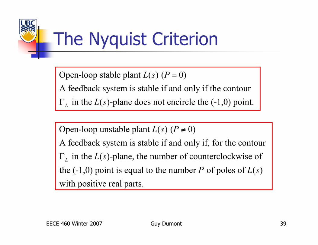
The Nyquist Criterion
Open-loop stable plant ( ) ( 0)
A feedback system is stable if and only if the contour
in the ( )-plane does not encircle the (-1,0) point.
Open-loop unstable plant ( ) ( 0)
A feedback system is s
L
L s P
L s
L s P
=
!
"
table if and only if, for the contour
in the ( )-plane, the number of counterclockwise of
the (-1,0) point is equal to the number of poles of ( )
with positive real parts.
LL s
P L s
!

EECE 460 Winter 2007 Guy Dumont 40
Relative Stability
1 2
1 2
1 2
1 2
1 2
( )( 1)( 1)
crosses the real axis at
System is marginally stable when
1, when
KGH j
j j j
Ku
u K
!! !" !"
" "
" "
" "
" "
=+ +
#=
+
+= # =
Ultimate point

EECE 460 Winter 2007 Guy Dumont 41
Gain and Phase Margins on the Bode Diagram

EECE 460 Winter 2007 Guy Dumont 42
Gain Margin
180
180
The factor by which the gain at ultimate point can be
increased to reach marginal stability
1 1
( )
Expressed in dB:
120log( ) 20log
20log ( ) dB
G
G
d L j
M dd
M L j
!
!
=
= = "
= "
Reasonable values aregain margins in the range[2 5], or in dB [6 14]dB.

EECE 460 Winter 2007 Guy Dumont 43
Phase Margin
The phase margin is , the difference between and
the phase of the loop at the crossover frequency
arg ( )
c
cM L j!
! "
#
" #
$
= +
Reasonable values are phase margins In the range [30 60] degrees

EECE 460 Winter 2007 Guy Dumont 44
Sensitivity and Nyquist Plot
( )L j!
s!
1 ( )s
L j!+
The radius r of the circle centered at -1 and tangent to L is the reciprocal of thenominal sensitivity peak
1|1 ( ) | | ( ) |s sr L j S j! ! "= + =
Critical point

EECE 460 Winter 2007 Guy Dumont 45
Lead-Lag Compensators
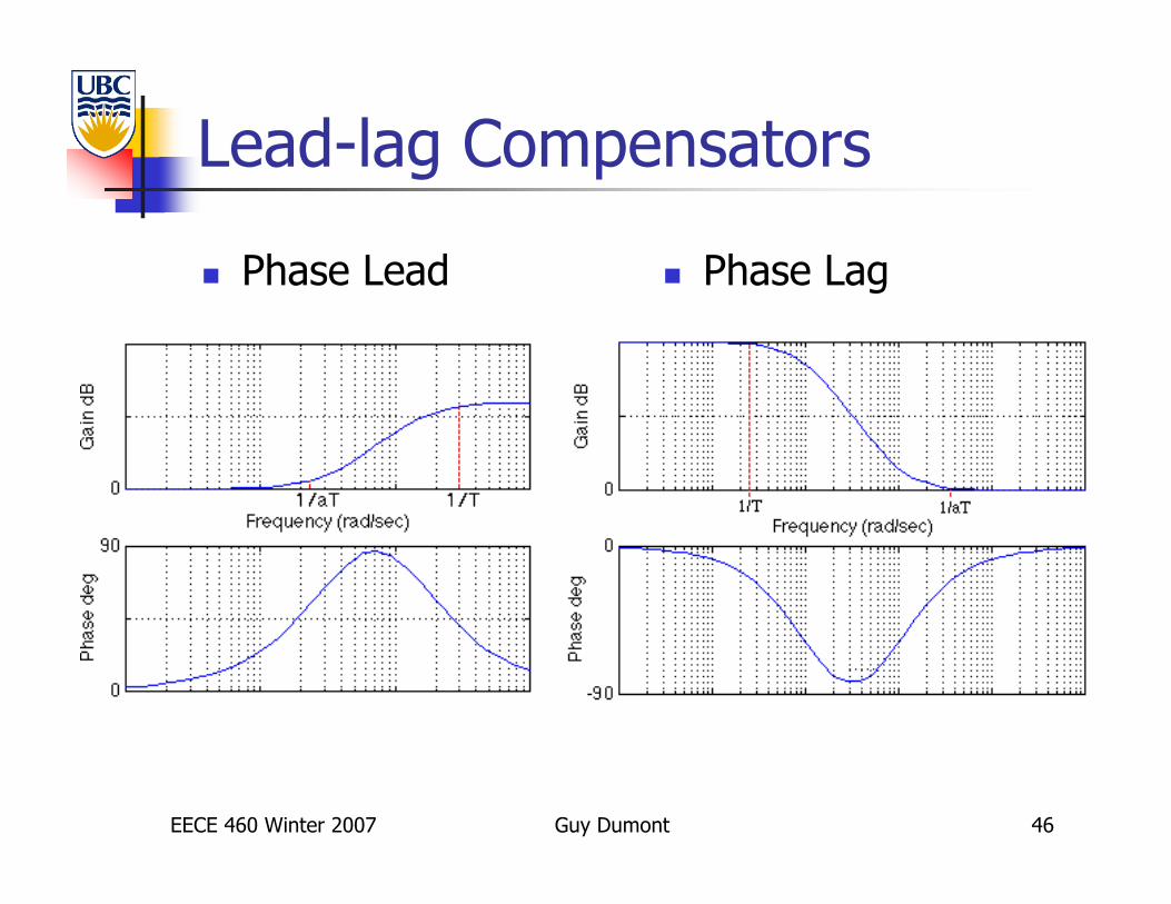
EECE 460 Winter 2007 Guy Dumont 46
Lead-lag Compensators
Phase Lead Phase Lag

EECE 460 Winter 2007 Guy Dumont 47
Systems With a Prefilter
The lead filter zero will significantlyaffect the response of the closed-loopsystem
( )( )
( ) ( ) ( ) ( )( ) ( )( )
1 ( ) ( ) 1 ( ) ( ) ( ) ( ) ( )
p c
c c
z s zG s
G s G s G s zG ss z s pT s
G s G s G s G s s p s z G s
+
+ += = =
+ + + + +

EECE 460 Winter 2007 Guy Dumont 48
Phase-Lead
Adds phase lead near crossover Increases bandwidth Increases high frequency gain Improves dynamic response Prefilter needed Requires additional amplifier gain Increases susceptibility to noise Applicable when fast response is desired Not applicable when phase decreases rapidly
near crossover frequency
EECE 460 Winter 2007 Guy Dumont 49
Phase Lag
Adds phase lag to increase error constantwhile maintaining phase margin
Decreases system bandwidth Suppresses high-frequency noise Reduces steady-state error Slows down response Applicable when error constants are specified Not applicable when no low-frequency range
exists where desired phase margin exists

EECE 460 Winter 2007 Guy Dumont 50
PID Controller
“Textbook” PID controller:
In practice:
( )
which corresponds to
( )( ) ( ) ( )
I
c P D
P I D
KG s K K s
s
de tu t K e t K e d K
dt! !
= + +
= + +"
( )1
I D
c P
D
K K sG s K
s s!= + +
+

EECE 460 Winter 2007 Guy Dumont 51
PID Controller
PI controller: Used extensively inprocess control on a broad range ofapplications due to simplicity andrelatively good performance
PD controller: Used extensively incontrolling electromechanical systems
PI controller: ( ) I
c P
KG s K
s= +
PD controller: ( )c P DG s K K s= +

EECE 460 Winter 2007 Guy Dumont 52
The State Differential Equation

EECE 460 Winter 2007 Guy Dumont 53
The State Differential Equation

EECE 460 Winter 2007 Guy Dumont 54
The State Differential Equation

EECE 460 Winter 2007 Guy Dumont 55
Transfer Function of a State Space Model
Substituting
into the output equation
( ) ( ) ( )y s Cx s Du s= +
yields

EECE 460 Winter 2007 Guy Dumont 56
Control Canonical Form1 2 1
1
1 2
0
1
1 0
...( )
...
n n
n
n n
n n
b s b s b s bG s
s a s a s a
! !
!
! !
!
+ + + +=
+ + + +
[ ]
0 1 2 1
0 1 2 1
0 1 0 ... 0 0
0 0 1 ... 0 0
0 0 0 ... 1 0
... 1
... 0
n
n n
A B
a a a a
C b b b b D
!
! !
" # " #$ % $ %$ % $ %$ % $ %= =$ % $ %$ % $ %$ % $ %! ! ! ! & '& '
= =
M M M O M M

EECE 460 Winter 2007 Guy Dumont 57
Observer Canonical Form1 2 1
1
1 2
0
1
1 0
...( )
...
n n
n
n n
n n
b s b s b s bG s
s a s a s a
! !
!
! !
!
+ + + +=
+ + + +
[ ]
0 0
1 1
2 2
1 1
0 0 0
1 0 0
0 1 0
0 0 1
0 0 ... 0 1 0
n n
a b
a b
A a B b
a b
C D
! !
!" # " #$ % $ %!$ % $ %$ % $ %= ! =$ % $ %$ % $ %$ % $ %!& ' & '
= =
L
L
L
M M O M M M
L

EECE 460 Winter 2007 Guy Dumont 58
The State Transition Matrix2 ( )
2 2
2 2
2 2
1 1( ) (0) (0) (0) (0)
2! !
1 1(0) (0) (0) (0)
2! !
1 1( ) (0)
2! !
1 1
2! !
k k
k k
k k
At k k
x t x x t x t x tk
x Ax t A x t A x tk
I At A t A t xk
e I At A t A tk
= + + + + +
= + + + + +
= + + + + +
= + + + + +
& && L L
L L
L L
L L
This series converges for all finite t. It is called the matrix exponential
( ) (0)Atx t e x=

EECE 460 Winter 2007 Guy Dumont 59
The State Transition Equation
1
t tA(t- )
0 0
( ) ( ) ( )
( ) ( ) ( )
The inverse Laplace transform gives
x(t)= e ( ) ( ) ( )
x Ax bu
sX s AX s bU s
X s sI A bU s
bu d t bu d! ! ! " ! ! !
#
= +
= +
= #
= #$ $
&
(Assumes x(0)=0)
When initial conditions are non zero:
0( ) ( ) (0) ( ) ( )
t
x t t x t bu d! ! " " "= + #$

EECE 460 Winter 2007 Guy Dumont 60
Characteristic Equation and Eigenvalues
For a transfer function G(s)=N(s)/D(s),the roots of the characteristic equation D(s)=0 are the poles of the system.
The denominator of the transfer function of a state-space representation is det(sI-A)
The characteristic equation is then det(sI-A)=0
The roots of this equation are also called the eigenvalues of the matrix A

EECE 460 Winter 2007 Guy Dumont 61
Controllability
Theorem: This system is controllable ifand only if the following controllabilitymatrix has rank n:
x Ax Bu
y Cx Du
= +
= +
&
2 1nS B AB A B A B
!" #= $ %L

EECE 460 Winter 2007 Guy Dumont 62
Observability
Theorem: This system is observable ifand only if the following observabilitymatrix has rank n:
x Ax Bu
y Cx Du
= +
= +
&
2 1T
nV C CA CA CA
!" #= $ %L

EECE 460 Winter 2007 Guy Dumont 63
State Feedback
Consider the state-space system
Let r(t) denote the reference signal Then, provided the pair [A,B] is completely
controllable, there exists a feedback of the form
such that the eigenvalues of [A-BK] can be arbitrarilyassigned
( ) ( ) ( )
( ) ( ) ( )
x t Ax t Bu t
y t Cx t Du t
= +
= +
&
1 2 3
( ) ( ) ( )
[ ]
u t r t Kx t
K k k k
= !
� L

EECE 460 Winter 2007 Guy Dumont 64
Ackermann’s Formula The state feedback gain matrix
that gives the desired characteristic equation
is given by
where
1 2 3[ ] where ( ) ( ) ( )K k k k u t r t Kx t= !� L
1
1( ) n n
nq s s s! !"
= + + +L
[ ] 10 0 1 ( )K S q A!= L
1 1
1[ ] and ( )n n n
nS B AB A B q A A A I! !" "= = + + +L L