revised methods for characterizing stream habitat … methods for characterizing stream habitat in...
TRANSCRIPT
Revised Methods for Characterizing StreamHabitat in the National Water-Quality
Assessment Program
U.S. Geological SurveyWater-Resources Investigations Report 98-4052
U.S. Department of the InteriorU.S. Geological Survey

ACKNOWLEDGMENTS
Technical Support
Thomas F. Cuffney, Ecologist, U.S. Geological Survey, Raleigh, N.C.Terry M. Short, Physical Scientist, U.S. Geological Survey, Menlo Park, Calif.Steven L. Goodbred, Biologist, U.S. Geological Survey, Sacramento, Calif.Paul L. Ringold, Ecologist, U.S. Environmental Protection Agency, Corvallis, Oreg.
Technical Reviewers
Janet S. Heiny, Hydrologist, U.S. Geological Survey, Denver, Colo.Cliff R. Hupp, Botanist, U.S. Geological Survey, Reston, Va.Robert B. Jacobson, Research Hydrologist, U.S. Geological Survey, Columbia, Mo.Peter M. Ruhl, Hydrologist, U.S. Geological Survey, Raleigh, N.C.Charles A. Peters, Supervisory Hydrologist, U.S. Geological Survey, Madison, Wis.
Editorial and Graphics
Rebecca J. Deckard, Supervisory Writer/Editor, U.S. Geological Survey, Raleigh, N.C.Kay E. Hedrick, Writer/Editor, U.S. Geological Survey, Raleigh, N.C.Jeffrey L. Corbett, Scientific Illustrator, U.S. Geological Survey, Raleigh, N.C.Michael Eberle, Technical Publications Editor, U.S. Geological Survey, Columbus, OhioBetty B. Palcsak, Technical Publications Editor, U.S. Geological Survey, Columbus, Ohio
Approving Official
Chester Zenone, Reports Improvement Advisor, U.S. Geological Survey, Reston, Va.

U.S. GEOLOGICAL SURVEY
Water-Resources Investigations Report
Revised Methods for CharacterizingStream Habitat in the National Water-Quality Assessment Program
By Faith A. Fitzpatrick, Ian R. Waite, Patricia J. D’Arconte, Michael R. Meador, Molly A. Maupin, and Martin E. Gurtz
Raleigh, North Carolina1998
98-4052

U.S. DEPARTMENT OF THE INTERIORBRUCE BABBITT, Secretary
U.S. GEOLOGICAL SURVEY
Thomas J. Casadevall, Acting Director
The use of firm, trade, and brand names in this report is for identification purposes only and doesnot constitute endorsement by the U.S. Geological Survey.
For additional information write to: Copies of this report can be purchased
U.S. Geological SurveyBranch of Information ServicesBox 25286, Federal CenterDenver, CO 80225-0286
from:
District ChiefU.S. Geological Survey3916 Sunset Ridge RoadRaleigh, NC 27607-6416
Foreword III
The mission of the U.S. Geological Survey (USGS) is to assess the quantity and quality of the earth resources of the Nation and to provide information that will assist resource managers and policymakers at Federal, State, and local levels in making sound decisions. Assessment of water-quality conditions and trends is an important part of this overall mission.
One of the greatest challenges faced by water-resources scientists is acquiring reliable information that will guide the use and protection of the Nation’s water resources. That challenge is being addressed by Federal, State, interstate, and local water-resource agencies and by many academic institutions. These organizations are collecting water-quality data for a host of purposes that include compliance with permits and water-supply standards; development of remediation plans for a specific contamination problem; operational decisions on industrial, wastewater, or water-supply facilities; and research on factors that affect water quality. An additional need for water-quality information is to provide a basis on which regional and national-level policy decisions can be based. Wise decisions must be based on sound information. As a society we need to know whether certain types of water-quality problems are isolated or ubiquitous, whether there are significant differences in conditions among regions, whether the conditions are changing over time, and why these conditions change from place to place and over time. The information can be used to help determine the efficacy of existing water-quality policies and to help analysts determine the need for, and likely consequences of, new policies.
To address these needs, the Congress appropriated funds in 1986 for the USGS to begin a pilot program in seven project areas to develop and refine the National Water-Quality Assessment (NAWQA) Program. In 1991, the USGS began full implementation of the program. The NAWQA Program builds upon an existing base of water-quality studies of the USGS, as well as those of other Federal, State, and local agencies. The objectives of the NAWQA Program are to
• Describe current water-quality conditions for a large part of the Nation’s freshwater streams, rivers, and aquifers.
• Describe how water quality is changing over time.
• Improve understanding of the primary natural and human factors that affect water-quality conditions.
This information will help support the development and evaluation of management, regulatory, and monitoring decisions by other Federal, State, and local agencies to protect, use, and enhance water resources.
The goals of the NAWQA Program are being achieved through ongoing and proposed investigations of 60 of the Nation’s most important river basins and aquifer systems, which are referred to as Study Units. These Study Units are distributed throughout the Nation and cover a diversity of hydrogeologic settings. More than two-thirds of the Nation’s freshwater use occurs within the 60 Study Units and more than two- thirds of the people served by public water-supply systems live within their boundaries.
National synthesis of data analysis, based on aggregation of comparable information obtained from the Study Units, is a major component of the program. This effort focuses on selected water-quality topics using nationally consistent information. Comparative studies will explain differences and similarities in observed water-quality conditions among study areas and will identify changes and trends and their causes. The first topics addressed by the national synthesis are pesticides, nutrients, volatile organic compounds, and aquatic biology. Discussions on these and other water-quality topics will be published in periodic summaries of the quality of the Nation’s ground and surface water as the information becomes available.
This report is an element of the comprehensive body of information developed as part of the NAWQA Program. The program depends heavily on the advice, cooperation, and information from many Federal, State, interstate, Tribal, and local agencies and the public. The assistance and suggestions of all are greatly appreciated.
Robert M. HirschChief Hydrologist
FOREWORD
CONTENTS
Foreword................................................................................................................................................................................ IIIGlossary ................................................................................................................................................................................ VIIAbstract ................................................................................................................................................................................. 1Introduction .......................................................................................................................................................................... 1Summary of revisions to original protocol ........................................................................................................................... 2Habitat-sampling design ....................................................................................................................................................... 3
Conceptual framework for characterizing stream habitat ........................................................................................... 3Relevance and application to other habitat-assessment techniques ............................................................................ 4Selection of sampling sites ......................................................................................................................................... 5Sampling strategy for fixed and synoptic sites ........................................................................................................... 5Preferred units of measure .......................................................................................................................................... 5
Basin characterization ........................................................................................................................................................... 7Background ................................................................................................................................................................. 7Description and list of basin characteristics ............................................................................................................... 10
Segment characterization ...................................................................................................................................................... 15Background ................................................................................................................................................................. 15Description and list of segment characteristics .......................................................................................................... 18
Reach characterization .......................................................................................................................................................... 21Selection of a reach ..................................................................................................................................................... 21Collection of general reach data and placement of transects ...................................................................................... 22Identification of banks and bankfull stage .................................................................................................................. 26
Empirical relations for identifying bankfull stage ............................................................................................ 28Field indicators of bankfull stage ..................................................................................................................... 28
Collection of transect data .......................................................................................................................................... 30Additional optional measurements ............................................................................................................................. 33
Surveys of channel cross sections .................................................................................................................... 34Riparian-vegetation characterization ................................................................................................................ 35Substrate characterization ................................................................................................................................. 37
Description and list of reach-scale habitat characteristics .......................................................................................... 38General reach information ................................................................................................................................ 38Transect information ......................................................................................................................................... 41
Equipment list ............................................................................................................................................................. 46Data management ................................................................................................................................................................. 46
Forms .......................................................................................................................................................................... 46Habitat data dictionary ................................................................................................................................................ 46
Data analysis ......................................................................................................................................................................... 48Data-application examples ................................................................................................................................................... 50
Willamette Basin ........................................................................................................................................................ 50Western Lake Michigan Drainages ............................................................................................................................. 52
Synoptic study .................................................................................................................................................. 52Basic fixed sites ................................................................................................................................................ 53
Summary ............................................................................................................................................................................... 54References cited .................................................................................................................................................................... 54Field forms ............................................................................................................................................................................ 60
Contents V

... 17
.... 26
...... 27
.... 31
......
.....
... 36
..... 8
...... 10
.....
.... 51
FIGURES
1. Sketches showing spatial hierarchy of basin, stream segment, stream reach, and microhabitat ...................... 42–3. Diagrammatic examples of how to:
2. Measure sinuosity .................................................................................................................................. 163. Calculate (A) Strahler stream order and (B) Shreve stream order (link) and downstream link ..........
4. Diagram of the three main geomorphic channel units....................................................................................... 225. Example of a diagrammatic stream map showing transect locations, reach boundary markers,
and other important stream characteristics ....................................................................................................... 246. Diagram of how to measure water-surface gradient with a clinometer or surveyor’s level .........................7. Diagrammatic examples of the relative position of geomorphic features, bankfull stage,
and bank angle from (A) a bend in a meandering stream, and (B) a straight reach ...................................8. Graphs showing average values for bankfull channel features in relation to drainage area
for four regions of the United States ................................................................................................................ 299–10. Diagrams showing:
9. Measurement of open canopy angle ...................................................................................................... 3010. A concave spherical densiometer with bubble level, tape, and 17 points of observation ..................
11. Field scale for identifying particle-size classes from sand to small cobble ...................................................... 3312. Sample notes for channel cross-section survey and water-surface gradient .............................................. 3413. Diagrammatic example of measurement points for cross-section profiles .................................................35
14–15. Diagrams showing:14. Point-centered quarter method used to evaluate density and dominance of bank woody vegetation15. Tables in the habitat data dictionary ...................................................................................................... 48
16. Graph showing results from canonical correspondence analysis of fish relative abundance and five environmental variables in the Willamette Basin, Oregon ........................................................................ 52
TABLES
1. Sampling strategy for habitat measurements at National Water-Quality Assessment Program basic fixed sites and synoptic sites.................................................................................................................... 6
2. Commonly measured geomorphic descriptors of drainage basins from 7.5-minute topographic maps ......3. Drainage-basin and stream-network characteristics that can be measured with Basinsoft software ..........4. Explanation of the bank stability index............................................................................................................. 325. Equipment and supplies for measuring reach and transect characteristics................................................... 476. Habitat data dictionary tables and their contents............................................................................................... 487. Results from principal components analysis of habitat data from the Willamette Basin, 1994....................
CONVERSION FACTORS
Multiply By To obtain
Length
millimeter (mm) 0.03937 inchcentimeter (cm) 0.3937 inch
meter (m) 3.281 footkilometer (km) 0.6214 mile
Area
square meter (m2) 10.76 square footsquare kilometer (km2) 0.38361 square mile
Volume per unit time (flow)
cubic meter per second (m3/s) 35.31 cubic foot per second
VI Contents

t
t,
e l e
ly
its
ts
GLOSSARY
The terms in this glossary were compiled from numerous sources. Some definitions have been modified in accordance with the usage of the National Water-Quality Assessment (NAWQA) Program and may not be the only valid definitions for these terms.
Aggradation—A long-term, persistent rise in the elevation of a streambed by deposition of sediment. Aggradation can result from a reduction of discharge with no corresponding reduction in sediment load, or an increase in sediment load with no change in discharge.
Bank—The sloping ground that borders a stream and confines the water in the natural channel when the water level, or flow, is normal. It is bordered by the flood plain and channel.
Bankfull stage—Stage at which a stream first overflows its natural banks formed by floods with 1- to 3-year recurrence intervals (Langbein and Iseri, 1960; Leopold and others, 1964).
Base flow—Sustained, low flow in a stream; ground-water discharge is the source of base flow in most streams.
Basic fixed sites—Sites on streams at which streamflow is measured and samples are collected for measurements of temperature, salinity, and suspended sediment, and analyses for major ions and metals, nutrients, and organic carbon to assess the broad-scale spatial and temporal character and transport of inorganic constituents of streamwater in relation to hydrologic conditions and environmental settings.
Canopy angle—Generally, a measure of the openness of a stream to sunlight. Specifically, the angle formed by an imaginary line from the highest structure (for example, tree, shrub, or bluff) on one bank to eye level at mid-channel to the highest structure on the other bank.
Channel—The channel includes the thalweg and streambed. Bars formed by the movement of bedload are included as part of the channel.
Channelization—Modification of a stream, typically by straightening the channel, to provide more uniform flow. Channelization is often done for flood control or for improved agricultural drainage or irrigation.
Confluence—The flowing together of two or more streams; the place where a tributary joins the main stream.
Contributing area—The area in a drainage basin that contributes runoff to a stream.
Crenulation—A “V” or “U” shaped indentation in a contour line that represents a course for flowing water (ephemeral, intermittent, or perennial stream) on a topographic map. The point forming the crenulation faces upstream.
Cross section—A line of known horizontal and vertical elevation across a stream perpendicular to the flow. Measurements are taken along this line so that geomorphological characteristics of the section are measured
with known elevation from bank to bank. Compare to transect.
Diversion—A turning aside or alteration of the natural course of flowing water, normally considered to physically leave the natural channel. In some States, this can be a consumptive use directly from another source, such as bylivestock watering. In other States, a diversion must consisof such actions as taking water through a canal, pipe, or conduit.
Drainage area—An area of land that drains water, sedimenand dissolved materials to a common outlet along a streamchannel. The area is measured in a horizontal plane and enclosed by a drainage divide.
Drainage basin—A part of the surface of the Earth that is occupied by a drainage system, which consists of a surfacstream or a body of impounded surface water, including altributary surface streams and bodies of impounded surfacwater.
Ecoregion—An area of similar climate, landform, soil, potential natural vegetation, hydrology, or other ecologicalrelevant variables.
Embeddedness—The degree to which gravel-sized and larger particles are surrounded or enclosed by finer-sized particles.
Ephemeral stream—A stream that carries water only duringperiods of rainfall or snowmelt events (Leopold and Miller,1956).
Flood—Any relatively high streamflow that overtops the natural or artificial banks of a stream.
Flood plain—The relatively level area of land bordering a stream channel and inundated during moderate to severe floods. The level of the flood plain is generally about the stage of the 1- to 3-year flood.
Geomorphic channel units—Fluvial geomorphic descriptors of channel shape and stream velocity. Pools, riffles, and runs are three types of geomorphic channel unconsidered for National Water-Quality Assessment (NAWQA) Program habitat sampling.
Habitat—In general, aquatic habitat includes all nonliving (physical) aspects of the aquatic ecosystem (Orth, 1983), although living components like aquatic macrophytes and riparian vegetation also are usually included. Measuremenof habitat are typically made over a wider geographic scalethan measurements of species distribution.
Hydrography—Surface-water drainage network.
Hypsography—Elevation contours.
Glossary VII

nt,
n
e
gh
s
n
r
1-
l)
g
the
Indicator sites—Stream sampling sites located at outlets of drainage basins with relatively homogeneous land use and physiographic conditions. Most indicator-site basins have drainage areas ranging from 52 to 520 square kilometers.
Integrator or mixed-use sites—Stream sampling sites located at outlets of drainage basins that contain multiple environmental settings. Most integrator sites are on major streams with relatively large drainage areas.
Intensive fixed sites—Basic fixed sites with increased sampling frequency during selected seasonal periods and analysis of dissolved pesticides for 1 year. Most NAWQA Study Units have one to two integrator intensive fixed sites and one to four indicator intensive fixed sites.
Intermittent stream—A stream in which, at low flow, dry reaches alternate with flowing ones along the stream length (Leopold and Miller, 1956).
Lattice elevation model—A file of terrain elevations stored in a grid format.
Perennial stream—A stream that carries some flow at all times (Leopold and Miller, 1956).
Physiography—A description of the surface features of the Earth, with an emphasis on the origin of landforms.
Pool—A small part of the reach with little velocity, commonly with water deeper than surrounding areas.
Reach—A length of stream that is chosen to represent a uniform set of physical, chemical, and biological conditions within a segment. It is the principal sampling unit for collecting physical, chemical, and biological data.
Recurrence interval—The average time period within which the size (magnitude) of a given flood will be equaled or exceeded.
Reference location—A geographic location that provides a link to habitat data collected at different spatial scales. It is often a location with known geographic coordinates, such as a gaging station or bridge crossing.
Reference site—A NAWQA sampling site selected for its relatively undisturbed conditions.
Retrospective analysis—Review and analysis of existing data in order to address NAWQA objectives, to the extent possible, and to aid in the design of NAWQA studies.
Riffle—A shallow part of the stream where water flows swiftly over completely or partially submerged obstructions to produce surface agitation.
Riparian—Pertaining to or located on the bank of a body of water, especially a stream.
Riparian zone—Area adjacent to a stream that is directly or indirectly affected by the stream. The biological community or physical features of this area are different or modified from the surrounding upland by its proximity to the river or stream.
Run—A relatively shallow part of a stream with moderate velocity and little or no surface turbulence.
Segment—A section of stream bounded by confluences or physical or chemical discontinuities, such as major waterfalls, landform features, significant changes in gradieor point-source discharges.
Sideslope gradient—The representative change in elevatioin a given horizontal distance (usually about 300 meters) perpendicular to a stream; the valley slope along a line perpendicular to the stream.
Sinuosity—The ratio of the channel length between two points on a channel to the straight-line distance between thsame two points; a measure of meandering.
Stage—The height of a water surface above an establisheddatum; same as gage height.
Stream—The general term for a body of flowing water. Generally, this term is used to describe water flowing throua natural channel as opposed to a canal.
Streamflow—A general term for water that flows through achannel.
Stream order—A ranking of the relative sizes of streams within a watershed based on the nature of their tributaries.
Study Unit—A major hydrologic system in the United Statein which NAWQA studies are focused. Study Units are geographically defined by a combination of ground- and surface-water features and generally encompass more tha4,000 square miles of land area.
Synoptic sites—Sites sampled during a short-term investigation of specific water-quality conditions during selected seasonal or hydrologic conditions to provide improved spatial resolution for critical water-quality conditions.
Terrace—An abandoned flood-plain surface. A terrace is along, narrow, level or slightly inclined surface that is contained in a valley and bounded by steeper ascending odescending slopes, and it is always higher than the flood plain. A terrace may be inundated by floods larger than theto 3-year flood.
Thalweg—The line formed by connecting points of minimum streambed elevation (deepest part of the channe(Leopold and others, 1964).
Transect—A line across a stream perpendicular to the flowand along which measurements are taken, so that morphological and flow characteristics along the line are described from bank to bank. Unlike a cross section, no attempt is made to determine known elevation points alonthe line.
Wadeable—Sections of a stream where an investigator canwade from one end of the reach to the other, even though reach may contain some pools that cannot be waded.
VIII Glossary

Revised Methods for Characterizing Stream Habitat in the National Water-Quality Assessment ProgramBy Faith A. Fitzpatrick, Ian R. Waite, Patricia J. D’Arconte, Michael R. Meador, Molly A. Maupin, and Martin E. Gurtz
of of rs,
or ).ial
ant
ABSTRACT
Stream habitat is characterized in the U.S. Geological Survey’s National Water-Quality Assessment (NAWQA) Program as part of an integrated physical, chemical, and biological assessment of the Nation's water quality. The goal of stream habitat characterization is to relate habitat to other physical, chemical, and biological factors that describe water-quality conditions. To accomplish this goal, environmental settings are described at sites selected for water-quality assessment. In addition, spatial and temporal patterns in habitat are examined at local, regional, and national scales.
This habitat protocol contains updated methods for evaluating habitat in NAWQA Study Units. Revisions are based on lessons learned after 6 years of applying the original NAWQA habitat protocol to NAWQA Study Unit ecological surveys. Similar to the original protocol, these revised methods for evaluating stream habitat are based on a spatially hierarchical framework that incorporates habitat data at basin, segment, reach, and microhabitat scales. This framework provides a basis for national consistency in collection techniques while allowing flexibility in habitat assessment within individual Study Units. Procedures are described for collecting habitat data at basin and segment scales; these procedures include use of geographic information system data bases, topographic maps, and aerial photographs. Data collected at the reach scale include channel, bank, and riparian characteristics.
INTRODUCTION
The U.S. Geological Survey’s (USGS) National Water-Quality Assessment (NAWQA) Program is designed to assess the status of and trends in the Nation’s water quality (Gilliom and others, 1995) and to develop an understanding of the major factors that affect observed water-quality conditions and trends (Hirsch and others, 1988; Leahy and others, 1990). This assessment is accomplished by collecting physical, chemical, and biological data at sites that represent major natural and human factors (for example, ecoregion, land use, stream size, hydrology, and geology) that are thought to control water quality. These data are used to provide an integrated assessment of water quality within selected environmental settings, assess trends in water quality, and investigate the influence of major natural and human factors on water quality.
Study Unit investigations in the NAWQA Program are done on a staggered time scale in approximately 59 of the largest and most significant hydrologic systems across the Nation (Gilliom and others, 1995). These investigations, which consist of 4 to 5 years of intensive assessment followed by 5 years of low-intensity assessment, consist of four main components—(1) retrospective analysis; (2) occur-rence and distribution assessment; (3) assessment long-term trends and changes; and (4) case studiessources, transport, fate, and effects (Gilliom and othe1995). Occurrence and distribution assessments aredone in a nationally consistent and uniform manner fidentification of spatial and temporal trends in waterquality at a national scale (Gilliom and others, 1995
Characterization of stream habitat is an essentcomponent of many water-quality assessment programs (Osborne and others, 1991) and an importelement in the NAWQA Program (Gurtz, 1994).
Abstract 1
Habitat assessment is critical in determining the limiting natural and human factors that affect water chemistry and aquatic biological communities. These limiting factors exist at many different spatial scales, from drainage-basin characteristics to streambed conditions within a small area of the stream. Thus, habitat assessments consist of measuring a wide range of characteristics. For example, fish-species distribution is affected by climate (Tonn, 1990), stream gradient (Sheldon, 1968), and particle size of substrate within a specific section of a stream (Hynes, 1975). Habitat assessment provides baseline information on stream conditions so that trends resulting from natural and human causes can be identified, estimated, or predicted. Habitat assessments also are done to determine the physical, chemical, and biological consequences of alterations of stream conditions, such as stream impoundment or channelization, or of changes in land use in the drainage basin. Hence data collected as part of the habitat assessment can be used to help interpret physical (for example, channel characteristics) and chemical (for example, transport of sediment-associated contaminants) properties in addition to supporting investigations of biological communities.
Many State and regional assessment programs incorporate habitat data (Osborne and others, 1991) using guidelines with a regional or single-purpose focus (for example, Bovee, 1982; Platts and others, 1983; Hamilton and Bergersen, 1984; Platts and others, 1987); however, little national uniformity in concept or methodology currently exists (Osborne and others, 1991). Because no current habitat evaluation procedures meet national objectives of the NAWQA Program, a NAWQA habitat protocol was developed (Meador, Hupp, and others, 1993).
The goal of the NAWQA stream habitat protocol (Meador, Hupp, and others, 1993) is to measure habitat characteristics that are essential in describing and interpreting water-chemistry and biological conditions in many different types of streams studied within the NAWQA Program. To accomplish this goal, various habitat characteristics are measured at different spatial scales; some characteristics are important at the national scale, whereas others might be equally important at the Study Unit or regional scale.
The original NAWQA habitat protocol (Meador, Hupp, and others, 1993) was written at the start of the NAWQA Program with the idea that the methods described in that document were to be continuously
tested and refined and new methods evaluated. After application of the protocol by approximately 37 NAWQA Study Units over 6 years, it was determined that a revision of the NAWQA protocol was necessary. This revised protocol incorporates the experiences of NAWQA Study Units under a wide range of environmental conditions and contains examples of how the habitat data were used by the Study Units while retaining the goals of the original protocol. The revised protocol also incorporates links to the NAWQA habitat data dictionary, which provides the framework for a relational data base for storing computer files of habitat data.
The purpose of this report is to provide revised procedures for characterizing stream habitat as part of the NAWQA Program. These procedures allow for appropriate habitat descriptions and standardization of measurement techniques to facilitate unbiased evaluations of habitat influences on stream conditions at local, regional, and national scales.
This report describes the methods for collecting and analyzing habitat data at three spatial scales. Data at the basin and segment scales are collected by using a geographic information system (GIS) data base, topographic maps, and aerial photographs. Data collected at the reach scale include measurements and observations of channel, bank, and riparian characteristics. Habitat characteristics from each scale that are needed for NAWQA national data aggregation are distinguished from optional characteristics that might be important for specific Study Units. Forms for recording the habitat data are presented, and guidance on data management and analysis is provided. Examples of how the data were used in two NAWQA Study Unit investigations also are included. The glossary includes brief definitions of habitat terms found throughout the report.
SUMMARY OF REVISIONS TO ORIGINAL PROTOCOL
The revised NAWQA habitat protocol contains both major and minor updates to the original protocol. The following is a general list of major additions or changes.
2 Revised Methods for Characterizing Stream Habitat in the National Water-Quality Assessment Program

ch, rk sin,
ell t d
ale ated n
,
g as
Updates or changes affecting the entire protocol:
1. Highlighted habitat measurements in bold if required for NAWQA national data aggregation.
2. Expanded discussion of the usefulness of habitat data and how the data may correlate to aquatic community and water-chemistry data.
3. Added data-analysis section that describes how habitat data can be analyzed statistically.
4. Added examples of how habitat data were used in aquatic community and water-chemistry analyses for two NAWQA Study Units.
5. Added data-management section that links habitat data with files in the NAWQA habitat data dictionary.
6. Included several habitat characteristics from the NAWQA habitat data dictionary.
7. Updated hard-copy forms for recording habitat measurements.
8. Updated protocol on collection of habitat data on the basis of the results from a survey filled out by NAWQA Study Unit biologists.
9. Added explanation for collecting habitat data at nonwadeable sites.
Updates or changes specific to reach scale:
1. Added a description for identifying bankfull stage.
2. Added step-by-step instructions for conducting a reach characterization.
3. Increased the number of transects from six transects in the center of geomorphic channel units to 11 equidistant transects and, by reducing the number of data elements collected along each transect, kept the time requirements similar.
4. Dropped the requirements for channel cross sections and point-quarter vegetation at all basic fixed sites and converted these to Study Unit options.
5. Dropped the previous terminology of "Level I" and "Level II."
HABITAT-SAMPLING DESIGN
Relations among physical, chemical, and biological components of streams are determined not
only within the context of a stream but also within the broader context of the surrounding watershed (Hynes, 1975). Therefore, to adequately examine the relations among physical, chemical, and biological attributes of streams, evaluating stream habitat must be accomplished within a systematic framework that accounts for multiple spatial scales.
Conceptual Framework for Characterizing Stream Habitat
A framework for evaluating stream habitat must be based on a conceptual understanding of how stream systems are organized in space and how they change through time (Lotspeich and Platts, 1982; Frissell and others, 1986). Among physiographic regions, or among streams within a region, different geomorphic processes control the form and development of basins and streams (Wolman and Gerson, 1978). In addition, geomorphic conditions may be different depending on the position of the stream within the hierarchy of the stream network. Therefore, researchers have recognized the importance of placing streams and stream habitats in a geographic, spatial hierarchy (Godfrey, 1977; Lotspeich and Platts, 1982; Bailey, 1983; Frissell and others, 1986).
NAWQA uses a modification of the spatially hierarchical approach proposed by Frissell and others (1986) for describing environmental settings and evaluating stream habitat. Frissell and others (1986) included five spatial systems—stream, segment, reapool/riffle, and microhabitat. The modified approachused in the NAWQA Program consists of a framewothat integrates habitat data at four spatial scales—basegment, reach, and microhabitat (fig. 1). This approach differs from the scheme proposed by Frissand others (1986) in that (1) the term "system" is noused, (2) basin is used to refer to stream system, an(3) the pool/riffle system is omitted as a separate scto be evaluated because measurements are incorporinto the reach scale. The microhabitat scale has beefound to provide insight to patterns of relations between biota and habitat at larger scales (Hawkins1985; Biggs and others, 1990). Procedures for collection of microhabitat data are described in the NAWQA protocols for the collection of invertebrate (Cuffney and others, 1993) and algal (Porter and others, 1993) samples.
Basin and segment data are collected by usinGIS, topographic maps, or aerial photographs, where
Habitat-Sampling Design 3

d A
of
res uce
er
res
ary l
al ely s
y
to
Figure 1. Spatial hierarchy of basin, stream segment, stream reach, and microhabitat (modified from Frissell and others, 1986).
Main channel(cobble bed riffle)
Main channel(woody snag pool)
Channel margin(bar)
��������������
BASIN STREAM SEGMENT STREAM REACH MICROHABITAT
reach data require site visits. The collection of a core part of the reach-scale data is based on the systematic placement of equally spaced transects; the distance between these transects depends upon stream width. This approach was adopted to maximize repeatability and precision of measurements while minimizing observer bias; it is based in part on results from a study of optimal transect spacing and sample size for fish habitat (Simonson and others, 1994b).
Relevance and Application to Other Habitat-Assessment Techniques
Within the past couple of decades, the number of systems for habitat assessment and classification has increased substantially, and new ones are continually being published. Each assessment or classification scheme differs in goals, spatial scale, quantitativeness, the effort and time required, and applicability to different-sized streams. For example, some may be specifically designed to quantify fish habitat in wadeable streams (Simonson and others, 1994a), or to qualitatively classify State or regional stream use or potential (Ball, 1982; Michigan Department of Natural Resources, 1991). Others are more focused on channel characteristics from a geomorphic perspective (Montgomery and Buffington, 1993; Rosgen, 1994). Some have been designed for national use but are qualitative, such as the habitat component of the U.S. Environmental Protection Agency’s (USEPA’s) Rapid Bioassessment Protocol (Plafkin and others, 1989),
which is currently being revised. The habitat assessment for the USEPA’s Environmental Monitoring and Assessment Program (Kaufmann anRobison, 1994) contains goals similar to the NAWQreach-scale characterization (quantitative, national scope; consideration of time; systematic placement transects) but does not include basin or segment characterization.
The NAWQA protocol balances qualitative andquantitative measures of habitat. Qualitative measuof habitat are often advantageous because they redthe amount of time needed to collect data at a site. However, qualitative measures often incorporate observer bias; thus, they may lack repeatability (Ropand Scarnecchia, 1995). Although quantitative measures may be more precise, they increase the amount of time needed to collect data. The procedudescribed in this document represent a balance of qualitative and quantitative measures judged necessto adequately ensure national consistency, minimizeobserver bias, and maximize repeatability. IndividuaNAWQA Study Units may find additional data collection useful for comparison with State or regionassessments. Many local or regional assessments ron qualitative data to generate stream habitat indicefor classification and interpretation of stream conditions. Such approaches may not be applicableeverywhere (Stauffer and Goldstein, 1997). Data collected for local purposes (for example, to link withState assessments) should be obtained concurrentlwith measurements made for nationally consistent characterizations, thereby providing an opportunity
4 Revised Methods for Characterizing Stream Habitat in the National Water-Quality Assessment Program

year n
, l at
nce ly s, rs
r
c
s.
ts,
ty e
s
t e
the
nd
compare different methods or to support qualitative indices with quantitative measurements.
Selection of Sampling Sites
Sampling sites are generally chosen to represent the set of environmental conditions deemed important to controlling water quality in the Study Unit (Gilliom and others, 1995). Sites should represent combinations of natural and human factors thought to influence collectively the physical, chemical, and biological characteristics of water quality in the Study Unit and to be of importance locally, regionally, or nationally. Two distinct types of sampling sites are established as part of the NAWQA Program—basic fixed sites and synoptic sites.
Basic fixed sites are used to characterize the spatial and temporal distribution of general water quality and constituent transport in relation to hydrologic conditions and contaminant sources (Gilliom and others, 1995). At these sites, broad suites of physical and chemical characteristics are measured, along with characteristics of fish, benthic-invertebrate, and algal assemblages. Basic fixed sites are typically at or near USGS gaging stations where continuous discharge measurements are available. Synoptic sites are typically nongaged sites where one-time measurements of a limited number of physical, chemical, and biological characteristics are made with the objective of answering questions regarding source, occurrence, effects, or spatial distribution.
Sampling Strategy for Fixed and Synoptic Sites
The type of habitat characterization to be done depends on the type of site (basic fixed or synoptic), NAWQA national data-aggregation requirements, and individual Study Unit goals. Intensive ecological assessments are done at a subset of basic fixed sites to provide information on spatial and temporal variability of biological communities and habitat characteristics (Gilliom and others, 1995). At this subset of sites, reach-to-reach variability is estimated by sampling multiple reaches (minimum of three) that are located so as to represent similar water-quality conditions. Year-to-year variability is described by sampling one of the three reaches during each year of the 3-year high-intensity phase (HIP) data collection. Low-intensity
phase (LIP) ecological assessments are done every during the 6-year period between HIP data-collectiocycles.
At basic fixed sites, a full complement of basinsegment, and reach data are required at the nationascale to consistently characterize stream conditionslocal, regional, and national scales (table 1). These characteristics are listed in bold in table 1. Basin and segment data are collected at each basic fixed site oduring the HIP. Reach data are collected concurrentwith biological data and, at a subset of basic fixed siteare collected at multiple reaches and in multiple yeaduring the HIP. During the LIP, reach characteristicsare measured concurrently with biological sample collection. Additional characteristics that are useful foStudy Unit interpretation of chemical and biological data listed in table 1 are suggested.
The type of habitat characterization at synoptisites may differ from that at basic fixed sites. The design of synoptic sites offers Study Units an opportunity to address various specific local questionSome habitat data-collection efforts at synoptic sitescan be tailored to be consistent with other local efforsuch as qualitative approaches leading to locally derived habitat-quality indices. However, significantdifferences in data-collection approaches between synoptic and basic fixed sites will decrease the abilito combine data from the two types of sites to providgreater interpretive capability across the Study Unit.Therefore, a subset of the variables required for NAWQA national data aggregation for basic fixed site(using the procedures required for collecting these variables) is required at synoptic sites. Variables thaare required at all synoptic sites (reach water-surfacgradient, wetted channel width, depth, velocity, and bed substrate) are those that are considered to havegreatest potential value in comparing sites across awide variety of environmental settings. In addition tothe subset of variables, additional variables and procedures consistent with local or regional habitat data-collection efforts may increase the ability to combine NAWQA data with habitat data from other sources.
Preferred Units of Measure
For the purpose of stream habitat characteri-zation, metric units are the units of choice for collecting, storing, and analyzing habitat data. For some measurements, such as velocity, discharge, a
Preferred Units of Measure 5
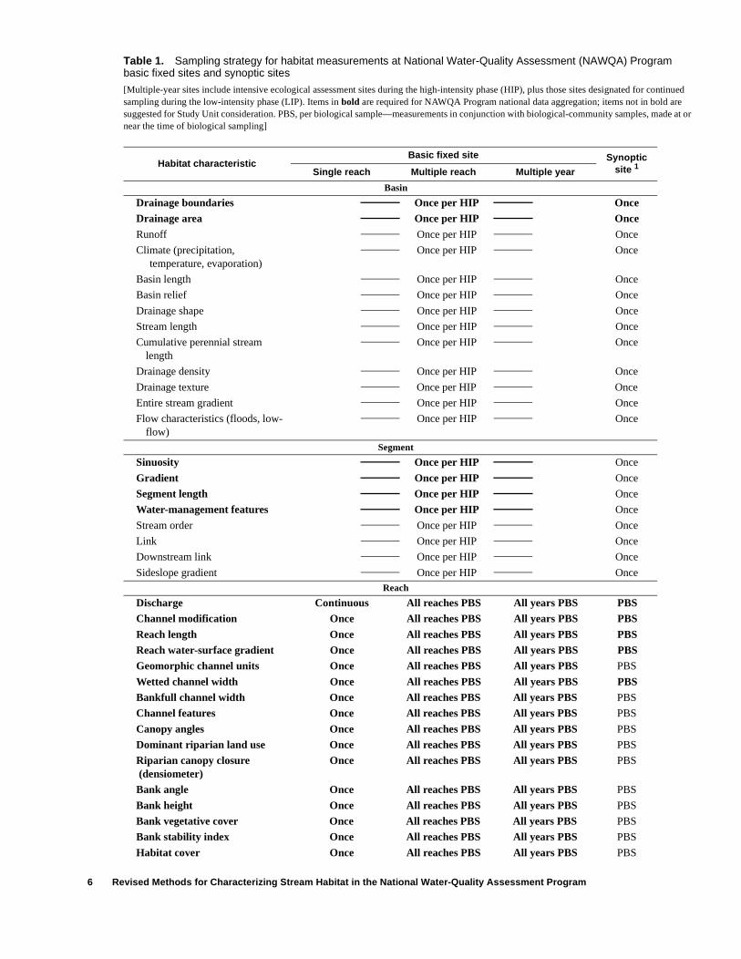
Table 1. Sampling strategy for habitat measurements at National Water-Quality Assessment (NAWQA) Program basic fixed sites and synoptic sites
[Multiple-year sites include intensive ecological assessment sites during the high-intensity phase (HIP), plus those sites designated for continued sampling during the low-intensity phase (LIP). Items in bold are required for NAWQA Program national data aggregation; items not in bold are suggested for Study Unit consideration. PBS, per biological sample—measurements in conjunction with biological-community samples, made at or near the time of biological sampling]
Habitat characteristicBasic fixed site Synoptic
site 1Single reach Multiple reach Multiple year
Basin
Drainage boundaries Once per HIP Once Drainage area Once per HIP Once
Runoff Once per HIP Once
Climate (precipitation,temperature, evaporation)
Once per HIP Once
Basin length Once per HIP Once
Basin relief Once per HIP Once
Drainage shape Once per HIP Once
Stream length Once per HIP Once
Cumulative perennial stream length
Once per HIP Once
Drainage density Once per HIP Once
Drainage texture Once per HIP Once
Entire stream gradient Once per HIP Once
Flow characteristics (floods, low-flow)
Once per HIP Once
Segment
Sinuosity Once per HIP Once
Gradient Once per HIP Once
Segment length Once per HIP Once
Water-management features Once per HIP Once
Stream order Once per HIP Once
Link Once per HIP Once
Downstream link Once per HIP Once
Sideslope gradient Once per HIP OnceReach
Discharge Continuous All reaches PBS All years PBS PBS Channel modification Once All reaches PBS All years PBS PBS
Reach length Once All reaches PBS All years PBS PBS Reach water-surface gradient Once All reaches PBS All years PBS PBS Geomorphic channel units Once All reaches PBS All years PBS PBS
Wetted channel width Once All reaches PBS All years PBS PBS Bankfull channel width Once All reaches PBS All years PBS PBS
Channel features Once All reaches PBS All years PBS PBS
Canopy angles Once All reaches PBS All years PBS PBS
Dominant riparian land use Once All reaches PBS All years PBS PBS
Riparian canopy closure (densiometer)
Once All reaches PBS All years PBS PBS
Bank angle Once All reaches PBS All years PBS PBS
Bank height Once All reaches PBS All years PBS PBS
Bank vegetative cover Once All reaches PBS All years PBS PBS
Bank stability index Once All reaches PBS All years PBS PBS
Habitat cover Once All reaches PBS All years PBS PBS
6 Revised Methods for Characterizing Stream Habitat in the National Water-Quality Assessment Program

Depth Once All reaches PBS All years PBS PBS Velocity Once All reaches PBS All years PBS PBS
Dominant bed substrate Once All reaches PBS All years PBS PBS Embeddedness Once All reaches PBS All years PBS PBS
Bank erosion Once All reaches PBS All years PBS PBS
Siltation Once All reaches PBS All years PBS PBS
Channel cross sections Once Primary reach Once2 PBS
Pebble counts Once All reaches PBS All years PBS PBS
Sediment laboratory analyses Once All reaches PBS All years PBS PBS
Point-quarter vegetation Once Primary reach Once PBS
Vegetation plots Once Primary reach Once PBS1Additional elements may be considered at synoptic sites in conjunction with biological-community sampling, depending on
specific Study Unit objectives.2Once per NAWQA cycle (HIP + LIP), preferably early during the HIP; measurements may be repeated following extremely high-
flow conditions thought to have caused major geomorphic changes.
Table 1. Sampling strategy for habitat measurements at National Water-Quality Assessment (NAWQA) Program basic fixed sites and synoptic sites—Continued
[Multiple-year sites include intensive ecological assessment sites during the high-intensity phase (HIP), plus those sites designated for continued sampling during the low-intensity phase (LIP). Items in bold are required for NAWQA Program national data aggregation; items not in bold are suggested for Study Unit consideration. PBS, per biological sample—measurements in conjunction with biological-community samples, made at or near the time of biological sampling]
Habitat characteristicBasic fixed site Synoptic
site 1Single reach Multiple reach Multiple year
measurements of length and elevation gathered from important basis from which to understand the
USGS 7.5-minute topographic maps, data may need to be collected in inch-pound units because of equipment limitations; however, inch-pound units should be converted into metric units when the data are entered into the computer data base.BASIN CHARACTERIZATION
The characteristics of a stream are dependent in large part upon the downstream transfer of water, sediment, nutrients, and organic material. In order to characterize a stream, it is important to know the geologic, climatic, hydrologic, morphologic, and vegetational setting of a stream within its basin (Schumm and Lichty, 1965; Frissell and others, 1986; Klingeman and MacArthur, 1990). Geology influences the shapes of drainage patterns, channel bed materials, and water chemistry. Soils influence infiltration rates, erosion potential, and vegetation types. Climate affects hydrologic, morphologic, and vegetational characteristics. Vegetation affects a number of factors, including water loss through evapotranspiration, runoff, and channel bank stability. Thus, the basin serves as a fundamental ecosystem unit and an
characteristics of streams (Leopold and others, 1964; Schumm and Lichty, 1965; Frissell and others, 1986; Gordon and others, 1992). Evaluation of basin characteristics also enhances an understanding of the comparative biogeographic patterns in biological communities (Biggs and others, 1990; Quinn and Hickey, 1990).
Background
Basin characterization consists of a combination of (1) geomorphic descriptors using index or ratio data derived from USGS 7.5-minute topographic maps (table 2), (2) climate and potential runoff characteristics, (3) streamflow characteristics for various recurrence intervals, and (4) land-cover data from thematic maps. For NAWQA national data aggregation, the Study Unit is required to delineate and digitize basin boundaries and record methodology. From this information, many of the land-cover data from thematic maps and climate data will be derived by NAWQA national synthesis teams. Although not required for NAWQA national data aggregation, many of the geomorphic descriptors and streamflow
Basin Characterization 7
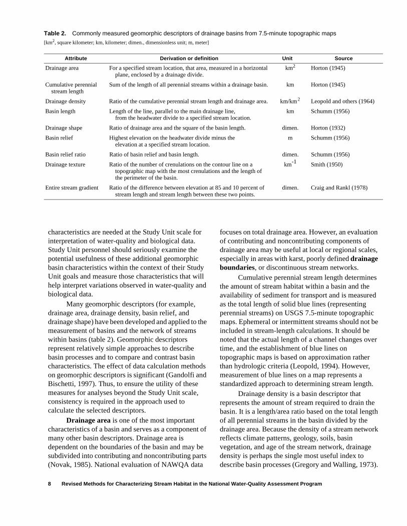
Table 2. Commonly measured geomorphic descriptors of drainage basins from 7.5-minute topographic maps
[km2, square kilometer; km, kilometer; dimen., dimensionless unit; m, meter]
Attribute Derivation or definition Unit Source
Drainage area For a specified stream location, that area, measured in a horizontal plane, enclosed by a drainage divide.
km2 Horton (1945)
Cumulative perennial stream length
Sum of the length of all perennial streams within a drainage basin. km Horton (1945)
Drainage density Ratio of the cumulative perennial stream length and drainage area. km/km2 Leopold and others (1964)
Basin length Length of the line, parallel to the main drainage line, from the headwater divide to a specified stream location.
km Schumm (1956)
Drainage shape Ratio of drainage area and the square of the basin length. dimen. Horton (1932)
Basin relief Highest elevation on the headwater divide minus theelevation at a specified stream location.
m Schumm (1956)
Basin relief ratio Ratio of basin relief and basin length. dimen. Schumm (1956)
Drainage texture Ratio of the number of crenulations on the contour line on a topographic map with the most crenulations and the length of the perimeter of the basin.
km-1 Smith (1950)
Entire stream gradient Ratio of the difference between elevation at 85 and 10 percent of stream length and stream length between these two points.
dimen. Craig and Rankl (1978)
characteristics are needed at the Study Unit scale for interpretation of water-quality and biological data. Study Unit personnel should seriously examine the potential usefulness of these additional geomorphic basin characteristics within the context of their Study Unit goals and measure those characteristics that will help interpret variations observed in water-quality and biological data.
Many geomorphic descriptors (for example, drainage area, drainage density, basin relief, and drainage shape) have been developed and applied to the measurement of basins and the network of streams within basins (table 2). Geomorphic descriptors represent relatively simple approaches to describe basin processes and to compare and contrast basin characteristics. The effect of data calculation methods on geomorphic descriptors is significant (Gandolfi and Bischetti, 1997). Thus, to ensure the utility of these measures for analyses beyond the Study Unit scale, consistency is required in the approach used to calculate the selected descriptors.
Drainage area is one of the most important characteristics of a basin and serves as a component of many other basin descriptors. Drainage area is dependent on the boundaries of the basin and may be subdivided into contributing and noncontributing parts (Novak, 1985). National evaluation of NAWQA data
focuses on total drainage area. However, an evaluation of contributing and noncontributing components of drainage area may be useful at local or regional scales, especially in areas with karst, poorly defined drainage boundaries, or discontinuous stream networks.
Cumulative perennial stream length determines the amount of stream habitat within a basin and the availability of sediment for transport and is measured as the total length of solid blue lines (representing perennial streams) on USGS 7.5-minute topographic maps. Ephemeral or intermittent streams should not be included in stream-length calculations. It should be noted that the actual length of a channel changes over time, and the establishment of blue lines on topographic maps is based on approximation rather than hydrologic criteria (Leopold, 1994). However, measurement of blue lines on a map represents a standardized approach to determining stream length.
Drainage density is a basin descriptor that represents the amount of stream required to drain the basin. It is a length/area ratio based on the total length of all perennial streams in the basin divided by the drainage area. Because the density of a stream network reflects climate patterns, geology, soils, basin vegetation, and age of the stream network, drainage density is perhaps the single most useful index to describe basin processes (Gregory and Walling, 1973).
8 Revised Methods for Characterizing Stream Habitat in the National Water-Quality Assessment Program

High drainage density may indicate high flood peaks, high sediment production, steep hillslopes, general difficulty of access, low suitability for agriculture, and high construction costs. Drainage density ranges from about 1 to 1,000 (Leopold and others, 1964).
There are many methods used to measure basin length (Gardiner, 1975). The definition given by Schumm (1956) is used here, where a line is drawn from the mouth of the basin following the main stream valley to the drainage divide. Basin length is used for calculating drainage shape.
Drainage shape is a ratio designed to convey information about the elongation of a basin. Drainage shape is difficult to express unambiguously and has been measured several different ways (Gordon and others, 1992). The definition for basin shape as originally proposed by Horton (1932) is used here, where drainage shape is a simple dimensionless ratio of drainage area divided by the square of basin length. In general, with increasing drainage area, basins tend to increase in length faster than in width. Given two drainage basins of the same size, an elongated basin will tend to have smaller flood peaks but longer lasting floodflows than a round basin (Gregory and Walling, 1973).
Basin relief can have a significant effect on drainage density and stream gradient. Hadley and Schumm (1961) demonstrated that annual sediment yields increase exponentially with basin relief. The basin relief ratio (basin relief divided by basin length) (Schumm, 1956) is helpful for eliminating the effects of differences in basin size when comparing data from drainage basins of different size.
Drainage texture represents a measure of the proximity of streams in a basin. Although two basins may have the same or similar drainage densities, the basins may differ in texture or the dissection of streams within the basin. For example, the cumulative length of streams may be the same in two basins, but the number of streams may be different. Smith (1950) developed a ratio by dividing the number of crenulations (taken from the contour with the most crenulations in the basin on a USGS 7.5-minute topographic map) by the length of the perimeter of the basin. The crenulations are an indication of channel crossing and, thus, a measure of the closeness of the spacing between streams. It is recognized that the determination of drainage texture from 7.5-minute maps can be difficult for relatively large drainage areas.
A measurement of the entire stream gradient (Craig and Rankl, 1978) is used in estimations of flood characteristics. Along with drainage area, this characteristic is one of the most important characteristics used to estimate the size of floods. It may be quite different from channel gradient, which is measured at the segment scale. To measure entire stream gradient, points at 85 percent and 10 percent of the basin length, as measured from the mouth of the basin, are determined. Elevations at these points are determined and subtracted. The resulting difference is then divided by 75 percent of the basin length.
A computer program called "Basinsoft" has been developed by the USGS to quantify a number of basin characteristics, such as the ones described above, by using GIS information (Eash, 1994; Harvey and Eash, 1996). Basinsoft uses four digital maps (drainage-basin boundary, hydrography extracted from digital line-graph data, hypsography generated from digital elevation-model data, and a lattice elevation model generated from digital elevation-model data) to quantify 27 basin characteristics (table 3). Comparison tests indicate that, for most characteristics, Basinsoft-generated descriptors of basins are not significantly different from those calculated manually from 7.5-minute topographic maps. However, comparison tests indicate that descriptors that rely on measures of slope, such as basin relief, are underestimated by Basinsoft. Additional information regarding the Basinsoft processing steps is provided by Harvey and Eash (1996).
Even though all the geomorphic descriptors except drainage area are optional for NAWQA data aggregation, most descriptors will be important for Study Unit analyses of relations among drainage basin geomorphology, instream channel characteristics, biotic assemblages, and water chemistry. For example, in a study of the relations of geomorphology to trout populations in Rocky Mountain streams, Lanka and others (1987) demonstrated significant correlations among measures of drainage basin geomorphology, instream habitat, and trout abundance. These investigators reported significant univariate correlations among basin relief, drainage density, stream length, and reach-scale habitat characteristics in both high-elevation forest and low-elevation rangeland streams (Lanka and others, 1987). They also found that multiple-regression equations predicting fish abundance were often dominated by basin geomorphic descriptors, with some descriptors predicting fish
Basin Characterization 9
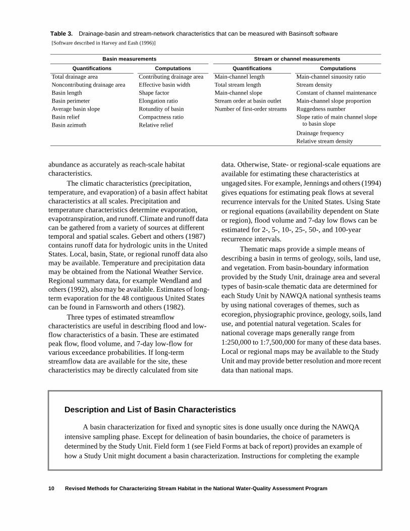
Table 3. Drainage-basin and stream-network characteristics that can be measured with Basinsoft software
[Software described in Harvey and Eash (1996)]
Basin measurements Stream or channel measurements
Quantifications Computations Quantifications Computations
Total drainage area Contributing drainage area Main-channel length Main-channel sinuosity ratioNoncontributing drainage area Effective basin width Total stream length Stream densityBasin length Shape factor Main-channel slope Constant of channel maintenanceBasin perimeter Elongation ratio Stream order at basin outlet Main-channel slope proportionAverage basin slope Rotundity of basin Number of first-order streams Ruggedness numberBasin relief Compactness ratio Slope ratio of main channel slope
to basin slopeBasin azimuth Relative reliefDrainage frequencyRelative stream density
abundance as accurately as reach-scale habitat characteristics.
The climatic characteristics (precipitation, temperature, and evaporation) of a basin affect habitat characteristics at all scales. Precipitation and temperature characteristics determine evaporation, evapotranspiration, and runoff. Climate and runoff data can be gathered from a variety of sources at different temporal and spatial scales. Gebert and others (1987) contains runoff data for hydrologic units in the United States. Local, basin, State, or regional runoff data also may be available. Temperature and precipitation data may be obtained from the National Weather Service. Regional summary data, for example Wendland and others (1992), also may be available. Estimates of long-term evaporation for the 48 contiguous United States can be found in Farnsworth and others (1982).
Three types of estimated streamflow characteristics are useful in describing flood and low-flow characteristics of a basin. These are estimated peak flow, flood volume, and 7-day low-flow for various exceedance probabilities. If long-term streamflow data are available for the site, these characteristics may be directly calculated from site
data. Otherwise, State- or regional-scale equations are available for estimating these characteristics at ungaged sites. For example, Jennings and others (1994) gives equations for estimating peak flows at several recurrence intervals for the United States. Using State or regional equations (availability dependent on State or region), flood volume and 7-day low flows can be estimated for 2-, 5-, 10-, 25-, 50-, and 100-year recurrence intervals.
Thematic maps provide a simple means of describing a basin in terms of geology, soils, land use, and vegetation. From basin-boundary information provided by the Study Unit, drainage area and several types of basin-scale thematic data are determined for each Study Unit by NAWQA national synthesis teams by using national coverages of themes, such as ecoregion, physiographic province, geology, soils, land use, and potential natural vegetation. Scales for national coverage maps generally range from 1:250,000 to 1:7,500,000 for many of these data bases. Local or regional maps may be available to the Study Unit and may provide better resolution and more recent data than national maps.
10
Description and List of Basin Characteristics
A basin characterization for fixed and synoptic sites is done usually once during the NAWQA intensive sampling phase. Except for delineation of basin boundaries, the choice of parameters is determined by the Study Unit. Field form 1 (see Field Forms at back of report) provides an example of how a Study Unit might document a basin characterization. Instructions for completing the example
Revised Methods for Characterizing Stream Habitat in the National Water-Quality Assessment Program
d for
ive
r
aber king
s a
inutes, a s often .
each
r each ndix
bases.
.
r the
re basin
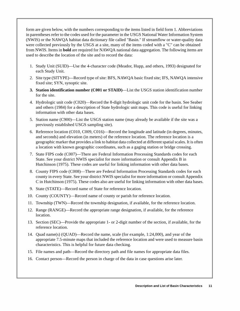
form are given below, with the numbers corresponding to the items listed in field form 1. Abbreviations in parentheses refer to the codes used for the parameter in the USGS National Water Information System (NWIS) or the NAWQA habitat data dictionary file called "Basin." If streamflow or water-quality data were collected previously by the USGS at a site, many of the items coded with a "C" can be obtained from NWIS. Items in bold are required for NAWQA national data aggregation. The following items are used to describe the location of the site and to record the data:
1. Study Unit (SUID)—Use the 4-character code (Meador, Hupp, and others, 1993) designateeach Study Unit.
2. Site type (SITYPE)—Record type of site: BFS, NAWQA basic fixed site; IFS, NAWQA intensfixed site; SYN, synoptic site.
3. Station identification number (C001 or STAID)—List the USGS station identification numbefor the site.
4. Hydrologic unit code (C020)—Record the 8-digit hydrologic unit code for the basin. See Seand others (1984) for a description of State hydrologic unit maps. This code is useful for lininformation with other data bases.
5. Station name (C900)—List the USGS station name (may already be available if the site wapreviously established USGS sampling site).
6. Reference location (C010, C009, C016)—Record the longitude and latitude (in degrees, mand seconds) and elevation (in meters) of the reference location. The reference location isgeographic marker that provides a link to habitat data collected at different spatial scales. It ia location with known geographic coordinates, such as a gaging station or bridge crossing
7. State FIPS code (C007)—There are Federal Information Processing Standards codes for State. See your district NWIS specialist for more information or consult Appendix B in Hutchinson (1975). These codes are useful for linking information with other data bases.
8. County FIPS code (C008)—There are Federal Information Processing Standards codes focounty in every State. See your district NWIS specialist for more information or consult AppeC in Hutchinson (1975). These codes also are useful for linking information with other data
9. State (STATE)—Record name of State for reference location.
10. County (COUNTY)—Record name of county or parish for reference location.
11. Township (TWN)—Record the township designation, if available, for the reference location
12. Range (RANGE)—Record the appropriate range designation, if available, for the referencelocation.
13. Section (SEC)—Provide the appropriate 1- or 2-digit number of the section, if available, foreference location.
14. Quad name(s) (QUAD)—Record the name, scale (for example, 1:24,000), and year of theappropriate 7.5-minute maps that included the reference location and were used to measucharacteristics. This is helpful for future data checking.
15. File names and path—Record the directory path and file names for appropriate data files.
16. Contact person—Record the person in charge of the data in case questions arise later.
Description and List of Basin Characteristics 11

12
a in ds are
ge nt.
urces duced imated rs) and
m USGS l data
GE, HER.
cord verage
elsius) States.
hers, given ral
es vered
s ted
n;
The following basin characteristics can be computed by using GIS, Basinsoft, or manual methods, and most are stored in the data dictionary file called "Basin":17. Total drainage area (C808)—Delineate basin boundaries and calculate the total drainage are
square kilometers (> 0.0) of the basin upstream from the site. Both manual and GIS methopossible, using various map scales. It is worthwhile to record contributing (C809) area, if applicable.
18. Drainage area method (DRAREAMD)—This pertains to the method used to determine drainaarea. Record the map year, computation method, source map scale used for the assessme
19. Average annual runoff (RUNOFF)—Runoff information can be gathered from a variety of soat different scales. Maps of runoff for the hydrologic units in the United States have been proby Gebert and others (1987). Average annual runoff (reported in centimeters) usually is estby dividing average streamflow (cubic meters per second) by the drainage area (square metemultiplying by the number of seconds in a year (60 x 60 x 24 x 365) and the conversion frocentimeters to meters (100 cm/m). Numerous publications also have been published by thefor major river basins (one example for Wisconsin is Skinner and Borman, 1973). More locamay also be available.
20. Average annual runoff method (RUNOFFMD)—Record the method used. Methods includeGAGE, calculations from long-term streamflow record (gaging station) at the station; WTGAarea weighting multiple gaging stations; REFERENCE, value from published source; or OT
21. Beginning and ending years of record for runoff data (BYRUNOFF and EYRUNOFF)—Rethe beginning and ending years for runoff calculations. Because these data are based on aannual streamflow, it is important to know the length of record used for the calculations.
22. Average annual air temperature (TEMP)—Data for average annual temperature (degrees Ccan be gathered from some National Weather Service precipitation gages across the UnitedConsult your State climatologist or the nearest National Weather Service office for more information. Regional summary data also may be available (for example, Wendland and ot1992). At the highest scale of detail, data from several weather stations are averaged for adrainage basin. Collect data from stations within and surrounding the drainage basin. Sevemethods can be used:
a. Construct Thiessen polygons by connecting nearest-neighbor stations and drawing linperpendicular to them, and weight temperature at a station by the proportion of area coin the drainage basin;
b. Calculate grid-weighted average created from nearest-neighbor computation;
c. Draw contour lines of equal temperature (isohyets);
d. Obtain value from published sources;
e. Calculate the arithmetic mean temperature for all the weather stations in the basin;
f. Calculate a grid-weighted average created from kriging computation; and
g. Other.
See Dunne and Leopold (1978, p. 37–42) for more detailed instructions.
23. Average annual air temperature method (TEMPMD)—The domain for this variable includeTHIESSEN, area-weighted average from irregularly spaced points; NEIGHBOR, grid-weighaverage created from nearest-neighbor computation; ISOHYET, value from contour lines; REFERENCE, value from published source; AVG, arithmetic mean from all stations in basi
Revised Methods for Characterizing Stream Habitat in the National Water-Quality Assessment Program

s is used.
d from m ove on ong
mine , area-ted lue hted es
This riod
Unit. 48
sed to
hted
in; s not
line rdiner
ngth.
ove 0).
le used
KRIG, grid-weighted average created from kriging computation; OTHER, method used was not one of the choices listed.
24. Beginning and ending years of record for temperature data (BYTEMP and EYTEMP)—Thivery important information to record because results will vary depending on the time period
25. Average annual precipitation (PRECIP)—An area-weighted average in centimeters obtainemost recent (or most accurate) reports or studies describing the basin or data gathered froNational Weather Service precipitation stations. For calculating averages, see discussion abaverage annual air temperature. The sources, scale, and quality of these data will vary amStudy Units and basins.
26. Average annual precipitation method (PRECIPMD)—Pertains to the method used to deteraverage annual precipitation in the basin. The domain for this variable includes THIESSENweighted average from irregularly spaced points; NEIGHBOR, grid-weighted average creafrom nearest-neighbor computation; ISOHYET, value from contour lines; REFERENCE, vafrom published source; AVG, arithmetic mean from all stations in the basin; KRIG, grid-weigaverage created from kriging computation; OTHER, method used was not one of the choiclisted.
27. Beginning and ending years of record for precipitation data (BYPRECIP and EYPRECIP)—is very important information to record, because results will vary depending on the time peused.
28. Average annual Class A pan evaporation (EVAPAN)—This value is often an area-weightedaverage, in centimeters. Available data will vary in source, scale, and quality for each StudyEstimates of long-term evaporation and free-water surface evaporation for the contiguous United States are found in Farnsworth and others (1982).
29. Average annual Class A pan evaporation method (EVAPANMD)—Pertains to the method udetermine average annual evaporation in the basin. The domain for this variable includes THIESSEN, area-weighted average from irregularly spaced points; NEIGHBOR, grid-weigaverage created from nearest-neighbor computation; ISOHYET, value from contour lines; REFERENCE, value from published source; AVG, arithmetic mean from all stations in basKRIG, grid-weighted average created from kriging computation; OTHER, method used waone of the choices listed.
30. Beginning and ending years of record for evaporation data (BYEVAPAN and EYEVAPAN)—Record beginning and ending dates of data sets, because results will vary depending on the time period used.
31. Basin length (BLENG)—Measure the length of the basin in kilometers (> 0.0) by drawing afrom the mouth of the basin following the main stream valley to the drainage divide. See Ga(1975) for examples of how to calculate basin length.
32. Basin length method (BLENGMD)—This pertains to the method used to determine basin leRecord the map year, computation method, source map scale used for the assessment.
33. Minimum elevation in the basin (MNELEV)—Determine the minimum elevation in meters abthe 1929 National Geodetic Vertical Datum (NGVD) (above datum > 0.0; below datum < 0.
34. Minimum elevation method (MNELEVMD)—This pertains to the method used to determineminimum elevation in the basin. Record the map year, computation method, source map scafor the assessment.
Description and List of Basin Characteristics 13

14
ove
e le used
.
. Units
ent.
ers
sed to source
Units
noted e the eter.
ercent e two
s are flow,
ristics w e btain s can QP10, ar ated 00). sed
flow
35. Maximum elevation in the basin (MXELEV)—Determine the maximum elevation in meters abNGVD (above datum > 0.0; below datum < 0.0).
36. Maximum elevation method (MXELEVMD)—This pertains to the method used to determinmaximum elevation in the basin. Record the map year, computation method, source map scafor the assessment.
37. Basin relief ratio (RELRAT)—Determine the difference between the MXELEV and MNELEVDivide the difference by BLENG.
38. Drainage shape (DRNSHAPE)—Divide the drainage area by the square of the basin lengthare dimensionless.
39. Stream length (SLENG)—Measure the longest stream length in kilometers (> 0.0) from theheadwaters to the site.
40. Stream length method (SLENGMD)—This pertains to the method used to determine streamlength. Record the map year, computation method, source map scale used for the assessm
41. Cumulative perennial stream length (PSLENG)—Measure the cumulative length in kilomet(> 0.0) of all perennial streams and canals in the basin.
42. Cumulative perennial stream length method (PSLENGMD)—This pertains to the method udetermine cumulative perennial stream length. Record the map year, computation method,map scale used for the assessment.
43. Drainage density (DRNDENS)—Divide the cumulative stream length by the drainage area.are kilometer-1.
44. Drainage texture (DRNTEX)—Determine the basin contour with the most crenulations, as by inspection of a 7.5-minute map. Count the number of crenulations on that contour. Dividnumber of crenulations by the length of the perimeter of the basin. Units are contours/kilom
45. Entire stream gradient (SLOPE)—A ratio of the difference between elevation at 85 and 10 pof stream length as measured from the reference location and stream length between thespoints (Craig and Rankl, 1978). Units are recorded in meters per kilometer.
46. Estimated flow characteristics—At least three types of estimated streamflow characteristicuseful for describing flood and low-flow characteristics of a basin. They are estimated peakflood volume, and 7-day low-flow for given recurrence intervals. If the site has long-term streamflow data (5–15 years of data, depending on the recurrence interval), these charactecan be directly calculated. USGS District offices also can provide statistical analyses for flocharacterization at USGS gaging stations. Otherwise, State- or regional-scale equations aravailable for estimating these characteristics (for example, Jennings and others (1994) to oequations for estimating peak flows for specific hydrologic regions within a State). Peak flowbe estimated for 1-, 2-, 5-, 10-, 25-, 50-, and 100-year recurrence intervals (QP1, QP2, QP5,QP25, QP50, QP100). Flood volume can be estimated for 2-, 5-, 10-, 25-, 50-, and 100-yeintervals (QV2, QV5, QV10, QV25, QV50, QV100). In addition, 7-day low flows can be estimfor 2-, 5-, 10-, 25-, 50-, and 100-year intervals (Q7L2, Q7L5, Q7L10, Q7L25, Q7L50, Q7L1Be sure to record beginning (QBDATE) and ending (QEDATE) dates of streamflow record uto estimate these characteristics, if applicable.
47. Method used to estimate flow characteristics (FLOWMD)—Record method used to estimate
Revised Methods for Characterizing Stream Habitat in the National Water-Quality Assessment Program

he
ent
nd
,
ed o are
ly d
be r in
,
try
characteristics, such as streamflow data from a gaging station or reference source for equations.
Many types of ancillary basin data in a GIS may be associated with water quality. A short description and some sources for GIS data that can be collected but are not included on the basin form are listed below. Two useful measurements are percentage of basin covered and absolute area (such as square kilometers). Even though these data may be in a computerized format from the start, it is very important to record data sources, scale, category definitions, date, and spatial extent. These data are stored in the habitat dictionary files called "Giscat" and "Cover." Data for several of the thematic maps listed below may be provided to the Study Unit by a NAWQA national synthesis team.
Land use/land cover—Land-use/land-cover information for the Nation is available from USGS high-altitude color-infrared aerial photography generally taken in the 1970’s at a scale of 1:250,000. The land-use/land-cover classification scheme used is based on Anderson and others (1976). Additional land-use/land-cover GIS maps from other sources are available at a higher resolution for some areas.
Soils—The State soil geographic data base (STATGO) is available for the United States and contains general information on soil texture, permeability, and erodibility at a scale of 1:250,000. See U.S. Department of Agriculture (1991) for more details.
Geology—GIS coverages are available for bedrock and surficial geology but will differ in spatial extent and scale for each Study Unit. A national map of bedrock geology (King and Beikman, 1974) at a scale of 1:2,500,000 is available from GIS data bases. Consult applicable State geological surveys for more information.
Physiography—A national GIS coverage of physiography for the United States is available at a scale of 1:7,000,000. Provinces and sections are based on common topography, bedrock type and structure, and geologic and geomorphic history (Fenneman, 1946).
Ecoregions—A national GIS coverage of ecoregions in the United States is available at a scale of 1:7,500,000, based on overlays of land use, major land-resource areas, and natural vegetation types. See Omernik (1987) and Hughes and Larsen (1988) for more information. Revised and regional
maps also may be available. Be sure to record tdate of the map.
Potential natural vegetation—A national GIS coverage of vegetation before European settlem(Küchler, 1970) for the United States is availableat a scale of 1:7,500,000.
Land-resource areas—A national GIS coverage of land-resource areas for the United States is available at a scale of 1:7,500,000. The land-resource areas are based on the interrelation of lause, climate, water resources, and soils (U.S. Department of Agriculture, 1972).
Wetlands—The U.S. Fish and Wildlife Service’s National Wetlands Inventory is designed to determine the status of and trends in wetlands throughout the United States (Frayer and others1983; Dahl and Johnson, 1991). Wetlands are defined on the basis of plant types, soils, and frequency of flooding. Approximately 80 percentof wetlands in the United States have been mappat 1:24,000-scale resolution. Approximately 20 t30 percent of the maps have been digitized and available in the Map Overlay Statistical System (MOSS) format.
SEGMENT CHARACTERIZATION
A segment is a length of stream that is relativehomogeneous with respect to physical, chemical, anbiological properties. Boundaries of a segment may tributary junctions that contain different streamflow owater-quality characteristics or substantial changes basin characteristics (fig. 1) or major hydrologic discontinuities, such as waterfalls, landform featuressignificant changes in gradient, or point-source discharges (Frissell and others, 1986). Water-chemispatterns (Teti, 1984) and benthic-invertebrate communities (Burns and others, 1984) have been shown to vary where tributaries converge.
Background
Gradient, sinuosity, and water-management features are required elements for NAWQA national data aggregation. Additional information, including Strahler stream order, link (Shreve stream order), downstream link, sideslope gradient, and riparian
Segment Characterization 15

vegetation, may be important for Study Unit analyses of biological and water-quality conditions.
Gradient is the ratio of channel-elevation drop divided by the curvilinear channel length. It is an indication of the amount of energy available for movement of water and sediment through the reach; thus, it has a direct influence on streamflow and channel substrate characteristics and on the type of aquatic habitat present. Gradient can be an important determinant in the distribution of fish (Maret and others, 1997) and invertebrates (Tate and Heiny, 1995).
Sinuosity describes the channel pattern. It is the ratio of curvilinear channel length to the valley centerline length (Schumm, 1963; Platts and others, 1983) (fig. 2). For sinuous channels tightly confined in V-shaped valleys, straight-line segments that follow the broad-scale changes in channel direction can be substituted for the valley centerline length (Gordon and others, 1992). It is important to note that sinuosity is dependent on the length of stream measured. For most situations, the segment length should be used. If the segment is very short, a curvilinear channel length of at least 20 times the bankfull width of the stream should be measured (Gordon and others, 1992). In meandering streams, 20 times the bankfull width incorporates at least 1 meander wavelength (Leopold and others, 1964). Straight streams will have a sinuosity of 1,
whereas meandering streams generally have a sinuosity of 1.5 or more (Leopold and others, 1964). Sinuosity is helpful in describing energy conditions and is related to gradient and the diversity of habitat. In general, low sinuosity indicates a steep channel gradient, uniform cross sections, and few pools. High sinuosity is associated with flat gradients, asymmetrical cross sections, overhanging banks, and pools on the outside bend of meanders.
Water-management features are local hydrologic features that may cause temporal or spatial variability of habitat and water-quality characteristics in the segment. They include bridges, channelization, diversions, point sources, tile drains, bank stabilization, lakes, dams, and any other features that may be important. These features may form the boundaries of the segment. In addition, features outside of the segment boundaries should be noted if they might be affecting habitat or water quality within the segment.
Stream order, or classification of streams based on the number and type of tributary junctions, has proven to be a useful indicator of stream size, discharge, and drainage area (Strahler, 1957). There are several methods for determining stream order. Two commonly used methods are the Strahler method (Strahler, 1957) and the link, or Shreve method
16 Revised Methods for Characterizing Stream Habitat in the National Water-Quality Assessment Program
valley wall
meandering channel
valley centerline
length of channel
length of valley centerlineSinuosity =
valley wall
meander length
(wave length)
Figure 2. Example of how to measure sinuosity.
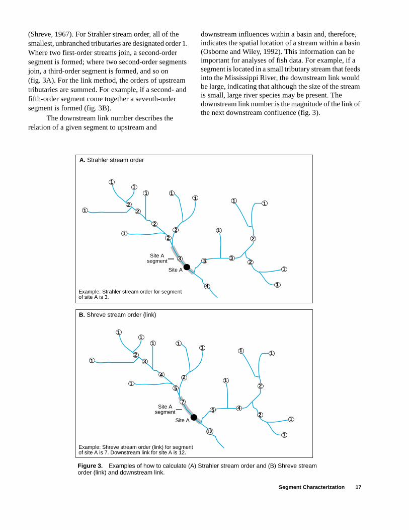
(Shreve, 1967). For Strahler stream order, all of the smallest, unbranched tributaries are designated order 1. Where two first-order streams join, a second-order segment is formed; where two second-order segments join, a third-order segment is formed, and so on (fig. 3A). For the link method, the orders of upstream tributaries are summed. For example, if a second- and fifth-order segment come together a seventh-order segment is formed (fig. 3B).
The downstream link number describes the relation of a given segment to upstream and
downstream influences within a basin and, therefore, indicates the spatial location of a stream within a basin (Osborne and Wiley, 1992). This information can be important for analyses of fish data. For example, if a segment is located in a small tributary stream that feeds into the Mississippi River, the downstream link would be large, indicating that although the size of the stream is small, large river species may be present. The downstream link number is the magnitude of the link of the next downstream confluence (fig. 3).
Segment Characterization 17
Figure 3. Examples of how to calculate (A) Strahler stream order and (B) Shreve stream order (link) and downstream link.
Site A
1
1
1
11 1
1
1 1
1
1 122
22
3
2
233
4
Site A
Site Asegment
2
Site Asegment
Example: Strahler stream order for segmentof site A is 3.
Example: Shreve stream order (link) for segmentof site A is 7. Downstream link for site A is 12.
B. Shreve stream order (link)
A. Strahler stream order
1
1
1
11 1
1
1 1
1
1 1
2
23
4
5
7
2
245
12
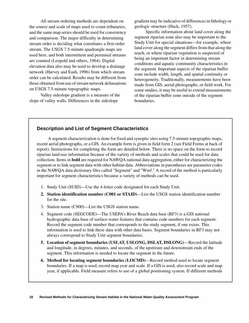
All stream ordering methods are dependent on the source and scale of maps used to count tributaries, and the same map series should be used for consistency and comparison. The major difficulty in determining stream order is deciding what constitutes a first-order stream. The USGS 7.5-minute quadrangle maps are used here, and both intermittent and perennial streams are counted (Leopold and others, 1964). Digital elevation data also may be used to develop a drainage network (Harvey and Eash, 1996) from which stream order can be calculated. Results may be different from those obtained from use of stream network delineations on USGS 7.5-minute topographic maps.
Valley sideslope gradient is a measure of the
gradient may be indicative of differences in lithology or geologic structure (Hack, 1957).
Specific information about land cover along the segment riparian zone also may be important to the Study Unit for special situations—for example, where land cover along the segment differs from that along the reach, or where riparian vegetation is suspected of being an important factor in determining stream conditions and aquatic community characteristics in the segment. Important aspects of the riparian buffer zone include width, length, and spatial continuity or heterogeneity. Traditionally, measurements have been made from GIS, aerial photographs, or field work. For some studies, it may be useful to extend measurements of the riparian buffer zone outside of the segment
18
slope of valley walls. Differences in the sideslope boundaries.
Description and List of Segment Characteristics
A segment characterization is done for fixed and synoptic sites using 7.5-minute topographic maps, recent aerial photographs, or a GIS. An example form is given in field form 2 (see Field Forms at back of report). Instructions for completing the form are detailed below. There is no space on the form to record riparian land-use information because of the variety of methods and scales that could be used for data collection. Items in bold are required for NAWQA national data aggregation, either for characterizing the segment or to link segment data with other habitat data. Abbreviations in parentheses are parameter codes in the NAWQA data dictionary files called "Segment" and "Wmf." A record of the method is particularly important for segment characteristics because a variety of methods can be used.
1. Study Unit (SUID)—Use the 4-letter code designated for each Study Unit.
2. Station identification number (C001 or STAID)—List the USGS station identification number for the site.
3. Station name (C900)—List the USGS station name.
4. Segment code (SEGCODE)—The USEPA’s River Reach data base (RF3) is a GIS national hydrographic data base of surface-water features that contains code numbers for each segment. Record the segment code number that corresponds to the study segment, if one exists. This information is used to link these data with other data bases. Segment boundaries in RF3 may not always correspond to Study Unit segment boundaries.
5. Location of segment boundaries (USLAT, USLONG, DSLAT, DSLONG)—Record the latitude and longitude, in degrees, minutes, and seconds, of the upstream and downstream ends of the segment. This information is needed to locate the segment in the future.
6. Method for locating segment boundaries (LOCMD)—Record method used to locate segment boundaries. If a map is used, record map year and scale. If a GIS is used, also record scale and map year, if applicable. Field measure refers to use of a global positioning system. If different methods
Revised Methods for Characterizing Stream Habitat in the National Water-Quality Assessment Program

th he s that length
ale and
int of to the ference cation,
ed, also ystem.
m
scale. If global
y e
ll width ill have
old and
t
ce tes, if nce
ent d if they s for
were used to measure longitude and latitude, record differences at the end of the field form in item no. 26. “Comments about segment data.”
7. Segment (valley) length (SEGLENG)—Using a map wheel (or GIS), record the straight-line lengof the segment, in kilometers, by following a relatively straight line through the centerline of tvalley (fig. 2). For sinuous channels tightly confined in V-shaped valleys, straight-line segmentfollow the broad-scale changes in channel direction can be substituted for the valley centerline(Gordon and others, 1992).
8. Method used to measure segment length (SEGLENMD)—Record method used to measure segment length. If a map is used, record map year and scale. If a GIS is used, also record scmap year, if applicable. Field measure refers to use of a global positioning system.
9. Curvilinear channel length and distance to reference location (SEGCUR, USDIST, DSDIST)—Using a map wheel (or GIS), record the approximate length, in kilometers, of the channel in the segment by following a line through the thalweg of the main channel (or midpochannel if thalweg is not known). Record the curvilinear distance from the reference location upstream and downstream boundaries of the segment. If the boundary is upstream from the relocation, record it as a negative number. If the boundary is downstream from the reference lorecord it as a positive number.
10. Method used to measure curvilinear channel length (SEGCURMD)—Record method used to measure curvilinear channel length. If a map is used, record map year and scale. If a GIS is usrecord scale and map year, if applicable. Field measure refers to use of a global positioning s
11. Upstream and downstream elevation (USELEV, DSELEV)—Record elevation, in meters, of a segment at upstream and downstream boundaries using the National Geodetic Vertical Datu(NGVD).
12. Method used to measure upstream and downstream elevation (SELEVMD)—Record method used to measure upstream and downstream elevation. If a map is used, record map year anda GIS is used, also record scale and map year, if applicable. Field measure refers to use of apositioning system.
13. Sinuosity (SINUOS)—To calculate sinuosity, divide the curvilinear channel length by the vallelength (fig. 2). If the segment is very short, a curvilinear channel length of at least 20 times thbankfull width of the stream should be measured. In meandering streams, 20 times the bankfuincorporates at least one meander wavelength (Leopold and others, 1964). Straight streams wa sinuosity of 1, whereas meandering streams generally have a sinuosity of 1.5 of more (Leopothers, 1964).
14. Segment gradient (GRADIENT)—Determine the gradient of the segment by subtracting the downstream elevation from the upstream elevation and dividing the difference by the segmenchannel length.
15. Water management feature (WMFID, WMFTYPE, WMFDES, WMFBDATE, WMFEDATE, WMFDIST)—Record the type(s) of water management feature(s) that is(are) likely to influenhabitat conditions in the segment. Include a short description and give starting and ending daappropriate. Record distance from the reference location; distances upstream from the referelocation are negative, and those downstream are positive. Include as many water-managemfeatures as appropriate. Features upstream or downstream from the segment should be notemight be affecting habitat or water quality within the segment. Use the following 12-letter codeWMFTYPE:
Description and List of Segment Characteristics 19
20
nated ent is (fig.
eam
ent , the d may r order
a
ent f the m the
flows the ls and
Data
al ontal e
data;
mes for
.
ts or
Bridge Natural Lake Gw InflowDiversion Bank Stabiliz HydropowerReturn Flow Tile Drain IndustrialStp > 5 None MiningIps > 5 Channelized Storm SewerImpoundment Feedlot ThermalLow-head Dam Sewage Treat Other
16. Strahler stream order (ORDER)—On a USGS 7.5-minute topographic map showing all intermittent and perennial streams in a basin, the smallest unbranched tributaries are desigorder 1 (Leopold and others, 1964). Where two first-order streams join, a second-order segmformed; where two second-order segments join, a third-order segment is formed, and so on3). For irrigation canals and other "artificial" systems, "-1" is recorded for stream order.
17. Strahler stream-order method (ORDERMD)—Record method used to measure Strahler strorder. Data sources include maps or GIS; record year and scale for either type.
18. Link (Shreve stream order) (LINK)—Calculating the link, or Shreve stream order, for a segmis done by summing the orders of upstream tributaries (Shreve, 1967) (fig. 3). For examplejoining of a second-order and third-order stream produces a fifth-order stream. This methobe a better indicator of the approximate size of a drainage basin than the Strahler method,especially if a drainage basin has a large number of minor tributaries that intersect a highestream. For irrigation canals and other manmade systems, "-1" is recorded for link.
19. Link (Shreve stream order) method (LINKMD)—Record method used to measure link. Datsources include maps or GIS. Record year and scale for either type.
20. Downstream link (DSTRLINK)—Calculate the link of the stream downstream from the segmand below the next tributary junction. Downstream link number is the magnitude of the link onext downstream confluence (fig. 3). For example, the segment immediately downstream froconfluence of two headwater tributaries has a downstream link of 2. If a headwater tributaryinto a stream with a downstream link of 2, then the segment immediately downstream fromconfluence of these two streams has a downstream link of 3, and so on. For irrigation canaother manmade systems, "-1" is recorded for downstream link.
21. Downstream link method (DSLINKMD)—Record method used to measure downstream link.sources include maps or GIS; record year and scale for either type.
22. Valley sideslope gradient (SIDEGRAD)—Sideslope gradient is based on the cross-sectionprofile of the segment valley. Make three gradient measurements within 300 m of the horizdistance of the channel at positions representative of the valley sideslope gradient along thsegment. These measurements and their mean are recorded.
23. Method used to measure valley sideslope gradient (SIDEGRMD)—Record method used tomeasure sideslope gradient. Possible methods include map-derived data, field data, or GISrecord map year and scale, if applicable.
24. File names and path name where data can be found—Record the directory path and file naappropriate data files.
25. Contact person for segment data—Record the name of the person responsible for the data
26. Comments about segment data (SEGCOM)—Note special circumstances for measuremendata limitations.
Revised Methods for Characterizing Stream Habitat in the National Water-Quality Assessment Program

ch. l itat tal fic ss
o ree
nd), r r
,
s,
y
es
r
e
w
es m
REACH CHARACTERIZATION
A reach (fig. 1) is the least clearly defined unit in the spatial hierarchy; however, it is the most useful scale for describing long-term effects of human activities and determining population and distribution of aquatic communities (Frissell and others, 1986). Although a segment is a discrete unit that should represent a uniform set of physical, chemical, and biological conditions within a stream, its length (often more than several kilometers) prohibits effective collection of field data. The reach is the principal sampling unit for collecting physical, chemical, and biological data that represent conditions within the segment.
Selection of a Reach
The selection of a reach depends on a combination of four criteria—stream width, stream depth (wadeable or nonwadeable), geomorphology (type and distribution of geomorphic channel units (GCU’s)), and local habitat disturbance. Wadeable reaches are those reaches where an investigator can wade from one end of the reach to the other, even though the reach may contain some pools that cannot be waded. Nonwadeable reaches are those reaches where an investigator cannot wade from one end of the reach to the other through the deepest part of the stream, and a boat is needed.
In general, the reach length is determined by multiplying the mean wetted channel width (MCW) by 20. The width is multiplied by 20 because, in meandering streams, 20 times the channel width typically encompasses at least one complete meander wavelength (Leopold and others, 1964). This ensures that all habitat types are represented within the reach. A minimum reach length is necessary to ensure the collection of representative samples of biological communities, and a maximum reach length is needed to prevent unnecessary sampling and to minimize crew fatigue (and associated reduction of sampling efficiency). Therefore, minimum and maximum reach lengths for wadeable streams are the same as for biota sampling, 150 and 300 m, respectively (Meador, Cuffney, and Gurtz, 1993). For nonwadeable streams, recommended minimum and maximum reach lengths are 500 and 1,000 m, respectively.
The type and distribution of GCU’s (often calledhabitat types) are important factors in selecting a reaGCU’s are fluvial geomorphic descriptors of channeshape and scour pattern that are widely used in habassessment surveys (Orth, 1983; Ohio EnvironmenProtection Agency, 1989). The development of specisequences of GCU’s is a fundamental stream proce(Ying, 1971; Beschta and Platts, 1986), and identification of GCU’s is important because it classifies stream habitat at a spatial scale relevant tmost biota in streams (Frissell and others, 1986). Thtypes of GCU’s are considered when selecting a reach—pools, riffles, and runs (fig. 4). From an instream perspective in large, nonwadeable rivers, inside meander bends (convex side of a meander beoutside meander bends (concave side of a meandebend), crossovers (areas carrying the greatest watevolume between two river bends), and possibly forewater and backwater side habitats replace poolsriffles, and runs as the important geomorphic units.
Pools are areas of the channel with reduced velocity, little surface turbulence, and deeper water than surrounding areas. Pools can form downstreamfrom depositional bars, in backwater areas around boulders or woody debris, or in trenches or chutes. Eddies may be present. Pools also can form behindchannel blockages, such as beaver dams or logjamwhere water is impounded. Because a pool can formfrom a variety of hydraulic processes, there are mandifferent types of pools (Bisson and others, 1982; McCain and others, 1990). Plunge pools form at thebase of a nickpoint or channel obstruction that creata hydraulic drop. Lateral scour pools form beside a bank or against a partial channel obstruction.
Riffles are relatively shallow areas of the channel where water flows swiftly over completely opartially submerged obstructions to produce surfaceturbulence (fig. 4). Usually, riffles have relatively coarser substrates than pools and runs and occur instraight reaches. During flooding, a riffle can look lika run. Riffles include low-gradient riffles, rapids, andcascades (Bisson and others, 1982). Low-gradient riffles have a gradient less than 0.04 m/m, are shallowith moderate velocities, moderate turbulence, and gravel to cobble substrates. Rapids have gradients greater than 0.04 m/m with fast velocity, significant turbulence, and typically boulder substrate. Cascadhave very steep gradients and are distinguished frorapids by having alternating small waterfalls and
Reach Characterization 21

ch.
a of
it er
g rom
to d
d
Figure 4. Diagram of the three main geomorphic channel units. (A) Run—A slow moving, relatively shallow body of water with moderately low velocities and little or no surface turbulence; (B) Riffle—A part of the stream where the water flows swiftly over completely or partially submerged obstructions to produce surface agitation; (C) Pool—A part of the stream with reduced velocity, commonly with deeper water than surrounding areas (modified from Bisson and others, 1982).
(C) Pool(B) Riffle(A) Run
(C) Pool(B) Riffle(A) RunSide view
Top view
���������������������������������������
yyyyyyyyyyyyyyyyyyyyyyyyyyyyyyyyyyyyyyy
shallow pools, usually with bedrock or boulder substrate.
Runs are areas with moderate depth and little or no surface turbulence (fig. 4). Velocities can be high or low, but the key feature is little apparent surface turbulence. The term "glide" also has been applied to runs (Bisson and others, 1982). Runs typically are found in the transition zone between riffles and pools and in low-gradient reaches with no flow obstructions. Typical substrate in runs ranges from cobble to sand. Runs may become riffles during low-flows or droughts.
If possible, the reach should include at least two examples each of two types of GCU’s. Only those GCU’s that are greater than 50 percent of the channel width are considered. The composition of GCU’s included in the reach should reflect the sequence of GCU’s in the segment. For example, the GCU’s near the reference location may include a pool and a sequence of riffles and runs. If the pool is present only at the reference location and nowhere else in the
segment, the pool is not included in the selected reaIf two examples of two geomorphic units are not present, a reach should be selected that containsbalance of geomorphic units most representative the segment.
If the representative reach selected must be located near a bridge or other manmade alteration, should be located upstream from the structure in ordto minimize its influence on habitat. When compellinreasons dictate that the reach must be downstream fa bridge or other feature, then the reach must be established far enough downstream from the bridgeavoid local hydraulic effects, such as scour holes anoverwidened channels.
Collection of General Reach Data and Placement of Transects
Once the general reach location has been selected, the boundaries of the reach are establishe
22 Revised Methods for Characterizing Stream Habitat in the National Water-Quality Assessment Program

es re
be
lt f
in lt
h aw.
er
is
ker , el
el, re
ly ch g
)),
n
at
all
ap.
and information about the reach is gathered. Permission must be obtained from the local landowner before proceeding with data collection and the establishment of semipermanent markers. Again, habitat data should be collected during base flow to minimize the variability caused by measuring habitat at different flow conditions.
At the beginning of data collection, the general condition of the reach (evidence of recent floods; unusual storm events; manmade alterations; point sources for sediment, contaminants, nutrients; beaver activity; or other events that might affect the overall reach) is noted. Next, discharge is measured if no streamgage is located at the reference location, or gage height recorded if a gaging station is operated at the reference location. Evidence of channel modification is noted. The reference location should be selected near a permanent structure that provides a geographic marker to link the habitat data collection to data collected at other scales of spatial hierarchy, such as segment and basin characteristics. At fixed sites, the reference location is often a bridge crossing. The reference location is described and photodocumented.
If there are well-developed sequences of GCU’s in the reach, the first boundary and first transect of the reach is placed approximately one-half of the MCW upstream or downstream from the boundary of a GCU (fig. 5). Boundaries between GCU’s may be hard to identify and, in practice, are more like zones than lines in the channel and can be identified by changes in depth or surface turbulence. If there are no well-developed sequences of GCU’s, the reach boundary and first transect are located about 10 times the MCW from the reference location to maintain objectivity. For general guidance in wadeable streams, the reach boundary and first transect should be at least 10 times the MCW distance away from bridges, dams, waterfalls, and major tributaries to avoid any influence from these disturbances. This distance may need to be shortened or lengthened, depending on reach-specific circumstances and the size of the stream. The reach boundaries should be the same as those used for fish sampling.
Once a boundary of the reach has been determined, a semipermanent marker is installed on a surface that is not subject to frequent scour or sediment deposition. The marker may consist of a capped iron pipe or concrete reinforcing bar driven about 60 cm
into the ground. Do not use reinforcing bars in pasturor fields, as they may damage farm equipment or injuanimals. The part extending out of the ground is painted a bright waterproof color to facilitate locationat a later date. A hand-held metal detector also mayuseful for locating the marker in the future if thick vegetation or sediment accumulation makes it difficuto locate visually. If conditions do not permit the use oa marker driven into the ground, a hole can be drilledan adjacent rock or tree, and a standard carriage bocan be inserted and painted as the marker. This technique is not recommended in areas with the potential for logging (commercial or by a local landowner); growth around the bolt can hide it, whicbecomes a serious hazard for a logger with a chain sA large metal washer (inscribed with appropriate information) also may be glued to a large rock. Undcertain conditions, only brightly colored flagging maybe appropriate for marking a reach.
The semipermanent boundary marker locationnoted on the map, and the type of marker and its location relative to the channel are described. Additional information also is collected to help locatethe reach boundary in case the semipermanent marcannot be found in the future. If not done previouslythree measurements of representative wetted channwidth are collected, and the average of the three measurements, the MCW, is used to determine the reach length.
Eleven equidistant transects are established throughout the reach to collect information on channbank, and riparian characteristics (fig. 5). Transects aplaced equidistantly and systematically to statisticalrepresent habitat characteristics within the entire reaand to eliminate observer bias. Eleven transects areused to maintain repeatability and precision (samplin11 equidistant transects provides approximately 80-percent accuracy of estimates of means for selectedhabitat characteristics (Simonson and others, 1994bwhile keeping time commitments realistic (Kaufmanand Robison, 1994). Transects are oriented perpendicular to the streamflow direction as it occursbase flow. The distance between transects is determined by dividing the total reach length by 10. Sometimes, small but important GCU’s, such as a smriffle or deep pool, may be missed by placing the transects equidistantly. If warranted, these unique features should be noted with additional field notes,and their locations recorded on the diagrammatic m
Collection of General Reach Data and Placement of Transects 23
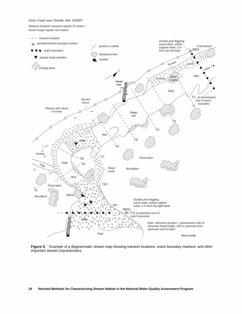
24 Revised Methods for Characterizing Stream Habitat in the National Water-Quality Assessment Program
Figure 5. Example of a diagrammatic stream map showing transect locations, reach boundary markers, and other important stream characteristics.
v vv
v vv
v vv
v vv
v vv
v vv
vv v
vv v
vv v
vv v
vv
v
vv v
vv v
v vv
v v
vv v
vv v
vv v
v vv
v vv
v
vvv
vv
vv
v vv
vv v
vvv
v vv
v vv
vv
vv v
vvv v
vvv
v
v
vv
v
vv v
vv
vv
vv
vv
Transect location
gravel or cobble
deciduous tree
boulder
semipermanent boundary marker
reach boundary
aquatic biota samples
eroding bank
Cottonwood
Double pink flagging,wood stake, yellowcapped rebar, 2 mfrom top left bank BM1
T1 at downstream end of reach
boundaryT2
T3
T4
Flow
Pool
Pool
Run
Deeprun
Deadtree
Eroding
bank
Run
Run
T7
T9
T8
T6
T5Riffle
Riffle
T10
BM11Bar
T11 at upstream end ofreach boundary
Floodchute
Double pink flagging, wood stake, yellow capped rebar, 1 m from top right bank
Note: reference location = downstream side of Seminary Road bridge, 205 m upstream fromupstream end of reach
Willow
Flood plain
Grassy
Electricfence
Terrace
Pasture with about5 horses
Path
Woodland
Flood plain
Woodland
Silvermaple
Duck Creek near Oneida, Wis. 5/28/97
Distance between transects equals 15 metersReach length equals 150 meters
N
Not to scale
Pool

are
g
t 5). cts ff nd t he be
r-
y
g ge
od and g rds one
en e nd nt ect a nt,
ge
is en e
After establishing the lower reach boundary and determining the length between transects, the crew proceeds upstream, flags transect locations by using flagging tape or surveying flags (Do not leave surveying flags behind; cows like to eat them!), measures the length of each GCU, and maps the reach (fig. 5). (If the area of each type of GCU is needed for other habitat classifications, measure two to three wetted channel widths per GCU in addition to length to calculate the area of each GCU.) The length of a GCU is an important determinant of habitat diversity that can affect the type and amount of instream biota. The diagrammatic map of the reach (fig. 5) should show the approximate area and type of each GCU, and the locations of major habitat features, reach boundaries, reference locations, discharge measurements, transects, semipermanent markers, and the flood plain, bars, islands, and shelves.
At the top of the reach, the upper permanent boundary marker is established at the last transect location. Channel, bank, and riparian features of each transect are measured as the crew moves back downstream. For nonwadeable reaches, collection of these types of data requires (at a minimum) a boat, a rangefinder or other long-range distance measurer, a surveying scale or laser-level survey system, and a depth-finder. Edsall and others (1997) contains more information on techniques and equipment for collecting habitat data in large streams.
The reach water-surface gradient is calculated by measuring the change in elevation of the water surface along the known length of the reach (distance from the upstream reach boundary to the downstream reach boundary). The water-surface gradient provides a good estimation of the energy gradient, which is an important parameter in the hydraulic power of the stream and, therefore, an important influence on a variety of other habitat measurements. The elevation change of the water surface can be determined by measuring the elevation of the left and(or) right edge of water directly or by measuring the water-surface elevation indirectly by recording the water depth and the elevation of the channel bed in the thalweg. If the latter method is used, two gradients can be calculated—one for the water surface and the other for the thalweg. In addition, the latter method may be more accurate in streams where the water’s edge is soft and the surveying rod could sink during the measurement. It may also be useful to measure the gradient of the
flood plain, which is the same as the water-surface gradient during bankfull flow.
Depending on the number of people in the sampling crew, the gradient measurements may be done while the transects are flagged and the GCU’s measured or during transect-data collection. The number of points used to measure the gradient alonthe reach and the type of equipment used varies, depending on the size and gradient of the stream. Usually, elevation data are collected at a spacing similar to the spacing between the 11 transects or aabout a distance of one channel width (Emmett, 197In high-gradient streams, the reach gradient can bedetermined by measuring the angle between transeby using a clinometer or compass and surveying starod, or by measuring the elevation change with a halevel and surveying staff rod (fig. 6). For low-gradienstreams, a hand level or clinometer may not provide taccuracy needed, in which case the gradient shoulddetermined with a surveying level on a tripod and a surveyor’s rod. For large, nonwadeable rivers, watesurface elevations are determined along one or bothbanks, and thalweg elevations can be determined buse of a hydroacoustic system.
For measuring gradient with a clinometer (fig. 6), the first step is to measure and flag the eye height of the person who is sighting on the surveyinrod. Next, the sighting person stands at the water’s edat one transect while the person with the surveying rmoves upstream or downstream to the next transect holds the survey rod at the water’s edge. The sightinperson sights to the mark on the survey rod and recothe angle between the transects. This procedure is dfor each set of transects.
For measuring gradient with a hand level or a surveyor’s level (fig. 6), differential leveling is done tomeasure the elevation drop and the distance betweselected transects along the reach. For example, thperson who is sighting stands between transect 1 atransect 2, and backsights (BS) to the semipermanemarker established at the reach boundary and trans1. This marker is considered a benchmark and has known or assumed elevation. From this measuremethe height of the instrument (HI) is obtained. Next, sightings are done to the rod placed at the water’s edat both transects and at a turning point (TP). These readings are called foresights (FS), or readings obtained from an unknown elevation. A turning point a temporary reference point, such as a rock or woodstake. As mentioned previously, instead of placing th
Collection of General Reach Data and Placement of Transects 25

es
am
od n
be
ll
d e
ly
Figure 6. Diagram of how to measure water-surface gradient with a clinometer or surveyor’s level.
Transect 1
Reach gradient = (h1 - h2) / L = tan (in degrees) (h1 - h2) = vertical elevation drop between transects L = distance between transects
BM
BS
BS
FS4FS1
FS3
TP
FS2
Transect 2Setup 1
Setup 2
Transect 3
θ
θ
Transect 2Transect 1 Transect 3
Clinometer
Surveyor's level (or hand level)
θ
Water surface
Water surface
h1h2
h3
L
BM = benchmarkTP = temporary turning pointBS = backsightFS = foresight
rod at the water’s edge, the rod also can be placed at the thalweg and a water-depth reading recorded. With this information, both the water-surface gradient and thalweg gradient can be calculated. After the foresights are done at both transects, the person who is sighting moves to a new location between transect 2 and transect 3. A backsight is taken from the rod at the turning point to establish the new height of instrument, and foresights are made to additional transects. This process is continued until the elevation drop along the entire reach has been measured. See Harrelson and others (1994) for more details.
Identification of Banks and Bankfull Stage
Several reach measurements require an understanding of some basic geomorphic concepts and definitions because the measurements are based on identifying the boundary between the flood plain, bank, and channel. The boundaries between these features are important because they are morphological indicators
that can be associated with flood and sediment characteristics. The first step in defining the boundaribetween flood plain, bank, and channel is to have aclear definition of each geomorphic feature.
The flood plain (fig. 7) is generally a flat to gently sloping depositional surface adjacent to a strechannel and is under construction by the modern stream. The surface of and the sediment under the floplain relate to the activity of the present river (Wolmaand Leopold, 1957). The elevation of this "active" flood plain under construction is considered here to the same as bankfull stage, as originally defined by Wolman and Leopold (1957). The change in the bankfull stage along the reach (flood-plain gradient)represents the water-surface gradient during bankfuflow. The flood plain is subject to periodic flooding approximately every 1 to 3 years (Wolman and Leopold, 1957; Wolman and Miller, 1960; Leopold anothers, 1964), although considerable variability in threcurrence interval of floods has been found amongdifferent streams (Williams, 1978). It is important to note that not all streams have flood plains, especial
26 Revised Methods for Characterizing Stream Habitat in the National Water-Quality Assessment Program
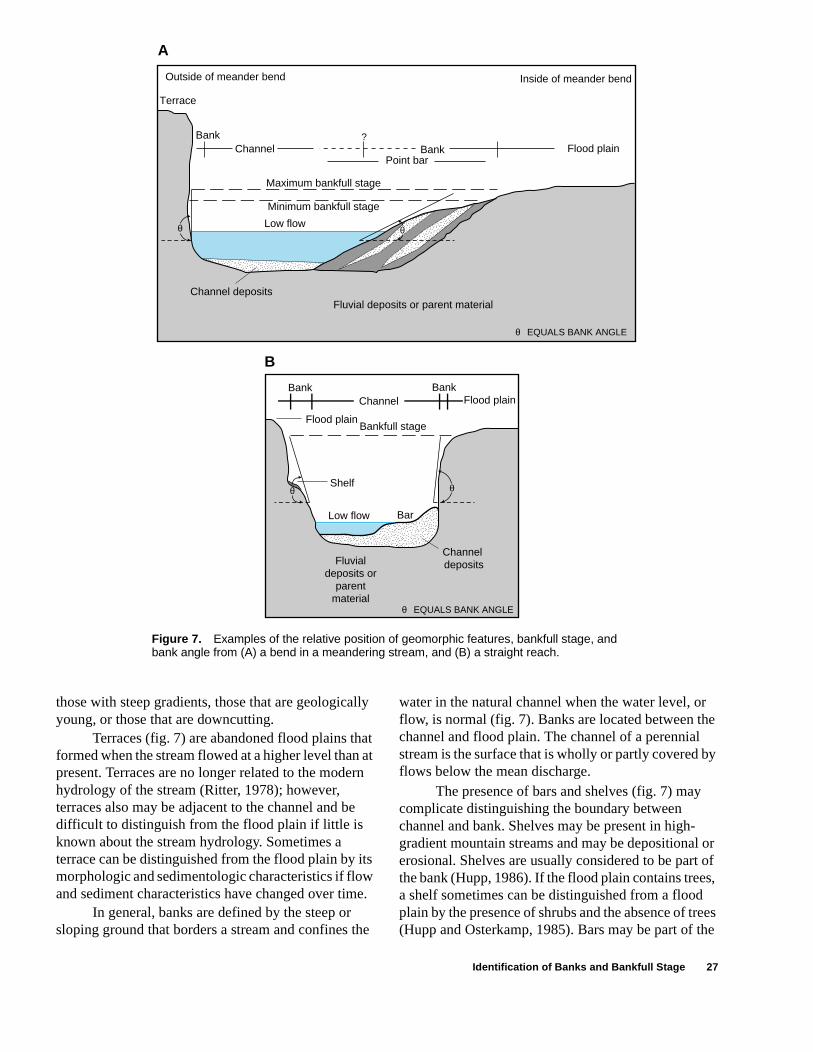
Figure 7. Examples of the relative position of geomorphic features, bankfull stage, and bank angle from (A) a bend in a meandering stream, and (B) a straight reach.
����yyyy
������yyyyyy
������yyyyyy
Terrace
Outside of meander bend Inside of meander bend
���������
yyyyyyyyyMinimum bankfull stage
Maximum bankfull stage
Low flow
Flood plainPoint bar
Channel Bank
Bankfull stage
Low flow
Flood plainChannelBank
Flood plain
Bank
Channel depositsFluvial deposits or parent material
Fluvialdeposits or
parentmaterial
A
B
Bar
?
Bank
Shelf
θθ
θ θ
Channel deposits
θ EQUALS BANK ANGLE
θ EQUALS BANK ANGLE
those with steep gradients, those that are geologically young, or those that are downcutting.
Terraces (fig. 7) are abandoned flood plains that formed when the stream flowed at a higher level than at present. Terraces are no longer related to the modern hydrology of the stream (Ritter, 1978); however, terraces also may be adjacent to the channel and be difficult to distinguish from the flood plain if little is known about the stream hydrology. Sometimes a terrace can be distinguished from the flood plain by its morphologic and sedimentologic characteristics if flow and sediment characteristics have changed over time.
In general, banks are defined by the steep or sloping ground that borders a stream and confines the
water in the natural channel when the water level, or flow, is normal (fig. 7). Banks are located between the channel and flood plain. The channel of a perennial stream is the surface that is wholly or partly covered by flows below the mean discharge.
The presence of bars and shelves (fig. 7) may complicate distinguishing the boundary between channel and bank. Shelves may be present in high-gradient mountain streams and may be depositional or erosional. Shelves are usually considered to be part of the bank (Hupp, 1986). If the flood plain contains trees, a shelf sometimes can be distinguished from a flood plain by the presence of shrubs and the absence of trees (Hupp and Osterkamp, 1985). Bars may be part of the
Identification of Banks and Bankfull Stage 27
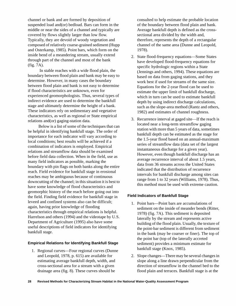
n -
r ,
s
are
rs,
is
es or m st
n ,
n , .
er,
f t f
s in e e e
channel or bank and are formed by deposition of suspended load and(or) bedload. Bars can form in the middle or near the sides of a channel and typically are covered by flows slightly larger than low flow. Typically, they are devoid of woody vegetation and composed of relatively coarse-grained sediment (Hupp and Osterkamp, 1985). Point bars, which form on the inside bend of a meandering stream, usually extend through part of the channel and most of the bank (fig. 7A).
In stable reaches with a wide flood plain, the boundary between flood plain and bank may be easy to determine. However, in many cases the boundary between flood plain and bank is not easy to determine if flood characteristics are unknown, even for experienced geomorphologists. Thus, several types of indirect evidence are used to determine the bankfull stage and ultimately determine the height of a bank. These indicators rely on sedimentary and vegetative characteristics, as well as regional or State empirical relations and(or) gaging-station data.
Below is a list of some of the techniques that can be helpful in identifying bankfull stage. The order of importance for each indicator will vary according to local conditions; best results will be achieved if a combination of indicators is employed. Empirical relations and streamflow data should be examined before field data collection. When in the field, use as many field indicators as possible, marking the boundary with pin flags on both banks along the entire reach. Field evidence for bankfull stage in erosional reaches may be ambiguous because of continuous downcutting of the channel; in this situation it is best to have some knowledge of flood characteristics and geomorphic history of the reach before going out into the field. Finding field evidence for bankfull stage in leveed and confined systems also can be difficult; again, having prior knowledge of flooding characteristics through empirical relations is helpful. Harrelson and others (1994) and the videotape by U.S. Department of Agriculture (1995) also have some useful descriptions of field indicators for identifying bankfull stage.
Empirical Relations for Identifying Bankfull Stage
1. Regional curves—Four regional curves (Dunne and Leopold, 1978, p. 615) are available for estimating average bankfull depth, width, and cross-sectional area for a stream with a given drainage area (fig. 8). These curves should be
consulted to help estimate the probable locatioof the boundary between flood plain and bank.Average bankfull depth is defined as the crosssectional area divided by the width and, therefore, represents the depth of a rectangulachannel of the same area (Dunne and Leopold1978).
2. State flood-frequency equations—Some Statehave developed flood-frequency equations for specific hydrologic regions within a State (Jennings and others, 1994). These equations based on data from gaging stations, and they work best if used for streams of the same size.Equations for the 2-year flood can be used to estimate the upper limit of bankfull discharge, which in turn can be used to estimate bankfull depth by using indirect discharge calculations, such as the slope-area method (Rantz and othe1982) and estimates of channel roughness.
3. Recurrence interval at gaged site—If the reachlocated near a long-term streamflow gaging station with more than 5 years of data, sometimbankfull depth can be estimated as the stage fthe 1.5-year flood based on an annual-maximuseries of streamflow data (data set of the largeinstantaneous discharge for a given year). However, even though bankfull discharge has aaverage recurrence interval of about 1.5 yearsdata from 36 streams across the United Statesindicated that the distribution of recurrence intervals for bankfull discharge among sites carange from 1 to 32 years (Williams, 1978). Thusthis method must be used with extreme caution
Field Indicators of Bankfull Stage
1. Point bars—Point bars are accumulations of sediment on the inside of meander bends (Ritt1978) (fig. 7A). This sediment is deposited laterally by the stream and represents active building of the flood plain. Usually, the texture othe point-bar sediment is different from sedimenin the bank (may be coarser or finer). The top othe point bar (top of the laterally accreted sediment) provides a minimum estimate for bankfull stage (Knox, 1985).
2. Slope changes—There may be several changeslope along a line drawn perpendicular from thdirection of streamflow in the channel bed to thflood plain and terraces. Bankfull stage is at th
28 Revised Methods for Characterizing Stream Habitat in the National Water-Quality Assessment Program
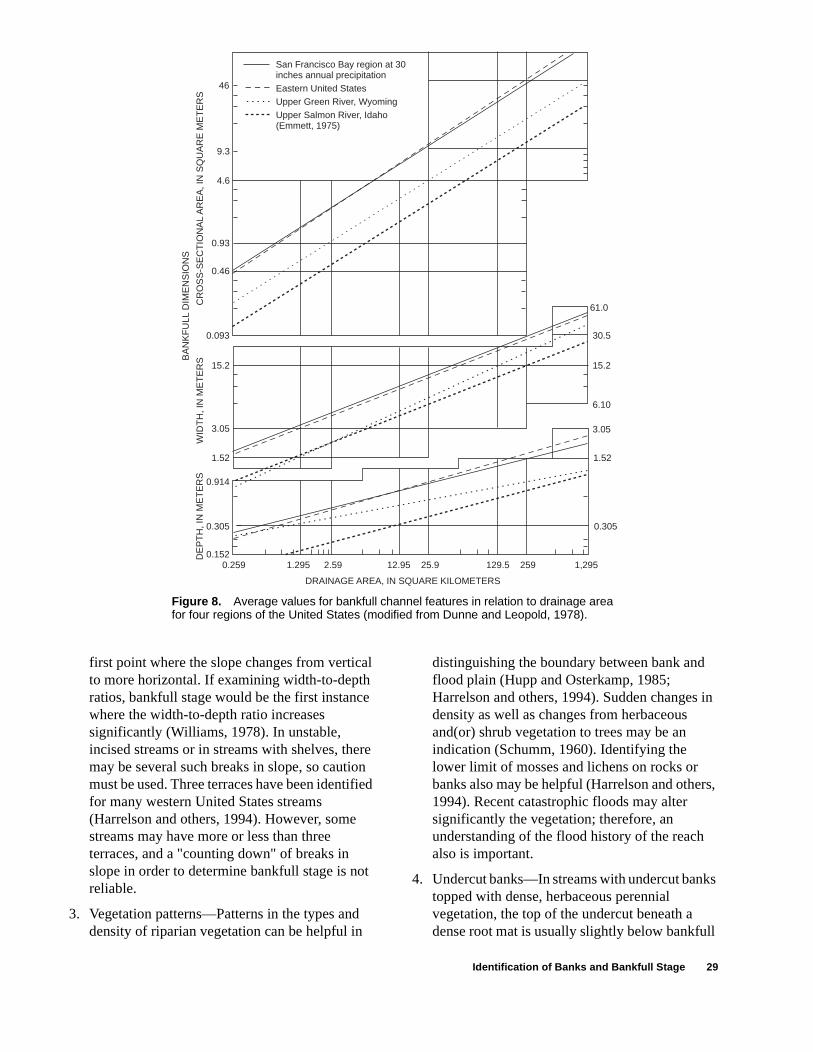
46
9.3
4.6
0.93
0.46
15.2 15.2
30.5
61.0
3.05 3.05
6.10
1.52 1.52
0.914
0.305 0.305
0.1520.259 1.295 2.59 12.95
DRAINAGE AREA, IN SQUARE KILOMETERS
25.9 129.5 259 1,295
0.093
DE
PT
H, I
N M
ET
ER
SW
IDT
H, I
N M
ET
ER
SBA
NK
FU
LL D
IME
NS
ION
S
CR
OS
S-S
EC
TIO
NA
L A
RE
A, I
N S
QU
AR
E M
ET
ER
S
San Francisco Bay region at 30 inches annual precipitationEastern United StatesUpper Green River, WyomingUpper Salmon River, Idaho(Emmett, 1975)
in
rs,
ks
ll
Figure 8. Average values for bankfull channel features in relation to drainage area for four regions of the United States (modified from Dunne and Leopold, 1978).
first point where the slope changes from vertical to more horizontal. If examining width-to-depth ratios, bankfull stage would be the first instance where the width-to-depth ratio increases significantly (Williams, 1978). In unstable, incised streams or in streams with shelves, there may be several such breaks in slope, so caution must be used. Three terraces have been identified for many western United States streams (Harrelson and others, 1994). However, some streams may have more or less than three terraces, and a "counting down" of breaks in slope in order to determine bankfull stage is not reliable.
3. Vegetation patterns—Patterns in the types and density of riparian vegetation can be helpful in
distinguishing the boundary between bank andflood plain (Hupp and Osterkamp, 1985; Harrelson and others, 1994). Sudden changesdensity as well as changes from herbaceous and(or) shrub vegetation to trees may be an indication (Schumm, 1960). Identifying the lower limit of mosses and lichens on rocks or banks also may be helpful (Harrelson and othe1994). Recent catastrophic floods may alter significantly the vegetation; therefore, an understanding of the flood history of the reach also is important.
4. Undercut banks—In streams with undercut bantopped with dense, herbaceous perennial vegetation, the top of the undercut beneath a dense root mat is usually slightly below bankfu
Identification of Banks and Bankfull Stage 29

f
nd n
, re, tts
nt d
tat.
ct
ed
e by
lly
stage (Harrelson and others, 1994). This method is best used as a last resort in steep channels lacking flood plains.
Collection of Transect Data
Transect data consist of quantitative information about channel width, bank features, water depth, velocity, substrate, habitat features, and riparian vegetation. Techniques for collecting transect data are different for wadeable and nonwadeable streams.
The first task in a wadeable stream is to extend a measuring tape perpendicular to the channel at a transect from the left bank to the right bank (the left side of a stream is usually considered "0"). The wetted channel width and bankfull channel width are measured, and the width of any channel features (bars, shelves, or islands) intersected by the tape are measured. The wetted channel width, along with depth, is used for estimating the water surface area and volume at low flow, which are useful for determining fish density or standing crop. The bankfull channel width is independent from streamflow conditions and is useful for determining the channel shape and the size of small frequent floods (floods with a recurrence interval of about 1.5 years). The bankfull channel width and bankfull depth (bank height) also are related to the size and type of transported sediment and the channel bed and bank substrate.
Two types of measurements for riparian vegetation near the stream are made—open canopyangle and riparian canopy closure. These measurements provide an estimate of the amount oshading in a reach, an important habitat feature for many fish, invertebrate, and algal species (Gorman aKarr, 1978; Byl and Carney, 1996). Riparian vegetatioinfluences the amount of sunlight entering a streamwhich controls photosynthesis and stream temperatuand also can affect streamflow and bank erosion (Plaand others, 1987). In addition to its influence on shading and temperature, riparian areas are importasources of organic material for aquatic organisms ancan help create and maintain complex instream habiRiparian areas also can act as important buffers between upslope land use and the stream.
The amount of open canopy is determined by standing at the center of the channel at each transeand measuring the right and left canopy angle with aclinometer or compass (fig. 9). The angle is measurfrom mid-channel to the tallest object on each bank.The right and left angles are subtracted from 180 degrees to give the open canopy angle, which can bconverted to percentage of open canopy by dividing 180 and multiplying by 100. The distance from the water surface to eye level should be noted, especiafor very narrow streams where canopy angle can begrossly underestimated by recording the angle fromeye level.
30 Revised Methods for Characterizing Stream Habitat in the National Water-Quality Assessment Program
Figure 9. Measurement of open canopy angle (modified from Platts and others, 1983).
Open canopy anglein degrees
Rightcanopyangle
Visiblehorizon
Leftcanopyangle
Stream
Eyelevel

’s
ve
ow e
rs, de
Riparian canopy closure is measured with a concave spherical densiometer by use of techniques outlined in Platts and others (1987). Measurement of canopy closure (the area of sky bracketed by vegetation) is preferred over measurement of canopy density (the area of sky blocked within the closure by vegetation) because measurements of canopy closure are less affected by seasonality than canopy density (Strichler, 1959). The densiometer is modified by taping a "V" on the mirrored surface (fig. 10). This modification uses only 17 of the possible 37 line intersections (points) and helps eliminate bias introduced by the overlap of vegetation reflected in the concave mirror when more than one reading is taken at the same position. At transects with woody vegetation
in wadeable streams, riparian canopy closure is measured with a spherical densiometer at the wateredge along both sides of the stream. At the water’s edge, the densiometer is held on the transect line perpendicular to the bank 30 cm from and 30 cm abothe shoreline. The number of line intersections surrounded by vegetation are counted for canopy closure (fig. 10).
For consistency and repeatability of measurements, it is extremely important to maintainthe same position for densiometer measures. This lposition accounts for vegetation most directly over thbanks and also incorporates any low overhead vegetation that overhangs the water (Platts and othe1987). Thus, a total of two readings (34 points) is ma
Collection of Transect Data 31
Figure 10. A concave spherical densiometer with bubble level, tape, and 17 points of observation. Line of intersections at both open and closed circles are examined. Closed circles represent line intersections counted in measurement of canopy closure (11 out of 17 points).
tape
vegetation
spherical densiometer
bubble leveled
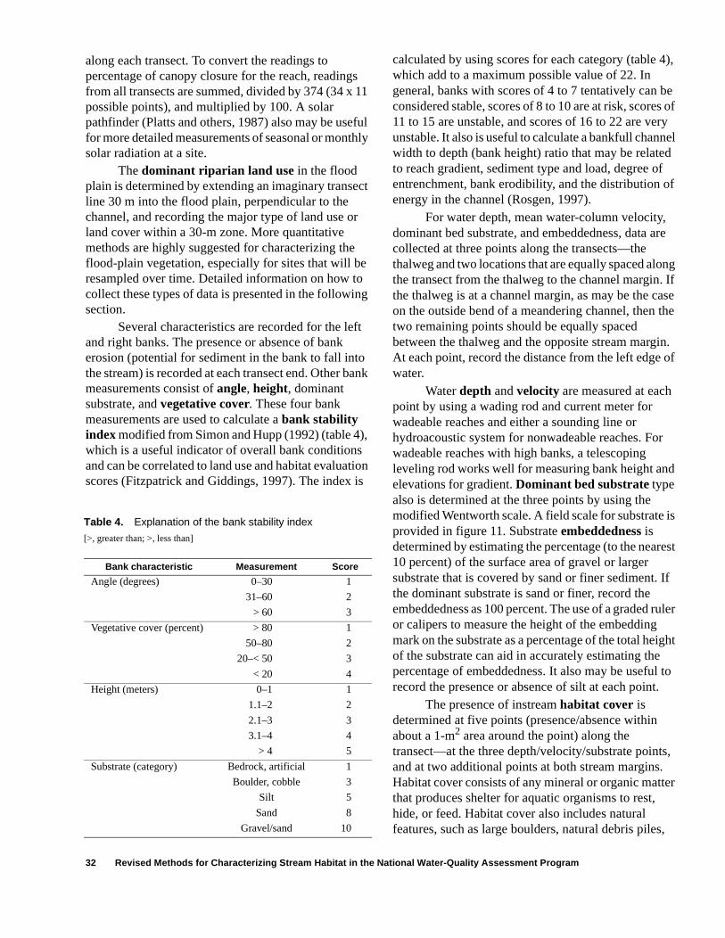
ng If ase the
in. of
r
d
along each transect. To convert the readings to percentage of canopy closure for the reach, readings from all transects are summed, divided by 374 (34 x 11 possible points), and multiplied by 100. A solar pathfinder (Platts and others, 1987) also may be useful for more detailed measurements of seasonal or monthly solar radiation at a site.
The dominant riparian land use in the flood plain is determined by extending an imaginary transect line 30 m into the flood plain, perpendicular to the channel, and recording the major type of land use or land cover within a 30-m zone. More quantitative methods are highly suggested for characterizing the flood-plain vegetation, especially for sites that will be resampled over time. Detailed information on how to collect these types of data is presented in the following section.
Several characteristics are recorded for the left and right banks. The presence or absence of bank erosion (potential for sediment in the bank to fall into the stream) is recorded at each transect end. Other bank measurements consist of angle, height, dominant substrate, and vegetative cover. These four bank measurements are used to calculate a bank stability index modified from Simon and Hupp (1992) (table 4), which is a useful indicator of overall bank conditions and can be correlated to land use and habitat evaluation scores (Fitzpatrick and Giddings, 1997). The index is
32 Revised Methods for Characterizing Stream Habitat in the N
is
rest
If
ruler
ight l to .
s, er
,
Table 4. Explanation of the bank stability index
[>, greater than; >, less than]
Bank characteristic Measurement Score
Angle (degrees) 0–30 1
31–60 2
> 60 3
Vegetative cover (percent) > 80 1
50–80 2
20–< 50 3
< 20 4
Height (meters) 0–1 1
1.1–2 2
2.1–3 3
3.1–4 4
> 4 5
Substrate (category) Bedrock, artificial 1
Boulder, cobble 3
Silt 5
Sand 8
Gravel/sand 10
calculated by using scores for each category (table 4), which add to a maximum possible value of 22. In general, banks with scores of 4 to 7 tentatively can be considered stable, scores of 8 to 10 are at risk, scores of 11 to 15 are unstable, and scores of 16 to 22 are very unstable. It also is useful to calculate a bankfull channel width to depth (bank height) ratio that may be related to reach gradient, sediment type and load, degree of entrenchment, bank erodibility, and the distribution of energy in the channel (Rosgen, 1997).
For water depth, mean water-column velocity, dominant bed substrate, and embeddedness, data are collected at three points along the transects—the thalweg and two locations that are equally spaced alothe transect from the thalweg to the channel margin.the thalweg is at a channel margin, as may be the con the outside bend of a meandering channel, then two remaining points should be equally spaced between the thalweg and the opposite stream margAt each point, record the distance from the left edgewater.
Water depth and velocity are measured at eachpoint by using a wading rod and current meter for wadeable reaches and either a sounding line or hydroacoustic system for nonwadeable reaches. Fowadeable reaches with high banks, a telescoping leveling rod works well for measuring bank height anelevations for gradient. Dominant bed substrate type also is determined at the three points by using the modified Wentworth scale. A field scale for substrateprovided in figure 11. Substrate embeddedness is determined by estimating the percentage (to the nea10 percent) of the surface area of gravel or larger substrate that is covered by sand or finer sediment.the dominant substrate is sand or finer, record the embeddedness as 100 percent. The use of a graded or calipers to measure the height of the embedding mark on the substrate as a percentage of the total heof the substrate can aid in accurately estimating thepercentage of embeddedness. It also may be usefurecord the presence or absence of silt at each point
The presence of instream habitat cover is determined at five points (presence/absence within about a 1-m2 area around the point) along the transect—at the three depth/velocity/substrate pointand at two additional points at both stream margins.Habitat cover consists of any mineral or organic mattthat produces shelter for aquatic organisms to rest, hide, or feed. Habitat cover also includes natural features, such as large boulders, natural debris piles
ational Water-Quality Assessment Program

Figure 11. Field scale for identifying particle-size classes from sand to small cobble.
(7) Small cobble > 64–128 millimeters
(6) Very coarse gravel > 32–64 millimeters
(5) Coarse gravel > 16–32 millimeters
(4) Fine to medium gravel > 2–16 millimeters
(3) Sand > 0.063–2 millimeters
2 16 32 64 128
(4) Number refers to substrate category number
undercut banks, aquatic macrophyte beds, and overhanging vegetation, as well as structures such as discarded tires, appliances, and automobile parts. All habitat-cover categories present at each 1-m2 point are recorded. The abundance of each type of habitat cover (in percent) is calculated from the 55 possible measurements for the 11 transects (5 points per transect).
For large, nonwadeable streams, transects are established as for wadeable streams. However, data cannot be collected along the transects in the same fashion as in wadeable streams. In nonwadeable streams, a paper-trace hydroacoustic system is attached to a boat, and the boat is moved along the transect. The depth finder produces a depth profile of the stream along the transect. From the paper printout of the depth finder, three measures of depth are made, corresponding to the three points along the transect as measured in wadeable streams. Samples of bottom substrate may be collected at each point with a sediment coring device, a Ponar sampler, or an Ekman dredge. However, collection of bottom substrate may be impossible on many large rivers. Habitat cover data are collected only at 22 points along the shoreline. For NAWQA national data-aggregation requirements, Study Unit personnel should attempt to collect depth, width, riparian canopy closure, canopy angle, and habitat cover at nonwadeable sites, if possible.
Bottom substrate, embeddedness, and velocity data are not required at nonwadeable sites. Individual Study Units may desire to collect additional information on bottom substrate, velocity, and habitat features in nonwadeable streams. Collection of habitat characteristics from large rivers should reflect the most important features that are thought to be affecting biota sampled at a site. A variety of equipment has been used
in such streams, including side-scan sonar, acoustic doppler current profilers, and remotely operated underwater camera systems. Edsall and others (1997) provide information on the applicability and use of these kinds of equipment in large rivers. Aerial videography is a relatively inexpensive, easy-to-use alternative to other remote sensing techniques for measuring macrohabitat features in streams greater than 15-m wide (Jennings and others, 1994; Seibert and others, 1996).
Additional Optional Measurements
Depending on Study Unit goals, it may be useful to collect additional information on channel stability, riparian vegetation, and bottom- and bank-substrate characteristics, especially if there is the potential for changes in habitat caused by changes in land use, hydrology, or sediment input. If collected, these data can be stored in the habitat data dictionary files called "Chansect" for cross sections, "Veg" for riparian vegetation data, and "Substrat" for bottom- and bank-substrate quantification. In the original habitat protocol (Meador, Hupp, and others, 1993), channel cross sections and point-quarter riparian vegetation were elements required for national data aggregation. Elements of the channel cross-section survey, such as reach gradient, have been separated from the overall channel cross-section effort; only these selected elements are listed as required in the present document. Evaluation of point-quarter sampling techniques has suggested that the methods may not be applicable nationally. Thus, the point-quarter vegetation sampling was changed from a required to an optional measurement. While densiometer measures are not
Additional Optional Measurements 33
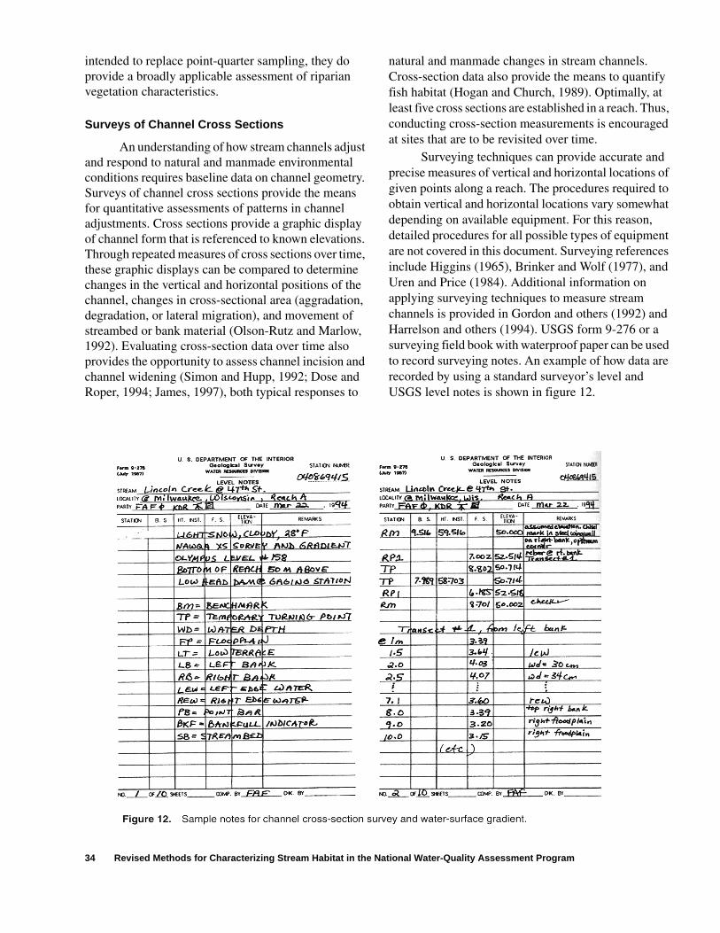
intended to replace point-quarter sampling, they do provide a broadly applicable assessment of riparian vegetation characteristics.
Surveys of Channel Cross Sections
An understanding of how stream channels adjust and respond to natural and manmade environmental conditions requires baseline data on channel geometry. Surveys of channel cross sections provide the means for quantitative assessments of patterns in channel adjustments. Cross sections provide a graphic display of channel form that is referenced to known elevations. Through repeated measures of cross sections over time, these graphic displays can be compared to determine changes in the vertical and horizontal positions of the channel, changes in cross-sectional area (aggradation, degradation, or lateral migration), and movement of streambed or bank material (Olson-Rutz and Marlow, 1992). Evaluating cross-section data over time also provides the opportunity to assess channel incision and channel widening (Simon and Hupp, 1992; Dose and Roper, 1994; James, 1997), both typical responses to
natural and manmade changes in stream channels. Cross-section data also provide the means to quantify fish habitat (Hogan and Church, 1989). Optimally, at least five cross sections are established in a reach. Thus, conducting cross-section measurements is encouraged at sites that are to be revisited over time.
Surveying techniques can provide accurate and precise measures of vertical and horizontal locations of given points along a reach. The procedures required to obtain vertical and horizontal locations vary somewhat depending on available equipment. For this reason, detailed procedures for all possible types of equipment are not covered in this document. Surveying references include Higgins (1965), Brinker and Wolf (1977), and Uren and Price (1984). Additional information on applying surveying techniques to measure stream channels is provided in Gordon and others (1992) and Harrelson and others (1994). USGS form 9-276 or a surveying field book with waterproof paper can be used to record surveying notes. An example of how data are recorded by using a standard surveyor’s level and USGS level notes is shown in figure 12.
34 Revised Methods for Characterizing Stream Habitat in the National Water-Quality Assessment Program

To determine profiles of channel cross sections, five transects that best represent the geomorphic features of the reach should be selected. Two of the cross sections should be located at the reach boundaries, one at the upstream end and one at the downstream end. Endpoints of each cross section should be above bankfull height; it is preferable to have at least two or more points in the flood plain or on higher surfaces. Permanent markers and elevation benchmarks for one or both endpoints of the cross section should be established. Details for establishing elevation benchmarks and permanent markers are provided in Harrelson and others (1994). Benchmarks should be referenced to known elevation points. In some cases, known elevations can be the elevation benchmarks of a USGS gaging station, a bridge, a nearby highway, or a benchmark for recent urban development. It is very helpful to establish this information before going into the field. Local surveying firms may provide additional useful information.
To define the cross-section profile, the left endpoint is measured first, and bed elevations at each change in an important feature are measured, including the edge of water, the water surface, and the channel bed (fig. 13). The left side of the channel is determined when facing downstream. In general, the spacing of
elevation measurements along the transect is determined by the shape of the channel; however, elevation measurements should be done at every point where the slope changes. If the surface is flat, elevations should be determined about every 0.5 m or at regular intervals equal to the channel width divided by 20 (Harrelson and others, 1994). Elevations at isolated features, such as boulders or logs, are avoided. As elevations are taken from left to right, the horizontal distance between endpoints and water-depth measurements also is recorded. The survey must be closed by taking a reading back to the elevation benchmark.
Riparian-Vegetation Characterization
Densiometer measurements provide quantitative information on overhead canopy closure above the channel and along channel margins; however, they do not provide information on the density, dominance, and species of woody vegetation in the riparian zone. Woody vegetation in the riparian zone may directly influence channel conditions, water chemistry, the amount of large woody debris, and aquatic communities in the reach (Lowrance and others, 1984; Gurtz and others, 1988; Sweeney, 1993; Large and Petts, 1994; Trimble, 1997) and, in turn, may be affected by flooding characteristics and the presence of
Additional Optional Measurements 35
Figure 13. Example of measurement points for cross-section profiles.
TERRACE
FLOOD PLAIN
Left edge ofwater Right edge
of water
Water depth measurement takenalong with channel-bottom
elevation measurement
STREAMELEVATION
MEASUREMENT

fluvial landforms (Hupp and Osterkamp, 1985, 1996; Johnson and others, 1995). For example, high densities of vegetation at one site compared to low densities of vegetation at another could be explained by a predominance of mature cypress trees at one site compared to a predominance of young red maples at the other. Because red maples are more likely to populate an area after disturbance, knowledge of species and basal area information may be very important to aid interpretation of differences in conditions among sites (Simon and Hupp, 1992).
The point-centered quarter method (Mueller-Dombois and Ellenberg, 1974) provides quantitative estimates of stem density and basal area (biomass), and a permanent record of the woody species supported by the riparian zone. For the point-centered quarter method, sampling points usually are established at a point in the flood plain along a transect that is most representative of the dominant woody vegetation that has the most influence on channel conditions. This
point is usually located in the flood plain but also may be along the bank in entrenched streams with little or no flood plain or along braided streams that have wide banks. A minimum of 10 points is measured along the reach, selecting among the most representative of the 22 possible points at the ends of the 11 transects. The same geomorphic surface (flood plain or bank) should be sampled for all points. At each point, four quarters are established, formed by the intersection of two perpendicular lines, one of which is the transect line (fig. 14). Trees and shrubs are included in the measurement if they are at least breast height (1.5 m). Trees are distinguished from shrubs in that trees are at least 2 m high and have a diameter at breast height (dbh) of at least 3 cm. The sampled trees or shrubs are identified to species, and the distance from the sampling point to the nearest tree or shrub in each quarter is measured, along with the dbh (fig. 14). Measurement of the same tree twice should be avoided, otherwise it may cause over-representation of certain
36 Revised Methods for Characterizing Stream Habitat in the National Water-Quality Assessment Program
Figure 14. Point-centered quarter method used to evaluate density and dominance of bank woody vegetation.
Tree orshrub
Quadrant1
Quadrant2
Quadrant3
Quadrant4
Sampling point
Transect line
Second line
Stream
Measured distanceto closest tree or shrub in quadrant
species. Where bank woody vegetation is growing in narrow strips or rows, the two closest trees or shrubs on either side of the sampling point (a total of four trees or shrubs) are measured. In open sites with a potential for less than four trees or shrubs per point, the quarter-point method should not be used. Where a single tree or shrub has developed many separate trunks, an average dbh for three trunks is recorded, along with the total number of trunks. (The average dbh is multiplied by the number of trunks to calculate total basal area and biomass.) Measurements are recorded in a field notebook. Pertinent information to record includes transect number, left or right side of channel, geomorphic surface (flood plain, bank, bar), species, distance to species (in meters), dbh, and number of trunks. It also is important to record local conditions that prevent quarter-point measurements, such as a clearcut or pasture. To record the species, use a four-letter code based on the first two letters of the scientific name for the genus and the first two letters of the species (for example, "BENI" is recorded for Betula nigra).
Stem density of all woody species combined is calculated by dividing a unit area by the square of the mean point-to-tree distance. Unit area refers to the size of the area, in the same units as those for the mean area per tree, on the basis of which density is to be expressed. Typically, 100 m2 is chosen as the unit area. Several steps are required to calculate stem density for all woody species:
1. Calculate a total for all point-to-tree distances per reach.
2. Calculate the mean point-to-tree distance per reach.
3. Calculate the square of the mean point-to-tree distance per reach. (This value gives the mean area per plant, representing the average area of ground surface on which one plant occurs.)
4. Divide the unit area (100 m2) by mean point-to-tree distance per reach squared.
To determine the mean basal area for all woody species combined, calculate the basal area for each tree using the following formula:
(1)
or Area = 0.7854 (dbh)2. A mean basal area can then be determined for the entire reach.
Permanent vegetation plots are established to document trends in riparian vegetation over time. Plots are established where stability or change in the riparian vegetation is particularly important for water-quality analyses. For example, it may be useful to establish plots along urbanizing reaches, forested streams with the potential for logging, or reference sites. To construct a permanent vegetation plot, an area at the end of each surveyed cross section is selected. A 20- by 20-m plot is identified by using a tape measure for distance and a compass to establish 90-degree angles at the corners of the plot. The corners are marked with semipermanent boundary markers. The edge of the plot nearest the bank should be at least several meters from the bank. Sample the vegetation by determining the diameter and species of all trees and shrubs within the plot. Record only living trees and shrubs. If the riparian zone is narrow such that a 20- by 20-m plot cannot be established, then two or more smaller plots are established so that the total area sampled equals 400 m2. Where herbaceous vegetation is clearly dominant, then a 10- by 10-m square plot is established. At herbaceous vegetation plots, the aerial coverage of up to five species is measured, and the percentage of these species within the plot is calculated. Vegetation plots are usually established at the ends of surveyed cross sections.
Substrate Characterization
Quantitative measurement of channel-substrate particle size can be made by means of Wolman pebble counts (Wolman, 1954) in wadeable reaches where substrates are coarse or by the collection of sediment for laboratory analysis where substrates are composed of sand or finer material. Both types of data provide a more quantitative measure of substrate characteristics than can be obtained through categorical observations. Quantitative data gathered from pebble counts are particularly useful for fish and invertebrate community analyses. A pebble count is done as follows:
1. Begin the count at each transect at bankfull elevation on the left bank and proceed to bankfull elevation on the right bank.
2. Proceed one step at a time, with each step constituting a sampling point.
3. At each step, reach down to the tip of your boot and, with your finger extended, pick up the first
Area π dbh( )2
4--------------------=
Additional Optional Measurements 37

pebble-size particle touched by the extended finger.
4. To reduce sampling bias, look across and not down at the channel bottom when taking steps or retrieving bed material.
5. As you retrieve each particle, measure the intermediate axis. If the intermediate axis cannot be determined easily, measure the long diameter and the short diameter of the particle, and determine the average of the two numbers. The transect may have to be traversed several times to measure 100 pebbles.
Thus, the size distribution of particles is determined and expressed in percentage by number of particles. A count of 100 particles is recommended; however, 50 or 25 particles can be measured.
To obtain a quantitative determination of fine-grained substrate, three samples of the bed material are collected along each transect and composited. In addition, samples of the bank-substrate material can be collected from one or both banks. These samples are returned to the laboratory for sieve analysis. Size fractions are determined by the Study Unit; however, at a minimum, analyses should be conducted for sand, silt, and clay fractions.
38
r
ce 62 manent the e location ges in
Description and List of Reach-Scale Habitat Characteristics
Detailed descriptions and lists are given below for collecting general reach information and transect data. Two example field forms for use at wadeable sites are shown in field forms 3 and 4 (see Field Forms at back of report). An example for recording reach gradient channel cross-section data on USGS level notes is shown in figure 12. Optional information on riparian vegetation (point-quarter and vegetation plots) and sediment characteristics (Wolman counts and sediment collection) should be recorded on waterproof paper in field note books.
General Reach Information
Detailed field methods for collecting general reach data are listed below. An example form is shown in field form 3. Items listed in bold are required for NAWQA national data aggregation. Abbreviations in parentheses are parameter codes for the NAWQA habitat data dictionary. These data are stored in files called "Reach" and "Gcu" in the habitat data dictionary.
1. Study Unit (SUID)—Use the 4-letter code designated for each Study Unit.
2. Station identification number (C001 or STAID)—List the USGS station identification numbefor the site.
3. Date (DATE)—Record the date as month, day, and year (4-digit year).
4. Reach (REACHSEQ)—Reach sequence letter, usually an "A." If more than one reach is characterized at the station, then assign sequential letters.
5. Station name (C900)—Record the USGS stream name.
6. Description of reference location (REFLOC)—Provide a general description of the referenlocation (for example, "gage on left bank just below Highway 1462 bridge" or "Highway 14bridge, upstream edge"). The reference location should be a permanent structure. If no perstructure is present, a semipermanent marker (such as an iron pipe) should be installed atlocation. The reference location provides the geographic link to habitat data collected at thsegment and basin scale. Photos of the reference location should be taken. If the reference is a bridge, a photograph of the reach from the bridge will be useful for documenting chanthe overall character of the reach over time.
Revised Methods for Characterizing Stream Habitat in the National Water-Quality Assessment Program

ta.
r
pling. n is t on a
recorder
ing be which s.
se
water nt is ts the mean or are not uding
w). If reach e
reams,
within etween
follow
tion If either
7. Investigators (INVEST)—Names of the investigators are useful if followup information is necessary. The team leader’s name is logged in the NAWQA habitat data dictionary.
8. Quality of habitat sampling effort (RCHQUAL)—This is used to denote the quality of the da
9. Comments on habitat sampling or conditions (REACHCOM)—Note the general conditions ofthe reach. Be sure to note factors, such as recent flood history, beaver activity, and weatheconditions.
10. Stage (STAGE)—Record water level as measured to a known point at the time of habitat samUsually, at fixed sites, this information will come from the gaging station. If no gaging statiopresent and data may be collected at the site more than once, measure from a known poinbridge or other permanent object. Be sure to note units of measure.
11. Stage method (STAGEMD)—The method used to measure stage, such as automatic data (ADR), staff, or tape-down.
12. Instantaneous discharge (DISCH)—If no gaging station is present, measure discharge by usUSGS techniques (Rantz and others, 1982). Use USGS form 9-275-F. Habitat data shouldcollected during stable low-flow conditions. This discharge measurement reflects base flow, is an important habitat feature (Johnson and others, 1995) and is useful for comparing site
13. Discharge method (DISCHMD)—Record method used for discharge measurement: gagingstation, wading rod, estimated (describe how), other.
14. Channel modification at reach (CHMOD)—Note any amount of channel modification at thereach. Choose from categories of concrete lined, stabilized, dredged, channelized but not stabilized, wing dams, lightly affected, or not modified. If only a small section is modified, u"lightly affected."
15. Mean channel width (MCW)—The wetted channel width is measured from the left edge of to the right edge of water along the existing water surface. This channel-width measuremeused for estimating the needed reach length. Select the appropriate location that represenaverage reach width. Make three measurements of wetted channel width and calculate thechannel width. To provide consistency in measurement, protruding logs, boulders, stumps,debris surrounded by water are included in the measurement of the water surface. Islandsincluded in the measurement. Any solid accumulation of inorganic sediment particles protrabove the water and supporting woody vegetation is considered an island.
16. Curvilinear reach length (REACHLEN)—The curvilinear reach length is measured by following the path of the thalweg (the part of the stream with the deepest water and most flothere is no distinct thalweg (a possibility in a run), then follow the center of the channel. The length is computed by multiplying the mean channel width by 20. For wadeable streams, thminimum and maximum reach lengths are 150 and 300 m, respectively; for nonwadeable stthe minimum and maximum reach lengths are 500 and 1,000 m, respectively.
17. Distance between transects (TRANDIS)—Eleven equidistant transects are spaced evenly the reach. The distance between transects is the reach length divided by 10. The distance btransects is measured by following the thalweg of the channel. If no thalweg is observable, the center of the channel.
18. Curvilinear distance from reference location to reach ends (USRCHEND and DSRCHEND)—Measure the curvilinear distance (follow the thalweg) from the reference locato the upstream and downstream reach boundaries by using a range finder or tape measure.
Description and List of Reach-Scale Habitat Characteristics 39

40
arker
ry e, "iron irection this
ilinear which veyor’s high-d to get wed ect or at the the asures t scale nsects e a lot s are istance
rate fferent e
ow. t of the ta on
50 ide r
of the ide e the
boundary is upstream from the reference location, its value is negative; otherwise, it is positive. This information will be used to locate the reach in the future.
19. Location of boundary markers (USBMBK, DSBMBK)—Note the location of the boundary markers to aid in locating them in the future. Record whether the semipermanent boundary mis on the left bank, the right bank, or both banks (looking downstream).
20. Boundary marker descriptions (USBMDESC, DSBMDESC)—Describe the type of boundamarker and measure the distance from the channel (top of bank or water’s edge) (for examplbar, painted orange, about 2 m from the wetted channel") and the distance and compass dto other landmarks that may help in locating the boundary marker in the future. A record ofinformation is key to finding the location of the reach in the future.
21. Reach water-surface gradient (RCHGRAD)—Reach water-surface gradient is the differencebetween the water-surface elevation at the top and bottom of the reach divided by the curvreach length. The water-surface gradient provides a good estimation of the energy gradient,is an important parameter in the hydraulic power of the stream and, therefore, an importantinfluence on a variety of other habitat measurements. This measurement is made with a surlevel for low-gradient streams, or can be estimated with a clinometer or Abney hand level forgradient streams (fig. 6). For a clinometer measurement, first mark a pole or use a stadia ro"eye height" of the person who is holding the clinometer. Flag this mark so that it can be viefrom a distance. Next, have each person stand at the water’s edge, preferably at each transobservable breaks in the water surface. Look through the clinometer with one eye and viewstaff or rod with the other, raising or lowering the clinometer until the cross hairs line up withcorrect mark on the pole or rod. Record the slope in dimensionless units. If the clinometer mepercentage, divide the values by 100 to get dimensionless units. Make sure you know whayou are using on the clinometer! The number of sightings also can be reduced by skipping traand moving to the farthest transect that can still be sighted effectively; however, there can bof variability in just a few measurements of water’s edge, so be sure enough measurementmade. For double-checking, it could be advantageous to take measurements at the same dalong both right and left edges of water. Also, some reaches may be too flat to get an accuestimation by using this technique. Note that the gradient of the channel bed may be very difrom the water surface; thus, one cannot be substituted for the other. Also, the water-surfacgradient at low flow will not always be the same as the water-surface gradient at bankfull flDepending on Study Unit goals, it may be useful to measure water-surface gradient, gradienchannel bed thalweg (THGRAD), and gradient at bankfull (flood-plain gradient). Record daUSGS field notes or in a field book. Use the reach field form (field form 3) to record final calculations of reach water-surface gradient.
22. Method used to measure reach gradient (RCHGRAMD)—Record the method used, such assurveying level, clinometer, hand level, or other.
23. Geomorphic channel units (GCUSEQ, GCUTYPE, GCULEN)—While mapping the reach, draw (see diagrammatic mapping) and record all riffles, runs, or pools that are greater thanpercent of the channel width, and measure and record the length of each. These data provinformation on spatial dominance and diversity of habitat types. See previous discussion foinformation about identifying GCU’s. Use additional space as needed.
24. Diagrammatic mapping (not in data dictionary)—Draw a schematic or representative map reach (see, for example, fig. 5). The mapping of all GCU’s and habitat features can provcritical information needed to evaluate temporal trends in habitat. The map should includ
Revised Methods for Characterizing Stream Habitat in the National Water-Quality Assessment Program

, orphic rawing
it for nsect,"
r
d year
elp in to
e ansect, s, and film at reduces ortant plicates The view
nd other rded.
islands
locations of GCU’s, habitat features, and bank and flood-plain land use and land cover to approximate scale. Include the reference location, bridges, road names, reach boundarieslocations of semipermanent boundary markers, and transect locations relative to the geomunits. Draw the approximate aspect of the reach. Include a north arrow and the direction ofstreamflow. For reference, paste an example map or explanation to the clipboard used for dthe maps.
Transect Information
An example transect form is shown in field form 4 (see Field Forms at back of report) for recording information for wadeable streams. One form is filled out for each transect. Items in bold are required for NAWQA national data aggregation. Other features listed are helpful to the Study Undocumenting long-term changes and revisiting the site. These data are stored in files called "Tra"Chfeat," "Habfeat," and "Tranpnt" in the habitat data dictionary.
1. Station identification number (C001 or STAID)—List the USGS station identification numbefor the site.
2. Reach (REACHSEQ)—Reach sequence letter, usually an "A." If more than one reach is characterized at the station, then assign sequential letters to additional reaches.
3. Date (DATE)—Record the beginning date of reach and transect sampling as month, day, an(4-digit year).
4. Transect number (TCTNO)—The sequential number of each transect is recorded (usually 1through 11) for each site.
5. Habitat type (HABTYPE)—Record whether the transect is located in a riffle, pool, or run. Sometimes it is useful to analyze features in each type of habitat, and this information will hgrouping transect information on the basis of habitat type. For example, it might be useful distinguish between substrate type in riffles and substrate type in pools.
6. Photodocumentation (not in data dictionary)—Note whether or not photos were taken at thtransect. Record the exposure number in the blank. Optimally, stream conditions at each trespecially those at the reach boundaries, are photographed. Photographs are taken facingupstream, perpendicular to the channel, and downstream, from either the left or right bankthey should include a scale reference. Color slide film is preferred. Use of the same type of all sites and at the same site over time increases comparability of repeat photographs and variability related to film development. The inclination and aspect of the camera lens are impand can be measured with a compass. A level camera is preferred because inclination comthe perspective of the view and makes accurate duplication of repeat photographs difficult.aspect of the camera can be noted by pointing a compass at the central aiming point in theand recording the compass reading. Camera lens size, camera type, exposure, film type, aappropriate documentation information for taking 35-mm color photographs should be recoSemipermanent markers can be established at these locations to facilitate taking repeat photographs.
7. Wetted channel width (CHWIDTH)—Measure the wetted-channel width along the transectfrom the left edge of the water to the right edge of the water. Do not include bars, shelves, or in width.
Description and List of Reach-Scale Habitat Characteristics 41
42
m useful
full
t of ank ody adient once a
0) rallel to
sible eam. ight of bank; is done d from d to angle + solar onal or
others over
tion f t with a th sides r to the ed by
. This etation
closure
8. Bankfull channel width (BFWIDTH)—Measure bankfull channel width along the transect frothe top edge of the left bank to the top edge of the right bank. See previous discussion for indicators of banks and bankfull stage.
9. Channel width method (CHWIDRM)—Record the method used to measure wetted and bankchannel width.
10. Channel features (CHFEAT, CFWIDTH)—If channel bars, shelves, or islands are present, measure width using a tape measure or rangefinder. Channel bars are the lowest prominengeomorphic feature higher than the channel bed (fig. 7). Channel bars are typically devoid woody vegetation and consist of relatively coarse sand, gravel, and cobbles. Shelves are bfeatures extending nearly horizontally from the flood plain to the lower limit of persistent wovegetation (Hupp and Osterkamp, 1985). Shelves are most common along relatively high-grstreams. Islands are mid-channel bars that have permanent woody vegetation, are floodedyear on average, and remain stable except during large flood events.
11. Aspect (CHANHEAD)—The aspect of the downstream flow is recorded in degrees (0 to 36using a compass. At the midpoint of the transect, face downstream and point a compass pastreamflow.
12. Canopy angles (LCANANG, RCANANG, CANANG)—Open canopy angle or sun angle is formed by the angles from midpoint of the transect (midpoint of the channel width) to the vihorizon at either bank. It is a measure of the amount of sunlight potentially reaching the strFrom the midpoint of the transect, use a clinometer to determine the angle from the line of sthe investigator to the tallest structure (for example, tree, shrub, building, or grass) on the leftthis is called the left canopy angle (in the general area of the transect). The same procedurefor the right bank (right canopy angle). The sum of these angles is computed and subtracte180 degrees. The result, the open canopy angle or sun angle (fig. 9), also can be convertepercentage of open canopy ((sun angle/180) x 100) or percentage of shade ((right canopy left canopy angle/180) x 100). On narrow streams, note the measurement at eye height. A pathfinder (Platts and others, 1987) may be useful for more detailed measurements of seasmonthly solar radiation at a site.
13. Riparian canopy closure (LBSHAD, RBSHAD, CANCLOSR)—Riparian canopy closure is measured with a concave spherical densiometer by use of techniques outlined in Platts and(1987). Measurement of canopy closure (the sky area that includes vegetation) is preferredmeasurement of canopy density (the sky area that is blocked by vegetation), because measurements of canopy closure are less affected by seasonality than canopy density. Thedensiometer is modified by taping a right angle on the mirror surface (fig. 10). This modificauses only 17 of the possible 37 points and helps eliminate bias introduced by the overlap ovegetation reflected in the concave mirror when readings are taken at the same position. Atransects with woody vegetation in wadeable streams, riparian canopy closure is measuredspherical densiometer at two positions along the transect—at the water’s edge and along boof the stream. At the water’s edge, the densiometer is held on the transect line perpendiculabank 30 cm from and 30 cm above the shoreline. The number of line intersections surroundvegetation are counted for canopy closure (fig. 10). For consistency and repeatability of measurements, it is extremely important to maintain the same position for the densiometerposition accounts for vegetation most directly over the banks and also incorporates any vegthat overhangs the water (important for fish habitat (Platts and others, 1987)). A total of tworeadings (34 points) is made per transect. To convert the readings to percentage of canopy
Revised Methods for Characterizing Stream Habitat in the National Water-Quality Assessment Program

(use a lain. ing a ach can ach at rs
ank or e or n the
d and
y y from ank
is may be ded. A
for the reach, readings from each transect are summed, divided by 374 (34 x 11), and multiplied by 100. If no woody vegetation is present, a value of "0" is recorded.
14. Dominant riparian land use/land cover (LBLULC, RBLULC)—At each transect, the dominant riparian land use is recorded for each bank within an approximate 30-m distancerangefinder or other method for approximating 30 m) from the top of the bank into the flood pOnly one land-use category should be recorded for each bank for each transect, representvisual band on either side of the transect. The percentage of each type of land use for the rebe estimated by summing the number of occurrences of each land use, dividing by 22 (2 e11 transects) and multiplying by 100. The categories are modified from Simonson and othe(1994a):
Agricultural:Cropland (annually harvested row crops, hay fields, or orchards) CRPasture (regularly grazed by livestock, wooded, or open) PAFarmstead/barnyard (feedlots, confined livestock areas, farm buildings) FMSilviculture (tree plantation or logged woodland) SI
Developed:Urban residential/commercial (houses, apartments, commercial UR buildings, parking lots)Urban industrial (industrial buildings and parking lots) UIRural residential (low-density housing development in a rural setting) RRRight-of-way (paved or unpaved roads, railroads, paved paths, RW powerlines)
Less disturbed:Grassland (grass/hedges not subject to regular mowing or grazing) GRShrubs or woodland (woody plants) SWWetland (covered by water much of the year; may be forested, shrubby, WE or open)Other (exposed rock, desert, and so on) OT
If the 30-m riparian zone is a slumped bank or bluff, record the land use at the top of the bbluff. For national consistency, a riparian distance of 30 m was selected to encompass thmajority of riparian conditions across a wide range of environmental settings. At the local regional scale, however, effects of riparian width on water quality are varied and depend otype of vegetation and geologic setting. The Study Unit may use additional methods to characterize riparian vegetation or human disturbance depending on Study Unit issues anenvironmental setting. Depending on Study Unit goals, more quantitative data on speciesdominance, frequency, and distribution can be collected through point-quarter techniquesvegetation plots (refer to discussion of point-quarter techniques for more details).
15. Bank angle (LBANGLE, RBANGLE)—A clinometer is used to measure the angle formed bthe downward-sloping bank as it meets the stream bottom. The angle is determined directla clinometer placed on top of a surveyor's rod or meter stick that is aligned parallel to the balong the transect. If the height and shape of the bank are such that more than one angle produced, an average of three readings is recorded. If the bank is undercut, the bank anglemore than 90 degrees. Both left bank and right bank (facing downstream) angles are recorflat bank will have a reading close to 0 degrees.
Description and List of Reach-Scale Habitat Characteristics 43

44
height. eaches, ication
h of the of the neath ifficult ring of ing
y cent. d with ue of
ach
along rements
organic cludes uatic arts of high,
a). For abitat
thus,
16. Bank height (LBHIGH, RBHIGH)—Determine the left and right vertical distance from the channel bed (thalweg) to the top of the bank. If the distance can be measured directly, use a surveyor’s rod and a hand level. If the bank height cannot be measured directly, estimate theNote that the bottom of the bank is the deepest part of the channel. At large, nonwadeable rtopographic maps may be useful in determining bank height. See previous section on identifof banks and bankfull stage for more information.
17. Bank substrate (LBSUB, RBSUB)—Record type of dominant bank substrate. In streams witflood plains, the texture of bank substrate may vary based on the depositional environmentsediment and the current location of the channel. Also, a coating of sediment from the top bank may cover the entire bank during low flow, and the substrate may not be the same bethe coating. Thus, determination of what best represents the overall bank material may be dand requires some consideration of sampling the material most available to the stream. Coflood-plain sediment may be useful depending on Study Unit goals. Choose from the followcategories for substrate type:
Smooth bedrock/concrete/hardpan 1Silt, clay, marl, muck, organic detritus 2Sand (>0.063–2 mm) 3Fine/medium gravel (>2–16 mm) 4Coarse gravel (>16–32 mm) 5Very coarse gravel (>32–64 mm) 6Small cobble (>64–128 mm) 7Large cobble (>128–256 mm) 8Small boulder (>256–512 mm) 9Large boulder, irregular bedrock, irregular hardpan, 10
irregular artificial surface (>512 mm)
18. Bank vegetative cover (LBVEG, RBVEG)—Bank vegetation acts to resist erosion and contributes to bank stability (Platts and others, 1987). Bank vegetative cover is evaluated bvisually estimating the percentage of the bank covered by vegetation to the nearest 10 perRoots usually are considered part of the vegetation cover. If the bank is completely coverevegetation, it receives a value of 100 percent. If the bank is not vegetated, it receives a val0 percent.
19. Bank erosion (LBEROS, RBEROS)—Record the presence or absence of bank erosion at eend of the transect.
20. Habitat cover features (WD, OV, UB, BO, AM, MS, TB, NO)—Determine the presence/absence of all types of habitat cover that are found at five locations (within about a 1-m zone)the transect at the three points where velocity, depth, substrate, and embeddedness measuare made and also at the left and right water edges. Habitat cover consists of any mineral or matter that produces shelter for aquatic organisms (mainly fish) to rest, hide, or feed and innatural features of a stream, such as large boulders, woody debris, undercut banks, and aqmacrophyte beds, as well as artificial structures, such as discarded tires, appliances, and pautomobiles. For fish cover, these features need to be at least 0.3 m long, 0.3 m wide, 0.3 mand in or just above (<0.1 m) water that is at least 0.3 m deep (Simonson and others, 1994example, a woody debris accumulation in 5 cm of water is not considered to be a significant hcover for fish. However, small features in shallow water may be important for invertebrates;
Revised Methods for Characterizing Stream Habitat in the National Water-Quality Assessment Program
ed
eft
d g line or system, roduce
ing a ocity depth ments, corded.
by
device, here cording tandard sall and
perated for
e ined
ity is the y fine
size limitations are given only as a guide and not as a rule. In turbid wadeable reaches and in nonwadeable reaches, only those habitat cover features that are easily determined are recorded. Note the presence/absence of the following habitat cover types:
Natural woody debris pile WDOverhanging vegetation (terrestrial) OVUndercut banks UBBoulders BOAquatic macrophytes (emergent, submergent, AM
and floating)Manmade structure MSToo turbid to determine TBNone NO
21. Transect point (TCTPNO, THALWEG)—The numbers of the three transect points are recordand the thalweg is noted.
22. Distance from left edge of water (LEWDIST)—The distance from the transect point to the ledge (facing downstream) of water is recorded. This is useful for checking data.
23. Depth (DEPTH)—In wadeable reaches, water depth between the water surface and the besubstrate is measured with a wading rod and recorded. In nonwadeable reaches, a soundinhydroacoustic system may be necessary to determine depth. When using a hydroacoustic the investigator maneuvers the boat along the transect with the meter operating, so as to pa continuous recording of water depth along the transect.
24. Velocity (VELOCITY)—In wadeable reaches, record the average water-column velocity usPrice AA current meter, pygmy meter, or Gurley meter. In nonwadeable reaches, use a velmeter appropriate for velocity determinations at that site. Velocity is recorded at 60-percentwhere depth is less than 1 m. At depths greater than or equal to 1 m, two velocity measureone at 20-percent depth and the other at 80-percent depth, are taken and the average is re
25. Dominant bed substrate (BEDSUB)—Determine dominant substrate at each transect point using the same categories listed for bank substrate. In turbid wadeable reaches and in all nonwadeable reaches, a sample of the substrate can be obtained by using an appropriate such as a sediment corer, Ponar sampler, or Ekman dredge. In turbid wadeable reaches wsampling devices cannot yield a sample, the substrate type can be determined by touch. Innonwadeable reaches where sampling devices cannot yield a substrate sample, acoustic reof the stream bottom along the transect can detect boulders and bedrock. An average and sdeviation from the 33 substrate measurements can be calculated and used in analyses. Edothers (1997) has more information on alternative methods for characterizing substrate in nonwadeable reaches. Alternative methods include side-scan sonar, RoxAnn, or remotely ounderwater camera systems. Bed substrate data at nonwadeable streams are not requiredNAWQA national data aggregation.
26. Embeddedness (EMBED)—The attribute of embeddedness refers to the degree to which thlarger substrate particles (boulder, cobble, or gravel) are surrounded or covered by fine-grasediment (sand, or finer). As the percentage of embeddedness decreases, biotic productivthought to decrease (Platts and others, 1983). Embeddedness is estimated by determiningpercentage of the surface area of the larger-sized particles (by visual estimation) covered b
Description and List of Reach-Scale Habitat Characteristics 45

46
e three mber
sediment. Five relatively large (gravel to boulder size) substrate particles are examined at the three transect points. The percentage (to the nearest 10 percent) of each particle’s height that was buried in sediment is noted by the extent of discoloration of the particle surface. The percentage of fine sediment covering the large substrate particles is determined from calculating the average percentage of coverage for the five particles. In turbid wadeable reaches and in nonwadeable reaches, a sample of the substrate may be obtained by use of a shovel, Ponar sampler, or Ekman dredge, but data from nonwadeable reaches are not required for NAWQA national data aggregation.
27. Silt present (SILT)—Record the presence or absence of significant areas of silt at each of thpoints. A percentage for the presence of silt in a reach can be calculated by dividing the nuof occurrences of silt by 33 (3 points in channel per 11 transects) and multiplying by 100.
o
G
e
he he ta or
ut
d
s, be ble s, ys hat ut
eir d
Equipment List
Suggested equipment for reach characterizatirequired for national NAWQA data aggregation is detailed in table 5. Much of the equipment can be purchased from mail-order environmental supply catalogs and sporting equipment stores.
DATA MANAGEMENT
Habitat data may be recorded initially on papefield forms (field forms 1–4 at back of report) and lateentered into an electronic format. Eventually, for purposes of NAWQA national aggregation, these electronic data will need to be entered into a nationaconsistent format.
Forms
Example forms for recording basin, segment, and reach data are provided for Study Unit use (fieldforms 1–4), but may be modified to meet local needThe basin form is for organizing manually collected data for a single site from a variety of data sources. avoid redundancy, information already compiled in NWIS or calculated from a GIS are not included on thform. Land-use/land-cover data can be extracted frodata sets available from a NAWQA National SynthesTeam or from local coverages. Much of the remaininbasin and segment data are derived directly from US7.5-minute maps or GIS.
Revised Methods for Characterizing Stream Habitat in the N
n
r r
lly
s.
To
e m is g S
Elements of each form that are in boldface typare required for national aggregation. Basin and segment forms are filled out in the office, whereas reach and transect forms are intended for field use. Tbasin and segment forms contain space for noting tnames of corresponding electronic files after the dahave been entered. The name of a contact person fthese electronic files also should be noted.
Habitat Data Dictionary
The habitat data dictionary was created to provide a uniform template for organizing data. Its overall structure is text-based, tab-delimited tables, bsimilar tables can be created in a spreadsheet and exported as text for national aggregation. Table templates with field/cell names and formats also areavailable on the world wide web and can be importeto a variety of spreadsheet and data-base software packages for manipulation and data entry. Data-dictionary documents describe the structure, relationand contents of the various habitat tables and shouldreferenced during data entry. Descriptions of each tainclude field/cell names, units, domains, storage typeand priorities of table elements. Study Units can alwaadd fields/cells to the ends of these tables for data tare not described in the protocol or data dictionary, bthese fields/cells will not be included in the national data aggregation. The tables of the data dictionary, thinterrelations, and their linking fields are diagrammein figure 15. The table names, their contents, their
ational Water-Quality Assessment Program

Data Management 47
Table 5. Equipment and supplies for measuring reach and transect characteristics
[m, meter; in., inch; ft, foot]
Wadeable sites
Reach and transect formsFlagging tapeSurveying flags60-m engineering measuring tape (longer tape may be needed for wide rivers)Meter sticks or metric leveling rodSledge hammerWooden stakes or lathConcrete reinforcement steel bar, 0.5-in. diameter, steel post, or pipe at least 1.5 m long, depending on local
frost conditionsPlastic caps for concrete reinforcement bar or pipeSpray marking paintShovelHand level (if needed, for gradient or bank height measurements)Surveyor’s level and tripod or laser level survey station (for measuring gradient of low-gradient streams)Leveling rod, metric or prismClinometerConcave spherical densiometerClipboardCamera and filmWading rod, pygmy velocity meter, Price AA velocity meter, headsetUSGS discharge-measurement formsPencils and permanent markersUSGS leveling notes or field book for recording gradient measurementsRangefinder (may be useful for estimating long distances)Sunscreen and insect repellentInsulated shoulder-length gloves (for cold water)WadersRain gearPlastic ruler (if needed, for Wolman pebble counts)Tree diameter tape (if needed, for point-quarter measurements or vegetation plots)
Additional equipment for nonwadeable sites1
1At a bare minimum, equipment at nonwadeable sites should consist of a boat with motor, a depth finder with strip chart, and a surveyor’s level and tripod or laser level survey station (total station). Additional state-of-the-art equipment for sampling habitat at nonwadeable sites will change and improve over time as new techniques are developed. For more background information on the equipment listed for nonwadeable sites consult Edsall and others (1997).
Boat with motorDepth finder with strip chartPonar clam-shell samplerSurveyor’s level and tripod or laser level survey station (for measuring gradient of low-gradient streams)Global Positioning System

SitesSTAID
SegmentSTAID
Reach
REACHID1
STAIDREACHSEQDATEWmf
STAID
TranpntTCTNO
HabfeatTCTNO
ChfeatTCTNO
BasinSTAID
GcuREACHID1
GCUSEQ
TransectREACHID1
TCTNO
1REACHID = STAID+REACHSEQ+DATE.
e
re
al
t
Figure 15. Tables in the habitat data dictionary.
relation to habitat protocol sections, and comments on their use are listed in table 6.
Priorities listed in the data dictionary describe the importance of each characteristic to the data structure itself and to users of the data. In the data dictionary, priority 1 items are required in order to link tables and to ensure uniqueness of records in tables; these items are known as “keys." Priority 2 items arneeded for a uniform national synthesis data base. Boldface items in this protocol description are eitherpriority 1 or priority 2. Priority 3 items are consideredoptional, but they may be very useful to individual Study Units.
48 Revised Methods for Characterizing Stream Habitat in the
Table 6. Habitat data dictionary tables and their conten
[NWIS, National Water-Information System; GIS, geographic informa
Table name Contents Re
Sites NWIS sitefile Basin Basin Basin data Bas
Wmf Water management features data Swat
Segment Segment-level data SeReach Reach-level data ReGcu Geomorphic channel unit data Re
chaTransect Transect-level data TraChfeat Bar-shelf-island data TraTranpnt Transect-point-level data TraHabfeat Transect habitat feature data T
DATA ANALYSIS
The overall goals of habitat analysis are to (1) determine whether there are relations among habitat variables that help in the understanding of stream conditions and (2) determine whether there arelations among habitat variables and dependent biological variables, such as fish, invertebrate, or algcomposition and relative abundances. Analyses of habitat data can be separated into three general types—(1) exploratory analyses and site assessmenusing only habitat data, (2) gradient analyses using habitat data along with species data to determine relations of biological assemblages to physical
National Water-Quality Assessment Program
ts
tion system]
lated habitat protocol section Comments
characterization NWIS “sitefile”in characterization Data available from NWIS
and othersegment characterization—er-management features Nonegment characterization Noneach characterization Noneach characterization—geomorphicnnel units Nonensect characterization Nonensect characterization Nonensect characterization None
ransect characterization None

s;
d n
e
ows at
is
nd
variables, and (3) analyses of variance among sites or groups of data. After the habitat data are entered into the computer by means of a software package, such as a spreadsheet or data base, the first task is to edit the data to correct any mistakes. Though this task may be tedious and may likely require data-point-by-data-point checking, it can save much time in the future by eliminating incorrect data analysis runs.
General data exploration is done by graphically plotting and(or) completing correlation analyses of habitat variables with respect to the response variables of interest. Computer spreadsheets provide a simple means for the plotting of two variables to enable visual assessment of their relation and to determine whether there are any outliers or errors in the data. Boxplots also are useful for showing visual summaries of medians and means, as well as the distribution of the data and outliers and skewness. Before any parametric statistical analysis is performed, the habitat variables (which commonly are measured on many different scales) need to be standardized and possibly transformed to near normality (Jongman and others, 1995). A common method is to standardize each variable to a mean of 0 and a variance of 1. This is done by subtracting the mean from each observation and then dividing by the standard deviation. If the data also are highly skewed, additional transformation may be needed; however, standardization is often all that is necessary. Log transformations are often used for hydrologic data, such as discharge or chemical concentrations, which tend to have right-skewed distributions.
Correlation analysis is useful to identify habitat characteristics that follow similar distributions among sites. Spearman rank correlations usually are done on habitat data because the Spearman technique is nonparametric (Iman and Conover, 1983; Johnson and Wichern, 1992). This analysis can show which variables are highly correlated with each other and which habitat variables are associated with biotic abundances or land use. For example, Spearman correlation analysis could be done on a data set containing nutrient and pesticide concentrations, percentage of irrigated and nonirrigated agricultural land use, median streambed substrate size, embeddedness, percentage of riffles, percentage of open canopy, bank stability index, and fish community data. Significant correlations usually are considered to be those that have p-values less than 0.05.
Principal component analysis (PCA) is often used to determine the primary factors that explain the greatest amount of variation among sites based on the habitat data alone. This process also can help to identify redundant variables that commonly are used to explain the same characteristic, function, or process. For example, there are often many variables that describe stream size, such as mean discharge, stream width, stream order, drainage area, and others that are highly correlated. Ideally, only one or two variables that best describe the variation among sites for stream size are retained. There may be other redundant characteristics for geomorphic channel units (percentage of riffles, velocity, gradient, substrate), bank characteristics (bank stability, bank height, bank erosion), and riparian characteristics (sun angle, percentage of shade, tree density, canopy cover). Thus, it should be possible to reduce significantly the number of variables while keeping a high percentage of explained variation. Results of the PCA can be interpreted according to the stream functions or processes that best explain variations among sites based on the physical habitat data.
Another objective of collecting quantitative habitat data is to relate the condition of the physical habitat among sites to the biota that are sampled at these sites. Two methods are commonly used to accomplish this—indirect and direct gradient analysiseveral statistical computer software programs are available to perform these types of analysis. For indirect gradient analysis, ordination of the sites by using the relative abundances of biota can be relateindirectly to the physical variables through correlatioanalyses. An example of this is a detrended correspondence analysis (DCA) (Hill, 1979) of relativabundances of fish followed by a Spearman rank correlation of selected habitat variables to the ordination scores for each axis. The DCA ordinationreveals the patterns among sites based on the fish assemblages, and the Spearman rank correlation allan indirect interpretation of the physical variables thare related to these patterns in fish assemblages (gradients) along each axis. A direct gradient analyscan be performed by canonical correspondence analysis (CCA). This technique allows a direct comparison of the biotic assemblages among sites athe environmental variables. The general "rule of thumb" is three times the number of sites as
Data Analysis 49

environmental variables are needed. Through the forward selection process, the variables that best describe variations among sites are selected and are correlated to the species makeup at the sites. The final number of retained variables should be no more than one-third the number of sites.
Analysis of variance (ANOVA) techniques also can be used to compare two or more independent groups of data and identify statistically significant spatial or temporal differences among sites or samples. These tests determine if all groups have the same mean or median (depending on whether it is a parametric or nonparametric test), or whether at least one of the groups differs from the others. ANOVA techniques require parametric data (normally distributed with equal variances). Other nonparametric techniques include the Kruskal-Wallis test (Iman and Conover, 1983) and the Tukey standardized range test (Neter and others, 1985) on ranked data. The Wilcoxon sign-ranks procedure (Iman and Conover, 1983) is another nonparametric test that is similar to a t-test, except that the test is done on the signed ranks of the differences between paired data points. Like correlation analyses, p-values also should be reported for ANOVA tests.
DATA-APPLICATION EXAMPLES
The following two examples of how habitat data were used in NAWQA Study Units were chosen to help represent a range of conditions found in the NAWQA Study Units, such as those conditions characteristic of the northwestern United States (Willamette Basin) and the Midwest (Western Lake Michigan Drainages). These examples are provided as a starting point for the individual Study Units as they determine the best methods of data analysis for fulfilling Study Unit goals. For additional examples of how habitat data were used in NAWQA Study Units, see Maret and others (1997) and Maret (1997) for the Upper Snake River; Goldstein and others (1996) for the Red River of the North Basin; Baker and Frey (1997) for the White River Basin; and Tate and Heiny (1995) for the South Platte River Basin.
Willamette Basin
Using a combination of Spearman rank correlation analysis and PCA, the number of environmental variables (physical habitat and water chemistry) was reduced from more than 120 variables to 22 surrogate variables. Spearman rank correlation analysis was used to explore general relations between habitat variables and relations between habitat variables and relative abundance of fish (based on families). On the basis of results from the correlation analyses, the 120 environmental variables were reduced to 68 variables to start the PCA. Through iterations of PCA, many redundant variables were removed until 22 surrogate variables remained. Using the 22 variables for 24 stream sites, five factors were retained in the PCA at an eigenvalue greater than 1 (table 7). The first factor explained 38 percent of the variance among sites and was heavily loaded by variables related to land use (for example, percentage of agriculture in the basin, silt, embeddedness, maximum water temperature, total phosphorus and pesticide concentrations, percentage of forest, percentage of riffles, elevation, dominant substrate, and riparian score). The second and third factors accounted for 16 and 12 percent of the variance, respectively. These factors together describe the relations among autotrophic production, nutrients, water-quality characteristics, and percentage of open canopy above the channel. The fourth and fifth factors explain an additional 9 and 5 percent of the variance, respectively. These factors are dominated by environmental characteristics, such as bank score, percentage of open canopy, chlorophyll a, riparian score, percentage of agriculture in the basin, drainage area, dominant substrate, silt, and embeddedness. Overall, on the basis of the correlation of environmental data alone in the PCA, land use was the dominant factor describing the differences among stream sites.
A direct gradient analysis was done by using CCA and the 22 environmental variables. Through forward selection in CCA and many iterations, five surrogate variables were selected that best described the relation of fish assemblages among sites—percentage of riffles, maximum water temperature, percentage of forest in the basin,
50 Revised Methods for Characterizing Stream Habitat in the National Water-Quality Assessment Program

Table 7. Results from principal components analysis of habitat data from the Willamette Basin, 1994
[Numbers in bold have the highest loadings in each component]
Environmental variablePrincipal component
1 2 3 4 5
Silt 0.830 0.173 -0.077 -0.031 -0.292Embeddedness .800 -.006 .079 -.304 -.375Total phosphorus .710 .033 .528 -.069 .181Percentage of agriculture in the basin .705 -.249 -.043 .398 .082Maximum water temperature .666 .496 -.289 .161 .161Pesticides .640 -.370 .465 -.068 .228Percentage of irrigated agriculture .614 -.521 .207 -.028 .230Total nitrogen .490 -.704 -.230 .222 .019Percentage of macrophytes .460 .458 .615 .104 .111Chlorophyll a .457 .145 -.275 -.592 .155Percentage of open canopy .404 .667 -.167 .459 .150Nitrite plus nitrate minus nitrogen .371 -.753 -.309 .246 .075Drainage area .280 .451 -.559 -.266 .481Maximum dissolved oxygen .236 .730 .306 -.051 .021Percentage of forest in the basin -.822 .224 .055 -.299 -.126Percentage of riffles in the reach -.772 -.228 .185 -.022 .314Elevation -.744 .178 .166 .181 -.174Dominant substrate -.742 .136 -.243 .340 .425Riparian score -.684 -.263 .192 -.425 .054Percentage of instream habitat -.616 -.174 .421 -.123 .289Minimum dissolved oxygen -.492 -.033 -.717 .107 -.156Percentage of bank score -.421 .108 .439 .651 -.151
Eigenvalue 8.3 3.5 2.7 1.9 1.2Percentage of variation explained 37.7 15.8 12.3 8.7 5.2
percentage of open canopy (canopy angle) above the channel, and minimum dissolved oxygen (fig. 16). Four clusters of sites are evident in the CCA and are displayed as forested (F), agricultural or urban (A), large river (L), and heavily impacted (H). These groups of individual sites can be related to the fish species that are dominant at the sites and related to the five environmental variables (arrows). For example, the three forested sites had high abundances of cutthroat and rainbow trout, coho salmon, and mottled and Paiute sculpin. These three sites also plot at high values for percentage of forest in the basin and riffles, and at low values for percentage of open canopy (small canopy angle) and maximum water temperature. On the other hand, the heavily impacted and large river
sites had high abundances of introduced species (yellow bullhead, carp, smallmouth and largemouth bass, and warmouth) and plot at high values of percentage of open canopy (high canopy angle), maximum water temperature, and minimum dissolved oxygen concentrations. The agricultural sites had high abundances of native but tolerant species (reticulate sculpin, redside shiner, and largescale sucker) and plot at low values of percentage of riffles (high amounts of run GCU), minimum dissolved oxygen concentrations, and at relatively low values of water temperature and percentage of open canopy. Overall, habitat variables that were related to land use (basin scale), GCU, and riparian canopy (reach characteristics) were important
Data-Application Examples 51
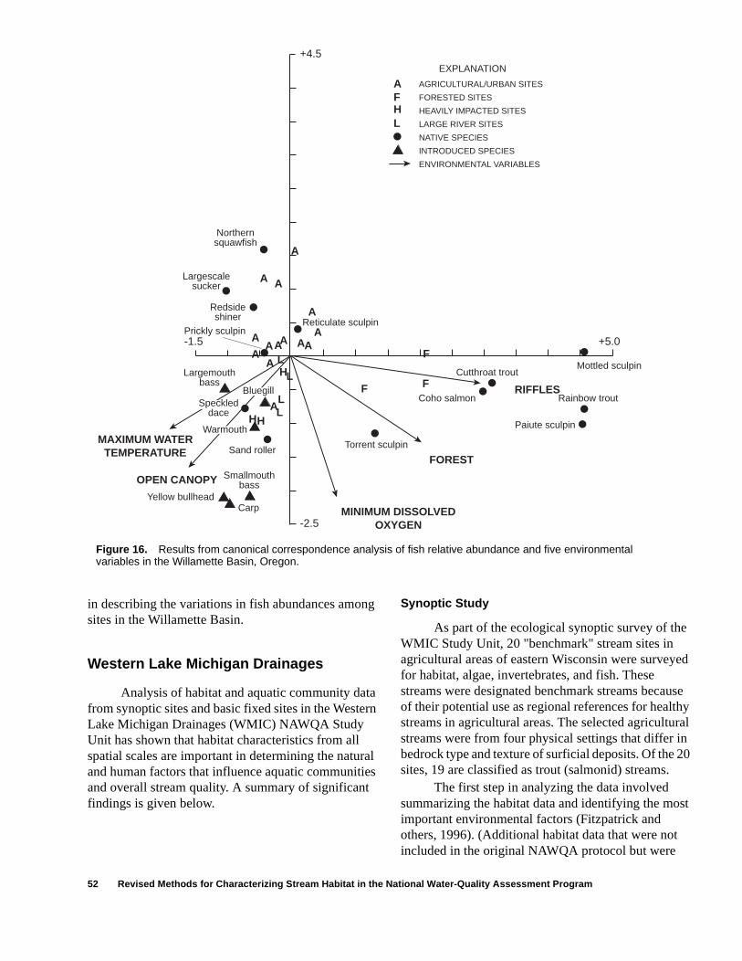
Figure 16. Results from canonical correspondence analysis of fish relative abundance and five environmental variables in the Willamette Basin, Oregon.
L
F
F
F
FOREST
RIFFLES
MINIMUM DISSOLVEDOXYGEN
OPEN CANOPY
MAXIMUM WATERTEMPERATURE
+5.0
-2.5
+4.5EXPLANATION
AGRICULTURAL/URBAN SITES
FORESTED SITES
HEAVILY IMPACTED SITES
LARGE RIVER SITES
NATIVE SPECIES
INTRODUCED SPECIES
ENVIRONMENTAL VARIABLES
A A
A
AAAAA AA
A
AA
L
L
LH
HH
-1.5
Northernsquawfish
Largescalesucker
Redsideshiner Reticulate sculpin
Prickly sculpin
A
AFHL
Largemouthbass
Speckleddace
Warmouth
Sand roller Torrent sculpin
Paiute sculpin
Coho salmon
Cutthroat troutMottled sculpin
Rainbow trout
CarpYellow bullhead
Smallmouthbass
Bluegill
in describing the variations in fish abundances among sites in the Willamette Basin.
Western Lake Michigan Drainages
Analysis of habitat and aquatic community data from synoptic sites and basic fixed sites in the Western Lake Michigan Drainages (WMIC) NAWQA Study Unit has shown that habitat characteristics from all spatial scales are important in determining the natural and human factors that influence aquatic communities and overall stream quality. A summary of significant findings is given below.
Synoptic Study
As part of the ecological synoptic survey of the WMIC Study Unit, 20 "benchmark" stream sites in agricultural areas of eastern Wisconsin were surveyed for habitat, algae, invertebrates, and fish. These streams were designated benchmark streams because of their potential use as regional references for healthy streams in agricultural areas. The selected agricultural streams were from four physical settings that differ in bedrock type and texture of surficial deposits. Of the 20 sites, 19 are classified as trout (salmonid) streams.
The first step in analyzing the data involved summarizing the habitat data and identifying the most important environmental factors (Fitzpatrick and others, 1996). (Additional habitat data that were not included in the original NAWQA protocol but were
52 Revised Methods for Characterizing Stream Habitat in the National Water-Quality Assessment Program

l
e
of
ld
d-
r
11
of
om ced
,
l th
d .
found to be useful included data from STATSGO [texture, erodibility factor, soil drainage, and permeability] and width of the wooded riparian zone at the segment and reach scale.) Next, the data were checked for normality. Various distributions were found—some normal, some log-normal, some neither. Thus, nonparametric statistical methods were employed. Spearman correlation analysis was used to identify habitat characteristics that followed similar distributions among sites. Habitat characteristics that were significantly correlated (Spearman’s rho > 0.50 and p-values < 0.1) were plotted against each other by site identification number to identify site groupings. Next, PCA was done on a subset of characteristics (both raw and ranked data) to explain the overall variance seen in the combination of habitat characteristics. For exploratory purposes, the PCA was done on four subsets of habitat data: (1) 17 habitat characteristics from all scales and three nutrient constituents, (2) 16 basin and segment characteristics, (3) 13 reach characteristics, and (4) 8 water-quality constituents. Axis scores were plotted by physical setting to identify potential groupings of sites. A Kruskal-Wallis test, a nonparametric analysis of variance on rank-transformed data (Iman and Conover, 1983), and the Tukey studentized range test on ranks (Neter and others, 1985) were used to identify significant differences in habitat characteristics between the four physical settings. Finally, using the habitat data, streams were ranked according to Michigan’s qualitative habitat classification system (Michigan Department of Natural Resources, 1991), which is designed to evaluate the effects of nonpoint sources of pollution.
Results from the PCA on all scales of habitat data indicate that the most important habitat characteristics for the benchmark sites are at the basin scale and include land use, soil characteristics, bedrock type, drainage area, and basin storage. Streams that have undergone habitat restoration for fish formed a distinct group on PCA ordination plots of the reach-scale components, indicating that the variability of possible habitat types is reduced when streams are modified by humans to meet the needs of specific aquatic species.
Michigan habitat classification scores (indicators of overall stream condition) indicated that 16 of the 20 sites were suitable reference streams for habitat. No significant differences in scores were found between streams that have undergone habitat
restoration and those that have not. All four physicasettings had the same range of scores.
Indirect gradient analysis was used to comparfish species and habitat data at the benchmark sites(Sullivan and Peterson, 1997). First, fish communitydata were ordinated using DCA. The DCA showed three site groupings, each one associated with one three trout species. The DCA axis 1 and 2 scores correlated with average velocity and percentage of pool, as well as basin-scale characteristics of percentage of sandy surficial deposits, wetland, agriculture, and bedrock type.
In contrast, several community measures for invertebrate data at the benchmark streams such asHilsenhoff’s Biotic Index, did not correlate to bedrockgeology, texture of surficial deposits, or amount of agricultural land use (Rheaume and others, 1996). APCA analysis indicated that 18 of the 20 streams coube divided into three groups relative to stream size, available habitat, and water chemistry: (1) large, warmer streams with slight pollution, (2) deep, mixetemperature streams with minimal pollution, and (3) small, cold, pristine, headwater streams. Two streams were identified as poor representations of benchmark conditions (overlapped with two of the foufrom habitat data analyses alone).
Basic Fixed Sites
Habitat characteristics also were measured at WMIC basic fixed sites during 1993–95. Multiple-reach comparison surveys were done at 3 of the 11sites. Each of the 11 sites had a unique combinationgeology and land use; thus, habitat characteristics frthese sites represented a range of conditions influenby both natural and human factors (Fitzpatrick and Giddings, 1997). Results from Spearman correlationanalysis indicate that, for basin-scale characteristicssignificant correlations were found among land use,soil permeability and erodibility, drainage density, basin shape, stream gradient, flood characteristics, annual mean flow, and base flow. In addition, severabasin-scale characteristics, such as land use, basinstorage, and soil texture and erodibility, correlated withe NAWQA bank stability index. Soil erodibility correlated with dominant substrate type and embeddedness. Habitat evaluation scores correlatewith riparian zone width and the bank stability indexThese correlations indicate the importance of understanding how landscape-scale features in the
Western Lake Michigan Drainages 53

in
or te
tic g
es
of l gy
n,
:
E.,
drainage basin ultimately affect local habitat conditions along a reach.
The availability of temporal and multiple-reach data prompted analyses of significant differences among years and reaches at three sites. In general, most of the significant temporal variability observed was attributed to variable streamflow conditions or problems in identifying bankfull stage. The WMIC sampling strategy required habitat sampling to be done during the spring with invertebrate and algal sampling, after snowmelt runoff but before summer storms. Optimally, this was during low-flow or base-flow conditions, but in some cases base flow was greater during sampling than during the summer months because of prolonged effects from snowmelt on base flow. Even though field conditions appeared similar from year to year, slight variations in streamflow were apparent in measurements that depend on water level, such as depth and velocity.
Comparison of data from the multiple-reach sites indicated whether or not the reach was representative of the segment characteristics. Statistically significant within-segment variability (at the 95-percent confidence level) was found for velocity, embeddedness, bank angle, bank height, and bank vegetative stability. Causes for these differences were thought to be that (1) the reaches were not representative of the segment for these characteristics, or (2) too few measurements were made. These results suggest that there is the potential for variability among multiple reaches for algae, invertebrate, and fish community data as well.
SUMMARY
The NAWQA Program is designed to assess the status of and trends in the Nation’s water quality and to develop an understanding of the major factors that affect observed water-quality conditions and trends. Stream habitat is characterized as part of an integrated physical, chemical, and biological assessment of the Nation’s water quality. The goal of the stream habitat characterization is to provide information on the physical characteristics that, together with chemical and biological characteristics, describe water-quality conditions. Spatial and temporal patterns in habitat characteristics are examined at local, regional, and national scales. The NAWQA stream habitat characterization is based on a spatially hierarchical framework that incorporates habitat data at basin,
segment, reach, and microhabitat scales. This framework provides a basis for national consistencycollection techniques while allowing flexibility in habitat assessment within individual Study Units.
The spatially hierarchical framework of NAWQA habitat characterization requires several methods for data collection. Basin and segment characterization are done by using a GIS data basedata that are derived manually from USGS 7.5-minutopographic maps. Reach and microhabitat data arecollected from measurements made in the field. A subset of reach characteristics is collected at synopsites, with some flexibility to address local questionsand sample a large number of sites while maintaininconsistent methods so that data from basic fixed sitand synoptic sites can be compared. Lastly, these revised methods reflect the experiences of a subsetNAWQA Study Units. Data-collection techniques wilcontinue to evolve as experience grows and technoloadvances.
REFERENCES CITED
Anderson, J.R., Hardy, E.E., Roach, J.T., and Witmer, R.E., 1976, A land use and land cover classification system for use with remote sensor data: U.S. Geological Survey Professional Paper 964, 28 p.
Bailey, R.G., 1983, Delineation of ecosystem regions: Environmental Management, v. 7, p. 365–373.
Baker, N.T., and Frey, J.W., 1997, Fish community and habitat data at selected sites in the White River BasiIndiana, 1993–95: U.S. Geological Survey Open-FileReport 96–653A, 44 p.
Ball, Joseph, 1982, Stream classification guidelines for Wisconsin: Wisconsin Department of Natural Resources Technical Bulletin, 14 p.
Beschta, R.L., and Platts, W.S., 1986, Morphological features of small streams—Significance and functionWater Resources Bulletin, v. 22, p. 369–379.
Biggs, B.J.F., Duncan, M.J., Jowett, I.G., Quinn, J.M., Hickey, C.W., Davies-Colley, R.J., and Close, M.E., 1990, Ecological characterization, classification, andmodeling of New Zealand rivers—An introduction andsynthesis: New Zealand Journal of Marine and Freshwater Research, v. 24, p. 277–304.
Bisson, P.A., Nielsen, J.L., Palmason, R.A., and Grove, L.1982, A system of naming habitat types in small streams, with examples of habitat utilization by salmonids during low streamflow, in Armantrout, N.B., ed., Acquisition and utilization of aquatic habitat inventory information: Western Division, American Fisheries Society, p. 62–73.
54 Revised Methods for Characterizing Stream Habitat in the National Water-Quality Assessment Program
,
,
h, ,
e
ty
se
m rk,
e
l
Bovee, K.D., 1982, A guide to stream habitat analysis using the Instream Flow Incremental Methodology: Fort Collins, Colo., U.S. Fish and Wildlife Service Instream Flow Information Paper 12, FWS/OBS–82/26, 258 p.
Brinker, R.C., and Wolf, P.R., 1977, Elementary surveying (6th ed.): New York, IEP–A Dun-Donnelley Publishers, 568 p.
Burns, D.A., Minshall, G.W., Cushing, C.E., Cummings, K.W., Brock, J.T., and Vannote, R.L., 1984, Tributaries as modifiers of the river continuum concept—Analysis by polar ordination and regression models: Archives of Hydrobiology, v. 99, p. 208–220.
Byl, T.D., and Carney, K.A., 1996, Instream investigations in the Beaver Creek watershed in West Tennessee: U.S. Geological Survey Water-Resources Investigations Report 96–4186, 34 p.
Craig, G.S., and Rankl, J.G., 1978, Analysis of runoff from small drainage basins in Wyoming: U.S. Geological Survey Water-Supply Paper 2056, 70 p.
Cuffney, T.F., Gurtz, M.E., and Meador, M.R., 1993, Methods for collecting benthic invertebrate samples as part of the National Water-Quality Assessment Program: U.S. Geological Survey Open-File Report 93–406, 66 p.
Dahl, T.E., and Johnson, C.E., 1991, Status and trends of wetlands in the conterminous United States, mid-1970’s to mid-1980’s: Washington, D.C., U.S. Fish and Wildlife Service, 28 p.
Dose, J.J., and Roper, B.B., 1994, Long-term changes in low-flow channel widths within the South Umpqua watershed, Oregon: Water Resources Bulletin, v. 30, no. 6, p. 993–1000.
Dunne, Thomas, and Leopold, L.B., 1978, Water in environmental planning: San Francisco, W.H. Freeman and Co., 818 p.
Eash, D.A., 1994, A geographic information system procedure to quantify drainage-basin characteristics: Water Resources Bulletin, v. 30, no. 1, p. 1–8.
Edsall, T.A., Behrendt, T.E., Cholwek, Gary, Frey, J.W., Kennedy, G.W., and Smith, S.B., 1997, Use of remote-sensing techniques to survey the physical habitat of large rivers: U.S. Geological Survey Great Lakes Science Center, Contribution 983, 20 p.
Emmett, W.W., 1975, The channels and waters of the upper Salmon River area, Idaho: U.S. Geological Survey Professional Paper 870–A, 116 p.
Farnsworth, R.K., Thompson, E.S., and Peck, E.L., 1982, Evaporation atlas for the contiguous 48 United States: Office of Hydrology, National Weather Service, National Atmospheric and Oceanic Administration Report NWS 33, 26 p., 4 pls.
Fenneman, N.M., 1946, Physical divisions of the United States: U.S. Geological Survey, scale 1:7,000,000.
Fitzpatrick, F.A., and Giddings, E.M.P., 1997, Stream habitat characteristics of fixed sites in the Western Lake
Michigan Drainages, Michigan and Wisconsin, 1993–95: U.S. Geological Survey Water-Resources Investigations Report 95–4211–B, 58 p.
Fitzpatrick, F.A., Peterson, E.M., and Stewart, J.S., 1996Habitat characteristics of benchmark streams in agricultural areas of eastern Wisconsin: U.S. Geological Survey Water-Resources Investigations Report 96–4038–B, 35 p.
Frayer, W.E., Monahan, T.J., Bowden, D.C., and GraybillF.A., 1983, Status and trends of wetlands and deep-water habitats in the conterminous United States, 1950’s to 1970’s: Fort Collins, Colorado State University, 31 p.
Frissell, C.A., Liss, W.J., Warren, C.E., and Hurley, M.D.,1986, A hierarchical framework for stream habitat classification—Viewing streams in a watershed context: Environmental Management, v. 10, p. 199–214.
Gandolfi, C., and Bischetti, G.B., 1997, Influence of the drainage network identification on geomorphologicalproperties and hydrological response: Hydrological Processes, v. 11, p. 353–375.
Gardiner, V., 1975, Drainage basin morphometry: NorwicEngland, British Geomorphological Research GroupTechnical Bulletin 14, 48 p.
Gebert, W.A., Graczyk, D.J., and Krug, W.R., 1987, Averagannual runoff in the United States, 1951–80: U.S. Geological Survey Hydrologic Investigations Atlas HA–710, scale 1:2,000,000.
Gilliom, R.J., Alley, W.M., and Gurtz, M.E., 1995, Design of the National Water-Quality Assessment Program—Occurrence and distribution of water-qualiconditions: U.S. Geological Survey Circular 1112, 33 p.
Godfrey, A.E., 1977, A physiographic approach to land uplanning: Environmental Geology, v. 2, p. 43–50.
Goldstein, R.M., Stauffer, J.C., Larson, P.R., and Lorenz,D.L., 1996, Relation of physical and chemical characteristics of streams to fish communities in the Red River of the North Basin, Minnesota and North Dakota, 1993–95: U.S. Geological Survey Water-Resources Investigations Report 96–4227, 57 p.
Gordon, N.D., McMahon, T.A., and Finlayson, B.L., 1992, Stream hydrology, An introduction for ecologists: Chichester, U.K., John Wiley & Sons, Ltd., 526 p.
Gorman, O.T., and Karr, J.R., 1978, Habitat structure andstream fish communities: Ecology, v. 59, no. 3, p. 507–515.
Gregory, K.J., and Walling, D.E., 1973, Drainage basin forand process, a geomorphological approach: New YoJohn Wiley & Sons, Inc., 456 p.
Gurtz, M.E., 1994, Design of biological components of thNational Water-Quality Assessment (NAWQA) Program, in Loeb, S.L., and Spacie, A., eds., Biologica
References Cited 55

er .
f
,
al
to
n r
4,
de .
se e 3.
iv.
at , ,
,
.S.
monitoring of aquatic systems, chap. 15: Boca Raton, Fla., Lewis Publishers, p. 323–354.
Gurtz, M.E., Marzolf, R.G., Killingbeck, K.T., Smith, D.L., and McArthur, J.V., 1988, Hydrologic and riparian influences on the import and storage of coarse particulate organic matter in a prairie stream: Canadian Journal of Fisheries and Aquatic Sciences, v. 45, p. 655–665.
Hack, J.T., 1957, Studies of longitudinal stream profiles in Virginia and Maryland: U.S. Geological Survey Professional Paper 294–B, p. 45–97.
Hadley, R.F., and Schumm, S.A., 1961, Sediment sources and drainage basin characteristics in upper Cheyenne River Basin: U.S. Geological Survey Water-Supply Paper 1531–B, 198 p.
Hamilton, Karen, and Bergersen, E.P., 1984, Methods to estimate aquatic habitat variables: Denver, Colo., U.S. Bureau of Reclamation, Environmental Evaluation Project Report DPTS–35–9.
Harrelson, C.C., Rawlins, C.L., and Potyondy, J.P., 1994, Stream channel reference sites—An illustrated guide to field techniques: U.S. Department of Agriculture, Forest Service, Rocky Mountain Forest and Range Experiment Station, General Technical Report RM–245, 61 p.
Harvey, C.A., and Eash, D.A., 1996, Description, instructions, and verification for Basinsoft, a computer program to quantify drainage-basin characteristics: U.S. Geological Survey Water-Resources Investigations Report 95–4287, 25 p.
Hawkins, C.P., 1985, Substrate associations and longitudinal distributions in species of Ephemerellidae (Ephemeroptera: Insecta) from western Oregon: Freshwater Invertebrate Biology, v. 4, p. 181–188.
Higgins, A.L., 1965, Elementary surveying: London, Longmans, Green, and Co.
Hill, M.O., 1979, DECORANA—A Fortran program for detrended correspondence analysis and reciprocal averaging: Ithaca, N.Y., Cornell University.
Hirsch, R.M., Alley, W.M., and Wilber, W.G., 1988, Concepts for a National Water-Quality Assessment Program: U.S. Geological Survey Circular 1021, 42 p.
Hogan, D.L., and Church, Michael, 1989, Hydraulic geometry in small, coastal streams—Progress toward quantification of salmonid habitat: Canadian Journal of Fisheries and Aquatic Sciences, v. 46, no. 5, p. 844–852.
Horton, R.E., 1932, Drainage basin characteristics: Transactions of the American Geophysical Union, v. 13, p. 350–361.
———1945, Erosional development of streams and their drainage basins—Hydrophysical approach to quantita-tive morphology: Bulletin of the Geological Society of America, v. 56, p. 275–370.
Hughes, R.M., and Larsen, D.P., 1988, Ecoregions—An approach to surface water protection: Journal of WatPollution Control Federation, v. 60, no. 4, p. 486–493
Hupp, C.R., 1986, Upstream variation in bottomland vegetation patterns, northwestern Virginia: Bulletin othe Torrey Botanical Club, v. 113, p. 421–430.
Hupp, C.R., and Osterkamp, W.R., 1985, Bottomland vegetation distribution along Passage Creek, Virginiain relation to fluvial landforms: Ecology, v. 66, p. 670–681.
———1996, Riparian vegetation and fluvial geomorphic processes: Geomorphology, v. 14, p. 277–295.
Hutchinson, N.E., 1975, WATSTORE user’s guide, NationWater Data Storage and Retrieval System: U.S. Geological Survey, v. 1, p. B–1—C–9.
Hynes, H.B.N., 1975, The stream and its valley: Verhandlungen Internationale Vereinigung für Theoretische und Angewandte Limnologie, v. 19, p. 1–15.
Iman, R.L., and Conover, W.J., 1983, A modern approachstatistics: New York, John Wiley & Sons, Inc., 497 p.
James, L.A., 1997, Channel incision on the lower AmericaRiver, California, from streamflow gage records: WateResources Research, v. 33, no. 3, p.485–490.
Jennings, M.E., Thomas, W.O., Jr., and Riggs, H.C., 199Nationwide summary of U.S. Geological Survey regional regression equations for estimating magnituand frequency of floods for ungaged sites, 1993: U.SGeological Survey Water-Resources Investigations Report 94–4002, 196 p.
Johnson, R.A., and Wichern, D.W., 1992, Applied multivariate statistical analysis (3d ed.): Englewood Cliffs, N.J., Prentice-Hall, p. 356–395.
Johnson, W.C., Dixon, M.D., Simons, Robert, Jenson, Susan, and Larson, Kevin, 1995, Mapping the responof riparian vegetation to possible flow reductions in thSnake River, Idaho: Geomorphology, v. 13, p. 159–17
Jongman, R.H.G., ter Braak, C.J.F., and van Tongeren, O.F.R., 1995, Data analysis in community and landscape ecology: Cambridge, U.K., Cambridge UnPress, 299 p.
Kaufmann, P.R., and Robison, E.G., 1994, Physical habitassessment, in Klemm, D.J., and Lazorchak, J.M., eds.Environmental monitoring and assessment program1994 pilot field operations manual for streams: U.S. Environmental Protection Agency EPA/620/R–94/004p. 6–1—6–38.
King, P.B., and Beikman, H.M., 1974, Explanatory text toaccompany the geologic map of the United States: UGeological Survey Professional Paper 901, 40 p.
Klingeman, P.C., and MacArthur, R.C., 1990, Sediment transport and aquatic habitat in gravel-bed rivers, in Chang, H.H., and Hill, J.C., eds., Hydraulic engineering: New York, American Society of Civil Engineers, p. 1116–1121.
56 Revised Methods for Characterizing Stream Habitat in the National Water-Quality Assessment Program

, es
., art
r
0 p.
s
d
,
:
ty,
., P., ., s of :
Knox, J.C., 1985, Responses of floods to Holocene climatic change in the upper Mississippi valley: Quaternary Research, v. 23, p. 287–300.
Küchler, A.W., 1970, Potential natural vegetation, in The national atlas of the United States of America: U.S. Geological Survey, p. 89–91.
Langbein, W.B., and Iseri, K.T., 1960, General introduction and hydrologic definitions—Manual of hydrology—Part 1. General surface-water techniques: U.S. Geological Survey Water-Supply Paper 1541–A, 29 p.
Lanka, R.P., Hubert, W.A., and Wesche, T.A., 1987, Relations of geomorphology to stream habitat and trout standing stock in small Rocky Mountain streams: Transactions of the American Fisheries Society, v. 116, no. 1, p. 21–28.
Large, A.R.G., and Petts, G.E., 1994, Rehabilitation of river margins, in Lalow, Peter, and Petts, G.E., eds., The rivers handbook—Hydrological and ecological principles, v. 2: Boston, Mass., Blackwell Scientific Pub., p. 401–418.
Leahy, P.P., Rosenshein, J.S., and Knopman, D.S., 1990, Implementation plan for the National Water-Quality Assessment Program: U.S. Geological Survey Open-File Report 90–174, 10 p.
Leopold, L.B., 1994, A view of the river: Cambridge, Mass., Harvard University Press, 298 p.
Leopold, L.B., and Miller, J.P., 1956, Ephemeral streams—Hydraulic factors and their relation to the drainage net: U.S. Geological Survey Professional Paper 282–A, 37 p.
Leopold, L.B., Wolman, M.G., and Miller, J.P., 1964, Fluvial processes in geomorphology: San Francisco, W.H. Freeman, 522 p.
Lotspeich, F.B., and Platts, W.S., 1982, An integrated land-aquatic classification system: North American Journal of Fisheries Management, v. 2, p. 138–149.
Lowrance, Richard, Todd R.L., Fail, Joseph, Jr., Hendrickson, Ole, Jr., Leonard, R.A., and Asmussen, L.E., 1984, Riparian forests as nutrient filters in agricultural watersheds: BioScience, v. 34, no. 6, p. 374–377.
Maret, T.R., 1997, Characteristics of fish assemblages and related environmental variables for streams of the Upper Snake River Basin, Idaho and Western Wyoming, 1993–95: U.S. Geological Survey Water-Resources Investigations Report 97–4087, 50 p.
Maret, T.R., Robinson, C.T., Minshall, G.W., 1997, Fish assemblages and environmental correlations in least-disturbed streams of the Upper Snake River Basin: Transactions of the American Fisheries Society v. 126, no. 2, p. 200–216.
McCain, M., Fuller, D., Decker, L., and Overton, K., 1990Stream habitat classification and inventory procedurfor northern California: U.S. Department of Agriculture, R–5’s Fish Habitat Relationships Technical Bulletin 1, 15 p.
Meador, M.R., Cuffney, T.F., and Gurtz, M.E., 1993, Methods for sampling fish communities as part of theNational Water-Quality Assessment Program: U.S. Geological Survey Open-File Report 93–104, 40 p.
Meador, M.R., Hupp, C.R., Cuffney, T.F., and Gurtz, M.E1993, Methods for characterizing stream habitat as pof the National Water-Quality Assessment Program: U.S. Geological Survey Open-File Report 93–408, 48 p.
Michigan Department of Natural Resources, 1991, Qualitative biological and habitat survey protocols fowadable streams and rivers: Great Lakes and Environmental Assessment Section Procedure 51, 4
Montgomery, D.R., and Buffington, J.M., 1993, Channel classification, prediction of channel response, and assessment of channel condition: Timber, Fish, and Wildlife TFW–SH10–93–002 [variously paged].
Mueller-Dombois, Dieter, and Ellenberg, Heinz, 1974, Aimand methods of vegetation ecology: New York, JohnWiley & Sons, Inc., 547 p.
Neter, J., Wasserman, W., and Kutner, M.H., 1985, Applielinear statistical models—Regression, analysis of variance, and experimental designs (2d ed.): Homewood, Ill., R.D. Irwin Publishers, 1,127 p.
Novak, C.E., 1985, WRD data reports preparation guide:U.S. Geological Survey Water Resources Division, p. 43–46.
Ohio Environmental Protection Agency, 1989, Biological criteria for the protection of aquatic life, v. III, Standardized biological field sampling and laboratorymethods for assessing fish and invertebrate communities: Ohio Environmental Protection Agency58 p.
Olson-Rutz, K.M., and Marlow, C.B., 1992, Analysis and interpretation of stream channel cross-sectional dataNorth American Journal of Fisheries Management, v. 12, no. 1, p. 55–61.
Omernik, J.M., 1987, Ecoregions of the conterminous United States: Annals of the Association of AmericanGeographers, v. 77, p. 118–125.
Orth, D.J., 1983, Aquatic habitat measurements, in Nielsen, L.A., and Johnson, D.L., eds., Fisheries techniques, Chapter 4: Bethesda, Md., American Fisheries Sociep. 61–84.
Osborne, L.L., Dickson, B., Ebbers, M., Ford, R., Lyons, JKline, D., Rankin, E., Ross, D., Sauer, R., Seelbach, Speas, C., Stefanavage, T., Waite, J., and Walker, S1991, Stream habitat assessment programs in statethe American Fisheries Society North Central DivisionFisheries, v. 16, p. 28–35.
References Cited 57

, .
98.
y
al t
ct rth
of
s
es n s
n in of .
Osborne, L.L., and Wiley, M.J., 1992, Influence of tributary spatial position on the structure of warmwater fish communities: Canadian Journal of Fisheries and Aquatic Sciences, v. 49, p. 671–681.
Plafkin, J.L., Barbour, M.T., Porter, K.D., Gross, S.K., and Hughes, R.M., 1989, Rapid bioassessment protocols for use in streams and rivers—Benthic macroinvertebrates and fish: U.S. Environmental Protection Agency EPA/444/4–89–001 [variously paged].
Platts, W.S., Armour, Carl, Booth, G.D., Bryant, Mason, Bufford, J.L., Cuplin, Paul, Jensen, Sherman, Lienkaemper, G.W., Minshall, G.W., Monsen, S.B., Nelson, R.L., Sedell, J.R., and Tuhy, J.S., 1987, Methods for evaluating riparian habitats with applications to management: Ogden, Utah, U.S. Forest Service, General Technical Report INT–221, 177 p.
Platts, W.S., Megahan, W.F., and Minshall, G.W., 1983, Methods for evaluating stream, riparian, and biotic conditions: Ogden, Utah, U.S. Forest Service, General Technical Report INT–138, 70 p.
Porter, S.G., Cuffney, T.F., Gurtz, M.E., and Meador, M.R., 1993, Methods for collecting algal samples as part of the National Water-Quality Assessment Program: U.S. Geological Survey Open-File Report 93–409, 39 p.
Quinn, J.M., and Hickey, C.W., 1990, Characterization and classification of benthic invertebrate communities in 88 New Zealand rivers in relation to environmental factors: New Zealand Journal of Marine and Freshwater Research, v. 24, p. 387–409.
Rantz and others, 1982, Measurement and computation of streamflow—v. 1 Measurement of stage and discharge: U.S. Geological Survey Water-Supply Paper 2175, p. 273–284.
Rheaume, S.J., Lenz, B.N., and Scudder, B.C., 1996, Benthic invertebrates of benchmark streams in agricultural areas of eastern Wisconsin—Western Lake Michigan Drainages: U.S. Geological Survey Water-Resources Investigations Report 96–4038–C, 39 p.
Ritter, D.F., 1978, Process geomorphology: Dubuque, Iowa, Wm. C. Brown, 603 p.
Roper, B.B., and Scarnecchia, D.L., 1995, Observer variability in classifying habitat types in stream surveys: North American Journal of Fisheries Management, v. 15, no. 1, p. 49–53.
Rosgen, D.L., 1994, A classification of natural rivers: Catena, v. 22, p. 169–199.
———1997, Applied river morphology: Pagosa Springs, Colo., Wildland Hydrology [variously paged].
Schumm, S.A., 1956, Evolution of drainage systems and slopes in badlands at Perth Amboy, New Jersey: Geological Society of America Bulletin, v. 67, p. 597–646.
———1960, The shape of alluvial channels in relation to sediment type: U.S. Geological Survey Professional Paper 352–B, 30 p.
———1963, Sinuosity of alluvial channels on the Great Plains: Geological Society of America Bulletin, v. 74,p. 1089–1100.
Schumm, S.A., and Lichty, R.W., 1965, Time, space, andcausality in geomorphology: American Journal of Science, v. 263, p. 110–119.
Seaber, P.R., Kapino, F.P., and Knapp, G.L., 1984, Statehydrologic unit maps: U.S. Geological Survey Open-File Report 84–708, 198 p.
Seibert, T.F., Sidle, J.G., and Savidge, J.A., 1996, Inexpensive aerial videography acquisition, analysisand reproduction: Wetlands, v. 16, no. 2, p. 245–250
Sheldon, A.L., 1968, Species diversity and longitudinal succession in stream fishes: Ecology, v. 49, p. 193–1
Shreve, R.L., 1967, Infinite topologically random channelnetworks: Journal of Geology, v. 75, p. 178–186.
Simon, Andrew, and Hupp, C.R., 1992, Geomorphic and vegetative recovery processes along modified streamchannels of west Tennessee: U.S. Geological SurveOpen-File Report 91–502, 142 p.
Simonson, T.D., Lyons, John, and Kanehl, P.D., 1994a, Guidelines for evaluating fish habitat in Wisconsin streams: U.S. Department of Agriculture, North CentrForest Experiment Station, General Technical ReporNC–164, 36 p.
———1994b, Quantifying fish habitat in streams—Transespacing, sample size, and a proposed framework: NoAmerican Journal of Fisheries Management, v. 14, no. 3, p. 607–615.
Skinner, E.L., and Borman, R.G., 1973, Water resources Wisconsin—Lake Michigan Basin: U.S. Geological Survey Hydrologic Investigations Atlas HA–432, 4 sheets.
Smith, K.G., 1950, Standards for grading texture of erosional topography: American Journal of Science, v. 248, p. 655–668.
Stauffer, J.C., and Goldstein, R.M., 1997, Comparison ofthree qualitative habitat indices and their applicabilityto prairie streams: North American Journal of FisherieManagement, v. 17, no. 2, p. 348–361.
Strahler, A.N., 1957, Quantitative analysis of watershed geomorphology: Transactions of the American Geophysical Union, v. 38, p. 913–920.
Strichler, G.S., 1959, Use of the densiometer to estimatedensity of forest canopy on permanent sample plots:U.S. Department of Agriculture, Forest Service, Research Note INT–180, 5 p.
Sullivan, D.J., and Peterson, E.M., 1997, Fish communitiof benchmark streams in agricultural areas of easterWisconsin: U.S. Geological Survey Water-ResourceInvestigations Report 96–4038–D, 23 p.
Sweeney, B.W., 1993, Effects of streamside vegetation omacroinvertebrate communities of White Clay Creek eastern North America: Proceedings of the AcademyNatural Sciences of Philadelphia, v. 144, p. 291–340
58 Revised Methods for Characterizing Stream Habitat in the National Water-Quality Assessment Program
,
al
Tate, C.M., and Heiny, J.S., 1995, The ordination of benthic invertebrate communities in the South Platte River Basin in relation to environmental factors: Freshwater Biology, v. 33, p. 439–454.
Teti, Patrick, 1984, Time-variant differences in chemistry among four smaller streams: Water Resources Research, v. 20, p. 347–359.
Tonn, W.M., 1990, Climate change and fish communities—A conceptual framework: Transactions of the American Fisheries Society, v. 119, p. 337–352.
Trimble, S.W., 1997, Stream channel erosion and change resulting from riparian forests: Geology, v. 25, no. 5, p. 467–469.
Uren, J., and Price, W.F., 1984, Calculations for engineering surveys: New York, Van Nostrand Reinhold, 309 p.
U.S. Department of Agriculture, 1972, Land resource regions and major land resource areas of the United States: U.S. Department of Agriculture Handbook 296, 156 p.
———1991, State soil geographic data base (STATSGO), data user’s guide: U.S. Department of Agriculture, Soil Conservation Service Miscellaneous Publication 1492, 88 p., scale 1:250,000.
———1995, A guide to field identification of bankfull stage in the western United States: Rocky Mountain Forest and Range Experiment Station Stream Systems Tech-nology Center, Forest Service videotape, approx. 30 minutes.
Wendland, W.M., Kunkel, K.E., Conner, G., Decker, W.L.,Hillaker, H., Nabor-Knox, P., Nurnberger, F.V., RogersJ., Scheeringa, K., and Zandlo, J., 1992, Mean 1961–1990 temperature and precipitation over the upper Midwest: Midwest Climate Center Research Report 92–01, 27 p.
Williams, G.P., 1978, Bank-full discharge of rivers: Water Resources Research, v. 14, no. 6, p. 1141–1154.
Wolman, M.G., 1954, A method for sampling coarse river-bed material: Transactions of the American Geophysical Union, v. 35, p. 951–956.
Wolman, M.G., and Gerson, R., 1978, Relative scales of time and effectiveness of climate in watershed geomorphology: Earth Surface Processes, v. 3, p. 189–208.
Wolman, M.G., and Leopold, L.B., 1957, River flood plains—Some observations on their formation: U.S. Geological Survey Professional Paper 282–C, p. 87–109.
Wolman, M.G., and Miller, J.P., 1960, Magnitude and frequency of forces in geomorphic processes: Journof Geology, v. 68, p. 54–57.
Ying, T.C., 1971, Formation of riffles and pools: Water Resources Research, v. 7, p. 1567–1574.
References Cited 59

FIELD FORMS
60 Revised Methods for Characterizing Stream Habitat in the National Water-Quality Assessment Program

Field Forms 61
USGS Field Form 1. Basin Characterization Page 1 of 2[Fill out one form for each site. Items in bold are required for NAWQA national data aggregation. Circle units of measure where appropriate. Abbreviations in parentheses refer to parameter codes in NWIS or the NAWQA data dictionary file]
1. Study Unit (SUID): __ __ __ __ 2. Site type (SITYPE): BFS IFS SYN
3. Station ID (C001 or STAID): ___________ 4. HUC code (C020): ___________________ 5. Station name (C900):_________________________________________________________
6. Reference location: longitude (C010): ___________ latitude (C009): __________ elevation (meters above NGVD) (C016): _____________
7. State FIPS code (C007):__________ 8. County FIPS code (C008): _________ 9. State (STATE): _________ 10. County (COUNTY):_____________________11. Township (TWN): _________ 12. Range (RANGE): ___________ 13. Section (SEC): ___________
14. Quad topographic sheets covering basin (QUAD): Quad name Scale Year
________________________________________________________ ________ ________________________________________________________________ ________ ________________________________________________________________ ________ ________________________________________________________________ ________ ________________________________________________________________ ________ ________________________________________________________________ ________ ________________________________________________________________ ________ ________
15. File name(s) and path where these data can be found: ________________________________________________________________________
16. Contact person for site and basin data: _____________________________________
17. Total drainage area (C808): _______________ square kilometers square milesContributing drainage area (C809): _______________
18. Drainage area method (DRAREAMD): map year Computation method list (circle one): manual vector rasterSource-map-scale list (circle one): 1:24k 1:48k 1:100k 1:250k
19. Average annual runoff (RUNOFF): _________________ centimeters inches20. Average annual runoff method (RUNOFFMD): GAGE WTGAGE REFERENCE OTHER __________21. Length of record for average annual runoff: Beginning year (BYRUNOFF) __________
Ending year (EYRUNOFF) __________22. Average annual air temperature (TEMP): _________________ °C
23. Average annual air temperature method (TEMPMD): THIESSEN NEIGHBOR ISOHYET REFERENCE
AVG KRIG OTHER ____________24. Length of record for average annual air temperature:
Beginning year (BYTEMP) __________Ending year (EYTEMP) __________
25. Average annual precipitation (PRECIP): _______________ centimeters26. Average annual precipitation method (PRECIPMD): THIESSEN NEIGHBOR ISOHYET REFERENCE
AVG KRIG OTHER ____________27. Length of record for average annual precipitation:
Beginning year (BYPRECIP) __________Ending year (EYPRECIP) __________

62 Revised Methods for Characterizing Stream Habitat in the National Water-Quality Assessment Program
USGS Field Form 1. Basin Characterization—Continued Page 2 of 2
28. Average annual Class A pan evaporation (EVAPAN): _____________ centimeters inches29. Average annual evaporation method (EVAPANMD): THIESSEN NEIGHBOR ISOHYET REFERENCE
AVG KRIG OTHER ____________30. Length of record for average annual Class A pan evaporation:
Beginning year (BYEVAPAN): __________ Ending year (EYEVAPAN): _____________
31. Basin length (BLENG): ________________ kilometers miles32. Basin length method (BLENGMD): map year _______
Computation-method list (circle one): manual vector rasterSource-map-scale list (circle one): 1:24k 1:48k 1:100k 1:250k
33. Minimum elevation in the basin (MNELEV):__________ meters above NGVD (above datum > 0.0; below datum < 0.0)34. Minimum elevation method (MNELEVMD): map year ________
Computation-method list (circle one): manual vector rasterSource-map-scale list (circle one): 1:24k 1:48k 1:100k 1:250k
35. Maximum elevation in the basin (MXELEV): __________meters above NGVD (above datum > 0.0; below datum < 0.0)36. Maximum elevation method (MXELEVMD): map year _________
Computation-method list (circle one): manual vector rasterSource-map-scale list (circle one): 1:24k 1:48k 1:100k 1:250k
37. Basin relief ratio (RELRAT): ____________________38. Drainage shape (DRNSHAPE): ____________________39. Stream length (SLENG): ______________________ kilometers (> 0.0)40. Stream length method (SLENGMD): map year __________
Computation-method list (circle one): manual vector rasterSource-map-scale list (circle one): 1:24k 1:48k 1:100k 1:250k
41. Cumulative perennial stream length (PSLENG): _________________ kilometers (> 0.0)42. Cumulative perennial stream length method (PSLENGMD): map year _________
Computation-method list (circle one): manual vector rasterSource-map-scale list (circle one): 1:24k 1:48k 1:100k 1:250k
43. Drainage density (DRNDENS): ___________________ kilometers-1
44. Drainage texture (DRNTEX): ____________ contours/kilometer (> 0.00)45. Entire stream gradient (SLOPE): _________ meters/kilometer46. Estimated flow characteristics: Beginning period of record (QBDATE): _______ Ending period of record (QEDATE): _______
47. Method(s) for estimating streamflow characteristics, such as from gaging-station data or list references if State or regional equations were used (FLOWMD):
_______________________________________________________________________________
Recurrence interval (in years)
Peak flow(m3/s ft3/s)
Flood volume(m3 ft3)
7-day low flow(m3/s ft3/s)
1 ________ (QP1) 2 ________ (QP2) ________ (QV2) ________ (Q7L2)5 ________ (QP5) ________ (QV5) ________ (Q7L5)
10 ________ (QP10) ________ (QV10) ________ (Q7L10)25 ________ (QP25) ________ (QV25) ________ (Q7L25)50 ________ (QP50) ________ (QV50) ________ (Q7L50)
100 ________ (QP100) ________ (QV100) ________ (Q7L100)

Field Forms 63
USGS Field Form 2. Segment Characterization Page 1 of 2[Fill out one form for each site. Items in bold are required for NAWQA national data aggregation. Circle units of measure where appropriate. Abbreviations in parentheses refer to parameter codes in the NAWQA data dictionary]
1. Study Unit (SUID): __ __ __ __ 2. Station ID (C001 or STAID): __________________
3. Station name (C900): __________________________________________________________ 4. EPA RF3 segment code (SEGCODE): ____________
5. Location of segment boundaries (degrees, minutes, seconds): Upstream end: latitude (USLAT) __________ longitude (USLONG) ___________Downstream end: latitude (DSLAT) __________ longitude (DSLONG) ___________
6. Segment boundary location method (LOCMD): map year _______ Computation-method list (circle one): manual field GIS-vector GIS-raster Source-map-scale list (circle one): 1:24k 1:48k 1:100k 1:250k 7. Segment length (SEGLENG): _____________ kilometers meters miles feet 8. Segment length method (SEGLENMD): map year _______
Computation-method list (circle one): manual field GIS-vector GIS-rasterSource-map-scale list (circle one): 1:24k 1:48k 1:100k 1:250k
9. Curvilinear channel length and distance to reference locations (upstream is negative, downstream is positive):
Upstream end (USDIST): ____________ kilometers meters miles feetDownstream end (DSDIST): ____________ kilometers meters miles feetTotal curvilinear channel length (SEGCUR): __________ kilometers meters miles feet
10. Curvilinear channel length method (SEGCURMD): map year _______Computation-method list (circle one): manual field GIS-vector GIS-rasterSource-map-scale list (circle one): 1:24k 1:48k 1:100k 1:250k
11. Upstream and downstream elevation above NGVD:Upstream end (USELEV): _________ meters feet Downstream end (DSELEV): _______ meters feet
12. Elevation method (SELEVMD): map year _______Computation-method list (circle one): manual field GIS-vector GIS-rasterSource-map-scale list (circle one): 1:24k 1:48k 1:100k 1:250k
13. Channel sinuosity (SINUOS): ____________ (dimensionless)14. Segment gradient (GRADIENT): ____________ (dimensionless)15. Water management features (in "Wmf" file):
Identification(WMFID)
Type (WMFTYPE)
Description (WMFDES)
Start date (WMFBDATE)
End date (WMFEDATE)
Distance1 (WMFDIST)(km mi)
1Distance, in kilometers, from reference location—upstream is negative and downstream is positive.
16. Strahler stream order (ORDER): __________17. Strahler stream-order method (ORDERMD): map year _______
Computation-method list (circle one): manual field GIS-vector GIS-rasterSource-map-scale list (circle one): 1:24k 1:48k 1:100k 1:250k
18. Link (Shreve stream order) (LINK): ___________
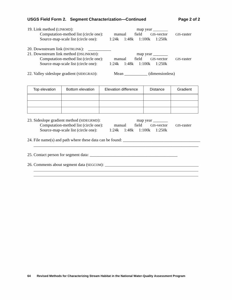
64 Revised Methods for Characterizing Stream Habitat in the National Water-Quality Assessment Program
USGS Field Form 2. Segment Characterization—Continued Page 2 of 2
19. Link method (LINKMD): map year _______Computation-method list (circle one): manual field GIS-vector GIS-rasterSource-map-scale list (circle one): 1:24k 1:48k 1:100k 1:250k
20. Downstream link (DSTRLINK): ___________21. Downstream link method (DSLINKMD): map year _______
Computation-method list (circle one): manual field GIS-vector GIS-rasterSource-map-scale list (circle one): 1:24k 1:48k 1:100k 1:250k
22. Valley sideslope gradient (SIDEGRAD): Mean ___________ (dimensionless)
23. Sideslope gradient method (SIDEGRMD): map year _______Computation-method list (circle one): manual field GIS-vector GIS-rasterSource-map-scale list (circle one): 1:24k 1:48k 1:100k 1:250k
24. File name(s) and path where these data can be found: _____________________________________ _______________________________________________________________________________
25. Contact person for segment data: __________________________________________
26. Comments about segment data (SEGCOM):
Top elevation Bottom elevation Elevation difference Distance Gradient

Field Forms 65
USGS Field Form 3. Reach Characterization Page 1 of 2[Fill out one form for each reach. Items in bold are required for NAWQA national data aggregation. Circle units of measure where appropriate. Abbreviations in parentheses refer to parameter codes in the NAWQA data dictionary]
1. Study Unit (SUID): _________ 2. Station ID (C001 or STAID): _________________ 3. Date (DATE): _____ - _____ - ______ (mm-dd-yyyy) 4. Reach (REACHSEQ): A B C D E 5. Station name (C900): __________________________________________________________ 6. Description of reference location (REFLOC): ____________________________________________ 7. Investigators (INVEST): ___________________________________________________ 8. Quality of habitat sampling effort (RCHQUAL): (circle one) excellent good fair poor 9. Comments on habitat sampling or conditions (REACHCOM): _____________________________
____________________________________________________________________________________________________________________________________________________________
10. Stage (STAGE): ________ meters feet 11. Method (STAGEMD): ADR staff tape-down12. Instantaneous discharge (DISCH): _______ m3/s ft3/s13. Method (DISCHMD): gage wading rod estimated _____________ other ______________14. Channel modification at reach (CHMOD): concrete lined stabilized dredged
channelized, not stabilized wing dams lightly affected not modified15. Mean channel width (MCW): 1 ____ 2 _____ 3 _____ mean ______ meters feet16. Curvilinear reach length (REACHLEN): _______________ meters feet17. Distance between transects (TRANDIS): ________ meters feet18. Curvilinear distance from reference location to reach (upstream is negative, downstream is
positive): Upstream end (USRCHEND) meters feetDownstream end (DSRCHEND) _______ meters feet
19. Location of boundary markers (circle one for each):Upstream boundary (USBMBK) left right bothDownstream boundary (DSBMBK) left right both
20. Boundary marker descriptions (USBMDESC, DSBMDESC): ______________________________________________________________________________________________________________________________________________________________________________________________
21. Water-surface gradient (RCHGRAD): _________ thalweg gradient (THGRAD): ________22. Method for reach gradient (RCHGRAMD): surveying level clinometer hand level other23. Geomorphic channel units (in "Gcu" file), length measured in (circle one): meters feet
Sequence(GCUSEQ)
Type (circle one)(GCUTYPE)
Length(GCULEN)
Sequence(GCUSEQ)
Type (circle one)(GCUTYPE)
Length(GCULEN)
1 pool riffle run 11 pool riffle run
2 pool riffle run 12 pool riffle run
3 pool riffle run 13 pool riffle run
4 pool riffle run 14 pool riffle run
5 pool riffle run 15 pool riffle run
6 pool riffle run 16 pool riffle run
7 pool riffle run 17 pool riffle run
8 pool riffle run 18 pool riffle run
9 pool riffle run 19 pool riffle run
10 pool riffle run 20 pool riffle run

66 Revised Methods for Characterizing Stream Habitat in the National Water-Quality Assessment Program
USGS Field Form 3. Reach Characterization Page 2 of 2
24. Diagrammatic map: Station ID _________________ Reach A B C D E Date ___-___-___
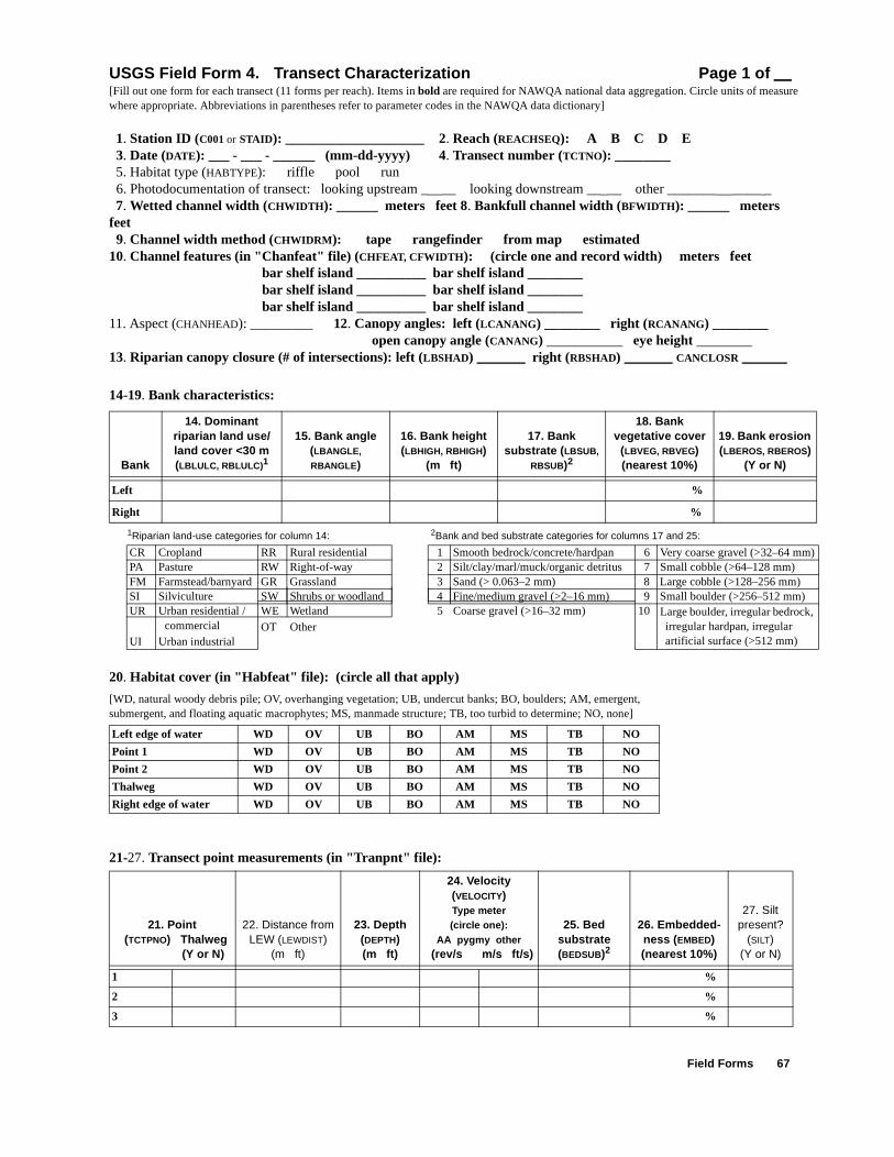
))
mm) mm)k,
USGS Field Form 4. Transect Characterization Page 1 of [Fill out one form for each transect (11 forms per reach). Items in bold are required for NAWQA national data aggregation. Circle units of measure where appropriate. Abbreviations in parentheses refer to parameter codes in the NAWQA data dictionary]
1. Station ID (C001 or STAID): ____________________ 2. Reach (REACHSEQ): A B C D E 3. Date (DATE): ___ - ___ - ______ (mm-dd-yyyy) 4. Transect number (TCTNO): ________ 5. Habitat type (HABTYPE): riffle pool run 6. Photodocumentation of transect: looking upstream _ __ looking downstream __ __ other _______ ____ _ 7. Wetted channel width (CHWIDTH): ______ meters feet 8. Bankfull channel width (BFWIDTH): ______ meters feet 9. Channel width method (CHWIDRM): tape rangefinder from map estimated10. Channel features (in "Chanfeat" file) (CHFEAT, CFWIDTH): (circle one and record width) meters feet bar shelf island __________ bar shelf island ________ bar shelf island __________ bar shelf island ________ bar shelf island __________ bar shelf island ________11. Aspect (CHANHEAD): _________ 12. Canopy angles: left (LCANANG) ________ right (RCANANG) ________ open canopy angle (CANANG) eye height 13. Riparian canopy closure (# of intersections): left (LBSHAD) right (RBSHAD) CANCLOSR
14-19. Bank characteristics:
1Riparian land-use categories for column 14: 2Bank and bed substrate categories for columns 17 and 25:
Bank
14. Dominant riparian land use/land cover <30 m(LBLULC, RBLULC)1
15. Bank angle (LBANGLE,
RBANGLE)
16. Bank height (LBHIGH, RBHIGH)
(m ft)
17. Bank substrate (LBSUB,
RBSUB)2
18. Bank vegetative cover
(LBVEG, RBVEG)(nearest 10%)
19. Bank erosion (LBEROS, RBEROS)
(Y or N)
Left %
Right %
CR Cropland RR Rural residential 1 Smooth bedrock/concrete/hardpan 6 Very coarse gravel (>32–64 mmPA Pasture RW Right-of-way 2 Silt/clay/marl/muck/organic detritus 7 Small cobble (>64–128 mmFM Farmstead/barnyard GR Grassland 3 Sand (> 0.063–2 mm) 8 Large cobble (>128–256SI Silviculture SW Shrubs or woodland 4 Fine/medium gravel (>2–16 mm) 9 Small boulder (>256–512UR
UI
Urban residential /commercial
Urban industrial
WEOT
WetlandOther
5 Coarse gravel (>16–32 mm) 10Large boulder, irregular bedrocirregular hardpan, irregular artificial surface (>512 mm)
20. Habitat cover (in "Habfeat" file): (circle all that apply)
[WD, natural woody debris pile; OV, overhanging vegetation; UB, undercut banks; BO, boulders; AM, emergent, submergent, and floating aquatic macrophytes; MS, manmade structure; TB, too turbid to determine; NO, none]
21-27. Transect point measurements (in "Tranpnt" file):
Left edge of water WD OV UB BO AM MS TB NO
Point 1 WD OV UB BO AM MS TB NO
Point 2 WD OV UB BO AM MS TB NO
Thalweg WD OV UB BO AM MS TB NO
Right edge of water WD OV UB BO AM MS TB NO
21. Point (TCTPNO) Thalweg
(Y or N)
22. Distance from LEW (LEWDIST)
(m ft)
23. Depth(DEPTH)(m ft)
24. Velocity(VELOCITY)Type meter(circle one):
AA pygmy other (rev/s m/s ft/s)
25. Bed substrate(BEDSUB)2
26. Embedded-ness (EMBED)(nearest 10%)
27. Silt present?
(SILT)(Y or N)
1 %
2 %
3 %
Field Forms 67
Fitzpatrick and others—Revised Methods for Characterizing Stream Habitat in the NAWQA Program—USGS/WRIR 98-4052