rf concrete surfaces
TRANSCRIPT
Program RF-CONCRETE Surfaces © 2013 Dlubal Software GmbH
Add-on Module
RF-CONCRETE Surfaces Reinforced Concrete Design
Program Description
Version October 2013
All rights, including those of translations, are reserved.
No portion of this book may be reproduced – mechanically, electronically, or by any other means, including photocopying – without written permission of DLUBAL SOFTWARE GMBH. © Dlubal Software GmbH Am Zellweg 2 D-93464 Tiefenbach Tel.: +49 9673 9203-0 Fax: +49 9673 9203-51 E-mail: [email protected] Web: www.dlubal.com


3
Contents
Contents Page
Contents Page
Program RF-CONCRETE Surfaces © 2013 Dlubal Software GmbH
1. Introduction 6 1.1 Add-on module RF-CONCRETE Surfaces 6 1.2 RF-CONCRETE Surfaces Team 7 1.3 Using the Manual 8 1.4 Opening RF-CONCRETE Surfaces 8 2. Theoretical Background 10 2.1 Type of Model 10 2.2 Design of 1D and 2D Structural
Components 11 2.3 Walls (Diaphragms) 14 2.3.1 Design Internal Forces 14 2.3.2 Two-Directional Reinforcement Meshes
with k > 0 17 2.3.3 Two-Directional Reinforcement Meshes
with k < 0 20 2.3.4 Possible Load Situations 21 2.3.5 Design of the Concrete Compression
Strut 24 2.3.6 Determination of Required
Reinforcement 24 2.3.7 Reinforcement Rules 25 2.4 Plates 28 2.4.1 Design Internal Forces 28 2.4.2 Design of Stiffening Moment 33 2.4.3 Determination of Statically Required
Reinforcement 36 2.4.4 Shear Design 37 2.4.4.1 Design Shear Resistance Without Shear
Reinforcement 38 2.4.4.2 Design Shear Resistance with Shear
Reinforcement 42 2.4.4.3 Design of Concrete Strut 44 2.4.4.4 Example for Shear Design 44 2.4.5 Reinforcement Rules 46 2.5 Shells 48 2.5.1 Design Concept 48 2.5.2 Lever arm of the Internal Forces 49 2.5.3 Determination of Design Membrane
Forces 54 2.5.3.1 Design Moments 57 2.5.3.2 Design Axial Forces 59
2.5.3.3 Lever of Internal Forces 59 2.5.3.4 Membrane Forces 60 2.5.3.5 Design Membrane Forces 61 2.5.4 Analysis of Concrete Struts 62 2.5.5 Required Longitudinal Reinforcement 63 2.5.6 Shear Design 64 2.5.7 Statically Required Longitudinal
Reinforcement 66 2.5.8 Minimum Longitudinal Reinforcement 66 2.5.9 Reinforcement to be Used 67 2.6 Serviceability Limit State 69 2.6.1 Design Internal Forces 69 2.6.2 Principal Internal Forces 71 2.6.3 Provided Reinforcement 72 2.6.4 Serviceability Limit State Designs 72 2.6.4.1 Input Data for Example 72 2.6.4.2 Check of Principal Internal Forces 72 2.6.4.3 Required Reinforcement for ULS 73 2.6.4.4 Specification of a Reinforcement 74 2.6.4.5 Check of the Provided Reinforcement for
SLS 75 2.6.4.6 Selection of the Concrete Strut 76 2.6.4.7 Limitation of Concrete Pressure Stress 77 2.6.4.8 Limitation of the Reinforcing Steel Stress 80 2.6.4.9 Minimum Reinforcement for Crack
Control 81 2.6.4.10 Checking the Rebar Diameter 84 2.6.4.11 Design of Rebar Spacing 86 2.6.4.12 Check of Crack Width 87 2.6.5 Governing Effects of Actions 91 2.7 Deformation analysis with RF-CONCRETE
Deflect 92 2.7.1 Basic Material and Geometric
Assumptions 92 2.7.2 Design Internal Forces 92 2.7.3 Critical Surface 92 2.7.4 Cross-Section Properties 93 2.7.5 Long-Term Effects 93 2.7.5.1 Creep 93

4
Contents
Program RF-CONCRETE Surfaces © 2013 Dlubal Software GmbH
Contents Page
Contents Page
2.7.5.2 Shrinkage 93 2.7.6 Distribution Coefficient 95 2.7.7 Cross-Section Properties for Deformation
Analysis 96 2.7.8 Material Stiffness Matrix D 97 2.7.9 Positive Definite Test 97 2.7.10 Example 98 2.7.10.1 Geometry 98 2.7.10.2 Materials 98 2.7.10.3 Selection of the Design Internal Forces 99 2.7.10.4 Determination of Critical Surface 99 2.7.10.5 Cross-Section Properties (Cracked and
Uncracked State) 100 2.7.10.6 Consideration of Shrinkage 102 2.7.10.7 Calculation of Distribution Coefficient
(Damage Parameter) 103 2.7.10.8 Final Cross-Section Properties 104 2.7.10.9 Stiffness Matrix of the Material 106 2.8 Nonlinear Method 107 2.8.1 General 107 2.8.2 Equations and Methods of
Approximations 107 2.8.2.1 Theoretical Approaches 107 2.8.2.2 Flowchart 109 2.8.2.3 Method for Solving Nonlinear Equations 110 2.8.2.4 Convergence Criteria 111 2.8.3 Material Properties 113 2.8.3.1 Concrete in Compression 113 2.8.3.2 Concrete in Tension 113 2.8.3.3 Tension Stiffening: Stiffening Effect of
Concrete in Tension 115 2.8.3.4 Reinforcing Steel 119 2.8.4 Creep and Shrinkage 120 2.8.4.1 Consideration of Creep 120 2.8.4.2 Consideration of Shrinkage 123 3. Input Data 127 3.1 General Data 127 3.1.1 Ultimate Limit State 130 3.1.2 Serviceability Limit State 131
3.1.2.1 Analytical Method 132 3.1.2.2 Nonlinear Method 134 3.1.3 Details 137 3.2 Materials 138 3.3 Surfaces 141 3.3.1 Analytical Method 141 3.3.2 Nonlinear Method 144 3.4 Reinforcement 148 3.4.1 Reinforcement Ratios 149 3.4.2 Reinforcement Layout 149 3.4.3 Longitudinal Reinforcement 153 3.4.4 Standard 157 3.4.5 Design Method 159 4. Calculation 160 4.1 Details 160 4.2 Check 162 4.3 Start Calculation 163 5. Results 164 5.1 Required Reinforcement Total 165 5.2 Required Reinforcement by Surface 167 5.3 Required Reinforcement by Point 168 5.4 Serviceability Checks Total 169 5.5 Serviceability Checks by Surface 171 5.6 Serviceability Checks by Point 172 5.7 Nonlinear Calculation Total 173 5.8 Nonlinear Calculation by Surface 174 5.9 Nonlinear Calculation by Point 175 6. Results Evaluation 176 6.1 Design Details 177 6.2 Results on the RFEM Model 179 6.3 Filter for Results 182 6.4 Configuring the Panel 185 7. Printout 187 7.1 Printout Report 187 7.2 Graphic Printout 188 8. General Functions 190 8.1 Design Cases 190
5
Contents
Contents Page
Contents Page
Program RF-CONCRETE Surfaces © 2013 Dlubal Software GmbH
8.2 Units and Decimal Places 192 8.3 Export of Results 193 A Literature 196
B Index 197

1 Introduction
6 Program RF-CONCRETE Surfaces © 2013 Dlubal Software GmbH
1. Introduction
1.1 Add-on module RF-CONCRETE Surfaces Although reinforced concrete is as frequently used for plate structures as for frameworks, standards and technical literature provide rather little information on the design of two-dimensional structural components. In particular, shell structures that are simultaneously sub-jected to moments and axial forces are rarely described in reference books. Since the finite el-ement method allows for realistic modeling of two-direction objects, design assumptions and algorithms must be found to close this "regulatory gap" between member-oriented rules and computer-generated internal forces of plate structures.
DLUBAL SOFTWARE GMBH meets this challenge with the add-on module RF-CONCRETE Surfaces. Based on the compatibility equations by BAUMANN from 1972, a consistent design algorithm has been developed to dimension reinforcements with two and three directions of reinforce-ment. The module is more than just a tool for determining the statically required reinforce-ment: RF-CONCRETE Surfaces also includes regulations concerning the allowable minimum and maximum reinforcement ratios for different types of structural components (2D plates, 3D shells, walls, deep beams), as they can be found in the form of design specifications defined in the standards.
In the determination of reinforcing steel, RF-CONCRETE Surfaces checks if the concrete's plate thickness, which stiffens the reinforcement mesh, is sufficient to meet all requirements arising from bending and shear loading.
In addition to the ultimate limit state design, the serviceability limit state design is possible, too. These designs include the limitation of the concrete compressive and the reinforcing steel stresses, the minimum reinforcement for the crack control, as well as the crack control by limit-ing rebar diameter and rebar spacing. For this purpose, analytical and nonlinear design check methods are available for selection.
If you also have a license for RF-CONCRETE Deflect, you can calculate the deformations with the influence of creep, shrinkage, and tension stiffening according to the analytical method.
With a license of RF-CONCRETE NL, you can consider the influence of creep and shrinkage in the determination of deformations, crack widths, and stresses according to the nonlinear method.
The design is possible according to the following standards:
• EN 1992-1-1:2004/AC:2010
• DIN 1045-1:2008-08
• ACI 318-11
• SIA 262:2003
• GB 50010-2010
The figure on the right shows the National Annexes to EN 1992-1-1 that are currently imple-mented in RF-CONCRETE Surfaces.
All intermediate results for the design are comprehensively documented. In line with the DLUBAL philosophy, this provides a special transparency and traceability of design results.
We hope you will enjoy working with RF-CONCRETE Surfaces.
Your DLUBAL Team
National Annexes to EN 1992-1-1

1 Introduction
7 Program RF-CONCRETE Surfaces © 2013 Dlubal Software GmbH
1.2 RF-CONCRETE Surfaces Team The following people were involved in the development of RF-CONCRETE Surfaces:
Program coordination Dipl.-Ing. Georg Dlubal Ing. Jan Fráňa
Dipl.-Ing. (FH) Alexander Meierhofer Dipl.-Ing. (FH) Younes El Frem
Programming Ing. Michal Balvon Jaroslav Bartoš Ing. Ladislav Ivančo
Ing. Pavel Gruber Ing. Alexandr Průcha Ing. Lukáš Weis
Program design, dialog pictures, and icons Dipl.-Ing. Georg Dlubal MgA. Robert Kolouch
Dipl.-Ing. (FH) Alexander Meierhofer Ing. Jan Miléř
Program development and supervision Ing. Jan Fráňa Ing. Pavel Gruber Dipl.-Ing. (FH) Alexander Meierhofer
Ing. Bohdan Šmíd Ing. Jana Vlachová
Localization, manual Ing. Fabio Borriello Ing. Dmitry Bystrov Eng.º Rafael Duarte Ing. Jana Duníková Dipl.-Ing. (FH) René Flori Ing. Lara Freyer Alessandra Grosso Bc. Chelsea Jennings Jan Jeřábek Ing. Ladislav Kábrt Ing. Aleksandra Kociołek Ing. Roberto Lombino
Eng.º Nilton Lopes Mgr. Ing. Hana Macková Ing. Téc. Ind. José Martínez Dipl.-Ing. (FH) Alexander Meierhofer MA SKT Anton Mitleider Dipl.-Ü. Gundel Pietzcker Mgr. Petra Pokorná Ing. Michaela Prokopová Ing. Bohdan Šmid Ing. Marcela Svitáková Dipl.-Ing. (FH) Robert Vogl Ing. Marcin Wardyn
Technical support M.Eng. Cosme Asseya Dipl.-Ing. (BA) Markus Baumgärtel Dipl.-Ing. Moritz Bertram M.Sc. Sonja von Bloh Dipl.-Ing. (FH) Steffen Clauß Dipl.-Ing. Frank Faulstich Dipl.-Ing. (FH) René Flori Dipl.-Ing. (FH) Stefan Frenzel Dipl.-Ing. (FH) Walter Fröhlich Dipl.-Ing. Wieland Götzler Dipl.-Ing. (FH) Paul Kieloch
Dipl.-Ing. (FH) Bastian Kuhn Dipl.-Ing. (FH) Ulrich Lex Dipl.-Ing. (BA) Sandy Matula Dipl.-Ing. (FH) Alexander Meierhofer M.Eng. Dipl.-Ing. (BA) Andreas Niemeier Dipl.-Ing. (FH) Gerhard Rehm M.Eng. Dipl.-Ing. (FH) Walter Rustler M.Sc. Dipl.-Ing. (FH) Frank Sonntag Dipl.-Ing. (FH) Christian Stautner Dipl.-Ing. (FH) Lukas Sühnel Dipl.-Ing. (FH) Robert Vogl
1 Introduction
8 Program RF-CONCRETE Surfaces © 2013 Dlubal Software GmbH
1.3 Using the Manual Topics like installation, graphical user interface, results evaluation, and printout are described in detail in the manual of the main program RFEM. The present manual focuses on typical fea-tures of the add-on module RF-CONCRETE Surfaces.
The descriptions in this manual follow the sequence and structure of the module's input and results windows. The text of the manual shows the described buttons in square brackets, for example [View mode]. At the same time, they are pictured on the left. In addition, expressions used in dialog boxes, tables, and menus are set in italics to clarify the explanations.
At the end of the manual, you find the index. However, if you do not find what you are looking for, please check our website www.dlubal.com, where you can go through our FAQ pages by selecting particular criteria.
1.4 Opening RF-CONCRETE Surfaces RFEM provides the following options to start the add-on module RF-CONCRETE Surfaces.
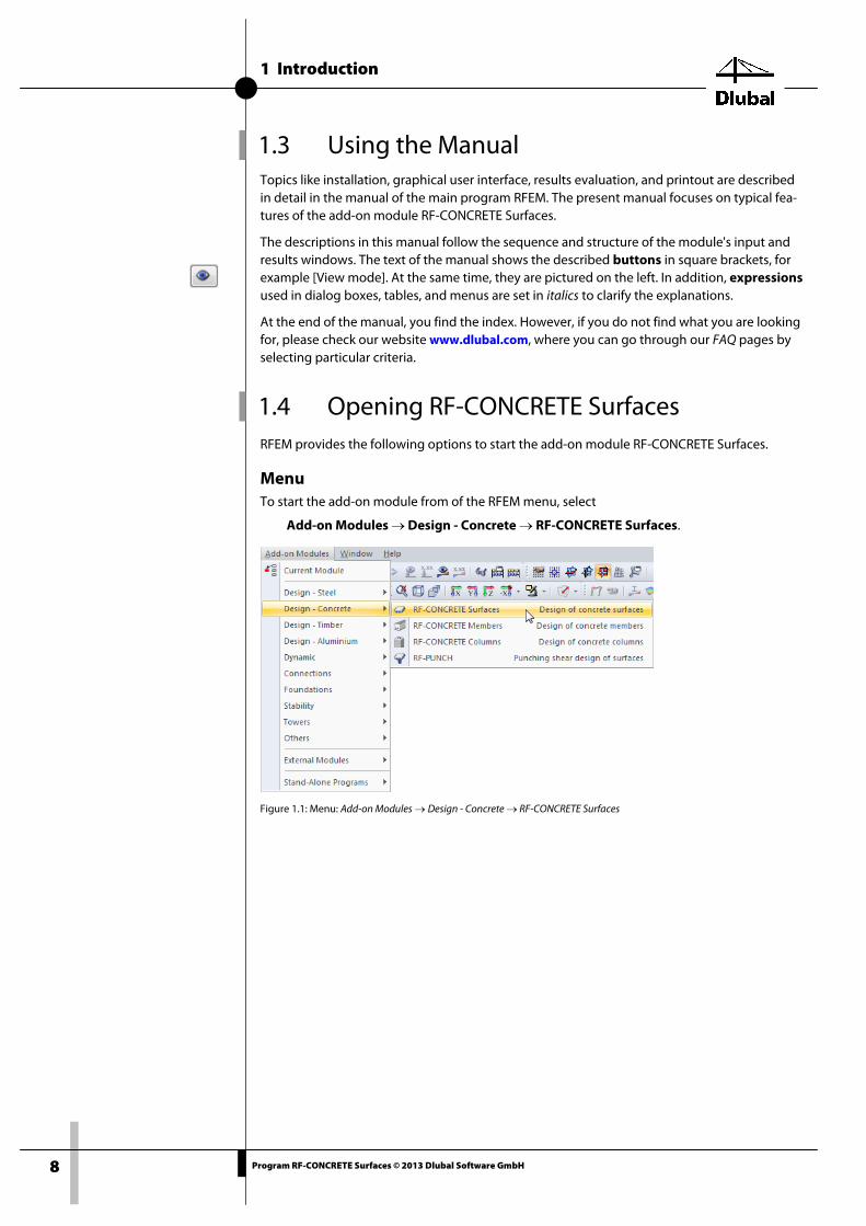
Menu To start the add-on module from of the RFEM menu, select
Add-on Modules → Design - Concrete → RF-CONCRETE Surfaces.
Figure 1.1: Menu: Add-on Modules → Design - Concrete → RF-CONCRETE Surfaces

1 Introduction
9 Program RF-CONCRETE Surfaces © 2013 Dlubal Software GmbH
Navigator Alternatively, you can open the add-on module in the Data navigator by clicking the entry
Add-on Modules → RF-CONCRETE Surfaces.
Figure 1.2: Data navigator: Add-on Modules → RF-CONCRETE Surfaces
Panel If results from RF-CONCRETE Surfaces are already available in the RFEM model, you can return to the design module by using the panel:
Set the relevant RF-CONCRETE Surfaces design case in the load case list, which is located in the menu bar. Click [Show Results] to display the reinforcements graphically.
The panel appears, showing the button [RF-CONCRETE Surfaces] which you can use to open the module.
Figure 1.3: Panel button [RF-CONCRETE Surfaces]

2 Theoretical Background
10 Program RF-CONCRETE Surfaces © 2013 Dlubal Software GmbH
2. Theoretical Background
2.1 Type of Model The Type of Model that you define when creating a new model has a crucial influence on how the structural components will be stressed.
Figure 2.1: Dialog box New Model - General Data, section Type of Model
If you select the model type 2D - XY (uZ/φX/φY), the plate will be subjected to bending only. The internal forces to be designed will be exclusively represented by moments whose vectors lie in the plane of the component.
If you select 2D - XZ (uX/uZ/φY) or 2D - XY (uX/uY/φZ), the wall (diaphragm) will be subjected only to compression or tension. The internal forces used for the design will be represented exclu-sively by axial forces whose vectors lie in the plane of the structural component.
In a spatial 3D type of model, both internal forces (moments and axial forces) are combined. Therefore, the structural component can be subjected to tension/compression and bending simultaneously. Thus, the internal forces to be designed are represented by axial forces as well as by moments whose vectors lie in the component's plane.

2 Theoretical Background
11 Program RF-CONCRETE Surfaces © 2013 Dlubal Software GmbH
2.2 Design of 1D and 2D Structural Components To check the ultimate limit state of a one-dimensional or a two-dimensional structural compo-nent consisting of reinforced concrete, it is always necessary to find a state of equilibrium be-tween the acting internal forces and resisting internal forces of the deformed component. In addition to this common feature in the ultimate limit state design of one-dimensional struc-tural components (members) and two-dimensional components (surfaces), there is also a cru-cial difference:
1D structural component (member) In a member, the acting internal force is always orientated in such a way that it can be com-pared to the resisting internal force that is determined from the design strengths of the mate-rials. As an example, we can take a member subjected to the axial compressive force N.
Figure 2.2: Design of a member
The dimensions of the structural component and the design value of the concrete strength can be used to determine the resisting compressive force. If it is smaller than the acting com-pressive force, the required area of the compressive reinforcement can be determined by means of the existing steel strain with an allowable concrete compressive strain.
2D structural component (surface) For a surface, the direction of the acting internal force is only in exceptional cases (trajectory reinforcement) orientated in such a way that the acting internal force can be set in relation to the resisting internal force: In an orthogonally reinforced wall, for example, the directions of the two principal axial forces n1 and n2 are usually not identical with the reinforcement direc-tions.
Figure 2.3: Design of a wall
Hence, for the dimensioning of the reinforcement of the reinforcement mesh, it is possible to use a procedure that is similar to the reinforcement of a member. The internal forces running in the reinforcement directions of the reinforcement mesh are required for the determination of the action-effects on concrete. These internal forces are termed design internal forces.

2 Theoretical Background
12 Program RF-CONCRETE Surfaces © 2013 Dlubal Software GmbH
To better understand the design internal forces, we can look at an element of a loaded rein-forcement mesh. For simplicity's sake, we assume the second principal axial force n2 to be zero.
Figure 2.4: Reinforcement mesh element with loading
The reinforcement mesh deforms under the given loading as follows.
Figure 2.5: Deformation of the reinforcement mesh element
The size of the deformation is limited by introducing a concrete compression strut to the rein-forcement mesh element.
Figure 2.6: Reinforcement mesh element with concrete compression strut
The concrete strut induces tensile forces in the reinforcement.
Figure 2.7: Tension forces in the reinforcement
These tensile forces in the reinforcement and the compressive force in the concrete are the design internal forces.

2 Theoretical Background
13 Program RF-CONCRETE Surfaces © 2013 Dlubal Software GmbH
Upon determination of the design internal forces, the design can be carried out like in a one-dimensional structural component.
Thus, the main feature of the design of a two-dimensional structural component is the trans-formation of the acting internal forces (principal internal forces) into design internal forces. The direction of the design internal forces allows for the dimensioning of the reinforcement and checking of the load-bearing capacity of concrete.
The following flowcharts illustrate the main difference between the design of one-dimensional and two-dimensional structural components.
One-dimensional structural component
Two-dimensional structural component
Determine the acting internal forces RE
RD ≥ RE
Satisfied Not satisfied
Determine the resisting internal forces RD
Determine the acting internal forces RE
Determine the design internal forces RB
RD ≥ RB
Satisfied Not satisfied
Determine the resisting internal forces RD

2 Theoretical Background
14 Program RF-CONCRETE Surfaces © 2013 Dlubal Software GmbH
2.3 Walls (Diaphragms)
2.3.1 Design Internal Forces The determination of design internal forces for walls is carried out according to BAUMANN'S [1] method of transformation. In this method, the equations for the determination of design in-ternal forces are derived for the general case of a reinforcement with three arbitrary directions. Then, these forces can be used for simpler cases like orthogonal reinforcement meshes with two reinforcement directions.
BAUMANN analyzed the equilibrium conditions with the following wall element.
Figure 2.8: Equilibrium conditions according to BAUMANN
Figure 2.8 shows a rectangular segment of a wall. It is subjected to the principal axial forces N1 and N2 (tensile forces). By means of factor k, the principal axial force N2 is expressed as a multi-ple of the principal axial force N1.
12 NkN ⋅=
Equation 2.1
Three reinforcement directions are applied in the wall. The reinforcement directions are signi-fied by x, y, and z. The clock-wise angle between the first principal axial force N1 and the direc-tion of the reinforcement direction x is signified by α. The angle between the first principal ax-ial force N and the reinforcement direction y is called β. The angle to the remaining reinforce-ment set is called γ.
BAUMANN writes in his thesis: If the shear and tension in the concrete is neglected, the external loading (N1, N2 = k · N1) of a wall element can usually be resisted by three internal forces orient-ed in any direction. In a reinforcement mesh with three reinforcement directions, these forces correspond to the three reinforcement directions (x), (y), and (z). Therese directions form with the greater main tensile force N1 the angles α, β, γ, and are called Zx, Zy, Zz (positive, because tensile forces).
To determine these forces Zx, Zy (and ZZ in case of a third reinforcement direction), we first de-fine a section parallel to the third reinforcement direction.

2 Theoretical Background
15 Program RF-CONCRETE Surfaces © 2013 Dlubal Software GmbH
Figure 2.9: Section parallel to the third reinforcement direction z
The value of the section length is taken as 1. With this section length, we determine the pro-jected section lengths running perpendicular to the respective force. In the case of the exter-nal forces, these are the projected section lengths b1 (perpendicular to force N1) and b2 (per-pendicular to force N2). In the case of the tension forces in the reinforcement, these are the projected section forces bx (perpendicular to tension force Zx) and by (perpendicular to tension force Zy).
The product of the respective force and the according projected section length yields the force that can be used to establish an equilibrium of forces.
Figure 2.10: Equilibrium of force in a section parallel to the reinforcement in the z-direction
The equilibrium between the external forces (N1, N2) and the internal forces (Zx, Zy) can thus be expressed as follows.
)cosbNsinbN()sin(
1bZ 2211xx β⋅⋅−β⋅⋅⋅
α−β=⋅
Equation 2.2
)cosbNsinbN()sin(
1bZ 2211yy α⋅⋅−α⋅⋅−⋅
α−β=⋅
Equation 2.3
To determine the equilibrium between the external forces (N1, N2) and the internal force Zz in the reinforcement direction z, we define a section parallel to the reinforcement direction x.

2 Theoretical Background
16 Program RF-CONCRETE Surfaces © 2013 Dlubal Software GmbH
Figure 2.11: Section parallel to the reinforcement direction x
Graphically, we can determine the following equilibrium.
Figure 2.12: Equilibrium of reinforcement in a section parallel to the reinforcement in x-direction
From the equilibrium between the external forces (N1, N2) and the internal forces (Zz, Zy), we can express Zz as follows.
)cosbNsinbN()ysin(
1bZ 2211zz β⋅⋅+β⋅⋅⋅
−β=⋅
Equation 2.4
For Zy, see equation 2.3.
If we replace the projected section lengths b1, b2, bx, by, bz by the values shown in the figure and use k as the quotient of the principal axial force N2 divided by N1, we obtain the following equations.
)sin()sin(coscosksinsin
N
Z
1
x
α−γ⋅α−βγ⋅β⋅+γ⋅β
=
Equation 2.5
)sin()sin(coscosksinsin
N
Z
1
y
γ−β⋅α−βγ⋅α⋅+γ⋅α
=
Equation 2.6
)sin()sin(coscosksinsin
N
Z
1
z
α−γ⋅γ−ββ⋅α⋅−β⋅α−
=
Equation 2.7
2 Theoretical Background
17 Program RF-CONCRETE Surfaces © 2013 Dlubal Software GmbH
These equations are at the core of the design algorithm for RF-CONCRETE Surfaces. Thus, we can determine from the acting internal forces N1 and N2 the design internal forces Zx, Zy, and Zz for the respective reinforcement directions.
By adding Equation 2.5, Equation 2.6, and Equation 2.7, we obtain:
k1NZ
N
Z
NZ
1
z
1
y
1
x +=++
Equation 2.8
By multiplying Equation 2.8 with N1 and substituting k with N2 / N1, we obtain the following equation that clarifies the equilibrium of the internal and external forces.
21zyx NNZZZ +=++
Equation 2.9
2.3.2 Two-Directional Reinforcement Meshes with k > 0 For a reinforcement with two reinforcement directions subjected to two positive principal axial forces N1 and N2, we select the direction of the concrete compressive strut as follows.
2β+α
=γ
Equation 2.10
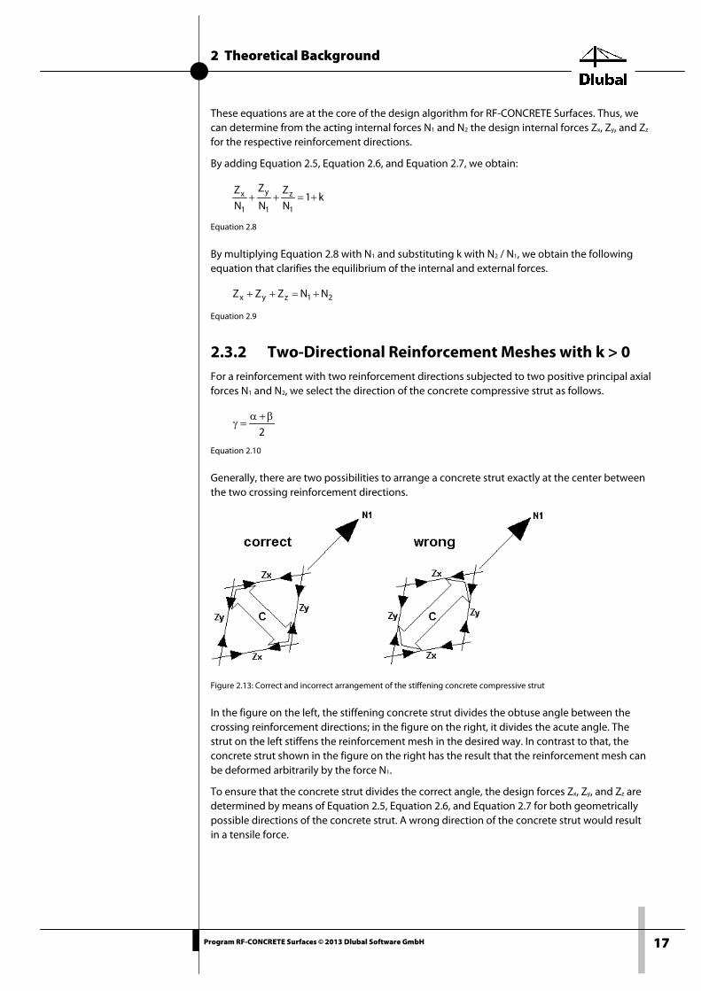
Generally, there are two possibilities to arrange a concrete strut exactly at the center between the two crossing reinforcement directions.
Figure 2.13: Correct and incorrect arrangement of the stiffening concrete compressive strut
In the figure on the left, the stiffening concrete strut divides the obtuse angle between the crossing reinforcement directions; in the figure on the right, it divides the acute angle. The strut on the left stiffens the reinforcement mesh in the desired way. In contrast to that, the concrete strut shown in the figure on the right has the result that the reinforcement mesh can be deformed arbitrarily by the force N1.
To ensure that the concrete strut divides the correct angle, the design forces Zx, Zy, and Zz are determined by means of Equation 2.5, Equation 2.6, and Equation 2.7 for both geometrically possible directions of the concrete strut. A wrong direction of the concrete strut would result in a tensile force.
2 Theoretical Background
18 Program RF-CONCRETE Surfaces © 2013 Dlubal Software GmbH
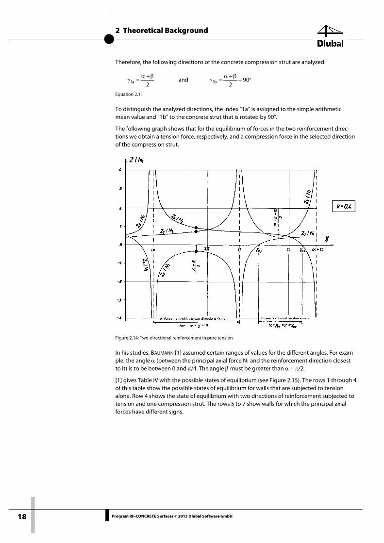
Therefore, the following directions of the concrete compression strut are analyzed.
2a1β+α
=γ and °+β+α
=γ 902b1
Equation 2.11
To distinguish the analyzed directions, the index "1a" is assigned to the simple arithmetic mean value and "1b" to the concrete strut that is rotated by 90°.
The following graph shows that for the equilibrium of forces in the two reinforcement direc-tions we obtain a tension force, respectively, and a compression force in the selected direction of the compression strut.
Figure 2.14: Two-directional reinforcement in pure tension
In his studies, BAUMANN [1] assumed certain ranges of values for the different angles. For exam-ple, the angle α (between the principal axial force N1 and the reinforcement direction closest to it) is to be between 0 and π/4. The angle β must be greater than α + π/2.
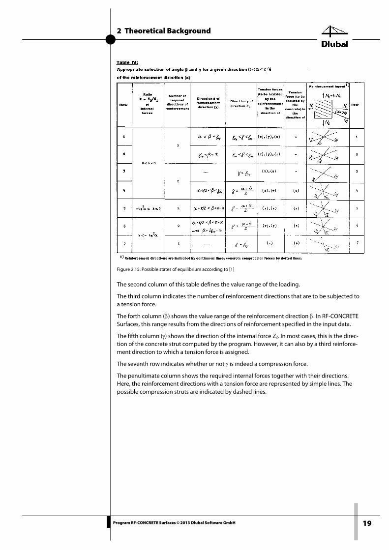
[1] gives Table IV with the possible states of equilibrium (see Figure 2.15). The rows 1 through 4 of this table show the possible states of equilibrium for walls that are subjected to tension alone. Row 4 shows the state of equilibrium with two directions of reinforcement subjected to tension and one compression strut. The rows 5 to 7 show walls for which the principal axial forces have different signs.
2 Theoretical Background
19 Program RF-CONCRETE Surfaces © 2013 Dlubal Software GmbH
Figure 2.15: Possible states of equilibrium according to [1]
The second column of this table defines the value range of the loading.
The third column indicates the number of reinforcement directions that are to be subjected to a tension force.
The forth column (β) shows the value range of the reinforcement direction β. In RF-CONCRETE Surfaces, this range results from the directions of reinforcement specified in the input data.
The fifth column (γ) shows the direction of the internal force ZZ. In most cases, this is the direc-tion of the concrete strut computed by the program. However, it can also by a third reinforce-ment direction to which a tension force is assigned.
The seventh row indicates whether or not γ is indeed a compression force.
The penultimate column shows the required internal forces together with their directions. Here, the reinforcement directions with a tension force are represented by simple lines. The possible compression struts are indicated by dashed lines.

2 Theoretical Background
20 Program RF-CONCRETE Surfaces © 2013 Dlubal Software GmbH
2.3.3 Two-Directional Reinforcement Meshes with k < 0 If in a two-directional reinforcement mesh, the main axial forces N1 and N2 have different signs, for the equilibrium of forces this results in a tension force in the two reinforcement directions, respectively, and a compression forces in the direction of the compressive strut.
Figure 2.16: Two-directional reinforcement in tension and compression
Rows 5 and 6 of Table IV (Figure 2.15) give examples for this possible state of equilibrium.
For a wall subjected to tension as well as compression, however, it can happen that for the selected direction of the concrete strut (arithmetic mean between the two directions of rein-forcement) a compression strut is obtained, as expected, in a direction γ and in a further direc-tion β. This is the case if the arithmetic mean is to the left of the zero-crossing of the force dis-tribution of Zy in the diagram above. However, this kind of equilibrium is not possible. We de-termine the reinforcement of the conjugated direction, that is, the value γ0y is used for the con-crete strut direction γ.
α⋅−=γ cotktan y0
Equation 2.12
This means that no force occurs in the second reinforcement direction y under the angle β. Row 7 in Table IV (Figure 2.15) shows an example for this equilibrium of forces. In the add-on module RF-CONCRETE Surfaces, such a case of equilibrium is represented if a compression force in the direction of the reinforcement direction y is obtained for the routinely assumed direction of the concrete strut (arithmetic mean between the directions of the two reinforce-ment directions).
Thus, we have described all possible states of equilibrium for two-directional reinforcements.

2 Theoretical Background
21 Program RF-CONCRETE Surfaces © 2013 Dlubal Software GmbH
2.3.4 Possible Load Situations The load is obtained by applying the principal axial forces n1 and n2, with the principal axial force n1 under consideration of the sign always being greater than the principal axial force n2.
Figure 2.17: Mohr's circle
Different load situations are distinguished, depending on the sign of the principal axial forces.
Figure 2.18: Load situations

2 Theoretical Background
22 Program RF-CONCRETE Surfaces © 2013 Dlubal Software GmbH
In a matrix of principal axial force, we obtain the following designations of the individual de-sign situations (n1 is called here nI, n2 is called nII):
Figure 2.19: Matrix of principal axial force for load situations
The determination of design axial forces by means of Equation 2.5 through Equation 2.7 is de-scribed in the previous chapters for the load situations Elliptical Tension and Hyperbolic State. For the load situation Parabolic Tension, the design axial forces are obtained by using the same formulas. The value k is to be taken as zero in Equation 2.5 through Equation 2.7.
Now we will explain the design axial forces for the following design situations.
Elliptical compression in a mesh with three reinforcement directions Equation 2.5 through Equation 2.7 are applied without changes, even if the two principal axial forces n1 and n2 are negative. If a negative design axial force results for each of the three rein-forcement directions, none of the three provided reinforcement directions is activated. The concrete can transfer the principal axial forces by itself, that is, without the use of a reinforce-ment mesh in tension, stiffened by a concrete strut.
The assumption about the introduction of concrete compression forces in the direction of the provided reinforcement to resist the principal axial forces is purely hypothetical. It is based on the wish to obtain a distribution of the principal compression forces in the direction of the in-dividual reinforcement directions in order to be able to determine the minimum compression reinforcement that is required, for example, by EN 1992-1-1, clause 9.2.1.1. To this end, a stati-cally required concrete cross-section is necessary. It can only be determined by means of the previously determined concrete compression forces in the direction of the provided rein-forcement.
In the determination of the minimum compressive reinforcement, other standards do without a statically required concrete cross-section resulting from the transformed principal axial force into a design axial force. However, for a unified transformation method across different stand-ards, the principal compressive forces are transformed in the defined reinforcement directions for these standards, too. Studies have shown that the design with transformed compressive forces is on the safe side. The concrete pressures occurring in the direction of the individual re-inforcement directions are verified.
However, if after the transformation at least one of the design axial forces is positive, the rein-forcement mesh is activated for this load situation. Then, as described in chapter 2.3.2 and 2.3.3, an internal equilibrium of forces in the form of two reinforcement directions and one selected concrete compression strut is to be established.
2 Theoretical Background
23 Program RF-CONCRETE Surfaces © 2013 Dlubal Software GmbH
Elliptical compression in a two-directional mesh Equation 2.5 through Equation 2.7 are used without changes. If the direction of the two main axial forces is identical to the direction of both reinforcement directions, the design axial forces are equal to the principal axial forces.
If the principal axial forces deviate from the reinforcement directions, the equilibrium between a compression strut in the concrete and the design axial forces in the reinforcement directions is searched for again. For the two directions of the concrete strut, the two intermediate angles between the reinforcement directions are reanalyzed. The same applies as for the elliptical tension: The assumption of a concrete strut direction is assumed to be correct if a negative de-sign force is indeed assigned to the concrete strut. If allowable solutions are obtained for both concrete strut directions, the smallest absolute value of all design axial forces decides which solution is chosen.
If the design axial force for a reinforcement direction is a compressive force, the program first checks whether the concrete can resist this design axial force. If this is not the case, the pro-gram determines a compression reinforcement ratio.
Parabolic compression in a two-directional mesh In this load situation, the principal axial force n1 is zero. Since the quotient k = n2 / n1 cannot be calculated anymore, we cannot use Equation 2.5 through Equation 2.7 as usually. The follow-ing modifications are necessary.
)sin()sin(
coscosnsinsinnn 21
α−γ⋅α−βγ⋅β⋅+γ⋅β⋅
=α
)sin()sin(
coscosnsinsinnn 21
γ−β⋅α−βγ⋅α⋅+γ⋅α⋅
=β
)sin()sin(
coscosnsinsinnn 21
α−γ⋅γ−ββ⋅α⋅+β⋅α⋅−
=γ
Equation 2.13
With the modified equations, the program search for the design axial forces in the two rein-forcement directions and one design axial force for the concrete. If one reinforcement direc-tion is identical to the acting principal axial force, then its design axial force is the principal axi-al force. Otherwise, solutions with one concrete strut between the two reinforcement direc-tions are obtained.
Parabolic compression in a three-directional mesh The formulas presented above are used according to Equation 2.13.
If the principal axial force runs in a reinforcement direction, solutions (like for the parabolic tension) for a concrete strut direction between the first and the second reinforcement direc-tion or the first and third reinforcement direction are analyzed. Again, the smallest absolute value of all design axial forces values decides which solution is chosen.

2 Theoretical Background
24 Program RF-CONCRETE Surfaces © 2013 Dlubal Software GmbH
2.3.5 Design of the Concrete Compression Strut The concrete compression force in the selected direction of the concrete strut is one of the de-sign forces. It is analyzed whether or not the concrete can resist the compression force. How-ever, we do not apply the complete compression stress fcd. Instead, the allowable concrete compression stress is reduced to 80%, thus following the sense of the recommendation by SCHLAICH/SCHÄFER ([13], page 373).
With the reduced concrete compression stress fcd,08, the magnitude of the resisting axial force nstrut,d is determined per meter. This is done by multiplying the concrete compression stress by the width of one meter and the wall thickness.
dbfn 08,cdd,strut ⋅⋅=
Equation 2.14
This resisting concrete compression force can now be compared to the acting concrete com-pression force nstrut. The analysis of the concrete compression strut is OK, if
strutd,strut nn ≥
Equation 2.15
The design of the concrete compression strut is carried out in the same way for all standards – of course, with the respective valid material properties.
2.3.6 Determination of Required Reinforcement To determine the dimension of the reinforcement area to be used, the resisting design axial force nϕ in the respective reinforcement direction ϕ is divided by the reinforcing steel strength.
Depending on the standard and concrete strength class, the steel stress at yield is defined dif-ferently. For the design, the respective partial safety factor for the reinforcing steel has to be considered.
If the reinforcement is in compressive strain instead of tension, the steel stress for the allowa-ble concrete compression at failure shall be determined. It is the same in all standards and equals 2 ‰. Thus, the steel stress can be determined by using the modulus of elasticity as fol-lows:
002.0Es ⋅=σ
Equation 2.16
If the steel stress is greater than the steel stress at yielding, the steel stress at yielding is used. However, a compression reinforcement is determined only in the case if the resistant axial force nstrut,d per meter of the concrete is smaller than the acting, compression-inducing design axial force. The compression reinforcement is then designed for the difference of the two axial forces.

2 Theoretical Background
25 Program RF-CONCRETE Surfaces © 2013 Dlubal Software GmbH
2.3.7 Reinforcement Rules
All standards contain regulations for plate structures regarding size and direction of the rein-forcement to be used. To this purpose, the standard classifies the plate structures in certain structural elements. For example, EN 1992-1-1 distinguishes the following elements of struc-tures:
• Plate (slab)
• Wall (diaphragm)
• Deep beam
The following graphic illustrates the relation between the user-defined Type of Model, the model for the design, and the element of structure according to the standard, which is used to determine the size and direction of the minimum or maximum reinforcement.
Figure 2.20: Relation between type of model, design model, and structural element
If 3D (see Figure 2.1, page 10) is selected as type of model, the structural component is always designed as shell – independent of whether both axial forces and moments occur in portions of the structural component or if there is only one of these internal forces or moments. A type of model defined as 2D - XY (uZ/φX/φY) is always designed as plate, the two types 2D - XZ (uX/uZ/φY) and 2D - XY (uX/uY/φZ) are designed as walls.
After selecting the structural element, the rules of the respective standard are automatically used in the determination of the required reinforcement. We will now briefly look at these rules acc. to EN 1992-1-1. The standard distinguishes between solid plates, walls, and deep beams.
Solid plates
For solid plates, EN 1992-1-1 specifies the following:
• Clause 9.2.1.1 (1): The area of longitudinal tension reinforcement should not be taken as less than As,min.
db0013.0dbf
f26.0A tt
yk
ctmmin,s ⋅⋅≥⋅⋅⋅=
Equation 2.17
• Clause 9.2.1.1 (3): The cross-sectional area of tension or compression reinforcement should not exceed As,max outside lap locations. The recommended value is 0.04 Ac.
According to DIN EN 1992-1-1/NA:2010, the sum of the tension and compression reinforce-ment may not exceed As,max = 0.08 Ac. This is also true for the lap locations.

2 Theoretical Background
26 Program RF-CONCRETE Surfaces © 2013 Dlubal Software GmbH
Walls
For walls, EN 1992-1-1 specifies the following:
• Clause 9.6.2 (1): The area of the vertical reinforcement should lie between As,vmin and As,vmax. The recommended values are As,vmin = 0.002 Ac and As,vmax = 0.04 Ac outside lap locations.
DIN EN 1992-1-1/NA:2010 specifies
- General: As,vmin = 0.15|NEd| / fyd ≥ 0.0015 Ac
- As,vmax = 0.04 Ac (this value may be doubled at laps)
The percentage of reinforcement should be equal at both wall faces.
• Clause 9.6.3 (1): Horizontal reinforcement running parallel to the faces of the wall (and to the free edges) should be provided at the outer face. It should not be less than As,hmin. The recommended value is either 25 % of the vertical reinforcement or 0.001 Ac.
DIN EN 1992-1-1/NA:2010 specifies
- General: As,hmin = 0.20 As,v
The diameter of the horizontal reinforcement should not be less than one quarter of the diameter of the perpendicular members.
Deep beam
According to EN 1992-1-1, clause 5.3.1 (3), a beam is considered as a deep beam if the span is less than three times the cross-section depth. If this is the case, the following applies:
• Clause 9.7 (1): Deep beams should normally be provided with an orthogonal reinforce-ment mesh near each face, with a minimum of As,dbmin . The recommended value is 0.1% but not less than 150 mm2/m in each face and each direction.
DIN EN 1992-1-1/NA:2010 specifies
- As,dbmin = 0.075 % von Ac ≥ 150 mm2/m

2 Theoretical Background
27 Program RF-CONCRETE Surfaces © 2013 Dlubal Software GmbH
User-defined, cross-standard rules of reinforcement detailing
In addition to the normative requirements (that means they cannot be modified) of reinforce-ment detailing, there is the possibility to specify user-defined rules. The minimum reinforce-ments can be specified in the Reinforcement Ratios tab of the 1.4 Reinforcement window.
Figure 2.21: Window 1.4 Reinforcement, tab Reinforcement Ratios
If, for example, you specify a minimum secondary reinforcement of 20 % of the greatest placed longitudinal reinforcement, the [Calculation] determines the maximum longitudinal reinforce-ment first. In the results windows, this is shown as Required Reinforcement.
Figure 2.22: Required longitudinal reinforcement and button [Design Details]
To check the minimum secondary reinforcement, click [Design Details].
2 Theoretical Background
28 Program RF-CONCRETE Surfaces © 2013 Dlubal Software GmbH
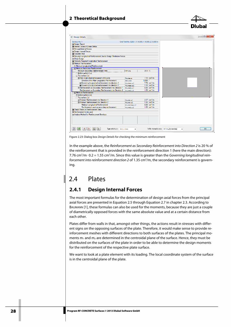
Figure 2.23: Dialog box Design Details for checking the minimum reinforcement
In the example above, the Reinforcement as Secondary Reinforcement into Direction 2 is 20 % of the reinforcement that is provided in the reinforcement direction 1 (here the main direction): 7.76 cm2/m · 0.2 = 1.55 cm2/m. Since this value is greater than the Governing longitudinal rein-forcement into reinforcement direction 2 of 1.35 cm2/m, the secondary reinforcement is govern-ing.
2.4 Plates
2.4.1 Design Internal Forces The most important formulas for the determination of design axial forces from the principal axial forces are presented in Equation 2.5 through Equation 2.7 in chapter 2.3. According to BAUMANN [1], these formulas can also be used for the moments, because they are just a couple of diametrically opposed forces with the same absolute value and at a certain distance from each other.
Plates differ from walls in that, amongst other things, the actions result in stresses with differ-ent signs on the opposing surfaces of the plate. Therefore, it would make sense to provide re-inforcement meshes with different directions to both surfaces of the plates. The principal mo-ments m1 and m2 are determined in the centroidal plane of the surface. Hence, they must be distributed on the surfaces of the plate in order to be able to determine the design moments for the reinforcement of the respective plate surface.
We want to look at a plate element with its loading. The local coordinate system of the surface is in the centroidal plane of the plate.

2 Theoretical Background
29 Program RF-CONCRETE Surfaces © 2013 Dlubal Software GmbH
Figure 2.24: Plate element with local surface coordinate system in the centroidal plane of the plate
In RFEM, the bottom surface is always in the direction of the positive local surface axis z. Ac-cordingly, the top surface is defined in the direction of the negative local z-axis. The surface axes can be switched on in the Display navigator by selecting
Model → Surfaces → Surface Axis Systems x,y,z.
Alternatively, you can use the context menu (see Figure 3.29, page 150).
The principal moments m1 and m2 are determined in RFEM for the centroidal plane of the plate.
Figure 2.25: Principal moments m1 and m2 in the centroidal plane of the plate
The principal moments are indicated by simple arrows. They are oriented like the reinforce-ment that would be required for resisting them. To obtain design moments from these prin-cipal moments for the reinforcement mesh at the bottom surface of the plate, the principal moments are shifted to the bottom surface of the plate without being changed. For the de-sign, they are signified by the Roman indexes mI and mII.
Figure 2.26: Principal moments shifted to bottom surface of the plate
To obtain the principal moments for determining the design moments for the reinforcement mesh at the top surface of the plate, the principal moments are shifted to the top surface of the plate. In addition, their direction is rotated by 180°.
Figure 2.27: Principal moments shifted to top surface of plate
Top and Bottom surface

2 Theoretical Background
30 Program RF-CONCRETE Surfaces © 2013 Dlubal Software GmbH
The principal moment is usually denoted m1, which, considering the ,s greater (see Figure 2.17, page 21). Hence, the denotations of the principal moments at the top surface of the plate must be reversed.
Thus, the principal moments for determining the design moments at both plate surfaces are as follows:
Figure 2.28: Final principal moments at bottom and top surface of the plate
If the principal moments for both plate surfaces are known, the design moments can be de-termined. To this end, the first step is to determine of the differential angle of the reinforce-ment directions to the direction of the principal moment at each plate surface.
The smallest differential angle specifies the positive direction. All other angles are determined in this positive direction, and then sorted by their size. In RF-CONCRETE Surfaces, they are de-noted as αm,+z, βm,+z, and γm,+z (see the following example). The index +z indicates the bottom surface.
Figure 2.29: Differential angle according to [1] for bottom surface of plate (here, for three directions of reinforcement)
Then, Equation 2.5 through Equation 2.7 according to BAUMANN [1] are used in order to deter-mine the design moments:
)sin()sin(coscosksinsin
mm I α−γ⋅α−βγ⋅β⋅+γ⋅β
⋅=α
)sin()sin(coscosksinsin
mm I γ−β⋅α−βγ⋅α⋅+γ⋅α
⋅=β
)sin()sin(coscosksinsin
mm I α−γ⋅γ−ββ⋅α⋅+β⋅α−
⋅=γ
Equation 2.18
2 Theoretical Background
31 Program RF-CONCRETE Surfaces © 2013 Dlubal Software GmbH
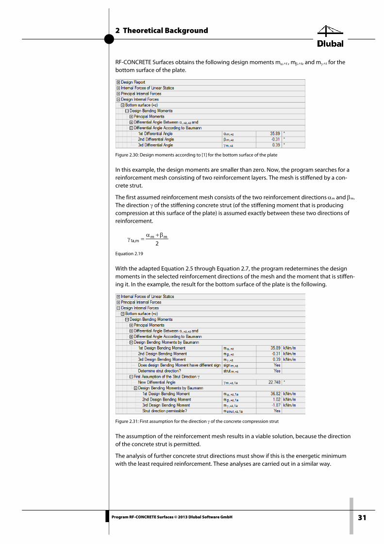
RF-CONCRETE Surfaces obtains the following design moments mα,+z , mβ,+z, and mγ,+z for the bottom surface of the plate.
Figure 2.30: Design moments according to [1] for the bottom surface of the plate
In this example, the design moments are smaller than zero. Now, the program searches for a reinforcement mesh consisting of two reinforcement layers. The mesh is stiffened by a con-crete strut.
The first assumed reinforcement mesh consists of the two reinforcement directions αm and βm. The direction γ of the stiffening concrete strut (of the stiffening moment that is producing compression at this surface of the plate) is assumed exactly between these two directions of reinforcement.
2mm
m,a1β+α
=γ
Equation 2.19
With the adapted Equation 2.5 through Equation 2.7, the program redetermines the design moments in the selected reinforcement directions of the mesh and the moment that is stiffen-ing it. In the example, the result for the bottom surface of the plate is the following.
Figure 2.31: First assumption for the direction γ of the concrete compression strut
The assumption of the reinforcement mesh results in a viable solution, because the direction of the concrete strut is permitted.
The analysis of further concrete strut directions must show if this is the energetic minimum with the least required reinforcement. These analyses are carried out in a similar way.

2 Theoretical Background
32 Program RF-CONCRETE Surfaces © 2013 Dlubal Software GmbH
Once all sensible possibilities for a reinforcement mesh consisting of two reinforcement direc-tions and a stiffening concrete strut have been analyzed, the sums of the absolute design mo-ments are shown. For the example above, the overview looks as follows.
Figure 2.32: Sum of the absolute design moments
The Smallest Energy for all Valid Cases is given by Σmin,+z as minimum absolute sum of the de-termined design moments. In the example, the reinforcement mesh from the reinforcement directions for the differential angle βm,+z,2a yields the most favorable solution for the bottom surface of the plate.
The design details also show the direction of the governing concrete strut. This direction is related to the definition of the differential angles according to BAUMANN. Hence, the program also gives the direction Φstrut related to the direction of the reinforcement. In the example, the following angle of the concrete strut is determined for the bottom surface of the plate.
Figure 2.33: Governing concrete compression strut
For an optimized direction of the design moment stiffening the reinforcement mesh (see Fig-ure 3.40, page 159), we obtain the design moments according to BAUMANN. As shown in the following figure, these design moments are applied to the defined reinforcement directions.

2 Theoretical Background
33 Program RF-CONCRETE Surfaces © 2013 Dlubal Software GmbH
Figure 2.34: Final design moments for bottom surface of plate
2.4.2 Design of Stiffening Moment After determining the design moments, the program analyzes the compression struts. It checks if the moments for the stiffening of the reinforcement mesh can be resisted by the plate.
This check is shown in the Concrete Strut entry:
Figure 2.35: Analysis of the stiffening moment
The program performs a normal bending design for the determined moments at the bottom and top surface of the plate. However, this design does not aim at finding a reinforcement: The aim is rather to verify that the compression zone of concrete can yield a resulting compressive force. Multiplied by the lever arm of the internal forces, it results in a greater moment on the side of the resistance than the acting moment.

2 Theoretical Background
34 Program RF-CONCRETE Surfaces © 2013 Dlubal Software GmbH
The analysis is not verified if the moment on the side of the resistance is smaller than the gov-erning design moment nsstrut even in the case of a maximum allowable bending compressive strain of the concrete and a maximum allowable retraction of an assumed reinforcement.
The current standards regulate the satisfaction of the allowable strain via the limit of the ratio between neutral axis depth x and effective depth d. For this, the stress-strain relationships for concrete and reinforcing steel as well as the limit strains of these standards are used (see the following explanations for EN 1992-1-1).
Stress-strain relationships for cross-section design The parabola-rectangle diagram according to Figure 3.3 of EN 1992-1-1 is used as the calcula-tion value of the stress-strain relation.
Figure 2.36: Stress-strain diagram for concrete under compression
The stress-strain diagram of the reinforcing steel is shown in Figure 3.8 of EN 1992-1-1.
Figure 2.37: Stress-strain relation for reinforcing steel

2 Theoretical Background
35 Program RF-CONCRETE Surfaces © 2013 Dlubal Software GmbH
The allowable limit deformations are shown in Figure 6.1 of EN 1992-1-1.
Figure 2.38: Possible strain distributions in the ultimate limit state
The ultimate limit state is determined by means of the limit strains. Either the concrete or the reinforcing steel fails, depending on where the limit strain occurs.
• Failure of concrete, for example, C30/37:
Limit strain in case of axial compression: εc2 = -2.0 ‰
Ultimate strain: εcu2 = -3.5 ‰
• Failure of reinforcing steel, for example B 500 S (A):
Steel strain under maximum load: εuk = 25 ‰
• Simultaneous failure of concrete and reinforcing steel:
The limit compressive strains of concrete and steel occur simultaneously.
2 Theoretical Background
36 Program RF-CONCRETE Surfaces © 2013 Dlubal Software GmbH
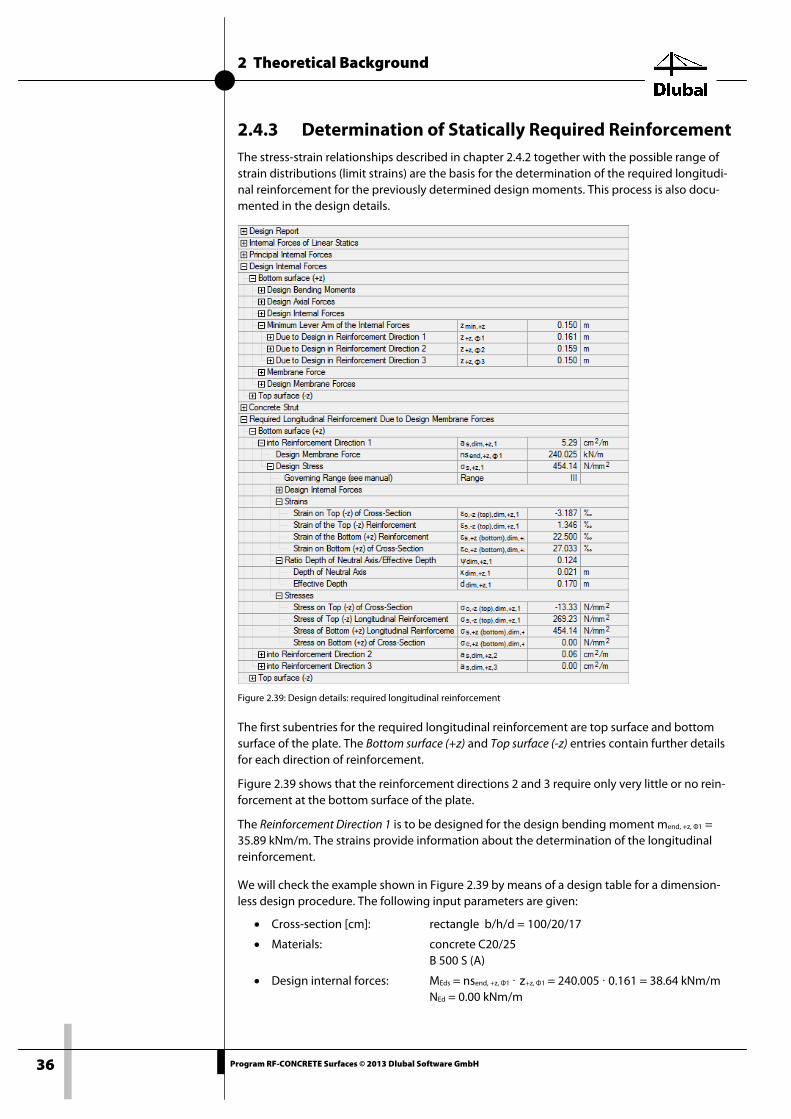
2.4.3 Determination of Statically Required Reinforcement The stress-strain relationships described in chapter 2.4.2 together with the possible range of strain distributions (limit strains) are the basis for the determination of the required longitudi-nal reinforcement for the previously determined design moments. This process is also docu-mented in the design details.
Figure 2.39: Design details: required longitudinal reinforcement
The first subentries for the required longitudinal reinforcement are top surface and bottom surface of the plate. The Bottom surface (+z) and Top surface (-z) entries contain further details for each direction of reinforcement.
Figure 2.39 shows that the reinforcement directions 2 and 3 require only very little or no rein-forcement at the bottom surface of the plate.
The Reinforcement Direction 1 is to be designed for the design bending moment mend, +z, Φ1 = 35.89 kNm/m. The strains provide information about the determination of the longitudinal reinforcement.
We will check the example shown in Figure 2.39 by means of a design table for a dimension-less design procedure. The following input parameters are given:
• Cross-section [cm]: rectangle b/h/d = 100/20/17
• Materials: concrete C20/25 B 500 S (A)
• Design internal forces: MEds = nsend, +z, Φ1 · z+z, Φ1 = 240.005 · 0.161 = 38.64 kNm/m NEd = 0.00 kNm/m

2 Theoretical Background
37 Program RF-CONCRETE Surfaces © 2013 Dlubal Software GmbH
2
c
ckcd cm/kN13.1
5.10.285.0f
f =⋅
=γ⋅α
=
1183.013.117100
3864
fdb
M2
cd2Eds
Eds =⋅⋅
=⋅⋅
=µ
For µEds = 0.1183, it is possible to interpolate the following values from the design tables (for example [7] Annex A4):
( ) ( )1265.0
11.012.0
11.01183.01170.01285.01170.01 =
−−⋅−
+=ω
( ) ( ) 2sd cm/kN37.45
11.012.011.01183.024.4540.45
24.45 =−
−⋅−+=σ
With these values, it is possible to determine the required longitudinal reinforcement:
m/cm36.537.45
013.1171001265.0NfdbA 2
sd
Edcd11s =
+⋅⋅⋅=
σ+⋅⋅⋅ω
=
2.4.4 Shear Design
The shear design differs among the individual standards significantly. In the following, it is de-scribed for EN 1992-1-1.
The check of shear force resistance is only to be performed in the ultimate limit state (ULS). The actions and resistances are considered with their design values. The general check requirement is the following:
VEd ≤ VRd
Equation 2.20
where
VEd design value of applied shear force (principal shear force determined by RF-CONCRETE Surfaces)
VRd design value of shear force resistance
Depending on the failure mechanism, the design value of the shear force resistance is deter-mined by one of the following three values:
VRd,c design shear resistance of a structural component without shear reinforcement
VRd,s design shear resistance of a structural component with shear reinforcement; limitation of the resistance by failure of shear reinforcement (failure of tie)
VRd,max design value of the maximum shear force which can be sustained by the member, limited by crushing of the compression struts
If the applied shear force VEd remains below the value of VRd,c, then no calculated shear rein-forcement is necessary and the check is verified.
If the applied shear force VEd is higher than the value of VRd,c, a shear reinforcement must be designed. The shear reinforcement must resist the entire shear force. In addition, the bearing capacity of the concrete compression strut must be analyzed.
VEd ≤ VRd,s
VEd ≤ VRd,max
Equation 2.21
2 Theoretical Background
38 Program RF-CONCRETE Surfaces © 2013 Dlubal Software GmbH
2.4.4.1 Design Shear Resistance Without Shear Reinforcement
VRd,c = [CRd,c · k · (100 · ρ1 · fck )1/3 + k1 · σcp] · bw · d (6.2a)
Equation 2.22
where
CRd,c = 0.18 / γc (recommended value; acc. to DIN EN 1992-1-1/NA:2010: CRd,c = 0.15 / γc)
k = 1 + √(200 / d) ≤ 2.0 Scaling factor for considering the plate thickness
d Mean effective depth in [mm]
ρ1 = Asl / (bw · d) ≤ 0.02 Longitudinal reinforcement ratio
Asl Area of tensile reinforcement which extends at least by d be-yond the considered cross-section and is effectively an-chored there
fck Characteristic value of concrete compressive strength in [N/mm2]
bw Cross-section width
d Effective depth of bending reinforcement in [mm]
σcp = NEd / Ac < 0.2 · fcd Design value of concrete longitudinal stress in [N/mm2]
NEd Applied axial force in direction of principal shear force
You may apply the following minimum value of the shear force resistance VRd,c,min:
VRd,c = ( νmin + k1 · σcp ) · bw · d (6.2b)
Equation 2.23
where
k1 = 0.15 (recommended value; acc. to DIN EN 1992-1-1/NA:2010: k1 = 0.12)
νmin = 0.035 · k3/2 · fck1/2 (recommended value) (6.3N)
according to DIN EN 1992-1-1/NA:2010:
νmin = (0.0525 / γc) · k3/2 · fck1/2 for d ≤ 600mm (6.3aDE)
νmin = (0.0375 / γc) · k3/2 · fck1/2 for d > 800mm (6.3bDE)
for 600 mm < d ≤ 800 mm interpolation possible
These equations are mostly intended for the one-dimensional design case (beam). There is on-ly one provided longitudinal reinforcement from which the ratio of the longitudinal reiforce-ment is determined. For two-dimensional structural components with up to three reinforce-ment directions, it is not so easy to say how great the longitudinal reinforcement to be applied is.

2 Theoretical Background
39 Program RF-CONCRETE Surfaces © 2013 Dlubal Software GmbH
The Longitudinal Reinforcement tab of the 1.4 Reinforcement window offers three possibilities to specify the provided longitudinal reinforcement for the shear force check.
Figure 2.40: Window 1.4 Reinforcement, tab Longitudinal Reinforcement
Apply required longitudinal reinforcement First, the program analyzes which reinforcement direction at the two surfaces of the plate after the design, including an applied tension force according to clause 6.2.3 (7), are subjected to tension. According to EN 1992-1-1, the provided ratio of longitudinal reinforcement can be de-termined only from the area of the provided tensile reinforcement.
In order to transform the reinforcement from the different reinforcement directions with ten-sile forces in direction β of the maximum shear force, the direction of the maximum shear force is determined as follows.
x
y
v
varctan=β
Equation 2.24
With this, the program determines the differential angle δφi between the respective reinforce-ment direction ϕi and the direction of the maximum shear force.
ii ϕ−β=δϕ
Equation 2.25
With the differential angle δϕi, it is possible to determine the component asl,i of a certain ten-sioned longitudinal reinforcement as,i.
( )i2
i,si,sl cosaa δϕ⋅=
Equation 2.26
In Equation 2.22, the tensile reinforcement asl to be applied for the determination of VRd,c is the sum of the components from the individual reinforcement directions to which tension is as-signed.
( )∑ δϕ⋅= i2
i,ssl cosaa
Equation 2.27
2 Theoretical Background
40 Program RF-CONCRETE Surfaces © 2013 Dlubal Software GmbH
Apply the greater value resulting from either required or provided rein-forcement (basic and add. reinforcement) per reinforcement direction The second option shown in Figure 2.40 on page 39 is used to determine the required tension reinforcement asl as described above. First, the program checks if a tension force is assigned to the required longitudinal reinforcement. The provided longitudinal reinforcement asl is then determined according to Equation 2.26 and Equation 2.27.
Then, the design shear resistance VRd,c without shear reinforcement is determined. It might turn out that the check of shear force is possible without shear reinforcement. If the shear rein-forcement VRd,ct is negative and not sufficient, it is analyzed whether for a reinforcement direc-tion the statically required longitudinal reinforcement as,dim or the user-defined basic rein-forcement as,def is the greater reinforcement as,max.
With this greater reinforcement as,max, the provided longitudinal reinforcement asl is redeter-mined according to Equation 2.26 and Equation 2.27. Then, the shear resistance VRd,c without shear reinforcement is redetermined.
If it turns out that the shear resistance VRd,c without shear reinforcement and the respectively greater reinforcement (either the statically required or user-defined longitudinal reinforce-ment) is sufficient, the shear force check is satisfied. If despite this longitudinal reinforcement, the cross-section still cannot be designed because it is fully cracked, an according message appears.
If despite the application of the greater longitudinal reinforcement (statically required or user-defined longitudinal reinforcement) cannot be avoided, the shear resistance VRd,c is redeter-mined with the statically required longitudinal reinforcement It would not make much sense to apply the user-defined longitudinal reinforcement, and thus output it later than required, if by applying it a shear reinforcement cannot be avoided after all.
The shear force design comprises the check of the shear strength VRd,max of the concrete strut and the design shear resistance VRd,s of the shear reinforcement, as well as the determination of the required shear reinforcement.
Automatically increase longitudinal reinforcement to avoid shear reinforcement In the thired option (see Figure 2.40), the Equation 2.22 for VRd,c is solved for the longitudinal reinforcement ratio ρ1. VRd,c is taken as the applied shear force VEd.
ck
3
1
cdc
1w
cEd
l f100
15.0
12.0
15.0bd
V
⋅
η⋅κ⋅σ⋅γ⋅
+η⋅κ⋅⋅⋅
γ⋅
=ρ
Equation 2.28
Thus, if the longitudinal reinforcement ratio is high enough, it becomes possible to do without shear reinforcement.
First, RF-CONCRETE Surfaces checks again the design shear resistance VRd,c with the statically required longitudinal reinforcement. If this first design shear resistance is not enough, the lon-gitudinal reinforcement asl is increased in the direction of the principal shear force. The longi-tudinal reinforcement asl cannot be increased arbitrarily.
The flowchart on the following page shows the cases in which shear reinforcement can be avoided and in which a shear reinforcement must be used with the statically required longitu-dinal reinforcement from the design.

2 Theoretical Background
41 Program RF-CONCRETE Surfaces © 2013 Dlubal Software GmbH
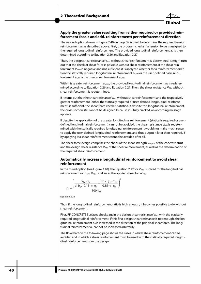
Figure 2.41: Flowchart for increase of longitudinal reinforcement to avoid shear reinforcement
The two paths on the left (VRd,c ≥ 0, VRd,c < 0) indicate that the shear reinforcement is successfully avoided. The second path represents the possibility that even if the longitudinal reinforcement is increased, the design shear resistance VRd,c remains negative, and therefore no check of shear force is possible for the fully cracked cross-section.
The other four paths (VRd,c < VEd , ρ > ρmax , no tension reinforcement, tension reinforcement 90°) show the reasons why it is not possible to increase the longitudinal reinforcement. For exam-ple, despite the maximum longitudinal reinforcement ratio, shear reinforcement is unavoida-ble or the allowed longitudinal reinforcement ratio of the individual directions of reinforce-ment is exceeded. When the longitudinal reinforcement asl that is increased in the principal di-rection of the principal shear force is distributed to the individual directions of reinforcement, the program checks for each of these reinforcement directions if the user-defined longitudinal reinforcement ratio is not exceeded. If this is not the case, the longitudinal reinforcement ratio ρl is determined by using the option Apply required longitudinal reinforcement.
To better understand the two right paths, we must look at the longitudinal reinforcement in-creased in the direction of the principal shear force and distributed to the individual directions of reinforcement. If the determined longitudinal reinforcement ratio ρl is smaller than 0.02, the required longitudinal reinforcement ratio asl per meter is determined as follows.
da lsl ⋅ρ=
Equation 2.29
The required longitudinal reinforcement is now applied to those reinforcement directions to tension is assigned. To this end, the program redetermines the angle deviation δϕi between the direction of the maximum shear force and the reinforcement direction with tension.
ii ϕ−β=δϕ
Equation 2.30
The angle deviations δϕi are raised to the third power of the cosine and summed up as Σ(cos3).
Tension reinf. 90°
No tension
reinforcemt.
VRd,c < VEd
ρ > ρmax VRd,c < 0
VRd,c ≥ VEd
A
Determine asl from as,dim
Determine VRd,c
Determine VRd,max
B
End of shear check

2 Theoretical Background
42 Program RF-CONCRETE Surfaces © 2013 Dlubal Software GmbH
The component asl,i of the required longitudinal reinforcement asl is then as follows.
∑ δϕδϕ
⋅=)³(cos
)cos(aa
i
isli,sl
Equation 2.31
This required reinforcement component asl,i is now compared with the longitudinal reinforce-ment that is determined in the design. The greater reinforcement is governing.
In Equation 2.31, you can see that the denominator is problematic. This is the case if there is no reinforcement direction with tension (the sum of the third power of the angle deviations is cal-culated only with the tensioned directions); or because although there are reinforcement di-rections with tension, these run below 90° to the principal shear force direction and, thus, their cosine also yields the value zero. These possibilities are displayed in the two right paths of the flowchart.
In all cases, in which no solution is possible, the longitudinal reinforcement is not increased, and the option Apply required longitudinal reinforcement is used. The design shear resistance VRd,s with shear reinforcement is to be determined with the shear reinforcement.
2.4.4.2 Design Shear Resistance with Shear Reinforcement The following can be applied for structural components with shear reinforcement perpendicu-lar to the component's axis (α = 90°):
VRd,s = (Asw / s) · z · fywd · cot θ (6.8)
Equation 2.32
where
Asw Cross-sectional area of shear reinforcement
s Spacing of links
z Lever arm of internal forces
fywd Design yield strength of the shear reinforcement
θ Inclination of concrete strut
The inclination of the concrete strut θ may be selected within certain limits depending on the loading. In this way, the equation can take into account the fact that a part of the shear force is resisted by crack friction. Thus, the virtual truss is less stressed. These limits are specified in EN 1992-1-1, Equation (6.7N).
1.00 ≤ cot θ ≤ 2.5 (6.7N)
Equation 2.33
Thus, the inclination of the concrete strut θ can vary between the following values:
Minimum inclination Maximum inclination
θ 21.8° 45.0°
cotθ 2.5 1.0
Table 2.1: Limits for concrete strut inclination according to EN 1992-1-1
DIN EN 1992-1-1/NA:2010 specifies the following:
1.00 ≤ cot θ ≤ (1.2 + 1.4 · σcd / fcd) / (1-VRd,cc / VEd) ≤ 3.0 (6.7aDE)
Equation 2.34
where
VRd,cc = c · 0.48 · fck1/3 · (1- 1.2 · σcd / fcd) · bw · z (6.7bDE)
c = 0.5
σcd = NEd / Ac NEd Design value of the longitudinal force in the cross-section due to external actions (NEd > 0 as longitudinal compressive force)
2 Theoretical Background
43 Program RF-CONCRETE Surfaces © 2013 Dlubal Software GmbH
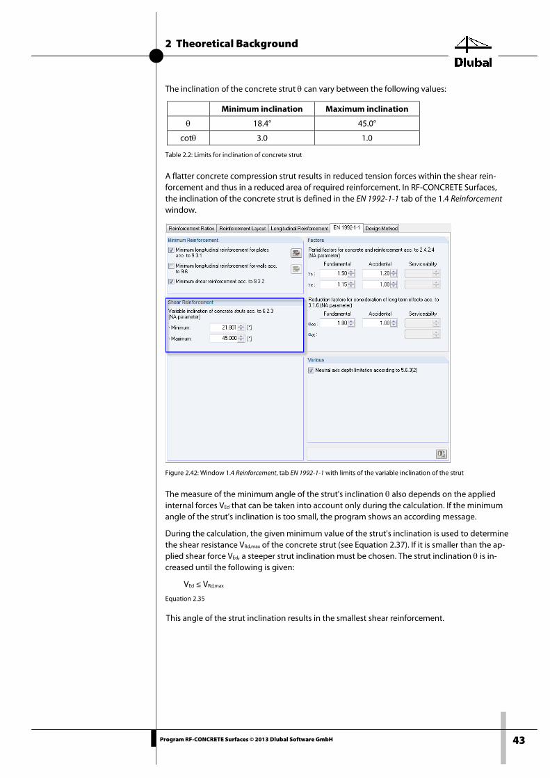
The inclination of the concrete strut θ can vary between the following values:
Minimum inclination Maximum inclination
θ 18.4° 45.0°
cotθ 3.0 1.0
Table 2.2: Limits for inclination of concrete strut
A flatter concrete compression strut results in reduced tension forces within the shear rein-forcement and thus in a reduced area of required reinforcement. In RF-CONCRETE Surfaces, the inclination of the concrete strut is defined in the EN 1992-1-1 tab of the 1.4 Reinforcement window.
Figure 2.42: Window 1.4 Reinforcement, tab EN 1992-1-1 with limits of the variable inclination of the strut
The measure of the minimum angle of the strut's inclination θ also depends on the applied internal forces VEd that can be taken into account only during the calculation. If the minimum angle of the strut's inclination is too small, the program shows an according message.
During the calculation, the given minimum value of the strut's inclination is used to determine the shear resistance VRd,max of the concrete strut (see Equation 2.37). If it is smaller than the ap-plied shear force VEd, a steeper strut inclination must be chosen. The strut inclination θ is in-creased until the following is given:
VEd ≤ VRd,max
Equation 2.35
This angle of the strut inclination results in the smallest shear reinforcement.

2 Theoretical Background
44 Program RF-CONCRETE Surfaces © 2013 Dlubal Software GmbH
2.4.4.3 Design of Concrete Strut
For structural components with shear reinforcement perpendicular to the component's axis (α = 90°), the shear resistance VRd is the smaller value from:
VRd,s = (Asw / s) · z · fywd · cot θ (6.8)
Equation 2.36
VRd,max = αcw · bw · z · ν1 · fcd / (cot θ + tan θ) (6.9)
Equation 2.37
where
Asw Cross-sectional area of shear reinforcement
s Spacing of links
fywd Design yield strength of the shear reinforcement
ν1 Reduction factor for concrete strength in case of shear cracks
αcw Coefficient taking account of the state of the stress in the compression chord
For structural components with an inclined shear reinforcement, the shear force resistance is the smaller value of:
VRd,s = (Asw / s) · z · fywd · (cot θ + cot α) · sin α (6.13)
Equation 2.38
VRd,max = αcw · bw · z · ν1 · fcd · (cot θ + cot α) / (1 + cot2θ) (6.14)
Equation 2.39
2.4.4.4 Example for Shear Design
We want to look at the shear design of a plate according to EN 1992-1-1 by means of the de-sign details (see the example for the statically required reinforcement, page 36).
In the details of the results, the shear forces determined in RFEM are shown at the beginning.
Figure 2.43: Internal forces of linear statics - shear forces

2 Theoretical Background
45 Program RF-CONCRETE Surfaces © 2013 Dlubal Software GmbH
The required longitudinal reinforcement is determined from these internal forces.
Figure 2.44: Required longitudinal reinforcement
The analysis of the shear resistance is shown in the details below. It starts with the determina-tion of the allowed tensile reinforcement in the direction of the principal shear force.
Figure 2.45:Shear Design - Applied tensile reinforcement
The second direction of reinforcement at the bottom surface of the plate and the first rein-forcement direction at the top surface of the plate are the only directions of reinforcement to which tension is assigned and which approximately run parallel to the direction of the princi-pal shear force.
These yield an Applied Longitudinal Reinforcement asl of 0.61 cm2/m.

2 Theoretical Background
46 Program RF-CONCRETE Surfaces © 2013 Dlubal Software GmbH
The design shear force VRd,c of the plate without shear reinforcement is determined with the following parameters:
CRd,c = 0.18 / γc = 0.18 / 1.15 = 0.12
k = 1 + √(200 / d) = 1 + √(200 / 160) = 2.11 ≤ 2.00 → k = 2.00 d in [mm]
d = 0.160 m
ρl = asl / (bw · d) = 0.613 / (100 · 16) = 0.000383 ≤ 0.02
bw = 1.00 m
fck = 20.0 N/mm2 for concrete C20/25
k1 = 0.15
σcp = 0.00 N/mm2
VRd,c = 0.12 · 2.00 · (100 · 0.000383 · 20)1/3 + 0.15 · 0.00 · 1000 · 160 = 35.135 kN/m
The same result can be found in the design details:
Figure 2.46: Shear design - shear resistance without shear reinforcement
The shear resistance VRd,c of the plate without shear reinforcement is compared to the applied shear force VEd.
VRd,c = 35.142 kN/m ≥ VEd = 29.56 kN/m
It has therefore been determined that the shear resistance of the plate without shear rein-forcement is sufficient and no further checks are necessary.
2.4.5 Reinforcement Rules For plates, the same reinforcement rules apply as presented in chapter 2.3.7, page 27.
In RF-CONCRETE Surfaces, user-defined specifications can be set in the 1.4 Reinforcement win-dow. The following tabs are relevant:
• Tab Reinforcement Layout (see Figure 3.26, page 149)
• Tab EN 1992-1-1 (see Figure 3.37, page 157)
If there are different specifications for the minimum shear reinforcement in the two tabs, the more unfavorable specification is applied.
2 Theoretical Background
47 Program RF-CONCRETE Surfaces © 2013 Dlubal Software GmbH
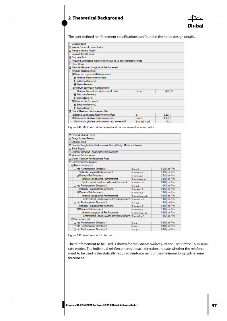
The user-defined reinforcement specifications can found in the in the design details.
Figure 2.47: Minimum reinforcement and maximum reinforcement ratio
Figure 2.48: Reinforcement to be used
The reinforcement to be used is shown for the Bottom surface (+z) and Top surface (-z) in sepa-rate entries. The individual reinforcements in each direction indicate whether the reinforce-ment to be used is the statically required reinforcement or the minimum longitudinal rein-forcement.

2 Theoretical Background
48 Program RF-CONCRETE Surfaces © 2013 Dlubal Software GmbH
2.5 Shells
2.5.1 Design Concept In terms of their internal forces, shells are a combination of walls (chapter 2.3) and plates (chapter 2.4), because they contain axial forces as well as moments.
All 3D model types (see Figure 2.1, page 10) are designed as shells. RF-CONCRETE Surfaces does this as follows: First, as shown in chapter 2.3 and 2.4, the design axial forces and design -bending moments are determined separately. Again, they are based on the principal axial forces and principal bending moments of the linear RFEM plate analysis.
Such a design axial force and design moment is determined for each direction of reinforce-ment on each surface side. One or both internal forces can become zero – if the search for the optimal direction of the concrete strut in the determination of the design internal forces re-sults in the fact that the reinforcement in this direction is not activated.
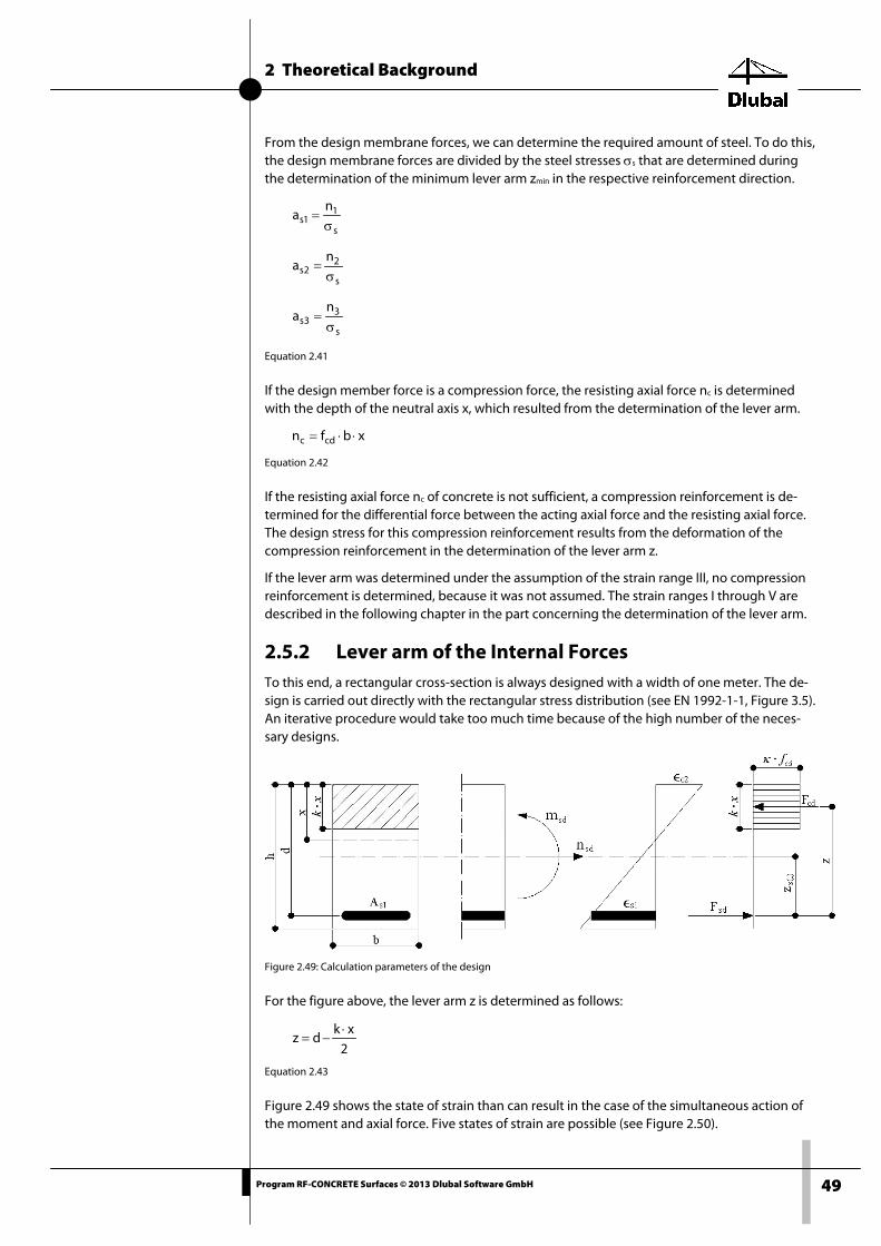
When the design internal forces are determined for the respective direction of reinforcement, the focus is on that direction of reinforcement for which design moments are available. For these moments, the program carries out a common one-dimensional design of a beam with the width of one meter. The goal of this design, however, is not to find a required reinforce-ment but to determine the lever arm of the internal forces.
When in this preliminary design the program has determined all lever arms of those design di-rections for which a design moment occurs, the program determines the smallest lever arm for each plate side. With this eccentricity, the moments of the linear plate analysis can now be transformed into membrane forces. To this end, the moments of the linear plate analysis is simply divided by the smallest lever arm zmin.
Now, if we add half the axial force from the linear plate analysis running perpendicular to the moment vector of the moment, which is divided by the lever arm of the internal forces, we ob-tain the final membrane force. This process can be expressed as follows:
2
n
z
mn x
min
xxs +=
2
n
z
mn y
min
yys +=
2
n
z
mn xy
min
xyxys +=
Equation 2.40
The moments at the top and bottom surface of the plate are considered with different signs.
The moments mx, my, and mxy and the axial forces nx, ny, and nxy of the linear plate analysis are substituted by means of the lever arm zmin from the preliminary design by the membrane forc-es nxs, nys, and nxys. When this is done, the principal membrane forces nIs and nIIs can be deter-mined from these membrane forces for the bottom and top surface of the plate.
From the principal membrane forces nIs and nIIs, the design membrane forces (see chapter 2.3, page 14) nα, nβ, and nγ are determined according to Equation 2.5 through Equation 2.7. The design membrane forces nα, nβ, and nγ are then assigned to the reinforcement directions ϕ1, ϕ2, and ϕ3. We obtain the design membrane forces n1, n2, and n3 in the reinforcement directions.
2 Theoretical Background
49 Program RF-CONCRETE Surfaces © 2013 Dlubal Software GmbH
From the design membrane forces, we can determine the required amount of steel. To do this, the design membrane forces are divided by the steel stresses σs that are determined during the determination of the minimum lever arm zmin in the respective reinforcement direction.
s
11s
na
σ=
s
22s
na
σ=
s
33s
na
σ=
Equation 2.41
If the design member force is a compression force, the resisting axial force nc is determined with the depth of the neutral axis x, which resulted from the determination of the lever arm.
xbfn cdc ⋅⋅=
Equation 2.42
If the resisting axial force nc of concrete is not sufficient, a compression reinforcement is de-termined for the differential force between the acting axial force and the resisting axial force. The design stress for this compression reinforcement results from the deformation of the compression reinforcement in the determination of the lever arm z.
If the lever arm was determined under the assumption of the strain range III, no compression reinforcement is determined, because it was not assumed. The strain ranges I through V are described in the following chapter in the part concerning the determination of the lever arm.
2.5.2 Lever arm of the Internal Forces To this end, a rectangular cross-section is always designed with a width of one meter. The de-sign is carried out directly with the rectangular stress distribution (see EN 1992-1-1, Figure 3.5). An iterative procedure would take too much time because of the high number of the neces-sary designs.
Figure 2.49: Calculation parameters of the design
For the figure above, the lever arm z is determined as follows:
2xk
dz⋅
−=
Equation 2.43
Figure 2.49 shows the state of strain than can result in the case of the simultaneous action of the moment and axial force. Five states of strain are possible (see Figure 2.50).

2 Theoretical Background
50 Program RF-CONCRETE Surfaces © 2013 Dlubal Software GmbH
Figure 2.50: Areas of strain distribution
Range I
This shows a cross-section subjected to great bending. The depth of the neutral axis has reached its maximum value (x = ξlim ⋅ d). Another increase of the section modulus is now only possible by using a compression reinforcement.
Range II
Mainly compression occurs in this range. The depth of the neutral axis is between the limits ξlim ⋅ d and h/k.
Range III
The applied moment is so small that the concrete compression zone (neutral axis) without the compression reinforcement can result in a sufficient section modulus. Depending on the ap-plied moment, the limits of the neutral axis are between 0 and ξlim ⋅ d.
Range IV
This range shows a fully compressed cross-section. The depth of the neutral axis is greater than h/k. This area also includes cross-sections that are subjected to compression only.
Range V
This state of strain is present if the tension force cracks a cross-section completely. This range also includes cross-sections that are subject to tension forces only.
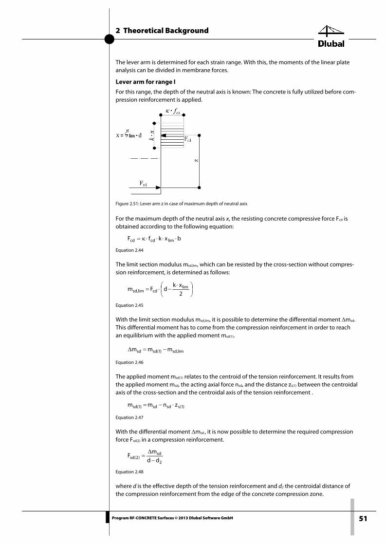
2 Theoretical Background
51 Program RF-CONCRETE Surfaces © 2013 Dlubal Software GmbH
The lever arm is determined for each strain range. With this, the moments of the linear plate analysis can be divided in membrane forces.
Lever arm for range I
For this range, the depth of the neutral axis is known: The concrete is fully utilized before com-pression reinforcement is applied.
Figure 2.51: Lever arm z in case of maximum depth of neutral axis
For the maximum depth of the neutral axis x, the resisting concrete compressive force Fcd is obtained according to the following equation:
bxkfF limcdcd ⋅⋅⋅⋅κ=
Equation 2.44
The limit section modulus msd,lim, which can be resisted by the cross-section without compres-sion reinforcement, is determined as follows:
⋅
−⋅=2
xkdFm lim
cdlim,sd
Equation 2.45
With the limit section modulus msd,lim, it is possible to determine the differential moment ∆msd. This differential moment has to come from the compression reinforcement in order to reach an equilibrium with the applied moment msd(1).
lim,sd)1(sdsd mmm −=∆
Equation 2.46
The applied moment msd(1) relates to the centroid of the tension reinforcement. It results from the applied moment msd, the acting axial force nsd, and the distance zs(1) between the centroidal axis of the cross-section and the centroidal axis of the tension reinforcement .
)1(ssdsd)1(sd znmm ⋅−=
Equation 2.47
With the differential moment ∆msd , it is now possible to determine the required compression force Fsd(2) in a compression reinforcement.
2
sd)2(sd dd
mF
−∆
=
Equation 2.48
where d is the effective depth of the tension reinforcement and d2 the centroidal distance of the compression reinforcement from the edge of the concrete compression zone.

2 Theoretical Background
52 Program RF-CONCRETE Surfaces © 2013 Dlubal Software GmbH
If we divide the applied moment msd(1) that is related to the centroid of the tension reinforce-ment by the compression force Fcd and the force in the compression reinforcement Fsd(2), we obtain the lever arm z.
)2(sdcd
sd
FF
mz
+=
Equation 2.49
Lever arm for range II
Figure 2.52: Determination of the lever arm for range II
In order to be able to determine the depth of the concrete neutral axis x, we first determine the design moment msd(2) about the centroid of the compression reinforcement.
)2(ssdsd)2(sd znmm ⋅+=
Equation 2.50
Now the sum of the moments about the centroid of the compression reinforcement is calcu-lated. These moments must result as equal to zero. On the side of the resistance, the moment is calculated from the resulting force Fcd of the concrete compression zones times its distance. In range II, there is no reinforcement in tension.
0md2
xkFm )2(sd2cd =+
−
⋅⋅=∑
Equation 2.51
The resulting concrete compression force Fcd also contains the depth x of the concrete neutral axis.
bxkfF cdcd ⋅⋅⋅⋅κ=
Equation 2.52
Thus, the equation for the determination of x is obtained as:
0mdbxkf2
xkbfmd
2
xkbxkf )2(sd2cd
22cd
)2(sd2cd =+⋅⋅⋅⋅⋅κ−⋅⋅⋅⋅κ
=+
−
⋅⋅⋅⋅⋅⋅κ
0kbf
m2
k
xd2x
2cd
)2(sd22 =⋅⋅⋅κ
⋅+
⋅⋅− ⇒ 2
cd
)2(sd2
22
kbf
m2
k
d
k
dx
⋅⋅⋅κ
⋅−
+=
Equation 2.53

2 Theoretical Background
53 Program RF-CONCRETE Surfaces © 2013 Dlubal Software GmbH
With the depth x of the neutral axis, it is possible to determine the lever arm z by subtracting from the effective height d half the depth of the neutral axis x, which is reduced by the factor x:
2xk
dz⋅
−=
Equation 2.54
Lever arm for range III
Figure 2.53: Determination of the lever arm for range III
To determine the depth x of the neutral axis, we first determine the design moment msd(1) about the centroid of the tension reinforcement.
)1(ssdsd)1(sd znmm ⋅−=
Equation 2.55
Now the sum of the moments about the centroid of the tension reinforcement is calculated. These moments must result as equal to zero. On the resistance side, the moment is calculated only from the resulting force Fcd of the concrete neutral axis times its distance. Then, the equi-librium of the moments about the position of the tension reinforcement is calculated.
0m2
xkdFm )1(sdcd =−
⋅
−⋅=∑
Equation 2.56
The depth x of the concrete neutral axis is also contained in the resulting concrete compression force Fcd (see Equation 2.52).
0bkf
m2x
k
d2xmx
2
bkfxdbkf
2cd
)1(sd2)1(sd
22
cdcd =
⋅⋅⋅κ
⋅+⋅
⋅−=−⋅
⋅⋅⋅κ−⋅⋅⋅⋅⋅κ
Equation 2.57
This quadratic equation can be solved as follows.
bkf
m2
k
d
k
dx
2cd
)1(sd2
2
⋅⋅⋅κ
⋅−+=
Equation 2.58
With the depth x of the concrete neutral axis, the lever arm z can be determined by subtracting from the effective height d half the depth of the neutral axis x, which is multiplied by factor k:
2xk
dz⋅
−=
Equation 2.59
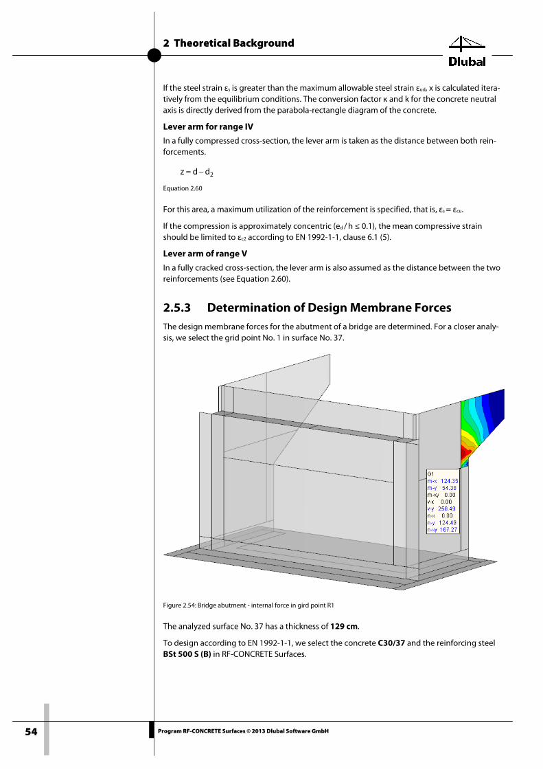
2 Theoretical Background
54 Program RF-CONCRETE Surfaces © 2013 Dlubal Software GmbH
If the steel strain εs is greater than the maximum allowable steel strain εud, x is calculated itera-tively from the equilibrium conditions. The conversion factor κ and k for the concrete neutral axis is directly derived from the parabola-rectangle diagram of the concrete.
Lever arm for range IV
In a fully compressed cross-section, the lever arm is taken as the distance between both rein-forcements.
2ddz −=
Equation 2.60
For this area, a maximum utilization of the reinforcement is specified, that is, εs = εcu.
If the compression is approximately concentric (ed / h ≤ 0.1), the mean compressive strain should be limited to εc2 according to EN 1992-1-1, clause 6.1 (5).
Lever arm of range V
In a fully cracked cross-section, the lever arm is also assumed as the distance between the two reinforcements (see Equation 2.60).
2.5.3 Determination of Design Membrane Forces The design membrane forces for the abutment of a bridge are determined. For a closer analy-sis, we select the grid point No. 1 in surface No. 37.
Figure 2.54: Bridge abutment - internal force in gird point R1
The analyzed surface No. 37 has a thickness of 129 cm.
To design according to EN 1992-1-1, we select the concrete C30/37 and the reinforcing steel BSt 500 S (B) in RF-CONCRETE Surfaces.
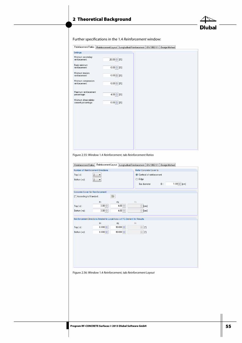
2 Theoretical Background
55 Program RF-CONCRETE Surfaces © 2013 Dlubal Software GmbH
Further specifications in the 1.4 Reinforcement window:
Figure 2.55: Window 1.4 Reinforcement, tab Reinforcement Ratios
Figure 2.56: Window 1.4 Reinforcement, tab Reinforcement Layout

2 Theoretical Background
56 Program RF-CONCRETE Surfaces © 2013 Dlubal Software GmbH
Figure 2.57: Window 1.4 Reinforcement, tab Longitudinal Reinforcement
Figure 2.58: Window 1.4 Reinforcement, tab EN 1992-1-1
Figure 2.59: Window 1.4 Reinforcement, tab Design Method

2 Theoretical Background
57 Program RF-CONCRETE Surfaces © 2013 Dlubal Software GmbH
2.5.3.1 Design Moments
The design details of the grid points show the internal forces interpolated from the FE nodes. In the General Data, the 3D type of model was specified (see Figure 2.1, page 10). Hence, there are the moments mx, my, and mxy as well as the axial forces nx, ny, and nxy in the surface.
Figure 2.60: Internal forces of linear analysis
The principal internal forces are determined from the RFEM internal forces of the linear analy-sis. The principal internal forces are determined according to the equations described in the chapters 2.3 and 2.4.
Figure 2.61: Principal internal forces
For shells, the principal axial forces are shown for both plate surfaces, because they are re-quired for the shell design. Unlike the moments, the principal axial forces at the bottom and top surface of the plate are the same.
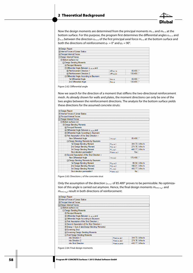
2 Theoretical Background
58 Program RF-CONCRETE Surfaces © 2013 Dlubal Software GmbH
Now the design moments are determined from the principal moments mI,+z and mII,+z at the bottom surface. For this purpose, the program first determines the differential angles αm,+z and βm,+z between the direction αm,+z of the first principal axial force mI,+z at the bottom surface and both the directions of reinforcement ϕ1 = 0° and ϕ2 = 90°.
Figure 2.62: Differential angle
Now we search for the direction of a moment that stiffens the two-directional reinforcement mesh. As already shown for walls and plates, the moment directions can only be one of the two angles between the reinforcement directions. The analysis for the bottom surface yields these directions for the assumed concrete struts:
Figure 2.63: Directions γ of the concrete strut
Only the assumption of the direction γm,+z,1 of 85.489° proves to be permissible. No optimiza-tion of this angle is carried out anymore. Hence, the final design moments mend,+z,ϕ1 and mend,+z,ϕ2 result in both directions of reinforcement:
Figure 2.64: Final design moments

2 Theoretical Background
59 Program RF-CONCRETE Surfaces © 2013 Dlubal Software GmbH
2.5.3.2 Design Axial Forces The design axial forces nend,+z,ϕ1, and nend,+z,ϕ2 are determined according to the same principle.
Figure 2.65: Design axial forces
2.5.3.3 Lever of Internal Forces With the design internal forces for the directions of reinforcement ϕ1 = 0° and ϕ2 = 90°, it is now possible to determine the lever arm of the internal forces.
Figure 2.66: Design internal forces
As described in chapter 2.5.2 on page 49, a preliminary design is carried out with both deter-mined internal forces for both directions of reinforcement. This preliminary design serves to determine the lever arm of the internal forces. The lever arm is determined from the state of strain due to the design internal forces (see the following figure).

2 Theoretical Background
60 Program RF-CONCRETE Surfaces © 2013 Dlubal Software GmbH
Figure 2.67: Lever arm of internal forces
The value 1.239 m is obtained for the smaller and, therefore, governing lever arm zmin,+z.
2.5.3.4 Membrane Forces With the governing lever arm from the preliminary design, it is now possible to transform the internal forces of the linear plate analysis into membrane forces. To this end, the equations presented on page 48 are used.
m/kN408.482
911.103
239.1
35.124
2
n
z
mn x
zmin,
xz,sx =
−+=+=
++
m/kN819.982
386.285239.1
36.542
n
z
mn y
zmin,
yz,sy −=
−+=+=
++
m/kN910.1092935.135
239.139.220
2
n
z
mn xy
zmin,
xyz,xy −=+
−=+=
++
These membrane forces can also be found in the design details.
Figure 2.68: Membrane forces
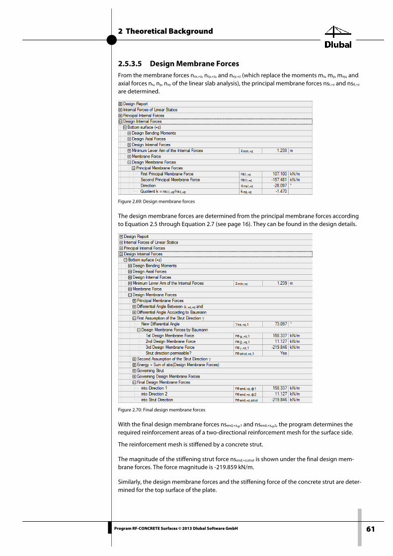
2 Theoretical Background
61 Program RF-CONCRETE Surfaces © 2013 Dlubal Software GmbH
2.5.3.5 Design Membrane Forces From the membrane forces nsx,+z, nsy,+z, and nxy,+z (which replace the moments mx, my, mxy, and axial forces nx, ny, nxy of the linear slab analysis), the principal membrane forces nsI,+z and nsII,+z are determined.
Figure 2.69: Design membrane forces
The design membrane forces are determined from the principal membrane forces according to Equation 2.5 through Equation 2.7 (see page 16). They can be found in the design details.
Figure 2.70: Final design membrane forces
With the final design membrane forces nsend,+z,ϕ1 and nsend,+z,ϕ2, the program determines the required reinforcement areas of a two-directional reinforcement mesh for the surface side.
The reinforcement mesh is stiffened by a concrete strut.
The magnitude of the stiffening strut force nsend,+z,strut is shown under the final design mem-brane forces. The force magnitude is -219.859 kN/m.
Similarly, the design membrane forces and the stiffening force of the concrete strut are deter-mined for the top surface of the plate.

2 Theoretical Background
62 Program RF-CONCRETE Surfaces © 2013 Dlubal Software GmbH
2.5.4 Analysis of Concrete Struts To analyze the concrete strut of a shell, it is divided in three surface layers that are subjected to the design membrane forces.
Figure 2.71: Surface layers thicknesses for shells mainly subjected to moments (left) and compression force (right)
For shells, where the applied moment is relatively great in relation to the applied axial force (ed h > 0.2), the thickness hE of the two outer layers is reduced to 0.35 · d. For shells subjected to approximately concentric compression, the equivalent layer thickness hE is increased to half the plate thickness h. If the relative eccentricity of the axial force ed / h is between 0 and 0.2, then the thickness of the layers is interpolated.
For ed, the greater value of the quotients of mx /nx and my / ny is taken.
For the analysis of the concrete strut, the strut's compression force to be resisted, nstrut,+z, is compared to the resisting axial force of the equivalent layer nstrut,d.
Figure 2.72: Concrete strut and thickness of equivalent layer
The resisting axial force nstrut,d depends on the thickness hE of the equivalent layer and the ap-plied concrete strength fcd,08.
The first step to determine the thickness of the equivalent layer is to determine the provided load eccentricities in x- and y-direction from the internal forces of the linear plate analysis:
m197.1911.10335.124
n
me
x
xdx =
−==
m190.0386.285
36.54n
me
y
ydy =
−==

2 Theoretical Background
63 Program RF-CONCRETE Surfaces © 2013 Dlubal Software GmbH
The greatest load eccentricity in x-direction is computed as governing. This can be used to de-termine the relative load eccentricity ed / h.
2.0928.029.1
197.1h/ed >==
Since the relative load eccentricity is greater than 0.2, this is regarded as a shell that is predom-inantly subjected to bending. The factor fhE for the determination of the equivalent layer thick-ness is 0.35.
The thickness hE of the equivalent layer is therefore determined as follows:
hE = fhE · h = 0.35 · 129 = 45.15 cm
The design value of the concrete compressive strength is reduced according to the recom-mendations from SCHLAICH/SCHÄFER (in: Betonkalender 1993/II, page 378) to 80 %. This recom-mendation can also be found in EN 1992-1-1, clause 6.5.2, regulating the design of struts in strut-and-tie models.
fcd = fck / γc = 30 / 1.5 = 20 N/mm2
fcd,08 = 0.8 · 20 = 16 N/mm2
This value can also be found in the design details (see Figure 2.72).
With this value, it is possible to determine the resisting force of the concrete strut nstrut,d.
nstrut,d = b · hE · fcd,08 = 100 · 45.15 · 16 = 7224.00 kN/m
The analysis of the concrete strut for the top surface is done similarly.
2.5.5 Required Longitudinal Reinforcement The longitudinal reinforcement to be used at the bottom surface is determined from the de-sign membrane forces. In the design details, the output is subdivided for the two directions of reinforcement.
Figure 2.73: Required longitudinal reinforcement
m/cm40.393.465
344.158nsa 2
1,z,s
1,z,end1,zdim,s ==
σ=
+
ϕ++
m/cm24.093.465
116.11nsa 2
2,z,s
2,z,end2,zdim,s ==
σ=
+
ϕ++
The reinforcement for the top surface is determined similarly.

2 Theoretical Background
64 Program RF-CONCRETE Surfaces © 2013 Dlubal Software GmbH
2.5.6 Shear Design In the shear design, the applied tension reinforcement is determined first.
Figure 2.74: Applied tension reinforcement
From all reinforcement layers and directions, a total of 1.54 2/m tension reinforcement can be applied. With this, the resisting shear force VRd,c without shear reinforcement is determined.
Figure 2.75: Design shear resistance without shear reinforcement

2 Theoretical Background
65 Program RF-CONCRETE Surfaces © 2013 Dlubal Software GmbH
With the applied longitudinal reinforcement ratio, the longitudinal reinforcement ratio ρl is determined:
ρl = Asl / (bw · d) = 1.54 / (100 · 125.5) = 0.00012 ≤ 0.02
In a 3D type of model (unlike in a plate), an additional axial force can occur. It must be consid-ered by using the according concrete longitudinal stress.
σcp = Nβ / (bw · h) = -425.783 / (100 · 129) = - 0.33 N/m2
The factor for taking account of the plate depth is calculated as follows:
k = 1 + √(200 / d) = 1 + √(200 / 1255) = 1.399 ≤ 2.0 d in mm
Moreover, the following factors are included in the design:
Factor of concrete longitudinal stress k1 = 0.15
Concrete compressive strength for C30/37 fck = 30.0 N/mm2
Safety factor Crd,c = 0.18 / γc = 0.18 / 1.5 = 0.12
Thus, the design shear resistance VRd,c without shear reinforcement can be determined accord-ing to Equation (6.2a):
VRd,c = Crd,c · k · (100 · ρl · fck)1/3 + k1 · σcp · bw · d =
= 0.12 · 1.399 · (100 · 0.00012 · 30.0)1/3 + 0.15 · 0.33 · 1000 · 1255 = 212.00 kN/m
The minimum value of the design shear resistance VRd,c without shear reinforcement is deter-mined according to Equation (6.2b) from the minimum reinforcement ratio νmin:
νmin = 0.035 · k3/2 · fck1/2 = 0.035 · 1.3993/2 · 30.01/2 = 0.317
VRd,c = (0.317 + 0.15 · 0.33) · 1000 · 1255 = 459.96 kN/m
The design shear resistance of the plate, VRd,c = 459.96 kN/m, is greater than the applied shear force VEd = 259.726 kN/m. Hence, no shear reinforcement is required in the example.
If the shear resistance of the plate is not sufficient, the program first checks if the maximum shear resistance of the concrete strut VRd,max is sufficient. VRd,max is determined with the mini-mum inclination of the strut θ. If the design shear resistance of the concrete strut is greater than the applied shear force VEd, it is possible to determine the statically required shear rein-forcement req asw. Then, the design for the shear reinforcement VRd,sy is carried out.

2 Theoretical Background
66 Program RF-CONCRETE Surfaces © 2013 Dlubal Software GmbH
2.5.7 Statically Required Longitudinal Reinforcement The table of the design details summarizes the statically required longitudinal reinforcement.
Figure 2.76: Statically required longitudinal reinforcement
For each direction of reinforcement, the table shows which design is governing for the statical-ly required reinforcement.
In the example, all longitudinal reinforcements result from the bending design as shell. In oth-er cases, a required longitudinal reinforcement to avoid shear reinforcement would also be possible.
2.5.8 Minimum Longitudinal Reinforcement The statically required longitudinal reinforcement is now compared to the minimum rein-forcement. Unfortunately, none of the standards available in RF-CONCRETE Surfaces provide any regulations on the minimum reinforcement for shells. Therefore, we have to analyze in which constellation of moment and axial force we regard the element as a wall (mainly sub-jected to compression) or a plate (mainly subjected to bending). The distinguishing criterion is the related load eccentricity ed / h in the ultimate limit state (ULS):
hnm
h
ed =
Equation 2.61
where
m Moment of linear plate analysis (ULS)
n Axial force of linear plate analysis (ULS)
h Plate depth
In a design point, there are moments and axial forces in x- as well as y-direction. Hence, the relative load eccentricity for each design point is the greatest quotient from moment over axial force of both directions.
In RF-CONCRETE Surfaces, the following is equally specified for all standards:
:5.3h
ed > Mainly subjected to bending ⇒ reinforcement rules for plates
:5.3h
ed ≤ Mainly subjected to compression ⇒ reinforcement rules for walls
This rule can be found in EN 1992-1-1, clause 9.3: Solid slabs, and clause 9.6: Walls. The mini-mum reinforcements are described in chapter 2.3.7, page 25, and chapter 2.4.5, page 46 in the reinforcement rules for walls and plates.
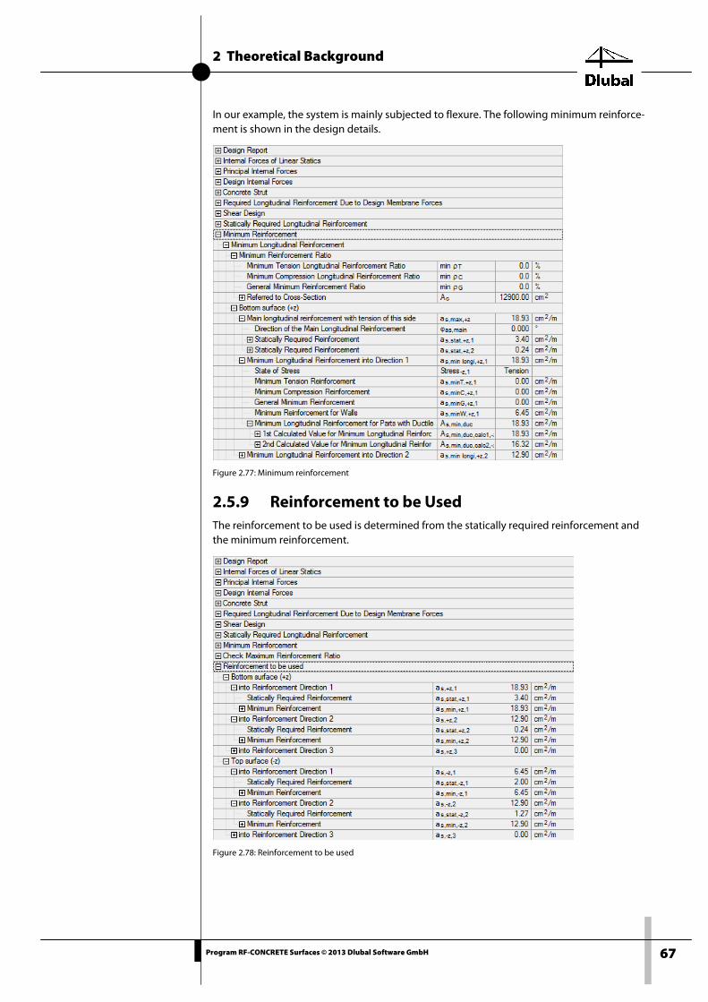
2 Theoretical Background
67 Program RF-CONCRETE Surfaces © 2013 Dlubal Software GmbH
In our example, the system is mainly subjected to flexure. The following minimum reinforce-ment is shown in the design details.
Figure 2.77: Minimum reinforcement
2.5.9 Reinforcement to be Used The reinforcement to be used is determined from the statically required reinforcement and the minimum reinforcement.
Figure 2.78: Reinforcement to be used
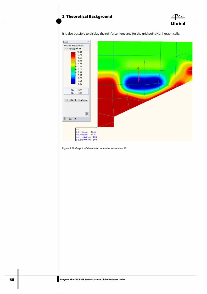
2 Theoretical Background
68 Program RF-CONCRETE Surfaces © 2013 Dlubal Software GmbH
It is also possible to display the reinforcement area for the grid point No. 1 graphically.
Figure 2.79: Graphic of the reinforcement for surface No. 37
2 Theoretical Background
69 Program RF-CONCRETE Surfaces © 2013 Dlubal Software GmbH
2.6 Serviceability Limit State The serviceability limit state designs consist of various individual designs that are specified in the following Eurocode chapters. The relevant clauses for EN 1992-1-1 are:
• Limitation of stresses: clause 7.2
• Crack control: clause 7.3
• Deflection control: clause 7.4
In the reinforced concrete standards, the designs listed above are always described for linear elements. In the ultimate limit state, as mentioned in the previous part of this manual, the de-sign situation of a surface element is transformed into the design of several linear elements in the individual reinforcement directions. The transformation procedure is also used in the ser-viceability limit state.
2.6.1 Design Internal Forces Unlike the transformation procedure for the ultimate limit state, it is not possible to carry out a purely geometrical division of the principal internal forces into forces in the individual direc-tions of reinforcement. Such a division assumes a deformation ratio of 1.0 for the actual provid-ed reinforcement. To have the same strain in both reinforcement directions for different design forces in these directions of reinforcement, however, according reinforcement areas would have to be provided. In the serviceability limit state, however, the design internal forces are searched for a provided reinforcement.
In the serviceability limit state, no required reinforcement is determined. Instead, the actual provided deformation ratio is determined with the provided reinforcement. In all cases in which the applied reinforcement deviates from the required reinforcement, the actual provid-ed deformation ratio of the reinforcements does not equal the value 1.0.
Thus, the assumption of an identical deformation ratio is therefore not valid. A different de-formation ratio must be found that confirms its resulting design internal forces. In solving this problem, the geometrical relationship between the deformation ratio and the direction of the concrete strut plays an important role.
BAUMANN [1] writes the following on this point: If we neglect the compression strain of the con-crete because it usually small compared to the strain of the reinforcement, we obtain from Figure 38 the compatibility condition
( )α−γ−
=ε
ε2
2
x
y
sin
)yß(sin
Equation 2.62
The figure on the following page represents the "Figure 38" mentioned by Baumann. It repre-sents the compatibility condition of the strains in a two-directional reinforcement mesh.

2 Theoretical Background
70 Program RF-CONCRETE Surfaces © 2013 Dlubal Software GmbH
Figure 2.80: Compatibility of the strains
In Equation 2.62, εy and εx are the strains of two reinforcement directions. The angles α and β represent the intermediate angles between the principal force direction and the respective di-rection of reinforcement. The smaller intermediate angle is called α. The angle γ refers to the differential angle between the direction of the concrete strut and the direction of the first principal internal force.
The angles α and β cannot be changed by selecting the reinforcement direction. In contrast to this, the angle γ changes if due to the differently stiff directions of reinforcement a different di-rection of the concrete strut is necessary to stiffen the reinforcement mesh.
The design internal forces in the individual directions of reinforcement depend on the selected direction of the concrete strut. With these design internal forces, it is possible to determine the stresses in the reinforcements of the individual directions. Based on these stresses, the various standards give equations with which it is possible to determine the mean strains of the rein-forcement relative to the concrete. In EN-1992-1-1, this is done according to Equation (7.9):
( )
s
s
s
eff,peeff,p
eff,ctts
cmsm E6.0
E
1f
kσ
⋅≥
ρ⋅α+⋅ρ
⋅−σ
=ε−ε
Equation 2.63
Then, it is possible to determine the quotient from the differences of the strains between con-crete and reinforcing steel of the second and first reinforcement direction.
1cmsm
2cmsm
)(
)(Q
ϕ
ϕε ε−ε
ε−ε=
Equation 2.64
Equation 2.62 also gives a quotient of the strains, derived from the geometric relationships.
( )α−γ−
=ε
ε=
ϕ
ϕε 2
2
1
2geo,
sin
)yß(sinQ
Equation 2.65

2 Theoretical Background
71 Program RF-CONCRETE Surfaces © 2013 Dlubal Software GmbH
For both quotients, the strain of the second direction of reinforcement is in the numerator. This is based on the assumption that the first reinforcement direction forms the smaller differ-ential angle with the first principal internal force. If the second reinforcement direction with the first principal internal force forms the smaller differential angle, the strain of the first rein-forcement direction would be in the numerator of the quotient.
Both quotients depend on the selected direction of the concrete strut. Now the program tries to select the direction of the concrete strut in such a way that both quotients become identi-cal.
geo,QQ εε =
Equation 2.62
If after one calculation run the geometrical deformation ratio Qε,geo still does not correspond to the actual deformation ratio, the program specifies a new direction of the concrete strut and determines its resulting geometric deformation ratio. This process is repeated iteratively until a convergence is reached.
The determination of the design internal forces by means of the selection of the appropriate concrete strut direction is the most demanding part of the serviceability limit state design. If the selected provided reinforcement approximately corresponds to the statically required rein-forcement for the analyzed service load magnitudes, the design internal forces only marginally differ from those internal forces that would result from an assumed strain ratio of 1.0. There-fore, RF-CONCRETE Surfaces offers the possibility to determine the design internal forces with an assumed deformation ratio of 1.0
The design internal forces for the serviceability limit state design are determined only if the cracking of the concrete leads to an activation of the reinforcement. To this end, the program analyzes the concrete tensile stresses caused by the first principal internal force.
2.6.2 Principal Internal Forces If the first principal internal force is negative, we assume uncracked concrete in the area of the analyzed surface element. For walls, only the magnitude of the concrete stress is checked. For plates, at least at this surface side no serviceability limit state design is carried out.
If for a Wall, the first principal axial force is a tension force, the provided concrete tensile stress is determined according to the following equation.
hb
n
A
n I
c
II,c ⋅
==σ
Equation 2.62
If for a Plate the first principal moment is a positive moment, the provided concrete tensile stress is determined as follows.
2II
I,chb
6m
W
m
⋅⋅
==σ
Equation 2.62
If the linear-elastically determined stress σc,I is greater than the mean axial tensile strength fctm, a cracked concrete is assumed. Only then does RF-CONCRETE Surfaces determine the design internal forces for the individual directions of reinforcement and performs the serviceability limit state designs mentioned at the beginning of chapter 2.6.

2 Theoretical Background
72 Program RF-CONCRETE Surfaces © 2013 Dlubal Software GmbH
2.6.3 Provided Reinforcement Before RF-CONCRETE Surfaces designs the serviceability limit state, it checks the provided rein-forcement: First, the program uses the internal forces of the serviceability to perform a design like for the ultimate limit state. The design results in a structurally required reinforcement which is then compared to the user-defined provided reinforcement.
If the provided reinforcement is smaller than the statically required reinforcement, or if the de-sign reveals any non-designable situations, the serviceability limit state design will not be per-formed. The problematic zones of the surface elements are indicated as non-designable.
2.6.4 Serviceability Limit State Designs The following example illustrates how the various serviceability limit state designs are imple-mented in RF-CONCRETE Surfaces. In this example, we analyze a rectangular slab. The first ap-plied principal moment mI is greater than zero, the second applied moment mII equals zero.
The design is carried out according to EN 1992-1-1 according to the analytical method.
2.6.4.1 Input Data for Example
Geometric specifications
Slab depth: d = 20 cm
Rectangular reinforcement: ф1 = 30° ф2 = 120°
Centroid of concrete cover: d1 = 3.0 cm d2 = 4.2 cm
Material
Concrete: C30/37
Reinforcing steel: B 500 S (B)
2.6.4.2 Check of Principal Internal Forces First, the program checks if the concrete cracks under the principal moment at the ULS. In the serviceability design details of the relevant grid point, you can see that this is indeed the case:
Figure 2.81: Checking the principal internal forces
The linear-elastically determined stress σc,I,-z at the upper concrete edge is compared to the mean axial tensile strength fctm of 2.9 N/mm2 for a concrete C30/37.
222
z,Iz,I,c mm/N05.5
2.00.1
665.33
hb
6mW
m=
⋅⋅
=⋅⋅
==σ −−
The concrete edge strain σc,I,-z = 5.05 N/mm2 thus clearly exceeds the tensile strength fctm. Therefore, the reinforcement is activated for the serviceability limit state, too.

2 Theoretical Background
73 Program RF-CONCRETE Surfaces © 2013 Dlubal Software GmbH
2.6.4.3 Required Reinforcement for ULS
The ultimate limit state design for the top surface of the plate is carried out with the following values:
Figure 2.82: Design internal forces ULS
Final design bending moments: mend,-z,ф1 = 64.16 kNm/m
mend,-z,ф2 = 42.08 kNm/m
mend,-z,strut = -38.23 kNm/m
Direction of concrete strut: фstrut,m,-z = 75.0°
From the design internal forces, we obtain the following required reinforcement for the top surface:
Figure 2.83: Required reinforcement

2 Theoretical Background
74 Program RF-CONCRETE Surfaces © 2013 Dlubal Software GmbH
2.6.4.4 Specification of a Reinforcement
At the top surface of the plate, we select for both directions a reinforcement from the rebars with the diameter ds of 12 mm at a distance ls of 10.0 cm.
The following provided reinforcement results:
( )m/cm31.11
cm0.10
m/cm100
4
cm2.1
l
m/cm100
4
daprov 2
2
s
2s
z,1s =⋅π⋅=⋅π⋅=−
We enter these values in the Longitudinal Reinforcement tab of the 1.4 Reinforcement window. Alternatively, they can be selected by means of the [Rebars] button (see Figure 2.105, page 86).
Figure 2.84: Window 1.4 Reinforcement, tab Longitudinal Reinforcement to define basic and additional reinforcement
With this reinforcement diameter, we obtain the following centroids of the concrete cover:
Figure 2.85: Window 1.4 Reinforcement, tab Reinforcement Layout
The effective depth for the individual directions of reinforcement is determined as follows:
d1,-z = h – d1 = 20 – 3 = 17 cm
d2,-z = h – d2 = 20 – 4.2 = 15.8 cm

2 Theoretical Background
75 Program RF-CONCRETE Surfaces © 2013 Dlubal Software GmbH
2.6.4.5 Check of the Provided Reinforcement for SLS
First, the deformation ratio εф2 / εф1 = 1.0 is assumed for the serviceability limit state. Thus, the following values are determined:
Figure 2.86: Design moments in SLS for deformation ratio of 1.0
Design internal forces: mend,-z,ф1 = 38.49 kNm/m
mend,-z,ф2 = 25.25 kNm/M
Stiffening compression moment: mend,-z,strut = -22.94 kNm/
Direction of stiffening compression moment фstrut,m,-z = 75.0°
For these design moments, the program determines at the top surface of the plate a required reinforcement of as,dim,-z,1 = 4.54 cm2/m in the first direction of reinforcement. The required rein-forcement in the second direction is as,dim,-z,1 = 3.17 cm2/m.
Figure 2.87: Statically required reinforcement for internal forces in SLS
The required reinforcement for the internal forces of the serviceability limit state is smaller than the user-defined provided reinforcement. Thus, it is possible to continue with the analy-sis.

2 Theoretical Background
76 Program RF-CONCRETE Surfaces © 2013 Dlubal Software GmbH
2.6.4.6 Selection of the Concrete Strut
With the design internal forces mend,-z,ф1 = 38.9 kNm/m and mend,-z,ф2 = 25.25 kNm/m, we obtain the strains εф1 = 0.735 ‰ in the first direction of reinforcement and εф2 = 0.527 ‰ in the sec-ond direction of reinforcement. Thus, the deformation ratio Qs,-z is 0.717.
Therefore, the assumed deformation ratio of 1.00 does not correspond to the actual deforma-tion ratio. The inclination of the stiffening compression moment is therefore increased from 75.0° to 79.746°.
Geometrically, this inclination of the stiffening compression moment can appear only if the geometrical relation Qs,,geo,-z of the strain in the reinforcement direction ф2 to the strain in the direction of the ф1 is ca. 0.717. This is indeed the case in our example.
When determining the crack width wk, it is shown that with the design moments for an inclina-tion of the stiffening compression moment of 79.746°, strains result in the individual directions of reinforcement that lead to the deformation ratio Qs,,geo,-z of 0.717.
Figure 2.88: Direction of the concrete strut and deformation ratios
The selected inclination of the stiffening compression moment of 79.746° results in modified design moments in the individual directions of reinforcement. This corresponds to the method for the determination of the design internal forces in in SLS taking into account the deforma-tion ratio of the longitudinal reinforcement that was selected in the dialog box Settings for Analytical Method of Serviceability Limit State Design (see the following figure).
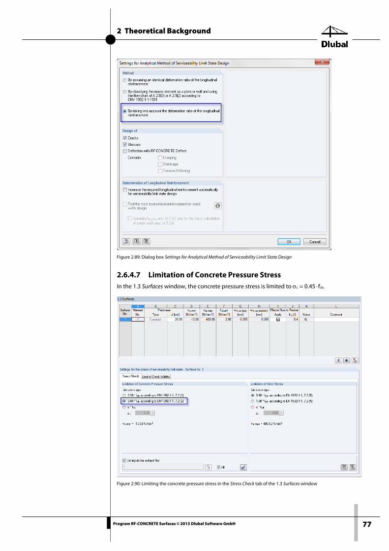
2 Theoretical Background
77 Program RF-CONCRETE Surfaces © 2013 Dlubal Software GmbH
Figure 2.89: Dialog box Settings for Analytical Method of Serviceability Limit State Design
2.6.4.7 Limitation of Concrete Pressure Stress In the 1.3 Surfaces window, the concrete pressure stress is limited to σc = 0.45 · fck.
Figure 2.90: Limiting the concrete pressure stress in the Stress Check tab of the 1.3 Surfaces window

2 Theoretical Background
78 Program RF-CONCRETE Surfaces © 2013 Dlubal Software GmbH
For concrete C30/37, the minimum concrete stress is determined as σc,min:
2ckmin,c mm/N5.130.3045.0f45.0 −=−⋅=⋅=σ
The provided concrete pressure stress is determined under the assumption of a linear stress distribution because the great number of iterations to determine the suitable direction of the concrete strut would be too time-consuming. A linear distribution is sufficiently exact because there are usually negative strains of maximum 0.3 to 0.5 ‰ in the SLS.
The minimum stress σc,min is to be compared to the provided stress of the concrete compres-sion zone for both directions of reinforcement.
The provided concrete pressure stress σc is determined as follows:
xI
m
II,i
Edc ⋅=σ
Equation 2.66
where
mEd Applied moment
2se
3II,i )xd(axb
31
I −⋅⋅α+⋅⋅= Ideal moment of inertia in the state II
B width of (for plates always 1 m)
αE Ratio of the elastic moduli
as Provided tension reinforcement
d Statically effective depth
⋅α⋅⋅
++−⋅⋅α
=se
se
adb0.2
0.10.1b
ax Depth of the concrete neutral axis
For direction of reinforcement ф, we obtain the following depth of neutral axis x-z,ф1 1:
cm19.431.11061.6171000.2
0.10.1100
31.11061.6x 1,z =
⋅⋅⋅
++−⋅⋅
=φ−
The same value and the according intermediate values can also be found in the details table.
Figure 2.91: Depth of the neutral axis for reinforcement direction 1

2 Theoretical Background
79 Program RF-CONCRETE Surfaces © 2013 Dlubal Software GmbH
For the reinforcement direction ф, we obtain the depth of neutral axis x-z,ф2 2:
cm02.431.11061.6
8.151000.20.10.1
10031.11061.6
x 2,z =
⋅⋅⋅
++−⋅⋅
=φ−
This value and the according intermediate values can also be read in the details.
Figure 2.92: Depth of the neutral axis for reinforcement direction 2
For the two directions of reinforcement, the ideal moments of inertia Ii,II in the state II (cracked section) are determined as follows:
4231,z,II,i cm13701)19.417(31.11061.619.40.100
3
1I =−⋅⋅+⋅⋅=φ−
4232,z,II,i cm11678)02.48.15(31.11061.602.4100
3
1I =−⋅⋅+⋅⋅=φ−
For the two directions of reinforcement ф1 and ф2, we obtain according to Equation 2.66 the following concrete pressure stresses σc in the concrete compression zone (i.e. the top surface):
21,o,c mm/N24.11
1370119.43676
−=⋅
=σ φ
22,o,c mm/N41.9
1167802.42733
−=⋅
=σ φ
These values are also shown in Figure 2.92.
Therefore, the existing compressive stresses σc,+z,ф1 and σc,+z,ф2 are smaller than the minimum con-crete stress σc,min (see Figure 2.90, page 77). The governing quotient of existing and allowable con-crete compressive stress is in the direction of reinforcement ф1. The design criterion is satisfied.
Figure 2.93: Analysis of the concrete compression stress

2 Theoretical Background
80 Program RF-CONCRETE Surfaces © 2013 Dlubal Software GmbH
2.6.4.8 Limitation of the Reinforcing Steel Stress
In the 1.3 Surfaces window, according to EN 1992-1-1, clause 7.2(5), tension stresses of the rein-forcing steel are limited to σs,max = 0.8 · fyk (see Figure 2.90, page 77). For BSt 500 S (B), the maxi-mum steel stress σs,max is determined as:
2ykmax,s mm/N4005008.0f8.0 =⋅=⋅=σ
The maximum stress σs,max is to be compared to the provided tension stress for both directions of reinforcement.
The provided tension stress σs is determined as follows:
( )II,i
EdEs I
xdm −⋅⋅α=σ
Equation 2.67
where αE Relation of the elastic moduli (Es / Ecm)
mEd Applied moment
d Statically effective depth
⋅α⋅⋅
++−⋅⋅α
=se
se
adb0.2
0.10.1b
ax Depth of the concrete neutral axis
b Width of the element (for plates always 1 m)
as Provided tension reinforcement
2se
3II,i )xd(axb
31
I −⋅⋅α+⋅⋅= Ideal moment of inertia in the state II
With the values calculated in chapter 2.6.4.6, it is possible to determine the provided tension stresses σs,u,ф1 and σs,u,ф2 in the two reinforcement directions ф1 and ф2 as follows:
21,u,s mm/N18.208
13701)19.417(3674061.6
=−⋅⋅
=σ φ
22,u,s mm/N09.167
11677)02.48.15(2733061.6
=−⋅⋅
=σ φ
Figure 2.94: Maximum steel stresses in reinforcement directions 1 and 2

2 Theoretical Background
81 Program RF-CONCRETE Surfaces © 2013 Dlubal Software GmbH
Therefore, the existing tension stresses σs,-z,ф1 and σs,-z,ф2 are smaller than the maximum steel stress σs,max (see Figure 2.90, page 77). The governing quotient of existing and allowable steel stress is in the reinforcement direction ф1. The design criterion is satisfied.
Figure 2.95: Analysis of reinforcing steel stress
2.6.4.9 Minimum Reinforcement for Crack Control
The minimum reinforcement cross-section for the crack control is determined according to EN 1992-1-1, clause 7.3.2, equation (7.1).
s
cteff,ctcmin,s
Afkka
σ⋅⋅⋅
=
Equation 2.68
where
kc Coefficient which takes account of the stress distribution within the section im-mediately prior to cracking and of the change of the lever arm
k Coefficient which allows for the effect of non-uniform self-equilibrating stresses, which lead to a reduction of restraint forces
fct,eff Mean value of the tensile strength of the concrete effective at the time when the cracks may first be expected to occur
Act Area of concrete within tensile zone (i.e. part of the cross-section which is calcu-lated to be in tension just before formation of the first crack)
σs Absolute value of the maximum stress permitted in the reinforcement immedi-ately after formation of the crack
The maximum bar diameter фs* is determined according to EN 1992-1-1, clause 7.3.3 (2) de-pending on the actually provided diameter фs from the converted equation (7.6N).
( )dh2
hk
9.2
f crceff,ct*ss −⋅
⋅⋅⋅φ=φ
Equation 2.69
where
фs Adjusted maximum bar diameter
фs* Maximum bar diameter according to EN 1992-1-1, Table 7.2 (see Figure 2.96)
h Overall depth of cross-section
hcr Depth of the tensile zone immediately prior to cracking, considering the charac-teristic values of prestress and axial forces under the quasi-permanent combina-tion of actions
d Effective depth to centroid of outside reinforcement
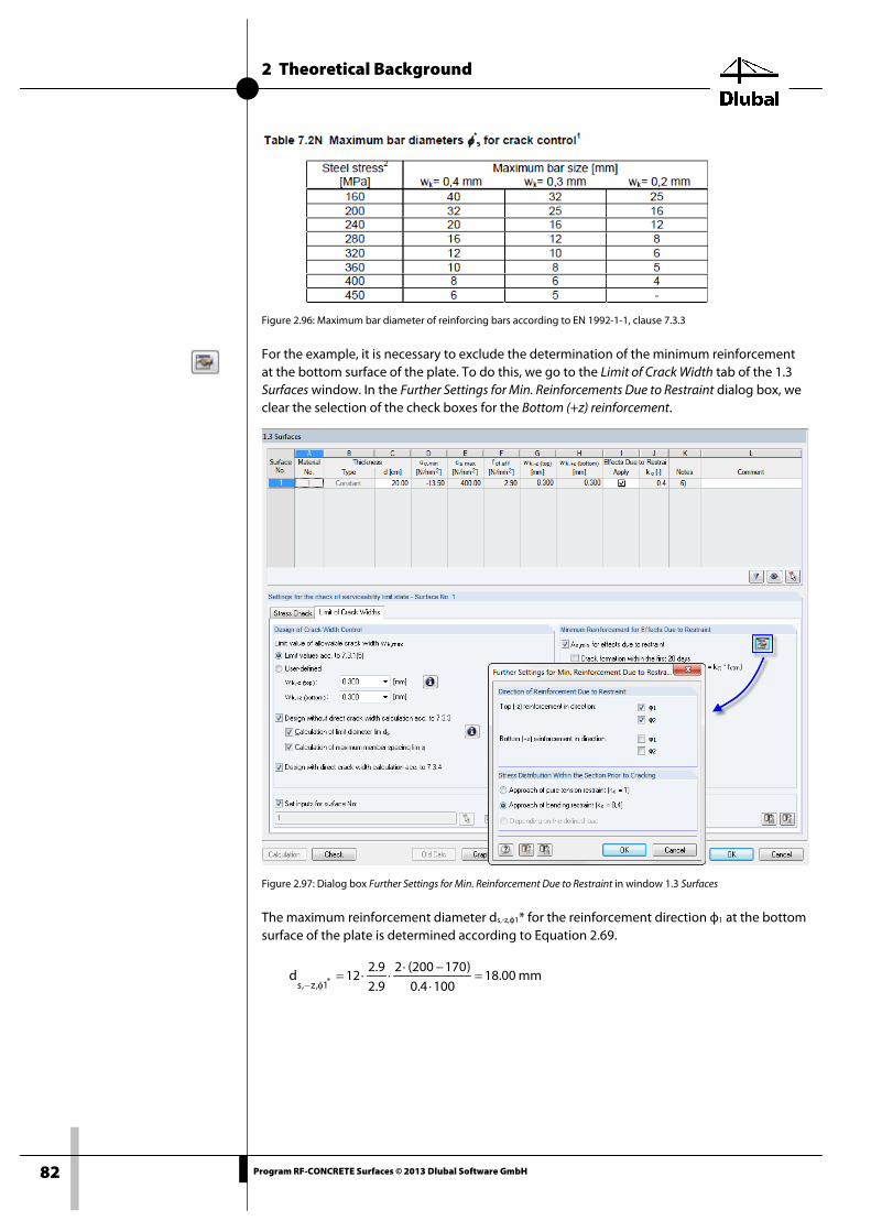
2 Theoretical Background
82 Program RF-CONCRETE Surfaces © 2013 Dlubal Software GmbH
Figure 2.96: Maximum bar diameter of reinforcing bars according to EN 1992-1-1, clause 7.3.3
For the example, it is necessary to exclude the determination of the minimum reinforcement at the bottom surface of the plate. To do this, we go to the Limit of Crack Width tab of the 1.3 Surfaces window. In the Further Settings for Min. Reinforcements Due to Restraint dialog box, we clear the selection of the check boxes for the Bottom (+z) reinforcement.
Figure 2.97: Dialog box Further Settings for Min. Reinforcement Due to Restraint in window 1.3 Surfaces
The maximum reinforcement diameter ds,-z,ф1* for the reinforcement direction ф1 at the bottom surface of the plate is determined according to Equation 2.69.
mm00.181004.0
)170200(29.29.2
12d *1,z,s=
⋅−⋅
⋅⋅=φ−
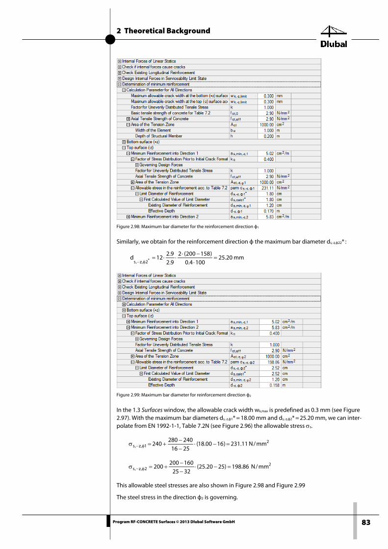
2 Theoretical Background
83 Program RF-CONCRETE Surfaces © 2013 Dlubal Software GmbH
Figure 2.98: Maximum bar diameter for the reinforcement direction ф1
Similarly, we obtain for the reinforcement direction ф the maximum bar diameter ds,-z,ф22* :
mm20.251004.0
)158200(29.29.2
12d *2,z,s=
⋅−⋅
⋅⋅=φ−
Figure 2.99: Maximum bar diameter for reinforcement direction ф2
In the 1.3 Surfaces window, the allowable crack width wk,max is predefined as 0.3 mm (see Figure 2.97). With the maximum bar diameters ds,-z,ф1* = 18.00 mm and ds,-z,ф2* = 25.20 mm, we can inter-polate from EN 1992-1-1, Table 7.2N (see Figure 2.96) the allowable stress σs.
21,z,s mm/N11.231)1600.18(
2516240280
240 =−⋅−−
+=σ φ−
22,z,s mm/N86.198)2520.25(
3225160200
200 =−⋅−−
+=σ φ−
This allowable steel stresses are also shown in Figure 2.98 and Figure 2.99
The steel stress in the direction ф2 is governing.

2 Theoretical Background
84 Program RF-CONCRETE Surfaces © 2013 Dlubal Software GmbH
The surface of the concrete compression zone in the cross-section is determined as follows:
2ct cm1000
220
1002h
bA =⋅=⋅=
According to the Equation 2.68 on page 81, we obtain for the reinforcement direction 2 the following minimum reinforcement:
m/cm83.586.198
10009.20.14.0a 2
2min,,s =⋅⋅⋅
=φ
For this reinforcement direction, the applied reinforcement is greater than the minimum rein-forcement. Thus we obtain the following design criterion:
516.031.11
83.5a
a
2,z,exist,s
2,zmin,,s ==−
−
Figure 2.100: Design criterion for minimum reinforcement
2.6.4.10 Checking the Rebar Diameter The maximum bar diameter of the rebars, max ds, is determined according to EN 1992-1-1, Equation (7.6N) (see Equation 2.69, page 81).
At the top surface of the plate, the program determines the maximum bar diameter d*s,-z,ф1 of the first reinforcement direction, depending on the stress in this direction. In the check of the limitation of the steel stress, this stress was computed with σs,-z,ф1 = 208.18 N/mm2. Together with the selected crack width wk = 0.3 mm, we obtain by interpolation in Table 7.2N the follow-ing maximum bar diameter d*s,-z,ф1 :
mm16.23)20018.208(2402001625
25d*1,z,s =−⋅
−−
+=φ−
Figure 2.101: Maximum bar diameter in reinforcement direction 1

2 Theoretical Background
85 Program RF-CONCRETE Surfaces © 2013 Dlubal Software GmbH
Similarly, the maximum bar diameter for the reinforcement direction 2 d*s,-z,ф2 is determined from the tension stress σs,-z,ф2 = 167.09 N/mm2 and the crack width wk = 0.3 mm:
mm76.30)16009.167(2001602532
32d*2,z,s =−⋅
−−
+=φ−
Figure 2.102: Maximum bar diameter in reinforcement direction 2
With the maximum bar diameters ds* for the two reinforcement directions and the respective steel stresses, the following maximum bar diameters ds are determined:
mm44.15)170200(2
1004.09.29.2
16.23d 1,zmax,,s =−⋅
⋅⋅⋅=φ−
mm65.14)158200(2
1004.09.29.2
76.30d 2,zmax,,s =−⋅
⋅⋅⋅=φ−
Figure 2.103: Maximum bar diameter
For both reinforcement directions, the bar diameter ds = 12 mm is specified, respectively. Thus, we obtain the design criterion for the governing reinforcement direction ф1:
819.065.140.12
dmax
d
2,z,s
2,z,exist,s ==φ−
φ−
Figure 2.104: Design criterion for bar diameter

2 Theoretical Background
86 Program RF-CONCRETE Surfaces © 2013 Dlubal Software GmbH
2.6.4.11 Design of Rebar Spacing In the Longitudinal Reinforcement tab of the 1.4 Reinforcement window, we clicked the [Rebars] button, and specified a rebar spacing of a = 100 mm for both reinforcement directions in the Import Reinforcement Area Due to Rebar dialog box (see Figure 2.84, page 74).
Figure 2.105: Dialog box Import Reinforcement Area due to Rebar
The maximum rebar spacing sl,-z,ф1 is determined by interpolation according to EN 1992-1-1, Ta-ble 7.3N for the existing tension stress σs,-z,ф1 = 208.18 N/mm2 and the crack width wk = 0.3 mm.
Figure 2.106: Maximum values for rebar spacing according to EN 1992-1-1, Table 7.3N
mm8.239)20018.208(240200
200250250smax 1,z,l =−⋅
−−
+=φ−
Similarly, the maximum bar spacing for the direction ф2 is determined from the existing tension stress σs,-z,ф2 = 167.09 N/mm2 as max sl,-z,ф2 = 291.1 mm.
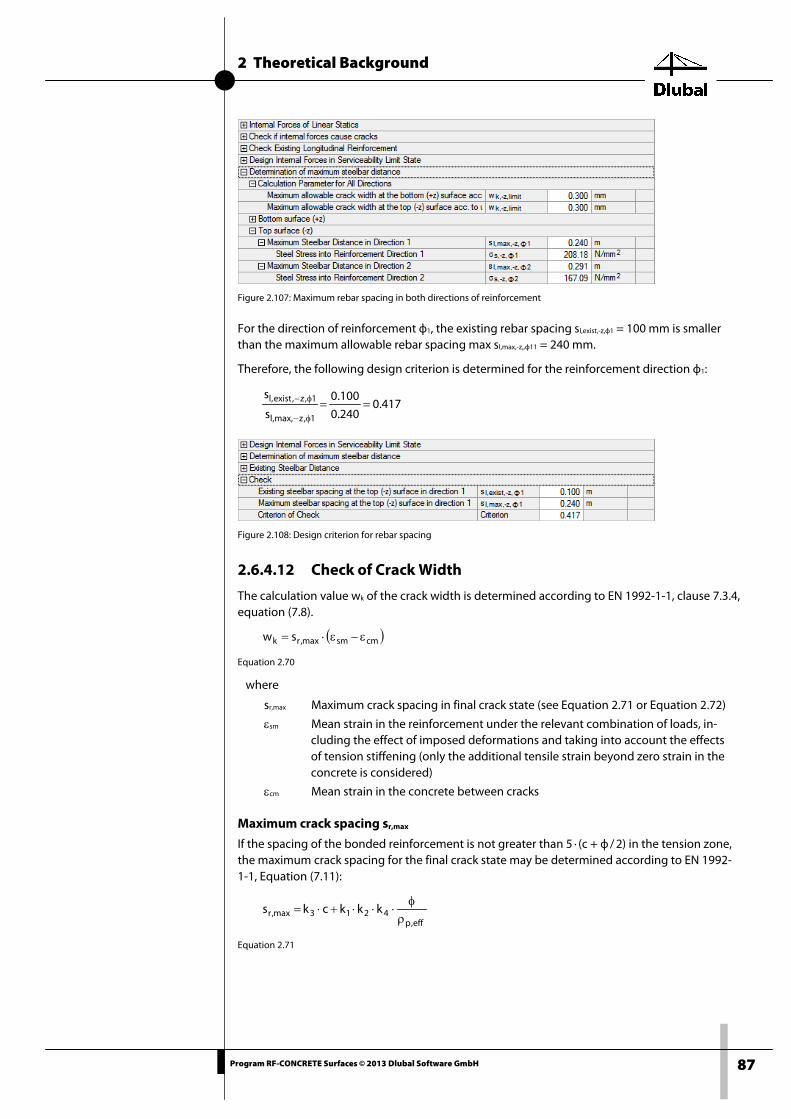
2 Theoretical Background
87 Program RF-CONCRETE Surfaces © 2013 Dlubal Software GmbH
Figure 2.107: Maximum rebar spacing in both directions of reinforcement
For the direction of reinforcement ф1, the existing rebar spacing sl,exist,-z,ф1 = 100 mm is smaller than the maximum allowable rebar spacing max sl,max,-z,,ф11 = 240 mm.
Therefore, the following design criterion is determined for the reinforcement direction ф1:
417.0240.0
100.0
s
s
1,zmax,,l
1,z,exist,l ==φ−
φ−
Figure 2.108: Design criterion for rebar spacing
2.6.4.12 Check of Crack Width
The calculation value wk of the crack width is determined according to EN 1992-1-1, clause 7.3.4, equation (7.8).
( )cmsmmax,rk sw ε−ε⋅=
Equation 2.70
where
sr,max Maximum crack spacing in final crack state (see Equation 2.71 or Equation 2.72)
εsm Mean strain in the reinforcement under the relevant combination of loads, in-cluding the effect of imposed deformations and taking into account the effects of tension stiffening (only the additional tensile strain beyond zero strain in the concrete is considered)
εcm Mean strain in the concrete between cracks
Maximum crack spacing sr,max
If the spacing of the bonded reinforcement is not greater than 5 · (c + ф / 2) in the tension zone, the maximum crack spacing for the final crack state may be determined according to EN 1992-1-1, Equation (7.11):
eff,p4213max,r kkkcks
ρφ
⋅⋅⋅+⋅=
Equation 2.71

2 Theoretical Background
88 Program RF-CONCRETE Surfaces © 2013 Dlubal Software GmbH
If the rebar spacing in the bonded reinforcement exceeds 5 · (c + ф / 2), or if no bonded rein-forcement is available within the tension zone, the limit for the crack width may be deter-mined with the following crack spacing:
( )xh3.1s max,r −⋅=
Equation 2.72
Therefore, the depth of the neutral axis x in state II is to be calculated for the check of the crack width. It is determined with the depth of the structural member related to the depth of the neutral axis ξ.
h
hb
a0.1
hd
hb
a5.0
hxexist,s
e
exist,se
⋅
⋅⋅α+
⋅⋅
⋅α+=⋅ξ=
Equation 2.73
Figure 2.109: Maximum crack spacing in reinforcement direction 1
Furthermore, the maximum crack width is analyzed according to EN 1992-1-1, equation (7.15):
ymax,,rxmax,,r
max,r
ssin
scos
1s
θ+
θ=
Equation 2.74
where
θ Angle between the reinforcement in x-direction and the principal tension stress
sr,max,x, sr,max,y Maximum crack spacing in y- or z-direction
This equation is important if in the dialog box Settings for Analytical Method of Serviceability Lim-it State Designs (see Figure 2.89, page 77) the first method By assuming an identical deformation

2 Theoretical Background
89 Program RF-CONCRETE Surfaces © 2013 Dlubal Software GmbH
ratio of the longitudinal reinforcement has been selected to determine the design internal forces in the serviceability limit state. In the third method (By taking into account the deformation ratio of the longitudinal reinforcement), on the other hand, the direction of the concrete strut is deter-mined according to BAUMANN. The limit angle of 15° is ignored since the crack width in this area is not governing.
Figure 2.110: Maximum crack spacing for both reinforcement directions
Difference of mean strain (εsm - εcm)
For the calculation value of the crack width wk according to Equation 2.70 on page 87, we now need to determine the factor (εsm – εcm) for each direction of the resulting strain.
The difference of mean strain for concrete and reinforcing steel is determined in accordance with EN 1992-1-1, 7.3.4, Eq. (7.9):
( )
s
s
s
effeeff
eff,ctts
cmsm E6.0
E
1f
kσ
⋅≥ρ⋅α+⋅
ρ⋅−σ
=ε−ε
Equation 2.75
The maximum mean strain (εsm − εcm)-z,res is obtained as the resulting mean strain of the individ-ual reinforcement directions and is 1.291 ‰.
Figure 2.111: Difference of the mean strain for both reinforcement directions

2 Theoretical Background
90 Program RF-CONCRETE Surfaces © 2013 Dlubal Software GmbH
To make the expression clearer, we introduce symbols for the sought mean strain (εsm− εcm): s for the side length in the direction of the reinforcement, d for the partial length of the con-crete struts, l for the perpendicular to the concrete strut, and ε.
Figure 2.112: Mean strain ε
The partial length dγ-α is determined for a selected inclination of the concrete strut as follows:
( )α−γ=α−γ tan
1d
The length is unitless (the perpendicular to the concrete strut is included without unit).
Then, the length sγ-α is determined.
( )α−γε+
= αα−γ sin
1s
If the reinforcement direction θ1 forms the smallest differential angle with the principal mo-ment m1, then for εα we have to insert the previously determined difference of the mean strains (εsM − εcm)θ1 of concrete and reinforcing steel:
( )( )α−γ
ε−ε+= θ
α−γ sin
1s 1cmsm
If the reinforcement direction θ1 forms the smallest differential angle with the principal mo-ment m1, then for εα we have to insert the previously determined difference of the mean strains (εsm − εcm)θ2 2 of concrete and reinforcing steel:
With the Pythagorean theorem, we can determine the value lγ-α from the lengths dγ-α and sγ-α:
22 dsl α−γα−γα−γ −=
Since all formulas are based on an initial length of 1.0 units of length, the strain ε is determined as follows:
0.1l −=ε α−γ
This strain ε = (εsM − εcm) is checked again by means of the intermediate angle (β - γ).
For the determination of the SLS design internal forces according to the method By assuming an identical deformation ratio of the longitudinal reinforcement, the deformation ratio of the reinforcements can significantly deviate from the assumed geometric deformation ratio. To determine the resulting deformation ratio correctly, the program uses the strain of the rein-forcement that is closer to the main action.

2 Theoretical Background
91 Program RF-CONCRETE Surfaces © 2013 Dlubal Software GmbH
Crack width wk
The calculated value of the crack width wk is determined according to Equation 2.70, page 87.
Figure 2.113: Calculation value of crack width
In the 1.3 Surfaces window, we specified the maximum allowable crack width max wk = 0.3 mm. Thus, we obtain the design criterion for the governing resulting direction.
Figure 2.114: Design criterion for crack width
2.6.5 Governing Effects of Actions In RFEM, it is possible to define the various loadings in the individual load cases (LC). Load cas-es can be superimposed in load combinations (CO) and result combinations (RC). The differ-ence between both types of combinations is described in chapters 5.5 and 5.6 of the RFEM manual.
Load cases and load combinations yield only one set of internal forces, respectively. In a result combination, however, there can be up to 16 sets of internal forces, depending on the type of model:
• For the types of model 2D - XZ (uX/uZ/φY) and 2D - XY (uX/uY/φZ) (wall), we obtain only the axial forces nx, ny, and nxy in the surfaces. Their combination yields six sets of internal forc-es, of which one of these axial forces shows its maximum or minimum value, respectively.
• For the type of model 2D - XY (uZ/φX/φY) (plate), the maximum and minimum values of the moments mx, my, and mxy as well as their shear forces vx and vy are determined. Thus, we obtain ten sets of internal forces.
• The type of model 3D contains all the axial forces, moments, and shear forces mentioned above and, therefore, yields 16 sets of internal forces.
The analysis core for the serviceability limit state designs proceeds with the internal forces of the selected load cases and load combinations sequentially, that is, row by row. The same is true for the sets of internal forces of a result combination. This shows that the design of a result combination is much more time-consuming.
In most checks for the individual reinforcement directions, the internal forces or sets of internal forces result in an action-effect. The program determines the greatest action-effect of all rein-forcement directions. If the resistance for the individual reinforcement directions is different, the program searches for the reinforcement direction that yields the greatest quotient from action-effect over resistance.

2 Theoretical Background
92 Program RF-CONCRETE Surfaces © 2013 Dlubal Software GmbH
2.7 Deformation analysis with RF-CONCRETE Deflect
For the deformation analysis, you need a license of the RF-CONCRETE Deflect add-on module.
2.7.1 Basic Material and Geometric Assumptions For the deformation analysis with RF-CONCRETE Deflect, a linear-elastic compression and ten-sion behavior of reinforcing steel is assumed. Here, a linear-elastic compression behavior and a linear-elastic behavior is applied until the tension strength is reached. Such assumptions are sufficiently exact for the serviceability limit state. If the provided stress exceeds the concrete strength, damage develops according to EN 1992-1-1, clause 7.3.4.
The calculation uses a simple isotropic model of fracture mechanics that is defined individually in the two directions of reinforcement. From an engineering point of view, in accordance with EN 1992-1-1, a material stiffness matrix is computed by interpolation between the uncracked (state I) and cracked state (state II) according to clause 7.4.3, Equation (7.18). Thus, the rein-forced concrete is modeled as an orthotropic material. All laws of the damage development can take into account the tension stiffening effect and simple long-term effects (shrinkage and creep).
The computation of the material stiffness matrices is implemented for the types of model 2D - XY (uZ/φX/φY) and 3D. For the 3D type of model, the influence of the eccentricities of the ideal centroids (see below) is additionally considered in the stiffness matrix.
2.7.2 Design Internal Forces As described above, the calculation of stiffnesses is based on linear-elastic assumptions. The internal forces are transformed in the orthogonal direction of reinforcements ф and to the two surfaces s (top and bottom). The obtained internal forces – bending moments mф.s and axial forces nф.s (torsion moments are eliminated by a transformation in the directions of reinforce-ment) – depend on the
(a) type of model
(b) method of calculation
(c) classification criterion.
2.7.3 Critical Surface For the determination of the critical surface, each reinforcement direction ф is considered sep-arately. The state of stress is analyzed on both surfaces s – bottom surface (in the direction of the local +z-axis) and top surface (in the direction of the local -z-axis). The surface with the greater tension in concrete is classified as governing. The internal forces on the critical surfaces are termed nф and mф.
The axial force nф.s transformed in the direction of reinforcement ф has the same value for both surfaces s (nф = nф,top = nф,bottom). Therefore, the axial forces are not relevant for the determina-tion of the critical surface; only the moments are considered in order to find the governing sur-face. The signs for the bending moments mф,s are determined regarding whether the moments cause tension or compression on the corresponding surface, respectively. Therefore, the criti-cal surface is that with the greater bending moment (that is, the surface that is more subjected to tension).
For the calculation of the stiffness, only the internal forces nф and mф on the critical surface are taken into account. Until now, the term "bottom surface" referred to the local +z-axis. In the following, however, "bottom surface" refers to the critical side of the surface.
2 Theoretical Background
93 Program RF-CONCRETE Surfaces © 2013 Dlubal Software GmbH
2.7.4 Cross-Section Properties The cross-section properties are determined for both reinforcement directions and for both cross-section states c (cracked / uncracked). For state I (uncracked cross-section), a linear-elastic behavior of concrete in tension is applied. For state II (cracked cross-section), the tensile strength of concrete is not applied.
If there are no axial forces nф (for example in the type of model 2D - XY (uZ/φX/φY)), this part of the computation is independent of internal forces and a direct calculation of the cross-section properties is possible. In the other cases, the depth of the neutral axis is calculated by means of an iterative method of calculation, the so-called "binary method." For numerical reasons, the program uses the minimum value for the reinforcement ratio ρmin = 10−4 in every iteration step. That is, if there is no reinforcement, a virtual minimum reinforcement area is applied. Such a small value has no appreciable influence on the results (stiffnesses).
The calculated ideal cross-section properties (related to the concrete cross-section) in a rein-forcement direction ф and the crack state c are the:
(a) moment of inertia to the ideal center of gravity Iф,c
(b) moment of inertia to the geometric center of the cross-section I0.ф,c
(c) cross-section area Aф,c
(d) eccentricity of the ideal center of gravity eф,c .
2.7.5 Long-Term Effects Shrinkage and creep are time-dependent properties of concrete. According to EN 1992-1-1, the long-term effects are to be considered separately.
2.7.5.1 Creep The creep effects are considered by reduction of the concrete modulus of elasticity E, using the effective creep coefficient φeff according to EN 1992-1-1, Equation (7.20):
eff
cdeff,cd 1
EE
ϕ+=
Equation 2.76
2.7.5.2 Shrinkage In the deflection calculation according to EN 1992-1-1, there are two topics that are influenced by shrinkage effects.
Reduction of material stiffness
The material stiffness in each reinforcement direction ф is reduced by a so-called coefficient of shrinkage influence ksh.ф,c. For both crack states c (cracked / uncracked), the axial forces nsh.ф,c
and bending moments msh.ф,c are determined from the free shrinkage strain εsh:
( )2s1sssh,sh aaEn +⋅ε−=φ
shsh,sh enm ⋅=φ
Equation 2.77
where
nsh,ф Additional axial force from shrinkage in reinforcement direction ф
msh,ф Additional moment from shrinkage in center of gravity of the ideal cross-section in the direction of reinforcement ф
aS1 Bottom surface of reinforcement
aS2 Top surface of reinforcement
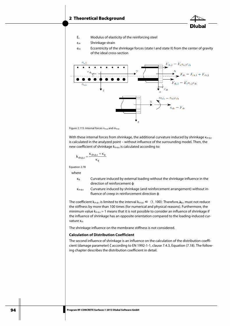
2 Theoretical Background
94 Program RF-CONCRETE Surfaces © 2013 Dlubal Software GmbH
Es Modulus of elasticity of the reinforcing steel
εsh Shrinkage strain
esh Eccentricity of the shrinkage forces (state I and state II) from the center of gravity of the ideal cross-section
Figure 2.115: Internal forces nsh,ф and msh,ф
With these internal forces from shrinkage, the additional curvature induced by shrinkage κsh.ф,c is calculated in the analyzed point – without influence of the surrounding model. Then, the new coefficient of shrinkage ksh.ф,c is calculated according to:
φ
φφφ κ
κ+κ= c,,sh
c,,shk
Equation 2.78
where
κф Curvature induced by external loading without the shrinkage influence in the direction of reinforcement ф
κsh.ф.c Curvature induced by shrinkage (and reinforcement arrangement) without in-fluence of creep in reinforcement direction ф
The coefficient ksh.ф.c is limited to the interval ksh.ф.c ∈ (1, 100): Therefore, ksh.ф.c must not reduce the stiffness by more than 100 times (for numerical and physical reasons). Furthermore, the minimum value ksh.ф.c = 1 means that it is not possible to consider an influence of shrinkage if the influence of shrinkage has an opposite orientation compared to the loading-induced cur-vature κd.
The shrinkage influence on the membrane stiffness is not considered.
Calculation of Distribution Coefficient
The second influence of shrinkage is an influence on the calculation of the distribution coeffi-cient (damage parameter) ζ according to EN 1992-1-1, clause 7.4.3, Equation (7.18). The follow-ing chapter describes the distribution coefficient in detail.
2 Theoretical Background
95 Program RF-CONCRETE Surfaces © 2013 Dlubal Software GmbH
2.7.6 Distribution Coefficient The calculation of the distribution coefficient ζd is shown for reinforcement direction ф. First, the program calculates the maximum concrete tension stress σmax.ф under the assumption of a linear-elastic material behavior:
( )I,I,
I,,shI,
I,
,shmax, xh
I
m2h
xnm
A
nnφ
φ
φφφφ
φ
φφφ −⋅
+
−⋅−
++
=σ
Equation 2.79
where
nф Axial force from external loading in reinforcement direction ф
nsh,ф Additional axial force from shrinkage in reinforcement direction ф
mф Moment from external loading in reinforcement direction ф
msh,ф,I Additional moment from shrinkage in reinforcement direction ф in state I
xф,I Depth of neutral axis in uncracked state in reinforcement direction ф
h Depth of the cross-section
Aф.I Ideal cross-section area in state I in reinforcement direction ф
Iф.I Ideal moment of inertia in state I in reinforcement direction ф
The influence of shrinkage force on the maximum tension stress σmax.ф is considered with the additional internal forces from shrinkage.
The calculation of the distribution coefficient ζ ф depends on whether the tension stiffening according to EN 1992-1-1 is taken into account in the deformation calculation.
Distribution coefficient ζ ф taking into account tension stiffening
• for σmax.ф > fctm :
n
max,
ctmf1
σ⋅β−=ζ
φφ
• for σmax.ф ≤ fctm :
0=ζφ
Equation 2.80
where
β Parameter to taken into account the load duration
fctm Mean tensile strength
n 2 for EN 1992-1-1
Coefficient of distribution ζ ф without consideration of tension stiffening
• for σmax.ф > fctm :
1=ζφ
• for σmax.ф ≤ fctm :
0=ζφ
Equation 2.81
2 Theoretical Background
96 Program RF-CONCRETE Surfaces © 2013 Dlubal Software GmbH
2.7.7 Cross-Section Properties for Deformation Analysis In the material stiffness matrix D for the deformation analysis, the program requires the cross-section properties available in every direction of reinforcement depending on the cracked state. These are the following:
(a) moment of inertia to the ideal center of gravity Iф
(b) moment of inertia to the geometric center of cross-section I0.c
(c) ideal cross-section area Aф
(d) eccentricity of the ideal center of gravity eф to the geometric center.
A mean strain ε ф and a mean curvature κ ф are computed as interpolation between a cracked and an uncracked state according to EN 1992-1-1, Equation (7.18):
( ) I,II, 1 φφφφφ ε⋅ζ−+ε⋅ζ=ε
( ) I,II, 1 φφφφφ κ⋅ζ−+κ⋅ζ=κ
Equation 2.82
The strain in the cracked state c (state I and II) are computed according to the following equa-tions:
c,c, AE
n
φ
φφ ⋅
=ε
c,
c,c,,shc, IE
enm
φ
φφφφφ ⋅
⋅−⋅κ=κ
Equation 2.83
The influence of the shrinkage is considered by using factor ksh.ф.c.
If there are no axial forces nф (for example in the type of model 2D - XY (uZ/φX/φY)), only those ideal cross-section properties are relevant that relate to the ideal center of the cross-section:
( ) I,,shII,II,,shI,
II,I,
kA1kA
AAA
φφφφφφ
φφφ ⋅⋅ζ−+⋅⋅ζ
⋅=
( ) I,,shII,II,,shI,
II,I,
kI1kI
III
φφφφφφ
φφφ ⋅⋅ζ−+⋅⋅ζ
⋅=
Equation 2.84
If axial forces are available, the cross-section properties are related to the geometric center of cross-section:
φ
φφ ε⋅
=A
nA where
φ
φφφφ
⋅⋅κ−=ε
n
IEm
20, eAII φφφφ ⋅+= where Iф according to Equation 2.84
Equation 2.85
In the calculation of the cross-section properties, the initial value of the poisson's ratio νinit is reduced according to the following equation:
( )( ) init2,1max1 ν⋅ζ−=ν φ∈φ
Equation 2.86

2 Theoretical Background
97 Program RF-CONCRETE Surfaces © 2013 Dlubal Software GmbH
2.7.8 Material Stiffness Matrix D
Bending stiffness - plates and shells The bending stiffnesses in the directions of reinforcement ф are determined as follows:
Dd,d = I0,d · E / (1- ν2 ) where d = 1,2
Dd,d = Id · E / (1- ν2 ) where d = 1,2
The non-diagonal component of the material stiffness matrix has the same expression for plates and shells:
D1,2 = D2,1 = ν · √(D1,1·D2,2)
For shells, the differences in the bending stiffnesses due to the moments of inertia are com-pensated by the eccentricity components in the material stiffness matrix.
Torsion stiffness of plates and shells The elements of the stiffness matrix are calculated for plates and shells as follows:
D3,3 = (1-ν)/2 · √(D1,1·D2,2)
Shear stiffness of plates and shells The elements of the stiffness matrix for shear are not reduced for the deformation analysis. They are determined from the shear modulus G of the ideal cross-section and the cross-section height h. The expression for shells and plates is the same:
D3+d,3+d = 5/6 · Gh where d = 1,2
Membrane stiffness of shells The membrane stiffnesses in the reinforcement directions ф are determined as follows:
Dd+5,d+5 = E·Ad / (1- ν2) where d = 1,2
The non-diagonal part of the material stiffness matrix is determined from:
D6,7 = D7,6 = ν · √(D6,6 · D7,7)
The part of the shear stiffness component is:
D8,8 = G· h
Eccentricity – shells The elements of the stiffness matrix for the eccentricity of the centroid (ideal cross-section) in the reinforcement direction ф are determined as follows:
Dd,6 = D6,d = Dd+5,d+5 · ed where d = 1,2
The non-diagonal component of the material stiffness matrix is determined from:
D1,7 = D7,1 = ν/2 · (eΦ1 + eΦ2) · √(D6,6 · D7,7)
The eccentricity components for torsion are determined as follows:
D3,8 = D8,3 = 1/2 · G·h·(eΦ1 + eΦ2)
2.7.9 Positive Definite Test The positive definite of the material stiffness matrix D is tested by a modified (with respect to the blocks of zeros) SYLVESTER'S criterion. If the stiffness matrix D is not positive definite, the non-diagonal components of the material stiffness matrix are zeroed consecutively. In the extreme case, only the positive components from the diagonal remain.

2 Theoretical Background
98 Program RF-CONCRETE Surfaces © 2013 Dlubal Software GmbH
2.7.10 Example The determination of the material stiffness matrix D is illustrated by a simple example. The model contains only one finite element and the surface is reinforced only on one side (top). For simplicity's sake, the manual calculation is carried out in the reinforcement direction ф1.
2.7.10.1 Geometry The model with the dimensions 1 x 1 m and the thickness 0.20 m is fixed at one side. The free side is subjected to the bending moment mx = - 30 kNm/m and the axial force nx = - 100 kN/m. The automatic self-weight is not taken into account.
The longitudinal reinforcement in ф1 is 1000 mm2.
Figure 2.116: Model with loading and reinforcement
2.7.10.2 Materials The following table shows the material properties.
Figure 2.117: Material data for stiffness calculation
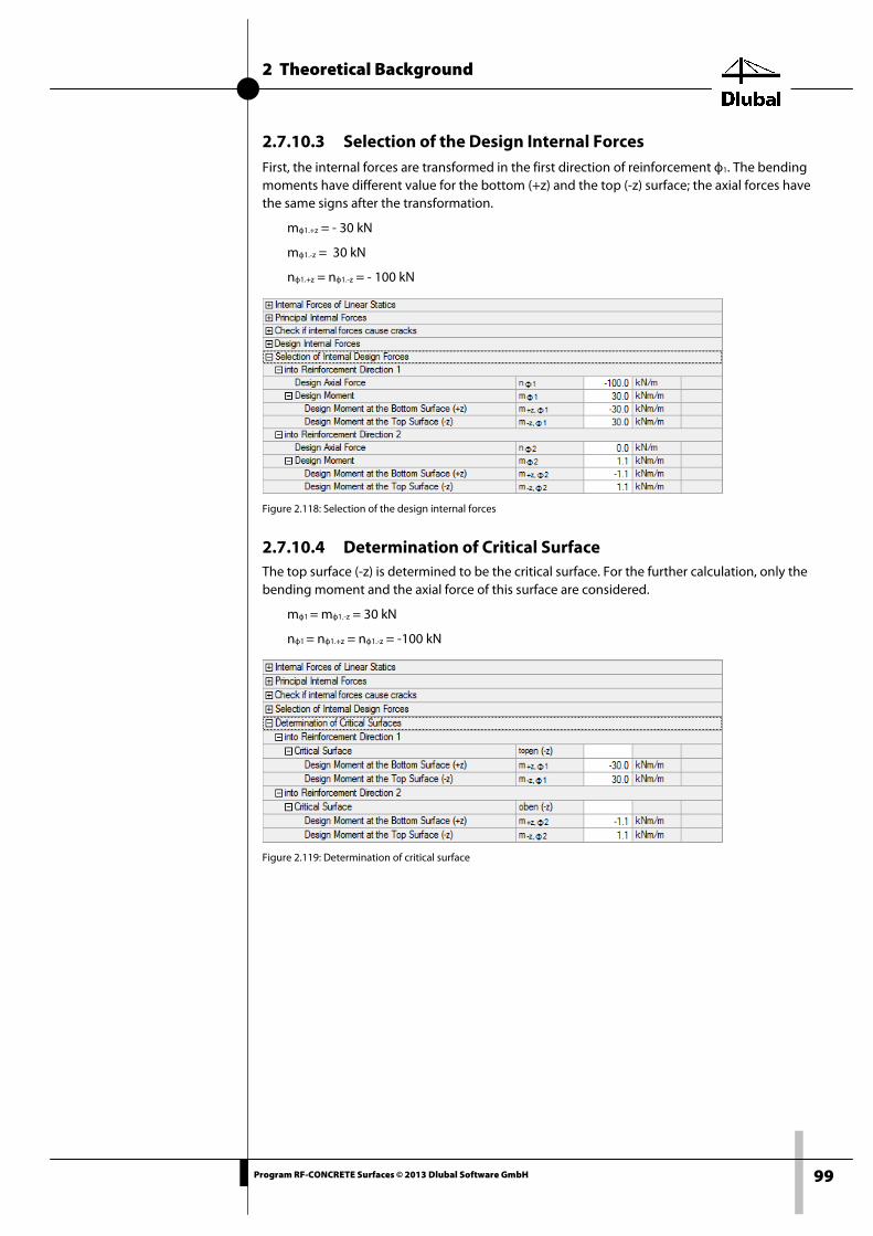
2 Theoretical Background
99 Program RF-CONCRETE Surfaces © 2013 Dlubal Software GmbH
2.7.10.3 Selection of the Design Internal Forces First, the internal forces are transformed in the first direction of reinforcement ф1. The bending moments have different value for the bottom (+z) and the top (-z) surface; the axial forces have the same signs after the transformation.
mф1.+z = - 30 kN
mф1.-z = 30 kN
nф1.+z = nф1.-z = - 100 kN
Figure 2.118: Selection of the design internal forces
2.7.10.4 Determination of Critical Surface The top surface (-z) is determined to be the critical surface. For the further calculation, only the bending moment and the axial force of this surface are considered.
mф1 = mф1.-z = 30 kN
nф1 = nф1.+z = nф1.-z = -100 kN
Figure 2.119: Determination of critical surface

2 Theoretical Background
100 Program RF-CONCRETE Surfaces © 2013 Dlubal Software GmbH
2.7.10.5 Cross-Section Properties (Cracked and Uncracked State) The cross-section properties depend on the governing surface and the direction of reinforce-ment ф1. The minimum values are used for the surfaces of reinforcement as2,ф1 , as1,ф2, and as2,ф2.
The following cross-section properties for the uncracked and cracked state are to be calculated in order to be able to assemble the stiffness matrix of the material D.
Center of gravity
The distance of the center of gravity of the ideal cross-section from the concrete surface in compression is directly determined for the uncracked state.
( )
( )1,2s1,1s
1,21,2s1,11,1s
2
1,I aahb
dada2hb
zφφ
φφφφ
φ +⋅α+⋅
⋅+⋅⋅α+⋅
=
( )( )151000061.62001000
50151501000061.62
2001000 2
+⋅+⋅
⋅+⋅⋅+⋅
= = 101.4 mm
For the cracked state, the depth χII,ф 1 of the zone in compression must be calculated iteratively. The distance of the center of gravity of the ideal cross-section from the surface in compression is calculated for the cracked state.
Ideal cross-section area Ac,d
The effective cross-section area in the uncracked state without the influence of creep is:
AI.ф1 = b · h + α · (as1.ф1 + as2.ф1) = 1000 · 200 + 6.061· (1000 + 15) = 2061.5cm2
The effective cross-section area in the cracked state is determined with the influence of creep.
AII.ф1 = b · χII.ф1 + α · (as1.ф1 + as2.ф1) = 1000 · 68.3 + 18.182 · (1000 + 15) = 867.19 cm2
The coefficient α is the ratio of the moduli of elasticity of steel and concrete with or without the influence of creep.
Ideal moment of inertia to ideal center of gravity Ic,d
The effective moment of inertia to the ideal center of gravity in the uncracked state without in-fluence of creep is:
II.ф1 = 1/12·· h3 + bb · h · (zI.ф1 - h/2)2 + α · as1.ф1 · (d1.ф1 - zI,ф1)2 + α · as2.ф1 · (zI.ф1 - d2,ф1)2
= 1/12·1000·2003 + 1000·200·(101.4-200/2)2 + 6.061·1000·(150-101.4)2 + 6.061·15·(101.4-50)2
= 68,161.30 cm4
The effective moment of inertia to the ideal center of gravity in the cracked state is determined with the influence of creep.
III.ф1 = 1/12·· 3
II.ф1 + bb · χII.ф1 · (zII.ф1 - χχII.ф1/2)2 + α · as1.ф1 · (d1.ф1 - zII,ф1)2 + α · as2.ф1 · (zII.ф1 - d2,ф1)2
= 1/12·1000·68.33 + 1000·68.3·(58.5- 68.3/2)2
+ 18.182·1000·(150-58.5)2 + 18.182·15·(58.5-50)2
= 21,928.70 cm4
Ideal moment of inertia to geometric center of cross-section I0,c,d
The ideal moment of inertia to the geometric center of the cross-section in the uncracked state without influence of creep is:
I0.I.ф1 = 1/12· b· h3 + α ·as1.ф1 · (d1.ф1 - h/2)2 + α · as2.ф1 · (h/2 - d2,ф1)2
= 1/12·1000·2003 + 6.061·200·(150 - 200/2)2 + 6.061·15·(200/2 - 50)2
= 68,204.50 cm4

2 Theoretical Background
101 Program RF-CONCRETE Surfaces © 2013 Dlubal Software GmbH
The ideal moment of inertia to the geometric center of the cross-section in the cracked state is determined from the influence of creep.
I0.II.ф1 = 1/12· · χ3II.ф1 + bb · χII.ф1 · (h/2 - χII.ф1/2)2 + α · as1.ф1 · (d1.ф1 - h/2)2 + α · as2.ф1 · (h/2 - d2,ф1)2
= 1/12·1000·68.33 + 1000·68.3·(200/2 - 68.3/2)2 + 18.182·1000·(150 - 200/2)2 + 18.182·15· (200/2-50)2
= 36,881.50 cm4
Eccentricity of the centroid ec,d
The eccentricity of the ideal center of gravity is determined as follows:
ec,ф1 = zc,ф1 – h/2
• Uncracked state:
eф1.I = 101.4 – 200/2 = 1.4 mm
• Cracked state:
eф1.II = 58.5 – 200/2 = - 41.5 mm
Figure 2.120: Cross-sectional properties in reinforcement direction 1
Figure 2.121: Cross-sectional properties in reinforcement direction 2
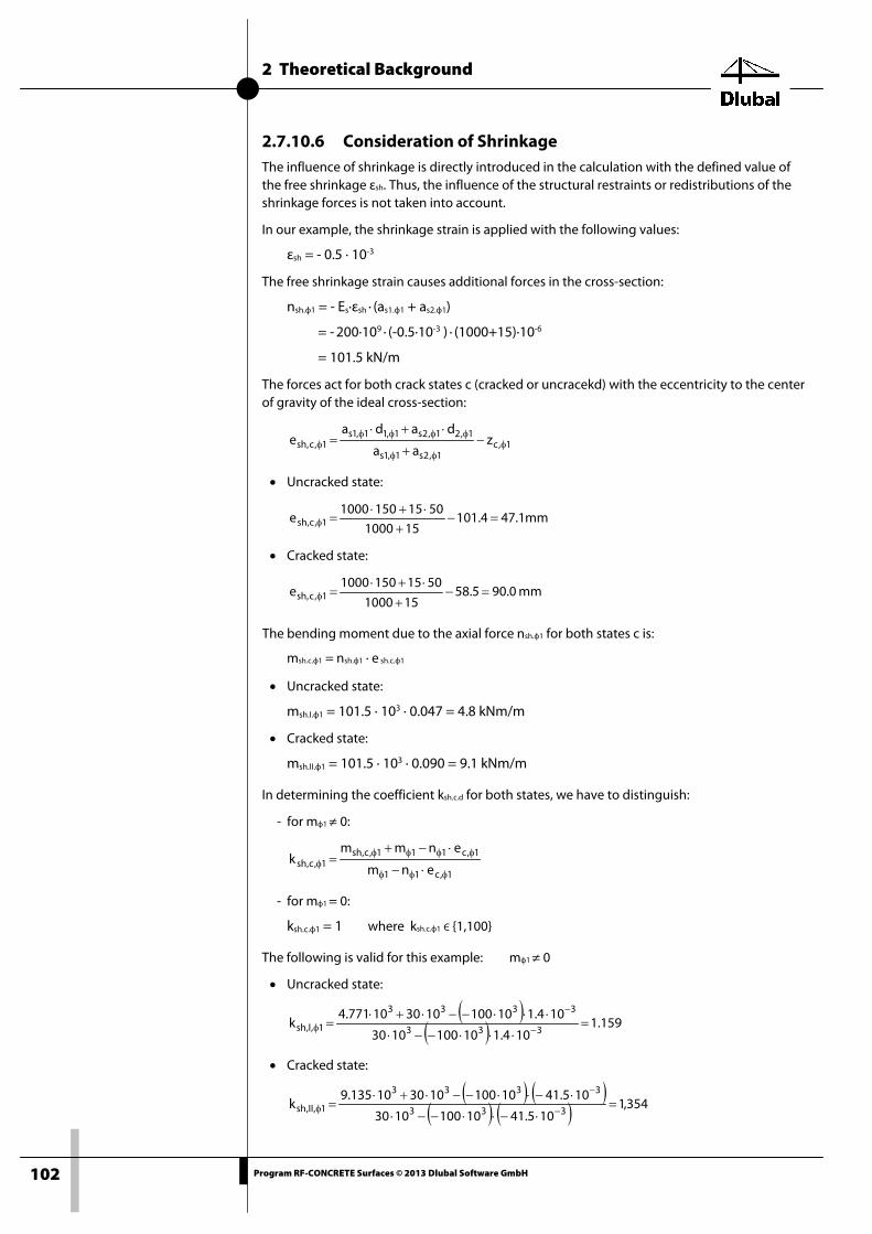
2 Theoretical Background
102 Program RF-CONCRETE Surfaces © 2013 Dlubal Software GmbH
2.7.10.6 Consideration of Shrinkage The influence of shrinkage is directly introduced in the calculation with the defined value of the free shrinkage εsh. Thus, the influence of the structural restraints or redistributions of the shrinkage forces is not taken into account.
In our example, the shrinkage strain is applied with the following values:
εsh = - 0.5 · 10-3
The free shrinkage strain causes additional forces in the cross-section:
nsh.ф1 = - Es·εsh · (as1.ф1 + as2.ф1)
= - 200·109 · (-0.5·10-3 ) · (1000+15)·10-6
= 101.5 kN/m
The forces act for both crack states c (cracked or uncracekd) with the eccentricity to the center of gravity of the ideal cross-section:
1,c1,2s1,1s
1,21,2s1,11,1s1,c,sh z
aa
dadae φ
φφ
φφφφφ −
+
⋅+⋅=
• Uncracked state:
mm1.474.101151000
50151501000e 1,c,sh =−
+⋅+⋅
=φ
• Cracked state:
mm0.905.58151000
50151501000e 1,c,sh =−
+⋅+⋅
=φ
The bending moment due to the axial force nsh.ф1 for both states c is:
msh.c.ф1 = nsh.ф1 · e sh.c.ф1
• Uncracked state:
msh.I.ф1 = 101.5 · 103 · 0.047 = 4.8 kNm/m
• Cracked state:
msh.II.ф1 = 101.5 · 103 · 0.090 = 9.1 kNm/m
In determining the coefficient ksh.c.d for both states, we have to distinguish:
- for mф1 ≠ 0:
1,c11
1,c111,c,sh1,c,sh enm
enmmk
φφφ
φφφφφ ⋅−
⋅−+=
- for mф1 = 0:
ksh.c.ф1 = 1 where ksh.c.ф1 Є 1,100
The following is valid for this example: mф1 ≠ 0
• Uncracked state:
( )( ) 159.1
104.1101001030
104.110100103010771.4k
333
3333
1,I,sh =⋅⋅⋅−−⋅
⋅⋅⋅−−⋅+⋅= −
−
φ
• Cracked state:
( ) ( )( ) ( ) 354,1
105.41101001030
105.4110100103010135.9k
333
3333
1,II,sh =⋅−⋅⋅−−⋅
⋅−⋅⋅−−⋅+⋅= −
−
φ

2 Theoretical Background
103 Program RF-CONCRETE Surfaces © 2013 Dlubal Software GmbH
Figure 2.122: Consideration of shrinkage
2.7.10.7 Calculation of Distribution Coefficient (Damage Parameter) The maximum stress in the uncracked state is:
5,1MPa=
We assume a long-term loading:
βф1 = 0.5
Taking into account Tension Stiffening, the distribution coefficient is calculated according to the following equation:
- for σmax.ф1 > fctm :
2
1max,
ctm1d
f1
σ⋅β−=ζ
φφ
- for σmax.ф1 ≤ fctm :
ζsh.c.ф1 = 0
In the example, the maximum tension stress in concrete is greater than the concrete tension strength.
σmax.ф1 > fctm
5.1 > 2.9
Thus, the distribution coefficient is:
1 1 . 1 . . 11 . 1max, 1 . 1
1. . 1
( )2 ( )
I sh IshI
I I
hm n mn n
hA I
φ φ φ φφ φφ φ
φ φ
χσ χ
− ⋅ − ++= + ⋅ −
3 3 33 3
4
0,20030 10 ( 100 10 ) (0,101 ) 4,778 10100 10 101,5 10 2 (0,200 0,101)
0,206 6,816 10−
⋅ − − ⋅ ⋅ − + ⋅− ⋅ + ⋅= + ⋅ −
⋅
2 21 1
max. 1
2,91 ( ) 1 0,5 ( ) 0,835
5,1ctmf
φ φφ
ζ βσ
= − ⋅ = − ⋅ =

2 Theoretical Background
104 Program RF-CONCRETE Surfaces © 2013 Dlubal Software GmbH
Figure 2.123: Calculation of the distribution coefficient
2.7.10.8 Final Cross-Section Properties The curvature for both states c (cracked / uncracked) is calculated as follows:
• Uncracked state:
• Cracked state:
The strain for both states is determined as follows:
• Uncracked state:
• Cracked state:
Thus, it is possible to determine the mean strain.
εф1 = ζф1 · εII.ф1 + (1 - ζф1) · εI.ф1
= 0.835 · (-10.449 · 10-5) + (1 - 0.835) · (- 4.413 · 10-5) = - 9.459 · 10-5
The mean curvature is determined as follows:
κф1 = ζф1 κф1 κII.ф1 + (1 - ζф1) κI.ф1
= 0.835 · 14.499 · 10-3) + (1 - 0.835) · 4.655 · 10-3 = 12.885 · 10-3
11 . 1, 1 . . 1
. 1
cc sh c
c
m n ek
E Iφφ φ
φ φφ
κ− ⋅
= ⋅⋅
3 3 33
, 1 9 4
30 10 ( 100 10 ) 1, 4 101,158 4,655 10
11 10 6,816 10I φκ
−−
−⋅ − − ⋅ ⋅ ⋅
= ⋅ = ⋅⋅ ⋅ ⋅
3 3 33
, 1 9 4
30 10 ( 100 10 ) ( 41,5 10 )1,353 14, 499 10
11 10 2,193II φκ
−−
−⋅ − − ⋅ ⋅ − ⋅
= ⋅ = ⋅⋅ ⋅
1. 1
. 1c
c
n
E Aφ
φφ
ε =⋅
35
. 1 9
100 104, 413 10
11 10 0,206I φε −− ⋅
= = − ⋅⋅ ⋅
35
. 1 9
100 1010, 449 10
11 10 0,087II φε −− ⋅
= = − ⋅⋅ ⋅

2 Theoretical Background
105 Program RF-CONCRETE Surfaces © 2013 Dlubal Software GmbH
With the mean curvature and the longitudinal strain, it is possible to compute the final cross-section properties taking into account shrinkage, creep, and tension stiffening.
Ideal cross-sectional area
The ideal moment of inertia to the ideal center of the cross-section
218391,50cm=
Eccentricity of centroid
Ideal moment of inertia to the geometric center of cross-section
I0,ф1= Iф1 + Aф1 · e2ф1 = 1.839 · 10-4 + 0.096 · (-0.0393)2 = 33,207.10 cm4
The poisson's ratio is determined as follows:
1,2(1 max ( )) (1 max(0,0.836)) 0.2 0,0328d initdν ς ν∈= − ⋅ = − ⋅ =
Figure 2.124: Final cross-section properties
31 2
1 9 51
100 10958,59
11 10 ( 9, 459 10 )
nA cm
Eφ
φφε −
− ⋅= = =
⋅ ⋅ ⋅ − ⋅
. 1 . 11
1 . 1 . . 1 1 . 1 . . 1(1 )I II
I sh II II sh I
I II
I k I kφ φ
φφ φ φ φ φ φζ ζ
⋅=
⋅ ⋅ + − ⋅ ⋅
4 4
4 4
6,816 10 2,193 10
0,836 6,816 10 1,353 (1 0,836) 2,193 10 1,158
− −
− −⋅ ⋅ ⋅
=⋅ ⋅ ⋅ + − ⋅ ⋅ ⋅
3 3 9 41 1 1
1 31
30 10 12,855 10 11 10 1,839 1039
100 10
m E Ie mm
nφ φ φ
φφ
κ − −− ⋅ ⋅ ⋅ − ⋅ ⋅ ⋅ ⋅ ⋅= = = −
− ⋅
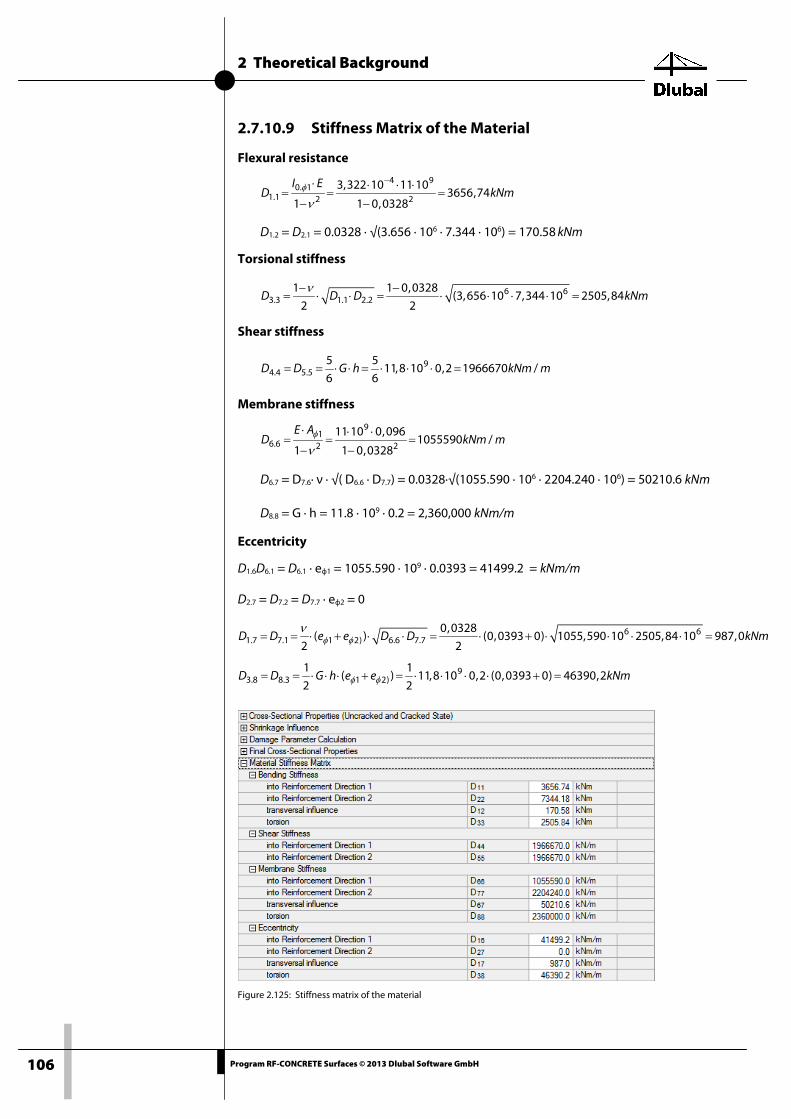
2 Theoretical Background
106 Program RF-CONCRETE Surfaces © 2013 Dlubal Software GmbH
2.7.10.9 Stiffness Matrix of the Material
Flexural resistance
D1.2 = D2.1 = 0.0328 · √(3.656 · 106 · 7.344 · 106) = 170.58 kNm
Torsional stiffness
Shear stiffness
Membrane stiffness
D6.7 = D7.6· ν · √( D6.6 · D7.7) = 0.0328·√(1055.590 · 106 · 2204.240 · 106) = 50210.6 kNm
D8.8 = G · h = 11.8 · 109 · 0.2 = 2,360,000 kNm/m
Eccentricity
D1.6D6.1 = D6.1 · eф1 = 1055.590 · 109 · 0.0393 = 41499.2 = kNm/m
D2.7 = D7.2 = D7.7 · eф2 = 0
Figure 2.125: Stiffness matrix of the material
4 90. 1
1.1 2 2
3,322 10 11 103656,74
1 1 0,0328
I ED kNmφ
ν
−⋅ ⋅ ⋅ ⋅= = =
− −
6 63.3 1.1 2.2
1 1 0,0328(3,656 10 7,344 10 2505,84
2 2D D D kNm
ν− −= ⋅ ⋅ = ⋅ ⋅ ⋅ ⋅ =
94.4 5.5
5 511,8 10 0,2 1966670 /
6 6D D G h kNm m= = ⋅ ⋅ = ⋅ ⋅ ⋅ =
91
6.6 2 2
11 10 0,0961055590 /
1 1 0,0328
E AD kNm mφ
ν
⋅ ⋅ ⋅= = =
− −
6 61.7 7.1 1 2) 6.6 7.7
0,0328( ) (0,0393 0) 1055,590 10 2505,84 10 987,0
2 2D D e e D D kNmφ φ
ν= = ⋅ + ⋅ ⋅ = ⋅ + ⋅ ⋅ ⋅ ⋅ =
93.8 8.3 1 2)
1 1( ) 11,8 10 0,2 (0,0393 0) 46390,2
2 2D D G h e e kNmφ φ= = ⋅ ⋅ ⋅ + = ⋅ ⋅ ⋅ ⋅ + =

2 Theoretical Background
107 Program RF-CONCRETE Surfaces © 2013 Dlubal Software GmbH
2.8 Nonlinear Method 2.8.1 General
The serviceability limit state (SLS) design is generally divided the three following groups:
• Stress limitation (EN 1992-1-1, clause 7.2)
• Crack control (EN 1992-1-1, clause 7.3)
• Deflection control (EN 1992-1-1, clause 7.4)
The design of concrete structures is usually based on linear structural analyses: To determine the reinforcement, including the serviceability limit state design, the internal forces are deter-mined linearly; the cross-section analysis is performed subsequently. However, this procedure takes into account the cracking typical for reinforced concrete with the corresponding nonlin-ear material rules of reinforced concrete only on the cross-section level.
By including the nonlinear behavior of reinforced concrete in the determination of internal forces, we obtain realistic states of stress and, therefore, distributions of internal forces that in statically indeterminate systems differ significantly – due to stiffness redistributions – from the linearly determined internal forces,. For the serviceability limit state design, this means that we must take into account the nonlinear material behavior of reinforced concrete to obtain a real-istic calculation of deformations, stresses, and crack widths.
If the cracking is not taken into account in the deformation calculation, the occurring defor-mations will be underestimated. By considering creeping and shrinkage, the deformation may be 3 to 8 times larger, depending on the stress and boundary conditions. The add-on module RF-CONCRETE NL allows for the realistic calculation of the deformations, crack widths, and stresses of reinforced concrete surfaces by considering the nonlinear material behavior in the determination of internal forces.
2.8.2 Equations and Methods of Approximations
2.8.2.1 Theoretical Approaches
"Nonlinear calculation" refers to the determination of internal forces and deformations taking into account the nonlinear behavior of internal forces and deformations (physical).
Surface models can be described as two-dimensional structures with the following functions of state: surface loads, deformations, internal forces, and strains in the centroids of the surface areas. However, material properties that vary over the depth of the area must be taken into ac-count for the nonlinear reinforced concrete model. Hence, it becomes necessary to extend the 2D model by additionally taking into account the depth of the cross-section. The cross-section of the reinforced concrete is subdivided into a number of reinforcing steel and concrete layers (see Figure 2.126).
Based on the strains in the centroids of the areas, under the assumption of the Bernoulli hy-pothesis, we obtain the strains for each layer. After applying the corresponding reinforcing steel and concrete laws to the strains, we obtain the stresses. The resulting stresses per layer can be integrated into internal forces of the total cross-section.

2 Theoretical Background
108 Program RF-CONCRETE Surfaces © 2013 Dlubal Software GmbH
Figure 2.126: Layer model for reinforced concrete surfaces
If the tension strength of concrete is reached in a point of the structure, a discontinuity occurs in the form of a crack. If taken strictly, this would require an adjustment of the discretization (remeshing) to include every crack in the calculation in its actual position and extension. For several cracks, this method would result in a high numerical effort, because every crack would increase the number of elements. Therefore, occurring cracks are "smeared" within an element and the stiffness-reducing influences of the cracks are taken into account by adjusting the ma-terial rule in the calculation.
If the first principal stress in a concrete layer reaches the concrete tensile strength, a crack is formed perpendicular to the first principal direction of stress. This principal direction can change if the load changes. Here we can assume that a forming crack does not change its posi-tion and orientation (the so-called fixed crack model) or that the crack always runs orthogonally to the variable principal direction (rotating crack model). RF-CONCRETE NL uses the rotating crack model.
Figure 2.127: Crack models in reinforced concrete surface elements

2 Theoretical Background
109 Program RF-CONCRETE Surfaces © 2013 Dlubal Software GmbH
No
2.8.2.2 Flowchart
Figure 2.128: Flowchart
where eD Stiffness matrix of the material, constitutive matrix
B Matrix due to the geometry and the basic type of the FE function ee dB ⋅=ε
eMK Material FE stiffness matrix eK σ Geometric FE stiffness matrix eTK FE overall stiffness matrix gK Global stiffness matrix of the entire model
eD
Import model data
FE stiffness matrix e T eM d
Ω
= Ω∫K B D B
Overall stiffness matrix as sum of the material and geometric FE stiffness matrix of the element e e e
T M σ= +K K K
Stiffness matrix of the material eD for the first iteration step E, µ, G, h ⇒
eD
Global stiffness matrix as sum of the extended FE stiffness matrices g e
Te
= ∑K K
Global vector of the nodal forces (loading) as sum of the extended vectors of the FE nodal forces of the element g e
e= ∑f f
Solving the equation system g g g⋅ =K d f to determine the global vector
of the nodal parameters of the deformations gd
Nodal parameters of the FE deformations by separation from the global vector of the nodal parameters of the deformation g e
e= ∑d d
Strain vector e e= ⋅ε B d
Internal forces e e e= ⋅σ D ε are always in equilibrium in an unconverged
calculation, but not in the stress-strain diagram
Material nonlinear calculation with generation of new stiffness matrix
of the material eD due to strain vector
eε and stress-strain diagram
Result: Internal forces eσ that are not in equilibrium in the unconverged
calculation, but always correspond to the stress-strain diagram
Display results
Yes Yes No
Are the conver-gence criteria met?
Is max number of iterations reached?
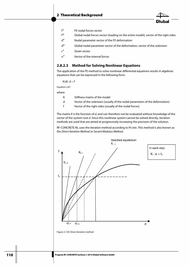
2 Theoretical Background
110 Program RF-CONCRETE Surfaces © 2013 Dlubal Software GmbH
ef FE nodal forces vector gf Global nodal forces vector (loading on the entire model), vector of the right sides ed Nodal parameter vector of the FE deformation gd Global nodal parameter vector of the deformation, vector of the unknown eε Strain vector eσ Vector of the internal forces
2.8.2.3 Method for Solving Nonlinear Equations The application of the FE method to solve nonlinear differential equations results in algebraic equations that can be expressed in the following form:
fd)d(K =⋅
Equation 2.87
where
K Stiffness matrix of the model
d Vector of the unknown (usually of the nodal parameters of the deformation)
f Vector of the right sides (usually of the nodal forces)
The matrix K is the function of d, and can therefore not be evaluated without knowledge of the vector of the system root d. Since this nonlinear system cannot be solved directly, iteration methods are used that are aimed at progressively increasing the precision of the solution.
RF-CONCRETE NL uses the iteration method according to PICARD. This method is also known as the Direct Iteration Method or Secant Modulus Method.
Figure 2.129: Direct iteration method

2 Theoretical Background
111 Program RF-CONCRETE Surfaces © 2013 Dlubal Software GmbH
2.8.2.4 Convergence Criteria In solving the nonlinear equations, two convergence criteria are considered. The iteration step is deemed to be completed when one convergence criterion is satisfied. The first convergence criterion observes how the diagonal components of the stiffness matrix of the material change. A convergence is reached when the stiffness matrix of the material has stabilized for all finite elements.
=−
−
−
1in
1ij
1itot
D
...
D
D
=in
ij
itot
D
...
D
D ε≤
−
∑
∑
=
−
=
−
n
1j
1ij
n
1j
1ij
ij
D
DD
Equation 2.88
where 1i
totD − Stiffness matrix of the material from the previous iteration step.
itotD Stiffness matrix of the material in the current iteration step
ε Desired precision (for RFEM precision, the following applies 1: ε = 0.05 %)
The second convergence criterion observes how the size of the maximum deformation chang-es. At the same time, the program controls whether the place of the maximum deformation within the structure has changed. Since the deformation usually converges faster than the stiffness matrix, the deformation criterion is activated only after 50 iteration steps (for RFEM precision 1).
ε<−−
−
1imax
1imax
imax
d
dd and 1i
maximax NN −=
Equation 2.89
where 1i
maxd − Maximum nodal displacement from the previous iteration step
imaxd Maximum nodal displacement of the structure in the current iteration step
ε Desired precision (for RFEM precision 1, the following applies: ε = 0.05 %)
1imaxN − Number of the node with maximum displacement from previous iteration step
imaxN Number of the node with maximum displacement from current iteration step
The precision of the convergence criterion for the nonlinear calculation and the point in time defining after which iteration step the deformation criterion is additionally considered are con-trolled in the Global Calculation Parameters tab of the Calculation Parameters dialog box in RFEM. You can also open this dialog box in the 1.1 General Data window of RF-CONCRETE Surfaces:
Figure 2.130: [Edit Settings] button in the Serviceability Limit State tab of the 1.1 General Data window
The Settings for Nonlinear Calculation appears (see the following figure).

2 Theoretical Background
112 Program RF-CONCRETE Surfaces © 2013 Dlubal Software GmbH
Then we click [Details] to open the RFEM dialog box Calculation Parameters.
Figure 2.131: Dialog box Settings for Nonlinear Calculation with access to the convergence criterion of RFEM
The value for the Precision of convergence criteria ("RFEM precision") in the RFEM dialog box in-fluences the break-off limit ε for the physically nonlinear calculation and the iteration step ni from which on the deformation criterion is additionally considered:
ε = "RFEM precision" · 0.05 % ni = 1/"RFEM precision" · 50
The default value of the RFEM precision is 1. Thus, the precision of the convergence criterion for the physical nonlinearity is ε = 0.05 % and the additional consideration of the deformation criterion starts after the 50th iteration step. For a higher precision, it is necessary to reduce the value of the RFEM precision. Thus, ε becomes smaller and the deformation criterion is consid-ered later.

2 Theoretical Background
113 Program RF-CONCRETE Surfaces © 2013 Dlubal Software GmbH
2.8.3 Material Properties
2.8.3.1 Concrete in Compression
In the serviceability limit state design, the mean strengths of the materials are used for the cal-culation. In the compressed area, it is possible to choose between a parabola and a parabola-rectangle distribution of the stress-strain relationship.
Figure 2.132: Stress-strain diagram for concrete in compression
The relevant settings are specified in the Material Properties tab of the Settings for Nonlinear Calculation dialog box (see Figure 3.11, page 135). You can open the dialog box in the Service-ability Limit State tab of the 1.1 General Data window by clicking the button shown on the left (see Figure 2.130).
2.8.3.2 Concrete in Tension
There are several options for the stress-strain relationship of the concrete in tension.
Figure 2.133: Stress-strain diagram for concrete in tension

2 Theoretical Background
114 Program RF-CONCRETE Surfaces © 2013 Dlubal Software GmbH
The tensile strength of the concrete can, for example, be considered according to the specifi-cations of the CEB-FIP Model Code 90:1993. Until the tensile strength of concrete fctm is reached, the program assumes the distribution shown in Figure 2.134 to reach the crack strain of 0.15 ‰.
Figure 2.134: Stress-strain relationship for concrete in tension according to CEB-FIP Model Code 90:1993
Alternatively, you can use tension stiffening. This procedure is described in the following chapter.
Figure 2.135: Stress-strain diagram for tension stiffening
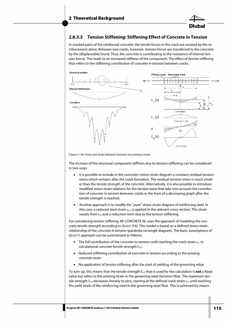
2 Theoretical Background
115 Program RF-CONCRETE Surfaces © 2013 Dlubal Software GmbH
2.8.3.3 Tension Stiffening: Stiffening Effect of Concrete in Tension
In cracked parts of the reinforced concrete, the tensile forces in the crack are resisted by the re-inforcement alone. Between two cracks, however, tension forces are transferred to the concrete by the (displaceable) bond. Thus, the concrete is contributing to the resistance of internal ten-sion forces. This leads to an increased stiffness of the component. The effect of tension stiffening thus refers to the stiffening contribution of concrete in tension between cracks.
Figure 2.136: Stress and strain behavior between two primary cracks
The increase of the structural component stiffness due to tension stiffening can be considered in two ways:
• It is possible to include in the concrete's stress-strain diagram a constant residual tension stress which remains after the crack formation. The residual tension stress is much small-er than the tensile strength of the concrete. Alternatively, it is also possible to introduce modified stress-strain relations for the tension zone that take into account the contribu-tion of concrete in tension between cracks in the form of a decreasing graph after the tensile strength is reached.
• Another approach is to modify the "pure" stress-strain diagram of reinforcing steel. In this case, a reduced steel strain εsm is applied in the relevant cross-section. This strain results from εs2 and a reduction term due to the tension stiffening.
For considering tension stiffening, RF-CONCRETE NL uses the approach of modeling the con-crete tensile strength according to QUAST [16]. This model is based on a defined stress-strain relationship of the concrete in tension (parabola-rectangle diagram). The basic assumptions of QUAST's approach can be summarized as follows:
• The full contribution of the concrete to tension until reaching the crack strain εcr or calculational concrete tensile strength fct,R
• Reduced stiffening contribution of concrete in tension according to the existing concrete strain
• No application of tension stiffening after the start of yielding of the governing rebar
To sum up, this means that the tensile strength fct,R that is used for the calculation is not a fixed value but refers to the existing strain in the governing steel (tension) fiber. The maximum ten-sile strength fct,R decreases linearly to zero, starting at the defined crack strain εcr until reaching the yield strain of the reinforcing steel in the governing steel fiber. This is achieved by means
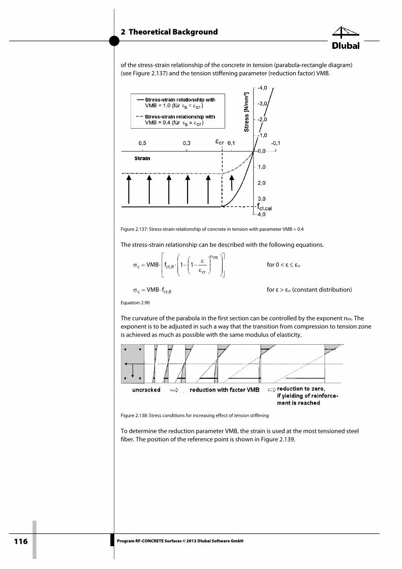
2 Theoretical Background
116 Program RF-CONCRETE Surfaces © 2013 Dlubal Software GmbH
of the stress-strain relationship of the concrete in tension (parabola-rectangle diagram) (see Figure 2.137) and the tension stiffening parameter (reduction factor) VMB.
Figure 2.137: Stress-strain relationship of concrete in tension with parameter VMB = 0.4
The stress-strain relationship can be described with the following equations.
εε
−−⋅⋅=σPRn
crR,ctc 11fVMB for 0 < ε ≤ εcr
R,ctc fVMB ⋅=σ for ε > εcr (constant distribution)
Equation 2.90
The curvature of the parabola in the first section can be controlled by the exponent nPR. The exponent is to be adjusted in such a way that the transition from compression to tension zone is achieved as much as possible with the same modulus of elasticity.
Figure 2.138: Stress conditions for increasing effect of tension stiffening
To determine the reduction parameter VMB, the strain is used at the most tensioned steel fiber. The position of the reference point is shown in Figure 2.139.

2 Theoretical Background
117 Program RF-CONCRETE Surfaces © 2013 Dlubal Software GmbH
Figure 2.139: Determination of residual tensile strength for Tension Stiffening according to QUAST [16]
The reduction parameter VMB decreases with increasing steel strain. In the diagram for param-eter VMB (see Figure 2.140), we can see that the parameter VMB is reduced to zero exactly at the point when the yielding of the reinforcement starts.
Figure 2.140: Reduction parameter VMB
The distribution for the reduction parameter VMB in state II (ε > εcr ) can be controlled by means of the exponent nVMB. The experiential values according to PFEIFFER [11] are the values nVMB = 1(linear) to nVMB =2 (parabola) for bending elements. QUAST [17] uses the exponent nVMB = 1(linear), thus achieving a good match for the check calculation of column tests. According to PFEIFFER [11], it is possible to represent pure tension tests showing acceptable matches by using nVMB = 2.

2 Theoretical Background
118 Program RF-CONCRETE Surfaces © 2013 Dlubal Software GmbH
The assumption of a parabola-rectangle diagram for a cracked tension zone of concrete can be regarded as a computational aid. At first glance, there are great differences compared to the experimentally determined stress-strain diagrams on the tension face of the pure concrete.
Figure 2.141: Comparison of model and laboratory test
The given stresses in the reinforced concrete cross-section in bending show that the parabola-rectangle diagram is indeed better suited to describe the mean of the strains and stresses.
In a bending beam, a concrete body forms between the cracks. It acts as a kind of wall, into which tension forces are reintroduced gradually by the reinforcement. This results in a very ir-regular distribution of stress and strain. For the mean, however, we can create a plane of strain with a parabola-rectangle distribution with which it is possible to consider the mean curvature.
Figure 2.142: Existing state of stress when subjected to bending
QUAST suggests the following calculation value for the tension strength fct,R and the crack strain ecr,R for his model.
cmR,ct f201
f ⋅= 1cR,cr 201
ε⋅=ε
Equation 2.91
The calculational value for the tension strength fct,R is thus smaller than specified by the Euro-codes. This is due to the description of the stress-strain relation and the determination of the reduction parameter VMB, where the assumed tension stress and the resulting tension force after the exceeding of the tension strain are reduced only slowly. For a strain of 2·εcr, there is al-so an acting tension stress of about 0.95·fct,R. Thus, in case of bending, the reduction of the stiff-ness can be well predicted. In case of pure tension, the values for fct,R are too low. According to PFEIFFER [11], the values from EC2 should be taken for the calculation value of the tension strength.

2 Theoretical Background
119 Program RF-CONCRETE Surfaces © 2013 Dlubal Software GmbH
The values recommended by QUAST [17] for fct,R = 1/20 · fcm can be obtained by taking 60 % of the tensile strengths given in EC2. On the one hand, the cracking of the cross-section is pre-dicted too early when applying fct,R = 0.6 · fctm. On the other hand, this already takes into ac-count a reduction of the tensile strength under permanent load (ca. 70 %) or a temporarily higher load (for example, the short-term application of the rare combination of action) that results in a damaged tension zone.
The individual calculation values for the tensile zone of the concrete can be described as fol-lows:
dardtans,ctR,ct f60,0f ⋅= Calculational tensile strength
dardtans,ct
cm
f
f=ν Ratio, auxiliary value
νε
=ε 1cR,cr Calculational crack strain
cm
1ccmPR f
E1.1nε
⋅⋅= Exponent for general parabola (for Equation 2.90)
Equation 2.92
2.8.3.4 Reinforcing Steel For the serviceability limit state design, the mean strengths of the materials are used in the calculation. The mean reinforcing steel strengths were published by the JCSS in Probabilistic Model Code. This code specifies the mean value of the yield strength with fym = 1.1 · fyk.
RF-CONCRETE NL uses a bilinear distribution for the stress-strain relationship of reinforcing steel.
Figure 2.143: Stress-strain relationship of reinforcing steel
You can choose if the graph of plasticity is horizontal or increases up to ftm. The settings are specified in the Settings for Nonlinear Calculation dialog box (see Figure 3.11, page 135). To open this dialog box, click the button shown on the left that can be found in the Serviceability Limit State tab of the 1.1 General Data window.
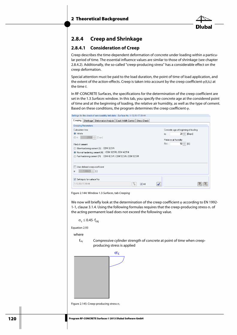
2 Theoretical Background
120 Program RF-CONCRETE Surfaces © 2013 Dlubal Software GmbH
2.8.4 Creep and Shrinkage
2.8.4.1 Consideration of Creep Creep describes the time-dependent deformation of concrete under loading within a particu-lar period of time. The essential influence values are similar to those of shrinkage (see chapter 2.8.4.2). Additionally, the so-called "creep-producing stress" has a considerable effect on the creep deformation.
Special attention must be paid to the load duration, the point of time of load application, and the extent of the action-effects. Creep is taken into account by the creep coefficient ϕ(t,t0) at the time t.
In RF-CONCRETE Surfaces, the specifications for the determination of the creep coefficient are set in the 1.3 Surfaces window. In this tab, you specify the concrete age at the considered point of time and at the beginning of loading, the relative air humidity, as well as the type of cement. Based on these conditions, the program determines the creep coefficient ϕ.
Figure 2.144: Window 1.3 Surfaces, tab Creeping
We now will briefly look at the determination of the creep coefficient ϕ according to EN 1992-1-1, clause 3.1.4. Using the following formulas requires that the creep-producing stress σc of the acting permanent load does not exceed the following value.
ckjc f45.0 ⋅≤σ
Equation 2.93
where
fckj Compressive cylinder strength of concrete at point of time when creep-producing stress is applied
Figure 2.145: Creep-producing stress σc
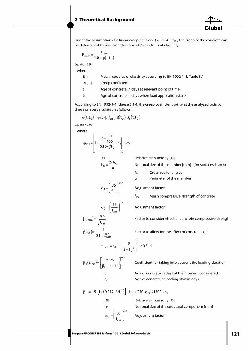
2 Theoretical Background
121 Program RF-CONCRETE Surfaces © 2013 Dlubal Software GmbH
Under the assumption of a linear creep behavior (σc < 0.45 · fckj), the creep of the concrete can be determined by reducing the concrete's modulus of elasticity.
( )0
cmeff,c t,t0.1
EE
ϕ+=
Equation 2.94
where
Ecm Mean modulus of elasticity according to EN 1992-1-1, Table 3.1
ϕ(t,t0) Creep coefficient
t Age of concrete in days at relevant point of time
t0 Age of concrete in days when load application starts
According to EN 1992-1-1, clause 3.1.4, the creep coefficient ϕ(t,t0) at the analyzed point of time t can be calculated as follows.
( ) ( ) ( ) ( )0c0cmRH0 t,ttft,t β⋅β⋅β⋅ϕ=ϕ
Equation 2.95
where
2130
RHh10.0
100RH
11 α⋅
α⋅⋅
−+=ϕ
RH Relative air humidity [%]
u
A2h c
0⋅
= Notional size of the member [mm] (for surfaces: h0 = h)
Ac Cross-sectional area
u Perimeter of the member
7.0
cm1 f
35
=α Adjustment factor
fcm Mean compressive strength of concrete
2.0
cm2 f
35
=α Adjustment factor
( )cm
cmf
8.16f =β Factor to consider effect of concrete compressive strength
( )2.0eff,0
0t1.0
1t
+=β Factor to allow for the effect of concrete age
d5.0t2
91tt
2.10
0eff,o ⋅≥
++=
α
( )3,0
0H
00c tt
ttt,t
−+β
−=β Coefficient for taking into account the loading duration
t Age of concrete in days at the moment considered
t0 Age of concrete at loading start in days
( )[ ] 33018
H 1500250hRH012.015.1 α⋅≤α⋅+⋅⋅+⋅=β
RH Relative air humidity [%]
h0 Notional size of the structural component [mm]
5.0
cm3 f
35
=α Adjustment factor
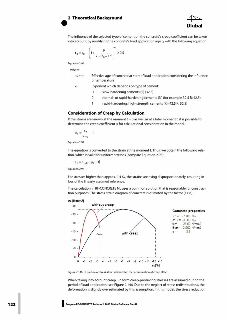
2 Theoretical Background
122 Program RF-CONCRETE Surfaces © 2013 Dlubal Software GmbH
The influence of the selected type of cement on the concrete's creep coefficient can be taken into account by modifying the concrete's load application age t0 with the following equation:
( ) 5.0t2
91tt
2.1T,0
T,00 ≥
++⋅=
α
Equation 2.96
where
t0 = tT Effective age of concrete at start of load application considering the influence of temperature
α Exponent which depends on type of cement:
-1 slow-hardening cements (S) (32.5)
0 normal- or rapid-hardening cements (N) (for example 32.5 R; 42.5)
1 rapid-hardening, high-strength cements (R) (42.5 R; 52.5)
Consideration of Creep by Calculation If the strains are known at the moment t = 0 as well as at a later moment t, it is possible to determine the creep coefficient ϕ for calculational consideration in the model.
10t
tt −
εε
=ϕ=
Equation 2.97
The equation is converted to the strain at the moment t. Thus, we obtain the following rela-tion, which is valid for uniform stresses (compare Equation 2.93):
( )1t0tt +ϕ⋅ε=ε =
Equation 2.98
For stresses higher than approx. 0.4 fck, the strains are rising disproportionately, resulting in loss of the linearly assumed reference.
The calculation in RF-CONCRETE NL uses a common solution that is reasonable for construc-tion purposes. The stress-strain diagram of concrete is distorted by the factor (1+ ϕ).
Figure 2.146: Distortion of stress-strain relationship for determination of creep effect
When taking into account creep, uniform creep-producing stresses are assumed during the period of load application (see Figure 2.146. Due to the neglect of stress redistributions, the deformation is slightly overestimated by this assumption. In this model, the stress reduction
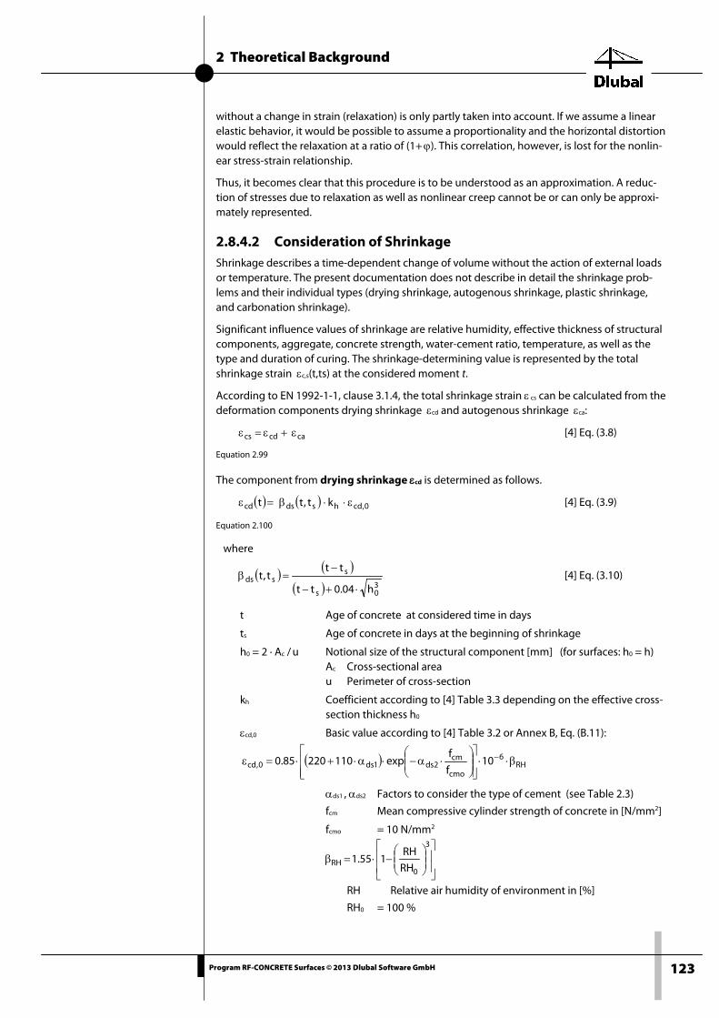
2 Theoretical Background
123 Program RF-CONCRETE Surfaces © 2013 Dlubal Software GmbH
without a change in strain (relaxation) is only partly taken into account. If we assume a linear elastic behavior, it would be possible to assume a proportionality and the horizontal distortion would reflect the relaxation at a ratio of (1+ ϕ). This correlation, however, is lost for the nonlin-ear stress-strain relationship.
Thus, it becomes clear that this procedure is to be understood as an approximation. A reduc-tion of stresses due to relaxation as well as nonlinear creep cannot be or can only be approxi-mately represented.
2.8.4.2 Consideration of Shrinkage Shrinkage describes a time-dependent change of volume without the action of external loads or temperature. The present documentation does not describe in detail the shrinkage prob-lems and their individual types (drying shrinkage, autogenous shrinkage, plastic shrinkage, and carbonation shrinkage).
Significant influence values of shrinkage are relative humidity, effective thickness of structural components, aggregate, concrete strength, water-cement ratio, temperature, as well as the type and duration of curing. The shrinkage-determining value is represented by the total shrinkage strain εc,s(t,ts) at the considered moment t.
According to EN 1992-1-1, clause 3.1.4, the total shrinkage strain ε cs can be calculated from the deformation components drying shrinkage εcd and autogenous shrinkage εca:
cacdcs ε+ε=ε [4] Eq. (3.8)
Equation 2.99
The component from drying shrinkage εcd is determined as follows.
( ) ( ) 0,cdhsdscd kt,tt ε⋅⋅β=ε [4] Eq. (3.9)
Equation 2.100
where
( ) ( )( ) 3
0s
ssds
h04.0tt
ttt,t
⋅+−
−=β
[4] Eq. (3.10)
t Age of concrete at considered time in days
ts Age of concrete in days at the beginning of shrinkage
h0 = 2 · Ac / u Notional size of the structural component [mm] (for surfaces: h0 = h) Ac Cross-sectional area u Perimeter of cross-section
kh Coefficient according to [4] Table 3.3 depending on the effective cross- section thickness h0
εcd,0 Basic value according to [4] Table 3.2 or Annex B, Eq. (B.11):
( ) RH6
cmo
cm2ds1ds0,cd 10
f
fexp11022085.0 β⋅⋅
⋅α−⋅α⋅+⋅=ε −
αds1 , αds2 Factors to consider the type of cement (see Table 2.3)
fcm Mean compressive cylinder strength of concrete in [N/mm2]
fcmo = 10 N/mm2
−⋅=β
3
0RH RH
RH155.1
RH Relative air humidity of environment in [%]
RH0 = 100 %

2 Theoretical Background
124 Program RF-CONCRETE Surfaces © 2013 Dlubal Software GmbH
Cement Class Characteristic αds1 αds2
32.5 N S Slow-hardening 3 0.13
32.5 R; 42.5 R N Normal- or rapid-hardening 4 0.12
42.5 R; 52.5 N/R R Rapid-hardening 6 0.11
Table 2.3: Coefficients αas, αds1, αds2 depending on the type of cement
The autogenous shrinkage strain εca is determined as follows.
( ) ( ) ( )∞ε⋅β=ε caasca tt
[4] Eq. (3.11)
Equation 2.101
where
( ) t2.0as e1t −−=β
[4] Eq. (3.12)
( ) ( ) 6
ckca 1010f5.2 −⋅−⋅=∞ε
[4] Eq. (3.13)
t in days
Consideration of shrinkage in RF-CONCRETE NL (with consideration of the reinforcement) The data for the determination of shrinkage strain is entered in the 1.3 Surfaces window. There, you specify the age of concrete at the considered moment and at the beginning of shrinkage, the relative air humidity, and the type of cement. Based on these specifications, RF-CONCRETE NL determines the shrinkage ε.
Figure 2.147: Window 1.3 Surfaces, tab Shrinkage
The shrinkage strain εc,s(t,ts) can also be specified manually and independent of standards.
The shrinkage strain is only applied to the concrete layers; the reinforcement layers are not considered. Thus, there is a difference to the classical temperature loading, which also affects the reinforcement layers. The model for shrinkage used in RF-CONCRETE NL thus considers the restraint of the shrinkage strain εsh that is exerted by the reinforcement or the cross-section curvature of an unsymmetrical reinforcement. The resulting loads from the shrinkage strain are automatically applied as virtual loads to the surfaces, and calculated. Depending on the struc-tural system, the shrinkage strain results in additional stresses (statically indeterminate system) or deformations (statically determinate system). For shrinkage, RF-CONCRETE NL takes into ac-count the influence of the structural boundary conditions in different ways.
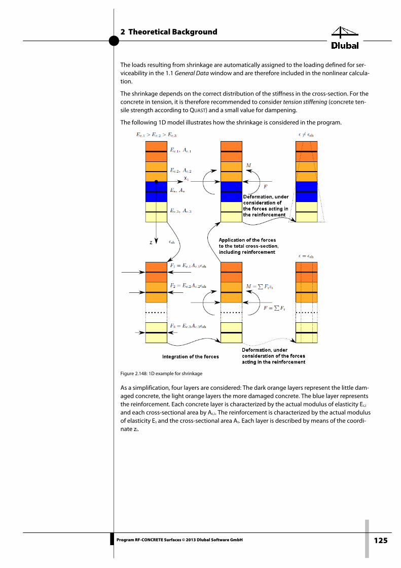
2 Theoretical Background
125 Program RF-CONCRETE Surfaces © 2013 Dlubal Software GmbH
The loads resulting from shrinkage are automatically assigned to the loading defined for ser-viceability in the 1.1 General Data window and are therefore included in the nonlinear calcula-tion.
The shrinkage depends on the correct distribution of the stiffness in the cross-section. For the concrete in tension, it is therefore recommended to consider tension stiffening (concrete ten-sile strength according to QUAST) and a small value for dampening.
The following 1D model illustrates how the shrinkage is considered in the program.
Figure 2.148: 1D example for shrinkage
As a simplification, four layers are considered: The dark orange layers represent the little dam-aged concrete, the light orange layers the more damaged concrete. The blue layer represents the reinforcement. Each concrete layer is characterized by the actual modulus of elasticity Ec,i and each cross-sectional area by Ac,i. The reinforcement is characterized by the actual modulus of elasticity Es and the cross-sectional area As. Each layer is described by means of the coordi-nate zi.

2 Theoretical Background
126 Program RF-CONCRETE Surfaces © 2013 Dlubal Software GmbH
Consideration of Shrinkage as External Load The shrinkage strain can also be applied in RFEM as external load. In the New Surface Load dia-log box of RFEM, you can open the Generate Surface Load Due to Shrinkage dialog box by click-ing the button shown on the left.
Figure 2.149: RFEM dialog box Generate Surface Load Due to Shrinkage
In this dialog box, you can enter the parameters to determine the shrinkage strain. By clicking [OK], you transfer the determined shrinkage as load magnitude to the initial dialog box New Surface Load. The load type is automatically set to Axial strain. Please note that the shrinkage strain acts on the entire cross-section, and that possible restraints or cross-section curvatures are not taken into account by the reinforcement.
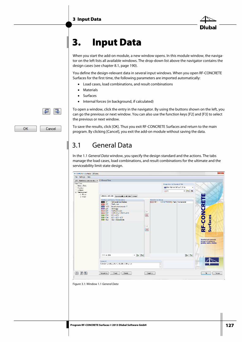
3 Input Data
127 Program RF-CONCRETE Surfaces © 2013 Dlubal Software GmbH
3. Input Data When you start the add-on module, a new window opens. In this module window, the naviga-tor on the left lists all available windows. The drop-down list above the navigator contains the design cases (see chapter 8.1, page 190).
You define the design-relevant data in several input windows. When you open RF-CONCRETE Surfaces for the first time, the following parameters are imported automatically:
• Load cases, load combinations, and result combinations
• Materials
• Surfaces
• Internal forces (in background, if calculated)
To open a window, click the entry in the navigator. By using the buttons shown on the left, you can go the previous or next window. You can also use the function keys [F2] and [F3] to select the previous or next window.
To save the results, click [OK]. Thus you exit RF-CONCRETE Surfaces and return to the main program. By clicking [Cancel], you exit the add-on module without saving the data.
3.1 General Data In the 1.1 General Data window, you specify the design standard and the actions. The tabs manage the load cases, load combinations, and result combinations for the ultimate and the serviceability limit state design.
Figure 3.1: Window 1.1 General Data

3 Input Data
128 Program RF-CONCRETE Surfaces © 2013 Dlubal Software GmbH
Design Acc. to Standard / NA
Figure 3.2: Standard and National Annex for reinforced concrete design
Standard
Specify the standard for the serviceability limit state design and the ultimate limit state design. The following standards for reinforced concrete can be selected from the list:
• EN 1992-1-1:2004/AC:2010 European Union
• DIN 1045-1:2008-08 Germany
• DIN 1045:1988-07 Germany
• ACI 318-11 United States of America
• SIA 262:2003 Switzerland
• GB 50010-2010 China
You can purchase each standard separately.
National Annex
For the design according to Eurocode (EN 1992-1-1:2004/AC:2010), you have to specify the National Annex whose parameters apply for the checks.
Figure 3.3: National Annexes for EN 1992-1-1
Click [Edit] to view the preset values.
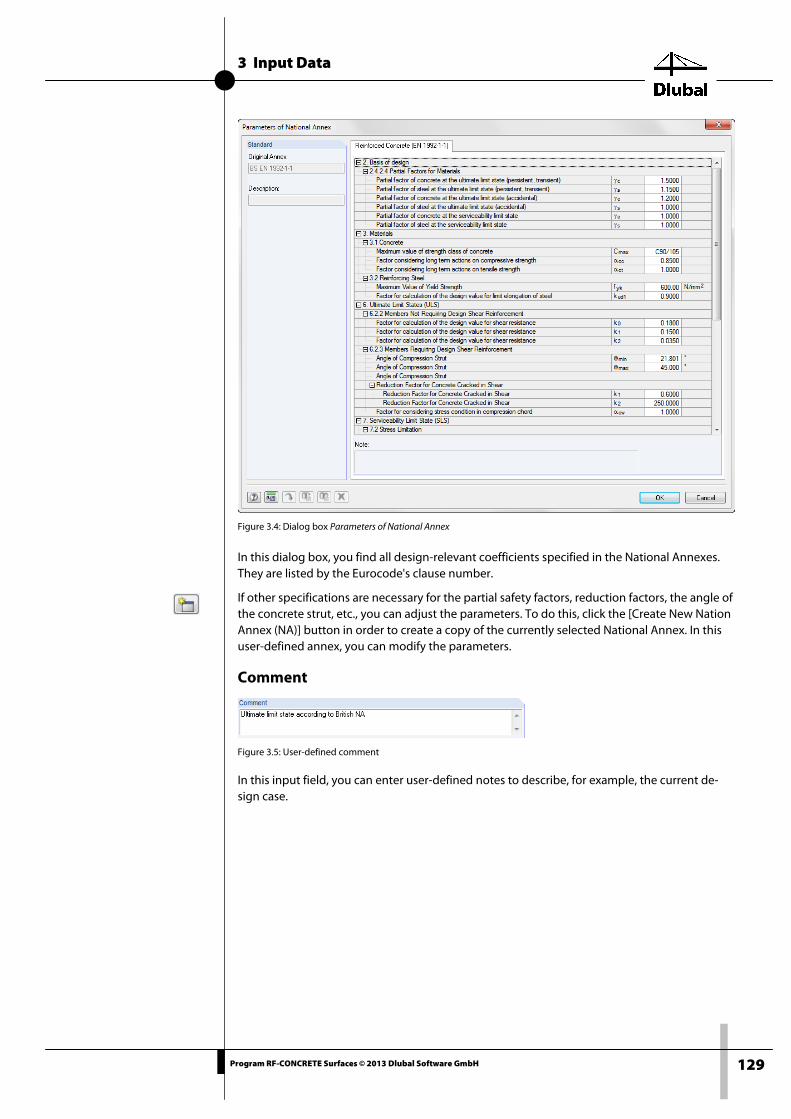
3 Input Data
129 Program RF-CONCRETE Surfaces © 2013 Dlubal Software GmbH
Figure 3.4: Dialog box Parameters of National Annex
In this dialog box, you find all design-relevant coefficients specified in the National Annexes. They are listed by the Eurocode's clause number.
If other specifications are necessary for the partial safety factors, reduction factors, the angle of the concrete strut, etc., you can adjust the parameters. To do this, click the [Create New Nation Annex (NA)] button in order to create a copy of the currently selected National Annex. In this user-defined annex, you can modify the parameters.
Comment
Figure 3.5: User-defined comment
In this input field, you can enter user-defined notes to describe, for example, the current de-sign case.

3 Input Data
130 Program RF-CONCRETE Surfaces © 2013 Dlubal Software GmbH
3.1.1 Ultimate Limit State
Figure 3.6: Window 1.1 General Data, tab Ultimate Limit State
Existing Load Cases / Combinations This column lists all load cases, load combinations, and result combinations created in RFEM.
Click [] to transfer the selected entries to the list Selected for Design on the right. You can also double-click the items to select them for design. To transfer the complete list to the right, click [].
To select several load cases at the same time, click them one by one while pressing [Ctrl]. This allows you to transfer several load cases at once.
If a load case is marked by an asterisk (*), like LC3 in Figure 3.6, it is not possible to calculate it: It indicates a load case without load data or a load case that contains imperfections. If you transfer such a load case, a corresponding warning appears.
Several filter options are available below the list. These options make it easier to assign the en-tries sorted by load cases, combinations, or action categories. The buttons have the following functions:
Table Table 3.1: Buttons in the tab Load Combinations
Selected for Design The column on the right lists the loads cases, load combinations, and result combinations se-lected for the design. To remove selected items from the list, click [] or double-click the item. To transfer the entire list to the right, click [].
You can assign the load cases, load combinations, and result combinations to the following design situations:
• Fundamental
• Accidental
Selects all load cases in the list
Inverts the selection of load cases

3 Input Data
131 Program RF-CONCRETE Surfaces © 2013 Dlubal Software GmbH
This classification influences the partial safety factors γc and γs according to EN 1992-1-1, Table 2.1 (see Figure 3.4, page 129 and Figure 3.37, page 157).
You can change the design situation by using the drop-down list. To open the list, click [].
Figure 3.7: Assignment of design situation
In this dialog box section, you can also perform a multiple selection by clicking the items while pressing [Ctrl].
The analysis of an enveloping max/min result combination is faster than the analysis of all load cases and load combinations indiscriminately selected for design. In the analysis of a result combination, however, it is difficult to discern the influence of the included actions (see also chapter 4.1, page 160).
3.1.2 Serviceability Limit State The serviceability limit state design depends on the results of the ultimate limit state design. Therefore, it is not possible to perform the serviceability limit state design alone.
Figure 3.8: Window 1.1 General Data, tab Serviceability Limit State
Existing Load Cases / Combinations These two sections list all load cases, load combinations, and result combinations defined in RFEM.
Usually, the actions and partial safety factors that are relevant for the serviceability limit state (SLS) design are different from the ones considered for the ultimate limit state. The correspond-ing combinations can be created in RFEM.
Selected for Design Load cases, load combinations, and result combinations can be added or removed, as described in chapter 3.1.1.
Method of check With the option buttons, you decide whether you want to carry out the check of the servicea-bility limit state designs according to the analytical or the nonlinear method.

3 Input Data
132 Program RF-CONCRETE Surfaces © 2013 Dlubal Software GmbH
3.1.2.1 Analytical Method The option Analytical is preset. This method uses the equations given by the standards for rein-forced concrete. This method is described in chapter 2.6 of this manual, page 69f.
To open the dialog box for checking and, if necessary, adjusting the design parameters, click [Settings].
Figure 3.9: Dialog box Settings for Analytical Method of Serviceability Limit State Design
Method
In this section, you decide which deformation ratio of the directions of reinforcement is ap-plied for the serviceability limit state design.
By assuming an identical deformation ratio of the longitudinal reinforcement, the program as-sumes the same deformation ratio of the provided reinforcement. All rebars in the individual reinforcement directions are subjected to the same strain. This approach is a fast and exact procedure. The selection of the concrete strut inclination plays a significant role. This method is based on a purely geometrical division (see chapter 2.6, page 69). It is applicable if the pro-vided reinforcement more or less corresponds to the required reinforcement.
The option By classifying the macro element as plate or wall offers you a simplified solution that you can use for a non-rotated, orthogonal reinforcement mesh: The program checks for each design point if the tensile stresses from axial forces or bending moments do not exceed a cer-tain stress. The limit value of the stress is to be defined in the Classification Criterion section. This criterion is used to classify whether the surface is to be designed as plate (axial forces are set to zero) or wall (moments are set to zero). By neglecting minor internal force components, it is possible to use the flowchart shown in ENV 1992-1-1, Annex A 2.8 or 2.9. The design inter-nal forces correspond to the values displayed in the RFEM table 4.16 (see RFEM manual, chap-ter 8.16).
If the program cannot satisfy the classification criterion for a design point of the surface, an er-ror message appears during the calculation.
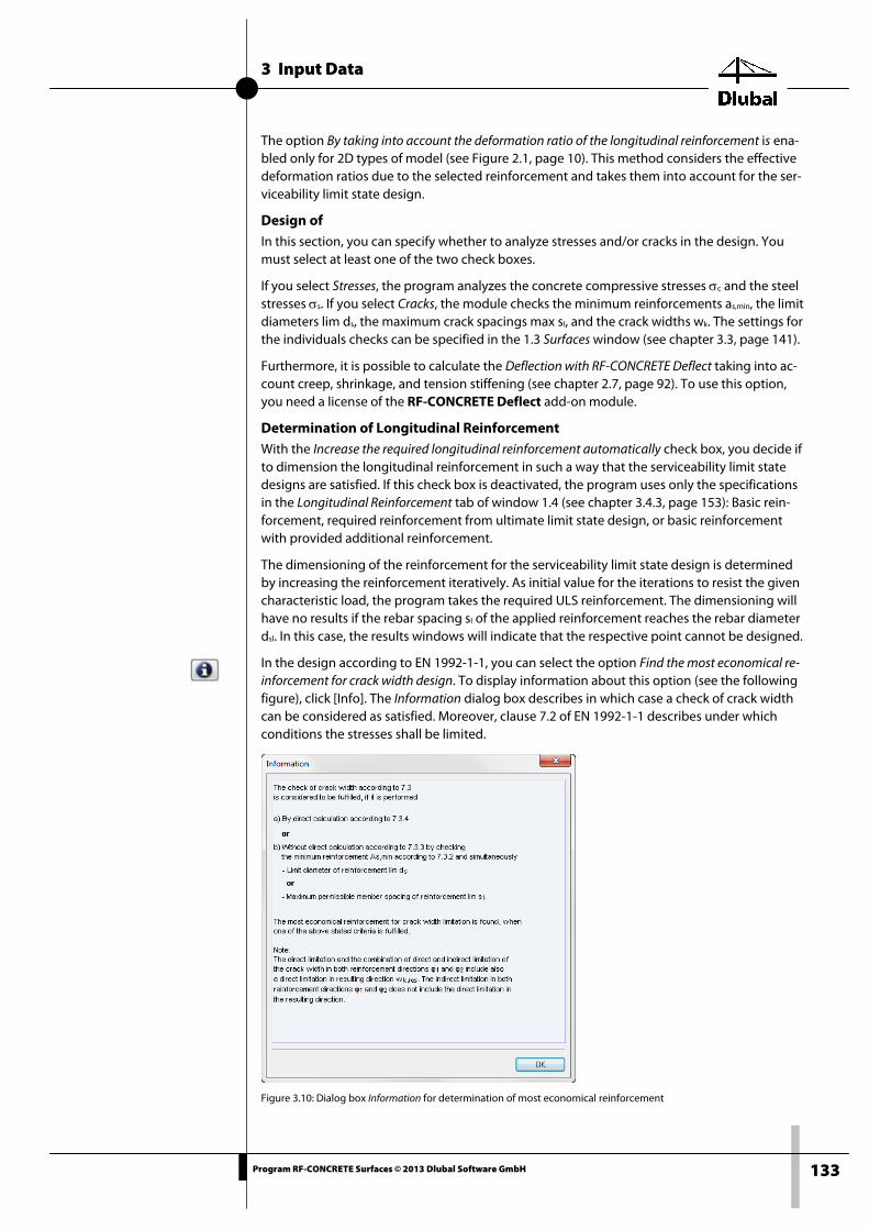
3 Input Data
133 Program RF-CONCRETE Surfaces © 2013 Dlubal Software GmbH
The option By taking into account the deformation ratio of the longitudinal reinforcement is ena-bled only for 2D types of model (see Figure 2.1, page 10). This method considers the effective deformation ratios due to the selected reinforcement and takes them into account for the ser-viceability limit state design.
Design of In this section, you can specify whether to analyze stresses and/or cracks in the design. You must select at least one of the two check boxes.
If you select Stresses, the program analyzes the concrete compressive stresses σc and the steel stresses σs. If you select Cracks, the module checks the minimum reinforcements as,min, the limit diameters lim ds, the maximum crack spacings max sl, and the crack widths wk. The settings for the individuals checks can be specified in the 1.3 Surfaces window (see chapter 3.3, page 141).
Furthermore, it is possible to calculate the Deflection with RF-CONCRETE Deflect taking into ac-count creep, shrinkage, and tension stiffening (see chapter 2.7, page 92). To use this option, you need a license of the RF-CONCRETE Deflect add-on module.
Determination of Longitudinal Reinforcement With the Increase the required longitudinal reinforcement automatically check box, you decide if to dimension the longitudinal reinforcement in such a way that the serviceability limit state designs are satisfied. If this check box is deactivated, the program uses only the specifications in the Longitudinal Reinforcement tab of window 1.4 (see chapter 3.4.3, page 153): Basic rein-forcement, required reinforcement from ultimate limit state design, or basic reinforcement with provided additional reinforcement.
The dimensioning of the reinforcement for the serviceability limit state design is determined by increasing the reinforcement iteratively. As initial value for the iterations to resist the given characteristic load, the program takes the required ULS reinforcement. The dimensioning will have no results if the rebar spacing sl of the applied reinforcement reaches the rebar diameter dsl. In this case, the results windows will indicate that the respective point cannot be designed.
In the design according to EN 1992-1-1, you can select the option Find the most economical re-inforcement for crack width design. To display information about this option (see the following figure), click [Info]. The Information dialog box describes in which case a check of crack width can be considered as satisfied. Moreover, clause 7.2 of EN 1992-1-1 describes under which conditions the stresses shall be limited.
Figure 3.10: Dialog box Information for determination of most economical reinforcement
3 Input Data
134 Program RF-CONCRETE Surfaces © 2013 Dlubal Software GmbH
This means that not all design ratios shown in window 3.1 have to be less than 1 in order for the serviceability limit state design to be fulfilled.
The dimensioning of the reinforcement regarding the concrete and steel stress, the maximum diameters, and the maximum bar spacing is done separately for each reinforcement direction. However, if the resulting crack width wk,res is governing to satisfy the check of crack width, the reinforcement amount is increased equally for each direction.
Criteria of the check that do not have to be satisfied due to economical reasons are indicated in the results windows of the serviceability check by the message 236): "The check of the rein-forcing layers need not be fulfilled for economical reasons." The governing check of crack width for the most economical reinforcement is marked with the message 235): "The check re-stricts increase of reinforcement for economical reasons." This message applies to the designs for lim ds , lim sl, and wk , but not to as,min .
If you select the Find the most economical reinforcement for crack width design, you cannot speci-fy a user-defined additional reinforcement for the SLS design in the Longitudinal Reinforcement tab of the 1.4 Reinforcement window.
Classification Criterion
This section is only available for 3D types of model. With the check boxes, you decide if minor normal forces and/or moments may be neglected in order to design surfaces in an idealized way as pure plates (selection of first check box) or wall (selection of second check box). As limit value, the mean axial tensile strength fctm is preset with 2.9 N/mm2 of a concrete C30/37 for each option: It is assumed that the tensile strength of concrete compensates a crack formation due to minor tensile stresses. This is the reason why they can be neglected.
If you have selected the surface classification as plate or wall in the Method dialog box section on the left, you have to select at least one of the two check boxes.
3.1.2.2 Nonlinear Method In order to perform design according to the Nonlinear method, a license of the add-on module RF-CONCRETE NL is required. This method is described in chapter 2.8, page 107. The program performs a physical and a geometrical nonlinear calculation.
The nonlinear design method assumes an interaction between model and action-effects, re-quiring a clear distribution of internal forces. Therefore, it is only possible to analyze load cases and load combinations, but not result combinations (RC). In a result combination, however, there are two values available for each FE node – maximum and minimum.
The internal forces according to the nonlinear design method are generally determined by second-order analysis.
To open the dialog box for checking and, if necessary, adjusting the design parameters, click [Settings]. This dialog box contains two tabs: Options and Material Properties.

3 Input Data
135 Program RF-CONCRETE Surfaces © 2013 Dlubal Software GmbH
Options
Figure 3.11: Dialog box Settings for Nonlinear Calculation, tab Options
Options
In this section, you select which serviceability limit state designs should be carried out: defor-mation, crack widths, stresses. You must select at least one of the three check boxes.
Furthermore, you can specify if the influence of creep and shrinkage are to be considered in the nonlinear calculation.
Detailed settings for the individual checks as well as for creep and shrinkage are defined in the 1.3 Surfaces window (see chapter 3.3.2, page 144).
Export of Nonlinear Stiffness
With the check box Save the nonlinear stiffness of the defined design load(s) for use in RFEM, you decide if the determined stiffnesses should also be available for a calculation in RFEM.
The stiffnesses can by exported Individually for each designed load case. In the Load Cases and Combinations dialog box of RFEM, you can assign the according stiffness from RF-CONCRETE Surfaces to each of these load cases. RFEM allocates the load cases automatically. If you select the Consistent for reference load option, you must specify the governing load case in the drop-down list below. In RFEM, you can then assign the stiffness resulting from these loads to all defined load cases.
The consideration of nonlinear stiffnesses in RFEM is described in chapter 7.3.1.3 of the RFEM manual.

3 Input Data
136 Program RF-CONCRETE Surfaces © 2013 Dlubal Software GmbH
Settings for Iteration Process
The settings in this section influence the process of the nonlinear design method. For more in-formation, see chapter 2.8.2.4, page 111.
When modifying the precision of iterations, take care that the Maximum number of iterations per load increment is higher than the step in the calculation process from which on the defor-mation criterion will be additionally taken into account. To open the Calculation Parameters dialog box of RFEM, click [Details]. In this dialog box, you can adjust the precision of the con-vergence criteria for the nonlinear calculation.
In the nonlinear calculation, the surface is divided into so-called layers (see chapter 2.8.2.1, page 107). The recommended number of layers is 10.
Moreover, you can influence the performance of the convergence behavior by Damping: The damping controls the magnitude of the stiffness change in the following iteration steps. If you, for example, specify a damping of 50 %, the maximum change of the stiffness between step 2 and 3 can be 50 % of the stiffness change between step 1 and step 2.
Material Properties
Figure 3.12: Dialog box Settings for Nonlinear Calculation, tab Material Properties
Material Properties of Reinforcing Steel
With the check box in this section, you decide if the calculation in the plastic range of the rein-forcing steel's stress-strain diagram will be carried out with a rising or a horizontal graph (see chapter 2.8.3.4, page 119).
Material Properties of Concrete
In this section, you specify the stress-strain relationships of the concrete in compression and tension, respectively. The parabolic diagram for compression and tension stiffening for con-crete tensile stresses are preset in this section.
For tension stiffening (consideration of the stiffening effect of concrete in tension), you can specify the parameters to apply the tensile strength of concrete between the cracks in a sepa-rate dialog box. To open this dialog box, click [Edit].
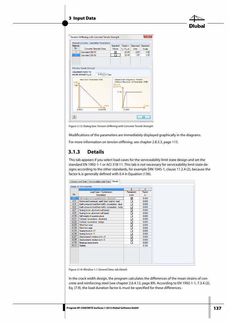
3 Input Data
137 Program RF-CONCRETE Surfaces © 2013 Dlubal Software GmbH
Figure 3.13: Dialog box Tension Stiffening with Concrete Tensile Strength
Modifications of the parameters are immediately displayed graphically in the diagrams.
For more information on tension stiffening, see chapter 2.8.3.3, page 115.
3.1.3 Details This tab appears if you select load cases for the serviceability limit state design and set the standard EN 1992-1-1 or ACI 318-11. This tab is not necessary for serviceability limit state de-signs according to the other standards, for example DIN 1045-1, clause 11.2.4 (2), because the factor kt is generally defined with 0.4 in Equation (136).
Figure 3.14: Window 1.1 General Data, tab Details
In the crack width design, the program calculates the differences of the mean strains of con-crete and reinforcing steel (see chapter 2.6.4.12, page 89). According to EN 1992-1-1, 7.3.4 (2), Eq. (7.9), the load duration factor kt must be specified for these differences.
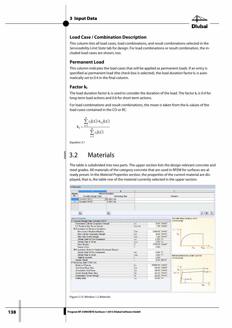
3 Input Data
138 Program RF-CONCRETE Surfaces © 2013 Dlubal Software GmbH
Load Case / Combination Description This column lists all load cases, load combinations, and result combinations selected in the Serviceability Limit State tab for design. For load combinations or result combination, the in-cluded load cases are shown, too.
Permanent Load This column indicates the load cases that will be applied as permanent loads. If an entry is specified as permanent load (the check box is selected), the load duration factor kt is auto-matically set to 0.4 in the final column.
Factor kt
The load duration factor kt is used to consider the duration of the load. The factor kt is 0.4 for long-term load actions and 0.6 for short-term actions.
For load combinations and result combinations, the mean is taken from the kt values of the load cases contained in the CO or RC.
( ) ( )
( )∑
∑
=
=
γ
⋅γ=
n
1ii
n
1ii,ti
t
LC
LCkLC
k
Equation 3.1
3.2 Materials
The table is subdivided into two parts. The upper section lists the design-relevant concrete and steel grades. All materials of the category concrete that are used in RFEM for surfaces are al-ready preset. In the Material Properties section, the properties of the current material are dis-played, that is, the table row of the material currently selected in the upper section.
Figure 3.15: Window 1.2 Materials

3 Input Data
139 Program RF-CONCRETE Surfaces © 2013 Dlubal Software GmbH
The table lists only materials selected for the design. Materials that are not allowed are high-lighted red; changed materials appear blue in color.
Chapter 4.3 of the RFEM manual describes the material properties that are used for the deter-mination of the internal forces. The properties of the materials needed for the design are stored in the global material library. These values are preset for the Concrete Strength Class and the Reinforcing Steel.
To adjust the units and decimal places of material properties and stresses, select Units and Decimal Places in the module's "Settings" menu (see chapter 8.2, page 192).
Material Description
Concrete Strength Class
The concrete materials used in RFEM are already preset; materials that are not relevant are hidden. It is always possible to modify the strength class. To do this, click the material in col-umn A, thus selecting the field. Then, click [] or press [F7] to open the list of the strength classes.
Figure 3.16: List of concrete strength classes
The list contains only strength classes complying with the design concept of the selected standard.
After the transfer, the program shows the updated design-relevant Material Properties.
As a matter of principle, the material properties cannot be edited in RF-CONCRETE Surfaces.
Reinforcing Steel
In this column, the program presets a steel grade that corresponds to the design concept of the selected standard.
Similarly to the concrete strength class, you can select a different reinforcing steel by using the drop-down list: Click the material in column B, thus selecting the field. Then, click [] or press [F7] to open the list with different reinforcing steels.
Figure 3.17: List of reinforcing steels
The list contains only steel grades that are relevant for the selected standard.
After the transfer, the program updates the Material Properties.

3 Input Data
140 Program RF-CONCRETE Surfaces © 2013 Dlubal Software GmbH
Material Library The material library contains many materials. To open the corresponding material library, click the button shown on the left. The buttons are located below column A and B and are used to access the library for the concrete strength classes and reinforcing steels, respectively
Figure 3.18: Dialog box Material Library
In the Filter section, the standard-relevant materials are already preset, thus excluding all other categories or standards. You can select the desired concrete strength class or steel grade from the Material to Select list; then you can check the material properties in the section below.
Click [OK] or press [↵] to transfer the selected material to window 1.2 Materials of RF-CONCRETE Surfaces.
Chapter 4.3 of the RFEM manual describes how to filter, add, or rearrange materials.

3 Input Data
141 Program RF-CONCRETE Surfaces © 2013 Dlubal Software GmbH
3.3 Surfaces
This window lists the surfaces that are relevant for the design.
The makeup of the window depends on the settings in the 1.1 General Data window: If you de-sign the ultimate limit state exclusively, the table lists only the surfaces with their thicknesses. If you have selected load cases for the serviceability limit state design (see Figure 3.8, page 131), however, this window shows specific setting options. They differ depending on the se-lected method of check.
The buttons have the following functions:
Table 3.2: Buttons in window 1.3 Surfaces
3.3.1 Analytical Method The analytical method for the serviceability check is described in chapter 2.6, page 69.
If you use RF-CONCRETE Deflect, this window provides additional tabs and columns. They are described in chapter 3.3.2 Nonlinear Method.
Figure 3.19: Window 1.3 Surfaces with settings for analytical check method, tab Limit of Crack Widths
Button Function
Shows only surfaces that are assigned to a reinforcement group in the 1.4 Reinforcement window (see chapter 3.4)
Jumps to the RFEM work window to adjust the view
Allows you to select a surface in the RFEM work window

3 Input Data
142 Program RF-CONCRETE Surfaces © 2013 Dlubal Software GmbH
Material No. For each surface, the table shows the material numbers that are managed in the 1.2 Materials window.
Thickness
Type
The program is able to design constant and linearly variable thickness types as well as surfaces with orthotropic properties.
d
This column shows the surface thicknesses defined RFEM. The values can be changed for the design.
If the surface thicknesses are modified, the internal forces of RFEM are used for the design, which result from the stiffnesses of the RFEM surface thicknesses. In a statically indeterminate system, the surface thicknesses modified in RF-CONCRETE Surfaces must be also adjusted in RFEM. Thus, the distribution of internal forces is correctly considered in the design.
The other column descriptions are independent of the settings in the tabs below. However, they can be controlled in the Settings dialog box (see Figure 3.9, page 132); in this dialog box, you can specify whether stresses and/or cracks are to be designed.
The values in the columns are based on the entries in the tabs below. These specifications ap-ply to all surfaces by default. It is possible, however, to assign the current specifications only to certain surfaces: Clear the selection in the All check box. Then, enter the numbers of the rele-vant surfaces or select them graphically in the RFEM work window after clicking []. With [], you assign the current settings to these surfaces. However, the assignment is applicable only for the active tab, for example Stress Check.
The two following parameters are defined in the Stress Check tab (see Figure 3.20).
σc,min This column shows the value of the minimum concrete stress for the limitation of the concrete pressure stresses (see chapter 2.6.4.7, page 77). According to EN 1992-1-1, the following applies to
- Quasi-permanent action combination if serviceability, ultimate limit state, or durability are considerably affected by creeping:
σc ≤ 0.45 · fck 7.2 (3)
- Rare ( = characteristic) action combination in exposure classes XD1 to XD3, XF1 to XF4, XS1 to XS3:
σc ≤ 0.60 · fck 7.2 (2)
σs,max This value represents the maximum reinforcing steel stress for the limitation of the reinforce-ment's tensile stresses (see chapter 2.6.4.8, page 80). According to EN 1992-1-1, the following applies to
- Rare action combinations:
σs ≤ 0.80 · fyk 7.2 (5)
- Pure restraint actions:
σs ≤ 1.00 · fyk 7.2 (5)
The remaining parameters are defined in the Limit of Crack Widths tab (see Figure 3.19).

3 Input Data
143 Program RF-CONCRETE Surfaces © 2013 Dlubal Software GmbH
fct,eff
This column displays the respective value of the effective concrete tensile strength. The value is required to control the rebar diameter (see chapter 2.6.4.10, page 84).
wk,-z (top) / wk,+z (bottom) These parameters are allowable crack widths at the top and bottom sides of the surfaces (see chapter 2.6.4.12, page 87).
Restraint If there are effects due to restraint, they shall be considered in the determination of the mini-mum reinforcement to limit the crack width (see chapter 2.6.4.9, page 81).
In the Limit of Crack Widths tab, you can click [Edit] to specify the minimum reinforcement for effects due to restraint (see Figure 2.97, page 82).
Apply
Column I or the check box in the Limitation of Crack Widths tab controls if there are effects due to restraint.
Symbol
In the tab Limitation of Crack Width, you specify whether there are inner or outer effects due to restraint. This has an influence on the factor k taking into account the nonlinearly distributed concrete tensile stresses (see Equation 2.68, page 81).
kc
This factor takes account of the stress distribution in the tension zone (see Equation 2.68, page 81).
Notes This column shows remarks in the form of footers that are described in detail in the status bar.
Comment This input field can be used to enter user-defined comments.

3 Input Data
144 Program RF-CONCRETE Surfaces © 2013 Dlubal Software GmbH
3.3.2 Nonlinear Method To design according to the nonlinear method, you need a license of the RF-CONCRETE NL add-on module. This method for the serviceability limit state design is described in detail in chapter 2.8, page 107.
Figure 3.20: Window 1.3 Surfaces with settings for nonlinear method of check, tab Stress Check
The following columns are described in the chapter above, 3.3.1 Analytical Method:
• Material
• Thickness
• wk,-z / wk,+z
• σc,min
• σs,max
For orthotropic surfaces, no serviceability limit state design according to the nonlinear method is possible.
The values in the columns D through J are controlled in the tabs below. The settings in these tabs are applied to all surfaces by default. It is possible, however, to assign the current specifi-cations only to certain surfaces: Clear the selection of the All check box. Then, enter the num-ber of the relevant surfaces or use [] to select them graphically. With [], you assign the cur-rent settings to these surfaces. The assignment is only applicable for the current tab (for ex-ample Stress Check).
Creep Coefficient ϕ The parameters for creep are defined in the Creeping tab (see Figure 2.144, page 120). Based on these conditions, the program determines the creep coefficient ϕ. For the notional size of the member h0, the program applies the surface thickness d.
The determination of the creep coefficient is described in chapter 2.8.4.1, page 120.
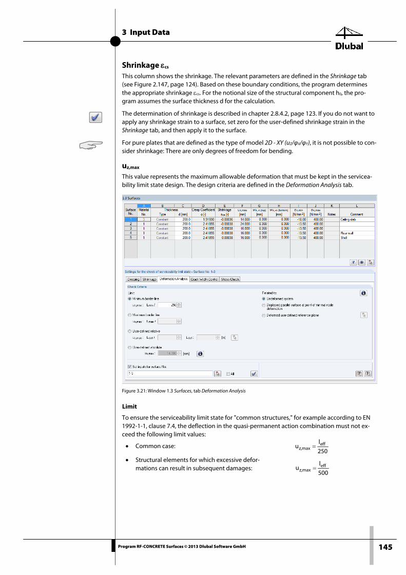
3 Input Data
145 Program RF-CONCRETE Surfaces © 2013 Dlubal Software GmbH
500
lu eff
maxz, =
Shrinkage εcs This column shows the shrinkage. The relevant parameters are defined in the Shrinkage tab (see Figure 2.147, page 124). Based on these boundary conditions, the program determines the appropriate shrinkage εcs. For the notional size of the structural component h0, the pro-gram assumes the surface thickness d for the calculation.
The determination of shrinkage is described in chapter 2.8.4.2, page 123. If you do not want to apply any shrinkage strain to a surface, set zero for the user-defined shrinkage strain in the Shrinkage tab, and then apply it to the surface.
For pure plates that are defined as the type of model 2D - XY (uZ/φX/φY), it is not possible to con-sider shrinkage: There are only degrees of freedom for bending.
uz,max
This value represents the maximum allowable deformation that must be kept in the servicea-bility limit state design. The design criteria are defined in the Deformation Analysis tab.
Figure 3.21: Window 1.3 Surfaces, tab Deformation Analysis
Limit
To ensure the serviceability limit state for "common structures," for example according to EN 1992-1-1, clause 7.4, the deflection in the quasi-permanent action combination must not ex-ceed the following limit values:
• Common case: 250
lu eff
maxz, =
• Structural elements for which excessive defor- mations can result in subsequent damages:
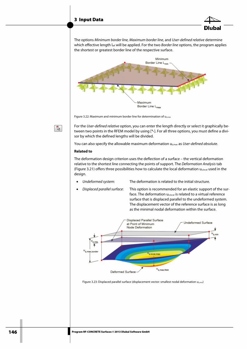
3 Input Data
146 Program RF-CONCRETE Surfaces © 2013 Dlubal Software GmbH
The options Minimum border line, Maximum border line, and User-defined relative determine which effective length leff will be applied. For the two Border line options, the program applies the shortest or greatest border line of the respective surface.
Figure 3.22: Maximum and minimum border line for determination of uz,max
For the User-defined relative option, you can enter the length directly or select it graphically be-tween two points in the RFEM model by using []. For all three options, you must define a divi-sor by which the defined lengths will be divided.
You can also specify the allowable maximum deformation uz,max as User-defined absolute.
Related to
The deformation design criterion uses the deflection of a surface – the vertical deformation relative to the shortest line connecting the points of support. The Deformation Analysis tab (Figure 3.21) offers three possibilities how to calculate the local deformation uz,local used in the design.
• Undeformed system: The deformation is related to the initial structure.
• Displaced parallel surface: This option is recommended for an elastic support of the sur-face. The deformation uz,local is related to a virtual reference surface that is displaced parallel to the undeformed system. The displacement vector of the reference surface is as long as the minimal nodal deformation within the surface.
Figure 3.23: Displaced parallel surface (displacement vector: smallest nodal deformation uz,min)
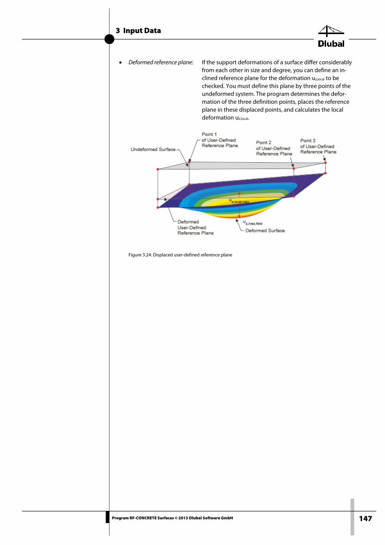
3 Input Data
147 Program RF-CONCRETE Surfaces © 2013 Dlubal Software GmbH
• Deformed reference plane: If the support deformations of a surface differ considerably from each other in size and degree, you can define an in-clined reference plane for the deformation uz,local to be checked. You must define this plane by three points of the undeformed system. The program determines the defor-mation of the three definition points, places the reference plane in these displaced points, and calculates the local deformation uz,local.
Figure 3.24: Displaced user-defined reference plane

3 Input Data
148 Program RF-CONCRETE Surfaces © 2013 Dlubal Software GmbH
3.4 Reinforcement
This window consists of five tabs where all reinforcement data is specified. The individual sur-faces often require different settings. For this purpose, you can define so-called "reinforcement groups" in each RF-CONCRETE Surfaces case. Each reinforcement group contains the reinforce-ment parameters for particular surfaces.
Reinforcement Group To create a new reinforcement group, click [New] in the Reinforcement Group section. The number is automatically assigned by the program. The user-defined Description helps you to overlook all reinforcement groups available in the design case.
Figure 3.25: Window 1.4 Reinforcement with three reinforcement groups
To select the desired reinforcement group, use the No. list or click the entries in the navigator.
By using the [Delete] button, the currently selected reinforcement group is deleted from the design case without any further warning message. Hence, surfaces that were contained in such a reinforcement group will not be designed. If you want to design them, you must reassign them to a new or an existing reinforcement group.
Applied to Surfaces In this dialog box section, you specify the surfaces to which the parameters of the current rein-forcement group apply. By default, All surfaces are selected. If this check box is selected, it is not possible to create any further reinforcement groups. The reason for this is that it is not pos-sible to design a surface by different rules (this is only possible in "design cases," see chapter 8.1, page 190). Therefore, clear the All check box to use several reinforcement groups.
In the input field, enter the number of the surfaces to which the reinforcement parameters of the tabs below apply. You can also select them graphically in the RFEM work window by using the [] function. Only surface numbers that have not yet been assigned to other reinforce-ment groups can be entered in the input field.

3 Input Data
149 Program RF-CONCRETE Surfaces © 2013 Dlubal Software GmbH
3.4.1 Reinforcement Ratios
Figure 3.26: Window 1.4 Reinforcement, tab Reinforcement Ratios
This tab defines the minimum and maximum reinforcements in percentage. The Minimum sec-ondary reinforcement relates to the maximum longitudinal reinforcement that is to be applied. All further reinforcement ratios are related to the cross-sectional area of a surface stripe with the width of one meter.
You can find examples for the minimum and maximum reinforcements in the chapters 2.3.7, 2.4.5, and 2.5.8 of this manual.
3.4.2 Reinforcement Layout
Figure 3.27: Window 1.4 Reinforcement, tab Reinforcement Layout
This tab determines the geometric specifications for the reinforcement.
Number of Reinforcement Directions The reinforcement mesh can be defined with two or three reinforcement directions for each surface side.
For serviceability limit state designs, only a reinforcement mesh with two directions is allowed.

3 Input Data
150 Program RF-CONCRETE Surfaces © 2013 Dlubal Software GmbH
The definition of the "top" and "bottom" side of the surface can be found in the description of the Concrete Cover for Reinforcement section below.
Refer Concrete Cover to
The concrete covers that are defined in the Concrete Cover for Reinforcement section can be re-lated to the reinforcement's Centroid or Edge distance.
Figure 3.28: Reference of the concrete cover
If you select the Edge option, you have to specify the Bar diameter D.
Concrete Cover for Reinforcement For both sides of the surface, you specify the concrete covers of the Basic Reinforcement and, if necessary, the Additional Reinforcement. The dimensions represent either the centroids d of the individual layers or the reinforcements' edge distances cnom in direction ϕ1. The reinforcement directions are defined in the dialog box section below.
The "top" and "bottom" surface side is defined as follows: The bottom surface is defined in di-rection of the positive local surface axis z, the top side is defined in direction of the negative local axis z.
The RFEM graphic shows you the xyz-coordinate systems of the surfaces as soon as you move the pointer across a surface. You can also use the context menu of a surface (right-click it) to switch the axes on and off.
Figure 3.29: RFEM context menu of an area

3 Input Data
151 Program RF-CONCRETE Surfaces © 2013 Dlubal Software GmbH
Selection of the exposure class
To display the surface sides in different colors, select Colors in Rendering According to → +/- z-Surface sides in the Display navigator (see figure on the left).
You can change the orientation of the local z-axis of a surface by using the Reverse Local Axis System option on the context menu (see Figure 3.29). In this way, it is possible to unify, for ex-ample, the orientation of walls in order to assign the top and bottom reinforcement sides for vertical surfaces unambiguously.
The model types wall 2D - XZ (uX/uZ/φY) or 2D - XY (uX/uY/φZ) are models whose component's plane is exclusively subjected to compression or tension, respectively. In this case, it is not pos-sible to create different reinforcement meshes for each surface side so that the input possibili-ties are limited to uniform concrete covers on both sides.
If you select the According to Standard check box, the [Edit] button becomes available. Click [Edit] to open the following dialog box.
Figure 3.30: Dialog box Cover acc. to Standard
In the upper section, you can define the parameters for the design (exposure class, abrasion class, etc.) according to the standard. From these parameters, RF-CONCRETE Surfaces deter-mines the required concrete cover.
In the two tabs, you can specify the parameters for each surface side separately.

3 Input Data
152 Program RF-CONCRETE Surfaces © 2013 Dlubal Software GmbH
Reinforcement Directions Related to Local Axis x of FE-Element The reinforcement directions ϕ are related to the local x-axis of the finite elements. In the Edit Surface dialog box of RFEM, you can check and, if necessary, adjust the axes system for the re-sults of the surfaces.
Figure 3.31: RFEM dialog box Edit Surface, tab Axes and Axes for Results
For curved surfaces, it is recommended to check the axes of the finite elements graphically: In the Display navigator of RFEM, select the option FE Mesh → On Surfaces → FE Axis Systems x,y,z → Indexes (see Figure 8.40 in chapter 8.14 of the RFEM manual).
The reinforcement directions are to be specified by means of the angle ϕ for each layer. Only positive angles are allowed. They represent the respective clockwise rotation of the reinforce-ment direction in relation to the corresponding x-axis.
For the model types wall 2D - XZ (uX/uZ/φY) or 2D - XY (uX/uY/φZ), it is not possible to create differ-ent reinforcement meshes for each side of the surface. Thus, the input options are limited to uniform reinforcement directions on both surface sides.
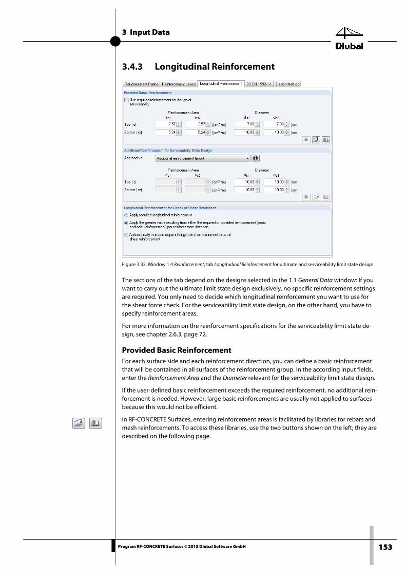
3 Input Data
153 Program RF-CONCRETE Surfaces © 2013 Dlubal Software GmbH
3.4.3 Longitudinal Reinforcement
Figure 3.32: Window 1.4 Reinforcement, tab Longitudinal Reinforcement for ultimate and serviceability limit state design
The sections of the tab depend on the designs selected in the 1.1 General Data window: If you want to carry out the ultimate limit state design exclusively, no specific reinforcement settings are required. You only need to decide which longitudinal reinforcement you want to use for the shear force check. For the serviceability limit state design, on the other hand, you have to specify reinforcement areas.
For more information on the reinforcement specifications for the serviceability limit state de-sign, see chapter 2.6.3, page 72.
Provided Basic Reinforcement For each surface side and each reinforcement direction, you can define a basic reinforcement that will be contained in all surfaces of the reinforcement group. In the according input fields, enter the Reinforcement Area and the Diameter relevant for the serviceability limit state design.
If the user-defined basic reinforcement exceeds the required reinforcement, no additional rein-forcement is needed. However, large basic reinforcements are usually not applied to surfaces because this would not be efficient.
In RF-CONCRETE Surfaces, entering reinforcement areas is facilitated by libraries for rebars and mesh reinforcements. To access these libraries, use the two buttons shown on the left; they are described on the following page.
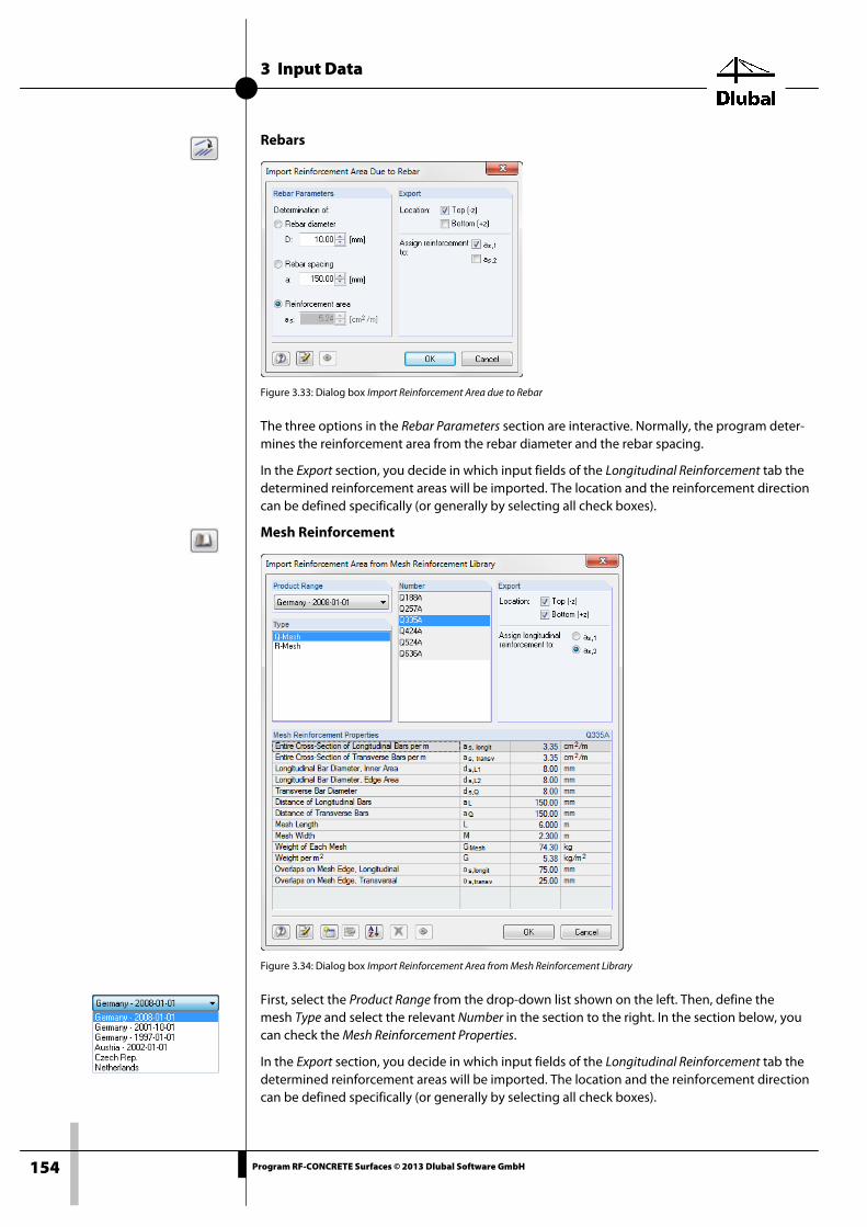
3 Input Data
154 Program RF-CONCRETE Surfaces © 2013 Dlubal Software GmbH
Rebars
Figure 3.33: Dialog box Import Reinforcement Area due to Rebar
The three options in the Rebar Parameters section are interactive. Normally, the program deter-mines the reinforcement area from the rebar diameter and the rebar spacing.
In the Export section, you decide in which input fields of the Longitudinal Reinforcement tab the determined reinforcement areas will be imported. The location and the reinforcement direction can be defined specifically (or generally by selecting all check boxes).
Mesh Reinforcement
Figure 3.34: Dialog box Import Reinforcement Area from Mesh Reinforcement Library
First, select the Product Range from the drop-down list shown on the left. Then, define the mesh Type and select the relevant Number in the section to the right. In the section below, you can check the Mesh Reinforcement Properties.
In the Export section, you decide in which input fields of the Longitudinal Reinforcement tab the determined reinforcement areas will be imported. The location and the reinforcement direction can be defined specifically (or generally by selecting all check boxes).

3 Input Data
155 Program RF-CONCRETE Surfaces © 2013 Dlubal Software GmbH
Use required reinforcement for design of serviceability
The ideal way to perform the serviceability limit state design would be the following:
1. Determine the required reinforcement by using only the load specified in the tab Ultimate Limit State.
2. Create a reinforcement drawing including mesh reinforcements and rebars on the bases of the colored result diagram.
3. If necessary, divide the surfaces based on the reinforcement drawing into smaller surfaces that have the same provided reinforcement area in each reinforcement direction.
4. Define the provided reinforcement area, rebar spacing, and diameter for each surface in RF-CONCRETE Surfaces.
5. Recalculate with the loads in the tab Serviceability Limit State.
This procedure is cumbersome and runs contrary to the convention stating that you can de-termine the reinforcement and perform the serviceability limit state designs at the same time by simply using the [Calculation] button.
Therefore, you can select the check box Use required design reinforcement for design of servicea-bility to quickly obtain a provided reinforcement for the individual surfaces: The program uses the required reinforcement from the ultimate limit state design as the reinforcement to be ap-plied. If the check box is selected, you only need to specify the rebar diameter.
Additional Reinforcement for Serviceability Limit State Design In the areas where the statically required reinforcement exceeds the basic reinforcement, an additional reinforcement is needed. Use the drop-down list to specify which additional rein-forcement is applied for the serviceability limit state design.
If you select the Required additional reinforcement option, the actual As,req distribution is applied as additional reinforcement in the SLS design.
The Additional reinforcement layout is determined as difference between the greater statically required reinforcement of all surfaces of the reinforcement group and the defined basic rein-forcement:
as,add = max as,req – as,basic
Equation 3.2
Click [Info] to open the dialog box illustrating the additional reinforcement (see Figure 3.35).
To dimension the additional reinforcement, you only need to specify the rebar diameter.
You can also specify a User-defined additional reinforcement. For this, the program offers librar-ies for the rebars and mesh reinforcements, just as in the Provided Basic Reinforcement section.

3 Input Data
156 Program RF-CONCRETE Surfaces © 2013 Dlubal Software GmbH
Figure 3.35: Applying additional reinforcement
Longitudinal Reinforcement for Check of Shear Resistance The last section provides options to define the longitudinal reinforcement to be applied for the shear check without shear reinforcement.
Figure 3.36: Longitudinal reinforcement for check of shear resistance
• Apply required longitudinal reinforcement
The check of shear resistance is carried out with the transformed provided tension rein-forcement in direction of the principal shear force (see chapter 2.4.4.1, page 39).
• Apply the greater value resulting from either the required or provided reinforcement (basic and add. reinforcement) per reinforcement direction
For the check of shear resistance, the program uses either the statically required or the user-defined longitudinal reinforcement (see chapter 2.4.4.1, page 42).
• Automatically increase required longitudinal reinforcement to avoid shear reinforcement
If the required longitudinal reinforcement is not sufficient for the shear force resistance, the longitudinal reinforcement will be increased in the main shear force direction until the shear check without shear reinforcement is satisfied (see chapter 2.4.4.1, page 40).

3 Input Data
157 Program RF-CONCRETE Surfaces © 2013 Dlubal Software GmbH
3.4.4 Standard The parameters of this tab depend on the standard selected in the 1.1 General Data window. In this tab, you specify the standard-specific reinforcement data. In the following, this is de-scribed for EN 1992-1-1.
At the bottom right below the table, two buttons are available. Click [Default] to reset the ini-tial values of the current standard. Use [Set As Default] to store the defined entries as new de-fault settings.
Figure 3.37: Window 1.4 Reinforcement, tab BS EN 1992-1-1
Minimum Reinforcement In this section, you decide which provisions of the standard regarding the minimum reinforce-ment are to be considered in the design (see chapter 2.3.7, page 25).
For plates and walls, click [Settings] to set the direction of the minimum and main compression reinforcement.
Plates
Figure 3.38: Dialog box Settings for Min. Reinforcement for Ductile Properties
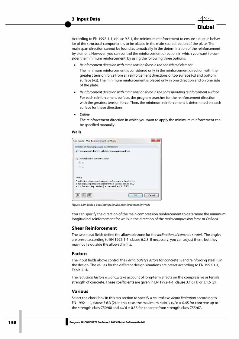
3 Input Data
158 Program RF-CONCRETE Surfaces © 2013 Dlubal Software GmbH
According to EN 1992-1-1, clause 9.3.1, the minimum reinforcement to ensure a ductile behav-ior of the structural component is to be placed in the main span direction of the plate. The main span direction cannot be found automatically in the determination of the reinforcement by element. However, you can control the reinforcement direction, in which you want to con-sider the minimum reinforcement, by using the following three options:
• Reinforcement direction with main tension force in the considered element
The minimum reinforcement is considered only in the reinforcement direction with the greatest tension force from all reinforcement directions of top surface (-z) and bottom surface (+z): The minimum reinforcement is placed only in one direction and on one side of the plate.
• Reinforcement direction with main tension force in the corresponding reinforcement surface
For each reinforcement surface, the program searches for the reinforcement direction with the greatest tension force. Then, the minimum reinforcement is determined on each surface for these directions.
• Define
The reinforcement direction in which you want to apply the minimum reinforcement can be specified manually.
Walls
Figure 3.39: Dialog box Settings for Min. Reinforcement for Walls
You can specify the direction of the main compression reinforcement to determine the minimum longitudinal reinforcement for walls in the direction of the main compression force or Defined.
Shear Reinforcement The two input fields define the allowable zone for the inclination of concrete strutsθ. The angles are preset according to EN 1992-1-1, clause 6.2.3. If necessary, you can adjust them, but they may not lie outside the allowed limits.
Factors The input fields above control the Partial Safety Factors for concrete γc and reinforcing steel γs in the design. The values for the different design situations are preset according to EN 1992-1-1, Table 2.1N.
The reduction factors αcc or αct take account of long-term effects on the compressive or tensile strength of concrete. These coefficients are given in EN 1992-1-1, clause 3.1.6 (1) or 3.1.6 (2).
Various Select the check box in this tab section to specify a neutral axis depth limitation according to EN 1992-1-1, clause 5.6.3 (2). In this case, the maximum ratio is xd / d = 0.45 for concrete up to the strength class C50/60 and xd / d = 0.35 for concrete from strength class C55/67.

3 Input Data
159 Program RF-CONCRETE Surfaces © 2013 Dlubal Software GmbH
3.4.5 Design Method
Figure 3.40: Window 1.4 Reinforcement, tab Design Method
In determining the required reinforcement, the principal internal forces are transformed into design forces (in direction of the reinforcement) and in a related concrete strut force. The sizes of these design forces depend on the presumed angle of the concrete strut that braces the re-inforcement mesh.
In the load situations "tension-tension" and "tension-compression" (see Figure 2.19, page 22), the design force may become negative in one reinforcement direction for a certain inclination of the concrete strut, that is, compressive forces would occur for the tension reinforcement. Due to the optimization of design forces, the direction of the concrete strut is modified until the negative design force is zero.
In the optimization process of internal forces, the program determines the inclination angle of the concrete strut that produces the most favorable design result. The design moments are determined iteratively with adjusted inclination angles in order to find the smallest energy with the least required reinforcement. The optimization process is described in an example in chapter 2.4.1, page 28.
The optimization for concrete components subjected to compression (such as walls) may re-sult in non-designable elements due to failure of the compression strut. Therefore, the optimi-zation is not recommended for the load situation "compression-compression".

4 Calculation
160 Program RF-CONCRETE Surfaces © 2013 Dlubal Software GmbH
4. Calculation In RF-CONCRETE Surfaces, the [Calculation] is carried out with the internal forces from RFEM. If the RFEM results are not yet available, the program starts the calculation of the internal forces automatically.
4.1 Details Click the [Details] button, which is available in the 1.1 General Data window, to open the corre-sponding dialog box where you can influence the design of result combinations, several load cases or combinations, as well as of the internal forces in the average and rip regions.
The following dialog box opens.
Figure 4.1: Dialog box Details
Analysis Method for Result Combinations This section controls how the design internal forces of the result combinations are included in the calculation. This specification also applies when there are several load cases or load com-binations in the design case to be analyzed. The Mixed Method is preset: Before the design, the program analyzes whether the Enumeration Method or the Envelope Method needs less compu-tation time.
Enumeration Method
Each load case and each load combination selected in the 1.1 General Data window is designed individually. From the results, the reinforcement envelope is computed. For result combina-tions, 16 calculations are performed for the RFEM extreme values of the basic internal forces max/min mx, max/min nx, max/min my, max/min ny, max/min mxy, max/min nxy, max/min vx, and max/min vy.
The Enumeration Method is very precise because every combination is calculated separately, and then the enveloping reinforcement is determined. However, the disadvantage of this method is that the number of the combinations to be analyzed increases exponentially with the number of load cases, as the program proceeds from row to row. Thus, if there are, for ex-ample, 50 selected load combinations, there will also be 50 reinforcement designs. On the other hand, all possible variants (constellations) are included in the designs.
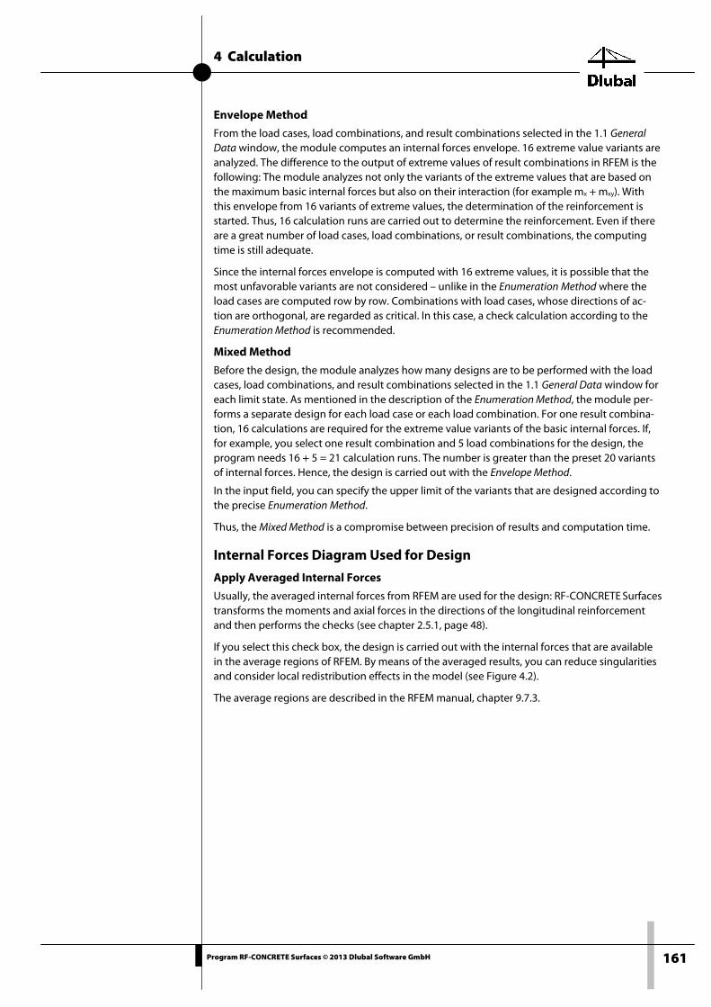
4 Calculation
161 Program RF-CONCRETE Surfaces © 2013 Dlubal Software GmbH
Envelope Method
From the load cases, load combinations, and result combinations selected in the 1.1 General Data window, the module computes an internal forces envelope. 16 extreme value variants are analyzed. The difference to the output of extreme values of result combinations in RFEM is the following: The module analyzes not only the variants of the extreme values that are based on the maximum basic internal forces but also on their interaction (for example mx + mxy). With this envelope from 16 variants of extreme values, the determination of the reinforcement is started. Thus, 16 calculation runs are carried out to determine the reinforcement. Even if there are a great number of load cases, load combinations, or result combinations, the computing time is still adequate.
Since the internal forces envelope is computed with 16 extreme values, it is possible that the most unfavorable variants are not considered – unlike in the Enumeration Method where the load cases are computed row by row. Combinations with load cases, whose directions of ac-tion are orthogonal, are regarded as critical. In this case, a check calculation according to the Enumeration Method is recommended.
Mixed Method
Before the design, the module analyzes how many designs are to be performed with the load cases, load combinations, and result combinations selected in the 1.1 General Data window for each limit state. As mentioned in the description of the Enumeration Method, the module per-forms a separate design for each load case or each load combination. For one result combina-tion, 16 calculations are required for the extreme value variants of the basic internal forces. If, for example, you select one result combination and 5 load combinations for the design, the program needs 16 + 5 = 21 calculation runs. The number is greater than the preset 20 variants of internal forces. Hence, the design is carried out with the Envelope Method.
In the input field, you can specify the upper limit of the variants that are designed according to the precise Enumeration Method.
Thus, the Mixed Method is a compromise between precision of results and computation time.
Internal Forces Diagram Used for Design
Apply Averaged Internal Forces
Usually, the averaged internal forces from RFEM are used for the design: RF-CONCRETE Surfaces transforms the moments and axial forces in the directions of the longitudinal reinforcement and then performs the checks (see chapter 2.5.1, page 48).
If you select this check box, the design is carried out with the internal forces that are available in the average regions of RFEM. By means of the averaged results, you can reduce singularities and consider local redistribution effects in the model (see Figure 4.2).
The average regions are described in the RFEM manual, chapter 9.7.3.

4 Calculation
162 Program RF-CONCRETE Surfaces © 2013 Dlubal Software GmbH
Figure 4.2: Top reinforcement for unaveraged internal forces (left) and average regions across columns (right)
Apply Internal Forces Without Rib Components
In RFEM, you can model a T-beam by using a surface and an eccentrically connected member of the "rib" type. The internal forces of the T-beam from surface component and member are determined by integration of the internal forces in surfaces as rib internal forces.
With the final check box, you decide whether the surface internal forces assigned to the rib are included in the surface design. The design with the rib component is preset.
4.2 Check Before you start the calculation, it is recommended to check if the input data is correct. The [Check] button is available in every input window of RF-CONCRETE Surfaces.
The program checks if the data required for the design is complete and if the references of the data sets are alright. If the program does not detect any input errors, it displays the following message:
Figure 4.3: Plausibility check

4 Calculation
163 Program RF-CONCRETE Surfaces © 2013 Dlubal Software GmbH
4.3 Start Calculation You can start the calculation out of each input window of the RF-CONCRETE Surfaces module by clicking [Calculation].
RF-CONCRETE Surfaces searches for the results of the load cases, load combinations, and result combinations that you want to design. If they cannot be found, the program starts the RFEM calculation to determine the design-relevant internal forces.
You can also start the calculation out of the RFEM user interface: The To Calculate dialog box (menu Calculate → To Calculate) lists the design cases of the add-on modules like load cases or load combinations.
Figure 4.4: Dialog box To Calculate
If the design cases of RF-CONCRETE Surfaces are missing in the Not Calculated section, select All or Add-on Modules from the drop-down list below the section.
To transfer the selected RF-CONCRETE Surfaces cases to the dialog box section on the right, click []. To start the calculation, click [OK].
Alternatively, you can use the drop-down list in the toolbar to calculate a design case: Select the RF-CONCRETE Surfaces case, and then click [Show Results].
Figure 4.5: Direct calculation of an RF-CONCRETE Surfaces design case in RFEM
Subsequently, you can observe the calculation process in the solver dialog box.

5 Results
164 Program RF-CONCRETE Surfaces © 2013 Dlubal Software GmbH
5. Results The 2.1 Required Reinforcement Total window is displayed immediately after the calculation.
Figure 5.1: Results window
The ultimate limit state designs are listed in the results windows 2.1 through 2.3 by various criteria.
The windows 3.1 through 3.3 contain the results of the serviceability limit state designs.
All windows can be selected directly by clicking the according entry in the navigator. Use the buttons shown on the left to go to the previous or next window. You can also use the function keys [F2] and [F3] to select the previous or next window.
At the bottom of the windows, you find two option buttons. With these buttons, you decide whether to show the results data In FE nodes or In grid points. The results of the FE nodes are determined directly by the analysis core. The grid point results are determined by interpola-tion of the FE node results.
To save the results, click [OK]. Thus, you exit RF-CONCRETE Surfaces and return to the main program.
Chapter 5 Results presents the results windows in their proper order. Evaluating and checking results is described in chapter 6 Results Evaluation, page 176.

5 Results
165 Program RF-CONCRETE Surfaces © 2013 Dlubal Software GmbH
5.1 Required Reinforcement Total The table shows the maximum reinforcement areas of all analyzed surfaces. The areas are de-termined from the internal forces of the load cases, load combinations, and result combina-tions selected for the ultimate limit state design.
Figure 5.2: Window 2.1 Required Reinforcement Total
Surface No. The column shows the numbers of surfaces containing the governing points.
Point No. / Grid Point In these FE nodes or grid points, the greatest required reinforcement was determined for each position and direction. The reinforcement type is displayed in column E Symbol.
The FE mesh nodes M are generated automatically. In contrast to this, the grid points G can be controlled in RFEM, as user-defined result grids are possible for surfaces. The function is de-scribed in chapter 8.12 of the RFEM manual.
Point Coordinates X/Y/Z The three columns show the coordinates of the governing FE nodes or grid points.
Symbol Column E displays the reinforcement type. For the four (or six) longitudinal reinforcements, the module shows the directions (1, 2 and 3, if available) as well as the surface sides (top and bottom).
The reinforcement directions are defined in the Reinforcement Layout tab of the 1.4 Reinforce-ment window (see chapter 3.4.2, page 149).
The top reinforcement is defined on the surface side in direction of the negative local surface axis z (-z). Accordingly, the top reinforcement is defined in direction of the positive z-axis (+z). The Figure 3.29 on page 150 shows the axis systems of the surfaces.
The shear reinforcement is indicated as asw.
Top and bottom surface
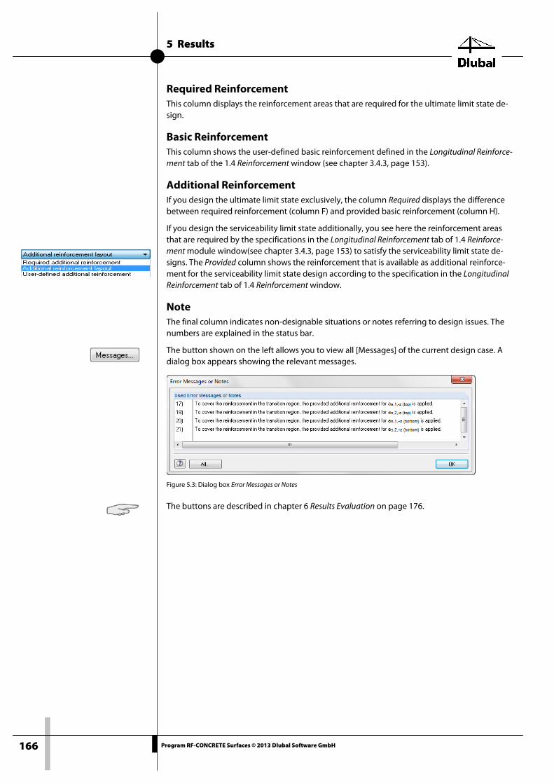
5 Results
166 Program RF-CONCRETE Surfaces © 2013 Dlubal Software GmbH
Required Reinforcement This column displays the reinforcement areas that are required for the ultimate limit state de-sign.
Basic Reinforcement This column shows the user-defined basic reinforcement defined in the Longitudinal Reinforce-ment tab of the 1.4 Reinforcement window (see chapter 3.4.3, page 153).
Additional Reinforcement If you design the ultimate limit state exclusively, the column Required displays the difference between required reinforcement (column F) and provided basic reinforcement (column H).
If you design the serviceability limit state additionally, you see here the reinforcement areas that are required by the specifications in the Longitudinal Reinforcement tab of 1.4 Reinforce-ment module window(see chapter 3.4.3, page 153) to satisfy the serviceability limit state de-signs. The Provided column shows the reinforcement that is available as additional reinforce-ment for the serviceability limit state design according to the specification in the Longitudinal Reinforcement tab of 1.4 Reinforcement window.
Note The final column indicates non-designable situations or notes referring to design issues. The numbers are explained in the status bar.
The button shown on the left allows you to view all [Messages] of the current design case. A dialog box appears showing the relevant messages.
Figure 5.3: Dialog box Error Messages or Notes
The buttons are described in chapter 6 Results Evaluation on page 176.

5 Results
167 Program RF-CONCRETE Surfaces © 2013 Dlubal Software GmbH
5.2 Required Reinforcement by Surface
Figure 5.4: Window 2.2 Required Reinforcement by Surface
This window shows the maximum reinforcement areas that are required for each of the de-signed surfaces. The columns are described in chapter 5.1.

5 Results
168 Program RF-CONCRETE Surfaces © 2013 Dlubal Software GmbH
5.3 Required Reinforcement by Point
Figure 5.5: Window 2.3 Required Reinforcement by Point
This results window lists the maximum reinforcement areas for all FE nodes or grid points of each surface. The columns are described in detail in chapter 5.1.
In addition to the longitudinal and shear reinforcements, the table display design-relevant values of the actions and resistances. For EN 1992-1-1, these are the following:
Symbol Meaning
n1,-z (top) Axial force or membrane force for design of reinforcement in first reinforce-ment direction on top side of the surface
n2,-z (top) Axial force or membrane force for design of reinforcement in second rein-forcement direction on top side of the surface
n1,+z (bottom) Same as n1,-z (top), but on bottom side of the surface
n2,+z (bottom) Same as n2,-z (top), but on bottom side of the surface
m1,-z (top) m2,-z (top)
Only for type of model 2D - XY (uZ/φX/φY): moment for design of reinforce-ment in first or second reinforcement direction on top side of the surface
m1,-z (bottom)
m2,-z (bottom) Same as m1,-z (top) / m2,-z (top), but on bottom side of the surface
VEd Design value of applied shear force
VRd,c Design shear resistance without shear reinforcement
VRd,max Design shear resistance of concrete strut
VRd,s Design shear resistance of shear reinforcement
Theta Inclination angle of concrete strut θ
Table 5.1: Output values in window 2.3 for EN 1992-1-1

5 Results
169 Program RF-CONCRETE Surfaces © 2013 Dlubal Software GmbH
The search function, which you can start by clicking the button shown on the left, helps you find specific FE nodes or grid points quickly (see Figure 6.7, page 182).
5.4 Serviceability Checks Total The upper part of the window shows a summary of the governing serviceability limit state de-signs. The lower part displays the intermediate results of the current FE node or grid point (that is, of the point selected in the upper table) including all design-relevant parameters. You can expand or reduce the entries by clicking [+] or [-], respectively.
Figure 5.6: Window 3.1 Serviceability Checks Total
Figure 5.6 shows the results window of an analytical serviceability limit state check. Chapter 5.7 on page 173 describes the results windows that appear when a nonlinear serviceability limit state calculation was carried out.
The method of check is defined in the Serviceability Limit State tab of the 1.1General Data win-dow (see Figure 3.8, page 131).
Surface No. The column shows the numbers of surfaces containing the governing points.
Point No. / Grid Point These FE nodes or grid points provide the maximum ratios for the required checks. The type of check is displayed in column F Symbol.
The FE mesh nodes M are generated automatically. The grid points G can be controlled in RFEM (see chapter 8.12 of the RFEM manual).
Point Coordinates X/Y/Z The three columns show the coordinates of the governing FE nodes or grid points.

5 Results
170 Program RF-CONCRETE Surfaces © 2013 Dlubal Software GmbH
Loading Column E displays the load cases, load or result combinations whose internal forces produce the greatest ratios for the respective serviceability limit state design.
Symbol Column F shows the type of the serviceability limit state design. If you have selected the ana-lytical method, this column will show up to six types of check. These types are described by an example in chapter 2.6.4, page 77.
The symbols stand for the following types of checks:
Symbol Design SLS
σc Limitation of concrete compressive stress ( chapter 2.6.4.7, page 77) according to specifications in the 1.3 Surfaces window (see Figure 3.20, page 144)
σs Limitation of reinforcing steel stress ( chapter 2.6.4.8, page 80) according to specifications in the 1.3 Surfaces window (see Figure 3.19, page 141)
as,min Minimum reinforcement for crack width limitation ( chapter 2.6.4.9, page 81) according to specifications in the 1.3 Surfaces window (see Figure 2.97, page 82)
lim ds Limitation of rebar diameter ( chapter 2.6.4.10, page 84) according to specifi-cations in the 1.4 Surfaces window (see Figure 3.32, page 153)
lim sl Limitation of rebar spacing ( chapter 2.6.4.11, page 86) according to specifica-tions in the 1.4 Surfaces window (see Figure 3.32, page 153)
wk Limitation of crack width ( chapter 2.6.4.12, page 87) according to specifica-tions in the 1.3 Surfaces window (see Figure 3.19, page 141)
Table 5.2: Serviceability limit state designs according to analytical method
Existing Value This column displays the values of all surfaces that are governing for the serviceability limit state designs.
Limit Value The design limit values are determined from the standard specifications and the load situation. The determination of the limit values is described in chapter 2.6.4, page 77f.
Ratio Column J shows the ratio of the existing value (column G) and the limit value (column H). Rati-os greater than 1 mean that the design criterion is not satisfied. The length of the colored scale illustrates the respective ratio graphically.
For the serviceability limit state designs, not all types of checks must be satisfied (see explana-tion in Figure 3.10, page 133).
Note The final column indicates non-designable situations or notes referring to design issues. The numbers are explained in the status bar.
To display all messages of the currently selected design case, use the [Messages] button shown on the left. A dialog box showing the relevant messages appears (see Figure 5.3, page 166).
The buttons are described in chapter 6 Results Evaluation, page 176.

5 Results
171 Program RF-CONCRETE Surfaces © 2013 Dlubal Software GmbH
5.5 Serviceability Checks by Surface
Figure 5.7: Window 3.2 Serviceability Checks by Surface
This window lists the maximum ratios of each designed surface resulting for the serviceability limit state designs. The columns are described in detail in chapter 5.4.

5 Results
172 Program RF-CONCRETE Surfaces © 2013 Dlubal Software GmbH
5.6 Serviceability Checks by Point
Figure 5.8: Window 3.3Serviceability Checks by Point
This results window lists the maximum ratios for all FE nodes or grid points of each surface. The columns are described in detail in chapter 5.4.
The search function, which you can start by clicking the button shown on the left, helps you find specific FE nodes or grid points quickly (see Figure 6.7, page 182).

5 Results
173 Program RF-CONCRETE Surfaces © 2013 Dlubal Software GmbH
5.7 Nonlinear Calculation Total The upper part of the window presents a summary of the governing serviceability limit state designs. The lower part displays the intermediate results of the current FE nodes or grid point (that is, the entry selected above) including all design-relevant parameters. You can expand or reduce the entries by clicking [+] or [-], respectively.
Figure 5.9: Window 3.1 Nonlinear Calculation Total
Figure 5.9 shows the results window of a nonlinear serviceability limit state design. The meth-od of check is specified in the Serviceability Limit State tab of the 1.1 General Data window (see Figure 3.8, page 131).
The columns are described in chapter 5.4, page 169.
The symbols stand for the following types of checks individual types of check:
Symbol Design SLS
uz,local Deformation in cracked state ( chapter 2.8.2.4, page 111) according to specifi-cations in the window 1.3 Surfaces
wk Limitation of crack width ( chapter 2.6.4.12, page 87) according to specifica-tions in the 1.3 Surfaces window (see Figure 3.19, page 141)
σc Limitation of concrete compression stress ( chapter 2.6.4.7, page 77) according to specifications in the 1.3 Surfaces window (see Figure 3.20, page 144)
σs Limitation of reinforcing steel stress ( chapter 2.6.4.8, page 80) according to specifications in the 1.3 Surfaces window (see Figure 3.20, page 144)
Table 5.3: Serviceability limit state designs according to nonlinear method
The values of the deformations, crack widths, and stresses represent the results in cracked sec-tions (state II).
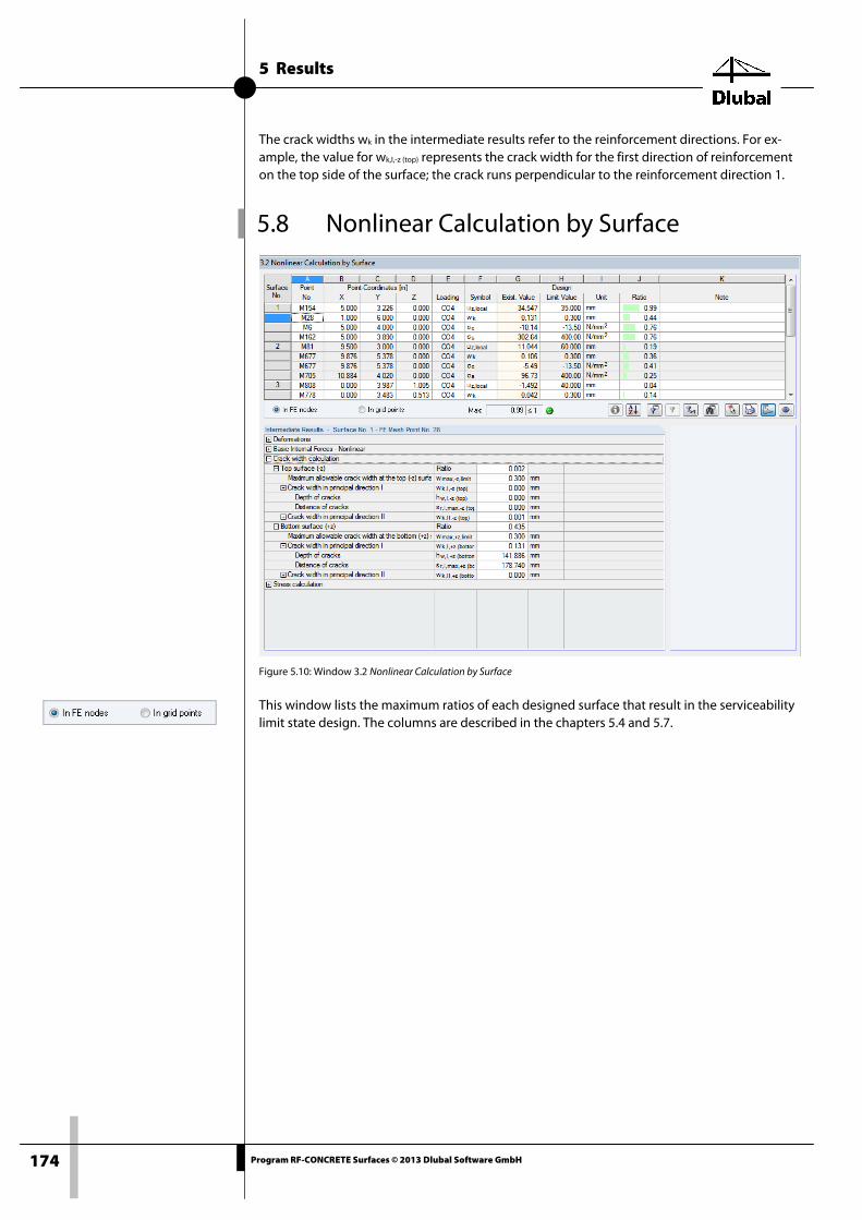
5 Results
174 Program RF-CONCRETE Surfaces © 2013 Dlubal Software GmbH
The crack widths wk in the intermediate results refer to the reinforcement directions. For ex-ample, the value for wk,I,-z (top) represents the crack width for the first direction of reinforcement on the top side of the surface; the crack runs perpendicular to the reinforcement direction 1.
5.8 Nonlinear Calculation by Surface
Figure 5.10: Window 3.2 Nonlinear Calculation by Surface
This window lists the maximum ratios of each designed surface that result in the serviceability limit state design. The columns are described in the chapters 5.4 and 5.7.

5 Results
175 Program RF-CONCRETE Surfaces © 2013 Dlubal Software GmbH
5.9 Nonlinear Calculation by Point
Figure 5.11: Window 3.3 Nonlinear Calculation by Point
This results window lists the maximum ratios for all FE nodes or grid points of each surface. The columns are described in the chapters 5.4 and 5.7.
The search function that you can start by clicking the button shown on the left helps you find FE nodes or grid points quickly (see Figure 6.7, page 182).

6 Results Evaluation
176 Program RF-CONCRETE Surfaces © 2013 Dlubal Software GmbH
6. Results Evaluation The design results can be evaluated in various ways. For this purpose, you can use the buttons below the tables.
Figure 6.1: Buttons for results evaluation
The buttons have the following functions:
Button Description Function
Design Details Opens the dialog box Design Details chapter 6.1, page 177
Sorts Results Sorts the results by the maximum ratios (column J) or maximum values (column G) chapter 6.3, page 182
Filter Opens the Filter Points dialog box to select FE nodes or grid points by certain criteria chapter 6.3, page 182
Only Designable Results Hides the rows with the non-designable situations
Exceeding Shows only rows with a ratio > 1 (design not fulfilled)
Find Opens the Find FE Node / Grid Point dialog box to find a certain results row chapter 6.3, page 182
Surface Selection Allows you to graphically select a surface to show its results in the table
Print Includes the intermediate results of the current FE node or grid point in printout report
Show Color Bars Shows or hides the colored reference scales in the results windows
View Mode Jumps to the RFEM work window to adjust the view
Table 6.1: Buttons in the results windows

6 Results Evaluation
177 Program RF-CONCRETE Surfaces © 2013 Dlubal Software GmbH
6.1 Design Details Click [Info] (available in all results windows) to check on the design details of the currently se-lected grid point, that is, the table row where the cursor is placed.
Figure 6.2: Dialog box Design Details for ultimate limit state design
The design details are listed in a tree structure. You can expand or reduce the entries by click-ing [+] or [-], respectively. The buttons shown on the left [Close] or [Open] the subentries in the directory tree, respectively.
The graphic on the right of the dialog box shows the location of the point in the model.
The following details are displayed for the ultimate limit state design (see chapter 2.5):
• Design report
• Internal forces of linear statics
• Principal internal forces
• Design internal forces
• Concrete strut
• Required longitudinal reinforcement
• Shear design
• Statically required longitudinal reinforcement
• Minimum reinforcement
• Check maximum reinforcement ratios
• Reinforcement to be used
• Analysis method for reinforcement envelope
The design details depend on the selected Type of check. Use this drop-down list at the bottom of the dialog box to select the results that you want to display.
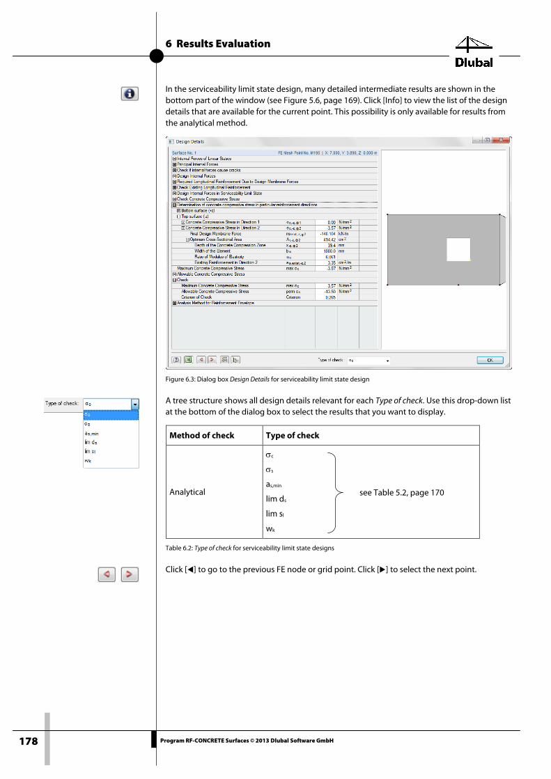
6 Results Evaluation
178 Program RF-CONCRETE Surfaces © 2013 Dlubal Software GmbH
In the serviceability limit state design, many detailed intermediate results are shown in the bottom part of the window (see Figure 5.6, page 169). Click [Info] to view the list of the design details that are available for the current point. This possibility is only available for results from the analytical method.
Figure 6.3: Dialog box Design Details for serviceability limit state design
A tree structure shows all design details relevant for each Type of check. Use this drop-down list at the bottom of the dialog box to select the results that you want to display.
Method of check Type of check
Analytical
σc
σs
as,min
lim ds
lim sl
wk
Table 6.2: Type of check for serviceability limit state designs
Click [] to go to the previous FE node or grid point. Click [] to select the next point.
see Table 5.2, page 170

6 Results Evaluation
179 Program RF-CONCRETE Surfaces © 2013 Dlubal Software GmbH
Reinforcement direction
6.2 Results on the RFEM Model To evaluate results, you can also use the RFEM work window.
RFEM background graphic and view mode The RFEM work window in the background helps you find the location of an FE node or grid point in the model. An arrow in the RFEM background graphic indicates the point selected in the results window of RF-CONCRETE Surfaces; the surface is highlighted in the selection color.
Figure 6.4: Highlighted surface and current FE node in the RFEM model
If you cannot improve the view by moving the RF-CONCRETE Surfaces module window, click [Jump to graphic to change view] to activate the View Mode: Now, the module window is hid-den so that you can adjust the view in the RFEM work window. The view mode provides only the functions of the View menu, for example zooming, moving, or rotating the display. The ar-row remains visible.
To return to RF-CONCRETE Surfaces, click [Back].
RFEM work window You can also graphically check the reinforcements and design ratios in the RFEM model. Click [Graphic] to exit the design module. The work window of RFEM now shows all design results like the internal forces of a load case.
Results navigator
The Results navigator is adjusted to the RF-CONCRETE Surfaces add-on module: It allows you to graphically show the results of the longitudinal reinforcements for each reinforcement direc-tion and layer, shear reinforcement, the design internal forces or the ratios, and detail results of the serviceability limit state designs.
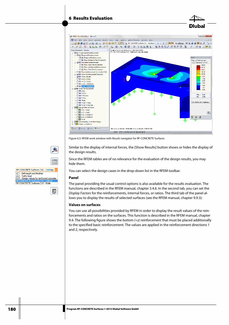
6 Results Evaluation
180 Program RF-CONCRETE Surfaces © 2013 Dlubal Software GmbH
Figure 6.5: RFEM work window with Results navigator for RF-CONCRETE Surfaces
Similar to the display of internal forces, the [Show Results] button shows or hides the display of the design results.
Since the RFEM tables are of no relevance for the evaluation of the design results, you may hide them.
You can select the design cases in the drop-down list in the RFEM toolbar.
Panel
The panel providing the usual control options is also available for the results evaluation. The functions are described in the RFEM manual, chapter 3.4.6. In the second tab, you can set the Display Factors for the reinforcements, internal forces, or ratios. The third tab of the panel al-lows you to display the results of selected surfaces (see the RFEM manual, chapter 9.9.3):
Values on surfaces
You can use all possibilities provided by RFEM in order to display the result values of the rein-forcements and ratios on the surfaces. This function is described in the RFEM manual, chapter 9.4. The following figure shows the bottom (+z) reinforcement that must be placed additionally to the specified basic reinforcement. The values are applied in the reinforcement directions 1 and 2, respectively.

6 Results Evaluation
181 Program RF-CONCRETE Surfaces © 2013 Dlubal Software GmbH
Figure 6.6: Group bottom (+z) reinforcement for required additional reinforcement
The graphics of the design results can be transferred to the printout report (see chapter 7.2, page 188).
To return to the add-on module click [RF-CONCRETE Surfaces].

6 Results Evaluation
182 Program RF-CONCRETE Surfaces © 2013 Dlubal Software GmbH
6.3 Filter for Results The results windows of RF-CONCRETE Surfaces allow you to filter the results by various criteria. In addition, the module provides filter options to evaluate the design results graphically. These options are described in the RFEM manual, chapter 9.9.
For RF-CONCRETE Surfaces, you can also use the Visibilities (see RFEM manual, chapter 9.9.1) to filter the surfaces for the evaluation.
Likewise, you can use the Sections in the RFEM model or create new ones (see RFEM manual, chapter 9.6.1). This option allows you to evaluate the results more specifically. You can redis-tribute the reinforcement peaks that stem from singularities by using the smoothing function.
Find point The results windows 2.2 and 2.3 (reinforcement) as well as 3.2 and 3.3 (serviceability) provide a search function for FE nodes and grid points. Click the button shown on the left (see Figure 6.1, page 176) to open the following dialog box.
Figure 6.7: Dialog box Find Grid Point
First, enter the number of the surface manually or click [] to select it graphically. Then, you can enter the number of the grid point or FE node, or select it in the list.
After clicking [OK], the current results window shows you the results row of this point.
Sort results By default, window 3.1 and 3.2 show the results arranged by to the maximum design ratios: The sorting conforms to table column J.
You can also sort the results by existing values from column G. The greatest ratio of the defor-mation, for example, does not necessarily represent the maximum deformation because the limit values can be defined differently for each surface. Click the [Sort Results] button to switch between these two types of result arrangement.
Filter points The button shown on the left is available in the results windows 2.2 and 2.3 (reinforcement) as well as 3.2 and 3.3 (serviceability). By clicking it, you open the following dialog box.
Figure 6.8: Dialog box Filter Points
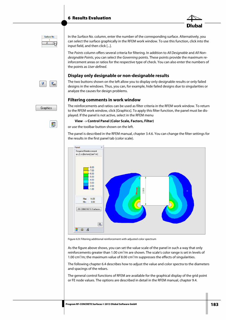
6 Results Evaluation
183 Program RF-CONCRETE Surfaces © 2013 Dlubal Software GmbH
In the Surface No. column, enter the number of the corresponding surface. Alternatively, you can select the surface graphically in the RFEM work window. To use this function, click into the input field, and then click [...].
The Points column offers several criteria for filtering. In addition to All Designable and All Non-designable Points, you can select the Governing points. These points provide the maximum re-inforcement areas or ratios for the respective type of check. You can also enter the numbers of the points as User-defined.
Display only designable or non-designable results The two buttons shown on the left allow you to display only designable results or only failed designs in the windows. Thus, you can, for example, hide failed designs due to singularities or analyze the causes for design problems.
Filtering comments in work window The reinforcements and ratios can be used as filter criteria in the RFEM work window. To return to the RFEM work window, click [Graphics]. To apply this filter function, the panel must be dis-played. If the panel is not active, select in the RFEM menu
View → Control Panel (Color Scale, Factors, Filter)
or use the toolbar button shown on the left.
The panel is described in the RFEM manual, chapter 3.4.6. You can change the filter settings for the results in the first panel tab (color scale).
Figure 6.9: Filtering additional reinforcement with adjusted color spectrum
As the figure above shows, you can set the value scale of the panel in such a way that only reinforcements greater than 1.00 cm2/m are shown. The scale's color range is set in levels of 1.00 cm2/m; the maximum value of 8.00 cm2/m suppresses the effects of singularities.
The following chapter 6.4 describes how to adjust the value and color spectra to the diameters and spacings of the rebars.
The general control functions of RFEM are available for the graphical display of the grid point or FE node values. The options are described in detail in the RFEM manual, chapter 9.4.
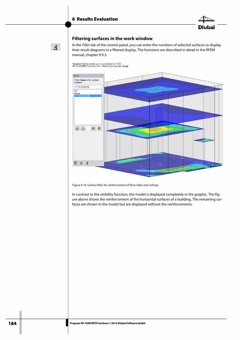
6 Results Evaluation
184 Program RF-CONCRETE Surfaces © 2013 Dlubal Software GmbH
Filtering surfaces in the work window In the Filter tab of the control panel, you can enter the numbers of selected surfaces to display their result diagrams in a filtered display. The functions are described in detail in the RFEM manual, chapter 9.9.3.
Figure 6.10: Surface filter for reinforcement of floor slabs and ceilings
In contrast to the visibility function, the model is displayed completely in the graphic. The fig-ure above shows the reinforcement of the horizontal surfaces of a building. The remaining sur-faces are shown in the model but are displayed without the reinforcements.

6 Results Evaluation
185 Program RF-CONCRETE Surfaces © 2013 Dlubal Software GmbH
6.4 Configuring the Panel The reinforcement results can be shown graphically as isobands or isolines. Twelve color zones are set by default for the value spectrum, covering a range between minimum and maximum value. You can also adjust the value spectrum regarding the definition of the reinforcement in order to prepare the graphical results for a reinforcement drawing.
To adjust the panel, double click one of the colors. You can also use the [Options] button avail-able in the panel: The Options dialog box opens, where you can click the [Edit] button to access another dialog box for changing the ranges of colors and values.
In the Edit Isoband Value and Color Spectra dialog box, you can click [Edit] to open the Edit Value Spectrum with Reinforcement Definition dialog box.
Figure 6.11: Dialog boxes Edit Isoband Value and Color Spectra and Edit Value Spectrum with Reinforcement Definition
This dialog box determines the reinforcement area per meter from the Diameter and the Dis-tance of the rebars. In the Additional Rebars columns, you can assign further rebar diameters and distances (see Figure 6.12). Thus, you can set user-defined value spectra for the reinforce-ment, which can only be used for the reinforcement drawing.
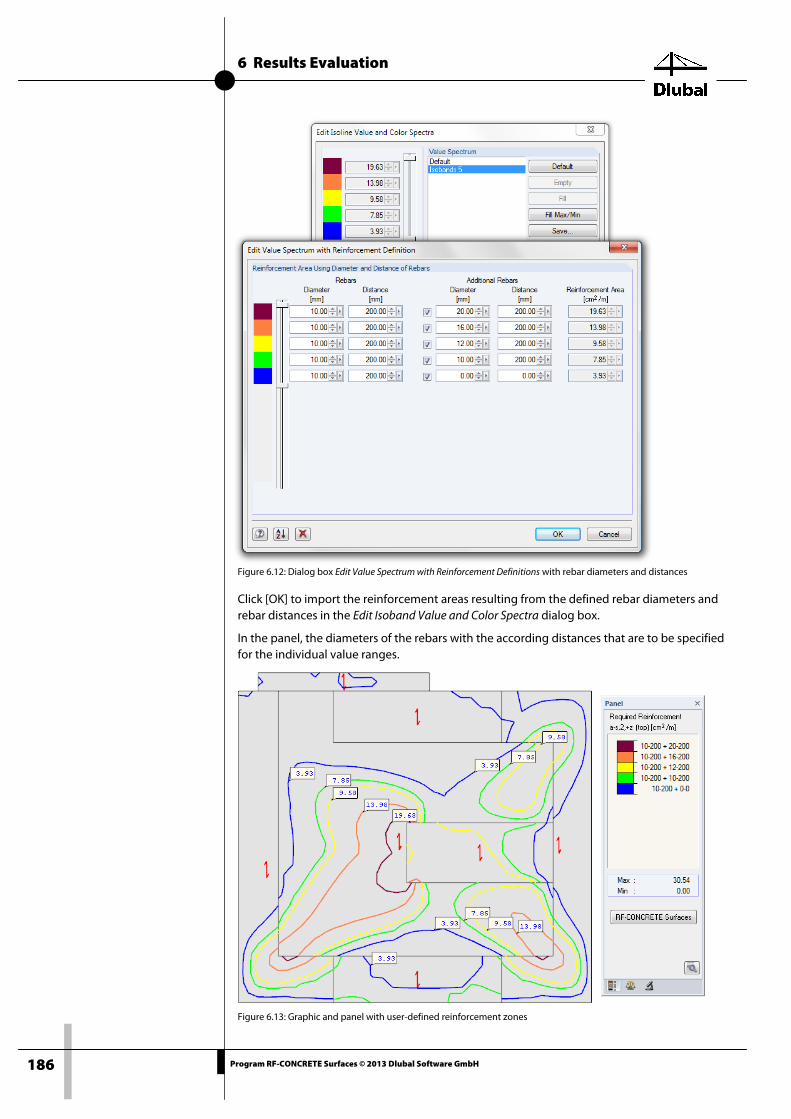
6 Results Evaluation
186 Program RF-CONCRETE Surfaces © 2013 Dlubal Software GmbH
Figure 6.12: Dialog box Edit Value Spectrum with Reinforcement Definitions with rebar diameters and distances
Click [OK] to import the reinforcement areas resulting from the defined rebar diameters and rebar distances in the Edit Isoband Value and Color Spectra dialog box.
In the panel, the diameters of the rebars with the according distances that are to be specified for the individual value ranges.
Figure 6.13: Graphic and panel with user-defined reinforcement zones

7 Printout
187 Program RF-CONCRETE Surfaces © 2013 Dlubal Software GmbH
7. Printout
7.1 Printout Report The creation of printouts for the data of RF-CONCRETE Surfaces is similar to the procedure in RFEM: The program generates a printout report for the RF-CONCRETE Surfaces results; graphics and descriptions can be added subsequently. The selection in the printout report controls the design module data that will finally appear in the printout.
The printout report is described in the RFEM manual. Chapter 10.1.3.4 Selecting Data of Add-on Modules describes how the input and output data can be prepared for the printout.
A special selection option is available for the intermediate results of serviceability limit state designs according to the analytical method. In the Points column, you can select all designable, all non-designable, or only the Governing points: These points provide the greatest reinforce-ment areas or ratios. You can also enter User-defined point numbers.
Figure 7.1: Dialog box Printout Report Selection, tab SLS - Analytical Method
For complex structural systems with a high number of design cases, it is recommended to split the data into several printout reports to make data arrangement clearer.
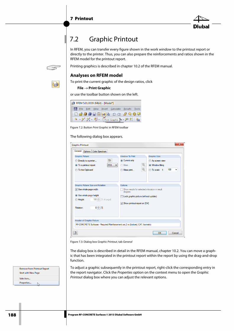
7 Printout
188 Program RF-CONCRETE Surfaces © 2013 Dlubal Software GmbH
7.2 Graphic Printout In RFEM, you can transfer every figure shown in the work window to the printout report or directly to the printer. Thus, you can also prepare the reinforcements and ratios shown in the RFEM model for the printout report.
Printing graphics is described in chapter 10.2 of the RFEM manual.
Analyses on RFEM model To print the current graphic of the design ratios, click
File → Print Graphic
or use the toolbar button shown on the left.
Figure 7.2: Button Print Graphic in RFEM toolbar
The following dialog box appears.
Figure 7.3: Dialog box Graphic Printout, tab General
The dialog box is described in detail in the RFEM manual, chapter 10.2. You can move a graph-ic that has been integrated in the printout report within the report by using the drag-and-drop function.
To adjust a graphic subsequently in the printout report, right-click the corresponding entry in the report navigator. Click the Properties option on the context menu to open the Graphic Printout dialog box where you can adjust the relevant options.
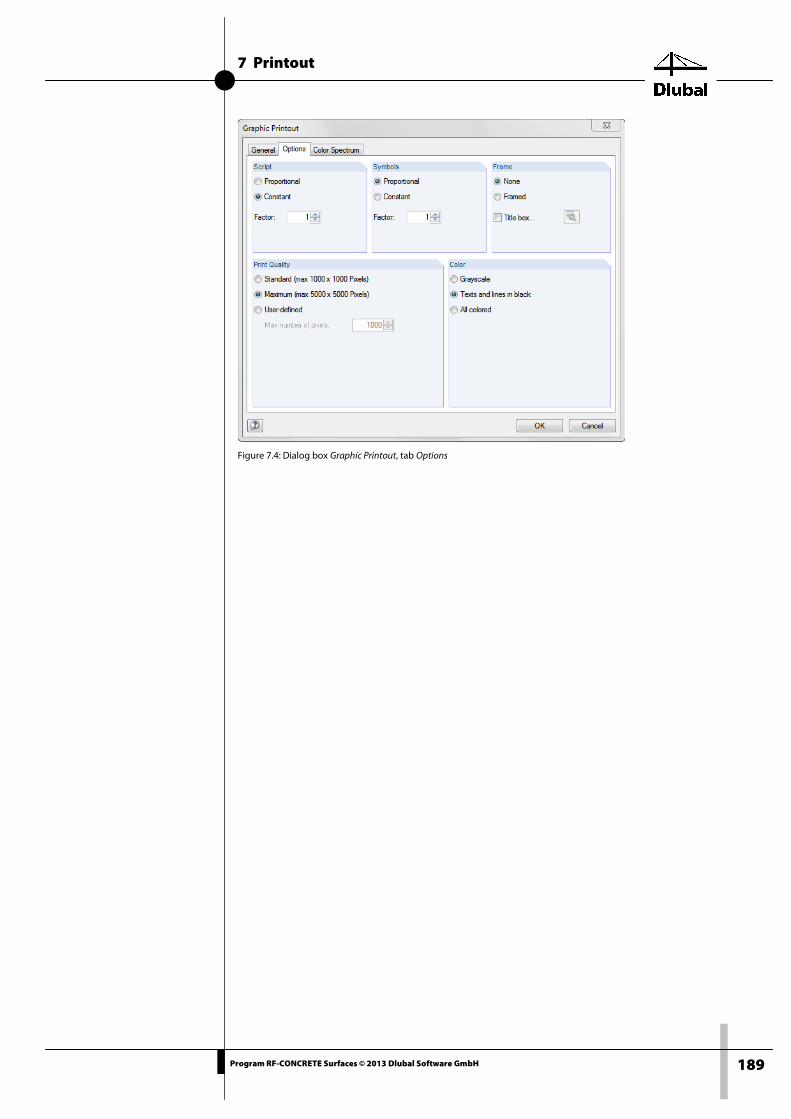
7 Printout
189 Program RF-CONCRETE Surfaces © 2013 Dlubal Software GmbH
Figure 7.4: Dialog box Graphic Printout, tab Options

8 General Functions
190 Program RF-CONCRETE Surfaces © 2013 Dlubal Software GmbH
8. General Functions This chapter describes some useful menu functions as well as export options for the designs.
8.1 Design Cases Design cases allow you to group surfaces for the designs or to design different variants (for ex-ample, modified materials of reinforcement specifications, nonlinear analysis).
It is no problem to analyze a surface in different design cases.
The design cases of RF-CONCRETE Surfaces can also be selected in RFEM by using the load case list in the toolbar.
Creating new design case To create a new design case in RF-CONCRETE Surfaces, click
File → New Case.
The following dialog box appears:
Figure 8.1: Dialog box New RF-CONCRETE Surfaces Case
In this dialog box, you enter a No. (one that is not yet assigned) for the new design case. A Description will make the selection in the load case list easier.
After you click [OK], the 1.1 General Data window opens where you can enter the new design data.
Renaming design case To change the description of a design case, click
File → Rename Case.
The following dialog box appears:
Figure 8.2: Dialog box Rename RF-CONCRETE Surfaces Case
Here, you can specify a different Description but also a different No. for the design case.
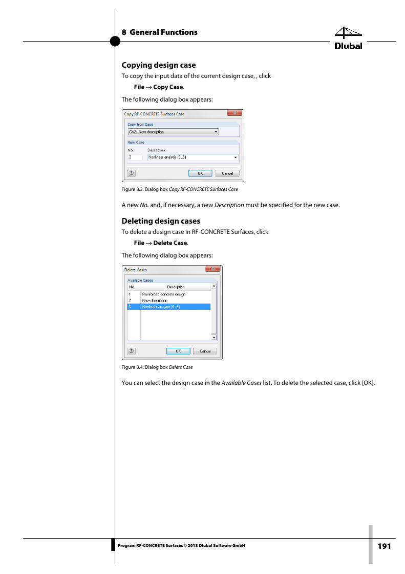
8 General Functions
191 Program RF-CONCRETE Surfaces © 2013 Dlubal Software GmbH
Copying design case To copy the input data of the current design case, , click
File → Copy Case.
The following dialog box appears:
Figure 8.3: Dialog box Copy RF-CONCRETE Surfaces Case
A new No. and, if necessary, a new Description must be specified for the new case.
Deleting design cases To delete a design case in RF-CONCRETE Surfaces, click
File → Delete Case.
The following dialog box appears:
Figure 8.4: Dialog box Delete Case
You can select the design case in the Available Cases list. To delete the selected case, click [OK].

8 General Functions
192 Program RF-CONCRETE Surfaces © 2013 Dlubal Software GmbH
8.2 Units and Decimal Places The units and decimal places for RFEM and the add-on modules are managed in one dialog box. In the RF-CONCRETE Surfaces add-on module, you can open the dialog box to define the units by clicking
Settings → Units and Decimal Places.
The dialog box known from RFEM appears. RF-CONCRETE Surfaces is preset in the Program /
Module list.
Figure 8.5: Dialog box Units and Decimal Places
The settings can be saved as user profile to reuse them in other models. These functions are described in the RFEM manual, chapter 11.1.3.

8 General Functions
193 Program RF-CONCRETE Surfaces © 2013 Dlubal Software GmbH
8.3 Export of Results The results of RF-CONCRETE Surfaces can also be used in other programs.
Clipboard To copy cells selected in the results windows of RF-CONCRETE Surfaces to the Clipboard, press [Ctrl]+[C]. To insert the cells, for example in a word processing program, press [Ctrl]+[V]. The headers of the table columns are not transferred.
Printout Report The data of RF-CONCRETE Surfaces can be printed into the global printout report (see chapter 7.1, page 187), and then exported. In the printout report, click
File → Export in RTF.
The function is described in the RFEM manual, chapter 10.1.11.
Excel / OpenOffice The module RF-CONCRETE Surfaces provides a function for the direct data export to MS Excel, OpenOffice.org Calc, or in the CSV format. To open the corresponding dialog box, click
File → Export Tables.
The following export dialog box appears.
Figure 8.6: Dialog box Export - MS Excel
If your selection is complete, click [OK] to start the export. Excel or OpenOffice are started automatically, that is, you do not need to open the programs first.

8 General Functions
194 Program RF-CONCRETE Surfaces © 2013 Dlubal Software GmbH
Figure 8.7: Results in Excel
CAD programs
The reinforcement areas determined in RF-CONCRETE Surfaces can also be used in CAD pro-grams. RFEM provides interfaces to the following programs:
• Nemetschek (FEM format for Allplan *.asf)
• Glaser (Format *.fem)
• Strakon (Format *.cfe)
To use this export function in RFEM, click
File → Export.
The Export dialog box appears where you can select the relevant interface. The dialog box is described in detail in the RFEM manual, chapter 12.5.2
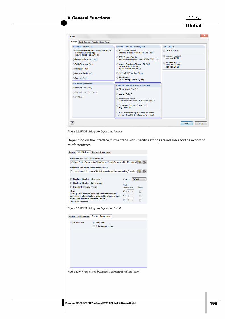
8 General Functions
195 Program RF-CONCRETE Surfaces © 2013 Dlubal Software GmbH
Figure 8.8: RFEM dialog box Export, tab Format
Depending on the interface, further tabs with specific settings are available for the export of reinforcements.
Figure 8.9: RFEM dialog box Export, tab Details
Figure 8.10: RFEM dialog box Export, tab Results - Glaser (.fem)
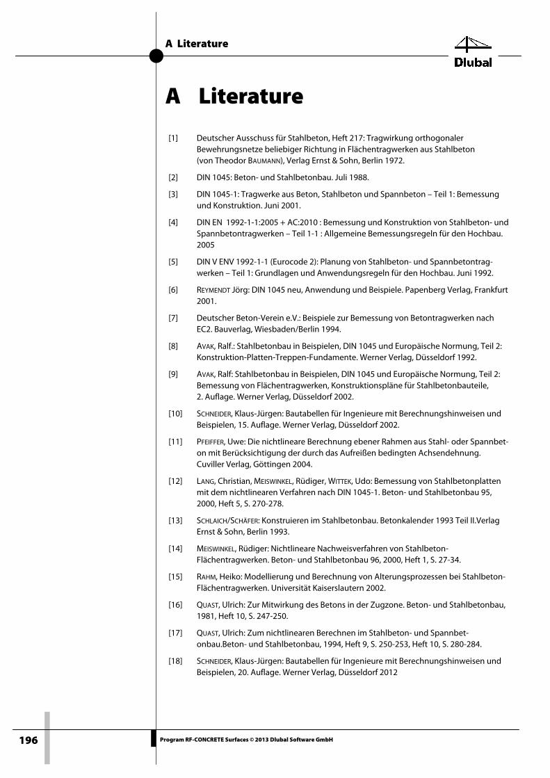
A Literature
196 Program RF-CONCRETE Surfaces © 2013 Dlubal Software GmbH
A Literature
[1] Deutscher Ausschuss für Stahlbeton, Heft 217: Tragwirkung orthogonaler Bewehrungsnetze beliebiger Richtung in Flächentragwerken aus Stahlbeton (von Theodor BAUMANN), Verlag Ernst & Sohn, Berlin 1972.
[2] DIN 1045: Beton- und Stahlbetonbau. Juli 1988.
[3] DIN 1045-1: Tragwerke aus Beton, Stahlbeton und Spannbeton – Teil 1: Bemessung und Konstruktion. Juni 2001.
[4] DIN EN 1992-1-1:2005 + AC:2010 : Bemessung und Konstruktion von Stahlbeton- und Spannbetontragwerken – Teil 1-1 : Allgemeine Bemessungsregeln für den Hochbau. 2005
[5] DIN V ENV 1992-1-1 (Eurocode 2): Planung von Stahlbeton- und Spannbetontrag-werken – Teil 1: Grundlagen und Anwendungsregeln für den Hochbau. Juni 1992.
[6] REYMENDT Jörg: DIN 1045 neu, Anwendung und Beispiele. Papenberg Verlag, Frankfurt 2001.
[7] Deutscher Beton-Verein e.V.: Beispiele zur Bemessung von Betontragwerken nach EC2. Bauverlag, Wiesbaden/Berlin 1994.
[8] AVAK, Ralf.: Stahlbetonbau in Beispielen, DIN 1045 und Europäische Normung, Teil 2: Konstruktion-Platten-Treppen-Fundamente. Werner Verlag, Düsseldorf 1992.
[9] AVAK, Ralf: Stahlbetonbau in Beispielen, DIN 1045 und Europäische Normung, Teil 2: Bemessung von Flächentragwerken, Konstruktionspläne für Stahlbetonbauteile, 2. Auflage. Werner Verlag, Düsseldorf 2002.
[10] SCHNEIDER, Klaus-Jürgen: Bautabellen für Ingenieure mit Berechnungshinweisen und Beispielen, 15. Auflage. Werner Verlag, Düsseldorf 2002.
[11] PFEIFFER, Uwe: Die nichtlineare Berechnung ebener Rahmen aus Stahl- oder Spannbet-on mit Berücksichtigung der durch das Aufreißen bedingten Achsendehnung. Cuviller Verlag, Göttingen 2004.
[12] LANG, Christian, MEISWINKEL, Rüdiger, WITTEK, Udo: Bemessung von Stahlbetonplatten mit dem nichtlinearen Verfahren nach DIN 1045-1. Beton- und Stahlbetonbau 95, 2000, Heft 5, S. 270-278.
[13] SCHLAICH/SCHÄFER: Konstruieren im Stahlbetonbau. Betonkalender 1993 Teil II.Verlag Ernst & Sohn, Berlin 1993.
[14] MEISWINKEL, Rüdiger: Nichtlineare Nachweisverfahren von Stahlbeton-Flächentragwerken. Beton- und Stahlbetonbau 96, 2000, Heft 1, S. 27-34.
[15] RAHM, Heiko: Modellierung und Berechnung von Alterungsprozessen bei Stahlbeton-Flächentragwerken. Universität Kaiserslautern 2002.
[16] QUAST, Ulrich: Zur Mitwirkung des Betons in der Zugzone. Beton- und Stahlbetonbau, 1981, Heft 10, S. 247-250.
[17] QUAST, Ulrich: Zum nichtlinearen Berechnen im Stahlbeton- und Spannbet-onbau.Beton- und Stahlbetonbau, 1994, Heft 9, S. 250-253, Heft 10, S. 280-284.
[18] SCHNEIDER, Klaus-Jürgen: Bautabellen für Ingenieure mit Berechnungshinweisen und Beispielen, 20. Auflage. Werner Verlag, Düsseldorf 2012
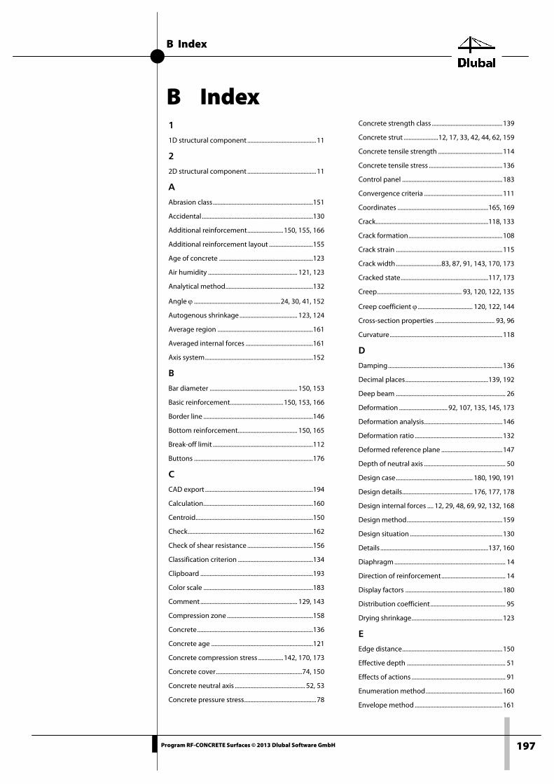
B Index
197 Program RF-CONCRETE Surfaces © 2013 Dlubal Software GmbH
B Index 1 1D structural component ............................................ 11
2 2D structural component ............................................ 11
A Abrasion class ................................................................151
Accidental .......................................................................130
Additional reinforcement ....................... 150, 155, 166
Additional reinforcement layout ............................155
Age of concrete ............................................................123
Air humidity ......................................................... 121, 123
Analytical method........................................................132
Angle ϕ ....................................................... 24, 30, 41, 152
Autogenous shrinkage ..................................... 123, 124
Average region .............................................................161
Averaged internal forces ...........................................161
Axis system .....................................................................152
B Bar diameter ........................................................ 150, 153
Basic reinforcement.................................. 150, 153, 166
Border line ......................................................................146
Bottom reinforcement ...................................... 150, 165
Break-off limit ................................................................112
Buttons ............................................................................176
C CAD export .....................................................................194
Calculation ......................................................................160
Centroid ...........................................................................150
Check ................................................................................162
Check of shear resistance ..........................................156
Classification criterion ................................................134
Clipboard ........................................................................193
Color scale ......................................................................183
Comment .............................................................. 129, 143
Compression zone .......................................................158
Concrete ..........................................................................136
Concrete age .................................................................121
Concrete compression stress ................ 142, 170, 173
Concrete cover ....................................................... 74, 150
Concrete neutral axis ............................................. 52, 53
Concrete pressure stress .............................................. 78
Concrete strength class ............................................. 139
Concrete strut ...................... 12, 17, 33, 42, 44, 62, 159
Concrete tensile strength ......................................... 114
Concrete tensile stress ............................................... 136
Control panel ................................................................ 183
Convergence criteria .................................................. 111
Coordinates .......................................................... 165, 169
Crack........................................................................ 118, 133
Crack formation ............................................................ 108
Crack strain .................................................................... 115
Crack width ............................. 83, 87, 91, 143, 170, 173
Cracked state ........................................................ 117, 173
Creep ...................................................... 93, 120, 122, 135
Creep coefficient ϕ ................................... 120, 122, 144
Cross-section properties ...................................... 93, 96
Curvature ........................................................................ 118
D Damping ......................................................................... 136
Decimal places ..................................................... 139, 192
Deep beam ...................................................................... 26
Deformation ............................... 92, 107, 135, 145, 173
Deformation analysis .................................................. 146
Deformation ratio ........................................................ 132
Deformed reference plane ....................................... 147
Depth of neutral axis .................................................... 50
Design case ................................................. 180, 190, 191
Design details ............................................. 176, 177, 178
Design internal forces .... 12, 29, 48, 69, 92, 132, 168
Design method ............................................................. 159
Design situation ........................................................... 130
Details ..................................................................... 137, 160
Diaphragm ....................................................................... 14
Direction of reinforcement ......................................... 14
Display factors .............................................................. 180
Distribution coefficient ................................................ 95
Drying shrinkage .......................................................... 123
E Edge distance ................................................................ 150
Effective depth ............................................................... 51
Effects of actions ............................................................ 91
Enumeration method ................................................. 160
Envelope method ........................................................ 161

B Index
198 Program RF-CONCRETE Surfaces © 2013 Dlubal Software GmbH
Eurocode .........................................................................137
Excel ..................................................................................193
Exit RF-CONCRETE Surfaces ......................................127
Export ..................................................................... 135, 193
Exposure class ...............................................................151
F Factor kt ...........................................................................138
FE node .................... 164, 165, 168, 169, 172, 175, 182
Filter ............................................ 169, 176, 182, 183, 184
Flowchart ........................................................................132
Fundamental .................................................................130
G General data ............................................................ 10, 127
Glaser ................................................................................194
Governing points ............................................... 183, 187
Graphic ............................................................................179
Graphic printout ...........................................................188
Grid point ................ 164, 165, 168, 169, 172, 175, 182
I
Inclination of concrete strut θ ........................... 42, 158
Installation .......................................................................... 8
Intermediate results .......................................... 169, 173
Internal forces ............................................... 91, 107, 163
Iteration method ..........................................................110
Iterations .........................................................................136
L Layer ....................................................................... 107, 136
Lever arm ............................................................ 49, 53, 54
Limit state of serviceability ............................. 141, 169
Limit values ....................................................................128
Limitation of rebar diameter ....................................170
Load case .............................................. 91, 130, 131, 170
Load combination .............................................. 130, 138
Load duration factor ...................................................137
Load situation .................................................................. 21
Longitudinal reinforcement ...... 36, 39, 63, 133, 153, 156, 165
Long-term effects .................................................. 93, 158
M Material .................................................................. 136, 138
Material description ....................................................139
Material library ..............................................................140
Material properties ......................................................139
Maximum bar diameter ........................................ 81, 84
Maximum reinforcement .......................................... 149
Mesh reinforcement ................................................... 154
Method ............................................................................ 132
Method of check ................................................. 131, 144
Minimum reinforcement ........ 25, 26, 27, 66, 81, 149, 157, 170
Mixed method .............................................................. 161
Module windows ......................................................... 127
Modulus of elasticity ................................................... 121
Most economical reinforcement ............................ 133
N National Annex ............................................................. 128
Navigator ........................................................................ 127
Nemetschek ................................................................... 194
Neutral axis depth ....................................................... 158
Non-designable ......................................... 166, 170, 176
Nonlinear method ........................... 107, 134, 144, 173
Nonlinear stiffness ....................................................... 135
Note .................................................................................. 143
O OpenOffice ..................................................................... 193
Optimization ................................................................. 159
Options ............................................................................ 135
Orthotropic ........................................................... 142, 144
P Panel.......................................................... 9, 180, 183, 185
Parallel surface .............................................................. 146
Partial safety factor for concrete ............................. 158
Partial safety factor for reinforcing steel .............. 158
Permanent load ............................................................ 138
Plate ............................. 10, 25, 28, 66, 71, 132, 145, 157
Plausibility check ......................................................... 162
Point coordinates ............................................... 165, 169
Principal axial force ....................................................... 21
Print ......................................................................... 176, 188
Printout report ..................................................... 187, 188
Provided reinforcement .............................................. 74
R Ratio ................................................................................. 170
Rebar ....................................................................... 154, 185
Rebar diameter .................................................... 155, 185
Rebar distance .............................................. 86, 170, 185
Reduction factor α ....................................................... 158
Reduction parameter VMB .............................. 116, 118
Reference plane ........................................................... 147

B Index
199 Program RF-CONCRETE Surfaces © 2013 Dlubal Software GmbH
Reference scale .............................................................176
Reinforcement......................... 148, 164, 165, 166, 167
Reinforcement area .....................................................153
Reinforcement direction .................................. 149, 152
Reinforcement envelope ...........................................160
Reinforcement group .................................................148
Reinforcement layout .................................................149
Reinforcement ratio ....................................................149
Reinforcing steel ................................................. 136, 139
Reinforcing steel stress..................... 80, 142, 170, 173
Required reinforcement.............................................155
Restraint ..........................................................................143
Result combination 91, 130, 131, 134, 138, 160, 170
Results evaluation ........................................................176
Results graphic ..............................................................179
Results navigator ..........................................................179
Results values in graphic ...........................................180
Results windows ...........................................................164
RF-CONCRETE Deflect ................................ 92, 133, 141
RF-CONCRETE NL .............................. 107, 124, 134, 144
RFEM graphic .................................................................188
RFEM work window .....................................................179
Rib .....................................................................................162
S Search function .............................................................182
Secondary reinforcement ..........................................149
Section .............................................................................182
Selecting module windows ......................................127
Selection printout ........................................................187
Serviceability limit state 69, 107, 119, 131, 141, 155, 166, 169, 170, 173, 178
Shear design ............................................................. 37, 64
Shear reinforcement ......................................... 158, 165
Shear resistance ......................................... 37, 42, 44, 65
Shell ............................................................................. 25, 48
Shrinkage ........................... 93, 123, 124, 126, 135, 145
Shrinkage strain ............................................................123
Singularity ................................................... 161, 182, 183
Sorting .................................................................... 176, 182
Standard ........................................................... 6, 128, 157
Start calculation ........................................................... 163
Start program ..................................................................... 8
Start RF-CONCRETE Surfaces ......................................... 8
State II ..................................................................... 117, 173
Stiffness ........................................................................... 135
Strain ................................................................ 89, 107, 122
Strakon ............................................................................ 194
Stresses ................................................................... 133, 135
Stress-strain relationship ........................ 113, 118, 136
Structural system ......................................................... 124
Surface .............................. 141, 148, 152, 167, 171, 174
Symbol ......................................................... 165, 168, 170
T Tensile strength of concrete .................................... 143
Tension stiffening ........................................ 95, 115, 136
Thickness ........................................................................ 142
Top reinforcement ............................................. 150, 165
Type of cement .................................................... 122, 123
Type of check ....................................................... 173, 178
Type of model ................................................................. 10
U Ultimate limit state ................... 37, 130, 165, 166, 177
Undeformed system ................................................... 146
Units ........................................................................ 139, 192
User profile ..................................................................... 192
V Value spectrum ............................................................. 185
View mode ............................................................ 176, 179
Visibilities ........................................................................ 182
W Wall ....... 10, 14, 20, 25, 26, 66, 71, 132, 151, 158, 159
Y Yielding ........................................................................... 115