Report EUR 27351 EN

Francesco Di Comite

Olga Diukanova

d’Artis Kancs

A Dynamic Spatial General

Equilibrium Model for EU

Regions and Sectors

RHOMOLO Model Manual

2015

European Commission

Joint Research Centre

Institute for Prospective Technological Studies

Contact information

d’Artis Kancs

Address: Edificio Expo. c/ Inca Garcilaso, 3. E-41092 Seville (Spain)

E-mail: d’artis.kancs@ec.europa.eu

Tel.: +34 954488318

Fax: +34 954488300

JRC Science Hub

https://ec.europa.eu/jrc

Legal Notice

This publication is a Technical Report by the Joint Research Centre, the European Commission’s in-house science service.

It aims to provide evidence-based scientific support to the European policy-making process. The scientific output expressed does not

imply a policy position of the European Commission. Neither the European Commission nor any person acting on behalf of the

Commission is responsible for the use which might be made of this publication.

All images © European Union 2015

JRC96776

EUR 27351 EN

ISBN 978-92-79-49579-3 (PDF)

ISSN 1831-9424 (online)

doi:10.2791/185683

Luxembourg: Publications Office of the European Union, 2015

© European Union, 2015

Reproduction is authorised provided the source is acknowledged.

Abstract

This manual explains how to practically use the Regional Holistic Model (RHOMOLO) for policy impact assessment. RHOMOLO is the

dynamic spatial general equilibrium model of the European Commission. It is developed by DG JRC for policy impact assessment and

provides sector-, region- and time-specific support to EU policy makers on structural reforms, growth and regional policies. The

current version of RHOMOLO covers all NUTS2 regions of the EU, and each regional economy is disaggregated into six economic

sectors. Spatial interactions between regions are captured through trade of goods and services (which is subject to trade costs), factor

mobility and knowledge spillovers, making RHOMOLO particularly well suited for simulating human capital, transport infrastructure,

R&D and innovation policies. In this manual we explain the logic of its modular structure and provide a step-by step guide to perform

simulations using either its GAMS-IDE interface or a user-friendly graphical web interface.

JEL codes: C63, C68, D58, F12, H41, O31, O40, R13, R30, R40.

Keywords: Spatial computable general equilibrium, economic modelling, spatial dynamics, policy impact assessment, economic

geography.

3

Contents

1 INTRODUCTION .............................................................................................................................................................................. 6

2 OVERVIEW OF THE RHOMOLO MODEL ............................................................................................................................. 8

2.1 Product markets: segmentation and differentiation ................................................................................ 8

2.2 Labour markets: unemployment and migration ......................................................................................... 9

2.3 Modelling innovation: R&D and knowledge spillovers ............................................................................. 9

2.4 New Economic Geography features ................................................................................................................ 10

2.5 Recursive dynamics and equilibria................................................................................................................... 10

2.6 Performing policy simulations with RHOMOLO ........................................................................................ 11

3 POLICY SIMULATIONS VIA THE GRAPHICAL WEB-INTERFACE.......................................................................... 11

3.1 Step 3 - Calculation of counterfactual equilibrium ................................................................................ 13

3.2 Step 4 - Policy appraisal based on comparison between the counterfactual and the baseline projections .................................................................................................................................................. 14

4 POLICY SIMULATIONS VIA THE GAMS-IDE INTERFACE ........................................................................................ 18

4.1 RHOMOLO setup in the GAMS-IDE ................................................................................................................... 18

4.2 RHOMOLO file organisation ................................................................................................................................. 20

4.3 Running policy simulations with RHOMOLO in GAMS-IDE.................................................................. 29

4.3.1 Step 1 - Compilation of micro-consistent base year data .......................................... 29

4.3.2 Step 2 – Calibration of the model .............................................................................................. 29

4.3.3 Step 3 - Calculation of counterfactual equilibrium .......................................................... 30

4.3.4 Step 4 - Policy appraisal based on comparison between the counterfactual and the baseline projections ........................................................................ 30

4.3.5 Step 5 - Sensitivity analysis .......................................................................................................... 34

4

5 CONCLUDING REMARKS......................................................................................................................................................... 38

6 REFERENCES ................................................................................................................................................................................. 39

7 APPENDICES ................................................................................................................................................................................. 41

7.1 Appendix 1. Content of the batch script RunAllSCN.cmd to run sensitivity analysis for different combinations of model elasticity parameters ..................................................................... 41

7.2 Appendix 2. Content of file RunRhomolo_SSA.gms that loops over all possible values of elasticity parameters, allocates model runs to 24 parallel processes on 24 CPU and merges results into Excel Pivot tables ................................................................................................. 42

7.3 Appendix 3. Content of the “model interface file” RunRhomolo_SSA.gms adjusted for running sensitivity analysis .......................................................................................................................... 45

5

RHOMOLO Model Manual

A Dynamic Spatial General Equilibrium Model for EU Regions and Sectors

Francesco Di Comite, Olga Diukanova and d'Artis Kancs1

European Commission, DG Joint Research Centre, Seville (Spain)

Abstract: This manual explains how to practically use European Commission's dynamic spatial general

equilibrium model RHOMOLO (Regional Holistic Model) for policy impact assessment. The model is developed by the Joint Research Centre (DG JRC) to provide sector-, region- and time-specific support to EU policy makers on structural reforms, growth and regional policies. The current version of RHOMOLO covers all NUTS2 regions of the EU, each regional economy being disaggregated into six economic sectors. Spatial interactions between regions are captured by trade matrices for goods and services, factor mobility and knowledge spillovers, making RHOMOLO particularly well suited for simulating human capital, transport infrastructure, R&D and innovation policies. Recently, the RHOMOLO model has been used together with the Directorate-General for Regional and Urban Policy (DG REGIO) for impact assessment of Cohesion Policy, and with the European Investment Bank for impact assessment of EU investment support policies. In this manual we explain the logic of its modular structure and provide a

step-by step guide to perform simulations using either its GAMS-IDE interface or a user-friendly graphical web interface.

JEL classification: C68, D58, F12, O31, R13.

Keywords: Spatial computable general equilibrium, economic modelling, spatial dynamics, policy impact

assessment, economic geography.

1The views expressed are purely those of the authors and may not in any circumstances be regarded as stating an official position of the European Commission. The authors are grateful to Damiaan Persyn and Sergio Romero Villa for their valuable contributions to the RHOMOLO web interface.

6

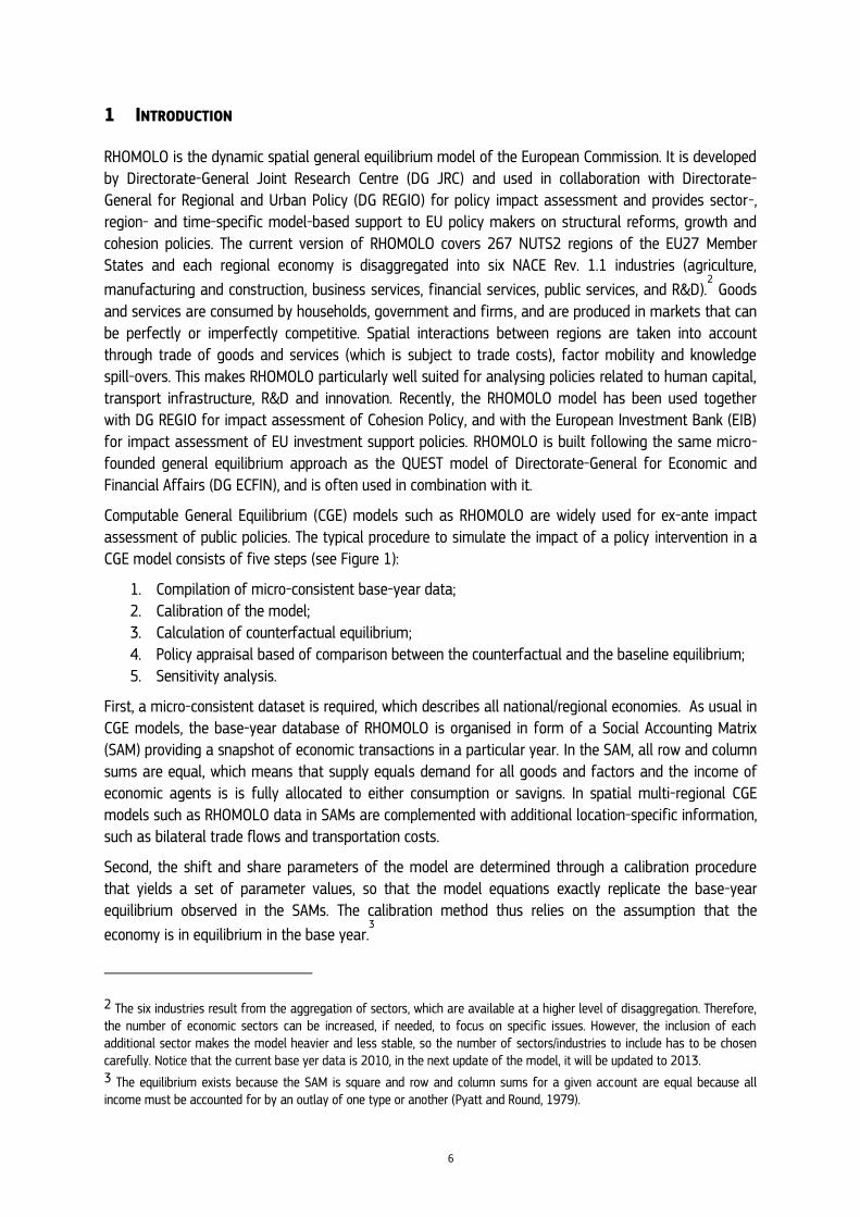
1 INTRODUCTION

RHOMOLO is the dynamic spatial general equilibrium model of the European Commission. It is developed by Directorate-General Joint Research Centre (DG JRC) and used in collaboration with Directorate-General for Regional and Urban Policy (DG REGIO) for policy impact assessment and provides sector-, region- and time-specific model-based support to EU policy makers on structural reforms, growth and cohesion policies. The current version of RHOMOLO covers 267 NUTS2 regions of the EU27 Member States and each regional economy is disaggregated into six NACE Rev. 1.1 industries (agriculture,

manufacturing and construction, business services, financial services, public services, and R&D).2 Goods

and services are consumed by households, government and firms, and are produced in markets that can

be perfectly or imperfectly competitive. Spatial interactions between regions are taken into account through trade of goods and services (which is subject to trade costs), factor mobility and knowledge spill-overs. This makes RHOMOLO particularly well suited for analysing policies related to human capital, transport infrastructure, R&D and innovation. Recently, the RHOMOLO model has been used together with DG REGIO for impact assessment of Cohesion Policy, and with the European Investment Bank (EIB) for impact assessment of EU investment support policies. RHOMOLO is built following the same micro-founded general equilibrium approach as the QUEST model of Directorate-General for Economic and Financial Affairs (DG ECFIN), and is often used in combination with it.

Computable General Equilibrium (CGE) models such as RHOMOLO are widely used for ex-ante impact assessment of public policies. The typical procedure to simulate the impact of a policy intervention in a

CGE model consists of five steps (see Figure 1):

1. Compilation of micro-consistent base-year data; 2. Calibration of the model; 3. Calculation of counterfactual equilibrium; 4. Policy appraisal based of comparison between the counterfactual and the baseline equilibrium; 5. Sensitivity analysis.

First, a micro-consistent dataset is required, which describes all national/regional economies. As usual in CGE models, the base-year database of RHOMOLO is organised in form of a Social Accounting Matrix

(SAM) providing a snapshot of economic transactions in a particular year. In the SAM, all row and column

sums are equal, which means that supply equals demand for all goods and factors and the income of economic agents is is fully allocated to either consumption or savigns. In spatial multi-regional CGE models such as RHOMOLO data in SAMs are complemented with additional location-specific information, such as bilateral trade flows and transportation costs.

Second, the shift and share parameters of the model are determined through a calibration procedure that yields a set of parameter values, so that the model equations exactly replicate the base-year equilibrium observed in the SAMs. The calibration method thus relies on the assumption that the

economy is in equilibrium in the base year.3

2 The six industries result from the aggregation of sectors, which are available at a higher level of disaggregation. Therefore, the number of economic sectors can be increased, if needed, to focus on specific issues. However, the inclusion of each additional sector makes the model heavier and less stable, so the number of sectors/industries to include has to be chosen carefully. Notice that the current base yer data is 2010, in the next update of the model, it will be updated to 2013. 3 The equilibrium exists because the SAM is square and row and column sums for a given account are equal because all income must be accounted for by an outlay of one type or another (Pyatt and Round, 1979).

7

Third, policy simulations are undertaken by altering some parameters or variables of the model (in CGE jargon this is referred to as a policy "shock" to the model). The examples of policies that can be simulated with RHOMOLO include R&D and innovation, investment in human capital, investment in transport infrastructure, structural reforms, subsidies to firms / industries and tax reforms, among others. For any policy impact assessment, or counterfactual experiment, the same calibrated parameter values as in the benchmark are used to solve for the associated equilibria after a policy shock.

Fourth, the effects of the policy experiment are evaluated by comparing the benchmark and the counterfactual equilibria. Usually, the results are calculated and presented as percentage deviations from the benchmark.

In a final step, sensitivity analysis with respect to the key assumptions and parameter values in the model are carried out to test the robustness of the results to alternative modelling choices, such as the values of behavioural parameters (elasticities), functional forms, etc.

Figure 1: Main steps in CGE modelling. Source: Shoven and Whalley (1992).

The rest of the manual describes how to practically use the RHOMOLO model to carry out policy

simulations along these five CGE modelling steps. Section 2 provides a brief overview of the RHOMOLO model. In Section 3 we show how to use the web interface to perform simulations with RHOMOLO. Section 4 explains how to use GAMS-IDE interface to carry out policy simulations and how RHOMOLO file structure is organised, including the reporting of policy simulation results. Section 5 offers some concluding remarks comparing the advantages and disadvantages of each approach.

8

2 OVERVIEW OF THE RHOMOLO MODEL

In the tradition of Computable General Equilibrium (CGE) models, RHOMOLO relies on a general equilibrium framework à la Arrow-Debreu where supply and demand are influenced by a system of prices subject to macroeconomic constraints.4 Policies are introduced as shocks to the existing equilibrium driving the system towards a new equilibrium by clearing all the markets after the shocks. Therefore, CGE models have the advantage of providing a rigorous view of the interactions between all the markets in the economy. Given the regional focus of RHOMOLO, in addition to input-output links between economic sectors, a particular attention in RHOMOLO is devoted to the explicit modelling of spatial linkages, interactions and spillovers between regional units of analysis. For this reason, models

such as RHOMOLO are called Spatial Computable General Equilibrium (SCGE). In addition, a richer market structure has been adopted to describe the pricing behaviour in imperfectly competitive sectors, as RHOMOLO deviates from the standard large-group monopolistic competition à la Chamberlin (1890) by accounting for the additional market power associated with larger market shares.

Each region is inhabited by households, whose preferences are described in terms of a representative consumer enjoying variety in consumption (Dixit-Stiglitz 1977). Income is derived from labour (in the form of wages), capital (profits and rents) and transfers (from national and regional governments). The income of households, net of taxes, is allocated on savings and consumption.

Firms in each region produce goods that are consumed by households, government or firms (in the same sector or in others) as an input in their production process. Transport costs between and within regions

are assumed to be of the iceberg type and are sector- and region-pair-specific. This implies a 5 x 267 x 267 asymmetric trade cost matrix, which is derived from the DG JRC transport model TRANSTOOLS (http://energy.jrc.ec.europa.eu/transtools/).

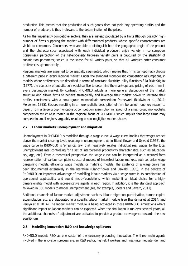
2.1 Product markets: segmentation and differentiation

Each region hosts industrial sectors with and without scope for product differentiation between varieties. Hence, the six different sectors of each regional economy are therefore split into two categories: perfectly competitive sectors producing homogeneous goods and imperfectly competitive sectors supplying differentiated varieties of the same goods. Firms in perfectly competitive, constant-returns-to-

scale sectors produce undifferentiated commodities and price at marginal costs. Firms in the imperfectly competitive, differentiated-goods sector produce specific varieties under increasing returns to scale. These firms can price discriminate their export markets and, given the small-group monopolistic competition structure, can set different levels of mark-ups in the different destination markets. The number of firms in each sector-region is empirically estimated through the national Herfindahl indices, assuming that all the firms within one region share the same technology. The main intuition is that firms with larger market shares are able to extract higher mark-ups from consumers than their competitors because of their higher weight in the price index. Hence, since market shares vary by destination market, mark-ups vary accordingly.

Perfectly competitive sectors are characterised by undifferentiated products supplied under constant

returns to scale. Consumers can distinguish the different origins of the product, so that the standard Armington assumption is respected, but they cannot distinguish individual providers of the good, which means that firms compete under perfect competition and charge a price equal to the marginal costs of

4 See Mercenier et al (2016) for a formal description of the latest version of the RHOMOLO model.

9

production. This means that the production of such goods does not yield any operating profits and the number of producers is thus irrelevant to the determination of the prices.

As for the imperfectly competitive sectors, they are instead populated by a finite (though possibly high) number of firms supplying the market with differentiated products, whose specific characteristics are visible to consumers. Consumers, who are able to distinguish both the geographic origin of the product and the characteristics associated with each individual producer, enjoy variety in consumption. Consumers' perception of the heterogeneity between variety pairs is captured by the elasticity of substitution parameter, which is the same for all variety-pairs, so that all varieties enter consumer preferences symmetrically.

Regional markets are assumed to be spatially segmented, which implies that firms can optimally choose a different price in every regional market. Under the standard monopolistic competition assumptions, in models where preferences are described in terms of constant elasticity utility functions à la Dixit-Stiglitz (1977), the elasticity of substitution would suffice to determine the mark-ups and pricing of each firm in every destination market. By contrast, RHOMOLO adopts a more general description of the market structure and allows firms to behave strategically and leverage their market power to increase their profits, consistently with a small-group monopolistic competition framework (Baldwin et al., 2011; Mercenier, 1995). Besides resulting in a more realistic description of firm behaviour, one key reason to depart from a large-group monopolistic competition assumption in favour of a small-group monopolistic competition structure is rooted in the regional focus of RHOMOLO, which implies that large firms may compete in small regions, arguably resulting in non-negligible market shares.

2.2 Labour markets: unemployment and migration

Unemployment in RHOMOLO is modelled through a wage curve. A wage curve implies that wages are set above the market clearing level, resulting in unemployment. As in Blanchflower and Oswald (1995), the wage curve in RHOMOLO is 'empirical law' that negatively relates individual real wages to the local unemployment rate (controlling for a set of interpersonal productivity characteristics, such as education, sex, age, etc.). From a theoretical perspective, the wage curve can be interpreted as a reduced-form representation of various complete structural models of imperfect labour markets, such as union wage bargaining models, efficiency wage models, or matching models. The existence of a wage curve has

been documented extensively in the literature (Blanchflower and Oswald, 1995). In the context of RHOMOLO, an important advantage of modelling labour markets via a wage curve is its combination of operational applicability and sound micro-foundations, which make it an ideal choice for a high-dimensionality model with representative agents in each region. In addition, it is the standard approach followed in CGE models to model unemployment (see, for example, Boeters and Savard, 2013).

Additional channels of labour market adjustment, such as labour migration, participation, human capital accumulation, etc. are elaborated in a specific labour market module (see Brandsma et al 2014; and Persyn et al 2014). The labour market module is being activated in those RHOMOLO simulations where significant impact on labour markets can be expected. When the simulation is run over several years, all the additional channels of adjustment are activated to provide a gradual convergence towards the new

equilibrium.

2.3 Modelling innovation: R&D and knowledge spillovers

RHOMOLO models R&D as one sector of the economy producing innovation. The three main agents involved in the innovation process are: an R&D sector, high-skill workers and final (intermediate) demand

10

of firms. The national R&D sector sells R&D services to firms in all the sectors of the economy located in the same country and uses a specific high-skill labour factor.

The production (and purchase) of R&D services generates positive spatial knowledge spillovers. In line with Leahy and Neary (2007), any innovative activity has an information component that is almost completely non-appropriable and costless to acquire, an idea dating back to Marshall (1920) and Nelson (1959). The introduction of this idea in general equilibrium models, though, is more recent, and has been introduces either splitting research activities into an appropriable and non-appropriable knowledge, as for example in Goulder and Schneider (1999) in the context of climate studies and Diao et al. (1999) based on a theory of endogenous growth, or based on the extension of product varieties such as Romer (1990), Grossman and Helpman (1991) and Aghion and Howitt (1992).

In RHOMOLO, there are spatial technology spillovers in the sense that the national R&D sector affects the total factor productivity of the regions within each country, which results in inter-regional knowledge spillovers from the stock of national accumulated knowledge. This positive externality derived from the accumulation of a knowledge stock in the country can benefit all regions to a different extent through sector-region specific spill-over elasticities.

2.4 New Economic Geography features

The structure of the RHOMOLO model engenders different endogenous agglomeration and dispersion patterns of firms by making the number of firms in each region endogenous (for details see Di Comite

and Kancs, 2014). Three effects drive the mechanics of endogenous agglomeration and dispersion of economic agents: the market access effect, the price index effect and the market crowding effect. The market access effect captures the fact that firms in central regions are closer to a large number of consumers (in the sense of lower iceberg transport costs) than firms in peripheral regions. The price index effect captures the impact of having the possibility of sourcing cheaper intermediate inputs because of the proximity of suppliers and the resulting price moderation because of competition. Finally, the market crowding effect captures the idea that, because of higher competition on input and output markets, firms can extract smaller mark-ups from their customers in central regions.

Whereas the first two forces drive the system of regional economies towards agglomeration by increasing the number of firms in core regions and decreasing it in the periphery, the third force causes

dispersion by reducing the margins of profitability in the core regions. However, in addition to these effects, which are common to theoretical New Economic Geography models with symmetric varieties, the specific characteristics of a spatial CGE model such as RHOMOLO implicitly add some stability in location patterns by calibrating consumer preferences over the different varieties in the base year. Through calibration, the regional patterns of intermediate and final consumption observed in a given moment of time are translated into variety-specific preference parameters, which ensure a given level of demand for varieties produced in each region, including peripheral ones. Therefore, it would be impossible to obtain extreme spatial configurations in terms of agglomeration or dispersion because firms in the regions with very low number of firms would enjoy very high operating profits due to the high level of consumer marginal provided by their relative scarce variety and thus would attract more firms in the

region.

2.5 Recursive dynamics and equilibria

Due to its high dimensionality, RHOMOLO is solved following a recursively dynamic approach. It contains a sequence of short-run equilibria that are related to each other through the build-up of physical and

11

human capital stocks. The extensive regional disaggregation of RHOMOLO implies that the dynamics have to be kept relatively simple. In contrast to QUEST, which is a fully dynamic model with inter-temporal optimisation of economic agents, the recursive approach followed in RHOMOLO implies that the optimisation problems in RHOMOLO are solved as inherently static and agents are backward- rather than forward-looking, which means that they can learn and adapt from the past experience (for example in the labour market) but do not make conjectures about the future. In each period the households make decisions about consumption, savings and labour supply in order to maximise their utility subject to budget constraint.

2.6 Performing policy simulations with RHOMOLO

There are two ways of performing policy simulations with the RHOMOLO model:

i. via a graphical web-interface; ii. via a GAMS-IDE interface.

The two options are associated with the same version of the RHOMOLO model. However, there are important differences in the simulation complexity and flexibility allowed by each option. When the model is solved using the General Algebraic Modelling System (GAMS) Integrated Development Environment (IDE) interface, all the technical details of the model can be adjusted and adapted to the simulation needs. By contrast, settings are fixed in the web-interface to allow users to obtain quick and easy results from a standard version of the model.

In other words, of the five steps presented in the introduction, using the graphical web-interface policy analysis jumps directly to step 3 (Calculation of counterfactual equilibrium) and step 4 (Policy appraisal based of comparison between the counterfactual and the base year equilibrium) because steps 1 and 2 are executed automatically by the system. This implies that also sensitivity analyses of key model parameter values (step 5) cannot be performed via the graphical web-interface, which allows only to obtain cumulative multipliers and spillover effects with baseline parameter values.

By contrast, using the GAMS-IDE interface all five steps of policy simulations can be followed with the RHOMOLO model.

3 POLICY SIMULATIONS VIA THE GRAPHICAL WEB-INTERFACE

In order to allow users to run simple simulations on a basic version of the model and have a first impression of the results that can be obtained with more problem-tailored versions of RHOMOLO, a graphical web-based interface has been developed and implemented for running the model. Registered users can visit the URL http://rhomolo.jrc.ec.europa.eu and simulate a simple set of policy shocks with RHOMOLO. The homepage of the web tool provides some information on the model in the "About" page (accessible through the corresponding tab). Figure 2 provides a screenshot of the RHOMOLO homepage:

12

Figure 2: Homepage of the RHOMOLO web-interface

Clicking on "sign in", users are redirected to the authentication page, where the European Commission

Authentication Service (ECAS) username and password have to be introduced.

Figure 3: ECAS authentication for web-interface

13

3.1 Step 3 - Calculation of counterfactual equilibrium

The graphical web interface offers registered users the following three options for introducing policy shocks (see Figure 4):

- "Run the model with global values for policy shocks", which amounts to introducing a common policy shock to all regions;

- "Upload a file with regional values" to introduce region-specific policy shocks; - "Use a job identifier" to retrieve a previously executed and saved policy simulation.

With the first option, the user can introduce a common policy shock to all the EU NUTS2 regions. There are two ways how the policy shock can be introduced. First, the user can directly allocate a specific

amount of EU policy expenditures (in million €) to each region and policy type. Currently, the number of policy types which can be simulated using the graphical web-interface has been limited to three (human capital, transport infrastructure and R&D and innovation policies). For simulations involving other types of EU policies the more advanced GAMS-IDE interface need to be used, which offers many more possibilities / aggregation schemes of introducing policy instruments into RHOMOLO. Second, if the user knows which model variables are affected by how much from each type of policy, the policy shock can be introduced through the respective model variables. As above, the number of policy types which can be simulated using the graphical web-interface has been limited to three: increase in total factor productivity, increase in labour productivity and reduction of transportation costs, which correspond to investments in R&D and innovation, human capital and transport infrastructure, respectively. For

practical reasons, on the web interface the magnitude of the "Total Factor Productivity", "Labour Productivity" or "Transport Costs" shocks has currently been restricted between -5% and +5%, to ensure that the model will converge fast and deliver easily interpretable results;

The second option allows the user to introduce region-specific policy shocks, by downloading the template in CSV format and introducing manually the shock (between -5% and +5%) to the three types of policies (human capital, R&D and innovation and transport infrastructure) of any EU NUTS2 region. After the template is downloaded and filled with the shocks to be simulated, it should be uploaded in the system by clicking on the corresponding command icon, which will run the model simulation with the

desired shocks;5

Finally, the third option consists in recalling a RHOMOLO simulation that has been run and saved in the past, when the user is only interested in the output of a previous simulation without having to wait for the model to solve again. In this case, the user can simply introduce the identifier number in the "identifier" tab and will be redirected to the output of previous simulations.

5 Please notice that, depending on the version of Microsoft Excel used, opening the template file ("user-input.csv") may result in some region names to be read as different items (i.e. dates) and thus result in errors when the file is uploaded. One easy way to avoid this little annoyance is to open the .csv file in notepad.

14

Figure 4: Selection of policy shocks

3.2 Step 4 - Policy appraisal based on comparison between the counterfactual and the

baseline projections

After running the simulation, the output is provided in two formats: as a map and as an Excel table. In both cases, the results are expressed as the difference between the base line equilibrium and the counterfactual equilibrium. When the results as displayed as a map, EU regions are displayed with

different shades of colour for the different regions depending on the underlying values of the variable selected (see Figures 5 and 6). The identifier of the simulation is provided on top of the simulation page, (which is the code that has to be introduced in the "use job identifier pane" to later retrieve the output of the simulation). Then, between the identifier and the map, the options to run a new simulation or introduce another identifier are displayed. Finally, on the bottom of the page the map with results and additional information on the simulation are available.

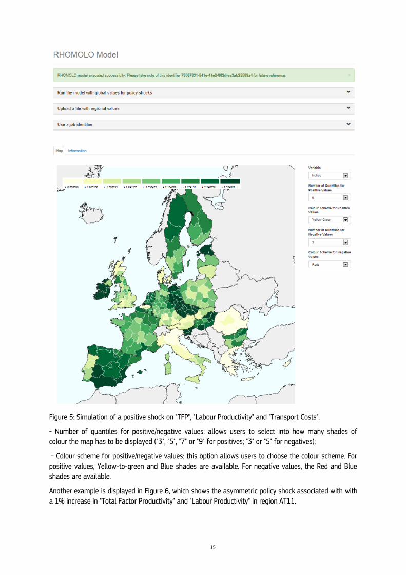
As an example of a map with RHOMOLO results, where 1% positive shock on "Total Factor Productivity", "Labour Productivity" and "Transport Costs" is simulated, is displayed in Figure 5. On the right-hand side of the screen there are several visualisation options of simulation results:

- Variable: to select which output has to be displayed on the map (as percentage deviations from the

baseline). Household income ("inchou"), wages of the high-skill ("wage_H"), medium-skill ("wage_M") and low-skill ("wage_L") workers can be selected;

15

Figure 5: Simulation of a positive shock on "TFP", "Labour Productivity" and "Transport Costs".

- Number of quantiles for positive/negative values: allows users to select into how many shades of colour the map has to be displayed ("3", "5", "7" or "9" for positives; "3" or "5" for negatives);

- Colour scheme for positive/negative values: this option allows users to choose the colour scheme. For positive values, Yellow-to-green and Blue shades are available. For negative values, the Red and Blue

shades are available.

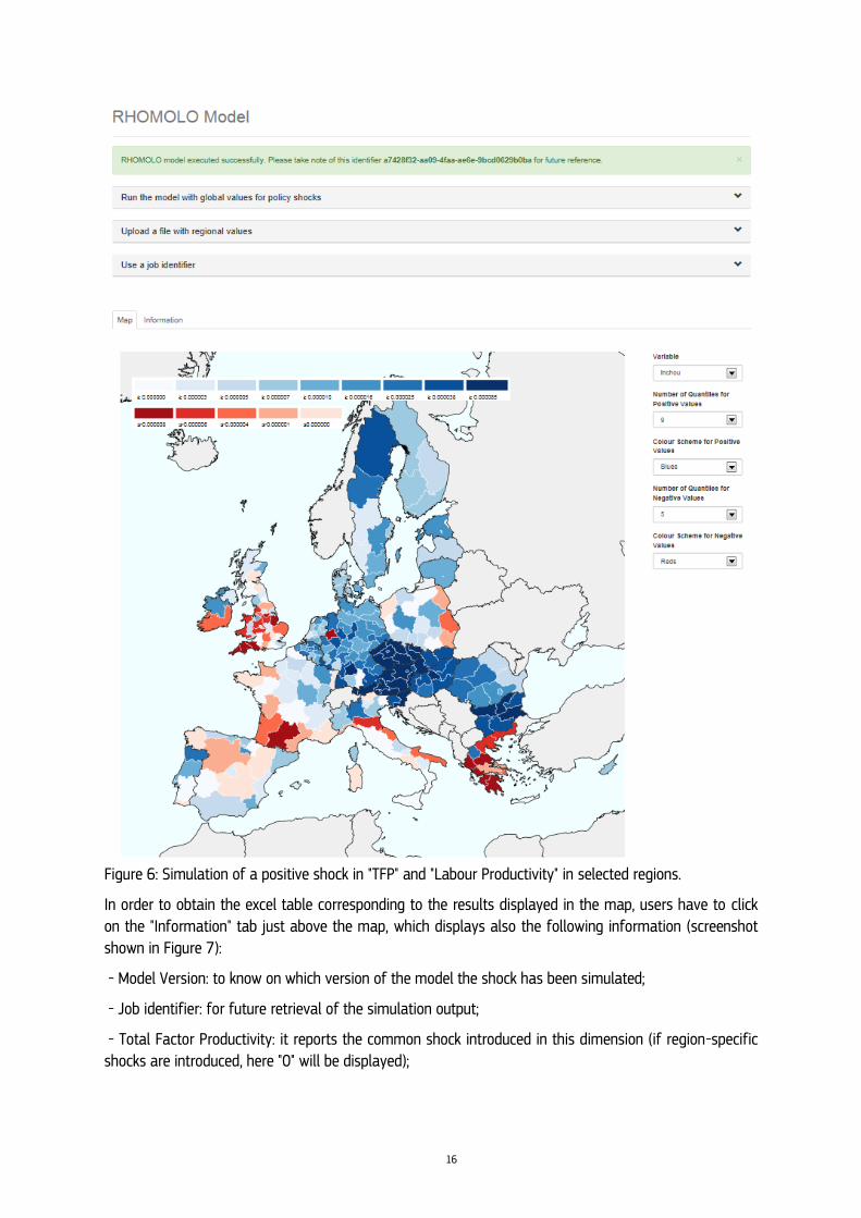
Another example is displayed in Figure 6, which shows the asymmetric policy shock associated with with a 1% increase in "Total Factor Productivity" and "Labour Productivity" in region AT11.

16

Figure 6: Simulation of a positive shock in "TFP" and "Labour Productivity" in selected regions.

In order to obtain the excel table corresponding to the results displayed in the map, users have to click on the "Information" tab just above the map, which displays also the following information (screenshot shown in Figure 7):

- Model Version: to know on which version of the model the shock has been simulated;

- Job identifier: for future retrieval of the simulation output;

- Total Factor Productivity: it reports the common shock introduced in this dimension (if region-specific shocks are introduced, here "0" will be displayed);

17

- Labour Productivity: it reports the common shock introduced in this dimension (if region-specific shocks are introduced, here "0" will be displayed);

- Transport Costs: it reports the common shock introduced in this dimension (if region-specific shocks are introduced, here "0" will be displayed);

- Status: it shows whether the simulation has been run successfully (by reporting "Success");

- Start date: it indicates the moment in which the simulation has been started;

- End date: it indicates the moment in which the simulation has been completed;

- Extended log: it allows users to see the output of GAMS associated with the simulation.

The excel table can be obtained by clicking on "Output data file", which sends a .csv file with the regional deviations from the baseline in household income ("inchou"), wages of the high-skill ("wage_H"), medium-skill ("wage_M") and low-skill ("wage_L") workers.

Figure 7: Screenshot of "Information" tab.

18

4 POLICY SIMULATIONS VIA THE GAMS-IDE INTERFACE

We turn now to the description of how to use the General Algebraic Modelling System (GAMS) Integrated Development Environment (IDE) interface for performing policy simulations with RHOMOLO. First, we provide a brief overview of how the RHOMOLO model is implemented in the GAMS-IDE environment. Second, the structure of RHOMOLO files and folders is explained. Finally, a step-by-step explanation is provided on how to run the RHOMOLO model via the GAMS-IDE interface.

4.1 RHOMOLO setup in GAMS-IDE

The GAMS-IDE is an interface designed to create, debug, edit and run GAMS files. It permits to launch

and monitor the compilation and execution of models that are written in GAMS. GAMS-IDE provides a convenient and simple access to the model code. The progress of a compilation/execution process can be monitored directly in the GAMS process window (which can be used also for navigation in the GAMS source code, listing or log files). When policy simulations with a .gms source code are completed, GAMS produces model files that have the name of a source GAMS file and extensions .lst, .log and .lxi:

.lst files contain model outputs such as a list of equations, the reported values of parameters, scalars, variables and etc.;

.log files provide information about the solution and possible error status;

.lxi files contain navigation information that is used by GAMS-IDE to generate the navigation window that permits to browse the entries of the .lst file.

With GAMS-IDE it is possible to efficiently locate potential errors in the GAMS code. Double-clicking on the lines in the GAMS process window allows users to access the output. For example, clicking on the blue lines opens the associated listing .lst file, clicking on the red lines redirects to the line in a .gms source file where the error occurred.

In what follows, we briefly describe how to customise the GAMS-IDE interface for running RHOMOLO, relating it to the five CGE modelling steps described in the introduction.

After opening the GAMS-IDE application for the first time, a number of preliminary actions should be taken to make the most of executing RHOMOLO in GAMS. Press the button File in the top left corner of GAMS-IDE and click on Options in the fall down menu.

In the "Options" menu, users can customize syntax. For example, it can be decided to have data, comments, reserved words, strings and explanatory text displayed in different colours. Similarly, the type and size of fonts is customisable, as is the page format and the path to the location of GAMS license..

One important step to customise the GAMS-IDE interface for running RHOMOLO consists in opening the tab "File \Options \Solvers" and clicking on the cell [CONOPT; NLP], scrolling down, clicking on the cell [PATH; MCP] and then confirming with the OK button. This step associates solvers CONOPT and MCP with a given class of mathematical problems such as nonlinear programming (NLP) or mixed complementarity programming (MCP). A screenshot is shown in Figure 8.

19

Figure 8: Selection of default RHOMOLO solvers in GAMS-IDE

We recommend that in the tab "File \Options \Execute" a user selects the option "Minimised" in the drop down menu of DOS window (marked with a red arrow). This option makes a DOS window visible in the

programme bar (as indicated with a blue arrow in Figure 9). The DOS window bar remains active while the model runs and disappears when policy simulations are terminated. One convenience of having a DOS window activated is that the user does not need to watch the IDE process window to see when the model execution is finished. Instead, the user can work on other tasks or applications, giving a fast glance at the DOS window bar at the bottom of computer screen, as pointed with blue arrow above.

Figure 9: Activation of DOS window in GAMS-IDE

20

4.2 RHOMOLO file organisation

Large, complex, multi-dimensional models, such as RHOMOLO, are usually associated with long computer codes that may be difficult to navigate, edit and manage. In RHOMOLO all adjustments of input data and the reporting of model output are entirely coded in GAMS. Therefore, in order to improve the readability and organisation of the RHOMOLO GAMS code, we have adopted a modular approach. The basic idea behind the modular approach is to split the model code into several stand-alone modules that perform different tasks in RHOMOLO, as for example:

- Read in the SAMs of the EU Members States into the GAMS model code; - Read in the matrices of trade costs and inter-regional trade flows;

- Re-balance the inter-regional trade flows to match the country data on domestic sales and trade within the EU;

- Construct regional SAMs using regional and national data, parameterise the model; - Run the core model to reproduce the base-year equilibrium; - Run counterfactual model scenarios (in static or in dynamic settings); - Report changes in macroeconomic indicators and cumulative policy multipliers; - Send the results to Excel.

The adopted modular structure of RHOMOLO significantly improves the efficiency of developing and using the model. First of all, it increases the tractability of the model code, as the code is divided into thematic modules. Different modules can be simultaneously opened in the GAMS-IDE or any editor which

simplifies their reading or editing. Second, it is much faster to design, implement and test the modules individually, instead of running the whole model. Third, the modular structure makes it simple to merge changes when several modellers are working on different parts of the model.

The version-control and merge processes are achieved using the Apache Subversion (SVN) client TortoiseSVN software, which permits to trace changes in a source code that were implemented by different users and to maintain current and historical versions of files.

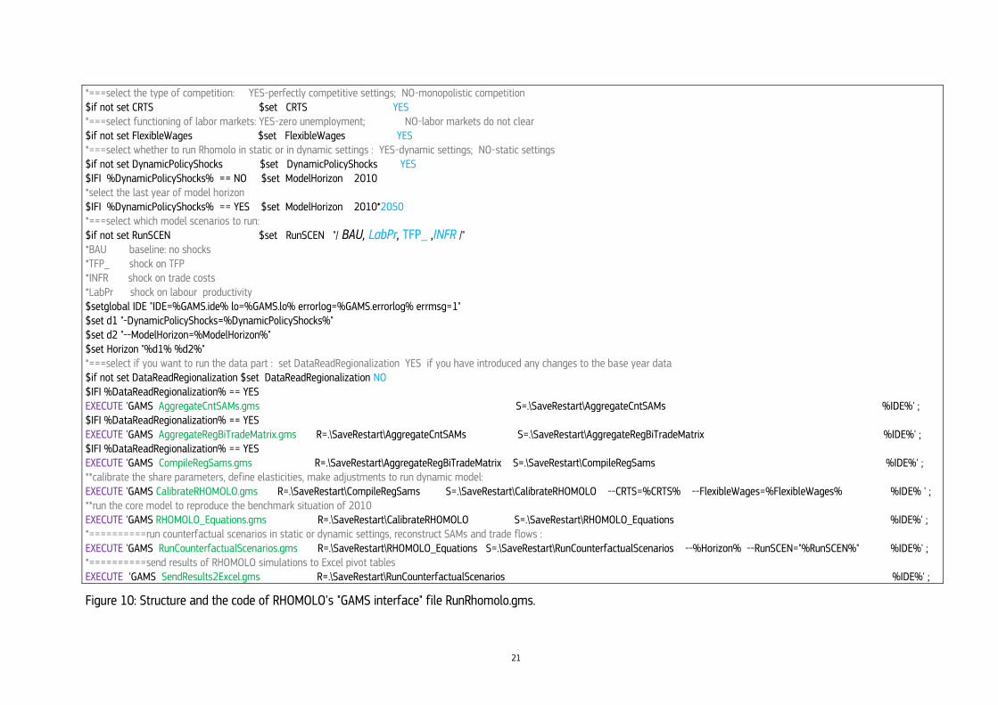
The main file a user needs to run for performing policy simulations with RHOMOLO in GAMS-IDE is RunRHOMOLO.gms. The file RunRHOMOLO.gms acts like a GAMS "user interface" that manages execution of modules in a specified order and permits also unexperienced users to modify the model

settings. There are different features of the model that can be altered by changing the settings, as for example the type of product competition, the functioning of labour markets, the time horizon and the definition of counterfactual scenarios are. In accordance with the chosen model settings, the "user interface" file RunRHOMOLO.gms runs the modules which are connected with the sequence of EXECUTE commands and user-defined save and restart options. Below we briefly explain the structure of file RunRHOMOLO.gms and show how to customise the RHOMOLO model settings. Those items that the user has to select in order to define model settings for the current policy simulations with RHOMOLO are highlighted in blue, as shown in Figure 10.

21

*===select the type of competition: YES-perfectly competitive settings; NO-monopolistic competition $if not set CRTS $set CRTS YES *===select functioning of labor markets: YES-zero unemployment; NO-labor markets do not clear $if not set FlexibleWages $set FlexibleWages YES *===select whether to run Rhomolo in static or in dynamic settings : YES-dynamic settings; NO-static settings $if not set DynamicPolicyShocks $set DynamicPolicyShocks YES $IFI %DynamicPolicyShocks% == NO $set ModelHorizon 2010 *select the last year of model horizon $IFI %DynamicPolicyShocks% == YES $set ModelHorizon 2010*2050 *===select which model scenarios to run: $if not set RunSCEN $set RunSCEN "/ BAU, LabPr, TFP_ ,INFR /" *BAU baseline: no shocks *TFP_ shock on TFP *INFR shock on trade costs *LabPr shock on labour productivity $setglobal IDE "IDE=%GAMS.ide% lo=%GAMS.lo% errorlog=%GAMS.errorlog% errmsg=1" $set d1 "-DynamicPolicyShocks=%DynamicPolicyShocks%" $set d2 "--ModelHorizon=%ModelHorizon%" $set Horizon "%d1% %d2%" *===select if you want to run the data part : set DataReadRegionalization YES if you have introduced any changes to the base year data $if not set DataReadRegionalization $set DataReadRegionalization NO $IFI %DataReadRegionalization% == YES EXECUTE 'GAMS AggregateCntSAMs.gms S=.\SaveRestart\AggregateCntSAMs %IDE%' ; $IFI %DataReadRegionalization% == YES EXECUTE 'GAMS AggregateRegBiTradeMatrix.gms R=.\SaveRestart\AggregateCntSAMs S=.\SaveRestart\AggregateRegBiTradeMatrix %IDE%' ; $IFI %DataReadRegionalization% == YES EXECUTE 'GAMS CompileRegSams.gms R=.\SaveRestart\AggregateRegBiTradeMatrix S=.\SaveRestart\CompileRegSams %IDE%' ; **calibrate the share parameters, define elasticities, make adjustments to run dynamic model: EXECUTE 'GAMS CalibrateRHOMOLO.gms R=.\SaveRestart\CompileRegSams S=.\SaveRestart\CalibrateRHOMOLO --CRTS=%CRTS% --FlexibleWages=%FlexibleWages% %IDE% ' ; **run the core model to reproduce the benchmark situation of 2010 EXECUTE 'GAMS RHOMOLO_Equations.gms R=.\SaveRestart\CalibrateRHOMOLO S=.\SaveRestart\RHOMOLO_Equations %IDE%' ; *==========run counterfactual scenarios in static or dynamic settings, reconstruct SAMs and trade flows : EXECUTE 'GAMS RunCounterfactualScenarios.gms R=.\SaveRestart\RHOMOLO_Equations S=.\SaveRestart\RunCounterfactualScenarios --%Horizon% --RunSCEN="%RunSCEN%" %IDE%' ; *==========send results of RHOMOLO simulations to Excel pivot tables EXECUTE 'GAMS SendResults2Excel.gms R=.\SaveRestart\RunCounterfactualScenarios %IDE%' ;

Figure 10: Structure and the code of RHOMOLO's "GAMS interface" file RunRhomolo.gms.

22

Control variables are initialised with $set or $setglobal commands, which are statements used to

activate or deactivate certain model features. The RHOMOLO model is executed in accordance with the values that are assigned to the control variables in file RunRHOMOLO.gms. Below are summarised the

values of those RHOMOLO settings users have to select to adjust the model settings for the simulation:6

$set CRTS YES/NO

$set FlexibleWages YES/NO

$set DynamicPolicyShocks YES/NO

$set RunSCEN "/ BAU, LabPr, TFP_ , INFR /"

$set ModelHorizon 2010*2050

$set DataReadRegionalization YES/NO

With the command statement "$set CRTS YES" RHOMOLO solves with a perfectly competitive product market (Constant Returns To Scale (CRTS)), whereas "$set CRTS NO" allows imperfect competition in selected sectors (as specified in file CalibrateRHOMOLO.gms, in the current version those sectors are manufacturing and construction, business services, transport and trade).

The command statement "$set FlexibleWages YES" activates flexible wages and zero unemployment; "$set FlexibleWages NO" activates unemployment in RHOMOLO, which as explained in section 2 is modelled via a wage curve. When the simulation spans over several years, wages do not adjust instantaneously to changes in unemployment but include a gradual mechanism of adjustment towards the new steady state.

The command statement "$set DynamicPolicyShocks NO" limits the time horizon of the simulation to one year (2010), as determined in the following command line: "$IFI %DynamicPolicyShocks% == NO

$set ModelHorizon 2010". By contrast, the command statement "$set DynamicPolicyShocks YES" allows the model to run the simulation runs over more years. In this case, the exact time horizon can be chose by the user in the command line "$IFI %DynamicPolicyShocks% == YES $set ModelHorizon 2010*2050", by changing the last term, 2050 in our example.

The specific model scenarios to simulate can be selected in the command line "$if not set RunSCEN $set RunSCEN /BAU, LabPr, TFP_ ,INFR / ". The selected scenarios can be any subset of /BAU, INFR, TFP_, LabPr/, where BAU stands for Business As Usual (the baseline); LabPr indicates human capital policies; TFP_ is usd for R&D and innovation policies; INFR for infrastructure policies. The user can run simulations with one or more policy shocks. In our example, changes in all the policy types are included. In order to evaluate changes in macroeconomic indicators for the counterfactual scenarios with respect to the baseline values, the baseline scenario BAU should always be in the list of model scenarios to simulate.

The command statement "$setglobal IDE "IDE=%GAMS.ide% lo=%GAMS.lo% errorlog=%GAMS.errorlog% errmsg=1" prompts the creation of .lst, .log and .lxi files for all GAMS modules that are run with execute commands. This command statement permits users to navigate through the output of executed files in GAMS-IDE.

6 These settings are the ones most frequently used in RHOMOLO. Generally, there are many more RHOMOLO settings that can be adjusted through the GAMS code.

23

In order to run the RHOMOLO model from GAMS-IDE,7 the project file Rhomolo.gpr needs to be opened.

The extension .gpr indicates that Rhomolo.gpr is a project file. The location of the project file determines the directory where all saved files are placed and where GAMS looks for files when running the model. It also stores the information about which files were opened when the project was last closed, in order to restore these windows in the same state when the project is launched again.

Once the model project file is active, the user has to open RunRHOMOLO.gms, select model settings (as it explained above), and to press F9 or to click on the run button on the top menu of GAMS-IDE. Having a DOS window activated, the user can watch the progress while policy simulations with RHOMOLO are carried out. Figure 11 displays a screenshot of the DOS window that shows model progress in running for a given year and a given model scenario.

Figure 11: Screenshot of DOS window

All files needed to run the RHOMOLO model are stored in the folder \ RHOMOLO (see Figure 12):

Figure 12: Content of the main RHOMOLO model folder

Below we provide a short description of each model file. All RHOMOLO data are stored in a sub-folder RHOMOLO\Data (see Figure 13):

7 Alternatively, the user can run model from a MS-DOS batch file, which neither requires launching the GAMS-IDE, nor opening the project file. Examples of batch scripts to run RHOMOLO are provided in the section 4.3.

24

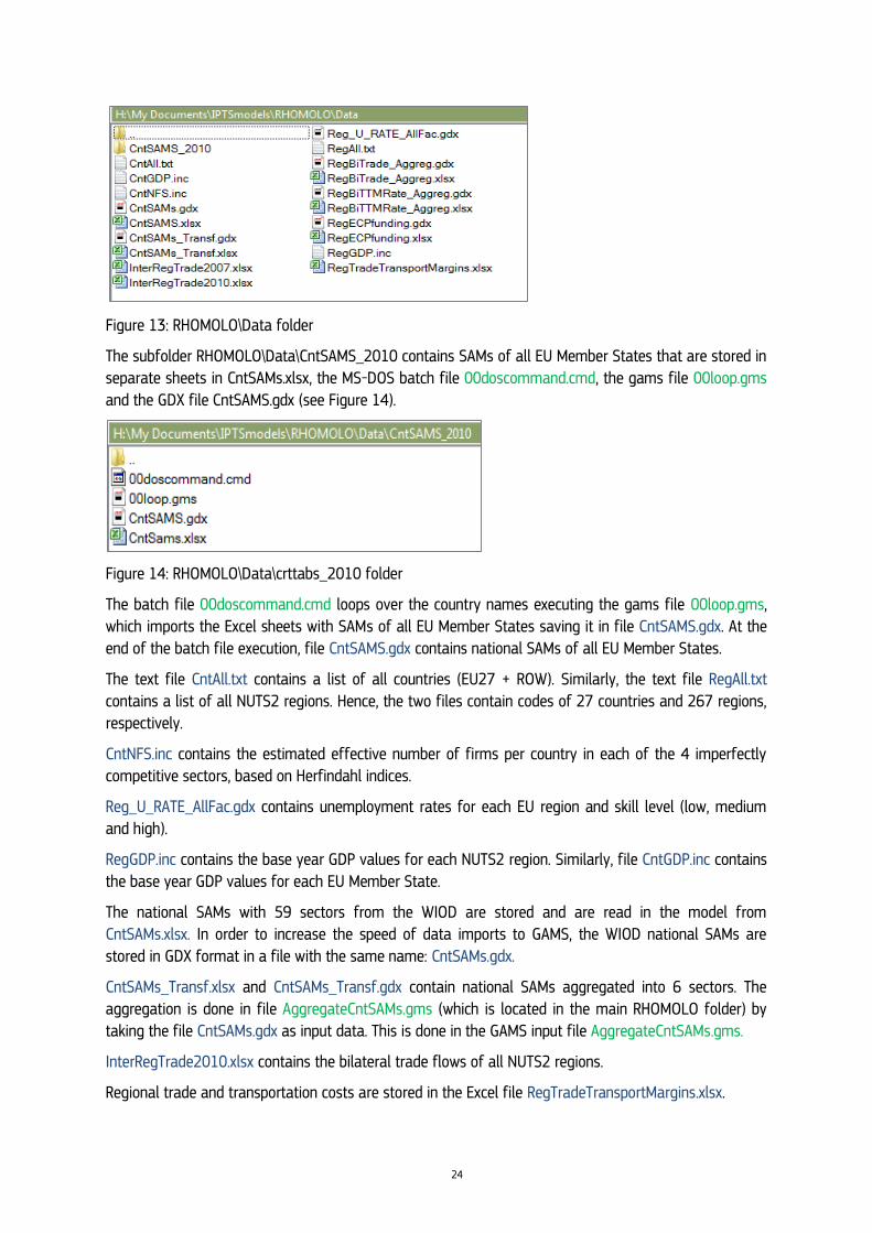
Figure 13: RHOMOLO\Data folder

The subfolder RHOMOLO\Data\CntSAMS_2010 contains SAMs of all EU Member States that are stored in separate sheets in CntSAMs.xlsx, the MS-DOS batch file 00doscommand.cmd, the gams file 00loop.gms

and the GDX file CntSAMS.gdx (see Figure 14).

Figure 14: RHOMOLO\Data\crttabs_2010 folder

The batch file 00doscommand.cmd loops over the country names executing the gams file 00loop.gms, which imports the Excel sheets with SAMs of all EU Member States saving it in file CntSAMS.gdx. At the end of the batch file execution, file CntSAMS.gdx contains national SAMs of all EU Member States.

The text file CntAll.txt contains a list of all countries (EU27 + ROW). Similarly, the text file RegAll.txt contains a list of all NUTS2 regions. Hence, the two files contain codes of 27 countries and 267 regions, respectively.

CntNFS.inc contains the estimated effective number of firms per country in each of the 4 imperfectly competitive sectors, based on Herfindahl indices.

Reg_U_RATE_AllFac.gdx contains unemployment rates for each EU region and skill level (low, medium and high).

RegGDP.inc contains the base year GDP values for each NUTS2 region. Similarly, file CntGDP.inc contains the base year GDP values for each EU Member State.

The national SAMs with 59 sectors from the WIOD are stored and are read in the model from CntSAMs.xlsx. In order to increase the speed of data imports to GAMS, the WIOD national SAMs are

stored in GDX format in a file with the same name: CntSAMs.gdx.

CntSAMs_Transf.xlsx and CntSAMs_Transf.gdx contain national SAMs aggregated into 6 sectors. The aggregation is done in file AggregateCntSAMs.gms (which is located in the main RHOMOLO folder) by taking the file CntSAMs.gdx as input data. This is done in the GAMS input file AggregateCntSAMs.gms.

InterRegTrade2010.xlsx contains the bilateral trade flows of all NUTS2 regions.

Regional trade and transportation costs are stored in the Excel file RegTradeTransportMargins.xlsx.

25

Input data are read-in and processed in AggregateCntSAMs.gms, AggregateRegBiTradeMatrix.gms and

CompileRegSams.gms.

The GAMS input file AggregateRegBiTradeMatrix.gms imports the bilateral regional trade flows data from InterRegTrade_2010.xlsx and the regional bilateral trade cost rates RegTradeTransportMargins.xlsx, re-aggregates the sectors (if needed for computational or robustness reasons) and saves the output into RegBiTrade_Aggreg.gdx and RegBiTTMRate_Aggreg.gdx. Hence, RegBiTrade_Aggreg.xlsx and RegBiTrade_Aggreg.gdx are the result of aggregation of bilateral trade flows (inclusive of trade and transport margins) for all NUTS2 regions and tradable sectors. Analogously, RegBiTTMRate_Aggreg.xlsx and RegBiTTMRate_Aggreg.gdx are the result of aggregation of bilateral trade flows and transportation costs (rates) for all NUTS2 regions and tradable sectors.

The GAMS input file CompileRegSams.gms constructs regional SAMs by using the regional and national data stored in files CntSAMs_Transf.gdx, RegBiTrade_Aggreg.gdx, RegBiTTMRate_Aggreg.gdx, RegData.inc and RegGDP.inc.

When working with large, complex and computationally intense models such as RHOMOLO, a good programming practice is to divide the code into several parts and execute them using the "save and restart" options. These options allow users to run parts of the model, save the solution point and move to the next part of the code (at any time in the future) from the last saved solution point. In the RHOMOLO folder, all the files with extension .g00 are "work files" that preserve all the information about the saved solution point (including declarations, values, option settings and compiler directives) known to GAMS at the end of their corresponding run. The basic function of a work file is to preserve information that has been resource-intensive to produce (in terms of memory allocation and time). When restarting from the work file, GAMS reads the work file .g00 and restores the information kept in the associated

.gms file.8 All .g00 files that contain saved solution points are stored in RHOMOLO\SaveRestart folder

(shown in Figure 15).

Figure 15: RHOMOLO\ SaveRestart folder

When opened, .g00 files do not provide any interpretable information for the user. They are encoded intermediate, mostly binary, files that are used internally by the GAMS software.

Save and restart options can be set up either in the command line of GAMS IDE or directly in the .gms file using the $call or execute commands. Using the first option, save and restart parameters have to be

defined in the command line of each file. However, when a working GAMS file is renamed or a project file is deleted, save and restart options automatically disappear from the command line and have to be set up anew. The redefinition of save and restart options is inconvenient when different draft versions of files with different names are created, or used by different modellers. Therefore, in RHOMOLO we prefer

8 Work files should be re-run anew when moving from one version of GAMS to another.

26

to combine all save and restart commands in a single GAMS file RunRHOMOLO.gms with $call or execute

commands. In this case, the save and restart commands do not disappear.

The choices about the type of competition and functioning of labour markets selected in the "user interface file" RunRHOMOLO.gms are passed on to the file CalibrateRHOMOLO.gms. The choices concerning model scenarios and model horizon are passed on to RunCounterfactualScenarios.gms.

The module CalibrateRHOMOLO.gms contains, amongs others:

- the code for the estimation of share parameters that enter RHOMOLO equations; - the list of model variables; - the values of elasticities; - the necessary adjustments to run the model in recursive-dynamic settings; - the selection of sectors that can function in monopolistically competitive settings, when this option

is activated in RunRHOMOLO.gms.

The equations determining the equilibrium conditions for the regional economies are contained in RHOMOLO_Equations.gms.

The counterfactual equilibria for the policy scenarios selected in the "user interface file" RunRHOMOLO.gms are computed in RunCounterfactualScenarios.gms. This module includes files InitializePa4Reporting.gms, ReconstructRegSAMs.gms and ReportMacroIndicators.gms,.

InitializePa4Reporting.gms lists variables and macroeconomic indicators, which are reported in terms of percentage changes with respect to the baseline.

ReportMacroIndicators.gms computes and reports macro indicators (e.g. region's GDP, household consumption and disposable income, production, exports, imports, terms of trade and cumulative policy multipliers) for the baseline and counterfactual scenarios.

The code for reconstructing the regional SAMs (after solving the model) for each region, year and policy scenario is contained in file ReconstructRegSAMs.gms.

SendResults2Excel.gms contains the GAMS code that stores the results of policy simulations in GDX format and exports them to Excel pivot tables. The exported results of policy simulations are stored as Excel and GDX files in folder RHOMOLO\RESULTS (see Figure 16).

Figure 16: RHOMOLO\RESULTS folder

The .gdx files are retrieved from GAMS in a same way as the .gms files. The parameter and variable values can be directly saved from the opened .gdx file as filtered or non-filtered Excel files (see Figure 17).

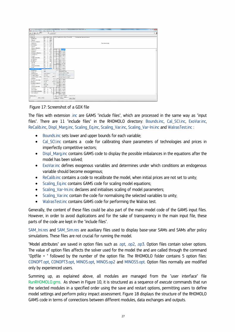
27

Figure 17: Screenshot of a GDX file

The files with extension .inc are GAMS "include files", which are processed in the same way as "input files". There are 11 "include files" in the RHOMOLO directory: Bounds.inc, Cal_SCI.inc, ExoVar.inc, ReCalib.inc, Displ_Marg.inc, Scaling_Eq.inc, Scaling_Var.inc, Scaling_Var-Ini.inc and WalrasTest.inc :

Bounds.inc sets lower and upper bounds for each variable;

Cal_SCI.inc contains a code for calibrating share parameters of technologies and prices in imperfectly competitive sectors;

Displ_Marg.inc contains GAMS code to display the possible imbalances in the equations after the model has been solved;

ExoVar.inc defines exogenous variables and determines under which conditions an endogenous

variable should become exogenous;

ReCalib.inc contains a code to recalibrate the model, when initial prices are not set to unity;

Scaling_Eq.inc contains GAMS code for scaling model equations;

Scaling_Var-Ini.inc declares and initialises scaling of model parameters;

Scaling_Var.inc contain the code for normalising the selected variables to unity;

WalrasTest.inc contains GAMS code for performing the Walras test.

Generally, the content of these files could be also part of the main model code of the GAMS input files. However, in order to avoid duplications and for the sake of transparency in the main input file, these parts of the code are kept in the "include files".

SAM_Ini.res and SAM_Sim.res are auxiliary files used to display base-year SAMs and SAMs after policy simulations. These files are not crucial for running the model.

"Model attributes" are saved in option files such as .opt, .op2, .op3. Option files contain solver options. The value of option files affects the solver used for the model the and are called through the command

"Optfile = " followed by the number of the option file. The RHOMOLO folder contains 5 option files: CONOPT.opt, CONOPT3.opt, MINOS.opt, MINOS.op2 and MINOS5.opt. Option files normally are modified only by experienced users.

Summing up, as explained above, all modules are managed from the "user interface" file RunRHOMOLO.gms. As shown in Figure 10, it is structured as a sequence of execute commands that run the selected modules in a specified order using the save and restart options, permitting users to define model settings and perform policy impact assessment. Figure 18 displays the structure of the RHOMOLO GAMS code in terms of connections between different modules, data exchanges and outputs.

28

Figure 18: RHOMOLO file organisation.

CntSAMs_Transf.xlsx, CntSAMs_Transf.gdx

CompileRegSAMs.g00

CalibrateRHOMOLO.gms

AggregateRegBiTradeMatrix.gms

CntAll.txt, CntSAMs.gdx

RegAll.txt, InterRegTrade2010.xlsx, RegTradeTransportMargins.xlsx

RegGDP.inc, CntNFS.inc, CntGDP.inc, Reg_U_RATE_AllFac.gdx, CntSAMs_Transf.gdx

AggregateCntSAMs.gms

RegBiTrade_Aggreg.xlsx; RegBiTrade_Aggreg.gdx, RegBiTTMRate_Aggreg.xlsx; RegBiTTMRate_Aggreg.gdx

CompileRegSAMs.gms

CalibrateRHOMOLO.g00

RHOMOLO_Equations.gms RHOMOLO_Equations.g00

RunCounterfactualScenarios .g00

AggregateCntSAMs.g00

AggregateRegBiTradeMatrix.g00

RunCounterfactualScenarios.gms

SendResults2Excel.gms

RegECPfunding.xlsx, InitializationPa4Reporting.gms, ReportMacroIndicators.gms,

ReconstructSAMs.gms

ResultsScn.xlsx

Scaling_Eq.inc, Bounds.inc, ExoVar.inc

Scaling_Var-Ini.inc, CAL_SCI.inc, Scaling_Var.inc, WalrasTest.inc, ReCalib.inc, Bounds.inc, ExoVar.inc

ReconstructedSAMs.csv, ReconstBilatTrade.xlsx, ReconstBilatTrade.gdx

29

4.3 Running policy simulations with RHOMOLO in GAMS-IDE

In this section, we report the steps to follow to perform policy simulations with RHOMOLO in GAMS-IDE.

4.3.1 Step 1 - Compilation of micro-consistent base year data

As a first step, a micro-consistent dataset is compiled, describing all the regional economies in the base year. As usual in CGE models, the base-year database of RHOMOLO is organised in form of regional Social Accounting Matrices (see Thissen et al, 2014), which are complemented with other data, such as bilateral trade flows, bilateral transportation costs, unemployment rates, number of firms.

Reading in and reconstructing the base-year data base is done in file RunRHOMOLO.gms. When the "$set

DataReadRegionalization" is set to "YES" in the "user interface" file RunRHOMOLO.gms, the model executes files AggregateCntSAMs.gms, AggregateRegBiTradeMatrix.gms, and CompileRegSams.gms. These modules contain the GAMS commands to read the Social Accounting Matrices (SAMs) of all EU Member States into the model code, the matrices of interregional trade flows and the transportation costs. It then reads in the regional data and compiles the regional SAMs for all NUTS2 regions, rebalancing the regional trade flows so that they are consistent with regional exports and imports.

Unless the input data are changed, there is no need to re-run these modules every time when policy simulations with RHOMOLO are carried out. Instead, these files can be executed only once. In order to skip the execution of modules AggregateCntSAMs.gms, AggregateRegBiTradeMatrix.gms and CompileRegSams.gms, the command statement in file RunRHOMOLO.gms needs to be set to "$set

DataReadRegionalization NO". The model will restart simulations from the previously saved solution point that is stored in RHOMOLO subfolder \SaveRestart.

Notice, however, that if the user is not working on a same version of GAMS on which the work files AggregateCntSAMs.g00, AggregateRegBiTradeMatrix.g00 and CompileRegSams.g00 were created, the user has to re-run them by setting "$set DataReadRegionalization YES ".

4.3.2 Step 2 – Calibration of the model

As a second step, all free parameters of the model are determined through a calibration procedure that yields a set of parameter values replicating the base-year equilibrium of all the model variables observed in the SAMs using the model equations.

The calibration of RHOMOLO is done using the regional SAMs for 2010 as a benchmark.9 The data

provided in the columns of the SAMs are used to calibrate the optimisation functions describing the behaviour of economic agents in accordance with the selected functional forms. The data in the rows describe market-clearance conditions to set the equality between supply and demand of each good. In addition, information on parameter values, such as elasticities, is needed to calibrate the model. These parameters are estimated econometrically or, where not possible due to data limitations, borrowed from the literature.

As usual in CGE models, all prices are indexed to unity in the base year, and all values in the SAMs are treated as benchmark quantities. These assumptions allow solving the model directly for technical

coefficients and preference parameters of the production (cost) and utility functions, respectively

9 Currently, the base year of the RHOMOLO model is being updated to 2013. This updated will increase both the number of NUTS2 regions and the number of NACE2 industrial sectors.

30

(Mansur and Whalley, 1983). In the tradition of CGE models, only the relative price changes are defined in RHOMOLO.

A cost minimisation problem subject to the chosen production technology (CES, Cobb-Douglas, Leontief, etc.) is solved to obtain normalised unit cost functions with given cost shares. The share parameters can be calibrated using model equations and the base-year values of all variables, or computed directly from the SAMs. For the normalisation of cost functions and calibration of cost shares the approach of Sancho (2009) has been adopted. Note that in RHOMOLO, in order to describe the behaviour of economic agents, we prefer to employ the normalised unit cost functions rather than production or consumption functions. As noted by Chambers (1988), the dual approach simplifies the research of a solution for the producer optimisation problem, particularly in large scale multi-regional models.

4.3.3 Step 3 - Calculation of counterfactual equilibrium

As a third step, policy simulations are undertaken by altering selected model parameters or exogenous variables in RHOMOLO (in CGE jargon this is referred to as a policy "shock" to the model).

As noted above, the model horizon and model scenarios selected in file RunRHOMOLO.gms are automatically passed on to the module RunCounterfactualScenarios.gms, where the simulation of policy scenarios is carried out. This file contains a routine that loops over the selected scenarios and years. Whereas for the base-year and baseline scenarios the solver does not iterate (because no shocks are implemented,), for the counterfactual scenarios we set the maximum possible number of iterations to find the new equilibrium values.

The implementation of shocks depends on the type of policy intervention that is being simulated. For example, if the scenario TFPP is selected in the "user interface" file RunRHOMOLO.gms, a 5% increase in the total factor productivity (TFP in the code) is automatically applied in the module RunCounterfactualScenarios.gms:

TFP (Reg,AllSec) = TFP (Reg,AllSec)*Shock;

where Shock = 1 when the model runs with the base-year values of labour productivity and Shock = 1.05 in counterfactual simulations.

The impact of policy investment on model variables is estimated econometrically based on micro data. In the above example of the TFP, the relationship between R&D investment and TFP has been estimated

in Kancs and Siliverstovs (2016).

4.3.4 Step 4 - Policy appraisal based on comparison between the counterfactual and the baseline projections

As explained in the introduction, policy impact assessment is undertaken by comparing the counterfactual and the benchmark (both base-year and baseline) equilibrium solutions.

In RHOMOLO, after each model run, we report the new equilibrium regional variables in terms of value (mln €) and percentage changes from both the base year and the baseline projections. The variables typically reported are GDP, household consumption, production, exports, imports (cumulative and by sector), real wages, terms of trade and policy multipliers, but other variables can be included if needed.

Following Marzinotto (2012), EU investment policy multipliers are calculated as cumulative percentage deviations of GDP from the baseline divided by the cumulative percentage share of EU funds in national GDP. Financial multipliers are computed for each policy measure and each NUTS2 region.

31

The values and percentage deviations of macroeconomic variables from the base year are computed in ReportMacroIndicators.gms, which is called by the module RunCounterfactualScenarios.gms for every year of the simulation horizon and for each user-defined scenario.

Percentage deviations of macro indicators relative to their baseline projections (that correspond to the BAU scenario) are computed in file RunCounterfactualScenarios.gms after the model finishes iterating

over all model scenarios and years. All these results are displayed in the .lst files.10

In this module, a

welfare decomposition analysis is performed to disaggregate regional real GDP growth into the contribution of each of its components.

The computed values are passed on to the GAMS file SendResults2Excel.gms, which contains the code

for exporting them to the Excel pivot tables in file \RESULTS\ResultsScn.xlsx. For user convenience, the Excel pivot tables are programmed to open automatically, once the simulations are completed.

In addition, the RHOMOLO model is programmed to automatically export for each model run the selected model settings, modelling horizon, the list of simulated scenarios, and the description of all model scenarios to the Excel sheet named “Legend" of ResultsScn.xlsx, as shown in Figure 19.

Figure 19: Selected model settings, simulated policy scenarios and model horizon exported to ResultsScn.xlsx

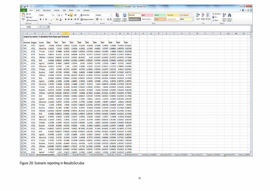
Each worksheet of file ResultsScn.xlsx contains an Excel pivot table with reported values of percent changes in macroeconomic variables relative to their base-year or baseline values for all NUTS2 regions (and all sectors where applicable), all scenarios and all years of the model horizon (see Figure 20). The title of each reported macroeconomic variable is displayed in the corresponding worksheet.

10 Depending on user needs, more of the variables computed by the model can be displayed and exported into spreadsheets, aggregating them by geographic region, economic sector and simulation year.

32

Figure 20: Scenario reporting in ResultsScn.xlsx

33

Apart from the macroeconomic indicators, we reconstruct all regional SAMs in file ReconstructedSAMs.csv, which contains the reconstructed aggregated SAMs in the comma-delimited format (.csv) that are reported for each region, each year (in case of dynamic simulations) and for each model scenario, including the baseline (BAU) case. They can be conveniently viewed in Excel, as displayed in Table 1.

Table 1: Reconstructed SAM of UKN0 region for 2012, BAU.

BAU 2012 UKN0

--- Agricul Manu Con TrTrade BusServ OthServ RnD Kap Lab_L Lab_M Lab_H Lab RnD Tax

Lab_L Tax

Lab_M Tax

Lab_H Tax-Prod

House-holds

Govern-ment

Investor Exp-EU Exp-RoW

Agricul 62.9 277.6 27.2 59.3 11.6 489.5 0.0 27.7 131.9 236.3

ManuCon 176.8 9119.4 1674.3 2075.7 2365.4 11081 0.0 4631.0 1705.5 5506.2

TrTrade 150.5 6974.0 1734.8 1077.1 501.5 1974.8 0.0 41.5 76.5 505.5

BusServ 60.1 1729.1 2389.9 5401.5 2159.4 8852.5 0.0 923.6 204.5 2641.6

OthServ 11.2 149.5 175.6 528.3 2225.7 3286.0 9044.9 117.6 73.9 259.3

RnD 3.7 109.2 142.0 430.1 191.1

Kap 281.4 2641.6 1545.4 7531.9 1258.9

Lab_L 29.3 641.1 838.1 650.7 479.9

Lab_M 40.4 1773.8 1782.0 1708.3 1614.9

Lab_H 27.4 1330.2 1035.5 1711.0 3276.7

Lab_RnD 876.0

Tax-Lab_L 6.1 134.2 175.5 136.2 100.5

Tax-Lab_M 8.5 371.4 373.1 357.7 338.1

Tax-Lab_H 5.7 278.5 216.8 541.6 686.0

Tax-prod -72.4 3147.4 450.6 928.3 322.5

Households 12847 2639.2 6919.4 7380.7 876.0 6696.0 -211.5

Government 411.4 552.6 1448.7 1728.7 4776.4 6030.5

Savings 5432.4 -792.5 3983.5 -2882.1

Imp-EU 426.0 5332.5 131.9 119.4 166.0

Imp-RoW 106.3 4326.8 343.3 1105.0 173.9

34

4.3.5 Step 5 - Sensitivity analysis

The RHOMOLO model or its individual modules can be executed from batch scripts, which is a convenient option to automate running sequences of programs or repeatable tasks, for interfacing different software or for embedding different programming languages.

In RHOMOLO, we create batch scripts every time when we have to run the same GAMS program many times, as for example to:

- import the country or regional SAMs into GAMS; - run a routine for balancing country and/or regional data; - execute RHOMOLO for different combinations of structural parameters in order to conduct

sensitivity analysis; - run the model 267 times (the number of regions in RHOMOLO) by shocking one region at a time

and analysing spatial spillover effects of a policy intervention;

- run RHOMOLO many times by varying the magnitude of the shock.

All model settings that are specified with control variables in the GAMS code can be conveniently reset in the MS-DOS script, without changing them in file RunRHOMOLO.gms.

In order to execute a GAMS task from a batch file, a user has to provide path to the model directory (e.g. cd "H:\My Documents\RHOMOLO") and to the location of gams.exe (e.g. SET GAMS="C:\GAMS\win64\24.4\gams.exe"). Later in the batch code we use "%GAMS%" to get the full path to gams.exe. The command line "%GAMS% RunRHOMOLO.gms" calls gams.exe to execute RunRHOMOLO.gms. All model settings that were specified with control variables in file RunRHOMOLO.gms (see Figure 10 in section 4.2) can be reset in the MS-DOS script by using an option symbol "--" before a control variable. When "lo=2" is declared, the batch file provides the standard output with log files and listing files. An example of batch script to run RHOMOLO (RunRHOMOLO.cmd) is shown below:

SET GAMS="C:\GAMS\win64\24.4\gams.exe"

cd "H:\My Documents\RHOMOLO"

%GAMS% RunRHOMOLO.gms --CRTS=YES --FlexibleWages=NO --DynamicPolicyShocks=YES ^

--ModelHorizon="2010*2022" --RunSCEN="/BAU,INFR/" lo=2

If the PATH environmental variable for GAMS is already set in the computer operating system, the batch file to run RHOMOLO can be simplified as follows:

cd "H:\My Documents\RHOMOLO"

GAMS RunRHOMOLO.gms --CRTS=YES --FlexibleWages=NO --DynamicPolicyShocks=YES ^

--ModelHorizon="2010*2022" --RunSCEN="/BAU,INFR/" lo=2

In order to test the influence of structural parameter values on the results of RHOMOLO simulations, sensitivity analysis is performed by running RHOMOLO for different combinations of model parameters. Among others, the following structural parameters are investigated in the sensitivity analysis:

The elasticity of substitution between different labour skill groups, 𝜎𝑅,𝑠𝐿𝑎𝑏 = 1.5 in the baseline,

ranges from 1.0 to 2.0 in the sensitivity analysis, which is a range typically observed in the empirical literature on substitution elasticities;

35

The elasticity of substitution between Labour aggregate and Capital, σr,sQ = 1.0 in the baseline,

ranges between 0.5 and 1.5 in the sensitivity analysis;

The elasticity of substitution between primary factors and intermediate inputs, σr,sZ = 0.2 in the

baseline, ranges between 0.15 and 0.25 in the sensitivity analysis;

The elasticity of substitution between different intermediate goods, σr,sX = 0.25 in the baseline,

ranges between 0.15 and 0.35 in the sensitivity analysis;

The elasticity of substitution between goods from different regions, σr,sArm = 6.0 in the baseline,

ranges between 4.0 and 8.0 in the sensitivity analysis;

The elasticity of substitution between consumer goods, σrConHou

= 1.5 in the baseline, ranges

between 1.0 and 2.0 in the sensitivity analysis;

The elasticity of substitution between investment goods, σrInv = 1.3 in the baseline, ranges between

1.0 and 1.6 in the sensitivity analysis;

The elasticity of substitution between government consumption items, σrConGov

= 0.3 in the

baseline, ranges between 0.2 and 0.4 in the sensitivity analysis.

We use control variables to define the initial value, the step size and the range of possible values of all elasticities. The elasticity parameters used for calibration of cost functions in CalibrateRHOMOLO.gms are set by the corresponding control variables defined in the batch files.

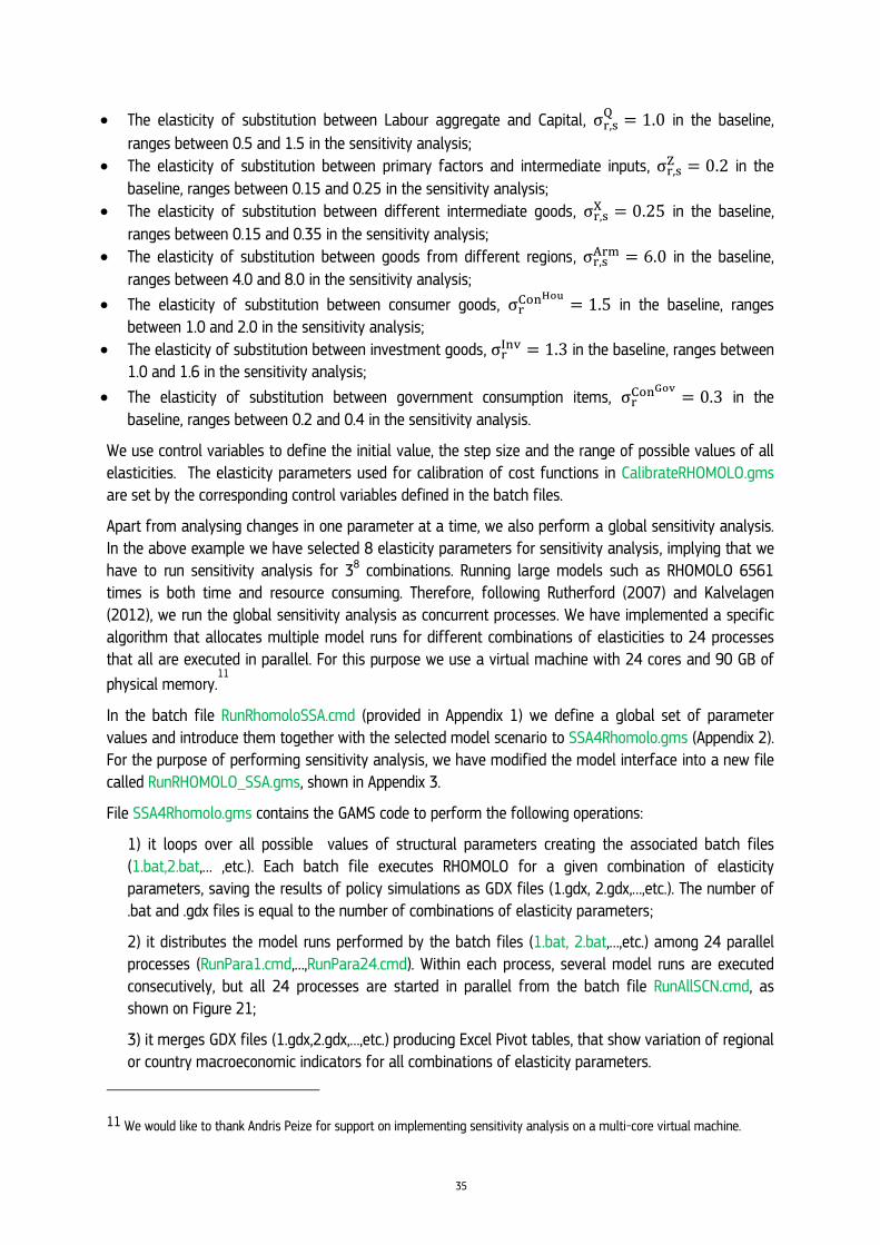
Apart from analysing changes in one parameter at a time, we also perform a global sensitivity analysis. In the above example we have selected 8 elasticity parameters for sensitivity analysis, implying that we have to run sensitivity analysis for 38 combinations. Running large models such as RHOMOLO 6561 times is both time and resource consuming. Therefore, following Rutherford (2007) and Kalvelagen (2012), we run the global sensitivity analysis as concurrent processes. We have implemented a specific algorithm that allocates multiple model runs for different combinations of elasticities to 24 processes that all are executed in parallel. For this purpose we use a virtual machine with 24 cores and 90 GB of

physical memory.11

In the batch file RunRhomoloSSA.cmd (provided in Appendix 1) we define a global set of parameter values and introduce them together with the selected model scenario to SSA4Rhomolo.gms (Appendix 2).

For the purpose of performing sensitivity analysis, we have modified the model interface into a new file called RunRHOMOLO_SSA.gms, shown in Appendix 3.

File SSA4Rhomolo.gms contains the GAMS code to perform the following operations:

1) it loops over all possible values of structural parameters creating the associated batch files (1.bat,2.bat,… ,etc.). Each batch file executes RHOMOLO for a given combination of elasticity parameters, saving the results of policy simulations as GDX files (1.gdx, 2.gdx,…,etc.). The number of .bat and .gdx files is equal to the number of combinations of elasticity parameters;

2) it distributes the model runs performed by the batch files (1.bat, 2.bat,…,etc.) among 24 parallel

processes (RunPara1.cmd,…,RunPara24.cmd). Within each process, several model runs are executed consecutively, but all 24 processes are started in parallel from the batch file RunAllSCN.cmd, as shown on Figure 21;

3) it merges GDX files (1.gdx,2.gdx,…,etc.) producing Excel Pivot tables, that show variation of regional or country macroeconomic indicators for all combinations of elasticity parameters.

11 We would like to thank Andris Peize for support on implementing sensitivity analysis on a multi-core virtual machine.

36

Figure 21: Performing sensitivity analysis with RHOMOLO by running 24 parallel processes on a 24-core processor

The batch and GAMS codes created to perform the sensitivity analysis are provided in the Appendix. Optionally, sensitivity analysis can be run either consecutively, if a line "FOR %%F IN (%TempDir%\*.bat) DO (call %%F)" is activated and a line "call %TempDir%\runAllSCN.cmd" is deactivated, or concurrently, according to the currently active settings in file RunRhomoloSSA.cmd (as shown in Appendix 1). Given that MS-DOS deals only with integers, the values of all elasticities that are set in batch files were multiplied by 1000, and then in file CalibrateRHOMOLO.gms they were consecutively divided by 1000.

The results of the sensitivity analysis are used to identify which assumptions affect most critically the results of policy simulations with RHOMOLO. In addition, they allow us to construct a ‘confidence interval’ around the policy simulation results.

As an example of sensitivity analysis with RHOMOLO, we provide an Excel sheet which shows the

variation of regional production for a 27 combinations of 3 elasticity parameters 𝜎𝑟,𝑠𝑍 , 𝜎𝑟,𝑠

𝑄 , 𝜎𝑟,𝑠𝑋 (in

GAMS notation they are Sig_ZS, Sig_ZS, and Sig_XS, correspondingly), keeping the values of other elasticities constant, as shown on Figure 22.

37

Figure 22: Results of sensitivity tests for different values of elasticities 𝜎𝑟,𝑠𝑍 , 𝜎𝑟,𝑠

𝑄 and 𝜎𝑟,𝑠𝑋 .

38

5 CONCLUDING REMARKS

RHOMOLO is the dynamic spatial general equilibrium model of the European Commission that provides sector-, region- and time-specific simulation results to support EU policy makers on structural reforms, human capital, R&D, innovation, infrastructure investments and other policies. The current version of RHOMOLO contains 267 NUTS2 regions of the EU27 Member States and each regional economy is disaggregated into six NACE Rev. 1.1 industries (agriculture; manufacturing and construction; business services; financial services; public services; and R&D). Goods and services are produced in markets that can be perfectly or imperfectly competitive to be consumed by households, government and firms. Spatial interactions between regions are captured by trade matrices, factor mobility and knowledge spill-overs, which make RHOMOLO particularly well suited for analysing policies related to human capital, transport infrastructure, R&D and innovation.

In this manual, we have presented two ways of performing simulations with the RHOMOLO model, using

either a GAMS-IDE interface or a graphical web interface. The two methods trade off complexity and flexibility, thus having advantages and disadvantages.

The main advantage of using the GAMS-IDE interface is the possibility to modify the model’s code (this

is not possible form the web interface). The IDE also facilitates the selection of specific features such as GAMS solvers, solving options, pages with syntax highlights and licences. In addition, GAMS-IDE offers many alternative options for running the model, implementing policy shocks and analysing the results of policy simulations. However, using the GAMS-IDE requires thorough knowledge of the GAMS software and syntax, and detailed understanding of the mathematical structure of the RHOMOLO model. Therefore, most users may find the graphical web interface more convenient for learning and executing the RHOMOLO model for simple/illustrative policy simulations.

The key advantage of using the web interface is that the impact of simple policy shocks can be

simulated without advanced knowledge of the GAMS software or practical CGE modelling experience. However, using the web-interface has limits in the number of possibilities/options for running the model, implementing policy shocks and tracing simulation results. Moreover, the graphical web interface is designed for learning about the RHOMOLO model and getting an idea of the output that RHOMOLO can produce, rather than for real policy simulations and impact assessment. Therefore, the choice of which simulation method to follow should be left to the user, depending on her level of software experience, specific policy needs and time availability.

As any large scale macro-economic model, RHOMOLO is a constant "work in progress", where the availability of new data, improved theoretical foundations, new evidence or better estimates of exogenous parameters, more efficient and precise solvers are always associated with incremental improvements. Hence is should be kept in mind that this manual is based on the current state of the art of the model and it can serve as a reference for the future versions, but it is still possible that small

changes will appear in the future in codes and batch files presented.

39

6 REFERENCES

Aghion, P. and P. Howitt, (1992). "A model of growth through creative destruction," Econometrica 60, 323–351.

Baldwin, R., Forslid, R., Martin, P., Ottaviano, G. and Robert-Nicoud, F. (2011). Economic Geography and Public Policy. Princeton University Press.

Blanchflower, D. G., and Oswald, A. J. (1989). The wage curve, Working Paper No. w3181. National Bureau of Economic Research.

Boeters, S., and Savard, L. (2013). The Labour Market in Computable General Equilibrium Models. Handbook of Computable General Equilibrium Modeling, 1, 1645-1718.

Brandsma, A., Kancs, D. and D. Persyn (2014). "Modelling Migration and Regional Labour Markets: An Application of the New Economic Geography Model RHOMOLO," Journal of Economic Integration, 29 (2),

249-271.

Brandsma, A., Kancs, D., Monfort, P. and A. Rillaers (2015). "RHOMOLO: A dynamic spatial general equilibrium model for assessing the impact of cohesion policy," Papers in Regional Science, 94, 197-221.

Brandsma, A. and D. Kancs (2015). "RHOMOLO: A Dynamic General Equilibrium Modelling Approach to the Evaluation of the EU's R&D Policies," Regional Studies, 49, 8, 1340–1359.

Chambers, Robert G. (1988). Applied production analysis: a dual approach. Cambridge University Press.

Di Comite, F. and Kancs, D. (2014). Modelling of Agglomeration and Dispersion in RHOMOLO. IPTS Working Papers JRC81349, European Commission, DG Joint Research Centre.

Diao, X., Roe, T. and E. Yeldan (1999). "Strategic policies and growth: an applied model of R&D-driven endogenous growth," Journal of Development Economics. 60, 343–380.

Dixit, A. K., and Stiglitz, J. E. (1977). "Monopolistic competition and optimum product diversity," The American Economic Review, 297-308.

Goulder, L.H. and S.H. Schneider (1999). "Induced technological change and the attractiveness of CO2 abatement policies," Resource and Energy Economics, 21, 211–253.

Grossman, G.M. and E. Helpman (1991). "Innovation and Growth in the Global Economy," The MIT Press, Cambridge.

Kalvelagen E. (2012). Parallel GAMS jobs, http://yetanothermathprogrammingconsultant.blogspot.com.es/ 2012/04/parallel-gamsjobs.html

Kancs, D. and B. Siliverstovs (2016), "R&D and Non-linear Productivity Growth," Research Policy, 45, 634–646.

Leahy, D. and J. P. Neary (2007). "Absorptive capacity, R&D spillovers, and public policy," International Journal of Industrial Organization, 25(5): 1089-1108.

Mansur, A. and J. Whalley (1983). Numerical Specification of Applied General Equilibrium Models: Estimation, Calibration and Data, in H. Scarf and J. Shoven (eds.), Applied General Equilibrium Analysis, Cambridge: Cambridge University Press, 69-127

Marshall, A. (1920). "Principles of economics," London: Macmillan.

40

Marzinotto, B. (2012) The growth effects of EU cohesion policy: a meta-analysis. Bruegel Working Paper

2012/14, Brussels.

Mercenier, J. (1995). Nonuniqueness of solutions in applied general equilibrium models with scale economies and imperfect competition. Economic Theory, 6(1), 161-177.

Mercenier, J., Di Comite F., Diukanova O., Kancs D. and Lopez Cobo M. (2016) RHOMOLO Model Description. IPTS Working Papers JRC100011, European Commission, DG Joint Research Centre.

Nelson, R.R. (1959). "The simple economics of basic scientific research," Journal of Political Economy, 67, 297-306.

Pyatt, G. and J.I. Round (1979) "Accounting and Fixed Price Multipliers in a Social Accounting Matrix Framework," Economic Journal 89(356): 850-73.

Romer, P. (1990). "Endogenous Technological Change," Journal of Political Economy, 98:5, 71-102.

Rutherford T. F. (2007). Programming Tools for Systematic Sensitivity Analysis of GAMS Models, http://www.mpsge.org/qtool/

Sancho, F. (2009). Calibration of CES functions for real-world multisectoral modeling. Economic Systems Research, 21(1), 45-58.

Shoven, J. and J. Whalley (1984), "Applied General-Equilibrium Models of Taxation and International Trade: An Introduction and Survey," Journal of Economic Literature, XXII, 1007-1051.

Shoven, J. and J. Whalley (1992), Applying General Equilibrium, Cambridge: Cambridge U. Press.

Thissen, M., Di Comite, F., Kancs, d. and Potters, L. (2014). Modelling Inter-Regional Trade Flows: Data and Methodological Issues in RHOMOLO. REGIO Working Papers 02/2014, European Commission, DG Regional and Urban Policy.

41

7 APPENDICES

7.1 Appendix 1. Content of the batch script RunAllSCN.cmd to run sensitivity analysis for

different combinations of model elasticity parameters

cd "H:\My Documents\IPTSmodels\RHOMOLO-Nov_8_2015VM" set SSADir=SSA_ set TempDir=%SSADir%\Temporary_SSA set PivotDir=%SSADir%\PivotTables_SSA if not exist %TempDir%\nul mkdir %TempDir% if not exist %PivotDir%\nul mkdir %PivotDir% FOR %%A IN (%TempDir%\* ) DO DEL %%A FOR %%A IN (%PivotDir%\*) DO DEL %%A set RunSCEN="/TFP_/" GAMS "%~dp0SSA4Rhomolo.gms" --SSA=YES --DynamicPolicyShocks=NO --RunSCEN=%RunSCEN% ^ --S_ZS="/150,200,250/" --S_XS="/125,250,375/" --S_QS="/500,1000,1500/" --S_LabS="/1500/" ^ --S_ArmS="/6000/" --S_Inv="/1300/" --S_ConGov="/300/" --S_ConHou="/1500/" lo=2 if exist SSA4Rhomolo.log move SSA4Rhomolo.log %TempDir%\SSA4Rhomolo.log if exist SSA4Rhomolo.lst move SSA4Rhomolo.lst %TempDir%\SSA4Rhomolo.lst if errorlevel 0 goto Step1 if errorlevel 1 goto Error :Step1 REM: run model consequitevely for all combination of elasticities ::FOR %%F IN (%TempDir%\*.bat) DO ( call %%F ) REM: run model concurrently for all combination of elasticities call %TempDir%\runAllSCN.cmd if errorlevel 0 goto Step2 if errorlevel 1 goto Error :Step2 GAMS %PivotDir%\Pivot_SSA.gms lo=2 if exist Pivot_SSA.log move Pivot_SSA.log %PivotDir%\Pivot_SSA.log if exist Pivot_SSA.lst move Pivot_SSA.lst %PivotDir%\Pivot_SSA.lst if errorlevel 1 goto Error if errorlevel 0 goto NoErrors goto END :NoErrors echo Ran Successfully ! goto END :Error echo Look for a mistake ! :END

42

7.2 Appendix 2. Content of file RunRhomolo_SSA.gms that loops over all possible values of

elasticity parameters, allocates model runs to 24 parallel processes on 24 CPU and

merges results into Excel Pivot tables

$if not set SSADir $set SSADir SSA $if not set TempDir $set TempDir %SSADir%\Temporary_SSA $if not set PivotDir $set PivotDir %SSADir%\PivotTables_SSA $if not set ActiveRun $set ActiveRun 0 $if not set DynamicPolicyShocks $set DynamicPolicyShocks NO SETS $if set S_ZS S_ZS %S_ZS% $if set S_XS S_XS %S_XS% $if set S_QS S_QS %S_QS% $if set S_LabS S_LabS %S_LabS% $if set S_ArmS S_ArmS %S_ArmS% $if set S_Inv S_Inv %S_Inv% $if set S_ConGov S_ConGov %S_ConGov% $if set S_ConHou S_ConHou %S_ConHou% display S_ZS, S_XS, S_QS, S_LabS, S_ArmS, S_Inv, S_ConGov, S_ConHou; parameter j counter of combinations; j =0 ; file ibat ; ibat.nd=0; ibat.lw=0; ibat.nw=0; put ibat; loop( (S_ZS, S_XS, S_QS, S_LabS, S_ArmS, S_Inv, S_ConGov, S_ConHou), j=j+1; put_utility 'ren' / '%TempDir%':0 '/':0 j:0 '.bat':0 ; put ibat, 'title Now processing the case ',j,' '//; put ibat, 'GAMS %SSADir%\RunRHOMOLO_SSA.gms ' put ibat, ' --SSA=YES --ActiveRun=',j,' --RunSCEN=%RunSCEN% ' put ibat, ' --S_ZS=',S_ZS.tl,' --S_XS=',S_XS.tl,' --S_QS=',S_QS.tl,' --S_LabS=',S_LabS.tl, put ibat, ' --S_ArmS=',S_ArmS.tl,' --S_Inv=',S_Inv.tl,' --S_ConGov=',S_ConGov.tl,' --S_ConHou=',S_ConHou.tl, put ibat, ' o=%TempDir%\',j,'.lst ' ; ); putclose ibat display j; $Eval NuRuns card(S_ZS)*card(S_XS)*card(S_QS)*card(S_LabS)*card(S_ArmS)*card(S_Inv)*card(S_ConGov)*card(S_ConHou) * *Run concurrently : set cjob concurrent processes : equal to the number of CPUs /cjob1*cjob24/, jj number of all combinations /1*%NuRuns%/, assign (cjob,jj); loop( (cjob,jj), assign(cjob,jj)$[ ( ord(jj) le {card(jj)/card(cjob)}*ord(cjob) ) and ( ord(jj) gt {card(jj)/card(cjob)}*{ord(cjob) -1} ) ]= YES ; ); display assign, jj ; abort$sum(jj, abs(sum(assign(cjob,jj),1)-1) ) "jobs are not correctly assigned"; file f ; f.nd=0; f.lw=0; f.nw=0; file g /'%TempDir%\runAllSCN.cmd'/; loop(cjob, put f, put_utility 'ren'/ '%TempDir%':0 '/':0 'RunPara',ord(cjob):0:0,'.cmd'; loop( assign(cjob,jj), put f, "call %TempDir%\", ord(jj):0:0,'.bat'/; ); putclose f, "EXIT" /; put g, 'start %TempDir%\','RunPara', ord(cjob):0:0,'.cmd' /; );

43

put g, ' timeout /t 7200 '/; putclose g, "EXIT /B"; **Merge the results of all model runs and produce pivot tables file Pivoting /%PivotDir%\Pivot_SSA.gms/; put Pivoting ; $onputS $if not set SSADir $set SSADir SSA $if not set TempDir $set TempDir %SSADir%\Temporary_SSA $if not set PivotDir $set PivotDir %SSADir%\PivotTables_SSA $show **since domains are lost during merging we re-initialize them $set SCN SCN alias (*,%SCN%); $set DIMENS Reg,TT alias (*,%DIMENS%); $set elasticities S_ZS,S_XS,S_QS,S_LabS,S_ArmS,S_Inv,S_ConGov,S_ConHou alias (*,%elasticities%); $call 'gdxmerge %TempDir%\*.gdx id=elas_combi,rGDPexp_V,Toutput_V,HHCons_V,rGDP,Toutput,HHCons, ' $gdxin merged.gdx set Merged_set_1; $load Merged_set_1 = Merged_set_1 set elas_combi1(Merged_set_1,%elasticities%); $load elas_combi1 =elas_combi **2 restore the domains : parameter rGDPexp_V( Merged_set_1, %SCN%, %DIMENS% ) $load rGDPexp_V parameter rGDP( Merged_set_1, %SCN%, %DIMENS% ) $load rGDP parameter Toutput_V( Merged_set_1, %SCN%, %DIMENS% ) $load Toutput_V parameter Toutput( Merged_set_1, %SCN%, %DIMENS% ) $load Toutput Parameter HHCons_V( Merged_set_1, %SCN%, %DIMENS% ) $load HHCons_V parameter HHCons( Merged_set_1, %SCN%, %DIMENS%) $load HHCons $gdxin display Merged_set_1, elas_combi1, rGDPexp_V, Toutput_V, HHCons_V, rGDP, Toutput, HHCons; $call 'if exist merged.gdx move merged.gdx %PivotDir%\merged.gdx' parameters rGDPexp_V2( Merged_set_1, %SCN%, %elasticities%, Reg ), rGDP_2( Merged_set_1, %SCN%, %elasticities%, Reg ), Toutput_V2( Merged_set_1, %SCN%, %elasticities%, Reg ), Toutput_2( Merged_set_1, %SCN%, %elasticities%, Reg ), HHCons_V2( Merged_set_1, %SCN%, %elasticities%, Reg ), HHCons_2( Merged_set_1, %SCN%, %elasticities%, Reg ) ; loop( elas_combi1( Merged_set_1, %elasticities% ), rGDPexp_V2( Merged_set_1, %SCN%, %elasticities%, Reg ) = rGDPexp_V( Merged_set_1, %SCN%, Reg, "2010" ); Toutput_V2( Merged_set_1, %SCN%, %elasticities%, Reg ) = Toutput_V( Merged_set_1, %SCN%, Reg, "2010" ); HHCons_V2( Merged_set_1, %SCN%, %elasticities%, Reg ) = HHCons_V( Merged_set_1, %SCN%, Reg, "2010" ); rGDP_2( Merged_set_1, %SCN%, %elasticities%, Reg ) = rGDP( Merged_set_1, %SCN%, Reg, "2010" ); Toutput_2( Merged_set_1, %SCN%, %elasticities%, Reg ) = Toutput( Merged_set_1, %SCN%, Reg, "2010" ); HHCons_2( Merged_set_1, %SCN%, %elasticities%, Reg ) = HHCons( Merged_set_1, %SCN%, Reg, "2010" ); ); display rGDPexp_V2, Toutput_V2, HHCons_V2, rGDP_2, Toutput_2, HHCons_2; $set AllElasticities Sig_ZS,Sig_XS,Sig_QS,Sig_LabS,Sig_ArmS,Sig_Inv,Sig_ConGov,Sig_ConHou set Header /"Number of Similation","Model Scenario",%AllElasticities%/; display Header ; execute_unload '%PivotDir%\PivotTables.gdx', Header, rGDPexp_V2, Toutput_V2, HHCons_V2,rGDP_2, Toutput_2, HHCons_2; $onecho >gdxxrw.rsp

44

set=Header rng="GDPreal_value!a2" values=nodata rdim=0 cdim=1 par=rGDPexp_V2 rng="GDPreal_value!a3" rdim=10 cdim=1 set=Header rng="GDPrealVS2010!a2" values=nodata rdim=0 cdim=1 par=rGDP_2 rng="GDPrealVS2010!a3" rdim=10 cdim=1 set=Header rng="Production_value!a2" values=nodata rdim=0 cdim=1 par=Toutput_V2 rng="Production_value!a3" rdim=10 cdim=1 set=Header rng="ProductionVS2010!a2" values=nodata rdim=0 cdim=1 par=Toutput_2 rng="ProductionVS2010!a3" rdim=10 cdim=1 set=Header rng="HouseHoldConsumption_value!a2" values=nodata rdim=0 cdim=1 par=HHcons_V2 rng="HouseHoldConsumption_value!a3" rdim=10 cdim=1 set=Header rng="HouseHoldConsumptionVS2010!a2" values=nodata rdim=0 cdim=1 par=HHcons_2 rng="HouseHoldConsumptionVS2010!a3" rdim=10 cdim=1 $offecho execute 'gdxxrw i=%PivotDir%\PivotTables.gdx o=%PivotDir%\PivotTables.xlsx @gdxxrw.rsp'; execute 'gdxxrw i=%PivotDir%\PivotTables.gdx o=%PivotDir%\PivotTables.xlsx text="Elasticities:" rng=GDPreal_value!c1' execute 'gdxxrw i=%PivotDir%\PivotTables.gdx o=%PivotDir%\PivotTables.xlsx text="real GDP: values" rng=GDPreal_value!k1' execute 'gdxxrw i=%PivotDir%\PivotTables.gdx o=%PivotDir%\PivotTables.xlsx text="Elasticities:" rng=GDPrealVS2010!c1' execute 'gdxxrw i=%PivotDir%\PivotTables.gdx o=%PivotDir%\PivotTables.xlsx text="real GDP: % deviation from base year values" rng=GDPrealVS2010!k1' execute 'gdxxrw i=%PivotDir%\PivotTables.gdx o=%PivotDir%\PivotTables.xlsx text="Elasticities:" rng=Production_value!c1' execute 'gdxxrw i=%PivotDir%\PivotTables.gdx o=%PivotDir%\PivotTables.xlsx text="cumulative output: values" rng=Production_value!k1' execute 'gdxxrw i=%PivotDir%\PivotTables.gdx o=%PivotDir%\PivotTables.xlsx text="Elasticities:" rng=ProductionVS2010!c1' execute 'gdxxrw i=%PivotDir%\PivotTables.gdx o=%PivotDir%\PivotTables.xlsx text="cumulative output: % deviation from base year values" rng=ProductionVS2010!k1' execute 'gdxxrw i=%PivotDir%\PivotTables.gdx o=%PivotDir%\PivotTables.xlsx text="Elasticities:" rng=HouseHoldConsumption_value!c1' execute 'gdxxrw i=%PivotDir%\PivotTables.gdx o=%PivotDir%\PivotTables.xlsx text="household consumption: values" rng=HouseHoldConsumption_value!k1' execute 'gdxxrw i=%PivotDir%\PivotTables.gdx o=%PivotDir%\PivotTables.xlsx text="Elasticities:" rng=HouseHoldConsumptionVS2010!c1' execute 'gdxxrw i=%PivotDir%\PivotTables.gdx o=%PivotDir%\PivotTables.xlsx text="household consumption: % deviation from base year values" rng=HouseHoldConsumptionVS2010!k1' EXECUTE '=shellexecute %PivotDir%\PivotTables.xlsx'; $offput putclose Pivoting; $show

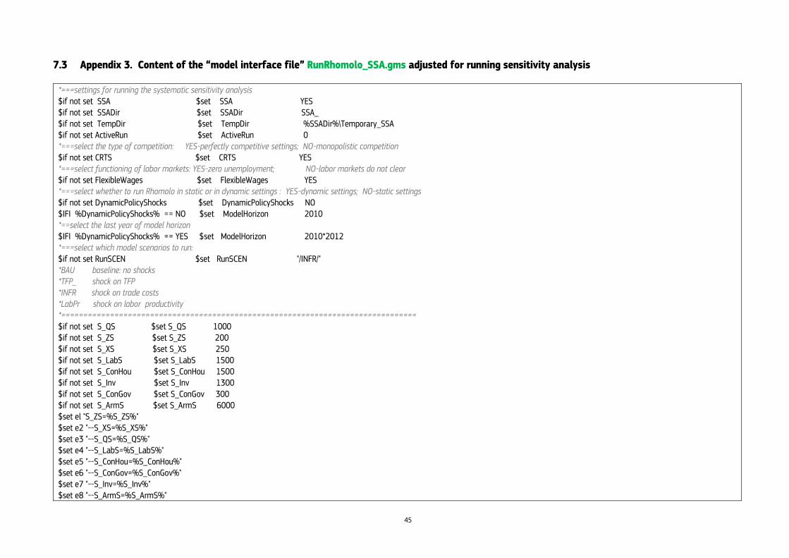
45

7.3 Appendix 3. Content of the “model interface file” RunRhomolo_SSA.gms adjusted for running sensitivity analysis

*===settings for running the systematic sensitivity analysis $if not set SSA $set SSA YES $if not set SSADir $set SSADir SSA_ $if not set TempDir $set TempDir %SSADir%\Temporary_SSA $if not set ActiveRun $set ActiveRun 0 *===select the type of competition: YES-perfectly competitive settings; NO-monopolistic competition $if not set CRTS $set CRTS YES *===select functioning of labor markets: YES-zero unemployment; NO-labor markets do not clear $if not set FlexibleWages $set FlexibleWages YES *===select whether to run Rhomolo in static or in dynamic settings : YES-dynamic settings; NO-static settings $if not set DynamicPolicyShocks $set DynamicPolicyShocks NO $IFI %DynamicPolicyShocks% == NO $set ModelHorizon 2010 *==select the last year of model horizon $IFI %DynamicPolicyShocks% == YES $set ModelHorizon 2010*2012 *===select which model scenarios to run: $if not set RunSCEN $set RunSCEN "/INFR/" *BAU baseline: no shocks *TFP_ shock on TFP *INFR shock on trade costs *LabPr shock on labor productivity*================================================================================$if not set S_QS $set S_QS 1000 $if not set S_ZS $set S_ZS 200 $if not set S_XS $set S_XS 250 $if not set S_LabS $set S_LabS 1500 $if not set S_ConHou $set S_ConHou 1500 $if not set S_Inv $set S_Inv 1300 $if not set S_ConGov $set S_ConGov 300 $if not set S_ArmS $set S_ArmS 6000 $set el "S_ZS=%S_ZS%"$set e2 "--S_XS=%S_XS%"$set e3 "--S_QS=%S_QS%"$set e4 "--S_LabS=%S_LabS%"$set e5 "--S_ConHou=%S_ConHou%"$set e6 "--S_ConGov=%S_ConGov%"$set e7 "--S_Inv=%S_Inv%"$set e8 "--S_ArmS=%S_ArmS%"

46

$set AllElasticities "%el% %e2% %e3% %e4% %e5% %e6% %e7% %e8%" $show *=============================================================================== $setglobal IDE "IDE=%GAMS.ide% lo=%GAMS.lo% errorlog=%GAMS.errorlog% errmsg=1" $set d1 "-DynamicPolicyShocks=%DynamicPolicyShocks%" $set d2 "--ModelHorizon=%ModelHorizon%" $set Horizon "%d1% %d2%" *=============================================================================== $if not set DataReadRegionalization $set DataReadRegionalization NO $IFI %DataReadRegionalization% == YES EXECUTE 'GAMS AggregateCntSAMs.gms S=.\SaveRestart\AggregateCntSAMs %IDE%' ; $IFI %DataReadRegionalization% == YES EXECUTE 'GAMS AggregateRegBiTradeMatrix.gms R=.\SaveRestart\AggregateCntSAMs S=.\SaveRestart\AggregateRegBiTradeMatrix %IDE%' ; $IFI %DataReadRegionalization% == YES EXECUTE 'GAMS CompileRegSams.gms R=.\SaveRestart\AggregateRegBiTradeMatrix S=.\SaveRestart\CompileRegSams %IDE%' ; $IFI %SSA% == YES EXECUTE 'GAMS CalibrateRHOMOLO.gms R=.\SaveRestart\CompileRegSams S=.\SaveRestart\CalibrateRHOMOLO%ActiveRun% --CRTS=%CRTS% --FlexibleWages=%FlexibleWages% --%AllElasticities% %IDE% ' ;

$IFI %SSA% == NO EXECUTE 'GAMS CalibrateRHOMOLO.gms R=.\SaveRestart\CompileRegSams S=.\SaveRestart\CalibrateRHOMOLO --CRTS=%CRTS% --FlexibleWages=%FlexibleWages% %IDE% ' ; *run the core model to reproduce the benchmark situation of 2010EXECUTE 'GAMS RHOMOLO_Equations.gms R=.\SaveRestart\CalibrateRHOMOLO%ActiveRun% S=.\SaveRestart\RHOMOLO_Equations%ActiveRun% %IDE%' ; *Run counterfactual scenarios :$IFI %SSA% == YESEXECUTE 'GAMS RunCounterfactualScenarios.gms R=.\SaveRestart\RHOMOLO_Equations%ActiveRun% --%Horizon% --RunSCEN="%RunSCEN%" GDX=%TempDir%\%ActiveRun% %IDE%' ; $IFI %SSA% == NOEXECUTE 'GAMS RunCounterfactualScenarios.gms R=.\SaveRestart\RHOMOLO_Equations --%Horizon% S=.\SaveRestart\RunCounterfactualScenarios %IDE%' ; *Send results of RHOMOLO simulations to Excel:$IFI %SSA% == NOEXECUTE 'GAMS SendResults2Excel.gms R=.\SaveRestart\RunCounterfactualScenarios %IDE%' ;

47

Europe Direct is a service to help you find answers to your questions about the European Union

Freephone number (*): 00 800 6 7 8 9 10 11

(*) Certain mobile telephone operators do not allow access to 00 800 numbers or these calls may be billed.

A great deal of additional information on the European Union is available on the Internet.

It can be accessed through the Europa server http://europa.eu.

How to obtain EU publications

Our publications are available from EU Bookshop (http://bookshop.europa.eu),

where you can place an order with the sales agent of your choice.

The Publications Office has a worldwide network of sales agents.

You can obtain their contact details by sending a fax to (352) 29 29-42758.

European Commission

EUR 27351 EN – Joint Research Centre – Institute for Prospective Technological Studies

Title: RHOMOLO Model Manual

Author(s): Francesco Di Comite, Olga Diukanova, D'Artis Kancs

Luxembourg: Publications Office of the European Union

2015 – 46 pp. – 21.0 x 29.7 cm

EUR – Scientific and Technical Research series – ISSN 1831-9424 (online)

ISBN 978-92-79-49579-3 (PDF)

doi:10.2791/185683

48 ISBN 978-92-79-49579-3

doi:10.2791/185683

JRC Mission

As the Commission’s in-house science service, the Joint Research Centre’s mission is to provide EU policies with independent, evidence-based scientific and technical support throughout the whole policy cycle.

Working in close cooperation with policy Directorates-General, the JRC addresses key societal challenges while stimulating innovation through developing new methods, tools and standards, and sharing its know-how with the Member States, the scientific community and international partners.

Serving society Stimulating innovation Supporting legislation

LF-N

A-2

73

51

-EN

-N