ricerca di sistema elettrico - enea.it · cresco-enea grid cluster located in portici. the nurisp...
TRANSCRIPT

RICERCA DI SISTEMA ELETTRICO
Implementation and validation of the NURISP platform
F. Bassenghi, G. Bornia, L. Deon, S. Manservisi, P. Meloni, M. Polidori
Report RdS/2011/126
Agenzia Nazionale per le Nuove Tecnologie, l’Energia e lo Sviluppo Economico Sostenibile
IMPLEMENTATION AND VALIDATION OF THE NURISP PLATFORM F. Bassenghi, G. Bornia, L. Deon, S. Manservisi – Unibo Dienca, P. Meloni, M. Polidori - ENEA Settembre 2011 Report Ricerca di Sistema Elettrico Accordo di Programma Ministero dello Sviluppo Economico – ENEA Area: Governo, Gestione e sviluppo del sistema elettrico nazionale Progetto: Nuovo nucleare da fissione: collaborazioni internazionali e sviluppo competenze in materia nucleare Responsabile Progetto: Paride Meloni, ENEA

1 107
Distrib. I Pag. diSigla di identificazione
Ei'Eh.. Ricerca Sistema Elettrico NNFISS - LP5 - 020 L
Titolo
Implementation and validation of the NURISP platform
DescrittoriTipologia del documento:Collocazione contrattuale:
Rapporto TecnicoAccordo di programma ENEA-MSE: tema di ricerca "Nuovonucleare da fissione"Reattori nucleari evolutiviTermoidraulica dei reattori nucleariCodici di calcolo
Argomenti trattati:
SommarioLa piattaforma NURISP e un progetto europeo sviluppato per simulare il comportamentotermoidraulico dei componenti degli impianti nucleari e facility sperimentali. Questa piattaforma eutilizzata per analizzare situazioni fisiche a diverse scale e consiste di numerosi codici che vengonoutilizzati per generare mesh, visualizzare i risultati e risolvere equazioni che descrivono 10 stato delsistema da simulare. La piattaforma di gestione SALOME e i codici TRIO_U, NEPTUNE e CATHAREsono stati installati sui computer cluster CRESCO ENEA-GRID che si trova a Portici. TRIO_U e iIcod ice NEPTUNE risolvono Ie equazioni termoidrauliche in geometrie multidimensionali conparticolare attenzione al flusso bifase. II codice CATHARE e un codice a parametri concentrati cheviene utilizzato per studiare il comportamento dipendente dal tempo di sistemi complessi. In questarapporto sono discussi I'implementazione e la validazione della piattaforma effettuata attraverso iIconfronto con dati sperimentali. II codice NEPTUNE e validato con dati sperimentali dell'impiantoPERSEOe iI codice TRIO_U con alcuni dati sperimentali riguardanti una bolla che si stacca da paretiriscaldate. CATHARE e validato su dati sperimentali dell'impianto SPES-99.
NoteII documento e stato realizzato all'interno della collaborazione ENEA-CIRTEN (UniBo).REPORT LPS-Al - PAR 2008-2009Autori: F. BassenghP, G. Bornia(*), L. Deon(*), S. Manservisi(*), P. Meloni("), M. Polidori(**)
(*)Universita di Bologna - DIENCA (**)ENEA UTFISSM
Copia n. In carico a:
NOME2FIRMA
NOME1FIRMA
Massimiliano po~ S~~nia Baccaro
JF....A'AO~
NOME Paride Melonio EMISSIONEFIRMA ~o-vt7L' ~ - - -
REDAZIONE CONVALIDAREV. DESCRIZIONE DATA APPROVAZIONE

IMPLEMENTATION AND VALIDATION OF THENURISP PLATFORM
September 1, 2011
F. Bassenghi, G. Bornia, L. Deon and S. [email protected]
DIENCA - University of Bologna Via dei Colli 16, 40136 Bologna, Italy
P. Meloni and M. [email protected]
ENEA - Via Martiri di Monte Sole 4, 40129 Bologna, Italy
Abstract. The NURISP platform is a European project developed to simulatethe thermal-hydraulic behavior of the components of nuclear plants and facilities.This platform is used to investigate physical situations at different scales rang-ing from boiling bubbles to nuclear reactors. In this report the implementationand validation of the platform are discussed. The platform manager SALOMEand the TRIO_U, NEPTUNE and CATHARE codes have been installed on theCRESCO-ENEA GRID cluster located in Portici. The NURISP platform con-sists of many codes that are used to generate meshes, visualize results and solveequations describing the state of the system to be simulated. In this report wefocus in particular on TRIO_U, NEPTUNE and CATHARE codes. TRIO_Uand NEPTUNE codes solve the thermal-hydraulics equations in multidimensionalgeometries with particular attention to the two-phase flow. The CATHARE codeis a lumped parameter thermal-hydraulic code that is used to investigate the timedependent behavior of complex systems. Validation of the platform on experimen-tal data is reported. In this report NEPTUNE code is validated against PERSEOfacility experimental data and TRIO_U code against some experimental data in-volving bubble detaching from heating walls. CATHARE is validated on SPES-99facility experimental data.

Contents
1 NURISP platform implementation 71.1 CRESCO-ENEA GRID implementation . . . . . . . . . . . . . . . 71.2 Overview of NURISP platform codes . . . . . . . . . . . . . . . . . 10
1.2.1 SALOME . . . . . . . . . . . . . . . . . . . . . . . . . . . . 131.2.2 NEPTUNE . . . . . . . . . . . . . . . . . . . . . . . . . . . 151.2.3 TRIO_U . . . . . . . . . . . . . . . . . . . . . . . . . . . . 171.2.4 SATURNE . . . . . . . . . . . . . . . . . . . . . . . . . . . 191.2.5 CATHARE . . . . . . . . . . . . . . . . . . . . . . . . . . . 21
1.3 Platform pre- and post-processing operations . . . . . . . . . . . . . 221.3.1 Input/output formats . . . . . . . . . . . . . . . . . . . . . . 231.3.2 Mesh input files . . . . . . . . . . . . . . . . . . . . . . . . . 261.3.3 The PARAVIEW application . . . . . . . . . . . . . . . . . 29
1.4 Platform code coupling and services . . . . . . . . . . . . . . . . . . 311.4.1 SALOME clustering service system . . . . . . . . . . . . . . 311.4.2 SALOME module and code integration . . . . . . . . . . . . 321.4.3 Coupling codes inside SALOME platform . . . . . . . . . . 33
2 Validation of the CATHARE model of the SPES-99 facility 352.1 THE SPES-99 FACILITY . . . . . . . . . . . . . . . . . . . . . . . 352.2 CATHARE 2 Code and SPES-99 Model . . . . . . . . . . . . . . . 372.3 SPES-99 facility steady state . . . . . . . . . . . . . . . . . . . . . . 39
2.3.1 Steady state . . . . . . . . . . . . . . . . . . . . . . . . . . . 392.3.2 Reference steady state . . . . . . . . . . . . . . . . . . . . . 40
2.4 SPES-99 IB LOCA transient . . . . . . . . . . . . . . . . . . . . . . 432.4.1 Results of the experiment . . . . . . . . . . . . . . . . . . . 432.4.2 Comparison between post-test results and experimental data 45
3 Validation of a NEPTUNE-CATHARE model on PERSEO facil-ity 493.1 The PERSEO facility test . . . . . . . . . . . . . . . . . . . . . . . 49
3.1.1 The PERSEO facility design . . . . . . . . . . . . . . . . . . 49

CONTENTS
3.1.2 PERSEO experimental test 9 . . . . . . . . . . . . . . . . . 523.2 CATHARE-NEPTUNE coupled simulation . . . . . . . . . . . . . 543.3 Cathare solution of the PERSEO facility . . . . . . . . . . . . . . . 56
3.3.1 Cathare modeling of the PERSEO facility . . . . . . . . . . 563.3.2 Cathare solution of test n.9 . . . . . . . . . . . . . . . . . . 593.3.3 Boundary conditions for NEPTUNE . . . . . . . . . . . . . 60
3.4 NEPTUNE on CRESCO set up simulation . . . . . . . . . . . . . . 623.4.1 Code setup . . . . . . . . . . . . . . . . . . . . . . . . . . . 623.4.2 Initial, boundary condition and physical property files . . . . 64
3.5 NEPTUNE simulation of PERSEO Test 9 . . . . . . . . . . . . . . 703.5.1 Beginning of the test . . . . . . . . . . . . . . . . . . . . . . 713.5.2 Temperature stratification . . . . . . . . . . . . . . . . . . . 743.5.3 Steam injection on boiling pool . . . . . . . . . . . . . . . . 763.5.4 Injection above water level . . . . . . . . . . . . . . . . . . . 80
4 Validation of TRIO_U interface model on bubble detachment 854.1 Set up of the TRIO_U code . . . . . . . . . . . . . . . . . . . . . . 854.2 Numerical results . . . . . . . . . . . . . . . . . . . . . . . . . . . . 89
4.2.1 Simulation of bubble detachment in pool boiling . . . . . . 894.2.2 Bubble diameter as a function of gravity . . . . . . . . . . . 904.2.3 Bubble diameter as a function of surface tension . . . . . . . 954.2.4 Interface coalescence test . . . . . . . . . . . . . . . . . . . . 99
4

CONTENTS
IntroductionThis document reports some advances in the implementation, development andvalidation of the NURISP platform on the CRESCO-ENEA grid with the purposeof studying the thermal-hydraulic behavior of LWR evolutive nuclear reactors. Thedevelopment of the NURISP platform reflects the new European policy of buildinga common suite of computational tools to investigate such complex problems. TheNURISP platform project is funded by EC. ENEA is a user group member of theproject and has obtained the use of several codes under a direct agreement. TheUniversity of Bologna participates in the effort of using, installing and validatingthese computational tools and other in-house codes on the CRESCO-ENEA GRIDcluster located in Portici (near Naples).
The complexity of nuclear reactor thermal-hydraulics consists in the presence ofdifferent physical phenomena occurring at different geometrical scales. Therefore,multi-physics and multi-scale investigations arise in the study of nuclear reactorcomponents. Clearly, these models cannot be analyzed simultaneously and thecoupling between various codes is necessary to achieve an accurate and satisfactoryresult. Hence, the NURISP platform has been conceived not only to collect a seriesof codes that have been extensively used in this field but also to harmonize themwith reference input and output formats. Reference mesh and output formatsare standardized and conversion tools are developed. The aim of the platform isto solve complex problems exchanging information between different codes overlarge multiprocessor architectures. Validation of some models implemented on theplatform codes is performed by comparison with available experimental data.
In Chapter 1 we give an overview of the organization of the platform. The pur-pose of solving complex problems is discussed together with the implementation ofthe NURISP platform on CRESCO-ENEA GRID. The reference mesh and outputformats are introduced and the visualization open-source application PARAVIEWis described together with the main codes of the platform: NEPTUNE, TRIO_Uand CATHARE.
In Chapter 2 a CATHARE model of the SPES-99 facility is presented. Themodel is developed in great detail including small components and geometries.First the steady state is calibrated by using the main termohydraulic parametersin order to reproduce the real behavior of the facility as accurately as possible.This calibration with the experimental data reduces the uncertainties related to thefacility. Then the transient behavior of the SPES-99 facility for an intermediatebreak loss of coolant accident (IBLOCA) is simulated and verified against theexperimental data.
Chapter 3 reports the analysis of the computational simulation of an exper-imental test of the PERSEO facility. The experiment is simulated by couplingCATHARE and NEPTUNE codes. The facility is simulated by using the mono-
5

CONTENTS
dimensional code CATHARE and then this solution is used as a boundary condi-tion for the NEPTUNE simulation of a facility component. With the NEPTUNEcode the overall pool and the injector of the PERSEO facility are simulated andthe results are compared with the experimental data.
Finally Chapter 4 is devoted to the validation of the TRIO_U two-phase andtracking interface model. With TRIO_U we simulate the bubble detaching fromheated walls in pool boiling configuration.
6

Chapter 1
NURISP platform implementation
The NURISP platform has been implemented on the CRESCO-ENEA grid system.This implementation is part of the FISSICU platform that contains also meshgeneration and visualization tools together with other codes. In this chapter wefirst describe the CRESCO-ENEA grid system. Then we illustrate the NURISPplatform and the implementation of each code. We describe the mesh and datafile formats used by the codes and the software for their visualization. In the lastsection we discuss about the coupling between the codes that can be implementedwith the SALOME software.
1.1 CRESCO-ENEA GRID implementationCRESCO (Centro Computazionale di RicErca sui Sistemi Complessi, Computa-tional Research Center for Complex Systems) is an ENEA Project, co-funded bythe Italian Ministry of Education, University and Research (MIUR). The CRESCOproject is located in the Portici ENEA Center near Naples and consists of a HighPerformance Computing infrastructure mainly devoted to the study of ComplexSystems [10]. The CRESCO project is built around the HPC platform through thecreation of a number of scientific thematic laboratories: Computing Science Labo-ratory (CSL), Computational Systems Biology Laboratory (CSBL) and ComplexNetworks Systems Laboratory (CNSL). The Computing Science Laboratory hostsactivities on hardware and software design, GRID technology that also integratesthe HPC platform management. The Computational Systems Biology Laboratoryhosts the activities in the Life Science domain and the Complex Networks SystemsLaboratory the activities on complex technological infrastructures.
There are four ways to access ENEA-GRID:a) SSH client, with a terminal interface which can directly access to one of thefront-end machines;

NURISP platform implementation
ACCESS ACCESSCluster Node Name SSH from SSH from OSname ENEA world
Brindisi brindisi-fg1.brindisi.enea.it yes no LINUXCasaccia crescoc1.casaccia.enea.it yes no LINUXFrascati crescof01.frascati. enea.it yes no LINUX
lin4p.frascati.enea.it yes yes LINUXsp5-1.frascati.enea.it yes no AIX
Portici CRESCOcresco1-f1.portici.enea.it yes yes LINUXcresco1-f2.portici.enea.it yes no LINUXcresco1-f3.portici.enea.it yes no LINUXcresco2-f1.portici.enea.it yes no LINUXcresco2-f2.portici.enea.it yes no LINUXcresco2-f3.portici.enea.it yes no LINUXcresco1-fg1.portici.enea.it yes no LINUXcresco1-fg2.portici.enea.it yes no LINUXcresco1-fg3.portici.enea.it yes no LINUXcresco1-fg4.portici.enea.it yes no LINUXcresco-fpga6.portici.enea.it yes no LINUX
Table 1.1: CRESCO front-end machines.
b) Citrix client, that can be installed on windows machines to access ENEA servers,including a terminal window to ENEA-GRID (INFOGRID);c) FARO (Fast Access to Remote Objects) ENEA-GRID, that is a Java web in-terface available for all operating systems;d) NX client.
The access is limited to authorized users that are provided with ENEA-GRIDusername and password to be used on every machine of the grid. Table 1.1 showsa list of available nodes. There are a number of front-end nodes to access theplatform from the external world.
After the login at the web interface FARO (http://www.cresco.enea.it/nx.html), from any operating system a terminal can be used from where all theapplications can be launched. Further details on the login procedure can be foundon the CRESCO website (http://www.cresco.enea.it/helpdesk.php).
The CRESCO-ENEA GRID system hosts a platform of codes for the simulationof nuclear components and facilities called FISSICU platform, a part of which forms
8

NURISP platform implementation
the NURISP platform. FISSICU platform contains also other codes that are notdirectly related to the NURISP project. The FISSICU project is located in thedirectory
/afs/enea.it/project/fissicu
The main directory fissicu consists of three sub-directories
- data, where the simulation data should be stored;
- html, where the web pages with help are located(http://www.afs.enea.it/project/fissicu/);
- soft, where all the codes are installed.
Inside the soft directory the FISSICU project has the following installed codes
- SALOME that runs with the command salome;
- CATHARE that runs with the command cathare;
- NEPTUNE that runs with the command neptune;
- TRIO_U that runs with the command triou;
- SATURNE that runs with the command saturne;
- FEM-UNIBO (the finite element Navier-Stokes solver developed at DIENCA- University of Bologna).
For each code, a script (executable_env) is also available which simply setsthe proper environment variables to execute the code. This procedure can be usedto run the code directly without any graphical interface on a single node wherethe user is logged. This is also the first step for production runs which use thebatch queue to run the code in parallel. Any code has a script in the directory
\code{/afs/enea.it/project/fissicu/soft/bin}
that allows the program to run. This directory should be added to the user envi-ronment variable PATH. In the bash shell the command line is
$ export PATH=/afs/enea.it/project/fissicu/soft/bin:$PATH
This command line can also be added to the configuration file .bashrc.CRESCO supports the LSF (Load Sharing Facility) job scheduler, which is a
suite of several components to manage a large cluster of computers with differentarchitectures and operating systems. The basic commands are
9

NURISP platform implementation
- lshosts that displays the host information ;
- lshosts that displays the host information;
- bhosts that displays information about the hosts such as their status, thenumber of running jobs, etc.;
- bqueues that lists the available LSF batch queues and their scheduling andcontrol status;
- bsub < job.lsf that submits a job to a queue. The script job.lsf containsjob submission options as well as command lines to be executed.
- bjobs that reports the status of LSF batch jobs of the user.
- bkill JOBID that kills the job with number JOBID. This number can beretrieved with the command bjobs.
A typical script is
#!/bin/bash#BSUB -J JOBNAME#BSUB -q quename#BSUB -n nproc#BSUB -oo stdout_file#BSUB -eo errout_file#BSUB -i input_filecode_envrun_command datafile.data
where the options to BSUB specify respectively the name of the job, the name of thequeue, the number of processors, the file names for the standard and error output,the input file. The last two lines set the environment variables for the code andlaunch the executable with a parameter file, without the graphical interface thatclearly cannot be used when submitting a job with a batch queue.
1.2 Overview of NURISP platform codesThe study of nuclear reactor thermal-hydraulics involves physical phenomena ofdifferent nature (heat transfer, two-phase flow, chemical poisoning) that cannot beanalyzed in a simultaneous manner. Improvements are necessary both for phys-ical models (heat transfer coefficient at the interface between liquid and vapor,
10

NURISP platform implementation
instabilities of the interface, diffusion coefficients) and for numerical schemes (ac-curacy, CPU time). Even when experimental correlations are available for a singleequation the complexity of the problems does not allow a whole-system simula-tion. The problem can be segregated in sub-tasks but often each physical modelrequires a number of parameters that are determined by the other state variablesand the coupling between the equations is necessary to achieve an accurate andsatisfactory result. For all these reasons it is important to develop tools that cansolve in a segregated manner coupled system of equations with codes that are spe-cific for a single application. The problem of coupling codes is one of the mainissues of the NURISP platform. In the NURISP platform there are three differenttypes of coupling: weak, internal weak and strong coupling. In the first case theweak coupling is performed with the exchange of input and output files. In thiscase the file format must be shared by all the applications or external conversiontools are required. In the internal weak coupling all the equations are solved in asegregated way using memory to exchange data among them. The strong couplingis the solution of all the equations with a unique implicit and iterative algorithm.
Another aspect of the complexity of nuclear reactor simulations is the presenceof different geometrical scales. In the nuclear reactor field one needs to investigatemicro-scale, meso-scale and macro-scale problems with different characteristic di-mensions ranging from millimeters to several meters. It is not possible to solvesuch complex problems in a single simulation. Therefore the computational toolsshould be able to model different scales with different equations and take intoaccount the relevant physics for the selected geometries. The phenomena at themicro-scale level can be simulated by solving the three-dimensional Navier-Stokesequations with commercial software such as ANSYS-FLUENT, CFX and Comsolmultiphysics or with open source software such as OPENFOAM and SATURNE.In the NURISP platform the three-dimensional CFD code that solves the Navier-Stokes equation is TRIO_U. The high resolution and reliability of these codeslead to high accuracy and reproducibility of the results. Meso-scale codes relyon correlations and averaged equations. Typical examples are turbulence modelsand two-phase flows. Turbulence models are widely available but some two-phasecorrelations are specific of the applications. In the NURISP platform a code ofthis type for two-phase flows is NEPTUNE. The system codes are very specificto the application field. In order to simulate all the system they need heavy sim-plifications such as the use of mono-dimensional fluid equations. In the NURISPplatform CATHARE is the code used in this type of analysis.
The NURISP platform project is funded by EC and ENEA is a user groupmember of the project. ENEA has obtained the use of several codes and theUniversity of Bologna participates in the effort of using, installing and validatingthese computational tools on the CRESCO-ENEA GRID cluster. The FISSICU
11

NURISP platform implementation
project inside the soft directory has the following NURISP codes:
- SALOME the platform manager and mesh generators;
- CATHARE, the code for integral system analysis (basically 1D);
- NEPTUNE, solver of the two-fluid model for two-phase flow (3D);
- TRIO_U, solver of Navier-Stokes equations and interface tracking (3D);
- SATURNE, solver of Navier-Stokes equations (3D);
We remark that only SALOME and SATURNE are open-source codes and the useof the other codes is under a direct agreement with the NURISP developers. TheNEPTUNE code has many features in common with SATURNE but is not opensource.
The implementation status of the codes is described in Table 1.2. For each code,we report under the labels “local libs” and “grid libs” the possibility of using thelibraries provided with the code or the grid libraries respectively. For both caseswe consider the status of the libraries for the graphical user interface (“GUI”) andthe multiprocessor MPI libraries (“MPI”). The label “model” indicates what typeof simulation each code can perform.
NURISP PLATFORM ON CRESCO-ENEA GRIDlocal libs grid libs model
INSTALL GUI MPI GUI MPI DNS CFD systemSALOME yes yes yes yes noSATURNE yes yes yes no no x xTRIO_U yes yes yes yes no x xNEPTUNE yes yes yes no no xCATHARE yes yes yes yes no xPARAVIEW yes yes yes yes yes
Table 1.2: Implementation status of the NURISP platform on CRESCO-ENEAGRID
In the following we briefly present the codes and their implementations. Fordetails see [2].
12
NURISP platform implementation
1.2.1 SALOME
SALOME
Developer(s) Open CASCADE, NURISP, EDFStable release 5.1.4 / June 2010Operating system Unix/LinuxLicense GNU Lesser General Public LicenseWebsite www.salome-platform.org
CRESCO-ENEA GRID:executable: salomeinstall directory: /afs/enea.it/project/fissicu/soft/SALOME
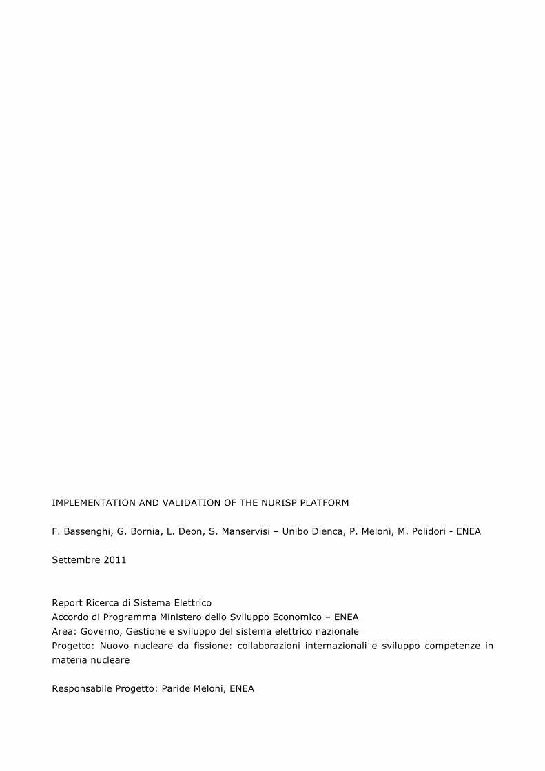
Figure 1.1: SALOME graphical user interface
SALOME is a free and open-source software released under the GNU LesserGeneral Public License. The source code and executables in binary form may bedownloaded from its official website at http://www.salome-platform.org. Thereare several version available, such as Debian, Mandriva and a universal package
13

NURISP platform implementation
with all dependencies inside. On the CRESCO-ENEA GRID the Mandriva version(for 64 bits) is installed. SALOME provides a generic platform for numericalsimulations and basic software for integration of custom modules and developing ofthe custom CAD applications. The main modules available are: KERNEL, GUI,GEOM, MESH, MED, POST and YACS. The KERNEL module is the generalservice manager. This module is the main module needed to perform the servicesand all the transfer files among the platform computers. SALOME can be usedgraphically by using the GUI module which enables the graphical user interface.The GEOM module can be used for CAD editing and import/export geometry.A mesh geometry may be constructed with this module that has all the CADfunctions. Over the resulting geometry the mesh can be generated by using theMESH module. The MESH module is constructed for standard meshing and forsupport of some external mesh generators. The MED module is the MED data filesmanagement. All the input and output files are written in MED formats and thismodule is used in all external reading and writing. The dedicated post-processorto analyze the results of solver computations is the POST module. We do not usethis module since the PARAVIEW program will be preferred. Finally the YACSmodule is the computational schema manager for multi-solver coupling and thesupervision module which can be used for weak code coupling.
SALOME is mainly used as mesh generator but it has potential for inter-operability between computational software, integration of new components intoheterogeneous systems and multi-physics weak coupling. The platform may inte-grate different additional codes on which perform code coupling. At the momentthe integration among codes of the NURISP platform is far to be completed butsome basic functionality can be used. In SALOME the ideas of weak and internalcoupling are implemented. In fact the weak coupling can be performed with theexchange of output and input files by using the YACS module. The idea of internalweak coupling, where all the equations are solved in a segregated way using shearedmemory to exchange data between codes, is implemented in the the MED libraryand its MEDMEM API classes. SATURNE has already a module that links to theSALOME platform in development at EDF. NEPTUNE and CATHARE codes arealso developing an integration module for the SALOME platform [31, 32].
The SALOME platform is located on CRESCO-ENEA GRID in the directory
/afs/enea.it/project/fissicu/soft/Salome
The salome platform can be run in two ways: from console and from FARO website.From console one must first set the access to the bin directory
/afs/enea.it/project/fissicu/soft/bin
by executing the script
14

NURISP platform implementation
$ source pathbin.sh
The script pathbin.shmust be in the home directory. One must copy the templatescript pathbin.sh from the directory
/afs/enea.it/project/fissicu/soft/bin
and then execute the script to add the bin directory to the PATH. If the pathbin.shscript is not available one must enter the bin directory to run the program.
Once the bin directory is on your own PATH all the programs of the platformcan be launched. The command needed to start the SALOME application is
$ salome
The script salome consists of two commands: the environment setting and thestart command. The environment script sets the environment of shell. The startcommand is a simple command that launches the runSalome command.
From FARO web applications the SALOME platform with remote acceleratedgraphics can be accessed. Once FARO has been started one must open an xterm.In the xterm console one must follow the same procedure as before. For detailson FARO see [2] and the main CRESCO-ENEA web page. First, set the access tothe bin directory
/afs/enea.it/project/fissicu/soft/bin
by executing the script
$ source pathbin.sh
SALOME starts with the command
$ salome
For details see [2].
1.2.2 NEPTUNE
15

NURISP platform implementation
NEPTUNE
Developer(s) EDFStable release June 7, 2010;Operating system Linux and Cross-platformLicense not free (use under NURISP written agreement)Website no website
CRESCO-ENEA GRID:
executable: neptuneinstall directory: /afs/enea.it/project/fissicu/soft/Neptune
Figure 1.2: Neptune graphical user interface.
The NEPTUNE project is a joint research and development program betweenEDF and CEA. The project provides a two-phase thermohydraulics CFD softwarefor studying nuclear reactor components. The code may perform three-dimensionalcomputations of the main components of the reactors: cores, steam generators,condensers, and heat exchangers. NEPTUNE supports from one to twenty fluidfields (or phases) and includes thermodynamic laws for water/steam flows. It isbased on advanced physical models, such as two-fluid equations combined with in-terface area transport and two-phase turbulence, and numerical methods such asunstructured finite volume solvers. The code is based on cell-centered type finitevolume method which can use meshes with all types of cell and nonconforming con-nections. NEPTUNE uses co-localized gradients with reconstruction methods to
16
NURISP platform implementation
compute face values and supports distributed-memory parallelism by domain split-ting. NEPTUNE is written in Fortran and organized in modules. The enveloppecomponent manages the pre-processing and the post-processing functions, whileedamox is the graphical user interface. One can introduce user functions by usingthe user Fortran module. The computational kernel is a FORTRAN programimplemented in the Neptune_CFD module [19, 20, 21, 22, 23].
The NEPTUNE code is located on CRESCO-ENEA GRID in the directory
/afs/enea.it/project/fissicu/soft/Neptune
The PATH for the home directory is
/afs/enea.it/project/fissicu/soft/bin
and can be set by executing the script
$ source pathbin.sh
as it is explained more in details in [2]. The NEPTUNE GUI on CRESCO-ENEAGRID starts with the command
$ neptune
Not all libraries are yet available at the moment for the CRESCO architecture.We suggest to run NEPTUNE GUI on a personal workstation. The GUI is usedto set up the simulation creating a param file. The solution of the case must berun in command line mode or in batch mode. For details see [2].
1.2.3 TRIO_U
TRIO_U
Developer(s) CEAStable release 1.61 / June, 2010;Operating system LinuxLicense not free (use only under written agreement)Website http://www-trio-u.cea.fr
CRESCO-ENEA GRID:
executable: triouinstall directory: /afs/enea.it/project/fissicu/soft/Triou
17
NURISP platform implementation
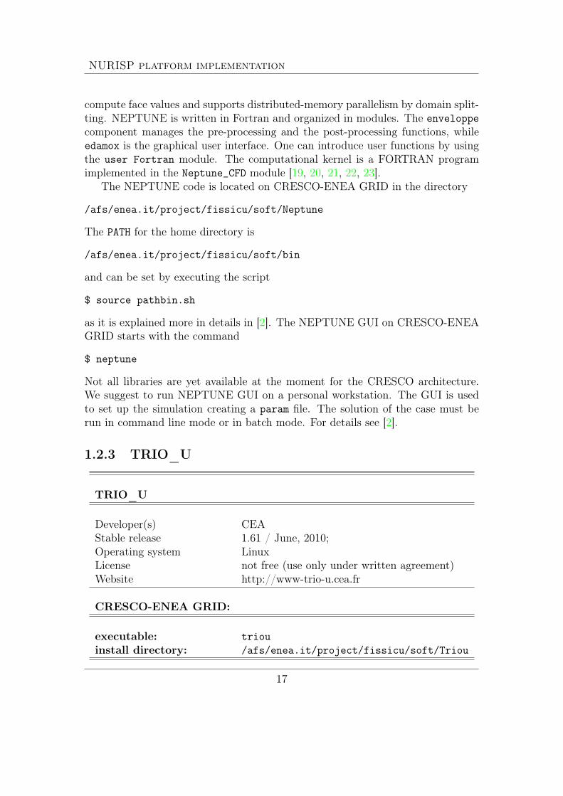
Figure 1.3: TRIO_U graphical user interface.
Trio_U is a project that aims to develop numerical simulation software forfluid dynamics. It is developed at the Laboratory of Modeling and Software De-velopment of the Directorate of Nuclear Energy of the CEA, This project startsas an object-oriented, parallel code dedicated to scientific and industrial applica-tions in the nuclear field. The variety of physical models and numerical methodsimplemented in this code allow to simulate various problems ranging from thelocal two-phase flow simulations to turbulent flows in industrial facilities or incomponents of nuclear reactors.
Inside the code two modules are available: a VDF module (finite differencevolume) and a VEF module (finite element volume not to be confused with thefinite element method). The VDF and VEF modules are designed to processthe 2D or 3D flow of Newtonian, incompressible or slightly incompressible fluidswhere the density is a function of a local temperature and concentration values(Boussinesq approximation). Non-Newtonian fluid by using the Otswald law arepossible [34, 35, 36].
It is planned to interface Trio_U with other simulation software supportedor developed by the CEA. For example SALOME-NEPTUNE or NEPTUNE-CATHARE. In particular the SALOME platform may be used for different stagesof the Trio_U calculation: creation of CAD and mesh editing of the data set [33].
18

NURISP platform implementation
The coupling NEPTUNE-CATHARE has been used in many physical situationswhen one plans to study a system component in full three-dimensional geometry.The domain is divided into two parts: the component and the rest of the system.NEPTUNE code is solved in the three-dimensional domain of the component withboundary conditions determined by the mono-dimensional CATHARE code thesolves the rest of the domain.
The TRIO_U code is located on CRESCO-ENEA GRID in the directory
/afs/enea.it/project/fissicu/soft/Triou
The PATH for the home directory is
/afs/enea.it/project/fissicu/soft/bin
The path can be set by executing the script
$ source pathbin.sh
The TRIO_U GUI on CRESCO-ENEA GRID starts with the command
$ triou
The GUI, shown in Figure 1.3, is used to set up the simulation creating a paramfile. The solution of the case must be run in command line mode or in batch mode.For details see [2].
1.2.4 SATURNE
SATURNE
Developer(s) EDFStable release 2.0.0 RC2 / July 7, 2010;Operating system Linux and Cross-platformLicense GNU General Public LicenseWebsite http://www.code-saturne.org
CRESCO-ENEA GRID:
executable: saturneinstall directory: /afs/enea.it/project/fissicu/soft/Saturne
19

NURISP platform implementation
Figure 1.4: SATURNE graphical user interface.
SATURNE is a general purpose CFD free software. Developed since 1997 atEDF R&D, SATURNE is now distributed under the GNU GPL license. It isbased on a collocated Finite Volume approach that accepts meshes with any typeof cell. The code works with tetrahedral, hexahedral, prismatic, pyramidal andpolyhedral finite volumes and any type of grid structures such as unstructured,block structured, hybrid, conforming or with hanging node geometries.
Its basic capabilities enable the handling of either incompressible or compress-ible flows with or without heat transfer and turbulence. Many turbulence modelare implemented such as mixing length, κ-ε models, κ-ω models, v2f , Reynoldsstress models and Large Eddy Simulation (LES). Dedicated modules are avail-able for additional physics such as radiative heat transfer, combustion (gas, coaland heavy fuel oil), magneto-hydro dynamics, compressible flows, two-phase flows(Euler-Lagrange approach with two-way coupling), extensions to specific applica-tions (e.g. for atmospheric environment) [29, 30].
SATURNE can be coupled to the thermal software SYRTHES for conjugateheat transfer. It can also be used jointly with the structural analysis softwareCODE_ASTER, in particular in the SALOME platform. Both SYRTHES andCODE_ASTER are developed by EDF and distributed under the GNU GPLlicense.
The SATURNE code is located on CRESCO-ENEA GRID in the directory
/afs/enea.it/project/fissicu/soft/Saturne
The PATH for the home directory is
20

NURISP platform implementation
/afs/enea.it/project/fissicu/soft/bin
This PATH can be set by executing the script
$ source pathbin.sh
The SATURNE GUI on CRESCO-ENEA GRID starts with the command
$ saturne
The GUI, shown in Figure 1.4, is used to set up the simulation creating a paramfile. The solution of the case must be run in command line mode or in batch mode.For details see [2].
1.2.5 CATHARE
CATHARE
Developer(s) CEAStable release Cathare 2 v2_5;Operating system Linux and Cross-platformLicense licence agreement from CATHAREWebsite http://www-cathare.cea.f
CRESCO-ENEA GRID:
executable: cathareinstall directory: /afs/enea.it/project/fissicu/soft/cathare
CATHARE or Code for Analysis of thermohydraulics during an Accident ofReactor and safety Evaluation (CATHARE) is a system code for PWR safetyanalysis, accident management, definition of plant operating procedures and forresearch and development. It is also used to quantify conservative analysis marginsand for licensing.
The CATHARE code is located on CRESCO-ENEA GRID in the directory
/afs/enea.it/project/fissicu/soft/Cathare
The PATH for the home directory is
/afs/enea.it/project/fissicu/soft/bin
21

NURISP platform implementation
Figure 1.5: CATHARE graphical user interface (GUITHARE).
The CATHARE GUI (GHITHARE) on CRESCO-ENEA GRID starts with the com-mand
$ cathare
The GUI, shown in Figure 1.5, is used to set up the simulation creating a paramfile. The solution of the case must be run in command line mode or in batch mode.For details see [2].
1.3 Platform pre- and post-processing operationsThe way in which a code writes and reads input and output data is a very importantand sensitive issue. Each software supports a limited number of input and outputformats that are often not supported by other codes. An important aim of anyplatform is to uniform all the reading/writing formats so that all the codes canuse the same format for input and output files. Concerning the input formatwe consider mainly the MED and XDMF formats. Both MED and XDMF aredriver files that access the information stored by files in HDF5 format. The HDF5library is capable of storing large amounts of data in a hierarchically structured
22

NURISP platform implementation
form. Regarding the output viewer we choose PARAVIEW because it is opensource and can manage a large number of formats.
1.3.1 Input/output formats
Figure 1.6: HDF data viewer
One of the most interesting input/output formats is the HDF5 format. Hi-erarchical Data Format, commonly abbreviated HDF5, is the name of a set offile formats and libraries designed to store and organize large amounts of numer-ical data [16]. The HDF format is available under a BSD license for general useand is supported by many commercial and non-commercial software platforms,including Java, Matlab, IDL, and Python. The freely available HDF distribu-tion consists of the library, command-line utilities, test source, Java interface,and the Java-based HDF Viewer (HDFView). Further details are available athttp://www.hdfgroup.org. This format supports a variety of datatypes, and isdesigned to give flexibility and efficiency to the input/output operations in the caseof large amounts of data. HDF5 is portable from one operating system to anotherand allows forward compatibility. In fact old versions of HDF5 are compatiblewith newer versions.
The great advantage of the HDF format is that it is self-describing, allowing anapplication to interpret the structure and contents of a file without any externalinformation. There are structures designed to hold vector and matrix data. OneHDF file can hold a mixture of related structures which can be accessed as a groupor as individual objects. The HDF5 has a very general model which is designedto conceptually cover many specific data models. Many different kinds of datacan be mapped to HDF5 objects, and therefore stored and retrieved using HDF5.
23

NURISP platform implementation
The HDF5 project provides also a visualization tool, HDFVIEW (shown in Figure1.6), to access raw HDF5 data. This program can be run from terminal by simplytyping
$ hdfview
Figure 1.7: XDMF data view
XDMF (eXtensible Data Model and Format) is a library providing a standardway to access data produced by HPC codes. The information is subdivided intoLight data, that are embedded directly in the XDMF text file, and Heavy datathat are stored in an external file. Light data are stored using XML, Heavy dataare typically stored using HDF5. A Python interface exists for manipulating bothLight and Heavy data. ParaView, VisIt and EnSight visualization tools are ableto read XDMF [39].
The organization of XDMF begins with the Xdmf element. Any element canhave a Name or a Reference attribute. A Domain can have one or more Gridelements. Each Grid must contain a Topology, a Geometry, and zero or more
24

NURISP platform implementation
Attribute elements. Topology specifies the connectivity of the grid while Geometryspecifies the location of the grid nodes. Attribute elements are used to specifyvalues such as scalars and vectors that are located at the node, edge, face, cellcenter, or grid center. As an example, the following file displays the Figure 1.7
<?xml version="1.0" ?><!DOCTYPE Xdmf SYSTEM "Xdmf.dtd" []><Xdmf> <Domain> <Grid Name="TestGrid">
<Topology Type="Hexahedron" NumberOfElements="2" ><DataItem Format="XML" DataType="Float" Dimensions="2 8">
0 1 7 6 3 4 10 9 1 2 8 7 4 5 11 10</DataItem>
</Topology><Geometry Type="XYZ"><DataItem Format="XML" DataType="Float" Precision="8"Dimensions="4 3 3">
0.0 0.0 1.0 1.0 0.0 1.0 3.0 0.0 2.00.0 1.0 1.0 1.0 1.0 1.0 3.0 2.0 2.00.0 0.0 -1.0 1.0 0.0 -1.0 3.0 0.0 -2.00.0 1.0 -1.0 1.0 1.0 -1.0 3.0 2.0 -2.0
</DataItem></Geometry><Attribute Name="NodeValues" Center="Node"><DataItem Format="XML" DataType="Float" Precision="8"Dimensions="4 3" >
100 200 300300 400 500300 400 500500 600 700
</DataItem></Attribute><Attribute Name="CellValues" Center="Cell">
<DataItem Format="XML" DataType="Float" Precision="8"Dimensions="2" >
100 200</DataItem>
</Attribute></Grid> </Domain> </Xdmf>
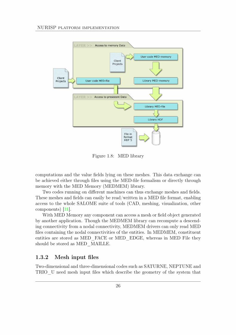
The MED (Modèle d’Echange de Données) data exchange model is the formatused in the SALOME platform for communicating data between different com-ponents. It manipulates objects that describe the meshes underlying scientific
25
NURISP platform implementation
Figure 1.8: MED library
computations and the value fields lying on these meshes. This data exchange canbe achieved either through files using the MED-file formalism or directly throughmemory with the MED Memory (MEDMEM) library.
Two codes running on different machines can thus exchange meshes and fields.These meshes and fields can easily be read/written in a MED file format, enablingaccess to the whole SALOME suite of tools (CAD, meshing, visualization, othercomponents) [31].
With MED Memory any component can access a mesh or field object generatedby another application. Though the MEDMEM library can recompute a descend-ing connectivity from a nodal connectivity, MEDMEM drivers can only read MEDfiles containing the nodal connectivities of the entities. In MEDMEM, constituententities are stored as MED_FACE or MED_EDGE, whereas in MED File theyshould be stored as MED_MAILLE.
1.3.2 Mesh input files
Two-dimensional and three-dimensional codes such as SATURNE, NEPTUNE andTRIO_U need mesh input files which describe the geometry of the system that
26
NURISP platform implementation
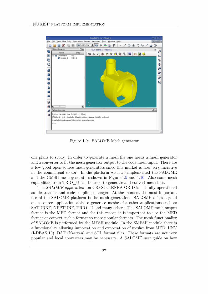
Figure 1.9: SALOME Mesh generator
one plans to study. In order to generate a mesh file one needs a mesh generatorand a converter to fit the mesh generator output to the code mesh input. There area few good open-source mesh generators since this market is now very lucrativein the commercial sector. In the platform we have implemented the SALOMEand the GMSH mesh generators shown in Figure 1.9 and 1.10. Also some meshcapabilities from TRIO_U can be used to generate and convert mesh files.
The SALOME application on CRESCO-ENEA GRID is not fully operationalas file transfer and code coupling manager. At the moment the most importantuse of the SALOME platform is the mesh generation. SALOME offers a goodopen source application able to generate meshes for other applications such asSATURNE, NEPTUNE, TRIO_U and many others. The SALOME mesh outputformat is the MED format and for this reason it is important to use the MEDformat or convert such a format to more popular formats. The mesh functionalityof SALOME is performed by the MESH module. In the SMESH module there isa functionality allowing importation and exportation of meshes from MED, UNV(I-DEAS 10), DAT (Nastran) and STL format files. These formats are not verypopular and local converters may be necessary. A SALOME user guide on how
27

NURISP platform implementation
to generate a simple mesh can be found in [2]. More substantial help for meshcreation can be found at
http://www.salome-platform.org/user-section/salome-tutorials
where ten exercises from EDF in mesh generation can be found.Another mesh generator in the platform is the GMSH application implemented
under the TRIO_U directory. GMSH is a freeware to build 2D/3D unstructuredmeshes with tetrahedral or hexahedral meshes. Meshes generated by GMSH mustbe translated to Trio_U format by a converter located in $TRIO_U_ROOT/GMSHdirectory. It can also be run from the GUI of Trio_U using the button GMSH.
Figure 1.10: GMSH mesh generator
The TRIO_U application implemented in the platform has some mesh andconverter capabilities. Mesh converters from Fluent to MED and UNV formatscan be found inside this code. Details are available in the TRIO_U documentation.A mesh file may be created for Trio_U by using one of the following software:a) Xprepro mesh generator for Cartesian 2D/3D domain;b) GMSH freeware mesh generator for VEF 2D/3D domain;c) Trio_U mesh generator for simple geometries;d) ICEM, IDEAS, SIMAIL mesh generator for VEF 3D domains;e) translator for mesh format from Gambit to Trio_U.Xprepro is a new tool for Trio_U code that can create very complex 2D, 3D VDFmeshes. You can run Xprepro either from a study opened with the GUI of Trio_Uthrough a button named Mesh, or by running the command line Xprepro.
28

NURISP platform implementation
An instruction in the TRIO_U data set is available to reread meshing issuedby Gambit/Tgrid (tools from Fluent) using Trio_U. This instruction is as follows:
Lire_Tgrid dom nom_fichier_maillage
where dom corresponds to the domain name, nom_fichier_maillage correspondsto the file containing the mesh. 2D (triangles or quadrangles) and 3D (tetra or hexaelements) meshes may be read by Trio_U. The template for the Gambit/MEDconverter can be found in the directory
/afs/enea.it/project/fissicu/soft/triou/data
The file is as following
dimension 3Domaine domLire_tgrid dom mesh.mshecrire_med dom mesh.medFin
An instruction in the TRIO_U data set is available to read MED mesh issued forexample from SALOME. This instruction is as follows
Lire_Med [vef][fam_name_from_gr_name] mesh_name filename.med dom_name
The dom_name corresponds to the domain name, filename.med is the file (writtenin MED format) containing the mesh named mesh_name. Option vef is obsoleteand is kept for backward compatibility. The option fam_names_from_gr_nameuses the group names instead of the family names to detect the boundaries into aMED mesh.
1.3.3 The PARAVIEW application
Various applications are available inside the platform for visualization. The twomain visualization applications implemented on the FISSICU platform are VISITand PARAVIEW. In order to uniform the output and the visualization we useonly the PARAVIEW software and therefore the output files must be saved in aPARAVIEW readable format. Sometimes the use of VISIT could be convenientwith the TRIO_U application since VISIT can read its own natural format. Theuse of PARAVIEW does not impose substantial limitations since PARAVIEWreads a large number of formats. It is an open-source, multi-platform applicationdesigned to visualize large size data sets. PARAVIEW uses the VisualizationToolkit (VTK) as the data processing and rendering engine and has a user interfacewritten using the Qt libraries [38]. The Visualization Toolkit (VTK) provides
29

NURISP platform implementation
Figure 1.11: Basic interface for PARAVIEW
the basic visualization and rendering algorithms. VTK incorporates several otherlibraries to provide basic functions such as rendering, parallel processing, parallelrendering. It is built on an modular structure and runs on distributed and sharedmemory parallel as well as single processor systems.
A brief explanation of the PARAVIEW GUI is given in Figure 1.11. The GUIhas many panels that control the visualization. The two main panels are the ViewArea and the Pipeline Browser panel. The data are loaded in the View Area whichdisplays visual representations of the data in 3D View, XY Plot View, Bar ChartView or Spreadsheet View. The visualization on the View Area is managed by thePipeline Browser panel. The Open and Save data buttons perform the loadingand saving operations for all the supported file formats. The Object Inspectorpanel contains controls and information about the reader, source, or filter selectedin the Pipeline Browser. The most important menu is the Filters menu that isused to manipulate the data. For example one can draw the isolines of any datasetusing the Contour filter. The Sources menu is used to create new geometricalobjects while the Animation toolbar navigates through the different time steps of
30

NURISP platform implementation
the simulation [27].In ENEA-CRESCO grid, the PARAVIEW application can be run in two differentmodes:a) X11 console mode;b) remote application mode through FARO application.
From X11 console the command
$ paraview-3.10.0
runs the latest version of PARAVIEW (3.10.0). The other versions are availableby typing the version number in the command after the − sign. PARAVIEW canbe launched only from machines with graphical capability. The machines withgraphical capability have a letter g in the name. For example PARAVIEW canrun from cresco1-fg1.portici.enea.it.
As a remote application one must login from the FARO web page and thenselect the PARAVIEW button. If the program runs in this mode the renderingis pre-processed on the remote machine, which guarantees higher speed imageprocessing (see [2]).
1.4 Platform code coupling and servicesThe platform SALOME has many capabilities. Among them there are the SA-LOME clustering system service, the SALOME module service and YACS codecoupling service. The clustering service system allows file transfers inside the gridand therefore from one computer to another. The SALOME module service canintegrate a new code as a SALOME module transferring all the SALOME graph-ical capabilities to this module. Reading and writing parameter data can be doneusing the SALOME graphical built-in functions. The application YACS allowsdifferent codes to run in sequence and transform output data of an applicationinto input data for another application.
1.4.1 SALOME clustering service system
In a SALOME application, distributed components, servers and clients use theCORBA middleware for communication. The main services of the clustering sys-tem are: component services, file transfer services and batch services. The com-ponent services define the container such a machine, an operative system, etc.This component can then be identified and used for various operations. The filetransfer services transfer files between one computer and another. This is funda-mental for many input/output and graphical operations. The batch services run
31

NURISP platform implementation
programs in batch mode. For some general purpose services, the CORBA interfaceis encapsulated in order to provide a simple interface. Encapsulation is generallydone in C++ classes. All the different CORBA interfaces are available for usersin Python. A Python SWIG interface is also generated from C++, to ensure aconsistent behavior between C++ modules and Python modules or user scripts.SALOME_FileTransferCORBA is responsible for file transfer. There is a class for fileservice written in C++ and a corresponding file transfer service in Python. Pythoninterface is obtained by using the SWIG library from C++. The following exampleshows how to transfer a file from a remote host to the client computer. Remotehostname is computer0 and we would like to copy path/file.tar.gz from remoteto local computer. A full pathname is required. A container is created on remotecomputer if it does not exist, to handle the file transfer.
# Salome set up --------------import salomesalome.salome_init()# LifeCycleCORBA set up -------import LifeCycleCORBA# remote file name -------remotefile="path/file.tar.gz"# transfer -------aFileTransfer=LifeCycleCORBA.
SALOME_FileTransferCORBA(’computer0’,remotefile)localFile=aFileTransfer.getLocalFile()
Another way to have a service access is through the SALOME batch service. Theinterested reader can consult the SALOME documentation.
1.4.2 SALOME module and code integration
In order to integrate a code inside the Salome platform one can run the code as aSALOME module. For this reason one must develop a simple SALOME modulewhich contains the application code. This module and the associated program canthen be loaded in the SALOME GUI in order to have a graphical interface anduse all the graphical resources available inside the SALOME platform.
The steps in the module development are as follows:1) create a module tree structure;2) create a SALOME component that can be loaded by a C++ or Python SA-LOME container, then configure the module so that the component is known toSALOME; 3) add a graphic GUI.
The first step in the development process is the creation of the module treefile structure. The typical SALOME module usually includes some set of the
32

NURISP platform implementation
configuration files (used in the build procedure of a module), Makefiles, IDL filethat provides a definition of CORBA services implemented in a module and a set ofsource Python files which implement the module CORBA engine and (optionally)its GUI.
The module command will not work until the following environment variableshave been set
export KERNEL_ROOT_DIR=<KERNEL installation="" path>="">export MYMODULE_ROOT_DIR=<MYMODULE installation="" path>="">
In order to activate a module in the SALOME GUI desktop, the user shouldpress the module button on the Modules toolbar or select the name of the modulein the combo box on this toolbar. The image file to be used as an icon of a moduleshould be exported by the module build procedure. The icon file name is definedin the corresponding SalomeApp.xml configuration file
<section name="MYMODULE"><parameter name="name" value="MYMODULE"/><parameter name="icon" value="MYMODULE.png"/><parameter name="library" value="SalomePyQtGUI"/>
</section>
In order to run the module one must go to the
MYMODULE\_module\_installation\_dir
directory and type
./bin/salome/runAppli
This command runs SALOME session configured for KERNEL and the module.
1.4.3 Coupling codes inside SALOME platform
The SALOME platform contains the YACS module that is an application thatallows calculation schemes. These calculation schemes can be generalized to in-put/output file exchange to provide a first approach to weak coupling betweenapplications.
The basic element of a calculation scheme is the calculation node. A calcula-tion node is an elementary action ranging from a simple multiplication to a localexecution of a script or a remote execution of a SALOME component service. Thecalculation scheme is a complex set of calculation nodes which are connected byinput and output ports. Through these ports, data may be exchanged between
33

NURISP platform implementation
nodes. Loops, switch- and if-statements are used to modularize a calculationscheme and define iterative processes.
If one considers a port as a datastream port then it can be used to exchange dataduring execution. At the moment this type of port is only supported by nodesrelated to SALOME components. A datastream port has a name, a direction,which goes from input to output, and a type. This type is the type of a CORBAobject that manages the data exchange. It is not a simple task to implementa datastream port and therefore SALOME provides a ready made port calledCALCIUM datastream port. This port is designed to ease scientific code coupling.
The CALCIUM library enables fast and easy coupling of Fortran/C/C++ codesin a simple and not very intrusive manner. By using these functions one can controlthe number of simultaneous executions of the different codes and transmission linksbetween connection points. Connection points, which are typed by simple types,can operate on the time or iterative mode. Data are produced and read in codesby a call. When non-existing data are requested the reader can obtain interpolateddata in time mode. The program is paused if the reader is waiting for data thatwill never be produced. In this case the application proposes either the stop of theexecution or the extrapolation of the requested data.
34
Chapter 2
Validation of the CATHARE modelof the SPES-99 facility
2.1 THE SPES-99 FACILITY
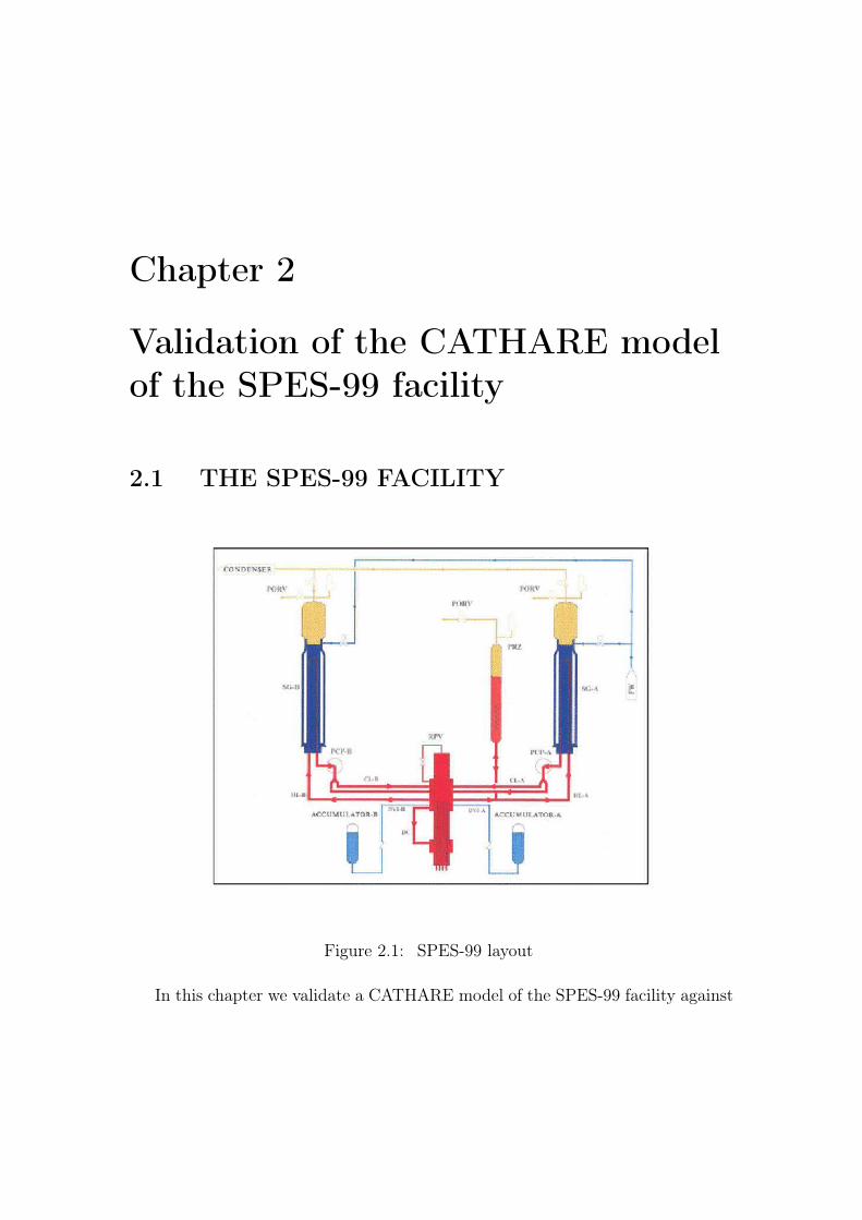
Figure 2.1: SPES-99 layout
In this chapter we validate a CATHARE model of the SPES-99 facility against

Validation of the CATHARE model of the SPES-99 facility
an Intermediate Break LOCA experimental test. The SPES-99 circuit is a fullpressure, full height, two-loop experimental test facility simulating a commercialsize PWR, with an overall scaling factor of about 1 : 400. It basically consists ofa primary and a secondary circuit up to the steam isolation valves together withaccumulators. The steam isolation valves and the accumulators are part of thesafety system to protect the plant in case of accident. The SPES facility, locatedat SIET laboratories in Piacenza (Italy), was modified after five years of inactivityfrom the SPES-2 configuration [28] to SPES-99 [14], in view of possible futureprograms leading to investigate intermediate break transient phenomena, whichhad never been simulated before in the facility. The current scheme of the SPES-99 facility is shown in Figure 2.1. Each of the two primary loops includes a HotLeg (HL) and two Cold Legs (CL). The hot leg connects the reactor pressure vesselto the steam generator. The two cold legs detach from a single primary coolantpump vertical discharge line. A device simulating a 10 inch equivalent break ismounted on the cold leg 2 of loop B to carry out the intermediate break test.
Cooling Fluid waterNumber of loops 2Number of pumps 2
Design Primary Pressure [MPa] 20Design Secondary Pressure [MPa] 20Primary Design Temperature [C] 365Design Secondary Temperature [C] 310
Maximum Power [MW] 9Height Scaling factor 1:1
Table 2.1: Main Characteristics of SPES-99
The reactor pressure vessel is composed of the lower plenum, the riser, wherethe rod bundle is placed, the upper head and the down-comer. The down-comerconsists of an annular section, where the four cold legs and the two Direct VesselInjection (DVI) nozzles are attached, and an outer pipe connecting the annularsection to the lower plenum. The rod bundle is electrically heated and consistsof 97 skin heated Inconel rods with a maximum power of 7MW . The pressurizerconsists of a cylindrical flanged vessel equipped with two immersed heaters and sixexternal ones. It is connected to the hot leg of the intact loop A. The pumps arecentrifugal, single stage, horizontal shaft type. The suction line is horizontal andthe delivery is vertical, discharging downwards into a pipe upstream of the twocold legs. The facility has two identical steam generators (SG) to transfer thermalpower from the primary to the secondary circuit. The SG primary side consists ofa 13 Inconel600 tube bundle, assembled in a square lattice, and inlet/outlet plena.
36

Validation of the CATHARE model of the SPES-99 facility
The secondary side has full elevation up to the top of the steam separator and thesecondary separators (dryers) are located at the SG top. The main characteristicsof the SPES 99 facility are reported in Table 2.1.
2.2 CATHARE 2 Code and SPES-99 Model
Figure 2.2: Vessel nodalization
CATHARE (Code for Analysis of THermalhydraulics during an Accident ofReactor and safety Evaluation) is a system code developed for the transient andaccident analysis in PWRs. It was used to support the licensing process of Frenchpower plants (N4, EPR) [37, 26]. The present CATHARE2 code, started in 1979,is the result of a collaboration among CEA (Commissariat à l’Energie Atomique),IRSN (Institut de Radioprotection et de Sureté Nucléaire), EDF (Electricité deFrance) and AREVA NP. CATHARE [8, 4] treats the thermal-hydraulics of theheat-transfer fluid by means of a non-homogeneous and non-equilibrium two-fluidmodel (liquid and vapor) based on 4 scalar equations (mass and energy), 2 vectorequations (momentum), for the 6 main parameters: liquid and gas enthalpy (Hl,Hg), liquid and gas velocity (Vl, Vg), pressure (P) and void fraction (α). It includesthe transport equations to take into account up to 4 non-condensable gases and 12radio-chemical components. A fully implicit solution scheme is adopted for 0-D and
37

Validation of the CATHARE model of the SPES-99 facility
Figure 2.3: Loop A nodalization
1-D modules and a semi-implicit scheme for 3-D module. The modular structureof the code allows the parallel computation. The code relies on a unique set ofqualified physical correlations and generic component models (1-D, 0-D and 3-Dand Boundary Conditions modules) for the closure relationship to calculate mass,momentum and energy exchange between the two phases and between each phaseand the boundaries of the thermal-hydraulic system. Sub-modules for specialcomponents and processes are also available: source, sink, valve, pump, break,SG, etc. In addition, special process models are foreseen for active walls, fuel etc.The high degree of maturity achieved by the CATHARE 2 code makes it a toolable to simulate practically every kind of LWR with high confidence, includingconventional thermal-hydraulic loops like the integral test facility.
The latest version V2.5_1 of CATHARE 2 is adopted to simulate the SPES-99
38

Validation of the CATHARE model of the SPES-99 facility
facility; the related nodalization is compliant with the geometrical dimensions ofthe different parts and components as well as the topology of the circuits [40].In particular, the modular structure of the code allows to find a good balanceto preserve heights, flow areas and fluid volumes. It is worth reminding that thefacility is scaled 1 : 1 in height and 1 : 397 in volume with respect to the AP-600reactor. In Figures 2.2 and 2.3 the nodalization schemes of the primary vessel andof the loop A that includes the pressurizer are reported.
Some choices on the nodalization of the facility can strongly influence the re-sults of the simulation. The vessel annular downcomer is represented with a 0-Dcomponent (DWC_ANN) in order to easy describe the high number of connectionsin this part of the circuit (4 cold legs, downcomer-upper head bypass, accumula-tors injection, tubular downcomer). On the other hand this component does notallow to take into account the inertial forces (the internal velocity is neglected)and the possible multi-D effects. The employment of axial or 3D components isnot considered in the present work but will be evaluated with future sensitivityanalysis. The accumulators are simulated by the specific CATHARE sub-modulesthat do not allow a detailed description of the discharge line. The thermal capacityof the wall structure could have effect on the gas expansion and therefore on thewater injection behavior.
2.3 SPES-99 facility steady state
Steady State Conditions Experimental Values CATHARE ValuesHeater Rod Power (MW) 4.97 4.92
Pressurized Pressure (MPa) 15.37 15.36Core Inlet Temp. [oC] 277.9 273.4Core Outlet Temp. [oC] 320.4 312.7
Core Mass Flowrate [kg/s] 23.55 23.55DC-UH bypass Mflow [kg/s] 0.13 0.13
Pressurizer level [m] 3.77 3.72
Table 2.2: Steady state main parameters (1)
2.3.1 Steady state
The CATHARE code has an algorithm (PERMINIT) that provides the initialsteady state conditions of the thermal-hydraulic parameters starting from a set ofguess values and introduces the necessary corrections to achieve the convergence.
39

Validation of the CATHARE model of the SPES-99 facility
Steady State Conditions Exp Val CATH Val Exp Val CATH ValCL Temp. (A1, B1) [oC] 279.7 277.6 273.8 272.9CL Temp. (A2, B2) [oC] 279.4 277.6 273.8 272.9HL Temp. (A, B) [oC] 315.8 316.9 312.5 312.5
CL MFlow (A1,B1) [kg/s] 6.04 5.56 6.23 5.78CL MFlow (A2,B2) [kg/s] 6.24 5.82 6.05 5.65Pump speed (A, B) [rpm] 3057 2769 2453 2299SG pressure (A , B) [MPa] 4.97 4.94 4.96 4.96SG Dome level (A , B) [m] 0.8 0.8 0.8 0.8SG FW Temp. (A ,B) [oC] 225.6 226.9 226.0 226.0
SG Dome Pres. (A ,B) [MPa] 5.16 5.08 4.97 4.97SG FW flowrate (A ,B) [kg/s] 2.00 2.20 1.41 1.32
Table 2.3: Steady state main parameters (2)
This is the first step to obtain the reference steady state that was recorded on thefacility before running the Intermediate Break LOCA test. In order to get thermal-hydraulic conditions closer to the reference steady state a calibration procedureof the main parameters is adopted. This objective is achieved according to aprocedure recommended for CATHARE [9] by running the transient computationalgorithm (TRANSIENT) and controlling the main parameters directly in theinput-deck. To this purpose, we act on the boundary through a proportional-integral adjustment. The following parameters: primary mass flowrate, liquidlevel in the pressurizer, primary pressure, fluid inventory in the steam generatorsand feed-water mass flowrate are controlled for 3500 seconds until the acceptancecriteria are satisfied. After stopping all the adjustments, we run the code for other1500 seconds to verify the stability of the achieved steady state. The results arecompared with the experimental values in Tables 2.2-2.3.
Important deviations are related to the temperatures in the primary circuit thatare about 4 oC lower than the measured values, and the pump rotation velocitiesthat result 20% lower than the experimental ones.
2.3.2 Reference steady state
The adjustment towards the experimental data allows us to reduce the uncertain-ties related to certain phenomenologies and to obtain a reference steady state ingood agreement with the experimental results. The lower values of the primarytemperatures calculated by CATHARE indicate an over-prediction of the SG heattransfer that is justified by the uncertainties on the heat transfer coefficients andon the fouling degree of the SG tubes. In order to compensate this difference the
40
Validation of the CATHARE model of the SPES-99 facility
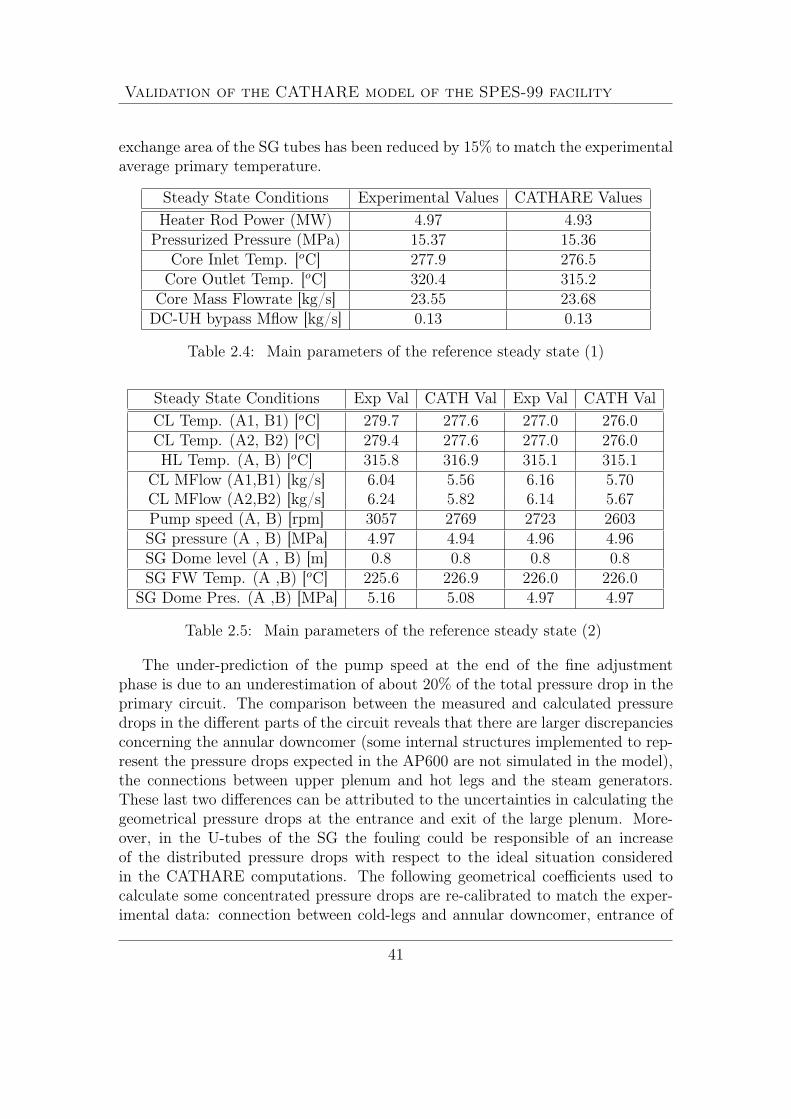
exchange area of the SG tubes has been reduced by 15% to match the experimentalaverage primary temperature.
Steady State Conditions Experimental Values CATHARE ValuesHeater Rod Power (MW) 4.97 4.93
Pressurized Pressure (MPa) 15.37 15.36Core Inlet Temp. [oC] 277.9 276.5Core Outlet Temp. [oC] 320.4 315.2
Core Mass Flowrate [kg/s] 23.55 23.68DC-UH bypass Mflow [kg/s] 0.13 0.13
Table 2.4: Main parameters of the reference steady state (1)
Steady State Conditions Exp Val CATH Val Exp Val CATH ValCL Temp. (A1, B1) [oC] 279.7 277.6 277.0 276.0CL Temp. (A2, B2) [oC] 279.4 277.6 277.0 276.0HL Temp. (A, B) [oC] 315.8 316.9 315.1 315.1
CL MFlow (A1,B1) [kg/s] 6.04 5.56 6.16 5.70CL MFlow (A2,B2) [kg/s] 6.24 5.82 6.14 5.67Pump speed (A, B) [rpm] 3057 2769 2723 2603SG pressure (A , B) [MPa] 4.97 4.94 4.96 4.96SG Dome level (A , B) [m] 0.8 0.8 0.8 0.8SG FW Temp. (A ,B) [oC] 225.6 226.9 226.0 226.0
SG Dome Pres. (A ,B) [MPa] 5.16 5.08 4.97 4.97
Table 2.5: Main parameters of the reference steady state (2)
The under-prediction of the pump speed at the end of the fine adjustmentphase is due to an underestimation of about 20% of the total pressure drop in theprimary circuit. The comparison between the measured and calculated pressuredrops in the different parts of the circuit reveals that there are larger discrepanciesconcerning the annular downcomer (some internal structures implemented to rep-resent the pressure drops expected in the AP600 are not simulated in the model),the connections between upper plenum and hot legs and the steam generators.These last two differences can be attributed to the uncertainties in calculating thegeometrical pressure drops at the entrance and exit of the large plenum. More-over, in the U-tubes of the SG the fouling could be responsible of an increaseof the distributed pressure drops with respect to the ideal situation consideredin the CATHARE computations. The following geometrical coefficients used tocalculate some concentrated pressure drops are re-calibrated to match the exper-imental data: connection between cold-legs and annular downcomer, entrance of
41

Validation of the CATHARE model of the SPES-99 facility
Table 2.6: Test boundary conditions
42

Validation of the CATHARE model of the SPES-99 facility
hot legs from the upper plenum, connections between hot/cold-legs and SG plena.The final results of the reference steady state computation are reported in Tables2.4-2.5.
It can be noticed that all the thermal-hydraulic parameters computed byCATHARE are in good agreement with the experimental data except for the feed-water mass flowrate in both secondary loops. In fact for this parameter CATHAREprovides a value of 1, 4 kg/s against the value of 2 kg/s as indicated on the ex-perimental report. A thermal balance carried out on both secondary loops shows
Figure 2.4: PRZ, SG-A, SG-B pressure and core power
that the calculated value is realistic whereas the experimental data is affected bya relevant error whose reason is not clear from the information indicated on theexperimental report.
2.4 SPES-99 IB LOCA transient
2.4.1 Results of the experiment
The Intermediate Break LOCA test consists of a 10 inch equivalent break in ColdLeg B2 starting from full power and full pressure conditions. The test was defined
43

Validation of the CATHARE model of the SPES-99 facility
Figure 2.5: ACC-A/B flow rate and heater rod temperature
by a working group of ENEA, ANPA, JRC Ispra, ANSALDO, Pisa University andSIET [11]. The experimental boundary conditions of the test are reported in Table2.6 together with the relevant thermal-hydraulic events.
The main phases of the transient can be summarized in the following steps:- a fast depressurization after the break;- the first heater rod heat-up due to DNB;- the intervention of the accumulator with quench of the first heat-up;- the continuous loss of mass from the break and the second heat-up due to dry-outof the core;- the end of the test for electric power supply interruption at the cladding temper-ature of 664 oC .
The trends of the main quantities with the indication of the events are shownin Figure 2.4 and Figure 2.5.
44

Validation of the CATHARE model of the SPES-99 facility
Table 2.7: Power curve
2.4.2 Comparison between post-test results and experimen-tal data
The IB LOCA test is computed with the CATHARE model described in the pre-vious paragraph. The transient computation starts from the reference steady stateconditions achieved after the fine adjustment phase (Tables 2.4-2.5). The bound-ary conditions reported in Table 2.6 as well as the power curve provided in theexperiment and described in Table 2.7 are imposed by the transient algorithm ofCATHARE. The main calculated parameters are compared with the experimentaltrends in Figures 2.6-2.10.
The Figure 2.6 shows the fast depressurization of the primary system. After theinitial period of the transient where this behavior is well predicted by CATHARE,
Figure 2.6: Pressurizer pressure
45

Validation of the CATHARE model of the SPES-99 facility
Figure 2.7: Accumulator A injection mass flow rate
the computed depressurization is a bit quicker than in the experiment. The slightlyearlier intervention of the accumulators highlighted in Figures 2.7-2.8 is a directconsequence of the quicker depressurization of the loop, whereas the prediction ofthe injection behavior without interruption is due to the lack of the short periodof re-pressurization in the CATHARE computation. Both discrepancies could berelated to the low resolution used in the geometrical description of the downcomerand accumulator injection line.
In order to improve the simulation of the quick depressurization phase of thetransient a more detailed model than the present 0-D volume should be adoptedfor the downcomer. We must take into account the inertial forces and the multi-Deffects of the 3-D components together with a more realistic description of thethermal capacity of the internal structures.
Figure 2.8: Integral mass injected by the accumulators
46

Validation of the CATHARE model of the SPES-99 facility
Figure 2.9: Rod Clad Temperature in Lower Power Channel (left) andLower/Middle Power Channel (right)
In spite of these discrepancies the occurrence of DNB phenomena is well pre-dicted by the code. In particular, at the lower/middle level (Figure 2.9 on the right)the rod heat-up time is precisely computed. The first peak in the clad temperatureis higher than that in the experiment and the effect of the mesh refinement in thepower channel should be investigated. The Figures 2.7-2.10, that report the rodclad temperature at four different levels, show that the intervention of the accu-mulator is effective in quenching the first heat-up of the heated rods. The secondpart of the transient, showing the mass loss from the break until the core dry-out,is computed in good agreement with the experiment. The occurrence of the secondheat-up at about 2000 s is well predicted by the code at the different levels of thepower channel, but with a slight delay compared to experimental data. Again, themesh refining in the power channel could be beneficial in improving the results ofthe simulation. The correct computation of the dry-out occurrence may denotea correct evaluation of the primary fluid inventory and therefore of the integral
Figure 2.10: Rod Clad Temperature in Middle/Upper Power Channel (left) andUpper Power Channel (right
47

Validation of the CATHARE model of the SPES-99 facility
break mass flow rate but experimental values are unfortunately not available.
48
Chapter 3
Validation of aNEPTUNE-CATHARE model onPERSEO facility
3.1 The PERSEO facility test
3.1.1 The PERSEO facility design
The PERSEO facility was designed to test heat removal system of PWR reactorswhen energy removal systems using in-pool heat exchangers were proposed to beinstalled in the GE-SBWR and the Westinghouse AP-600. In particular two heatremoval systems were considered for these reactors: the Isolation Condenser (IC)and the Passive Residual Heat Removal (PRHR). Both heat removal systems startthe heat transfer by opening a valve installed on the primary side. This conceptwas modified many times. A first proposal, called Thermal Valve concept or TV,was studied by CEA and ENEA [5, 24]. In this proposal the primary side valve,which was at high pressure and temperature, was moved to the pool side. Later inthe design the valve was relocated on steam side but at the top of a bell coveringthe pool with the immersed heat exchanger. The valve in emergency conditionshould start the steam discharge formed under the bell and the heat transfer fromthe primary to the pool side. In this case the main problem was the large valveneeded to avoid flow instabilities. Again the idea to move the primary side valveto the pool side was proposed by ENEA and SIET [1] as an evolution of the TVconcept. This configuration installs the triggering valve on the liquid side on theline connecting the two pools. A new experimental facility was designed and builtat the SIET laboratories by modifying the existing PANTHERS IC-PCC facility(Performance Analysis and Testing of Heat Removal System Isolation Condenser

Validation of a NEPTUNE-CATHARE model on PERSEO facility
Figure 3.1: The PERSEO (in-pool Energy Removal System for Emergency Op-eration) facility
50

Validation of a NEPTUNE-CATHARE model on PERSEO facility
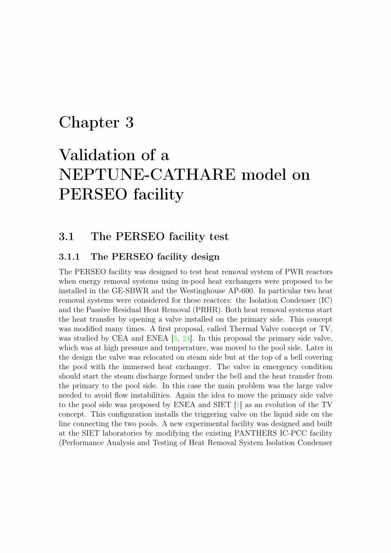
– Passive Containment Condenser). The scheme of the PERSEO (in-pool EnergyRemoval System for Emergency Operation) facility is depicted in Figure 3.1.1. ThePERSEO system mainly consists of a primary and a secondary side. The primaryside contains the pressure vessel and the heat exchanger interconnected by thesteam feed line and a condensate drain line. The secondary pool side consists oftwo pools connected at the top by a steam duct ending with an injector flowinginto the Overall Pool (OP) and at the bottom by a water line with the triggeringvalve. The Heat Exchanger (HX) is contained in the HX pool. The overall poolcontains the water that can be used to cool the primary side.
Primary side pressure MPa 4Primary side temperature K 523.15Primary steam flowrate kg/s 8HX extracted power MW 14HX pool side pressure MPa 0.12HX pool steam flowrate kg/s 6.5
Table 3.1: The main PERSEO test parameters at full power operation during thetransient phase of the test n.9
A test campaign has been conducted on the PERSEO facility in order to verifythe correctness of the proposal and in particular the effectiveness of the decay ofthe heat removal. During operation the pressure vessel is maintained in saturationconditions with a pressure of about 7 MPa which is typical of BWR primarysides or PWR secondary sides for steam generators. The pressure, maintained bysupplying properly de-superheated steam generated from a nearby power station,is kept constant by controlling the steam supply valve. At the same time the waterlevel in the vessel is maintained at the specified value by discharging water throughthe condensate discharge line. At the beginning of the test the HX, the feed lineand the drain line are full of saturated steam. The HX pool, depending on thetest, is full of air or steam and the OP is full of cold water at the nominal level withthe triggering valve closed. Once the system reaches the initial test conditions thetriggering valve opens and the HX pool is flooded by cold water which condensatesthe steam inside the HX tubes with power transfer from the primary side to thepool side. As soon as pool water boiling starts, the steam produced in the HXpool is driven towards the OP through the steam duct. The injector below thewater level contributes to mix the OP water avoiding temperature stratification.The water inside the OP heats up until the boiling point is reached. The steamproduced in the OP flows outside the system at atmospheric pressure throughthe boil-off outlet. When the water level is below the injector no condensation ispresent anymore in the OP and the steam flows outside directly through the boil-off
51

Validation of a NEPTUNE-CATHARE model on PERSEO facility
pipe. The water reserve in the OP decreases according to the heat transfer rate inthe HX pool. During the system operation, the natural circulation which becomesstable on both primary and secondary sides determines the power evacuated bythe system. In some tests, water is discharged from the OP bottom to acceleratethe transient phase with water level decreasing.
3.1.2 PERSEO experimental test 9
Event Time (s)Beginning of the test 0
Triggering valve opening 142 (in 21 s)OP water discharge opening 2790Onset of OP water boiling 3200OP water discharge closure 4840Triggering valve closure 4887 (in 93 s)
End of test 7708
Table 3.2: Chronology of main events characterizing test n.9
Many different tests have been performed during the experimental campaignon the PERSEO facility [13]. Among all of them, test 9 shows the different phasesof a long accidental transient. Therefore we are planning to investigate this testthat should show the performances of the model during the different phases. Test9 starts the operations with total HX pool fill-up. Then, after reaching the boilingconditions, the pool level decreases. This test was devoted to investigate the systemwhen the HX pool is filled up and the thermal regime in both pools is reached.Furthermore, this test studies the effectiveness of the injector in mixing the OPwater and the power and flow regime variation after the OP level decreases belowthe injector outlet. The main PERSEO test parameters at full power operationduring the transient phase are listed in Table 3.1. The chronology of the mainevents characterizing the test is shown in Table 3.2.
The overall behavior of the system is illustrated in Figures 3.2 and 3.3. Afteropening the triggering valve at t = 163 s, the low water level in the HX poolquickly increases close to the top of the tube bundle. The progressive decreasingof the OP level is started by the water discharge from the bottom at t = 2790 s,approximately 400 s before the onset of boiling. The water discharge is stoppedat t = 4840 s, that is 140 s before the complete triggering valve closure. As aconsequence, the OP level drop is terminated in conjunction with the beginningof the decrease of the extracted power which tends to zero at the end of the test.
52

Validation of a NEPTUNE-CATHARE model on PERSEO facility
Figure 3.2: Test 9. Overall pool water level behavior (top) and HX pool relativepressure (bottom)
The power extracted by the HX decreases with the decreasing of the primarysystem pressure. The decreasing is caused by the enhanced pressure losses inthe feed line with consequent reduction of natural circulation of primary massflowrate. Another cause of the decreasing is the lower saturation temperatureresulting in reduced temperature difference between primary and secondary sides.The extracted power is 14 MW and the onset boiling in the OP takes place aroundt = 3200 s. As expected the temperature stratification phenomenon in the OPdisappears as soon as boiling is reached in the pool.
53

Validation of a NEPTUNE-CATHARE model on PERSEO facility
Figure 3.3: Test 9. HX exchanged power (top) and overall pool temperatures(bottom)
3.2 CATHARE-NEPTUNE coupled simulationWe are tempted to analyze the system with the three-dimensional NEPTUNE codebut the complexity of the geometry of the PERSEO facility does not allow this. Forthis reason we may try to simulate only some components. The most interestingcomponents are the overall pool and the injector. In this section we present asimple study with the NEPTUNE code of the overall pool and the injector. Adetailed sketch of the overall pool and the injector is shown in Figures 3.4-3.5
54

Validation of a NEPTUNE-CATHARE model on PERSEO facility
Figure 3.4: PERSEO facility steam duct and liquid line between the pools
with dimensions and geometric details. In order to analyze these components wemust know the input and output mass fluxes together with the inlet temperatures.Again, due to the complexity of the geometry the knowledge of the boundaryconditions of a component can be known only through the use of some mono-dimensional system software applied to the whole system. In order to do this weuse the CATHARE code that will be coupled with the NEPTUNE simulation.We did not perform a full coupling. The full coupling implies that CATHAREand NEPTUNE are solved in separate domains and the CATHARE-NEPTUNEsolutions are iterated until convergence is reached. We use a very weak couplingthat allows first the solution of the CATHARE code over all the domain and thenthe solution of the overall pool and injector components with the NEPTUNE codeusing the previously obtained results as boundary conditions.
The weak coupling between CATHARE and NEPTUNE is sketched in Figure3.6. The boundary conditions needed for this weak coupling between the OP-injector system and the rest of the PERSEO facility are the temperatures andmass flows through the water discharge, water-to-HX-pool, boil off and steam linesections. The OP-injector system may be considered at standard atmosphericpressure. In the OP-injector three fluids are present: steam, water and air, asshown in Figure 3.7. In order to solve the problem with NEPTUNE code we needto enforce boundary conditions. Since the state variables in CATHARE are mono-
55
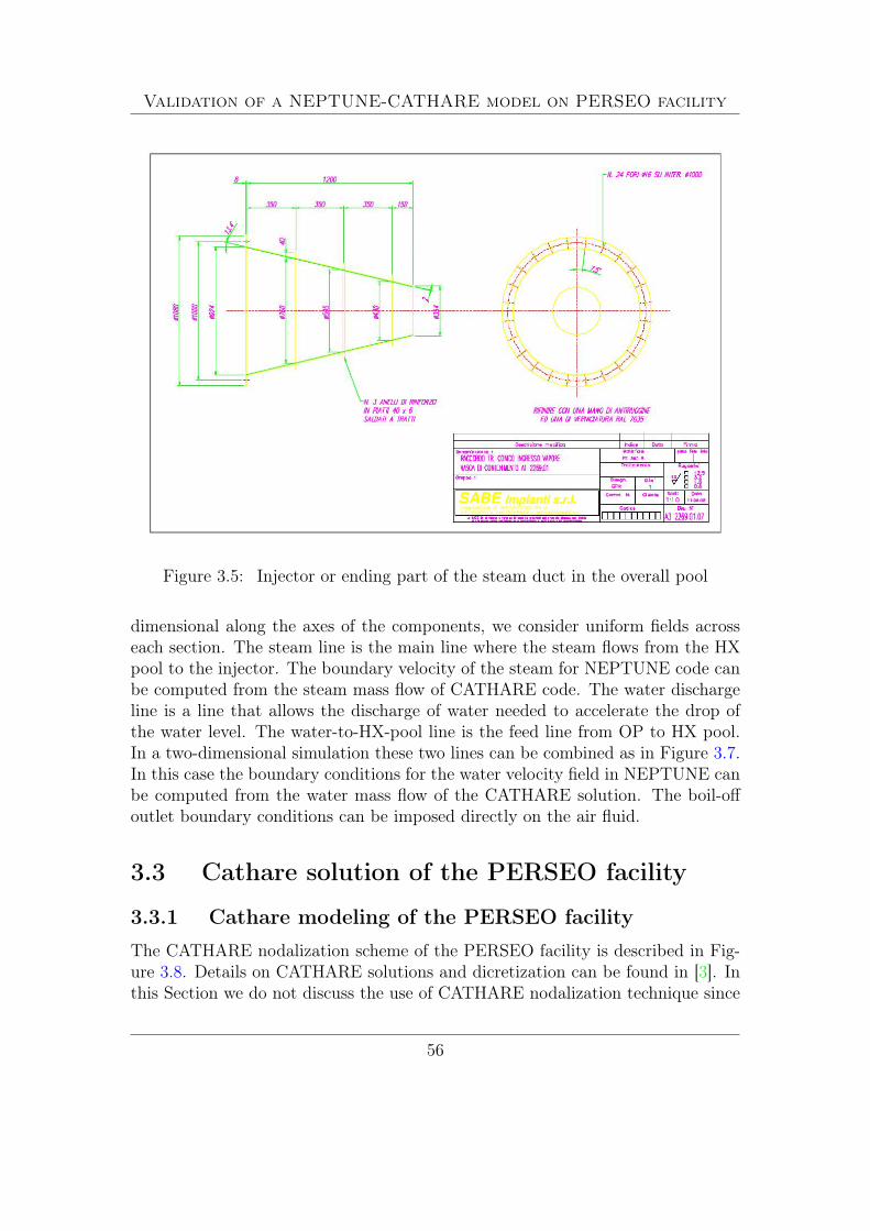
Validation of a NEPTUNE-CATHARE model on PERSEO facility
Figure 3.5: Injector or ending part of the steam duct in the overall pool
dimensional along the axes of the components, we consider uniform fields acrosseach section. The steam line is the main line where the steam flows from the HXpool to the injector. The boundary velocity of the steam for NEPTUNE code canbe computed from the steam mass flow of CATHARE code. The water dischargeline is a line that allows the discharge of water needed to accelerate the drop ofthe water level. The water-to-HX-pool line is the feed line from OP to HX pool.In a two-dimensional simulation these two lines can be combined as in Figure 3.7.In this case the boundary conditions for the water velocity field in NEPTUNE canbe computed from the water mass flow of the CATHARE solution. The boil-offoutlet boundary conditions can be imposed directly on the air fluid.
3.3 Cathare solution of the PERSEO facility
3.3.1 Cathare modeling of the PERSEO facility
The CATHARE nodalization scheme of the PERSEO facility is described in Fig-ure 3.8. Details on CATHARE solutions and dicretization can be found in [3]. Inthis Section we do not discuss the use of CATHARE nodalization technique since
56

Validation of a NEPTUNE-CATHARE model on PERSEO facility
CATHAREInput data
Figure 3.6: Coupling CATHARE-NEPTUNE
Steam Inlet
Boil off
Water to HX pool and discarge
Water
Air
Figure 3.7: Boundary conditions for the overall pool and injector components
57

Validation of a NEPTUNE-CATHARE model on PERSEO facility
Figure 3.8: CATHARE discretization of the PERSEO test 9
the main focus here will be on the NEPTUNE code. The 0-D two-node module(volume) is used to represent the primary vessel, the HX collectors, the HX poollower and upper plenum and the OP (complete mixing). The volumes are inter-connected by axial elements (pipe) representing the HX tube bundle, the waterlines and the steam lines. Axial elements with cross-flow junctions are used tobetter simulate 2-D recirculation within the HX pool and the HX submerging anduncovering during the transient phase. Empirical correlations are used in the sys-tem code in order to reproduce the experimental data. In particular the EPICEcorrelation for boiling heat transfer in the HX pool and the SUPERCLAUDIAcorrelation for direct contact condensation in the OP are implemented in the code[6]. A pressure boundary condition at the HX pool top was kept active for 100 sduring start-up to avoid large numerical instabilities. These numerical instabili-ties are likely generated by natural circulation within the HX pool leading to animmediate strong condensation of steam in the upper plenum when cold water isinjected at the pool bottom. The evaluation of pressure drop through the steaminjector is needed to well reproduce the HX pool relative pressure and thus theoverall system behavior. Therefore, friction losses through the conic-shape injec-tor are calibrated on differential pressure measurements. To this aim, appropriatesingular pressure loss coefficients are taken into account in the injector trying to
58
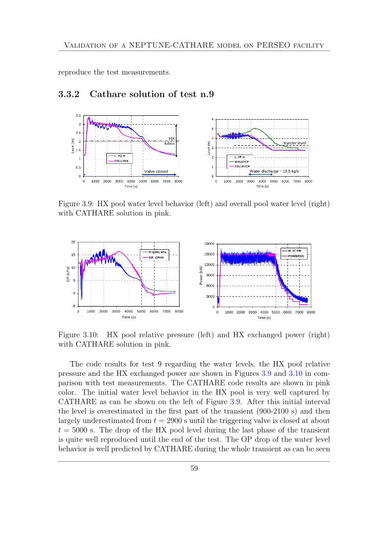
Validation of a NEPTUNE-CATHARE model on PERSEO facility
reproduce the test measurements.
3.3.2 Cathare solution of test n.9
Figure 3.9: HX pool water level behavior (left) and overall pool water level (right)with CATHARE solution in pink.
Figure 3.10: HX pool relative pressure (left) and HX exchanged power (right)with CATHARE solution in pink.
The code results for test 9 regarding the water levels, the HX pool relativepressure and the HX exchanged power are shown in Figures 3.9 and 3.10 in com-parison with test measurements. The CATHARE code results are shown in pinkcolor. The initial water level behavior in the HX pool is very well captured byCATHARE as can be shown on the left of Figure 3.9. After this initial intervalthe level is overestimated in the first part of the transient (900-2100 s) and thenlargely underestimated from t = 2900 s until the triggering valve is closed at aboutt = 5000 s. The drop of the HX pool level during the last phase of the transientis quite well reproduced until the end of the test. The OP drop of the water levelbehavior is well predicted by CATHARE during the whole transient as can be seen
59

Validation of a NEPTUNE-CATHARE model on PERSEO facility
Figure 3.11: Overall pool temperatures (left) and HX tube wall temperature(right) with CATHARE solution is pink.
in Figure 3.9 on the right. The oscillatory behavior of the OP water level observedin the test before boiling might be caused by sudden steam condensation at the in-jector outlet, inducing fluctuations at the pool free surface. The lack of oscillationsin the calculated OP level occurs in conjunction with much smaller fluctuations inthe HX pool level and in the HX relative pressure values calculated by the code inthe interval t = 500-3000 s as shown on the left of Figure 3.10. In this figure weremark that the large HX pool relative pressure overestimation between t = 2700– 5000 s is consistent with the corresponding HX pool level underestimation. Asexpected, the differences with previous results become significant only after onsetof OP water boiling around t = 3200 s. The computed power, shown on the rightof Figure 3.10, is 15 MW while the experimental extracted power is 14 MW. Thepower drop predicted by the code after triggering valve closure at about t = 5000s is slightly quicker than the one observed in the test. The onset of boiling in theOP, which takes place around t = 3200 s, is well captured by the code as shown onthe left of Figure 3.11. The onset of HX tube wetting is well predicted by the code(see Figure 3.11 on the right) but the HX tube wall temperature is over predictedunder wetting conditions.
3.3.3 Boundary conditions for NEPTUNE
From the CATHARE solution we can compute the boundary conditions for theNEPTUNE code. Since the state variables in CATHARE are mono-dimensionalwe consider uniform fields across every section. In Figure 3.12 we report the steammass flow through the steam line which is the main line where the steam from theHX pool comes to the injector. On the left of Figure 3.13 we show the CATHAREsolution of the water discharge line, which is a line that allows the discharge ofwater needed to accelerate the drop of the water level. On the right of this Figure,
60
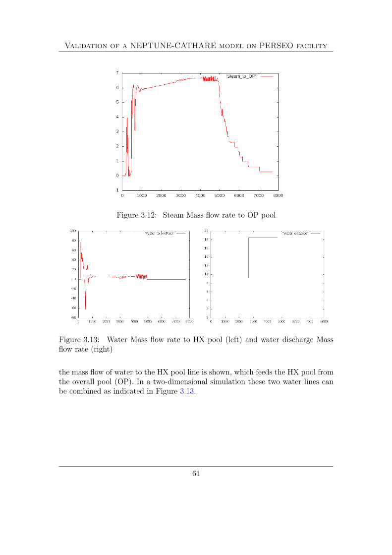
Validation of a NEPTUNE-CATHARE model on PERSEO facility
Figure 3.12: Steam Mass flow rate to OP pool
Figure 3.13: Water Mass flow rate to HX pool (left) and water discharge Massflow rate (right)
the mass flow of water to the HX pool line is shown, which feeds the HX pool fromthe overall pool (OP). In a two-dimensional simulation these two water lines canbe combined as indicated in Figure 3.13.
61

Validation of a NEPTUNE-CATHARE model on PERSEO facility
CASES
SIMUL MESH
DATA
RESU
SRC
SCRIPTS
Figure 3.14: Directory of the NEPTUNE code
3.4 NEPTUNE on CRESCO set up simulation
3.4.1 Code setup
The NEPTUNE project provides a two-phase flow thermal hydraulics softwarefor two/three-dimensional computations of the main components of nuclear reac-tors: cores, steam generators, condensers, heat exchangers. NEPTUNE supportsfrom one to twenty fluid fields (or phases) and includes thermodynamic laws forwater/steam flows. It is based on advanced physical models (two-fluid equationscombined with interface area transport and two-phase turbulence) and on the cell-centered type finite volume method which can use meshes with all types of celland nonconforming connections.
The NEPTUNE code is located on CRESCO-ENEA GRID in the directory
/afs/enea.it/project/fissicu/soft/Neptune
NEPTUNE requires a specific structure for the configuration and input files. Thesimulation directory is denoted as SIMUL. We can therefore create a CASES directoryand put all NEPTUNE simulations inside. To create a folder tree for the studySIMUL we use the available script
$ buildcase_nept -study SIMUL
62

Validation of a NEPTUNE-CATHARE model on PERSEO facility
This generates the correct directory structure. There is a MESH directory, whereall the meshes are stored. Inside this directory, the case SIMUL will have its owndirectory as
CASES+-- CASE1+-- SIMUL + working directory...+-- MESH
As shown in Figure 3.14, the working directory SIMUL contains the four sub-directories
- DATA, where the XML configuration file is stored;
- RESU, that is used for the outputs;
- SCRIPTS, that hosts the execution scripts;
- SRC, in which we can put some additional source file.
Once the PATH is set the NEPTUNE GUI starts with the command
$ neptune
At the moment not all the libraries required for the GUI are available in theCRESCO architecture and therefore we run the NEPTUNE GUI on a simpleworkstation through which we create the param file. Then we copy this file onCRESCO in the appropriate position and we run NEPTUNE code in batch runningmode. In order to execute the application in a shell we set the environment by usingthe script neptune_env that is located in the bin directory. The recommendedway to run NEPTUNE from command line is to use the runcase script. There isa template available inside the directory
/afs/enea.it/project/fissicu/soft/Neptune/data
One has to enter the SCRIPTS directory inside the case under analysis and run
$ ./runcase
On the top of the runcase template the configuration options for LSF are listed.We set
63

Validation of a NEPTUNE-CATHARE model on PERSEO facility
...BSUB -J Test9BSUB -n 1BSUB -oo journal_oBSUB -eo journal_e
....
where the option -J sets the job name Test9, -n the number of processors 1, -oothe file journal_o for the standard output and -eo the error output journal_e.Once the script is ready the command
$ bsub < runcase
starts the batch execution. Further information on batch commands are availablein [2].
3.4.2 Initial, boundary condition and physical property files
NEPTUNE requires a dataset file, named param, and a mesh file. The mesh filemay have the UNV or MED format. In our implementation NEPTUNE is not ableto read the MED format and therefore we must use the UNV format files for themesh geometry. The geometry chosen for this first approach is the two-dimensionalgeometry shown in Figure 3.7. This geometry includes the injector and the pooland considers the water discharge and the water OP-to-HX line as a unique line.The param file contains all the physical properties and boundary conditions. Asshown in Figure 3.15 in the overall pool and the injector system we have threefluids: water (eau), steam (vapeur) and air (air). The physical properties ofthese three fluids are taken as in Table 3.3. The label “Cathare table” refers to
fluid T (K) ρ(Kg/m3) µ(Pa s) Cp(W/m3K)steam 297.75 Cathare table Cathare table Cathare tablewater 297.75 Cathare table Cathare table Cathare tableair gas law 2 2× 10⁻⁵ 1006
Table 3.3: Fluid and flow properties selected for PERSEO test 9
an internal database that correlates pressure and temperature of water and steamwith the physical properties. The reference temperature and pressure for all thephases are the room temperature T = 297.75 K and standard pressure p = 1 atmrespectively. The turbulence model in water is the Rij − ε model recommended byNEPTUNE. We set the mixing length model for air, while no turbulence model isset in the steam component. On the wall we use friction boundary conditions for
64

Validation of a NEPTUNE-CATHARE model on PERSEO facility
Figure 3.15: Physical properties.
water and air and zero velocity normal derivative for steam. The Ishii drag modelfor the steam phase is used.
As shown in Figure 3.16 the boundary consists of seven regions: steam inlet,boil-off, water line, injector wall, top pool wall, pool wall and symmetry boundaryregion. The names are self describing; the steam inlet is the inlet of the steam inthe injector and the boil-off is the outlet boundary at the top of the pool. Theinjector wall, top pool wall and pool wall appear in Figure 3.16 as a unique columnsince all these regions can be considered as standard walls with the same kind ofboundary conditions. The mesh imported by NEPTUNE is three-dimensionalwith unitary thickness. Since in finite volume discretization, fields are constant inthe cell and located at the center of the cell the symmetry boundary conditionsare needed to simulate two-dimensional geometries with three-dimensional meshes.For details see [19]. On the steam inlet region only steam can enter with directionnormal to the surface and mass flux defined in the appropriate file as a function of
65

Validation of a NEPTUNE-CATHARE model on PERSEO facility
Figure 3.16: Boundary conditions.
time by the previously solved CATHARE solution. The temperature condition isset to Sat option which denotes the saturation temperature at the correspondingpressure. The boil-off boundary condition is the standard outflow condition forair while water and steam are not allowed to exit. Concerning the water lineboundary condition, temperature is fixed to room temperature and mass flow isimposed through a file as a function of time. At the wall we enforce standardturbulent boundary conditions for water and air.
Many numerical schemes and options can be activated in NEPTUNE. In thissimulation we use the Special Modules option which allows to enable special fea-tures of the two-phase flow. We enable the option water/steam module whichallows the use of Cathare table for water/steam systems. We leave this option asrecommended in the tutorial. In the section scalar of the NEPTUNE code we setthree scalars, the total enthalpies for each fluid. Two scalars are enabled automat-ically when the water/steam module is selected in Special modules, i.e. the two
66

Validation of a NEPTUNE-CATHARE model on PERSEO facility
Figure 3.17: Overall pool temperature measurement positions.
67

Validation of a NEPTUNE-CATHARE model on PERSEO facility
Figure 3.18: Overall pool temperatures for different probes.
total enthalpies for water and steam. The state variable is not therefore the tem-perature but the total enthalpy, from which one can compute the correspondingtemperature by using the appropriate thermodynamical law.
In this test we would like to reproduce temperature behaviors from the PERSEOtest. In Figure 3.17 we have a layout of the overall pool temperature measure-ment positions. We are going to study the computed temperatures at the probepositions denoted by TP6, TP8, TP23 and TP25. The experimental results arereported in Figure 3.18. The exact location of the probes can be found in Table
position X Y Z Codeoverall pool under the Injector 500 3400 2195 TP006overall pool under the Injector 500 3400 1795 TP007overall pool under the Injector 500 3400 1195 TP008
overall pool central area 1910 3745 2695 TP021overall pool central area 1910 3745 2195 TP023overall pool central area 1910 3745 1195 TP025overall pool central area 1910 3745 50 TP028overall pool central area 3540 3745 2695 TP030overall pool central area 1910 3745 2495 TP022
Table 3.4: Exact locations (in mm) of the probes for temperature measurementswith respect to the reference frame indicated in Figure 3.17.
3.4. The NEPTUNE code has a probe system that allows the monitoring of any
68

Validation of a NEPTUNE-CATHARE model on PERSEO facility
point in space and time.In this simulation we must introduce some user subroutines. To compile them
it is necessary to copy the corresponding file from the USERS directory into the SRCdirectory. The boundary conditions are imposed by using the CATHARE solution.In order to impose the boundary conditions as a function of time one must modifythe file /src/usclim.F. On the injector inlet boundary, the mass flow functionm(t) for phase 1 (steam) over the interval t ∈ [1.43E + 02, 1.68E + 02] is given by
m(t) =−(−5952.98 + 74.3234 t− 0.228571 t2)
54.7. (3.1)
By using the FORTRAN language we write it as
IF ((TTCABS .GE. 1.43E+02)& .AND. (TTCABS .LT. 1.68E+02)) THEN
DEBCL(1,2)=-FACT_W*( -5952.98+74.3234*TTCABS-0.228571& *TTCABS*TTCABS)ENDIF
Here, DEBCL(j,α) is the mass flux on boundary j (steam inlet boundary is denotedby 1 in order) for phase α (steam is phase 2). Time is denoted in this file by TTCABS.
The initial conditions must be defined in the file /src/usiniv.F. Since in theOP we start with a water level of 4.5 m and air above with no steam we mustwrite
DO IEL = 1,NCELIF (XYZCEN(1,IEL) .GT. 4.5 ) THENRTP(IEL,IALPR(2)) = 1.D0RTP(IEL,IALPR(1)) = 0.D0RTP(IEL,IALPR(3)) = 0.D0
ELSERTP(IEL,IALPR(1)) = 1.D0RTP(IEL,IALPR(2)) = 0.D0RTP(IEL,IALPR(3)) = 0.D0
ENDIFENDDO
The RTP(e,α) function gives the value of the volume fraction in the element ewith phase α.
The physical laws and properties must be added in the file /src/usphysv.F.The air needs the gas law and therefore we must add
DO IEL=1,NCEL
69

Validation of a NEPTUNE-CATHARE model on PERSEO facility
H3=RTPA(IEL,IENTHT(3))& -0.5*(RTPA(IEL,IU(3))**2& +RTPA(IEL,IV(3))**2& +RTPA(IEL,IW(3))**2 )
GAM=1.4PROPHY(IEL,IROM(3))=GAM/(GAM-1.)*RTPA(IEL,IPR)/H3PROPHY(IEL,ITEMPK(3))=H3/PROPHY(IEL,ICP(3))
ENDDO
where we define the air temperature as T = h/cp and the expression for theenthalpy. Details can be found in [2].
3.5 NEPTUNE simulation of PERSEO Test 9
1 2 3 4
Figure 3.19: Chronology of the temperature main events for the probe TP6
If one observes the chronology of the temperature main events for test 9 asreported in Figure 3.19, one can divide the experiment evolution into four parts:
1. Beginning;
2. Temperature stratification (pool heating);
70
Validation of a NEPTUNE-CATHARE model on PERSEO facility
3. Steam injection (pool boiling);
4. Injection above water level.
The interval of time of each period is summarized in Table 3.5.
n Description Time (s)1 Beginning of the test 0 -5002 pool heating 500-32003 pool boiling 3200-42004 Low water level 4200-7700
Table 3.5: Chronology of the Temperature main events
In the next section we analyze each of these stages.
3.5.1 Beginning of the test
During the initial part of the simulation the pool temperature is low. At t = 0 theinitial conditions of the system are reported in Table 3.6. The boundary condi-
Parameter Unit ValueOP water level m 4.50
OP water temperature oC 24.5HX pool water level m 1.222
HX pool water temperature oC 47
Table 3.6: Initial conditions of OP and HX pool.
tions for NEPTUNE during the time interval 0−500 s as computed by CATHAREare shown in Figures 3.20-3.21. In Figure 3.20 and on the left of Figure 3.21 thewater mass flow rate from OP to HX pool and the water discharge mass flowrate are shown, respectively. These two flows are set as boundary conditions overthe boundary that defines the water line. In order to do this we interpolate theCATHARE values at the time nodes and write the resulting interpolating func-tions on the file uslimv.F as described in the previous section. The steam massflow rate from the HX pool to the OP is reported on the right of Figure 3.21. Thismass flow generates the velocity at the steam inlet. Since the CATHARE solutionprovides a unique scalar value, the velocity profile is assumed to be constant.During the interval t ∈ [0, 143] s all the boundary mass flow rates are set to zeroso that the system can reach a stable condition. At t = 150 s the water level of
71

Validation of a NEPTUNE-CATHARE model on PERSEO facility
Triggering valve opening
Figure 3.20: Water mass flow rate to HX pool over the time interval [0 − 500]scomputed from CATHARE simulation.
Figure 3.21: Water discharge mass flow rate and steam mass flow rate to overallpool over the time interval [0− 500]s computed from CATHARE simulation.
the simulation is almost everywhere uniform as one can see in Figure 3.22. Duringthe interval t ∈ [143 − 204] s a water level adjustment occurs. As one can seein Figure 3.20, the water moves from the overall pool to the HX pool since thecorresponding level in the HX pool is low due to steam formation. The resultinglevel in the OP is shown in Figure 3.23. The water levels in the injector andin the overall pool are different due to the steam pressure. In the final intervalt ∈ [204 − 500] s the steam enters the injector with a significant mass flow rate
72
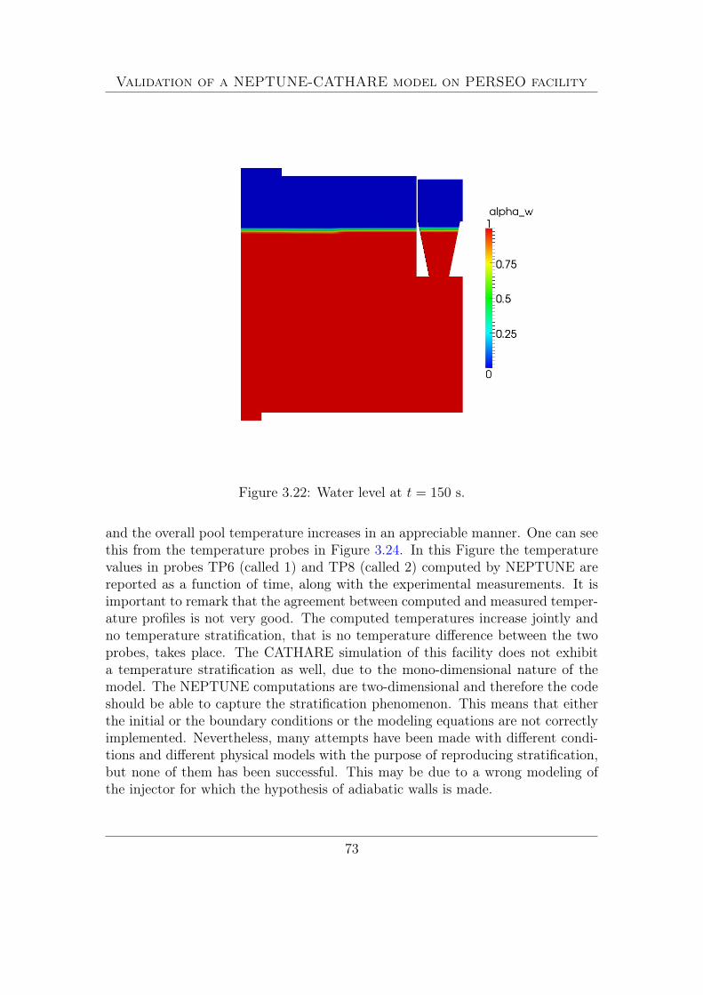
Validation of a NEPTUNE-CATHARE model on PERSEO facility
Figure 3.22: Water level at t = 150 s.
and the overall pool temperature increases in an appreciable manner. One can seethis from the temperature probes in Figure 3.24. In this Figure the temperaturevalues in probes TP6 (called 1) and TP8 (called 2) computed by NEPTUNE arereported as a function of time, along with the experimental measurements. It isimportant to remark that the agreement between computed and measured temper-ature profiles is not very good. The computed temperatures increase jointly andno temperature stratification, that is no temperature difference between the twoprobes, takes place. The CATHARE simulation of this facility does not exhibita temperature stratification as well, due to the mono-dimensional nature of themodel. The NEPTUNE computations are two-dimensional and therefore the codeshould be able to capture the stratification phenomenon. This means that eitherthe initial or the boundary conditions or the modeling equations are not correctlyimplemented. Nevertheless, many attempts have been made with different condi-tions and different physical models with the purpose of reproducing stratification,but none of them has been successful. This may be due to a wrong modeling ofthe injector for which the hypothesis of adiabatic walls is made.
73

Validation of a NEPTUNE-CATHARE model on PERSEO facility
Figure 3.23: Water level at t = 204 s.
3.5.2 Temperature stratification
During the interval t ∈ [500 − 3200] s the pool temperature increases until itreaches boiling. For the time interval under study, the steam mass flow rate tothe overall pool is shown in Figure 3.25; the water mass flow rates to the HXpool and to the discharge line are reported in Figure 3.26 on the left and rightrespectively. In two-dimensional geometry these two flows may be added to definethe boundary condition for the water line. The NEPTUNE simulation shows agreat mixing with no temperature stratification. The mixing is generated by thecyclic behavior of the injector. The injector is periodically filled with steam. Thesteam cannot enter the pool and condensates near the injector outlet. The steampressure pushes the water down till the level goes below the injector. The steammixes with water and the water enters the injector again. The steam condensatesand the water is sucked until it fills the injector almost completely. Then the cyclerepeats again. This can be seen in Figures 3.27-3.28. On the top of Figure 3.27 wesee that the injector is filling with steam which then pushes the water level down(Figure 3.27 on the bottom). On the top of Figure 3.28 the water level drops
74

Validation of a NEPTUNE-CATHARE model on PERSEO facility
Figure 3.24: Computational and experimental temperature profiles in probes TP6(1) and TP8 (2) as a function of time.
Figure 3.25: Steam mass flow rate to overall pool over the time interval [500 −3000]s defined from CATHARE simulation
down and water and steam mix quickly to fill again the injector completely asshown on the bottom of Figure 3.28. The resulting temperatures at the probes is
75
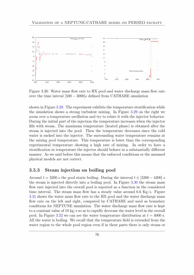
Validation of a NEPTUNE-CATHARE model on PERSEO facility
Water discarge opening
Figure 3.26: Water mass flow rate to HX pool and water discharge mass flow rateover the time inteval [500− 3000]s defined from CATHARE simulation
shown in Figure 3.29. The experiment exhibits the temperature stratification whilethe simulation shows a strong turbulent mixing. In Figure 3.29 on the right wezoom over a temperature oscillation and try to relate it with the injector behavior.During the initial part of the injection the temperature increases when the injectorfills with steam. The maximum temperature (heated phase) is obtained after thesteam is injected into the pool. Then the temperature decreases since the coldwater is sucked into the injector. The surrounding water temperature remains atthe mixing pool temperature. This temperature is lower than the correspondingexperimental temperature showing a high rate of mixing. In order to have astratification in temperature the injector should behave in a substantially differentmanner. As we said before this means that the enforced conditions or the assumedphysical models are not correct.
3.5.3 Steam injection on boiling pool
Around t = 3200 s the pool starts boiling. During the interval t ∈ [3200− 4200] sthe steam is injected directly into a boiling pool. In Figure 3.30 the steam massflow rate injected into the overall pool is reported as a function in the consideredtime interval. The steam mass flow has a steady value around 6.6 Kg/s. Figure3.31 shows the water mass flow rate to the HX pool and the water discharge massflow rate on the left and right, computed by CATHARE and used as boundaryconditions for NEPTUNE simulation. The water discharge mass flow rate is keptto a constant value of 18 kg/s so as to rapidly decrease the water level in the overallpool. In Figure 3.32 we can see the water temperature distribution at t = 4000 s.All the water is boiling. We recall that the temperature field is extended from thewater region to the whole pool region even if in these parts there is only steam or
76

Validation of a NEPTUNE-CATHARE model on PERSEO facility
Figure 3.27: Steam entering the injector (top) and injection of steam into water(bottom)
77

Validation of a NEPTUNE-CATHARE model on PERSEO facility
Figure 3.28: Steam and water mixing (top) and inverse flow (bottom)
78

Validation of a NEPTUNE-CATHARE model on PERSEO facility
Water discarge opening
Heated phase
Direct flow Inverse flow
Heated phase
Direct flow Inverse flow
Figure 3.29: Temperature of the probes TP6 (red) and TP8 (green) from experi-ment and NEPTUNE computation (blue and violet) and zoom of the temperatureoscillations
Figure 3.30: Steam mass flow rate to overall pool over the time interval [3200 −4200]s defined from CATHARE simulation.
air. On the top of Figure 3.33 we can see the injection of steam into the boilingpool when the water level is below the injector outlet. In this case the condensationis minimal and all the steam goes above the level of the water pool as shown inFigure 3.33 on the bottom. Condensation may take place in some areas of thepool, especially near the boil-off where the cold air may condensate the saturatedsteam.
79
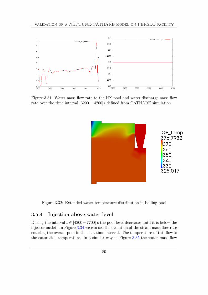
Validation of a NEPTUNE-CATHARE model on PERSEO facility
Figure 3.31: Water mass flow rate to the HX pool and water discharge mass flowrate over the time interval [3200− 4200]s defined from CATHARE simulation.
Figure 3.32: Extended water temperature distribution in boiling pool
3.5.4 Injection above water level
During the interval t ∈ [4200−7700] s the pool level decreases until it is below theinjector outlet. In Figure 3.34 we can see the evolution of the steam mass flow rateentering the overall pool in this last time interval. The temperature of this flow isthe saturation temperature. In a similar way in Figure 3.35 the water mass flow
80

Validation of a NEPTUNE-CATHARE model on PERSEO facility
Figure 3.33: Steam injection on boiling pool (top) and steam release to the watersurface (bottom)
81

Validation of a NEPTUNE-CATHARE model on PERSEO facility
Figure 3.34: Steam mass flow rate to overall pool over the time interval [4200 −7700]s defined from CATHARE simulation.
Water discarge closing
Figure 3.35: Water mass flow rate to the HX pool and water discharge mass flowrate over the time interval [4200− 7700]s defined from CATHARE simulation.
rate to the HX pool and the water discharge mass flow rate are shown on the leftand right respectively. The water discharge mass flow rate is kept constant to 18.8kg/s till about t = 4700 s and then it is set to zero when the water discharge lineis closed. The temperature on this boundary region is room temperature. Withthese boundary conditions we can compute the velocity and temperature profilesof all the phases. On the top of Figure 3.36 we can see the steam injection intothe water pool. In Figure 3.36 on the bottom the steam is injected above thewater level. There is no mixing with water and the energy is released directly to
82

Validation of a NEPTUNE-CATHARE model on PERSEO facility
Figure 3.36: Steam injection above the water level.83

Validation of a NEPTUNE-CATHARE model on PERSEO facility
the pool surface. From the pool surface the steam mixes with the air and then itgoes out of the system through the boil-off boundary. In this case we believe thatthe NEPTUNE code simulates pretty well the heat exchange between the differentphases.
84

Chapter 4
Validation of TRIO_U interfacemodel on bubble detachment
4.1 Set up of the TRIO_U codeThis section is devoted to a simple validation of the TRIO_U code. With TRIO_Uwe propose a three-dimensional simulation of a bubble detaching from a heatedwall in pool boiling configuration. Trio_U was developed at the Laboratory ofModeling and Software Development of the Directorate of Nuclear Energy of theCEA with the specific purpose of studying two-phase flows with interfaces [34, 35,36]. The two-phase model is based on the Navier-Stokes equations coupled with anadvection equation for the phase. Since the phases are assumed to be immisciblethe knowledge of the phase is related to the tracking of the interface. The locationof the interface is defined by a set of markers that are advected by the velocityfield.
In order to start the TRIO_U code on CRESCO-ENEA GRID we must setthe TRIO_U environment, the mesh grid and the file data with the physical andnumerical parameters. The TRIO_U platform is located on CRESCO-ENEAGRID in the directory
/afs/enea.it/project/fissicu/soft/Triou
The TRIO_U application will be run in console mode. From console one mustfirst set the access to the bin directory
/afs/enea.it/project/fissicu/soft/bin
by executing the script
$ source pathbin.sh
Validation of TRIO_U interface model on bubble detachment
Once the bin directory is in the PATH environment variable, all the programs ofthe platform can be launched from anywhere. The command needed to start theTRIO_U application is
$ triou
The dataset file must be labeled with the extension .data and contains allthe parameter values and all the options. The options are introduced in the codethrough keywords. For example, consider the Lire keyword. The interpreterallows the Lire object to be defined in various ways:
a) with brackets
Lire object1{....}
In this case this keyword provides the object object1 defined between the braces;b) by command line
Lire_fichier object1 namefile
The keyword Lire_fichier indicates that the object object1 be read in the filenamefile. This is notably used when the mesh of the calculation domain hasalready been generated and the mesh contains the file namefile;
c) with _bin
Lire_fichier_bin object1 namefile
for an unformatted file.For all the keywords one can read the TRIO_U tutorial inside the doc directory
which is located in
/afs/enea.it/project/fissicu/soft/Triou/doc
We are planning to consider a bubble in a simple three-dimensional rectangu-lar domain. Since this is a very simple domain we generate the mesh with theTRIO_U internal generator.
In order to do this we need to include the commands for mesh generation inthe data file. These commands can be written as
86

Validation of TRIO_U interface model on bubble detachment
dimension 3domaine domain# Mesh description #Mailler domain{ pave pave1{origine 0. 0. 0.longueurs 1. 1. 1.nombre_de_noeuds 51 51 51
}{bord paroi X = 0. 0. <= Y <= 1. 0. <= Z <= 1.bord haut Z = 1. 0. <= X <= 1. 0. <= Y <= 1.bord bas Z = 0. 0. <= X <= 1. 0. <= Y <= 1.bord paroi X = 1. 0. <= Y <= 1. 0. <= Z <= 1.bord paroi Y = 0. 0. <= X <= 1. 0. <= Z <= 1.bord paroi Y = 1. 0. <= X <= 1. 0. <= Z <= 1.}}transformer dom x*0.002-0.001 y*0.002-0.001 z*0.002
The first line indicates the use the three-dimensional coordinate system. Thedomain is described in the Mailler block which consists of two blocks. The firstblock describes the origin coordinate and the number of nodes. The second blockdefines the geometrical boundary and its labeling. The domain is then transformedwith the command transformer to fit the dimension of the bubble.
The properties of the fluid are assigned inside the same file. We have threeblocks: fluid, gas and fluid-gas. These blocks are reported below
Fluide_Incompressible eauLire eau{
mu champ_uniforme 1 70.e-6rho champ_uniforme 1 610lambda champ_uniforme 1 461.e-3cp champ_uniforme 1 8270
}
Fluide_Incompressible airLire air{
87

Validation of TRIO_U interface model on bubble detachment
mu champ_uniforme 1 22.e-6rho champ_uniforme 1 100lambda champ_uniforme 1 111.e-3cp champ_uniforme 1 11000
}
Fluide_diphasique fluideLire fluide{
fluide1 eaufluide0 airsigma constant 0.002chaleur_latente constant -50000
}
The properties of water, steam (gas) and the water-steam interface can be changeddepending on the problem.
In Trio_U there is a specific module called Discontinuous Front TrackingProblem to solve multiphase problems; this module is recalled by the keywordProbleme_ft_Disc_gen. The equations required to solve the detachment of thebubble from a plain surface are three and one must provide a name identificationfor each of them. The three equations are:
• the momentum equation, i.e. the Navier-Stokes equation, which is referredto as Navier_Stokes_ft_Disc;
• an interface equation referring to the interface between two fluids, indicatedby Transport_Interfaces_ft_Disc;
• the temperature equation for a phase, i.e. the energy equation; the keywordfor this equation is Convection_diffusion_temperature_ft_disc.
The previous equations need to be associated with an object of type
Probleme\_ft\_Disc\_gen
in the Trio_U language this instruction is provided by the keyword Associer.The list of equations in the .data file looks as follows:
Probleme_ft_Disc_gen pbNavier_stokes_FT_disc hydrauliqueTransport_interfaces_FT_disc interf
88

Validation of TRIO_U interface model on bubble detachment
Convection_diffusion_temperature_ft_disc thermiqueAssocier pb hydrauliqueAssocier pb thermiqueAssocier pb interf
There are different output file formats:- name.lml: standard storage file for post-processing. The .lml format files
allow the results to be viewed with Data Visualizer or AVS Express;- name.lata: this is similar to the .lml format but comprises several files;- name.ijk: this outputs the results in the form of tables;- name.tv: to be used with the freeware VisIt viewing tool;- name.son: standard storage files for physical values measured by probes
located by the user in the calculation domain. This file can be read by the Gnuplotapplication.
We intend to print the temperature, velocity, pressure and interface fields with.lata format. To this purpose we write a block in the .data file as follows:
Postraitement_ft_lata post1{dt_post 0.005nom_fichier lata/postchamps elements
{indicatrice_interftemperature_thermiquevitessepressiontemperature_mpoint}
interfaces interf{champs sommets { courbure }}
}
4.2 Numerical results
4.2.1 Simulation of bubble detachment in pool boiling
The boiling simulation is carried out in a three-dimensional rectangular domainwith standard water-steam data. The initial temperature and the corresponding
89

Validation of TRIO_U interface model on bubble detachment
q
Tg
Figure 4.1: Constant heat flux boundary condition on the bottom wall
density are linear from the bottom to the top of the domain. The top of the bound-ary is kept at 10o C less than the bottom which is at the saturation temperature.Symmetry conditions are considered as boundary conditions on the other sides ofthe three-dimensional domain. For the velocity field no-slip boundary conditionsare imposed on the top and bottom of the domain and symmetry conditions onthe remaining sides. The gravity is taken into account and a small initial bubbleis located at the center of the bottom surface. The wall is under a constant heatflux as described in Figure 4.1. The bubble temperature starts to grow by heatdiffusion adjacent to the wall until it reaches the saturation value. The change ofphase starts and the bubble grows as shown in Figures 4.2-4.5. When the bubbleachieves the critical volume and the corresponding departure diameter it detachesfrom the wall. This can be seen in Figures 4.5-4.6. The detached bubble is un-stable. If its size is smaller than the critical bubble radius then the bubble risesup and its diameter decreases. In this case the bubble disappears before reachingthe upper boundary. In our simulation the bubble is stable and large enough suchthat a bubble collapse is avoided. As one can see in Figures 4.7-4.9, after the de-tachment the bubble rises and changes its shape till it reaches the upper boundaryof the domain.
4.2.2 Bubble diameter as a function of gravity
In this section we study the diameter of the bubble at departure as a functionof gravity. From the previous simulation we can determine the diameter of thebubble at departure by changing the gravity constant g. From static force balanceone expects that the bubble departure diameter Dd satisfies the following relation
Dd = A/√g (4.1)
where A is a constant. In order to match the static theoretical result in (4.1)
90

Validation of TRIO_U interface model on bubble detachment
Figure 4.2: Simulation of bubble detachment from a wall in pool boiling (1)
Figure 4.3: Simulation of bubble detachment from a wall in pool boiling (2)
Figure 4.4: Simulation of bubble detachment from a wall in pool boiling (3)
91
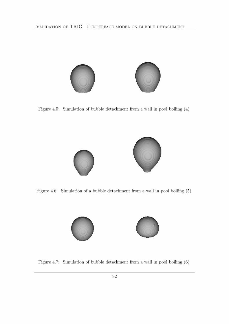
Validation of TRIO_U interface model on bubble detachment
Figure 4.5: Simulation of bubble detachment from a wall in pool boiling (4)
Figure 4.6: Simulation of a bubble detachment from a wall in pool boiling (5)
Figure 4.7: Simulation of bubble detachment from a wall in pool boiling (6)
92

Validation of TRIO_U interface model on bubble detachment
Figure 4.8: Simulation of bubble detachment from a wall in pool boiling (7)
Figure 4.9: Simulation of bubble detachment from a wall in pool boiling (8)
93

Validation of TRIO_U interface model on bubble detachment
30 40 50 60 70 80 90g (m/s^2)
1
1.2
1.4
1.6
1.8
2
D (
mm
)
Figure 4.10: Bubble diameter at departure as a function of gravity g.
we perform several computations with a fixed contact angle of 60o and differentgravity g ranging from 30 to 100m/s2. In order to determine the bubble diameterwe consider the two instants immediately before and after the actual release of thebubble and we compute the bubble departure volume as an average of the two.Assuming an approximate spherical form we can compute the diameter based onthe bubble volume. We fit the computational results with the function
f(g) = a gb (4.2)
with a and b constants to be determined. The best fit gives a = 9.49 and b = −0.49.The results are shown in Figure 4.10. The circles represent the simulation resultsand the solid line is the theoretical prediction in (4.1). If we want to fit the datawith b = −0.5 as suggested by (4.1) then the best result is obtained for a = 10.02.The result are pretty good especially if one takes into account that (4.1) is obtainedin static conditions [17, 7, 12, 18].
94

Validation of TRIO_U interface model on bubble detachment
0.03 0.04 0.05 0.06 0.07 0.08sigma (N/m)
1
1.2
1.4
1.6
1.8
2
D (
mm
)
Figure 4.11: Bubble diameter at departure as a function of surface tension sigma.
4.2.3 Bubble diameter as a function of surface tension
Here we study the diameter of the bubble at departure as a function of surface ten-sion σ. From static force balance one expects that the bubble departure diameterDd satisfies a function of σ as
Dd = B√σ (4.3)
where B is a constant. In order to match the static theoretical result in (4.3)we perform several computations with a fixed contact angle of 60o and differentsurface tensions σ ranging from 0.03 to 0.08 N/m. We can compute the bubblevolume at departure as before and therefore obtain the diameter, by assuming anapproximate spherical form. We fit the computational results with the function
f(σ) = c σd (4.4)
with c and d some constants to be defined. The best fit gives f(σ) = c σd =5.17535σ0.432545. The results are shown in Figure 4.11. The circles represent thesimulation results and the solid line is the theoretical prediction in (4.3). If wewant to fit the data with d = 0.5 as suggested by (4.3) then the best result isobtained for c = 6.23. The numerical results are in good agreement with thetheoretical predictions.
95
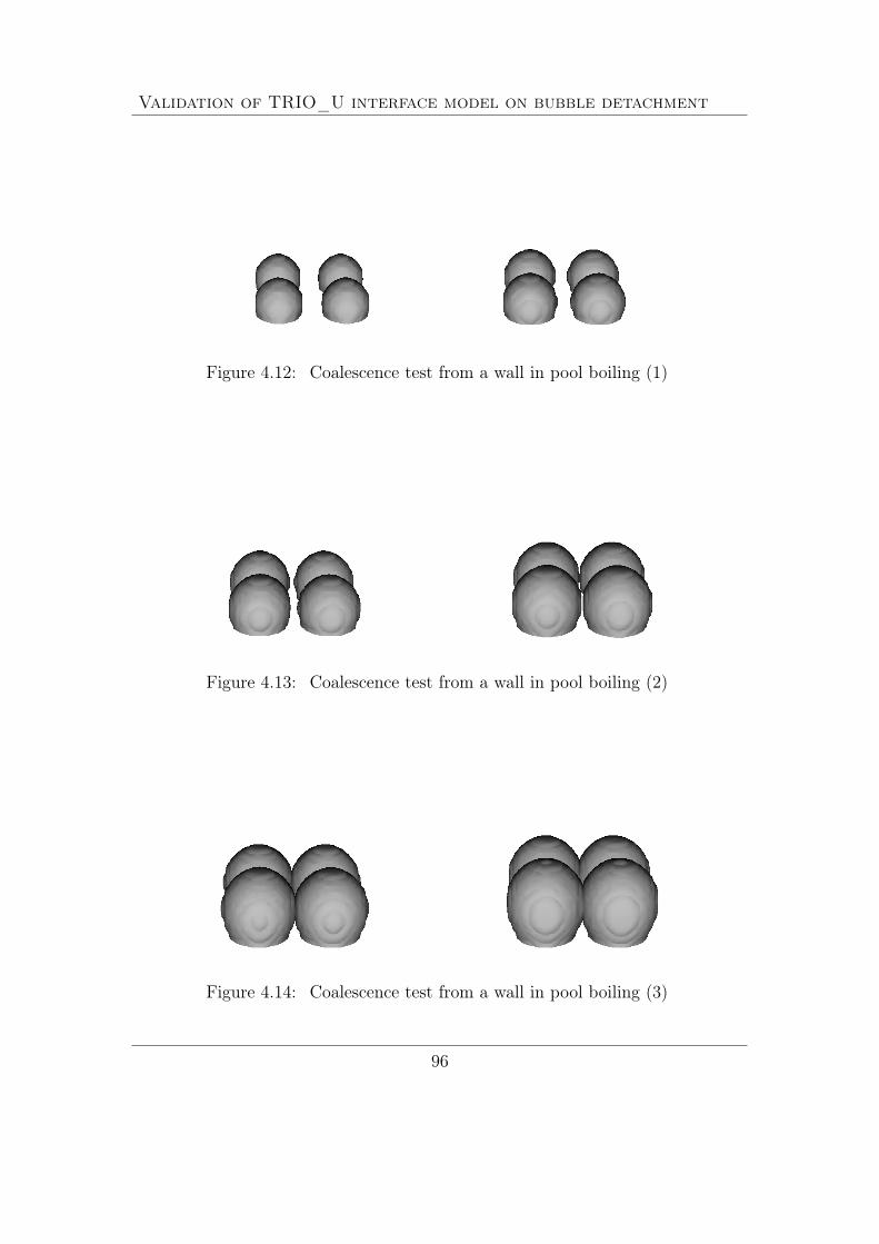
Validation of TRIO_U interface model on bubble detachment
Figure 4.12: Coalescence test from a wall in pool boiling (1)
Figure 4.13: Coalescence test from a wall in pool boiling (2)
Figure 4.14: Coalescence test from a wall in pool boiling (3)
96

Validation of TRIO_U interface model on bubble detachment
Figure 4.15: Simulation of bubble detachment from a wall in pool boiling (4)
Figure 4.16: Simulation of a bubble detachment from a wall in pool boiling (5)
Figure 4.17: Coalescence test from a wall in pool boiling (6)
97

Validation of TRIO_U interface model on bubble detachment
Figure 4.18: Coalescence test from a wall in pool boiling (7)
Figure 4.19: Coalescence test from a wall in pool boiling (8)
98

Validation of TRIO_U interface model on bubble detachment
4.2.4 Interface coalescence test
After simulating the behavior of a single bubble, we can study the growth andthe interaction between multiple bubbles within the same domain. The main goalof these simulations is to determine whether Trio_U can simulate in an accuratemanner the phenomenon of coalescence among different interfaces. Inside theconfiguration file you need to add a new instruction in order to introduce otherinterfaces within the domain, i.e. you need to add the desired number of bubbles.The fonction instruction followed by ajout_phase0 must be provided. Thesekeywords allow you to change the initial field that can be set by providing thefunctions in the coordinates (x, y, z) in the same way as for the single bubble case.For example, to obtain four bubbles the following code must be written as
conditions_initiales{fonction ((x-0.0015)^2+(y-0.0005)^2+(z-0.0002)^2-0.0003^2),fonction ajout_phase0((x-0.0005)^2+(y-0.0005)^2+(z-0.0002)^2-0.0003^2),fonction ajout_phase0((x-0.0005)^2+(y-0.0015)^2+(z-0.0002)^2-0.0003^2),fonction ajout_phase0((x-0.0015)^2+(y-0.0015)^2+(z-0.0002)^2-0.0003^2)}
In this way, four bubbles are created with center coordinates (0.0015, 0.0005, 0.0002),(0.005, 0.005, 0.0002), (0.0005, 0.0015, 0.002), (0.0015, 0.0015, 0.0002) and radius0.0003m. The physics of the problem is left unchanged compared to the studyof a single bubble. The four bubbles, subject to a constant heat flux, tend to growand interact with each other because of their very close positions. In order to seethe time evolution of these simulations we employ the VisIt software. Figures(4.12-4.19) show the rise and coalescence of these four bubbles. The bubbles tendto grow because of the heat flux from the lower wall, they coalesce and form asingle bubble. The resulting bubble detaches and begins its rise towards the topof the domain.
99

Bibliography
[1] A. Achilli et al., PERSEO Project: Experimental Facility Set-up and RE-LAP5 Code Calculations, Proc. 2nd EMSI and 40th European Two-PhaseFlow Group Meeting, Stockholm, Sweden, June 10-13, Royal Institute ofTechnology (KTH), Paper F3 (2002) 49
[2] F. Bassenghi, S. Bna, G. Bornia, A. Cervone, S. Manservisi and R. Scardovelli,Fissicu platform on cresco-enea grid for thermal-hydraulic nuclear engineer-ing, rapporto AdP ENEA-MSE CIRTEN , CERSE-UNIBO RL1302/2010(2010) 12, 15, 17, 19, 21, 22, 28, 31, 64, 70
[3] G. Bandini, C. Lombardo, P. Meloni and M. Polidori, Validation of catharev2.5 thermal-hydraulic code against full-scale perseo tests for decay heat re-moval in LWRs, Proceedings of the 18th International Conference on NuclearEngineering, ICONE18, Xi’an, China (2010) 56
[4] D. Bestion, G. Geffraye, The CATHARE code, CEA, Grenoble (F), Apr. 2002.37
[5] F. Bianchi et al., Thermal Valve System for LWR Applications, Proc. Post-SMIRT14 Seminar, Pisa, Italy (1997) 49
[6] F. Bianchi et al., Assessment of RELAP5 MOD3.3 and CATHARE 2 V1.5aagainst a Full Scale Test of PERSEO Device, Proc. 12th International Con-ference on Nuclear Engineering (ICONE12), Arlington, Virginia, USA (2004)58
[7] Y.A. Buyevich, B.W. Werbon, Dynamics of vapour bubbles in nucleate boiling,Int. J. Heat Mass Transfer 39 2409 (1996) 94
[8] CEA, CATHARE2 V2.5_1: User’s Manual, SSTH/LDAS/EM/2005-035,(2006) 37
[9] CEA, CATHARE2 V2.5_1: User’s Guidelines, DER-SSTH-LDAS-EM-2005-034, (2006) 40

BIBLIOGRAPHY
[10] CRESCO-ENEA GRID Project, http://www.cresco.enea.it. 7
[11] F. D’Auria, G.M. Galassi, F. Bianchi, P. Meloni, G. Cattadori, R. Ferri,SPES-99 IBLOCA Relap5/Mod3 pre-test and post-test analysis, CAMP 2000,Palermo (I) (2000) 44
[12] V.K. Dhir, Mechanicistic prediction of nucleate boiling heat transfer: achiev-able or a hopeless task ?, J Heat Transfer 128, 1 (2006). 94
[13] R. Ferri et al., PERSEO Project Experimental Data Report, SIET 01 014 RP02, Piacenza, Italy, (2002) 52
[14] R. Ferri, SPES-99 10: IB-LOCA in Cold Leg. Experimental data report, SIET00 777 RP 99, Piacenza; Nov. 26th, (1999) 36
[15] G. Geffraye et al., CATHARE 2 V2.5_2: a Single Version for VariousApplications, Proc. 13th International Topical Meeting on Nuclear ReactorThermal-Hydraulics (NURETH-13), Kanazawa, Japan (2009)
[16] HDF5 library: http://www.hdfgroup.org/HDF5/ 23
[17] G. Hazi, A. Markus, On the bubble departure diameter and release frequencybased on numerical simulation results, International Journal of Heat and MassTransfer 52, pp. 1472–1480 (2009) 94
[18] J. Kim, M.H. Kim, On the departure behaviors of bubble at nucleate poolboiling, Int. J. Multiphase Flow 32, 1269 (2006). 94
[19] R. F. Kulak and C. Fiala, NEPTUNE: A System of Finite Element Programsfor Three-Dimensional Nonlinear Analysis, Nuclear Engineering and Design,106, pp. 47-68 (1988) 17, 65
[20] R.F. Kulak and C Fiala, NEPTUNE: A system of finite element programs forthree-dimensional nonlinear analysis, Nuclear Engineering and Design, Vol.106 (1), pp.47-68 (1988) 17
[21] D. Bestion and A. Guelfi, Status and perspective of two-phase flow modellingin the NEPTUNE multi-scale thermal hydraulic platform for nuclear reactorsimulation, Nuclear Engineering and Technology, vol. 37 (6), (2005). 17
[22] J. Lavieville, E. Quemerais, S. Mimouni, and N. Mechitoua, NEPTUNE CFDV1.0 theory manual, EDF (2006) 17
101

BIBLIOGRAPHY
[23] Botjan Konar and Borut Mavko, Simulation of Boiling Flow ExperimentsClose to CHF with the NEPTUNE CFD Code, Hindawi Publishing Corpo-ration Science and Technology of Nuclear Installations, Article ID 732158, 8(2008) 17
[24] P. Meloni et al., Theoretical Design and Assessment of Isolation CondenserSystem Controlled with Thermal Valve, Proc. 6th International Conference onNuclear Engineering (ICONE6), San Diego, USA (1998) 49
[25] P. Meloni et al., Experimental Campaign and Numerical Analysis for the In-pool Energy Removal System for Emergency Operation, Proc. 13th Interna-tional Conference on Nuclear Engineering (ICONE13), Beijing, China, (2005)
[26] C. Medich, M. Rigamonti, M. Tarantini, SPES-2 the experimental test facilitysimulating the AP600 plant, Energia Nucleare, anno 13, gennaio-aprile (1996)37
[27] PARAVIEW visualization software: http://www.paraview.org. 31
[28] M. Rigamonti, SPES-2 Facility description, SIET 00 183 RI 92, Rev.1. Pia-cenza, 6-12-95 (1995). 36
[29] SATURNE CFD software, http://www.code-saturne.org. 20
[30] F. Archambeau, N. Mehitoua and M. Sakiz, Code SATURNE: A Finite Vol-ume Code for Turbulent flows, Int. J. Finite Volumes (2004) 20
[31] SALOME platform, http://www.salome-platform.org. 14, 26
[32] G. David, T.Chevalier and G. Meunier, Unification of Physical Data Models.Application in a Platform for Numerical Simulation: SALOME MagneticsIEEE Transactions, Volume: 43 (4), pp. 1661-1664 (2007) 14
[33] TRIO_U CFD software: http://www-trio-u.cea.fr. 18
[34] T. Hohnea, S. Kliema and U. Bieder, Modeling of a buoyancy-driven flowexperiment at the ROCOM test facility using the CFD codes CFX-5 andTRIO_U, Nuclear Engineering and Design Volume 236, Issue 12, pp. 1309-1325 (2006) 18, 85
[35] U. Biedera, and E. Graffardb, Benchmarking of CFD Codes for Applicationto Nuclear Reactor Safety Qualification of the CFD code TRIO_U for fullscale reactor applications, Nuclear Engineering and Design Volume 238, Issue3, pp 671-679 (2008) 18, 85
102

BIBLIOGRAPHY
[36] U. Biedera, G. Faucheta, S. Betinb, N. Kolevc, and D. Popovd, Simulationof mixing effects in a VVER-1000 reactor, Nuclear Engineering and DesignVolume 237, Issues 15-17, pp. 1718-1728 (2007) 18, 85
[37] USNRC, Three Mile Island Accident, Backgrounder, Office of Public Affair37
[38] VTK visualization software: http://www.vtk.org 29
[39] XDMF library: http://www.xdmf.org 24
[40] M. Zaccarelli, Sviluppo di un modello termo-fluidodinamico dell’impianto sper-imentale SPES-99 con il codice di sistema nucleare CATHARE-2, Thesis,University of Bologna (Italy), Engineering Faculty (2010) 39
103

List of Figures
1.1 SALOME graphical user interface . . . . . . . . . . . . . . . . . . . 131.2 Neptune graphical user interface. . . . . . . . . . . . . . . . . . . . 161.3 TRIO_U graphical user interface. . . . . . . . . . . . . . . . . . . . 181.4 SATURNE graphical user interface. . . . . . . . . . . . . . . . . . . 201.5 CATHARE graphical user interface (GUITHARE). . . . . . . . . . 221.6 HDF data viewer . . . . . . . . . . . . . . . . . . . . . . . . . . . . 231.7 XDMF data view . . . . . . . . . . . . . . . . . . . . . . . . . . . . 241.8 MED library . . . . . . . . . . . . . . . . . . . . . . . . . . . . . . . 261.9 SALOME Mesh generator . . . . . . . . . . . . . . . . . . . . . . . 271.10 GMSH mesh generator . . . . . . . . . . . . . . . . . . . . . . . . . 281.11 Basic interface for PARAVIEW . . . . . . . . . . . . . . . . . . . . 30
2.1 SPES-99 layout . . . . . . . . . . . . . . . . . . . . . . . . . . . . . 352.2 Vessel nodalization . . . . . . . . . . . . . . . . . . . . . . . . . . . 372.3 Loop A nodalization . . . . . . . . . . . . . . . . . . . . . . . . . . 382.4 PRZ, SG-A, SG-B pressure and core power . . . . . . . . . . . . . . 432.5 ACC-A/B flow rate and heater rod temperature . . . . . . . . . . . 442.6 Pressurizer pressure . . . . . . . . . . . . . . . . . . . . . . . . . . . 452.7 Accumulator A injection mass flow rate . . . . . . . . . . . . . . . . 462.8 Integral mass injected by the accumulators . . . . . . . . . . . . . . 462.9 Rod Clad Temperature in Lower Power Channel (left) and Lower/Middle
Power Channel (right) . . . . . . . . . . . . . . . . . . . . . . . . . 472.10 Rod Clad Temperature in Middle/Upper Power Channel (left) and
Upper Power Channel (right . . . . . . . . . . . . . . . . . . . . . . 47
3.1 The PERSEO (in-pool Energy Removal System for Emergency Op-eration) facility . . . . . . . . . . . . . . . . . . . . . . . . . . . . . 50
3.2 Test 9. Overall pool water level behavior (top) and HX pool relativepressure (bottom) . . . . . . . . . . . . . . . . . . . . . . . . . . . 53
3.3 Test 9. HX exchanged power (top) and overall pool temperatures(bottom) . . . . . . . . . . . . . . . . . . . . . . . . . . . . . . . . 54

LIST OF FIGURES
3.4 PERSEO facility steam duct and liquid line between the pools . . . 553.5 Injector or ending part of the steam duct in the overall pool . . . . 563.6 Coupling CATHARE-NEPTUNE . . . . . . . . . . . . . . . . . . . 573.7 Boundary conditions for the overall pool and injector components . 573.8 CATHARE discretization of the PERSEO test 9 . . . . . . . . . . . 583.9 HX pool water level behavior (left) and overall pool water level
(right) with CATHARE solution in pink. . . . . . . . . . . . . . . 593.10 HX pool relative pressure (left) and HX exchanged power (right)
with CATHARE solution in pink. . . . . . . . . . . . . . . . . . . 593.11 Overall pool temperatures (left) and HX tube wall temperature
(right) with CATHARE solution is pink. . . . . . . . . . . . . . . . 603.12 Steam Mass flow rate to OP pool . . . . . . . . . . . . . . . . . . . 613.13 Water Mass flow rate to HX pool (left) and water discharge Mass
flow rate (right) . . . . . . . . . . . . . . . . . . . . . . . . . . . . . 613.14 Directory of the NEPTUNE code . . . . . . . . . . . . . . . . . . . 623.15 Physical properties. . . . . . . . . . . . . . . . . . . . . . . . . . . . 653.16 Boundary conditions. . . . . . . . . . . . . . . . . . . . . . . . . . . 663.17 Overall pool temperature measurement positions. . . . . . . . . . . 673.18 Overall pool temperatures for different probes. . . . . . . . . . . . . 683.19 Chronology of the temperature main events for the probe TP6 . . . 703.20 Water mass flow rate to HX pool over the time interval [0 − 500]s
computed from CATHARE simulation. . . . . . . . . . . . . . . . . 723.21 Water discharge mass flow rate and steam mass flow rate to overall
pool over the time interval [0 − 500]s computed from CATHAREsimulation. . . . . . . . . . . . . . . . . . . . . . . . . . . . . . . . . 72
3.22 Water level at t = 150 s. . . . . . . . . . . . . . . . . . . . . . . . . 733.23 Water level at t = 204 s. . . . . . . . . . . . . . . . . . . . . . . . . 743.24 Computational and experimental temperature profiles in probes TP6
(1) and TP8 (2) as a function of time. . . . . . . . . . . . . . . . . 753.25 Steam mass flow rate to overall pool over the time interval [500 −
3000]s defined from CATHARE simulation . . . . . . . . . . . . . . 753.26 Water mass flow rate to HX pool and water discharge mass flow
rate over the time inteval [500 − 3000]s defined from CATHAREsimulation . . . . . . . . . . . . . . . . . . . . . . . . . . . . . . . . 76
3.27 Steam entering the injector (top) and injection of steam into water(bottom) . . . . . . . . . . . . . . . . . . . . . . . . . . . . . . . . . 77
3.28 Steam and water mixing (top) and inverse flow (bottom) . . . . . . 783.29 Temperature of the probes TP6 (red) and TP8 (green) from exper-
iment and NEPTUNE computation (blue and violet) and zoom ofthe temperature oscillations . . . . . . . . . . . . . . . . . . . . . . 79
105
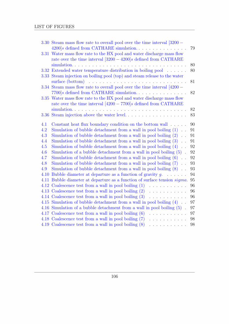
LIST OF FIGURES
3.30 Steam mass flow rate to overall pool over the time interval [3200−4200]s defined from CATHARE simulation. . . . . . . . . . . . . . . 79
3.31 Water mass flow rate to the HX pool and water discharge mass flowrate over the time interval [3200− 4200]s defined from CATHAREsimulation. . . . . . . . . . . . . . . . . . . . . . . . . . . . . . . . . 80
3.32 Extended water temperature distribution in boiling pool . . . . . . 803.33 Steam injection on boiling pool (top) and steam release to the water
surface (bottom) . . . . . . . . . . . . . . . . . . . . . . . . . . . . 813.34 Steam mass flow rate to overall pool over the time interval [4200−
7700]s defined from CATHARE simulation. . . . . . . . . . . . . . . 823.35 Water mass flow rate to the HX pool and water discharge mass flow
rate over the time interval [4200− 7700]s defined from CATHAREsimulation. . . . . . . . . . . . . . . . . . . . . . . . . . . . . . . . . 82
3.36 Steam injection above the water level. . . . . . . . . . . . . . . . . . 83
4.1 Constant heat flux boundary condition on the bottom wall . . . . . 904.2 Simulation of bubble detachment from a wall in pool boiling (1) . . 914.3 Simulation of bubble detachment from a wall in pool boiling (2) . . 914.4 Simulation of bubble detachment from a wall in pool boiling (3) . . 914.5 Simulation of bubble detachment from a wall in pool boiling (4) . . 924.6 Simulation of a bubble detachment from a wall in pool boiling (5) . 924.7 Simulation of bubble detachment from a wall in pool boiling (6) . . 924.8 Simulation of bubble detachment from a wall in pool boiling (7) . . 934.9 Simulation of bubble detachment from a wall in pool boiling (8) . . 934.10 Bubble diameter at departure as a function of gravity g. . . . . . . 944.11 Bubble diameter at departure as a function of surface tension sigma. 954.12 Coalescence test from a wall in pool boiling (1) . . . . . . . . . . . 964.13 Coalescence test from a wall in pool boiling (2) . . . . . . . . . . . 964.14 Coalescence test from a wall in pool boiling (3) . . . . . . . . . . . 964.15 Simulation of bubble detachment from a wall in pool boiling (4) . . 974.16 Simulation of a bubble detachment from a wall in pool boiling (5) . 974.17 Coalescence test from a wall in pool boiling (6) . . . . . . . . . . . 974.18 Coalescence test from a wall in pool boiling (7) . . . . . . . . . . . 984.19 Coalescence test from a wall in pool boiling (8) . . . . . . . . . . . 98
106

List of Tables
1.1 CRESCO front-end machines. . . . . . . . . . . . . . . . . . . . . . 81.2 Implementation status of the NURISP platform on CRESCO-ENEA
GRID . . . . . . . . . . . . . . . . . . . . . . . . . . . . . . . . . . 12
2.1 Main Characteristics of SPES-99 . . . . . . . . . . . . . . . . . . . 362.2 Steady state main parameters (1) . . . . . . . . . . . . . . . . . . . 392.3 Steady state main parameters (2) . . . . . . . . . . . . . . . . . . . 402.4 Main parameters of the reference steady state (1) . . . . . . . . . . 412.5 Main parameters of the reference steady state (2) . . . . . . . . . . 412.6 Test boundary conditions . . . . . . . . . . . . . . . . . . . . . . . . 422.7 Power curve . . . . . . . . . . . . . . . . . . . . . . . . . . . . . . . 45
3.1 The main PERSEO test parameters at full power operation duringthe transient phase of the test n.9 . . . . . . . . . . . . . . . . . . . 51
3.2 Chronology of main events characterizing test n.9 . . . . . . . . . . 523.3 Fluid and flow properties selected for PERSEO test 9 . . . . . . . . 643.4 Exact locations (in mm) of the probes for temperature measure-
ments with respect to the reference frame indicated in Figure 3.17. . 683.5 Chronology of the Temperature main events . . . . . . . . . . . . . 713.6 Initial conditions of OP and HX pool. . . . . . . . . . . . . . . . . . 71