risk and ambiguity in asset returns { cross-sectional di

Risk and Ambiguity in Asset Returns– Cross-Sectional Differences –

Chiaki Hara and Toshiki Honda

KIER, Kyoto University and ICS, Hitotsubashi University

KIER, Kyoto UniversityApril 6, 2017

Hara and Honda (Kyoto and Hitotsubashi) Risk and Ambiguity in Asset Returns April 6, 2017 1 / 32

Introduction

OutlineIntroduction

MotivationFF6 portfoliosReview of our results

ModelPreliminary results

“Reasonably” ambiguity-averse investorsBackgroundThe criterion we use

Risk-ambiguity decompositionRisk-ambiguity decompositionMinimal ambiguity partNumerical results

ConclusionSummary and future research


Introduction Motivation

Ambiguity in asset markets

I Explore implications of ambiguity and ambiguity aversion on portfoliochoices and asset returns (prices).

I Motivated to explain some phenomena that cannot be explained byexpected utility functions.

I Unlike those working on the equity premium puzzle, we do notaggregate stock returns in a single index such as S&P500.

I We concentrate on the composition of stocks in optimal portfolios.Cf. Chen and Epstein (2002) and Epstein and Miao (2003).


Introduction FF6 portfolios

Our “stocks”: FF6 portfolios

1. Sort out the stocks traded on NYSE, AMEX, and NASDAQ in termsof the market equity (market value, market capitalization) and theratio of the book equity (book value) to the market equity.

2. Partition them into six groups, according to whether the ME belongsto the top or bottom 50%, and whether the BE/ME belongs to thetop or bottom 30%, or neither.

3. Form the ME-weighted portfolio for each of the six groups:

Bottom 50% of ME Top 50% of ME

Bottom 30% of BE/ME SL BLMiddle 40% of BE/ME SN BN

Top 30% of BE/ME SH BH


Introduction FF6 portfolios

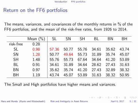
Return on the FF6 portfolios

The means, variances, and covariances of the monthly returns in % of theFF6 portfolios, and the mean of the risk-free rates, from 1926 to 2014.

Mean (%) SL SN SH BL BN BH

risk-free 0.28SL 0.98 57.36 50.77 55.76 34.61 35.62 43.74SN 1.28 50.77 49.64 55.73 31.89 35.74 45.07SH 1.48 55.76 55.73 67.64 34.64 41.20 53.89BL 0.91 34.61 31.89 34.64 28.62 27.43 31.63BN 0.97 35.62 35.74 41.20 27.43 32.89 38.32BH 1.19 43.74 45.07 53.89 31.63 38.32 50.95

The Small and High portfolios have higher means and variances.


Introduction Review of our results

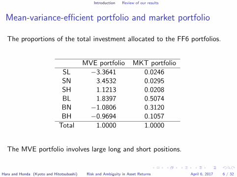
Mean-variance-efficient portfolio and market portfolio

The proportions of the total investment allocated to the FF6 portfolios.

MVE portfolio MKT portfolio

SL −3.3641 0.0246SN 3.4532 0.0295SH 1.1213 0.0208BL 1.8397 0.5074BN −1.0806 0.3120BH −0.9694 0.1057

Total 1.0000 1.0000

The MVE portfolio involves large long and short positions.



Introducing ambiguity to rationalize the market portfolio

I In the CARA-normal setting, the investor would hold a MVE portfolio.

I For what kind of utility functions is the MKT portfolio optimal?

I We use the ambiguity-averse utility functions of Klibanoff,Marinnacci, and Mukerji (2005).

I In particular, we extend the CARA-normal setting to the case wherethe expected asset returns are ambiguous but the covariance matrix isnot, and the second-order belief of expected asset returns is also amultivariate normal distribution.



Old results of ours

I Identified “basis portfolios,” which may constitute mutual funds.

I Proved that for every portfolio, there is an ambiguity-averse investorfor whom the portfolio is optimal if and only if the expected rate ofreturn of the portfolio exceeds the risk-free rate.

I For each such portfolio, identified a class of minimallyambiguity-averse investors for whom it is optimal.

I Proposed two notions of, and found, the least ambiguity-averseinvestor among them.



New results of ours

I Discuss why it is important to ask whether the observed choice isoptimal for a reasonably ambiguity-averse investor.

I Use a criterion to decide whether the investor for whom the observedchoice is optimal is reasonably ambiguity-averse, and argue that it isbetter than criteria that have been proposed in the literature.

I Investigate whether the representative investor is reasonablyambiguity-averse according to this criterion using the FF6 portfolios.


Model

OutlineIntroduction







Model Preliminary results

Ambiguity and ambiguity aversion

I Represent the returns of N assets by a random vector X.

I Denote the risk-free rate by R.

I Conditional on a random vector M , X has mean vector M :X|M ∼ N (M,ΣX|M ).

I Suppose that M ∼ N (µM ,ΣM ). It is the second-order belief.

I An ambiguity-averse utility function Uγ,θ is defined by

Uγ,θ

(a>X + bR

)= E

[uγ

(u−1θ

(E[uθ

(a>X + bR

)|M]))]

,

where uγ and uθ have CARA γ and θ. If γ > θ, then Uγ,θ isambiguity-averse.



Optimal portfolio

I The utility function Uγ,θ can be rewritten as

u−1γ (Uγ,θ(a

>X + bR)) = µ>Ma+Rb− θ

2a>ΣX|Ma−

γ

2a>ΣMa.

Cf. Maccheroni, Marinacci, and Ruffino (2013)

I The first-order condition for an optimal portfolio is

µM −R1 = (θΣX|M + γΣM )a = θ(ΣX + ηΣM )a

thus, a =1

θ(ΣX + ηΣM )−1(µM −R1), (1)

where η = γ/θ − 1 and ΣX = ΣX|M + ΣM .



Role of ambiguity in asset composition

I The optimal portfolio a is a scalar multiple of the MVE portfolio(1>Σ−1

X (µM −R1))−1Σ−1X (µM −R1) when ηΣM = 0.

I It is so even when ΣM = λΣX for some λ ∈ [0, 1]. Indeed, then,

a =1

θ(1 + λη)Σ−1X (µM −R1).

I It is so as long as ΣMa = λΣXa for some λ ∈ [0, 1].

I The expected excess return is always strictly positive:

a>(µM −R1) =1

θ(µM −R1)>(ΣX + ηΣM )−1(µM −R1) > 0.



The converse also holdsWe take ΣX as objective and observable, and ΣM as subjective andunobservable; and so is the decomposition ΣX = ΣX|M + ΣM .

Theorem 1. For every portfolio a ∈ RN , if a>(µM −R1) > 0, then thereis a (ΣM , η, θ) for which (1) holds.

I We have characterized the set of all such (ΣM , η, θ)’s by finding:

1. the supremum θ of the coefficients of risk aversion equal toa>(µM −R1)/(a>ΣXa); and

2. for each θ ∈ (0, θ), a unique (ΣθM , ηθ) that are smaller than any other

(ΣM , η) such that (ΣM , η, θ) belongs to the set.

I With the data of FF6 portfolios,

minθ∈(0,θ)

ηθ = 9.31.

Cf. ϕ(y) = (uγ ◦ u−1θ )(y) = −(−y)η+1.


“Reasonably” ambiguity-averse investors

OutlineIntroduction







“Reasonably” ambiguity-averse investors Background

Should we be fully content with these results?

I The condition of a strictly positive expected excess return seems weak.

I This implies that the predictive power of ambiguity-averse utilityfunctions also seems weak.

I Thus, we should ask whether a given portfolio can be optimal for a“reasonably” ambiguity-averse investor.

I How can we determine whether an investor is reasonablyambiguity-averse?



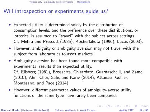
Will introspection or experiments guide us?

I Expected utility is determined solely by the distribution ofconsumption levels, and the preference over these distributions, orlotteries, is assumed to “travel” with the subject across settings.Cf. Mehra and Prescott (1985), Kocherlakota (1996), Lucas (2003).

I However, ambiguity or ambiguity aversion may not travel with thesubject from laboratories to asset markets.

I Ambiguity aversion has been found more compatible withexperimental results than expected utility.Cf. Ellsberg (1961), Bossaerts, Ghirardato, Guarnaschelli, and Zame(2010), Ahn, Choi, Gale, and Kariv (2014), Attanasi, Gollier,Montesano, and Pace (2014).

I However, different parameter values of ambiguity-averse utilityfunctions of the same type have rarely been compared.



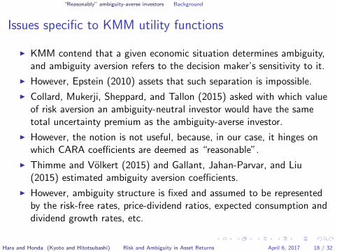
Issues specific to KMM utility functions

I KMM contend that a given economic situation determines ambiguity,and ambiguity aversion refers to the decision maker’s sensitivity to it.

I However, Epstein (2010) assets that such separation is impossible.

I Collard, Mukerji, Sheppard, and Tallon (2015) asked with which valueof risk aversion an ambiguity-neutral investor would have the sametotal uncertainty premium as the ambiguity-averse investor.

I However, the notion is not useful, because, in our case, it hinges onwhich CARA coefficients are deemed as “reasonable”.

I Thimme and Volkert (2015) and Gallant, Jahan-Parvar, and Liu(2015) estimated ambiguity aversion coefficients.

I However, ambiguity structure is fixed and assumed to be representedby the risk-free rates, price-dividend ratios, expected consumption anddividend growth rates, etc.


“Reasonably” ambiguity-averse investors The criterion we use

Our criterion of reasonable parameter values

I Let a be the MKT portfolio and choose a rationalizing (ΣM , η, θ).

I Then, we decompose the expected excess returns into two parts

µM −R1 = (Risk Part) + (Ambiguity Part)

Cf. Chen and Epstein (2002), Ui (2011), and Thimme and Volkert(2015).

I We (wish to) find a “minimal” ambiguity part by varying (ΣM , η, θ).


“Reasonably” ambiguity-averse investors The criterion we use

Why should we use this criterion?

I It depends only on the data of asset markets.

I It is valid even when ambiguity and ambiguity aversion cannot beseparated.

I It is consistent with an equilibrium comparative statics for a modelwith an ambiguity-averse representative investor.

I It admits a beta representation along the lines of the arbitrage pricingtheory of Ross and the multi-factor model of Fama.


Risk-ambiguity decomposition

OutlineIntroduction







Risk-ambiguity decomposition Risk-ambiguity decomposition

Basis portfolios

How does the optimal portfolio vary as η increases while ΣM is fixed?

Theorem 2. There are a positive integer K, K distinct elementsλ1, λ2, . . . , λK of [0, 1], and K portfolios v1, v2, . . . , vK such that:

1. ΣMvk = λkΣXvk for every k;

2. v>k ΣXv` = 0 whenever k 6= ` (the returns are independent); and

3. for every (θ, η), the optimal portfolio for the investor with thecoefficients θ and η of risk and ambiguity aversion coincides with

1

θ

K∑k=1

1

1 + λkηvk. (2)



Risk-ambiguity decomposition of expected excess returns

If η = 0, then the investor has a CARA expected utility function and hisoptimal portfolio coincides with

1

θΣ−1X (µM −R1).

Thus

1

θ

K∑k=1

vk =1

θΣ−1X (µM −R1), that is, µM −R1 =

K∑k=1

ΣXvk.

We decompose the expected excess returns into

K∑k=1

1− λk1 + λkη

ΣXvk +

K∑k=1

λk + λkη

1 + λkηΣXvk. (3)



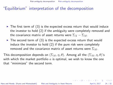
“Equilibrium” interpretation of the decomposition

I The first term of (3) is the expected excess return that would inducethe investor to hold (2) if the ambiguity were completely removed andthe covariance matrix of asset returns were ΣX − ΣM .

I The second term of (3) is the expected excess return that wouldinduce the investor to hold (2) if the pure risk were completelyremoved and the covariance matrix of asset returns were ΣM .

This decomposition depends on (ΣM , η, θ). Among all the (ΣM , η, θ)’swith which the market portfolio a is optimal, we wish to know the onethat “minimizes” the second term.


Risk-ambiguity decomposition Minimal ambiguity part

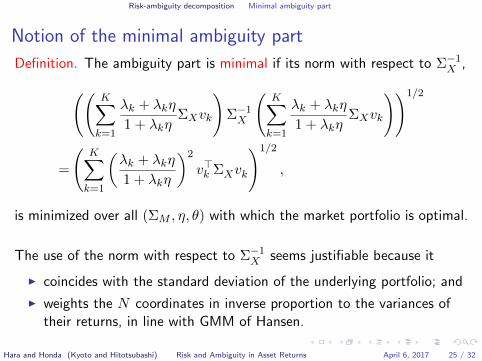
Notion of the minimal ambiguity part

Definition. The ambiguity part is minimal if its norm with respect to Σ−1X ,((

K∑k=1

λk + λkη

1 + λkηΣXvk

)Σ−1X

(K∑k=1

λk + λkη

1 + λkηΣXvk

))1/2

=

(K∑k=1

(λk + λkη

1 + λkη

)2

v>k ΣXvk

)1/2

,

is minimized over all (ΣM , η, θ) with which the market portfolio is optimal.

The use of the norm with respect to Σ−1X seems justifiable because it

I coincides with the standard deviation of the underlying portfolio; and

I weights the N coordinates in inverse proportion to the variances oftheir returns, in line with GMM of Hansen.



Our approach

I Instead of minimizing the ambiguity part over all (ΣM , η, θ)’s withwhich the market portfolio a is optimal, we minimize it only over all(Σθ

M , ηθ, θ)’s, defined after Theorem 1.

I For (ΣθM , η

θ), Theorem 2 holds with K = 2, λ1 = 0, and λ2 = 1.Moreover, (2) can be rewritten as

vθ1 +1

1 + ηθvθ2,

and, thus, the risk-ambiguity decomposition of asset returns is

µM −R1 = ΣXvθ1 + ΣXv

θ2

I Thus, our minimization problem is

infθ∈(0,θ)

((vθ2)>ΣXv

θ2

)1/2.



Solution of our minimization problem

Theorem 3.((vθ2)>ΣXv

θ2

)1/2is a strictly decreasing function of θ.

Moreover, ΣXvθ1 = θΣXa.

I The minimization problem is “solved” at θ = θ. Moreover, sincea>ΣXv

θ1 = a>(µM −R1), the expected excess return of the market

portfolio a can be explained completely by the risk part.

I It can be shown that((vθ2)>ΣXv

θ2

)1/2= Sharpe ratio︸︷︷︸

meanstandard deviation

of

(1

θΣ−1X (µM −R1)− a

)


Risk-ambiguity decomposition Numerical results

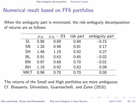
Numerical result based on FF6 portfolios

When the ambiguity part is minimized, the risk-ambiguity decompositionof returns are as follows:

µM µM −R1 risk part ambiguity part

SL 0.98 0.69 0.84 −0.15SN 1.28 0.98 0.81 0.17SH 1.48 1.19 0.92 0.27BL 0.91 0.63 0.65 −0.02BN 0.97 0.69 0.70 −0.01BH 1.19 0.92 0.83 0.09

MKT 0.98 0.70 0.70 0.00

The returns of the Small and High portfolios are more ambiguous.Cf. Bossaerts, Ghirardato, Guarnaschelli, and Zame (2010).



Another numerical result

When the coefficient of ambiguity aversion is minimized (ηθ = 9.31), therisk-ambiguity decomposition of returns are as follows:

µM µM −R1 risk part ambiguity part

SL 0.98 0.69 0.44 0.25SN 1.28 0.98 0.39 0.60SH 1.48 1.19 0.43 0.77BL 0.91 0.63 0.33 0.30BN 0.97 0.69 0.35 0.34BH 1.19 0.92 0.41 0.51

MKT 0.98 0.70 0.35 0.35

The High portfolios are more ambiguous, but the Small ones are not.



Issues on our approach

I As θ → θ, ηθ →∞.Thus, minimizing the ambiguity part of asset returns and minimizingthe coefficient of ambiguity aversion are very different.

I Yet, our approach is a hybrid of the two because we concentrate onthe (Σθ

M , ηθ, θ)’s.

I Collard, Mukerji, Sheppard, and Tallon (2015) found anambiguity-neutral investor who has the same certainty equivalents asthe calibrated investor to assess whether the latter is reasonablyambiguity-averse by using the former’s risk aversion.

I In our model, the ambiguity-neutral investor’s CARA is equal to θ forall rationalizing (Σ, η, θ)’s, but whether θ is reasonable is unknown.


Conclusion

OutlineIntroduction







Conclusion Summary and future research

Conclusion

I Extended the CARA-Normal setup to accommodate ambiguity.

I Established a necessary and sufficient condition for a given portfolioto be optimal for some ambiguity-averse investor.

I Discussed some criteria with respect to which the investor is“reasonably” ambiguity-averse.

I Assessed to what extent the representative investor isambiguity-averse based on the U.S. equity market data.

I Should spell out pros and cons of various criteria in view of“portability” and applications.

I Should separate the issue of ambiguity distribution across differentasset classes from that of reasonable ambiguity aversion.


risk and ambiguity in asset returns { cross-sectional di

Documents