risk evaluation on tunnel projects

i

TRITA-JOB PHD 1003 ISSN 1650-9501

Doctoral Thesis

MODEL FOR ESTIMATION OF TIME

AND COST BASED ON RISK EVALUATION

APPLIED ON TUNNEL PROJECTS

Therese Isaksson

Stockholm 2002

Division of Soil and Rock MechanicsRoyal Institute of Technology

Stockholm, Sweden

iii

This book is dedicated to my father Bengt H.S. (Lars)

“If I can throw a single ray of light

Across the darkened pathway to another;

If I can aid some soul to clearer sight

Of life and duty, and thus bless my brother;

If I can wipe from any human cheek a tear,

I shall not then have lived in vain while here”

remark by W.D. Gann, 1927 in “The Tunnel Thru the Air”

v

Preface

The research work presented in this thesis was carried out at the Division of Soil and Rock Mechanics, Royal Institute of Technology, Stockholm. The project is administrated by the Swedish Rock Engineering Research Foundation (SveBeFo) and financed by the Development Fund of the Swedish Construction Industry (SBUF), Skanska AB, the Swedish National Railroad Administration (Banverket) and the Swedish Rock Engineering Research Foundation.

Many people have in different ways contributed with information or assistance to this research work. It is not possible to mention all of you, and therefore I herewith express my gratitude for your support.

I will, however, specially thank:

Professor Håkan Stille, my supervisor. It has been rewarding to work under your committed supervision, and I am grateful for your support and for showing such a deep interest in the work.

My co-supervisor Dr Lars Olsson. Your continuous concern, support and suggestions have been very valuable for completion of this thesis.

The members of the reference group. I am very grateful to all of you for continuous support and encouragement. Your participation and comments have been most helpful, establishing balanced guidelines for this research. Your personal work and group discussions contributed to develop a better understanding on the subject.

The colleagues from my employments in Germany, Austria and Switzerland. I am profoundly grateful for your contribution with invaluable advice and information.

My colleagues and friends at the Division of Soil- and Rock Mechanics, Hydraulic Engineering and Center for Safety Research. Thank you not only for stimulating academic discussions but also for sharing part of your lives in moments of joy and struggle.

Finally I express my gratitude to my parents. Without your support and encouragement this thesis would not have been possible to make.

Stockholm, May 2002

Therese Isaksson

vii

Summary

The objective of this thesis is to improve the quality of the basis for making decisions about tender prices and budgets for tunnel projects by developing a model for the estimation of construction time and cost.

The planning and constructing of extensions to existing road and railway networks is an ongoing mission of transport infrastructure development. For functional, aesthetic or environmental reasons, a large number of these extensions are planned as tunnels. In the planning and procurement phases of tunnel projects, numerous decisions have to be made in relation to the tender price and project budget.

Literature studies shows that time schedules and costs for tunnelling projects are often exceeded. One reason for this is that pressure from various interests, including politicians, can often lead to adopting an inappropriate basis for making project decisions. Factors that mislead or underestimate time and cost estimations may sometimes be the only way of getting a project started. In order to reduce time and cost overruns, there are other demands placed on the basis for decision-making than those used in contemporary praxis.

Another reason for time and cost exceeding at tunnel projects is that they are sensitive to disturbances. The reason is that the tunnelling process is a “serial” type production system in two senses. Firstly, in a serial setting the possibility for changing workplace location—in this case a tunnel—is limited, except when more than one tunnel adit is made. Secondly, the possibility for executing more than one main work activity at a time is also limited in tunnelling projects. Therefore disturbances often have a larger impact on time and cost in tunnelling projects than in other types of construction.

In this study it has been stated that there are various risk factors with different impacts on cost and time values in tunnelling projects. It has therefore been concluded that it is important to make a clear distinction between normal cost and time and the undesirable events that cause

exceptional cost and time. Existing decision-aid estimation models, which handle variations in variables (such as the Successive methods and the Decision Aids in Tunnelling) do not consider normal time or cost and undesirable events separately in the estimations. Variation due to normal risk factors in this study is defined as “factors causing deviations in the normal time and cost span”. Examples of normal risk factors are performance-related factors like the advance rate of the tunnelling method. Undesirable events are defined as “events that cause major unplanned changes in the tunnelling process”. Undesirable events often occur due to physical factors like geological and hydrogeological conditions. Tunnel collapses, f looding and settlements are examples of undesirable events.

It has also been stated that there is a need for different basis for decisions depending on the responsibility of the part (client or contractor) in the project. The construction contracting method, as well as the stage of the project, affects which part that is responsible for the increases in cost and time that may occur due to different risk factors. Clearly, the client has the main responsibility for financing the project, however in some instances it may be appropriate for the contractor to pay for the cost of some of the risks. Variations in cost and time due to normal risk

viii

factors are often carried by the contractor, as normal risk factors fall mainly under the control of the contractor.

Estimations of project time and cost are normally made in a deterministic manner. There is however, a need to be able to handle variation in cost and time variables in the estimation. If the variables are stochastic, the total cost of a tunnelling method is expressed as a distribution curve, and the decision about which tunnelling method to use involves comparing their respective time- and cost distributions. Based on these decisions, the budget and tender price have to be determined by the client and contractor respectively. Analysis methods and decision criteria that take into consideration these distributions are required for selecting an appropriate tunnelling method. Commonly used decision-analysis methods and criteria are often applied for deciding between specific values. However there are other methods used for making decisions about tunnelling methods, tender prices and budgets. The main criteria used for decisions about which tunnelling method to use are not always the “minimum expected total cost and time”, but may also be for example, the probability of exceeding a certain value.

In order to respond to the demands placed on the basis for decision-making about tender price and budget, a new model for estimation has been developed. The model comprise five steps:

1. Determination of the geological and hydrogeological conditions along the alignment of the tunnel.

2. Division of the tunnel into geotechnical zones with “homogeneous” geological conditions and selection of a tunnelling method suited to the actual conditions.

3. Estimation of normal time and cost for each zone.

4. Estimation of exceptional time and cost for each zone.

5. Calculation of the total time and cost using Monte Carlo simulation.

The estimation model outlined in this thesis pays particular attention to the quantification of risks using different tunnelling methods. As each underground project is unique in purpose, requirements, location and surrounding environment, each project must therefore be subject to risk analysis specific to the given circumstances. In order to make the best choice of tunnelling method, the affect of adopting different degrees of robustness-increasing measures are assessed with respect to risk and production effort. The need for indicating the uncertainty of the results within the basis for decision-making is also emphasised in this study. The results can be used in different decision-making situations.

The estimation model described in this thesis has been applied to two case studies—the Grauholz Tunnel in Switzerland, and the South Marginal Zone of the Halland Ridge tunnel in Sweden. The application on these case studies shows that the results obtained from the estimation model are realistic, as the total construction time and cost obtained from the estimations roughly correspond to the actual construction time and cost.

ix

The separate estimation of normal and exceptional time and cost contribute to the clearness of the result. It has been shown that the normal time and cost impact mostly on the construction time and cost, and that estimation of the exceptional time and costs for each undesirable event identified is possible. This helps to increase the possibility for different parties (client and contractor) to use the results in various contractual and organisational situations.

Due to the distinctive estimation of different factors affecting the results, a sensitivity analysis can also be performed on the proposed estimation model, revealing which factors have the greatest effects on the results.

Application of the proposed estimation model also shows that the tunnelling method most suitable for the actual geological and hydrogeological conditions can be selected using the model. This is possible, as the normal and the exceptional costs that could be expected are shown in the results. Furthermore, the application also shows that it is important to consider different degrees of robustness in the tunnelling methods, as the time and cost of applying these measures often increase the normal cost, but reduce the normal time and the exceptional time and cost.

Finally, it is stated that this new estimation model has been developed for application on tunnelling projects, as the purpose with this thesis was to improve the quality of the basis for decision about bidprice and budget. However, it should be possible to find use for a modified version of the model within other fields, such as investment decisions while targeting operations involves risk factors such as future market trends and mass psychological behaviour within the financial markets.

xi

Zusammenfassung

Das Ziel der vorliegenden Arbeit ist die Entscheidungsgrundlage für Festlegung von Angebotpreisen und Budgets von Tunnelprojekten zu verbessern. Dies erfolgt durch die Entwicklung eines Modells zur Berechnung von Bauzeit und Projektskosten.

Planung und Ausbau der vorhandenen Strassen und Eisenbahnnetze sind die Aufgabe der Infrastrukturentwicklung. Aus funktionalen, ästhetischen wie auch Belangen der Umwelt wird eine immer gröβere Anzahl dieser Projekte als Tunnel ausgeführt. Bei der Planung und Vergabe von Tunnelprojekten muss eine Reihe von wichtigen Entscheidungen betreffend Angebotspreise und Projektdauer getroffen werden.

Aus der einschlägigen Literatur ist zu entnehmen, dass der Zeitplan und die Kosten für solche Projekte oft überschritten werden. Ein Grund dafür ist der Druck von verschiedenen Interessenten, einschließlich politische, die oft dazu führen, dass ungeeignete Grundlagen zur Entscheidungsfindung herangezogen werden. Unrichtige Bauzeit- und Kostenberechnungen können manchmal die einzige Möglichkeit sein um ein Projekt überhaupt anfangen zu können. Um Zeit- und Kostenüberschreitungen zu reduzieren gibt es jedoch andere Erfordernisse zu erfüllen, als die welche oft gängige Praxis ist.

Ein anderer Grund für Kosten- und Bauzeitüberschreitungen von Tunnelprojekte ist die Tatsache, dass diese Projekte besonderes störungsanfällig sind. Der Ursache dafür ist, dass das Tunnelbauprojekt ein serialer Prozess im zweifachen Sinne ist. Als erstes ist in einem serialen Ablauf, die Möglichkeit den Arbeitsplatz zu wechseln sehr begrenzt, außer es gibt mehrere Tunnelanschläge. Und zweitens ist die Möglichkeit mehr als eine Haupttätigkeit auszuführen ebenso begrenzt. Aus diesem Grund haben Störungen im Arbeitsablauf einen größeren Einfluss auf die Bauzeit und die Kosten eines Tunnelbauprojektes als bei anderen Bauvorhaben.

In dieser Studie wurde festgestellt, dass es verschiedene Risikofaktoren mit entsprechenden Auswirkungen auf Kosten und Bauzeit der Tunnelprojekte gibt. Daraus konnte gefolgert werden, dass eine klare Unterscheidung zwischen Normalkosten und Zeiten und unerwünschten

Ereignissen, die aussergewöhnlische Kosten und Zeit verursachen, erforderlich ist. Die bisherigen Berechnungsmodelle, mit denen es möglich ist Variationen in Eingabedaten anzugeben (sowie die Sucessive Methode und Decision Aids in Tunnelling) berücksichtigen nicht Normalkosten und Zeit getrennt von unerwünschten Ereignissen in der Kalkulation. Variationen auf Grund von normalen Risikofaktoren werden definiert als „Faktoren, die Veränderungen in der normalen Zeit und Kostenspanne verursachen“. Beispiele dafür sind leistungsbezogene Faktoren wie die Vortriebsgeschwindigkeit der jeweiligen Tunnelbaumethode. Unerwünschte Ereignisse aber werden definiert als „Ereignisse die gravierenden unvorhergesehenen Änderungen im Tunnelbauprozess verursachen“. Unerwünschte Ereignisse resultieren oft aus geologischen und hydrogeologischen Bedienungen. Tunnelverbrüche, Überschwemmungen und Setzungen sind Beispiele für unerwünschte Ereignisse.

Es wurde auch festgestellt, dass es einen Bedarf gibt, verschiedene Entscheidungsgrundlagen zu besitzen, je nach Verantwortung der Vertragsparteien (Bauherr oder Auftragnehmer) im Projekt. Die Methode der Vertragsgestaltung wie auch der Stand des Projektes beeinflussen

xii

welche der Parteien verantwortlich ist für die Kostensteigerung und Bauzeitverlängerung, die durch verschiedene Risikofaktoren verursacht werden kann. Der Bauherr trägt selbstverständlich die Hauptverantwortung für die Projektfinanzierung, aber in gewissen Fällen mag eine Verantwortung des Unternehmers für gewisse Kostenrisiken gerechtfertigt sein. Kosten und Bauzeitänderungen bedingt durch normale Risikofaktoren werden oft von Unternehmer getragen, da diese oft in seinen Verantwortungsbereich fallen.

Kostenberechnungen werden normalerweise auf deterministischem Weg festgelegt. Gleichwohl besteht jedoch ein Bedarf, Variable in den Eingabedaten einzuführen. Wenn die Eingabedaten stochastisch sind, werden die Gesamtkosten einer Tunnelbaumethode im Form einer Verteilungskurve ausgedrückt. Die Entscheidung welche Vortriebsmethode anzuwenden ist, erfolgt durch einen Vergleich der Kosten- und Zeitverteilungskurven. Auf Grund dieser Entscheidungen wird sowohl vom Bauherrn wie auch vom Unternehmer das Budget beziehungsweise der Angebotspreis festgelegt. Analysemethoden und Entscheidungskriterien, die Verteilungskurven berücksichtigen, werden zur Auswahl der am besten geeigneten Tunnelbaumethoden herangezogen. Allgemein übliche Entscheidungskriterien und Analysemethoden werden oft zur Entscheidung zwischen spezifischen Daten herangezogen. Es gibt aber andere Methoden zur Entscheidungsfindung für Tunnelvortriebsmethoden, Angebotspreise und Budgets. Die Hauptkriterien für eine Entscheidung, welche Vortriebsmethode zu wählen ist, sind nicht immer die erwarteten Mindestkosten und Zeit, sondern beispielsweise die Ûberschreitungswahrscheinlichkeit eines gewissen Wertes.

Um den Erfordernissen für die Entscheidung über Angebotspreis und Budget gerecht zu werden, wurde ein neues Modell zur Berechnung entwickelt. Das Modell umfasst fünf Stufen:

1. Festlegung der geologischen und hydrogeologischen Bedienungen entlang eine Tunnelstrecke.

2. Unterteilung des Tunnels nach „homogenen“ geologischen Verhältnissen und Auswahl möglicher Vortriebsmethoden.

3. Berechnung der Normalzeit und Kosten für jede Zone.

4. Berechnung der aussergewöhnliche Zeit und Kosten für jede Zone

5. Berechnung der Gesamtzeit und Kosten mit Hilfe der MonteCarlo Simulation.

Das dieser Arbeit zugrundeliegende Berechnungsmodell berücksichtigt in besonderer Weise eine Risikoabschätzung je nach studierter Vortriebsmethode. Da jedes einzelne Tunnelprojekt seine spezifische Zielsetzung, seine eigenen Rahmenbedienungen, seine spezifische Lage – und Umweltbedienungen hat, ist daher für jedes Projekt eine den gegebenen Umständen entsprechende Risikoanalyse durchzuführen. Um die beste Auswahl der zu verwendenden Tunnelbaumethode treffen zu können, wird der Einfluss verschiedener Stufen robustheitserhöhender Maßnahmen

xiii

festgelegt unter Berücksichtigung von Risiken und Leistungsänderungen. Die Unsicherheit, mit welchem die Ergebnisse in den Entscheidungsgrundlagen behaftet sind, wird in dieser Studie ebenfalls analysiert.

Das Berechnungsmodell, welches in der vorliegenden Arbeit erläutert wird, wurde bei zwei Fallstudien angewendet – dem Grauholztunnel in der Schweiz und dem Hallandstunnel in Schweden. Die Fallstudien zeigen, dass die Resultate des Berechnungsmodells realistisch sind, weil die Gesamtkosten und Bauzeit des Berechnungsmodells mit den tatsächlichen Kosten und Bauzeiten gut übereinstimmen.

Die getrennte Ermittlung von normalen und aussergewöhnlichen Kosten und Bauzeit trägt zur Klarheit des Ergebnisses bei. Es konnte gezeigt werden, dass meistens der Anteil der normalen Kosten und Bauzeit und der Anteil aussergewöhnlicher Kosten und Bauzeit für jedes unerwünschte Ereignis leicht zu identifizieren ist. Dadurch erhalten die Vertragspartner (Auftraggeber und Unternehmer) die Möglichkeit, die Ergebnisse in verschiedenen Vertrags- und organisatorischen Bedingungen entsprechend zu nützen.

Dank der getrennten Ermittlung der verschiedenen Faktoren, die die Ergebnisse beeinflussen, kann auch eine Sensibilitätsanalyse mit den vorgegebenen Berechnungsmodellen durchgeführt werden, um zu analysieren welche Faktoren am gravierendsten beeinflussen.

Mit dem vorliegenden Berechnungsmodell kann auch für die gegebenen geologischen und hydrogeologischen Bedienungen die am besten geeignete Vortriebsmethode ermittelt werden. Dies ist möglich, da die zu erwartenden normalen und aussergewöhnlichen Kosten und Bauzeit, in den Ergebnissen gezeigt werden. Weiteres hat die Applikation gezeigt, dass es wichtig ist verschiedene Stufen „Robustheitserhöhender Maßnahmen“ zu berücksichtigen, da diese Maßnahmen zwar meist die Normalkosten erhöhen, aber die aussergewöhnlichen Kosten und Bauzeiten reduzieren, und die Leistung insgesamt erhöhen.

Abschliessend ist hervorzuheben, dass dieses neue Berechnungsmodell für die Anwendung bei Tunnelprojekten entwickelt wurde, da es das Ziel dieser Arbeit war, die Grundlage für die Entscheidungsfindung bei Angebotspreisen und Projektbudgets zu verbessern. Es ist auch denkbar modifizierte Versionen des Berechnungsmodells in anderen Bereiche einzusetzen, wie zum Beispiel für Investitionsentscheidungen, weil Zielvorgaben Risikofaktoren beinhalten, wie zum Beispiel künftige Markttrends und massenpsychologisches Verhalten auf den Finanzmärkten.

xv

Sammanfattning

Syftet med denna avhandling är att förbättra kvaliteten på beslutsunderlag för anbudspris och budget för tunnelprojekt genom att utveckla en modell för beräkning av byggtid och byggkostnad.

Utbyggnad av infrastrukturen i form av väg- och järnvägsnät planeras och utförs i Sverige och Europa. På grund av funktionella, estetiska och miljömässiga skäl planeras en stor del av dessa utbyggnader som tunnlar. Vid planering och upphandling av tunnelprojekt måste en mängd beslut fattas, speciellt i samband med fastläggning av anbudspris och budget.

Erfarenheten visar, att många utförda tunnelprojekt inte genomförs inom planerad budget och tidsram. En orsak till detta är påtryckning från olika grupper, t.ex. politiker, vilket ofta leder till att oriktiga beslutsunderlag används. Att vilseleda eller underskatta tider och kostnader, är ibland det enda sättet att få ett projekt att påbörjas. För att reducera tids och kostnadsöverskridanden ställs andra krav på beslutsunderlag än de som i dag är praxis.

En annan orsak till tids och kostnadsöverskridanden hos tunnelprojekt är att de är känsliga för störningar. Detta beror på, att tunnelprocessen är ett seriellt produktionssystem i dubbel bemärkelse. Dels är möjligheten att ändra arbetsplats begränsad, förutom om det finns mer än en tunnelfront att arbeta vid. Dels är möjligheten att utföra mer än en huvudaktivitet samtidigt begränsad. Dessa båda faktorer bidrar till att störningar har en större inverkan på tider och kostnader för tunnelprojekt jämfört med andra typer av byggprojekt.

I denna studie har det konstaterats, att det finns olika typer av riskfaktorer, som påverkar tider och kostnader hos tunnelprojekt. En slutsats som dragits av detta är, att det är viktigt att göra en tydlig skillnad mellan normala riskfaktorer som orsakar normal variation hos tider och kostnader och oönskade händelser, som orsakar exceptionella tider och kostnader. Befintliga beräkningsmodeller, som behandlar variationer hos de ingående variablerna (såsom successiva metoden och DAT-metoden) beaktar inte normal tid och kostnad och exceptionella tider och kostnader separat i beräkningarna. Variation beroende på normala riskfaktorer definieras i denna studie som ”faktorer som orsakar avvikelse i det normala tid- och kostnadsspannet”. Exempel på normala riskfaktorer är faktorer relaterade till produktivitet, såsom framdriften hos drivingsmetoden. Oönskade händelser definieras som ”händelser som orsakar betydande oplanerade ändringar i drivningsprocessen”. Oönskade händelser orsakas ofta av fysiska faktorer, såsom geologiska och hydrogeologiska förhållanden. Exempel på oönskade händelser är ras, översvämning och sättningar.

Det har även konstaterats att det finns behov olika beslutsunderlag beroende på ansvarssituationen hos parterna i projektet (byggherre eller entreprenör). Den tillämpade kontraktsformen liksom i vilket stadium projektet befinner sig i påverkar vilken av parterna som har ansvar för ökningar av tider och kostnader som kan tänkas uppstå på grund av olika riskfaktorer. Givetvis har byggherren det övergripande ansvaret för finansiering av projektet, men även entreprenören kan ha ansvar för vissa kostnadsökningar. Speciellt tids och kostnadsökningar som orsakas av normala riskfaktorer, bärs vanligen av entreprenören, eftersom denne ofta kan kontrollera dessa faktorer.

xvi

Normalt utförs tid- och kostnadsberäkningar deterministiskt. Det finns dock behov av att hantera variationer i tids och kostnadsvariabler i beräkningarna. Om variablerna är stokastiska uttrycks de totala tiderna och kostnaden för en drivningsmetod som en fördelningskurva, och val av drivningsmetod kan ske genom att jämföra metodernas respektive fördelningar. Baserat på detta val kan budget och anbudspris bestämmas av byggherren respektive entreprenören. Analysmetoder och beslutskriterier, som tar hänsyn till fördelningar erfordras för att välja lämplig tunneldrivningsmetod. Vanliga beslutsanalysmetoder och kriterier är oftast till för beslut mellan specifika värden. Dock behövs andra metoder för beslut om tunneldrivningsmetod, anbudspris och budget. Kriterier, som kan används för beslut om tex vilken tunneldrivningsmetod, som skall användas behöver inte vara den lägsta förväntade totala kostnaden och tiden utan det är även viktigt att beakta faktorer som sannolikheten att överskrida en viss tid eller kostnad.

För att kunna motsvara de ställda kraven på beslutsunderlag för anbudspris och budget har en ny beräkningsmodell utarbetats. Modellen innehåller fem steg:

1. Bestämning av geologiska och hydrogeologiska förhållanden längs tunnelsträckan.

2. Uppdelning av tunneln i geotekniska zoner med homogena geologiska förhållanden och val av tunneldrivningsmetod, som kan användas i de aktuella förhållandena.

3. Beräkning av normal tid och kostnad för varje zon.

4. Beräkning av exceptionella tider och kostnader för varje zon.

5. Kalkylering av totala tider och kostnader med MontoCarlo simulering.

Beräkningsmodellen, som beskrivs i denna avhandling, lägger speciell vikt vid kvantifiering av risker hos olika tunneldrivningsmetoder. Eftersom varje undermarksprojekt är unikt gällande användningsområde, krav som skall uppfyllas och andra förutsättningar, måste en specifik riskanalys utföras för varje projekt. För att kunna välja den bästa drivningsmetoden beaktas även effekten av olika åtgärder för att höja robustheten. Dessa åtgärder påverkar såväl risker som produktiviteten. Vikten av att visa på osäkerheterna hos resultatet i beslutsunderlaget understryks även i denna studie. Resultatet av beräkning med modellen kan användas för att fatta olika beslut.

Beräkningsmodellen som beskrivs i denna avhandling har applicerats på två fallstudier – Grauholztunneln i Schweiz och Hallandsåstunneln (södra randzonen) i Sverige. Applikationen på dessa fallstudier visar, att resultatet som erhålls ur beräkningsmodellen är realistiska, då den totala byggtiden och kostnaden, som erhålls från beräkningen, motsvarar verklig byggtid och kostnad.

Den separata beräkningen av normal och exceptionell tid och kostnad bidrar till tydligheten hos resultatet. Det har visats, att den normala tiden och kostnaden påverkar byggtiden och kostnaden mest, och att beräkningen av exceptionella tider och kostnader för varje oönskad händelse, som identifierats, är möjlig. Detta bidrar till att öka möjligheten för varje part (byggherre och entreprenör) att använda resultatet i olika kontrakts-och entreprenadformer.

xvii

Genom att olika faktorer, som påverkar resultatet beräknas separat, kan en känslighetsanalys också utföras med den föreslagna beräkningsmodellen. De faktorer, som har störst inverkan på resultatet, kan härmed identifieras.

Applikation av den föreslagna beräkningsmodellen visar också, att den drivningsmetod, som är mest lämpad för de aktuella geologiska och hydrogeologiska förhållandena, kan väljas. Detta är möjligt, då de normala och exceptionella tider och kostnader, som kan förväntas, visas i resultatet. Vidare visar applikationen vikten av att betrakta olika grader av robusthet hos drivningsmetoden, då tider och kostnader för dessa åtgärder ofta ökar den normala kostnaden men minskar den normala tiden och den exceptionella tiden och kostnaden.

Slutligen kan det konstateras, att den nya beräkningsmodellen har utvecklats för att appliceras på tunnelprojekt, då syftet med denna avhandling var att förbättra kvaliteten hos beslutsunderlag för tex anbudspris och budget. Det borde dock vara möjligt att kunna använda en modifierad version av modellen inom andra områden, såsom investeringsbeslut, då inriktning av verksamheten innehåller riskfaktorer såsom kommande marknadstrender och masspsykologiska beteendemönster på den finansiella marknaden.

xix

Table of Contents

PREFACE ....................................................................................................... V

SUMMARY ...................................................................................................VII

ZUSAMMENFASSUNG ..................................................................................XI

SAMMANFATTNING.....................................................................................XV

TABLE OF CONTENTS ................................................................................XIX

NOTATIONS AND SYMBOLS .................................................................... XXIII

1 INTRODUCTION...................................................................................... 1

1.1 Background .............................................................................................................. 1

1.2 Scope of work .......................................................................................................... 2

2 DEMANDS ON ESTIMATION MODELS FOR TUNNEL PROJECTS.............. 5

2.1 Introduction.............................................................................................................. 5

2.2 Risks in tunnel projects ........................................................................................... 9

2.2.1 Introduction ............................................................................................................................. 9

2.2.2 Characteristics of tunnel projects ..................................................................................... 9

2.2.3 Risk factors in the tunnelling process .............................................................................11

2.2.4 Conclusion ............................................................................................................................. 20

2.3 Calculation methods for handling variations in cost and time due to risks .............21

2.3.1 Introduction ............................................................................................................................21

2.3.2 Methods used to calculate variation in cost and time due to normal risk factors ...... 22

2.3.3 Methods to calculate extra ordinary cost and time .................................................... 27

2.3.4 Contemporary Decision-support estimation models.................................................. 30

2.3.5 Conclusions ........................................................................................................................... 35

2.4 Decision making......................................................................................................36

2.4.1 Introduction ........................................................................................................................... 36

2.4.2 Factors affecting decisions ................................................................................................ 37

2.4.3 Decision-analysis methods and criteria ......................................................................... 45

2.4.4 Conclusion ............................................................................................................................. 49

2.5 Conclusions regarding the demands on estimation models ....................................50

xx

3 CHARACTERISTICS OF TUNNELLING METHODS AFFECTING TIME AND

COST ESTIMATION ............................................................................... 53

3.1 Introduction............................................................................................................ 53

3.2 General aspects affecting the range of viability of various tunnelling methods ..... 54

3.2.1 General factors .....................................................................................................................54

3.2.2 Examples using different tunnelling methods ..............................................................56

3.2.3 Conclusion ............................................................................................................................. 67

3.3 Geotechnical characteristics affecting the advance rate of tunnelling methods ..... 68

3.3.1 Introduction ...........................................................................................................................68

3.3.2 Examples using different tunnelling methods ..............................................................68

3.3.3 Conclusion ............................................................................................................................. 76

3.4 Undesirable events affecting tunnelling methods................................................... 77

3.4.1 Introduction ........................................................................................................................... 77

3.4.2 Examples from different tunnelling methods ...............................................................79

3.4.3 Conclusions ...........................................................................................................................95

3.5 Measures for increasing robustness....................................................................... 95

3.5.1 Robustness and the tunnelling method .........................................................................95

3.5.2 Examples from different tunnelling methods ............................................................... 97

3.5.3 Concluding comments on increasing robustness ..................................................... 103

3.6 Conclusions ...........................................................................................................103

4 MODELLING OF TIME AND COST........................................................105

4.1 Introduction...........................................................................................................105

4.2 A theoretical estimation model .............................................................................105

4.2.1 Expressing parameters..................................................................................................... 105

4.2.2 Normal time and cost....................................................................................................... 106

4.2.3 Exceptional time and cost ............................................................................................... 110

4.2.4 Concluding comments on the theoretical model....................................................... 110

4.3 Practical modelling ............................................................................................... 111

4.3.1 Introduction to practical modelling ...............................................................................111

4.3.2 Geotechnical modelling .....................................................................................................111

4.3.3 Modelling of normal variation of cost and time.........................................................113

4.3.4 Modelling undesirable events ......................................................................................... 122

4.4 Conclusions ...........................................................................................................129

5 CASE STUDY – THE GRAUHOLZ TUNNEL............................................137

5.1 Introduction...........................................................................................................137

5.1.1 About the chapter .............................................................................................................. 137

5.1.2 Description of the project ............................................................................................... 137

5.1.3 Geology and hydrogeology .............................................................................................. 138

5.1.4 Tunnelling methods and corresponding robustness-increasing measures......... 142

xxi

5.2 Estimation of time and costs................................................................................. 142

5.2.1 Normal time and costs......................................................................................................142

5.2.2 Exceptional time and cost ................................................................................................154

5.2.3 Total time and cost .............................................................................................................160

5.3 Comparison of estimated and actual time and costs ............................................ 165

5.3.1 Introduction to the section ...............................................................................................165

5.3.2 Exceptional time and cost ................................................................................................166

5.3.3 Total construction time and cost ....................................................................................170

5.4 Factors affecting the result of the Estimation of time and cost for combined shield ... 173

5.4.1 Degree of correlation.........................................................................................................173

5.4.2 Type of costs considered .................................................................................................. 174

5.5 Factors affecting decision making ......................................................................... 175

5.5.1 Contract and organisation ................................................................................................175

5.5.2 Degree of robustness ........................................................................................................176

5.6 Conclusion............................................................................................................. 177

6 CASE STUDY: THE SOUTH MARGINAL ZONE OF THE HALLAND RIDGE

TUNNEL PROJECT.............................................................................. 179

6.1 Introduction........................................................................................................... 179

6.1.1 About the chapter ...............................................................................................................179

6.1.2 Description of the project ................................................................................................179

6.1.3 Geology and hydrogeology ...............................................................................................180

6.1.4 Tunnelling methods ............................................................................................................182

6.2 Estimation of time................................................................................................. 183

6.2.1 Normal time .........................................................................................................................183

6.2.2 Exceptional time..................................................................................................................188

6.2.3 Total construction time .....................................................................................................191

6.3 Comparison of estimations with the actual results ............................................... 193

6.3.1 Introduction to the section ...............................................................................................193

6.3.2 Normal time .........................................................................................................................196

6.3.3 Exceptional time..................................................................................................................196

6.3.4 Total construction time .....................................................................................................198

6.4 Factors affecting the results .................................................................................. 199

6.4.1 Degree of correlation.........................................................................................................199

6.4.2 Type of time considered ...................................................................................................199

6.5 Factors affecting decision making .........................................................................200

6.5.1 Contract and project organisation................................................................................. 200

6.5.2 Robustness ...........................................................................................................................201

6.6 Conclusion.............................................................................................................202

xxii

7 SUMMARY AND CONCLUSION ............................................................ 203

7.1 Introduction.......................................................................................................... 203

7.1.1 Demands on estimation models for tunnel projects ................................................ 203

7.1.2 Characteristics of tunnelling methods affecting the estimation of time and cost ..205

7.2 Theoretical estimation model................................................................................205

7.3 Conclusion from application of the estimation model ...........................................207

8 PROPOSALS FOR FURTHER RESEARCH ............................................. 209

REFERENCES ............................................................................................ 213

APPENDIX: DETAILS OF THE ESTIMATION – GRAUHOLZ AND

HALLANDSRIDGE TUNNEL...........................................................................III

xxiii

Notations and symbols

Roman letters

A Rock quality

B Clay content

C Water leakage

Ce

Exceptional cost

Cek

Exceptional cost for the undesirable event “k”

Ci

Cost of a zone

Cik

Consequence of undesirable event “k”

Cn

Normal cost

CNf

Fix normal cost

CNi

Normal cost in zone i

CNq

Quantity-dependent normal cost

CNt

Time-dependent normal cost

Ctot

Total cost

d1

Distance between mean crossings

E(y) Expectation of production effort

g(x(l)) Production effort

i Event type

j Cost type

k Event number

L Tunnel length

mi

Mean value

mQ

Mean value of the production effort

mz

Mean value of the cost variable

p Probability for undesirable event

P´´[θi] Posterior probability of θ

i given the information z

k

P[zk θ

i] Probability of getting information z

k given the outcome θ

i (likelihood)

P´[zk θ

i] Prior probability of θ

i

Qf

Production effort related to the fix cost

Qq

Production effort related to quantity

Qt

Time related production effort

T Working time

t Time

x(l) Geotechnical characteristic

y Production effort

z Cost variable

zf

Cost variable for the fix cost

zq

Quantity dependent cost variable

zt

Time dependent cost variable

xxiv

Greek letters

Γg

Reduction factor

δl

Scale of f luctuation

θi

Statistical parameter I

θj

Statistical parameter jλ Failure frequencyη Repair rate

σi

Standard deviation (production effort)

σQ

Standard deviation of the production effort

σy

Standard deviation at a point

σz

Standard deviation of the cost variable

Abbreviations

AEA Action Error Analysis

PERT Program Evaluation and Review Technique

PROF Prediction of Operator Failure rate

PSF Performance Sharping Factors

SLIM Success Likelihood Index Method

SMZ South Marginal Zone

TBM Tunnel Boring Machine

THERP Technique for Human Error Rate Prediction

1

1 Introduction

1.1 Background

The planning and constructing of extensions to existing road and railway networks is an ongoing component of transport infrastructure development. For functional, aesthetic or environmental reasons, a large number of these extensions are planned as tunnels. In the planning and procurement phases of tunnel projects, numerous decisions have to be made in relation to the tender price and project budget. Selecting the most appropriate tunnelling method is also one of the most important decisions to be made in the planning stage. Selection often involves choosing between fully-mechanised or ‘conventional’ tunnelling methods. When fully-mechanised tunnelling methods are chosen, the one tunnelling machine must be able to handle the whole range of possible uncertainties in the geological conditions it is expected to encounter. Furthermore, these machines do not have direct access to the face, making this task more complicated. Therefore, full-face machines (such as TBMs) and fully-enclosed shield machines face increased risks where complex geological conditions are encountered. The ability to select the most appropriate tunnelling method places great demands upon the client and the engineer.

It is therefore important to establish a sound basis for making these decisions. Estimating total construction time and total construction cost forms the basis for many decisions. Literature studies show that times and costs are often exceeded. One reason for this is that pressure from various interests, including politicians, can often lead to adopting an inappropriate basis for making project decisions. Factors that mislead or underestimate time and cost estimations may sometimes be the only way of getting a project started (Kastbjerg, 1994). A study by Pickrell, looking at US Rail Transit projects from 1971-1987, shows that cost overruns can arise when the structure of the estimation model used is incorrect—that is where models are incorrectly applied or the numerical outputs of these are misinterpreted (Kastbjerg, 1994). In order to reduce time and cost overruns, there are other demands placed on the basis for decision-making than those used in contemporary praxis.

The objective of this thesis is to improve the quality of the basis for making decisions about tender price and budgets for tunnel projects by developing a model for the estimation of construction time and cost. The estimation model outlined in this thesis pays particular attention to the quantification of risks using different tunnelling methods. In order to make the best choice of tunnelling method, the affect of adopting different degrees of robustness-increasing measures in the tunnelling method is assessed with respect to risk and production effort. The results can therefore be used in different decision-making situations. As each underground project is unique in purpose, requirements, location and surrounding environment, each project must therefore be subject to risk analysis specific to the given circumstances. The need for indicating the uncertainty of the results within the basis for decision-making is also emphasised in this study.

2

1.2 Scope of work

This thesis deals with the issue of estimating time and cost, and presents a model for analysing and quantifying risks in order to obtain a sound basis for decision-making in tunnel projects. Estimating basic costs alone does not provide an adequate basis for this sort of decision-making, however using a model that incorporates the impact of different geological factors into the estimation of risks and production effort might. Just such an estimation model has been developed and described in this thesis, having the same purpose as the Decision Aids in Tunnelling (DAT) simulation programme developed at Massachusetts Institute of Technology (MIT) (Einstein & Vick, 1974; Einstein et al., 1991; Salazar, 1983), but which considers risk explicitly.

The thesis has been structured parts as follows. The demands placed on an estimation model and the characteristics of tunnelling methods that affect the estimation are described at the beginning. Further into the thesis the estimation model is described in detail, and finally the estimation model is applied to two case studies.

More specifically, following the introduction to the thesis in Chapter 1, Chapter 2 describes the demands that ought to be placed on an estimation model for tunnel projects. This description starts with the factors that characterise tunnel projects and risk factors that may impact on the tunnelling process. Contemporary calculation methods used to handle variations in cost and time due to various risk factors, and contemporary decision-aid-estimation models, principles and limitations are then explained and discussed. The chapter goes on to present factors affecting decision-making, decision-analysis methods and decision criteria. The material in this chapter is based to a large extent on literature survey.

Chapter 3 deals with characteristics of tunnelling methods that affect the estimation of time and cost. This chapter starts with general aspects on the geological range of viability of tunnelling methods. Based on literature studies, the chapter then presents geotechnical characteristics that affect the production effort, undesirable events that affect the total cost and time, and the importance of applying robustness-increasing measures. Examples from various tunnelling methods (tunnelling machines and conventional methods) are provided for all the factors presented. In a report by Isaksson (1996) have parts of the material earlier been presented.

Chapter 4 describes the theoretical estimation model. The modelling of geotechnical characteristics, normal variation in time and cost, and exceptional time and cost in the model are all described. The chapter concludes by summarising the model into five working steps. Parts of the material have earlier been presented. by Isaksson et al (1999a,b).

In Chapter 5, the estimation model is applied to the first case study, the Grauholz Tunnel Project in Switzerland. The excavation method used in this project and investigated here, utilises tunnelling machines. The five working steps in the estimation model developed in the thesis have then been followed for the estimation of total construction time and cost in the project. As this tunnel project was completed some years ago, comparisons between the estimated and actual time and cost can therefore be discussed. Factors affecting the results of the estimations

3

and the tunnelling decisions that were made are also discussed. In a licentiate thesis by Isaksson (1998b) and in Isaksson (1998a) have parts of the material earlier been presented.

In Chapter 6, the estimation model has been applied to second case study, the Halland Ridge Tunnel Project in Sweden. The excavation method used in this project and investigated here, is referred to as a conventional method. The five working steps described in Chapter 4, dealing with the estimation of construction time, have been followed through in relation to this case study. Only a specific section of the Halland Ridge Tunnel Project, which was completed some years ago (the South Marginal Zone) was studied here, enabling comparisons between the estimated and actual construction time to be made and discussed. Factors affecting the results of the estimations and the decision-making process have also been presented.

Finally, general conclusions are presented in Chapter 7, and guidelines for further research in Chapter 8.

5

2 Demands on estimation models for tunnel projects

2.1 Introduction

Knowledge relating to costs and time for construction projects normally serves as the basis on which important decisions are made. In order to obtain cost and time information for a project, certain estimations have to be made. The aim of this chapter is to point out the requirements facing a system for the estimation of cost and time for tunnel projects, which takes risks into consideration.

As with all construction projects, tunnel projects are affected by disturbances. The tunnelling process can be seen as a cyclical process, where the main activities are executed in series (Salazar 1985). Disturbances often have larger impacts on cost and time in series projects such as tunnel projects than in other project types. Disturbances are often caused by factors like the prevailing geological, technological (equipment and machinery) and economic conditions. These factors are often correlated, and may lead to increases in actual costs and times compared with those expected.

Figure 2.1 illustrates the impact of the higher levels of uncertainty that exist in tunnelling compared with other types of construction. This figure shows that surface-built projects with relatively simple production process, such as pipeline projects, have less variability in their range of tenders than the more complex underground tunnelling projects. The spread between the mean tender value and the engineer’s cost estimate is also larger in tunnel projects.

Figure 2.1. Tender data for four types of heavy-construction projects (Swedish Bureau of

Reclamation Projects, 1965-70). Histograms showing the number of tenders vs. percentage

difference from the engineer’s estimate (Moavenzadeh & Markow, 1976).

Knowledge about the commonality and magnitude of cost and time overruns in tunnel projects can be obtained by studying various infrastructure projects (including tunnels), as done for

6

example by Kastbjerg (1994), Andreossi (1998), Nylén (1999) and HSE (1996). The studies referred to below illustrate cost overruns for various infrastructure projects. The exact basis and framework of each study will not be analysed here in this thesis.

A study of 180 projects around the world in the 1960s, undertaken by Merewitz shows that cost overruns of about 50% were relatively common (see Kastbjerg, 1994). It was also concluded that cost overruns tended to increase in rapid-transit projects using state-of-the-art technology, compared to ongoing construction and renovation programmes. Larger projects were also subject to higher cost-overruns than smaller projects. Common reasons for these overruns were inflation and unforeseen changes in scope occurring after the authorisation of the project.

In a study of 41 infrastructure projects (involving tunnels and bridges) carried out by Kastbjerg in 1994, it was found that the majority of the projects had cost overruns of over 50%. In 32% of the projects the cost overruns ranged from 50 to 100% (see Figure 2.2). Kastbjerg also found that some construction projects in developing countries had cost overruns of up to 500%.

Figure 2.2 Construction cost overruns in 41 infrastructure projects, after Kastbjerg (1994).

The reasons behind the differences between estimated and actual construction costs of 15 Swedish construction projects have also been studied by Kastbjerg (1994). The total estimated value of these projects from the Swedish Road Directorate and the Swedish National Rail Administration was SEK 9.8 billion. The average cost overrun was 33% (see Figure 2.3). Underestimation was more common at the Swedish National Road Administration, where the construction cost increased by an average of 86% from the original cost estimates. The average increase in the Swedish National Rail Administration was 17%.

Figure 2.3 Construction cost overruns in 15 Swedish construction projects, after Kastbjerg (1994).

7

From the above study it can be concluded that construction costs are often underestimated and that cost estimates rise as projects proceed. The earlier an estimate is made the larger the potential cost increase.

Worldwide data including HSE (1996), show that the collapse of tunnels, especially those built in soft ground in urban areas, can result in major consequences for those working in the tunnels, members of the public, the overall infrastructure, and the surroundings. There are indications that for every major event such as a collapse, there are likely to be many more minor and associated incidents. There is however, very little information in the literature about these sorts of events. One study however, shows that the ratio of events causing injury to personnel, to non-injury events is 1:14 (HSE, 1993). Waninger (1982) reports on the investigation into 32 collapses in Germany between 1976 and 1982. Two of these involved fatal accidents, 12 involved unspecified injuries, and 20 caused no injuries to personnel (HSE, 1996).

The cost of substandard quality (quality failure) in major civil engineering projects has been studied by Nylén (1999). In the latter phases of civil works some 503 failures were registered. Altogether these failures cost some SEK 9.1 million, which corresponds to approximately 8% of the total construction cost. From the study it was concluded that just a few complex failures accounted for the major part of the failure cost—10% of the failures accounted for 90% of the failure cost. Most of the failures were caused in one stage of the process, but led to consequences in another. Some 80% of the failure cost incurred during the construction phase was not caused during the construction process. Furthermore it was concluded that more than 60% of the failure costs over SEK 30,000 was due to inflicted uncertainty (uncertainty inflicted by the refusal to learn from previous projects) and can thus be remedied. According to Nylén (1999), 34% of the failure cost can be reduced if the uncertainty causing the failure could be transformed into a calculable risk. Only 5% of the failure cost was found to be irreducible, that is 95% of the failure cost is the result of poor information feedback from previous projects. Incomplete soil investigations or failed interpretations of these were the reasons behind 34% of the total failure cost (Nylén, 1996).

A study by a Swiss insurance company (Andreossi, 1998) showed that 50-60% of all the declared losses were below US $1.5 million and represented 40-70% of the total claim costs. For power plants and roadworks, 90-100% of all declared losses were below US $7 million and represented 85-100% of the total claim costs. This was also valid for underground railways, when major ”extraordinary” losses and high-frequency losses were excluded. When the extraordinary losses are included, about 800 individual losses (90% of these relating to third-part liability) within one project amounted to more than US $50 million, and one single accident in another project came to US $230 million, and which represented about 90% of the insured value of the entire project. It was concluded from the study that one huge loss or several medium losses resulted in damages totalling nearly 100% of the project cost. The reasons for these cost and time overruns can often be related to human factors. Misunderstanding the concept and construction methods and so-called ”critical items” often contribute to the overruns.

The above-mentioned studies show that major increases in cost and time compared with the expected figures occur often. This indicates that there may be shortcomings in the estimation

8

methods used today. A short description of a commonly-used method follows.

Estimation of budget and tender prices for construction projects are done deterministically. The principle of deterministic estimation of construction cost and time budgets has been discussed in the literature (Quellmelz, 1987; Platz, 1991). Depending on the stage in the construction process and the information available, different types of deterministic estimations can be made, including for example functional estimation, product estimation or production estimation (Danielson, 1975). Functional estimation uses only information about how the construction object is going to be used, as only the purpose of the construction is provided. Product estimation is based on the technical design data for the construction object. Unit costs for the different parts of the construction, or costs per unit of the products, materials and work are used as the basis for product estimation. Production estimation is based on the construction activities for a given construction method and final technical solution. This method provides the greatest accuracy and is common practice today when estimating tender price and detailed budgets (Danielson, 1975).

There are many different cost types to consider in production estimation. These cost types can be basic costs, on costs and overhead costs (Drees & Bahner, 1992; Bunner et al.,1981). Basic costs include: wages and other remunerations, costs for construction materials including transportation and material losses, plant costs including plant operators, hiring, repairs, spare parts, cabling, tyres, fuel, freight and charges (harbours and other authorities), clothing, and sales tax. On costs are those that are indirectly rather than directly needed in construction. These consist of costs for general plant and equipment, temporary logistics arrangements and staff costs. These costs are often included in project “mobilisation and demobilisation”. The overhead costs include for example central office expenses, insurance, guarantees and finance.

The above indicates that a lot of information and data are necessary for carrying out the estimation. It is important that the data used in the estimation are relevant. The information and data required are however, often based on assumptions and subjective assessments (Danielson, 1975). One such area of assumption relates to work capacity for all the various construction activities. Factors affecting capacity are for example the organisational structure, personnel and equipment used. Real circumstances have to be considered when making these assumptions. The qualifications and motivation of workers have, apart from the organisational structure, a major impact on work capacity. It may only be possible to achieve 75% or even exceed 125% of “normal” capacity (Platz, 1991). Assumptions also have to be made for costs at the time of the execution of the work—for wages, equipment, hiring and materials. These costs depend on other factors too, such as supply and demand. It can be difficult to estimate these costs for lengthy projects, as even further variables such as inflation and interest rates often depend on political and economic factors (Danielson, 1975). There is also an uncertainty about the correct quantities necessary for the construction. Quantities can be estimated in different ways. Depending on the information available, quantities can be estimated statistically or hypothetically, or even “theoretically” from drawings (Danielson, 1975).

In a deterministic estimation, only one value for input data is used despite the many assumptions

9

required, meaning that the result from this estimation does not consider the variations and uncertainties in the data. This may be one reason for the commonly occurring cost and time overruns in tunnel projects. It should therefore be possible to at least partially eliminate these overruns. Improving the quality of the estimations used in tendering and budgeting is an imperative (RRV, 1994).

One step for improving the quality of these estimations may be through using a system that considers risk in a structured way. In this chapter the demands on such a system will be discussed. A brief overview of the various different risk factors that may impact on the tunnelling process is also provided here, and in more detail for the drill-and-blast method and mechanised methods in Chapter 3. The existing calculation methods used to handle the variation in costs and time due to risk factors are also investigated in this chapter. Finally, decision making under uncertainty has also been investigated. The importance of considering the responsibility that each party has for increases in costs and time within the decision-making process has been provided as the motive for the proposed estimation system.

2.2 Risks in tunnel projects

2.2.1 Introduction

Tunnel projects are often large and require huge capital expenditures. These projects are governed and bound by laws, regulations and environmental constraints. There is always an uncertainty about the conditions in the ground on and around the site. A large number of people and interested parties are involved in the process, including design engineers, geotechnical and tunnel specialists, a range of consultants, construction managers, contracted staff, environmental advocates and the community (Reilly et al, 1998). Subjective interests, political pressure or manipulation often influence critical decisions, which can directly affect the cost and time involved in the tunnelling project (Kastbjerg, 1994). The result of the above is that tunnel projects are subject to risks.

This section the characteristics of tunnel projects, the risk factors that may impact on these projects, as well as the effect of the construction-contracting method on the different parties’ responsibilities for cost increases that may occur during the project are discussed.

2.2.2 Characteristics of tunnel projects

Tunnel projects are characterised by a number of different factors. One of these is the way the construction process is executed. According to Salazar (1985), Müller (1978) and other investigators the tunnel construction process can be described as a “series” system, where the main activities lie in series along the critical time path. Therefore when an activity comes to a standstill, for example due to failure in a machine component such as the main bearing in a TBM, often results in a stoppage in the construction process (Kovari et al, 1991; Maidl, 1988). Figure 2.4 shows an example of the main activities when using a shield machine as a Program Evaluation and Review Technique (PERT) diagram. In this case, the critical activities are:

10

excavation, lining, re-grip and cutter change. These activities follow one another sequentially. As there are no built-in buffer times, a stop in one activity causes downtime in the tunnelling process directly. In PERT, a distance means an activity necessary for the project. A node is an event defined as the moment when all the activities leading up to this must be completed. A dummy activity does not require any time prior to the next event.

Figure 2.4 Example of the main activities when using a shield machine shown as a PERT

diagram.

The total time transpiring from the decision to commence planning until the completion of construction is often not stipulated by the construction method, the geological conditions or project-specific factors, but by the time frame provided by the clients or financiers (Andreossi, 1998). The rate of advancement of a tunnelling method is limited by the capacity of the method used (for example the TBM using a mechanised method, or the drill rig using a drill-and-blast method) and associated logistics (such as the mucking-out system). As the construction time often has to be compressed in order to fit into time constraints, there is no buffer time factored in to overcome disturbances.

The work process is also affected by the possibility for working in parallel, in other words on different parts of construction at the same time. Taking a building to represent an example of another construction type, it is possible to work on a slab or walls at the same time. In the tunnel process however, it is not possible to change the current work site, as each round has to be excavated sequentially. However, one way to reduce construction time is to increase the number of tunnel adits. The possibility for doing this clearly depends on project-specific characteristics such as the presence of surface structures, the thickness of rock cover and the availability of adequate space in front of the proposed adit.

Another characteristic of tunnel projects is the high capital expenditure for construction. One reason for this is the increasingly mechanised excavation process, which requires investment in expensive machinery and equipment. The increased demands for short completion times and the increasing number of long tunnels contribute to an increased level of mechanisation (Kovari et al, 1991). The machinery and equipment require skilled personnel to handle them correctly, and a well functioning organisation with fast information flow (Tengborg et al., 1998).

11

All of the abovementioned factors indicate that the tunnelling process is more sensitive to disturbances than other construction projects. It is therefore especially important to take into consideration the risk factors that may cause disturbances.

2.2.3 Risk factors in the tunnelling process

When planning a tunnelling project the many work steps involved require assumptions and estimations to be made. For example the ground itself has to be investigated and the tunnel has to be designed. Soil and rock classes and support measures for the construction need to be worked out. The quantities of construction material and ground to excavate need to be estimated. The right machinery and equipment need to be selected for the job.

However, deviations in the actual conditions such as soil and rock conditions or the final quantities compared to the estimated amounts frequently occur. These may cause increases or decreases in costs and time compared with the planned values. Different risk factors can impact on the assumptions and estimations in various ways. The risk factors can be divided in different categories of risk, for example construction, performance, contractual, financial and economic, political and societal, and physical (Charoenngam & Yeh, 1999; Chapman et al, 1981). Table 2.1 shows various examples of risk categories.

Table 2.1 Categories of risk after Charoenngam &Yeh (1999).

Construction-related risk factors Contractual and legal risk factors

Construction delay Delayed dispute resolution

Changes in the work Change order negotiation

Availability of resources Delayed payment on contract and extras

Delayed site access Insolvency of contractor or owner

Damage to persons or property Financial and economic risk factors

Late drawings and instructions Inflation

Defective design Funding

Cost of tests and samples National and international impacts

Actual quantities of work Political and societal risk factors

Performance-related risk factors Environmental issues

Defective work Regulations (e.g. safety or law)

Productivity of equipment Public disorder

Productivity of labour Physical risk factors

Conduct hindering work performance Subsurface geological conditions

Suitability of materials Subsurface hydrogeological conditions

Accidents Acts of God (earthquake, fire etc.)

Labour disputes

Terms describing different risk factors have been used in a confusing way in the literature (Chapman et al., 1981; Charoenngam & Yeh, 1999).

The term “variation caused by normal risk factors” or “normal risks” is defined in this study after Chapman et al. (1981) as risks that are possible to consider and take into account in a risk

analysis. Terms such as “abnormal risks”, “unlikely events”, and “abnormal variation caused

12

by normal risk factors” have been used in the literature as descriptions of risks with very small or practically no probability of occurrence and are therefore not assessed. Chapman et al. (1981) describe these risks as being outside the scope of the actual study. The consequences of such risks could however cause large delays to a project. Table 2.2 shows examples of such risk factors.

Table 2.2 Normal and abnormal risk factors, after Chapman et al (1981).

Normal risk factors Abnormal risk factors

Quantity-estimate risk factors Major design changes

Drawings Water inflow

Design Labour problems

Engineering approach Taxes

Definition Land acquisition

Rock quality Jurisdictional - land ownership

Ground contours - access rights

Overbreak - environmental factors

Unit-cost risk factors

Placement

Est. of prod. of equipm., labour, material cost

Engineering approach (concrete deliv.)

Formwork reuse

Weather

Schedule risk factors

Weather

Equipment delivery

Season

Global changes that act on all items

Labour-related factors

Bidding environment

Availability of skilled people, existence

Labour market

Based on the above, the following definitions will be used in this study. Variations can be caused by deviations in cost and time due to normal risk factors. Normal risk factors can be defined as “factors causing deviations in the normal time and cost spans”. Variation caused by normal risk factors in cost and time and can be described as a continuous distribution (see Figure 2.5). Variation caused by normal risk factors can be related to construction, for example the quantities of construction material, or performance-related like the advance rate of the tunnelling method. The impact on costs or time by normal risk factors has been considered in management and decision-making aiding tools for construction projects (Salazar, 1985; Nelson et al., 1994; Moavenzadeh & Markow, 1976; Lichtenberg, 1990).

13

Figure 2.5 Variation in cost and time due to “normal risk factors”.

Experience from tunnel constructions worldwide shows however, that major cost and time overruns can occur due to factors not considered in the estimations (Kovari et al., 1991; HSE, 1996; John et al., 1987). These factors do occur with a higher than negligible probability and are associated with consequences. The author uses the term “undesirable event” in this study, and this can be defined as an “event that causes major and unplanned changes in the tunnelling process”. These undesirable events can be taken into consideration in the estimation, but there is little statistic data available concerning their probability and consequences. They cause additional increases called exceptional costs and time. Figure 2.6 illustrates the occurrence of undesirable events.

Figure 2.6 Principle for the occurrence of an undesirable event.

Undesirable events can occur due for example to incompetence, ignorance or failure in quality assurance activities. Quality assurance in the tunnelling process has been discussed in the literature by numerous authors including Stille et al. (1998).

Some events can be called “abnormal events”. Abnormal events characterises by very low probability and very high consequence. The affect on total construction time and cost due to abnormal events is outside the scope of this work as they often are a question of insurance. Examples of abnormal events are earthquakes in a not seismic area. (Charoenngam &Yeh, 1999). Some aspects of these “abnormal events” will be discussed in Chapter 2.4.

14

A summary of these factors causing variation in costs and time is shown in Table 2.3.

Table 2.3 Descriptions of factors causing changes in costs and time used in this study.

Type of

factor

Definition Probability

of

occurrence

Description of

probability

Consequence Example

Normal risk factor.

Factors causing deviations in the normal spans.

Certain. Certain occurrence, as physical conditions or processes cannot all be described and specified with complete certainty

Variation caused by normal risk factors in cost and time.

Construction material prices, labour costs, advance rate.

Undesirable event.

Event that causes major unplanned changes in the tunnelling process.

Not negligible.

Likely to unlikely to occur. The possibility is uncertain but cannot be completely ignored based on physical or other reasons.

Exceptional cost and time.

Tunnel collapse,failure in main machinery components,flooding.

A discussion about “variation caused by normal risk factors” and “undesirable events” follows below.

Variation caused by normal risk factors

As mentioned above, changes in normal costs and time caused by normal risk factors can relate for example to construction, performance and physical risks.

Table 2.1 shows that construction-related risk factors can for example include deviation in quantity, the availability of resources or construction delays. Deviations in the quantity of construction materials required, or in the quantity of ground excavated are construction-related risks that can be caused for example by poor accuracy in the execution of the work. Overbreaks can be caused by poor directional accuracy in boreholes. The availability of project resources such as equipment, materials and labour can cause variations in the tunnel advance rate. Construction delays can be caused by downtime due to maintenance requirements, as there is always a degree of wear and tear in the equipment. Additionally, the effect of downtime on the advance rate due to planned changes of method—for example between slurry and dry modes in a shield machine, or changing cutters in a prepared “station”—can be included in the construction-related risks (Aebersold, 1994).

Performance-related risk factors have also been discussed in the literature by various investigators including Platz (1991) and Gehring and Kogler (1997). Performance-related risk factors such as the productivity of equipment and labour, affect for example the advance rate of a tunnelling method. Variations in the performance of TBM or drill-and-blast methods due to variations in geological conditions and time variables have also been reported on by, for example Nelson et al. (1994), Platz (1991), and NTH (1994). Statistical data for time consumption and values for random variables such as utilisation, penetration rate, cutter-replacement rates and reinforcement using TBM have been compiled by Nelson et al. (1994, 1999). That study also shows variations in advance rates in so-called “extreme” mining areas—that is those featuring

15

unstable ground and flooding of the heading. It was established that there is variation in the advance rate in difficult as well as in favourable ground conditions. Variation in the content of fines for example has an impact on advance rate due to limitations in the capacity of the separation plant in slurry machines (Steiner, 1994).

Platz (1991) collected statistical data for the consumption of time during various different working steps within a drill-and-blast method, such as excavation, mucking out and the installation of support measures. Figure 2.7 shows variations in the advance rate for a given round length due to variation in the time consumption for each of the working steps.

Figure 2.7 Example of variation in advance rate as a function of round length, after Platz

(1991).

Physical risk factors such as geological conditions have been discussed in the literature by for example Einstein et al. (1996), Olsson & Stille (1980) and Sturk (1998). For most other types of construction projects the knowledge about the construction material is relatively high. The material properties such as compressive or tensile strength for construction materials like concrete or steel often show limited variations. The largest uncertainty in construction-material properties is for most project types restricted to the foundation material. A tunnel structure is not only founded on the ground as buildings are, but the ground itself is the major construction material for the whole structure. A tunnel is also loaded and supported by the surrounding soil or rock mass. Due to the complicated nature of geological conditions there is always a variation in important factors like the content of fines or boulders, or in rock characteristics like the number of joint sets and joint conditions. As the number of pre-investigations is often limited due to a lack of time and money, there is some subjective interpretation of the results from the investigations, which makes it difficult to make a reliable prediction of the geological conditions (Salazar, 1983).

Financial and economic risk factors such as the market situation (supply and demand), labour shortages and sharply rising wages can cause variations in the costs of materials, equipment and labour. There may also be an impact from governmental fiscal policies on project funding

16

(Charoenngam & Yeh, 1999). All the abovementioned normal risk factors contribute to variations in costs and time.

Undesirable events

Various undesirable events causing major consequences have been discussed in the literature and can be found in for example HSE (1996), Kovari et al. (1991), Maidl (1988) and Müller (1978). Undesirable events are often related to physical conditions involving the geology or hydrogeology.

Tunnel collapse and flooding are examples of undesirable events related to physical conditions. This will be discussed further in Chapter 3. Clearly, the undesirable events that may occur depend on the tunnelling method used.

Collapses can occur within different stages of the construction phase (Inokuma et al.,1994; HSE, 1996). These can occur in the area of the tunnel heading between the excavated face and the first completed section, such as a collapse of unstable natural ground at the excavated face. If the primary lining is completed, a collapse can occur for example as a result of excessive settlement or convergence. In both cases the excavation is interrupted and an unplanned change from normal excavation to include extra measures to stabilise and repair the collapsed section has to be made. The collapse of a section of tunnel in Germany is one example of a collapse of a completed tunnel heading due to an overloaded slab at the heading in a water-bearing fault zone. This collapse caused a delay of several months (John et al., 1987).

Experience from Rotterdam and Berlin shows that flooding of the starting chamber can occur when the walls of the chambers are made of grouted piles founded on “flowing ground” with high water pressure. Due to horizontal deviations between the grouted piles, leakage has caused inflows of water into the chamber. Draining and installation measures to increase water sealing, such as freezing, caused downtime of five and 12 months respectively (Schwarz & Otten, 1999; Quick et al., 1998).

According to HSE (1996), there are many factors that can cause undesirable events including:

− unpredicted geological conditions, − planning and specification mistakes, − calculation and numerical mistakes, − construction mistakes, − management and control mistakes, and − mistakes in communication and organisation.

Divergence from predicted geological conditions can for example occur in the following areas (Anderson & Terezopoulos.,1997):

− the thickness of layers and bearing capacity of the ground, − the direction, number, size and material in joints and disturbed zones, − varying squeezing tendencies in different grounds, − groundwater level and it’s corrosiveness,

17

− leakage of dangerous gases, − contamination of the ground, and − the presence of unknown objects like anchors, piles, and construction objects.

Planning and specification mistakes include for example the location of the tunnel and levels in substandard ground layers, executing specifications of the excavation and ground support measures without regard to the actual ground conditions, or inadequate planning for potential unexpected or dangerous situations.

Calculation mistakes include for example the adoption of incorrect design calculation parameters, the use of inappropriate or invalid design and computer programmes or both, or failure to process numerical monitoring data from the tunnel quickly enough.

Construction mistakes may occur due to for example faulty workmanship or execution that is beyond the acceptable limits of the system and the operators. The quality guidelines of the system determine whether or not an action is acceptable. Where a person’s behaviour is based on practice and personal experience (as opposed to a system) this can be negatively influenced by stress and fatigue (Rausand, 1991). However in the literature it has been stated that faulty workmanship only in exceptional cases leads to undesirable events, as these are often discovered and corrected in time (ref?). Most faulty workmanship is therefore not registered. Andersson (1985) cites the following as examples of faulty workmanship:

− Insufficiently relevant worker experience—where the tunnel workers have experience in one set of ground conditions—or where the measuring results may be interpreted according to this irrelevant experience rather than the actual conditions.

− Failure to add additional reinforcement during lengthy downtime. − Using excessive explosives during blasting.

− Insufficient reinforcement due to low levels of deformation, leading to under-preparedness for unexpected increases in deformations.

− Incorrect excavation of the bench may cause major stress in temporary reinforcement leading to eventual collapse in the crown.

Management-and-control mistakes include the involvement of incompetent or inexperienced designers or construction contractors or both, resulting in the incorrect sequencing of tunnel construction and failure to act appropriately to the tunnel monitoring data.

Mistakes in communication and organisation can for example occur in the areas of information flow or decision-making. An example of failure in the information flow process can occur when measuring results are:

− not gathered, − gathered, but measurements not made, − gathered but interpreted incorrectly, or

− gathered and correctly interpreted but the incorrect measurements are taken (Tengborg et al.,1998).

An event tree can be used to illustrate the indication-decision-measure chain (see Figure 2.8 below).

18

Figure 2.8 Event tree for the indication-decision-measure chain, after Olsson et al. (1996).

Figure 2.9 shows an example of an organigramme and information flow chart for geotechnically-difficult tunnel project sites. The so-called geotechnical safety management system features various warning levels described by Vavrovsky (1996). In the first level, the problems are solved on site. In the second level, where an independent expert is consulted, problems are no-longer considered possible to solve at the site. The client is warned by the independent expert or by the project engineer.

Figure 2.9 Organisational schedule and information flow at geotechnically-difficult tunnel

project sites, where 1 is instruction, 2 is controlling, 3 is reporting, 4 is consulting, 5 is

Advising, and 6 is informing (Vavrovski, 1996).

The brief discussion above confirms the importance of conducting a strict analysis of the risk of undesirable events.

19

The case studies mentioned show that undesirable events do actually occur, though only occasionally, and may have major consequences. However applying different measures in order to increase robustness can affect whether an undesirable event occurs or whether the method continues to work normally.

Effect of robustness on normal and undesirable event-related risk factors

In this study, robustness is used to express the “flexibility” of the process—the readiness with which the process accommodates changes in the actual conditions. Case studies investigated by for example Girmscheid (1997) and Anderson (1997), show that robustness in the organisation and tunnelling methods may:

− reduce the probability of undesirable events, − reduce the consequences of undesirable events, and − increase the geological range of application.

A robust organisation is characterised for example by efficient information flow, a system for quality, and a flexible work process. A robust construction contract may include a clearly defined demarcation of responsibility for eventual increases in costs and time. Therefore the capacity for rapid evaluation of measurements, rapid changing of equipment and rapid reinforcement in response to actual conditions may reduce the probability and consequences of undesirable events.

One way to improve the robustness of project organisation is to use teambuilding focusing on personnel responsibilities, organisational structures, communications, and working relationships. In this way, project personnel increase their awareness of possible undesirable events that could impact on the project. The team therefore becomes motivated into developing risk analysis and mitigation strategies, which may increase their chances of success (Reilly, 1996) and (Stille et al., 1998).

The robustness of factors such as tunnel design, machinery and equipment design, and construction materials, affects how effectively the tunnelling method works (Beck & Thullner, 1998; Becker, 1990; Girmscheid, 1997). The construction of the Engelberg-Basis tunnel in Germany shows that when using drilling-and-blasting methods in a very large cross-sectional tunnel in swelling ground, measures such as reducing the cross-section of the partial tunnel faces, rapid application of shotcrete, and the use of grouted anchors had a positive effect on the process. In this kind of swelling ground and large tunnel cross-section, the use of a flexible base slab made of “clay balls” reduced damage to the slab (Beck & Thullner, 1998).

When using mechanised tunnelling methods—for example a combined shield machine—the application of robustness-increasing measures such as stone crushers or stronger separation plants, results in an increased advance rate and lower vulnerability to disturbance. Experience from Germany shows that the use of stone crushers results in increased advance rates and reduced downtimes. When crushers were not used in the Hera Tunnel in Hamburg, a relatively low advance rate and high frequency of problems occurred during the drive, due to the presence of boulders. In the Duisburg Tunnel however, where a crusher was incorporated

20

into the machinery, it was possible to achieve a relatively high advance rate through the ground despite the presence of the boulders (Becker, 1990). The addition of a separation plant reduced the sensitivity of tunnelling to the higher content of fines in the ground when tunnelling with combined machinery in slurry mode at the Grauholz Tunnel in Switzerland (Aebersold, 1994). A greater advance rate was then able to be achieved.

Start chamber walls (used for example with shield machines) that consist of jet-grouted piles, or diaphragm walls with other machinery, are very sensitive to disturbances. Experience shows that additional freezing behind the walls can reduce the probability of f looding through the walls, as the inclination precision of the piles cannot be assured (Schwarz & Otten, 1999; Quick et al., 1998).

The examples described indicate that the productivity of the tunnelling method is affected when measures are introduced to increase the method’s robustness. The potential for achieving cost and time reductions is major when investments are made in increasing the robustness of a tunnelling method early on in the process, despite the cost of the increased investment in machinery and equipment. Furthermore, variance in the cost and time required for completing a project could be reduced through using robustness-enhancing measures. Consequently the effects on cost and time associated with applying different measures to the tunnelling method ought to be considered when estimating a tunnel project. Figure 2.10 shows the principle of how cost and time can be affected when robustness-enhancing measures are applied.

Figure 2.10 Possible distribution of cost or time, with and without robustness-enhancing

measures.

Measures taken to increase the robustness of different tunnelling methods and their effect on cost and time is discussed further in Chapters 3 and 4.

2.2.4 Conclusion

Tunnel projects are often large and require major capital expenditure. Laws, regulations and environmental constraints all affect these projects. There is always a degree of uncertainty about the ground conditions. Typically many individuals and parties are involved in the process. The tunnelling process is sensitive to disturbance due to its “series” production. All these factors contribute to the difficulty of estimating costs and timelines for tunnel projects.

The occurrence of physical risk factors (such as geological or hydrogeological conditions), construction-related risk factors (such as deviation in actual quantities) and performance risk

21

factors (such as the efficiency of the workers and equipment) can cause disturbances.

Risk factors and their impacts on costs and timelines for tunnel projects can lead to two main categories of cost and time deviation factors, namely variation caused by normal risk factors and undesirable events. Variations caused by normal risk factors relate to normal cost and times, and undesirable events relate to exceptional cost and time variations.

Normal risk factors in this study are defined as “factors causing deviations in the normal span” of the project. Examples of normal risk factors are performance-related factors like the efficiency of equipment and labour, and financially-related factors like the market situation.

Undesirable events in this study are defined as “events that cause major unplanned changes in the tunnelling process”. Undesirable events often occur due to physical factors such as the geological and hydrogeological conditions. Examples of undesirable-event-related risks are tunnel collapses and unforeseen changes in the geological conditions that cause damage or total modification to the excavation method.

Based on case studies by for example Hentschel (1997), Wenger (1994), and Beck and Thullner (1998), it can be concluded that factors such as the actual conditions experienced and the application of measures to enhance the robustness of the tunnelling method, affect the incidence of undesirable events. These factors ought to therefore be considered in the estimation.

Dealing with variation in costs and timelines due to normal risk factors and undesirable events in the estimation is essential. The cost and time variables can therefore be regarded as being stochastic in nature. Calculation methods for handling stochastic variables are therefore discussed in the next section.

2.3 Calculation methods for handling variations in cost and time due to risks

2.3.1 Introduction

Due to disturbances that may impact on the tunnelling process, the associated costs and times can never be predicted exactly. There is therefore a need for handling these variables in the estimation methods used for tunnelling projects. In this section, different calculation methods for handling variations in cost and time due to normal risk factors, as well as undesirable events that cause exceptional cost and time variation will be discussed.

The estimation of cost and time for tunnelling projects includes many variables. Some of these variables can be correlated, such as amounts and unit prices. Generating time and cost figures for a tunnel project often involves the summing of numerous products, as in Equations 2.1 and 2.2 below:

22

(2.1)

(2.2)

where xi are the amounts, and x

j the unit price or unit production effort.

As the problem here is not deterministic but probabilistic in nature, these factors have to be handled as random variables. These random variables can have continuous or discrete distributions.

Normal variation in costs and time can be assumed to have a continuous distribution. Probability-based methods that handle continuous distributions have been described in the literature by for example Alén (1998), Benjamin and Cornell (1970), and Ang and Tang (1975, 1984). Some probability-based methods are described briefly in this section, and the most suitable method for handling normal variation in cost and time has been identified. The analytical methods have not been studied here. As stated by Benjamin and Cornell (1970), functions containing products and ratios are too complicated to solve. The following list of “approximate” methods have been studied:

− Taylor approximation, − Point Estimate Method (PEM), − Reliability index β, − Programme Evaluation and Review Technique (PERT), and − Monte Carlo simulation.

Taylor approximation, PERT, and Monte Carlo simulation have been studied in relation to two other decision-support and management models—Decision Aids in Tunnelling and the Successive method—which are described later in this section. PEM and the reliability index β are commonly used to handle random variables.

Exceptional costs can be caused by undesirable events, as described previously. Undesirable events occur randomly and can be described as having discrete distribution. Methods for handling discrete problems have been discussed in the literature by for example Ang and Tang (1975), and Rausand (1991). The risk-analysis methods fault tree and event tree are described below.

2.3.2 Methods used to calculate variation in cost and time due to normal risk factors

Taylor approximation

Taylor approximation can be used to give an approximate estimation of expected value and standard deviation of the function C that contains random variables. The method requires the attainment and evaluation of derivatives. Representing the expected value and the variance of a function of N uncorrelated random variables as C(x

1, x

2…,x

N), and retaining only linear terms

can be expressed as:

23

(2.3)

and

(2.4)

where(xi = E[x

i]), and all the derivatives are evaluated for the expected values of all the

variables contained within their respective expressions (Harr, 1987).

For complex functions containing several correlated variables (such as when estimating cost and time for tunnelling projects), solving the expected value and variance using Taylor approximation becomes complicated, and a matrix formulation based on the covariance matrix is needed (Hahn & Shapiro, 1967).

Point Estimate Method

PEM was developed by Rosenblueth in the 1970s. A PEM calculation provides the mean value and standard deviation of an unknown random variable. The method is known for its simplicity, as each calculation is a standard deterministic calculation (Harr, 1987). In PEM, each random variable is defined by two numbers X

- and X

+ (see Figure 2.11).

Figure 2.11 Principles behind describing a random variable in PEM, after Alén (1998).

The magnitude is given by the mean value of these two variables, and the uncertainty by the difference (Harr, 1987). A random variable X is therefore given by the two-point estimation:

(2.5)

and

(2.6)

The expected value and standard deviation supply information relating to the central tendency and scatter of the variate. PEM can be generalised for any number of random variables (Harr, 1987). For example, a function of the four random variables, (C = C(x

1, x

2, x

3 , x

4)), is expressed

as follows:

(2.7)

and four of sixteen reactions as,

24

(2.8)

where ρij is the correlation coefficient of the random variables x

i and x

j. The sign of ρ

ij is

determined by the sign of the multiplication of i and j—that is where (i = (- )), (j = (+)), and (ij =

(-)(+) = (-)).

The expected value is obtained from:

(2.9)

and

(2.10)

In the present application, Equation (2.9) has 24 and therefore 16 terms, all of which are permutations of the four +s and -s. In general, for N variables, there are 2N terms and N(N-1)/2 correlation coefficients; the latter being the number of combinations of N objects taken two at a time. The coefficient on the right-hand side of Equation (2.11), is generally (1/2)N.

The variances V[C] is obtained from the expression:

(2.11)

The result of a PEM calculation is correct for sums and products of correlated or uncorrelated random variables. However the method does not provide any information about the type or shape of the distribution. For more complex functions there is also an uncertainty about the accuracy of the PEM method (Alén, 1998). Solving functions containing many uncertain correlated variables becomes complicated using this method.

Reliability index β

The reliability index β can be used to estimate the probability of exceeding a particular limit (Thoft-Christiansen & Baker, 1982). In Sweden, this method has been discussed for example by Alén (1996, 1998) and Olsson (1986). The following discussion about the reliability index is based on Thoft-Christiansen and Baker (1982).

One of the first problems to be solved before reliability can be calculated is to decide which variables are relevant. These variables are called “basic variables”. The basic variables

then have to be normalised. The new variables are defined by:

(2.12)

The reliability index β is defined as the shortest distance from the origin to the design point (closest point to the origin) on the failure surface in the normalized z-coordinate system (see Figure 2.12).

25

Figure 2.12 Illustration of the β method, after Thoft-Christiansen and Baker (1982).

The relation between β and the probability of failure (Pf) for the basic variables xi, where (i =1,

2,…n), are normally distributed, can be expressed as:

(2.13)

where Φ is the standard normal probability distribution function.

The reliability index can therefore be written:

(2.14)

where dΦ is the failure surface in the z-coordinate system.

When calculating the probability of exceeding the chosen limit, the limitation surface is replaced by its tangent plane at the design point. The probability of failure is then calculated as that part of the total probability which is cut off by this tangent plane. In the general case, where the failure surface is non-linear, an iterative method must be used. The procedure is based on the assumption that the function is differentiable. In this case the distance β and the unit vector (

) given by ( ), where A is the design point, can be determined by solving the following equations iteratively:

(2.15)

26

where the failure surface is given by:

(2.16)

In the estimation of total time or cost, xi or z

i will be the stochastic variables describing the time

and cost, and where the failure surface corresponds to the specified time or cost limit (CL). The

failure surface can be expressed as:

where CL is a deterministic value that expresses the cost limit.

Programme Evaluation and Review Technique

PERT is a stochastic method for handling uncertainties in time planning (Miller, 1965). The method describes uncertainty for construction times along the critical time path and for the total construction time. Time data for each activity are included in a network analysis where the expected value and variance of the total time are obtained by using the central limit theorem. The result expresses the probability of completing a construction within a specified time (Lichtenberg, 1990). The time allotted for each activity is a stochastic variable with a probability distribution, which can be represented as a β function (see Figure 2.13). Optimistic, probable and pessimistic times are given for each variable.

Figure 2.13 Illustration of the β distribution, after Miller (1965).

Equations 2.17 to 2.18 are simplifications of the original expression used in the β distribution (Lichtenberg, 1990). The expected time for each variable can be estimated from equation 2.17.

(2.17)

where t0 is optimistic time, t

w is probable time and t

p is pessimistic time.

The standard deviation σm is estimated by:

(2.18)

27

The total time is estimated deterministically as the sum of each variable’s expected time:

(2.19)

The standard deviation of the total sum is estimated by:

(2.20)

The limitation with this method is that general uncertainty factors are evaluated too low or even neglected.

Monte Carlo simulation

Monte Carlo simulation has been discussed in the literature by for example Harr (1987), Ang and Tang (1984). Monte Carlo simulations can handle many uncertain, correlated variables in expressions containing sums of products. One random value from the distribution of each variable is taken and the value of the function is calculated. Each calculation of the function gives one outcome. An increased number of simulation steps improves the representation of the distribution. The result can be presented as frequency or cumulative distribution. The mean value, standard deviation and other statistic parameters are obtained in the simulation. Figure 2.14 shows an example of a result from a simulation. The figure illustrates that the probability of obtaining the outcome x

i is

p

i.

Figure 2.14 Result of Monte Carlo simulation, where the result xi occurs with the probability pi.

To obtain information about the smaller probabilities at the end of the distribution tails, it is necessary to do a large number of simulations. The number of simulations needed for a specified degree of accuracy in the variance can be estimated using sampling theory or by trial and error.

2.3.3 Methods to calculate extra ordinary cost and time

As discussed previously, undesirable events may impact negatively on the tunnelling process and cause exceptional—additional and unexpected—increases in cost and time for the project. The undesirable events are assumed to occur as random variables with a discrete distribution. If the undesirable events are handled as so-called ”Bernoulli” random variables (X) they can

28

assume one of two following values: (X = 1) when an undesirable event occurs, and (X = 0) when no undesirable event occurs (Benjamin & Cornell, 1970).

The choice of values 1 and 0 is arbitrary but useful. Clearly the probability mass function of X is simply:

(2.21)

where p is the probability that an undesirable event occurs (Benjamin & Cornell, 1970). The random variable has the expected value:

(2.22)

There is a need for developing methods to calculate the probability and consequences for each undesirable event. Depending on the type of undesirable event, different methods can be used to estimate the probability. However all of these need basic data. These data can be obtained through frequency analysis of empirical data, and by expert assessments based on experience. As there is often a shortage of empirical data on undesirable events in tunnel projects, expert assessments are often used.

One commonly used method for facilitating expert assessments is fault tree analysis. In a fault tree analysis, the events are structured in a logical way in a “top down” way, where the top event is divided in sub-events in several steps. Figure 2.15 shows the principles behind a fault tree. The probability of basic events occurring has to be estimated. This is done mathematically based on probability theory. The probability of the top event can be estimated from the sub-events when they are passing through different “gates”. Two gate types are shown in the figure—AND and OR. An AND gate means that both C and D must occur, and an OR gate means that either A or B must occur in order to pass through to the sub-event. A disadvantage with this method is that probabilities for the basic events occurring are often assessed too highly (Sturk, 1996). Furthermore, the method also requires detailed knowledge about the problem being studied as well as about the fault tree methodology itself.

Figure 2.15 Principles behind fault tree analysis.

29

An event tree can be used to estimate the expected consequences of undesirable events. An event tree is a logical diagram showing possible events and the resultant consequence of a critical initiating event. An event tree is an analysis from left to right where branches represent yes or no alternatives (see Figure 2.16). Event tree analysis is easy to understand and handle. However for major complex problems, the tree structure can be hard to absorb (Sturk, 1996).

Figure 2.16 Principles behind event tree analysis.

The expected exceptional cost and time increases due to an undesirable event can be estimated using an event tree, as the undesirable events occur with a discrete distribution (see Figure 2.17). The consequences of an undesirable event can assume a range of different values, each of which can normally be represented by a probability density function.

Figure 2.17 Principles for handling undesirable events.

The expected consequences of an undesirable event can be estimated using the following expression after Benjamin and Cornell (1970):

(2.23)

For practical reasons it may sometimes be appropriate to divide the consequences into classes (see Figure 2.18).

Figure 2.18 Principles for division of the consequences into classes

30

When the consequences are divided in classes, the expected consequences can be estimated using:

(2.24)

The methods discussed above for handling variations in cost and time due to undesirable events are able to be used in the estimation model.

The following section describes contemporary decision-support estimation models.

2.3.4 Contemporary Decision-support estimation models

General

There are currently a number of decision-support tools used for the estimation of construction costs and time that take uncertainties into consideration. The “Decision Aids in Tunnelling” and “Successive method” tools have been applied to tunnel projects in Europe. In this section the theory behind each of these methods is explained and their respective limitations described.

Decision Aids in Tunnelling

Decision Aids in Tunnelling (DAT) was developed in the 1970s. It has been applied in projects in Switzerland, Italy and France, such as the Gotthard Base tunnel and the Lötschberg tunnel (Einstein et al.,1987, 1991, 1996; Salazar, 1983). DAT consists of five modules:

− description of the geology,− geological updating (based on the conditions encountered),− tunnel analysis and design,− construction simulation (called “construction simulator” forthwith), and− project and construction management.

The uncertainty surrounding the geological conditions is handled in a geology module. The input is transformed into probabilistic geological or geotechnical profiles (see Figure 2.19).

Figure 2.19 Probabilistic parameter and ground-class profile, Einstein et al. (1996).

31

The geological conditions are described using a number of parameters and parameter states. Table 2.4 shows an example of a set of parameters ranging from empirical methods such as the Q and RMR systems to standard geometric and mechanical parameters (joint geometry, shearing resistance and stiffness). In tunnelling, one usually combines particular sets of parameter states into a ground class, which is in turn related to particular design features and construction performances. Table 2.5 illustrates how the parameter states used in Table 2.4 can be combined into ground classes. Equally important as the parameter definition, is the assessment of uncertainties. A very intricate procedure based on parameter decision trees was used in the early development of DAT (Einstein & Vick, 1974).

Table2.4 Definition of parameter states, Einstein et al. (1996).

Parameter

Parameter state

Rock type

R

RQD

D

Degree of weathering

E

Water availability

W

1 Schist 75-100 Slight Low

2 Metaquartzite 25-75 Severe Medium

3 Diorite 0-25 High

4 Quartzite

Table2.5 Ground class (GC) classification, Einstein et al. (1 996).

GC

R D E W

1 1, 2, 3 1 1 1, 2

2 4 1 1 1, 2

3 1, 2, 3, 4 2 1 2

4 1, 2, 3, 4 3 1 3

5 1, 2, 3, 4 3 2 1, 2, 3

In the construction simulator, simulation of the tunnel construction process through the ground class profiles is done by selecting the appropriate construction class and its network on a cycle-by-cycle basis. Monte Carlo simulation is used to handle the uncertainty in the variables. A very important characteristic of the construction simulator is the possibility to include construction uncertainties. Construction performance varies even under constant geological and geotechnical conditions In addition there are unexpected or irregular events or both—such as equipment failure and accidents—that need to be considered. If desired, it is also possible to include major failures or similar events. Each construction class refers to the appropriate cost and time distribution cycles. Cost and time distributions depend on different variables. Technical variables such as the capacity for work activities—for example drilling or mucking out—depend on the availability of labour, materials and equipment, and the experience of the workers. Expenses due to planned or forced changes in construction methods, that lead to reduced productivity due to rising learning curves, as well as delays for unavailable resources are also taken into account. Achieving the optimum in the amount of construction materials used and excavation carried out depends for example on the accuracy

32

of the work process. Probabilistic variables are unexpected mishaps that derail work progress. Variables characterised as frequent, included for example the time required for unscheduled maintenance. Cost variables such as the cost of materials, equipment, labour and so on, depend on factors in the market—interest rates, supply and demand (Moavenzadeh et al.,1974). Consequently the uncertainty considered in the model is variation in basic data.

The probabilistic construction variable can have three input values—pessimistic, probable and optimistic. The model uses these three values to generate a beta distribution, from which it obtains random values of the variables in question.

The result of the Monte Carlo simulation is a scatter diagram, showing each simulated time and cost as a separate point (see Figure 2.20).

Figure 2.20 Time-cost scattergram for constructing a tunnel, after Einstein (1991).

The DAT method considers variation of the input data due to technical variables like the capacity for the various work activities involved (such as drilling or mucking), probabilistic variables like unexpected mishaps, more frequent variables like time for unscheduled maintenance and cost variables. The impact of undesirable events as defined in this study—undesirable events that cause major unplanned changes in the method—are obviously not considered in the DAT estimation.

The Successive Method

The Successive method is another management tool that can be used to estimate cost and time dealing with uncertainty in construction projects. It was developed in Denmark in the 1970s and has been applied to tunnel projects in Denmark, Norway and Sweden, including for example the Citytunnel in Malmö (Lichtenberg, 1990; Nilsen et al., 1999; Wallis, 1993; Palmström et al 2000).

In the successive method, subjective estimates are treated with statistical rules. Taylor

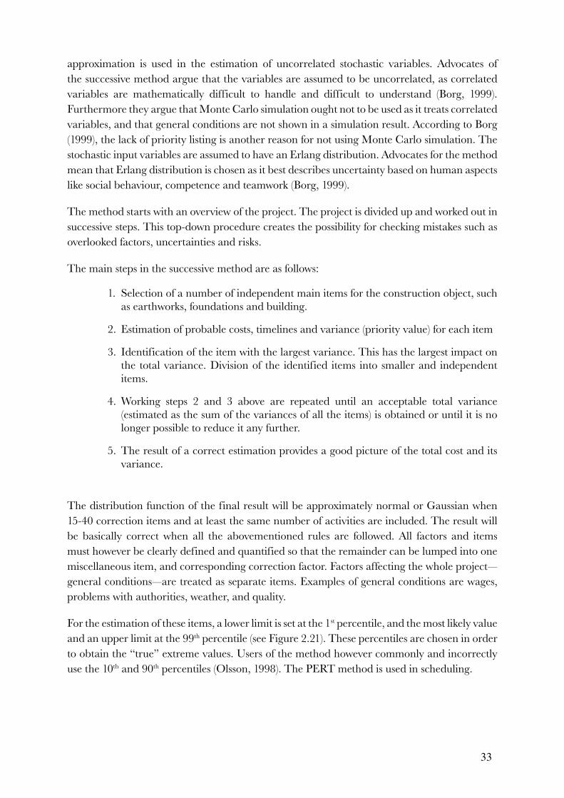
33

approximation is used in the estimation of uncorrelated stochastic variables. Advocates of the successive method argue that the variables are assumed to be uncorrelated, as correlated variables are mathematically difficult to handle and difficult to understand (Borg, 1999). Furthermore they argue that Monte Carlo simulation ought not to be used as it treats correlated variables, and that general conditions are not shown in a simulation result. According to Borg (1999), the lack of priority listing is another reason for not using Monte Carlo simulation. The stochastic input variables are assumed to have an Erlang distribution. Advocates for the method mean that Erlang distribution is chosen as it best describes uncertainty based on human aspects like social behaviour, competence and teamwork (Borg, 1999).

The method starts with an overview of the project. The project is divided up and worked out in successive steps. This top-down procedure creates the possibility for checking mistakes such as overlooked factors, uncertainties and risks.

The main steps in the successive method are as follows:

1. Selection of a number of independent main items for the construction object, such as earthworks, foundations and building.

2. Estimation of probable costs, timelines and variance (priority value) for each item

3. Identification of the item with the largest variance. This has the largest impact on the total variance. Division of the identified items into smaller and independent items.

4. Working steps 2 and 3 above are repeated until an acceptable total variance (estimated as the sum of the variances of all the items) is obtained or until it is no longer possible to reduce it any further.

5. The result of a correct estimation provides a good picture of the total cost and its variance.

The distribution function of the final result will be approximately normal or Gaussian when 15-40 correction items and at least the same number of activities are included. The result will be basically correct when all the abovementioned rules are followed. All factors and items must however be clearly defined and quantified so that the remainder can be lumped into one miscellaneous item, and corresponding correction factor. Factors affecting the whole project—general conditions—are treated as separate items. Examples of general conditions are wages, problems with authorities, weather, and quality.

For the estimation of these items, a lower limit is set at the 1st percentile, and the most likely value and an upper limit at the 99th percentile (see Figure 2.21). These percentiles are chosen in order to obtain the “true” extreme values. Users of the method however commonly and incorrectly use the 10th and 90th percentiles (Olsson, 1998). The PERT method is used in scheduling.

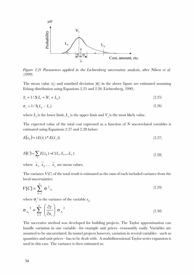
34

Figure 2.21 Parameters applied in the Lichtenberg uncertainty analysis, after Nilsen et al.

(1999).

The mean value (xi) and standard deviation (σ

i) in the above figure are estimated assuming

Erlang distribution using Equations 2.25 and 2.26 (Lichtenberg, 1990).

(2.25)

(2.26)

where Ll is the lower limit, L

u is the upper limit and V

l is the most likely value.

The expected value of the total cost expressed as a function of N uncorrelated variables is estimated using Equations 2.27 and 2.28 below:

(2.27)

(2.28)

where x1,x

2, …x

n are mean values.

The variance V(C) of the total result is estimated as the sum of each included variance from the local uncertainties:

(2.29)

where σz2 is the variance of the variable z

k .

(2.30)

The successive method was developed for building projects. The Taylor approximation can handle variation in one variable—for example unit prices—reasonably easily. Variables are assumed to be uncorrelated. In tunnel projects however, variation in several variables—such as quantities and unit-prices—has to be dealt with. A multidimensional Taylor-series expansion is used in this case. The variance is then estimated as:

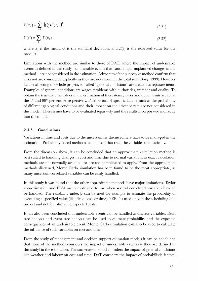
35

(2.31)

(2.32)

wherexi is the mean, σ

i is the standard deviation, and E(z) is the expected value for the

product.

Limitations with the method are similar to those of DAT, where the impact of undesirable events as defined in this study—undesirable events that cause major unplanned changes in the method—are not considered in the estimation. Advocates of the successive method confirm that risks not are considered explicitly as they are not shown in the total sum (Borg, 1999). However factors affecting the whole project, so-called “general conditions” are treated as separate items. Examples of general conditions are wages, problems with authorities, weather and quality. To obtain the true extreme values in the estimation of these items, lower and upper limits are set at the 1st and 99th percentiles respectively. Further tunnel-specific factors such as the probability of different geological conditions and their impact on the advance rate are not considered in this model. These issues have to be evaluated separately and the results incorporated indirectly into the model.

2.3.5 Conclusions

Variations in time and costs due to the uncertainties discussed here have to be managed in the estimation. Probability-based methods can be used that treat the variables stochastically.

From the discussion above, it can be concluded that an approximate calculation method is best suited to handling changes in cost and time due to normal variation, as exact calculation methods are not normally available or are too complicated to apply. From the approximate methods discussed, Monte Carlo simulation has been found to be the most appropriate, as many uncertain correlated variables can be easily handled.

In this study it was found that the other approximate methods have major limitations. Taylor approximation and PEM are complicated to use when several correlated variables have to be handled. The reliability index β can be used for example to estimate the probability of exceeding a specified value (like fixed costs or time). PERT is used only in the scheduling of a project and not for estimating expected costs.

It has also been concluded that undesirable events can be handled as discrete variables. Fault tree analysis and event tree analysis can be used to estimate probability and the expected consequences of an undesirable event. Monte Carlo simulation can also be used to calculate the influence of such variables on cost and time.

From the study of management and decision-support estimation models it can be concluded that none of the methods considers the impact of undesirable events (as they are defined in this study) in the estimation. The successive method considers the impact of general conditions like weather and labour on cost and time. DAT considers the impact of probabilistic factors,

36

technical variables like the capacity of work activities, variables of a more frequently character and cost variables. Monte Carlo simulation and Taylor approximation are used to handle variation in cost and time.

Decisions then have to made based on the results of the calculations, concerning for example the tunnelling method, budgeting and tender pricing. How these decisions can be made, plus the factors affecting these decisions are discussed in the next section.

2.4 Decision making

2.4.1 Introduction

Naturally there are numerous decisions that have to be made regarding tunnel-project planning. Two of the major decisions for every project are establishing:

− the tunnelling method, and − the budget and tender pricing.

Budget and tender pricing are determined by the clients and contractors based on the estimated total cost of each project. Using the estimation system the total cost of a project is expressed as a probability distribution curve. Many factors affect the shape of the distribution curve. Clearly, different tunnelling methods produce different cost curves due to method-specific factors such as the reinforcement measures, machinery and equipment required. The risk factors (relating to normal risk factors and undesirable events) that are considered in the estimation also affect these cost curves. Which of these factors ought to be considered by each party depends on their particular responsibility. Figure 2.22 illustrates outcomes of cost estimation for two different tunnelling methods (A and B). Different decision criteria can be used to choose between tunnelling methods. Deciding budget or tender price is based on the distribution curve of the selected method. The figure also shows one chosen value in the distribution of the tunnelling method.

Figure 2.22 Example of cost distribution for two different tunnelling methods.

It is common practice today for decision makers to determine budget or tender price using deterministic methods. Factors that reduce or increase the value of the estimated total cost are assessed subjectively. By using such an approach, the possible increases in costs and time are not considered in a structured way. Occasionally qualitative, and even less frequently quantitative risk-analysis is used. As cost and time overruns occur often, this may be an indication that this approach to decision-making is inadequate.

37

Naturally, as with making any decision, the alternative that is the most appropriate should be the one selected. Decisions can be made formally using decision-analysis methods, or informally (intuitively).

As there are various parties involved in tunnel projects, psychological factors are important considerations in decision-making. Decision-analysis methods that consider how an individual decision-maker faces a choice involving uncertainties has been discussed in the literature by for example Bell et al. (1988). Three modes of analysis can be considered—descriptive, normative and prescriptive.

A descriptive decision analysis looks at how and why people think and act the way they do. Psychologists have studied how people approach making decisions (the degree of rationality) and whether their behaviour is compatible with any rational model. Another decision-analysis method, concerned more with an abstract, idealised view of how real people make decisions is normative decision analysis. Normative models are evaluated by their theoretical adequacy—the degree to which they provide acceptable conceptualising or rational choice. Prescriptive analysis however describes what an individual logically does in order to make better choices. An example of this method can for example be to point out the necessity of obtaining advice from external experts, and to properly integrate this knowledge with that of others.

Describing all the various decision-analysis methods is beyond the scope of this thesis. However some of the considerations associated with the respective decision analysis methods are discussed in this section along with factors affecting decisions and how making decisions can be based on the output from the estimation model.

2.4.2 Factors affecting decisions

Decisions about the tunnelling method

One of the major decisions in a tunnelling project is deciding on what tunnelling method to use. The probability distribution curve for the estimated total cost and time required for a tunnelling method depends on factors like the type of:

− ground investigation and its extent, − machinery and equipment, − worker profile and experience, − temporary and permanent reinforcement, and − robustness-enhancing measures.

Site and ground investigation are components in one of the key investment strategies for a tunnel project. The results from the ground investigations provide the basis for several essential decisions. The value of increasing the body of knowledge about the ground conditions by conducting additional investigations has been given much attention in the literature (Olsson & Stille, 1980; Sturk, 1998). As the information about the ground conditions in underground construction is always limited and therefore uncertain, there is a need for some way of handling this uncertainty. Bayes’ theorem, combining fundamental and expert geological knowledge,

38

expressed subjectively and combined with observations made during pre-investigation and later during excavation may be a useful tool for this. Such a tool allows the utilisation of the available geological information in the best possible way, thereby reducing uncertainties and facilitating decision-making.

The robustness of the tunnelling method may limit the geological range of application of the method as well as the probability and consequences of undesirable events. The optimal level of geological knowledge or robustness of the tunnelling method depends on many factors, including:

− How much a change in the level of a specific geological factor or robustness affects the limits within which the method works.

− Whether robustness-increasing measures in fact increase the range within which the method works.

− The cost of the investigations. − The cost of the robustness-increasing measures.

The level of robustness and geological knowledge required vary between the different tunnelling methods. Tunnelling using one method featuring high flexibility and direct access to the tunnel face may place different demands on the amount of geological knowledge and robustness than methods with low flexibility and no access to the face.

Clearly, undesirable events causing “exceptional” costs for a tunnelling method have a major effect on the cost distribution curve. It is possible that the client together with a consulting engineer choose the tunnelling method to be used. In designer-built projects, the choice may be made entirely by the contractor. The impact of taking into consideration the party-apportioned responsibility for the extent of exceptional cost when estimating total cost for the tunnelling methods is discussed in the following section.

The responsibility for increases in cost and time that may occur is an important factor for the client as well as the contractor when estimating the total cost for a project. The construction-contracting method involves the type of organisation, payment and award system, affects the responsibility of all the parties involved. If risks are not properly shared, claims and disputes may be some of the consequences during the construction (Reilly et al., 1999). It may also be the case that the contractors add high contingencies to their tenders to cover the costs of identified risks (Charoenngam & Yeh, 1999). Hartman and Snelgrove (1996) indicate that mismanaged risks cause project inefficiencies and make contract relationships adversarial. Furthermore, it is important that all parties have an identical understanding of the risks, as risk contingencies in a tender increase the tender price or extend the schedule, or both (Charoenngam & Yeh, 1999). In this context the following statement from Kleivan and Berdal (1991) becomes of increased interest:

“The main principle of risk sharing in tunnel contracts is to give to the parties a tool for converting work into time-equivalents, a tool with which they can later meet any contingency arising from changed ground conditions, eliminating any future discussions over regulation of the construction time where needed, or over costs incurred. All such problems are foreseen and the answers are to be found in the contract.”

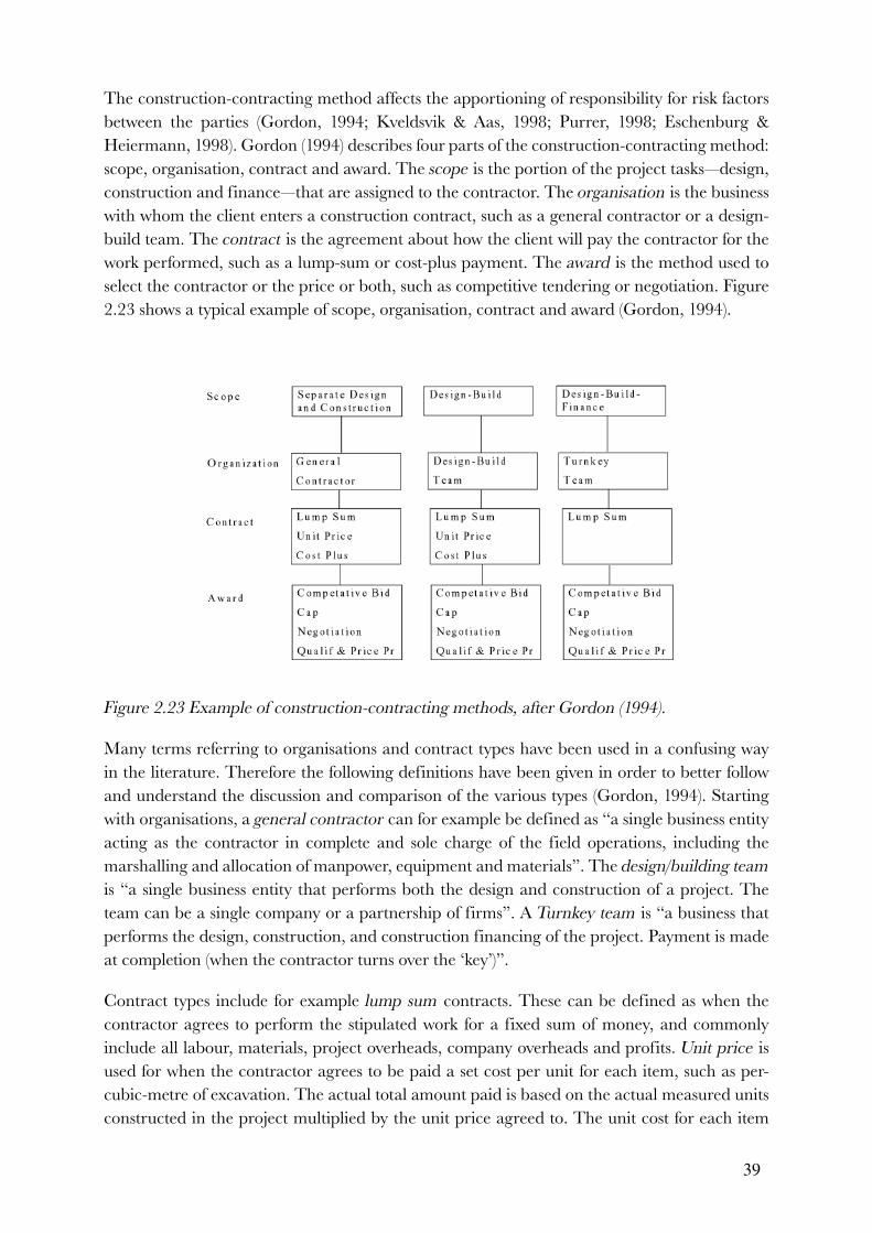
39

The construction-contracting method affects the apportioning of responsibility for risk factors between the parties (Gordon, 1994; Kveldsvik & Aas, 1998; Purrer, 1998; Eschenburg & Heiermann, 1998). Gordon (1994) describes four parts of the construction-contracting method: scope, organisation, contract and award. The scope is the portion of the project tasks—design, construction and finance—that are assigned to the contractor. The organisation is the business with whom the client enters a construction contract, such as a general contractor or a design-build team. The contract is the agreement about how the client will pay the contractor for the work performed, such as a lump-sum or cost-plus payment. The award is the method used to select the contractor or the price or both, such as competitive tendering or negotiation. Figure 2.23 shows a typical example of scope, organisation, contract and award (Gordon, 1994).

Figure 2.23 Example of construction-contracting methods, after Gordon (1994).

Many terms referring to organisations and contract types have been used in a confusing way in the literature. Therefore the following definitions have been given in order to better follow and understand the discussion and comparison of the various types (Gordon, 1994). Starting with organisations, a general contractor can for example be defined as “a single business entity acting as the contractor in complete and sole charge of the field operations, including the marshalling and allocation of manpower, equipment and materials”. The design/building team

is “a single business entity that performs both the design and construction of a project. The team can be a single company or a partnership of firms”. A Turnkey team is “a business that performs the design, construction, and construction financing of the project. Payment is made at completion (when the contractor turns over the ‘key’)”.

Contract types include for example lump sum contracts. These can be defined as when the contractor agrees to perform the stipulated work for a fixed sum of money, and commonly include all labour, materials, project overheads, company overheads and profits. Unit price is used for when the contractor agrees to be paid a set cost per unit for each item, such as per-cubic-metre of excavation. The actual total amount paid is based on the actual measured units constructed in the project multiplied by the unit price agreed to. The unit cost for each item

40

commonly includes all labour, materials, project overheads, company overheads and profits. Sometimes overhead items are paid separately. Cost-plus is when the contractor is reimbursed for the cost of doing the work, including the labour, materials, and project overheads, plus a fee including company overheads and profits. The fee can be a fixed sum—such as a percentage of the cost—or a formula incorporating both. When it comes to “award”, the competitive tender

is commonly used. Using this method a contractor is selected on the lowest price proposal in market competition. The term cap is used when a fixed price or cap is set by the owner against which contractors competitively propose a level of quality and options for a project. Negotiation is when the price or contractor or both are selected by negotiations between the owner and one or several contractors. Qualification and price proposal is when contractors are competitively selected based on their qualifications and price. The process is often quantified with a ranking formula.

The above-defined terms organisation, contract and award are applied in different combinations in construction-contracting methods in tunnel projects. The clients’ and contractors’ responsibilities for increases in costs and time due to different risk factors depend on the construction-contracting method applied. The responsibility for risk factors such as construction, physical, performance and financial (see Table 2.1) have been discussed elsewhere in the literature (Purrer, 1998; Pellar & Watzlaw, 1998; Eschenburg & Heiermann, 1998; Tengborg,1998). As already discussed, the factors causing changes in cost and time can be divided into “variation caused by normal risk factors”, plus “undesirable events” and “abnormal events” caused by abnormal risk factors.

For general contractors, construction-related risk factors like deviations in construction documentation for planning, drawings, descriptions and designs are normally borne by the client as the provider of this material (Lindgren, 1981). For design-build and turnkey contract teams however, the responsibility for design and construction details are transferred to the contractor. If the client wants to modify or add to the work, the lump sum has to be re-estimated (Lindgren, 1981). In the literature it is suggested that deviations in actual quantities of for example construction materials are handled as construction risks. However in tunnelling projects, the ground conditions have a major impact on these quantities. Consequently deviations in quantities are often handled as physical risks (Pellar & Watzlaw, 1998).

Client and contractor responsibility for selecting TBM characteristics has been discussed in the literature by Reilly (1997). As tunnelling machines are becoming increasingly specific and complex, the selection of the correct machine characteristic plays an important role in the success of a project. Experience from the United States shows that a prescriptive approach, where the client (advised by experts) fully defines the type and characteristics of the machinery and the support measures, is more advantageous than a performance approach where the general contractor is free to choose, being required only to meet the key project performance requirements given by the client. Clearly in design-build or turnkey approaches, the experienced contractor would be best suited to determining the most appropriate methods and techniques. In a low-tender environment however, a general contractor is often not willing to select a sophisticated machine, but rather the cheapest considered capable of constructing the tunnel. An inadequate and cheap machine may however result in major cost and time increases (Reilly,

41

1997). However, experience from Europe show that cost and time may be reduced where the general contractor is free to select equipment or machinery, compared to those proposed by the client (Aebersold, 1994). The award system applied should therefore affect which of the parties involved should be responsible for TBM characteristics.

As previously discussed, undesirable events are often connected to geological and hydrogeological conditions and are therefore physically-related risks. The client is often responsible for the site conditions and therefore for risks associated with the encountering of site conditions diverging from those originally defined by client (ITA, 1988). The client therefore often has the main responsibility for physical risk factors like the geological and hydrogeological conditions responsible for causing exceptional costs. When using lump-sum contracts however, the client tries to put as much risk as possible onto the contractor as an incentive for productivity. This often results in raising the cost of the contracts. If the responsibility relationship between client and contractor is not clear, disputes may occur. Experience shows that responsibilities for geological conditions are less expensive when borne by the client, who is normally the major financial strength in the project (Purrer, 1998). Usually when applying unit-cost contracts, the client has the main responsibility for deviations in quantities. The contractor may re-estimate unit prices when the actual quantities differ considerably, for example by more than 10-25% from the estimated ones. Due to the complex and uncertain conditions prevailing in tunnelling projects, there is however a demand from the client to use modified contract types in addition to the unit-price-contracting system, where the contractor has the responsibility for the quantities of support measures (Pellar & Watzlaw, 1998). In some other modified contracting methods it is possible for some cost increases to be transferred from the client to the contractor, where these are under the contractor’s control (Purrer, 1998; ITA, 1988). Reasons for these sorts of cost increases may include for example: deviations between actual and estimated overbreak, the consumption of shotcrete or explosives or drilling steel, the amount of work hours spent on support measures, and the amount of time-dependent costs in establishing the site.

Financial risk factors like funding and national or international impacts are normally borne by the client, who bears the ultimate responsibility for financing and commissioning the projects (Reilly, 1997). Responsibility for the impact of the market situation on prices of materials, wages and equipment is normally borne by the contractor, independent of the construction-contracting method, as this can be seen as being a “normal risk factor”. If however prices vary significantly and unpredictably, the contractor will either, (a) overestimate this risk with the client having to pay more than necessary for the work, or (b) underestimate the risks, which may lead to financial loss. Contract provisions protecting the contractor can however be used to reduce this type of risk (ITA, 1988).

Performance-related risk factors like the capacity of machinery and labour are normally the responsibility of the contractor, as these are usually under the contractor’s control. These factors can be seen as “normal risk factors”.

Figure 2.24 shows an example of risk sharing between client and contractor for different sorts of contracts (Kveldsvik & Aas, 1998). According to Kveldsvik and Aas, the minimum project cost is always obtained where the so-called “Norwegian Practice” of risk sharing between client

42

and contractor is used. Of course this is subjective, with no proof available. When the actual ground conditions differ a lot from the prognosis, or when the geotechnical reports contain insufficient information, severe conflicts may arise between the parties. The client may argue that the flexibility contained in the contract system is unlimited, but the contractor may claim extra compensation.

Figure 2.24 Risk sharing according to the type of contract and assumed influence on project

cost, after Kveldsvik & Aas (1998).

Responsibility for the various different risk factors must be clearly apportioned to the client and contractor respectively in every tunnelling project. There may however be areas where each party’s responsibility for increases in cost and time is not quite clear. An example of such an area is the responsibility for the actual quantities of construction materials used when a lump-sum contract is in place. In this case, the contractor is normally responsible for any increases in the quantities of construction materials. If however, there is a major increase in the quantities required, the responsibility may be transferred to the client. When working out party responsibilities in a structured way, the chances of recognising areas containing inadequate division of responsibility can be increased.

Table 2.6 illustrates some general examples of risk factors where the contractor may have the major share of the responsibility in cases where there is a deviation in actual compared to estimated conditions, depending on the construction-contracting method. The examples seen in the table are based on literature studies and the experience of the author. Clearly there may be other opinions about who bears the main responsibility for the risk factors listed.

43

Table 2.6 Examples of responsibility for different risk factors depending on the construction-

contracting method, where x is the responsibility borne mainly by the contractor, (x) is partly

the contractors responsibility, L-s is a lump-sum contract, U-p is a unit-price contract, and

C-p is a cost-plus contract.

Risk factor

Organisation

Contract

General

contractor

L-s U-p C-p

Design-build

team

L-s U-p

Turnkey

team

L-s

Normal-risk factors

Physical-risk factors

Subsurface geological and hydrogeological conditions

x x . x x . x

Deviation in actual quantities x (x) . x (x) . x

Financially-related risk factors

Market situation x x . x x . x

Construction-related risk factors

Deviation in construction documentation

x x . x

Performance-risk factors

Capacity of machines and labour x x . x x . x

Undesirable event

Physical-risk factors

Subsurface geological and hydrogeological conditions

(x) . x . x

Actual quantities of work (x) . x . x

Figure 2.25 illustrates possible distribution curves of total cost versus construction-contracting method. For a contractor with limited responsibility (for example a general contractor with a unit-price contract) it may be sufficient to simply consider the variation due to normal risk factors in cost and time, as the exceptional costs due to undesirable events may be covered by insurance or specific claims (A in Figure 2.25). Tunnel projects are however increasingly moving toward lump-sum contracts (Andreossi, 1998). In these cases the contractor bears an increased responsibility and the possibilities for contractors to claim for increased costs are restricted. It may therefore be necessary to consider some exceptional costs that may occur due to undesirable events (B in Figure 2.25). For the client bearing the responsibility for financing the project, it may be necessary to consider all the possible exceptional costs due to undesirable events (C in Figure 2.25). In some cases it may also be necessary to include exceptional costs due to “abnormal risk factors” in the budget.

Figure 2.25 Different decision-making-outcome ranges depending on the responsibilities of

each of the respective decision makers.

44

Decision about tender price and budget

There are numerous different factors affecting client and contractor decisions about budget and tender pricing. The following are taken from Hintze (1994), Kastjberg (1994) and Reilly (1996):

− political interest, − the purpose of the decision, − laws and regulations, and − risk acceptance.

The parties involved in the construction process have different decision-making objectives. The objective of those parties carrying out budget determination may be to get a project started. Political pressure to get a project started may affect the client when determine the budget. It may be the case sometimes that lower budget figures are chosen instead of more realistic costings that including risk factors.

The pitch of the tender price can be determined in order to win a contract and make a profit, or to become known by the client, or even just to show a general interest in the project. Factors such as laws and regulations also affect the client as well as contractor’s chances of winning claims. The consequences of for example incorrect design or faulty workmanship, which can result in large claims, are however increasingly transferred to insurance companies (Andreossi, 1998).

The contractor’s level of risk acceptance is an important factor when the tender price is being determined. The tender price must on one hand be low enough for the contractor to have a reasonable chance of winning the contract in a tough competitive pricing environment. On the other hand it must be high enough to cover the construction costs and losses that may have occurred in other projects, as well as to be able to return a certain level of profit. Due to tough contract competition and low tender evaluation criteria, contractors are often required to take a higher risk than they either wish to or have the capacity to do.

Other factors affecting risk acceptance, such as prestige, shortage of time and misunderstandings have been discussed in the literature. Using knowledge about the risk acceptance of each of the decision makers, it is possible to define a specific risk-acceptance function. Depending on the cost that a decision maker is willing to pay for avoiding risk, various different risk categories can be defined (Benjamin & Cornell, 1970). This can basically be described as the fictive cost to be used in risk estimation. A decision maker whose decisions are “risk-averse”, adopts a negative risk premium position, and a decision maker whose decisions are “risk-seeking” adopts a positive risk premium position (see Figure 2.26).

45

Figure 2.26 Illustration of the risk acceptance of a risk-taking, a risk-neutral and a risk-averse

decision maker on the basis of the risk premium, after Högberg and Edlund (1986).

Most decision makers exhibit a reference point, above which their behaviour is risk averse and below it, is risk seeking. It has been observed that people do not distinguish between large values adequately, and that larger risks are often accepted when the benefits are great (Bell et al.,1988).

The abovementioned factors impact on how the final decisions about budget and tender price are made. In the following section, different decision-analysis methods and criteria are discussed.

2.4.3 Decision-analysis methods and criteria

General aspects

The total time and cost of a tunnelling method can be described using a distribution curve. To choose a tunnelling method, decision-analysis methods and criteria for choice between the distributions are needed. To determine a tender price or budget requires the application of decision-analysis methods and criteria for choice of one value in a distribution. Most decision methods and criteria used today mainly concern decisions between values rather than distributions, or a value in a distribution (Hillier & Lieberman, 1995; Benjamin & Cornell, 1970). An overview of the commonly used decision-analysis methods and decision criteria will be briefly described below.

Hillier & Liebermann (1985) provide the following decision criteria able to be used for deciding between certain values:

− the maximum pay-off criterion, − the maximum likelihood criterion, and − the Bayes’ decision criterion.

When the decision maker has to select one action for proceeding with the problem at hand, and each of the action alternatives refers to a possible “state of nature”, profit or loss could be

46

used as a quantitative measure of the consequences of the outcome. A table is commonly used to provide the profits or losses for each combination of actions and the state of nature.

When using the maximum pay-off criterion, the minimum profit or loss over all possible states of nature have to be found first. Then the maximum of these minimum profits can be identified. The action that gives this maximum pay-off is chosen. This decision criterion is normally of interest only to very cautious decision makers.

The maximum likelihood criterion focuses on the most likely state of nature (the state with the greatest probability). The action is then chosen which has the maximum profit for this state.

One commonly used criterion is Bayes´ decision criterion. The expected outcome is estimated from the probability and consequences of a particular state of nature. The best available estimates of the probabilities of the respective states of nature are used when estimating the expected value of the profit and loss for each of the possible actions. The action with the maximum expected profit and minimum expected loss is chosen. An advantage with this criterion is that all the available information is used (Hillier & Lieberman, 1995).

When the decision involves choosing between different alternatives, a decision tree analysis is employed to find the best alternative (Benjamin & Cornell, 1970; Ang & Tang, 1985). The trees are very useful when a sequence of decisions has be made. In the analysis, the financial flow along the paths of the tree and the total cost at the end of the tree are shown (Haimes, 1998; Benjamin & Cornell, 1970). The method is described in the literature and applied to enable the comparison of single outcomes.

There are many data inputs required in a decision tree analysis. These input data often contain uncertainties. To reduce the uncertainty, additional information can be used. According to Benjamin & Cornell (1970), the engineer may use the following measures:

− extending investigations of the ground such as core drillings and seismic investigations,

− interviewing a representative group of people, and − installing measuring equipment to collect a range of observations.

The additional information however adds extra costs, and this new information must be included in the decision analysis (Olsson & Stille, 1980; Ang & Tang, 1984).

Figure 2.27 shows an example of the impact of additional cost information and exceptional costs due to undesirable events for two tunnelling methods. The nodes of the decision tree represented by a square indicate that a decision needs to be made at that point. A circle indicates that a random event occurs at that point.

47

Figure 2.27 Example of a decision tree, after Hillier & Lieberman (1995).

Decision about tunnelling method

The minimum expected total cost (min E[C]) is one example of Bayes’ decision criteria which can be used for decision between distribution curves (Benjamin & Cornell, 1970). However using just the expected value as a decision criterion often leads to erroneous conclusions and misunderstandings in the decision-making (Haimes, 1985). The decision about which tunnelling method to use may therefore not necessarily be just a matter of finding the one with the lowest expected cost. Instead it may also involve considering the variation or probability or both of exceeding a certain value. In some cases, when one method (A) has a lower mean value but a larger variation than another method with a higher mean value but smaller variation (B) it may be preferable to choose the method with the smaller variation (see Figure 2.28).

Figure 2.28 Example of distribution curves of total cost for different tunnelling methods.

The probability of exceeding a certain limit can be estimated by using probability theory or reliability index β. Figure 2.29 illustrates a comparison of cumulative distribution curves

48

obtained by Monte Carlo simulation. The figure shows that the probability of exceeding the total cost “I” is lower for tunnelling method B than for method A.

Figure 2.29 Illustration of the cumulative distribution of total cost for tunnelling methods A

and B.

Psychological factors may also affect the choice of tunnelling method. It has been observed that risk acceptance tends to be lower in connection with new techniques than with widely used ones (Bell et al.,1988).

Once deciding on a tunnelling method, the exact cost of the tender or budget has to be determined based on the cost distribution curve for the chosen method.

Decision about tender and budget pricing

Different criteria can be used to determine the values of the tender and budget from the distribution curve of the total cost of the chosen tunnelling method.

One possible decision criterion to use for choosing tunnelling method based on a distribution curve is to check the probability of exceeding a certain total cost or time value. Figure 2.30 shows a cumulative distribution curve for a chosen tunnelling method.

Figure 2.30 Illustration of cumulative distribution of total cost for a tunnelling method.

The probability of exceeding a certain cost or time value can also be estimated using the

49

reliability index β mentioned in Section 2.3.2.

One method to use to decide budget or tender price is the “Partitioned Multi-objective Risk Method” or PMRM (Haimes, 1998). This was developed as people tend to concentrate on risks with low probabilities and many consequences instead of risks with higher probabilities but fewer consequences. The PMRM generates a number of conditionally-expected value functions, called “risk functions” instead of using the traditional expected risk value. The risk functions represent the risks given that the associated consequences do not exceed the specific probability range (Haimes, 1998). In the PMRM a family of risk measures for each decision strategy is provided. The partitioning of risk into three ranges of consequences is illustrated in Figure 2.31. On a plot of “exceeding probability”, there is a unique value for damage β

1 on the consequence

axis that corresponds to the exceeding probability (1- α1) on the probability axis. Similarly,

there is a unique value for consequences β2 that corresponds to the exceeding probability (1-α

2).

Damages of less than β1 are considered to be of low severity, and consequences greater than β

2

are of high severity. Similarly, consequences of magnitude between β1 and β

2 are considered to

be of moderate severity.

Figure 2.31 Partitioning of risk into three severity ranges, after Haimes (1998).

The decision criteria mentioned can be used for determining one value, for example the tender or budget pricing based on a distribution.

2.4.4 Conclusion

The total cost of a tunnelling method is expressed as a distribution curve. Which particular tunnelling method and risk factors that are considered in the estimation affect the distribution of the total cost of a tunnelling method. The responsibilities of the respective parties (client and contractor) for increases in cost and time that may occur due to various risk factors depends on the construction-contracting method as well as the stage of the project. Decisions about which tunnelling method to use are really decisions about different distributions of time and cost. From this decision the budget and tender prices have to be determined by the client and

50

the contractor respectively. Choosing the tunnelling method requires decision-analysis methods and criteria that consider distribution. Commonly used decision-analysis methods and criteria are often adapted to decide between certain values. There are however methods available for deciding on the tunnelling method, and the tender or budget pricing. The criterion for deciding on the tunnelling method is not always the minimum-expected total cost and time; the probability of exceeding a certain value is also an important consideration in the decision.

PMRM can be used to determine tender or budget pricing. This method is suitable as it generates a number of conditionally-expected value functions called “risk functions” instead of the commonly used expected value.

2.5 Conclusions regarding the demands on estimation models

This chapter has been devoted to discussing the demands on an estimation model for tunnel projects. One conclusion of the findings is that the tunnelling process is a “serial” production system in two senses. Firstly, the possibilities for changing the work site are limited, except where more than one tunnel adit is made. Secondly, the possibilities for executing more than one main work activity at a time are limited. Disturbances therefore often have larger impacts on the time and cost budgets in tunnel projects than in other types of construction projects.

Various studies, for example by Kastbjerg (1994), Andreossi (1998), and HSE (1996) have shown that major cost and time overruns are common in infrastructure projects including tunnelling. As these overruns cause major problems for all the parties involved in the tunnelling process, it is important to consider the risk factors that may be causing these cost and time overruns in a structured way in the estimation of cost and time for these sorts of projects.

Based on the analysis of the various different risk factors and their impacts on cost and time in tunnelling projects, it has been concluded that it is important to clearly separate normal and exceptional cost and time variables. Current decision-support estimation models (such as the Successive method and DAT), which handle variations caused by these variables, do not treat normal and exceptional costs and time separately in the estimation.

In this study variation due to normal risk factors are defined as “factors causing deviations in the normal span” of the project. Examples of normal risk factors are performance-related factors such as efficiency and productivity of equipment and labour, and financially-related factors such as market conditions.

In this study undesirable events are defined as “events that cause major unplanned changes in the tunnelling process”. Undesirable events often occur as a result of physical factors like geological and hydrogeological conditions. These events can for example include tunnel collapses and other damage that can lead to the total modification or termination of excavation via the initial method due to unforeseen changes in the geological conditions.

In the study robustness means flexibility and preparedness to meet the actual conditions encountered. Based on case studies by for example Hentschel (1997), Wenger (1994), and Beck and Thullner (1998), it can be concluded that the application of specific measures to increases

51

the robustness of the tunnelling method actually influences the occurrence of undesirable events. Robustness therefore ought to be taken into consideration in the estimation.

Undesirable events caused by abnormal risk factors, such as an act of God—earthquakes, hurricanes and the like—ought not to be taken into consideration in the estimation of cost and time for a tunnel project. The consequences of abnormal risk factors are normally covered by insurance.

It can be stated that the construction-contracting method as well as the stage of project determine which party (the client or contractor) is responsible for the increases in cost and time occurring as a result of the various risk factors (Kveldsvik & Aas, 1998; Purrer, 1998; Eschenburg & Heiermann, 1998). Clearly, the client normally has the ultimate responsibility for financing the project. It may however be appropriate for some of the costs resulting from the risks to be borne by the contractor. The contractor often carries increases in cost and time due to normal risk factors, as these are mainly under the contractor’s control. Exceptional costs and time resulting from undesirable-event-related risk factors are normally borne by the client, who is generally the major financier, but in some cases the costs are shared between the parties.

Estimations are usually made using deterministic methods (Quellmetz, 1987). There is however a need to handle variation in cost and time variables in the estimations.

It can be concluded that an approximate calculation method would be best suited to handling variations in cost and time due to normal risk factors, as exact calculation methods are normally non-existent or become very complicated. From the approximate methods discussed, Monte Carlo simulation is deemed appropriate, as many uncertain correlated variables can be easily handled. Undesirable events can be handled as discrete variables. Fault tree analysis and event tree analysis can be used to estimate the probability and expected consequences of an undesirable event.

As the total cost for a tunnelling method is expressed as a distribution curve, deciding about which tunnelling method to use is a decision between different distributions of time and cost. Based on these decisions the budget and tender price have to be determined by the client and contractor respectively. Decision-analysis methods and criteria that consider distribution are required for choosing a tunnelling method. Commonly used decision analysis methods and criteria are often utilised for deciding between certain values. There are however methods for deciding on the tunnelling method and tender and budget pricing. The criterion for deciding on the tunnelling method is not always the minimum expected total cost and time; rather the probability of exceeding a certain value is also an important consideration in the decision.

Finally it can be concluded that the client and the contractor face the same problems, and that the decision about both budget and tender pricing has to be made using the same basis. Decision-making for both parties requires the support of a common base, being the distribution of total cost and time. Using an estimation model that provides an overview of the likely costs and time for the project—normal cost and time—and exceptional cost and time, can be one step toward improving the basis for making these decisions.

52

The next chapter presents characteristics of tunnelling methods affecting time and cost estimation.

53

3 Characteristics of tunnelling methods affecting time and cost

estimation

3.1 Introduction

As discussed in chapter 2, the total time and cost for a project can be expressed as normal and exceptional time and cost. The estimation of these time and cost is based on the tunnelling method considered to use. As every project is unique in its purpose and environmental circumstances, it is important to consider factors that may impact the actual tunnelling method in the actual conditions and thereby also the time and costs. The factors can be e.g. applicability of the method, advance rate, undesirable events or robustness of the method. These factors have been discussed in the literature, Maidl (1994) and Girmscheid (2000). The aim of this chapter is to make as a literature survey of these factors and not a detailed study.

The applicability of the tunnelling method is affected by e.g. the excavation technique, geological and hydrogeological conditions.

The advance rate of the tunnelling method is one important factor affecting the normal time and cost. Advance rates for different tunnelling methods and case studies from different methods and geological conditions will therefore be described in this chapter.

Undesirable events of various types often occur in tunnelling projects. The consequences of the events impact the time and cost of the project, and are therefore important to consider in the estimation. To be able to estimate the time and cost caused by the undesirable events, they have to be identified. Which undesirable events that may occur using conventional methods and tunnelling machine are discussed in this chapter. As the importance to consider risks in the estimation of project time and cost, are stressed in this thesis, the discussion about undesirable events is more extensive than factors affecting normal time and cost.

Robustness-increasing measures can be applied in order to increase the geological field of application as well as the advance rate of tunnelling methods. Various robustness-increasing measures are therefore discussed in this chapter.

Each of the factors affecting time and cost will in this chapter be exemplified with case studies for different tunnelling methods. The tunnelling methods exemplified have been be divided into two main groups:

− those that use conventional methods such as drilling and blasting, and road headers and diggers, and

− those that use tunnelling machines such as TBMs and shielded machines.

Figure 3.1 provides an overview of various tunnelling methods.

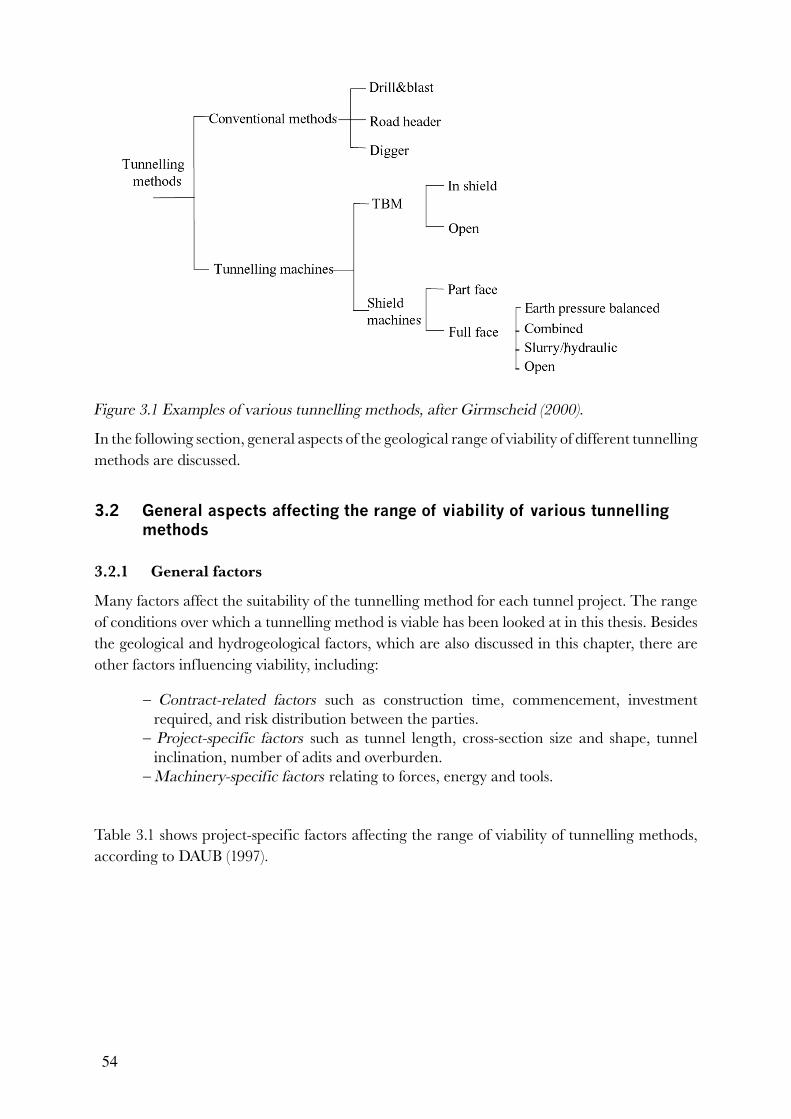
54

Figure 3.1 Examples of various tunnelling methods, after Girmscheid (2000).

In the following section, general aspects of the geological range of viability of different tunnelling methods are discussed.

3.2 General aspects affecting the range of viability of various tunnelling methods

3.2.1 General factors

Many factors affect the suitability of the tunnelling method for each tunnel project. The range of conditions over which a tunnelling method is viable has been looked at in this thesis. Besides the geological and hydrogeological factors, which are also discussed in this chapter, there are other factors influencing viability, including:

− Contract-related factors such as construction time, commencement, investment required, and risk distribution between the parties.

− Project-specific factors such as tunnel length, cross-section size and shape, tunnel inclination, number of adits and overburden.

− Machinery-specific factors relating to forces, energy and tools.

Table 3.1 shows project-specific factors affecting the range of viability of tunnelling methods, according to DAUB (1997).

55

Table 3.1 Example of project-specific factors affecting the range of viability of tunnelling

methods

Factor

Tunnelling method

Size ofcross

sectionUniform

Size of cross

sectionVariable

Form ofcross

sectionUniform

Form of cross section

Variable

Tunnel length

Short

Tunnel length

Long

Conventional methods

X X X X X X

Tunnelling machines

X O Circular O - X

X=well suited, O= not suited, -=not usual

Conventional methods are flexible, as they allow changes in the shape and size of the cross section and installation of rock supports such as shotcrete, bolts and steel arches during the excavation process. Due to low investment costs the methods can be used for both short and long tunnels. Conventional methods however require experienced workers.

Due to high investment costs tunnelling machines are mostly used in long tunnels. The work environment is often better than with conventional methods. The flexibility for accommodating variation in ground conditions or changes in the cross section however is low. It is also difficult to apply rock-support measures when the tunnel diameter is small. Extensive knowledge about the geotechnical characteristics of the site is necessary for choosing the correct face support. A relatively large space is required in front of the tunnel face for installing the machine (Müller, 1978).

Figure 3.2 shows the dependence between cost and tunnel length for different tunnelling methods. The tunnelling method with the lowest cost for each respective tunnel length is marked in the figure.

Figure 3.2 Dependence between cost and tunnel length for different tunnelling methods, after

Girmscheid (2000).

56

Properties like cuttability determine the efficiency and capacity for rock cutting with drag bits. Drillability determines the efficiency and capacity for cutting with roller cutters. The abrasiveness of the ground determines the wear and tear on the tools being used.

The range of geological conditions wherein the method can be used is determined by the excavation principle—the way the tunnel is excavated, the rock support measures, and the mucking-out system. The geological range of viability for different tunnelling methods is discussed in the following section.

3.2.2 Examples using different tunnelling methods


Conventional methods do not employ mechanical supporting of the tunnel face. Figure 3.3 illustrates excavation using a drill-and-blast method and road header.

Figure 3.3 Excavation using a drill-and-blast method and road header, Girmscheid (2000).

Various factors affecting the range of viability of conventional methods have been discussed in the literature by for example Gehring (1997). The following geological factors are considered to be important:

− the quality, stability and stand-up time of the rock mass, − the abrasiveness of the rock mass, and − the presence of water in the rock mass.

The quality of the rock affect the cross-section possible to apply (see Figure 3.4).

Figure 3.4 Possible tunnel profiles depending on the quality of the rock.

57

The quality of the rock also dictates the excavation principle and rock-support measures that can be used (see Figures 3.5 and 3.6.) Excavation can be done in a number of ways: full face, heading and bench or partial face (multiple drift). Dividing the excavation into partial sections with rounded-base heading can be done in order to reduce the stresses in the edges. The number of partial sections used depends on the size of the cross section and the rock quality. The distance between the heading and the closed section can be varied using a partial construction method. The section closing is defined as long if the distance between the face of the heading and the closed section is 50-200 m, and short if the distance is at 30 m or less.

Figure 3.5 Full face, heading and bench, and multiple-drift excavation cross-sections.

If the rock quality is very poor, partial-face excavation with a support core is required for increasing the stability of the tunnelling (see Figure 3.6). These sorts of conditions also require that the section be closed fast and short round-lengths to be used.

Figure 3.6 Multiple drift with support core and grouted piles.

The abrasiveness and compressive strength of the ground determines the possibility of using conventional methods. Figure 3.7 gives an indication of the ranges where drilling-and-blasting and road-header methods can be used. With regard to drilling and blasting, the defined range is only valid for drilling with a normal small borehole diameter.

58

Figure 3.7 Ranges of viability for using drilling-and-blasting and road-header methods, after

Girmscheid (2000).

Conventional methods have a limited application below the groundwater table where there may be flowing ground, and in areas with thin overburden and weak rock where there may be sinkholes or old boreholes. Certain fine-grain, saturated soils with thixotropic behaviour must be dewatered with vacuum wells where they occur in the section to be excavated or just above it. Here the limit of method applicability is reached for tunnelling without mechanical face support.

Tunnelling machines

Tunnelling machines can be used in dry as well as water-bearing rock and soil. Factors affecting the range of viability for tunnelling machines have been discussed in the literature by for example Maidl (1994), Barbendererde (1991) and Girmscheid (2000). The following are important factors in determining their use:

− conductivity of the soil and rock, − water pressure, and − grain-size distribution of the soil.

Figure 3.8 illustrates the impact of these factors on the range of viability for tunnelling machines (Mignonat, 1996).

59

Figure 3.8 Field of use for various shield machines determined by conductivity, water pressure

and grain-size distribution, after Mignonat (1996).

TBMs are able to be used in rock (see Figure 3.9). The TBM is driven forward against the rock face by grippers, and rock support can be applied behind the bore head if necessary.

Figure 3.9 Tunnel boring machine

Tunnelling with TBMs is normally used in rock with a uniaxial compressive strength of about 60-300 MPa (DAUB, 1997). At higher strengths, and higher abrasive-rock contents the method becomes less profitable. The shear strength of the rock ( ) should ideally be about 5-25 MPa and the Rock Quality Design (RQD) about 50-100%. The joint distance should be less than 0.6 m. It is however possible, despite the problems, to use TBMs in less favourable conditions, for

60

example at lower compressive strengths down to about 20 MPa, joint distances of about 0.2 m, RQD of about 20%, and tensile strengths up to 2 MPa.

Figure 3.10 shows the range of viability in abrasiveness of the ground and the compressive strength for TBM

Figure 3.10 Range of viability for TBMs in rock, after Girmscheid (2000).

In soil-like conditions, different types of shielded machines can be used ( Maidl et al., 1994; Müller, 1978). Shielded machines are pushed forward by hydraulic jacks working against pre-cast concrete segments installed every round (see Figure 3.11).

Figure 3.11 Typical pre-cast concrete segment, after Schmid (1994).

These segments are usually made of watertight concrete and are between 25-50 cm thick. The segments are required to be durable, highly accurate and strong enough—especially when only one layer of segments is used—to immediately support all the prevailing soil and water pressures (Schmid, 1994). Due to the weight involved, the segments are installed with erectors. The space between the concrete segments and the surrounding ground is grouted. Table 3.2 shows geological parameter values suitable for using tunnelling machines.

61

Table 3.2 Geological parameter values for using different tunnelling machines, after DAUB

(1997).

Rock mass A B C D E F

Geotech. param.

Compressive strength

[MN/m2]

50-300 5-50 1.0 0.1

Tensile strength

[MN/m2]

5-25 0.5-5

RQD value [%] 50-100 10-50

Joint distance [m] 0.6 to >2 0.06-0.6

Cohesion [kN/m2] >30 5-30 5-30

Grain distribution

<0.02 [%]

<0.06 [%]

30

>30

30

>30

10

Type of tunnelling

machine

TBM agw gw

xx

oo

TBM - shield agw gw

oo

xx

Open shield agw gw

oo

ox

x

EPB shield agw gw o x o oSlurry shield agw gw

o oo

ox

Excavation tool Rollingcutter disc

Rollingdisc bit

Strippingflat bit

Strippingchisel bit

Looseningflat bit

Looseningpick

Note: agw means without or above the groundwater, gw means with or below the groundwater, x is the main

range of viability for the method in the given range of rock-mass parameters, o means that the application of the

method is possible in the given range of rock-mass parameters. Rock masses: A means that the ground conditions

vary between stable rock and showing signs of caving in; B varies between caving in (tends to brake in “gebräch”)

and unstable; C means cohesive and stable; D means cohesive and not stable; E means the conditions are mixed;

and F means that the rock mass is not cohesive.

It is important to select the proper cutting tools for the machine being used. Drag bits must be used in unconsolidated ground, and cutters for crushing hard rock. Using cutters ought to be avoided where not required, as the costs of wear and tear on the cutters are high. However hitting hard rock with a machine that is not equipped with cutters may result in major problems. If the geological conditions vary, especially where for example soft ground contains boulders, a combination of different tools may be needed. Figure 3.12 shows different types of tools used for boring.

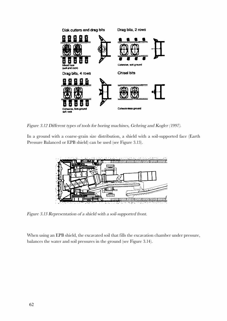
62

Figure 3.12 Different types of tools for boring machines, Gehring and Kogler (1997).

In a ground with a coarse-grain size distribution, a shield with a soil-supported face (Earth Pressure Balanced or EPB shield) can be used (see Figure 3.13).

Figure 3.13 Representation of a shield with a soil-supported front.

When using an EPB shield, the excavated soil that fills the excavation chamber under pressure, balances the water and soil pressures in the ground (see Figure 3.14).

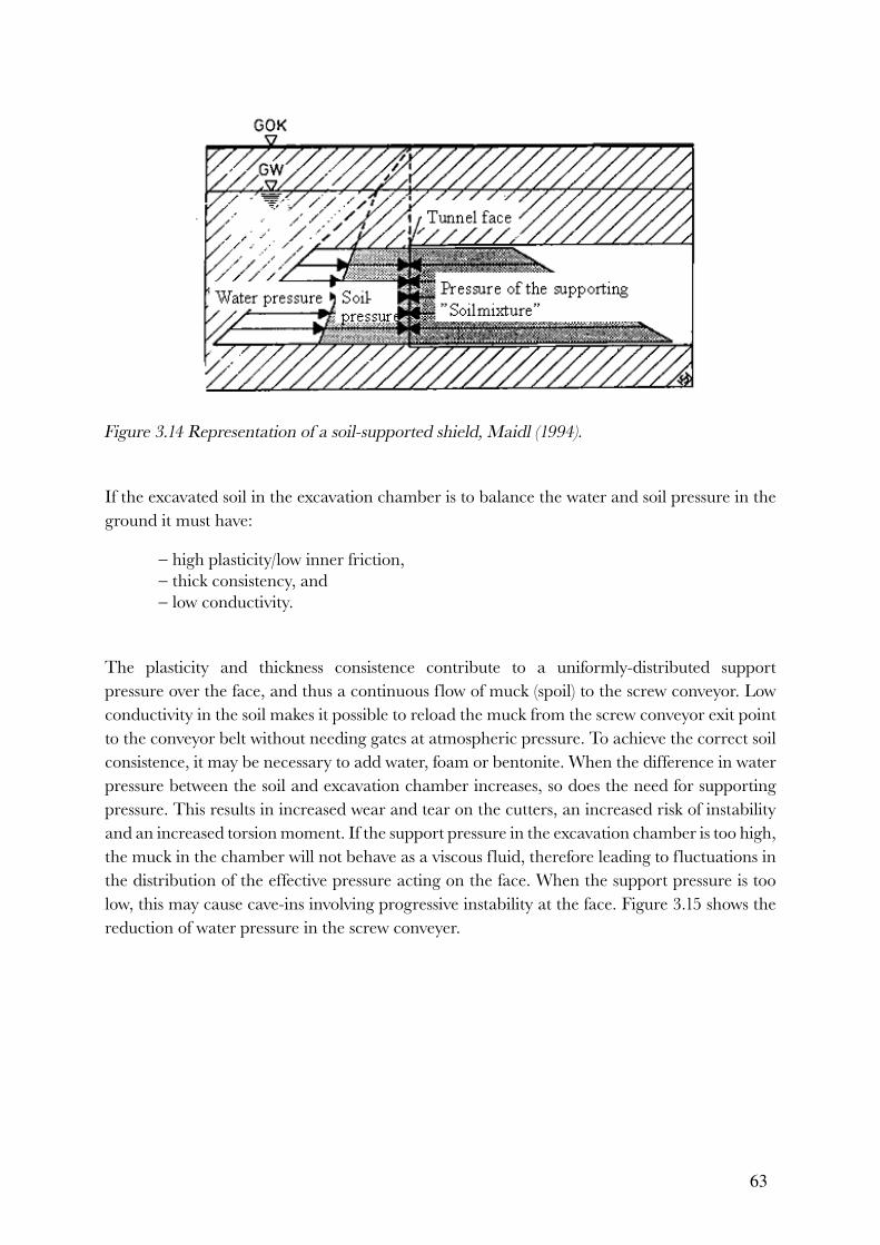
63

Figure 3.14 Representation of a soil-supported shield, Maidl (1994).

If the excavated soil in the excavation chamber is to balance the water and soil pressure in the ground it must have:

− high plasticity/low inner friction, − thick consistency, and − low conductivity.

The plasticity and thickness consistence contribute to a uniformly-distributed support pressure over the face, and thus a continuous flow of muck (spoil) to the screw conveyor. Low conductivity in the soil makes it possible to reload the muck from the screw conveyor exit point to the conveyor belt without needing gates at atmospheric pressure. To achieve the correct soil consistence, it may be necessary to add water, foam or bentonite. When the difference in water pressure between the soil and excavation chamber increases, so does the need for supporting pressure. This results in increased wear and tear on the cutters, an increased risk of instability and an increased torsion moment. If the support pressure in the excavation chamber is too high, the muck in the chamber will not behave as a viscous fluid, therefore leading to fluctuations in the distribution of the effective pressure acting on the face. When the support pressure is too low, this may cause cave-ins involving progressive instability at the face. Figure 3.15 shows the reduction of water pressure in the screw conveyer.

64

Figure 3.15 Differences in water pressure between the soil in front of the face and in the muck

(spoil) in the screw conveyer (a) at high conductivity and (b) at low conductivity, Anagnostou

and Kovári (1996).

Figure 3.16 shows the range of viability for an EPB shield and three grain-size distributions. In the region above Curve 1, the amount of fines (particles < 0.06mm) exceeds 30%. Excavation with an EPB shield below the groundwater level would be possible in this ground. In the region between Curves 1 and 2, the conductivity (k) must be less than 10-5 m/s and the groundwater pressure not greater than 2 bar. Between Curves 2 and 3 it would not be possible to excavate using an EPB shield below the groundwater level. A foam supplement is required for getting the consistence right in the soil. At low pressures in the working chamber the soil and foam mixture expands, while at higher pressures the air bubbles in the mixture reduce. This produces an air cushioning effect making it possible to obtain a more continuous excavation. In the area below Curve 3 the conductivity is so high that an EPB shield cannot be used.

Figure 3.16 Range of viability for an EPB shield, after Maidl et al. (1995).

In finer materials, such as sandier soils, a hydro-shield can be applied where the front is supported by a bentonite slurry under pressure (see Figure 3.17).

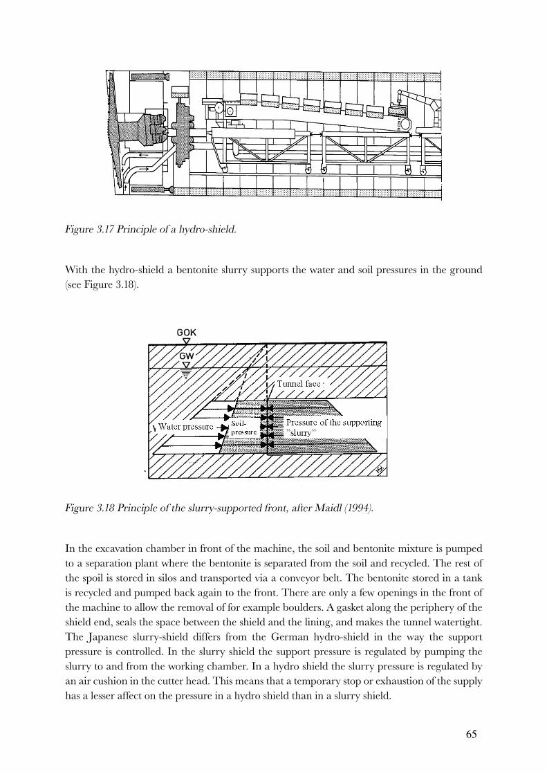
65

Figure 3.17 Principle of a hydro-shield.

With the hydro-shield a bentonite slurry supports the water and soil pressures in the ground (see Figure 3.18).

Figure 3.18 Principle of the slurry-supported front, after Maidl (1994).

In the excavation chamber in front of the machine, the soil and bentonite mixture is pumped to a separation plant where the bentonite is separated from the soil and recycled. The rest of the spoil is stored in silos and transported via a conveyor belt. The bentonite stored in a tank is recycled and pumped back again to the front. There are only a few openings in the front of the machine to allow the removal of for example boulders. A gasket along the periphery of the shield end, seals the space between the shield and the lining, and makes the tunnel watertight. The Japanese slurry-shield differs from the German hydro-shield in the way the support pressure is controlled. In the slurry shield the support pressure is regulated by pumping the slurry to and from the working chamber. In a hydro shield the slurry pressure is regulated by an air cushion in the cutter head. This means that a temporary stop or exhaustion of the supply has a lesser affect on the pressure in a hydro shield than in a slurry shield.

66

The combined shield is a shield with a slurry-supported front complemented with some additional equipment to increase its viable geological range. Furthermore, it is possible to rebuild the shield into another kind of front support, such as a mechanical shield. The hydro and slurry shields are used in sandy soils with low clay contents devoid of boulders. The combined shield was developed to use this kind of system in gravel containing boulders and clay. There are two different methods used to crush boulders in soil. Boulders can be crushed either by the cutters in the cutter head, or in a stone crusher located at the bottom or centre of the cutter head.

It is essential to achieve and maintain high water content in the soil, as clogging may occur when the clay in the soil is too dry. Clogging problems can be solved by:

− connecting a suction pipe to the excavation chamber, − introduction of a smooth wall into the excavation chamber, or − mounting the suction pipe on a moveable arm.

There is a pressure wall between the excavation and the pressure chambers. A double-gated chamber must first be traversed before entering the pressure chamber. The pressing block containing the stone crusher supports and drives the excavation ring.

Various mechanisms influence the stability of the face when hydro or slurry shields are used. The effects of several factors have been studied including: shear strength, consistence in soil conductivity, consistence and pressure in the slurry, penetration depth of the soil and the geometry (Anagnostou & Kovari,1994).

The geological conditions wherein shield machines fitted with slurry-supported fronts can be applied are characterised as sandy gravels containing water (see Figure 3.19). The support force is proportional to the diameter of the shield. In order to support the face, the pressure losses at the front caused by infiltration of the slurry into the ground have to be controlled. In order to avoid pressure losses in the face, the amount of fine grain (less than 0.02 mm) has to be about 10%. If the amount of fine grain is too high (>15-20%), clogging and increased separation problems may arise, as it is no longer possible to separate the fine grains from the bentonite (Barbendererde, 1991). In coarse-grained soils, fines in the slurry must be used to fill the pores. If these fine grains do not originate from the excavated soil, they must be introduced, for example by adding polymers.

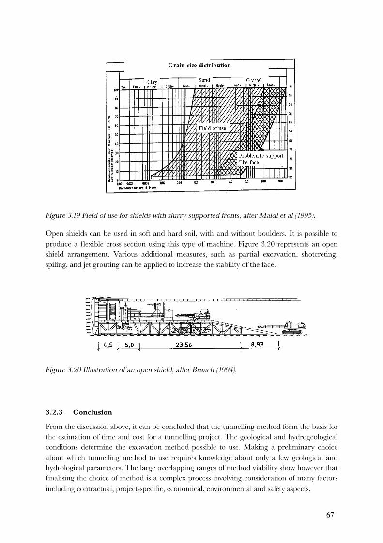
67

Figure 3.19 Field of use for shields with slurry-supported fronts, after Maidl et al (1995).

Open shields can be used in soft and hard soil, with and without boulders. It is possible to produce a flexible cross section using this type of machine. Figure 3.20 represents an open shield arrangement. Various additional measures, such as partial excavation, shotcreting, spiling, and jet grouting can be applied to increase the stability of the face.

Figure 3.20 Illustration of an open shield, after Braach (1994).

3.2.3 Conclusion

From the discussion above, it can be concluded that the tunnelling method form the basis for the estimation of time and cost for a tunnelling project. The geological and hydrogeological conditions determine the excavation method possible to use. Making a preliminary choice about which tunnelling method to use requires knowledge about only a few geological and hydrological parameters. The large overlapping ranges of method viability show however that finalising the choice of method is a complex process involving consideration of many factors including contractual, project-specific, economical, environmental and safety aspects.

68

Geotechnical characteristics affect the advance rate of the tunnelling method. Advance rates of different tunnelling methods in different geological conditions are discussed in the following section.

3.3 Geotechnical characteristics affecting the advance rate of tunnelling methods

3.3.1 Introduction

As discussed in Chapter 2, the time and cost for constructing a tunnel where no undesirable events occur, is called normal time and cost in the model. Normal time and cost can be expressed as a function of the advance rate. A number of factors affect the advance rate of tunnelling methods, including excavation equipment, the power source and transfer of reactive forces and the organisation (see Table 3.3).

Table 3.3 Factors affecting the advance rate, after Gehring (1995).

Rock Tool Equipment

Mechanical properties

Shape, size Size, weight

Petrographical properties

Material (s) Installed and transferable power

Rock mass properties

State of wear Transferable forces

Degree of alteration Load bearing capacity

Stability, stiffness

State of stress Array

Various examples of how different geotechnical characteristics affect the advance rate of tunnelling methods is discussed in the following section.

3.3.2 Examples using different tunnelling methods

Conventional method

Factors affecting the advance rate of conventional methods have been discussed in the literature by Purrer (1998). Besides geological conditions, there are also other factors that affect the advance rate. These include:

− the number of simultaneously excavated tunnel fronts (adits), − the number of and distance between the faces in partial excavation, − time losses due to the learning process at the start of a tunnel project, and − time losses associated with changes in the ground conditions.

With drill-and-blast methods, the time for drilling a round is affected by the brittleness, abrasiveness, strength and density of the rock. Clearly also machine-specific factors such as

69

the hammer geometry, velocity and frequency, as well as the design of the rods and bits all impact on the time required for drilling. A high degree of brittleness increases the penetration rate, while low abrasiveness decreases drilling time as bit-life increases and thus reduces the “downtime” spent on changes. Density only affects flushing.

The pie chart in Figure 3.21, represents the proportion of total work time allotted to different unit operations in an example of a conventional method. These data are from the South Marginal Zone in the Hallandsridge Tunnel, Sweden.

Figure 3.21 Proportion of total working time devoted to various unit operations using a

conventional tunnelling method (from the Hallandsridge Tunnel project).

Table 3.4 shows advance rates obtained from different projects using conventional methods in a range of geological conditions.

Table 3.4 Advance rates from projects using conventional methods, after Isaksson & Lindblad

(1997) and Sturk (1998).

Project Geology Area Advancement rate

Mean[m/month]

Advance rateMax

[m/month]

* Ayrton Senna Tunnel HeadingBenchHeadingBench

Sedimentary rockClay

Sand

52385238

11319260192

* Ilse tunnel Phyllite 8 200* Sieberg tunnelHeadingHeading

Miocene schlieren - sand, siltOligocene schlieren - sediment with clay

5252

180140

240180

* Hallandsridge TunnelFull faceHeading

Gneiss, Q=0.1-4Gneiss/clay/sediment, Q=0.005

33-4026

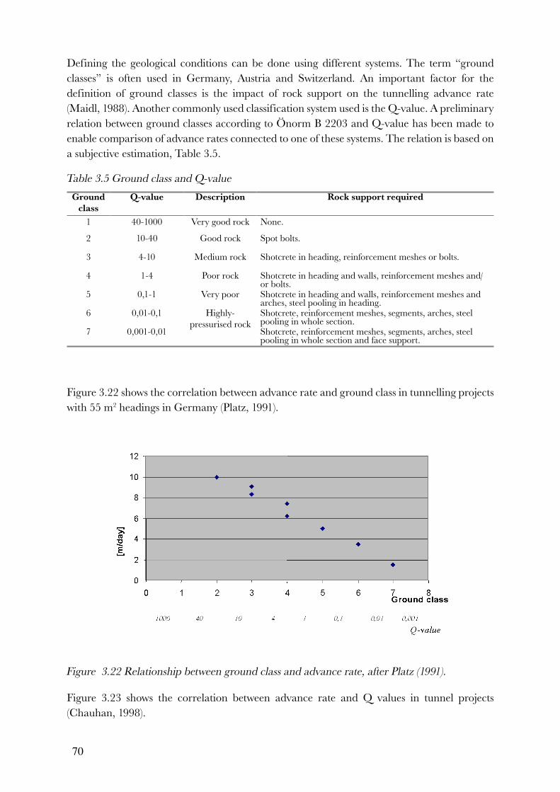
70

Defining the geological conditions can be done using different systems. The term “ground classes” is often used in Germany, Austria and Switzerland. An important factor for the definition of ground classes is the impact of rock support on the tunnelling advance rate (Maidl, 1988). Another commonly used classification system used is the Q-value. A preliminary relation between ground classes according to Önorm B 2203 and Q-value has been made to enable comparison of advance rates connected to one of these systems. The relation is based on a subjective estimation, Table 3.5.

Table 3.5 Ground class and Q-value

Ground

class

Q-value Description Rock support required

1 40-1000 Very good rock None.

2 10-40 Good rock Spot bolts.

3 4-10 Medium rock Shotcrete in heading, reinforcement meshes or bolts.

4 1-4 Poor rock Shotcrete in heading and walls, reinforcement meshes and/or bolts.

5 0,1-1 Very poor Shotcrete in heading and walls, reinforcement meshes and arches, steel pooling in heading.

6 0,01-0,1 Highly-pressurised rock

Shotcrete, reinforcement meshes, segments, arches, steel pooling in whole section.

7 0,001-0,01 Shotcrete, reinforcement meshes, segments, arches, steel pooling in whole section and face support.

Figure 3.22 shows the correlation between advance rate and ground class in tunnelling projects with 55 m2 headings in Germany (Platz, 1991).

Figure 3.22 Relationship between ground class and advance rate, after Platz (1991).

Figure 3.23 shows the correlation between advance rate and Q values in tunnel projects (Chauhan, 1998).

71

Figure 3.23 Relationship between Q values and advance rate, after Chauhan (1998).

Tunnelling machines

The influence that different geotechnical characteristics have on the advance rate of tunnelling machines has been described in the literature by Kuhnhenn (1995) and Bruland (1999) . Different parts of the construction process are affected by different geotechnical characteristics.

The following lists some of these factors by tunnelling phase.

− Excavation: granulometric composition, compactness, adhesiveness, and the presence of boulders.

− Support of the tunnel face: granulometric composition, compactness, adhesiveness, permeability, and soil stratification.

− Mucking out: granulometric composition, adhesiveness, cohesion, plasticity, and natural moisture content.

− Separation: granulometric composition, cohesion, and natural moisture content.

In order to obtain a high rate of advancement using shield machines, a number of factors interdependent on one other must be balanced. Tunnelling with a shield machine requires for example the following conditions:

− a stable and watertight front, − a good slurry/soil mixture, − constant support pressure, and − a muck-transportation drive system.

72

Some tunnelling methods require the geotechnical characteristics to fall within certain intervals in order to achieve high advance rates. An example of this relates to the content of fines in the soil, which must be above a threshold amount when using an open shield. In other tunnelling methods, increased levels of certain geotechnical characteristics may result in a decreased advance rate. An example of this when tunnelling with an EPB shield in soil containing boulders. Some tunnelling methods require the ground to exhibit specific levels of geotechnical characteristics in order to achieve high advance rates, above and below which the advance rate decreases. An example of this is tunnelling with a hydroshield, which is dependent on the content of fines in the soil.

Examples of the share of the total working time required for different unit operations using a combined shield are shown in Table 3.6. Here it can be seen that the tunnelling downtime using a combined shield with a slurry-supported face (Grauholz Zone 1) exceeds that of dry excavation in sandstone (Grauholz Zone 2). This provides an indication of the impact of complicated conditions on the advance rates.

Table 3.6 Time required for various unit operations as a share of the total tunnelling work

using a combined shield, after Aebersold (1994).

Project Geological conditions Boring

[%]

Ground

support by

segment

[%]

Downtime

miscellaneous

plus change of

cutters

[%]

Grauholz Zones 1 & 3

Moraine, boulders, water pressure

30 10 60

Grauholz Zone 2

Sand stone 50 10 40

Elbe (learning period)

Sand, clay, water pressure 18 30 52

City Express 26 20 54

Figure 3.24 shows the time required for various unit operations as a share of the total work time using tunnelling machines. These data were collected from the Grauholz Tunnel (Aebersold, 1994).

73

Figure 3.24 Share of the total work time required for various unit operations in tunnelling with

a combined shield. “Other” includes measures used in ground stabilisation to facilitate cutter

changes (from the Grauholz Tunnel project, after Aebersold, 1994).

Table 3.7 shows advance rates obtained with a TBM, and Table 3.8, advance rates using shield machines.

Table 3.7. Advance rates in TBM projects, after Gehring and Kogler (1997) and Aebersold

(1994).

Project Geology Diameter

[m]

Advance rate

Mean

[m/day]

Advance rate

Max

[m/day]

Evinos double shield open

Flysch, clay, boulders.Presence of methane gas.Limestone, sandstone, clay.Occurrence of radiolite.

4.0

4.2

26172010

Alpe Devero Lime shale, mica shale, dolomite, mica gneiss.Rock class 1-2.Rock class 2-3.

3.5

1823

31

Pradella-Martina Crystalline shale, amphibolite, gneiss. 5.5 23

Fernwärme München Sand/gravel below water level.New machine.Old machine.

5.010.78.7

Ilse Tunnel Phyllite crushed zone.Clay mylonite.

3.1 162.52

20

3Klösterle Phyllite gneiss, mica shale,

Crushed zone below water level.3.5 33

040

Basalt 85-190 Mpa, new machine.

Basalt blocksSand/siltstone 20-180 Mpa.

2223131827 35

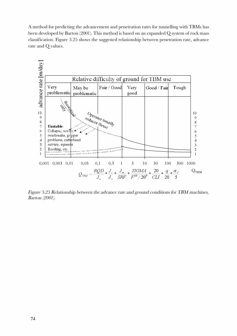
74

A method for predicting the advancement and penetration rates for tunnelling with TBMs has been developed by Barton (2001). This method is based on an expanded Q system of rock mass classification. Figure 3.25 shows the suggested relationship between penetration rate, advance rate and Q values.

Figure 3.25 Relationship between the advance rate and ground conditions for TBM machines,

Barton (2001).

75

Figure 3.26 shows a hypothetical comparison between the advance rates of methods using drilling-and-blasting and a TBM, (Barton, 2001). The dotted curves represent hypothetical monthly and yearly rates. From the figure it can be seen that the advance rate for the TBM and drill-and-blast methods are equally and strongly affected by the rock conditions. Drilling and blasting may prove very competitive to TBM if there are of either: (a) large cumulations faulted rock and poorer ground conditions, or (b) extensive, extremely good quality, massive rock. In areas where the rock quality lies somewhere in the range 0.1-10, the TBM would appear to be up to three times faster than drilling and blasting. It is important to note that the weekly advance rate cannot be extrapolated to a monthly or annual rate of progress. In long tunnels where there is statistically likely to be more extremes, drill-and-blast methods may exhibit superior performance than TBMs with respect to annual advance rate.

Figure 3.26 Hypothetical comparison of drill-and-blast and TBM advance rates in m/week

(solid curves). Dotted curves represent monthly and yearly rates, Barton (2001).

76

Table 3.8 Advance rates in shield projects, after Gehring and Kogler (1997) and Aebersold

(1994).

Project Geology Diameter

[m]

Advance

rate

Mean

[m/day]

Advance

rate

Max

[m/day]

Combined/hydroshieldGrauholz Zone 1 Moraine /boulders/ water pressure 3.7 bar. 11.8 4.5 8

Grauholz Zone 2 Sandstone. 11.8 17 24

Grauholz Zone 3 Moraine (boulders). 11.8 11 18

Elbe Filling sand - lose/hard. 14.2 6.6

Elbe Harder-packed sand. 14.2 7.6

Elbe Sand/boulders/water pressure 1.5 bar. 14.2 4.6

Metro Rome Sand, silt, clay. 6.6 12

Metro Rome Sand, silt, clay. 11 15.6

Metro Lyons D Sand, gravel, clay. 8.5 18

Metro Meteor Limestone, sand. 7.6 15

EOLE, Track 1 Limestone with sandy sections. 9 18

EOLE, Track 2 Limestone with sandy sections. 10 22

Villejust Sand. 14 36

Jubilee Line 105 Clay. 8 14.4

Jubilee Line 107 Sand, silt, clay. 8.4 19

EPB shield

Jubilee Line 110 Clay. 11 14.6

Metro Lisbon Clay, sand. 7 13

Metro Lille 1/3 Clay, limestone. 9 18.4

Open shield

Oued Sandstone - sand with clay. 10 4.0 5.4

From the above tables it can be concluded that high advance rates can be obtained when the tunnelling machine is selected and adapted to the prevailing geological conditions. Maximum advance rate is obtained when the machine is working under optimal conditions. Lower advance rates (as low as only a few metres per day) occur when the machines, for whatever the reason, cannot handle the prevailing geological conditions. It should be noted however that mean values for advance rates may also cover an initial learning period and include undesirable events encountered during the excavation.

3.3.3 Conclusion

Geotechnical characteristics affect the capacity of the tunnelling method. The advance rate for different tunnelling methods in a range of geological conditions has been described in the literature. It is important to consider the relationship between the tunnelling method’s advance rate and the geotechnical characteristics when estimating a project.

77

The various undesirable events that may impact on the tunnelling method are discussed in the following section.

3.4 Undesirable events affecting tunnelling methods

3.4.1 Introduction

As discussed in Chapter 2, undesirable events occasionally occur in tunnel projects due to various different factors, including geological or hydrogeological conditions. Some undesirable events occur rarely but lead to severe consequences, for instance where the geotechnical characteristics fall way outside the described range of normal application for the method, and the method has to be changed. Other undesirable events occur more often but lead to fewer consequences, for example rock falls.

A number of projects have been studied in order to obtain an overview of conceivable undesirable events and their cost consequences for tunnelling using conventional methods. This collection of project data has been carried out in a cooperative effort by Isaksson and Lindblad (1997) and Marxmeier (1997). Note that Tables 3.9 to 3.11 contain a range of symbols and abbreviations used in Tables 3.12 to 3.19 that follow.

Table3.9 Symbols used in Tables 3.12 – 3.19

Symbol Description

CS

Conventional method Shield machine

GMO

Event due to geological conditionsEvent related to mechanical failureOther undesirable event

BE

Event at the cutterheadEvent at the shield

FPY

Event at the face Event at the perimeterEvent at the surface

78

Table3.10. Combination of symbols used in Tables 3.12-3.19

Undesirable event Symbols Description

Events related to geological and hydrogeological

conditions using conventional method

At the face CGF1CGF2CGF3CGF4CGF5CGFY

Face collapseCollapse and water inflowCollapse at the benchCollapse due to deviation in bore inclinationWater inflowCollapse to the surface

At the perimeter CGP1CGP2

Collapse in the liningDeformations

At surface CGY1 Settlements

Miscellaneous

CO1 Execution failures

Events related to geological and hydrogeological

conditions using Tunnelling machines

At the face SGF1SGF2SGF3SGF4SGF5SGF6SGFY

Face collapseCollapse and water inflowJammingVertical deviation Water inflow No contact cutterhead-rockCollapse to the surface

At surface SGY1SGY2

Sink holeSettlements

Other SGO1 Methan gas

Function failure SGM1SGM2SGM3

Transport system not suitable for geological conditionsCutters not suitable for geological conditionsGrippers not suitable for geology

Problems at the perimeter

SGR1 Jamming of segments

Events related to machine and equipment

Cutter head SMB1SMB2

Main bearing failureScrew conveyor failure

Shield SME1SME2

Breake between head and tail Main component out of orderMiscellaneous

Material failure SO1SO2

HydraulicsVentilation fans

Table3.11 Description of consequence classes

Consequence

class

Description Cost

[% of tender price]

Example

I Minor consequences <10 Failure of segments.

II Medium consequences 10-50 Failure of main bearing.

III Major consequences 50-100 Face collapse.

IV Extreme consequences >100 Failure of the method.

Examples of undesirable events that may impact on projects where conventional methods and tunnelling machines are used are discussed in the following section.

79

3.4.2 Examples from different tunnelling methods


Various kinds of undesirable events that may occur using conventional methods have been discussed in the literature (HSE, 1996; Müller, 1978). Some examples of undesirable events related to geological and hydrogeological conditions are discussed in this section.

Undesirable events such as flooding or collapses may occur due to geological or hydrogeological conditions that impact on the method that go undetected by pre-investigations, for example:

− very hard rock, − very soft ground, − tectonic fault zones, − water-bearing caves, and − water-bearing sand or gravel.

Excavation using the drill-and-blast method under difficult conditions, for example with large cross sections in weak geological conditions such as in a fault zone, can be associated with the occurrence of extreme deformations that cause extensive damage to tunnel support. This occurred when benches of the two tubes were excavated for the 16-metre wide, three-lane Bolu Mountain Tunnel in Turkey (Brox & Hagedorn, 1999).

When a water-bearing zone is hit during excavation, the tunnel may become flooded. If the pumping capacity of the equipment is insufficient, excavation is interrupted and supplementary pump and drainage measures have to be taken. An example of this comes from a tunnel in Austria, where a water-bearing zone was hit at “normal” advance rate in a declining tunnelling drive. The tunnel was flooded and caused downtime running into several months due to the insufficient pumping capacity (Bauer, 1999; Diewald & Wolff, 1997).

According to HSE (1996), collapses occur principally:

− at the heading, − between the heading and the first completed section, and − where the lining is completed.

Where the overburden is thin, collapses in the heading may occur due to the unsupported section being too long. Additional reasons include the presence of excessive loose or weak rock mass that has not been bolted, or that the shear strength in water-filled ground is negligible, or even an application of an unsuitable design in the top heading invert. Collapse during excavation of the bench can occur due to missing bolts, or the distance between the front and the completed section being too long. Collapse during the installation of supporting structures may occur due to rotation of sidewall drifts, poor invert geometry, and high loading due to the amount of water in soft ground (thixotropic behaviour). Figures 3.27 and 3.28 show different types of collapse of the ground in the heading.

80

Figure 3.27 Ground collapse in the heading, HSE (1996).

81

Figure 3.28 Ground collapse in the heading, HSE (1996).

Collapse can also occur in the area of the tunnel heading between the excavated face and the first completed section, for example the collapse of unstable natural ground at the excavated face. If the primary lining is completed, a collapse can occur for example as a result of excessive settling or converge ce. Figure 3.29 shows various failures of the lining before closing of the section and Figure 3.30 shows various failures of the lining before or after closing of the section.

Figure 3.29 Failure of the lining prior to closing of the section, HSE (1996).

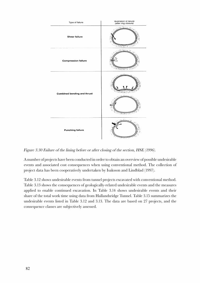
82

Figure 3.30 Failure of the lining before or after closing of the section, HSE (1996).

A number of projects have been conducted in order to obtain an overview of possible undesirable events and associated cost consequences when using conventional method. The collection of project data has been cooperatively undertaken by Isaksson and Lindblad (1997).

Table 3.12 shows undesirable events from tunnel projects excavated with conventional method. Table 3.13 shows the consequences of geologically-related undesirable events and the measures applied to enable continued excavation. In Table 3.14 shows undesirable events and their share of the total work time using data from Hallandsridge Tunnel. Table 3.15 summarizes the undesirable events listed in Table 3.12 and 3.13. The data are based on 27 projects, and the consequence classes are subjectively assessed.

83

Table 3.12 Undesirable events in tunnel projects using conventional excavation methods, to be

continued.

Project Year L

[m]

A

[m2]

Overburden[m]

Geology Cause Conse-quences[month]

Measures

Land-rücken Tunnel,Germany

1984 10779 150 Sandstone zone with clay, silt and sand.

CGF3 3.0 Additional anchors to prevent deformation. Grouting of collapsed material soft excavation.

Ayrton Senna Tunnel,Sao PauloBrazil

2000 75 Tertiary sediment rock, cohesion 150 kPa,friction angle 20°,clay/sand lenses.

CGF2

CGF3 0.5

New drainage system, grouting Shotcrete and grouting.

Undergr.MünchenGermany

1987 37-176

Hard layers of gravel and sand.

CGFYCGF2CGF4

Freezing of the crown Freezing.

Kavernen Garage,Lands-berg am LechGermany

182 mgarage,60 mtunnel

250 20 Sand and clay. CO1 Extra probe drilling and later change of position of the tunnel.

SchmittenTunnel,Zell am SeeAustria

1993 5837 0-200 Min.3.5

Weathered phyllite with high water content,Sandstone.

CGF1 Extra probe drill. Reduced round length, extra rock support.

Galgen-berg Tunnel,Austria

1994 5142 110-115

15-260 Lose layers of material, silt lenses.

CGY1CGF1CGY1CGP2

3.0Grouting, extra reinforcement,excavation with partial face.

Puymoren Pyrenees, France/Spain

4820 86 400-500 Granite, gneiss, shale, phyllite.

CGF3 More shotcrete and reinforcement, extra cautious excavation.

Sieberg Tunnel, Austria

1997 5008 115 0-50 Miocene and Oligocene schlieren.

CGF5 Reducedadvance-ment rate.

Pumps, draining ditches with stones and geotextile in the base.

Undergr.,Sao Paulo Brazil

1981 6 8 CGY1 Timber to prevent total collapse.

Santana Railway Tunnel, Brazil

1983 CGY1

Bochum Undergr., Germany

1984

1985

6.5 7.5 CGFYCGFY

Reduced distance between heading and bench.

Richthof-Tunnel Germany

1985 20 CGFYCGFY

3.0

Kaiserau-Tunnel, Germany

1985 25 CGF1 4.0 Excavation with side-wall drift.

Krieberg Tunnel, Germany

1986 3 km Sandstone CGF3CGY1

Weltkugel Tunnel, Germany

Be-fore1987

Sandstone CGF3

84

Table 3.12 continuation.

Project Year L

[m]

A

[m2]

Overburden[m]


Measures

Karawanken Tunnel,Austr/Slo.

1987

1989

Squeezing ground CGF2CGP1

Kehren-berg Tunnel, Germany

Be-fore1988

CGY1CGP2

Dewatering and ´side-wall drift´Timber propping.

Michels Tunnel, Germany

1988 CO1

Kwachon Tunnel, Korea

1991 15 Clay CGFY

Under-#1 gr., #2Seoul #3 Korea #4 #5 #6 #7

1991199119921993199319931993

28

Weathered rock and clay

Clay

CGFYCGFYCGFYCGFYCGFYCGY1CGY1

Damage toroads,supplymachine.

Lambach Road Tunnel, Austria

1992 CGFY

Chungho Road Tunnel, Taipei, Taiwan

1993 15 CGFY 24

Arienda, Santo Amaro, Sao Paulo, Brazil

Low over-burden

Fissured hard clay CGP2

Poggio Fornello, Toscana, Italy

1993 10.2 25 CGP2 Propping´ to prevent total collapse, 14 m long grouting bars in the face

Cardvalho Pinto Road Tunnel, Brazil

1994 CO1

Mont- #1mor #2Portugal

19941994

20 CGF1CGFY

Hallandsridge,Sweden

1991 16000 30-120

56 CGF1CO1

0.312

85

Table 3.13 Consequences of undesirable events occurred using conventional method and

measures used to enable continued excavation.

Undesirable event

Cause Consequences Measures

Collapse in the faceCGF1

• Poor geology and insufficient support of the face.

• Cracks due to excessive moments and forces.

• Downtime• Material

inflow

• Probe drillings• Reduced round length• Additionally rock support• Excavation with partial face• Stabilisation of the soil

Collapse and water inflowCGF2

• Failed soil stabilisation.

• Declined tunnelling.• Insufficient pumping

capacity.

• Inflow of material and water

• Flooding• Downtime• Settlements• Machine

damage

• Consolidation by jet grouting or freezing • Increase draining capacity. • Increase pumping capacity.• Timber

Collapse at the benchCGF3

• Overload of connection heading/bench

• Failure/insufficient support

• Long close of section

• Downtime• Material

inflow

• Cautious excavation• Grouting of collapsed material• Additional anchors

Water inflowCGF5

• Undetected waterzone/cave

• Insufficient grouting measures

• Flooding• Downtime• Machine

damage

• Pumping• Draining ditches

Collapse to the surfaceCGFY

• Fault zone• Prev. undiscovered

obstacles• Insufficient support

• Damage on buildings above

• Down time

• Support measures (freezing/jetgrouting)• Cautious excavation

Deformation at the perimeterCGP2

• Squeezing/swelling ground

• Insufficient support measuress

• Reduced cross section

• Damage on support/lining

• Extended cross section• Deformation joints in the shotcrete/lining• Extra support measures

SettlementsCGY1

• Loss of tension.• Insufficient support

measures.• Heterogeneous

geology.• Prev. undiscovered

obstacles.

• Deformation of lining.

• Damage to buildings above.

• Down time.

• Stabilisation of the soil. (Jetgrouting/freezing)• Checking of sensitive points.• Dewatering• Side wall drift• Long spiling• Reduced round length

Table 3.14 Time-related consequences in the South Marginal Zone (SMZ), Hallandsridge

Tunnel.

Description Share of the

total working

time [%]

Failure of equipment 0.3 - 2.6Failure of power or ventilation in the tunnel 0.4 - 1.3Geological investigation/information/media 0.3 - 7.1

86

Table 3.15 Summary of undesirable events listed in table 3.12.

Undesirable

event

Symbols Description Consequence

class

No.

Event related to geological conditions 42

Problems at the face.

CGF1CGF2CGF3CGF4CGF5CGFY

Face collapse.Collapse and water inflow.Collapse at the benchCollapse due to dev. In bore incl.Water inflow Collapse to the surface.

II-IIIII-IIIII-IIIIIII-IVII-III

5351114

Problems at the perimeter.

CGP1CGP2

Collapse in the liningDeformations

I-III-II

14

Problems at surface.

CGY1 Settlements I-III 8

Miscellaneous 4

. CO1 Execution failure II-IV 4

From the case studies it can be concluded that the majority of the undesirable events occurred due to geological problems at the face. Some undesirable events occurred in the tunnel lining, before the final rock support was done. Few undesirable events occurred due to unpredicted fault zones, which also led to major consequences. These might have been caused by inadequate pre-investigation, organization or checking systems. Undesirable events often cause downtime. After most undesirable events the excavation proceeded more carefully, with partial-face or sidewall techniques, and a faster closing of each section. In several cases an improvement of the ground was made by for example grouting, drainage and freezing. Additional rock support was often applied using for example anchors, shotcrete and more robust steel arches. In many cases an additional pre-investigation was also undertaken.

Tunnelling machines

Undesirable events that may occur when using tunnelling machines have been discussed in the literature by for example Aebersold (1994), Kovari (1985) and Wichmann & Isaksson (1997). Figure 3.31 illustrates some problems when tunnelling with TBM in poor rock.

Figure 3.31 Problems when tunnelling with a TBM in poor rock, where (a) unstable face, (b)

bore head stuck, and (c) reduction of cross section further back, Kovari (1985).

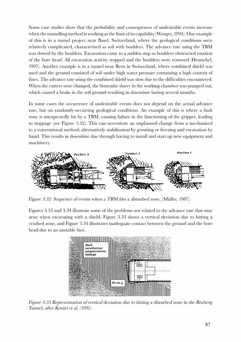
87

Some case studies show that the probability and consequences of undesirable events increase when the tunnelling method is working at the limit of its capability (Wenger, 1994). One example of this is in a tunnel project near Basel, Switzerland, where the geological conditions were relatively complicated, characterised as soil with boulders. The advance rate using the TBM was slowed by the boulders. Excavation came to a sudden stop as boulders obstructed rotation of the bore head. All excavation activity stopped and the boulders were removed (Hentschel, 1997). Another example is in a tunnel near Bern in Switzerland, where combined shield was used and the ground consisted of soil under high water pressure containing a high content of fines. The advance rate using the combined shield was slow due to the difficulties encountered. When the cutters were changed, the bentonite slurry in the working chamber was pumped out, which caused a brake in the soil ground resulting in downtime lasting several months.

In some cases the occurrence of undesirable events does not depend on the actual advance rate, but on randomly-occurring geological conditions. An example of this is where a fault zone is unexpectedly hit by a TBM, causing failure in the functioning of the gripper, leading to stoppage (see Figure 3.32). This can necessitate an unplanned change from a mechanised to a conventional method; alternatively stabilisation by grouting or freezing and excavation by hand. This results in downtime due through having to install and start up new equipment and machinery.

Figure 3.32 Sequence of events when a TBM hits a disturbed zone, (Müller, 1987).

Figures 3.33 and 3.34 illustrate some of the problems not related to the advance rate that may arise when excavating with a shield. Figure 3.33 shows a vertical deviation due to hitting a crushed zone, and Figure 3.34 illustrates inadequate contact between the ground and the bore head due to an unstable face.

Figure 3.33 Representation of vertical deviation due to hitting a disturbed zone in the Bözberg

Tunnel, after Kovári et al. (1991).

88

Figure 3.34 Representation of inadequate contact between the rock and the bore head due to

an unstable face in the Mont Russelin Tunnel, after Kavári et al. (1991).

When tunnelling through ground with a thin layer of overburden, settling may occur at the ground surface, which may cause major problems for existing buildings. Settling around the shield may occur due to for example compaction of the soil, and a higher concentration of spoil compared to undisturbed profile. An early and adequate grouting between the segment and the surrounding ground may reduce the amount of settling. Figure 3.35 shows how excess excavation has resulted in the formation of a sinkhole when tunnelling with a shield.

Figure 3.35 Sinkhole at the surface above the Grauholz Tunnel, after Steiner (1994).

Methane gas in the ground may cause an explosion in the tunnel. When tunnelling with a slurry-supported face, there is a minor risk of gas leakage, since methane gas can enter the tunnel through the slurry or gas-filled air pores in the spoil. There is a minor chance that the gas will explode in the shaft or pressure chamber using a slurry-supported face (Brasser, 1990). However, when using an open or an EPB shield, there can be a major risk of serious consequences in the event of a gas explosion.

89

Undesirable events may in some cases be related to the machine or equipment being used. Due to ever-rising wage costs, there is a corresponding increasing demand on the efficiency of tunnelling machines. A failure of a machine therefore has a major impact on the construction cost and time. According to Girmscheid (1997), Robbins (1982), and Maidl (1988), the failure of a machine can be caused by for example :

− the failure of a machine component, or − the inappropriate design of a machine component.

Upon the failure of a main machine component—for example a failure between the shield front and tail or failure of a screw conveyor—the excavation is interrupted and repairs have to be made. Experience from the Bötzberg and Zürichberg Tunnels, shows that downtime of several weeks resulted from main bearing failure in a shield/TBM (Kovari et al., 1991). Figure 3.36 shows repair work after failure of a main component in a shield machine.

Figure 3.36 Changing a main bearing from the surface above the Bötzberg Tunnel, after Kovári

et al. (1991).

In some cases gross operative errors occur (Wenger, 1994). These are usually characterised by major consequences and irregular occurrence. They arise mainly as a result of human error and are difficult to quantify and to totally avoid. It is a common mistake to spend time and resources on the analysis of the reliability of technical systems in spite of the fact that human errors and shortcomings contribute to the major part of the risk. The human factor is believed to be responsible for as much as 70-80% of all failures (Bartsch, 1995).

A number of projects have been conducted in order to obtain an overview of possible undesirable events and associated cost consequences when using tunnelling machines. The collection of project data has been cooperatively undertaken by Isaksson and Lindblad (1997), and Marxmeier (1998).

Table 3.16 shows undesirable events from tunnel projects excavated with tunnelling machines. Table 3.17 shows the consequences of geologically-related undesirable events and the measures applied to enable continued excavation. In Table 3.18 shows undesirable events and their share

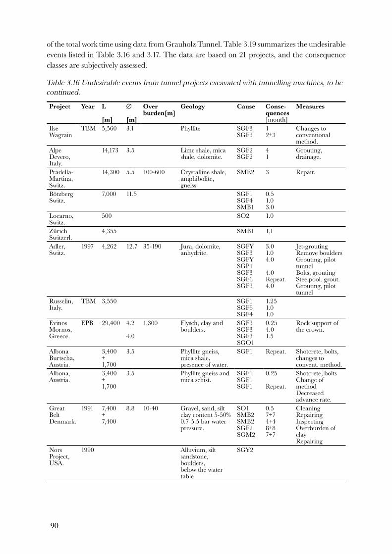
90

of the total work time using data from Grauholz Tunnel. Table 3.19 summarizes the undesirable events listed in Table 3.16 and 3.17. The data are based on 21 projects, and the consequence classes are subjectively assessed.

Table 3.16 Undesirable events from tunnel projects excavated with tunnelling machines, to be

continued.

Project Year L

[m]

∅

[m]

Overburden[m]


Measures

Ilse Wagrain

TBM 5,560 3.1 Phyllite SGF3SGF3

12+3

Changes to conventional method.

Alpe Devero,Italy.

14,173 3.5 Lime shale, mica shale, dolomite.

SGF2SGF2

41

Grouting,drainage.

Pradella-Martina,Switz.

14,300 5.5 100-600 Crystalline shale, amphibolite, gneiss.

SME2 3 Repair.

BötzbergSwitz.

7,000 11.5 SGF1SGF4SMB1

0.51.03.0

Locarno,Switz.

500 SO2 1.0

ZürichSwitzerl.

4,355 SMB1 1,1

Adler,Switz.

1997 4,262 12.7 35-190 Jura, dolomite, anhydrite.

SGFYSGF3SGFYSGP1SGF3SGF6SGF3

3.01.04.0

4.0Repeat.4.0

Jet-groutingRemove bouldersGrouting, pilot tunnelBolts, groutingSteelpool. grout.Grouting, pilot tunnel

Russelin,Italy.

TBM 3,550 SGF1SGF6SGF4

1.251.01.0

EvinosMornos,Greece.

EPB 29,400 4.2

4.0

1,300 Flysch, clay and boulders.

SGF3SGF3SGF3SGO1

0.254.01.5

Rock support of the crown.

AlbonaBurtscha,Austria.

3,400+1,700

3.5 Phyllite gneiss, mica shale, presence of water.

SGF1 Repeat. Shotcrete, bolts, changes to convent. method.

Albona,Austria.

3,400+1,700

3.5 Phyllite gneiss and mica schist.

SGF1SGF1SGF1

0.25

Repeat.

Shotcrete, boltsChange of methodDecreased advance rate.

Great BeltDenmark.

1991 7,400+7,400

8.8 10-40 Gravel, sand, siltclay content 5-50%0.7-5.5 bar water pressure.

SO1SMB2SMB2SGF2SGM2

0.57+74+48+87+7

CleaningRepairingInspectingOverburden of clayRepairing

Nors Project,USA.

1990 Alluvium, silt sandstone, boulders,below the water table

SGY2

91

Table 3.16 continuation

Project Year L

[m]

∅

[m]

Overburden[m]


Measures

Meidrich,Germany.

3,600 10-25 Gravel, sand, clay, bouldersfill quant., below the water table.

SGY2SGM1

Rebuilding the machine.

Grauholz,Switz.

1993 5,550 11.6 8-120 Sandstone, clayey-moraine, boulders.

SGF1SGF1SGY1

62

FreezingJet-grouting

Elbe,Hamburg,Germany.

1999 2,600 14.2 7-13 Sand, gravel, boulders, mica shale.

SGF5SGF3SMB3

0.42.52.0

Add. groutingRepairingrepairing

DB zent.,Germany.

SGF2 3.0

Fernwe.München,Germany.

6,000 5.1 Sand, gravelbelow the water table

SGF4SME2SME1

0.70.20.1 Repairing

NorsProject,USA.

1990 5.2 20 Silty-sand SME2SGY1 Repeat.

Adv.ratdecr.

RepairGroutingSuppl. of machine

HallandsåsSweden.

1991- 17,000 30-120

4.55 Gneiss, amphibolite.

SGM3 12 Change of tunnelling method

OuedOuchaia,Algeria.

920+960

10 0-26 Sandstone, layer of lime stone, clayey-sand, high percentage of water.

SGF1SGF1SGM2

0.10.1Repeat.

GroutingFilling of cavityChange of equipment to hydraulic hammer

92

Table 3.17 Consequences of geology-related undesirable events occurred using tunnelling

machines and measures applied to continue with the excavation, to be continued.

Un-

desirable

event


Collapse in the faceSGF1

• Emptying of slurry• Little overburden• Poor cohesion in soil

layers• Loss of pressure

• Work under excess pressure

• Downtime

• Minimise the frequency and time for work under excess pressure, e.g. by optimising cutter changes.

• Facilitate closing the bore head.• Create durable skin at the face.• Increase the rock support.

Collapse and water inflowSGF2

• Absence of waterproof joint.

• Incorrect grouting substance.

• Failure in joint.• Failing stabilisation of

soil.• Declining tunnelling.• Insufficient pumping

capacity.

• Loss of pressure

• Collapse• Flooding• Downtime• Settlements• Machinery

damage

• Consolidation by jet-grouting or freezing l• Increase draining possibilities. • Increase pumping capacity.

JammingSGF3

• Slow advance rate.• Swelling ground.• Incorrect steering

system.• Compression strength

of the soil so low that the machine sinks.

• Deformation of segment.

• Down time.

• Facilitate withdrawing the gauge cutters• Facilitate increasing the advance rate.• Flexible segment system.• Support of the soil with rock.• Select reliable steering system.• Additive reducing friction between rock and

shield.• Suitable machine design.

High wear on the mucking- system

SGM1

• High abrasiveness of the excavation quantities.

• Lengthy downtime for repairs.

• Change design of the slurry pumps.• Use flexible conveyor.• Treat the curved pipes for the slurry.• Adequate spare-parts storage.• Regular checking.

Stoppage in the slurry-supply systemSGM1

• Power-supply stoppage.

• Wear and tear.• Valve failure.• Compressor stoppage.• Pressure increase in

the pipes.

• Pressure loss• Collapse

• Reserve valves in the passages.• Reserve compressors.• Reserve power supply and delivery.

Stop in the separating plantSGM1

• Sticking • Closing down the site.

• Wear of hydrocyclone

• Facilitate developing the separation process.• Repair

Problems with cuttersSGM2

• Insufficient penetration.

• Poor geological prognoses.

• Insufficient resistance of the segment

• Downtime • Vary the speed of rotation of the bore head.• Facilitate drawing the bore head back.• Prepare the face for different kinds of bore

equipment.

93


Un-

desirable

event


The bore head sticks.SGF3

• High clay content. • Reduced advance rate.

• Downtime.

• Rotation of the bore head in different directions.

• Separate adjustable centre head.• Rinsing jet in the lower part of the bore head

in the crusher and in the openings.• Equipment for rinsing of the head.• Facilitate vibration.• No vertical bore head.

SettlementsSGY2

• Loss of tension.• Excessive soil outlet.• Vibrations.• Insufficient ring bogus• Heterogen. geology.• Insufficient support

pressure.• Unexpected obstacles.

• Deformation of segment.

• Damage to buildings above the site.

• Stoppage.

• Early and sufficient grouting of the ring column.

• Suitable shield end tightening.• Facilitating closing the face.• Checking the support pressure.• Stabilising the soil.• Rapid addition of fresh bentonite.• Checking sensitive points.• Checking the groundwater level.

Table 3.18 Undesirable events and their share of the total working time, using data from the

Grauholz Tunnel.

Undesirable event Percentage of total working

time [%]

Undesirable event Percentage of total

working time [%]

Miscellaneous (failure in) Machine failure

Reinforcement Hydraulics 1.5

Power in the tunnel 0.1 Crusher 0.5

Hydraulics 1.5 Motors 0.3

Power in the shield 0.1 Grippers 0.3

Grippers 0.4 Water proofing 1.8

Compressor 0.2 Compressor 0.1

Vacuum arm 0.8 Jet piping 0.1

Engines 0.2 Passing 0.1

Ventilation 0.2 Sticking 1.7

Grouting pump 0.4 Boring

Various stoppages Power in the tunnel 0.2

Changing pipes 0.4 Greasing 0.1

Geological investigations 0.7 Bentonite 3.9

Cleaning 3.3 Power in the shield 0.1

Face collapse 3.5 Water supply 0.1

Repairing 2.6 Ventilation 0.1

Remaining 1.3 Compressor 0.1

Material support Total machine failure

11.0

Conveyer belt 0.4 Primary separation

Crane 0.1 Piping 0.6

94


Undesirable event Percentage of total working

time [%]

Undesirable event Percentage of total

working time [%]

Change of cutters Layer 1.6

Tapping/filling of bentonite 1.4 Pumps 0.8

Unplanned changes in the face 0.4 Unloading station 0.1

Total miscellaneous 18.0 Mud container full 0.4

Power 0.4

Piping system Overrun 0.5

Stoppage in the piping 2.3 Secondary separation

Extractors 0.2 Pump 0.4

Secondary piping 0.5 Bentonite 0.2

Pumps 0.2 Band presser 0.2

Leakage in the piping 0.8 Centrifuge 0.2

Total piping system 4.0 Mud container full 2.3

Power fault 0.2

Water supply 0.1

Total separation 8.0

Table 3.19 Summary of undesirable events listed in Tables 3.16.

Type ofUndesirable event

Symbols Description Consequence

class

No.

Events related to geological conditions 41

Problems at the face.

SGF1SGFYSGF2SGF3SGF4SGF5SGF6

Face collapse.Collapse to the surface.Collapse and water inflow.Jamming.Vertical deviation.Water inflowNo contact between cutter head and rock.

II-IIIII-IIIIIIIIIIII-IIIII

10249312

Other SGO1 Methane gas leak II-III 1

Functionfailure(TBM).

SGM1SGM2SGM3

Transp. system unsuitable for the geology.Cutters unsuitable for the geology.Grippers unsuitable for the geology.

II-IIIII-IIIIV

121

Problems at the perimeter.

SGP1 Jamming of segments. I 1

Problems at the surface.

SGY1SGY2

Sink hole.Settlements.

II-III

22

Events related to mechanical failure 8

Cutter head. SMB1SMB2

Main bearing failure. Screw conveyor failure.

III

22

Shield break. SME1SME2

Head / tail.Main component out of order.

III

13

Miscellaneous 2

Material failure.

SO1SO2

Hydraulics.Ventilation fans.

II

11

From the case studies investigated, it can be concluded that most of the undesirable events that occurred were connected with the geological conditions. Many of the undesirable events

95

occurred due to unexpected geological conditions, such as clay, boulders and weathered rock. The problems often occur at the face. After collapse with a TBM, filling of the cavity was often undertaken. Continuing on with excavation required the reinforcement of the ground with for example anchors, grouting or freezing. Some undesirable events were related to machine and equipment. Naturally enough these problems were often followed up by repair work. In some cases the excavation method itself was changed. In one case (a fault zone containing clay and water) a change to the conventional excavation method was deemed necessary.

3.4.3 Conclusions

All the case studies investigated illustrate that different types of undesirable events do occasionally occur and cause a range of consequences for the respective project in terms of time and cost. Some of the events that occurred depended on the actual capacity of the method, others occurred randomly due to the geological and hydrogeological conditions encountered along the way. There are other events that occurred due to failure of machinery or equipment. Gross human errors have also caused undesirable events. It is important to consider the affect of undesirable events on the total time and cost in the estimation.

To describe the flexibility and preparedness to meet actual conditions of a tunnelling method the term robustness is used. How the robustness of a method influences the advance rate of tunnelling machines is discussed in the section that follows.

3.5 Measures for increasing robustness

3.5.1 Robustness and the tunnelling method

It is important that the tunnelling process is robust. Robustness in this context means tolerant or flexible to variations in potentially-disruptive factors. A tunnelling method is considered robust with respect to a certain geotechnical characteristic, when variations in the magnitude of that characteristic only lead to minor detrimental affects on the capacity of the method. Increasing the robustness of the tunnelling method often results in increasing its capacity or geological range of application or both, and reducing the probability and the consequences of undesirable events. Development of robust methods may raise the cost of the method, but often reduce the total time and cost for the project as a whole. In the manufacturing industry, different methods have been used to estimate robustness (Taguchi, 1993).

Robustness-increasing measures can be applied to technical as well as non-technical parts of the process such as contracting and management. These measures can be applied during different phases of the process, for example during the tendering phase or the construction phase.

96

Various measures used to improve identification and control of risks have been discussed in the literature (HSE (1996), including introducing:

− an international database of undesirable event reports, − guidelines for measures to be used in the planning stage, − risk-reducing measures in tunnel contracts, − increased co-ordination, co-operation and communication at the site, and

− an international database containing the best practical solutions for reducing risks and increasing control.

It is important to decide as early as possible in the planning stage which measures are to be used to increase robustness, as it often is more expensive and more difficult to integrate these later on in the construction phase (Rausand, 1991).

Measures that can be applied in the planning stage are for example:

− pre-investigations, − quality control, − staff training, − design optimisation, − adequate preparation for the spare equipment needed, − suitable risk-sharing between the parties, and − realistic time scheduling.

The value of pre-investigations of the geology has been discussed in the literature by for example Olsson and Stille (1980), and Einstein et al. (1991). In this respect, using a shield machine, where the choice of available measures such as separation plants and boulder crushing strongly depends on the actual geological conditions encountered, may require better knowledge about the geological conditions than using a drill-and-blast method, which is more flexible and facilitates direct access to the tunnel face.

When the overburden is expected to be considerable, one alternative to expensive core-drilling from the surface can be to excavate a pilot tunnel first.

Quality control has been discussed in the literature by Stille et al. (1998). The risk of personnel-related mistakes occurring could be decreased through personnel training (Rausand, 1991). It is important to plan for a working organisation that can identify and prevent undesirable events. Undertaking risk analysis before the construction work starts shows that material-related hazards can be prevented (Chiaverio et al., 1995).

Various different measures can be applied during the construction phase. The correct measures for using with each tunnelling method depend on various factors. For example, knowledge about what technical solutions are available and appropriate, and the actual ground conditions encountered affect the ability to choose suitable measures. Measures for increasing the method’s robustness can be applied in the following areas:

− the shape and cross section of the tunnel, − improving the condition of the ground,

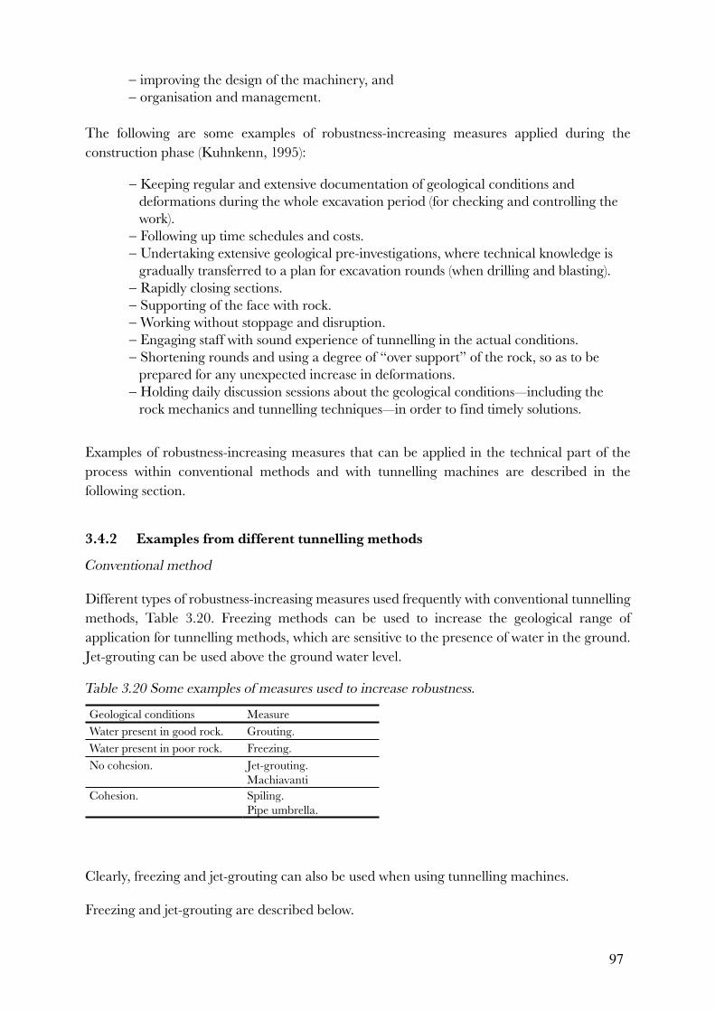
97

− improving the design of the machinery, and − organisation and management.

The following are some examples of robustness-increasing measures applied during the construction phase (Kuhnkenn, 1995):

− Keeping regular and extensive documentation of geological conditions and deformations during the whole excavation period (for checking and controlling the work).

− Following up time schedules and costs. − Undertaking extensive geological pre-investigations, where technical knowledge is

gradually transferred to a plan for excavation rounds (when drilling and blasting).− Rapidly closing sections.− Supporting of the face with rock.− Working without stoppage and disruption.− Engaging staff with sound experience of tunnelling in the actual conditions.− Shortening rounds and using a degree of “over support” of the rock, so as to be

prepared for any unexpected increase in deformations.− Holding daily discussion sessions about the geological conditions—including the

rock mechanics and tunnelling techniques—in order to find timely solutions.

Examples of robustness-increasing measures that can be applied in the technical part of the process within conventional methods and with tunnelling machines are described in the following section.

3.4.2 Examples from different tunnelling methods

Conventional method

Different types of robustness-increasing measures used frequently with conventional tunnelling methods, Table 3.20. Freezing methods can be used to increase the geological range of application for tunnelling methods, which are sensitive to the presence of water in the ground. Jet-grouting can be used above the ground water level.

Table 3.20 Some examples of measures used to increase robustness.

Geological conditions Measure

Water present in good rock. Grouting.

Water present in poor rock. Freezing.

No cohesion. Jet-grouting.Machiavanti

Cohesion. Spiling.Pipe umbrella.

Clearly, freezing and jet-grouting can also be used when using tunnelling machines.

Freezing and jet-grouting are described below.

98

By freezing the ground, any water present in it is converted to ice. The frozen ground has almost the same strength as shotcrete, it can form a waterproof barrier and is chemically neutral. Freezing has almost no influence on the surrounding groundwater. The mechanical and thermal parameters of the soil must be known in order to obtain an appropriate construction. The tensile strength of the frozen ground depends on the quality of the ice, and the uniaxial compressive strength of the grain size distribution.

Freezing can be achieved independently of the excavation process, for example when undertaken from a tunnel above the excavation area or from the surface when the overburden layer is thin. However a more exact profile can be achieved when freezing from the tunnel face (see Figure 3.37). The volume of soil necessary to freeze is also less than when freezing from the surface. This reduces the cost. However there will be some downtime using this method as the excavation is interrupted. When two parallel tunnels are excavated it is possible to alternate between freezing and excavating activities.

Figure 3.37 Representation of the principle of horizontal freezing, after Maidl (1988).

Brine or liquid nitrogen can be used as freezing media. The medium circulates through a freezer system at temperatures of below -30˚C (brine) and –196˚C (nitrogen). After circulation, the cooled nitrogen is emitted into the air at a temperature of approximately –60˚C.

Advantages using liquid nitrogen as a freezing medium include for example:

− lower costs for site mobilisation, − short freezing times, − is taste and odour free, − is non-combustible, − is non-toxic, − is effective when the groundwater flow is relatively high,

99

− does not require any temporary storage, as the gas supplier usually provides all the necessary application equipment including tank, flow gauges, hoses and applicators.

One disadvantage with liquid nitrogen is the risk of suffocation of workers should leakage occur in confined spaces.

As a freezing medium, brine is less expensive than liquid nitrogen when trying to achieve longer freezing times and larger volumes of frozen ground. In order to freeze the ground, the water content in the soil must be at least 5-7%, and the groundwater flow velocity a maximum of 1-3 m/day. It may be necessary to also incorporate a grouting umbrella or to reduce the distance between the freezer pipes to reduce the groundwater flow. To increase the water content in the soil, it may be necessary to add water. If water has not been sucked up from the surroundings, the soil consistence will after thawing, be the same as before the freezing process. Damage from freezing and thawing only occurs in compact soils with slow or repeated freezing, or a combination of both. According to Maidl (1988), some of the disadvantages of using brine compared with using liquid nitrogen are for example:

− the high cost for site mobilisation,− high demand for bore accuracy (normally a tolerance of less than 1% of the inclination

of the length of the bore), and where major deviations can increase the time required to achieve a homogeneously frozen ground, and

− leakage of the cooling medium into the ground often results in lowering the freezing temperature.

Jet-grouting can be used to increase the geological range of application in the soil above the groundwater level. Contrary to normal grouting (which can only be used in coarse-grained soils) and chemical grouting (which can only be used in soils with permeability (k) of between 10 -2 to 10 -4 cm/s), jet-grouting can be used in soils defined as fines (Figure 3.38).

Figure 3.38 Range of application for jet-grouting, after Maidl (1988).

100

Jet-grouting changes the soil structure, as piles are produced, consisting of a mixture of soil and added cement (grout). Cement, water and air are added from separately located pipe jets—one, two or three-phase bars. In a single-phase system, only the cement is added. In a two-phase system, cement and air are added, and in a three-phase system, cement, water and air are added to the soil under high pressure (Martak, 1986; Arz et al.,1991). The cross section, strength and permeability of the grouted pile depend for example on the geological conditions, the pump pressure, the mixture used, the rotational speed of the drilling bar as well as the pull-back speed of the bar. The slurry back flow can be used to control the size of the piles. It is very difficult to determine the exact content of the cement in the slurry back flow. The discharge of material during drilling can be reduced when the time elapsing between drilling and grouting is reduced. It is important to construct test piles, as the geological conditions impact on the characteristic of the pile. The same equipment for the actual drilling process should be used when constructing the test piles. The compressive strength varies between 10-18 MPa depending on the geological conditions. Table 3.21 shows parameters for various systems.

Table 3.21 Parameters for various systems.

Parameter Unit Single-phase

system

Two-phase

system

Three-phase

system

WZ-value 0.8-1.0 0.8-1.0 0.7-1.0

Water pressure [bar] - - 300-600

Pile diameter [m] 0.35-1.0 0.5-1.6 0.8-2.5

Air pressure [bar] - 7-14 7-14

Cement pressure [bar] 300-600 300-600 5-80

Jet-grouting is used not only for reinforcing the soil, for instance under foundations or inverts, but also for temporary support prior to constructing more long-term rock support for preventing settling and increasing the stability of faces. If the grouting is performed below the groundwater level, the water must be checked with regard to chloride corrosion and the appropriate measures taken to prevent the circulation of groundwater should it be deemed necessary. The pile sections can be made in an overlapping way—one after the another—or in intervals. For example in sand and soil containing boulders, some five to six piles, each with a length of 17 m can be completed each day. Deviation should not exceed 1° for each 15 m length of drilling. For longer drilling, the deviation should not exceed 2.5°.

The following are some of the advantages of jet-grouting.

− It is versatile and can be used in a range of different tunnel profiles. − It provides a good basis for future rock support by shotcrete. − It increases the stability of the face. − It increases the level of safety for the tunnel workers. − It reduces the need for other temporary reinforcement measures. − It is profitable in short tunnel sections. − It facilitates continuous information flow about future tunnel sections. − It reduces settling by up to 50-60% compared with pilot tunnelling. − It is adaptable to changing ground conditions. − Boulders in the soil can be integrated precisely into the construction work

101

− The number of piles can be increased or reduced in accordance with the geological conditions encountered.

The following are some of the disadvantages of jet-grouting.

− Estimating the diameter of the piles is almost impossible without conducting tests. − Low tolerance of drill deviations where piles perform a tightening function.− Leakage is almost impossible to localise and therefore cannot be treated.− Under conditions of high water pressure and fine-grained soil, even a small hole in

the umbrella allows soil to flow into the tunnel and cause problems. − When the ground contains water, several layers of piles may be required. − In hard packed moraine, the pile diameter is often overestimated, especially when

using two-phase systems. − Careful pre-investigation is necessary when the construction must be watertight.

Tunnelling machines

Various types of measures can be applied for increasing the robustness of different tunnelling machines (see Table 3.22).

Table 3.22 Examples of measures to increase robustness in tunnelling machines, after Maidl et

al. (1995) and Girmscheid (1997).

Shield machine Geological conditions Measures

Combined/slurry Occurrence of bouldersHigh content of fines

Low content of fines

Integrate stone crusher Strong separation plant/separate centre cutter/foam/flush holes/larger centre holes in cutter head.Additive

EPB High permeability Add foam.

Open Low cohesion Jetgrouting

In order to expand the geological range of application of combined-shield machines, various substances can be added to the slurry. In order to reduce “pressure loss” when excavating with an EPB shield in large-grain-size soils with low fine contents, a mixture of bentonite, polymers and filling material can be added to the excavated material (Maidl, 1995). Figure 3.39 shows how the addition of sawdust increases the sealing capacity of the material.

Figure 3.39 Grain distribution when sawdust is added, after Steiner (1993).

102

In swelling ground, the design of the machine and the lining ought to be taken into consideration and improvements made. The ground should be allowed to move in the joint zones, which reduces the tension in the lining. It is advantageous to have a short machine and even to modify the shape of the cross section. Increased advance rate, and counteracting pressure reduces the deformation of the lining. A slow advance rate is required to avoid getting the machine stuck. Slow advance rate in response to swelling leads to the need for increased support measures, which further slows the advance rate. Using a TBM improves access to the bore head. Increased support does not impact on the advance rate as much as for example using a shield machine. However should the machine get stuck, major efforts would then be required to release the machine. Figure 3.40 represents the correlation between time required for rock supporting measures and the advance rate required.

Figure 3.40 Illustration of the correlation between the time required for rock support and the

advance rate required for shield and TBMs, after Vigl and Jäger (1997).

One measure that reduces the probability and consequences of undesirable events when using tunnelling machines is using a geophysical pre-investigation system. One such system is integrated into the bore head and based on acoustic reflection measurements. The Sonic Soft Ground Probing System (SSP method) has been developed especially for continuously checking the geology in front of the tunnel face (see Figure 3.41). The position of for example boulders and other obstacles, sloping/vertical or coarse-layer limits, or water-bearing sand lenses in clay can all be fixed with this system (Girmscheid, 1997). With this system the tunnel workers are able to take preventative measures in time to reduce risks that would lead to downtime for repairs or rock support.

103

Figure 3.41 Seismic measuring equipment integrated into the bore head, after Sonic Soft

Ground Probing (1995).

Another system used for geophysical pre-investigation has been developed in Japan. This system uses a combination of acoustic and Rayleigh waves. This combination enables the prediction of the geological conditions up to 10 m in front of the face. However this system has only been applied in a limited number of projects (Kasa et al. 1994).

3.5.3 Concluding comments on increasing robustness

From the above it can be concluded that robustness-increasing measures can be used to increase the geological range of application and the advance rate of a tunnelling method. These can also reduce the probability and consequences of undesirable events. The measures that are most suitable depend on the tunnelling method used. The effects of measures used to increase robustness ought to be considered when estimating the time and cost for the tunnel project.

3.6 Conclusions

The tunnelling method and the geotechnical characteristics are the basis of estimating time and cost for a tunnel project.

The geological and hydrogeological conditions determine the best tunnelling method to use. Relatively few geological and hydrological parameters are required to make a preliminary choice. The large overlapping ranges of method viability shows however, that the final choice of method is a complex process, where contractual and project-specific factors as well as economical, environmental and safety aspects all have to be considered.

Geotechnical characteristics also affect the productivity of the tunnelling method. In the literature the advance rates of different tunnelling methods in a range of different geological conditions have been described. It is important that the correlation between the advance rate of the tunnelling method and the geotechnical characteristics are taken into account in the estimation model.

104

All the case studies show that different types of undesirable events do occasionally occur, and have consequences for each respective project in terms of time and cost. Some of the events that occur depend on the actual capacity of the method, others occur randomly due to the geological conditions encountered. There are also events that occur due to failure of machinery or equipment. Gross errors are also the cause of some undesirable events. It is important to consider the impact on time and cost due to undesirable events.

It has been concluded that robustness-increasing measures can be used to increase the geological range of application and the advance rate of the method. These can also reduce the probability and the consequences of undesirable events. The most suitable measures depend on the tunnelling method used. The affect that robustness-increasing measures have on time and cost should be considered when estimating time and cost for a tunnel project.

The next chapter presents a detailed structure for an estimation model for tunnelling projects, which takes into consideration the requirements discussed here.

105

4 Modelling of time and cost

4.1 Introduction

In Chapter 2 the demands placed on an estimation model of time and cost for tunnelling projects have been discussed. Based on this discussion, it has been concluded that it is important that the client and the contractor have a sound basis for making decisions about budget and tender pricing. Both parties need to base their decisions on a statistical distribution of total time and cost. Furthermore, the construction-contracting method itself, as well as each stage of the project affect which particular party—the client or the contractor—is responsible for the increases in time and cost that may occur due to different risk factors. Different risk factors should therefore be able to be considered in the basis for decision-making.

Two important factors in the estimation of time and cost are the tunnelling method and the geotechnical characteristics. Different tunnelling methods are affected by different risk factors. As discussed in Chapter 3, different measures for increasing robustness can be applied to the methods in order to reduce the probability and consequences of undesirable events and increase the capacity of the method. Geotechnical characteristics affecting the geological range of the method and the capacity of the method are important factors that should be considered in the estimation model.

As discussed in Chapter 2, the tunnelling process can be seen as a “series” system, where the main activities lie along a critical time path. During the estimation of the total time required for the project, only the critical activities need to be considered.

As with all modelling, it is important to realize that this model as all models is just a representation of reality, with the purpose of providing an efficient tool for assisting decision-making.

This chapter provides both the theoretical background to an estimation model as well as some practical applications. The principles for the estimation of time and cost are discussed, as well as how to obtain the input data required for the model.

4.2 A theoretical estimation model

4.2.1 Expressing parameters

As in all other geotechnically-based problems, many of the parameters must be expressed as stochastic variables. The total time or cost can therefore be expressed as a function of several variables, both deterministic (a

i), and stochastic (b

i):

(4.1)

Some of the variables in the function are correlated; consequently there is a need for handling this in the estimation of total time and cost.

As discussed in Chapter 2, there is normal time and cost, and there is exceptional time and cost. The total time or cost (C) for a project can in principle be expressed as the sum of the normal

106

time or cost (Cn) and the exceptional time or cost (C

e):

(4.2)

As discussed in Chapter 2, the definition of undesirable events and normal time is subjective, which can clearly be seen from the definition of an undesirable event being, “a factor that causes major unplanned changes in the tunnelling process”.

As discussed in Chapter 3, the term advance rate is used to express the capacity of a tunnelling method as, “the length of excavated tunnel per unit time” (for example m/day). However in the estimation model, the inverse of the advance rate—the time consumption for excavating a tunnel unit using a certain tunnelling method” (for example in h/m)—is used to facilitate the mathematical calculation. The term used for this inverse in this study is the production effort. Other examples of the production effort are the quantities that have to be carried out per tunnel unit, e.g. the amount of shotcrete.

Estimation of normal time and cost as well as exceptional time and cost is discussed in this chapter.

4.2.2 Normal time and cost

The time and cost for constructing a tunnel, provided no undesirable events occur, is called normal time and cost in this model. The normal time and cost can be expressed as a function of the production efforts of the method i.e. the work to carry out or handle a tunnel unit. Under a normal time-and-cost regime, a tunnel unit is a “unit length”, and in the case of an undesirable event, “the complete handling of the consequences of the undesirable event”.

For estimation of the time, the production efforts is the effort expressed in working hours per unit length for the activities lying on the critical path. For calculation of the cost, different types of production efforts has to be considered like the quantities to be carried out per tunnel unit as well as working hours per unit length, see chapter 4.3.3.

The production effort of a tunnelling method depends on the geotechnical characteristics. As knowledge about the geotechnical characteristics is limited, due to the limited number of samples (Salazar, 1985), these are best expressed as stochastic variables. Even if one in principle can find a deterministic relationship between the production effort and the geotechnical characteristics, it has to be regarded as stochastic variable. Figure 4.1 presents an example of the relation between a single geotechnical characteristic and the production effort.

107

Figure 4.1 Example of the correlation between production effort (y) and a geotechnical

characteristic (x).

The geotechnical characteristics tend to vary from one point to another. The method specific production effort in each point in the tunnel depends on the geotechnical characteristic, expressed as x(l), with a given distribution, f

x(x). The relationship between the characteristic

and the production effort can be expressed as a stochastic function, g(x(l)). When estimating the normal time and cost it is necessary to consider the production effort (Q) for the studied tunnel length. It is important to realize that the production effort for the studied tunnel length is also to be regarded as a stochastic variable. An estimation of production effort in a certain length interval can be made. It is assumed that the characteristics in each point in the studied tunnel length are uniformly distributed but not necessarily uncorrelated. This results in a uniformly-distributed production effort in each point in the studied tunnel length (but not with the same distribution as the one for the geotechnical characteristics).

The expectation E(y) and standard deviation σy of the production effort y=g(x), can in principle

be estimated from the following equation (after Benjamin & Cornell, 1970):

(4.3)

and

(4.4)

and the probability density function, as:

(4.5)

The production effort over the zone L, can then be estimated from:

(4.6)

The mean production effort will then be:

(4.7)

and the standard deviation of the production effort will be expressed by:

108

(4.8)

where L is the zone length.

Normal time or cost can be estimated using the following:

(4.9)

where z is the time or cost variable relating to the production effort.

In most general case z may be a stochastic variables and depending on the production effort g(x(l)). For calculation of the normal time, the cost variable (time dependent cost) z, is a constant and equal to 1. If the cost variable z can be regarded to be independent of the production effort g(x(l)) e.g. when the production cost is proportional to the production effort which for many tunnel projects can be justified and this case will be further analysed here, the normal time or cost can be expressed as:

(4.10)

where z can both be regarded as a constant or as a stochastic variables.

As the length over which the production effort is summed (L) is increased, the standard deviation of the total production effort tends to be reduced in the process of averaging. Methods used to estimate the reduced standard deviation have been described in the literature by e.g. Vanmarcke (1977) and Olsson (1986). Figure 4.2 illustrates the production effort (y), the standard deviation at a point (σ

y), and the “scale of f luctuation” (δ

l ), which means the distance

within which the geotechnical characteristic shows relatively strong auto correlation from one point to another for the tunnel length (L).

Figure 4.2 Illustration of the production effort (y), the standard deviation at a point (σy ), the

“scale of fluctuation” (δl ), and distance between “mean crossings” (d

1) for the tunnel length (L),

after Vanmarcke (1977).

109

The reduced standard deviation (σQ) can be expressed as the product of the reduction factor

Γ(L) and the standard deviation with respect to each point (σy):

(4.11)

The reduction factor depends on the zone length and the scale of f luctuation. If the zone length (L) is less than the “scale of f luctuation” (δ

l), then the standard deviation is not reduced (see

Equation 4.12). However, when the zone length exceeds the scale of f luctuation, the reduction factor can be estimated as the ratio between the scale of f luctuation and the zone length (see Equation 4.13).

(4.12)

(4.13)

The determination of the scale of f luctuation is described by Vanmarcke (1977). One way to estimate the scale of f luctuation is to use the distance between “mean crossings” (d

l) using the

following:

(4.14)

The standard deviation of the production effort over a zone of length L can therefore be reduced to the following when δ

l is less than

L:

(4.15)

However, for example where conditions are very homogenous (δl ≈ L) the standard deviation

may be high, and the uncertainty in the estimation also higher (see Equation 4.8).

(4.8)

To obtain the distribution of the total production effort when considering a number of (uniformly-distributed) random variables, the central limited theorem can be used. The production effort (Q) over a certain tunnel length (L) can thus be regarded as a sum of a great number of random variables and have a truncated Gaussian distribution:

(4.16)

as well as the normal time or cost if the cost z is independent of g(x(l)), (Benjamin & Cornell, 1970).

(4.17)

(4.18)

where mz is the mean value of the cost variables and σ

z is the standard deviation of the cost

variable.

110

4.2.3 Exceptional time and cost

As discussed in Chapter 3, different tunnelling methods are affected by different undesirable events. The definition of an undesirable event (see Chapter 2) is a factor that causes a major unplanned change in the tunnelling process. These undesirable events can occur for example due to geological conditions or failure in machinery or components. In the model, exceptional time or costs caused by undesirable events are a function of the probability and consequences of undesirable events.

The probability that an undesirable event occurs can be described using Boolean variables (Toft-Christensen & Baker, 1982). In the present application, the random variables can exist in two conditions: (1) that the “undesirable event k occurs”, or (2) that the “undesirable event k

does not occur”. The undesirable event occurs with the probability p and does not occur with the probability (1-p), as seen in Equation 4.19:

(4.19)

If an undesirable event occurs, this results in exceptional time and cost. The time or cost consequence can thus be expressed as:

(4.20)

Therefore the total exceptional time or cost can be expressed as the sum of all undesirable events in the expression:

(4.21)

4.2.4 Concluding comments on the theoretical model

The total time or cost for a particular tunnelling method and a given tunnel length (L) can be expressed as the sum of normal time or cost and exceptional time or cost, as in Equation 4.22.

(4.22)

The expected value for the total time or cost can be expressed as:

(4.23)

The practical application of the theoretical model is discussed in the next chapter.

111

4.3 Practical modelling

4.3.1 Introduction to practical modelling

Several items of input data are required to estimate time and cost for a tunnel project using this model. Knowledge about the geotechnical characteristics is required, as they affect the range of application and the production effort of the suggested tunnelling method. Input data are needed for describing the production effort when the geotechnical characteristics data are known, as well as knowledge about exceptional time and cost.

The capacities of different tunnelling methods have been reported on in the literature, but there are few cases that can provide input data for the estimation model. Most of the existing input data are not available to the general public, only to the tunnel contractors. Additionally, most of the data are readily connected to identifiable individuals. This means that one must use subjective estimations to establish input data for the model.

The production effort of a tunnelling method is affected by the geological conditions along the tunnel. One way to facilitate the handling of the estimation of time and cost is to divide the lengths of tunnel into what are called geotechnical zones, in other words discretize the tunnel. A geotechnical zone can be defined as “a tunnel reach that is modelled as having similar geotechnical conditions, and in which it is intended to use the same tunnelling method”. Clearly, the geotechnical characteristics of a zone are based on the geological conditions found in the zone. Geotechnical characteristics affecting the field of application and the production effort of different tunnelling methods have been discussed in Chapter 3. A discretization into geotechnical zones is used here, as the knowledge about geological conditions is limited. The length of the zone must be related to the practical demands of effective tunnelling-production.

Estimation of time or cost for the whole tunnel can thus be expressed as the sum of time or cost in each discrete zone, as in Equation 4.24 below:

(4.24)

where i is a zone.

In principle, the length of the zone is a stochastic variable, but in this model they are considered to be constant.

4.3.2 Geotechnical modelling

When estimating the production efforts, it is necessary to know about which geotechnical characteristics impact on the productivity of the method.

Given the complex structure of the ground material, there is a natural variation in the geotechnical characteristics, which makes it difficult to describe their distribution in a deterministic way (Sturk, 1998). These natural variations can be determined when a very large number (->∞) of pre-investigations are conducted. However this requires unrealistic investments

112

of time and money. There is therefore a statistic uncertainty about the characteristics. This uncertainty can be reduced with an increased number of pre-investigations (Olsson & Stille, 1980). One possible method of improving the prognoses of the distribution of the geotechnical characteristics can be to use Bayes’ theorem with appropriate updating.

Prior knowledge about the distribution of the parameters of the geotechnical characteristics can be updated using data from geological investigations (z

k). Bayes theorem implies that the

posterior knowledge is defined as the prior knowledge multiplied by the likelihood divided by the normalizing constant (Benjamin & Cornell, 1970). In this way the posterior probability for a characteristic is related to the prior knowledge and the test results (see Equation 4.25):

(4.25)

where P´[ Θi] is the prior probability of Θ

i .

A Bayesian distribution of the geotechnical characteristics can then be estimated using Equation 4.26 (Benjamin & Cornell, 1970):

(4.26)

where f x (x│Θ) is the true, underlying “model” distribution with the unknown parameter(s) Θ,

and where f Θ

(Θ) is a prior or posterior distribution of Θ.

The effect of increased geological information has been discussed in the literature by for example Einstein & Vick (1974) and Sturk (1998). An increased number of geological pre-investigations gradually increase the certainty about the geological conditions. Figure 4.3 illustrates different levels of knowledge of a particular geotechnical characteristic. The probability density function in the figure illustrates hypothetically different levels of knowledge about a particular geotechnical characteristic. Low knowledge about the geotechnical characteristics is illustrated with a uniform distribution. Increased knowledge gradually decreases the variation until finally the “natural variation” is arrived. The mean value of the level of geotechnical characteristic may either remain or change with increasing knowledge. The Figure also shows the relationship between geotechnical characteristics and the production effort of a tunnelling method.

113

Figure 4.3 Different levels of geological knowledge.

Where there is a high level of uncertainty regarding the geological conditions, it is more difficult to select a suitable tunnelling method and measures to increase the robustness. Cost-effective investigations that contribute to major decreases in uncertainty are economically justifiable. There is however, a limit where the investigations are no longer justifiable, as they lead to a decreasing reduction in uncertainty about the geological conditions, but to increasing and ultimately excessive costs. One conclusion drawn from the literature studies is the importance of adapting the level of pre-investigations to the actual project demands.

4.3.3 Modelling of normal variation of cost and time

Geotechnical zone

The normal time and cost for a geotechnical zone with the tunnel length (L), can be expressed as a function of the production effort and cost variable z. The relationship between the geotechnical characteristics and the production effort has to be established first, and then the product of the effort and cost variables is integrated along the given tunnel length (L), (see Equation 4.9).

(4.9)

where i is the zone, g(x(l)) is the production effort and z is the cost variable.

Normal time

One important factor in the estimation of normal cost is the production effort that expresses the time taken for tunnelling per metre tunnel, i.e. normal time. To estimate the normal time

114

the tunnelling process has to be studied. As discussed in Chapter 2, the tunnelling process can be described as a cyclical process consisting of a series of different unit operations lying on the critical time path. For the drill-and-blast method, the unit operations can be drilling, charging, blasting, ventilation, mucking out, installing rock support and grouting. For fully mechanised methods, the unit operations can for example include: excavating, installing segments and changing cutters. The time related production effort Q

time can be directly calculated with

e.g. equation 4.16 and the standard deviation depending on the degree of correlation of the geotechnical characteristics with e.g. equation 4.8 or 4.15.

(4.6)

(4.16)

Input data for the normal time can in principle be obtained from follow-up data from previously executed projects with similar geotechnical characteristics. When no such data are available, subjective estimations have to be used. When comparing time from different projects it is important to consider factors such as the organisation of the construction site, staff qualification, motivation and the impact of learning periods and availability (Einstein et al.,1996; Platz, 1991).

Normal cost

The normal cost is the cost for construction under normal conditions of the tunnel project, and contains cost for, e.g. construction material, wages and machines. In this study the normal cost is divided into three types. Table 4.1 shows the types of normal cost used in the model.

Table 4.1 Types of normal cost used in the model.

Type of normal

cost

Example

Time dependent CNt

Site office and staff, plus cost for machines and equipment

Quantity dependent

CNq

Construction material like shotcrete and bolts.

Fixed CNf

Site mobilisation and demobilisation.

The system to divide the normal cost into different cost types reduces or eliminates the problem of having a cost variable depending on the production effort. Therefore in the model the cost variable z has been regarded as an independent constant or stochastic variable. The normal cost in a zone can then be expressed as:

(4.27)

where j is the cost type.

In the cases where the cost variable z is a stochastic variable, triangular distribution is assumed. For each cost variable the optimistic (a), probable (c) and pessimistic (b) values given (Figure 4.4).

115

Figure 4.4 Triangular probability-density function for the cost variable z.

These values can be obtained by subjective estimation, (expert judgements) or experience from other projects.

The time-dependent costs can be expressed as a function of several variables e.g. the costs for machines, equipment and staff. In this case the governing production effort g(x(l)) will be the function that describes the time taken for tunnelling per metre of tunnel. The production effort (i.e. normal time) which is clearly related to the geotechnical characteristics, is estimated as previous discussed.

If the cost variable and production effort are independent, the following simplification can be used.

(4.28)

where zti is the time dependent cost variable and Q

t is the time related production effort.

The cost variable is in this case assumed to be a stochastic variable with triangular distribution. The expected value and variance of the resulting total time dependent cost is calculated with Monte Carlo simulation.

The quantity-dependent costs are a function of several variables such as material prices and labour costs and are clearly related to the geotechnical characteristics. The production effort g(x(l)) will in this case be the quantity per metre of tunnel and the cost variable corresponds to the material cost per unit length. If the cost variable and quantity are independent the following simplification can be used.

(4.29)

In many cases is this expression too complex to solve. The following simplified expression is therefore used:

116

(4.30)

The product of cost variable and quantities is in this case assumed to be independent to rock classes or geotechnical characteristics. The product is assumed to have triangular distribution and the length a constant. Where the mean value and variance of the unit costs can be estimated according to equation 4.17 and 4.18.

The fixed cost is a function of several variables such as site mobilisation and demobilisation, and is not related to the geotechnical characteristics. The production effort g(x(l)) is in this case independent to the tunnel length, and the cost variable corresponds to the fixed cost for the construction. If the cost variable can be regarded as an independent stochastic variable and the effort is a constant equal to 1, the following simplification can be used:

(4.31)

The cost variable can be assumed to be triangular distributed, and the expected value and variance of the total fixed costs can be estimated by equation 4.17 and 4.18 respectively.

General aspects of the production effort

One general problem in rock mechanics and engineering is being able to establish a relationship between production effort and geotechnical characteristics. The problem is characterised by the complexity of both nature and the tunnelling process. Most textbooks on the subject state that the nature of the problem is complex, empirically-based and there is a lack of knowledge (Hoek & Brown, 1980; Bienawski, 1989). This means that every relationship between a single or a group of geotechnical characteristics and production effort are connected with uncertainties and can be regarded as stochastic.

In principle, the factor x(l) is a vector of several geotechnical parameters that influence the production effort. In order to be able to handle the problem, several attempts have been carried out to relate the production efforts to some kind of parameter like the Q value, or RMR and so on. The factor may than be related directly or indirectly or both to the production effort.

Different cases can be identified regarding the relationship between production effort and the geotechnical characteristics, and also the degree of knowledge about the problem. For the most simple case, that is just one geotechnical characteristic and a clearly defined production effort, the problem for simple distributions and relationships can be solved by direct integration as discussed in Section 4.2.2.

More complex but still well defined relationships can be handled by Monte Carlo simulation. In these cases it is important to notice the difference between the distribution of the production effort in each point and the distribution of the total production effort over the studied stretch of tunnel, as discussed in Section 4.2.2.

It is the understanding of the author that there are no well-defined relationships for g(x) in rock

117

engineering currently in existence. Contemporary practical modelling must therefore be based on another approach. The basis is instead more subjective and related to an expertise-based judgement.

The division into production classes facilitates:

− easier handling of the components in the relationships,− finding the relation between geotechnical characteristics and the production effort of

the method despite the limited knowledge about the distribution of the characteristics, and

− establishing the relation between undesirable events and production effort.

In the author’s experience from several years of working with time-and-cost estimation, it is possible for an expert or a group of experts to establish and categorise what is a good, fair or poor production effort, for a given method, organisation and the corresponding values of the geotechnical characteristics.

One important component in the work defining the production classes is to define the range of the geotechnical characteristics, or the group of geotechnical characteristics that correspond to a certain production class.

In this study, production effort in each class is expressed as a stochastic variable. As a simplification it is assumed that the variable can have the following values:

− optimistic, which is the smallest expected production effort, (a)− probable, which is the production effort most frequently found in repeated excavations

(c), and − pessimistic, which is the largest expected production effort (b).

In the modelling, these variables are expressed as a triangular distribution (see Figure 4.5).

Figure 4.5 Triangular probability-density function for a unit operation.

The mean value and standard deviation for the production effort in each production class are

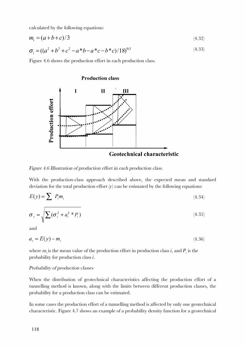
118

calculated by the following equations:

(4.32)

(4.33)

Figure 4.6 shows the production effort in each production class.

Figure 4.6 Illustration of production effort in each production class.

With the production-class approach described above, the expected mean and standard deviation for the total production effort (y) can be estimated by the following equations:

(4.34)

(4.35)

and

(4.36)

where mi is the mean value of the production effort in production class i, and P

i is the

probability for production class i.

Probability of production classes

When the distribution of geotechnical characteristics affecting the production effort of a tunnelling method is known, along with the limits between different production classes, the probability for a production class can be estimated.

In some cases the production effort of a tunnelling method is affected by only one geotechnical characteristic. Figure 4.7 shows an example of a probability density function for a geotechnical

119

characteristic affecting the production effort, and the limits between the different production classes. The probability for each production class can be estimated from the distributions of the geotechnical characteristic. The figure also shows the distribution of the production effort in each production class. In the actual case the distribution is triangular.

Figure 4.7 Example of the probability density function of a geotechnical characteristic affecting

the production effort, and the limits between different production classes.

Often however, two or more geotechnical characteristics affect the production effort. The production effort can be described with respect to these components as a curve in a space. Determination of the production effort can in this case be complicated. One way to estimate the probability for production classes is to take random samples from the distribution of each of the geotechnical characteristics and compare them with the method-specific limit for the characteristics. The characteristics are often assumed to be uncorrelated. A correlation between the characteristics can, however, also be regarded. Figure 4.8 shows an example of the limits between Production classes I-III, for two geotechnical characteristics x

1 and x

2 affecting

the production effort.

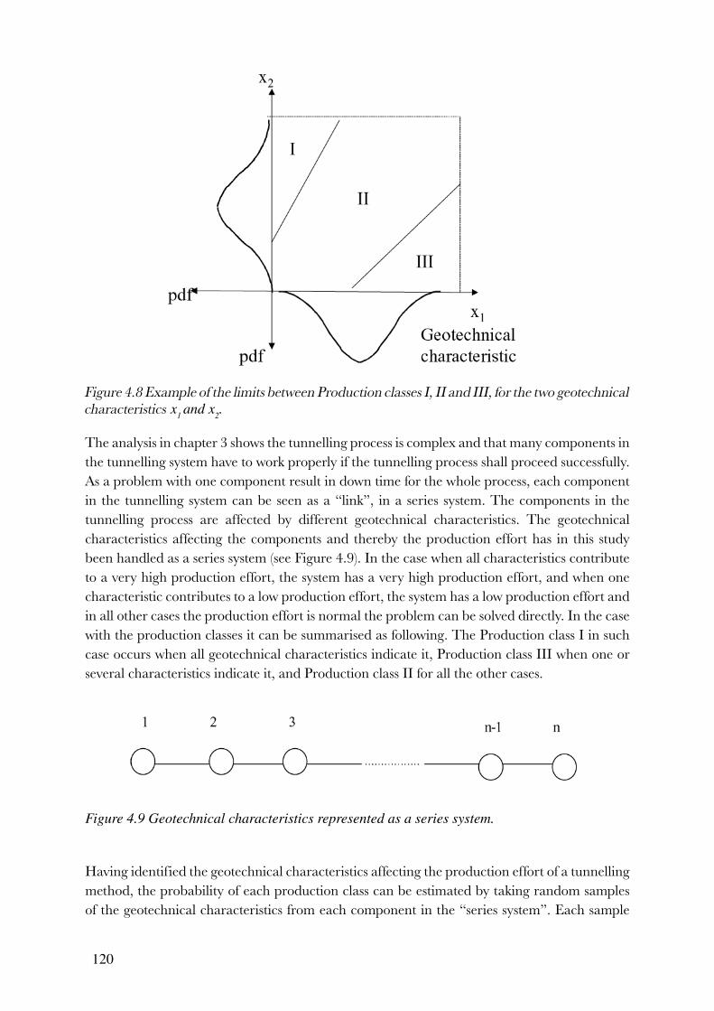
120

Figure 4.8 Example of the limits between Production classes I, II and III, for the two geotechnical

characteristics x1 and x

2.

The analysis in chapter 3 shows the tunnelling process is complex and that many components in the tunnelling system have to work properly if the tunnelling process shall proceed successfully. As a problem with one component result in down time for the whole process, each component in the tunnelling system can be seen as a “link”, in a series system. The components in the tunnelling process are affected by different geotechnical characteristics. The geotechnical characteristics affecting the components and thereby the production effort has in this study been handled as a series system (see Figure 4.9). In the case when all characteristics contribute to a very high production effort, the system has a very high production effort, and when one characteristic contributes to a low production effort, the system has a low production effort and in all other cases the production effort is normal the problem can be solved directly. In the case with the production classes it can be summarised as following. The Production class I in such case occurs when all geotechnical characteristics indicate it, Production class III when one or several characteristics indicate it, and Production class II for all the other cases.

Figure 4.9 Geotechnical characteristics represented as a series system.

Having identified the geotechnical characteristics affecting the production effort of a tunnelling method, the probability of each production class can be estimated by taking random samples of the geotechnical characteristics from each component in the “series system”. Each sample

121

can be seen as a Boolean variable having the value 0 or 1. With three production classes, two different estimations must be made. Where the sample is, “Production classes I or II” (value of 1) or “Production class III” (value of 0), “Production class I” (1) or “Production classes II or III” (0), then the Boolean variables S

z and M

z are defined as:

(4.37)

and

(4.38)

The series system values Ss and M

s in the respective cases can be estimated as the product of all

the components included in the series system as follows:

(4.39)

and

(4.40)

where Sz and M

z are components in the system.

The probability of the different production classes for the total system (ST) can be estimated by

the following equations:

(4.41)

(4.42)

(4.43)

Robustness

As discussed in Chapters 2 and 3, robustness-increasing measures can be applied to tunnelling methods in order to extend their range of geological application and to reduce the probability and consequences of undesirable events. The production effort required can also be reduced when robustness-increasing measures are used. Robustness-increasing measures can include for example improving the organisation or tunnelling equipment. Figure 4.10 shows the increased range of Production class I and II when robustness-increasing measures are used.

122

Figure 4.10 The influence of robustness-increasing measures on the probabilities of production

classes.

4.3.4 Modelling undesirable events

The “exceptional” time and cost can be estimated from knowledge about the probability and consequences of undesirable events. Different undesirable events have different probabilities and consequences. Some undesirable events depend on the productivity of the method, others do not. Undesirable events may have a low probability and major consequences, for instance when the actual geotechnical characteristics differ significantly from those in the normal application range of the method, and the method may have to be changed. Other undesirable events have a high probability and minor consequences, for example a minor breakdown.

A division into different event types has been made in order to, (a) obtain a distinct division between causes, probabilities and consequences, and (b) to enable a relation between undesirable events and production effort.

It must be emphasized that the risk analysis must include not only event types that are well known, but facilitate full and detailed analysis. In practice, there seems to be a tendency to overestimate the importance of those risks that can be evaluated with established methods.

As described in Chapter 3, there are different types of undesirable events. One suggestion for the classification of types of undesirable events is seen in Table 4.2. Undesirable events not covered by the first four types of undesirable events defined in Table 4.2 fall into the category “Miscellaneous”. Clearly other classification systems are possible, but this one has been used in the estimation model.

123

Table 4.2 Classification of types of undesirable events.

Type of undesirable event Definition Example

Production-dependent geological events.

Exceeding the limit of geotechnical characteristics where the method works fair, i.e. production class II.

Joint fractioning, compressive strength, water pressure/permeability.

Randomly-occurring geological events.

Locally-significant deviations of geological conditions.

Water-bearing zones,fault zones.

Randomly-occurring mechanical events.

Component failure in the machinery or equipment used.

Main bearing failure.

Randomly-occurring gross errors.

Consequences of lack of competence.

Incorrect design, insufficient organisation, quality control or experience; insufficient knowledge about the method’s working range.

Miscellaneous

Estimations of the probability and consequences of each undesirable event type can be made using risk analysis (Rausand, 1991), and involves:

− a description of the system, − risk identification, − estimation of the probability, − estimation of the consequences, and − risk reduction.

Risk identification consists of studying various tunnel projects, the undesirable events of which are analysed. In risk identification, experiences from similar combinations of geological conditions and tunnelling methods should be studied, but as the number of projects is limited, other combinations must also be considered. Risk identification in tunnelling projects has been discussed in Chapter 2. The statistical material obtained from risk identification can be used as a basis for the estimation of probabilities and consequences.

There are different ways to estimate the probability of undesirable events, for example utilising statistic data, or quantitative subjective estimates.

There are some difficulties however with estimating the probability from statistic data (Andersson, 1997), including for example:

− the shortage of reliable data on undesirable events,− the diversity and increasing improvements being made in tunnelling machines and

equipment design, size, purpose, and manufacture, − the diversity of geological conditions, and − the influence of project management.

124

When data on undesirable events using different combinations of tunnelling methods and geological conditions are limited, subjective estimates of probability often have to be made.

Production-dependent geological events—that is the probability to exceed the limit where the method works fair, i.e. production class II—is estimated using probability theory (elementary statistics) (Benjamin & Cornell, 1970). Where the probability density function of the geotechnical characteristic X is f(x), then the probability that the factor exceeds the critical value x

c is given

by:

(4.44)

This probability is guilty for each round in the studied zone. Figure 4.11 illustrates the probability of reaching the limit x

c .

Figure 4.11 Probability of exceeding the limit xc .

The probability P for x rounds that fails is calculated using Binominal distribution according to:

(4.45)

where n is the total number of rounds in the studied zone.

A binominal distribution with probabilities for each x number of failures is obtained. From this distribution is then the number x failures randomly taken in a Monte Carlo simulation, and then multiplied with the consequence for that number of failures.

If the total number of rounds n is increasing and the probability p is decreasing, the probability for failure can be made using Poisson distribution (Benjamin & Cornell, 1970). Poisson distribution is further discussed for calculation of random-occurring geological events. As discussed in Chapter 3, the consequences of production-dependent geological events often involves a standstill in order to make necessary improvements to the ground, or in the worst case even changing the tunnelling method, which results in downtime to establish new equipment. If the method has to be changed, this may result in a slower advance rate due to an initial learning

125

period. The consequence can involve weeks or months of extra time.

Clearly, the time and cost for production dependent geological events can be included in the normal as well as the exceptional time and cost. It has, however been decided that they shall be included in the exceptional time and cost. One reason for this is that the parties depending on their contractual situation can handle them differently.

Randomly-occurring geologically events can be handled as discrete random variables (Sturk, 1998). Poisson distribution, often applied in modelling the number of occurrences of events within a specified time or space interval, can be used in this case (Priest, 1993; Priest & Hudson, 1976; Baecher et al.,1977; Snow, 1970). Figure 4.12 illustrates Poisson distribution (after Benjamin & Cornell, 1970).

Figure 4.12 Probability mass function of a Poisson-distributed, discrete random variable, after

Benjamin and Cornell (1970).

The random variable X is the number of randomly-occurring geological undesirable events in the tunnel length L. The probability that x undesirable events occurs in the length L then becomes:

(4.46)

where x is the number of randomly-occurring geological undesirable events over the length L, λ is the number of randomly-occurring geological undesirable events per unit length, and L is the length of tunnel. The mean value of the number of events can be estimated as: λ L.

As discussed in Chapter 3, the consequences of randomly-occurring geological events often involve major standstills in order to restore the geological conditions to the state prior to the event and to continue with the excavation. This may include ground improvements or pumping water inflows out of the tunnel.

Randomly-occurring mechanical events, such as the failure of a machine component, can be handled as random variables. By observing the components over time, the problem can be

126

reduced to a one-dimensional problem involving time as the only random variable. The events are in this case discrete, and the time to failure continuous. The following methods used to estimate the probability and consequences of this undesirable event type are based on the work of Harr (1987), Henley and Kumamoto (1981), and Kapur and Lamberson (1987).

The probability of failure in a component of the system within a time interval (0,t) can be expressed as:

(4.47)

where f(τ) is the failure density function.

Failure rate is the probability that a failure occurs in a particular time interval—failure per unit time—given that a failure has not occurred prior to time t. The hazard function h(t) is the limit of the failure rate as ∆t approaches zero. Thus, the hazard function is the instantaneous failure rate and indicates the change in the failure rate over the operating time of the system or its components. The failure density function can be expressed as:

(4.48)

Typical for processes depending on the reliability of machine components, is that the initial failure rate is higher than that encountered later on because of various manufacturing and assembling defects. After this initial period, during which defective parts are replaced, the reliability improves again and the failure rate becomes almost constant for some time before increasing as the components wear out. The hazard function of this type of failure follows the so-called “bathtub curve” (see Figure 4.13). The curve can be approximated as a piecewise-linear function.

Figure 4.13 Example of a hazard function typical for machine components, the bathtub curve.

When the failure rate of one component is constant, for example where (h(t) = λ) is constant, the failure density function with time is:

(4.49)

where λ is the number of failures per unit time.

The probability of failure of the system during the construction time (t) can then be calculated according to Equations 4.50 to 4.51, as:

127

(4.50)

The tunnelling process can be seen as a “series” system consisting of several components, each of which must function if the whole process is to function. The probability of failure (P

s) of the

system is given by:

(4.51)

where Pi is equal to ( ) and is the probability of failure of the ith

component.

Where it can be assumed that the failure density function of all i components follows the exponential distribution, the probability of failure of the ith component is (1 – exp-(λ

it)). The

probability of failure of the whole system over the time period (0,t) then becomes:

(4.52)

The consequences of randomly-occurring mechanical undesirable events can be estimated by considering the “failed state” condition of the components, as they lead to downtime in the tunnelling process. The downtime depends on factors such as, (a) the components’ mean time to failure (MTTF), that is the expected time elapsing prior to failure, and (b) the mean time to repair (MTTR). The mean time to failure of one component can be expressed by:

(4.53)

The MTTF for a system consisting of several components can be estimated by:

(4.54)

Normally the components of a system that fails are repairable. Similar to the failure density function, the repair density function g(t) describes the random characteristics of the time required to repair a failed component when failure occurs at time zero. The repair rate r(t) corresponds to the hazard function and is the probability that the component is repaired in a unit time, given that the component failed at time zero, and is still not repaired at time t. The repair density function is related to the repair rate (r(t)) by:

(4.55)

The mean time to repair (MTTR) is the expected value of the time taken for repairing a failed component, expressed as:

(4.56)

When the repair rate is η and the repair density function is given by:

(4.57)

then the MTTR becomes:

(4.58)

128

From the above, it follows that a component is either in an operative state, or a failed state awaiting or being repaired. The probability that a component is in operating condition at time t, given that the component was as good as new at time zero is called A(t). The probability that a component is in a failed state at time t is called U(t). Thus operating and failed state conditions are complementary events, therefore:

(4.59)

Using exponential failure and repair density functions where the failure rates and repair rates are constants equal to their respective parameters, the following equations for the operative and failed state conditions can be derived by:

(4.60)

and

(4.61)

As the time (t) increases, U and A tend towards constant values. After a long period, t approaches infinity, the stationary failure state U (∞), and the stationary operative state A (∞), which are given by:

(4.62)

(4.63)

The consequences in terms of downtime when the system is in the failure state can be estimated from the above.

Randomly-occurring gross errors are difficult to handle in quantitative risk analysis. It is not possible to use the same analysis methods with respect to human factors as it is on technical components. There has therefore been a demand for the methods to facilitate the quantification of human reliability. Different methods used for estimating probability and the consequences due to human errors have been discussed in the literature by Rausand (1991), and for example include:

− the Technique for Human Error Rate Prediction (THERP), − the Success Likelihood Index Method (SLIM), − the Prediction of Operator Failure rate (PROF), and − Action Error Analysis (AEA).

The THERP method has been developed to predict human reliability and evaluate the impact of human failures on complicated human-machine-systems. This method is mainly based on the principle of event tree analysis (see Figure 4.14). In the analysis, the human operations that may contribute to failure of the actual system are identified, the probability and consequences of human error for each relevant human operation is estimated, and risk-reducing measures are suggested.

129

Figure 4.14. Example of an event tree—operator reaction on alarm, after Rausand (1991).

The THERP method has been used in the nuclear power and processing industry. The SLIM and PROF are methods have been used to handle insufficient-experience data about human reliability. SLIM is a technique used to estimate the probability of human errors in knowledge-based tasks. In this method, different factors affecting the probability of failure (Performance Shaping Factors—PSFs) are evaluated by expert estimates. Experts evaluate factors, such as the relative weight and value from each PSF for the actual task. The PROF is also a quantitative model for the estimation of probability of human errors based on expert evaluations. Factors like the quality of the information, back information, time pressure, risk exposure, and personnel skill and experience are included in the model.

In AEA, checklists for possible causes and consequences of human errors are made. Probability can be estimated by using a database of failure rates and PSFs.

Experience with the abovementioned methods in the estimation of the probability and consequences of human errors are limited, and therefore the results of these methods are only able to be provided in an approximate order of magnitude rather than more accurately. They do however provide a way to handle the impact of human factors on the tunnelling process.

Undesirable events that cannot be included in any of the groups described above may also occur. In the model, these events are called miscellaneous events.

4.4 Conclusions

The importance to the client and contractor of having at their disposal a good basis for making decisions about the budget and tender pricing was concluded from Chapter 2. Both parties need to obtain the distribution of total time and cost as a basis for making decisions. Furthermore, the construction-contracting method and the stage of the project both affect which party (client or contractor) is responsible for the increases in time and cost that may occur in response to different risk factors. Therefore these should be able to be considered as part of the basis for making decisions.

130

The theoretical estimation model can be summarised into the following steps based on discussions about the estimation model and practical modelling.

1. Determination of the geological and hydrogeological conditions along the

alignment of the tunnel.

2. Division of the tunnel into geotechnical zones with “homogeneous” geological

conditions, and selection of a tunnelling method suited to the actual

conditions.

A geotechnical zone is defined as a “a reach of tunnel modelled as having similar geotechnical conditions, in which the one tunnelling method is intended to be used”.

3. Estimation of normal time and cost for each zone

Normal time and cost is the time or cost of constructing the tunnel project under normal circumstances. Normal time and cost is estimated in a similar way, independent of the partner in the process (contractor or client), and the type of contractual and other conditions for the given project. In this estimation model, normal time is estimated based on the production effort of the method, and the normal cost is divided into three cost types: time-dependent, quantity-dependent and fixed. For each cost type, the production effort (g(x(l))) as well as the cost variable (z) are estimated. The normal cost for a geotechnical zone with a tunnel length of L, is expressed as a function of the production effort and cost variable (z). The relationship between the geotechnical characteristics and the production effort is established first, and then the product of the effort and cost variables is integrated along the given tunnel length (L), (see Equation 4.9) below:

(4.9)

where i is the zone, g(x(l)) is the production effort and z is the cost variable.

3.I Estimation of for the production effort related to the time component (Qt) (the

normal time)

The production effort (g(x(l))) for time-dependent cost is the time (Qt), which

expresses the time taken for tunnelling per metre of tunnel along the critical path with the chosen method. This time is estimated according to the following steps.

3.Ia Determination of the distribution of the geotechnical characteristics that impact

on the production effort of the tunnelling method used.

3.Ib Determination of the production classes in each zone and for each geotechnical

characteristic—for example high, normal and low production efforts.

131

3.Ic Estimation of the probability of each production class

There are three ways to estimate the probability of a production class. When only one geotechnical characteristic affects the production effort, the probability can be estimated directly from the distribution of the characteristic. If there are two factors, Monte Carlo simulation is used to estimate the probability. In some cases, several geological characteristics affect the production effort as a “series” type system. Each of the random samples of the geotechnical characteristics in the series system is treated as a Boolean variable.

3.Id Estimation of the production effort

This is expressed as a stochastic variable, where the variables have been triangularly-distributed and are based on expert assessments. The mean value and standard deviation of the production effort in each production class is estimated using the following equations:

(4.32)

(4.33)

where a is the optimistic or lowest expected production effort, b is the probable production effort, and c is the pessimistic or highest expected production effort.

The expected mean value and standard deviation of the production effort in each zone is estimated using the following:

(4.34)

(4.35)

(4.36)

where mi is the mean value of the production effort in Production class i, P

i is

the

probability of achieving Production class i, and σi is the standard deviation of

the production effort in Production class i.

If the geotechnical characteristics are fully correlated (auto correlation), the standard deviation of the production effort is estimated using:

(4.8)

where L is the length of the tunnel reach.

The standard deviation for partial correlation (auto correlation) between the characteristics is estimated using:

132

(4.15)

where δl is the distance within which the geotechnical characteristic shows relatively strong auto correlation from one point to another.

3.II Estimation of the normal cost

The cost variable (z) has been regarded in the estimation model as an independent constant or stochastic variable. The normal cost in a zone can then be expressed as:

(4.27)

where j is the cost type.

Estimation of each of the cost types proceeds as follows.

3.IIa Estimation of time-dependent costs

As the cost variable and production effort are assumed to be independent, the following simplification is used.

(4.28)

where zt is the time dependent cost variable and Q

t is the normal time.

In this case, the cost variable is assumed to be a stochastic variable with triangular distribution. The expected value and variance of the resulting total time-dependent cost is calculated using Monte Carlo simulation.

3.IIb Estimation of the quantity-dependent costs

In this case, the production effort g(x(l)) is the quantity per metre of tunnel, and the cost variable corresponds to the material cost per unit length. As the cost variable and quantity are assumed to be independent, the following expression is used.

(4.29)

As this expression is too complex to solve, the following simplification is used instead:

(4.30)

In this case, the product of the cost variable and the quantities is assumed to be independent of rock class or geotechnical characteristic. The product is assumed to have triangular distribution and the length to be a constant, where the mean value and variance of the unit costs are estimated according to Equations 4.17 and 4.18.

133

3.IIc Estimation of fixed costs

The production effort g(x(l)) for fixed costs is independent of the tunnel length, and the cost variable corresponds to the fixed cost for the construction. As the cost variable is regarded as an independent stochastic variable and the effort as a constant equal to 1, the following simplification is used:

(4.31)

3.III Estimation of the total normal cost in a zone

This is done using the following equation:

(4.22)

where i is the zone and j is the type of time or cost variable.

4. Estimation of exceptional time and cost for each zone

As discussed in Chapters 2 and 3, undesirable events of different types can and do occur, causing exceptional time and cost. Which particular exceptional time and cost that ought to be considered in the estimation depends on the client or contractor’s respective responsibility (contractual and other conditions).

4.I Identification of undesirable events

Five types of undesirable events are identified: production-dependent geological events, randomly-occurring geological events, randomly-occurring mechanical events, gross errors, and miscellaneous.

4.II Estimation of the probability of the identified undesirable events.

4.IIa Estimation of the probability of production-dependent geological events

This is the probability of exceeding the limit in which the method works efficiently, and is calculated using probability theory. If the probability-density function of the geotechnical characteristic (X) is f(x), then the probability that the factor exceeds the critical value (x

c) is given by:

(4.44)

The probability (P) of x failures can be calculated using binominal distribution according to the following expression:

(4.45)

where n is the total number of rounds in the studied zone.

A binominal distribution with probabilities for each x number of failures is

134

obtained. From this distribution is then the number x failures randomly taken in a Monte Carlo simulation, and then multiplied with the consequence for that number of failures.

4.IIb Estimation of the probability of randomly-occurring geological events

Modelling the occurrence of a number of events within a specified interval of time or space is done using Poisson distribution. The random variable (X) is the number of randomly-occurring, geological, undesirable events along a tunnel of length L. The probability that just undesirable event x occurs in the length of tunnel L, is therefore given by:

(4.46)

where x is the number of events occurring over length l, λ is the number of events per unit length, and L is the tunnel length.

4.IIc Estimation of the probability of randomly-occurring mechanical events

This is done in relation to the failure rate of the machine components. The probability of failure of the whole system over the time period (0,t) is estimated as follows:

(4.52)

where λ is the number of failures per unit time (t).

4.IId Estimation of the probability of randomly-occurring gross errors

This is achieved using methods that quantify human reliability. One method developed to predict human reliability and evaluate the impact of human failures in complicated human-machine-systems is the THERP.

4.III Estimation of the consequences for each type of undesirable event identified

The consequences of these are often estimated as the cost of standstills and the cost of materials required, including for example rock support or spare parts.

4.IIIa The consequences of production-dependent geological events

This includes standstills resulting from ground improvement measures, or in the worst case scenario, changing the tunnelling method itself.

4.IIIb The consequences of randomly-occurring geological events

This includes major standstills caused by taking measures to reinforce ground conditions to the state they were in prior to the event.

135

4.IIIc The consequence of randomly-occurring mechanical events

This includes downtime in the tunnelling process caused by component failure. Downtime depends on factors such as the mean time to failure (MTTF) of the components—that is the expected working time before failure—and the mean time taken to repair the component (MTTR).

4.IV Estimation of the exceptional cost or time for each event type

The probability that an undesirable event occurs is described with Boolean variables. In this application, the random variable can exist in one of two conditions: (1) where the “undesirable event k occurs”, or (2) where the “undesirable event k does not occur”. The undesirable event occurs with probability (p), and “does not occur” with probability (1-p), according to the following:

(4.19)

The exceptional cost for each event type is estimated using the following:

(4.20)

The total exceptional cost is estimated as the sum of the exceptional time or cost for the different event types according to the following:

(4.21)

5. Calculation of the total time or cost using Monte Carlo simulation.

The total cost or time is expressed as the sum of normal time and cost, and exceptional time and cost for a given tunnelling method over all the geotechnical zones according to:

(4.22)

The parameters included in the model—such as advance rate—are expressed as stochastic variables. The outcomes from the estimation, are total construction costs (and completion time) presented as a distribution curve.

Calculation of the expected value of the total time or cost can be made using:

(4.23)

In the following two chapters, the estimation model is applied to case studies. The results obtained using the model are discussed and compared with the actual outcomes.

137

5 Case study – the Grauholz tunnel

5.1 Introduction

5.1.1 About the chapter

In this Chapter, the model for estimating the time and cost of tunnel projects (described in Chapter 4) is applied to the Grauholz Tunnel in Bern, Switzerland.

The aim of this chapter is to show that the results obtained from the estimation model are realistic. The total construction time and cost results obtained from the estimations are compared with the actual construction time and costs from this case study. A further aim is to show that following the estimation steps described in Chapter 4 makes the proposed estimation model clearer. As discussed in Chapter 2, different factors—such as the degree of correlation, the contractual situation and organisation, the machine type and its robustness—all affect decision-making as well as the results. The impact of these factors is also discussed in this chapter.

The Grauholz Tunnel has been chosen as a case study in this thesis in order to demonstrate the application of the estimation model to a well-defined project where different types of tunnelling machines can be considered.

5.1.2 Description of the project

The Grauholz Tunnel was built between 1990 and 1993. It is 5500 m long, and passes through moraine and sandstone. The tunnel forms part of the Mattstetten-Rothrist Link, and is situated near Bern in Switzerland (see Figure 5.1). The tunnel was built to enable traffic to by-pass the junction at Zollikofen, and has the capacity to be incorporated into the Swiss Railway Authority’s (Schweizerische Bundesbahn) planned expansion referred to as Bahn 2000.

Figure 5.1 Location of the Grauholz Tunnel, after Jancsez & Steiner (1994).

138

The geological conditions in the area are very complicated. The Schweizerische Bundesbahn (SBB) tried to minimise the length of the tunnel that had to run through moraine and water; therefore the major part of the tunnel was routed through sandstone (see Figure 5.2).

Figure 5.2 Overview of the Grauholz Tunnel route, after Scheidegger (1990).

The SBB envisaged that the tunnel would be excavated from both ends using open shields, combined in part with reinforcement or dewatering measures. In areas containing groundwater, a pilot tunnel and wells were planned to act as dewatering measures. Temporary reinforcement using jet grouting in front of the face was planned in areas characterised as being somewhere between soft ground and sandstone.

The lowest tender for the whole project exceeded SBB’s cost estimations by about 40%. One of the reasons for the cost excesses in the tenders was that tunnelling was planned from both directions. When tunnelling was planned from one direction only, the cost excess was reduced to just 12% over SBB’s original estimate. Since the contractors did not find SBB’s proposed tunnelling method optimal for the given conditions, alternative methods were proposed. As not all the quality requirements for these alternatives could be solved before the contract was signed, they were solved subsequently during construction. The manufacturer of the shield machine to be used to dig the tunnel was Herrenknecht, and the main contractors for the project forming a joint venture were Marti AG, Kopp AG, and Wayss & Freytag AG.

5.1.3 Geology and hydrogeology

Step 1

According to the model described, Step 1 includes a determination of the geological and hydrogeological conditions along the alignment of the tunnel. The soil in the area of the Grauholz Tunnel consisted of material of glacial epoch origin containing deposits of glaciofluvial sand and gravel covered by some metres of moraine (see Figure 5.3). The sandstone was a special type, which in alpine countries is referred to as molasse. Southeast of the tunnel axis lies a steep northwest flank of Upper Tertiary molasse.

Pre-investigations showed that streams and lakes had once existed in the vicinity, into which

139

glacial mud streams, silty and sandy sediments, and clayey, silty sediments had been deposited. This variety of materials confirmed that the sediments had moved rapidly from one place to another. Extensive pre-investigations were necessary to obtain the knowledge required about the geological conditions. In total, 45 core drillings, six water-jet drillings, six big-bore wells, 1.4 km of reflection seismic and 0.5 km of electromagnetic investigations were carried out in the area.

Figure 5.3 Geological section through the length of the Grauholz Tunnel, after Harsch (1990).

Table 5.1 shows the most important values for the geotechnical characteristics in the various geological layers surrounding the Grauholz Tunnel shown in Figure 5.3.

Table 5.1 Values for geotechnical characteristics of the geological layers found in the Grauholz

Tunnel; the mean values are from laboratory tests, the k values from pump tests, and the

values in parenthesis are subjective estimations, after Harsch (1990, 1994).

Layer USCS classification

Geology Density[kN/m3]

Friction angle [º]

Cohesion[kN/m2]

Conductivity[10-4 m/s]

Plasticity[%]

1 ML, SM Delta sediment 21.1 35.2 1.3 0.5 5.4

2 CL Sediment 21.4 19.0 420 <0.01 10.2

3 GC-CL Base moraine 22.0 Su = 445 <0.01 9.3

4 GM Moraine 22.8 42.8 (5) 0.2 4.8

5 GP, GW Glaciofluvial gravel, sand

(21.5) 43.3 - 32 -

6 Molasse 22.7-25.1 <0.05 -

* the compressive strength for the Molass have been estimated to 1-22 MPa G = gravel, S = sand, M = silt, C = clay,

W = well-graded material, P = uniformly-graded material, and L = low liquid limit

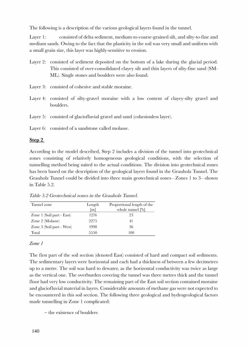
140

The following is a description of the various geological layers found in the tunnel.

Layer 1: consisted of delta sediment, medium-to-coarse-grained silt, and silty-to-fine and medium sands. Owing to the fact that the plasticity in the soil was very small and uniform with a small grain size, this layer was highly-sensitive to erosion.

Layer 2: consisted of sediment deposited on the bottom of a lake during the glacial period. This consisted of over-consolidated clayey silt and thin layers of silty-fine sand (SM-ML). Single stones and boulders were also found.

Layer 3: consisted of cohesive and stable moraine.

Layer 4: consisted of silty-gravel moraine with a low content of clayey-silty gravel and boulders.

Layer 5: consisted of glaciofluvial gravel and sand (cohesionless layer).

Layer 6: consisted of a sandstone called molasse.

Step 2

According to the model described, Step 2 includes a division of the tunnel into geotechnical zones consisting of relatively homogeneous geological conditions, with the selection of tunnelling method being suited to the actual conditions. The division into geotechnical zones has been based on the description of the geological layers found in the Grauholz Tunnel. The Grauholz Tunnel could be divided into three main geotechnical zones—Zones 1 to 3—shown in Table 5.2.

Table 5.2 Geotechnical zones in the Grauholz Tunnel.

Tunnel zone Length [m]

Proportional length of the whole tunnel [%]

Zone 1 (Soil part - East) 1276 23

Zone 2 (Molasse) 2275 41

Zone 3 (Soil part - West) 1998 36

Total 5550 100

Zone 1

The first part of the soil section (denoted East) consisted of hard and compact soil sediments. The sedimentary layers were horizontal and each had a thickness of between a few decimetres up to a metre. The soil was hard to dewater, as the horizontal conductivity was twice as large as the vertical one. The overburden covering the tunnel was three metres thick and the tunnel floor had very low conductivity. The remaining part of the East soil section contained moraine and glaciofluvial material in layers. Considerable amounts of methane gas were not expected to be encountered in this soil section. The following three geological and hydrogeological factors made tunnelling in Zone 1 complicated:

− the existence of boulders

141

− a lack of fines, and − high groundwater pressure coupled with limited dewatering possibilities.

Early on in the planning phase, it was stated that the excavation of Zone 1 could be complicated.

Zone 2

The sandstone part of the tunnel consisted of soft marl and sandstone (molasse). A special type of sandstone was found containing homogeneous sand without clay or silt. Normally the sandstone contained silty, fine sand. Owing to the thickness of the overburden (nearly 120 m), pre-investigations were not completed to the extent necessary for making reliable forecasts of the coarse-grain-sized medium sandstone. The sandstone was estimated to have a low to very low compressive strength. Owing to a groundwater pressure of 0.31 MPa on the tunnel floor, flowing ground could occur in this zone. Inflows of water and mud from the heading could also occur if the layer was not dewatered or stabilised in advance.

Zone 3

The soil part denoted West consisted of hard layers of silty-gravel moraine, containing clay and sand. Stones and boulders were also found in the whole soil section, and were situated above the groundwater level. Tests demonstrated that layers containing methane gas existed in this soil section. The test results of 1.6 volume-percent of methane in the soil section would however probably result in a concentration of <0.1 vol.-% when the tunnel was ventilated as per the requirements. Figure 5.4 shows the grain size distribution (without considering the boulders in the ground).

Figure 5.4 Grain size distribution of the soft soil section “West”, after Harsch (1990).

As shown in the Figure 5.4, the soil has a wide grain-size-distribution and varying overburden. This placed contradicting demands on the tunnelling method. The following section describes possible tunnelling methods for these geological conditions.

142

5.1.1 Tunnelling methods and corresponding robustness-increasing measures

Step 2 in the estimation model also includes making a choice of tunnelling method that could be suitable for the actual site conditions—geological, hydrogeological and organisational. The following three machine types were considered (Ruhrer, 1994):

− combined shield: able to be rebuilt from slurry to dry excavation;− EPB shield: where the soil mixture in the front supports the soil and water pressure

from the ground, and a screw conveyor transports the excavated material; and− open shield: without the ability to support the ground and water pressure at the

face; this shield cannot be used below the groundwater table if the soil has a high conductivity.

Different robustness-increasing measures can be applied to each type of shield machine. Therefore which robustness-increasing measures in particular to apply depends on the actual type of shield machine being used. When tunnelling with the combined shield, a high content of fines can cause problems with the separation. Separation can be performed using centrifuges or a band filter. There is a major difference between the material from the centrifuge where the bentonite is separated from fine-grain soil, and the material from the band filter where bentonite is removed together with the remaining material. Laboratory tests have shown that the height of the muck pile generated from a centrifugation set-up is reduced to one tenth, and to one third with the “band filter”. The time required for the reduction is also shorter for centrifuged material compared with using the band filter (Steiner, 1994). To avoid clogging the bore head, a separate centre cutter can be installed, or jet pipes on the dive wall.

When tunnelling with an EPB shield, the soil mixture in the working chamber supports the face. Unlike with the combined shield machine, it is not possible to integrate a stone crusher into the bore head. To obtain better consistency in the soil foam, various additives such as bentonite or polymers can be used.

Major problems can arise when tunnelling with an open shield machine in cohesionless soil below the water table. To increase the method’s robustness in this type of soil, measures such as lowering the groundwater with wells, vacuum lances or freezing can be used.

Shield machines and robustness-increasing measures used are described more in detail in Chapter 3. Estimation of total time and costs for the application of the different shield machines with a low and high degree of robustness is discussed in the following section.

5.2 Estimation of time and costs

5.2.1 Normal time and costs

According to the model described, Step 3 consists of the estimation of normal time and costs for constructing the tunnel. Normal cost is estimated according to Equation 4.9.

Step 3.I of the model consists of an estimation of the production effort for the time component Q

t for the zone.

143

Step 3.Ia of the model consists of a determination of the distribution of geotechnical characteristics that impact on the production effort of the particular tunnelling method being considered. In geotechnical Zones 1 and 3, the production effort for the shield machines—combined, EPB and open—are affected by the occurrence of boulders, fines and the combination of water pressure and conductivity. In geotechnical Zone 2, the production effort is affected by the compressive strength of the rock. Table 5.3 shows the values predicted for the geotechnical characteristics—the content of boulders, fines and the combination water pressure and conductivity—based on geological pre-investigations (Steiner, 1996). The distribution of the geotechnical characteristics is assumed to be rectangular. Rectangular distribution is used in this study as it could be assumed that there was major uncertainty in the results of the pre-investigations, due to they’re being random samples.

Table 5.3 Predicted values for geotechnical characteristics, after Steiner (1996).

Geotechnical characteristics

Unit Zone 1Min Max

Zone 2Min Max

Zone 3Min Max

Water pressure [MPa] 2.5 3.7 Not applicable Not applicable

Conductivity [m/s] 10-8 10-2 Not applicable Not applicable

Content of boulders

[%] 2 10 Not applicable 2 10

Content of fines

[%] 7 15 Not applicable 0.1 1.0

Compressive strength

[MPa] 1 22

Step 3.Ib consists of determination of production classes within each zone and for each geotechnical characteristics, for example high, normal and low production effort. In this case, three classes of production effort—high, normal and low—have been considered. The limits of geotechnical or groups of geotechnical characteristics, which correspond to a change between production classes have also to be defined. The values in this study are called method-specific limits. Table 5.4 shows the limits of the geotechnical characteristics—content of boulders, fines and the combination water pressure and conductivity—for the shield machines studied. The values for the limits are based on interviews with Steiner (1997), Aebersold (1997) and Thewes (1997), and are therefore subjective estimations.

144

Table 5.4 Estimation of the limits between the different production classes for various

geotechnical characteristics and shield machines with different degrees of robustness, where

A = water pressure [bar], G = conductivity [m/s], B = content of boulders [%], C = content of

fines [%], and D = compressive strength [MPa].

Geotechnical characteristic Production class

I II III

Combined shield with low robustnessA/G

BC

D

A<3 / G<10-3A<2/G<5*10-3

<36<C<9

20<D<40

3<A<6/G=10-3A=2/5*10-3<G<10-2

3<B<55<C<69<C<105<D<20

40<D<50

A>6/G>10-3A>2/G>10-2

>5<5

>10<5

>50EPB shield with low robustnessA/G

BCD

A<0.5 /G<10-5A<1/G<10-5

<240<C<70

20<D<40

1<A<3/G=10-50.5<A<1/5*10-5<G<10-3

2<B<330<C<40

5<D<2040<D<50

A>3/G>10-5A>1/G>10-3

>3>70<30 <5>50

Open shield with low robustnessA/G

BCD

A<1 /G<10-6A<0.5/G<5*10-6

0<B<1050<C<10020<D<40

A=1/G=10-6A=0.5/5*10-6<G<10-5

10<B<10020<C<505<D<20

40<D<50

A>1/G>10-6A>0.5/G>10-5

-<50<5

>50Combined shield with high robustnessA/G

BC

D

A<3 / G<10-3A<2/G<5*10-3

<55<C<11

20<D<40

5<A<6/5*10-4<G<10-3A=2/5*10-3<G<10-2

5<B<100<C<5

11<C<155<D<20

40<D<50

A>6/G>10-3A>2/G>10-2

>10>15 <5>50

EPB shield with high robustnessA/G

BC

D

A<2/G<10-5 A<0.5 /G<5*10-5

<230<C<7020<D<40

2<A<5/10-4<G<10-50.5<A<1.5/5E-5<G<10-3

2<B<30<C<305<D<20

40<D<50

A>5/G>10-4A>1.5/G>10-3

>10>70 <5>50

Open shield with high robustnessA/G

BC

D

A<2/G<10-4A<1/G<10-3

0<B<2030<C<10020<D<40

2<A<3/G=10-4A=0.5/5*10-3

20<B<1000<C<305<D<20

40<D<50

A>3/G>10-4A>0.5/G>10-3

--

<5>50

Figures 5.5 and 5.6 illustrate the limits between the various production classes defined for different geotechnical characteristics using combined, EPB and open shield machines respectively, with a low degree of robustness based on Table 5.4. The predicted range of the

145

geotechnical characteristics shown in these figures is based on Table 5.3. Figure 5.5 illustrates the relationship between production class and the content of fines, while Figure 5.6 shows the content of boulders. Figure 5.7 illustrates the limits between Production classes II and III for the combination of the geotechnical characteristics—conductivity and water pressure—for combined, EPB and open shield machines. Lower values than these limits for the geotechnical characteristics mean that the respective method falls into Production class II (or I), and higher values than these limits indicate Production class III.

Figure 5.5 Relationship between production class and the content of fines (low method-

robustness).

Figure 5.6 Relationship between production effort and the content of boulders (low method-

robustness).

146

Figure 5.7 Limits between Production classes II and III, with low method-robustness, for the

combination of conductivity and water pressure.

Step 3.Ic of the model consists of an estimation of the probability for each production class. In the case studied here, the geotechnical characteristics are assumed to affect the production effort as though it were a series system (see Figure 5.8).

Figure 5.8 Geotechnical characteristics presented as a series system affecting the production

effort when using combined shield, EPB shield and open shield machines.

The limits for each respective production class in Table 5.4 have been compared with the range of results found in the pre-investigations of the geotechnical characteristics in Table 5.3. Monte Carlo simulation has been used to estimate the probability for each production class according to equation 4.37-4.43. Table 5.5 shows the results of the simulation. This table shows that with a low degree of machine robustness in Zone 1, the combined shield has the highest probability of falling into Production classes I or II, as the combination of water pressure and conductivity, and the amount of boulders are always within admissible limits—only the limit of the content of fines is exceeded with a certain probability. The EPB and open shields with a low degree of robustness measured in Zone 1, always have some factor exceeding the limit for Production classes I or II.

147

Table 5.5 Probabilities for different production classes by zone, shield machine and degree of

robustness

Production

class

Combined shield EPB shield Open shield

Low degree of robustness

High degree of robustness





Zone 1

I 0.03 0.07 0 0 0 0

II 0.12 0.93 0 0.01 0 0.38

III 0.85 0 1 0.99 1 0.62

Zone 2

I 0.09 0.09 0.09 0.09 0.09 0.09

II 0.72 0.72 0.72 0.72 0.72 0.72

III 0.19 0.19 0.19 0.19 0.19 0.19

Zone 3

I 0 0 0 0 0 0

II 0 0 0 0.13 0 1

III 1 1 1 0.87 1 0

Step 3.Id in the model consists of an estimation of the production effort for the time component in each production class. The production effort in each production class is expressed as a stochastic variable with triangular distribution, involving the estimation of (a) an optimistic value with the lowest-expected production effort, (b) a neutral value for the probable production effort, and (c) a pessimistic value for the highest-expected production effort. As discussed, the tunnelling process can be described as a cyclical process, consisting of different unit operations. The production effort g(x(l)) can be expressed as the sum of the times for each of the unit operations (t

i) in hours per metre (h/m), (see Equation 5.1). The operations are assumed to be

uncorrelated.

(5.1)

where ti is the time measured in hours for the different unit operations required for digging one metre of tunnel. The unit tunnelling operations can for example be: excavation, installing concrete segments, changing cutter(s), and various other operations that can lead to down time. The time for excavation depends for example on the rotation speed of the cutter head and the penetration rate. Down time can depend on for example, the failure of a component, problems with the slurry system, waiting time for spare parts, geological surveying, or the maintenance of machinery (which can for example be about one month per year, including a complete examination of the machine).

Table 5.6 shows the constants used in the estimation of production effort. These values are based on experience from shield and TBM projects in Switzerland, for example the Kraftwerk Amsteg and Adler tunnels.

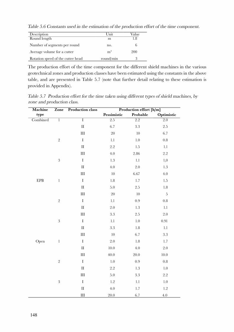
148

Table 5.6 Constants used in the estimation of the production effort of the time component.

Description Unit ValueRound length m 1.8

Number of segments per round no. 6

Average volume for a cutter m3 200

Rotation speed of the cutter head round/min 3

The production effort of the time component for the different shield machines in the various geotechnical zones and production classes have been estimated using the constants in the above table, and are presented in Table 5.7 (note that further detail relating to these estimation is provided in Appendix).

Table 5.7 Production effort for the time taken using different types of shield machines, by

zone and production class.

Machine

type

Zone Production class Production effort [h/m]

Pessimistic Probable Optimistic

Combined 1 I 2.5 2.2 2.0

II 6.7 3.3 2.5

III 20 10 6.7

2 I 1.1 1.0 0.8

II 2.2 1.5 1.1

III 4.0 2.86 2.2

3 I 1.3 1.1 1,0

II 4.0 2.0 1.3

III 10 6.67 4.0

EPB 1 I 1.8 1.7 1.5

II 5.0 2.5 1.8

III 20 10 5

2 I 1.1 0.9 0.8

II 2.0 1.3 1.1

III 3.3 2.5 2.0

3 I 1.1 1.0 0.91

II 3.3 1.8 1.1

III 10 6.7 3.3

Open 1 I 2.0 1.8 1.7

II 10.0 4.0 2.0

III 40.0 20.0 10.0

2 I 1.0 0.9 0.8

II 2.2 1.3 1.0

III 5.0 3.3 2.2

3 I 1.2 1.1 1.0

II 4.0 1.7 1.2

III 20.0 6.7 4.0

149

Looking at the probabilities for the production classes in Table 5.5, and the production efforts in Table 5.7, the mean and standard deviation of the production effort for the time component in each production class is estimated according to Equations 4.32 and 4.33. Based on these values, the resulting expected production effort for the time for each zone has been estimated according to Equation 4.34. Estimation of the variation for full correlation has been done according to Equations 4.8 and 4.35, where L is the zone length; and part correlation has been made according to Equation 4.15. Based on the geological investigations and the subjective estimations, it has been assumed that Zone 2 is more homogeneous, and Zones 1 and 3 are more heterogeneous (in Figure 5.13 it can also be seen that the actual production effort frequently changed in Zones 1 and 3, but was more constant in Zone 2). It has been assumed that the distance within which the geotechnical characteristics show relatively strong correlation from one point to another is 100 m in Zones 1 and 3, and 400 m in Zone 2. Table 5.8 shows the mean and standard deviation of the normal construction time for different types of shield machines and degrees of robustness.

Table 5.8 Normal construction time by machine type, degree of robustness and zone.

Machine type Combined shield EPB shield Open shield


ZoneExpected time [mth]

1 2 3

30 9 30Tot. 69

1 2 3

32.4 8 29 Tot. 69

1 2 3

64.7 9.1 44 Tot.117.8

Variation [mth] -- fully correlated 1.8 3.7 5.8 13.7 8.9 3.0 6.2 11.3 18 5 15 24- partially correlated 3.3 1.6 1.3 3.9 2.3 1.3 1.4 3.0 5 2 3 6.2


ZoneExpected time [mth]

1 2 3

11.2 9 30 Tot.50.2

1 2 3

32.4 8.1 26.4Tot.66.9

1 2 3

45.7 9.1 9.9Tot.64.7

Variation [mth] - - fully correlated 2.8 3.3 5.3 6.8 9.1 3.0 9.2 13.3 30 5 15 34- partially correlated 0.8 1.3 1.2 1.9 2.6 1.3 2.0 3.5 8 2 3 8.8

Step 3.II in the estimation model consists of an estimation of the normal cost according to Equation 4.27. The normal cost types considered in this study are: quantity dependent, time dependent and fixed. The costs are estimated according to common cost estimation methods where some values are expressed as stochastic variables with triangular distribution. The values used in the cost estimation are based on the author’s experience gathered during several years work with time and cost estimations of similar tunnel projects (see Isaksson, 1998).

In this study, the time and cost for different tunnelling methods (shield machines) estimated using the model, is compared with the actual results of the underground work. It was not considered necessary to undertake a complete estimation for this particular study—including for instance preliminary groundwork for the whole project. Table 5.9 presents those factors that were considered as well as those that were not considered in the estimation.

150

Table 5.9 Time and cost factors that were considered and “not considered” in the estimation.

Considered Not considered * Excavation and permanent support with low and

high degrees of robustness. * Site “mobilisation” and “demobilisation” and

staffing of the contractor’s site office during the whole construction period.

* Transporting, installing and dismantling of the shield machine.

* Cutting and covering tunnels, locations, entrances and installations in the tunnel.

* Transportation of muck from the tunnel entrances and beyond.

* Cost excesses due to increases in wages.* Groundwork.* Geological pre-investigations.

The cost for various robustness-increasing measures—for example for enhancing the machine or other necessary equipment, or for improving the ground conditions—have been estimated as a percentage of the shield-machine method price. In this case, it could increase the cost by about 20-40%. If expensive measures such as freezing or jet grouting are needed, they may increase the total cost by about 50%. The costs for bentonite are higher when using a band filter, and the problems associated with consolidation of the muck pile also increase the price. These costs must be compared with the higher costs for incorporating centrifugation into the method. The costs for different robustness-increasing measures are shown in Table 5.10.

Table 5.10 Estimated costs in Swedish kronor [SEK] for robustness-increasing measures for

shield machines.

Machine

Type

Reasons for application Robustness-increasing

measures

Costs

[SEK]

Combined High clay content

Cutter changes

CentrifugesSeparate centre cutterWear layers on cutters

2,000,0001,000,000

160,000EPB Low cohesion

Cutter changesAdditivesWear layers on cutters

2-- 160,000

Open High water pressure Dewatering measures 3200

1Per unit; 2additive specific; 3per metre.

Step 3.IIa of the estimation model consists of estimating the time-dependent costs. The time-dependent costs in this study include the costs for:

− site office and personnel, − machinery, and − labour.

The costs for a site office and site-office personnel includes wages and salaries for eight employees and associated office materials, and are denoted by z

t1. The cost for machinery and

equipment used during the main construction period per month are denoted by zt2, and the

cost for tunnelling machines used during the main construction period per month are denoted by z

t3. The cost of labour per month (denoted by z

t4) are estimated assuming a working period

of 23 days per month. Table 5.11 shows the time-dependent cost for the different machine types expressed in millions of Swedish kronor per month (MSEK/mth). The differences in the time-

151

dependent costs for a combined shield and an EPB shield are due to the separation equipment needed for combined shield machines but not for EPB shield machines.

Table 5.11 Estimated values of time-dependent costs in millions of Swedish kronor per month

[MSEK/mth], where zt1 = the cost for site office and personnel, zt2 = the cost for general

machines, zt3 = the cost for tunnelling machines, and zt4 = the cost for labour.

Type of machine Time-dependent costs [MSEK]

zt1

zt2

zt3

zt4

Low/high degree of robustness

Combined shieldMinimumLikeliestMaximum

1.11.21.5

0.170.200.24

0.630.630.63

2.53.63.9

EPB shieldMinimumLikeliestMaximum

1.11.21.5

0.170.200.24

0.260.270.27

2.53.63.9

Open shieldMinimumLikeliestMaximum

1.11.21.5

0.160.200.23

0.280.290.29

2.53.63.9

Step 3.IIb in the estimation model consists of the estimation of quantity-dependent costs. The

quantity-dependent costs are in this case, costs for the quantity of various materials required

per metre of constructed tunnel, such as the cost of construction materials, wear and tear,

fuel, electricity and permanent rock supporting with concrete segments. These segments

are understood to be about 40 cm thick, and the space between concrete segments and the

surrounding ground to be 10 cm. Table 5.12 shows the estimated probable consumption of

grout, bentonite and freshwater for a tunnel with a diameter of 12 m.

Table 5.12 Estimated probable consumption of construction material using a combined shield

machine.

Construction

material

Consumption of materials

per metre of finished tunnel

Grout [tonne/m] 9.1

Bentonite [tonne/m] 1.4

Water [m3/m] 123

For some quantity-dependent costs, the cost variable (zq) and for others, the production

effort (Qq), (expressed in metres of tunnel) is expressed as a stochastic variable with triangular

distribution. The product of the factors—cost variable and production effort—is then triangularly distributed. Table 5.13 shows the quantity-dependent cost for each type of shield machine. The reason behind the lower construction material costs (z

q) for EPB and open shield

machines, compared with combined shield machines, is they do not require separation and bentonite.

152

Table 5.13 Estimated values for quantity-dependent cost in millions of Swedish kronor per

metre of tunnel (MSEK/m), where zqQq = the cost of construction material.

Type of machine Quantity-dependent costs [MSEK/m]

zqQ

qlow robustness

zqQ

qhigh robustness


0.0620.0690.077

0.0620.0690.077


0.0630.0650.067

0.060.070.08


0.0580.0630.075

0.090.110.13

Step 3.IIc of the estimation model consists of an estimation of fixed costs. The production effort (Q

f ) is in this case, a constant equal to 1. In this study, the fixed cost is the cost for site

“mobilisation and demobilisation” (zf1), and the cost of the shield machine (z

f2). These costs can

be estimated using common estimation methods, and are assumed to be stochastic variables with triangular distribution. Table 5.14 shows the fixed cost for each type of shield machine. The lower cost of using open shield machines, compared with combined shield machines, depends on their lower degree of complexity.

Table 5.14 Estimated values of fixed costs in millions of Swedish kronor [MSEK], where zf1 =

the cost of site “mobilisation and demobilisation”, and zf2 = the cost of shield machines.

Type of machine Fixed costs [MSEK]

zf1

Low/high robustness

zf2

Low robustness

zf2

High robustness


30.131.733.3

105132150

110141162


26.928.329.3

93118134

93118134


31.131.733.3

617993

617993

Step 3.III of the model consists of an estimation of the normal cost as the sum of the product of the factors—production effort and cost variable—according to Equation 4.9. Table 5.15 shows the normal costs for the respective cost type. The result of the Monte Carlo simulation

153

of the normal cost is expressed by the following values: likeliest, minimum, maximum. In the triangular distribution of for example, the quantity-dependent and fixed costs, the minimum and maximum values of the results are correct. For time-dependent costs however, there are stochastic variables with distributions other than triangular. This means that the correct result should be expressed as a mean value with standard deviation. The tables and figures in this study, however, show the mean, minimum and maximum values obtained from the simulation considering partial correlation.

Table 5.15 Estimated values for the different types of normal costs in millions of Swedish

kronor [MSEK], where CNq = quantity-dependent costs, CNf = fixed costs, and CNt = time-

dependent costs.

Machine type Normal costs [MSEK]

CNq

low

robustness

CNf

low

robustness

C Nt

low

robustness

CNq

high

robustness

CNf

high

robustness

C Nt

high

robustness

Combined shieldMinimumMeanMaximum

344385429

136161183

276375481

344385429

140169195

200273347

EPB shieldMinimumMeanMaximum

350360370

120143163

262353437

356392420

120143163

245336434

Open shieldMinimumMeanMaximum

320360393

92109 126

440599778

500613717

92109126

135328554

Table 5.16 shows the expected normal cost and variation for full and partial correlations. The expected normal cost has been estimated according to Equation 4.9. Estimation of the variation for full correlation has been made according to Equations 4.8 and 4.35, where L is the zone length. Estimation of the partial correlation has been made according to Equation 4.15. Based on subjective estimation, it has been assumed that the distance within which the geotechnical characteristics show relatively strong correlation from one point to another is 100 m in Zones 1 and 3, and 400 m in Zone 2.

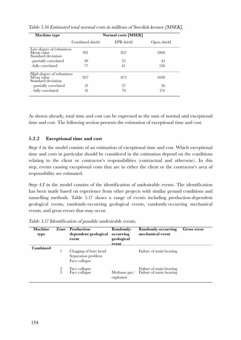
154

Table 5.16 Estimated total normal costs in millions of Swedish kronor [MSEK].

Machine type Normal costs [MSEK]

Combined shield EPB shield Open shield

Low degree of robustnessMean value 921 857 1068Standard deviation -partially correlated -fully correlated

30 77

2561

45 126

High degree of robustnessMean value 827 872 1048Standard deviation - partially correlated - fully correlated

21 41

2770

56 174

As shown already, total time and cost can be expressed as the sum of normal and exceptional time and cost. The following section presents the estimation of exceptional time and cost.


Step 4 in the model consists of an estimation of exceptional time and cost. Which exceptional time and costs in particular should be considered in the estimation depend on the conditions relating to the client or contractor’s responsibilities (contractual and otherwise). In this step, events causing exceptional costs that are in either the client or the contractor’s area of responsibility are estimated.

Step 4.I in the model consists of the identification of undesirable events. The identification has been made based on experience from other projects with similar ground conditions and tunnelling methods. Table 5.17 shows a range of events including production-dependent geological events, randomly-occurring geological events, randomly-occurring mechanical events, and gross errors that may occur.

Table 5.17 Identification of possible undesirable events.

Machine

type

Zone Production-

dependent geological

event

Randomly-

occurring

geological

event

Randomly-occurring

mechanical event

Gross error

Combined1 Clogging of bore head

Separation problemFace collapse

Failure of main bearing

2 Face collapse Failure of main bearing3 Face collapse Methane gas /

explosionFailure of main bearing

155

Table 5.17 contuination.

Machine

type

Zone Production-


event

Randomly-

occurring

geological

event

Randomly-occurring

mechanical event

Gross error

EPB1 Boulders blocking bore

headInsufficient consistence

Failure of main bearing Uncontrolled mucking causing over excavation /settlements

2 Face collapse Failure of main bearing3 Boulders blocking bore

headInsufficient consistenceFace collapse

Methane gas / explosion

Failure of main bearing

Open1 Face collapse Failure of main bearing Uncontrolled

mucking causing over excavation /settlements

2 Face collapse Failure of main bearing3 Face collapse Methane gas /

explosionFailure of main bearing Uncontrolled

mucking causing over excavation /settlements

The probability of the occurrence and consequences for each of the possible undesirable events identified is then estimated.

Step 4.II of the model consists of an estimation of the probability of the undesirable events identified actually occurring. The probability that an undesirable event will occur can be described with Boolean variables (Tofts-Christensen & Baker, 1992). In the application here, the random variable can exist in two conditions—either the “undesirable event k occurs” or the “undesirable event k does not occur”. The undesirable events occur with the probability p and do not occur with the probability (1-p), according to Equation 4.19.

Step 4.IIa of the model consists of an estimation of the probability of production-dependent

geological events. Examples of such events in this study are for example, clogging of the bore head, separation problems, and face collapse during cutter changes for a combined shield machine. The probability of these types of undesirable events occurring can be estimated as the probability that a certain geotechnical characteristic exceeds a particular limit, as in Equation 4.44. These limits are determined by the limit between Production classes II and III—that is the limit between fair and poor production efforts (see Table 5.4). For one such event however—clogging of the combined shield—a higher limit than the one provided in Table 5.4 is presumed to lead to the described event. Table 5.18 shows the probability of a production-dependent geological event occurring for each one of the different machine types. Some of the probabilities of undesirable events are very high. The reason why they are not included in the normal time or cost, is that they are dealt with differently by different parties depending on their contractual situations.

156

Table 5.18 Probability of production-dependent geological events occurring.

Machinetype

Zone Undesirable event Geotechnical characteristics

Limit[%]

Prognose[%]

pfailures/round

No rounds

Low robustness

Combined 1

23

CloggingSeparation problemFace collapseFace collapseFace collapse

FinesFinesStability/cohesionStabilityFines

1310

5

7-157-15

0.1-1.0

0.250.625

0.250.11.0

709709709

12641110

EPB 1

3

Boulder blockingInsuff. consistenceFace collapseBoulder blockingInsuff. consistence

BouldersFines

BouldersFines

330

330

2-107-15

2-100.1-1.0

0.91.0

0.950.91.0

709709

111011101110

Open 123

Face collapseFace collapseFace collapse

Stability/cohesionStabilityStability/cohesion

20

20

7-15

0.1-1.0

1.00.11.0

70912641110

High robustness

Combined 1

23

Separation problemFace collapseFace collapseFace collapse

FinesStability/cohesionStabilityFines

13 7-15 0.250.10.10.1

709709

12641110

EPB 13

Boulder blockingFace collapseBoulder blocking

Boulders

Boulders

3

3

2-10

2-10

0.90.20.9

70911101110

Open 123


Stability/cohesionStabilityStability/cohesion

0.10.10.1

70912641110

Step 4.IIb of the model consists of an estimation of the probability of randomly-occurring

geological events happening. An example of such an event in this study is the occurrence of methane gas causing an explosion. The probability of this type of event occurring along a tunnel section has been calculated according to Equation 4.46. Table 5.19 shows input data used in the calculation and the probability of failure. The failure rate is assumed to be Poisson distributed. The input data for the failure rate in the table are based on subjective estimations.

Table 5.19 Probability of randomly-occurring geological events with low robustness.

Machine type Zone Undesirable event

Failure rateλ

[1/m]

Expected number of

failuresλ *L

No ofFailure

P(failure)

High/low robustness

Combined shield 3 Methane gas explosion

0.00005 0.1 12

0.090.005

EPB 3 Methane gas explosion

0.00005 0.1 12

0.090.005

Open 3 Methane gas explosion

0.00005 0.1 12

0.090.005

157

Step 4.IIc of the model consists of an estimation of the probability of randomly-occurring

mechanical events happening. An example of such an event in this study is the failure of a main bearing. The probability for this type of event occurring during the construction period has been calculated according to Equation 4.52. Table 5.20 shows input data used in the Monte Carlo simulation and the probability of failure obtained from the simulation. The input data for failure rate are based on subjective estimations and experience.

Table 5.20 Probability of randomly-occurring mechanical events.

Machine type Zone Undesirable event Failure rateLambda

[1/yr]

Expectedduration

[yr]

P(failure)


Combined shield 123

Failure of main bearing 0.08 2.50.72.5

0.2 0.06

0.2EPB 1

23


0.2 0.05 0.18

Open 123


0.4 0.06

0.3High degree of robustness

Combined shield 123


0.070.060.2

EPB 123


0.2 0.05 0.16

Open 123


0.3 0.06 0.07

Step 4.IId of the model consists of an estimation of the probability of randomly-occurring

gross error. Examples of such events in this study are the occurrence of over excavation, and settlement due to overly extensive mucking. The probability of this type of event is estimated based on subjective estimations and experience (see Table 5.21).

Table 5.21 Probability for randomly-occurring gross error.

Machine type

Zone Undesirable event No. of standstills

P(failure)

Low/high robustness

Combined shield

13

Over excavation 1 0.1

EPB 13


Open 13


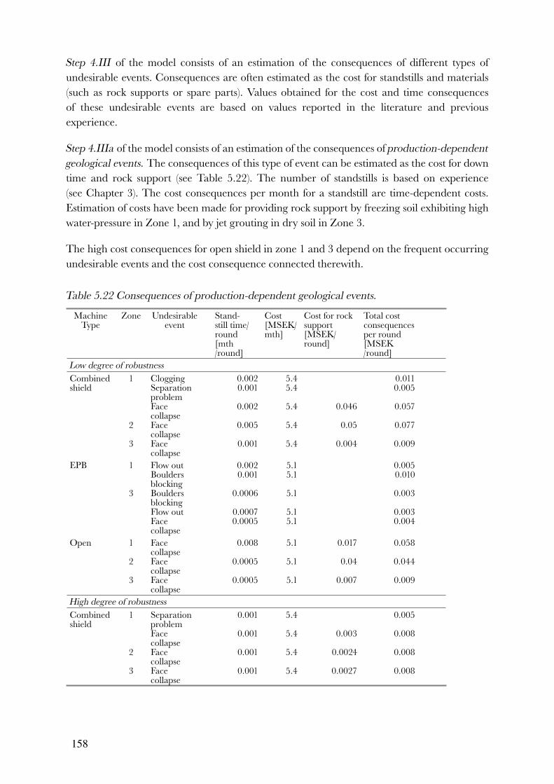
158

Step 4.III of the model consists of an estimation of the consequences of different types of undesirable events. Consequences are often estimated as the cost for standstills and materials (such as rock supports or spare parts). Values obtained for the cost and time consequences of these undesirable events are based on values reported in the literature and previous experience.

Step 4.IIIa of the model consists of an estimation of the consequences of production-dependent

geological events. The consequences of this type of event can be estimated as the cost for down time and rock support (see Table 5.22). The number of standstills is based on experience (see Chapter 3). The cost consequences per month for a standstill are time-dependent costs. Estimation of costs have been made for providing rock support by freezing soil exhibiting high water-pressure in Zone 1, and by jet grouting in dry soil in Zone 3.

The high cost consequences for open shield in zone 1 and 3 depend on the frequent occurring undesirable events and the cost consequence connected therewith.

Table 5.22 Consequences of production-dependent geological events.

MachineType

Zone Undesirable event

Stand-still time/round[mth/round]

Cost[MSEK/mth]

Cost for rock support[MSEK/ round]

Total cost consequencesper round[MSEK/round]


Combined shield

1

2

3

CloggingSeparation problemFace collapseFace collapseFace collapse

0.0020.001

0.002

0.005

0.001

5.45.4

5.4

5.4

5.4

0.046

0.05

0.004

0.0110.005

0.057

0.077

0.009

EPB 1

3

Flow outBoulders blockingBoulders blockingFlow outFace collapse

0.0020.001

0.0006

0.00070.0005

5.15.1

5.1

5.15.1

0.0050.010

0.003

0.0030.004

Open 1

2

3


0.008

0.0005

0.0005

5.1

5.1

5.1

0.017

0.04

0.007

0.058

0.044

0.009


Combined shield

1

2

3

Separation problemFace collapseFace collapseFace collapse

0.001

0.001

0.001

0.001

5.4

5.4

5.4

5.4

0.003

0.0024

0.0027

0.005

0.008

0.008

0.008

159

Table 5.22 continuation

MachineType


Stand-still time/round[mth/round]

Cost[MSEK/mth]

Cost for rock support[MSEK/ round]

Total cost consequencesper round[MSEK/round]

EPB 1

3

Boulders blockingFace collapseBoulders blocking

0.0001

0.00005

0.00005

5.1

5.1

5.1

0.00005

0.001

0.0001

0.0001

Open 1

2

3


0.003

0.001

0.001

5.1

5.1

5.1

0.017

0.000001

0.001

0.032

0.005

0.006

Step 4.IIIb of the model consists of an estimation of the consequences of randomly-occurring

geological events. The consequences of this type of event can be expressed as the cost due to down time and materials (see Table 5.23).

Table 5.23 Consequences of randomly-occurring geological events.

Machine type


No. of stand-stills

Standstill time[mth]

Total time[mth]

Cost[MSEK/mth]

Cost for materials[MSEK]

Total cost[MSEK]

Low/high robustness

Combined shield

3 Methane gas explosion

1 1 1 5.4 2 7.4

EPB 3 Methane gas explosion

1 1 1 5.1 2 7.1

Open 3 Methane gas explosion

1 1 1 5.1 2 7.1

Step 4.IIIc of the model consists of an estimation of the consequences of randomly-occurring

mechanical events. The consequences of this type of event can be estimated as the cost of down time and spare parts (see Table 5.24).

Table 5.24 Consequences of randomly-occurring mechanical events.

Machine type


No. ofstandstills

Standstill time [mth]

Cost[MSEK/mth]

Cost for spare parts[MSEK]

Total cost[MSEK]

Total time[mth]

Low/high robustness

Combined shield

All Failure of main bearing

1.0 0.5 5.4 0.5 3.2 0.5

EPB All Failure of main bearing

1.0 0.5 5.1 0.5 3.1 0.5

Open All Failure of main bearing

1.0 0.5 5.1 0.5 3.1 0.5

160

Step 4.IIId of the model consists of an estimation of the consequences of randomly-occurring

gross error. The consequences of this type of event can be estimated as the cost for down time and materials (see Table 5.25).

Table 5.25 Consequences of randomly-occurring gross error.

Machine type


No. of standstills

Standstill time[mth]

Cost[MSEK/mth]

Cost for material[MSEK]

Total cost[MSEK]

Low/high robustness

Combined shield

13

Over excavation

1 2 5.4 2 12.8

EPB 13

Over excavation

1 2 5.1 2 12.2

Open 13

Over excavation

1 2 5.1 2 12.2

Step 4.IV in the estimation model consists of an estimation of the exceptional cost or time for each type of event according to Equation 4.20. The total exceptional cost is estimated as the sum of the different types of events according to Equation 4.21. Table 5.26 shows the mean value and standard deviation of the exceptional time and cost for the different shield machines.

Table 5.26. Estimated total exceptional time [yr] and costs [MSEK]

Machine type Combined shield EPB shield Open shieldLow degree of

robustnessTime cost Time cost Time cost

Mean value 0.3 39 0.4 26 0.6 62

Standard deviation 0.2 7 0.1 5 0.8 58


Mean value 0.1 9.3 0.2 6 0.1 8

Standard deviation 0.1 13 0.1 10 0.1 13

In the following section the total time and cost will be estimated.

5.2.3 Total time and cost

Step 5 in the estimation model consists of a calculation of the total time or cost as the sum of normal time and cost plus exceptional time and cost for a certain tunnelling method over all the geotechnical zones according to Equation 4.22. Monte Carlo simulation is used to calculate the total time and cost. The number of Monte Carlo runs used in the estimation is 10,000 per simulation. The outcome of the estimation presents the total construction costs (and completion time) as a distribution curve. In order to be able to consider the impact of normal and exceptional time and cost and the degree of robustness, three different results are shown in the figures presented in this section. Normal construction time and cost, with a low degree of

161

robustness and partial correlation without considering exceptional time and cost is denoted by [1]. Total construction time and cost, with a low degree of robustness and partial correlation considering exceptional time and cost is denoted by [2]. Total construction time and cost with a high degree of robustness and partial correlation considering exceptional time and cost is denoted by [3]. Standard deviations for the results are calculated for partial and full correlation between the geotechnical characteristics. Standard deviation for full correlation has been estimated in the manner discussed in Step 3.Id. Figure 5.9 shows the result of a Monte Carlo simulation of the total construction time for the tunnel utilising different methods.

Figure 5.9 Result of simulations by shield machine type, where [1] is normal construction time

for a low degree of robustness and partial correlation without considering exceptional time; [2]

is the total construction time for a low degree of robustness and partial correlation considering

all exceptional time; and [3] is the total construction time for a high degree of robustness and

partial correlation considering all exceptional time.

Table 5.27 shows the mean values, as well as the standard deviation of the total construction times for the different tunnelling machines.

162

Table 5.27 Estimated total construction time [yr].



All exceptional time

Mean value 6.1 6.2 10.5

Standard deviation- partially correlated- fully correlated

0.41.2

0.30.9

0.92.2

Some exceptional time

Mean value 5.8 5.8 9.9

Standard deviation- partially correlated 0.3 0.3 0.5


All exceptional time


Standard deviation- partly correlated- fully correlated

0.20.6

0.31.1

0.83.1

Some exceptional time


Standard deviation -partially correlated 0.2 0.3 0.8

163

Figure 5.10 below shows the results of a Monte Carlo simulation of the total construction costs for the tunnel using different methods.

Figure 5.10 Results of the simulation by shield machine type in millions of Swedish kronor [MSEK], where [1] is the normal construction cost for a low degree of robustness and partial correlation without considering exceptional cost; [2] is the total construction cost for a low degree of robustness and partial correlation considering all exceptional costs; and [3] is the total construction cost for a high degree of robustness and partial correlation considering all exceptional costs.

164

The expected total construction cost and its variation depending on the degree of correlation between the geotechnical characteristics for the different machine types has been estimated and presented in Table 5.28.

Table 5.28 Estimated total construction costs by machine type [MSEK].


Low degree of robustnessAll exceptional costs [2]

Mean value 960 884 1130


3478

2361

73138

Some exceptional costs

Mean value 925 861 1070


3078

2584

45162


All exceptional costs [3]

Mean value 837 887 1056


2543

2971

57175

Some exceptional costs

Mean value 829 875 1051


2198

2884

56162

The analysis of the total construction time and cost for the different shield machines indicates that there are no major differences between the total construction costs for Combined and EPB shield. The combined shield, however, has a considerable lower construction time if high degree of robustness is applied compared to EPB shield. The reason might be that combined shield is better suitable for excavation both in soil under water pressure and in dry sandstone, which was present in the Grauholz tunnel project, especially if the reaches with high content of fines can be handled properly by a well- adapted separation plant. In the actual case, when constructing the Grauholz tunnel, the combined shield was used. The reason for the higher construction time using EPB shield is probably that the method is sensitive to boulders. This type of shield machine would probably be better if it was able to crush rocks. However, this is not possible with present-day technology. This method involves no separation. The total construction time as well as the cost for Open shield exceeds the combined as well as the EPB shield. The reason for that might be that the Open shield requires major drainage and support measures for excavation of large-diameter tunnels in soil under high water pressure. Thus, using this method entails very high costs. The analysis also shows that Open shield under the actual circumstances has a major uncertainty.

165

In the following section the actual time and costs are compared and discussed.

5.3 Comparison of estimated and actual time and costs

5.3.1 Introduction to the section

Geology

The geological conditions encountered were more complex than previously expected during the planning of the project. When tunnelling through the soil in Zones 1 and 3, the face support options able to used were affected for example by soil grain size distribution, cohesion and permeability. The soil in Zone 1 was especially problematic. The properties of the sandstone in Zone 2 were pretty well as expected. The pre-investigations of the soil section denoted West (Zone 3) revealed fines, but these originated from drilling dust. Due to the absence of fines in reality, it was necessary to use a slurry-supported face for the shield. No secondary separation was needed due to the lack of fines.

Tunnelling method

A combined shield machine was selected and used for excavating the Grauholz Tunnel. This machine type was considered to be the best choice for handling different geological zones. Table 5.29 shows some technical data for this machine.

Table 5.29 Technical data for the combined shield machine used in the Grauholz Tunnel.

Parameter Value

Cutter head - rotation speed [ r/m] 2.8

- numbers of front cutters [pcs] 65

- cutter diameter [cm] 42.5

- numbers of drag bits [pcs] 92

Power system

- installed pressure force [tonne] 10,000

- pressure in the working chamber [bar] 4

- pound length [m] 1.8

Separation system

- out-loading capacity [tonne/h] 450

- pumping capacity [m3/h] 1300

Electricity

- installed power [kW] 5600

- weight of shield [tonne] 500

Source: Balmer (1990)

The occurrence of boulders did not create any problems when using a combined shield. However, it would have been better to locate the stone crusher at the base rather than the centre of the bore head. There was no need for lowering the groundwater table in the soil section denoted East, as the face was supported by bentonite slurry.

166

Concrete segments were used to reinforce the tunnel. The size of each segment was 1.8 m in diameter x 5.8 m in length. This was the maximum size possible to handle, install and manufacture. In Zone 2, it would perhaps have been better to use a stiffer grout between segments and the ground. Further, a larger sealing profile (for example for the adjustment of erection error) on the segments would have been better. The durability of the lining is expected to be high.


The following two types of undesirable events actually occurred:

− collapse of the face (twice), and − settlements at the surface of the ground in the shape of craters (twice).

In Zone 1, the face collapsed during an attempt to enter the working chamber of the machine’s shield to change the cutters. Due to the high content of quartz—up to 45%—the wear and tear on the equipment was very high, leading to frequent cutter replacements. The collapse occurred when the bentonite slurry was pumped out, so that the upper part of the face was supported by overpressure. The reason for the collapse was a combination of the following factors:

− the thin layer of overburden (about 8 m), − partially cohesionless soil in layers, and − changing the face support from bentonite to air.

Over excavation when using overpressure in Zone 1 resulted in a crater with a diameter of 20 m and a depth of 2 m. After the collapse in Zone 1 it was clear that the stability of the face had to be reconsidered. Owing to the low face-stability and the collapse, work in the working chamber was not possible without taking some additional measures. As cutter changes would be required in the remaining soil section, it was necessary to find a method for enabling working at the face. The following alternatives were considered.

− Ground stabilisation from the aboveground surface via planned stations: this method had the advantage that changing the machine’s cutters could start immediately whenever a station was reached. However, the machine had to keep working until the next station was reached. Long boreholes for ground stabilisation (from the surface to the tunnel level) were required for this alternative.

− Ground stabilisation from within the tunnel: the disadvantage with this alternative was the long down time, as the stabilisation work could not be prepared in advance.

In Zone 1, freezing was used to stabilise the ground from the surface at planned stations. Due to a high level of wear on the cutters, it was necessary to change these every 50 m. Freezing was found to be the best alternative, considering the short construction time, the safety of the workers and environmental considerations. Due to cutter wear, the distance between the freezing stations varied. The freezing stations each consisted of a roof and a vertical wall,

167

covering the upper part of the face (see Figure 5.11).

The distance between the freezing pipes was 80 cm. For each freezing station, 15 vertical and 16 inclined pipes were needed. The frozen volume for each station was about 350 m2. The construction time of the stations including: boring boreholes with a total length of 520-690 m and installation of the piping system for liquid nitrogen was about 10 days. After changing the cutters—which could take anywhere from a few hours up to several days—the vertical pipes were removed from the ground and the tunnelling could continue. To build up and maintain freezing temperatures for the various elements during the repair work, approximately 1000 litres of liquid nitrogen were required per cubic metre of frozen soil.

Figure 5.11 Representation of the system for freezing via work stations at the Grauholz Tunnel; a lateral view and b looking head on, after Wenger (1994).

As the advance rate in Zone 1 was low due to the collapse, the tunnel schedule was delayed by about 13 months (corresponding to about SEK 80 million). Putting a freezing station in place in Zone 1 (drilling, installation and freezing) took 20 days and the cost was about SEK 1 million. Five stations were put in place for a cost of about SEK 6 million.

In Zone 3 a face collapse occurred, blocking the cutter head during an attempt to return to hydraulic support after changing the cutters. Stabilisation of soil was necessary in order to continue the excavation.

Grouting of stations was undertaken in zone 3 as the tunnel was located above the groundwater table. Each station consisted of 30 boreholes with a total length of 50 m (Wenger, 1994), and the grouted volume measured 14 m (wide) x 6.5 m (long) x 13 m (high), which can be seen in Figure 5.12. Grouting was performed in two steps; firstly with a concrete grout mixture, and secondly with silicate. In total, 12 m3 of concrete grout and 146 m3 of silicate were required for a theoretical soil volume of 1200 m3.

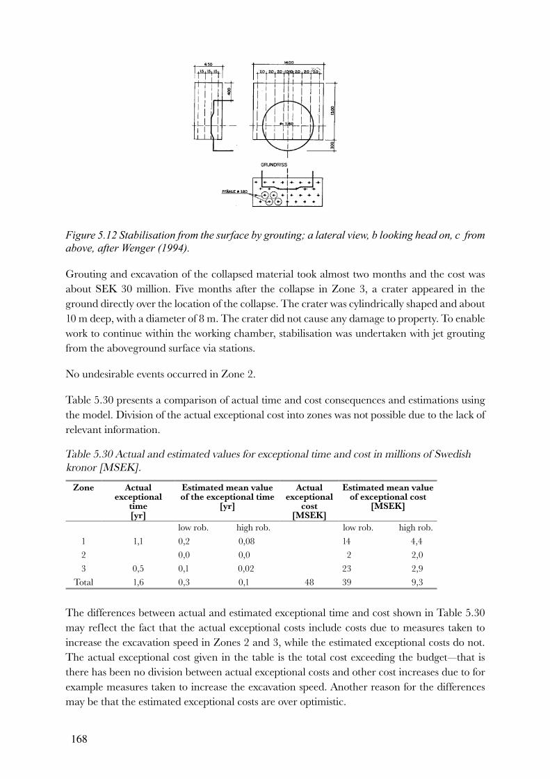
168

Figure 5.12 Stabilisation from the surface by grouting; a lateral view, b looking head on, c from above, after Wenger (1994).

Grouting and excavation of the collapsed material took almost two months and the cost was about SEK 30 million. Five months after the collapse in Zone 3, a crater appeared in the ground directly over the location of the collapse. The crater was cylindrically shaped and about 10 m deep, with a diameter of 8 m. The crater did not cause any damage to property. To enable work to continue within the working chamber, stabilisation was undertaken with jet grouting from the aboveground surface via stations.

No undesirable events occurred in Zone 2.

Table 5.30 presents a comparison of actual time and cost consequences and estimations using the model. Division of the actual exceptional cost into zones was not possible due to the lack of relevant information.

Table 5.30 Actual and estimated values for exceptional time and cost in millions of Swedish

kronor [MSEK].

Zone Actual exceptional

time [yr]

Estimated mean value of the exceptional time

[yr]

Actual exceptional

cost[MSEK]

Estimated mean value of exceptional cost

[MSEK]

low rob. high rob. low rob. high rob.

1 1,1 0,2 0,08 14 4,4

2 0,0 0,0 2 2,0

3 0,5 0,1 0,02 23 2,9

Total 1,6 0,3 0,1 48 39 9,3

The differences between actual and estimated exceptional time and cost shown in Table 5.30 may reflect the fact that the actual exceptional costs include costs due to measures taken to increase the excavation speed in Zones 2 and 3, while the estimated exceptional costs do not. The actual exceptional cost given in the table is the total cost exceeding the budget—that is there has been no division between actual exceptional costs and other cost increases due to for example measures taken to increase the excavation speed. Another reason for the differences may be that the estimated exceptional costs are over optimistic.

169

Robustness-increasing measures

Robustness-increasing measures were necessary for excavating through the complex geology. In order to determine what robustness-increasing measures to use, experience from other projects was used. Problems caused by the presence of boulders in the ground at the Hera Tunnel in Hamburg resulted for example in an integration of a stone crusher into the bore head. Some robustness-increasing measures for the shield machine used in the Hera Tunnel are listed below:

− a stone crusher in the middle of the bore head (to handle boulders), − a smooth wall in the working chamber (to handle high clay content), and − a jet pipe at the wall of the working chamber (to handle high clay content).

All these measures were applied on the combined shield from the start for the Grauholztunnel.

As the geology could not be predicted with sufficient accuracy, application of robustness increasing measures was also made during the construction. Data were continuously followed up to identify which measures that were necessary to apply.

As the geology cannot be predicted with adequate accuracy, application of robustness-increasing measures was also made during the actual construction phase. In order to estimate and eliminate causes for down time, the causes and the duration of periods of down time were noted throughout the entire construction period. Data were continuously followed up to identify weak points in the process. It was found that centrifuges were required to improve the separation process, and that a wear layer of the cutters were required to reduce the number of changes.

According to the geological pre-investigations, it was expected that Zone 3 would for the most part, consist of compact soil. Zone 3 was therefore planned to be excavated in dry mode—that is applying overpressure only. To increase the robustness of the method, it was decided however to start using a hydraulically-supported face. At the first attempt with only overpressure in the working chamber, great losses of air pressure occurred. The capacity of the compressor (200 m3/min overpressure) was insufficient due to the high permeability of the soil. It became therefore necessary to use additional material (saw dust) in the bentonite slurry to obtain a water tight filter cake on the soil surface.

The following measures were found necessary during construction:

− centrifuges instead of belt presses (to handle the high content of fines), − sawdust additives in the bentonite (to handle the low content of fines), and − wear coatings on the cutters (to reduce the number of changes).

The actual cost of taking additional taking measures to obtain a low degree of robustness (the stone crusher) was approximately 2% of the tender price. To obtain a high degree of robustness

170

(the centrifuges and wear coatings) cost approximately 4% of the tender price, and stabilisation of the soil to enable the safe change of cutters cost about 4.5%.

If the excavation had proceeded without any kind of robustness-increasing measures, then major problems such as the blocking of the bore head with boulders, and the clogging of the bore head throughout the whole length of Zone 1 would have occurred with a high degree of probability. Down time associated with each problem is between one to a number of weeks. This would result in a major delay compared with the planned construction time. Estimation of the total construction time without any robustness-increasing measures at all is therefore not done in this study.

5.3.3 Total construction time and cost

Total construction time

The actual advance rate in Zone 1 was only 3.5-4.5 metres per day (m/d), owing to major problems. In Zone 2, the advance rate was 15-17 m/d, and in Zone 3 it was 6.5-11.0 m/d. The lower advance rates include down time for collapses and rebuilding of the machine, which the higher values do not. The work was executed in two shifts of 10 hours per day (h/d) with 4 hours of maintenance per day. The capacity factor was not changed considerably after a longer period of excavation (learning period). Figure 5.13 shows the actual construction time, and construction time stated in the contract, estimated by the client and the contractor.

Figure 5.13 Planned construction time according to the contract and the actual construction time for the Grauholz Tunnel, after Aebersold (1994).

171

It can be stated that all additional equipment and robustness-increasing measures applied during the construction were profitable, as the time for completion (3.5 years) was not exceeded, and the budget came in within the expected frames.

The estimated and actual total construction times and costs have been compared for different zones along the tunnel in Table 5.31 below.

Table 5.31 Estimated and actual total construction times.

Zone Mean estimated time values [yr] Actual time

[yr]Low degree of robustness High degree of robustness

1 2.7 1.0 1.82 0.8 0.8 0.7

3 2.6 2.5 1.0

Total 6.1 4.3 3.5

From Table 5.31, it can be concluded that the actual time was generally lower than the one estimated with the model considering a low degree of robustness. This result is realistic, as robustness-increasing measures were applied. Considering a high degree of robustness, the estimated and actual time exhibit a lesser difference.

The reason for the differences in time between estimated and actual might be the measures to increase the capacity (such as increased amount of work hours per month) applied in zone 2 and 3 to keep the time frame. If no additional measures had been applied to increase the excavation speed, the actual and estimated speed would probably have exhibited less difference.

The total estimated construction time with a low degree of robustness was about six years, and with a high degree of robustness about four years. As measures to increase the excavation speed were applied during the construction period, the estimated construction time exceeded the actual time, which was about 3.5 years (Figure 5.14).

Figure 5.14 Comparison of actual and estimated construction time with exceptional cost, and

[1] a low degree of robustness, and [2] a high degree of robustness.

172

Total construction cost

The total construction costs were estimated for high and low degrees of robustness. Figure 5.15 shows the actual construction cost and estimated construction cost including all exceptional costs with low and high degrees of robustness for the tunnelling method. The reason why the actual construction cost exceeds the mean value of the estimated cost with a high degree of robustness may be that the robustness-increasing measures were applied after construction had already begun and not from the very start. Additionally, cost also occurred due to extra measures taken to increase the capacity of the method (to keep within the time frame). Based on the above, it can be concluded that the client could have used the model to estimate the budget in the planning stage.

Figure 5.15 Actual versus estimated total construction costs (in millions of Swedish kronor [MSEK]) with [1] a low degree of robustness and all exceptional costs, and [2] a high degree of robustness and all exceptional costs.

This analysis indicates that the decision to install high degree of robustness increasing measures should be taken in an early stage.

Figure 5.16 shows the actual construction cost and estimated construction cost including some exceptional cost with low and high degrees of robustness for the tunnelling method. The exceptional costs included in this case are costs that would fall under the responsibility of the contractor according to a unit price contract, such as the cost for a main bearing failure and clogging. The actual bid price from the contractor is slightly higher than the mean value of the cost estimated with the model considering a high degree of robustness. Based on the above, it can be concluded that the model would have been possible to use by the contractor to estimate the bid price in the tendering stage.

173

Figure 5.16 Actual versus estimated total construction costs in millions of Swedish kronor [MSEK] with [1] a low degree of robustness and some exceptional costs, and [2] a high degree of robustness and some exceptional costs.

This analysis indicates that the bidprice seems to be based on low degree of robustness and at the low side.

How factors like the degree of correlation and the type of cost to be considered affect the result of the estimation of time and cost using the estimation model are described in the following section.

5.4 Factors affecting the result of the Estimation of time and cost for combined shield

5.4.1 Degree of correlation

As discussed in Chapter 4, there is often correlation between the geotechnical characteristics. The degree of correlation, defined here as the distance within which the geotechnical characteristic show relatively strong correlation from one point to another, affects the distribution of total time and cost. Due to limited knowledge about the geotechnical characteristics, it is difficult to know which particular distance between correlated points should be considered, and which variation is the correct one to use in the estimation. The distance between correlated points is based on subjective estimation. Figures 5.17 and 5.18 show the distribution of normal construction time and cost for fully and partially correlated characteristics.

174

Figure 5.17 Normal time with [1] partially and [2] fully-correlated factors.

Figure 5.18 Normal cost in millions of Swedish kronor [MSEK] with [1] partially and [2] fully-correlated factors.

As shown in Figures 5.17 and 5.18, there is a major impact on the distribution depending on the distance between correlated points. The subjective choices in the estimations are therefore of major importance.

5.4.2 Type of costs considered

As discussed, there are different types of times and costs. Figure 5.19 shows the result of a Monte Carlo simulation of the total construction cost distribution considering different cost types. In this figure, the normal construction cost is shown without considering exceptional cost [1]. The same figure also shows construction cost including some exceptional cost [2], and also with all exceptional costs taken into consideration [3].

175

Figure 5.19 Results of the simulation in millions of Swedish kronor [MSEK] for [1] normal cost, [2] total costs taking some exceptional cost into account, and [3] total costs taking all exceptional costs into account.

This analysis indicates that different results can be obtained depending on the types of time and costs considered in the proposed estimation model. The difference between the mean values of the normal cost and the total cost including all exceptional costs is about 50 MSEK.

How factors such as the nature of the contract, project organisation, and the degree of robustness affect decision making is described in the following section.

5.5 Factors affecting decision making

5.5.1 Contract and organisation

As discussed in Chapter 2, there are different decision makers with different degrees of responsibility for increases in time and cost that may occur due to undesirable events. The client must determine the budget for the projects and the contractor the tender price. Clearly, the client has to consider dealing with the major part of all possible exceptional costs that may impact on the project, as it is the client who has the major responsibility. The contract and organisation of the project determine which sorts of exceptional costs will have to be considered by the contractor, as these factors determine which particular costs will be paid for by the client, should they occur. If the contractor has the minor responsibility, for example in a cost plus contract, then no exceptional cost need be considered (see [1] in Figure 5.20). The normal cost can therefore be basis for decisions about bidprice. Where there is some contractor responsibility, for example where the contractor has a unit price contract, then some of the exceptional cost should be considered by the contractor (see [2] in Figure 5.20). In this example [2] is when unit price contract is used, and the contractor has the responsibility for cost increases due to failure in machines and equipment, (cost for main bearing failure) and if the machine could not handle ground condition with high contents of fines which can cause clogging of the machine. Where the contractor has the major responsibility, for example a lump sum contract, then all the exceptional cost should be considered by the contractor. Often the client also has to take [3] into consideration when determine the budget (see [3] in Figure 5.20).

176

Figure 5.20 The distribution of costs in millions of Swedish kronor [MSEK] by contract type, where the contractor has: [1] a minor responsibility (e.g. a cost plus contract), [2] some responsibility (e.g. a unit price contract), and [3] the main responsibility (e.g. a lump sum contract) for the exceptional costs.

This analysis indicates that if the contractor has a low degree of responsibility, the cost range to consider in the decision process is much lower (about 80 MSEK) than if he has a major responsibility.

5.5.2 Degree of robustness

As discussed in Chapter 3, robustness-increasing measures may be used to increase the geological range within which the method may be used at normal or low production efforts. This means that the range of geotechnical characteristics where the method works with normal or low production efforts is extended. Applying robustness-increasing measures may result in increased normal cost and reduced exceptional cost, as the measures may decrease the sensitivity of the method and thereby reduce the consequences and probabilities of undesirable events occurring. Some measures can increase the method’s robustness much more than others. The degree of robustness affects how much the production effort required can be reduced, and the probability and consequences of undesirable events can be decreased, and thereby also how much the total construction time and cost can be reduced. These measures are profitable if the cost for these measures reduces the total time and cost by the same amount or more than when no measures are used. When tunnelling in what is considered to be “poor” ground and in complex geological conditions, there is normally a need for some additional measures to reduce the probability of extensive time and cost overruns. Figure 5.21 shows the total construction cost for a combined shield machine and additional robustness-increasing measures. Curve [2] in this figure represents using additional measures with a high degree of robustness—such as centrifuges in the separation process, and a separate centre cutter for handling a high clay content in the ground. Curve [1] in the same figure represents using additional measures with a low degree of robustness—such as the integration of a stone crusher to handle boulders. These measures increased the probability of achieving Production classes I and II and reduce the probability and/or consequence for undesirable events. The cost for the robustness increasing measures to obtain a high degree of robustness was in this case for combined shield about 10-15

177

MSEK. The measures resulted in a lower total cost of about 100 MSEK. As the application of measures to obtain a higher degree of robustness reduced the total construction cost more than they increased the cost they were in this case profitable.

Figure 5.21 Results of the simulation utilising additional robustness-increasing measures (in millions of Swedish kronor [MSEK]), where [2] represents a high degree of robustness, and [1] a low degree of robustness.

5.6 Conclusion

In this chapter, the estimation model described in this thesis has been applied to the Grauholz Tunnel in Switzerland. Based on this application, it can be concluded that the estimation steps described in Chapter 4 are clear and possible to follow. The separate estimation of normal and exceptional time and cost contribute to the clarity of the results. It has been shown that it is mainly the normal time and cost that impact on the construction time and cost, and that it is possible to estimate the exceptional time and costs for each identified undesirable event. This increases the possibilities available to the various parties (client and contractor) for using the results in different contractual and organisational situations.

Furthermore, it can be concluded that the results obtained from the estimation model are realistic. This is because the total construction time and cost obtained from the estimations correspond roughly to the actual construction time and cost. It may however, be difficult to compare actual and estimated time and cost, as different factors may be included in the actual results than in the estimated results. For example, costs due to additional measures taken to increase the excavation speed in reality, are not considered in the estimation. This may be one reason for the divergence seen between the actual and estimated time and cost values.

Due to the clear estimation of different factors affecting the result, a sensitivity analysis, can also be made with the proposed estimation model, i.e. which factors that have the major affect on the result can be estimated.

Application of the proposed estimation model shows also that the tunnelling method most suitable to the actual geological and hydrogeological conditions can be selected. This is possible as the normal cost as well as the exceptional cost that could be expected, are shown in the

178

result. Further, the application also shows that different degrees of robustness in the tunnelling methods are important considerations within the estimation, as the time and costs for these measures often increase the normal cost but reduce the normal time and exceptional time and cost. It has also been shown that the subjective estimation of the distance within which the geotechnical characteristics show relatively strong correlation from one point to another has a major affect on the degree of correlation, and therefore on the variation of the results.

179

6 Case study: the south marginal zone of the Halland ridge

tunnel project

6.1 Introduction

6.1.1 About the chapter

In this Chapter, the model for the estimation of time in tunnel projects described in Chapter 4 has been applied to a case study—the Halland Ridge Tunnel in Båstad, Sweden.

This chapter has the same aims as those already discussed in the Grauholz Tunnel case study presented in Chapter 5. However in this chapter, only time is considered and not costs. Another difference between the Grauholz Tunnel case study and this one, is that instead of studying the whole length of the tunnel as in the Grauholz Tunnel, only part of the tunnel has been studied here, being the South Marginal Zone.

This case study has been chosen in order to demonstrate the application of the estimation model to a well-defined project where a conventional tunnelling method was used.

6.1.2 Description of the project

The Halland Ridge Tunnel is 8.6 km in length. A 400 m long section running through a horst formation, and referred to as the South Margin Zone (SMZ), is the subject of this study. The SMZ was constructed in 1996-1997. The Halland Ridge bordering the southern Swedish counties of Skåne and Halland is one of the main obstacles for the West Coast Railway Line running between Gothenburg and Malmö. The ridge rises quite steeply to around 200 m above sea level and has created major problems for railway traffic since 1885, when the first part of this railway line was opened. In order to overcome these problems, two 8.6-kilometer-long tunnels with cross sections of 68-90 m2 (depending on rock quality) are currently under construction. Once fully completed and operational, the new twin-track rail link designed for high-speed trains will shorten travelling time between Gothenburg and Malmö by two some hours. Furthermore, the overall productivity of the rail link will be doubled.

The Halland Ridge Tunnel Project started in 1991, but due to technical and contractual problems relating to the use of a particular tunnel-boring machine, the first contractor aborted the project in May 1996, after completing only about 20% of the total tunnel length. Construction re-started in January 1996, when a new contract was signed by the client Banverket (the Swedish National Railway Administration—SNRA) and the contractor Skanska. A general contract was entered into by the client and contractor. The client (SNRA) was responsible for the design of all permanent structures, including permanent reinforcement, and the contractor (Skanska) was responsible for the design of the excavation method and the temporary reinforcement measures. In October 1997, the project came to a stop due to an undesirable and serious leakage of toxic substances into the tunnel surrounds, originating from a non-polymerised chemical grout. Groundwater close to the tunnel was contaminated as a result, and during the Swedish winter and spring of 1997, clean-up operations was undertaken. At the time of writing

180

this chapter, approximately 36% of the total tunnel length had been completed.

The rock along the length of the planned tunnel was classified according to the following parameters: rock type, degree of weathering, structure of rock mass, discontinuities and water characteristics, and the Q system (Koenigsberger ratio). The geological and hydrogeological conditions along the site are discussed in the following section.

6.1.3 Geology and hydrogeology

Step 1 of the model described earlier in the thesis consists of a determination of the geological and hydrogeological conditions along the tunnel’s planned alignment. The rock mass in the area of the Halland Ridge consists of Precambrian gneiss and amphibolite. The Halland Ridge is a horst formation resulting from major uplifting occurring approximately 100 million years ago. The rock mass within the horst is strongly affected by pronounced jointing and faulting, implying very complex geological conditions. The uplifting movement, caused severe fracturing and crushing on each side of the horst, today seen as the Northern and Southern Marginal Zones (NMZ and SMZ). These zones have also been subject to relatively strong deep weathering and parts of the rock mass have completely disintegrated into clay. Within the SMZ, Triassic sediments (mainly siltstones, claystones and unconsolidated sandstones) overlie the weathered basement rock. Within the confines of the horst, there is another major zone called Möllebäcken (the Mölle Stream) Zone. This zone differs from the marginal zones, exhibiting less weathering and extreme permeability. Figure 6.1 below shows a lengthwise geological section through the Halland Ridge.

Figure 6.1 Geological section along the length of the Halland Ridge Tunnel, after Sturk

(1998).

Due to the intense fracturing, the horst is completely saturated by water and the groundwater pressure at the tunnel level reaches 1.2 MPa. The ingress of water and sealing of the tunnels is one of the key issues within the project.

The SMZ is a zone of weakness of considerable size. The central part of the SMZ is affected by tectonic movements and weathering. Other parts are limited in their degree of disturbance. The SMZ is estimated to be 760 m wide. Comprehensive geological and hydrogeological investigations have been carried out in the SMZ on several occasions. Resistivity and seismic tests as well as core-drilling investigations have been undertaken and presented for example by

181

Dahlin et al. (1998). Based on these investigations, it could be stated that ravelling or running ground exhibiting short stand-up times (of less than 1 hour) are likely to occur in the area. Due to the extensive clay weathering, the rock mass is very weak in parts. The uniaxial compressive strength of the rock mass is in the range of 0.2-1 MPa in the weakest sections, which corresponds to “very stiff soil” or “very weak rock”. However within the weathered rock-mass, fresh cores stones are regularly encountered making the overall conditions relatively heterogeneous.

Step 2 of the model described in previous chapters consists of a division of the tunnel into distinct geotechnical zones exhibiting “homogeneous” geological conditions, and where the most appropriate tunnelling method for such conditions is chosen to suit the actual conditions found at the tunnel site. The length of tunnel studied here is defined by the chainage values 197+803 to 197+408 (km) in Figure 6.2 below.

Figure 6.2 Geological section along the length of the South Marginal Zone of the Halland

Ridge Tunnel, after Sturk (1998).

The SMZ has been divided into two main geotechnical zones based on the description of the geological conditions in Table 6.1.

182

Table 6.1 Length of the geotechnical zones in the South marginal Zone of the Halland Ridge

Tunnel.

Length[m]

Proportionate length of this part

of the tunnel[%]

Zone 1km 197+408 – 197+500km 197+593 – 197+743

92 150

24 35

Zone 2km 197+500 – 197+593km 197+743 – 197+803

93 60

25 16

Total 395 100

The decisions relating to rock support requirements were made according to the Q system (see Barton et al. 1974). The zones are therefore also divided up according to their predicted Q values. Zone 1 has a higher Q value than Zone 2.

The tunnelling method considered most suitable for the SMZ has been described in the next section.

6.1.4 Tunnelling methods

Step 2 of the model consists of selecting a tunnelling method most appropriate for the job given the actual geological and hydrogeological conditions, and project organisation. The tunnelling method planned for the SMZ was conventional (excavation) with drilling and blasting. The conventional method has been described in Chapter 3.

Due to the prediction of complicated geological conditions, it was stated that some form of robustness-increasing measures would be required to achieve safe and profitable excavation. In order to work out just what robustness-increasing measures ought to be used, experience from other projects was utilised. As only a minor amount of water inflow was expected in this part of the tunnel—due to the high degree of weathering and high clay content—spiling was chosen as the most suitable robustness-increasing measure.

In this study, spiling and pipe-umbrella robustness-increasing measures have been considered. The spiling in the study is assumed to have been undertaken using 6-8 m Swellex at a distance of approximately 0.5-1.0 m with 3 m overlapping. The pipe umbrella is assumed to have been constructed using 20 m steel piles at a distance of 35-40 cm and 3 m overlapping. The method considered in the estimations features temporary reinforcement with 30 cm thick shotcrete, reinforcement meshes and a face support of 5 cm thick shotcrete. Partial excavation producing a tunnel-round length of 1.2-1.5 m with a road header and hydraulic hammer (instead of blasting) has been considered in the estimation. Construction time for permanent reinforcement using shotcrete has not been considered in the estimation, as it was not on the critical time path.

If the excavation had been made without any kind of robustness-increasing measures, a reduced

183

round length of about 0.5-1 m would have been required. Despite the reduced round length and extensive rock support using shotcrete and bolting, repeated collapses would have occurred with a high degree of probability across the entire zone. The down time associated with each collapse ranges from one to several weeks. This would result in a major delay of the planned construction time. Estimation of the total construction time without any robustness-increasing measures has therefore not been made in this study.

The various robustness-increasing measures that can be used with conventional methods are described in more detail in Chapter 3. Estimation of the construction time featuring spiling and pipe umbrella techniques is discussed in the following section.

6.2 Estimation of time

6.2.1 Normal time

Step 3 of the model consists of an estimation of normal time and cost. In this study however, only normal time has been studied. Normal time is the time required for constructing the length of tunnel.

Step 3.I of the model consists of an estimation of the production effort required for the time component (Q

t) over the length of the zone (L).

Step 3.Ia of the model consists of a determination of the distribution of geotechnical characteristics that impact on the production effort for the tunnelling method being considered. The production effort for a conventional method using spiling or pipe umbrella techniques are affected by rock quality, clay content and water leakage. Table 6.2 shows the predicted values for the geotechnical characteristics rock quality, clay content and water leakage based on the geological pre-investigations. The estimated content of clay is based on the predicted degree of weathering. Rectangular distribution is used for the geotechnical characteristics (for the same reasons mentioned in Chapter 5).

Table 6.2 Predicted values of the geotechnical characteristics in the South marginal Zone of

the Halland Ridge Tunnel, according to Banverket (1995).

Geotechnical characteristic

Unit Zone 1Min. Max.

Zone 2Min. Max.

Rock quality Q value 0.01 0.1 0.1 2.0

Clay co ntent % 5 35 5 35

Water leakage L/(min. 100m) 10 150 10 150

Step 3.Ib of the model consists of a determination of the production classes within each zone and for each geotechnical characteristic—for example high, normal and low production efforts. In this case, three classes with high, normal and low production effort have been considered. The limits of geotechnical characteristics or groups of geotechnical characteristics corresponding to a change between production classes have also to be defined. In this study, these values

184

are called method-specific limits. Table 6.3 show the limits of the geotechnical characteristics of rock quality, clay content and water leakage for the methods studied. The values for these limits are based on interviews with for example, Lauffer (2001) and Kuhnhenn (1997), and are therefore subjective estimations.

Table 6.3 Estimated limits between different production classes for different geotechnical

characteristics and for different robustness-increasing measures, where A = rock quality [Q

value], B = clay content [%] and C = water leakage [l/(min 100m)].

Production class I II III

Spiling A

BC

0.1<A<2

>25<20

>20.01<A<0.1

20<B<2520<C<100

<0.01

<20>100

Pipe umbrellaA

BC

0.1<A<2

>25<20

>20.01<A<0.1

15<B<2520<C<100

<0.01

<15>100

Table 6.3 shows that a pipe umbrella can be used in lower clay content conditions than spiling can, and achieve Production class II.

Figures 6.3 to 6.5 illustrate the limits between the defined production classes for different geotechnical characteristics based on Table 6.3. The predicted ranges of the geotechnical characteristics shown in these figures is based on Table 6.2. Figure 6.3 illustrates the production classes for various rock qualities, Figure 6.4 for various clay contents, and Figure 6.5 for different degrees of water leakage.

Figure 6.3 Production class for spiling and pipe umbrella measures in various rock qualities.

185

Figure 6.4 Production class using spiling and pipe umbrella measures by clay content.

Figure 6.5 Production class for spiling and pipe umbrella measures by degree of water

leakage.

Step 3.Ic of the model consists of an estimation of the probability of each production class occurring. In the actual case, the geotechnical characteristics are assumed to affect the production effort like a “series” system (see Figure 6.6).

Figure 6.6 A series system where the geotechnical characteristics affect the production effort

of a conventional method.

186

The limits of each production class in Table 6.3 have been compared with the predicted range of values according to the results of the pre-investigation of the geotechnical characteristics in Table 6.2. Monte Carlo simulation has been used to estimate the probability for each production class according to Equations 4.37 to 4.43. Table 6.4 shows the results of the simulation. This table shows that the pipe umbrella technique has a higher probability of working normally under the given circumstances.

Table 6.4 Probabilities of achieving different production classes with a conventional

tunnelling method utilising various robustness-increasing measures.

Production class

Spiling Pipe umbrella

Zone 1

I 0 0

II 0.32 0.43

III 0.68 0.57

Zone 2

I 0.02 0

II 0.30 0.43

III 0.68 0.57

Step 3.Id of the model consists of an estimation of the production effort for the time component in each production class into the following: optimistic with the lowest expected production effort, probable production effort, and pessimistic with the highest expected production effort. The production effort is expressed as a stochastic variable with triangular distribution. As discussed earlier, the tunnelling process can be viewed as a cyclic process, consisting of various unit operations. The production effort can be expressed as the sum of the times for each unit operation in [h/m], (see Equation 5.1 below). The operations are assumed to be uncorrelated in the following:

(5.1)

where ti is the time expressed in hours for the different unit operations required for tunnelling

a distance (l) of one meter. The unit operations can include for example: drilling, loading, charging, ventilation activities, mucking out, temporary rock support, various episodes of down time such as due to the failure of a component or waiting for spare parts or geological surveying. The total time is estimated as fixed time during site “mobilisation and demobilisation” periods, and the time taken for the excavation. Table 6.5 show variables and constants for the estimation of the production effort for the time component. These values are based on experience from projects where conventional methods have been applied (for example the Rupertus and Umfahrung Melk projects).

Table 6.5 Constants used in the estimation of the production effort of the time component.

Description Unit Value

Working hours/day h/d 20Round length using spiling m 1.2

Round length using a pipe umbrella m 1.5

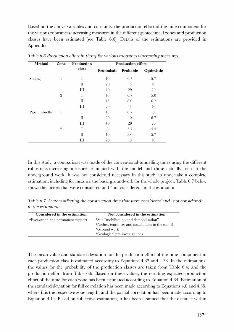
187

Based on the above variables and constants, the production effort of the time component for the various robustness-increasing measures in the different geotechnical zones and production classes have been estimated (see Table 6.6). Details of the estimations are provided in Appendix.

Table 6.6 Production effort in [h/m] for various robustness-increasing measures.

Method Zone Production

class

Production effort

Pessimistic Probable Optimistic

Spiling 1 I 10 6.7 5.7

II 20 13 10

III 40 29 20

2 I 10 6.7 5.0

II 13 8.0 6.7

III 20 13 10

Pipe umbrella 1 I 10 6.7 5

II 20 10 6.7

III 40 29 20

2 I 8 5.7 4.4

II 10 8.0 5.7

III 20 13 10

In this study, a comparison was made of the conventional-tunnelling times using the different robustness-increasing measures estimated with the model and those actually seen in the underground work. It was not considered necessary in this study to undertake a complete estimation, including for instance the basic groundwork for the whole project. Table 6.7 below shows the factors that were considered and “not considered” in the estimation.

Table 6.7 Factors affecting the construction time that were considered and “not considered”

in the estimations.

Considered in the estimation Not considered in the estimation

*Excavation and permanent support *Site “mobilisation and demobilisation”*Niches, entrances and installations in the tunnel*Ground work*Geological pre-investigations

The mean value and standard deviation for the production effort of the time component in each production class is estimated according to Equations 4.32 and 4.33. In the estimations, the values for the probability of the production classes are taken from Table 6.4, and the production effort from Table 6.6. Based on these values, the resulting expected production effort of the time for each zone has been estimated according to Equation 4.34. Estimation of the standard deviation for full correlation has been made according to Equations 4.8 and 4.35, where L is the respective zone length, and the partial correlation has been made according to Equation 4.15. Based on subjective estimation, it has been assumed that the distance within

188

which the geotechnical characteristics show relatively strong correlation from one point to another is 100 m, as this roughly corresponds to the zone length. Table 6.8 below shows the normal construction time for various robustness-increasing measures.

Table 6.8 Total normal construction time [yr] for various robustness-increasing measures.

Method Spiling Pipe umbrella

Zone1 2 tot.

Zone1 2 tot.

Mean value 1.0 0.4 1.4 1.0 0.3 1.3Standard deviation- partial correlation - full correlation

0.2 0.1 0.30.4 0.1 0.4

0.3 0.1 0.30.4 0.1 0.4

From Table 6.8 it can be concluded that construction time with spiling takes somewhat longer than with a pipe umbrella. The reason for this might be that the excavation process is less disturbed using a pipe umbrella than with spiling.

6.2.2 Exceptional time

Step 4 of the model consists of an estimation of exceptional time. Which particular ‘exceptional time’ ought to be considered in the estimation depends on the client or contractor’s responsibility arrangements (contractual and other project-related conditions). In this step, events causing exceptional time that fall within either the client or the contractor’s responsibilities are estimated.

Step 4.I of the model consists of an identification of undesirable events. Identification is based on experience gained from other projects with similar rock and soil conditions and tunnelling methods. Table 6.9 shows production-dependent geological events, randomly-occurring geological events, and gross errors that may occur using a conventional method combined with spiling and pipe umbrella techniques.

Table 6.9 Identification of possible undesirable events with conventional methods.

Method Production-dependent geological event

Randomly-occurring geological event

Gross error

Spiling

Rockfall Face collapse

Water inflow Shotcrete breakdown

Pipe umbrella

RockfallFace collapse

Water inflow Shotcrete breakdown

Rockfalls may occur where there is insufficient support. Water inflows may cause stability and excavation problems. In the extremely poor rock, water inflows may cause stability problems

189

such as flowing ground. In areas with better rock conditions, water inflows may cause problems for excavation, and may require grouting. Grouting may be difficult where the clay content is high. Gross errors such as shotcrete-breakdown may occur due to insufficiently washed rock or insufficient quality in the shotcrete.

The probability of occurrence and the consequences of the undesirable events identified have to be estimated.

Step 4.II of the model consists of an estimation of the probability of the identified undesirable events occurring, according to Equation 4.19.

Step 4.IIa of the model consists of an estimation of the probability of the identified production-

dependent geological events occurring. An example of such an event from this study is a rockfall. The probability of this type of event has been estimated as the probability of exceeding the limit of a geotechnical characteristic according to Equation 4.44. Table 6.10 shows the input data and estimated probability of failure with different robustness-increasing measures.

Table 6.10 Probability of production-dependent geological events with different robustness-

increasing measures.

Method Undesirable event Geotechnical characteristics

Rounds[no]

Limit[%]

Predicted[%]

p(failures/round)

Spiling RockfallFace collapse

Clay contentClay content

329329

2020

5-355-35

0.50.5

Pipe umbrella


Clay contentClay content

263263

1515

5-355-35

0.330.33

Step 4.IIb of the model consists of an estimation of the probability of the randomly-occurring

geological event identified. An example of such an event from this study is the occurrence of water-bearing zones. The probability of this event type occurring along a tunnel of reach L has been calculated according to Equation 4.46. Table 6.11 shows constants used in the calculation and the estimated probability of failure. The input data in the tables are based on subjective estimations and experience.

Table 6.11 Probability of randomly-occurring geological events.

Method Undesirable

event

Failure rate

[1/m]

Number of events

[p* ]

Spiling Occurrence of water-bearing zone 0.001 0.24

Pipe umbrella Occurrence of water-bearing zone 0.001 0.24

Step 4.IId of the model consists of an estimation of the probability of the randomly-occurring

gross error identified. An example of such an event from this study is the occurrence of a

190

shotcrete breakdown. The probability of this event type occurring is estimated based on subjective estimations and experience. It has been assumed that the probability of this type of failure is 0.25.

Step 4.III of the model consists of an estimation of the consequences of the different types of undesirable events. The consequences of these undesirable events are an increase in the production effort required and an increase in down time. An increase in production capacity for the remaining part of the tunnel is often necessary to maintain the planned construction schedule. Values for these time consequences are based on literature studies and experience.

Step 4.IIIa of the model consists of an estimation of the consequences of the identified production-dependent geological events. The consequences of this type of event are estimated as down time for mucking and additional rock support (see Table 6.12). The number of standstills is based on experience (see Chapter 3).

Step 4.IIIb of the model consists of an estimation of the consequences of the randomly-occurring

geological event identified. The consequence of this type of event is estimated as down time for pumping and grouting (see Table 6.12).

Step 4.IIId of the model consists of an estimation of the consequences of the randomly-

occurring gross error identified. The consequences of this type of event are estimated as down time (see Table 6.12).

Table 6.12 Consequences of various undesirable events.

Method Undesirable event Standstills

[no.]

Down

time/

no. of

standstills

[mth/no]

Total time

consequence

[mth]

Spiling RockfallFace collapseShotcrete breakdownWater-bearing zone

329329

50.24

0.0020.0040.251.0

0.661.321.3

0.24

Pipe umbrella

RockfallFace collapseShotcrete breakdownWater-bearing zone

263263

50.24

0.0020.0030.251.0

0.530.791.3

0.24

Step 4.IV of the estimation model consists of an estimation of the exceptional time for each type of event as the sum of the product of the probability and the consequences according to Equation 4.20 and 4.21. Table 6.13 shows the expected value of the total exceptional time.

191

Table 6.13 Estimated exceptional time [yr].

Method Event type Gross

error

Ce

time

[mth]Production-


event

Randomly-

occurring geological

event

SpilingRockfallFace collapse

0.0280.055

Water-bearing zone 0.02Shotcrete break-down

0.025

Total 0.125Pipeumbrella


0.0150.022

Water-bearing zone 0.02Shotcrete break-down

0.025

Total 0,08

Figure 6.7 shows the probability distribution of the exceptional time for spiling and pipe umbrella measures estimated using Monte Carlo simulation.

Figure 6.7 Exceptional time in years for spiling and pipe umbrella measures.

6.2.3 Total construction time

Step 5 in the estimation model consists of a calculation of the total time as the sum of normal time and exceptional time over all geotechnical zones according to Equation 4.22. Monte Carlo simulation is used to calculate the total time. The number of Monte Carlo runs used is

192

10,000 for each simulation. The outcome from the estimation shows the total construction time as a distribution curve. In order to be able to consider the impact of normal and exceptional time, two different results are shown in the figure presented in this section. The figure shows the normal construction time partially correlated without taking exceptional time into consideration [1], and the total construction time when exceptional time is considered [2]. The standard deviation of the result is calculated for partial and full correlation between the geotechnical characteristics. The standard deviation for full correlation has been estimated as discussed in Step 3.Id. Figure 6.8 shows the results of the Monte Carlo simulation of the total construction time for the SMZ for different robustness-increasing measures.

Figure 6.8 Result of the simulation of conventional methods with different robustness-

increasing measures, where [1] is the normal construction time with partial correlation without

considering exceptional time, and [2] the total construction time with partial correlation

considering all exceptional time.

In Table 6.14, the mean and standard deviation for partial correlation of the total construction times for the various robustness-increasing measures have been given.

Table6.14 Estimated total construction time [yr] with spiling and pipe umbrella measures.

Method Spiling Pipe umbrella

Mean value 1.6 1.4

Standard deviation - partially correlated- fully correlated

0.30.4

0.30.5

193

This analysis indicates that there are no major differences between the total construction time using spiling and pipe umbrella techniques. Both methods are suitable for excavation in highly-cohesive rock masses or stable rock, as was the case in the SMZ. Excavation using spiling as a robustness-increasing measure, however does not enable “large scale” excavation in a pre-prepared area, and is therefore not as safe as using a pipe umbrella (or jet grouting). Tunnel workers with experience from similar geological conditions of the actual conditions are required in order to achieve profitable excavation. The overlapping of the spiling required is almost 100%. This is time consuming and disturbs the excavation rhythm. A pipe umbrella requires less overlapping (about 15%). In cases where there are two parallel tunnels being excavated, the pipe installation work can be alternated with the excavation work.

In the following section, a comparison of the actual time and that estimated using the model is discussed.

6.3 Comparison of estimations with the actual results

6.3.1 Introduction to the section

Geology

The rock in the SMZ consists mainly of amphibolite and gneiss. As the rock in the crushed zones was relatively compact and contained clay, there was no problem with water as in other parts of the tunnel. Figure 6.9 illustrates the typical geological formations (after Sturk, 1998).

Figure 6.9 Geological section through the length of the Southern Marginal Zone of the Halland

Ridge Tunnel, after Sturk (1998).

The following features are identified in the above figure (after Sturk 1998).

a. The horst: on the north side of the depression, the marginal zone terminates and the horst—the uplifted rock block—begins; a transition from weathered to fresh permeable rock with high water flows is expected.

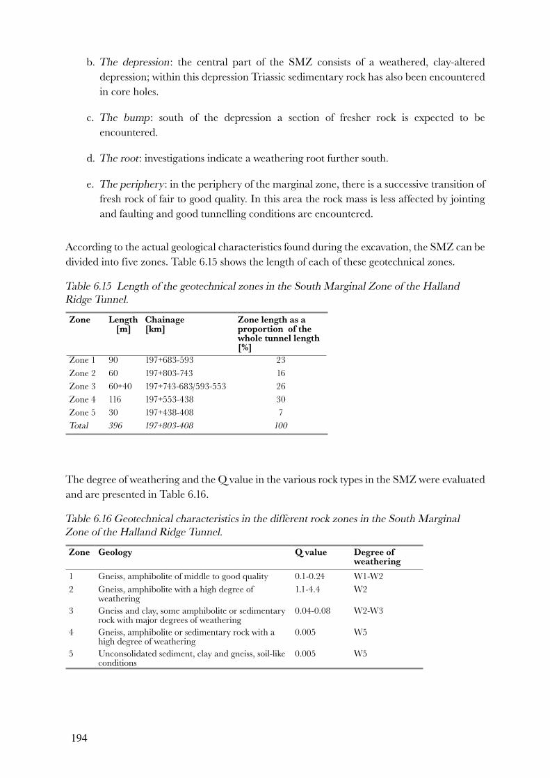
194

b. The depression: the central part of the SMZ consists of a weathered, clay-altered depression; within this depression Triassic sedimentary rock has also been encountered in core holes.

c. The bump: south of the depression a section of fresher rock is expected to be encountered.

d. The root: investigations indicate a weathering root further south.

e. The periphery: in the periphery of the marginal zone, there is a successive transition of fresh rock of fair to good quality. In this area the rock mass is less affected by jointing and faulting and good tunnelling conditions are encountered.

According to the actual geological characteristics found during the excavation, the SMZ can be divided into five zones. Table 6.15 shows the length of each of these geotechnical zones.

Table 6.15 Length of the geotechnical zones in the South Marginal Zone of the Halland

Ridge Tunnel.

Zone Length[m]

Chainage[km]

Zone length as a proportion of the whole tunnel length[%]

Zone 1 90 197+683-593 23

Zone 2 60 197+803-743 16

Zone 3 60+40 197+743-683/593-553 26

Zone 4 116 197+553-438 30

Zone 5 30 197+438-408 7

Total 396 197+803-408 100

The degree of weathering and the Q value in the various rock types in the SMZ were evaluated and are presented in Table 6.16.

Table 6.16 Geotechnical characteristics in the different rock zones in the South Marginal

Zone of the Halland Ridge Tunnel.

Zone Geology Q value Degree of weathering

1 Gneiss, amphibolite of middle to good quality 0.1-0.24 W1-W2

2 Gneiss, amphibolite with a high degree of weathering

1.1-4.4 W2

3 Gneiss and clay, some amphibolite or sedimentary rock with major degrees of weathering

0.04-0.08 W2-W3

4 Gneiss, amphibolite or sedimentary rock with a high degree of weathering

0.005 W5

5 Unconsolidated sediment, clay and gneiss, soil-like conditions

0.005 W5

195

Tunnelling method

A conventional method with spiling was chosen for the excavation of the SMZ in the Halland Ridge Tunnel. This method was considered best for handling the different geological conditions. Table 6.17 shows the excavation technique, round length and temporary reinforcement for each zone. The cross-section of the tunnel was 62-68 m2.

Table 6.17 Planned reinforcement for the different zones in the South Marginal Zone of the

Halland Ridge Tunnel.

Zone BoltingSwellex6 m

Shotcrete[cm]

Roundlength[m]

Excavation technique

Pre-bolting Spiling

1 Spot 5 4.6 Full face If required

2 Systematic 10 2.3 Full face Systematic Systematic

3 20 4.6 Heading/bench Systematic Systematic

4 Systematic 2.3 Heading/bench Systematic Systematic

5 25+5 1.0 Multiple drift Systematic Systematic

In Zone 1, continuous grouting was undertaken every 10 m. As there was a very low inflow of water, only a small amount of grouting material was required.

In Zone 2, draining of the water from the tunnel face in fault zones with a clay content was required. Long dewatering holes with a length of approximately 14 m were therefore drilled some metres behind the tunnel face. After the holes had dewatered the face, they were then grouted.

The systematic spiling was performed with reinforcement bars 7.5 m in length—Ks60s with a diameter of 26 or 32 mm. The distance between these was 0.3–1.0 m depending on the quality of the rock, and the angle of inclination has 5-15°. They were installed every second round in fault zones—that is every 2.3 or 4.6 m. The bolting was made using Swellex every metre; shotcrete arches with reinforcement meshes were placed every xm.

In Zone 3, the rock conditions were poor. After several rockfalls and problems with an unstable tunnel face, it was found necessary to excavate with heading and benching.

In Zone 5, the rock was very poor. The heading was therefore divided into several parts. A pilot tunnel was excavated in the middle of the face of approximately 4 x 4 m. A larger pilot tunnel was constructed in better rock conditions. After having blasted the pilot tunnel, the upper part was excavated with an excavator equipped with a jackhammer. In poor rock, a road header was used for the excavation, which gave a smoother surface. The tunnel face was reinforced with Swellex and shotcrete.

196

6.3.2 Normal time

In Zone 1, minor grouting was required, which resulted in a lower production effort being required than in other zones. In Zone 2, extensive grouting measures were required (approximately 50% of the working time). In Zones 3, 4 and 5, the time required for rock support accounted for about 60% of the total time, which is much more than in Zones 1 and 2. The production effort was higher than in Zones 1 and 2. Grouting accounted for 0-6% of the work time. Due to the poor geological conditions in Zone 5, the production effort was higher than in Zone 4. The down time was considerably higher than in the other zones due to for example media attention and medical examinations.

Standstills accounted for about 2-4% of the total construction time, and were caused by for example the following:

–repairing tunnel equipment (like a Bore Jumbo), –electrical installations, fans, and –miscellaneous (information and other meetings).

6.3.3 Exceptional time

During the excavation of the SMZ, the following types of undesirable events occurred:

–rockfall, –shotcrete failure, and –water inflow.

Rockfalls behind the tunnel face occurred repeatedly during the excavation. These incidents occurred as a result of reduced tension on the rock due to the high degree of weathering in the joints even where the general rock quality was good. An additional contributing factor was human error, due to a lack of adequate concentration during the shift changes and making incorrect interpretations of the rock conditions (the rock seemed to be better than it actual was). Some of the rockfalls were probably caused by the inflow of water.

Some of the rockfalls caused damage to tunnelling equipment and spiling. There were no accidents however resulting in injury to personnel due to the rockfalls, but clearly a major danger existed for the tunnel workers. The rockfalls caused delay due to the grouting that was required, and the additional reinforcement and excavation. The time consequences due to the rockfalls were relatively low. Each event caused a downtime lasting from hours to weeks. This resulted in a total downtime of about one month.

After the rockfall, it was stated that a more careful excavation with shorter round length (1.0-1.5 m) was necessary to achieve a reduction in the probability of repeated rockfalls occurring. It was deemed necessary to increase the diameter of the spiling to at least 32 mm and the bolting with radial Swellex to approximately 4 m, and the pre-bolts with an angle of 30o to about 7 m. It was also deemed necessary to increase the reinforcing of the tunnel face with shotcrete and

197

bolts and systematic dewatering holes. Optically checking for cracks in the shotcrete and for convergences in the tunnel was also deemed necessary.

Shotcrete breakdown occurred once. The rock in this area had a Q value of 1, the number of joints was about 20, and the degree of weathering about 2 at the time. The breakdown caused a delay of about one week, and was probably caused by a combination of the following factors:

–water pressure behind the shotcrete, –insufficient shotcrete quality, –insufficient washed rock, and –the contour in the heading being too rough.

In order to avoid this type of event, it was deemed necessary to wash the surface with water and sand before applying shotcrete, and to increase the degree of bolting, as well as to undertake more systematic visual checks after each excavation step.

Water inflow occurred in one of the tunnels when the parallel tunnel was being grouted. A water-bearing zone crossing both tunnels was probably the major cause of this incident. The zone probably contained crushed rock and continuous joints. Extensive grouting was required to reduce the water inflow.

A major collapse occurred at a chainage of 197+340 during excavation with a road header. The total amount of the collapsed rock material was about 300-400 m3. In order to continue with the excavation, a layer of crushed rock (gravel) and then shotcrete was placed in front of the collapsed material (see Figure 6.10). To further stabilise the material, a concrete base was cast and the material grouted. About 1000 m3 of cement grout was required for the stabilisation. Spiling and pre-bolting were also installed. However, due to other problems the tunnel work was shut down before the collapse occurred.

Figure 6.10 Collapse of the rock face at a chainage of 197+340 in the South Marginal Zone of

the Halland Ridge Tunnel.

198

6.3.4 Total construction time

It can be concluded that there were no major differences between actual and estimated total construction times (see Figure 6.11). The estimated mean value of the total estimated construction time with spiling was about 1.6 years and the actual time was 1.2 years.

Figure 6.11 Comparison of actual and estimated total construction time including exceptional

time for spiling

The actual tunnel advance rate was about 1.2 m/d. Work was executed in two shifts per day, each of 10.5 hours duration. Figure 6.12 shows the actual and planned construction time.

Figure 6.12 Planned and actual construction time for the South Marginal zone of the Halland

Ridge Tunnel according to the tunnel site.

From Figure 6.12, it can be concluded that the actual geotechnical characteristics were largely

199

within the limits where spiling works well. It was therefore possible to maintain the planned construction time.

How factors like the ‘degree of correlation’ and the ‘type of time considered’ affect the result of the estimation of time using the estimation model are described in the following section.

6.4 Factors affecting the results

6.4.1 Degree of correlation

As discussed in Chapter 4, there is often a correlation between the geotechnical characteristics. The degree of correlation—that is the distance within which the geotechnical characteristics show relatively strong correlation from one point to another—affects the distribution of the total time. Due to limited knowledge about the geotechnical characteristics, it is difficult to know which distance between correlated points to consider, and to know which variation is the correct one to use in the estimation. The distribution between correlated points is based on subjective estimation. Figure 6.13 shows the distribution of normal construction time for fully and partially-correlated characteristics.

Figure 6.13 Normal time with [1] partially-correlated factors, and [2] fully-correlated factors.

As shown by these figures, the distance between the correlated points determines whether the impact on the distribution is major or not. The subjective choices assumed in the estimation are therefore of major importance.

6.4.2 Type of time considered

As previously discussed, there are different types of times to consider. Figure 6.14 shows the result of a Monte Carlo simulation of the total construction time distribution considering different types of times. In the same figure, the normal construction time is shown without considering exceptional time, denoted by [1], and the construction time considering all exceptional time is denoted by [2].

200

Figure 6.14 Results of the Monte Carlo simulation using spiling: [1] the normal construction

time, and [2] construction time taking all exceptional time into account.

This analysis indicates that different results can be obtained depending on the types of time and costs considered in the proposed estimation model. In this study, the difference between the mean values of the normal time and the total time including all exceptional costs is about 2.5 months.

How factors like the particular contract and project organisation, and the degree of robustness affect decision making is described in the following section.

6.5 Factors affecting decision making

6.5.1 Contract and project organisation

As discussed in Chapter 2, there are different decision makers with varying degrees of responsibility for the increases in time (and cost) that may occur due to undesirable events. In Section 5.5.1, the affect of the apportioning of responsibility on which particular type of time ought to be considered in the decision-making process has been discussed. If the contractor has a minor responsibility (for example in a cost plus contract), the results from an estimation of normal time might be sufficient (denoted by [1] in Figure 6.15). If the contractor has a major responsibility however (for example a lump sum contract), the total time including all of the exceptional time might be required (denoted by [2] in Figure 6.15).

201

Figure 6.15 Distribution of total construction time depending on the apportioning of

responsibility, where the contractor has [1] partial responsibility, for example in a unit price

contract, and [2] major responsibility, for example in a lump sum contract.

This analysis indicates that where the contractor has a low degree of responsibility, the construction range to consider in the decision process is slightly lower (about 2.5 months) than where the constructor has a large degree of responsibility.

6.5.2 Robustness

As discussed in Chapter 3, robustness-increasing measures can be used to increase the geological range wherein the method can be used with a normal or low production effort being required. In Section 5.5.2, the affect of the degree of robustness on the total construction time (and cost) was discussed. Figure 6.16 shows the total construction time for the robustness-increasing measure spiling [1] and pipe umbrella [2]. As previous mentioned, repeated collapses would have occurred with a high degree of probability across the entire zone if no robustness increasing measures like spiling or pipe umbrella would have been applied. The down time associated with each collapse ranges from one to several weeks. This would result in a major delay of the planned construction time. Estimation of the total construction time without any robustness-increasing measures has therefore not been made in this study.

Figure 6.16 Results of the simulation of construction time with [1] robustness increasing

measure: spiling, and [2] robustness increasing measure: pipe umbrella.

202

6.6 Conclusion

In this chapter, the estimation model has been applied to the South Marginal Zone of the Halland Ridge Tunnel.

As discussed in the Conclusion in Chapter 5, it can be also be concluded here that the estimation steps described in Chapter 4 of the thesis are clear and able to be followed. The separate estimation of normal and exceptional time contributes to the clearness of the result. It has been shown that normal time has the biggest impact on the construction time, and that it is possible to estimate the exceptional time for each identified undesirable event, which increases the possibility for different parties (client and contractor) to use the results in different contractual and organisational situations.

Furthermore, it can be concluded that the results obtained from the estimation model are realistic, as the total construction time obtained from the estimations roughly corresponds to the actual construction time.

This application shows that the different degrees of robustness of the tunnelling methods chosen in this study do not impact on the results as much as they did in the other case study (see Chapter 5). It has also been shown that the subjective estimation of the distance between which the geotechnical characteristic show relatively strong correlation from one point to another have a major effect on the degree of correlation and therefore the variation of the results.

203

7 Summary and conclusion

7.1 Introduction

Generally, the client and the contractor decide budget and tender price respectively. However, both parties require access to an accurate representation of the distribution of total cost and time on which to base their decisions. Using an estimation model that provides an overview of the cost and time figures likely to arise during the construction of the project, can help improve the basis for making these decisions.

The demands facing such estimation model have been discussed in Chapter 2 of the thesis, and the characteristics of tunnelling methods and how these affect time and cost estimation has also been discussed in Chapter 3. The following subsections (7.1.1 and 7.1.2) summarise the main points from these two chapters.

7.1.1 Demands on estimation models for tunnel projects

It has been stated that tunnelling projects are sensitive to disturbances. The reason for is that the tunnelling process is a “serial” type production system in two senses. Firstly, in a serial setting the possibility for changing workplace location—in this case a tunnel—is limited, except when more than one tunnel adit is made. Secondly, the possibility for executing more than one main work activity at a time is also limited in tunnelling projects. Therefore disturbances often have a larger impact on time and cost in tunnelling projects than in other types of construction.

Various studies by for example Kastbjerg (1994), Andreossi (1998), and the HSE (1996) have shown that major cost and time overruns are common in infrastructure projects including tunnelling. As these overruns cause major problems for all the parties involved in the tunnelling process, it is important that the risk factors that may cause cost and time overruns be considered in a structured way in the estimation of cost and time for tunnelling projects.

Based on discussions about various risk factors and their impacts on cost and time values in tunnelling projects, it has been concluded that it is important to make a clear distinction between normal cost and time and the undesirable events that cause exceptional cost and time. Existing decision-aid estimation models, which handle variations in variables (such as the Successive method and the Decision Aids in Tunnelling) do not consider normal time or cost and undesirable events separately in the estimations.

Variation due to normal risk factors in this study are defined as “factors causing deviations in the normal time and cost span”. Examples of normal risk factors are performance-related factors like the advance rate of the tunnelling method.

In this study, undesirable events are defined as “events that cause major unplanned changes in the tunnelling process”. Undesirable events often occur due to physical factors like geological and hydrogeological conditions. Tunnel collapses and unexpected changes in geological conditions causing damage or a complete change of the excavation method are examples of undesirable events.

204

In this study, the term “robustness” is used to indicate flexibility and preparedness to deal with actual conditions. Based on case studies by for example Hentschel (1997), Wenger (1994), and Beck and Thullner (1998), it can be concluded that applying measures that increase the robustness of the tunnelling method affect the occurrence of undesirable events. Robustness must therefore be considered in the estimation.

Undesirable events caused by abnormal risk factors such as acts of God (earthquake, hurricanes and other natural calamities), cannot and should not be considered in the estimation of cost and time for a tunnel project. The consequences of abnormal risk factors are normally covered by insurance.

The construction contracting method as well as the stage of the project affect which of the parties (client or contractor) in the project is responsible for the increases in cost and time that may occur due to different risk factors (Kveldsvik & Aas,1998; Purrer, 1998; Eschenburg & Heiermann, 1998). Clearly, the client has the main responsibility for financing the project, however in some instances it may be appropriate for the contractor to pay for the cost of some of the risks. Variations in cost and time due to normal risk factors are often carried by the contractor, as normal risk factors fall mainly under the control of the contractor. Exceptional cost and time, due to undesirable-event-related risk factors are normally the responsibility of the client, who has the major financial strength. However in some cases, even exceptional cost and time is shared between the parties.

Estimations are normally made in a deterministic manner (Quellmetz, 1987). There is however, a need to be able to handle variation in cost and time variables in the estimation.

It can be concluded that an approximate calculation method would be best suited to handling variations in cost and time due to normal risk factors, as exact calculation methods either do not exist or are very complicated. From the approximate methods discussed, Monte Carlo simulation has been found to be most appropriate, as many uncertain correlated variables can be handled relatively easily. Undesirable events can be handled as discrete variables.

As the total cost of a tunnelling method is expressed as a distribution curve, the decision about which tunnelling method to use involves comparing their respective time and cost distributions. Based on these decisions, the budget and tender price have to be determined by the client and contractor respectively. Analysis methods and decision criteria that take into consideration these distributions are required for selecting an appropriate tunnelling method. Commonly used decision-analysis methods and criteria are often used for deciding between specific values. However there are other methods used for making decisions about tunnelling methods, tender prices and budgets. The main criteria used for decisions about which tunnelling method to use are not always the “minimum expected total cost and time”, but may also be for example, the probability of exceeding a certain value that is considered important to the decision.

205

7.1.2 Characteristics of tunnelling methods affecting the estimation of time and cost

The tunnelling method and the geotechnical characteristics are key considerations in estimating the time and cost for a tunnelling project.

The geological and hydrogeological conditions determine the most appropriate tunnelling method to use. Relatively few geological and hydrological parameters are required to make a preliminary choice. The large overlap in the method-viability ranges shows however that the final choice of tunnelling method is a complex process, where contractual and project-specific factors as well as economic, and environmental and safety aspects, all have to be considered.

Geotechnical characteristics also affect the productivity of the tunnelling method. The advance rates of different tunnelling methods in a range of different geological conditions have been described in the literature. It is important that the correlation between the advancerate of the tunnelling method and the geotechnical characteristics is taken into account in the estimation model.

The case studies discussed in Chapter 3 show that various types of undesirable events occur occasionally, and have consequences for each project in terms of time and cost. Some of the undesirable events that occur depend on the actual capacity of the method; others occur randomly due to the geological conditions encountered. There are also undesirable events that occur due to the failure of machinery or equipment. Gross human error is also the cause of some undesirable events. It is important to consider the impact of undesirable events on time and cost.

It has been concluded that robustness-increasing measures can be used to increase the geological range of a method’s application and rate of advancement. These can also reduce the probability of occurrence and the consequences of undesirable events. The most suitable robustness-increasing measures depend on the tunnelling method used. The effect of robustness-increasing measures on time and cost should be considered when estimating the time and cost of a tunnelling project.

The next section describes the theoretical estimation model and discusses the conclusions drawn about this model which takes the abovementioned demands into consideration.

7.2 Theoretical estimation model

It has been concluded that it is important for the client and contractor to have a good basis for making decisions about budgeting, tender pricing or selecting a tunnelling method at their disposal. Both parties need to be able to utilise the distribution of total time and cost as a basis for making decisions.

In order to respond to the demands placed on the basis for making decisions about tender price and budget, estimations can be made according to the five steps described in Chapter 4. The five main steps in the estimation model can be described as follows.

206

1. Determination of the geological and hydrogeological conditions along the

alignment of the tunnel.

2. Division of the tunnel into geotechnical zones with “homogeneous”

geological conditions and selecting a tunnelling method suited to the actual

conditions.

A geotechnical zone is defined as a “tunnel reach modelled as having similar geotechnical conditions, in which the one tunnelling method” is intended to be used.

3. Estimation of normal time and cost for each zone.

Normal time and cost is the time and cost for constructing the tunnel under normal circumstances. Normal time and cost are estimated in a similar way, independent of the partner in the tunnelling process (contractor or client), and the type of contractual and other conditions for the given project. In this estimation model, normal time estimations are based on the production effort of the method, and the normal cost is divided into three types of cost: time-dependent, quantity-dependent and fixed costs. The production effort is estimated for each type of cost as well as cost variables.

4. Estimation of exceptional time and cost for each zone

As discussed in Chapters 2 and 3, undesirable events of different types may occur and cause exceptional time and cost. Which particular exceptional time and cost ought to be considered in the estimation, depends on the client or contractor’s responsibility with regard to contractual and other conditions.

Five types of undesirable events have been identified: production-dependent geological events, randomly-occurring geological events, randomly-occurring mechanical events, gross errors, and miscellaneous events. Estimation of the exceptional cost or time for each event type is based on the consequences and probabilities expressed as distributions.

5. Calculation of the total time or cost using Monte Carlo simulation.

Total cost or time is expressed as the sum of normal time and cost, and exceptional time and cost for a given tunnelling method across all the geotechnical zones.

A separate estimation of normal and exceptional time and cost is made in the model. Exceptional time and cost is estimated for each identified undesirable event. This increases the possibilities available to the various parties (client and contractor) for using the results in a variety of contractual and organisational situations.

Normal and exceptional costs that could be expected in the particular project are then estimated using the model, for the different tunnelling methods and various geological and hydrogeological conditions. Various degrees of robustness in the different tunnelling methods can be considered in the estimation.

207

The estimation model developed has been applied to case studies. The conclusions drawn from this application are discussed in the following section.

7.3 Conclusion from application of the estimation model

The estimation model described in this thesis has been applied to the two case studies—the Grauholz Tunnel in Switzerland, and the Halland Ridge tunnel in Sweden.

It can be concluded that the results obtained from the estimation model are realistic. This is because the total construction time and cost obtained from the estimations roughly correspond to the actual construction time and cost.

The separate estimation of normal and exceptional time and cost contribute to the clearness of the result. It has been shown that the normal time and cost impact mostly on the construction time and cost, and that estimation of the exceptional time and costs for each undesirable event identified is possible. This helps to increase the possibility for different parties (client and contractor) to use the results in various contractual and organisational situations.

Due to the clear estimation of different factors affecting the results, a sensitivity analysis can also be performed on the proposed estimation model, revealing which factors have the greatest effects on the results.

Application of the proposed estimation model shows also that the tunnelling method most suitable for the actual geological and hydrogeological conditions can be selected using the model. This is possible, as the normal and the exceptional costs that could be expected are shown in the results. Furthermore, the application also shows that it is important to consider different degrees of robustness in the tunnelling methods, as the time and cost of applying these measures often increase the normal cost, but reduce the normal time and the exceptional time and cost.

The study has shown that it may be difficult to compare the actual and estimated time and cost in some cases. The reason is that different factors may be included in the actual results compared to the estimated results. For example, there may be actual costs for measures taken to increase the excavation speed that are not considered in the estimation. This may be one reason for the divergence between the actual and estimated time and cost.

209

8 Proposals for further research

The purpose of this thesis is to improve the quality of the basis used for making decisions about tender price and budgeting in tunnelling projects. Developing a model for the estimation of construction time and cost helps make this possible. As this model is new, there are many details that have only been discussed briefly. In some cases, rather rough assumptions have been made in order assist the development work move forward. Consequently, there is a lot of work to be done to further refine the model.

The following topics are suggestions to focus on in further research:

−the input data for the model, −the relationships between the variables, −the degree of robustness of the tunnelling method, −the relationship between the production effort and the geological conditions, −analysis of the construction process, −inventory control, −the impact of contracts and insurance on decision making, and −applying the estimation model to the financial market.

Input data for the model

A large amount of input data is required for estimating the total construction time and costs using the model. To obtain suitable input data for normal and exceptional time and costs, a database containing for example the undesirable events that occurred, and advance rates obtained under different geological conditions and tunnelling methods is required.

Relationships between the variables

The relationships between variables used in the model, such as the time required for executing various unit work operations, have been handled as uncorrelated variables. In order to study how changes in a particular variable influence the total result, it is also important to consider the correlation structure.

Degrees of robustness in the method

In this study, the term robustness has been used to express flexibility and preparedness to handle the actual conditions encountered. Based on case studies by for example Hentschel (1997), Wenger (1994), and Beck and Thullner (1998), it can be concluded that the application of measures that increase the robustness of the tunnelling method, affect the range of geological conditions in which the tunnelling method can be used, as well as the probability and consequences of the undesirable events. The optimal degree of robustness of the tunnelling method depends on many factors, including for example how much a change in the degree of robustness affects the geological-condition limits within which the method works well, as well as the cost of the measures. Therefore it is important to consider varying degrees of robustness in the estimation of time and cost for a tunnelling project.

210

Relationship between the production effort and the geological conditions

The production effort of a tunnelling method has a major impact on the total construction time and cost. The production effort is influenced by amongst other things, the actual geological conditions encountered. The geological conditions often show large variation and knowledge about them is limited. An important part of the estimation model is therefore knowledge about the relationship between the geological conditions and the production effort of the tunnelling method.

Analysis of the construction process

The tunnelling process is characterised as a “series” system in two senses of the word. Firstly, the possibility for changing the location of the workplace (in this case a tunnel) is limited, except when more than one tunnel adit is being constructed. Secondly, the possibility of executing more than one main work activity at a time is also limited. Disturbances often therefore have a greater impact on time and cost in tunnelling projects than in other types of construction projects.

When analysing the time required for different work activities, it can be stated that a major part of this time is down time due to disturbances. Identifying and minimising the causes of down time are therefore important. One step to achieve this is to make a disturbance analysis. The purpose of this analysis is to:

− identify how productivity varies due to disturbances in normal productivity; − increase the understanding of how the disturbances influence the process; and − identify the connections between robustness-increasing measures and disturbances.

A series-type system can be analysed using system-analysis methods such as queue theory.

Inventory control

The amount invested in inventory often exceeds the amount of capital invested in fixed installations and civil structures. By developing effective control of the inventory or administration of materials on construction sites, a reduction in the amount of capital sunk into “inventory” can be obtained. Methods and models that can be used to develop effective control of inventory have been discussed in the literature by for example Axsäter (1991) and Sherbrooke (1992). Most of these models and methods however, are concerned about permanent inventory rather than temporary inventory for single projects. There is a need however, for some kind of control of inventory for project-specific construction sites. The “Just in Time” approach already being practiced on certain construction sites, could be an example of this.

The impact of contracts and insurance on decision-making

It is important to use a basis for making decisions that is relevant to the apportioning of responsibility between the parties (client and contractor) concerned. It is important to analyse the influence that insurance and the type of contract used by the parties has on which particular

211

time and costs for risks should be included in the basis for making project decisions.

Application of the estimation model on the financial market

Application of a modified version of the estimation model related to decision about investments and targeting operations. The input is acquired from predictions of coming market trends and mass psychological behaviour within the financial markets.

213

REFERENCES

Aebersold, W, 1994: “Betrieb und erzielte Leistung mit dem Mixschild” Referate der Studientagung vom 26. Mai 1994 in Schönbühl, Fachgruppe für Untertagebau, SIA Dokumentation D0116, Grauholztunnel II (In German).

Aebersold, W, 1997 personal communication

Alén, C. 1998: ”On Probability in Geotechnics - Random calculation models exemplified on slope stability analysis and ground-superstructure interaction” Chalmers University of Technology, Göteborg, Sweden

Alén, C., 1996:”β-metoden” Sannolik geoteknik, Temadag SGF, 19 November, Chalmers, Göteborg (In Swedish).

Anagnostou, G., Kovári, K, 1994:” The face Stability of Slurry-shield-driven Tunnels” Tunnelling and Underground Space Technology, Volume 9, No 2.

Anagnostou, G., Kovári, K, 1996:” Face Stability Conditions with Earth-Pressure-Balanced Shields” Tunnelling and Underground Space Technology, Volume 11, No 2.

Anderson, J.M., 1997:” World-wide research points to the need for new approaches to control tunnelling risks” International Conference: Tunnelling under difficult conditions and Rock Mass classification, 27-29 Oct, Basel, Switzerland.

Anderson, J.M., Terezopoulos, N.G., 1997, :” The importance of education in the control of risks in tunnelling” Tunnelling under Difficult Conditions, Basel, Switzerland, October, proc pp 297-303.

Andreossi, E. M. 1998: ”Assessing underground tunnelling projects past and future role of reinsurers” Proc. Reducing risk in tunnel design and construction, 7-8 December, Basel, Switzerland, Independent Technical Conferences Ltd, Bredford, UK.

Ang, A. H-S, Tang, W.H., 1975: ”Probability Concepts in Engineering Planning and Design Volume I- Decision, Risk and Reliability” John Wiley & Sons, New York.

Ang, A. H-S, Tang, W.H., 1984:” Probability Concepts in Engineering Planning and Design Volume II- Decision, Risk and Reliability” John Wiley & Sons, New York.

Arz, P. Schmidt G H, Seitz, J, Semprich, S, 1991: ”Grundbau” Sonderdruck aus dem Beton-Kalender 1991, pp 43-44, 170-176 Bilfinger + Berger Bau AG (In German).

Axsäter, S., 1991:” Lagerstyrning” Transportforskningen, Studentlitteratur, Lund, Sverige (In Swedish).

Babendererde,S, 1991: ”Kritische Betraachtungen zum Einsatz von Hydroschilden”, Sicherheit und Risiken bei Untertagebauwerken, ETH- Symposium, 21/22 März 1991 (In German).

214

Baecher, G.B., Lanney, N.A., Einstein, H.H., 1977 „Statistical description of rock properties and sampling“ Proc. of 18th US Symposium on Rock Mechanics, 5C1-1 to 5C1-8.

Balmer, P, 1990: ”Die realisierte Lösung” Referate der Studientagung vom 23. August 1990 in Schönbühl Fachgruppe für Untertagebau, SIA Dokumentation D063, Grauholztunnel (In German).

Banverket, 1996: “Tender documentation, upphandling VKB U31/95, Skottorp-Förslöv New Railway Tunnels through Hallandsridge” Banverket Södra regionen, Malmö (In Swedish).

Barton, N., 2001: “Are tunnels faster by TBM?“ Tunnels and Tunnelling International, June 2001.

Barton, N., Lien, R., Lunde, J., 1974: ”Engineering Classification of Rock Masses for the Design of Tunnel support” Rockmechanics, Vol. 6, pp. 189-236.

Bartsch, M, 1995: ”Safety analysis of Swedish Dams. Dam Performance and Incident Data Analysis” Licentiate Thesis, Division of Hydraulic Engineering, Department of Civil and Environmental Engineering, Royal Institute of Technology, Stockholm, TRITA-AMI LIC 2005.

Bauer, F. 1999: ”Semmering-Basistunnel - Bestandsaufnahme und Realisierungskonzept” Felsbau 17 nr 5 (In German).

Beck, D., Thullner, T., 1998: ” Der Engelbergbasistunnel und der Umbau des Autobahndreiecks Leonberg” Tiefbau 10/1998 (In German).

Becker, C, 1990: ”Der Mixschild”Referate der Studientagung vom 23. August 1990 in Schönbühl Fachgruppe für Untertagebau, SIA Dokumentation D063, Grauholztunnel (In German).

Beitnes, A., Skjerdingstad, S., Undseth, E., 1995: ”Soft soil tunnel Eidsvoll-State of progress”.

Bell, E. Raiffa, H. Tversky, A. 1988: ”Decision making, Descriptive, normative, and prescriptive interactions” Cambridge university press, Cambridge.

Benjamin, J R, and Cornell, C.A, 1970:” Probability, Statistics and Decision for Civil Engineers” McGraw-Hill, New York, N.Y. 684pp.

Bienawski, Z.T. 1989: “Engineering rock mass classification” John Wiley & Sons, New York

Borg, L. 1999 spokesman for the Successive method in Sweden - private communication

Braach, O, 1994:” Extrudierbetonbauweise für Tunnelauskleidungen” Taschenbuch für den Tunnelbau, Verlag Glückauf GmbH, Essen (In German).

215

Brasser, J, 1990:” Die Methangasproblematik” Referate der Studientagung vom 23. August 1990 in Schönbühl Fachgruppe für Untertagebau, SIA Dokumentation D063, Grauholztunnel (In German).

Brox, D., Hagedorn, H., 1999: ”Extreme Deformation and Damage during the construction of Large Tunnels” Tunnelling and Underground Space Technology, Vol 14, No 1, pp 23-28.

Bruland, A. 1999: “Prediction model for performance and costs (of hard rock tunnel Boring)” Norwegian TBM tunnelling, Norwegian Tunnelling Society, NFF, 29-34, Oslo 1999. ISBN 82-991952-1-7

Bunner, J., Råsled, B., Söderberg, E., 1981: ”Byggstyrning-begrepp” Ekonomi och förvaltning, Handboken Bygg, Liber Förlag (In Swedish).

Chapman, C.B., Cooper, D.F., Cammaert, A.B. 1981: ”Model and situation specific or methods: risk engineering reliability analysis of an ing. facility” XIII- TIMS/LURO-III, Athens, July, 1977.

Charoenngam, C., Yeh, C-Y., 1999: ”Contractual risk and liability sharing in hydropower construction” International Journal of Project Management, Vol 17, No 1, pp 29-37.

Chauhan, R.L., 1998: “Impact of Management on Tunnel Advance Rates” Intern. Conf. On Hydropower Development in Himalayas, 1998, Shimla, India.

Chiaverio, F., Einstein, H.H, Köppel, U., 1995:” Risikoanalyse beim Adlertunnel” Schweizericher Ingenieur und Architekt, 4, 19. Jan. 1995.

Danielson, U., 1975: ”Produktionskalkylen - Byggarnas Resursadministration” Williamsson Offsettryck AB, Stockholm 1975 (In Swedish).

DAUB, Deutscher Ausschuβ für Unterirdisches Bauen, 1997:” Recommendations for Selecting and evaluating tunnel boring machines” Tunnel No 5/97.

Diewald, M., Wolff, V. 1997: „Semmering Basistunnel- Pilotstollen” Porr Nachrichten No 125, Allgem. Bau Porr AG, Austria.

Drees, G., Bahner, A., 1992: ”Kalkulation von Baupreisen, 3. neubearbeitete Auflage” Bauverlag GmbH, Wiesbaden und Berlin (In German).

Einstein, H.H., Dudt, J.-P., Halabe, V.B., Descoeudres, F., 1996:” Geologic uncertainities in Tunnelling”, Proc., Uncertainty in the Geologic Environment: from Theory to Practice.

Einstein, H.H, Salazar, G.F., Kim, Y.W., Ioannou, P.G., 1987:” Computer Based Decision Support Systems for Underground Construction”, Proc., RETC, Ch. 77, pp. 1287-1307.

216

Einstein, H.H, Descoeudres, F., Dudt, J.P., Halabe, V., Oktober 1991:” Entscheidungshilfen für den Tunnelbau”, Schlussbericht über die im Auftrag des Bundesamtes für Verkehr ausgeführten Arbeiten (In German).

Einstein, H.H. and Vick, S.G, 1974:” Geological model for a tunnel cost model” Proc. Rapid Excavation and Tunneling Conf., 2nd, II:1701-1720.

Eschenburg K-D., Heiermann W., 1998: ”Verteilung des Baugrundrisikos bei funktioneler Leistungsbeschreibung” Felsbau 16, nr 5 (In German).

Gehring, K. 1995: “Leistungs- und Verschleissprognosen im maschinellen Tunnelbau” Felsbau No 6/95, pp 439-448.

Gehring, K., Kogler, P, 1997:” Mechanized tunnelling: where it stands and where it has to proceed from a manufacturers view point” Tunnels for People, Golser, Hinkel & Schubert (eds), Balkema, Rotterdam.

Girmscheid, G, 1997:” Schildvortriebener Tunnelbau in Heterogenem Lockergestein, ausgekleidet mittels Stahlbetontübbingen Teil 1: Geophysikalische Baugrunderkundungsmethoden” Ernst & Sohn, Bautechnik 74 (1997), Heft 1 (In German).

Girmscheid, G.2000: “Baubetrieb und Bauverfahren im Tunnelbau” Ernst & Son Verlag GmbH, Berlin.

Gordon, M., 1994: ”Choosing Appropriate Construction Contracting Method” Journal of Construction Engineering, Vol 120, No 1, March 1994.

Hahn G.J., Shapiro S.S. 1967: “ Statistical Models in Engineering” Wiley, New York.

Haimes, Y.Y. 1998: ”Risk modeling, assessment and management” John Wiley & Sons, Inc.

Harr, M. E., 1987: ”Reliability-Based design in Civil Engineering” McGraw-Hill Company, New York.

Harsch, W., 1990:” Geologie und Hydrogeologie des Grauholztunnels” Referate der Studientagung vom 23. August 1990 in Schönbühl Fachgruppe für Untertagebau, SIA Dokumentation D063, Grauholztunnel (In German).

Harsch, W, 1994: ”Geologische Prognose und Wirklichkeit des Grauholztunnels” Referate der Studientagung vom 26. Mai 1994 in Schönbühl Fachgruppe für Untertagebau, SIA Dokumentation D0116, Grauholztunnel II (In German).

Hartman, F., Snelgrove, P., 1996: ”Risk Allocation in Lump-Sum Contracts - Concept of Latent Dispute” Journal of construction engineering and management, september 1996.

Health and Safety Executive, 1996:” Safety of New Austrian Tunnelling Method tunnels - a review of sprayed concrete lined tunnels with particular reference to London Clay” HSE Books 1996, 86pp.

217

Health and Safety Executive 1993: ”The cost of accidents at work” HSE Books, Sudbury, Suffolk

Henley, E.J., Kumamoto, H. 1981: “Reliability engineering and risk assessment” Prentice-Hall, Englewood Cliffs, N.J.

Hentschel, H. 1997: ”Difficult Start to Adler Tunnel” Tunnel Nr 1/97.

Hillier,S, Lieberman,G.J, 1995: ”Introduction to operations research” Mc Graw-Hill Book Co, Singapore.

Hintze, S, 1994:” Risk Analysis in Foundation Engineering with Application o Piling in Loose Friction Soils in Urban Situations” Doctoral Thesis, Division of Soil and Rock Mechanics, Stockholm, Sweden.

Hoek, E. Brown, E.T., 1980: “Underground Excavations in Rock” The Institution of Mining and Metallurgy, London.

Inokuma, A., Suzuki, S., Maruyama, I., Mitsuo, J., Sakai, T., Tokunga, Y., 1994: ”Studies on the present state and the mechanism of trouble occurrence in tunnel construction in Japan” Tunnelling and Ground Conditions, Abdel Salam (ed.), Balkema, Rotterdam.

Isaksson, M., Lindblad, M., 1997:” Störningsorsaker vid tunneldrivning - Fallstudie Siebergtunneln” Examensarbete vid avd. för Jord- och Bergmekanik, inst. För Anläggning och Miljö, Kungl. Tekniska Högskolan (In Swedish).

Isaksson, T. 1996:” Erfarenheter från tunneldrivning i jord och dåligt berg med mixsköld och jetgrouting” SveBeFo Rapport 25 (In Swedish).

Isaksson, T. 1998a: ”Tunnelling in poor ground - Choice of shield method based on reliability” Geotechnical Hazards, Pore´c, Croatia.

Isaksson, T. 1998b: ”Tunneldrivning med sköld - riskbaserad beslutsmodell” Licentiate Thesis 2030, Division of Soil and Rock Mechanics, Dep. of Civil and Environmental Engineering, Royal Institute of Technology, Sweden (In Swedish)

Isaksson, T., Reilly, J., Anderson, J., 1999a: ”Risk mitigation for tunnelling projects - a structured approach” Challenges for the 21st Century, ITA Oslo, Norway

Isaksson, T., Reilly, J., Anderson, J., 1999b: ”Mit Risikoanalyse und Innovativer Projektsteuerung Kostenbewuβt Bauen” Unterirdisches Bauen 2000 - Herausforderungen und Entwicklungspotentiale, STUVA-Tagung in Frankfurt, Germany

ITA, 1988: ”Recommendations on contractual sharing of risks” Tunnelling & Underground Space Technology, Vol 3/2 1988.

Jancsez, S., Steiner, W., 1994:” Face support for large Mix-shield in heterogeneous ground conditions” Tunnelling -94, London.

218

John, M., Wogrin, J., Heiβel, G. 1987: ”Analyse des Verbruches im Landrückentunnel, Baulos Mitte” Felsbau 5 (1987) Nr.2 (In German).

Kapur, K.C., Lamberson, L.R. 1987: “Reliability in engineering designs” Wiley, New York.

Kasa, H, Yamamori, T., Nishida, S., Ohga, K. 1994: ”Experimental studies on monitoring obstacles in front of a shield tunnelling machine using an acoustic wave and Rayleigh wave” Hazama News, Japan.

Kastbjerg Skamris, M. 1994: ”Large Transport Projects - Forecast versus Actual Traffic and Costs” Master’s Thesis in International Technology Planning, Aalborg University, Denmark.

Kleivan, E., Berdal, A.B. 1991 “NoTCoS-Norwegian Tunnelling Contract System” Norwegian Tunnelling Today, Norwegian Soil and Rock Engineering Association, Publication No 5, Tapir Publishers

Kovári, K, 1985:” Probleme der Gebirgsverformungen bei der Anwendung von Vollvortriebsmaschinen im Fels” SIA-Dokumentation 91, Tunnel und Stollenbau im Fels mit Vollvortriebsmaschinen (In German).

Kovári, K, Fechtig, R, Amstad, Ch, 1991:” Erfahrungen mit Vortriebsmaschinen grossen Durchmessers in der Schweiz” STUVA-Tagung, Düsseldorf (In German).

Kuhnhenn, K, 1995:” The New Austrian Tunnelling Method” article in Tiefbau edition 5/95 pages 20-29.

Kuhnhenn, K, 1997 private comunication

Kveldsvik, V., Aas, G. 1998: ”The Norwegian Tunnelling Contract System” Felsbau 16 (1998) No. 5.

Lauffer, H. 1997 private comunication

Lichtenberg, S. 1990: ”Projekt Planlaegning - i en foranderlig verden” Polyteknisk Forlag, Denmark. (In Danish).

Lindgren, G., 1981: ”Allmänna bestämmelser med tillhörande kontraktsformulär inom byggbranschen” Handboken bygg, Liber Förlag. (In Swedish).

Maidl, B. 1988: ”Handbuch des Tunnel- und Stollenbaus” Band I: Konstruktion und Verfahren: 1994, Zweite Auflage pp 163-178 Band II: Grundlagen und Zusatsleistungen für Planung und Ausführung, Verlag Glückauf GmbH, Essen, pp 210-211 (In German).

Maidl, B., Herrenknecht, M, Anheuser, L., 1994:” Maschineller Tunnelbau im Schildvortrieb” Verlag Ernst & Sohn (In German).

Maidl, U, 1995:” Erweiterung der Einsatzbereiche des Erddruckschildes durch Bodenkonditionierung mit Schaum” Dissertation Rohr-Universität Bochum (In German).

219

Martak, L. 1986: ”Hochdruckbodenvermörtelung aus grundbautechnischer Sicht”, Zement und Beton, 31. Jahrgang, Heft 2 (1986) (In German).

Marxmeier, N., 1998:” Störningar vid tunneldrivning med sköld - Analys och möjliga åtgärder” Examensarbete vid avd. för Jord- och Bergmekanik, inst. För Anläggning och Miljö, Kungl. Tekniska Högskolan, Institut für Unterirdisches Bauen, Universität Hannover (In Swedish).

Mignonat, C, 1996:” Finding the interface between EPBs vs Mixed Soil Shields? A report from the project in Clichy, Paris” TBM symposium, Atlas Copco.

Miller, R., 1965:” Zeit-Planung und Kostenkontrolle durch PERT” (In German).

Moavenzadeh, F., and Markow, M.J., 1976:” Simulation model for tunnel construction costs” J.Contr. Div., Am. Soc. Civ. Eng., CO1: 51-66.

Moavenzadeh, F., Markow, M.J., Wyatt, R.D., Minott, C.H., 1974: ”Tunnel Cost Model” North American Rapid Excavation and Tunnelling Conference.

Müller, L, 1978: ”Der Felsbau” Dritte Band: Tunnelbau, Salzburg, Ferdinand Enke Verlag, Stuttgart (In German).

Nelson, P.P., Al-Jalil, Y.A., Laughton, C., 1994: ” Tunnel Boring Machine Project Data Bases and Construction Simulation” Geotechnical Engineering Report GR94-4, The University of Texas at Austin, Austin, Texas 78712.

Nelson, P.P., Al-Jalil, Y.A., Laughton, C., 1999: ”Improved strategies for TBM performance prediction and project management” Proc. Rapid Excavation and Tunneling Conference, Hilton & Samuelson (ed), Orlando, Florida, June 1999 pp 963-980.

Nilsen, B., Palmström, A., Stille, H., 1999: ”Quality control of a sub-sea tunnel project in complex ground conditions” Proc of Challenges for the 21st Century, Alten et al. (eds), Balkema, Rotterdam.

NTH 1994: ”Hard Rock Tunnel Boring” , Project Report 1-94, University of Trondheim, the Norwegian Institute of Technology.

Nylén, K-O., 1996: ”Cost of failure in quality in a major civil engineering project” Licentiat thesis, Division of construction management and economics, Department of real estate and construction management, Royal Institute of Technology, Stockholm, Sweden.

Nylén, K-O., 1999: ”Civil Works - Unique projects or a repeatable process?” Doctoral thesis, Division of Construction Management and Economics, Royal Institute of Technology, Stockholm, Sweden.

Olsson, L., 1986:” Tillämpning av β-metoden inom Geotekniken - Illustrerad med spontberäkning” Doctoral Thesis, Royal Institute of Technology, Dep. of soil and Rock Mechanics, Stockholm (In Swedish).

220

Olsson, L. 1998 Personnel communication.

Olsson, L., Stille, H. 1980:” Lönar sig kompletterande grundundersökning? Beslutsteori tillämpad på ett spontningsobjekt” BFR-Rapport R174:1980, Statens råd för byggnadsforskning, Stockholm (In Swedish).

Olsson, L., Johansson, J., Tengborg, P., 1996:”Vägtunnel under Hvalfjördur - Systemanalys avseende risker under entreprenadens genomförande” på uppdrag av Fossvirki (In Swedish).

Palmström, A., Stille, H., Nilsen, B. 2000: “The Fröya tunnel – a sub-sea road tunnel in complex ground conditions” Bergmekanikdag 2000, Swedish Rock Engineering Research

Pellar, A., Watzlaw, W., 1998: ”Neues Vertragsmodell für konventionelle Tunnelvortriebe” Felsbau 16, nr 5 (In German).

Platz, M., 1991: ”Problem der Bauzeitprognose bei konventionellen Vortrieben” Sicherheit und Risiken bei Untertagebauwerken, ETH-Symposium, 21/22 März 1991, Zürich (In German).

Priest, S.D. 1993: „Discontinuity analysis for rock engineering“ Chapman & Hall, London.

Priest, S.D., Hudson, J.A. 1976: „Discontinuity spacings in rock“ Int. Journal of Rock Mechanics and Mining Science and Geomechanical Abstracts, 13, pp. 135-148.

Purrer, W. 1998: ”Ausgewogene Verteilung des Baugrundrisikos im Hohlraumbau - Der österreichische Weg” Felsbau 16 nr 5 (In German).

Quellmelz, F. 1987: ”Die Neue Österreichische Tunnelbauweise - Technische und wirtschaftliche Einsatzkriterien für ausgewählte Betriebsmittel, Sicherungselemente und Bauverfahren” Bauverlag GmbH, Wiesbaden und Berlin (In German).

Quick, H. Hoffmann, H. Michael, J. Behr, U. 1998: ”Tunnel-construction in Germany - Current experience report with selected examples” Reducing risk in Tunnel design and construction, 7-8 December, 1998, Basel, Switzerland, Independent Technical conference Ltd.

Rausand, M, 1991: ”Risiko Analyse” Veiledning til NS 5814, Tapir forlag. (In Norwegian).

Reilly, J., J., 1996:” Introduction; management, policy and contractual considerations for major urban underground design and construction programs” North American Tunnelling Vol 2, pp 533-540, Washington DC, AA Balkema, ISBN 9054108029.

Reilly, J.J. 1997: ”Owner responsibilities in the selection of tunnel boring machines, with reference to contractual requirements and construction conditions” Proc. Tunnels for people, Balkema, Rotterdam.

Reilly, J., Anderson, J., Isaksson, T. 1998: ”Tunnel Project Procurement and Processes - Fundamental Issues of Concern” Reducing risk in tunnel design and construction, Basel

221

Reilly, J., Isaksson, T., Anderson, J. 1999: ”Tunnel Procurement Process - Management Issues and Risk Mitigation - Getting it Right from the Beginning - Policy, Management, Procurement, Risk Evaluation and Decision Methodologies for Optimal Results” 10th Australian tunnelling conference: The race for space in Melbourne, March’99

Robbins, R.J. 1982: ”The application of tunnel boring machines to bad rock conditions” Proc. ISRM Symp. Aachen, pp827-836, Vol. 2, Ed. Wittke, AA Balkema.

RRV 1994: ”Infrastrukturinvesteringar - en kostnadsjämförelse mellan plan och utfall i 15 större projekt inom Vägverket och Banverket” Riksrevisionsverket 1994:23 (In Swedish).

Salazar, G F, 1983: ” Stochastic and Economic Evaluation of Adaptability in Tunneling Design and Construction” Doctoral Thesis, Department of Civil Engineering, Massachusetts Institute of Technology, Cambridge, MA.

Salazar, G F, 1985: ”Simulation model for tunneling through difficult ground conditions” Department of Civil Engineering, Worcester Polytechnic Institute, Worcester, Massachusetts.

Scheidenegger, P., 1990:” Projektgrundlagen” Referate der Studientagung vom 23. August 1990 in Schönbühl Fachgruppe für Untertagebau, SIA Dokumentation D063, Grauholztunnel (In German).

Schmid, M., 1994:” Einschaliger Tunnelausbau” Referate der Studientagung vom 26. Mai 1994 in Schönbühl Fachgruppe für Untertagebau, SIA Dokumentation D0116, Grauholztunnel II (In German).

Schwarz, J., Otten, B. 1999: ”Lösungen für den Anfahrvorgang von Hydroschilden unter hohem Wasserdruck” Unterirdisches Bauen 2000 Herausforderungen und Entwicklungspotentiale, 29 Nov-2 Dez 1999 in Frankfurt, STUVA (In German).

Sherbrooke, C. C., 1992:” Optimal inventory modeling of systems: multi-echelon techniques” John Wiley & sons, Inc., USA.

Snow, D.T., 1970: „The frequency and apertures of fractures in rock“ Int. Journal of Rock Mechanics and Mining Sciences and Geomechanic Abstracts, 7, pp 23-40.

Sonic Soft Ground Probing (SSP) SSP202 System Description Product und Verfahrens prospekt der Firma Amberger Measuring Technique Ltd, Regensdorf, Switzerland, 1995 (In German).

Steiner, W., 1993:” Experience with an 11,6m diameter Mix-Shield: The importance of ground machine interface”, Proc. Rapid Excavation and Tunnelling Conference, Boston, USA.

Steiner, W, 1994: ”Einfluss geotechnischer Faktoren auf das Vortriebssystem” Referate der Studientagung vom 26. Mai 1994 in Schönbühl Fachgruppe für Untertagebau, SIA Dokumentation D0116, Grauholztunnel II (In German).

222

Steiner, W., 1996:” Criteria for Selecting Mechanised Tunnelling Systems in Soft Ground” Proceeding in North American Tunneling, April 21-24, 1996, Washington, D.C.

Steiner, W. 1997 private communication

Stille, H., Sturk, R., Olsson, L., 1998:” Quality systems and risk analysis - new philosophies in underground construction industry” Proc of the International Conference on Underground Construction in Modern Infrastructure, Stockholm, Sweden, 7-9 June 1998, AA Balkema.

Sturk, R., 1996:” Decision and Risk Analysis for Underground Projects - with Emphasis on Geological Hazards” Licentiate Thesis, Inst. of Civil & Environmental Engineering, Dep. of Soil and Rock Mechanics, Royal Institute of Technology, Sweden.

Sturk, R., 1998:” Engineering Geological Information-its value and impact on tunnelling” Doctoral Thesis 1027, Inst. of Civil & Environmental Engineering, Dep. of Soil and Rock Mechanics, Royal Institute of Technology, Sweden.

Tengborg, P. 1998: ”Risks at large underground projects - planning, production and administation” Report 38, Swedish Rock Engineering Research, Stockholm.

Tengborg, P. Olsson, L., Johansson, J., Brantmark, J. 1998: ”Systemanalys för Hvalfjördurtunneln” Bergsprängningskommitténs diskussionsmöte i Stockholm, 11 mars 1997 (In Swedish).

Thewes 1997 private communication

Thoft-Christensen, P., Baker, M.J., 1982:” Structural Reliability Theory and its Applications” Springer-Verlag, Berlin, Heidelberg, Germany.

Vanmarcke, E.H. 1977: ”Probabilistic Modeling of Soil Profiles” Journal of the Geotechnical Engineering, Div. ASCE, Vol 103, No GT 11, Nov 1977.

Vavrovsky, G.M., 1996:” Projektmanagement im oberflächen nahen Tunnelbau” Eisenbahn-Hochleistungsstrecken AG, Wien. (In German).

Vigl, L, Jäger, M., 1997:” Double shield TBM and open TBM in squeezing rock - a comparation” Tunnels for People, Golser, Hinkel & Schubert (eds), Balkema, Rotterdam.

Wallis, S. 1993: ”Storebaelt Review” World Tunnelling, April 1993.

Waninger, K. 1982: „Accident black spots associated with the New Austrian Tunnelling Method“ Tiefbau, 2/1982, pp 64-77. (HSET).

Wenger, P, 1994: ”Besondere Ereignisse beim Vortrieb” Referate der Studientagung vom 26. Mai 1994 in Schönbühl Fachgruppe für Untertagebau, SIA Dokumentation D0116, Grauholztunnel II (In German).

I

APPENDIX

III

Appendix:

Details of the estimation – Grauholz and Hallandsridge tunnel

In this appendix, the details of the estimation of the production effort related to the time f or the different shield machines in the various geotechnical zones and production classes are shown. The constants used for Grauholztunnel are presented in Table 5.6 and for Hallandsridge tunnel in Table 6.5.

Table A.1 Estimation values; time for operations for Open shield.


Zone 1

Operation pess prob opt pess prob opt pess prob opt

Downtime [h] 1.84 1.47 1.45 14 6 2 52 31 12

Excavation [h] 1.18 1.11 1.05 2.50 1.67 1.00 17 13 7

Mucking [h] 1.00 0.87 0.72

Estab. reinforcement [h] 0.25 0.17 0.08 0.25 0.17 0.08 0.25 0.17 0.08

Installing segments [h] 0.50 0.50 0.40 0.50 0.50 0.50 2.00 1.50 1.00

Pre investigations [h] 0.18 0.16 0.08 0.18 0.16 0.11 0.24 0.21 0.20

Rev. of machine [h] 0.22 0.22 0.16 0.22 0.22 0.16 0.62 0.53 0.50

Total [h] 4 4 3 18 9 4 74 48 22

Advance rate [m/d] 10 11 12 2 5 10 0.5 1 2

Zone 2

Downtime [h] 0.11 0.09 0.08 0.63 0.12 0.11 2.73 1.35 0.29

Excavation [h] 0.77 0.77 0.74 2.50 1.43 1.00 3.33 2.50 1.67

Mucking [h] 1.00 0.87 0.72




Rev. of machine [h] 0.22 0.22 0.16 0.22 0.22 0.16 0.62 0.53 0.50

Total [h] 2 2 2 4 3 2 10 7 4

Advance rate [m/d] 20 23 26 9 15 20 4 6 9

Zone 3

Downtime [h] 0.12 0.09 0.08 2.67 0.66 0.29 23 5 2.5

Excavation [h] 1.05 1.00 1.00 4.00 1.54 1.18 10 4 2.5

Mucking [h] 1.00 0.87 0.72




Rev. of machine [h] 0.22 0.22 0.22 0.22 0.22 0.16 0.62 0.53 0.50

Total [h] 2 2 2 8 3 2 37 12 8

Advance rate [m/d] 17 19 20 5 12 17 1 3 5

IV

Table A.2 Estimation values; time for operations for EPB shield.


Zone 1


Downtime [h] 0.28 0.17 0.17 5.31 1.33 0.82 23.33 9.29 5.00

Excavation [h] 1.11 0.95 0.95 2.86 1.33 1.00 10 5 3.33

Mucking [h] 0.58 0.58 0.58 0.58 0.58 0.58 1.01 0.87 0.72




Rev. of machine [h] 0.39 0.39 0.39 0.39 0.39 0.39 0.62 0.53 0.50

Total [h] 4 3 3 11 5 3 37 18 11

Advance rate [m/d] 11 12 13 4 8 11 1 2 4

Zone 2

Downtime [h] 0.15 0.04 0.04 1.63 0.63 0.37 2.44 1.33 1.02

Excavation [h] 0.83 0.74 0.74 1.33 0.95 0.87 2.00 1.33 1.25

Mucking [h] 0.58 0.58 0.58




Rev. of machine [h] 0.22 0.22 0.16 0.22 0.22 0.16 0.39 0.39 0.39

Total [h] 2 2 2 4 3 2 7 5 4

Advance rate [m/d] 19 22 25 10 15 19 6 8 10

Zone 3

Downtime [h] 0.10 0.08 0.06 2.86 1.25 0.80 12 7.78 3.10

Excavation [h] 0.91 0.91 0.80 1.54 1.25 0.80 4.00 3.33 1.67

Mucking [h] 0.58 0.58 0.58




Rev. of machine [h] 0.22 0.22 0.22 0.22 0.18 0.18 0.39 0.39 0.39

Total [h] 2 2 2 7 4 2 18 13 6

Advance rate [m/d] 18 20 22 6 11 18 2 3 6

V

Table A.3 Estimation values; time for operations for open shield.


Zone 1


Downtime [h] 1.84 1.47 1.45 14.17 5.91 2.33 52.78 31.1 12.38

Excavation [h] 1.18 1.11 1.05 2.50 1.67 1.00 16.67 13.33 6.67

Mucking [h] 1.01 0.87 0.72




Rev. of machine [h] 0.22 0.22 0.16 0.22 0.22 0.16 0.62 0.53 0.50

Total [h] 4 4 3 18 9 4 74 48 22

Advance rate [m/d] 10 11 12 2 5 10 0.5 1 2

Zone 2

Downtime [h] 0.11 0.09 0.08 0.63 0.12 0.11 2.73 1.35 0.29

Excavation [h] 0.77 0.77 0.74 2.50 1.43 1.00 3.33 2.50 1.67

Mucking [h] 1.01 0.87 0.72




Rev. of machine [h] 0.22 0.22 0.16 0.22 0.22 0.16 0.62 0.53 0.50

Total [h] 2 2 2 4 3 2 10 7 4

Advance rate [m/d] 20 23 26 9 15 20 4 6 9

Zone 3

Downtime [h] 0.12 0.09 0.08 2.67 0.66 0.29 23.3 4.89 2.50

Excavation [h] 1.05 1.00 1.00 4.00 1.54 1.18 10.0 4.00 2.50

Mucking [h] 1.01 0.87 0.72




Rev. of machine [h] 0.22 0.22 0.22 0.22 0.22 0.16 0.62 0.53 0.50

Total [h] 2 2 2 8 3 2 37 12 8

Advance rate [m/d] 17 19 20 5 12 17 1 3 5

VI

Table A.4 Estimation values; time for operations for conventional excavation with spiling.


Zone 1


Install drilling [h] 0.33 0.25 0.17

Drilling [h] 2.45 1.34 1.15

Charging [h] 0.25 0.25 0.25

Bolting [h] 2.20 1.76 1.32 2.20 1.76 1.32

Ventilation [h] 0.33 0.33 0.33

Install mucking [h] 0.25 0.25 0.25 0.25 0.25 0.25 0.25 0.25 0.25

Mucking [h] 3.00 2.33 2.10 8.39 6.71 4.79 20.97 16.78 8.39

Install reinforcement [h] 0.33 0.25 0.17 0.33 0.25 0.17 0.33 0.25 0.17

Reinf. Meshes [h] 0.33 0.25 0.17 1.52 1.21 0.87 1.95 1.52 1.21

Steel arches [h] 0.48 0.48 0.48 0.72 0.72 0.72

Shotcrete [h] 2.13 1.71 1.42 3.05 2.44 2.03 3.50 2.80 2.33

Shotcrete/face [h] 1.06 0.85 0.71 1.06 0.85 0.71 1.06 0.85 0.71

Spiling/pipe umb. [h] 0.76 0.45 0.38 0.94 0.57 0.47 0.94 0.57 0.47

Grouting [h] 0.50 0.30 0.30 0.79 0.56 0.33 0.79 0.56 0.33

Downtime [h] 2.50 0.80 0.70 5.00 2.00 1.00 15.00 10.00 9.00

Total [h] 15.8 10.6 9.0 24.0 17.1 12.4 47.7 36.1 24.9

Advance rate [m/d] 2.0 3.0 3.5 1.0 1.5 2.0 0.5 0.7 1.0

Zone 2


Drilling [h] 2.45 1.34 1.15

Charging [h] 0.25 0.25 0.20

Bolting [h] 2.20 1.76 1.32 2.20 1.76 1.32



Mucking [h] 3.00 2.33 1.91 3.73 1.97 1.77 8.39 6.71 4.79


Reinf. Meshes [h] 1.90 1.52 1.08 1.52 1.21 0.87 1.52 1.21 0.87

Steel arches [h] 0.48 0.30 0.30 0.48 0.48 0.48

Shotcrete [h] 2.13 1.71 1.22 3.05 2.44 2.03 3.05 2.44 2.03

Shotcrete/face [h] 1.06 0.85 0.71 1.06 0.85 0.71 1.06 0.85 0.71


Grouting [h] 0.50 0.30 0.10 0.79 0.56 0.33 0.79 0.56 0.33

Downtime [h] 2.50 0.80 0.30 0.50 0.20 0.20 5.00 2.00 1.00

Total [h] 15.8 10.6 8.0 3.00 0.50 0.50 24.0 17.1 12.4

Advance rate [m/d] 2.0 3.0 4.0 1.5 2.5 3.0 1.0 1.5 2.0

VII

Table A.5 Estimation values; time for operations for conventional excavation with pipe umbrella.


Zone 1



Drilling [h] 2.45 1.34 1.15

Charging [h] 0.25 0.25 0.20

Bolting [h] 2.20 1.76 1.32



Mucking [h] 3.00 2.33 1.91 10.49 8.39 5.24 20.97 16.78 8.39


Reinf. Meshes [h] 1.90 1.52 1.08 1.90 1.52 1.08 1.95 1.52 1.21

Steel arches [h] 0.60 0.60 0.60 0.72 0.72 0.72

Shotcrete [h] 2.13 1.71 1.22 3.81 3.05 2.54 3.50 2.80 2.33

Shotcrete/face [h] 1.06 0.85 0.71 1.06 0.85 0.71 1.06 0.85 0.71


Grouting [h] 0.50 0.30 0.10 0.99 0.70 0.41 0.79 0.56 0.33

Downtime [h] 2.50 0.80 0.30 5.00 2.00 1.00 15.00 10.00 9.00

Total [h] 15.8 10.6 8.0 25.6 18.3 12.6 47.7 36.1 24.9

Advance rate [m/d] 2.0 3.0 4.0 1.0 2.0 3.0 0.5 0.7 1.0

Zone 2

Install drilling [h] 0.20 0.10 0.10 0.33 0.25 0.17

Drilling [h] 2.45 1.23 0.87 2.45 1.79 1.15

Charging [h] 0.25 0.25 0.20 0.25 0.25 0.20

Bolting [h] 2.20 1.76 1.32

Ventilation [h] 0.33 0.33 0.33 0.33 0.33 0.33


Mucking [h] 2.62 1.91 1.75 3.00 2.33 2.10 8.39 6.71 4.79


Reinf. Meshes [h] 1.26 1.01 0.72 1.90 1.52 1.08 1.52 1.21 0.87

Steel arches [h] 0.48 0.48 0.48

Shotcrete [h] 1.71 1.71 1.22 2.13 1.71 1.42 3.05 2.44 2.03

Shotcrete/face [h] 1.06 0.85 0.71 1.06 0.85 0.71 1.06 0.85 0.71


Grouting [h] 0.40 0.20 0.10 0.50 0.40 0.30 0.79 0.56 0.33

Downtime [h] 1.00 0.40 0.20 2.50 2.00 0.70 5.00 2.00 1.00

Total [h] 12.6 8.9 7.0 15.8 12.4 9.0 24.0 17.1 12.4

Advance rate [m/d] 2.5 3.5 4.5 2.0 2.5 3.5 1.0 1.5 2.0

risk evaluation on tunnel projects

Documents

safety research

continuous support

division of soil

personal work

estimation of time

hydraulic engineering

time schedules

group discussions