Inspired from: How to develop a more accurate risk prediction model

when there are few events

Menelaos Pavlou, Gareth Ambler, Shaun R Seaman, Oliver Guttmann, Perry Elliott, Michael King, Rumana Z Omar BMJ 2015;351:h3868

RISK PREDICTION MODEL: PENALIZED REGRESSIONS

Journal Club January 2015. Pawin Numthavaj, M.D.Section for Clinical Epidemiology and Biostatistics

Faculty of Medicine Ramathibodi HospitalTip: Use to scan QR code

• Statistical model

• Use predictors to predict health outcome

RISK PREDICTION MODEL

1. Model development based on patients in one group

2. Obtaining outcome and predictor data

3. Create a mathematical model of prediction of outcome

4. Test the performance of model

USUAL RISK PREDICTION MODEL DEVELOPMENT

1. Discrimination

– Model’s ability to discriminate between low and high risk

2. Calibration

– Agreement between real observed outcomes and predictions

MODEL PERFORMANCE

• Ability to distinguish low risk versus high risk patients

• Area under ROC Curve of model predicted outcome vs actual outcome for different cut-off points of predicted risk

• Concordance (C) Statistics

– Probability that a randomly selected subject with outcome will have a higher predicted probability of outcome compared to a randomly selected subject without outcome

– 0.7-0.8: acceptable, 0.8-0.9 excellent, 0.9-1.0 outstanding

1. DISCRIMINATION

C-STATISTICS

C =concordant + (0.5×ties)

all pairs

C =6 + (0.5×3)

12= 0.62

Giovanni Tripepi et al. Nephrol. Dial. Transplant. 2010;25:1399-1401

• Measure of how close predicted probabilities are to observed rated of positive outcome

• Ex: Predicted 70% chance is 70% observed in actual data?

• Commonly used technique: Hosmer and Lemeshow chi-square

– Partition data into groups

– Compare average of predicted probabilities and outcome prevalence in each group by Chi-square

2. CALIBRATION

Deciles of estimated

probability of death

Sum of predicted

deaths

Sum of observed

deaths

1 10.1 5

2 11.0 6

3 10.4 5

4 11.1 7

5 11.4 12

6 9.0 11

7 15.0 13

8 13.0 18

9 14.5 16

10 19.6 19

HOSMER-LEMESHOW TEST

Giovanni Tripepi et al. Nephrol. Dial. Transplant. 2010;25:1402-1405

Deciles Sum of

predicted

deaths

Sum of

observed

deaths

1 10.1 5

2 11.0 6

3 10.4 5

4 11.1 7

5 11.4 12

6 9.0 11

7 15.0 13

8 13.0 18

9 14.5 16

10 19.6 19

HL test χ2 = [observed - estimated 2

estimated]

= [5−10.1 2

10.1+

6−11.0 2

11.0+

5−10.4 2

10.4+…+

18−13.0 2

13.0]

=12

Chi-square of 12 with n-2 (8) degrees of freedom

p=0.15

Proportion of deaths predicted by model does not significantly differ from observed deaths

• Internal validation

– Bootstrapping methods

• External validation

– Use patient data not used for model development

TYPICAL TECHNIQUES FOR MODEL VALIDATION

• Outcome: Mechanical failure of heart valve (Y/N)

• Predictors:

– sex (score of 1=female)

– age (years)

– body surface area (BSA; m2)

– whether a replacement valve came from a batch with fractures (score of 1=valve came from batch with fractures)

EXAMPLE (BOX1)

• Patient’s risk of heart failure = e(patient’s risk score) ÷(1+e(patient’s risk score))

• Patient’s risk score = intercept + (bsex×sex) + (bage×age) + (bBSA×BSA) + (bfracture×fracture)

• Regression coefficients (b) can be obtained using various methods: standard logistic regression, ridge or lasso

RISK MODEL: LOGISTIC REGRESSION MODEL

bsex = −0.193

bage = −0.0497

bBSA= 1.344

bfracture = 1.261

Intercept = −4.25

• The risk score for a 40 year old female patient with a body surface area of 1.7 m2 and an artificial valve from a batch with fractures would then be calculated as:

= − 4.25 + (−0.193×1 (female sex)) + (−0.0497×40 (age; years)) + (1.344 × 1.7 (BSA in m2)) + (1.261 × 1 (fracture present in batch))

= −2.89

• Therefore, her predicted risk would be: exp(−2.89) ÷ (1+exp(−2.89)) = 5.3%

• Use when no external cohort is not available

• Bootstrap dataset: imitation of original dataset, constructed by random sampling of patients from original dataset

• Typically, large number of bootstrap dataset (ex: 200) is created

• Model is fitted to each boostrap dataset, and estimated coefficients are use to obtain predictions for the patients in original dataset

• These predictions are used to calculate calibration slope for the fitted model

BOOTSTRAP VALIDATION

• Example:

– Structural failure of medical heart valves

– Sudden cardiac death in patients with hypertrophic cardiomyopathy

• Predictors from the model often perform less well in a new patient group

SOMETIMES, THERE ARE FEW EVENTS COMPARED TO NUMBER OF PREDICTORS

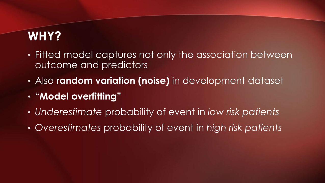
• Fitted model captures not only the association between outcome and predictors

• Also random variation (noise) in development dataset

• “Model overfitting”

• Underestimate probability of event in low risk patients

• Overestimates probability of event in high risk patients

WHY?

• Rule of thumb

• Events per variable (EPV) ratio

• EPV =Number of events

Number of regression coefficient

• EPV of ≥ 10 is needed to avoid overfitting

SAMPLE SIZE REQUIRED FOR RISK PREDICTION MODEL

• 60 events for model with 6 regression coefficients

EXAMPLE

CV Death

Age

Sex

Family History of

CVD

DM

HT

Structural Heart

Disease

• EPV of 10 may be difficult to achieve

WHEN EVENTS ARE RARE

• Models with few events compared to numbers of predictors often underperform when applied to new patients

• “Model Overfitting”

• Underestimate probability of event in low risk patients

• Overestimate probability of event in high risk patients

PROBLEM OF RARE OUTCOME

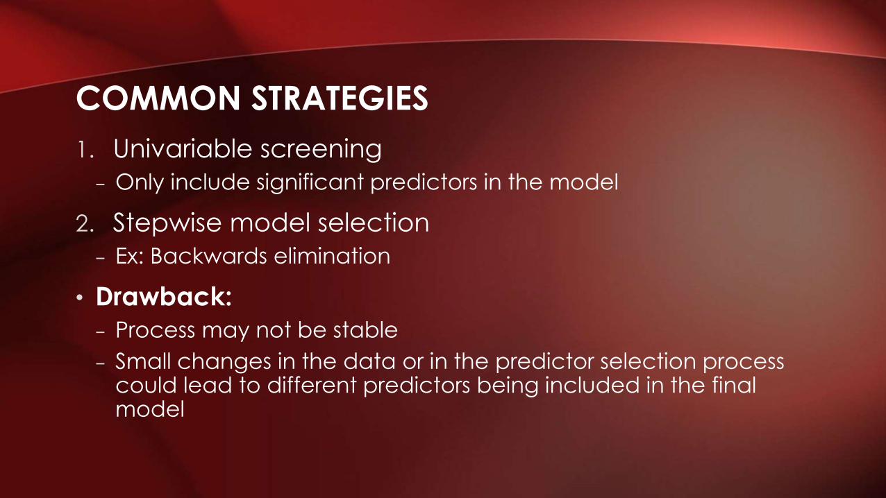
1. Univariable screening

– Only include significant predictors in the model

2. Stepwise model selection

– Ex: Backwards elimination

• Drawback:

– Process may not be stable

– Small changes in the data or in the predictor selection process could lead to different predictors being included in the final model

COMMON STRATEGIES

• “Shrinkage” methods

• Methods that tend to shrink the regression coefficient towards zero

• Moving poorly calibrated predicted risks towards the average risk

ANOTHER WAY TO ALLEVIATE MODEL FITTING

• Shrink all coefficients by common factor: ex. -20%

• However, this approach does not perform well if EPV very low

SIMPLEST SHRINKAGE METHOD

• Flexible shrinkage approaches that is effective when EPV is low (<10)

• Process:

1. Specify form of risk model (ex: logistic/Cox)

2. Fit the data to estimate coefficient in standard logistic/Cox model

3. Range of predicted risk is too wide as result of overfitting

4. Shrinking regression coefficients toward zero by placing constraint on the values of regression coefficients (Penalized)

• Coefficient estimates are typically smaller than those of standard regression

PENALIZED REGRESSION

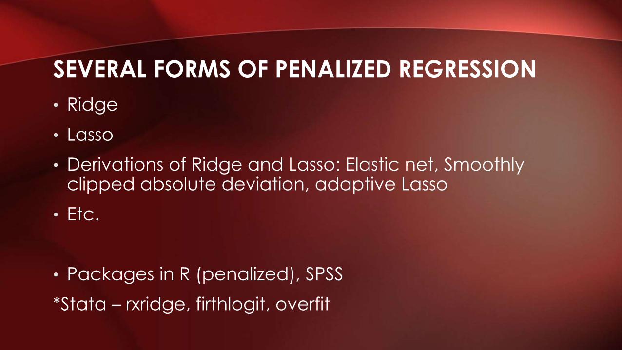
• Ridge

• Lasso

• Derivations of Ridge and Lasso: Elastic net, Smoothly clipped absolute deviation, adaptive Lasso

• Etc.

• Packages in R (penalized), SPSS

*Stata – rxridge, firthlogit, overfit

SEVERAL FORMS OF PENALIZED REGRESSION

• Fit model under constraint that sum of squared regression coefficients does not exceed particular threshold

• Penalized the coefficients using formula:

𝑙 𝛽 − 𝜆

𝑗=1

𝑝

𝛽𝑗2

• 𝜆 : scalar chosen by the investigator to control the amount of shrinkage– 𝜆 = 0 results in the standard regression model

RIDGE REGRESSION

• The threshold is chosen to maximize model’s predictive ability using cross validation:

– Dataset is split into k group

– Model is fitted to (k-1) groups and validated on the omitted group

– Repeated k times, each time omitting a different group

– Ex: 10-fold cross validation

• Split dataset into 10 subsets

• Subset j is omitted then penalized model is fitted to other nine subsets

• Calculate prediction for all patients, calculate predictive abilities and compare with the full model

• Least Absolute Shrinkage and Selection Operator

• Similar to ridge

• Constrain the sum of absolute values of regression coefficients

𝑙 𝛽 − 𝜆

𝑗=1

𝑝

𝛽𝑗

• Lasso can effectively exclude predictors from the final model by shrinking coefficient to 0

LASSO REGRESSION

• In health research, set of pre-specified predictors is often available

• Ridge regression is usually preferred option

• Lasso: if preferred simpler model with few predictors (ex: save time/resources by collecting less information on patients)

RIDGE OR LASSO?

• Assessment of model calibration

– Internal validation

– External validation

• Dividing patients into risk groups according to predicted risk

• Compare proportion of patients who had event and average predicted risk in that group

– Graph (calibration plot)

– Table (and Hosmer-Lemeshow GoF)

DETECTION OF MODEL OVERFITTING

• Quantify by simple regression model

• Outcomes in validation data are regressed using logistic regression on their predicted risk score

• Well-calibrated model: estimated slop (calibration slope): close to 1

• Overfitted model: <1 (low risks are underestimated, high risks are overestimated

DEGREE OF OVERFITTING

• Data of 3118 patients with mechanical heart valve

• Outcome: Failure of artificial valve (56)

• Predictor: age, sex, BSA, fractures in the batch of the valve (Y/N), year of valve manufacture (<1981/>1981), valve size (10 coefficients)

• EPV = 56/10 = 5.6

• Standard, ridge, lasso regression

EXAMPLE 1: MECHANICAL HEART VALVE FAILURE

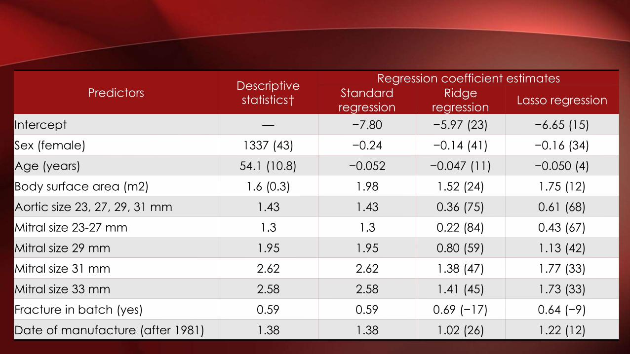
PredictorsDescriptive

statistics†

Regression coefficient estimates

Standard

regression

Ridge

regressionLasso regression

Intercept — −7.80 −5.97 (23) −6.65 (15)

Sex (female) 1337 (43) −0.24 −0.14 (41) −0.16 (34)

Age (years) 54.1 (10.8) −0.052 −0.047 (11) −0.050 (4)

Body surface area (m2) 1.6 (0.3) 1.98 1.52 (24) 1.75 (12)

Aortic size 23, 27, 29, 31 mm 1.43 1.43 0.36 (75) 0.61 (68)

Mitral size 23-27 mm 1.3 1.3 0.22 (84) 0.43 (67)

Mitral size 29 mm 1.95 1.95 0.80 (59) 1.13 (42)

Mitral size 31 mm 2.62 2.62 1.38 (47) 1.77 (33)

Mitral size 33 mm 2.58 2.58 1.41 (45) 1.73 (33)

Fracture in batch (yes) 0.59 0.59 0.69 (−17) 0.64 (−9)

Date of manufacture (after 1981) 1.38 1.38 1.02 (26) 1.22 (12)

FIG 1: DISTRIBUTION OF PREDICTED RISK SCORES ESTIMATED USING STANDARD, RIDGE, AND LASSO REGRESSION

Menelaos Pavlou et al. BMJ 2015;351:bmj.h3868

FIG 2: OBSERVED PROPORTIONS VERSUS AVERAGE PREDICTED RISK OF THE EVENT (USING STANDARD, RIDGE AND LASSO REGRESSION).

• Data on 1000 patients

• Outcome: risk of sudden cardiac death within 10 years from diagnosis (42 events)

• Predictors: age, max LV wall thickness, fractional shortening, LA diameter, peak LV outflow tract gradient (cont) andgender, family history of SCD, non-sustained VT, severity of HF by NYHA, unexplained syncope (binary)

• EPV = 4.2

• Externally validated model using data from different centers (2405 patients, 106 events)

EXAMPLE 2: SUDDEN CARDIAC DEATH IN HYPERTROPHIC CARDIOMYOPATHY

COEFFICIENT TABLE

Predictors

Regression coefficient estimates

Standard

regression

Ridge

regressionLasso regression

Age (years) -0.024 -0.015 -0.015

Max Wall Thickness (mm) 0.043 0.038 0.039

Fractional Shortening(mm) 0.002 0.003 0

LA diameter (mm) 0.042 0.028 0.027

Peak LVOT gradient (mmHg) 0.009 0.007 0.007

Sudden cardiac death in family 0.60 0.43 0.42

Non-sustain VT 0.30 0.19 0.03

Syncope 0.93 0.71 0.74

Sex-male -0.14 -0.07 0

NYHA class III/IV -0.24 -0.07 0

FIGURE

• When number of events is low compared to predictors in risk model: standard regression may produced overfitted risk model

• Common method such as stepwise selection and univariablescreening are problematic and should be avoided

• Recommended that the use of penalized regression methods be explored

• Other methods such as incorporated existing evidence (from published risk models, meta-analysis, and expert opinion) could be better in some scenario

CONCLUSION

• Beware prediction models with

EPV(Number of events

Number of regression coefficient) < 10

• Standard model usually “overfitted” in EPV<10: underestimate low risk patients, and overestimate high risk patients

• Penalizing the coefficient using penalized regression methods such as Ridge and Lasso is a possible solution to this problem

TAKE HOME MESSAGE

THANK YOU

http://www.ceb-rama.org

NEXT JOURNAL CLUB REMINDER:

Factors influencing recruitment to

research: qualitative study of the

experiences and perceptions of

research teams

by Threechada Boonchan

Friday 19th, February 13:00-14:30

Room 905 lunch from 12:00 noon Register at: www.ceb-rama.org

Tip: Use “Scan” app to scan QR code and add appointment