Risky Banks and Macroprudential Policy for EmergingEconomiesPreliminary Draft - December 1, 2014Please do not circulate

Gabriel Cuadra∗

Banco de Mexico

Victoria Nuguer†‡

Banco de Mexico

Abstract

We develop a two-country DSGE model with global banks (financial intermediaries in one countrylend to banks in the other country) in order to understand the consequences of cross-border bankingflows from the United States to emerging market economies (EME). Moreover, we look at the roleof EME’ macroprudential policy on mitigating the financial instability that the volatility of cross-border banking flows might cause. Banks in both countries are financially constrained on how muchthey can borrow from households. EME’ banks might also be constrained on how much they canborrow from U.S. banks because EME’ banks can be risky. A negative shock to the value of thecapital in the United States generates a global financial crisis through the cross-border bankingflows with outflows for the EME. Unconventional credit policy helps to mitigate the effects of afinancial disruption and causes inflows for the EME. Macroprudential policy targeting non-coreliabilities carried out by the EME helps to resilience the domestic economy to cross-border capitalflows and makes EME households better off.

JEL Classification: G28, E44, F40, G21.Keywords: Global banking; emerging market economies; financial frictions; macro-prudentialpolicy.

∗Address: Banco de Mexico, Direccion General de Investigacion Economica, Calle 5 de Mayo #18, 06059Ciudad de Mexico, Mexico; e-mail:gcuadra@banxico.org.mx.†Address: Banco de Mexico, Direccion General de Investigacion Economica, Calle 5 de Mayo #18, 06059

Ciudad de Mexico, Mexico; e-mail: vnuguer@banxico.org.mx.‡Any views expressed herein are those of the authors and do not necessarily reflect those of Banco de

Mexico. We are grateful to Julio Carrillo for his advice and guidance. We also thank Ana Marıa Aguilarand Jessica Roldan for their time to discuss and their helpful comments. All remaining errors are our own.

1

1 Introduction

Financial liberalization and progress in communication and information technologies havetriggered a significant increase in the degree of interconnectedness among financial insti-tutions, investors, and markets at an international level. In principle, these developmentshave allowed a more efficient allocation of resources and risk across countries and eco-nomic agents. However, this increased interdependence process has also led to a fastertransmission of financial shocks across economies. In particular, it has increased the ex-posure of emerging market economies (EMEs) to financial shocks originated in advancedeconomies. For example, the financial crisis of 2007-2009 originated in the U.S. housingsector and spread to a number of economies that had investments in the United Statesand also to those that received investment from the United States, such as EMEs. In theaftermath of the global financial crisis, the role of macro-prudential policies as measuresto preserve financial stability has been widely discussed among scholars and policy makersin recent years. In this context, we build a two-country model (advanced and emergingeconomies) to study the role of global financial intermediaries (banks that interact withother banks across international borders) in explaining the international transmission offinancial shocks from advanced economies to EMEs. Furthermore, we look at the effectsof U.S. unconventional policy for EMEs and how macro-prudential policies help to reducefinancial instability in EMEs.

The international financial crisis showed the role that global banks can play in spread-ing financial shocks across economies. In 2007, the problems in the U.S. housing sectorhit financial institutions and many banks found themselves in distress. This, in additionto the failure of Lehman Brothers in September 2008, triggered a severe liquidity crisis inthe interbank market. The spread between the interest rate on interbank loans and theU.S. T-bills increased 350bps. Assets in the United States started to lose value. U.S. banksdecreased their loans, including their foreign claims on EMEs counterparties. EMEs bankssaw an outflow of capital from global banks; their liability side was shrinking. Therefore,EMEs’ banks decided to decrease loans domestically, and the crisis transmitted from theUnited States to EMEs. As a results of the loss of the value of U.S. assets and the fall incredit in the United States, U.S. banks started to lend less to EMEs. At the end of 2008,the total foreign claims of U.S. banks with developing economies counterparties had fallenby almost 19% of the end of 2007’s level, almost $100 billion U.S. dollar.

It is important to remark that the crisis to EMEs was not only transmitted by globalbanks. The trade effect was the most important channel of transmission of the financialcrisis for these countries, especially because the EMEs’ banks did not hold U.S. mortgagebacked securities and in general the financial deepness is low in comparison with advancedeconomies. Furthermore, the magnitude of the effects prompted by the financial crisis wasdifferent across EMEs because of country specific characteristics. In this paper, we lookat Mexico, an EME that started to improve financial regulation and supervision after the1995 crisis, and Turkey, a stylized EME that hadn’t implemented macro-prudential until

2

the discussion of the Basel Agreements.As a result of the financial crisis, the Federal Reserve and other central banks intro-

duced a set of so-called “unconventional” monetary policies. In particular, the Fed startedto intervene directly in the credit market, lending to non-financial institutions and reducingthe restrictions to access to the discount window, among other policies. This helped torecover confidence in financial markets and capital started to move back to EMEs.

In this setting, loose monetary conditions in major advanced economies, such as theUnited States, contributed to an episode of large capital flows to EMEs. The magnitudeand speed at which these financial flows move raised some financial stability concerns inthe recipient economies, Sanchez (2013) and Powell (2013). Overall, capital flows can beallocated to different markets and assets, with different implications for the developmentof financial imbalances. For example, capital flows may be directly allocated to public orcorporate debt markets and/or intermediated through the domestic banking system. Inthe case of EMEs, several empirical studies find that episodes of large capital inflows in-crease the probability of credit booms. There are different channels through which capitalinflows may contribute to a credit expansion. There is a direct link between these inflowsand credit boom in those cases when financial inflows take the form of bank loans andare intermediated through domestic banks. Hence, some countries experienced growingfinancial imbalances.

On June 2013, the Federal Reserve announced that they would start the tapering ofsome of the unconventional policies (in particular quantitative easing) contingent on posi-tive economic data. This news prompted a decrease in U.S. stock markets. Capital startedto flight back to advances economies, creating financial instability in EMEs. In this con-text, an important concern is the risk of reversals in financial flows, with a negative impacton the banking credit granted to the private sector in EMEs. This risk is latent due to theuncertainty about the normalization of monetary conditions in the United States. Thissituation has already contributed to some periods of high volatility in international finan-cial markets, which affected EMEs. Therefore, these economies are vulnerable to externalshocks. In particular, shocks in the United States or the Federal Reserve’s policy decisionsmight prompt capital to move around the globe. The main concerns are debt (portfo-lio) flows and cross-border bank lending because they might cause financial instability inEMEs, BIS (2010b).

In light of the exposure of these economies to financial shocks originated in advancedeconomies, authorities must design and implement policy actions aimed at reducing fi-nancial stability risks. In this setting, a key issue concerns the role of macro-prudentialpolicies in addressing these risks. Macro-prudential policies are thought to limit the riskof widespread disruptions to the provision of financial services that have negative conse-quences for the economy. It focuses on the interactions between the financial and the realsector, and not just individual banks. Macro-prudential instruments are mainly prudentialtools that target the sources of systemic risk (FSB, IMF, and BIS, 2011). In principle,these instruments strengthen the resilience of the financial markets and institutions they

3

050

100

150

Bill

ion

US

Dol

lars

01

23

4T

rillio

n U

S D

olla

rs

2001q4 2003q4 2005q4 2007q4 2009q4 2011q4 2013q4

Offshore centres

Developing countries

Developed countries

Mexico (right axis)

Brasil (right axis)

Turkey (right axis)

Russia (right axis)

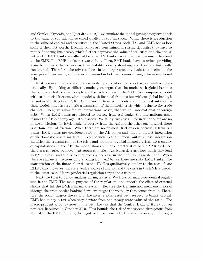
Source: BIS Consolidated Bank Statistics, Inmediate Borrower Basis.

Foreign claims of US reporting banks on individual countries

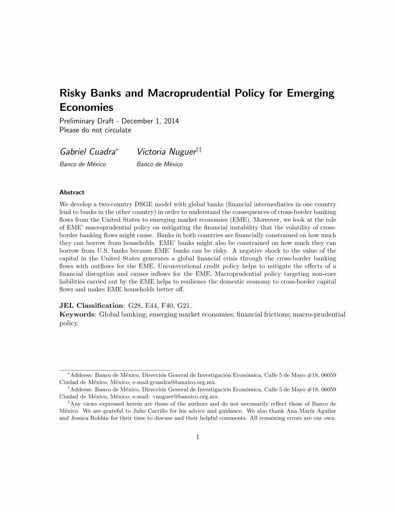
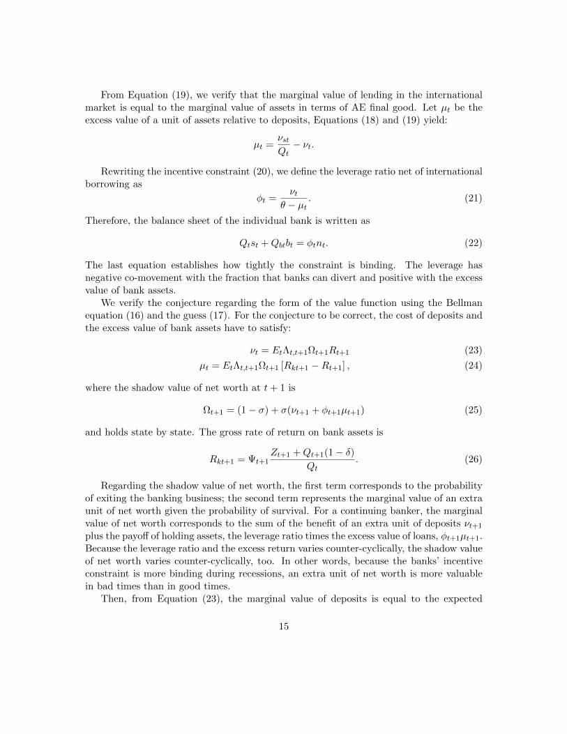
Fig. 1. Foreign Claims of U.S. Reporting Banks on Individual Countries, 1999Q4-2014Q1

target. Although there is no conclusive evidence, the empirical literature supports theeffectiveness of macro-prudential tools in dampening procyclicality in financial markets,particularly when those tools target banks. Under this framework macro-prudential poli-cies in EMEs can help to control the financial volatility (and therefore, the real economyvolatility) that foreign exposure might cause. That is, EMEs have tools to limit the effectsof external shocks on the financial system. Summing up, the financial crisis and the periodsof financial turmoil in mid-2013 and early 2014, reminded us that financial instability inEMEs is a risk that policy makers should be aware of and macro-prudential policy is onetool on helping to reduce it.

Figure 1 documents the foreign claims of U.S. banks by EMEs from 2001Q4 until2014Q1. Developing economies correspond to 26% of the total of foreign claims as an av-erage of the sample. Mexico is the non-advanced economy that receives the most foreignclaims from U.S. reporting banks, in terms of Mexican GDP they are on average almost9% points and they are 5% of the total foreign claims of U.S. banks. The sum of foreignU.S. claims on Brazil, Mexico, Turkey, and Russia is on average 5% of the total GDP ofthose countries. Foreign claims shows a positive trend for the sample. There is a clearfall in September 2008, when Lehman Brothers failed and a sharp recovery afterwards, asa consequence of unconventional monetary policy. For the last year of data there is nota clear tendency of where the claims of U.S. banks are going, but Mexico, Brazil, Russia,and Turkey show some level of slowdown.

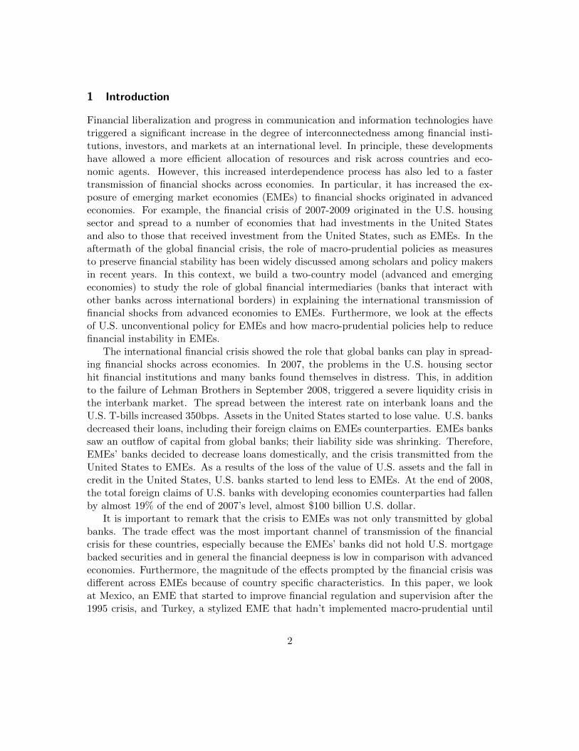
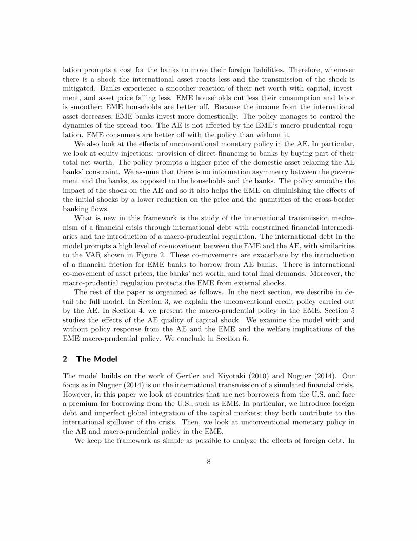
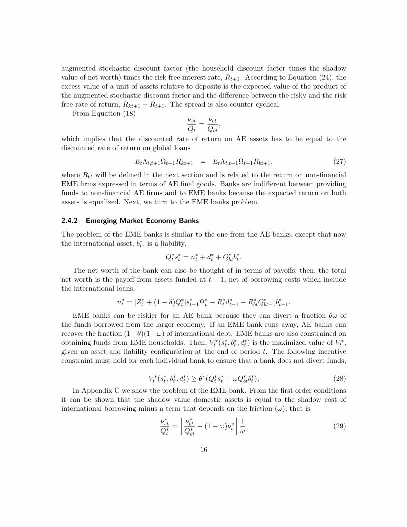
To understand better the transmission through banks of the financial crisis from theUnited States to EMEs, we estimate a VAR. Figure 2 shows the orthogonalized impulse

4

responses functions from a VAR with one lag with U.S. and two EMEs data: Mexico (solidgray line) and Turkey (dashed blue line). The core VAR consists of six variables: real netcharge-offs on all loans and leases of U.S. banks, the S&P500 index, real foreign U.S. banks’claims with EME counterparties, real EME GDP, real EME banks’ credit to the privatenon-financial sector, exchange rate of EME domestic currency per U.S. dollar, and theEME stock market index. For Mexico, the data goes from 2002Q1 to 2013Q4. And forTurkey the data goes from 2001Q3 to 2013Q3.1 All data are in log and detrended usingthe Hodrick-Prescott filter. The starting point corresponds to the availability of the EMEsdata. The Cholesky ordering corresponds to the order of the listed variables.2

The VAR exposes the response to a one-standard deviation innovation to the netcharge-offs on all loans and leases in bank credit for all U.S. commercial banks. The shockcaptures one of the initial characteristics of the financial crisis: the decrease in the value ofthe U.S. banks’ loans. The shock suggests a decrease in the S&P 500 index and a decreasein the loans that U.S. banks make to the EME. Then, the crisis is transmitted to the EME,where the GDP, the total loans to the private non-financial sector and the stock marketindex fall. The exchange rate between EME domestic currency and U.S. dollar increasesuggesting a deterioration of the domestic currency because of the loans flying away fromthe country. The VAR highlights a significant and negative reaction of the EME (real andfinancial) economy to a decrease in the U.S. banks’ net charge-off on all loans and leases.Furthermore, the co-movement of the stock indexes suggests a strong cross-country relationof the asset prices. While U.S. loans go down because of the shock, the decrease on theloans of U.S. banks to the EME emphasizes the co-movement across countries promptingfinancial instability in the EME. The two EME show similar response to the initial shock.However, the estimated VAR results on a larger impact on the Turkish economy. Thishighlights how the Turkish economy, one without macro-prudential regulation is hit harderby a foreign shock than the Mexican economy, an economy that started to improve financialregulation and supervision in the mid-90s. In this paper, we build a dynamic stochasticgeneral equilibrium model (henceforth DSGE) that explains these interactions.

We propose a two-country (advance and emerging economies) model with global banksand financial frictions to examine the international transmission of a financial crisis throughthe international debt market. The EME is a relatively small country with a small bankingsector, such as Mexico or Turkey, while the advance economy (AE) is a big economy witha big banking sector, such as the United States. The model builds on the closed economy

1 See Appendix for the definition and the sources of the data. we use Mexican banks’ credit to the privatenon-financial sector and not the new loans of Mexican banks because the former starts before. Moreoverthis data is comparable to the one for Turkish banks.

2 The Akaike information criterion (AIC) suggests the use of one lag. Given the comments of Kilian(2011), we performed different robustness checks. Changing the order for the Cholesky decomposition ofthe Mexican variables does not alter the behavior of the IRF. Including the difference between the Mexicaninterest rate on new loans and the interest rate on deposit before the Mexican stock market index promptsa similar reaction of the VAR with the spread increasing after a positive shock to the net charge-offs ofU.S. banks.

5

-.05

0.0

5.1

.15

.2

0 5 10 15

U.S. NCO

-.04

-.03

-.02

-.01

0.0

1

0 5 10 15

S&P 500

-.03

-.02

-.01

0

0 5 10 15

Foreign claims of U.S. banks

-.01

5-.

01-.

005

0

0 5 10 15

EME GDP

-.03

-.02

-.01

0

0 5 10 15

Dom. Bank Credit

-.01

0.0

1.0

2

0 5 10 15

EME Exchange Rate

-.06

-.04

-.02

0.0

2

0 5 10 15

Turkey Mexico

EME Stock Mkt Index

Impulse Responses to Cholesky One-Std-Dev. Innovation to NCO on Commercial US Banks.

Fig. 2. VAR EvidenceNote: Mexican VAR estimated for 2002Q1 to 2013Q4. The Cholesky ordering is U.S. net charge-offs,

S&P500, U.S. banks’ foreign claims on Mexican banks, Mexican GDP, Mexican banks credit to the private

non-financial sector, exchange rate of Mexican pesos per U.S. dollar and the Mexican stock market index.

Turkish VAR estimated for 2001Q3 to 2013Q3. The Cholesky ordering of the variables is similar to the

Mexican case. The vertical axis shows the percent deviation from the baseline.a

a Country VAR estimated with 1 standard deviations confident intervals are available by request. Theresults are robust to this specification.

models of Gertler and Kiyotaki (2010) and Gertler and Karadi (2011) and the open econ-omy set up of Nuguer (2014). There are advance and emerging banks. They use their networth and local deposits to finance domestic non-financial business. Although banks canfinance local businesses by buying their securities without friction, they face a financingconstraint in raising deposit from local households because banks are subject to a moralhazard problem. AE banks (U.S. banks) have a longer average lifetime and a larger networth (relative to the size of the economy) than EME banks; as a consequence, AE bankslend to EME banks using international debt and effectively participate in risky finance inthe EME market.

As in the previous literature (Gertler and Kiyotaki (2010), Gertler and Karadi (2011),

6

and Gertler, Kiyotaki, and Queralto (2012)), we simulate the model giving a negative shockto the value of capital, the so-called quality of capital shock. When there is a reductionin the value of capital and securities in the United States, both U.S. and EME banks losesome of their net worth. Because banks are constrained in raising deposits, they have toreduce financing businesses, which further depresses the value of securities and the banks’net worth. EME banks are affected because U.S. banks have to reduce how much they lendto the EME. The EME banks’ net worth falls. Then, EME banks have to reduce providingloans to domestic firms because their liability side is shrinking and they are financiallyconstrained. Therefore, the adverse shock in the larger economy leads to a decline in theasset price, investment, and domestic demand in both economies through the internationaldebt.

First, we examine how a country-specific quality of capital shock is transmitted inter-nationally. By looking at different models, we argue that the model with global banks isthe only one that is able to replicate the facts shown in the VAR. We compare a modelwithout financial frictions with a model with financial frictions but without global banks, ala Gertler and Kiyotaki (2010). Countries in these two models are in financial autarky. Inthese models there is very little transmission of the financial crisis which is due to the tradechannel. Then, we allow for an international asset, that we call international or foreigndebt. When EME banks are allowed to borrow from AE banks, the international assetinsures the AE economy against the shock. We study two cases. One in which there are nofinancial frictions for EME banks to borrow from the AE and the other one in which thereis certain level of friction. When there are no financial frictions on borrowing from AEbanks, EME banks are considered safe by the AE banks and there is perfect integrationof the domestic assets markets. In comparison to the financial autarky case, integrationamplifies the transmission of the crisis and prompts a global financial crisis. To a qualityof capital shock in the AE, the model shows similar characteristics to the VAR evidence:there is asset price co-movement across countries, AE banks decrease how much they lendto EME banks, and the AE experiences a decrease in the final domestic demand. Whenthere are financial frictions on borrowing from AE banks, there are risky EME banks. Thetransmission of the financial crisis to the EME is qualitatively similar to the case of safeEME banks, however there is an extra source of friction and the crisis in the EME is deeperin the latest case. Macro-prudential regulation targets this friction.

Next, we turn to policy analysis during a crisis. We focus on macro-prudential regula-tion in the EME. The main purpose of the regulation is to smooth the effect of externalshocks that hit the EME’s financial system. Because the transmission mechanism worksthrough the cross-border banking flows, we target the volatility that comes from it. There-fore, the policy targets the ratio of the international asset with respect to banks’ capital.EME banks pay a tax when they deviate from the steady state value of the ratio. Themacro-prudential policy goes in line with the tax that the Central Bank of Korea put onnon-core liabilities in October 2010. This bounds the risk of widespread disruptions fromabroad to the EME, limiting the negative consequences for the small economy. This regu-

7

lation prompts a cost for the banks to move their foreign liabilities. Therefore, wheneverthere is a shock the international asset reacts less and the transmission of the shock ismitigated. Banks experience a smoother reaction of their net worth with capital, invest-ment, and asset price falling less. EME households cut less their consumption and laboris smoother; EME households are better off. Because the income from the internationalasset decreases, EME banks invest more domestically. The policy manages to control thedynamics of the spread too. The AE is not affected by the EME’s macro-prudential regu-lation. EME consumers are better off with the policy than without it.

We also look at the effects of unconventional monetary policy in the AE. In particular,we look at equity injections: provision of direct financing to banks by buying part of theirtotal net worth. The policy prompts a higher price of the domestic asset relaxing the AEbanks’ constraint. We assume that there is no information asymmetry between the govern-ment and the banks, as opposed to the households and the banks. The policy smooths theimpact of the shock on the AE and so it also helps the EME on diminishing the effects ofthe initial shocks by a lower reduction on the price and the quantities of the cross-borderbanking flows.

What is new in this framework is the study of the international transmission mecha-nism of a financial crisis through international debt with constrained financial intermedi-aries and the introduction of a macro-prudential regulation. The international debt in themodel prompts a high level of co-movement between the EME and the AE, with similaritiesto the VAR shown in Figure 2. These co-movements are exacerbate by the introductionof a financial friction for EME banks to borrow from AE banks. There is internationalco-movement of asset prices, the banks’ net worth, and total final demands. Moreover, themacro-prudential regulation protects the EME from external shocks.

The rest of the paper is organized as follows. In the next section, we describe in de-tail the full model. In Section 3, we explain the unconventional credit policy carried outby the AE. In Section 4, we present the macro-prudential policy in the EME. Section 5studies the effects of the AE quality of capital shock. We examine the model with andwithout policy response from the AE and the EME and the welfare implications of theEME macro-prudential policy. We conclude in Section 6.

2 The Model

The model builds on the work of Gertler and Kiyotaki (2010) and Nuguer (2014). Ourfocus as in Nuguer (2014) is on the international transmission of a simulated financial crisis.However, in this paper we look at countries that are net borrowers from the U.S. and facea premium for borrowing from the U.S., such as EME. In particular, we introduce foreigndebt and imperfect global integration of the capital markets; they both contribute to theinternational spillover of the crisis. Then, we look at unconventional monetary policy inthe AE and macro-prudential policy in the EME.

We keep the framework as simple as possible to analyze the effects of foreign debt. In

8

line with the previous literature, we focus on a real economy, abstracting from nominalfrictions. First, we present the physical setup, a two country real business cycle model withtrade in goods. Second, we add financial frictions. We introduce banks that intermediatefunds between households and non-financial firms. Financial frictions constrain the flowof funds from households to banks. A new feature of this model is that AE banks caninvest in the EME by lending to EME banks. Moreover, we assume that EME banksare constrained on how much they can borrow from AE banks. EME banks also face apremium on the interest rate payed to AE banks. Households and non-financial firms arestandard and described briefly, while we explain in more detail the financial firms. In whatfollows, we describe the AE; otherwise specified, the EME is symmetric. EME variablesare expressed with an ∗.

2.1 Physical Setup

There are two countries in the world: advance economy (AE) and emerging economy(EME). Each country has a continuum of infinitely lived households. In the global economy,there is also a continuum of firms of mass unity. A fraction m corresponds to the AE, whilea fraction 1−m to the EME. Using an identical Cobb-Douglas production function, eachof the firms produces output with domestic capital and labor. Aggregate AE capital, Kt,and aggregate AE labor hours, Lt, are combined to produce an intermediate good Xt inthe following way:

Xt = AtKαt L

1−αt , with 0 < α < 1, (1)

where At is the productivity shock.With Kt as the capital stock at the end of period t and St as the aggregate capital

stock “in process” for period t+ 1, we define

St = It + (1− δ)Kt (2)

as the sum of investment, It, and the undepreciated capital, (1− δ)Kt. Capital in process,St, is transformed into final capital, Kt+1, after taking into account the quality of capitalshock, Ψt+1,

Kt+1 = StΨt+1. (3)

Following the previous literature, the quality of capital shock introduces an exogenousvariation in the value of capital. The shock affects asset price dynamics, because the latteris endogenous. The disruption refers to economic obsolesce, in contrast with physicaldepreciation. The shocks Ψt and Ψ∗t are mutually independent and i.i.d. The AE qualityof capital shock serves as a trigger for the financial crisis.

As in Heathcote and Perri (2002), there are local perfectly competitive distributor firmsthat combine domestic and imported goods to produce final goods. These are used for

9

consumption and investment, and are produced using a constant elasticity of substitutiontechnology

Yt =

[ν

1ηX

H η−1η

t + (1− ν)1ηX

F η−1η

t

] ηη−1

, (4)

where η is the elasticity of substitution between domestic and imported goods. There ishome bias in production. The parameter ν is a function of the size of the economy and thedegree of openness, λ: ν = 1− (1−m)λ (Sutherland, 2005).

Non-financial firms acquire new capital from capital good producers, who operate ata national level. As in Christiano, Eichenbaum, and Evans (2005), there are convex ad-justment costs in the gross rate of investment for capital goods producers. Then, the finaldomestic output equals domestic households’ consumption, Ct, domestic investment, It,and government consumption, Gt,

Yt = Ct + It

[1 + f

( ItIt−1

)]+Gt. (5)

Turning to preferences, households maximize their expected discounted utility

U(Ct, Lt) = Et

∞∑t=0

βt[

lnCt −χ

1 + γL1+γt

], (6)

where Et is the expectation operator conditional on information available on date t, andγ is the inverse of Frisch elasticity. We abstract from many features in the conventionalDSGE models, such as habit in consumption, nominal prices, wage rigidity, etc.

In Appendix B, we define the competitive equilibrium of the frictionless economy whichis the benchmark when comparing the different models with financial frictions. It is astandard international real business cycle model in financial autarky with trade in goods.Next, we add financial frictions.

2.2 Households

There is a representative household for each country. The household is composed of acontinuum of members. A fraction f are bankers, while the rest are workers. Workerssupply labor to non-financial firms, and return their wages to the households. Each ofthe bankers manages a financial intermediary and transfers non negative profits back toits household subject to its flow of funds constraint. Within the family, there is perfectconsumption insurance.

Households deposit funds in a bank; we assume that they cannot hold capital directly.Deposits are riskless one period securities, and they pay Rt return, determined in periodt− 1.

Households choose consumption, deposits, and labor (Ct, Dht , and Lt, respectively)

10

by maximizing expected discounted utility, Equation (6), subject to the flow of fundsconstraint,

Ct +Dht+1 = WtLt +RtD

ht + Πt − Tt, (7)

where Wt is the wage rate, Πt are the profits from ownership of banks and non-financialfirms, and Tt are lump sum taxes. The first order conditions for the problem of thehouseholds are

Lt : WtCt

= χLγt (8)

Dht+1 : EtRt+1β

CtCt+1

= EtRt+1Λt,t+1 = 1 (9)

with Λt,t+1 as the stochastic discount factor.

2.3 Non-financial firms

2.3.1 Goods producers

Intermediate competitive goods producers operate at a local level with constant returns toscale technology with capital and labor as inputs, given by Equation (1). Wage is definedby

Wt = (1− α)PHt Kαt Lt

−α with PHt = ν1η Y −1

t

(XHt

)− 1η . (10)

The price of the final AE good is equalized to 1. The gross profits per unit of capital Ztare

Zt = αPHt L1−αt Kt

α−1. (11)

To simplify, we assume that non-financial firms do not face any financial frictions whenobtaining funds from intermediaries and they can commit to pay all future gross profitsto the creditor bank. A good producer will issue new securities at price Qt to obtainfunds for buying new capital. Because there is no financial friction, each unit of securityis a state-contingent claim to the future returns from one unit of investment. By perfectcompetition, the price of new capital equals the price of the security and goods producersearn zero profits state-by-state.

The production of these competitive goods is used locally and abroad,

Xt = XHt +

1−mm

XH∗t (12)

to produce the final good Yt following the CES technology shown in Equation (4). Then,the demands faced by the intermediate competitive goods producers are

XHt = ν

[PHtPt

]−ηYt (13)

11

and

XH∗t = ν∗

[PH∗t

P ∗t

]−ηY ∗t ,

where Pt is the price of the AE final good, PHt the domestic price of AE goods, and PH∗t

the price of the AE good abroad. By the law of one price, PH∗t NERt = PHt with NERt asthe nominal exchange rate. Rewriting the price of the final good yields

Pt =[ν(PHt )1−η + (1− ν)(PFt )1−η] 1

1−η

Pt

PHt= [ν + (1− ν)τ1−η

t ]1

1−η ,

where τt is the terms of trade, the price of imports, relative to exports. Because of homebias in the final good production, Pt 6= P ∗t NERt; the real exchange rate is defined by

εt =P ∗t NERt

Pt. An increase in τt implies a deterioration (appreciation) of the terms of trade

for the AE (EME).

2.3.2 Capital producers

Capital producers use final output, Yt, to make new capital subject to adjustment costs.They sell new capital to goods producers at price Qt. The objective of non-financial firmsis to maximize their expected discounted profits, choosing It

maxIt

Et

∞∑τ=t

Λt,τ

QτIτ −

[1 + f

(IτIτ−1

)]Iτ

.

The first order condition yields the price of capital goods, which equals the marginal costof investment

Qt = 1 + f

(ItIt−1

)+

ItIt−1

f ′(

ItIt−1

)− EtΛt,t+1

[It+1

It

]2

f ′(It+1

It

). (14)

Profits, which arise only out of the steady state, are redistributed lump sum to households.

2.4 Banks

To finance their lending, banks get funds from national households and use retained earn-ings from previous periods. Banks are constrained on how much they can borrow fromhouseholds. In order to limit the banker’s ability to save to overcome being financiallyconstrained, inside the household we allow for turnovers between bankers and workers. Weassume that with i.i.d. probability σ a banker continues being a banker next period, whilewith probability 1−σ it exits the banking business. If it exits, it transfers retained earningsback to its household, and becomes a worker. To keep the number of workers and bankers

12

fixed, each period a fraction of workers becomes bankers. A bank needs positive funds tooperate, therefore every new banker receives a start-up constant fraction ξ of total assetsof the bank.

To motivate cross-border banking flows, we assume that the survival rate of the AEbanks σ is higher that of the EME banks σ∗. Then, the AE banks can accumulate more networth to operate. In equilibrium, AE banks lend to EME banks. This interaction betweenAE and EME banks is what we call international or foreign debt/asset. AE banks fundtheir activity through a retail market (deposits from households) and EME banks fundtheir lending through a retail and an international wholesale market (where AE banks lendto EME banks).

At the beginning of each period, a bank raises funds from households, deposits dt, andretain earnings from previous periods which we call net worth nt; it decides how much tolend to non-financial firms st. AE banks also choose how much to lend to EME banks bt.

Banks are constrained on how much they can borrow from households. In this sense,financial frictions affect the real economy. By assumption, there is no friction when transfer-ring resources to non-financial firms. Firms offer banks a perfect state-contingent security,st. The price of the security (or loan) is Qt, which is also the price of the assets of thebank. In other words, Qt is the market price of the bank’s claim on the future returns fromone unit of present capital of non-financial firm at the end of period t, which is in processfor period t+ 1.

Next, we describe the characteristics of the AE and the EME banks.

2.4.1 Advance Economy Banks

For an individual AE bank, the balance sheet implies that the value of the loans funded inthat period, Qtst plus Qbtbt, where Qbt is the price of foreign debt, has to equal the sumof bank’s net worth nt and domestic deposits dt,

Qtst +Qbtbt = nt + dt.

Let Rbt be the cross-border banking flows rate of return from period t− 1 to period t.The net worth of an individual AE bank at period t is the payoff from assets funded att− 1, net borrowing costs:

nt = [Zt + (1− δ)Qt]st−1Ψt +Rb,tQbt−1bt−1 −Rtdt−1,

where Zt is the dividend payment at t on loans funded in the previous period, and is definedin Equation (11).

At the end of period t, the bank maximizes the present value of future dividends takinginto account the probability of continuing being a banker in the next periods; the value ofthe bank is defined by

Vt = Et

∞∑i=1

(1− σ)σi−1Λt,t+int+i.

13

Following the previous literature, we introduce a simple agency problem to motivatethe ability of the bank to obtain funds. After the bank obtains funds, it may transfer afraction θ of assets back to its own household. Households limit the funds lent to banks.

If a bank diverts assets, it defaults on its debt and shuts down. Its creditors can re-claim the remained 1− θ fraction of assets. Let Vt(st, bt, dt) be the maximized value of Vt,given an asset and liability configuration at the end of period t. The following incentiveconstraint must hold for each individual bank to ensure that the bank does not divertfunds:

Vt(st, bt, dt) ≥ θ(Qtst +Qbtbt). (15)

The borrowing constraint establishes that for households to be willing to supply funds to abank, the value of the bank must be at least as large as the benefits from diverting funds.

At the end of period t−1, the value of the bank satisfies the following Bellman equation

V (st−1, bt−1, dt−1) = Et−1Λt−1,t

(1− σ)nt + σ

[maxst,bt,dt

V (st, bt, dt)

]. (16)

The problem of the bank is to maximize Equation (16) subject to the borrowing constraint,Equation (15).

We guess and verify that the form of the value function of the Bellman equation islinear in assets and liabilities,

V (st, bt, dt) = νstst + νbtbt − νtdt, (17)

where νst is the marginal value of assets at the end of period t, νbt, the marginal value ofglobal lending, and νt, the marginal cost of deposits.

Maximizing the objective function (16) subject to (15), with λt as the constraint mul-tiplier, yields the following first order conditions:

st : νst − λt(νst − θQt) = 0

bt : νbt − λt(νbt − θQbt) = 0

dt : νt − λtνt = 0

λt : θ(Qtst +Qbtbt)− νstst + νbtbt − νtdt = 0.

Rearranging terms yields:

(νbt − νt)(1 + λt) = λtθQbt (18)(νstQt− νbtQbt

)(1 + λt) = 0 (19)[

θ −(νstQt− νt

)]Qtst +

[θ −

(νbtQbt− νt

)]Qbtbt = νtnt. (20)

14

From Equation (19), we verify that the marginal value of lending in the internationalmarket is equal to the marginal value of assets in terms of AE final good. Let µt be theexcess value of a unit of assets relative to deposits, Equations (18) and (19) yield:

µt =νstQt− νt.

Rewriting the incentive constraint (20), we define the leverage ratio net of internationalborrowing as

φt =νt

θ − µt. (21)

Therefore, the balance sheet of the individual bank is written as

Qtst +Qbtbt = φtnt. (22)

The last equation establishes how tightly the constraint is binding. The leverage hasnegative co-movement with the fraction that banks can divert and positive with the excessvalue of bank assets.

We verify the conjecture regarding the form of the value function using the Bellmanequation (16) and the guess (17). For the conjecture to be correct, the cost of deposits andthe excess value of bank assets have to satisfy:

νt = EtΛt,t+1Ωt+1Rt+1 (23)

µt = EtΛt,t+1Ωt+1 [Rkt+1 −Rt+1] , (24)

where the shadow value of net worth at t+ 1 is

Ωt+1 = (1− σ) + σ(νt+1 + φt+1µt+1) (25)

and holds state by state. The gross rate of return on bank assets is

Rkt+1 = Ψt+1Zt+1 +Qt+1(1− δ)

Qt. (26)

Regarding the shadow value of net worth, the first term corresponds to the probabilityof exiting the banking business; the second term represents the marginal value of an extraunit of net worth given the probability of survival. For a continuing banker, the marginalvalue of net worth corresponds to the sum of the benefit of an extra unit of deposits νt+1

plus the payoff of holding assets, the leverage ratio times the excess value of loans, φt+1µt+1.Because the leverage ratio and the excess return varies counter-cyclically, the shadow valueof net worth varies counter-cyclically, too. In other words, because the banks’ incentiveconstraint is more binding during recessions, an extra unit of net worth is more valuablein bad times than in good times.

Then, from Equation (23), the marginal value of deposits is equal to the expected

15

augmented stochastic discount factor (the household discount factor times the shadowvalue of net worth) times the risk free interest rate, Rt+1. According to Equation (24), theexcess value of a unit of assets relative to deposits is the expected value of the product ofthe augmented stochastic discount factor and the difference between the risky and the riskfree rate of return, Rkt+1 −Rt+1. The spread is also counter-cyclical.

From Equation (18)νstQt

=νbtQbt

,

which implies that the discounted rate of return on AE assets has to be equal to thediscounted rate of return on global loans

EtΛt,t+1Ωt+1Rkt+1 = EtΛt,t+1Ωt+1Rbt+1, (27)

where Rbt will be defined in the next section and is related to the return on non-financialEME firms expressed in terms of AE final goods. Banks are indifferent between providingfunds to non-financial AE firms and to EME banks because the expected return on bothassets is equalized. Next, we turn to the EME banks problem.

2.4.2 Emerging Market Economy Banks

The problem of the EME banks is similar to the one from the AE banks, except that nowthe international asset, b∗t , is a liability,

Q∗t s∗t = n∗t + d∗t +Q∗btb

∗t .

The net worth of the bank can also be thought of in terms of payoffs; then, the totalnet worth is the payoff from assets funded at t − 1, net of borrowing costs which includethe international loans,

n∗t = [Z∗t + (1− δ)Q∗t ]s∗t−1Ψ∗t −R∗t d∗t−1 −R∗btQ∗bt−1b∗t−1.

EME banks can be riskier for an AE bank because they can divert a fraction θω ofthe funds borrowed from the larger economy. If an EME bank runs away, AE banks canrecover the fraction (1−θ)(1−ω) of international debt. EME banks are also constrained onobtaining funds from EME households. Then, V ∗t (s∗t , b

∗t , d∗t ) is the maximized value of V ∗t ,

given an asset and liability configuration at the end of period t. The following incentiveconstraint must hold for each individual bank to ensure that a bank does not divert funds,

V ∗t (s∗t , b∗t , d∗t ) ≥ θ∗(Q∗t s∗t − ωQ∗btb∗t ), (28)

In Appendix C we show the problem of the EME bank. From the first order conditionsit can be shown that the shadow value domestic assets is equal to the shadow cost ofinternational borrowing minus a term that depends on the friction (ω); that is

ν∗stQ∗t

=

[ν∗btQ∗bt− (1− ω)ν∗t

]1

ω. (29)

16

If ω = 1, EME banks cannot run away with international debt and the second term inbrackets in the RHS is zero, therefore there is perfect asset market integration. In termsof returns:

EtΛ∗t,t+1Ω∗t+1R

∗kt+1 = EtΛ

∗t,t+1Ω∗t+1R

∗bt+1. (30)

On the other hand if 0 < ω < 1, the second term inside the brackets in the RHSof Equation (29) is positive. This means that the interest rate on foreign debt is lowerthan the rate of return on domestic capital, but higher than the deposit interest rate. In

Appendix C, we show that if µ∗t =ν∗stQ∗t− ν∗t and µ∗bt =

ν∗btQ∗bt− ν∗t ,

µ∗bt = ωµ∗t . (31)

Therefore, when ω = 1 (0 < ω < 1) the expected discounted rate of return on inter-national debt is equal to (less than) the expected discounted rate of return of loans tonon-financial EME firms. Given a shock, the return on the international debt is as volatileas the return on the domestic asset, emphasizing the transmission mechanism from onecountry to the other. Furthermore, when ω = 1 the expected discounted rate of returnon the global asset equalizes to the one on loans to non-financial AE firms, see Equation(27). Then, the AE loan market and the EME loan market behave in a similar way. Thisis the integration of the asset markets. When 0 < ω < 1, the rates equalized but there isan extra term, and that is why we call this case imperfect asset market integration; EMEbanks face an extra friction.

With Ω∗t+1 as the shadow value of net worth at date t+ 1, and R∗kt+1 as the gross rateof return on bank assets, after verifying the conjecture of the value function:

ν∗t = EtΛ∗t,t+1Ω∗t+1R

∗t+1, (32)

µ∗t = EtΛ∗t,t+1Ω∗t+1

[R∗kt+1 −R∗t+1

], and (33)

µ∗bt = EtΛ∗t,t+1Ω∗t+1

[R∗bt+1 −R∗t+1

](34)

with

Ω∗t+1 = 1− σ∗ + σ∗(ν∗t+1 + φ∗t+1µ

∗t+1

),

R∗kt+1 = Ψ∗t+1

Z∗t+1 +Q∗t+1(1− δ)Q∗t

, and (35)

R∗bt+1 =Z∗t+1 +Q∗bt+1(1− δ)

Q∗bt. (36)

2.4.3 Aggregate Bank Net Worth

Finally, aggregating across AE banks, from Equation (22):

QtSt +QbtBt = φtNt. (37)

17

Capital letters indicate aggregate variables. From the previous equation, we define thehouseholds deposits

Dt = Nt(φt − 1). (38)

Furthermore,

Nt = (σ + ξ) Rk,tQt−1St−1 +Rb,tQb,t−1Bt−1 − σRtDt−1. (39)

The last equation specifies the law of motion of the AE banking system’s net worth. Thefirst term in the curly brackets represents the return on loans made last period. The secondterm in the curly brackets is the return on funds that the household invested in the EME.Both loans are scaled by the old bankers (that survived from the last period) plus thestart-up fraction of loans that young bankers receive. The last term in the equation is thetotal return on households’ deposits that banks need to pay back.

For EME banks, the aggregation yields

N∗t = (σ∗ + ξ∗)R∗k,tQ∗t−1S

∗t−1 − σ∗R∗tD∗t−1 − σ∗R∗btQ∗bt−1B

∗t−1, (40)

where R∗bt equals R∗kt, from Equation (30). The balance sheet of the aggregate EME bankingsystem can be written as

Q∗tS∗t − ωQ∗btB∗t = φ∗tN

∗t . (41)

EME households deposits are given by

D∗t + (1− ω)Q∗btB∗t = N∗t (φ∗t − 1). (42)

2.4.4 Cross-border banking flows

At the steady state, AE banks invest in the EME because the survival rate of AE banks ishigher than the survival rate of EME banks; therefore, AE banks lend to EME banks. Aninternational asset market arises. EME banks have an incentive to borrow from AE banksbecause EME banks are more constrained than AE banks.

The small economy is an EME, therefore we assume that EME banks need to pay apremium on borrowing from AE banks. Following Schmitt-Grohe and Uribe (2003), theinterest rate payed by EME banks on the international debt is debt elastic. Specifically,Equation (27) becomes

EtΛt,t+1Ωt+1Rkt+1 = EtΛt,t+1Ωt+1Rbt+1 + Φ[exp (Bt − B)− 1

]. (43)

The new term in Equation (43) is the risk premium associated with the EME. The param-eter Φ reflects the elasticity of the difference of the international asset with respect to itssteady state level, B. Note that at the steady state the risk premium is zero.

Regarding the interest rate, the return on loans to EME banks made by AE banks isEt(Rbt+1) = Et(R

∗bt+1

εt+1

εt). The rate on international debt is equalized to the return on

18

loans to AE firms, Rkt, in expected terms plus a risk premium, as in Equation (43); AEbanks at the steady state are indifferent between lending to AE firms or to EME banks.EME banks might face a financial constraint on borrowing from AE banks. When there isno friction in the EME with the international debt, in other words ω = 1, Equation (30)relates the rate of return on global loans to the rate of return on EME loans and thereis perfect asset market integration. However, when there is an extra friction in the EMEeconomy, 0 < ω < 1, there is imperfect asset market integration and there is an extra costspecified in Equation (29).

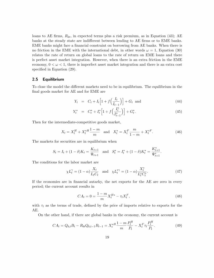
2.5 Equilibrium

To close the model the different markets need to be in equilibrium. The equilibrium in thefinal goods market for AE and for EME are

Yt = Ct + It

[1 + f

( ItIt−1

)]+Gt and (44)

Y ∗t = C∗t + I∗t

[1 + f

( I∗tI∗t−1

)]+G∗t . (45)

Then for the intermediate-competitive goods market,

Xt = XHt +X∗Ht

1−mm

and X∗t = XFt

m

1−m+X∗Ft . (46)

The markets for securities are in equilibrium when

St = It + (1− δ)Kt =Kt+1

Ψt+1and S∗t = I∗t + (1− δ)K∗t =

K∗t+1

Ψ∗t+1

.

The conditions for the labor market are

χLγt = (1− α)Xt

LtCtand χL∗γt = (1− α)

X∗tL∗tC

∗t

. (47)

If the economies are in financial autarky, the net exports for the AE are zero in everyperiod; the current account results in

CAt = 0 =1−mm

XH∗t − τtXF

t , (48)

with τt as the terms of trade, defined by the price of imports relative to exports for theAE.

On the other hand, if there are global banks in the economy, the current account is

CAt = Qb,tBt −RbtQb,t−1Bt−1 = X∗Ht1−mm

PHtPt−XF

t τtPHtPt

. (49)

19

The global asset is in zero net supply, as a result

Bt = B∗t1−mm

. (50)

To close the model the last conditions correspond to the riskless debt. Total householdsavings equal total deposits plus government debt. Government debt is perfect substituteof deposits to banks,

Dht = Dt +Dgt and Dh∗

t = D∗t +D∗gt. (51)

We formally define the equilibrium of the banking model in Appendix B.

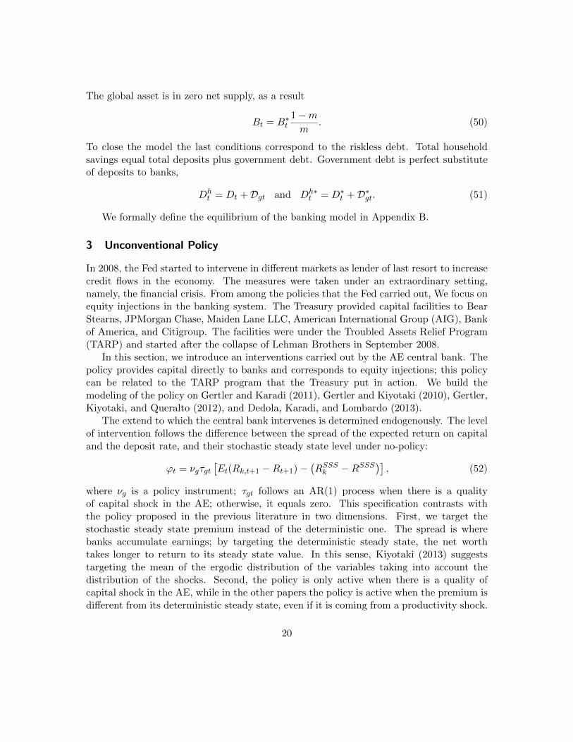
3 Unconventional Policy

In 2008, the Fed started to intervene in different markets as lender of last resort to increasecredit flows in the economy. The measures were taken under an extraordinary setting,namely, the financial crisis. From among the policies that the Fed carried out, We focus onequity injections in the banking system. The Treasury provided capital facilities to BearStearns, JPMorgan Chase, Maiden Lane LLC, American International Group (AIG), Bankof America, and Citigroup. The facilities were under the Troubled Assets Relief Program(TARP) and started after the collapse of Lehman Brothers in September 2008.

In this section, we introduce an interventions carried out by the AE central bank. Thepolicy provides capital directly to banks and corresponds to equity injections; this policycan be related to the TARP program that the Treasury put in action. We build themodeling of the policy on Gertler and Karadi (2011), Gertler and Kiyotaki (2010), Gertler,Kiyotaki, and Queralto (2012), and Dedola, Karadi, and Lombardo (2013).

The extend to which the central bank intervenes is determined endogenously. The levelof intervention follows the difference between the spread of the expected return on capitaland the deposit rate, and their stochastic steady state level under no-policy:

ϕt = νgτgt[Et(Rk,t+1 −Rt+1)−

(RSSSk −RSSS

)], (52)

where νg is a policy instrument; τgt follows an AR(1) process when there is a qualityof capital shock in the AE; otherwise, it equals zero. This specification contrasts withthe policy proposed in the previous literature in two dimensions. First, we target thestochastic steady state premium instead of the deterministic one. The spread is wherebanks accumulate earnings; by targeting the deterministic steady state, the net worthtakes longer to return to its steady state value. In this sense, Kiyotaki (2013) suggeststargeting the mean of the ergodic distribution of the variables taking into account thedistribution of the shocks. Second, the policy is only active when there is a quality ofcapital shock in the AE, while in the other papers the policy is active when the premium isdifferent from its deterministic steady state, even if it is coming from a productivity shock.

20

We assume that τgt = ρτgτgt−1 +εΨ,t, where εΨ,t is the same exogenous variable that drivesthe AE quality of capital shock.

The policies are carried out only by the policy maker of the country directly hit by theshock. Next, we describe the policy.

3.1 Equity Injection

Under this policy, the central bank gives funds to AE banks and the banks then decidehow to allocate these extra resources optimally. The quantity of funds that the governmentprovides is a fraction of the total assets of AE banks, Ngt = ϕtQtSt. The net worth of theAE banking system is set to be

Nt = (σ + ξ) [Zt + (1− δ)Qt]Kt − σRtDt−1 − σRbtQbt−1Bt−1 − σRgtNg,t−1.

Redefining Equation (37) yields

QtSt = φtNt +Ngt +QbtBt. (53)

The interest rate paid to the government is equal to the interest rate on capital.

3.2 Government

Consolidating monetary and fiscal policy, total government expenditure is the sum of con-sumption, Gt, loans to firms, Sgt (or total intervention), and debt issued last period,RtDgt−1. Government resources are lump sum taxes, Tt, new debt issued, Dgt, and thereturn on the intervention that the government made last period. The budget constraintof the consolidated government is

Gt +Ngt +RtDgt−1 = Tt +Dgt + σRgtNg,t−1.

The debt that government issues is a perfect substitute of the deposits to banks, there-fore, the rate that they pay is the same and households are indifferent between lendingto banks and to the government. Government expenditure includes a constant fraction oftotal output and a cost for each unit of intervention issued,

Gt = τ1SNgt + τ2SN 2gt + gY.

The efficiency cost are quadratic on the intervention of the central bank, as in Gertler,Kiyotaki, and Queralto (2012).

4 Macro-prudential Policy

The consequences of the financial crisis brought back the discussion regarding macro-prudential regulation. The financial crisis reminded policymakers around the globe about

21

the costs of a systemic disruption in financial markets. Macro-prudential regulation aims toreduce the systemic risk of the financial system. The International Monetary Fund (2011)considers two types of macro-prudential tools: (1) instruments designed to control thesystemic risk across time and across individual institutions and (2) instruments that canbe re-calibrated according to specific objectives and with the purpose of reducing systemicrisk. Complementary, the BIS (2010a) defines a macro-prudential tool as the one that itsmain objective is to promote the stability of the financial system as a whole.

Many EME implemented macro-prudential regulation at the end of the 90s due to sev-eral EME crisis. The tools that EME have been using are mainly of the type (2) of theIMF, i.e. flexible instruments that vary according to the different systemic risks, Castillo,Quispe, Contreras, and Rojas (2011). EMEs have strengthening the regulatory frameworkwith respect to maturity mistmatches on the balance sheets of financial institutions, limitshort-term foreign borrowing, and strengthening the supervision of foreign currency expo-sures. These measures have ensured a resilient financial system. (BIS, 2010b)

In Mexico after the so called Tequila Crisis in 1995, the Bank of Mexico started toimplement macro-prudential regulation. One of the main changes in the regulation wasto require global banks offering banking services in Mexico to do it through subsidiaries,instead of branches. Subsidiaries are separate entities from their parent bank with theirown capital. By doing this, Citibank, Santander, BBVA, HSBC, and Scotiabank arrivedto a very regulated market where foreign and domestic banks have the same rules andsupervisor processes.

Among the macro-prudential regulation that the Mexican financial system implementedin the 90s are: regulation for banks’ foreign currency operations (maturity and currency);a cap on exposure to related counterparties; caps on interbank exposures and higher lim-its on value at risk for pension fund portfolios at times of high volatility, among others.(Guzman Calafell, 2013). The macro-prudential measures implemented in the 90s helpedMexican banks to be resilience during the financial crisis. With the financial crisis andthe Basel III Agreement, some new measures were implemented and there is still room forworking more on targeting the sources of instability of the financial system.

Since October 2010, the Bank of Korea has introduced two macro-prudential measuresto address the risk factors of capital inflows and outflows generated on the demand and thesupply side. First, they introduced leverage caps on banks’ foreign exchange derivativespositions. The aim was to curb the increase in banks’ short-term external debt and the cur-rency and maturity mismatches. Later on, they introduced the macro-prudential stabilitylevy. The objective was to reduce the increase in banks’ non-core liabilities (non-depositforeign currency liabilities). The levy rates varies according to the maturity of the liability.The effects contributed to reduce banks’ foreign borrowings and improving their maturitystructures. (Kim, 2014 and Shin, 2010)

In this section, we introduce one possible macro-prudential tool in line with the Koreanexperience. In the framework that we have developed in this paper, the systemic risk orthe contagion across financial institutions for the EME comes from the international asset.

22

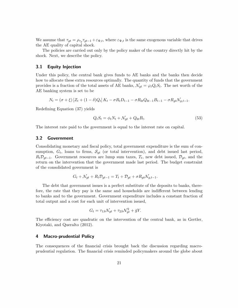
Moreover, the international contagion is deeper when there is a friction for EME banks onobtaining funds from AE banks because the former can run away with part of the interna-tional asset, i.e. 0 < ω < 1. This is exactly the friction that the macro-prudential policytargets because is the source of financial instability for the EME.

The policy is a tax on deviations from the steady state of the ratio of the global assetwith the EME banks’ capital,

ϑ∗gt = τ∗g

(Q∗btB

∗t

N∗t−Q∗bB

∗

N∗

)2

. (54)

How big the tax is has an exogenous (arbitrary) component τ∗g and an endogenous onethat corresponds to the brackets. In Section 5.4 we do a welfare analysis for the differentlevels of τ∗g . The tax goes directly into the incentive compatibility constraint, Equation(28), changing the perception of how risky EME banks are for AE banks. Therefore, theconstraint with the policy becomes

Vt(s∗t , b∗t , d∗t ) ≥ θ∗

[Q∗t s

∗t − (1 + ϑ∗gt)ωQ

∗btb∗t

]. (55)

When the value of the ratio moves away from its steady state, the tax becomes positive andbanks are perceived as with a lower friction because of the macro-prudential policy. Nomatter in which direction, EME banks are perceived as safer due to the policy. Quantitiesmove smoother with the policy because of this adjustment cost.

The net worth of EME banks becomes

N∗t = (σ∗ + ξ∗)R∗ktQ∗t−1S

∗t−1 − σ∗

[R∗tD

∗t−1 + (1 + ϑ∗gt)R

∗btQ∗b,t−1B

∗t−1

].

Finally, the government budget constraint of the EME is

G∗t = T ∗t +D∗gt + ϑ∗gtQ∗btB∗t .

In this framework, the macro-prudential policy helps to limit currency exposures arisingfrom cross-border banking flows and limits adverse consequences associated with them. Thepolicy has a levy on non-core liabilities, as the Korean experience. This is in line with BIS(2010b)’s suggestions regarding macro-prudential measures in EMEs.

5 Crisis experiment

In this section, we present numerical experiments to show how the model captures keyaspects of the international transmission of a financial crisis. First, we present the cali-bration; next, we analyze a crisis experiment without response from the government andwe highlight the role of the foreign debt in the transmission of the crisis and how it worksas insurance for the economy that is hit by a shock. Next, we study how credit marketintervention by the AE central bank can mitigate the effects of the crisis. Finally, welook at macro-prudential policy carried out by the EME and its combination with theunconventional monetary policy of the AE.

23

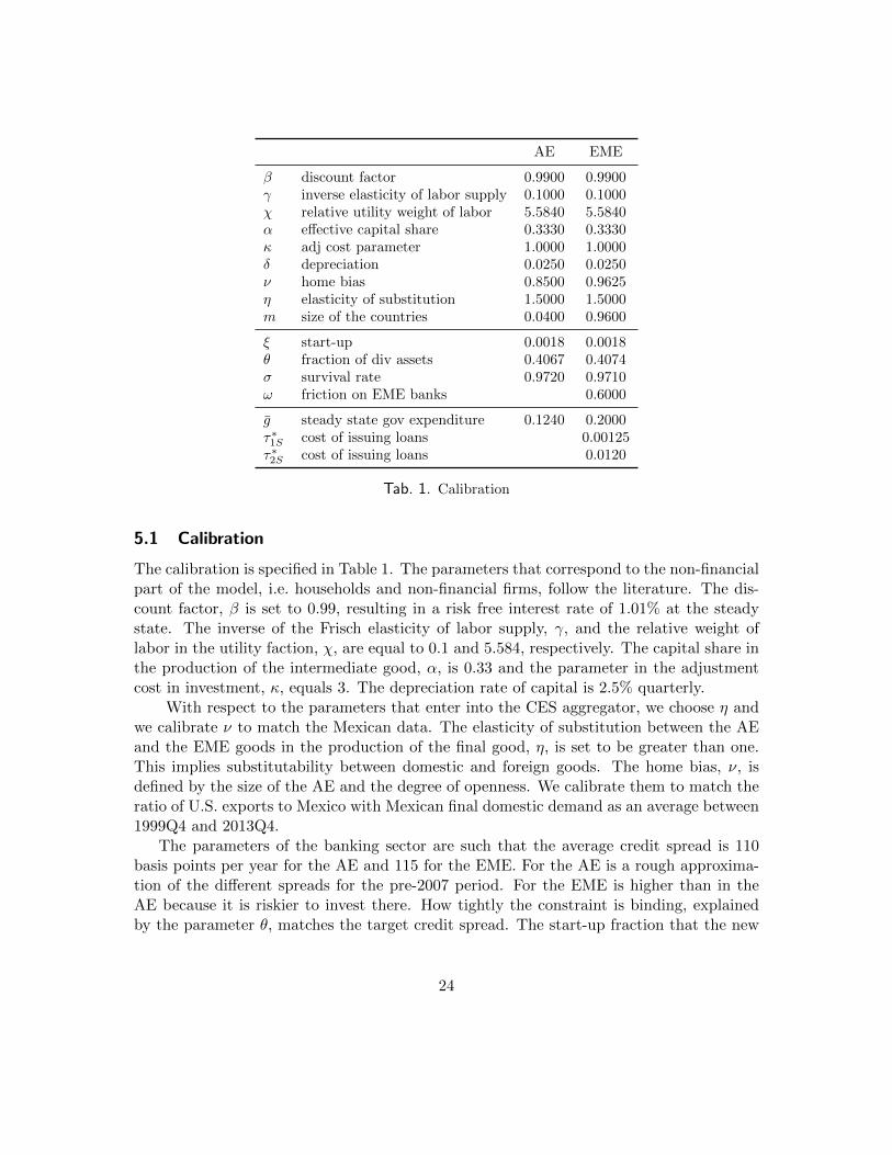
AE EME

β discount factor 0.9900 0.9900γ inverse elasticity of labor supply 0.1000 0.1000χ relative utility weight of labor 5.5840 5.5840α effective capital share 0.3330 0.3330κ adj cost parameter 1.0000 1.0000δ depreciation 0.0250 0.0250ν home bias 0.8500 0.9625η elasticity of substitution 1.5000 1.5000m size of the countries 0.0400 0.9600

ξ start-up 0.0018 0.0018θ fraction of div assets 0.4067 0.4074σ survival rate 0.9720 0.9710ω friction on EME banks 0.6000

g steady state gov expenditure 0.1240 0.2000τ∗1S cost of issuing loans 0.00125τ∗2S cost of issuing loans 0.0120

Tab. 1. Calibration

5.1 Calibration

The calibration is specified in Table 1. The parameters that correspond to the non-financialpart of the model, i.e. households and non-financial firms, follow the literature. The dis-count factor, β is set to 0.99, resulting in a risk free interest rate of 1.01% at the steadystate. The inverse of the Frisch elasticity of labor supply, γ, and the relative weight oflabor in the utility faction, χ, are equal to 0.1 and 5.584, respectively. The capital share inthe production of the intermediate good, α, is 0.33 and the parameter in the adjustmentcost in investment, κ, equals 3. The depreciation rate of capital is 2.5% quarterly.

With respect to the parameters that enter into the CES aggregator, we choose η andwe calibrate ν to match the Mexican data. The elasticity of substitution between the AEand the EME goods in the production of the final good, η, is set to be greater than one.This implies substitutability between domestic and foreign goods. The home bias, ν, isdefined by the size of the AE and the degree of openness. We calibrate them to match theratio of U.S. exports to Mexico with Mexican final domestic demand as an average between1999Q4 and 2013Q4.

The parameters of the banking sector are such that the average credit spread is 110basis points per year for the AE and 115 for the EME. For the AE is a rough approxima-tion of the different spreads for the pre-2007 period. For the EME is higher than in theAE because it is riskier to invest there. How tightly the constraint is binding, explainedby the parameter θ, matches the target credit spread. The start-up fraction that the new

24

banks receive, ξ, is 0.18% of the last period’s assets, which corresponds to the value usedby Gertler and Kiyotaki (2010) and is equal for both economies. AE banks lend to EMEbanks because the survival rate is different across countries, 0.972 for AE and 0.971 forEME banks. On average, AE banks survive 8 years, while EME banks around 7 years.Atthe steady state, the holding of global asset represents 1.4% of the total assets of the AEbanks, which matches the data for total lending by U.S. banks to Mexican counterpartiesfrom the year 1999Q4 until 2013Q4, and constitutes 7.8% of Mexican banks’ total assets.We assume a negative i.i.d. shock that occurs in the AE.

5.2 No policy response

5.2.1 Safety EME Banks ω = 1

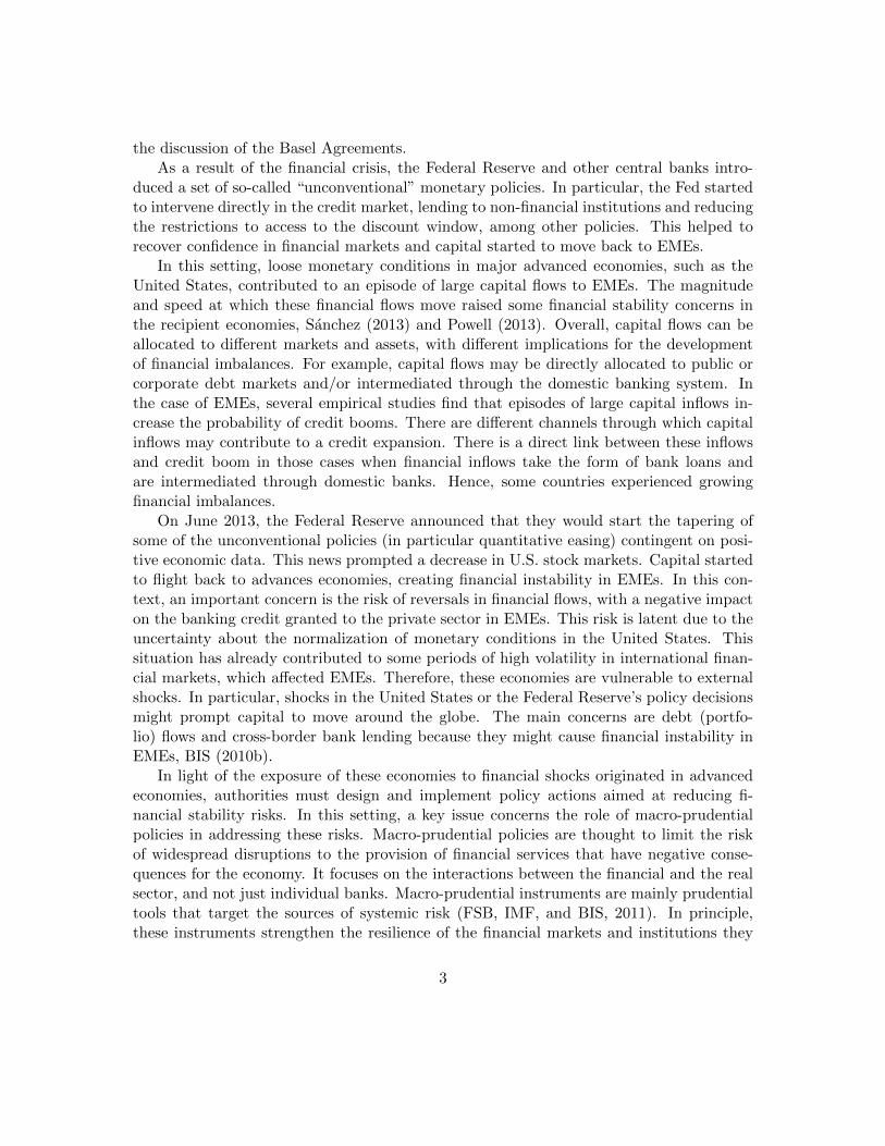
Figure 3 shows the impulse responses to a decline in the AE quality of capital of 5% inperiod t comparing three models. The first model is one without financial frictions and infinancial autarky and is the green thick dash-dotted line. The second model has financialfrictions but no trade in assets, and is the blue solid line. The financial frictions are a laGertler and Kiyotaki (2010). The third model is with financial frictions and an interna-tional debt market (financial openness) with no further EME frictions (ω = 1); it is the redthin dashed line. The comparison of these models shows how the transmission mechanismacross countries changes given the different assumptions. In the first two models, there isonly international spillover due to the trade of intermediate goods. In the third model, weadd the international financial mechanism. The comparison helps us understanding theinsurance and the transmission role of the international debt market. In Appendix D, weshow the complete set of impulse responses functions: AE and EME variables are in Figure8.

When there is a decrease in the AE quality of capital, and there are no financialfrictions (i.e. no banks) in the economy, all the resources are channeled to recovering fromthe initial shock. Investment and asset price go up. Households cut down on consumptionon impact because of lower labor income. Final domestic demand and production at theAE fall because of the negative shock.

The AE cuts back not only the demand for local goods, XHt , but also imports, XF

t .There are fewer AE goods in the economy because of the shock. As a result, every unit ofAE good is more expensive and the terms of trade slightly improve (deteriorate) for theAE (EME). The trade balance is defined by Equation (48) and equals zero in every periodbecause there is no international borrowing/lending.

The AE demand of EME goods decreases but the EME starts demanding more ofdomestic products because they are relatively cheaper. The EME increases its produc-tion, X∗t , while substituting advanced for domestic goods. Nevertheless, consumption andinvestment decrease because the interest rate is higher. In the model without financialfrictions and in financial autarky, there is no international co-movement either in asset

25

0 20 40−1

−0.5

0EME Capital (K*)

0 20 40−2

−1

0

1EME Asset Price (Q*)

0 20 40−6

−4

−2

0EME Net Worth (N*)

0 20 40−4

−2

0

2EME Investment (I*)

0 20 40−1

−0.5

0

0.5EME Consumption (C*)

global banks ω=1banks and fin autarkybenchmark

0 20 40−0.1

0

0.1

EME Premium E(Rk)*−R*

0 20 40−4

−2

0

2Terms of Trade

0 20 40−10

−5

0Global Asset (B*)

0 20 40−2

−1

0

1

Global Asset Price (Qb* )

0 20 40−30

−20

−10

0AE Net Worth (N)

0 20 40−6

−4

−2

0AE Capital (K)

0 20 40−5

0

5AE Investment (I)

0 20 40−4

−2

0

2AE Asset Price (Q)

0 20 40−2

−1

0AE Consumption (C)

0 20 400

0.5

1

AE Premium E(Rk)−R

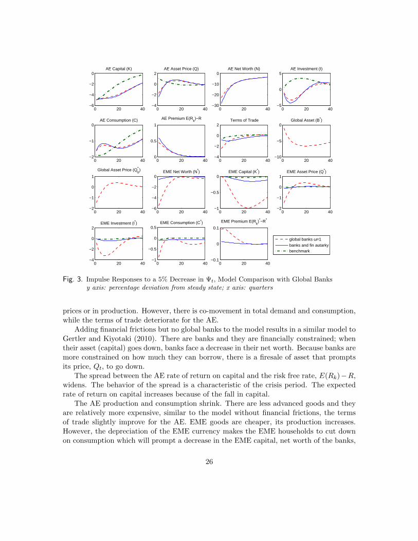
Fig. 3. Impulse Responses to a 5% Decrease in Ψt, Model Comparison with Global Banksy axis: percentage deviation from steady state; x axis: quarters

prices or in production. However, there is co-movement in total demand and consumption,while the terms of trade deteriorate for the AE.

Adding financial frictions but no global banks to the model results in a similar model toGertler and Kiyotaki (2010). There are banks and they are financially constrained; whentheir asset (capital) goes down, banks face a decrease in their net worth. Because banks aremore constrained on how much they can borrow, there is a firesale of asset that promptsits price, Qt, to go down.

The spread between the AE rate of return on capital and the risk free rate, E(Rk)−R,widens. The behavior of the spread is a characteristic of the crisis period. The expectedrate of return on capital increases because of the fall in capital.

The AE production and consumption shrink. There are less advanced goods and theyare relatively more expensive, similar to the model without financial frictions, the termsof trade slightly improve for the AE. EME goods are cheaper, its production increases.However, the depreciation of the EME currency makes the EME households to cut downon consumption which will prompt a decrease in the EME capital, net worth of the banks,

26

and the asset price. Asset prices and production co-move across countries. Although thereis a larger spillover to the EME economy with financial frictions than without them, thetransmission is still negligible.

When we allow for foreign debt, AE banks lend to EME banks. EME banks borrowinternationally; AE banks diversify their assets and pool a country specific shock. Theseasset market characteristics have been discussed by Cole and Obstfeld (1991) and Cole(1993).

The decrease in the value of assets and securities in the AE prompts AE banks to bemore financially constrained. The reaction is similar to the model without global banksand is shown by the solid-blue and the thick dashed-red line in Figure 3. The mechanismthat takes place for the AE variables is the same in both models with financial frictions.However, final domestic demand is less affected by the shock when there are global banksbecause the AE can partially pool the country specific shock.

In this model ω = 1, the return on EME assets equalizes the return on EME debt.EME banks face a reduction in their net worth because of a country specific shock in theAE. EME financial intermediaries are more financially constrained and reduce lending todomestic businesses. Investment and the price of capital shrink. The global banks transmitthe crisis from the AE to the EME.

Two types of spillovers disturb the EME: the demand and the international debt ef-fects. The demand effect prompts an increase in production because the exchange rate isdepreciating. The international debt effect generates a tightening of the EME borrowingconstraint because there is a decrease in the value of international lending. The interna-tional debt effect predominates and the net worth of EME banks falls and households cutdown on consumption. The effect on production vanishes after 3 periods. Global banksimply financial openness, the current account is now defined in Equation (49).

In a model with global banks and financial frictions, the AE and EME consumption,asset price, and total demand co-move, while production does not (on impact). The assetmarkets across countries are integrated when ω = 1 because of the equalization of returnsof the asset market in the AE and the EME. For AE banks lending to EME banks onlyimply a country specific premium, but they do not imply a risk.

5.2.2 Risky EME banks 0 < ω < 1

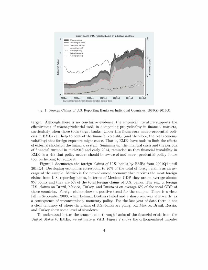
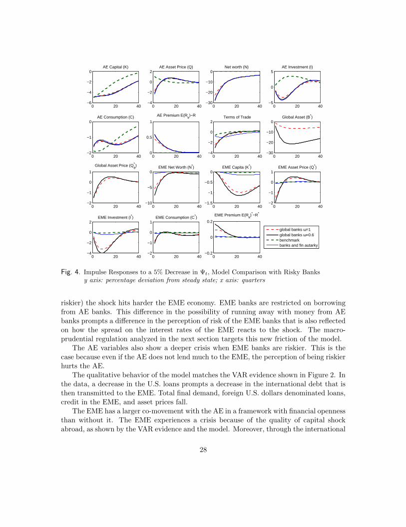
In Figure 4 we compare two models. They differ on the level of riskiness of EME bankswith respect to the international asset. The red dashed line is the same model as in Figure3, the AE banks perceive the EME banks as safe, ω = 1. The black full line is a modelin which EME banks are riskier, 0 < ω < 1. Given that the small economy is an EME,it is plausible to assume that EME banks are riskier. Figure 9 in Appendix D shows thecomplete set of AE and EME variables.

The economies show a similar reaction in both cases to an AE quality of capital shock.However, when EME banks can run away with money from AE banks (when EME banks are

27

0 20 40−10

−5

0EME Net Worth (N*)

0 20 40−1.5

−1

−0.5

0EME Capita (K*)

0 20 40−2

−1

0

1EME Asset Price (Q*)

0 20 40−4

−2

0

2EME Investment (I*)

0 20 40−2

−1

0

1EME Consumption (C*)

0 20 40−0.2

0

0.2

EME Premium E(Rk)*−R*

global banks ω=1global banks ω=0.6benchmarkbanks and fin autarky

0 20 40−30

−20

−10

0Global Asset (B*)

0 20 40−2

−1

0

1

Global Asset Price (Qb* )

0 20 40−6

−4

−2

0AE Capital (K)

0 20 40−4

−2

0

2AE Asset Price (Q)

0 20 40−30

−20

−10

0Net worth (N)

0 20 40−5

0

5AE Investment (I)

0 20 40−2

−1

0AE Consumption (C)

0 20 400

0.5

1

AE Premium E(Rk)−R

0 20 40−4

−2

0

2Terms of Trade

Fig. 4. Impulse Responses to a 5% Decrease in Ψt, Model Comparison with Risky Banksy axis: percentage deviation from steady state; x axis: quarters

riskier) the shock hits harder the EME economy. EME banks are restricted on borrowingfrom AE banks. This difference in the possibility of running away with money from AEbanks prompts a difference in the perception of risk of the EME banks that is also reflectedon how the spread on the interest rates of the EME reacts to the shock. The macro-prudential regulation analyzed in the next section targets this new friction of the model.

The AE variables also show a deeper crisis when EME banks are riskier. This is thecase because even if the AE does not lend much to the EME, the perception of being riskierhurts the AE.

The qualitative behavior of the model matches the VAR evidence shown in Figure 2. Inthe data, a decrease in the U.S. loans prompts a decrease in the international debt that isthen transmitted to the EME. Total final demand, foreign U.S. dollars denominated loans,credit in the EME, and asset prices fall.

The EME has a larger co-movement with the AE in a framework with financial opennessthan without it. The EME experiences a crisis because of the quality of capital shockabroad, as shown by the VAR evidence and the model. Moreover, through the international

28

debt market, the AE manages to partially insure itself against the shock. The EMEexperiences a deeper financial crisis when domestic banks can run away with resourcesfrom the AE banks.

5.3 Policy response

5.3.1 Unconventional Monetary Policy

We analyze equity injections. The policy are carried out only by the AE central bank.One of the reasons that motivated the Fed to intervene was the abnormal credit spread inseveral markets. In this sense, the central bank determines the fraction of private creditto intermediate by following the difference between the risky and the risk free interest rateand its stochastic steady state value, as in Equation (52).

Figure 5 shows a small set of variables with the results; Figure 10 in Appendix D showsmore variables. The solid black line is the model with financial frictions and financialopenness without policy with risky banks, the same as in the previous figure. The dashedblue line is the model with equity injections. The policy parameter ν∗g is set to be 10000 andρτ∗g = 0.66. The costs of issuing government loans follow Gertler, Kiyotaki, and Queralto(2012) and the fraction of government expenditure at the steady state matches the datafor the United States and Mexico.

The central bank intervention prompts a higher price of the domestic asset than underno intervention. The initial intervention is around 3% of total AE assets. Higher assetprice implies that AE banks are less financially constrained. The AE banks’ net worthfalls almost 10% less than under no-policy. The asset price is also the price of investment,therefore, investment contraction is lower with the policy. Consumers pay the cost of thepolicy.

Because of some level of asset market integration, the price of the global asset also fallsless. EME banks are less financially constrained than under no policy, the net worth ofEME banks drops only 3% on impact. Banks lend more to domestic firms; as a result,the EME asset price decreases by less with the AE policy and the fall in investment issmoothed.

In conclusion, with AE equity injections the advanced and the emerging economies get asmoother impact of the crisis. Although EME banks do not have direct access to the policy,the EME profits through the higher prices in the interbank market. EME consumptionand total demand drop less than under no-policy.

5.3.2 Macro-prudential Policy

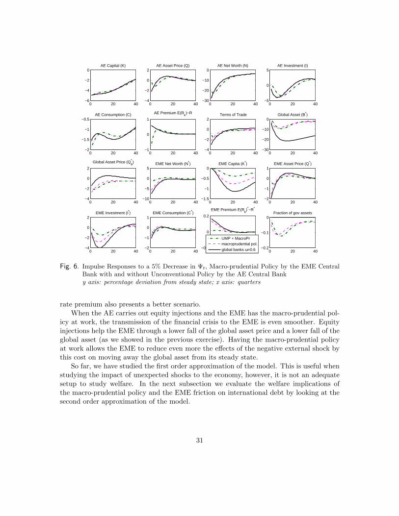
In this part, we analyze the effects of the EME macro-prudential policy. In particular,we look at three models. Figure 6 shows a small set of variable. The black solid line isthe same model without policy with risky banks shown in previous figures. The magentadashed line is a model with the quality of capital shock in the AE and macro-prudential

29

0 20 40−1.5

−1

−0.5

0EME Capita (K*)

0 20 40−2

−1

0

1EME Asset Price (Q*)

0 20 40−10

−5

0

5EME Net Worth (N*)

0 20 40−4

−2

0

2EME Investment (I*)

0 20 40−2

−1

0

1EME Consumption (C*)

0 20 40−0.2

0

0.2

EME Premium E(Rk)*−R*

UMP

global banks ω=0.6

0 20 40−6

−4

−2

0AE Capital (K)

0 20 40−4

−2

0

2AE Asset Price (Q)

0 20 40−30

−20

−10

0AE Net Worth (N)

0 20 40−5

0

5AE Investment (I)

0 20 40−2

−1.5

−1

−0.5AE Consumption (C)

0 20 40−1

0

1

AE Premium E(Rk)−R

0 20 40−4

−2

0

2Terms of Trade

0 20 40−30

−20

−10

0Global Asset (B*)

0 20 40−2

−1

0

1

Global Asset Price (Qb* )

0 20 400

2

4Fraction of gov assets

Fig. 5. Impulse Responses to a 5% Decrease in Ψt, Unconventional Policies by AE Central Banky axis: percentage deviation from steady state; x axis: quarters

policy in the EME. The green dotted-dashed line is the model with macro-prudential policycarried out by the EME and unconventional policy (equity injections) carried out by theAE. The parameters of the unconventional policy are the same as in the previous exercise.For the macro-prudential policy, the calibrated parameter is set to 2000. In Appendix D,Figure 11 we show the rest of the variables.

The macro-prudential intervention targets the ratio between the holdings of cross-border banking flows by EME banks (the non-core liabilities) and the EME banks’ capital.The fact of having the tax makes the AE banks perceived EME banks as safer; moreoverthere is a cost on moving away from the steady state, so the international asset quantitiesreact much less with the macro-prudential policy than without it.

If the EME implements the macro-prudential policy (the magenta dashed line) theglobal asset is costly to move and so the transmission of the external shock is smaller.Moreover, the net worth of the domestic banks fall less, which prompts loans and capitalto be cut by less. The price of the capital doesn’t fall as much and so investment moves ina smoother way. Even the household’s consumption shows a smaller reaction. The interest

30

0 20 40−1.5

−1

−0.5

0EME Capita (K*)

0 20 40−2

−1

0

1EME Asset Price (Q*)

0 20 40−10

−5

0

5EME Net Worth (N*)

0 20 40−4

−2

0

2EME Investment (I*)

0 20 40−2

−1

0

1EME Consumption (C*)

0 20 40−0.2

0

0.2

EME Premium E(Rk)*−R*

UMP + MacroPrmacroprudential pol.

global banks ω=0.6

0 20 40−6

−4

−2

0AE Capital (K)

0 20 40−4

−2

0

2AE Asset Price (Q)

0 20 40−30

−20

−10

0AE Net Worth (N)

0 20 40−5

0

5AE Investment (I)

0 20 40−2

−1.5

−1

−0.5AE Consumption (C)

0 20 40−1

0

1

AE Premium E(Rk)−R

0 20 40−4

−2

0

2Terms of Trade

0 20 40−30

−20

−10

0Global Asset (B*)

0 20 40−4

−2

0

2

Global Asset Price (Qb* )

0 20 40−0.2

−0.1

0Fraction of gov assets

Fig. 6. Impulse Responses to a 5% Decrease in Ψt, Macro-prudential Policy by the EME CentralBank with and without Unconventional Policy by the AE Central Banky axis: percentage deviation from steady state; x axis: quarters

rate premium also presents a better scenario.When the AE carries out equity injections and the EME has the macro-prudential pol-

icy at work, the transmission of the financial crisis to the EME is even smoother. Equityinjections help the EME through a lower fall of the global asset price and a lower fall of theglobal asset (as we showed in the previous exercise). Having the macro-prudential policyat work allows the EME to reduce even more the effects of the negative external shock bythis cost on moving away the global asset from its steady state.

So far, we have studied the first order approximation of the model. This is useful whenstudying the impact of unexpected shocks to the economy, however, it is not an adequatesetup to study welfare. In the next subsection we evaluate the welfare implications ofthe macro-prudential policy and the EME friction on international debt by looking at thesecond order approximation of the model.

31

5.4 Welfare analysis

In this part, we introduce consumers’ welfare. We want to look at the advanced andemerging consumers’ welfare given the different level of riskiness of EME banks, i.e. ω, andthe level of intervention of the EME macro-prudential policy through the policy parameterτ∗g .

The welfare criterion considered here is the one used by Gertler and Karadi (2011) anddeveloped by Faia and Monacelli (2007). The household’s welfare function is given by

Welf t = U(Ct, Lt) + βEtWelf t+1, (56)

where the utility function comes from Equation (6). Welfare is defined as the lifetimeutility of the consumers. We compare the different calibrations using the consumptionequivalent, i.e. the fraction of household consumption that would be needed to equate thewelfare of the deterministic steady state to the welfare under policy, in the case of themacro-prudential intervention.

The stochastic steady state is defined as the place where the model stands after 500periods given the deterministic steady state as starting point. The approximation of themodel is of the second order. We don’t give shocks in the process of going through thedeterministic to the stochastic steady state but the variance of the perturbations are takeninto account in the solution of the model. We follow Carrillo, Peersman, and Wauters(2013) on the way to calculate the stochastic steady state and Schmitt-Grohe and Uribe(2007) for the definition of consumption equivalent.

The consumption equivalent for the different levels of risky EME banks are in the leftpanel of Figure 7. We plot the consumption equivalent for the advance and the emergingeconomies when there are only quality of capital shocks in the AE (red thin dashed lineand black thin solid line, respectively) and when there are quality of capital, governmentexpenditure, and productivity shocks in both economies (green thick dashed line and bluethick solid line, respectively) . The distribution of technology and government shocks followSchmitt-Grohe and Uribe (2005). Technology shocks have an autoregressive coefficient of0.8556 and a standard deviation of 0.0064; the autoregressive coefficient of governmentexpenditure shocks and the standard deviation are 0.87 and 0.016, respectively.

The different levels of ω reveal that to quality of capital shocks in the AE, EMEconsumers are better off because they do not get the impact of the shock directly. AEconsumers decrease there consumption much more than the decrease in labor. Moreover, ahigher exposure to cross-border banking flows (higher ω) makes EME consumers worse off.This is the case because the EME is more exposed to foreign debt when EME banks areless risky (higher ω). Therefore, the terms of trade get worsen with higher values of ω dueto the shock and EME households have to work more. On the other hand, the depreciationof the terms of trade for the EME implies an appreciation for the AE, so the households ofthe latter are better off with higher level of riskiness of EME banks. When the EME bankshave very little risk for the AE banks, AE households are better off with domestic quality of

32

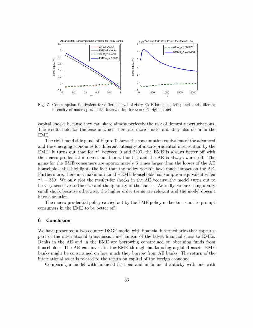
0 0.2 0.4 0.6 0.8 1−0.2

0

0.2

0.4

0.6

0.8

1

1.2AE and EME Consumption Equivalents for Risky Banks

ω

cons

. equ

iv. (

%)

AE all shocksEME all shocksAE σΨ= 0.0005

EME σΨ= 0.0005

0 500 1000 1500 2000−1

0

1

2

3

4

5x 10

−5AE and EME Con. Equiv. for MacroPr. Pol.

τ*

cons

. equ

iv. (

%)

AE σΨ= 0.000025

EME σΨ= 0.000025

Fig. 7. Consumption Equivalent for different level of risky EME banks, ω -left panel- and differentintensity of macro-prudential intervention for ω = 0.6 -right panel-

capital shocks because they can share almost perfectly the risk of domestic perturbations.The results hold for the case in which there are more shocks and they also occur in theEME.

The right hand side panel of Figure 7 shows the consumption equivalent of the advancedand the emerging economies for different intensity of macro-prudential intervention by theEME. It turns out that for τ∗ between 0 and 2200, the EME is always better off withthe macro-prudential intervention than without it and the AE is always worse off. Thegains for the EME consumers are approximately 6 times larger than the looses of the AEhouseholds; this highlights the fact that the policy doesn’t have much impact on the AE.Furthermore, there is a maximum for the EME households’ consumption equivalent whenτ∗ = 350. We only plot the results for shocks in the AE because the model turns out tobe very sensitive to the size and the quantity of the shocks. Actually, we are using a verysmall shock because otherwise, the higher order terms are relevant and the model doesn’thave a solution.

The macro-prudential policy carried out by the EME policy maker turns out to promptconsumers in the EME to be better off.

6 Conclusion

We have presented a two-country DSGE model with financial intermediaries that capturespart of the international transmission mechanism of the latest financial crisis to EMEs.Banks in the AE and in the EME are borrowing constrained on obtaining funds fromhouseholds. The AE can invest in the EME through banks using a global asset. EMEbanks might be constrained on how much they borrow from AE banks. The return of theinternational asset is related to the return on capital of the foreign economy.

Comparing a model with financial frictions and in financial autarky with one with

33

a global interbank market suggests that the latter generates a higher co-movement ofthe crisis that matches qualitatively the behavior seen in the data, as shown in the VARanalysis. When a quality of capital shock hits the AE, AE and EME experience a crisis bothin real and financial variables. The global asset prompts the international transmission.The net worth of EME banks drops because the price of the international asset falls andso does the quantities. EME banks face a reduction in their liabilities and they are moreconstrained to lend to domestic non-financial firms. The price of EME domestic assetsdrops prompting a fall in investment, consumption, and total demand. When EME arealso constrained on how much they can borrow from AE banks, the crisis is deeper in theEME in comparison to the case in which there is no friction on borrowing AE banks.

Banks that intermediate funds across borders and in different currencies entail relevantchallenges in terms of policy and regulation. For EMEs capital flows volatility have aparticular interest. We study the introduction of a macro-prudential policy by the CentralBank of the EME with the objective of reducing the financial and real variables volatilitythat cross-border bank capital might prompt. The policy is effective on smoothing theimpact of external shock because it targets directly one of the frictions that makes thetransmission deeper, i.e. the likelihood of EME banks running away with loans from AEbanks. Moreover, the policy makes EME consumers better off. The macro-prudentialpolicy is also effective on reducing the volatility of EME variables when the AE carries outunconventional monetary policy, in particular equity injections.

The paper focuses on one aspect of the transmission mechanism of the financial crisisfor EMEs: the cross-border bank capital. Banks that intermediate funds across bordersand in different currencies imply relevant challenges in terms of policy and regulation,especially for EMEs. One tool that these economies have to create a resilience financialsystem is macro-prudential policy. In future research, we are planning to extend the modelto agency problems when banks lend to non-financial firms, with particular interest onEMEs. Moreover, the macro-prudential policy has many possible instruments that haven’tbeen studied in this paper and that are of relevance for policy makers.

In the model, the AE can only invest in the EME through the banks. We only lookat the cross-border bank capital. In reality, non-financial firms issue dollar denominateddebt that for the case of Mexico is of extreme relevance. This makes the cross-countryrelation much more complicated. We believe that this model captures one aspect of thecross-country relations that helps to understand the risks of external shocks for EMEs.

References

BIS (2010a): “Macroprudential policy and addressing procyclicality,” in 80th Annual Re-port.

(2010b): “Post-crisis policy challenges in emerging market economies,” in 80thAnnual Report.

34

Carrillo, J. A., G. Peersman, and J. Wauters (2013): “Endogenous Wage Indexa-tion and Aggregate Shocks,” Working Papers 2013-19, Banco de Mxico.

Castillo, P., Z. Quispe, A. Contreras, and Y. Rojas (2011): “Polıtica macro-prudencial en los paıses de la region,” Revista Moneda, 149, 4–7.

Christiano, L. J., M. Eichenbaum, and C. L. Evans (2005): “Nominal Rigiditiesand the Dynamic Effects of a Shock to Monetary Policy,” Journal of Political Economy,113(1), 1–45.

Cole, H. (1993): “The macroeconomic effects of world trade in financial assets,” QuarterlyReview, 28(Summer), 12–21.

Cole, H., and M. Obstfeld (1991): “Commodity trade and international risk sharing:How much do financial markets matter?,” Journal of Monetary Economics, 28(1), 3 –24.

Dedola, L., P. Karadi, and G. Lombardo (2013): “Global implications of nationalunconventional policies,” Journal of Monetary Economics, 60, 66–85.

Faia, E., and T. Monacelli (2007): “Optimal interest rate rules, asset prices, and creditfrictions,” Journal of Economic Dynamics and Control, 31(10), 3228 – 3254.

FSB, IMF, and BIS (2011): “Macroprudential policy tools and frameworks,” ProgressReport to G20, FSB and IMF and BIS.

Gertler, M., and P. Karadi (2011): “A model of unconventional monetary policy,”Journal of Monetary Economics, 58(1), 17–34.

Gertler, M., and N. Kiyotaki (2010): “Financial Intermediation and Credit Policy inBusiness Cycle Analysis,” in Handbook of Monetary Economics, ed. by J. B. Taylor, and

M. Woodford, vol. 3. Elsevier.

Gertler, M., N. Kiyotaki, and A. Queralto (2012): “Financial crises, bank riskexposure and government financial policy,” Journal of Monetary Economics, 59, Supple-ment, S17–S34.

Guzman Calafell, J. (2013): “Challenges for macroprudential policy and the Mexicancase,” Santiago de Chile 15-16 November 2013, Fifth Summit Meeting of Central Bankson Inflation Targeting.

Heathcote, J., and F. Perri (2002): “Financial autarky and international businesscycles,” Journal of Monetary Economics, 49(3), 601 – 627.

International Monetary Fund (2011): “Macroprudential Policy: an organizing frame-work,” .

35

Kilian, L. (2011): “Structural Vector Autoregressions,” CEPR Discussion Paper, (8515).

Kim, C. (2014): “Macrorprudential policies in Korea. Key measures and experiences,”Banque de France, Financial Stability Review, 18, 121–130.

Kiyotaki, N. (2013): “Global implications of national unconventional policies: A com-ment,” Journal of Monetary Economics, 60(1), 86 – 91.

Nuguer, V. (2014): “Financial Intermediation in a Global Environment,” Thesis - finan-cial frictions within the macroeconomy, Ecole Polytechinque Federale de Lausanne.

Powell, J. H. (2013): “Advanced Economy Monetary Policy and Emerging MarketEconomies,” Federal reserve bank of san francisco 2013 asia economic policy conference:Prospects for asia and the global economy, San Francisco, California.

Sanchez, M. (2013): “The impac of monetary policies of advanced countries on emergingmarkets,” speech delivered at the 55th annual meeting of the national association ofbusiness economists, San Francisco, California.

Schmitt-Grohe, S., and M. Uribe (2003): “Closing small open economy models,”Journal of International Economics, 61(1), 163 – 185.

(2005): “Optimal Fiscal and Monetary Policy in a medium-scale macroeconomicmodel: expanded version,” Working Paper 11417, National Bureau of Economic Re-search.

(2007): “Optimal simple and implementable monetary and fiscal rules,” Journalof Monetary Economics, 54(6), 1702–1725.

Shin, H. S. (2010): “Non-Core Liabilities Tax as a Tool for Prudential Regulation,”Manuscript, Princeton University.

Sutherland, A. (2005): “Incomplete pass-through and the welfare effects of exchangerate variability,” Journal of International Economics, 65(2), 375 – 399.

A Appendix: Data and Sources

U.S. NCO Real U.S. Net charge offs on all loans and leases, all commercial banks (inmillions of dollars, not seasonally adjusted), divided by consumer price index. Source:Federal Reserve Bank of St. Louis (FRED).

S&P 500 Stock Price Index (not seasonally adjusted). Source: Federal Reserve Bank ofSt. Louis (FRED).

36

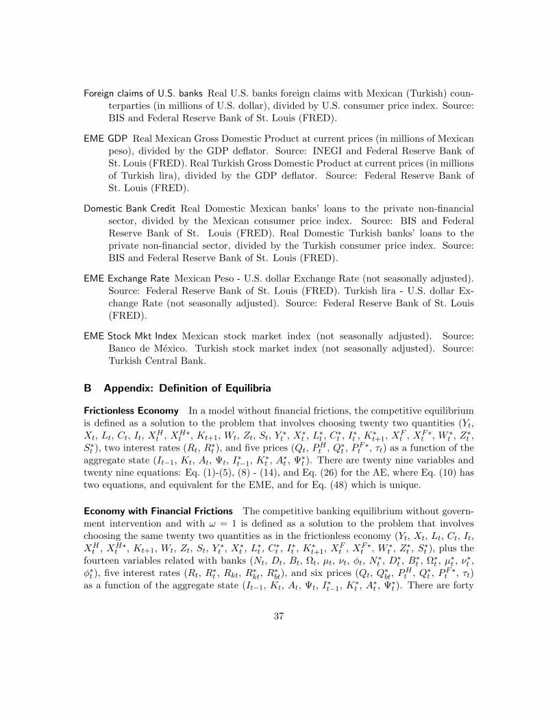
Foreign claims of U.S. banks Real U.S. banks foreign claims with Mexican (Turkish) coun-terparties (in millions of U.S. dollar), divided by U.S. consumer price index. Source:BIS and Federal Reserve Bank of St. Louis (FRED).

EME GDP Real Mexican Gross Domestic Product at current prices (in millions of Mexicanpeso), divided by the GDP deflator. Source: INEGI and Federal Reserve Bank ofSt. Louis (FRED). Real Turkish Gross Domestic Product at current prices (in millionsof Turkish lira), divided by the GDP deflator. Source: Federal Reserve Bank ofSt. Louis (FRED).

Domestic Bank Credit Real Domestic Mexican banks’ loans to the private non-financialsector, divided by the Mexican consumer price index. Source: BIS and FederalReserve Bank of St. Louis (FRED). Real Domestic Turkish banks’ loans to theprivate non-financial sector, divided by the Turkish consumer price index. Source:BIS and Federal Reserve Bank of St. Louis (FRED).

EME Exchange Rate Mexican Peso - U.S. dollar Exchange Rate (not seasonally adjusted).Source: Federal Reserve Bank of St. Louis (FRED). Turkish lira - U.S. dollar Ex-change Rate (not seasonally adjusted). Source: Federal Reserve Bank of St. Louis(FRED).

EME Stock Mkt Index Mexican stock market index (not seasonally adjusted). Source:Banco de Mexico. Turkish stock market index (not seasonally adjusted). Source:Turkish Central Bank.

B Appendix: Definition of Equilibria

Frictionless Economy In a model without financial frictions, the competitive equilibriumis defined as a solution to the problem that involves choosing twenty two quantities (Yt,Xt, Lt, Ct, It, X

Ht , XH∗

t , Kt+1, Wt, Zt, St, Y∗t , X∗t , L∗t , C

∗t , I∗t , K∗t+1, XF

t , XF∗t , W ∗t , Z∗t ,

S∗t ), two interest rates (Rt, R∗t ), and five prices (Qt, P

Ht , Q∗t , P

F∗t , τt) as a function of the

aggregate state (It−1, Kt, At, Ψt, I∗t−1, K∗t , A∗t , Ψ∗t ). There are twenty nine variables and

twenty nine equations: Eq. (1)-(5), (8) - (14), and Eq. (26) for the AE, where Eq. (10) hastwo equations, and equivalent for the EME, and for Eq. (48) which is unique.

Economy with Financial Frictions The competitive banking equilibrium without govern-ment intervention and with ω = 1 is defined as a solution to the problem that involveschoosing the same twenty two quantities as in the frictionless economy (Yt, Xt, Lt, Ct, It,XHt , XH∗

t , Kt+1, Wt, Zt, St, Y∗t , X∗t , L∗t , C

∗t , I∗t , K∗t+1, XF

t , XF∗t , W ∗t , Z∗t , S∗t ), plus the

fourteen variables related with banks (Nt, Dt, Bt, Ωt, µt, νt, φt, N∗t , D∗t , B

∗t , Ω∗t , µ

∗t , ν

∗t ,

φ∗t ), five interest rates (Rt, R∗t , Rkt, R

∗kt, R

∗bt), and six prices (Qt, Q

∗bt, P

Ht , Q∗t , P

F∗t , τt)

as a function of the aggregate state (It−1, Kt, At, Ψt, I∗t−1, K∗t , A∗t , Ψ∗t ). There are forty

37

seven variables and forty seven equations. Eq. (1)-(5), (8)-(14), for the AE, where Eq. (10)has two equations, and equivalent for the EME. Eq. (21), (23)-(26), (37)-(39) and similarfor the EME; and Eq. (30), (36), (43), (49), and (50).

C Appendix: EME Banks’ Optimization Problem

Let V ∗t (s∗t , b∗t , d∗t ) be the maximized value of V ∗t , given an asset and liability configuration

at the end of period t. The following incentive constraint must hold for each individualbank to ensure that a bank does not divert funds,

V ∗t (s∗t , b∗t , d∗t ) ≥ θ∗(Q∗t s∗t − ωQ∗btb∗t ), (C.1)

where the R.H.S. shows the funds that a bank can run away with, which are total value ofassets minus the borrowing from AE banks.

At the end of period t−1, the value of the bank satisfies the following Bellman equation

V ∗t (s∗t−1, b∗t−1, d

∗t−1) = Et−1Λ∗t−1,t

(1− σ∗)n∗t + σ∗

[maxs∗t ,b∗t ,d∗t

V ∗(s∗t , b∗t , d∗t )

]. (C.2)

The problem of the bank is to maximize Equation (C.2) subject to the borrowing constraint,Equation (C.1).

We guess and verify that the form of the value function of the Bellman equation islinear in assets and liabilities,

V (s∗t , b∗t , d∗t ) = ν∗sts

∗t − ν∗btb∗t − ν∗t d∗t , (C.3)

where ν∗st is the marginal value of assets at the end of period t, ν∗bt, the marginal cost ofholding foreign debt, and ν∗t , the marginal cost of deposits.

Maximizing the objective function (C.2) with respect to (C.1), with λ∗t as the constraintmultiplier, yields similar first-order conditions to the ones from the AE; those are

s∗t : ν∗st − λ∗t (ν∗st − θ∗Q∗t ) = 0

b∗t : ν∗bt − λ∗t (ν∗bt − θ∗ωQ∗bt) = 0

d∗t : ν∗t − λ∗t ν∗t = 0

λ∗t : θ∗ (Q∗t s∗t − ωQ∗btbt)− (ν∗sts

∗t − ν∗btb∗t − ν∗t d∗t ) = 0.

Rearranging terms yields:(ν∗btQ∗bt− ν∗t

)(1 + λ∗t ) = λ∗t θ

∗ω (C.4)(ν∗stQ∗t−ν∗btQ∗bt

)(1 + λ∗t ) = λ∗t θ

∗(1− ω) (C.5)[θ∗ −

(ν∗stQ∗t− ν∗t

)]Q∗t s

∗t −

[θ∗ω −

(ν∗btQ∗bt− ν∗t

)]Q∗btb

∗t = ν∗t n

∗t . (C.6)

38

Combining Equation (C.4) with Equation (C.5) results in(ν∗btQ∗bt− ν∗t

)1

ω=

(ν∗stQ∗t−ν∗btQ∗bt

)1

1− ω

µ∗bt = (µ∗t − µ∗bt)ω

1− ωµ∗bt = µ∗tω, (C.7)

where from the first to the second step we am using the definition of µ∗bt and µ∗t given inthe text in Equations (33) and (34), respectively.

Rewriting Equation (C.6) and defining φ∗t =θ∗−µ∗tν∗t

and φ∗bt =θ∗ω−µ∗bt

ν∗tyields

n∗t =1

φ∗tQ∗t s

∗t −

1

φ∗btQ∗btb

∗t . (C.8)

Now expressing the guess of the value function, Equation (C.3), in terms of the networth and international debt,

V (s∗t , b∗t , d∗t ) =

ν∗stQ∗t

Q∗t s∗t −

ν∗btQ∗bt

Q∗btb∗t − ν∗t d∗t

= (φ∗tµ∗t + ν∗t )n∗t +

(φ∗tµ

∗t

φ∗bt− µ∗bt

)Q∗btb

∗t . (C.9)

With this information I can verify the value function that corresponds to Equations (32),(33), and (34).

39

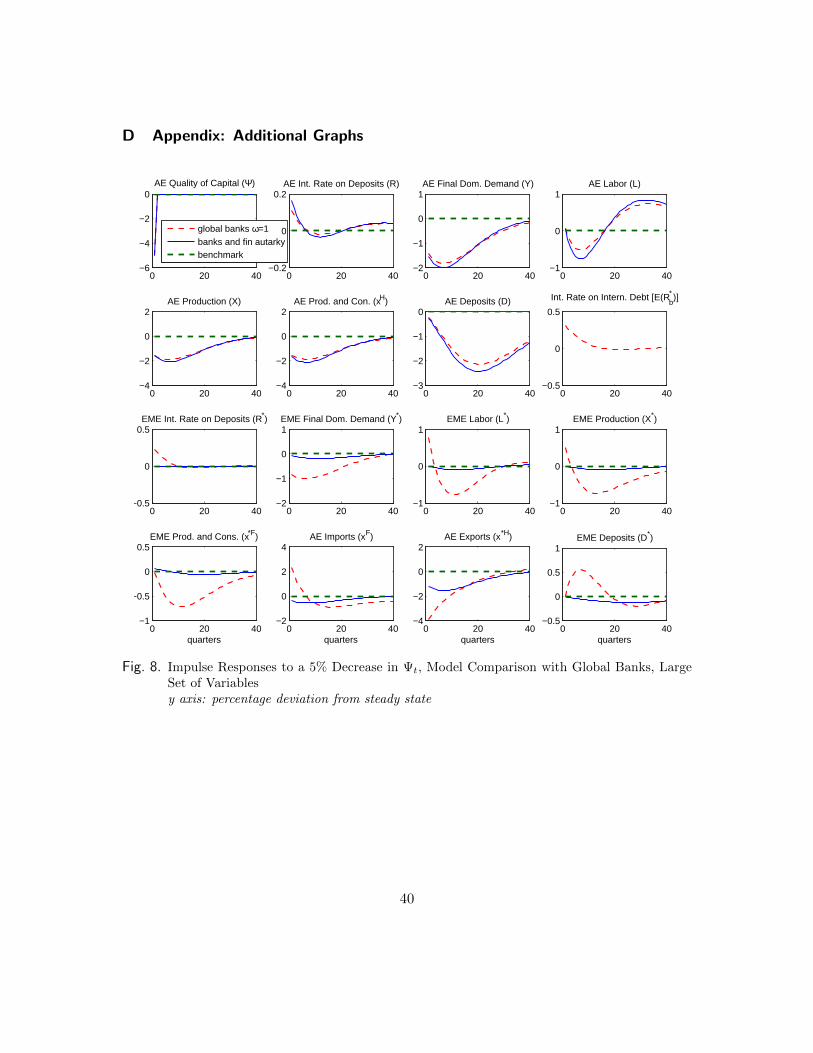
D Appendix: Additional Graphs

0 20 40−6

−4

−2

0AE Quality of Capital (Ψ)

0 20 40−0.5

0

0.5EME Int. Rate on Deposits (R*)

0 20 40−2

−1

0

1EME Final Dom. Demand (Y*)

0 20 40−1

0

1EME Labor (L*)

0 20 40−0.5

0

0.5

Int. Rate on Intern. Debt [E(Rb* )]

0 20 40−1

0

1EME Production (X*)

0 20 40−1

−0.5

0

0.5EME Prod. and Cons. (x*F)

quarters0 20 40

−0.5

0

0.5

1EME Deposits (D*)

quarters

global banks ω=1banks and fin autarkybenchmark

0 20 40−0.2

0

0.2AE Int. Rate on Deposits (R)

0 20 40−2

−1

0

1AE Final Dom. Demand (Y)

0 20 40−1

0

1AE Labor (L)

0 20 40−4

−2

0

2AE Production (X)

0 20 40−4

−2

0

2AE Prod. and Con. (xH)

0 20 40−2

0

2

4AE Imports (xF)

quarters0 20 40

−4

−2

0

2AE Exports (x*H)

quarters

0 20 40−3

−2

−1

0AE Deposits (D)

Fig. 8. Impulse Responses to a 5% Decrease in Ψt, Model Comparison with Global Banks, LargeSet of Variablesy axis: percentage deviation from steady state

40

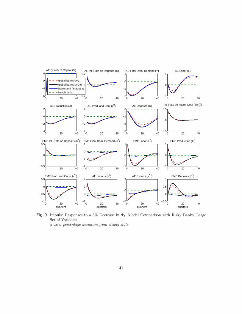
0 20 40−6

−4

−2

0AE Quality of Capital (Ψ)

global banks ω=1

global banks ω=0.6banks and fin autarkybenchmark

0 20 40−0.5

0

0.5EME Int. Rate on Deposits (R*)

0 20 40−2

−1

0

1EME Final Dom. Demand (Y*)

0 20 40−1

0

1EME Labor (L*)

0 20 40−0.5

0

0.5

Int. Rate on Intern. Debt [E(Rb* )]

0 20 40−1

0

1EME Production (X*)

0 20 40−1

−0.5

0

0.5EME Prod. and Cons. (x*F)

quarters0 20 40

−0.5

0

0.5

1EME Deposits (D*)

quarters

0 20 40−0.2

0

0.2AE Int. Rate on Deposits (R)

0 20 40−2

−1

0

1AE Final Dom. Demand (Y)

0 20 40−1

0

1AE Labor (L)

0 20 40−4

−2

0

2AE Production (X)

0 20 40−4

−2

0

2AE Prod. and Con. (xH)

0 20 40−2

0

2

4AE Imports (xF)

quarters0 20 40

−5

0

5AE Exports (x*H)

quarters

0 20 40−3

−2

−1

0AE Deposits (D)

Fig. 9. Impulse Responses to a 5% Decrease in Ψt, Model Comparison with Risky Banks, LargeSet of Variablesy axis: percentage deviation from steady state

41

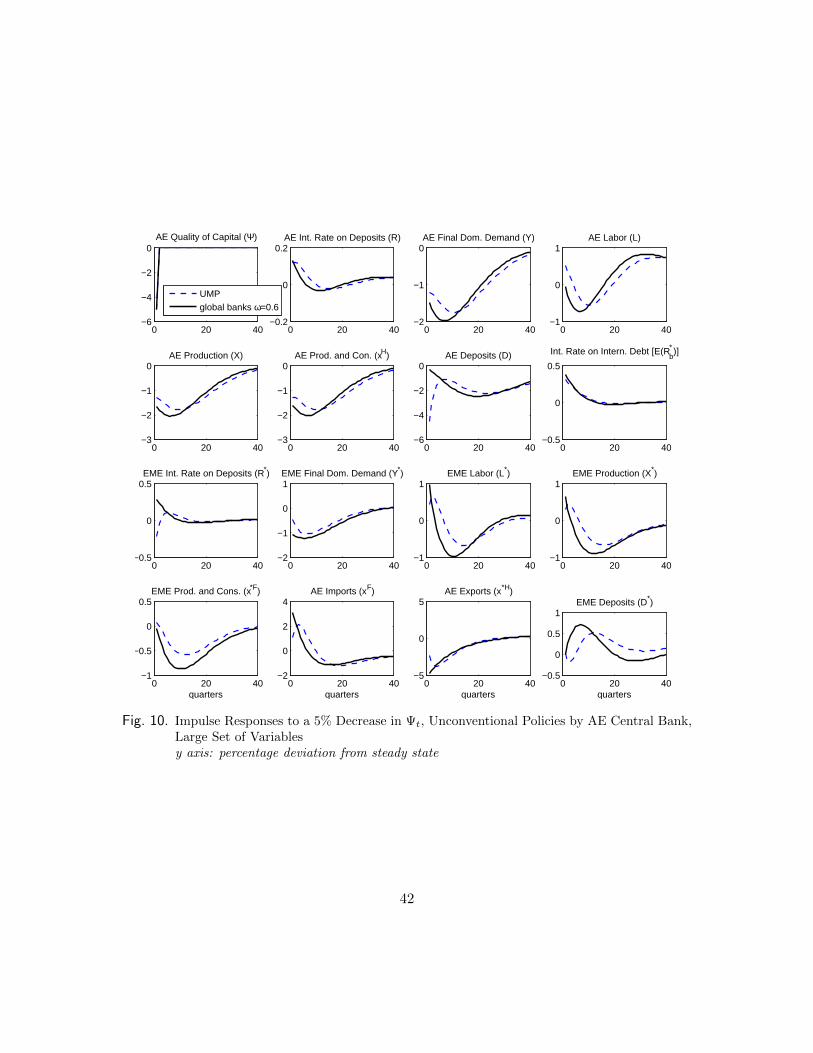
0 20 40−6

−4

−2

0AE Quality of Capital (Ψ)

0 20 40−0.5

0

0.5EME Int. Rate on Deposits (R*)

0 20 40−2

−1

0

1EME Final Dom. Demand (Y*)

0 20 40−1

0

1EME Labor (L*)

0 20 40−0.5

0

0.5

Int. Rate on Intern. Debt [E(Rb* )]

0 20 40−1

0

1EME Production (X*)

0 20 40−1

−0.5

0

0.5EME Prod. and Cons. (x*F)

quarters0 20 40

−0.5

0

0.5

1EME Deposits (D*)

quarters

UMP

global banks ω=0.6

0 20 40−0.2

0

0.2AE Int. Rate on Deposits (R)

0 20 40−2

−1

0AE Final Dom. Demand (Y)

0 20 40−1

0

1AE Labor (L)

0 20 40−3

−2

−1

0AE Production (X)

0 20 40−3

−2

−1

0AE Prod. and Con. (xH)

0 20 40−2

0

2

4AE Imports (xF)

quarters0 20 40

−5

0

5AE Exports (x*H)

quarters

0 20 40−6

−4

−2

0AE Deposits (D)

Fig. 10. Impulse Responses to a 5% Decrease in Ψt, Unconventional Policies by AE Central Bank,Large Set of Variablesy axis: percentage deviation from steady state

42

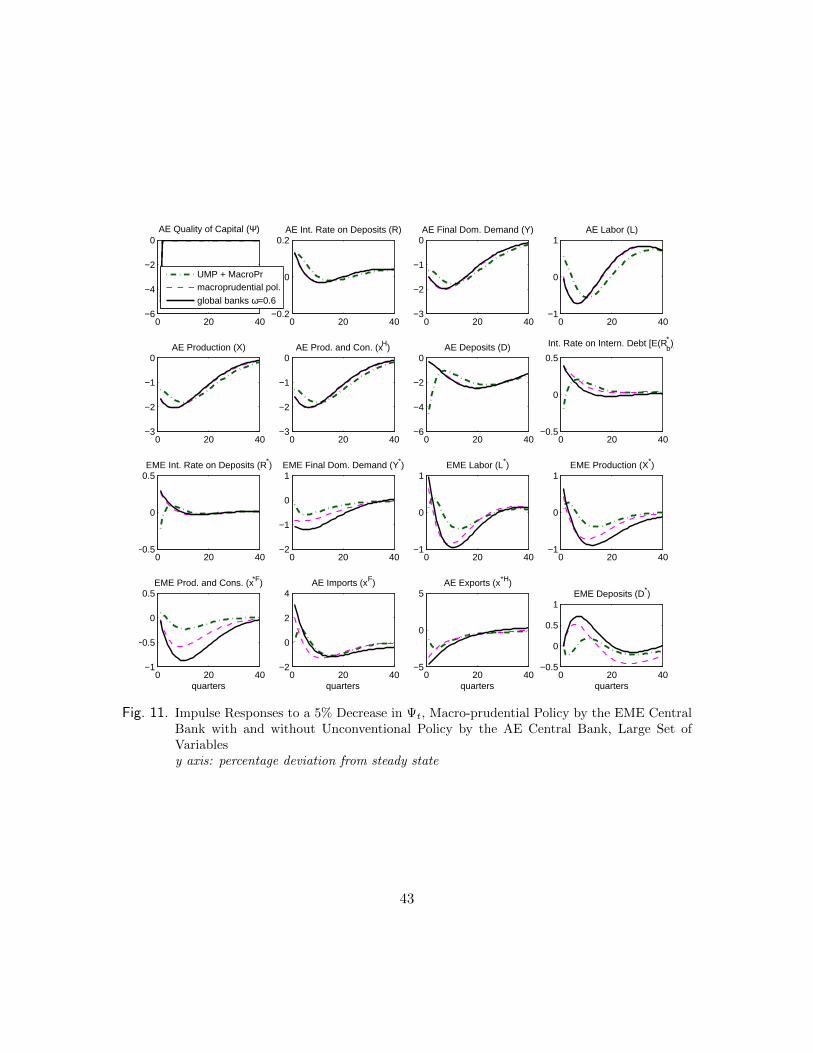
0 20 40−6

−4

−2

0AE Quality of Capital (Ψ)

0 20 40−0.5

0

0.5EME Int. Rate on Deposits (R*)

0 20 40−2

−1

0

1EME Final Dom. Demand (Y*)

0 20 40−1

0

1EME Labor (L*)

0 20 40−0.5

0

0.5

Int. Rate on Intern. Debt [E(Rb* )]

0 20 40−1

0

1EME Production (X*)

0 20 40−1

−0.5

0

0.5EME Prod. and Cons. (x*F)

quarters0 20 40

−0.5

0

0.5

1EME Deposits (D*)

quarters

UMP + MacroPrmacroprudential pol.

global banks ω=0.6

0 20 40−0.2

0

0.2AE Int. Rate on Deposits (R)

0 20 40−3

−2

−1

0AE Final Dom. Demand (Y)

0 20 40−1

0

1AE Labor (L)

0 20 40−3

−2

−1

0AE Production (X)

0 20 40−3

−2

−1

0AE Prod. and Con. (xH)

0 20 40−2

0

2

4AE Imports (xF)

quarters0 20 40

−5

0

5AE Exports (x*H)

quarters

0 20 40−6

−4

−2

0AE Deposits (D)

Fig. 11. Impulse Responses to a 5% Decrease in Ψt, Macro-prudential Policy by the EME CentralBank with and without Unconventional Policy by the AE Central Bank, Large Set ofVariablesy axis: percentage deviation from steady state

43