robust analysis of the basic economic order quantity …
TRANSCRIPT

The Pennsylvania State University
The Graduate School
College of Engineering
ROBUST ANALYSIS OF THE BASIC ECONOMIC ORDER QUANTITY MODEL
AND DETERMINISTIC SERIAL TWO-ECHELON INVENTORY MODEL
A Thesis in
Industrial Engineering
by
Sang Jin Kweon
2013 Sang Jin Kweon
Submitted in Partial Fulfillment
of the Requirements
for the Degree of
Master of Science
December 2013

The thesis of Sang Jin Kweon was reviewed and approved* by the following:
José A. Ventura
Professor of Industrial and Manufacturing Engineering
Thesis Advisor
Chia-Jung Chang
Assistant Professor of Industrial and Manufacturing Engineering
Paul Griffin
Professor of Industrial and Manufacturing Engineering
Peter and Angela Dal Pezzo Department Head Chair
*Signatures are on file in the Graduate School

iii
ABSTRACT
Since holding an inventory has its advantages and disadvantages, inventory is often
referred to as “a double-edged sword.” Thus, managing inventory wisely is one of the critical
success factors in business. A variety of research has investigated the systematic management of
inventory. General research has assumed that all parameters are either known and deterministic or
uncertain, but their values are all governed by probability distributions. Unfortunately, the
parameters are ordinarily unknown, and furthermore, it is also hard to identify their probability
information. This thesis assumes that all parameters are unknown and information about their
probability distributions is also unknown. In this uncertain situation, a robust optimization point
of view describes each unknown parameter as a continuous value that is restricted to some
prespecified interval. To address uncertain data input, this thesis uses robust optimization to
analyze the basic Economic Order Quality (EQQ) model and the deterministic serial two-echelon
inventory model.
First of all, this thesis derives the functions that show the upper and lower bounds of
EOQs under input data uncertainty. By considering the functions together, this thesis develops the
closed form expressions that characterize the set of all possible EOQs and corresponding
minimum average costs. Because this set predicts all possible inventory situations given unknown
parameters, it demonstrates variability of the basic EOQ model’s minimum average cost.
Also, this thesis analyzes the effect of randomness in the worst case scenario, and
suggests the optimal order policy of the basic EOQ model to minimize the worst error. This thesis
considers two minimax analyses – the ratio approach and the difference approach. These analyses
prove that the geometric mean or the arithmetic mean of the maximum and the minimum EOQ’s
provides the optimal order policy that produces the smallest possible error in the worst case.
iv
Finally, this thesis extends the closed form expressions of the basic EOQ model to the
deterministic serial two-echelon inventory model for robust analysis. The deterministic serial
two-echelon inventory model has a multiplicity factor for the order quantity. Thus, this thesis first
develops the closed form expressions that describe the set of all possible optimal order quantities
and corresponding minimum total costs for general multiplicity factor. This set is called
variability of the minimum total cost because this set predicts all possible inventory situation of
the deterministic serial two-echelon inventory model. But, the multiplicity factor can actually take
different positive integer values under input data uncertainty. Thus, after calculating all possible
candidates of the optimal multiplicity factor, we apply our closed form expressions to draw
variability for each candidate then we compare their variability. One interesting observation is
that the area of variability decreases logarithmically as the multiplicity factor increases. It
indicates that an inventory manager can reduce variability by increasing the multiplicity factor
when making or renewing contract. But one problem is that sometimes upper bound of the
minimum total cost also increases as the multiplicity factor increases. To avoid this problem, we
suggest a method to find the best multiplicity factor at which upper bound of the minimum total
cost is minimized with small variability.

v
TABLE OF CONTENTS
List of Figures ......................................................................................................................... vii
List of Tables ........................................................................................................................... ix
Acknowledgements .................................................................................................................. x
Chapter 1 INTRODUCTION ................................................................................................... 1
1.1 Necessity of Inventory Management ......................................................................... 1
1.2 Motivation .................................................................................................................. 2
1.3 Research Direction ..................................................................................................... 3
Chapter 2 LITERATURE REVIEW ........................................................................................ 6
2.1 Robust Single-Echelon Inventory Problems .............................................................. 6
2.2 Stochastic Single-Echelon Inventory Problems ......................................................... 8
2.3 Stochastic Multi-Echelon Inventory Problems .......................................................... 9
2.4 Distinction between Our Thesis and Previous Studies ............................................... 11
Chapter 3 BACKGROUND ..................................................................................................... 13
3.1 The Basic Economic Order Quantity (EOQ) Model .................................................. 13
3.2 Minimax Analysis ...................................................................................................... 16
3.3 The Deterministic Serial Two-Echelon Inventory Model for Supply Chain
Management ............................................................................................................. 16
Chapter 4 ROBUST ANALYSIS ............................................................................................ 22
4.1 Robust Analysis of the Basic EOQ Model ................................................................. 24
4.2 Minimax Analysis of the Basic EOQ Model ............................................................. 32
4.2.1 The ratio approach to minimize the worst error .............................................. 32
4.2.2 The difference approach to minimize the worst error ..................................... 38
4.3 Robust Analysis of the Deterministic Serial Two-Echelon Inventory Model ............ 44

vi
4.3.1 When the multiplicity factor is fixed ............................................................... 47
4.3.2 When the multiplicity factor is not fixed ......................................................... 58
Chapter 5 NUMERICAL EXAMPLES ................................................................................... 60
5.1 A Numerical Example for Robust Analysis of the Basic EOQ Model ...................... 60
5.2 A Numerical Example for Minimax Analysis of the Basic EOQ Model ................... 64
5.3 A Numerical Example for Robust Analysis of the Deterministic Serial Two-
Echelon Inventory Model ......................................................................................... 68
Chapter 6 CONCLUSION ....................................................................................................... 79
6.1 Summary of the Thesis............................................................................................... 79
6.2 Contribution ............................................................................................................... 83
6.3 Future Research .......................................................................................................... 83
REFERENCES ........................................................................................................................ 84

vii
LIST OF FIGURES
Figure 1. Serial two-echelon inventory system ........................................................................ 17
Figure 2. Synchronized inventory levels at the two installations for ...................... 18
Figure 3. Upper bound of the set of the minimum average costs ............................................ 27
Figure 4. Lower bound of the set of the minimum average costs ............................................ 29
Figure 5. Feasible optimal region of the basic EOQ model ..................................................... 30
Figure 6. Effect of randomness in the worst error ratio ........................................................... 38
Figure 7. Effect of randomness in the worst error difference .................................................. 43
Figure 8. Upper bound of the set of the minimum total costs .................................................. 51
Figure 9. Lower bound of the set of the minimum total costs ................................................. 53
Figure 10. Two-dimensional feasible optimal region of the deterministic serial two-
echelon inventory model ......................................................................................... 54
Figure 11. Three-dimensional feasible optimal region of the deterministic serial two-
echelon inventory model ......................................................................................... 56
Figure 12. Logarithmically decreasing relationship between the interval of the optimal
order quantity at installation 2 and the multiplicity factor ...................................... 57
Figure 13. Four expressions to describe the feasible optimal region of the basic EOQ
model ...................................................................................................................... 62
Figure 14. Four examples that shows effect of intervals to the feasible optimal region .......... 63
Figure 15. Worst error ratio function ....................................................................................... 66
Figure 16. Worst error difference function .............................................................................. 67

viii
Figure 17. Four expressions to characterize the two-dimensional feasible optimal region
of the deterministic serial two-echelon inventory model ........................................ 70
Figure 18. Extension of the two-dimensional feasible optimal region to the three-
dimensional feasible optimal region ....................................................................... 72
Figure 19. Logarithmically decreasing relationship between the multiplicity factor and
the area of the feasible optimal region .................................................................... 74
Figure 20. Twelve different two-dimensional feasible optimal regions of the deterministic
serial two-echelon system according to the multiplicity factor .............................. 77
Figure 21. Change of the upper and lower bounds of the minimum total cost of the
deterministic serial two-echelon inventory model .................................................. 78
ix
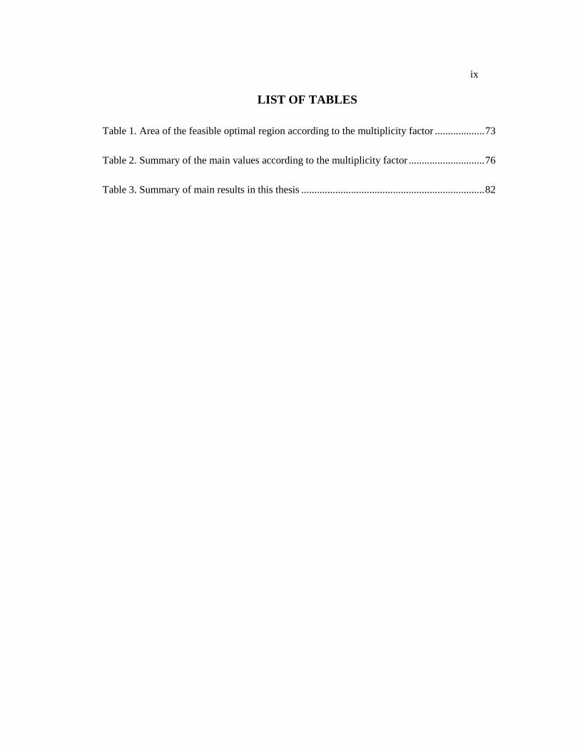
LIST OF TABLES
Table 1. Area of the feasible optimal region according to the multiplicity factor ................... 73
Table 2. Summary of the main values according to the multiplicity factor ............................. 76
Table 3. Summary of main results in this thesis ...................................................................... 82
x
ACKNOWLEDGEMENTS
It is my honor to thank all those who made this thesis clear and specific. Above all, I
would like to show my gratitude to my academic adviser, Dr. Ventura. I am wholeheartedly
indebted to him for all the guidance and inspiration he has provided for me over the years. He
first suggested the idea about robust analysis of the basic economy order quantity model, and he
encouraged me to find solutions with his valuable comments whenever I faced difficulties. He is
my role model not only as an academic adviser but also as a great life mentor.
In addition, I would like to thank Dr. Chang that she was willing to review my thesis with
her valuable advice. I took her class, IE 522 (Discrete Event Systems Simulation), in Fall 2012
semester, and it was my great opportunity to build intuition about randomness of the parameters.
Last but not the least, I am grateful for my parents’ eternal love and infinite support. They
have often gone hungry themselves in Seoul, South Korea, so that I have had enough to eat here
in University Park, PA, U.S.A. If my parents did not aid me both materially and spiritually, I
would not be here writing my thesis acknowledgements. I will never forget my parents’ love for
me forever.

1
Chapter 1
INTRODUCTION
1.1 Necessity of Inventory Management
In 2012, Walmart spent 40.714 billion dollars to manage inventory (Walmart 2013). This
amount accounts for about 10% of the net sales, and Walmart plans to increase their investment
on inventory consistently. Certain investment on inventory is necessary for a company to survive
as there are two basic reasons for holding an inventory. First, inventories play a role as buffers
when supply fails to meet demand. Second, a large purchase of inventories leads to economies of
scale. If someone orders one unit whenever he needs an item, it will cost a lot. But if he orders an
item in bulk, he can obtain quantity discounts. These advantages attract a company to hold an
inventory. However, keeping an inventory is not always good. The more inventory we have, the
more inventory holding cost we have. Besides, some overstocks can become perishable or old-
fashioned while they are being kept in the warehouse. According to an article published in
Bartner News, manufacturers, wholesalers, direct marketers, and retailers spent a total of 350
billion dollars on handling their surplus inventory and overstock in 1999 (Tuesday Barter Report
2000). These advantages and disadvantages imply that inventory could end up being “a double-
edged sword.” Thus, managing inventory wisely is one of the critical success factors in business.
As the market and the supply chain of a corporation become more complicated and
global, inventory management needs to be prompter in dealing with the changes of the business.
For example, Amazon, one of the world’s largest online retailers, sold 27 million items on Cyber
Monday, November 26, 2012 (Yarow 2012). It would be impossible to meet the high demand of
various items if Amazon did not have established a well-prepared inventory strategy. Forbes has

2
projected that this market regarding e-commerce will grow by an annual average of 11 percent
each year by 2017 (O’connor 2013). This environment will require a worldwide, robust inventory
management strategy to deal with huge demands for diverse items all around the world.
1.2 Motivation
Several studies have been performed to manage inventory systematically. Harris (1913) is
well-known to be the first who suggested the Economic Order Quantity (EOQ) model to manage
inventory mathematically. Although the EOQ model is often used in practice, it has two main
weak points. The first point is that the real world supply chain is more complicated than his
inventory model, and the second one is that the assumption about input data for the EOQ model
that “demand per unit time (D), ordering cost (K), and inventory holding cost per unit per unit
time (h) are known” are unrealistic in real life inventory problem because input data may be
unknown or change frequently (Gallego et al. 2001).
To make up for these weak points, numerous applications have been studied steadily (Yu
1997). As one of the applications to make up for input data uncertainty, Lowe and Schwarz
(1983), Dobson (1988), and Schwarz (2008) relaxed the assumption that input data are known.
Instead, they assumed that the parameters, such as D, K, and h, are restricted to some prespecified
intervals, and measured how much total cost changes as these parameters change in their
intervals, which is called sensitivity analysis of the EOQ model. Furthermore, they applied the
sensitivity analysis of inventory cost rate to errors to the two minimax criteria – the first one is
using the difference between the feasible average cost rate the company faces, , and the
minimum average cost rate the company would face if there were no error in estimation,
, and the second one is the ratio of to – in order to suggest the
method that can avoid the worst possible outcome.
3
This thesis is motivated by their work about the sensitivity analysis and the minimax
criteria, given that all the parameters are unknown over known intervals. Since we do not have
any information about exact values or probabilities of the parameter, this problem is called input
data uncertain situation, and be categorized as an robust optimization problem (Rosenhead et al.
1972). Thus in this thesis we will approach the EOQ model from a robust optimization point of
view, and search all the possible optimal cost sets of the EOQ model when all the input data, such
as D, K, and h change over known intervals. We will call this work as robust analysis because we
will investigate all the possible results under input data uncertainty (Snyder 2006). Then we will
extend our robust analysis of the EOQ model to the multi-echelon inventory model.
1.3 Research Direction
Lowe and Schwarz (1983), Dobson (1988), and Schwarz (2008) recognized that the
parameters that compose the EOQ model, such as D, K, and h, are likely to be unknown in the
real world inventory management. To reflect realistic circumstances management, they measured
the impact of all the parameters on the management cost when their values are uncertain, but
known only within some prespecified intervals. Their work is called sensitivity analysis of the
EOQ model since they analyzed how much the management cost is sensitive to each of these
parameters. On the other hand, it can be said that they built intuition about the robustness of EOQ
because their work is based on input data uncertain situation (Snyder 2006). This thesis is
influenced by their intuition about the robustness of EOQ. Thus, we start our study by
approaching their work about sensitivity analysis of the EOQ model from a robust optimization
point of view.
In this thesis, we mainly focus on the EOQ model and the deterministic serial two-
echelon inventory model. Our goal is to develop expressions to characterize the set of all possible

4
order quantities and corresponding average costs in closed form, and find the method to reduce
randomness of the worst error for the basic EOQ model and the deterministic serial two-echelon
inventory model when neither any information about exact values nor probabilities of all the
parameters is known. Thus, all the input data of the EOQ model and the deterministic serial two-
echelon inventory model are assumed to be unknown over prespecified intervals in this thesis.
To achieve the goal, this thesis consists of three main studies. First of all, we consider all
the combinations of the EOQ parameters when their values change in their continuous intervals.
The interval of EOQ is obtained by checking all the combinations. Separate combinations of the
parameters sometimes can lead to the same EOQ value with different minimum average costs,
meaning that each EOQ value can have the upper and lower bounds of the minimum average cost.
Thus, we develop expressions which characterize the upper and lower bounds of the minimum
average cost for each EOQ in closed form, respectively. By considering these two closed form
expressions together, we derive the set of all possible EOQ’s and corresponding minimum
average costs while all the EOQ parameters are changing over prespecified intervals.
Secondly, this thesis finds out the robust order policy of the EOQ model to minimize the
worst error. Since all the input data are generally unknown in the real world, these values are
sometimes estimated. But estimation of the input value often includes errors, and wrong
estimation can result in ascending cost. Thus, it is significant to measure the impact of error on
the cost and minimize the worst error from a robust optimization point of view. Lowe and
Schwarz (1983) introduced two minimax criteria – the difference approach and the ratio approach
– to find the worst error, and discussed how to minimize the worst error. This thesis similarly
follows these two minimax analyses. But we also analyze the effect of randomness in the worst
case for all EOQs, and develop the closed form optimal order policy to produce the smallest error
in the worst case.

5
Lastly, this thesis extends our closed form expressions for the basic EOQ model which
characterize the set of all possible EOQ’s and corresponding minimum average costs to the
deterministic serial two-echelon inventory model. Since it is a two-echelon system, we first
consider the multiplicity factor for the order quantity. However, the multiplicity factor can take
different positive integers when all the parameters are uncertain over known intervals. This
complicates the problem. Thus, we first regard the multiplicity factor as fixed. Then, we derive
expressions to characterize the set of all possible optimal order quantities and corresponding
minimum total in closed form costs for the fixed multiplicity factor. Next, we calculate all the
possible candidates of the multiplicity factor. Then, we apply our closed form expressions to each
multiplicity factor. This analysis helps us find the best multiplicity factor to minimize upper
bound of the minimum total cost of the two-echelon inventory model with reducing the effect of
randomness.
The body of this thesis is organized as follows. In Chapter 2, we summarize the literature
review about inventory models, especially about EOQ models and multi-echelon inventory
models. In Chapter 3, we briefly review the concepts about the basic EOQ model (Section 3.1),
minimax analysis (Section 3.2), and deterministic serial two-echelon inventory model (Section
3.3). Then in Chapter 4, we do robust analysis (Section 4.1), analyze the effect of randomness in
the worst case and make it minimize (Section 4.2) of the basic EOQ model. Then we extend our
robust analysis of the basic EOQ model to the deterministic serial two-echelon inventory model
(Section 4.3). In Chapter 5, numerical examples that give shape to Chapter 4 are discussed.
Finally in Chapter 6, we provide conclusions and suggest future research topics.

6
Chapter 2
LITERATURE REVIEW
As the classic inventory models reach the limit on reflecting the competitive industrial
environment, a variety of research has been published to overcome the limitations. In particular,
some of inventory studies have been developed under uncertain parameters. Rosenhead et al.
(1972) classified uncertain parameters into two categories: (i) robust optimization problem, and
(ii) stochastic optimization problem. The stochastic optimization problem assumes that
parameters are uncertain, but their values follow some known probability distributions. On the
other hand, the robust optimization problem assumes that parameters are unknown, and
furthermore, any information about their probability distributions is also unknown. Instead,
continuous parameters are restricted to some prespecified intervals in case of the robust
optimization problem. Note that this thesis is based on the robust optimization problem. In this
chapter, we briefly introduce previous studies about single-echelon and multi-echelon inventory
model, both from a robust optimization point of view and a stochastic optimization point of view.
2.1 Robust Single-Echelon Inventory Problems
The first class focuses on the single-echelon inventory model, given that parameters are
restricted to some prespecified intervals without any information about their probability. To solve
this robust optimization problem, the first class has introduced sensitivity analysis or fuzziness.
Also, some of them used minimax analysis to optimize the worst case scenario of the inventory
system. When the demand is assumed to be non-stationary, Karlin (1960) found out the best
ordering policies for linear purchase cost and for convex purchase cost, and Morton (1978)
7
developed the bounds of the inventory level and its cost for infinite horizon inventory model.
Lowe and Schwarz (1983) did sensitivity analysis when the parameters of the basic EOQ model
belong to a closed interval. To measure the error rate in parameter estimation, Lowe and Schwarz
proposed the two measurements – the first measurement of error rate was using the difference
between an actual average cost and the minimum average cost, and the other one measured the
ratio of an actual average cost to the minimum average cost. Dobson (1988) extended the Lowe
and Schwarz’s work, and proved the insensitivity of the average cost of EOQ policy as the
parameters change under uncertainty. In his paper Dobson showed that the expected error ratio is
small and its bound is independent of common distributions. Yu (1997) considered the EOQ
model with parameters such as the annual demand rate, the ordering cost and the inventory
holding cost being unknown, and suggested a linear time algorithm to derive the robust decisions
under two robustness criteria – One minimizes the maximum total inventory costs, and the other
one minimizes the maximum percentage deviation from optimality. Then Yu showed the robust
decisions by a linear time algorithm has better performance than the stochastic optimization
decisions. Schwarz (2008) also extended Lowe and Schwarz’s work about error ratio, and
suggested the concept of penalty-cost ratio, which plays a role as a measurement of the sensitivity
analysis. On his paper, Schwarz showed how much the penalty-cost ratio changes when the
assumptions of the basic EOQ model are relaxed, and Schwarz did sensitivity analysis according
to the change of penalty-cost ratio. Ren (2010) used a simulation model to examine the robustness
of the basic EOQ model on the assumption that input data follow uniform or normal probability
distributions. Ouyang and Yao (2002) introduced two fuzziness of annual demand to a continuous
review mixed inventory model to reflect that various circumstances change the annual demand in
real life inventory problem, and developed an algorithm which suggests the optimal ordering
strategy when the lead time and the annual demand are assumed to be unknown. Sana (2011) also
focused on the sensitivity of price to a deteriorating product, and devised the finite horizon

8
deterministic EOQ model both for the rate of demand being a quadratic function and being a
negative power function of selling price, respectively. These models calculate the optimal order
quantity and optimal sales prices at which a manufacturer maximizes his profit. Then Sana did
sensitivity analysis how the parameters of the EOQ model affect the optimal strategy.
2.2 Stochastic Single-Echelon Inventory Problems
The second approach considers the single-echelon inventory model, on the assumption
that value of parameters is governed by known probability distribution. In particular, some of the
approach suggested the method to manage the market variability by applying minimax analysis or
distribution free model to the demand data. For a single-period newsvendor problem, Scarf
(1958) found the optimal stock level at which the minimum profit is maximized for all demand
distributions when only the mean and the standard deviation of the demand distribution are
assumed to be known. Gallego and Moon (1993) proved the Scarf’s optimal ordering rule for a
single-period newsvendor problem, and extended the results to the fixed ordering cost case, the
random yield case, and the multi-product case. Kasugai and Kasegai (1960) also extended Scarf’s
work to a multi-period newsvendor problem, and used dynamic programming to Scarf’s work for
the demand following uniform distribution. They also compared the results by minimax regret
ordering policy to the result of the minimax policy (Kasugai and Kasegai 1961). As one of the
further applications of Scarf’s work, Moon and Gallego (1994) used minmax distribution free
procedure to minimize the worst distribution for each decision variable, and applied it both to
continuous review inventory model and the periodic review inventory model with lost sales and
backorders in which only the mean and the standard deviation of the demand are assumed to be
known. Moon and Choi (1997) followed up Moon and Gallego’s procedures, and applied
distribution free procedure to the composite models in order to find the optimal order quantity.

9
Gallego (1998) used minimax analysis to devise a closed form distribution free solution for
continuous review inventory model when backorder cost is time-weighted. Then Gallego also
showed the robustness of distribution free, batch size heuristics against demand variability. Lin
(2008) applied the minimax distribution free approach to minimize a total cost for the continuous
review inventory model with backorder price discount in case of lead time being interdependent
on decrease of ordering cost. Gallego et al. (2001) assumed that demand is a discrete random
variable and it takes values in a known countable set. Then, they developed a formulation for the
linear programming problem of finding the optimal inventory policy to minimize the maximum
expected cost over all distributions that satisfy linear constraints. Main advantage of their model
is flexibility of the model. In other words, their model can include various linear constraints on
the demand distribution whereas the previous studies which assumed that the demand mean and
standard deviation are known cannot easily combine additional constraints.
2.3 Stochastic Multi-Echelon Inventory Problems
As industrial cooperation becomes more emphasized and supply chain becomes more
global, the studies on single-echelon inventory system have been extended to multi-echelon
inventory system by applying stochastic models. Clark and Scarf (1960) are well-known to be the
first who developed the optimal ordering policy of the two-echelon inventory system. Sherbrooke
(1968) studied the optimality of two-echelon system in which backorders are allowed at retailers.
Federgruen and Zipkin (1984) used a dynamic programming to generalize Clark and Scarf’s work
and to approximate the minimum expected cost of the two-echelon inventory system. Rosling
(1989) applied Clark and Scarf’s work to assembly systems, and derived the optimal reorder
policies under demand uncertainty. Axsäter and Zhang (1999) applied two-echelon model to the
system that consists of one central warehouse and several identical retailers, and analyzed the

10
joint replenishment policy in which the retailer with the lowest stock level makes a batch ordering
when the total sum of retailer stocks are becoming under the joint reorder point predetermined.
Hopp et al. (1999) estimated the Lagrange multipliers in the expressions that calculate the
inventory control parameters for the optimal inventory policy in a two-echelon system by using a
search algorithm. Erkip et al. (1990) studied the three-echelon inventory system which consist of
one supplier, one depot, and N-warehouses, where N is a positive integer for number of
warehouses, in which product demands are assumed to be correlated both across warehouses and
through time. Then Erkip et al. found out the optimal ordering quantity as a function of the
correlation level through time. Since the previous multi-echelon approaches mentioned above
were limited to serial two- or three-echelon systems, various studies have been extended to
general multi-echelon systems. Langenhoff and Zijm (1990) did average cost analysis of the
stochastic two-echelon serial system, and extended it to an N-echelon seiral system. Van der
Heijden et al. (1997) considered the general multi-echelon periodic review distribution systems,
and focused on investigating stock allocation policies in the system. Diks and de Kok (1998)
derived the optimal replenishment policy that minimizes the expected inventory holding cost and
penalty cost in a divergent multi-echelon periodic review inventory system. Morton and Pentico
(1995) and Anupindi et al. (1996) proposed myopic heuristics to the finite horizon non-stationary
stochastic inventory problem, and Iida (2001) applied the myopic heuristics to the multi-echelon
inventory problem with non-stationary demands in order to find the optimal multi-echelon
inventory policies. Rau et al. (2003) did sensitivity analyses of the total optimal solution on
demand and deterioration rate in a multi-echelon system for perishable goods. Yang and Lin
(2010) applied a serial multi-echelon system to a Just-In-Time model. Zhou et al. (2013) extended
a multi-echelon system to multi-product model, and solved it by Genetic Algorithm method. In
common with simulation-based methods to examine the robustness of the basic EOQ model (Ren
2010), simulation applications to the multi-echelon system have been actively discussed.
11
Glasserman and Tayur (1995) used simulation methods to do sensitivity analysis of costs on
demand distributions in multi-echelon systems. Tee and Rossetti (2002) also verified the
robustness of the multi-echelon continuous review inventory models discussed by Axsäter (2000)
by applying a simulation method. Tsai and Zheng (2013) derived the optimal order quantity at
which the total cost is minimized in the two-echelon system subject to service level constraints
with respect to the expected response time by using a simulation optimization framework.
2.4 Distinction between Our Thesis and Previous Studies
The previous studies considered various inventory systems with various situations, but
we were still wondering the robustness of the inventory models in closed form if we cannot have
sufficient information to estimate the probability distributions of the input data under dynamic
environments. Thus in this thesis we revisit the traditional EOQ model, and extend Lowe, Dobson,
and Schwarz’s works (Lowe and Schwarz 1983, Dobson 1988, Schwarz 2008). Then we derive
the robust analysis expressions in closed form when all the parameters of the basic EOQ model
are uncertain but we only have rough intervals of their input data obtained by experience. Our
thesis starts with a line of research similar to that of Lowe and Schwarz, but we characterize the
set of all possible EOQ’s and corresponding minimum average costs in closed form from a robust
optimization point of view, while Lowe and Schwarz focused on the set of the penalty-cost ratio
and sensitivity analysis. Also in this thesis, we extend Lowe and Schwarz’s work (1983) and
Dobson’s proof (1988), and consider two minimax analyses – the ratio approach and the
difference approach – to derive a closed-form optimal order policy that minimizes the worst error,
which is based on the set of all possible EOQ’s and corresponding minimum average costs. Then
we extend our robust analysis to the deterministic serial two-echelon inventory system. The
multi-echelon inventory model has the multiplicity factor for the order quantity, and the

12
multiplicity factor can take different positive integer values under input data uncertainty. Thus,
we suggest the method to find the best multiplicity factor among the candidates that minimize
upper bound of the minimum total cost with its small variability.

13
Chapter 3
BACKGROUND
In this chapter we briefly summarize the background of inventory management that forms
the foundation of robust analysis of the inventory management in Chapter 4. In Section 3.1, we
will introduce the basic economic order quantity model to derive the minimum average cost at the
economic order quantity, and in Section 3.2, the concept of minimax analysis will be simply
explained to investigate the effect of randomness in the worst case in the basic EOQ model and
find the optimal policy to minimize the worst error. In Section 3.3 we will review that how the
basic EOQ model concept is extended to the multi-echelon inventory model, especially the
deterministic serial two-echelon inventory model. Section 3.1 and Section 3.2 are to be the basis
to do robust analysis and to minimize the worst error for the basic EOQ model. Section 3.3 is to
be the basis to do robust analysis of the deterministic serial two-echelon inventory model in a
supply chain.
3.1 The Basic Economic Order Quantity (EOQ) Model
Inventory management has been developed to handle supply of components and products.
Someone would merely want to increase his/her inventory quantities to manage the unexpected
demand, but this strategy can also increase the total inventory holding cost inevitably, whereas if
others simply wanted to decrease the total inventory holding cost, it would make the total
ordering cost increased because number of orders should be increased to meet demand. Thus,
inventory management considers all of these factors to find a best strategy which makes it not
only to satisfy demand but also minimize the sum of the inventory holding cost and the total

14
ordering cost. The two prominent inventory management approaches are either based on
probabilistic inventory models or deterministic inventory models.
Compared with the probabilistic inventory models, the deterministic inventory models
assume that demand is predictable. Based on constant demand per unit time, denoted by D, we
can derive ordering cost over some fixed time from ordering cost and inventory-holding cost. The
order quantity that minimizes the ordering cost is called the Economic Order Quantity (EOQ),
and it is one of the classical deterministic inventory models (Harris 1913). To set up the EOQ
model, the following assumptions are held:
(1) The ordering cost, denoted by K, is known and constant.
(2) The inventory holding cost per unit per unit time, denoted by h, is known and
constant.
(3) The order lead time is considered as zero. That is, the order quantity is received
instantaneously.
Based on the above assumptions, the average cost per unit time for an order quantity (Q),
denoted by C(Q), is derived as
(1)
The first term represents the average ordering cost per unit time, which is the ordering cost
multiplied by the average number of orders per unit time. That is, every time we order the amount
of Q, the cost is K, and we know the demand per unit time is D, thus the total number of order per
unit time is
. Therefore, the total ordering cost is
in the first part. Also, the second term
shows the average inventory holding cost per unit time, which is the inventory holding cost per
unit per unit time multiplied by the average inventory. On expecting the average order quantity,
we assume that the order quantity follows the uniform distribution between 0 and Q, thus the
average order quantity is
and the inventory holding cost per unit per unit time is . Thus,

15
is the average inventory cost per unit time. The first term is the reciprocal function for Q. That is,
since the largest possible value of an order quantity ( ) decreases the average number of orders
per unit time, the average ordering cost per unit time can be minimized by . On the other hand,
the second term is a monotonically-increasing linear function for Q. Thus, the smallest possible
value of an order quantity ( ) minimizes the average inventory cost per unit time. In this respect,
a certain order quantity exists to minimize the total average cost. We call this order quantity as
the optimal order quantity,
As the first step to find , Equation (1) is differentiated with respect to Q as
(2)
and then, in order to find , Equation (2) is set to zero. Then, solving for Q yields
√
(3)
Since we are interested in the minimum average cost with respect to , we replace in Equation
(1) by the expression in Equation (3). Then the minimum average cost, , is derived as
(√
)
√
√
√
√
(4)
We apply Section 3.1 to Section 4.1 in order to derive the minimum average costs
according to for the basic EOQ model.

16
3.2 Minimax Analysis
Minimax analysis is a decision making rule to minimize the maximum loss scenario
(Sion 1958). Minimax analysis is often used in robust optimization area in order to minimize the
worst case scenario when the parameters are unknown without any information about probability
distributions (Dem’yanov and Malozemov 1990). To consider the minimax analysis to the thesis,
we define two parameters; one for making the worst loss case, and the other one for minimizing
the set consisting of possible worst loss cases (Grossinho and Tersian 2001). For example, is an
order quantity related to loss, and is the order quantity a decision maker can control to
minimize the loss. Then the functions and , which explain the costs according to and
, can be used for minimax analysis as follows.
{
} (5)
To derive a solution for Equation (5), we solve the maximum part first, and then we minimize it.
The solution suggests how many order quantity should be ordered to minimize its worst loss
scenario.
Section 3.2 is to be used in Section 4.2 when we look for optimal order quantities to
avoid the worst error through two minimax frameworks; minimizing the worst error ratio and
minimizing the worst error difference.
3.3 The Deterministic Serial Two-Echelon Inventory Model for Supply Chain
Management
A supply chain consists of multi-echelon network to procure raw materials, process them
into products, and transport the products to retailer or final customers through a distribution
system. For example in the supply chain, a manufacturer can store an inventory at processing

17
point (first echelon), then store the intermediate goods or the final products at warehouse (second
echelon), then carry them to various distribution centers (third echelon). Such a system is called
multi-echelon inventory system (Hillier and Lieberman 2010). A supply chain manager uses the
inventory in one echelon to replenish the inventory at the next echelon, thus the multi-echelon
inventory system is one of the main topics we care about to manage the inventories in a supply
chain. To survive the competitive market, one of the key objectives of a supply chain is to
minimize the total cost associated with multi-echelon inventory system, but the analysis of multi-
echelon inventory model is more complicated than the analysis of single facility inventory model
in Section 3.1. Thus in this thesis, we consider a simple multi-echelon inventory system, the
deterministic serial two-echelon system, to be analyzed.
Serial two-echelon system is composed of two installations, installation 1 for a
manufacturer and installation 2 for a distribution center. Figure 1 describes this system.
Figure 1. Serial two-echelon inventory system
To set up the serial two-echelon model, the following assumptions are held:
(1) The assumptions of the basic EOQ model held in Section 3.1 hold at installation 2,
where demand rate per unit time (D) is constant and is an order quantity provided
by installation 1 when the inventory level at installation 2 drops to zero.
(2) Let be an order quantity provided by a supplier, then we assume that occurs in
time to replenish the inventory when the inventory level at installation 1 drops to
zero.
Retailer Distribution Center Manufacturer Supplier
Installation 2 Installation 1

18
(3) Let be the ordering cost per an order at installation , . That is, is a setup
cost at the factory, and is an administrative and shipping cost from a factory to a
distribution center. Also, let be the inventory holding cost per unit per unit time at
installation , . Then, we assume that since units increase in value
from installation 1 to installation 2.
(4) Lead times are assumed to be zero.
Based on the above assumptions, the multiplicity factor for the order quantity can be
expressed as
, : the multiplicity factor. (6)
Note that the multiplicity factor is fixed positive integer. Equation (6) represents the order
quantity of at a distribution center which is replenished directly from at a manufacturer in a
supply chain. Figure 2 shows the example for .
Figure 2. Synchronized inventory levels at the two installations for
Inventory level at Installation 1
Inventory level at Installation 2
Echelon stock, item 1
Installation stock, item 1
Installation stock = Echelon stock, item 2
time
time
19
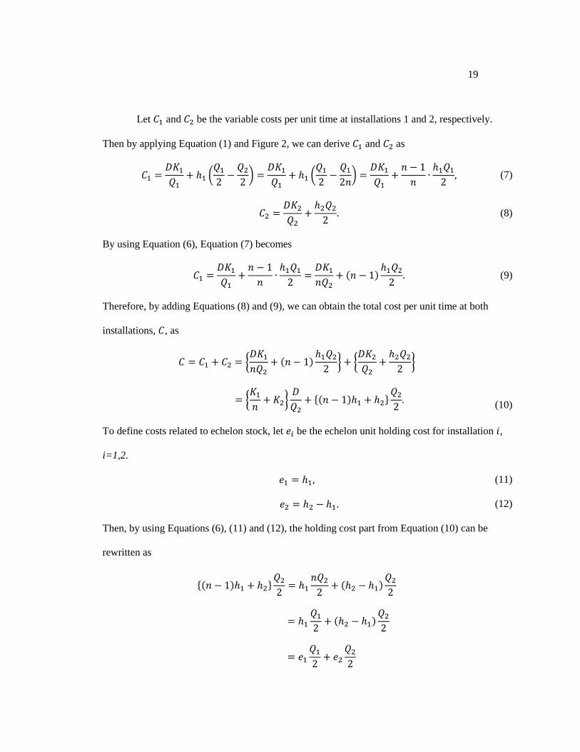
Let and be the variable costs per unit time at installations 1 and 2, respectively.
Then by applying Equation (1) and Figure 2, we can derive and as
(
)
(
)
(7)
(8)
By using Equation (6), Equation (7) becomes
(9)
Therefore, by adding Equations (8) and (9), we can obtain the total cost per unit time at both
installations, , as
{
} {
}
{
}
{ }
(10)
To define costs related to echelon stock, let be the echelon unit holding cost for installation ,
i=1,2.
(11)
(12)
Then, by using Equations (6), (11) and (12), the holding cost part from Equation (10) can be
rewritten as
{ }

20
(13)
By using Equation (13), we can paraphrase Equation (10) as
{
}
{ }
{
}
{ }
(14)
Since the inventory at a manufacturer is used to replenish the inventory at a distribution center in
a supply chain, the optimal order quantity at installation 1 for a manufacturer, , is determined
after finding the optimal order quantity at installation 2 for a distribution center, . Thus, we
calculate first, then
can be easily derived by Equation (6). In order to find , we take
the derivative with respect to from Equation (14), as follows.
{
}
(15)
Then setting Equation (15) to zero, and solving it for yields
√
{ }
(16)
Also, by using Equations (6) and (16), we can calculate as
√ {
}
, : fixed positive integer.
(17)
Now by replacing in Equation (14) by the expression in Equation (16), the minimum total
cost per unit time for the deterministic serial two-echelon system, , is derived as
{
}
{ }

21
{
} √
{ }
{ }
√ {
}
√ (
)
(18)
These results in Section 3.3 are going to be a basis to do robust analysis and derive the
method for the deterministic serial two-echelon inventory model in a supply chain.
22
Chapter 4
ROBUST ANALYSIS
The background inventory models summarized in Chapter 3 are working well on the
assumption that all the parameters are known and deterministic. In a real-world inventory
problem, however, there is a slight chance to know the exact values of all the parameters because
their values are frequently affected by economic environments (Gallego et al. 2001). When values
of all the parameters are not certain, we classify this inventory problem as two categories, such as
(i) risk; and (ii) uncertainty (Snyder 2006). If there exist uncertain parameters whose values
follow known probability distributions, this inventory problem is categorized as a risk situation,
and is approached from a stochastic perspective. But in the real-world inventory problem, it is
also hard to know probability distributions of uncertain parameters. In this case, we assume that
all the parameters are uncertain and any information about probability distribution of all the
parameters is also unknown. We categorize this into uncertain situation. A problem under
uncertain situation is often regarded as robust optimization problem view, and uncertainty of each
parameter is described as a continuous value that is restricted to some prespecified interval
(Rosenhead et al. 1972).
In this chapter, we assume that all the parameters are unknown with some prespecified
intervals. Then from a robust optimization point of view, we analyze the effect of each
parameter’s randomness to the basic EOQ model and the deterministic serial two-echelon
inventory model, introduced in Chapter 3. Since this thesis considers analysis based on input data
uncertainty, we call it robust analysis. This thesis has three objectives. The first goal is to develop
closed form expressions for the basic EOQ’s model to characterize the set consisting of all
23
possible EOQ’s and corresponding minimum average costs. In order to achieve this goal, Section
4.1 considers all the possible combinations of the basic EOQ parameters (D, K, and h) under their
prespecified intervals. By investigating all the possible values from each combination of D, K,
and h, we derive interval of EOQ and the upper and lower bounds of minimum average cost for
each EOQ. Thus, we can derive two closed form functions for the upper and lower bounds of
minimum average cost. By considering these two functions together, we obtain the closed form
expressions which characterize the set of all possible EOQ’s and corresponding minimum
average costs when all the parameters are unknown.
The second goal of this thesis is to analyze the effect of randomness in the worst case for
all EOQs and suggest the closed form optimal order policy in which this worst case is minimized.
In order to reach this goal, Section 4.2 suggests two minimax analyses – the ratio approach and
the difference approach. These two minimax analyses are used to find the optimal order policy to
minimize the worst error, thus the concept of the ratio approach is same to the concept of
difference approach, which is to find the worst error and then make it minimize. But the
definition of the error is different between the ratio approach and the difference approach. The
ratio approach defines the error as a ratio of a feasible average cost to the minimum average cost,
while the difference approach defines the error as a difference between a feasible average cost
and the minimum average cost. Thus, regarding the closed form expression which analyzes the
effect of randomness in the worst case for all EOQs, the ratio approach has a different closed
form expression from a difference approach has. Also, regarding an optimal order policy that
produces the lowest possible error, the ratio approach suggests that the geometric mean of the
maximum and the minimum EOQ’s is optimal, while the difference approach proposes the
arithmetic mean of the maximum and the minimum EOQ’s as the optimal order policy.
Last but not the least, the final goal of this thesis is to find the best multiplicity factor to
minimize upper bound of the minimum total cost of the deterministic serial two-echelon

24
inventory model. In order to attain this goal, Section 4.3 extends the closed form expressions
derived in Section 4.1 to the deterministic serial two-echelon inventory model. Two-echelon
inventory model has the multiplicity factor for order quantity between echelons, but the
multiplicity factor complicates the problem. Thus, in Section 4.3.1, we first derive the closed
form expressions that characterize the set of all possible optimal order quantities and
corresponding minimum total costs for the two-echelon inventory model when the multiplicity
factor is fixed. However, the multiplicity factor actually takes different positive integers under
input data uncertainty. Thus, in Section 4.3.2, we obtain all the possible multiplicity factors, and
apply our closed form expressions to each multiplicity factor. By doing this, we find the best
multiplicity factor at which upper bound of the minimum total cost of the two-echelon inventory
model is minimized.
4.1 Robust Analysis of the Basic EOQ Model
In this section, we are interested in the set of minimum average costs depending on
intervals of the optimal order quantity, derived from the following intervals of D, K, and h. That
is, we assume that true values of D, K, and h are unknown without any probability distributions
for them, but we can approximate their intervals only as
(19)
As seen in Equation (3), the optimal order quantity increases when D or K increases or when h
decreases. Thus, given the above intervals, the largest value of the optimal order quantity, , is

25
√
(20)
and the smallest value of the optimal order quantity, , is
√
(21)
On the other hand, the minimum average cost, , increases when D, K or h increases by
Equation (4). Similarly, decreases if D, K or h decreases by Equation (4). Thus, we can
infer that is minimized when all of D, K, and h have their lowest values in Intervals (19).
We define as the optimal order quantity at which is minimized. By applying Equation
(4), we can derive as
√
(22)
Similarly, we define as the optimal order quantity at which is maximized. We can also
derive by using Equation (4) as
√
(23)
Since the values of and
depend on the intervals of D, K, and h, it is generally hard to
distinguish which one is always greater than the other one. According to the intervals of D, K,
and h, sometimes can be greater than
, and sometimes would be larger than
. Thus,
by Equations (20) – (23), the intervals of for general inventory model is
[
]
[
] (24)
Note that we can have different combinations of D, K, and h under uncertainty about
their values. Thus, by Equation (3), different can be derived from different combinations of D,
K, and h, and it can also have different by Equation (4). Now, we want to know the upper

26
and lower bounds of according to . We denote the upper and lower bounds of as
and , respectively. As a part of deriving the equations of and
, we can rewrite Equation (3) in terms of D and K. The equation is
(25)
Then, by replacing D and K in Equation (1) by Equation (25), we can rewrite Equation (1) as
(26)
To find upper bound of , we fix as , then by Equation (3), √
,
[ ], [ ], and is always between and
by Equations (21) and (23),
i.e.,
. Thus, fixing as in Equation (26), the equation of over
is
,
(27)
As we did in Equation (25), we can also rewrite Equation (3) in terms of , then the equation is
(28)
Also, by substituting
for in Equation (1), we can rewrite Equation (1) as
(29)
Similarly, to find upper bound of , we fix and as and , then by Equation (3),
√
, [ ], and is always between
and by Equations (23) and (20),
i.e.,
. Thus, fixing D and K as and in Equation (29), now the equation of
over
is
,
(30)

27
Therefore, Equations (27) and (30) are upper bound of the minimum average cost, , that
is,
{
(31)
Note that increases monotonically over
, then decreases monotonically
over the next interval,
. Figure 3 describes Equation (31) according to different set
of .
Figure 3. Upper bound of the set of the minimum average costs
As obtained, we can also obtain lower bound of the minimum average cost,
, in the same way. Now, to find , we fix and as and , then by
Equation (3), √
, [ ], and is always between
and by Equations
√
√
√
√

28
(21) and (22), i.e.,
. Thus, by fixing D and K as and in Equation (29), the
equation of over
is
,
(32)
Also, to find , we fix h as , then by Equation (3), √
, [ ],
[ ], and is always between and
by Equations (22) and (20), i.e.,
.
Thus, by fixing h as in Equation (26), we can determine the equation of over
. It is written as
,
(33)
Therefore, lower bound of the minimum average cost, , which consists of Equation (32)
and (33), is
{
(34)
On the contrary to , decreases monotonically over
, then
increases monotonically over the next interval,
. Figure 4 describes Equation (34)
according to different set of .

29
Figure 4. Lower bound of the set of the minimum average costs
By considering Figures 3 and 4 together, we can figure out how the upper and lower
bounds of change over the intervals of . Since the minimum average costs are only
defined over
, an order quantity should not go beyond the interval,
,
when we know the intervals of D, K, and h. Figure 5 shows the combination of the upper and
lower bounds of . It is meaningful because it describes the set of all possible EOQ’s and
corresponding minimum average costs. We call it a feasible optimal region of the basic EOQ
model.
Definition. A feasible optimal region of the basic EOQ model is the set of all possible EOQ’s
and corresponding minimum average costs of the basic EOQ model if all parameters are
uncertain, and furthermore, no information about their probability distribution is provided, but
√
√
√
√

30
these values are only restricted to some prespecified intervals. The feasible optimal region
indicates variability of EOQ and minimum average cost under input data uncertainty.
Figure 5. Feasible optimal region of the basic EOQ model
Note that it would not be easy to obtain intervals of the parameters even if we assumed
that each value is restricted to some prespecified interval. It indicates that these prespecified
intervals, such as Intervals (19), can be generally obtained through estimation, and the upper and
lower bounds of these intervals can have some error. Besides, these prespecified intervals could
change, meaning that the upper bound or the lower bound of each parameter could change. Thus,
we can expect that these intervals affect the feasible optimal region. For example, if the value of
changes, then only the upper bound between
also changes by Equation (31),
but the other parts remain same in the current feasible optimal region. Another example is when
only the value of changes but the other prespecified intervals remain same. In this case, only
√
√
√
√

31
the lower bound between
also changes by Equation (34), but the other parts do
not change at all in the current feasible optimal region. Similarly, if only the values of and
change but the other prespecified intervals remain same, only the lower bound between
and the upper bound between
also change by Equations (34) and (31),
respectively. These examples build the general conclusion that each interval only affects the part
whose closed form expression relates to this interval in the feasible optimal region. We discuss it
more with a numerical example (Figure 14) at the end of Section 5.1.
Under the feasible optimal region on Figure 5, derived by , , and would be
the best order quantity because its minimum average cost is the lowest in the whole feasible
optimal region. However, the problem is that it is hard for a manager to know the exact values of
the parameters, and the manager needs to estimate their values, that may include errors between
the real values and the estimated values. For example, an inventory manager estimates that the
values of D, K, and h are , , and , respectively, and then the manager makes a decision to
order because
is optimal to produce the lowest minimum average cost at , , and .
However, if his estimation is wrong and the real values of D, K, and h are actually , , and
, respectively, then minimum average cost at will not become the lowest. That is, the
manager estimates that the minimum average cost at is
by applying Equation
(1), or equivalently from Equation (33). But, the true average cost at
is actually
, which is larger than expected. Note that the lower bound of the minimum
average cost is when the real values of D, K, and h are , , and . Since there exists a
big difference between and
, the manager may want to avoid the risk as much as
possible in risk-averse view even if he makes a wrong decision. Thus, Section 4.2 focuses on how
to minimize this risk. In order to do that, we compare estimated, feasible average costs to the

32
minimum average cost in two ways; a ratio and a difference between feasible average costs and
the minimum average cost.
4.2 Minimax Analysis of the Basic EOQ Model
At the end of Section 4.1, we briefly introduced a motivation of minimizing the worst
error. We would expect the minimum average cost at when D, K, and h are estimated as ,
and , respectively. However, if the real values of D, K, and h are completely different from
the estimates of D, K, and h, we will face against a bad case, meaning that the true minimum
average cost may be much higher than the minimum average cost at . It could cause
undesirable high-risk. Thus, in Section 4.2, we want to analyze the effect of randomness in the
worst case scenario, and find the closed form optimal order policy that produces the smallest
possible error in the worst case through two minimax frameworks; minimizing the worst error
ratio and minimizing the worst error difference. The first approach is to minimize the worst error
ratio of a feasible average cost to the minimum average cost, and the second one is to minimize
the worst error difference between a feasible average cost and the minimum average cost. We
start our idea with the worst error ratio first.
4.2.1 The ratio approach to minimize the worst error
We obtain the interval of from equations (20) – (24),
. Let be an
order quantity decided by a manager. A manager believes equal to , thus the interval of is
also between and
. Now, we need to define ( ) compared to . ( ) denotes an
actual average cost at which is decided by a manager by wrong approximates of D, K, and h,
whereas denotes the minimum average cost at by true values of D, K, and h. Let ( )
33
be a function of the worst error ratio of a feasible average cost to the minimum average cost.
Since our objective is to minimize ( ), we define our minimax objective function as
( )
{
( )
} (35)
To find an optimal point ,
, which minimizes the worst error ratio, as expressed
by equation (35), the two following steps are suggested.
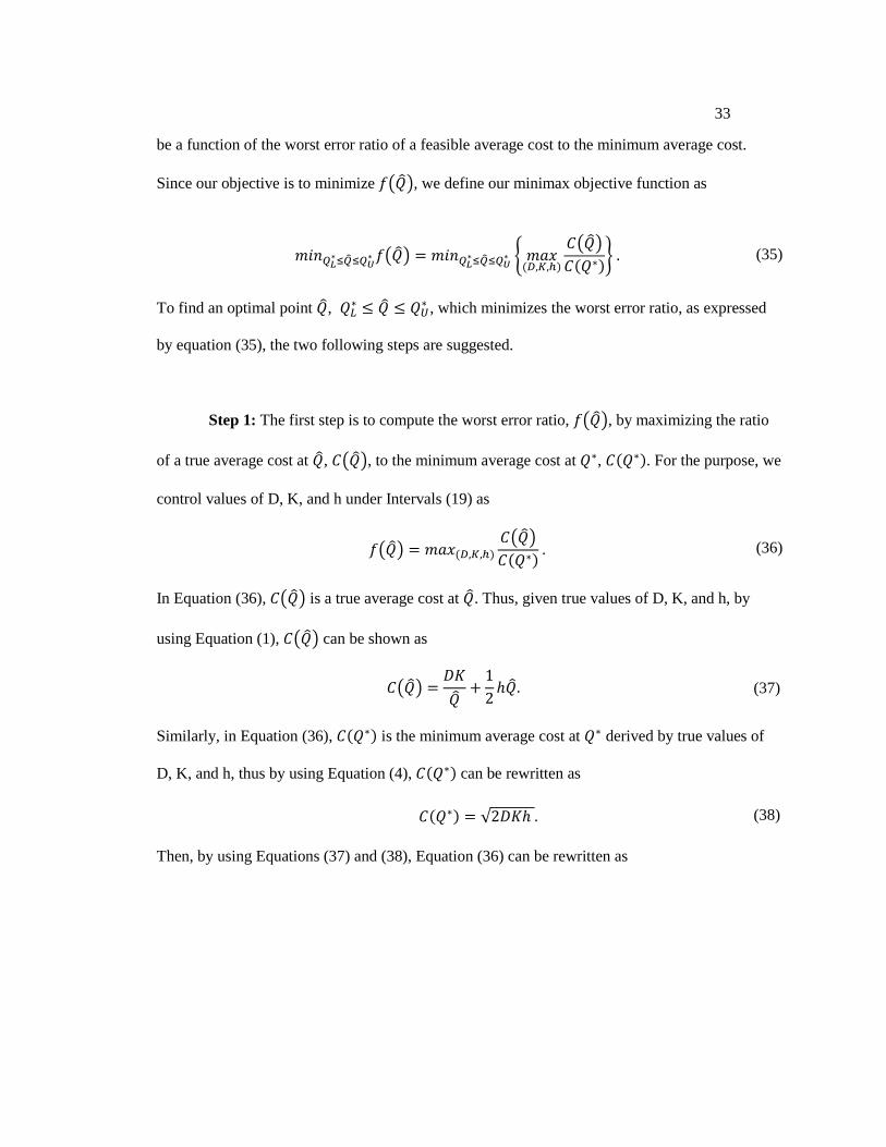
Step 1: The first step is to compute the worst error ratio, ( ), by maximizing the ratio
of a true average cost at , ( ), to the minimum average cost at , . For the purpose, we
control values of D, K, and h under Intervals (19) as
( )
( )
(36)
In Equation (36), ( ) is a true average cost at . Thus, given true values of D, K, and h, by
using Equation (1), ( ) can be shown as
( )
(37)
Similarly, in Equation (36), is the minimum average cost at derived by true values of
D, K, and h, thus by using Equation (4), can be rewritten as
√ (38)
Then, by using Equations (37) and (38), Equation (36) can be rewritten as

34
( )
{ ( )
}
{
√ }
{
√
√
}
{
√
√
}
{
}
{
(
)}
(39)
Equation (39) shows ( ) is a convex function, and we can find the maximum value of ( ) at
or
Therefore, Equation (39) can be rewritten as
( )
{ ( )
}
(
){
(
)}
{
(
)
(
) }
{ },
where
(
),
(
)
(40)
To simplify Equation (40), as seen above, “ ” denotes
(
) and “ ” denotes
(
).
Since Equation (40) can have a different result according to the values of , and
, we need
to consider both of the two following cases for Equation (40) as
{ { } { }
(41)
For example, by Equation (41), Case 1 represents “ ” is greater than or equal to “ ”, but since
the replaced letters of “ ” and “ ” are not intuitive to understand the model, we need to specify

35
each of these two cases by using Equation (40). Let us keep going with Case 1, i.e.,
{ } . This implies that
(
)
(
)
(
)
(
)
( )
√
(42)
Thus, “ { } ” in Equation (41) implies √
. Similarly, Case 2 in Equation
(41) can be rewritten as √
. To sum up,
{ { } √
{ } √
(43)
In the next step, we want to find ,
, to solve the original equation (35) that
minimizes the worst error ratio.
Step 2: Now in this step, we consider both of the two cases of √
and
√
to find , at which Equation (40) is minimized and it finally suggests a solution to
minimize the worst error ratio.

36
(1) Case 1: √
When √
, Equation (40) is equal to
(
). Thus, in this case we can
rewrite Equation (35) as
√
( )
√
{
( )
}
√
{
(
)}
(44)
(
) is a steadily decreasing function in the interval of
√
because it
satisfies the condition that for , where and are any two values in the
interval. Thus, its minimum value occurred at √
, that is,
√
, for √
(45)
Hence, Equation (45) shows that √
has to be selected to minimize the worst error ratio in
case of √
.
(2) Case 2: √
When √
, now Equation (40) is equal to
(
). Thus, in this case we
can rewrite Equation (35) as
√
( )
√
{
( )
}
√
{
(
)}
(46)

37
Now,
(
) is a steadily increasing function in the interval of √
because
it satisfies the condition that for , where and are any two values in the
interval. Thus,
(
) has a minimum value at √
, meaning that this is the same
result to Case 1, that is,
√
, for √
(47)
Hence, Equation (47) supports that √
also has to be selected to minimize the worst error
ratio in case of √
.
Because Equations (45) and (47) have the same optimal solution to minimize the worst
error ratio, ( ), we can generally conclude that √
in the interval of
,
where denotes the optimal order quantity that minimizes the worst error ratio. Note that the
value of is equal to the geometric mean of the maximum and the minimum EOQ’s. Figure 6
illustrates how the worst error ratio is minimized at the geometric mean of the maximum and the
minimum of EOQ’s.

38
Figure 6. Effect of randomness in the worst error ratio
4.2.2 The difference approach to minimize the worst error
In Section 4.1, we found that ( ) is minimized at √
, meaning that the
worst error ratio is minimized at the geometric mean of the maximum and the minimum EOQ’s.
Similar to Section 4.2.1, let ( ) be a function of the worst error difference between a feasible
average cost and the minimum average cost. Now our goal is to minimize ( ), thus we can
define our minimax problem as
( )
[ { ( ) }] (48)
Like the procedure which we did in Section 4.2.1, the worst error difference between a feasible
average cost and the minimum average cost can be derived through the two steps, as follows.
( )
√
√
√

39
Step 1: First, we need to solve the worst error difference, ( ), by maximizing the
difference between a true average cost at , ( ), and the minimum average cost at , .
For the purpose, we control values of D, K, and h under Intervals (19) as
( ) { ( ) } (49)
Since ( ) is a true average cost at and is a minimum average cost at , we can
rewrite Equation (49) by using Equations (37) and (38) as
( )
{ ( ) }
{
√ }
{
√
}
{
}
[ {
}]
(50)
Since is the minimum average cost, ( ) is always greater than or equal to . Thus,
Equations (49) and (50) are always positive or zero. Besides, in Equation (50) is the inventory
holding cost per unit per unit time and it always has a positive value. This implies that {
} in Equation (50) is also always greater than or equal to zero. Thus, the value of should
be to maximize Equation (50). Then, Equation (50) can be rewritten as
( )
{ ( ) }
[ {
}]
[ {
}]
(51)
40
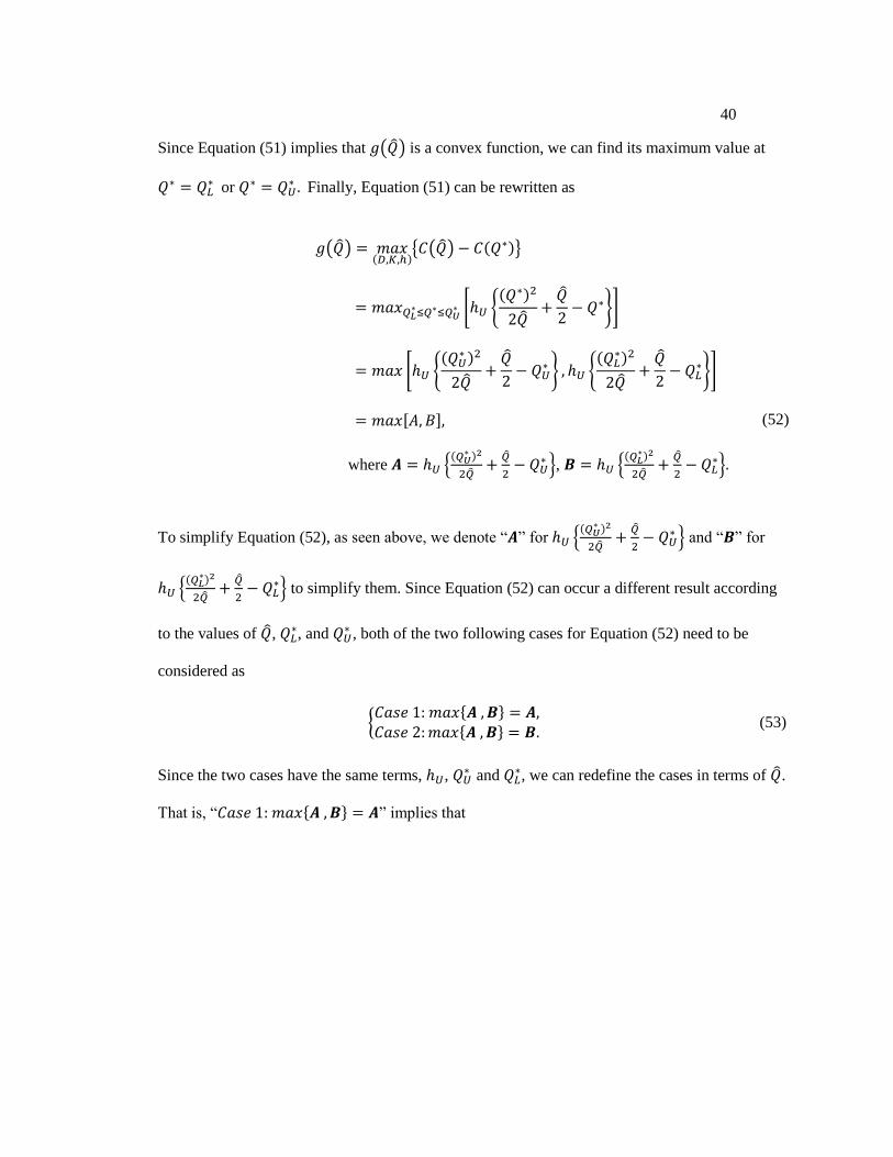
Since Equation (51) implies that ( ) is a convex function, we can find its maximum value at
or
Finally, Equation (51) can be rewritten as
( )
{ ( ) }
[ {
}]
[ {
} {
}]
[ ]
where {
}, {
}
(52)
To simplify Equation (52), as seen above, we denote “ ” for {
} and “ ” for
{
} to simplify them. Since Equation (52) can occur a different result according
to the values of , , and
, both of the two following cases for Equation (52) need to be
considered as
{ { } { }
(53)
Since the two cases have the same terms, , and
, we can redefine the cases in terms of .
That is, “ { } ” implies that

41
{
} {
}
(54)
Thus, “ { } ” in Equation (53) implies
. Similarly, Case 2 in Equation
(53) can be rewritten as
. To sum up,
{ { }
{ }
(55)
Step 2: In this step, we want to find to minimize the worst error difference, ( ),
between a true average cost at and the minimum average cost at in the original equation
(48). The first case is
, and the second case is
.
(1) Case 1:
When
, Equation (52) is equal to {
}. Thus, Equation (48)
can be rewritten as

42
( )
[
( ) ]
[ {
}]
(56)
{
} is a steadily decreasing function in the interval of
because it satisfies the condition that for , where and are any two values
in the interval. Thus, its minimum value occurred at
, that is,
(57)
Hence, Equation (57) shows that
has to be selected to minimize the worst error difference
in case of
.
(2) Case 2:
Similarly, when
, Equation (52) is now equal to {
}. Then
we can rewrite Equation (48) by using {
} as
( )
[
( ) ]
[ {
}]
(58)
{
} is a steadily increasing function in the interval of
because
it satisfies the condition that for , where and are any two values in the
interval. Thus, this function has the minimum value at
, which is the same result to
Case 1, that is,
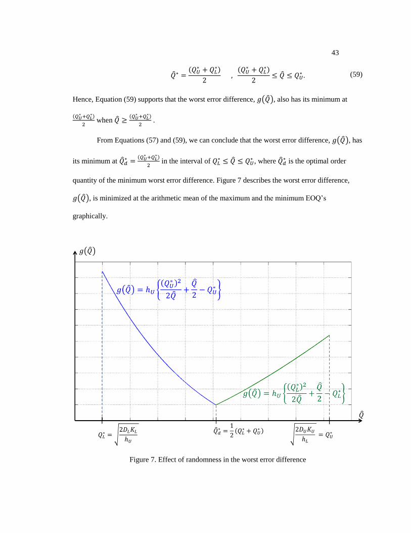
43
(59)
Hence, Equation (59) supports that the worst error difference, ( ), also has its minimum at
when
.
From Equations (57) and (59), we can conclude that the worst error difference, ( ), has
its minimum at
in the interval of
, where
is the optimal order
quantity of the minimum worst error difference. Figure 7 describes the worst error difference,
( ), is minimized at the arithmetic mean of the maximum and the minimum EOQ’s
graphically.
Figure 7. Effect of randomness in the worst error difference
( )
√
√

44
A manager wants to avoid the most undesirable loss comparing to its minimum average
cost. From Sections 4.2.1 and 4.2.2, we found two optimal order quantities to minimize the worst
error situation. In Section 4.2.1, the worst error ratio of a feasible average cost to its minimum
average cost is minimized at
√
,
(60)
On the other hand, the worst error difference between a feasible average cost and the minimum
average cost is minimized at
,
(61)
Equation (60) implies that the worst error ratio can be minimized at the geometric mean of the
maximum and the minimum EOQ’s. On the other hand, Equation (61) implies that the worst error
difference can be minimized at the arithmetic mean of the maximum and the minimum EOQ’s.
Thus, a manager properly needs to decide how many quantities are ordered to minimize risk in
two different views, ratio or difference comparing to the minimum average cost. Note that the
geometric mean, , is always less than or equal to the arithmetic mean,
. Thus, can be
selected if setup cost is relatively higher than other costs. On the other hand, when an inventory
holding cost occupies a larger portion than setup cost does, can be a better choice.
4.3 Robust Analysis of the Deterministic Serial Two-Echelon Inventory Model
In this section, we extend our robust analysis of the basic EOQ model to deterministic
serial two-echelon inventory model in a supply chain. Like doing robust analysis of the basic
EOQ model in Section 4.1, the classic assumption that the values which compose the
deterministic serial two-echelon inventory model are known and fixed is relaxed in this section.
Instead, now we can only approximate rough intervals of their values as

45
,
,
,
,
.
(62)
If we have Intervals (62), the upper and lower bounds of can be derived by using Equation (11)
as
, where and
.
(63)
Similarly, the upper and lower bounds of can also be calculated by using Equation (12), that is,
, where and
(64)
It is clear that Interval (63) is always positive, since lower bound of equals and cannot
be negative. To check if Interval (64) is also positive all the time, we need to review the third
assumption in Section 3.3. According to that assumption, is always greater than because
units increase in value from installation 1 to installation 2. Thus, it is reasonable that lower bound
of is still greater than upper bound of provided , that is,
(65)
Inequality (65) finally guarantees that Interval (64) is also always positive. Therefore, we can say
that all the parameters defined for the deterministic serial two-echelon inventory model have
positive sets.
One of the main characteristic of the deterministic serial two-echelon inventory model is
that it has the multiplicity factor, denoted as , for order quantity between echelons. The
46
multiplicity factor was explained in Section 3.3, and its optimal value can be obtained by taking
the derivative of Equation (18) inside the square root, setting this derivative equal to zero and
solving for . But the parameters such as , , , and , which affect the optimal value of
multiplicity factor, are unknown in this thesis. This makes the multiplicity factor also unknown,
and it complicates our robust analysis of the two-echelon inventory model. For example, when
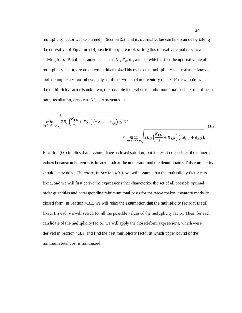
the multiplicity factor is unknown, the possible interval of the minimum total cost per unit time at
both installation, denote as , is represented as
√ (
) ( )
√ (
) ( )
(66)
Equation (66) implies that it cannot have a closed solution, but its result depends on the numerical
values because unknown is located both at the numerator and the denominator. This complexity
should be avoided. Therefore, in Section 4.3.1, we will assume that the multiplicity factor is
fixed, and we will first derive the expressions that characterize the set of all possible optimal
order quantities and corresponding minimum total costs for the two-echelon inventory model in
closed form. In Section 4.3.2, we will relax the assumption that the multiplicity factor is still
fixed. Instead, we will search for all the possible values of the multiplicity factor. Then, for each
candidate of the multiplicity factor, we will apply the closed-form expressions, which were
derived in Section 4.3.1, and find the best multiplicity factor at which upper bound of the
minimum total cost is minimized.
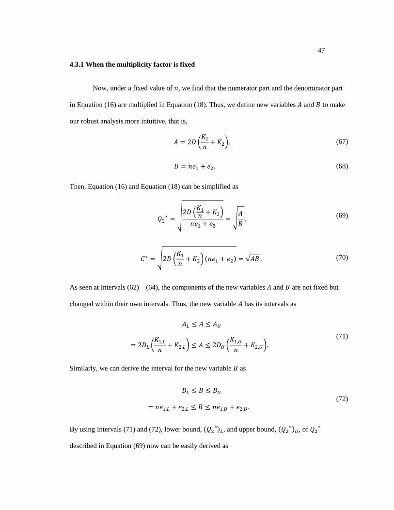
47
4.3.1 When the multiplicity factor is fixed
Now, under a fixed value of , we find that the numerator part and the denominator part
in Equation (16) are multiplied in Equation (18). Thus, we define new variables and to make
our robust analysis more intuitive, that is,
(
) (67)
(68)
Then, Equation (16) and Equation (18) can be simplified as
√
( )
√
(69)
√ (
) √ (70)
As seen at Intervals (62) – (64), the components of the new variables and are not fixed but
changed within their own intervals. Thus, the new variable has its intervals as
(
) (
)
(71)
Similarly, we can derive the interval for the new variable as
(72)
By using Intervals (71) and (72), lower bound, , and upper bound,
, of
described in Equation (69) now can be easily derived as

48
√
√ (
)
(73)
√
√ (
)
(74)
Similarly, by using Intervals (71) and (72), we can have an interval for Equation (70) as
√ √
√ (
) ( ) √ (
) ( )
(75)
From Interval (75), we can find the specific optimal order quantity of the second installation
at which the minimum total cost is minimized, as follows.
√
√ (
)
(76)
In the same way, the specific optimal order quantity of the second installation at which
the minimum total cost can have its maximum is
√
√
(
)
(77)
As we discussed in Section 4.1 for the basic EOQ model, the values of and
depend on Intervals (62) – (64). Thus we cannot guarantee which value is always greater than the
other between and
, but it is clear that the interval of includes both
and , that is,
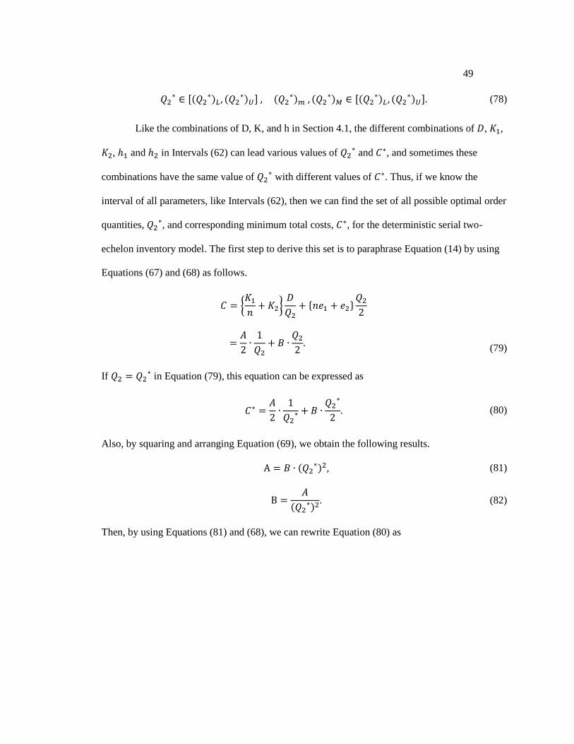
49
[
]
[
] (78)
Like the combinations of D, K, and h in Section 4.1, the different combinations of , ,
, and in Intervals (62) can lead various values of and , and sometimes these
combinations have the same value of with different values of . Thus, if we know the
interval of all parameters, like Intervals (62), then we can find the set of all possible optimal order
quantities, , and corresponding minimum total costs, , for the deterministic serial two-
echelon inventory model. The first step to derive this set is to paraphrase Equation (14) by using
Equations (67) and (68) as follows.
{
}
{ }
(79)
If in Equation (79), this equation can be expressed as
(80)
Also, by squaring and arranging Equation (69), we obtain the following results.
(81)
(82)
Then, by using Equations (81) and (68), we can rewrite Equation (80) as

50
(83)
Or equivalently, by using Equations (82) and (67), Equation (80) can be rewritten as
(
)
(84)
Now, as to find the former part of upper bound of , we first fix the value of as ,
then by Equation (69), √
, [ ]. In this case, the domain
is placed between
and
by Equations (73) and (77), i.e.,
. This implies that
fixing the value of as makes Equation (83) over
as
( ) ,
(85)
Next, we fix the value of as in order to find the latter part of upper bound of . Then by
Equation (69), √
, [ ]. In this case, by Equations (77) and (74), the domain
lies between
and , that is,
. Thus, Equation (84) with
a fixed value of over
is

51
(
)
,
(86)
Therefore, we can obtain upper bound of the minimum total cost per unit time for the
deterministic serial two-echelon system, , by combining Equations (85) and (86) as
{
( )
(
)
(87)
Equation (87) has an increasing linear function over the former part,
,
then it has a decreasing fractional function over the latter part,
. Figure 8
illustrates these characteristics of Equation (87).
Figure 8. Upper bound of the set of the minimum total costs

52
Similarly, lower bound of can be created by combining the former part and the latter
part of lower bound of . First, to obtain the former part of lower bound, we fix the value of as
. Then by Equation (69), √
, [ ]. In this case, we can infer that the domain
is placed between
and by Equations (73) and (76), in other words,
. Thus, Equation (84) with a fixed value of over
can
be expressed as
(
)
,
(88)
The next thing is to derive the latter part of lower bound by fixing the value of as , then by
Equation (69), √
, [ ]. In this case, by Equations (76) and (74), the domain
is located between
and , or equivalently,
. This
represents Equation (83) with a fixed value of over
is
( ) ,
(89)
Now we put Equations (88) and (89) together and draw lower bound of the minimum total cost
per unit time for the deterministic serial two-echelon system, , as
{
(
)
( )
(90)

53
Figure 9 graphically shows that Equation (90) has a decreasing fractional function over the
former part,
, then it has an increasing linear function over the latter part,
.
Figure 9. Lower bound of the set of the minimum total costs
By considering the upper and lower bounds of together into one plot, we can finally
describe the set of all possible optimal order quantities, , and corresponding minimum total
costs, , for the deterministic serial two-echelon model. Since this set describes all possible
inventory situations under input data uncertainty, we call this set a feasible optimal region of the
deterministic serial two-echelon inventory model in this thesis.
Definition. A feasible optimal region of the deterministic serial two-echelon inventory model is
the set of all possible optimal order quantities and corresponding minimum total costs if all

54
parameters are uncertain, and furthermore, no information about their probability distribution is
provided. The feasible optimal region indicates variability of optimal order quantity and
minimum total cost under input data uncertainty.
Figure 10 shows the feasible optimal region, created by combining the figures 8 and 9
together.
Figure 10. Two-dimensional feasible optimal region of the deterministic serial two-echelon
inventory model
Since our robust analysis is for the deterministic serial two-echelon model, we also need
to be considered for the feasible optimal region of , as well as
. To do that, we first
need to calculate lower bound, , and upper bound,
, of by using Equations (17),
(73) and (74), as follows.

55
√
√ (
)
(91)
√
√ (
)
(92)
Now we have all the intervals both for and
, and we can infer the relation between
and by using Equation (17), thus we can finally draw a three-dimensional feasible optimal
region of the minimum total cost for the deterministic serial two-echelon system over the
intervals of and
. Note that this feasible optimal region should be three-dimensional since
affects
and finally affects . Figure 11 plots this three-dimensional feasible optimal
region while both and
change within their intervals. The feasible optimal region is useful
because it is almost impossible to find the exact values for all parameters and these parameters
change their values frequently or continuously by the diverse economic factors. When we only
knows rough intervals of the parameters, we can derive various optimal solutions according to
different combinations of the parameters, thus the feasible optimal region is meaningful in the
way that it describes all the possible optimal solution sets.

56
Figure 11. Three-dimensional feasible optimal region of the deterministic serial two-echelon
inventory model
By observing Figure 11, we can figure out how many optimal order quantities at a manufacturer
and a distribution center can directly affect the minimum total cost in the deterministic serial two-
echelon supply chain when we only know rough intervals of the parameters like Intervals (62),
and furthermore we can cope actively with the changing situations on the basis of this analysis.
The parameters which compose the deterministic serial two-echelon inventory model
have changeable values in the various environments, and it is generally hard to predict their
values exactly. In this situation, all the manager can know at his best would be their rough
intervals like Intervals (62), but he may fail to control these values. The one thing he can control
is the multiplicity factor in Equation (6). Since is the fixed positive integer that indicates
supply chain contract, such as transportation restriction condition or storage space constraint, the
manager can adjust this value when he makes or renews contract. Thus, in Section 4.3.2 we will
assume that the manager can take various multiplicity factors. In this part we will first calculate

57
all the candidates of the optimal multiplicity factor under input data uncertainty then we will
analyze the effect of each multiplicity factor to the feasible optimal region as the number of
optimal multiplicity factors goes to large. We expect that a large value of the multiplicity factor is
attractive in the way that it can decrease the variability of the minimum total cost. Note that the
difference between and
can decrease by Equations (73) and (74) as the
multiplicity factor increases,. Figure 12 shows {
} decreases logarithmically as
goes to large.
Figure 12. Logarithmically decreasing relationship between the interval of the optimal order
quantity at installation 2 and the multiplicity factor
Also, from Equations (17) and (18), we can infer has a direct influence on
and . Thus
controlling the interval of represents we can also control the size of a three-dimensional
feasible optimal region of the minimum total cost for the deterministic serial two-echelon system.
{
}

58
One problem is, however, it is impossible to increase the value of to the infinity practically.
Thus, the manager needs to make or renew contract with the large value of at its practical level
to reduce the interval of and to reduce the size of the three-dimensional feasible optimal
region.
4.3.2 When the multiplicity factor is not fixed
To analyze the effect of the multiplicity factor to the feasible optimal region, now we
consider all the candidates of . First, we can obtain the optimal multiplicity factor, , by taking
the derivative of Equation (18) inside the square root, setting this derivative equal to zero and
solving for . That is,
{ }
{ (
) }
(
)
√
(93)
But in this section, , , and change within their intervals. Thus, we can also obtain lower
bound, , and upper bound, , of the optimal multiplicity factor by using Equation (93),
as follows.

59
√
√
(94)
Since the multiplicity factor is a positive integer, we can investigate the interval of and the
interval of for each positive integer in Interval (94). Then we can find the best positive
integer at which and are minimized among all possible s. The following method is
the summary how we can find the best multiplicity factor when is not fixed.
Step 1. Calculate the interval of , i.e.,
√
√
Step 2. For each positive integer in the interval above, investigate ,
,
,
, , , and
, draw the feasible
optimal region, and calculate its area.
Step 3. Among the all positive integers s, find the best at which is
minimized with small area of the feasible optimal region.
In Section 5.3, we are going to apply this method to the numerical example and find the
best at which upper bound of the minimum total cost, , is minimized with small area of
the feasible optimal region.

60
Chapter 5
NUMERICAL EXAMPLES
In this chapter, we provide numerical examples to help understand our robust analyses of
the basic EOQ model and deterministic serial two-echelon inventory model in a supply chain
treated at Chapter 4 when we do not know the exact values of the parameters that compose the
models but we only know their rough intervals.
5.1 A Numerical Example for Robust Analysis of the Basic EOQ Model
In this section, we talk about a numerical example for the basic EOQ model, and we
explain how to draw the minimum average costs according to . The numerical example to be
used for the basic EOQ model is based on Schwarz’s work (Schwarz, 2008). Like Schwarz’s
numerical example in his paper, we do not know the exact values of D, K, and h but only know
their rough intervals on the following:
(95)
Based on Intervals (95), we can find the feasible optimal region composed of optimal order
quantities and their minimum average costs according to the different combinations of D, K, and
h. As a first step, by using Equations (20) and (21), lower bound of the optimal order
quantity, , and upper bound of the optimal order quantity,
, are computed as

61
√
√
√
√
(96)
and by using Equations (22) and (23), we can calculate and
as
√
√
√
√
(97)
Then by replacing ,
, , and
in Equations (31) and (34) by the numbers obtained in
Equations (96) and (97), we can have the upper and lower bounds of the minimum average cost,
as follows.
{
(98)
{
(99)
By using Equations (98) and (99), we can finally draw the feasible optimal region as Figure 13.
The feasible optimal region is meaningful in the way that it describes the whole possible optimal
set of minimum average costs according to the different combinations of D, K, and h when we do
not have the information about the exact values of D, K, and h but only have their rough intervals.
In real life inventory problem, it is difficult to predict the exact values of D, K, and h. Besides,
even if we derive the exact values, these values would be easily affected and changed by the
various economic factors. Thus, the feasible optimal region derived by the certain intervals of D,
K, and h can be more worthy and can allow us to be fully aware of what to do when the values
are continuously changed within their estimated intervals.

62
Figure 13. Four expressions to describe the feasible optimal region of the basic EOQ model
Now, let us consider the case where the upper bound or the lower bound of Intervals (95)
changes. Figure 14 describes how these intervals affect the original feasible optimal region.
Figure 14 – (a) describes the original feasible optimal region by Intervals (95), which is equal to
Figure 13. Figure 14 – (b) only changes the value of from to , but the other
intervals remain same. As a result, and
change from and to and
by Equations (97) and (96), respectively. Also, because has an effect on the upper
bound between
by Equation (31), only the upper bound between
changes from (
) to (
) by applying Equation (98), but the
other parts remain same in the original feasible optimal region. Similarly, Figure 14 – (c), the
value of only changes from to , but the other intervals remain same from Interval (95).
Then, and
change from and to and . Also, only the upper
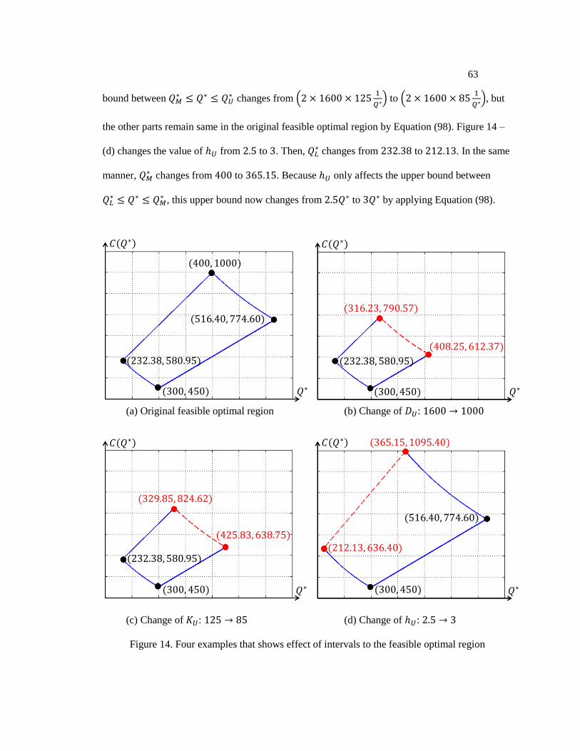
63
bound between
changes from (
) to (
), but
the other parts remain same in the original feasible optimal region by Equation (98). Figure 14 –
(d) changes the value of from to . Then, changes from to . In the same
manner, changes from to . Because only affects the upper bound between
, this upper bound now changes from to by applying Equation (98).
(a) Original feasible optimal region (b) Change of :
(c) Change of : (d) Change of :
Figure 14. Four examples that shows effect of intervals to the feasible optimal region

64
5.2 A Numerical Example for Minimax Analysis of the Basic EOQ Model
Now in this section, we are going to have the numerical example which shows how to
find the optimal order quantities at which the worst error is minimized by using both the worst
error ratio and the worst error difference, respectively. Based on Figure 13 which describes the
feasible optimal region under the intervals of D, K, and h, one can predict how the minimum
average cost could change and what would be the highest minimum average cost and the lowest
minimum average cost at which economic order quantities, respectively. For instance, when the
intervals of D, K, and h follow Intervals (95), the lowest minimum average cost is 450 at the
economic order quantity of 300, and the highest minimum average cost is 1000 at the economic
order quantity of 450. This implies that a manager will obtain the lowest minimum average cost
of 450 in the whole feasible optimal region if he successfully controls the values of D, K, and h.
The problem is, however, it is almost impossible to control D, K, and h to have the exact values a
manager wants. This is because these values are the costs easily affected and changed by the
diverse economic factors. Besides, even though a manager tries to control D, K, and h to have the
exact values a manager wants, the controlled values could be changed again. Therefore, the
estimated values of D, K, and h could be different from their true values. We call it error. For
example, by using Figure 13, a manager found that the minimum average cost is set to shrink by
up to 450 at , and , thus he controlled D, K, and h to have these value.
By using Equation (3), the economic order quantity at , and is 300. But
what if the values of D and K are affected and changed by some economic factors in spite of his
effort to keep their values? That is, true values of D and K are 1600 and 125, although a true
value of h is same as its estimate of 1.5. Then, by using Equation (1), the average cost at
, , and is
65
( )
(100)
and by using Equation (4), the minimum average cost at , and is
√ (101)
Therefore, the percentage of additional cost by selecting wrong approximates is
( )
(102)
From the result of equation (102), we can conclude that the error caused by selecting the wrong
approximates of D, K, and h incurs the increase of cost by up to 15.11%. Similarly, the amount of
additional cost is
( ) (103)
Then, we can interpret the result of Equation (103) as the additional cost is 117.07 by the error.
The error would increase more in other situations, which implies that the percentage or the
amount of the additional cost would be even larger. That is why we want to find the worst error
and minimize it by two different views; a ratio and a difference between a feasible average cost
and the minimum average cost.
By using Equations (35) and (48), we can minimize two functions, ( ) and ( ),
which are the worst error ratio and the worst error difference, respectively, as
( ) {
( )
} (104)
( ) {
( ) } (105)
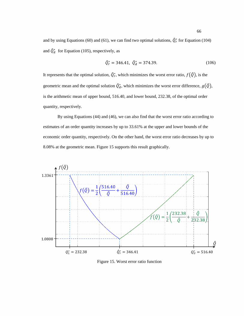
66
and by using Equations (60) and (61), we can find two optimal solutions, for Equation (104)
and for Equation (105), respectively, as
,
(106)
It represents that the optimal solution, , which minimizes the worst error ratio, ( ), is the
geometric mean and the optimal solution , which minimizes the worst error difference, ( ),
is the arithmetic mean of upper bound, 516.40, and lower bound, 232.38, of the optimal order
quantity, respectively.
By using Equations (44) and (46), we can also find that the worst error ratio according to
estimates of an order quantity increases by up to 33.61% at the upper and lower bounds of the
economic order quantity, respectively. On the other hand, the worst error ratio decreases by up to
8.08% at the geometric mean. Figure 15 supports this result graphically.
Figure 15. Worst error ratio function
( )

67
Similarly, by using Equations (56) and (58), the worst error difference has its maximum
of 433.92 at lower bound of the economic order quantity, and it has minimum of 67.33 at the
arithmetic mean of the maximum and the minimum EOQ’s. Figure 16 summarizes this result.
Figure 16. Worst error difference function
One of the interesting results is that is a little greater than
.
When all the numbers are positive, it is obvious that the arithmetic mean, , is always greater
than the geometric mean, , unless lower bound is equal to upper bound of the order quantity.
From our standpoint, if goods are turned out on a mass production basis, the setup cost and the
demand rate are generally much higher, but the inventory holding cost is relatively lower than
other costs. Thus in this case, we recommend that , can be a better solution than
to minimize the worst error because we can hold numerous amounts of inventories
by low inventory holding cost and also because we can decrease the number of orders which
( )

68
causes high setup cost. On the other hand, if goods are turned out on a diversified small-quantity
production basis, e.g., luxury items, the setup cost and the demand rate are generally lower, but
the inventory holding cost is relatively higher than other costs. Thus in that situation, we had
better decrease the high inventory holding cost by ordering and increasing the order
frequency. In this example, however, the difference between and
is not relatively big.
Therefore, selecting any of those solutions leads a similar result. On the contrary to this example,
if the difference between the upper and lower bounds goes to larger, the difference between
and is also going to be larger, and it should be paid close attention to selecting the suitable
solution either or
.
5.3 A Numerical Example for Robust Analysis of the Deterministic Serial Two-
Echelon Inventory Model
Now in this section, we extend our numerical example to robust analysis of the
deterministic serial two-echelon inventory model. Similar to the previous two numerical
examples, we do not have specific information about the exact values of the parameters that
compose the inventory model since it is hard to estimate their exact values in real life inventory
problem, except the multiplicity factor . As mentioned in Section 4.3, we first assume that the
multiplicity factor is fixed by contract and a manager knows this value. Thus in this numerical
example, we only know the fixed multiplicity factor , and we predict rough intervals of the other
parameters as
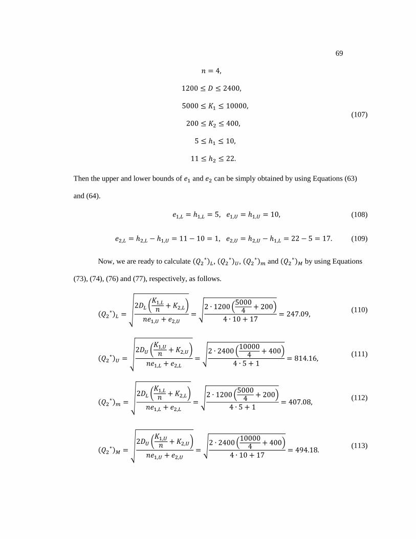
69
(107)
Then the upper and lower bounds of and can be simply obtained by using Equations (63)
and (64).
, (108)
, (109)
Now, we are ready to calculate ,
, and
by using Equations
(73), (74), (76) and (77), respectively, as follows.
√ (
)
√ (
)
(110)
√
(
)
√ (
)
(111)
√
(
)
√ ( )
(112)
√
(
)
√ (
)
(113)
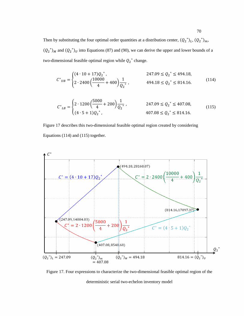
70
Then by substituting the four optimal order quantities at a distribution center, ,
,
and
into Equations (87) and (90), we can derive the upper and lower bounds of a
two-dimensional feasible optimal region while change.
{
(
)
(114)
{
(
)
(115)
Figure 17 describes this two-dimensional feasible optimal region created by considering
Equations (114) and (115) together.
Figure 17. Four expressions to characterize the two-dimensional feasible optimal region of the
deterministic serial two-echelon inventory model

71
Figure 17, however, cannot be a final version of the feasible optimal region we want because it is
hard to know directly how affects . Thus, the final feasible optimal region should be
described both in terms of and
. To reflect the power of to the feasible optimal
region, we use Equation (17), that is,
(116)
Also, by using Equations (91) and (92), we can infer and
as
(117)
(118)
Within the interval of derived by Equations (117) and (118), now we can make it three-
dimensional by adding Equation (116) to Figure 17. This three-dimensional feasible optimal
region is meaningful in the way that it shows how and
interact on each other and have an
influence on . Figure 18 represents the three-dimensional feasible optimal region of this
numerical example.

72
Figure 18. Extension of the two-dimensional feasible optimal region to the three-dimensional
feasible optimal region
In addition, we want to analyze how the multiplicity factor in Equation (6) affects the
area of the feasible optimal region. In Section 4.3, we found that the interval of decreases as
goes to large, and it finally implies a decrease in area of the feasible optimal region. To
simplify our analysis about area, we only consider the integral in terms of . Then the area of
the feasible optimal region can be calculated as
∫ ( )
∫ (
)
∫ (
)
∫ ( )
(119)
In this numerical example, . Thus, the area of the feasible optimal region of this example is

73
∫
∫ (
)
∫ (
)
∫
(120)
Table 1 summarizes the areas of the feasible optimal region when the multiplicity factor
changes and the other parameters keep same intervals.
Table 1. Area of the feasible optimal region according to the multiplicity factor
1 28,156,328.87
2 11,790,580.06
3 7,241,195.67
4 5,212,320.49
5 4,089,295.07
6 3,384,523.77
7 2,904,320.96
8 2,557,582.57
9 2,296,189.83
10 2,092,477.72
Based on the results in Table 1, Figure 19 shows the area of the feasible optimal region decreases
logarithmically as goes to large.

74
Figure 19. Logarithmically decreasing relationship between the multiplicity factor and the area of
the feasible optimal region
Under input data uncertainty, the feasible optimal region represents all the possible optimal
solution sets by different combinations of the input data in their intervals. Thus, a decrease in area
of the feasible optimal region represents a decrease in variability. Considering that a manager can
control the multiplicity factor by making or renewing contract, Figure 19 implies that he can
make risk management by increasing the multiplicity factor even if he fails to control the other
parameters that compose the deterministic serial two-echelon inventory model. However, it is
impossible to increase to the infinity in the real world. Therefore, increasing at its practical
level is the key to success on risk management under uncertainty of the parameters.
Table 1 and Figure 19 stimulate our curiosity about the relationship between the
multiplicity factor and the minimum total cost . Thus, now we release the assumption that the
multiplicity factor is fixed. Instead, a manager can analyze the minimum total cost with various
Area of the feasible optimal region
75
multiplicity factors until next contract, then he selects the best multiplicity factor for the
minimum total cost when he renews contract. To do this, we are going to use the method
developed in Section 4.3 to this numerical example and consider the effect of the number of
multiplicity factor to the feasible optimal region. The first step is to find the interval of the
optimal multiplicity factor, , by using Interval (94), that is,
√
√
√
√
(121)
Since the multiplicity factor should be positive integer, the set is {2, 3, 4, 5, 6, 7, 8, 9, 10, 11,
12, 13}. Now for each positive integer , we investigate the feasible optimal region. Table 2
summarizes the main EOQ values, such as ,
, ,
, and lower and upper
bounds, such as and , for each positive integer in Interval (121). Figure 20 describes
all the feasible optimal regions according to different multiplicity factors. Since we have twelve
different multiplicity factors, Figure 20 has twelve different feasible optimal regions of the
minimum total cost. As observed in Figure 19 and Table 1, Figure 20 graphically shows that the
area of the feasible optimal region becomes smaller as goes to large. Since the area of the
feasible optimal region implies the cost variability under input data uncertainty, we can have
smaller variability by increasing the value of . For example, the area of the feasible optimal
region in the numerical example is 11,790,580.06 when is 2. But the area is now at less than
half the area at = 2 when goes to 4. A manager can control the multiplicity factor when
renewing contract, thus controlling the value of can be a sure method to decrease the cost
variability under input data uncertainty. However, there is one problem with increasing the value

76
of . As seen in Table 2 and Figure 20, increasing the value of also generally causes increase
in lower and upper bounds of the minimum total cost. Therefore, we should be careful to pick the
value of at which the minimum total cost is minimized with small variability.
Table 2. Summary of the main values according to the multiplicity factor
2 418.49 767.52 836.98 1,535.05 8,442.75 30,968.37 11,790,580.06
3 308.74 529.15 617.48 1,058.30 8,466.40 29,021.37 7,241,195.67
4 247.09 407.08 494.18 814.16 8,548.68 28,168.07 5,212,320.49
5 207.33 332.82 414.66 665.64 8,653.32 27,782.01 4,089,295.07
6 179.47 282.84 358.93 565.69 8,768.12 27,637.66 3,384,523.77
7 158.81 246.89 317.63 493.77 8,887.87 27,633.52 2,904,320.96
8 142.87 219.76 285.74 439.51 9,009.99 27,717.14 2,557,582.57
9 130.18 198.55 260.36 397.09 9,133.09 27,858.69 2,296,189.83
10 119.83 181.50 239.66 362.99 9,256.35 28,039.97 2,092,477.72
11 111.22 167.49 222.44 334.97 9,379.28 28,249.28 1,929,473.95
12 103.94 155.76 207.87 311.53 9,501.58 28,478.76 1,796,217.68
13 097.70 145.80 195.39 291.61 9,623.05 28,722.97 1,685,329.37

77
Figure 20. Twelve different two-dimensional feasible optimal regions of the deterministic serial
two-echelon system according to the multiplicity factor
The one interesting observation is that the trace of describes an increasing
parabola, while the trace of increases steadily as goes to large. Figure 21 shows
function and function graphically. Since the increment of is relatively larger than
that of , we focus more on . Note that the value of has its minimum at
and second minimum at in this example. Actually, the value of at is almost
equal to the value of at , but the value of at is 119.75 even smaller
than the value of at . Thus, someone would select for its best option. Our
standpoint, however, also consider the area of the feasible optimal region. The area is 480202.81
smaller at than the area at . The smaller area implies the smaller variability of the
=5
=2
=8
=11 =12
=9
=6
=3 =4
=7
=10
=13

78
total minimum cost. Besides, the difference between the areas at and at is too huge
to ignore. Therefore, in this numerical example we recommend that the manager selects as
the best multiplicity factor to minimize upper bound of the minimum total cost, , with
appropriate variability when he renews contract.
Figure 21. Change of the upper and lower bounds of the minimum total cost of the deterministic
serial two-echelon inventory model

79
Chapter 6
CONCLUSION
6.1 Summary of the Thesis
This thesis considered robust analysis of the basic EOQ model and the deterministic
serial two-echelon inventory model by developing the closed form expressions that characterize
the set of all possible EOQ’s and corresponding minimum average costs. This thesis also
provided a method to reduce randomness in the worst case scenario. Since the parameters are
generally unknown and sometimes it is also hard to identify information about their probability
distributions in real life inventory problem, this thesis describes uncertainty of each parameter as
a continuous value that is restricted to some prespecified interval, from a robust optimization
point of view (Rosenhead et al. 1972).
First of all, we studied the basic EOQ model from a robust analysis point of view. The
basic EOQ model consists of three parameters; demand per unit time (D), ordering cost (K), and
inventory holding cost per unit per unit time (h). Since all these parameters are unknown,
combinations of different values of these parameters often lead to the same EOQ with different
minimum average costs. By considering this situation, we derived expressions for the upper and
lower bounds of the minimum average cost for each EOQ. Then by considering the upper and
lower bounds together, we developed the closed form expressions that characterize the set of all
possible EOQs and corresponding minimum average costs. Since this set predicts possible
inventory situations, we regard this set as variability of the minimum average cost of the basic
EOQ model when all the parameters are unknown.

80
Secondly, we analyzed the effect of randomness in the worst case scenario of the basic
EOQ model, and then we suggested the closed form optimal order policy to minimize the worst
error. For this analysis, we considered two minimax approaches – the ratio approach and the
difference approach. The ratio approach defines the error as a ratio of a feasible average cost to
the minimum average cost, which is shown in Equation (35). On the other hand, the difference
approach defines the error as a difference between a feasible average cost and the minimum
average cost, shown in Equation (48). Thus, we can say that the concept of the ratio approach is
same to the concept of difference approach in the way that they both find and make the worst
error minimize. However, the definition of the error is mathematically different between the ratio
approach and the difference approach. As a result, the ratio approach and the difference approach
have different worst errors, and they suggest different optimal solutions to minimize the worst
error. In the ratio approach, the optimal solution to minimize the worst error becomes the
geometric mean of the maximum and the minimum EOQ’s. But the difference approach suggests
that the optimal solution becomes the arithmetic mean of the maximum and the minimum EOQ’s.
Note that the arithmetic mean is always greater than the geometric mean if numbers are positive
or if upper bound is not equal to lower bound. Thus, there are two possible options on selecting
an optimal order quantity to minimize the worst error between the arithmetic mean and the
geometric mean. If items are produced on a diversified small-quantity production basis, such as
luxurious items, we recommend the geometric mean as the optimal solution to minimize the
worst error. This is because a diversified small-quantity production basis generally has small
demand rate, and its ordering cost is relatively lower than inventory holding cost. Thus in order to
reduce the expensive inventory holding cost, we can frequently order small amounts (i.e., the
geometric mean of the maximum and the minimum EOQ’s) with a cheap ordering cost whenever
we need them to meet small demands. On the other hand, if items are produced on a mass
production basis, such as industrial products or manufactured goods, then the arithmetic mean is a

81
more appropriate solution to minimize the worst error. This is because a mass production basis
generally has high demand, and its ordering cost is relatively higher than the inventory holding
cost. Thus, we could reduce the expensive ordering cost by having a bulk order (i.e., the
arithmetic mean of the maximum and the minimum EOQ’s). Besides we can expect quantity
discounts for a large purchase.
Lastly, we performed robust analysis of the deterministic serial two-echelon inventory
model, and suggested a method that finds the best multiplicity factor to minimize upper bound of
the minimum total cost. In order to do that, we extended our closed form expressions from robust
analysis of the basic EOQ model, and characterized the set of all possible optimal order quantities
and corresponding minimum total costs for fixed multiplicity factor. However, multiplicity factor
can take different positive integer values. Thus, we calculated all possible multiplicity factors.
Then each multiplicity factor, we repeated the process that characterizes the set of all possible
optimal order quantities and corresponding minimum total costs. One interesting observation is
that the area of the feasible optimal region decreases logarithmically as the multiplicity factor
increases. Since the feasible optimal region consists of all the possible minimum total costs under
input data uncertainty, we can regard the feasible optimal region as the variability of the
minimum total cost in the two-echelon inventory model. Therefore, we can conclude that the
variability of the minimum total cost decreases logarithmically as the multiplicity factor
increases. It represents that an inventory manager can decrease variability of the minimum total
cost by increasing the multiplicity factor when making or renewing contract. This method is
simple and clear to decrease cost variability under input data uncertainty. But this method has one
problem: increasing the multiplicity factor sometimes causes increase in upper bound of the
minimum total cost even if it always reduces the cost variability logarithmically. To avoid this
problem, we introduced the simple method that finds the best multiplicity factor at which upper

82
bound of the minimum total cost is minimized with small cost variability. Table 3 summarizes
what we did in this thesis and main results.
Table 3. Summary of main results in this thesis
Section Field Methodology Main Results
Section
4.1
The Basic
EOQ Model
Robust Analysis
{
{
Section
4.2
The Basic
EOQ Model
Minimax
Analyses
Ratio
Approach
( )
{
(
)
√
(
) √
√
Difference
Approach
( )
{
{
}
{
}
Section
4.3
The
Deterministic
Serial Two-
Echelon
Inventory
Model
Robust Analysis
{
(
)
( )
{
( )
(
)

83
6.2 Contribution
This thesis derived the closed form expressions that characterize the set of all possible
EOQ’s and corresponding minimum average costs for the basic EOQ model, as well as the set of
all possible optimal order quantities and corresponding minimum total costs for the deterministic
serial two-echelon inventory model. Unfortunately, the parameters are unknown and changing
frequently in real life inventory problem (Gallego et al. 2001). Consequently, our closed form
expressions are capable of describing variability and predicting possible inventory situations
under input data uncertainty. For the basic EOQ model, we also provided the closed form
functions that analyze the effect of randomness in the worst case scenario by finding the optimal
order policy at which the worst error is minimized. These functions would be useful for risk-
averse management. When considering the two-echelon inventory model, we verified that an
inventory manager will decrease the variability of the minimum total cost if he/she increases the
multiplicity factor. This method is simple for decreasing the variability. The results of this thesis
are closed form, thus we can directly apply these results without needing to convert them into
each problem.
6.3 Future Research
In this thesis, we limited our robust analysis up to the deterministic serial two-echelon
inventory model with one manufacturer and one distribution center, but the real world has more
complex system. For example, the multiple-echelon inventory system with multiple
manufacturers, multiple distribution centers, multiple retailers, and multiple buyers. Thus, this
study can be extended to the robust analysis of the general multi-echelon inventory system.
84
REFERENCES
Anupindi, R., T. E. Morton, D. Pentico. 1996. The nonstationary stochastic lead-time inventory
problem: Near-myopic bounds, heuristics, and testing. Management Science 42(1): 124–
129.
Axsäter, S. 2000. Exact analysis of continuous review (R,Q) policies in two-echelon inventory
systems with compound poisson demand. Operations Research 48(5): 686–696.
Axsäter, S., W.-F. Zhang. 1999. A joint replenishment policy for multi-echelon inventory control.
International Journal of Production Economics 59(1-3): 243–250.
Tuesday Barter Report. 2000. $350 Billion Product Overstock & Surplus Inventory. Barter News.
Available at http://www.barternews.com/archive/01-04-00.htm (accessed date September
26, 2013)
Clark, A. J., H. Scarf. 1960. Optimal policies for a multi-echelon inventory problem.
Management Science 6(4): 475–490.
Dem’yanov, V. F., V. N. Malozemov. 1990. Introduction to Minimax. Dover Publications, New
York.
Diks, E. B., A. G. de Kok. 1998. Optimal control of a divergent multi-echelon inventory system.
European Journal of Operational Research 111(1): 75–97.
Dobson, G. 1988. Sensitivity of the EOQ model to parameter estimates. Operations Research
36(4): 570–574.
Erkip, N., W. H. Hausman, S. Nahmias. 1990. Optimal centralized ordering policies in multi-
echelon inventory systems with correlated demands. Management Science 36(3): 381–
392.
Federgruen, A., P. Zipkin. 1984. Approximations of dynamic, multilocation production and
inventory problems. Management Science 30(1): 69–84.
Gallego, G. 1998. New bounds and heuristics for (Q, r) policies. Management Science 44(2):
219–233.
Gallego, G., I. Moon. 1993. The distribution free newsboy problem: Review and extensions. The
Journal of the Operational Research Society 44(8): 825–834.
Gallego, G., J. K. Ryan, D. Simchi-Levi. 2001. Minimax analysis for finite-horizon inventory
models. Institute of Industrial Engineers Transactions 33(10): 861–874.
Glasserman, P., S. Tayur. 1995. Sensitivity analysis for base-stock levels in multiechelon

85
production-inventory systems. Management Science 41(2): 263–281.
Grossinho, M. R., S. A. Tersian. 2001. An introduction to minimax theorems and their
applications to differential equations. Kluwer Academic Publishers, Boston.
Harris, R. S. 1913. How many parts to make at once. Factory, The Magazine of Management
10(2): 135–136.
Hillier, F. S., G. J. Lieberman. 2010. Introduction to Operations Research. Hillier, F. S., G. J.
Lieberman, 9th ed. Deterministic Multiechelon Inventory Models for Supply Chain
Management. McGraw Hill, New York, 848–865.
Hopp, W. J., R. Q. Zhang, M. L. Spearman. 1999. An easily implementable hierarchical heuristic
for a two-echelon spare parts distribution system. Institute of Industrial Engineers
Transactions 31(10): 977–988.
Iida, T. 2001. The infinite horizon non-stationary stochastic multi-echelon inventory problem and
near-myopic policies. European Journal of Operational Research 134(3): 525–539.
Karlin, S. 1960. Dynamic inventory policy with varying stochastic demands. Management
Science 6(3): 231–258.
Kasugai, H., T. Kasegai. 1960. Characteristics of dynamic maximin ordering policy. Journal of
the Operations Research Society of Japan 3: 11–26.
Kasugai, H., T. Kasegai. 1961. Note on minimax regret ordering policy – static and dynamic
solutions and a comparison to maximin policy. Journal of the Operations Research
Society of Japan 3: 155–169.
Langenhoff, L. J. G., W. H. M. Zijm. 1990. An analytical theory of multi-echelon
production/distribution systems. Statistica Neerlandica 44(3): 149–174.
Lin, Y.-J. 2008. Minimax distribution free procedure with backorder price discount. International
Journal of Production Economics 111(1): 118–128.
Lowe, T. J., L. B. Schwarz. 1983. Parameter estimation for the EOQ lot-size model: Minimax and
Expected Value Choices. Naval Research Logistics Quarterly 30(2): 367–376.
Moon, I., S. Choi. 1997. Distribution free procedures for make-to-order (MTO), make-in-advance
(MIA), and composite policies. International Journal of Production Economics 48(1):
21–28.
Moon, I., G. Gallego. 1994. Distribution free procedures for some inventory models. The Journal
of the Operational Research Society 45(6): 651–658.
Morton, T. E. 1978. The nonstationary infinite horizon inventory problem. Management Science
24(14): 1474–1482.
Morton, T. E., D. W. Pentico. 1995. The finite horizon nonstationary stochastic inventory
problem: Near-myopic bounds, heuristics, testing. Management Science 41(2): 334–343.

86
O’Connor, C. 2013. Wal-Mart Vs. Amazon: World’s biggest e-commerce battle could boil down
to vegetables. Forbes. Available at http://www.forbes.com/sites/clareoconnor/2013/04/
23/wal-mart-vs-amazon-worlds-biggest-e-commerce-battle-could-boil-down-to-
vegetables/ (accessed date September 25, 2013)
Ouyang, L.-Y., J.-S. Yao. 2002. A minimax distribution free procedure for mixed inventory
model involving variable lead time with fuzzy demand. Computers & Operations
Research 29(5): 471–487.
Rau, H. M.-Y. Wu, H.-M. Wee. 2003. Integrated inventory model for deteriorating items under a
multi-echelon supply chain environment. International Journal of Production Economics
86(2): 155–168.
Ren, L. 2010. The robustness of the basic EOQ. International Business & Economics Research
Journal 9(12): 17–22.
Rosenhead, J., M. Elton, S. K. Gupta. 1972. Robustness and optimality as criteria for strategic
decisions. Operational Research Quarterly 23(4): 413–431.
Rosling, K. 1989. Optimal inventory policies for assembly systems under random demands.
Operations Research 37(4): 565–579.
Sana, S. S. 2011. Price-sensitive demand for perishable items – an EOQ model. Applied
Mathematics and Computation 217(13): 6248–6259.
Scarf, H. 1958. A min-max solution of an inventory problem. Arrow, K. J., eds. Studies in the
Mathematical Theory of Inventory and Production. Stanford University Press, Stanford,
CA, 201–209.
Schwarz, L. B. 2008. The Economic Order-Quantity (EOQ) model. International Series in
Operations Research & Management Science 115: 135–154.
Sherbrooke, C. C. 1968. Metric: A multi-echelon technique for recoverable item control.
Operations Research 16(1): 122–141.
Sion, M. 1958. On general minimax theorems. Pacific Journal of Mathematics 8(1) : 171–176.
Snyder, L. V. 2006. Facility location under uncertainty: A review. Institute of Industrial
Engineers Transactions 38(7): 547–564.
Tee, Y.-S., M. D. Rossetti. 2002. A robustness study of a multi-echelon inventory model via
simulation. International Journal of Production Economics 80(3): 265–277.
Tsai, S. C., Y.-X. Zheng. 2013. A simulation optimization approach for a two-echelon inventory
system with service level constraints. European Journal of Operational Research 229(2):
364–374.
Van der Heijden, M. C., E. B. Diks, A. G. de Kok. 1997. Stock allocation in general multi-
echelon distribution systems with (R, S) order-up-to-policies. International Journal of
Production Economics 49(2): 157–174.

87
Walmart. 2013. 2012 Walmart Annual Report. Walmart. Available at http://www.walmartstores.
com/sites/annual-report/2012/WalMart_AR.pdf (accessed date September 26, 2013)
Yang, M-F., Y. Lin. 2010. Applying the linear particle swarm optimization to a serial multi-
echelon inventory model. Expert Systems with Applications 37(3): 2599–2608.
Yarow, J. 2012. Amazon was selling 306 items every second at its peak this year. Business
Insider. Available at http://www.businessinsider.com/amazon-holiday-facts-2012-
12#ixzz2fwGqO98A (accessed date September 25, 2013)
Yu, G. 1997. Robust economic order quantity models. European Journal of Operational
Research 100(3): 482–493.
Zhou, W.-Q., L. Chen, H.-M. Ge. 2013. A multi-product multi-echelon inventory control model
with joint replenishment strategy. Applied Mathematical Modelling 37(4): 2039–2050.