robust processing of magnetotelluric data in the amt dead band

Rd

X

sg8e

i

©

GEOPHYSICS, VOL. 73, NO. 6 NOVEMBER-DECEMBER 2008; P. F223–F234, 11 FIGS., 1 TABLE.10.1190/1.2987375

obust processing of magnetotelluric data in the AMTead band using the continuous wavelet transform

avier Garcia1 and Alan G. Jones2

dvgoagad

lnctnamcm

osblmTtmmi

edvc

ed 5Apsently I

dias.ie.

ABSTRACT

The energy sources for magnetotellurics MT at frequen-cies above 8 Hz are electromagnetic waves generated by dis-tant lightning storms propagating globally within the earth-ionosphere waveguide. The nature of the sources and proper-ties of this waveguide display diurnal and seasonal variationsthat can cause significant signal amplitude attenuation, espe-cially at 1–5 kHz frequencies — the so-called audiomagne-totelluric AMT dead band. This lack of energy results in un-reliable MT response estimates; and, given that in crystallineenvironments ore bodies located at some 500–1000-m depthare sensed initially by AMT data within the dead band, thisleads to poor inherent geometric resolution of target struc-tures. We propose a new time-series processing techniquethat uses localization properties of the wavelet transform toselect the most energetic events. Subsequently, two coher-ence thresholds and a series of robust weights are implement-ed to obtain the most reliable MT response estimates. Finally,errors are estimated using a nonparametric jackknife algo-rithm. We applied this algorithm to AMT data collected innorthern Canada. These data were processed previously us-ing traditional robust algorithms and using a telluric-telluricmagnetotelluric TTMT technique. The results show a sig-nificant improvement in estimates for the AMT dead bandand permit their quantitative interpretation.

INTRODUCTION

Time-varying, natural-source electromagnetic EM waves ob-ervable on the earth’s surface at frequencies above about 8 Hz areenerated by distant lightning activity and, at frequencies belowHz, by the interaction of the earth’s magnetosphere with particles

jected by the sun solar plasma. The former are important for au-

Manuscript received by the Editor 27 July 2007; revised manuscript receiv1Formerly Dublin Institute for Advanced Studies, Dublin, Ireland; pre

cm.csic.es.2Dublin Institute forAdvanced Studies, Dublin, Ireland. E-mail: [email protected] Society of Exploration Geophysicists.All rights reserved.

F223

iomagnetotelluric AMT studies of upper crustal structures for en-ironmental, energy, and resource exploration purposes, such asroundwater contamination, geothermal exploration, and discoveryf economic mineralization. Lightning-induced waves propagateround the globe in the electrically charged earth-ionosphere wave-uide Thomson, 1860; Wilson, 1920, and they penetrate the earthnd respond in amplitude and phase to the subsurface electrical con-uctivity structure.

Properties of the waveguide and the frequency characteristics ofightning display diurnal and seasonal variations that can cause sig-ificant signal amplitude variations, especially in the 1–5 kHz so-alled AMT dead band. These variations show an increase in ampli-ude during the summer months in the northern hemisphere and atighttime, and a corresponding decrease during the winter monthsnd daytime. Thus, one problem associated with applying the AMTethod for shallow 3km exploration can be the lack of signal in

ertain frequency bands during the desired acquisition interval. Forore information on AMT source analysis, see Garcia and Jones

2002.Traditional processing of MT data was based on approximations

f the least-squares method and assumptions of an ergodic, Gaussiantatistical model Bendat and Piersol, 1971; Sims et al., 1971, andoth are sensitive to small amounts of anomalous data and uncorre-ated noise. The inadequacy of the statistical model can cause the

agnetotelluric MT tensor to be strongly biased and unusable.hese biases were discussed first in MT by Sims et al. 1971; but

hey were known in other fields much earlier, particularly in econo-etrics Gini, 1921, and were discussed in Reiersøl 1950. The re-ote reference RR method Gamble et al., 1979 was developed to

ntroduce bias control in MT data processing.The first use of such an unbiased estimator for transfer function

stimation again comes from econometrics Reiersøl, 1941, and in-ependently from Geary 1943; see Reiersøl 1950 and Akaike1967, in which remote reference fields were termed instrumentalariables. The RR method consists of simultaneous recording typi-ally the horizontal magnetic fields measured at a second site that is

ril 2008; published online 5 November 2008.nstitut de Ciéncies del Mar, CSIC, Barcelona, Spain. E-mail: xgarcia@

scsriat

lbc21

aeaLciprbcbe

tfft

tlbJcaje1

lAstt5sf2otcd

ctawwtel

ndnoame

ttlnaejo

GtipM

tpcbhwafa

p

wFd

F224 Garcia and Jones

ufficiently remote from the main site so that noise sources are un-orrelated between the sites. Given the correct assumption that noiseources at both locations are uncorrelated, this method is effective inemoving the bias caused by uncorrelated noise. However, there ex-st unusual noise sources complex natural sources or cultural noisend frequency bands MT and AMT dead bands, which can causehe RR method to fail.

Coherence-sorting methods also have been applied. Data fromow signal-to-noise-ratio frequency bands e.g., MT or AMT deadands have been treated with a presorting method to eliminate lowoherence segments Egbert and Livelybrooks, 1996; Smirnov,003, although the method is not always useful Chave and Jones,997.

The introduction of data-adaptive weighting schemes, sometimeslong with the RR method, have been shown to eliminate the influ-nce of outliers in electric fields Jones and Joedicke, 1984; Egbertnd Booker, 1986; Chave et al., 1987; Chave and Thomson, 1989;arsen, 1989. Jones et al. 1989, who compare different MT pro-essing schemes applied to the same data set, document the superior-ty of these robust processing methods. Schultz et al. 1993 inter-reted the contamination of data collected using a large electrode ar-ay 1km spans, with electrodes at the bottom of a large lakeCarty Lake in northern Ontario, Canada, as the result of auroraNorthern Lights. This interpretation led to the development of a ro-ust processing technique with a leverage control that could detectontaminated data in electric and magnetic fields. More recently, Eg-ert and Livelybrooks 1996 and Chave and Thomson 2003, 2004xtended the removal of outliers to the magnetic fields.

Finally, Trad and Travassos 2000 introduce an approach usinghe wavelet transform. These authors use the discrete wavelet trans-orm DWT. A series of robust weights were applied to the trans-ormed data to remove noise. Subsequently, a robust processingechnique was applied to the antitransformed filtered data.

Another key component of processing, which indeed is as impor-ant as estimation of the response functions themselves, is the calcu-ation of their confidence limits. Least-squares impedance errorsased on Gaussian distributions typically are biased Chave andones, 1997 and unable to provide reliable uncertainty estimates. Inomparison, nonparametric methods are distribution independent;nd thus the error estimates are more accurate. The nonparametricackknife method of Richard von Mises see Efron, 1982 for errorstimation was introduced to MT processing by Chave and Thomson1989 and subsequently justified rigorously Thomson and Chave,991.

These estimation techniques, initially developed for processingong-period MT data, also have been applied to process AMT data.s mentioned previously, because of source characteristics the is-

ues related to problems in the AMT frequency band differ fromhose in the MT band; and these codes can fail to provide reliable es-imates of AMT transfer functions at frequencies of 1 kHz through

kHz. In particular, at high latitudes often there is little observableignal; and the few transients that are recorded must be located per-ectly in the time series, otherwise, the codes fail Garcia and Jones,002. Garcia and Jones 2005 introduce a new methodology basedn the use of electric transfer functions between sites and a base sta-ion, and on robust MT transfer functions from the base station re-orded at night, to solve the problem of lack of energy in the AMTead band at high latitudes.

For nonperiodic, nonstationary time series, the Fourier transforman give spurious results that have been solved to some extent withhe introduction of windowed Fourier transforms. As an alternativepproach, the wavelet transform might have advantages comparedith the Fourier transform for spectral analysis. Zhang and Paulson

1997 were the first to use wavelets, in their case the continuousavelet transform CWT, for processing AMT data. In their work,

he CWT is used to localize high-energy events. Then a new coher-nce thresholding technique, defined by the authors, permitted iso-ating bad data points.

This new coherence function assumes that the diagonal compo-ents of the impedance tensor are almost zero compared with the off-iagonal elements Zhang et al., 1997. For this reason, this tech-ique can fail in the presence of complicated three-dimensional ge-logy or galvanic distortions McNeice and Jones, 2001. The use ofstandard least-squares method to obtain the transfer functions alsoakes this technique sensitive to the presence of strong noise. Nev-

rtheless, the CWT has good localization properties.In this paper, we extend the work of Zhang and Paulson 1997

hat uses the CWT as a means to obtain spectra of the time series.Af-er calculating the wavelet spectra, the magnetic spectra are ana-yzed to locate the high-energy events. These can be either signal oroise, and for this reason we apply a coherence threshold methodnd a robust weighting technique to eliminate segments contaminat-d by uncorrelated noise. This method is completed with the use of aackknife nonparametric error-estimate technique for the calculationf confidence levels.

WAVELET TRANSFORM

In this section, we briefly describe the method of wavelet analysis.eneral bibliography on wavelets can be found in Daubechies

1990, Mallat 1998, and Percival and Walden 2000. A descrip-ion of the wavelet transform as applied to geophysics can be foundn Foufoula-Georgiou and Kumar 1995, and details about the ap-licability of wavelet analysis can be found in Weng and Lau 1994,eyers et al. 1993, and Torrence and Compo 1998.To analyze signal structures of very different sizes, it is necessary

o use time-frequency functions called atoms with varying time sup-orts an example of an atom would be the taper window used to cal-ulate the Fourier transform. The wavelet transform WT is capa-le of providing the time and frequency information simultaneously,ence giving a time-frequency representation of the signal. Theavelet transform is based on the two-parameter family of dilated

nd translated functions. Decomposing signals over this family ofunctions can be used to analyze time series that contain nonstation-ry power at many different frequencies Daubechies, 1990.

Let t be a fixed function mother wavelet, and consider a two-arameter family of dilated and translated functions; thus

b,s 1

s t b

s , 1

here s and b are the scale and translation parameters, respectively.unctions in the family obtained from equation 1 also are known asaughter functions. The term translation is used in the same sense as

iwoHFt

m

wmau

l

Tm1tm

wtle

Ewwct

lttC

w

tu

w

Ucn

tbeftfdt

m1wtdca

w

belc

Robust processing ofAMT data F225

n the windowed Fourier transform: It is related to the location of theindow as the window is shifted through the signal. This term obvi-usly corresponds to time information in the transform domain.owever, we do not have a frequency parameter, as we had for theourier transform. Instead, we have a scale parameter that is related

o the inverse of the frequency.To be admissible as a wavelet, a function must satisfy certainathematical criteria. First, a wavelet must have finite energy;

E

t2dt , 2

here E is the energy of a function equal to the integral of its squaredagnitude, and the vertical brackets represent the magnitude oper-

tor of . If t is a complex function, the magnitude must be foundsing its real and imaginary parts.

Second, considering f as the Fourier transform of t, the fol-owing condition must hold:

Cg 0

f2

fdf . 3

his implies that the wavelet has no zero-frequency component,ˆ 0 0; or, which is the same, the wavelet t must have a zero

ean. Equation 3 is known as the admissibility condition Farge,992, and Cg is called the admissibility constant. A third criterionhat applies to complex wavelets is that the Fourier transform of the

other wavelet must be real and vanish for negative frequencies.Given a time series, xn, with a time spacing t and n 0, . . . ,N1, the wavelet transform of x with respect to is defined as

Wg xb,s b,sx

dt1

s * t b

sxt , 4

b R, s 0,

here * indicates the complex conjugate. The continuous waveletransform of a discrete sequence xn similarly is defined as the convo-ution of xn with a discrete scaled and translated version of the moth-r wavelet 0h; thus

Wns n0

N1

xn · * n n t

s . 5

quation 5 measures the variation of x in the neighborhood of n,hose size is proportional to s. Mallat 1998, chap. 6 proves thathen the scale s goes to zero, the decay of the wavelet coefficients

haracterizes the regularity of x close to n; in other words, the lowerhe scale, the more localized the information that is obtained.

According to equation 5, to calculate the WT of a time series ofength N requires N convolutions. Given that in the Fourier domainhe N convolutions can be done simultaneously, the discrete Fourierransform DFT can be employed to speed up calculation of theWT Kaiser, 1994. The DFT of time series xn can be defined as

xk 1

Nn0

N1

xne2 ikn/N, 6

here k 0, . . . ,N 1 is the frequency index.Applying the convolution theorem, the wavelet transform equa-

ion 5 can be rewritten as the inverse Fourier transform of the prod-ct, or

Wns k0

N1

xk *skeikn t, 7

here the angular frequency k is defined as

k 2k

N t, k

N

2,

2k

N t, k

N

2. 8

sing equation 7 and a standard Fourier transform routine, the CWTan be calculated for a given scale s at all n data points simulta-eously and efficiently.

Because we are dealing with finite time series and using a Fourierransform that assumes these are cyclic, we have edge effects at theeginning and end of the wavelet power spectrum. The cone of influ-nce COI is the region of the wavelet spectrum in which edge ef-ects become important. In this work, we have followed the defini-ion of the COI by Torrence and Compo 1998 as the e-folding timeor the autocorrelation of wavelet power at each scale. The COI alsoefines at each scale the decorrelation time for a single spike in theime series.

The algorithm that we have developed accepts a choice of twoother wavelets, either the Morlet or the Paul Torrence and Compo,

998 wavelet. The one that we have found most successful in ourork is the Morlet wavelet Figure 1, and we restrict discussion in

his section to this type of function. The Morlet wavelet was intro-uced for geophysical exploration by Goupillaud et al. 1984; itonsists of a plane wave localized by a Gaussian function Grossmannd Morlet, 1987. Thus

0s 1/4ei0es2/2, 9

here 0 is the nondimensional frequency, in our work equal to2/log2.Strictly speaking, the Morlet wavelet, equation 9, is not a wavelet

ecause the admissibility condition, equation 3, does not hold. How-ver, if 0 0 is large enough; or, which is the same, if the scale s isarge enough, the negative frequency components of are smallompared with the progressive component Mallat, 1998; and this

sosldplm

wfcit

aipewts

Wltt

wcsdspdtn

eptlno

pTfbfTsse

cad

Ft


atisfies the admissibility condition. The parameter 0 allows trade-ff between time and frequency resolutions. The particular choice of0 in this work avoids problems with the Morlet wavelet at low

cales high temporal resolution, at the same time that it optimizesocalization properties of the wavelet in the temporal and spectralomains. Smaller values will improve the temporary localizationroperties while worsening the frequency localization, whereasarger values will emphasize the localization in the frequency do-

ain.The relationship between the equivalent Fourier period and the

avelet scale can be derived analytically for a particular waveletunction transforming a cosine wave of a known frequency, andomputing the scale s at which the wavelet power spectrum reachests maximum Torrence and Compo, 1998. For the Morlet wavelet,he Fourier period is expressed as

T 4s

0 2 0

. 10

Using equation 7, by varying the wavelet scale s and translatinglong the localized time index n, one can construct an image show-ng the amplitude of any features versus the scale and how this am-litude varies with time. We used this fact to localize high-energyvents better in the time series. To see the relationship between theavelet and Fourier spectra, the global wavelet spectrum must be in-

roduced. This is defined as the average of the wavelet spectra overcales,

W2s 1

Nn0

N1

Wns2. 11

hen smoothed, the Fourier spectrum approaches the global wave-et spectrum. Percival 1995 shows that the global wavelet spec-rum equation 11 provides an unbiased and consistent estimator ofhe true power spectrum of a time series.

−1

0

1

Am

plitu

de

−5 −4 −3 −2 −1 0 1 2 3 4 5

Time (s)

Morlet wavelet

Real

Imag

igure 1. Morlet wavelet. Left: Time representation of the Morlet mrum of the mother wavelet for four dilations see legend. Note that e

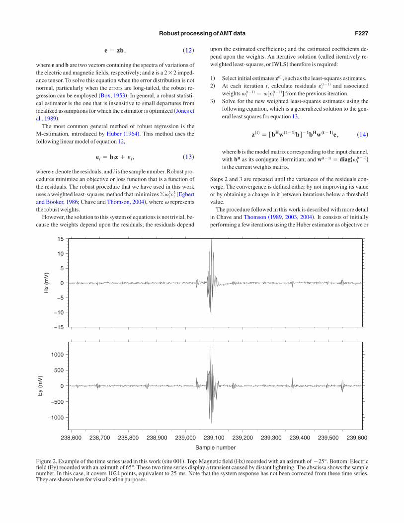
Figure 2 shows 1024 points 0.025 s of an electric field east-est component and the corresponding magnetic field north-south

omponent of some time series analyzed herein. This particularegment displays the arrival of a magnetotelluric transient caused byistant lightning. Figure 3 shows the wavelet spectrum for the timeeries in Figure 2. As can be observed, the spectrum has minimalower in the AMT dead band. The arrival of a transient caused byistant lightning enhances the energy in the AMT dead band, al-hough it still displays a minimum centered at 2000 Hz for the mag-etic field.

Localizing high-energy events can be the key to obtaining goodstimates in the dead-band, although there are two problems. Oneroblem is caused by lack of signal, even in presence of a transient;he other is caused by the presence of noise. To overcome the prob-em with noise, we propose the use of a robust remote reference tech-ique to downweight those noisy segments and allow for a selectionf clean high-energy events.

ROBUST PROCESSING

Jones and Joedicke 1984 propose a heuristic, jackknife robustrocessing method for MT data, based on maximizing coherence.his method later was modified to minimize variance and extended

or multiple remote references method 6 in Jones et al., 1989. Eg-ert and Booker 1986 and Chave and Thomson 1989 introducedormal, M-regression robust processing methods in MT. Chave andhomson 2004 extend the methods to allow for several referenceites. In this work, we consider a single reference site. The followingection focuses on the use of robust methods with one remote refer-nce site.

After the time series have been transformed into the time/frequen-y domain, the next step is to calculate the transfer functions. In thebsence of noise, the fundamental MT equation Dmitriev and Ber-ichevsky, 1979 can be expressed as

0

1

2

Am

plitu

de

10−1 100 101

Fourier frequency (Hz)

Spectrum of the Morlet wavelet

s = 20

s = 21

s = 22

s = 23

avelet for a time parameter 0 2/log2. Right: Fourier spec-ectrum has been scaled down by its corresponding scale factor.

other wach sp

wtangcia

Mf

wctuat

c

upw

12

3

Svov

ip

FfinT


e zb , 12

here e and b are two vectors containing the spectra of variations ofhe electric and magnetic fields, respectively; and z is a 22 imped-nce tensor. To solve this equation when the error distribution is notormal, particularly when the errors are long-tailed, the robust re-ression can be employed Box, 1953. In general, a robust statisti-al estimator is the one that is insensitive to small departures fromdealized assumptions for which the estimator is optimized Jones etl., 1989.

The most common general method of robust regression is the-estimation, introduced by Huber 1964. This method uses the

ollowing linear model of equation 12,

ei biz i, 13

here denote the residuals, and i is the sample number. Robust pro-edures minimize an objective or loss function that is a function ofhe residuals. The robust procedure that we have used in this workses a weighted least-squares method that minimizes i

2i2 Egbert

nd Booker, 1986; Chave and Thomson, 2004, where representshe robust weights.

However, the solution to this system of equations is not trivial, be-ause the weights depend upon the residuals; the residuals depend

−15

−10

−5

0

5

10

15

Hx

(mV

)

−1000

−500

0

500

1000

Ey

(mV

)

238,600 238,700 238,800 238,900 239,000

igure 2. Example of the time series used in this work site 001. Topeld Ey recorded with an azimuth of 65°. These two time series disumber. In this case, it covers 1024 points, equivalent to 25 ms. Nohey are shown here for visualization purposes.

pon the estimated coefficients; and the estimated coefficients de-end upon the weights. An iterative solution called iteratively re-eighted least-squares, or IWLS therefore is required:

Select initial estimates z0, such as the least-squares estimates. At each iteration t, calculate residuals i

t1 and associatedweights i

t1 it1 from the previous iteration.

Solve for the new weighted least-squares estimates using thefollowing equation, which is a generalized solution to the gen-eral least squares for equation 13,

zt bHwt1b1bHwt1e , 14

where b is the model matrix corresponding to the input channel,with bH as its conjugate Hermitian; and wt1 diagi

t1is the current weights matrix.

teps 2 and 3 are repeated until the variances of the residuals con-erge. The convergence is defined either by not improving its valuer by obtaining a change in it between iterations below a thresholdalue.

The procedure followed in this work is described with more detailn Chave and Thomson 1989, 2003, 2004. It consists of initiallyerforming a few iterations using the Huber estimator as objective or

,100 239,200 239,300 239,400 239,500 239,600

le number

etic field Hx recorded with an azimuth of 25°. Bottom: Electricransient caused by distant lightning. The abscissa shows the samplethe system response has not been corrected from these time series.

239

Samp

: Magnplay a tte that

ldtt

qsse

wfsfr

li

sbdnat

cjecto

as

Fbc


oss function. Then, using the more severe Thomson estimator, moreata are downweighted. Depending on data quality, this procedureakes only between three and eight iterations for each objective func-ion.

The remote reference method uses electromagnetic fields ac-uired at a distant location to minimize the local variance of the re-iduals. Following Chave and Thomson 1989, the weighted least-quares solution equivalent to equation 14 for a single remote refer-nce can be written

zt fRHwt1b1fR

Hwt1e , 15

here fR is the remote field used as a reference. The robust procedureor the remote reference case is the same as the one described in thisection. A more general form of the IWLS equation 14 can beound in Chave and Thomson 2004; it includes the use of severaleferences sites.

When the mean and variance of a set of independent and identical-y distributed data in the time domain are known, it is a simple task tonfer estimates of standard errors. However, it is common that data

3.0

3.5

4.0

log1

0(f

req

(Hz)

)

3.0

3.5

4.0

log1

0(f

req

(Hz)

)

238,600 238,700 238,800 238,900 239,000 239,10

Sample n

igure 3. Morlet wavelet transform of the time series used in Figure 2e seen that despite the arrival of a transient, the energy levels in theorrected in the spectra.

ets have mixed or very complicated e.g., multivariate error distri-utions; there are outliers, or an unknown number of degrees of free-om caused by correlation and heteroscedasticity. In such cases,onparametric methods are more appropriate to estimate the biasnd standard error in a statistic when a random sample of observa-ions is used to calculate it.

In this work, we have used the jackknife method to calculate theonfidence levels of the responses. The basic idea underpinning theackknife estimator lies in systematically recomputing the statisticstimate leaving out one observation at a time from the sample so-alled delete-one estimates. From this new set of observations forhe statistic, an estimate for the bias and an estimate for the variancef the statistic can be calculated Thomson and Chave, 1991.

Thomson and Chave 1991, among others, studied in detail thepplication of the jackknife method to the regression problem. Toolve the linear equation 14, a new set of pseudovalues can be usedHinkley, 1977, so that

zi z N1 hiz zi , 16

−3

−2

−1

0

1

log1

0(|

hx|)

nT

9,200 239,300 239,400 239,500 239,600−2

−1

0

1

2

3

log1

0(|

ey|)

mV/km

plots show the spectral and temporal structure of the transient. It canand 1–5 kHz remain low. Note that the system response has been

0 23

umber

. Thesedead b

wmtt

o

wt

w

mreo

mhirt

tctswmMatm

ptuctlwmacm

fi

teto

whe

ahfa

wi

tffctsTAi

iuastppse

tpt

Je


here z is the jackknifed estimate of the impedance z; z is an esti-ate of the impedance; zi is the estimate of the impedance based of

he ith subset the subset with the ith observation deleted; and hi ishe ith element of the diagonal of the hat matrix.

The hat matrix is a projection matrix from e into the column spacef z, defined as

H bbHb1bH, 17

here the superscript H denotes the Hermitian conjugate. Finally,he variance estimate of the impedance z can be determined using

varz 1

NN p i1

N

zi zzi zH, 18

here p is the number of columns in z.Diagonal elements of the hat matrix measure the distance of singleodel points from the center of the model, and the lack of balance is

eflected in their size. This allows for control of the leverage or influ-nce that elements of b have in the final estimate of z Chave and Th-mson, 2003.

ROBUST WAVELET PROCESSING ALGORITHM

The previous two sections briefly described the background infor-ation on the procedure followed in this work. The algorithm we

ave designed calculates wavelet spectra of the electric and magnet-c time series recorded at a site, and the reference fields recorded at aemote site. From those spectra, we derive MT response function es-imates using robust methods.

The reason for choosing a particular wavelet has to do with theype of problem to be explored. In magnetotellurics, the spectra arealculated to obtain the transfer functions; thus a complex, nonor-hogonal wavelet is appropriate. As the electromagnetic spectra aremoothly varying with frequency, the use of smooth, undulatingavelets is appropriate. The current algorithm allows use of twoother wavelets, either the Morlet or the Paul. In our experience, theorlet wavelet is better suited for magnetotellurics because it offersbetter trade-off between time and frequency resolution, whereas

he Paul wavelet has better localization properties in the time do-ain.After the wavelet spectra have been derived, the ensemble then is

urged of those segments for which the amplitude spectra are abouthe noise level of the magnetometers. This value can be set to the val-e provided by the instrument manufacturer. It has been shown Gar-ia and Jones, 2002 that in severe quiet times in theAMT dead band,he data recorded by the magnetometers correspond to their noiseevels. In addition, those segments located outside the COI of theavelet transform are purged also. To avoid rejecting too many seg-ents, and because computer memory is no longer an issue, we usu-

lly calculate the CWT of the whole time series; the alternative is tohop them into smaller sections, saving memory but sacrificing seg-ents at the edges.The next stage consists of the application of a series of coherence

lters to the spectra, which permits detection of uncorrelated sec-

ions. Two kinds of coherence functions are used, a classical coher-nce and a wavelet coherence. The classical thresholding techniquehat is applied initially to the spectra uses the auto and cross-spectraf the EM time series and can be defined as

2 Wab2

WaaWbb, 19

here · indicates smoothing in time. Those sections in which co-erence is below a specific threshold defined by the user are discard-d.

A wavelet coherence technique Torrence and Webster, 1999 ispplied. Whereas the classical coherence technique searches for co-erent segments along the temporal axis, the wavelet coherenceunction allows for a search for noncoherent segments across scalesnd time axes. The wavelet squared coherence function is defined as

wavelet2

s1Wab2

s1Waa2s1Wbb2, 20

here · indicates smoothing in both time and scale. The factor s1

s used to convert to an energy density.In general, low and high power segments are rejected, because

hey are susceptible to either not being coherent or being strongly af-ected overwhelmed by coherent noise. Lower and upper valuesor the threshold can be set in the algorithm. In some instances, noisean be correlated severely between the channels; and the upperhresholding permits eliminating some of this noise. This methodhould be used with care because it also can eliminate clean sections.he remaining segments are used for the final response calculation.t this point, the responses are calculated and will be used as a start-

ng estimate for the robust processing and as nonrobust estimates.The next step consists of calculation of the hat matrix for later use

n the jackknife calculation of confidence intervals. The hat matrix issed in statistics to identify high leverage points that are outliersmong the independent variables. The algorithm that we have de-igned allows one to set a thresholding level based on the diagonal ofhe hat matrix, although the tests that we have run suggest no im-rovement of the final responses. After this step, the robust iterationrocess step is initiated, and it downweights the remaining noisyegments. The final stage involves calculation of the confidence lev-ls using a jackknife procedure.

The algorithm is written in standard FORTRAN 95. Each of theime series used in this work consists of 262,144 points with a sam-le rate of 40,960 Hz 6.4 s in total time length; the total processingime is about two minutes on a Pentium PC.

EXAMPLE: THE NORMAN TOWNSHIP DATA SET

We applied the robust code that we present here to data acquired inuly 2000 in Norman Township Sudbury, Ontario, Canada. Thisxperiment was designed to test a new telluric-telluric magnetotellu-

rietntTq

vbtqpta

aSntu

ih4hfuf

Ts

FfoAtis located in UTM WGS84, zone 17.

FBsmaining after rejection by coherence thresholding.


ic methodology TTMT proposed by Garcia and Jones 2005, andnvolved acquiring four profiles of AMT data with a remote refer-nce site. The TTMT method consists of the use of electric-field day-ime measurements at all stations profile, base, and remote, andighttime measurements at the base and remote stations. Using theransfer functions between daytime and nighttime time series, aTMT response function can be calculated for measurements ac-uired during daytime.

In this work, we process data from the northern profile of the sur-ey Figure 4, and compare the resulting estimates with previousest estimates from robust, conventional MT processing. Becausehe experiment was designed to test the TTMT method, data were ac-uired at different times of the day. Table 1 summarizes site occu-ancy of data recorded on July 20, 2000. Unfortunately, for site 006he remote reference was not recording. We have used the only sitevailable at that time, 004, as a reference.

Processing consists of four fundamental steps. First, time seriesre transformed into the spectral domain using wavelet methods.econd, power and coherence thresholding is applied to eliminateoisy sections. Third, a robust, least-squares technique is used to ob-ain the impedances. Fourth, the confidence intervals are calculatedsing the nonparametric jackknife method.

Processing of data begins with the transform of the EM time seriesnto the wavelet domain. The data sets that we use in this exampleave 262,144 points and were acquired using a sampling rate of0,690 Hz. To avoid rejecting segments because of the COI, weave not split the time series into short segments, and thus, only aew data points at the beginning and end are affected. This operationsually takes 1 minute of computer time in a normal Pentium PCor six electromagnetic channels four locals and two remotes. At

the same time, deconvolution of the instrumentresponse is applied also; and scales are convertedto frequencies.

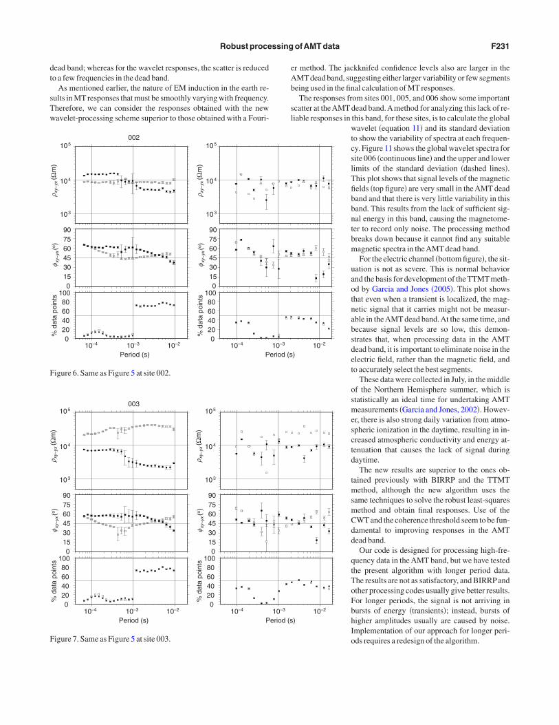
The second step consists of filtering data pointsusing coherence and wavelet coherence thresh-olding techniques. The amount of data that areeliminated depends on the values of thresholdinglimits set by the user and the quality of the data.Figures 5–10 show the MT responses of sites ana-lyzed in this study and a plot of percentage of dataleft after two-stage coherence thresholding. Thislater procedure eliminates, in most cases, morethan 90% of the data. For longer periods, we havefound that the coherence thresholding is not as ef-ficient as in the AMT dead band, and we usuallyrelax this thresholding; thus, the amount of dataeliminated is smaller. The data that are not elimi-nated by coherence thresholding are used in theimpedance tensor estimates of final responses us-ing the IWLS technique described previously.

On the left panels of Figures 5 through 10 arethe responses obtained from the code developedin this work; on the right are the responses ob-tained using a robust Fourier transform algorithmbounded influence, remote reference processing,BIRRP, Chave and Thomson, 2004, whichrepresent the best conventional MT responsesthat we could obtain. The Fourier responses showscatter at all frequencies, especially in the AMT

)10−2

T left andes and whitege of data re-

able 1. Table showing site occupancy (GMT-5:00 EST) forites used on July 20, 2000.

Site name occupancy local time, GMT-5:00 EST

RR 001 002 003 004 005 006

11:40 11:40

13:00 13:00 13:00

14:00 14:00

15:40 15:40

16:40 16:40

5179

5178

5177

Nor

thin

g(k

m)

496 497 498 499 500 501 502 503 504 505 506 507

Easting (km)

005006RR

004003002001

igure 4. Location of the northern profile with sites used in this workrom Norman Township experiment that tested a new TTMT meth-dology to acquire and process data to improve responses in theMT dead band. The site marked with a diamond indicates the loca-

ion of the remote reference site Garcia and Jones, 2005. This area

001510

ρ xy−

yx(Ω

m)

9075604530150

φ xy−

yx(o

)

100806040200

%da

tapo

ints

10−4

Period (s

410

310

10−310−4

Period (s)10−3 10−2

510

ρ xy−

yx(Ω

m)

9075604530150

φ xy−

yx(o

)

100806040200

%da

tapo

ints

410

310

igure 5. Apparent resistivities and phases at site 001 computed using CWIRRP right methods. Black symbols correspond to the zxy impedanc

ymbols to the zyx impedances. On the bottom panel is a plot of the percenta

dt

sTw

eAb

sl

F

F


ead band; whereas for the wavelet responses, the scatter is reducedo a few frequencies in the dead band.

As mentioned earlier, the nature of EM induction in the earth re-ults in MT responses that must be smoothly varying with frequency.herefore, we can consider the responses obtained with the newavelet-processing scheme superior to those obtained with a Fouri-

002

10−4

P10−4

Period (s)10−3 10−2

510

ρ xy−

yx(Ω

m)

9075604530150

φ xy−

yx(o

)

100806040200

%da

tapo

ints

410

310

510

ρ xy−

yx(Ω

m)

9075604530150

φ xy−

yx(o

)

100806040200

%da

tapo

ints

410

310

igure 6. Same as Figure 5 at site 002.

003510

ρ xy−

yx(Ω

m)

9075604530150

φ xy−

yx(o

)

100806040200

%da

tapo

ints

410

310

510

ρ xy−

yx(Ω

m)

9075604530150

φ xy−

yx(o

)

100806040200

%da

tapo

ints

410

310

10−4

Period (s)10−3 10−2 10−4

P


r method. The jackknifed confidence levels also are larger in theMT dead band, suggesting either larger variability or few segmentseing used in the final calculation of MT responses.

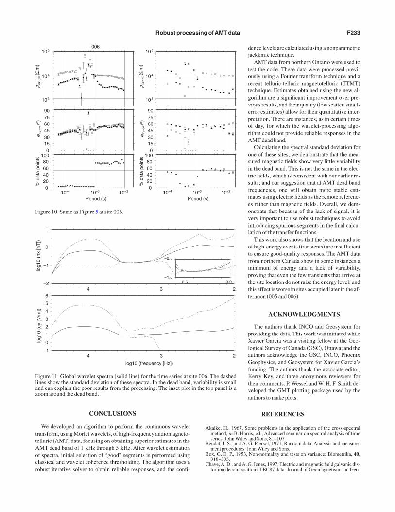
The responses from sites 001, 005, and 006 show some importantcatter at theAMT dead band.Amethod for analyzing this lack of re-iable responses in this band, for these sites, is to calculate the global

wavelet equation 11 and its standard deviationto show the variability of spectra at each frequen-cy. Figure 11 shows the global wavelet spectra forsite 006 continuous line and the upper and lowerlimits of the standard deviation dashed lines.This plot shows that signal levels of the magneticfields top figure are very small in the AMT deadband and that there is very little variability in thisband. This results from the lack of sufficient sig-nal energy in this band, causing the magnetome-ter to record only noise. The processing methodbreaks down because it cannot find any suitablemagnetic spectra in theAMT dead band.

For the electric channel bottom figure, the sit-uation is not as severe. This is normal behaviorand the basis for development of the TTMT meth-od by Garcia and Jones 2005. This plot showsthat even when a transient is localized, the mag-netic signal that it carries might not be measur-able in theAMT dead band.At the same time, andbecause signal levels are so low, this demon-strates that, when processing data in the AMTdead band, it is important to eliminate noise in theelectric field, rather than the magnetic field, andto accurately select the best segments.

These data were collected in July, in the middleof the Northern Hemisphere summer, which isstatistically an ideal time for undertaking AMTmeasurements Garcia and Jones, 2002. Howev-er, there is also strong daily variation from atmo-spheric ionization in the daytime, resulting in in-creased atmospheric conductivity and energy at-tenuation that causes the lack of signal duringdaytime.

The new results are superior to the ones ob-tained previously with BIRRP and the TTMTmethod, although the new algorithm uses thesame techniques to solve the robust least-squaresmethod and obtain final responses. Use of theCWT and the coherence threshold seem to be fun-damental to improving responses in the AMTdead band.

Our code is designed for processing high-fre-quency data in the AMT band, but we have testedthe present algorithm with longer period data.The results are not as satisfactory, and BIRRP andother processing codes usually give better results.For longer periods, the signal is not arriving inbursts of energy transients; instead, bursts ofhigher amplitudes usually are caused by noise.Implementation of our approach for longer peri-ods requires a redesign of the algorithm.

)10−2

)10−2

eriod (s10−3

eriod (s10−3

F

F


004410

ρ xy−

yx(Ω

m)

9075604530150

φ xy−

yx(o

)

100806040200

%da

tapo

ints

310

210

410

ρ xy−

yx(Ω

m)

9075604530150

φ xy−

yx(o

)100806040200

%da

tapo

ints

310

210

10−4

Period (s)10−3 10−2 10−4

Period (s)10−3 10−2


005510

ρ xy−

yx(Ω

m)

9075604530150

φ xy−

yx(o

)

100806040200

%da

tapo

ints

410

310

510

ρ xy−

yx(Ω

m)

9075604530150

φ xy−

yx(o

)

100806040200

%da

tapo

ints

410

310

10−4

Period (s)10−3 10−210−4

Period (s)10−3 10−2


ttAocr

A

B

B

C

F

Flaz


CONCLUSIONS

We developed an algorithm to perform the continuous waveletransform, using Morlet wavelets, of high-frequency audiomagneto-elluric AMT data, focusing on obtaining superior estimates in theMT dead band of 1 kHz through 5 kHz. After wavelet estimationf spectra, initial selection of “good” segments is performed usinglassical and wavelet coherence thresholding. The algorithm uses aobust iterative solver to obtain reliable responses, and the confi-

006510

ρ xy−

yx(Ω

m)

9075604530150

φ xy−

yx(o

)

100806040200

%da

tapo

ints

410

310

510

ρ xy−

yx(Ω

m)

9075604530150

φ xy−

yx(o

)

100806040200

%da

tapo

ints

410

310

10−4

Period (s)10−3 10−2 10−4

P


1

0

−1

−2

log1

0(h

x[n

T])

4 3

−1.0

−0.5

3.5

6

5

4

3

2

1

0

−1

log1

0(e

y[V

/m])

log10 (frequency [Hz])

4 3

igure 11. Global wavelet spectra solid line for the time series at sines show the standard deviation of these spectra. In the dead bandnd can explain the poor results from the processing. The inset plotoom around the dead band.

dence levels are calculated using a nonparametricjackknife technique.

AMT data from northern Ontario were used totest the code. These data were processed previ-ously using a Fourier transform technique and arecent telluric-telluric magnetotelluric TTMTtechnique. Estimates obtained using the new al-gorithm are a significant improvement over pre-vious results, and their quality low scatter, small-error estimates allow for their quantitative inter-pretation. There are instances, as in certain timesof day, for which the wavelet-processing algo-rithm could not provide reliable responses in theAMT dead band.

Calculating the spectral standard deviation forone of these sites, we demonstrate that the mea-sured magnetic fields show very little variabilityin the dead band. This is not the same in the elec-tric fields, which is consistent with our earlier re-sults; and our suggestion that at AMT dead bandfrequencies, one will obtain more stable esti-mates using electric fields as the remote referenc-es rather than magnetic fields. Overall, we dem-onstrate that because of the lack of signal, it isvery important to use robust techniques to avoidintroducing spurious segments in the final calcu-lation of the transfer functions.

This work also shows that the location and useof high-energy events transients are insufficientto ensure good-quality responses. The AMT datafrom northern Canada show in some instances aminimum of energy and a lack of variability,proving that even the few transients that arrive atthe site location do not raise the energy level; andthis effect is worse in sites occupied later in the af-ternoon 005 and 006.

ACKNOWLEDGMENTS

The authors thank INCO and Geosystem forproviding the data. This work was initiated whileXavier Garcia was a visiting fellow at the Geo-logical Survey of Canada GSC, Ottawa; and theauthors acknowledge the GSC, INCO, PhoenixGeophysics, and Geosystem for Xavier Garcia’sfunding. The authors thank the associate editor,Kerry Key, and three anonymous reviewers fortheir comments. P. Wessel and W. H. F. Smith de-veloped the GMT plotting package used by theauthors to make plots.

REFERENCES

kaike, H., 1967, Some problems in the application of the cross-spectralmethod, in B. Harris, ed., Advanced seminar on spectral analysis of timeseries: John Wiley and Sons, 81–107.

endat, J. S., and A. G. Piersol, 1971, Random data: Analysis and measure-ment procedures: John Wiley and Sons.

ox, G. E. P., 1953, Non-normality and tests on variance: Biometrika, 40,318–335.

have, A. D., and A. G. Jones, 1997, Electric and magnetic field galvanic dis-tortion decomposition of BC87 data: Journal of Geomagnetism and Geo-

)10−2

2

3.0

2

. The dashedility is small

top panel is a

eriod (s10−3

ite 006, variabin the

C

—

—

C

D

D

E

E

E

F

F

G

G

—

G

G

G

G

H

H

J

J

KL

MM

M

P

P

R

—

S

S

S

T

TT

T

T

W

W

Z

Z


electricity, 49, 4669–4682.have, A. D., and D. J. Thomson, 1989, Some comments on magnetotelluricresponse function estimation: Journal of Geophysical Research, 94,14215–14225.—–, 2003, Abounded influence regression estimator based on the statisticsof the hat matrix: Journal of the Royal Statistical Society, Series C Ap-plied Statistics, 52, 307–322.—–, 2004, Bounded influence estimation of magnetotelluric responsefunctions: Geophysical Journal International, 157, 988–1006.

have, A. D., D. J. Thomson, and M. E. Ander, 1987, On the robust estima-tion of power spectra, coherences, and transfer functions: Journal of Geo-physical Research, 92, 633–648.

aubechies, I., 1990, The wavelet transform, time-frequency localizationand signal analysis: IEEE Transactions on Information Theory, 36,961–1005.

mitriev, V. I., and M. N. Berdichevsky, 1979, The fundamental model ofmagnetotelluric sounding: Proceedings of the IEEE, 67, 1033–1044.

fron, B., 1982, The jackknife, the bootstrap, and other resampling plans:SIAM.

gbert, G. D., and J. Booker, 1986, Robust estimation of geomagnetic trans-fer functions: Geophysical Journal of the RoyalAstronomical Society, 87,173–194.

gbert, G. D., and D. Livelybrooks, 1996, Single station magnetotelluric im-pedance estimation: Coherence weighting and the regression M-estimate:Geophysics, 61, 964–970.

arge, M., 1992, Wavelet transforms and their applications to turbulence:Annual Review of Fluid Mechanics, 24, 395–457.

oufoula-Georgiou, E., and P. Kumar, 1995, Wavelets in geophysics: Aca-demic Press.

amble, T. D., W. M. Goubau, and J. Clarke, 1979, Magnetotellurics with aremote reference: Geophysics, 61, 53–68.

arcia, X., and A. G. Jones, 2002, Atmospheric sources for audio-magneto-telluric AMT sounding: Geophysics, 67, 448–458.—–, 2005, New methodology for the acquisition and processing of audio-magnetotelluric AMT data in the dead-band: Geophysics, 70, 119–126.

eary, R., 1943, Relations between statistics: The general and the samplingproblem when the samples are large: Proceedings of the Royal Irish Acad-emy, 49, 177–196.

ini, C., 1921, Sullâ interpolazione di una retta quando i valori della vari-abile indipendente sono affetti da errori accidentali: Metron, 1, 63–82.

oupillaud, P., A. Grossmann, and J. Morlet, 1984, Cycle-octave and relatedtransform in seismic signal analysis: Geoexploration, 33, 85–102.

rossman, A., and J. Morlet, 1987, Decomposition of hardy functions intosquare integrable wavelets of constant shape: SIAM Journal of Mathemat-icalAnalysis, 15, 723–736.

inkley, D. V., 1977, Jackknifing in unbalanced situations: Technometrics,19, 285–292.

uber, P., 1964, Robust estimation of a location parameter: Annals of Mathe-matical Statistics, 35, 73–101.

ones, A. G., A. D. Chave, G. Egbert, D. Auld, and K. Bahr, 1989, Acompar-ison of techniques for magnetotelluric response function estimation: Jour-nal of Geophysical Research, 94, 14201–14213.

ones, A. G., and H. Joedicke, 1984, Magnetotelluric transfer function esti-

mation improvement by a coherence-based rejection technique: 56th An-nual International Meeting, SEG, ExpandedAbstracts, 51–55.

aiser, G., 1994, Afriendly guide to wavelets: Birkhäuser.arsen, J. C., 1989, Transfer functions: Smooth robust estimates by leastsquares and remote reference methods: Geophysical Journal International,99, 655–663.allat, S., 1998, Awavelet tour of signal processing:Academic Press.cNeice, G. W., and A. G. Jones, 2001, Multisite, multifrequency tensor de-composition of magnetotelluric data: Geophysics, 66, 158–173.eyers, S. D., B. G. Kelly, and J. J. O’Brien, 1993, An introduction to wave-let analysis in oceanography and meteorology: With application to the dis-persion of Yanai waves: Monthly Weather Review, 121, 2858–2866.

ercival, D. B., 1995, On estimation of the wavelet variance: Biometrika, 82,619–631.

ercival, D. B., and A. T. Walden, 2000, Wavelet methods for time seriesanalysis: Cambridge University Press.

eiersøl, O., 1941, Confluence analysis by means of lag moments and othermethods of confluence analysis: Econometrica, 9, 1–22.—–, 1950, Identifiability of a linear relation between variables which aresubject to error: Econometrica, 18, 375–389.

chultz, A., R. D. Kurtz, A. D. Chave, and A. G. Jones, 1993, Conductivitydiscontinuities in the upper mantle beneath a stable craton: GeophysicalResearch Letters, 20, 2941–2944.

ims, W. E., F. X. Bostick, and H. W. Smith, 1971, The estimation of magne-totelluric impedance tensor elements from measured data: Geophysics,36, 938–942.

mirnov, M., 2003, Magnetotelluric data processing with a robust statisticalprocedure having a high breakdown point: Geophysical Journal Interna-tional, 152, 1–7.

homson, D. J., and A. D. Chave, 1991, Jackknifed error estimates for spec-tra, coherences, and transfer functions, in S. Haykin, ed., Advances inspectrum analysis and array processing, v. 1: Prentice Hall, 58–113.

homson, L. W., 1860, Electricity atmospheric: Nichols Cyclopedia.orrence, C., and G. P. Compo, 1998, A practical guide to wavelet analysis:Bulletin of theAmerican Meteorological Society, 79, 61–78.

orrence, C., and P. Webster, 1999, Interdecadal changes in the ENSO-mon-soon system: Journal of Climate, 12, 2679–2690.

rad, D. O., and J. M. Travassos, 2000, Wavelet filtering of magnetotelluricdata: Geophysics, 65, 482–491.eng, H., and K. M. Lau, 1994, Wavelets, period doubling, and time-fre-quency localization with application to organization of convection overthe tropical Western Pacific: Journal of Atmospheric Science, 51,2523–2541.ilson, C. T. R., 1920, Investigation on lightning discharges and on the elec-tric field of thunderstorms: Phylosophical Transactions of the Royal Soci-ety of London, SeriesA, 221, 73–115.

hang, Y., D. Goldak, and K. Paulson, 1997, Detection and processing oflightning-sourced magnetotelluric transients with the wavelet transform:IEICE Transactions on Fundamentals of Electronics, Communicationsand Computer Sciences, E80, 849–858.

hang, Y., and K. V. Paulson, 1997, Enhancement of signal-to-noise ratio innatural-source transient MT data with wavelet transform: Pure and Ap-
plied Geophysics, 149, 405–419.

robust processing of magnetotelluric data in the amt dead band

Documents