R ob u stn ess In S o lid M o d e lin g - A T o le ra n ce B ased , In tu it ion is t ic A p p ro a ch

Shiaofen Fang, Xiaohong Zhu, Beat Bruderlin

U U C S -9 2 -0 3 0

Department of Computer Science ' University of Utah •

Salt Lake City, UT 84112 USA

August 20, 1992

A b s t r a c tThis paper presents a new robustness method for geometric modeling operations. It com­

putes geometric relations from the tolerances defined for geometric objects and dynamically updates the tolerances to preserve the properties of the relations, using an intuitionistic self-validation approach. Geometric algorithms using this approach are proved to be ro­bust. A robust Boolean set operation algorithm using this robustness approach has been implementedand test examples are described in this paper as well.

R o b u s t n e s s I n S o l i d M o d e l i n g

— A T o l e r a n c e B a s e d , I n t u i t i o n i s t i c A p p r o a c h

Shiaofen Fang Beat Bruderlin Xiaohong Zhu

Computer Science Department

University of Utah ‘

Salt Lake City, UT 84112, USA

A b s t r a c t . This paper presents a new robustness method for geometric modeling

operations. It computes geometric relations from the tolerances defined for geometric objects

and dynamically updates the tolerances to preserve the properties of the relations, using an

intuitionistic self-validation approach. Geometric algorithms using this approach are proved

to be robust. A robust Boolean set operation algorithm using this robustness approach has

been implemented and test examples are described in this paper as well.

1 I n t r o d u c t i o n

1 .1 G e o m e t r i c R o b u s t n e s s P r o b l e m

Geometric algorithms are usually designed for objects defined over the domain of real num­

bers which can only be approximated on a computer, for instance, with floating point num­

bers. In addition to the floating point arithmetic errors, there often are geometric approxi­

mation errors, which are generated when only approximated solutions can be computed, e.

g. using a piecewise linear curve to approximate a higher degree curve.

Considering these errors, geometric algorithms are hardly robust without special treat­

ment. Computing relations between geometric objects (e.g. coincidence of points, colinear

lines or coplanar planes) using approximate numerical data is arbitrary and likely to be

inconsistent. This causes geometric algorithms to produce invalid geometric representations

Figure 1: (a) Computing the union of two objects; (b) Invalid result with dangling edge

or even crash.

An example is given in figure 1. A Boolean union operation is computed for two identical

cubes with one translated. The algorithm first finds that planes P and Q are coincident

within some defined tolerance. However, because of a slightly larger floating point error for

the representation of edge A B , the edge is found to be intersecting plane P instead of

being incident on plane P . Theoretically, if a line is incident on a plane Q, it is also incident

on all the planes that are coincident with Q. Algorithms based on such inconsistent decisions

produce an invalid solid representations like in figure 1(b), where a dangling edge is created.

More of these kinds of example can be found in [11],

1 .2 R e l a t e d W o r k

A number of publications have addressed the geometric robustness problem recently[12|[ll].

Approaches in [9] [24] [31] [32] perform precise computations by using only exact numbers (e.

g. bounded rational numbers, exact algebraic numbers or space grids). They work on the

supposition (that is often not true) that geometric shapes (and all computations on them)

can be represented with exact numbers. However, curves and curved surfaces are outside

the domain that can be represented by rational numbers. Approaches in [41 [34] perturb

the input data a small amount to avoid positional degeneracy. These approaches cannot

2

represent intentionally degenerate cases occurring in geometric modeling applications and

are therefore not suitable for CAD. Approaches in [14] [161 [19] [20] [211 [22] [29] [30] try to use

pure symbolic reasoning to maintain the consistency among all the decisions made regarding

geometric relations. However to strictly adhere to all the symbolic constraints necessitates

a theorem proving process[3][15][17] which is usually too complicated for practical applica­

tions. Provably fail-save symbolic inferencing is generally limited to some simple geometric

problems.

Tolerance-based approaches can be found in [1|[6][7][5|[28]. They keep sufficient informa­

tion about uncertainty regions (tolerances) of geometric objects and update the tolerances

according to the decisions made in order to maintain the consistency of the decisions. The

ideas of these approaches are partially derived from interval arithmetic[23]. A direct geo­

metric generalization of interval arithmetic is “Epsilon Geometry” [10] [27] [26]. A direct use

of dynamic tolerances can be found in a polyhedral Boolean operation algorithm developed

by Sega] [28], and [2]. In both approaches, geometric relations are detected based on the

tolerances of geometric objects. Tolerances grow upon the detection of a special geometric

relation. Ambiguities are reported when the tolerances violate four robustness criteria which

are defined to avoid certain invalid geometric representations. A proof of robustness is given

in [2],

1 .3 O v e r v i e w

Although geometric modeling algorithms and other geometric algorithms such as those in

computational geometry all seem to have similar robustness problems, geometric modeling

problems tend to have more emphasis on three dimensional curves, surfaces and sculptured

solids instead of the two dimensional lines, polygons and polyhedra dealt with in compu­

tational geometry. In the authors’ opinion, previous approaches have not been very useful

in dealing with general geometric modeling problems, such as occurring in a complete CAD

3

9

system. This paper presents a tolerance-based robustness approach for geometric compu­

tation, in general, and geometric modeling, in particular. It computes geometric relations

based on tolerances of the geometric objects and dynamically updates the tolerances to

preserve the properties of the geometric relations. The approach is based on intuitionistic

mathematics[33].

This paper does not give the complete theory and proofs. Those can be found in [5].

Section 2 gives a definition of geometric robustness. The general robustness approach is

presented in section 3. Section 4 discusses the application of this approach to a Boolean

operation algorithm on 3D objects, bounded by planar and natural quadric surfaces. Exper­

imental data is given in section 5.

2 T o l e r a n c e - B a s e d R o b u s t n e s s

2 .1 T h e I n c o n s i s t e n c y P r o b l e m , a n d I n t u i t i o n i s t i c L o g i c

A common practice to detect degenerate cases with inaccurate data is to use tolerances.

Assume the tolerance is set to be r, which is the computed maximal error for all point posi­

tions. When the distance of two points, for example, is less than 2r, they are considered close

enough and determined to be coincident, otherwise they are considered apart. However, a

closer look at this approach reveals that this definition of coincidence relation is problematic.

For instance in figure 2, it is first found that Pi and P3 are apart (Pi ^ P3), and Pi and P2

are coincident (Pi = P2), then P2 and P3 are found coincident (P2 = -̂ 3)- Since Pi = P2

and Pi = P3 lead to Pi = P3 which contradicts an earlier decision of Pi ^ P3, so these

coincidence and apartness relations are not consistent.

In earlier research Brauer [Troelstra] found that the equality relation for real numbers is

undecidable. Roughly speaking, if two numbers are equal we would have to compute infinitely

many decimal places to confirm the equality. If they are unequal we would find out after some

4

Figure 2 : Comparing Three Points

finite process. This asymmetry led Brauer to develop a new logic, the so called intuitionistic

logic. Instead of just one relation ’= ’ (equality) Brauer also introduced the apartness relation

V ’ , and showed that the refutation of equal is not equivalent to apartness. Intuitionistic

logic therefore does not have the law of the excluded middle which is an important inference

rule applying to any predicate in classical logic. Instead, a constructive approach is taken, i.e.

the affirmation of a relation, or the converse relation has to be computed, i.e. constructed,

explicitly. The mathematics based on intuitionistic logic is therefore also called constructivist

mathematics.

Since the field of real numbers is a model of Euclidean geometry it becomes clear that

geometric relations such as incidence, coincidence, etc. cannot be decided from their repre­

sentation.

In our intuitionistic, tolerance based geometry approach, we therefore also separately

define two relations, namely equality and apartness. Both of these relations are based on

tolerances and are therefore approximate. Both relations are semi decidable (actually in

constant time). To be consistent with the theoretical undecidablility of the exact relations

(which they are supposed to represent) we introduce a third relation, ’ambiguity’ which

captures those cases where we cannot distinguish between equality and apartness. Geometric

relations such as coincidence, incidence, intersection, coplanarity, inside outside, etc. can be

5

2.2 R e p r e s e n t a t i o n a n d M o d e l

The notion of representation and model was introduced in [13]. A representation is a data

structure intended to describe a geometric object in Euclidean space. It consists of three

parts: a) The mathematical form (syntax) of the representation; b) The constraints describ­

ing relationships among geometric objects; c) The numerical data representing the values

for the position and shape parameters occurring in the mathematical representation of the

object.

When working with inaccurate numerical data a representation does not usually satisfy

all the constraints. We define an object in Euclidean space, satisfying all the constraints

of the representation of the object 0 , a model of 0 . A representation is considered valid if

there exists a model.

2 .3 T o l e r a n c e - B a s e d R e p r e s e n t a t i o n

Define the r region of an object 0 as the subset of E$ in which each point has a distance

less than r to the representation of 0 . For instance, the r region of a point is a sphere with

x/y/z-coordinates of the point as center and a radius r. Assume that an initial tolerance r

is defined ( t > 0). Any object M inside the r region of O satisfies the tolerance restriction

of object O and is therefore a potential Model of a point coincident with O, and any object

M outside the t region of O is a model for a point that can be apart from O.

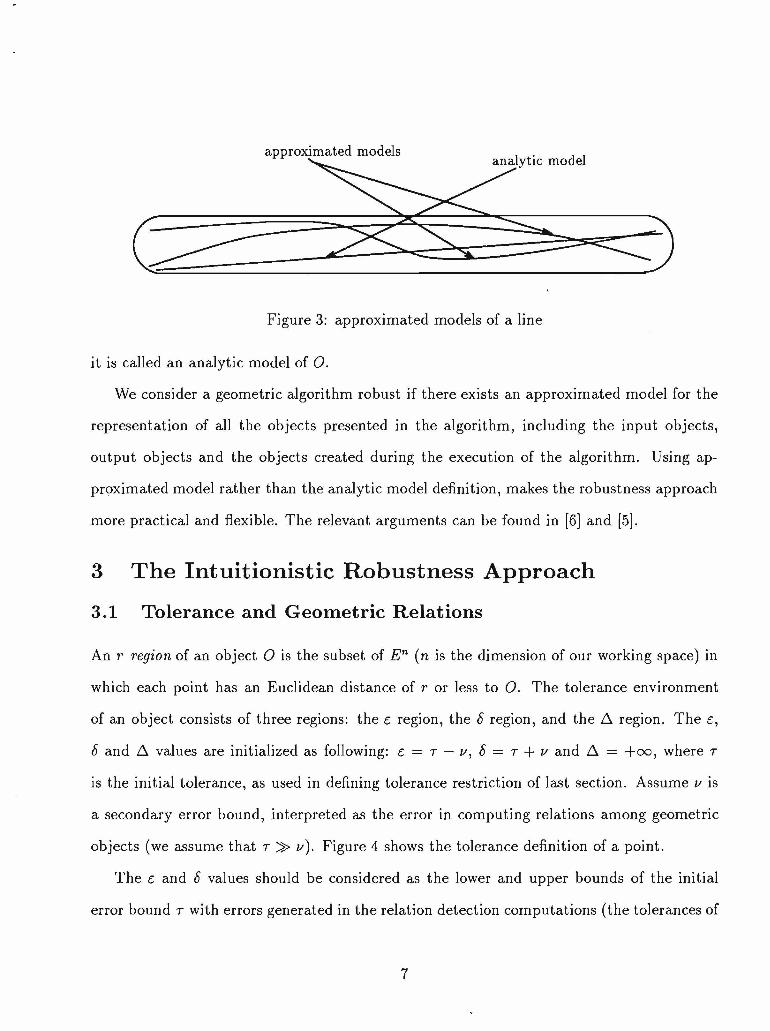
We define that an object M in Euclidean space is an approximated model of an object O

(with representation R ) iff M satisfies the tolerance restriction of O and all the constraints

of R but we don’t require it to have the exact mathematical form of O. So, an approximated

model of object O approximates the shape of object O. For example, in figure 3, the

approximated model of a line can be a curve. IF M also has the same mathematical form,

derived from equality and apartness relations.

6

We consider a geometric algorithm robust if there exists an approximated model for the

representation of all the objects presented in the algorithm, including the input objects,

output objects and the objects created during the execution of the algorithm. Using ap­

proximated model rather than the analytic model definition, makes the robustness approach

more practical and flexible. The relevant arguments can be found in [6] and [5].

3 T h e I n t u i t i o n i s t i c R o b u s t n e s s A p p r o a c h

3 .1 T o l e r a n c e a n d G e o m e t r i c R e l a t i o n s

An r region of an object 0 is the subset of E n (n is the dimension of our working space) in

which each point has an Euclidean distance of r or less to 0 . The tolerance environment

of an object consists of three regions: the £ region, the 8 region, and the A region. The e,

8 and A values are initialized as following: e = t — v , 8 = t + v and A = +oo, where r

is the initial tolerance, as used in defining tolerance restriction of last section. Assume u is

a secondary error bound, interpreted as the error in computing relations among geometric

objects (we assume that r v). Figure 4 shows the tolerance definition of a point.

The e and 8 values should be considered as the lower and upper bounds of the initial

error bound r with errors generated in the relation detection computations (the tolerances of

Figure 3: approximated models of a line

it is called an analytic model of 0 .

7

Figure 4: Initial tolerance definition of a point

related geometric objects and the secondary error v). A regions are used to separate “apart”

objects. The following rules are used to detect relations between two geometric objects and

update their tolerances.

• If the 8 regions of two objects 0\ and 0 2 do not intersect, they are apart (0\ /

0 2). The A value of each object will be updated to be half of the smallest distance

between these two objects if this A value is larger than this distance, otherwise A stays

unchanged.

• If there exists a common approximated model for two objects 0\ and 0 2, the two

objects are coincident (0\ — 0 2). They will then be merged into one single object 0 .

The £ and A regions of 0 are the maximal possible regions of 0 inside the intersections

of the previous £ and A regions of 0\ and 0 2, respectively. The 8 region of 0 is the

minimal region of the 0 enclosing the union of the previous 8 regions of 0 \ and 0 2

(see Figure 5).

• For two objects 0\ and 0 2, if there exists an approximated model of 0 1, Mi, and an

approximated model of 0 2, M2, so that Mi is incident on M2 as objects in Euclidean

space, then 0\ is incident on (0\ C 0 2)- 0 1 will then be updated to the represen­

tation of its approximated model. The new £ and A regions of 0\ are the maximal

8

Figure 5: Tolerance update of two coincident points

9

Figure 6: Point-Curve incidence relations

regions of 0\ inside the intersections of the e and A regions of the old 0\ and 0 2,

respectively. The object O2, its tolerance environment and the 8 region of 0\ stay

unchanged. Figure 6 shows a possible tolerance configuration in which several points

are incident on a curve (only e and 8 regions are shown).

• If two objects have neither coincidence nor incidence relations, and their e regions

intersect, then the two objects are intersecting. The tolerances of the intersection

objects of are defined in such a way that the intersections objects are incident on both

the original objects.

• When the tolerance of an object 0 is updated, all the tolerances of those objects

that have been detected to be incident on 0 also need to be updated so that the

incidence relations still hold, i. e. the e and A regions of these objects must be shrunk

(if necessary) so that they are inside the e and A regions of O respectively.

• If the e region is empty or the 8 region is not totally included in the A region for some

object, then an ambiguity is detected. An ambiguity handling mechanism needs to be

invoked to solve the ambiguity, as described in section 3.3.

10

5

3 .2 R o b u s t n e s s a n d P r o p e r t i e s

The tolerance updating rules, applied after the computation of any relation, ensure that

there is always an approximated model for the representation of all the objects presented

such that all the previously detected relations as well as the newly detected relation hold, as

long as no ambiguity has been found. In other words, the algorithm is robust if it terminates

normally (without ambiguity).

In [5] we proved that the following and other properties are guaranteed by the robustness

method introduced in section 3.1.

• The coincidence relation is an equivalence relation.

• the incidence relation has transitivity, i. e. if A C B and B C C , then A d C .

• If A = B and A ± C , then B ± C .

• If A C B and B ^ C , then A ^ C.

• If A C B and A = C , then C C B.

• If A C B and B = C , then A C C.

In [5] additional rules are provided to preserve the properties such as two lines only

intersect at one point, which is not automatically guaranteed by the approximated model

method.

3 .3 A m b i g u i t y H a n d l in g

As indicated in section 3.1, if any e region becomes empty (e < 0) or any 6 region grows out

of its A region (6 > A ), an ambiguity is detected. In this case we can no longer guarantee the

the relations are consistent with each other, i.e. the existence of a model, is not guaranteed.

The algorithm cannot continue before the ambiguity being solved.

An ambiguity means that the algorithm cannot make a consistent set of decisions with the

initial tolerance (the t value). To solve the ambiguity, the t value has to be redefined. The

problem is whether we need to rerun the algorithm with a new tolerance or we can change

the t value dynamically and then continue the algorithm afterwards. It is shown in [5] that

increasing or decreasing t value by an amount d is equivalent to increasing or decreasing all

the e values and 8 values simultaneously by the same amount d, and that if this simultaneous

change of £ and 6 values does not create new ambiguities, all the previously detected relations

stay unchanged. In other words, the initial tolerance value r can be dynamically changed by

changing all the £ and 6 values, and the algorithm can then be continued. However a total

rerun of the algorithm is still necessary when new ambiguities are created by above dynamic

tolerance adjustment. Practical implementation shows that a total rerun of the algorithm is

rarely needed (see section 4.3).

4 R o b u s t B o o l e a n O p e r a t i o n s

We have implemented a robust Boolean operation algorithm in an experimental solid modeler

based on above robustness approach. Solids in this modeler are represented with a hybrid

representation and are bounded by planes and natural quadric surfaces.

4 .1 A H y b r i d R e p r e s e n t a t i o n

The 3D space can be subdivided by a continuous function f ( x , y , z ) into three areas, the

surface F ° and two half spaces F + and F ~, where

F + = { p : f (p) > 0.0}

F ° = {P : f (p) = 0.0}

F ~ = { p : f (p) < 0.0}

12

9

In the half space representation, a solid is represented as the union of a number of generalized

convex bodies (GCBs), which is defined as the intersection of half spaces[2]. i. e. a solid can

be represented as the following normal form:

un̂s '* j

where the union and intersection operations are regularized set operations[25]. The half

space representation is volume based because it uses volume information (half spaces) as the

basic components of the representation, and it is easy to extract volume information (e. g.

test whether a point is inside a solid) from it.

On the other hand, in a boundary representation (B_Rep), a solid is represented by its

boundaries. Boundary hierarchies (faces, rings, edges and vertices) are often used to facilitate

the access of boundary information[25].

The modeler presented here uses a hybrid representation method that combines the half

space representation and the boundary representation to take advantages of both represen­

tation methods, namely easy accesses to both boundary and volume information. As shown

in in Figure 7, an intermediate representation, in which the boundary curves are associated

with each half space, stored as a single unsorted edge-list. These curves will be used to

represent the edges and rings in the B-rep data structure, later.

Because any Boolean operation can be written as a normal form of half spaces, the

Boolean operation algorithm is basically a process of converting a normal form (half space

representation) to an intermediate representation, i. e. evaluating edges from a normal form.

Details of this edge evaluation process can be found in [2]. B_Reps are built from the

intermediate representation only when it is needed by certain applications such as hidden

line removal display.

13

Figure 7: The hybrid representation structure

4 .2 G e o m e t r i c R e l a t i o n s a n d I n t e r s e c t i o n s

Our algorithm is designed to be independent of the implementation of the low level geometric

relation detection operations. Details of computing geometric relations and the consistency

tests using tolerances are hidden from the main algorithm and implemented in an inde­

pendent tolerance processing module, which primarily performs the operations of tolerance

definition, computation, updating and ambiguity handling.

4.2.1 G eom etric Intersections

For Boolean operations on solids, we must determine the relation between two surfaces

using our robustness method, and find intersections of the two surfaces if they are detected

intersecting. Algebraic solutions are available for relation detections of planes and natural

quadric surfaces.

An approach of finding all the conic section intersections of two natural quadrics is used

based on Goldman and Miller’s work[8]. The paper gives a complete set of all the special

cases occurring when two natural quadric surfaces intersect in one or more conic sections,

using a case by case geometric analysis approach. An example is shown in figure 8 in which

three quadric surfaces intersect in a single ellipse.

Levin’s parametric approach[18], which uses piecewise linear segments to approximate

the intersection curves, is used to find other general intersections of two quadric surfaces.

However, a piecewise linear approximation requires much larger tolerances to be used in the

algorithm which in turn creates more ambiguous relations between objects. Therefore, using

algebraic methods as we do for the special cases, is more efficient and more robust.

For geometric intersections, if the intersection computation involves approximation errors,

these errors should be considered in the tolerance updating process. For example in Figure 9,

two curves intersect at a point with their linear approximations. In building the tolerance

I I I I I

Figure 9: intersecting two curves with tolerances

of the intersection point, the approximation error must be subtracted from £ and A to

guarantee that the point is incident on the two curves.

4.2.2 In s id e /O u ts id e /O n Tests

The inside/outside/on test for a solid, which is a key operation for a volume-based repre­

sentation, can be done entirely with the half space representation and is redefined for our

representation, based on tolerance regions e, 8 and A.

Definition 1 (inside/outside a regularized solid)

A point P is inside a solid iff P is inside one o f the GCBs of the solid or P is on the

boundary of more than one G CB and the two implicit surfaces in the two different G CBs on

which P is incident are coincident with opposite surface normals at P .

A point P is outside a solid iff P is outside all the GCBs of the solid.

A point P is on the boundary of a solid iff P is neither inside nor outside the solid.

A point P is inside a G CB iff P is inside all the half spaces of the GCB.

A point P is outside a G CB iff P is outside one of the half spaces of the GCB.

A point P is on the boundary of a G CB iff P is neither inside nor outside the GCB.

A point P is inside a half space F + iff P and F are apart and P is on the positive side

of F .

A point P is outside a half space F + iff P and F are apart and P is on the negative

side of F .

□

Ambiguous relations that might occur during the computation are solved automatically

as described in 3.3.

4 .3 T e s t s

Two identical cubes of dimensions 100 x 100 x 100, one rotated about all three axis with an

angle a, are tested for Boolean union operation. The initial tolerance r = IE — 3, secondary

error v = IE — 4. Following cases are tested:

• When a > l.ShE — 6, the two cubes intersect.

• When a = l.S E — 6, ambiguities are created, after r is increased to AE — 3, they are

detected coincident.

• When a = 1.5E — 6, ambiguities are created, after r is increased to 3E — 3, they are

detected coincident.

• When a — IE — 6, ambiguities are created, after r is increased to 2E — 3, they axe

detected coincident.

18

• When a < 0.9E — 6, The two cubes are detected coincident

Ambiguities in this example only occur in a very small range, namely for angles 1.8.E—6 >

A > \E — § (about a factor of two). In a previous approachfuiis range was about 10.E4,

roughly 5000 times bigger. The main difference is that we are not using an analytical model,

but an approximated model now, which is more forgiving, but still maintains the desired

properties.

In another test example, we use two identical cylinders with radius 50 and height 400,

one rotated about X axis with an angle /?, and then do a Boolean union of them, r and v are

defined the same as the last example. Five pictures from this test example are shown at the

end of this paper. When angle /? < 0.000001, ambiguities are created. Increasing tolerance

r will solve all the ambiguities, and result in two coincident cylinders.

When we position the two cylinders parallel to each other, they intersect in two straight

line. The second intersection which occurred previously no longer exists.

5 C o n c l u s i o n s

A new tolerance-based robustness method is introduced and applied to Boolean set opera­

tions on 3D objects bounded by planes and natural quadric surfaces. The algebraic methods

for detecting conic section intersections for natural quadric surfaces, together with our toler­

ance based, intuitionistic robustness approach generate very reliable and efficient geometric

algorithms.

The robustness method used in this paper is very general and can be applied to other

geometric algorithms without any changes. In our implementation we completely abstracted

away the low level geometric operations (computing intersections an geometric relations)

from the high level application specific algorithms. This advantage makes the approach bet­

ter suitable as an underlying abstract data type for CAD systems (where different algorithms

1

19

9

access the same model data) than previously published special reasoning solutions.

6 A c k n o w l e d g m e n t s

This work has been supported, in part, by NSF grants DDM-89 10229 and ASC-89 20219,

and a grant from the Hewlett-Packard Laboratories. All opinions, findings, conclusions, or

recommendations expressed in this document are those of the authors and do not necessarily

reflect the view of the sponsoring agencies.

R e f e r e n c e s

[1] BRUDERLIN, B . Detecting ambiguities: An optimistic approach to robustness problems

in computational geometry. Tech. Rep. UUCS 90-003 (submitted), Computer Science

Department, University of Utah, April 1990.

[2] BRUDERLIN, B . Robust regularized set operations on polyhedra. In Proc. of Hawaii

International Conference on System Science (January 1991).

[3] C H O U , S. C . Mechanical Geometry Theorem Proving. D. Reidel Publ., Doordrecht,

Holland, 1988.

[4] EDELSBRUNNER, H., AND M u c k e , E. Simulation of simlicity: A technique to cope

with degenerate cases in geometric algorithms. In Proc. o f 4th A C M Symposium on

Comp. Geometry (June 1988), pp. 118-133.

[5] FANG, S. Robustness in geometric modeling - an intuitionistic and toleranced-based

approach. Ph.D dissertation, University of Utah, Computer Science Department, 1992.

[6] FANG, S., AND B r u d e r l i n , B . Robustness in geometric modeling - tolerance based

methods. In Computational Geometry - Methods, Algorithms and Applications, Inter­

■ 20

9

national Workshop on Computational Geometry C G ’91 (March 1991), Springer Lecture

Notes in Computer Science 553, Bern, Switzerland.

[7] FANG, S., AND BRUDERLIN, B . Robust geometric modeling with implicit surfaces. In

Proc. of International Conference on Manufacturing Automation, Hong Kong (August

1992).

[8] G O L D M A N , R. N., AND M i l l e r , J. R. Combining algebraic rigor with geometric

robustness for the detection and calculation of conic sections in the intersection of

two natural quadric surfaces. In Proc. of the A C M /S IG G R A P H Symposium on Solid

Modeling Foundations and C A D /C A M Applications (June 1991), Austin Texas.

[9] GR EEN E, D., AND Y a o , F. Finite resolution computational geometry. In Proc. 27th

IE E E Symp. Fundations o f Computer Science (1986), pp. 143-152.

[10] GUIBAS, L., S a l ESIN, D., AND STOLFI, J. Epsilon geometry: Building robust algo­

rithms from imprecise computations. In Proc. of 5th A C M Symposium on Computational

Geometry (1989).

[11] HO FF M ANN , C. M. Geometric and Solid Modeling: An Introduction. Morgan Kauf-

mann Publishers, 1989, ch. 4.

[12] HOFFMANN, C. M. The problems of accuracy and robustness in geometric computation.

IE E E Computer 22, 3 (March 1989), 31-41.

[13] H o f f m a n n , C. M ., H o p c r o f t , J. E., AND K a r a s i c k , M. S. Towards implementat-

ing robust geometric computations. In Proc. of 4th A C M Symposium on Computational

Geometry (June 1988), pp. 106-117.

[14] H o f f m a n n , C. M., H o p c r o f t , J. E., a n d K a r a s i c k , M. S. Robust set operations

on polyhedral solids. IE E E Computer Graphics and Application 9 (November 1989).

21

[15] K A P U R , D. Using grobner bases to reason about geometry. J. Symbolic Comp. 2 (1986),

399-408.

[16] KA RA SI C K, M. On the representation and manipulations of rigid solids. Ph.D thesis,

McGill University, 1989.

[17] KU TZ LE R, B. Algebraic approaches to automated geometry proving. Ph.D Diss., Re­

port 88-74.0, Research Institute for Symbolic Comp., Kepler University, Linz, Austria,

1988.

[18] LEVIN, J. A parametric algorithm for drawing pictures of solid objects composed of

quadric surfaces. Communications o f A C M 19, 10 (October 1976), 555-563.

[19] MlLENKOVIC, V . Verifiable implementations of geometric algorithm using finite preci­

sion arithmetic. Artificial Intelligence 37 (1988), 377-401.

[20] M lL E N K O V IC , V . Verifiable implementations of geometric algorithm using finite preci­

sion arithmetic. Ph.D thesis, Carnegie Mellon University, 1988.

[21] M lL E N K O V IC , V. Calculating approximate curve arrangement using rounded arith­

metic. In A C M Annual Symposium on Computational Geometry (1989), pp. 197-207.

[22] M lL E N K O V IC , V ., AND Nackm an, L. R. Finding compact coordinate representations

for polygons and polyhedra. In A C M Annual Symposium on Computational Geometry

(1990), pp. 244-252.

[23] M U D U R , S. P., AND KO PAR KA R, P. A. Interval methods for processing geometric

objects. IE E E Computer Graphics and Application 4, 2 (February 1984), 7 - 17.

[24] OTTMANN, T ., TlIIEMT, G ., AND ULLRICH, C. Numerical stability of geometric

algorithms. In A C M Annual Symposium on Computational Geometry (June 1987),

pp. 119-125.

22

[25] ReqUICHA, A . A. G. Representation for rigid solids: Theory, methods and systems.

C om p u tin g S u rveys 12 , 4 (December 1980).

[26] SALESIN, D. Epsilon geometry: Building robust algorithms from imprecise computa­

tions. Ph.D thesis, Stanford University, 1991.

[27] SALESIN, D., STOLFI, J., AND GuIBAS, L. Epsilon geometry: Building robust al­

gorithms from imprecise calculations. In A C M A n n u a l S ym p osiu m on C om p u ta tion a l

G e o m e tr y (1989), pp. 208-217.

[28] SEGAL, M. Using tolerances to guarantee valid polyhedral modeling results. C o m p u te r

G ra p h ics 2 4 , 4 (1990), 105-114.

[29] STEWART, A. J. Robust point location in approximate polygons. In 1991 C anadian

C o n fe re n c e on C om pxita tion al G e o m etr y (August 1991), pp. 179-182.

[30] STEWART, A. J. The theory and practice of robust geometric computation, or, how to

build robust solid modelers. Ph.D Thesis 91-1229, Department of Computer Science,

Cornell University, 1991.

[31] SUGIIIARA, K ., AND IRI, M. Geometric algorithms in finite precision arithmetic. Res.

Mem. 88-14, Math. Eng. and Information Physicas, University of Tokyo, 1988.

[32] SUGIHARA, K., AND IRI, M. A solid modeling system free from topological inconsis­

tency. J ou rn a l o f In fo rm a tio n P ro cess in g 12 , 4 (1989), 380-393.

[33] TROELSTRA, A. S. C o n stru c tiv ism in M a th em a tic s : A n In trod u ction . Elsevier Science

Pub. Co., 1988.

[34] Yap, C. K. A geometric consistency theorem for a symbolic perturbation theorem. In

P ro c . o f 4 th A C M S ym p osiu m on C om p . G e o m etr y (June 1988), pp. 134-142.

23

Rotation Angle: 0.489957 (in radians)

9

Translation: (80,0,0)