PHYSICAL REVIEW E 92, 052715 (2015)

Role of connectivity and fluctuations in the nucleation of calcium waves in cardiac cells

Gonzalo Hernandez-Hernandez,1 Enric Alvarez-Lacalle,2 and Yohannes Shiferaw1

1Department of Physics & Astronomy, California State University, Northridge, 18111 Nordhoff Street, Northridge, CA 91330, USA2Barcelona Tech, Barcelona, Spain

(Received 15 August 2015; published 20 November 2015)

Spontaneous calcium release (SCR) occurs when ion channel fluctuations lead to the nucleation of calciumwaves in cardiac cells. This phenomenon is important since it has been implicated as a cause of various cardiacarrhythmias. However, to date, it is not understood what determines the timing and location of spontaneouscalcium waves within cells. Here, we analyze a simplified model of SCR in which calcium release is modeled asa stochastic processes on a two-dimensional network of randomly distributed sites. Using this model we identifythe essential parameters describing the system and compute the phase diagram. In particular, we identify a criticalline which separates pinned and propagating fronts, and show that above this line wave nucleation is governed byfluctuations and the spatial connectivity of calcium release units. Using a mean-field analysis we show that thesites of wave nucleation are predicted by localized eigenvectors of a matrix representing the network connectivityof release sites. This result provides insight on the interplay between connectivity and fluctuations in the genesisof SCR in cardiac myocytes.

DOI: 10.1103/PhysRevE.92.052715 PACS number(s): 87.16.A−, 87.19.Hh, 87.10.Mn

I. INTRODUCTION

Calcium (Ca) is a ubiquitous secondary messenger that isresponsible for a vast array of subcellular signaling processessuch as muscle contraction, cell proliferation, and genetranscription [1]. Ca plays a particularly important role in thecardiac cell as it mediates the coupling between membranevoltage and tissue contraction [2]. A central role in Caregulation is played by the ryanodine receptor (RyR) whichcontrols the flow of Ca from intracellular Ca stores to the cellinterior. An important feature of RyR channels is that they arehighly sensitive to Ca and transition from a closed to openstate in a Ca-dependent manner. This Ca sensitivity, which ismediated by multiple binding sites on the channel, is furtheramplified by the close arrangement of RyR channels intoclusters of 10–100 RyR channels [2]. This architecture ensuresthat small increases of local Ca concentration can trigger adomino like opening of an array of RyR channels, leading to alarge local release of Ca [3]. In a cardiac cell there are severalthousand of these clusters organized along equally spacedplanes (Z planes), so that signaling is determined by the numberand timing of these release events. This signaling architectureis found in a wide variety of cell types and is utilized to controlthe spatiotemporal distribution of Ca in the cell [1].

The nonlinear response of RyR receptors in clusters endowsthe Ca cycling system with the properties of an excitablemedium. This is because Ca released at a given cluster candiffuse and activate its nearest neighbors. Thus, under certainconditions a fire-diffuse-fire wave can propagate in the cell[4–6]. These Ca propagation events are referred to as sponta-neous Ca release (SCR) since the release that occurs in thisfashion is typically initiated by a random opening of a single orgroup of RyR clusters [4]. These spontaneous Ca waves playan important role in the genesis of cardiac arrhythmias sincethey can lead to membrane depolarization, which, if it occursin a population of cells, can induce a focal excitation that prop-agates in heart tissue [7–9]. These excitations are dangerousbecause their timing is random and they can therefore disruptthe regular beating of the heart and initiate cardiac arrhythmias[8,10,11]. Despite a great deal of work the basic features of

spontaneous Ca waves (SCR) are still not fully understood.Experimental and theoretical studies reveal a wide rangeof complex spatiotemporal dynamics of Ca depending uponphysiological conditions and cell type [12–16]. In particularBar et al. [12] studied stochastic spreading in an array ofdiscrete sites and identified a nonpropagating to propagatingtransition. Interestingly, the propagation dynamics could bedescribed as a directed percolation process, and also as adepinning transition depending upon the system parameters.More recently, Nivala et al. [15] performed numerical andexperimental studies to explore the emergence of SCR as afunction of sarcoplasmic reticulum (SR) load. These authorsfound that at low SR loads Ca sparks typically occur inthe cell in a stochastic manner but rarely transition to Cawaves. However, as the SR load is increased Ca waves arenucleated in the cell interior with greater frequency; althoughthe distance of propagation is small, i.e., the waves tend to failafter propagating a distance of several micrometers. Furtherincreases in SR load led to longer propagation distances untilwaves propagate the extent of the cell leading to a substantialrelease of Ca. In earlier work Marchant and Parker [17] usedfluorescence imaging to analyze the nucleation of Ca wavesin Xenopus oocytes. In these cells Ca release is governedby clusters of inositol (1,4,5)-triphosphate (IP3) receptorswhich mediate the flow of Ca in similar fashion as do RyRsin cardiac cells. They found that waves tend to nucleate atspecific regions of the cell characterized by a higher densityof release sites and sensitivity to stimulation. Furthermore,they noticed that when the period between Ca waves waslong then wave nucleation occurred at specific sites withgreater reliability. While these studies shed light on variousaspects of subcellular Ca dynamics, several questions remainunanswered. For example, it is not known how the spatialdistribution of calcium release units (CRUs) combines withfluctuations and excitability to determine the location of wavenucleation sites in the cell.

In this paper we explore a simplified theoretical modelthat can be used to understand essential features of Ca wavenucleation and propagation. We analyze in detail the role of

1539-3755/2015/92(5)/052715(13) 052715-1 ©2015 American Physical Society

HERNANDEZ-HERNANDEZ, ALVAREZ-LACALLE, AND SHIFERAW PHYSICAL REVIEW E 92, 052715 (2015)

the random arrangement of CRUs inside the cell, the strengthof diffusive coupling, and the kinetics of spark activation andextinguishing. Our goal is to determine how these propertiesdetermine the location and timing of spontaneous Ca wavesin cardiac cells. Using this approach, we show that thedynamics of SCR is crucially dependent on two importantparameters. The first is the ratio of the length scale overwhich Ca diffuses from a Ca spark to the average distancebetween release sites in the cell, which gives a measure ofthe degree of coupling between CRUs in a cell. The secondparameter is the amount of Ca released during a Ca spark,which determines the excitability of the system. We find thatfor large excitability, fluctuations play the leading role in thespatiotemporal dynamics of the system. In this regime Cawaves are nucleated randomly in the system, and the spatialarrangement of release sites does not determine the sites ofwave nucleation. However, as the excitability is reduced itis the spatial arrangement of Ca release sites which dictatesthe location of wave nucleation. More precisely, we showthat the sites of wave nucleation are determined by eigenvec-tors of the network connectivity matrix, which represents thestrength of diffusive coupling between CRUs. Using a mean-field theory we argue that the initiation of SCR can be viewedas a barrier escape process, which favors wave nucleation atthe sites of eigenvector localization. These results help explainseveral key experimental observations of Ca wave nucleationin biological cells [17]. In particular, they give a quantitativeapproach to identify sites that are prone to initiate Ca waves,and explain why wave nucleation occurs at these sites, withhigher likelihood, as the system excitability is reduced.

II. THE MODEL

A. Biophysical background

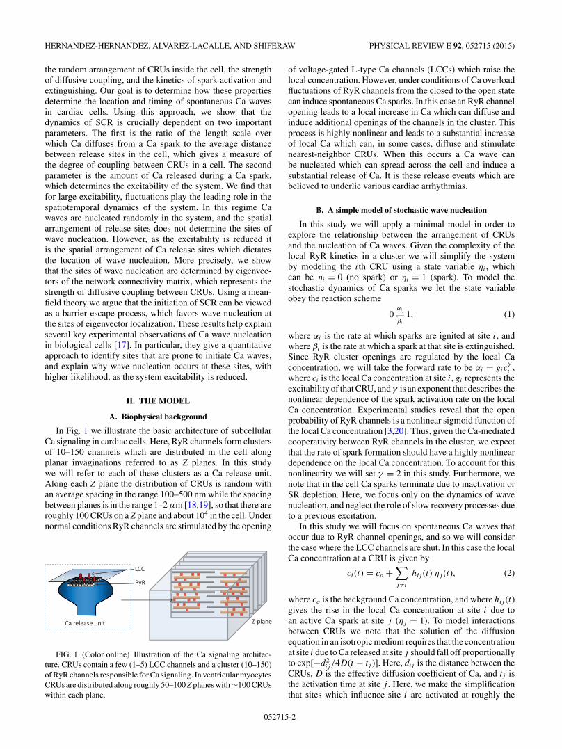
In Fig. 1 we illustrate the basic architecture of subcellularCa signaling in cardiac cells. Here, RyR channels form clustersof 10–150 channels which are distributed in the cell alongplanar invaginations referred to as Z planes. In this studywe will refer to each of these clusters as a Ca release unit.Along each Z plane the distribution of CRUs is random withan average spacing in the range 100–500 nm while the spacingbetween planes is in the range 1–2 μm [18,19], so that there areroughly 100 CRUs on a Z plane and about 104 in the cell. Undernormal conditions RyR channels are stimulated by the opening

FIG. 1. (Color online) Illustration of the Ca signaling architec-ture. CRUs contain a few (1–5) LCC channels and a cluster (10–150)of RyR channels responsible for Ca signaling. In ventricular myocytesCRUs are distributed along roughly 50–100 Z planes with ∼100 CRUswithin each plane.

of voltage-gated L-type Ca channels (LCCs) which raise thelocal concentration. However, under conditions of Ca overloadfluctuations of RyR channels from the closed to the open statecan induce spontaneous Ca sparks. In this case an RyR channelopening leads to a local increase in Ca which can diffuse andinduce additional openings of the channels in the cluster. Thisprocess is highly nonlinear and leads to a substantial increaseof local Ca which can, in some cases, diffuse and stimulatenearest-neighbor CRUs. When this occurs a Ca wave canbe nucleated which can spread across the cell and induce asubstantial release of Ca. It is these release events which arebelieved to underlie various cardiac arrhythmias.

B. A simple model of stochastic wave nucleation

In this study we will apply a minimal model in order toexplore the relationship between the arrangement of CRUsand the nucleation of Ca waves. Given the complexity of thelocal RyR kinetics in a cluster we will simplify the systemby modeling the ith CRU using a state variable ηi , whichcan be ηi = 0 (no spark) or ηi = 1 (spark). To model thestochastic dynamics of Ca sparks we let the state variableobey the reaction scheme

0αi�βi

1, (1)

where αi is the rate at which sparks are ignited at site i, andwhere βi is the rate at which a spark at that site is extinguished.Since RyR cluster openings are regulated by the local Caconcentration, we will take the forward rate to be αi = gic

γ

i ,where ci is the local Ca concentration at site i, gi represents theexcitability of that CRU, and γ is an exponent that describes thenonlinear dependence of the spark activation rate on the localCa concentration. Experimental studies reveal that the openprobability of RyR channels is a nonlinear sigmoid function ofthe local Ca concentration [3,20]. Thus, given the Ca-mediatedcooperativity between RyR channels in the cluster, we expectthat the rate of spark formation should have a highly nonlineardependence on the local Ca concentration. To account for thisnonlinearity we will set γ = 2 in this study. Furthermore, wenote that in the cell Ca sparks terminate due to inactivation orSR depletion. Here, we focus only on the dynamics of wavenucleation, and neglect the role of slow recovery processes dueto a previous excitation.

In this study we will focus on spontaneous Ca waves thatoccur due to RyR channel openings, and so we will considerthe case where the LCC channels are shut. In this case the localCa concentration at a CRU is given by

ci(t) = co +∑j �=i

hij (t) ηj (t), (2)

where co is the background Ca concentration, and where hij (t)gives the rise in the local Ca concentration at site i due toan active Ca spark at site j (ηj = 1). To model interactionsbetween CRUs we note that the solution of the diffusionequation in an isotropic medium requires that the concentrationat site i due to Ca released at site j should fall off proportionallyto exp[−d2

ij /4D(t − tj )]. Here, dij is the distance between theCRUs, D is the effective diffusion coefficient of Ca, and tj isthe activation time at site j . Here, we make the simplificationthat sites which influence site i are activated at roughly the

052715-2

ROLE OF CONNECTIVITY AND FLUCTUATIONS IN THE . . . PHYSICAL REVIEW E 92, 052715 (2015)

80

8884

92

1000 500

1500 2000

1000 1500 2000

500

(ms)

(ms)

(ms)

(a)

(d)

(b)

(c)

FIG. 2. (Color online) Spatiotemporal evolution of active sites in a system with N = 1000 CRUs and L = 1. The ith site is placed atlocation (xi,yi), where xi and yi are picked from a uniform distribution on the interval [0,1]. (a) Ca sparks are nucleated at localized regionsand spread rapidly as an advancing front of active sites. In this case system parameters are chosen to be s = 4 and r = 0.3. Snapshots of activesites at the times shown are indicated. (b) For reduced excitability and coupling (s = 3, r = 0.1) active sites spread in a diffuse manner andsettle in a disordered fluctuating pattern. (c) When the coupling is further reduced only a few sites are activated and randomly distributed inclumps in the system (s = 1, r = 0.8). (d) The total number of active sites n(t) as a function of time for the three cases shown in (a)–(c). Thelocation of sites is the same for all simulation runs.

same time, so that the weighting of distant sites is mostlydetermined by the exponential dependence on d2

ij . To modelthis effect we will consider coupling between CRUs of the form

hij = rj exp[−|�xi − �xj |2/l2], (3)

where rj represents the Ca released at site j , �xi and �xj arethe locations of the ith and j th CRUs in the cell, and l is adiffusive length scale. Alternatively, we note that Ca buffersin the intracellular space will also determine the concentrationof Ca away from the source. This problem has been addressedin detail [21], and it is found that the concentration away froma source of Ca should decay as ∼(1/dij ) exp(−dij / l), wherel is a length scale that is dependent on the buffer kinetics anddiffusivity. In both cases the site-to-site coupling is effectivelyshort ranged and is characterized by a length scale l whichwill be systematically varied in our model.

C. System parameters

To model the spatial distribution of active sparks in acell we will study the time evolution of our system in twodimensions (2D). Thus, we consider the dynamics of N

CRUs that are placed at random locations on a square ofsize L × L, so that the ith site is placed at location (xi,yi),where xi and yi are chosen from a uniform distribution inthe interval [0,L]. This arrangement introduces a length scalewhich is the average minimum distance between CRUs. Thisdistance can be estimated to be d ∼ L/2

√N , so that a natural

dimensionless parameter that characterizes the system is theratio s = l/d = 2

√N l/L, which gives a measure of the length

scale of diffusive interactions compared to the average CRUspacing. Hereafter, we will refer to the parameter s as thespatial coupling strength. In this study we will consider thecase where each CRU is equivalent so that αi = α, βi = β,

gi = g, and ri = r . Also, we take the diffusive length scaleto be a constant with lij = l, so that the heterogeneity inthe system originates only from the spatial arrangement ofCRUs on the plane. The parameter r will be referred to asthe excitability of the system since it gives a measure of theamount of Ca released at a CRU. To fix the system parameterswe will rely on existing experimental observations of Ca sparksand waves. First, we will assume that Ca can diffuse betweennearest neighbors depending on the amount of Ca releasedat each CRU. At high SR loads we expect that Ca releasedat a CRU can diffuse to several nearest neighbors so that wewill consider spatial coupling in the range 0 < s < 6. Also,we will also take co = 0.01 μM and let the spark rate of anisolated CRU be α ∼ 0.001 ms−1, which is roughly one sparkevery second. Since α = gc2

o this will fix g = 0.5 ms−1 μM−2.Finally, we note that since a Ca spark typically lasts for aduration 20–50 ms, we will take β = 0.05 ms−1.

D. Spatiotemporal dynamics

In Figs. 2(a)–2(c) we show the spatiotemporal evolution ofactive sites starting with initial conditions such that all sites are

052715-3

HERNANDEZ-HERNANDEZ, ALVAREZ-LACALLE, AND SHIFERAW PHYSICAL REVIEW E 92, 052715 (2015)

(a) (c)

(b)

No-propagation

Propagation

09

2718

(ms)

FIG. 3. (Color online) (a) The evolution of a planar front of active sites. Initial conditions are chosen such that ηi = 1 for x < 1/2 andηi = 0 for x > 1/2. Filled circles represent active sites at the indicated times. System parameters are s = 4 and r = 0.2. (b) Evolutionof wave front is tracked by averaging ηi in the y direction in bins of size �x = 1/40. (c) Wave propagation threshold in parameterspace.

inactive (ηi = 0). Our numerical simulations reveal that thereare two distinct phases of the system. In one case, illustrated byFig. 2(a), Ca sparks are nucleated at localized regions of thesystem and proceed to spread rapidly as an advancing frontof active sites, with ηi = 1, which invades the surroundinginactive region with ηi = 0. In Fig. 2(a) we show the spatialdistribution of active sites for a short time interval followingnucleation of the advancing front. In this regime the totalnumber of active sites, denoted as n(t), increases rapidly once awave is nucleated [Fig. 2(d), red trace], and the system settles toa final steady state where most of the sites are in the active state.In the case where the excitability and coupling are reduced wesee that waves are not nucleated in the system [Fig. 2(b)].Here, the system slowly evolves towards a state where activesites form a sparse random pattern, where each unit fluctuateswith time according to the local stochastic dynamics. In thiscase, the evolution of the spatial pattern does not occur via acoherent activation front but rather in a gradual fashion wherethe pattern of activity spreads in a diffuse manner. In this casewe find that the number of active sites increases on a muchslower time scale [Fig. 2(d), blue trace]. As the coupling isreduced further [Fig. 2(c)] the spreading of active sites occurseven more slowly, and settles in a sparse random pattern whereonly a few sites are active [Fig. 2(d), green trace]. Here, wefind that the steady state is governed by clumps of active sitesspread randomly throughout the system. These distinct casesare representative of the possible spatiotemporal evolution ofthe system.

E. The propagation and timing of Ca waves

An important feature of the spatiotemporal dynamics is thenucleation of propagating Ca waves. To analyze the dynamicsof waves we study the evolution of a front in 2D that joinsa region of high activity with ηi = 1 with an inactive regionwith ηi = 0. Our goal is to determine the conditions for which

the planar front advances in our system. To investigate thistransition in the most simple setting we chose initial conditionssuch that all points on our L × L square with x � L/2 areset to the value ηi = 1, and all points x > L/2 are ηi = 0[Fig. 3(a)]. To track the evolution of the front we average ηi

in the y direction in bins of size �x = 1/40 along the x axis.In Fig. 3(b) we show the time evolution of this projection,showing that fronts can propagate from the active to theinactive state. Analysis of these fronts reveals that for a givenexcitability r there is a critical coupling sw, which we willrefer to as the front propagation threshold, such that frontswill propagate with s > sw but remain pinned for s < sw.In Fig. 3(c) we plot the function sw(r) which separates thepropagating and nonpropagating regions of phase space.

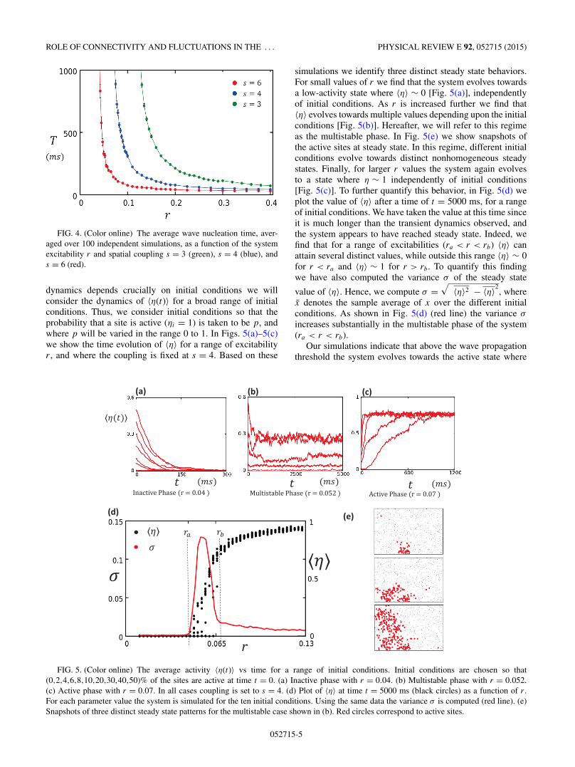
To characterize the timing of wave nucleation we choseinitial conditions so that all sites are inactive (ηi = 0), anddetermine the average waiting time T for a Ca wave to benucleated in the system. Our criterion for wave nucleation isthat the fraction of active sites exceeds 80% of the total numberof CRUs in the system. In Fig. 4 we plot the average wavenucleation time, averaged over 100 independent simulations,as a function of the system excitability r, and for a range ofvalues of the spatial coupling s. This result reveals that as theexcitability r is reduced the wave nucleation time increasessubstantially. Specifically, we find that as r approaches thepropagation threshold the first passage time T appears todiverge. In practice, simulation times become exceedinglylarge and we show results only up to a mean waiting timeof T = 1000 ms.

F. Steady state dynamics

To further characterize the system we have computed thelong-time dynamics of active sites. Thus, we compute thetime dependence of the average number of active sites, whichwe define as 〈η(t)〉 = (1/N )

∑Ni=1 ηi . Since the steady state

052715-4

ROLE OF CONNECTIVITY AND FLUCTUATIONS IN THE . . . PHYSICAL REVIEW E 92, 052715 (2015)

FIG. 4. (Color online) The average wave nucleation time, aver-aged over 100 independent simulations, as a function of the systemexcitability r and spatial coupling s = 3 (green), s = 4 (blue), ands = 6 (red).

dynamics depends crucially on initial conditions we willconsider the dynamics of 〈η(t)〉 for a broad range of initialconditions. Thus, we consider initial conditions so that theprobability that a site is active (ηi = 1) is taken to be p, andwhere p will be varied in the range 0 to 1. In Figs. 5(a)–5(c)we show the time evolution of 〈η〉 for a range of excitabilityr , and where the coupling is fixed at s = 4. Based on these

simulations we identify three distinct steady state behaviors.For small values of r we find that the system evolves towardsa low-activity state where 〈η〉 ∼ 0 [Fig. 5(a)], independentlyof initial conditions. As r is increased further we find that〈η〉 evolves towards multiple values depending upon the initialconditions [Fig. 5(b)]. Hereafter, we will refer to this regimeas the multistable phase. In Fig. 5(e) we show snapshots ofthe active sites at steady state. In this regime, different initialconditions evolve towards distinct nonhomogeneous steadystates. Finally, for larger r values the system again evolvesto a state where η ∼ 1 independently of initial conditions[Fig. 5(c)]. To further quantify this behavior, in Fig. 5(d) weplot the value of 〈η〉 after a time of t = 5000 ms, for a rangeof initial conditions. We have taken the value at this time sinceit is much longer than the transient dynamics observed, andthe system appears to have reached steady state. Indeed, wefind that for a range of excitabilities (ra < r < rb) 〈η〉 canattain several distinct values, while outside this range 〈η〉 ∼ 0for r < ra and 〈η〉 ∼ 1 for r > rb. To quantify this findingwe have also computed the variance σ of the steady state

value of 〈η〉. Hence, we compute σ =√

〈η〉2 − 〈η〉2, where

x denotes the sample average of x over the different initialconditions. As shown in Fig. 5(d) (red line) the variance σ

increases substantially in the multistable phase of the system(ra < r < rb).

Our simulations indicate that above the wave propagationthreshold the system evolves towards the active state where

(b) (c)

tt tActive Phase (r = 0.07 )

(a)

Multistable Phase (r = 0.052 ) Inactive Phase (r = 0.04 )

(d)

r

(

⟩

(e)

FIG. 5. (Color online) The average activity 〈η(t)〉 vs time for a range of initial conditions. Initial conditions are chosen so that(0,2,4,6,8,10,20,30,40,50)% of the sites are active at time t = 0. (a) Inactive phase with r = 0.04. (b) Multistable phase with r = 0.052.(c) Active phase with r = 0.07. In all cases coupling is set to s = 4. (d) Plot of 〈η〉 at time t = 5000 ms (black circles) as a function of r .For each parameter value the system is simulated for the ten initial conditions. Using the same data the variance σ is computed (red line). (e)Snapshots of three distinct steady state patterns for the multistable case shown in (b). Red circles correspond to active sites.

052715-5

HERNANDEZ-HERNANDEZ, ALVAREZ-LACALLE, AND SHIFERAW PHYSICAL REVIEW E 92, 052715 (2015)

FIG. 6. (Color online) The wave propagation threshold (red line)and the transition line separating the monostable active and themultistable phases. The onset of the multistable phase is determinedby finding the parameter r where the variance σ just exceeds 0.05.

〈η〉 ∼ 1. Thus, we expect that the transition from the activeto multistable phase, at r = rb, should coincide with the wavepropagation threshold. To check this hypothesis we have com-pared the wave propagation threshold to the onset of themultistable phase. To determine the onset of the multistablephase we note that the variance σ rises as r is decreased tor = rb [Fig. 5(d)]. Thus, an accurate marker for the onset ofmultistability is the value of r such that the variance has risen tothe value σ = 0.05. In this way we can compute a quantitativeestimate for the onset of the multistable phase. In Fig. 6 wehave plotted the onset of the multistable phase along with thewave propagation threshold. Indeed, we find that these twolines are very close to each other. This result indicates that,as expected intuitively, the onset of the multistable phasecoincides with the threshold for wave propagation.

III. MEAN-FIELD THEORY

A. Deterministic mean-field theory

The numerical simulations of our stochastic spark modelreveal rich spatiotemporal properties. In order to understandbasic features of the system we develop a simplified mean-field theory which will shed light on various aspects of thedynamics. Let us first define the spark probability Pi(t) to bethe probability that the ith CRU is active [ηi(t) = 1] at timet . The stochastic dynamics is then governed by the masterequation

Pi(t + τ ) = [1 − Pi(t)](αiτ ) + Pi(t)(1 − βiτ ), (4)

where αiτ and βiτ are the transition probabilities that site i

makes a 0 → 1 or 1 → 0 transition in the time interval τ . Tosimplify the dynamics we will make the approximation that thestate variables can be replaced by their averages so that ηj ≈Pj , and the local Ca concentration can be approximated byci ≈ co + ∑

j �=i hij Pj (t). In the continuum limit the masterequation then simplifies to the system of equations

dPi

dt= gi

⎛⎝co +

∑j �=i

hijPj

⎞⎠

2

(1 − Pi) − βiPi, (5)

which describes the time evolution of the spark probabilityPi(t).

B. Steady state dynamics of the mean-field equations

To analyze the dynamics of the mean-field equationswe first consider steady state solutions to the N nonlinearequations given in Eq. (5). To distinguish steady state solutionswe keep track of the average site probability defined hereas 〈P (t)〉 = (1/N)

∑Ni=1 Pi(t), and denote the steady state

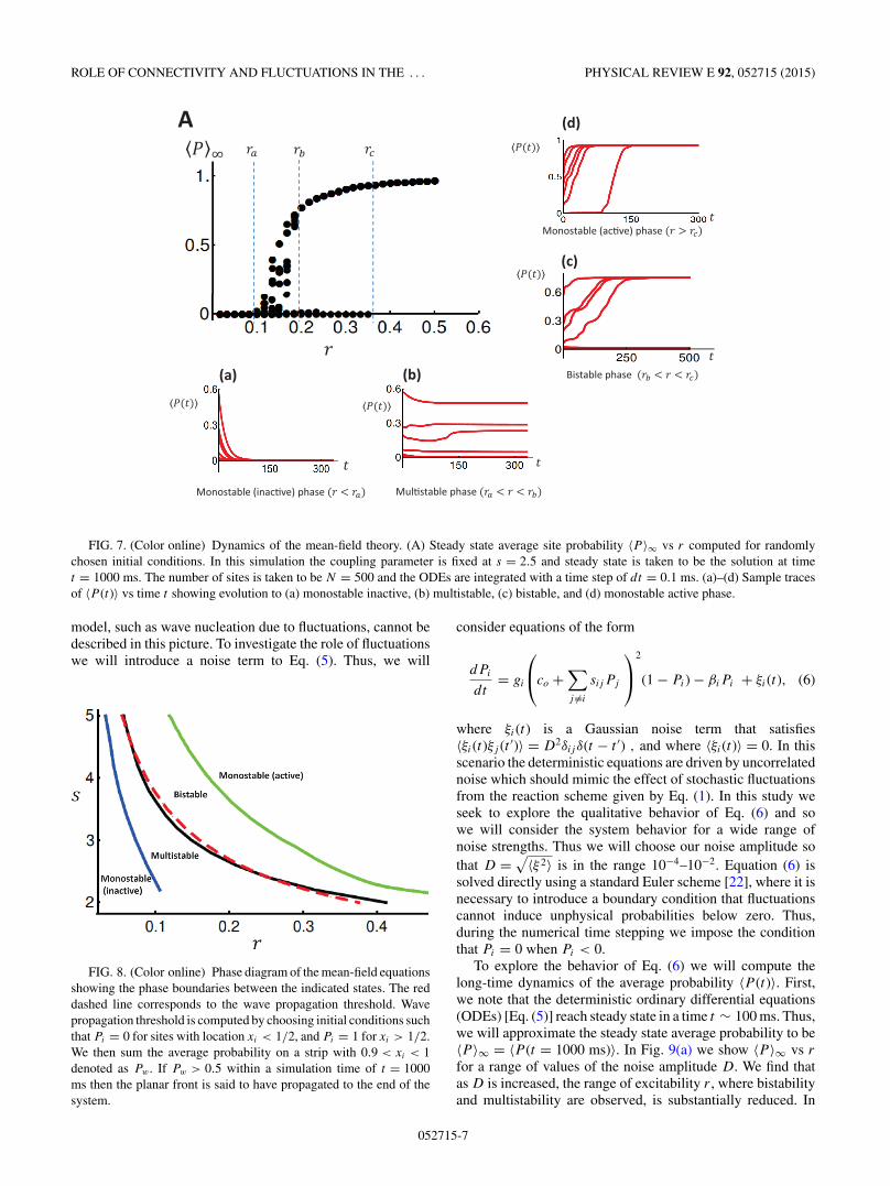
occupation probability as 〈P 〉∞ = 〈P (t → ∞)〉. To capturethe system behavior over a wide range of parameters we willcompute 〈P 〉∞ vs the excitability r , for different values ofthe dimensionless ratio s. As in the full stochastic modelEq. (5) can have multiple steady state solutions, which canbe reached depending upon the initial conditions chosen.Thus, we consider a range of initial conditions of the formPi = p + ξi , where p is an average that will be varied, andwhere ξi is a uniformly distributed random number with anaverage 〈ξ 〉 � p. By considering the time evolution of anensemble of initial conditions, with varying p and 〈ξ 〉, wecan then explore the possible steady state solutions to Eq. (5).Our main results are summarized in Fig. 7(A) where we haveplotted 〈P 〉∞ vs r for a fixed coupling of s = 2.5. We findthat for r < ra then there is effectively only one steady statesolution vector Pi with 〈P 〉∞ ∼ 0 [Fig. 7(a)]. This solutioncorresponds to the inactive state of the system where the steadystate probability of active sites is low. For larger excitability r

we find that there is a region of parameter space between ra andrb where there are multiple steady state solutions which canbe reached depending upon the initial conditions [Fig. 7(b)].However, for larger excitability (rb < r < rc) we find thatthese multiple states collapse into effectively two distinctsolutions. In this regime the system is bistable and can be ineither the active state (〈P 〉∞ ∼ 1) where most sites are active,or the inactive state where the system is quiescent (〈P 〉∞ ∼ 0)[Fig. 7(c)]. For even larger excitability r > rc the lower branchvanishes and the system evolves to a single unique solutionin which 〈P 〉∞ ∼ 1 [Fig. 7(d)]. In order to characterizethe steady state behavior of the mean-field equations wehave constructed the full phase diagram of the mean-fieldtheory. In Fig. 8 we plot the boundaries separating themonostable, bistable, and multistable phases of the mean-fieldequations.

As in the full stochastic model we find that the mean-field equations also possess propagating front solutions. Toinvestigate the wave propagation threshold we simulate thetime evolution of a planar front in 2D which joins the active(Pi = 1) and quiescent (Pi = 0) states. In Fig. 8 we show thewave propagation threshold in parameter space (red dashedline). Above this line a planar front of active sites invadesthe region of inactive sites, while below, the front remainspinned or is extinguished. Indeed, we find that, as in the fullstochastic model, the wave propagation threshold coincideswith the bistability-multistability transition line.

C. The role of fluctuations

A basic limitation of the mean-field theory is that itneglects fluctuations. Thus, key features of the full stochastic

052715-6

ROLE OF CONNECTIVITY AND FLUCTUATIONS IN THE . . . PHYSICAL REVIEW E 92, 052715 (2015)

Monostable (ac�ve) phase )

Bistable phase )

Mul�stable phase )Monostable (inac�ve) phase )

⟩

(a) (b)

(d)

(c)

A

FIG. 7. (Color online) Dynamics of the mean-field theory. (A) Steady state average site probability 〈P 〉∞ vs r computed for randomlychosen initial conditions. In this simulation the coupling parameter is fixed at s = 2.5 and steady state is taken to be the solution at timet = 1000 ms. The number of sites is taken to be N = 500 and the ODEs are integrated with a time step of dt = 0.1 ms. (a)–(d) Sample tracesof 〈P (t)〉 vs time t showing evolution to (a) monostable inactive, (b) multistable, (c) bistable, and (d) monostable active phase.

model, such as wave nucleation due to fluctuations, cannot bedescribed in this picture. To investigate the role of fluctuationswe will introduce a noise term to Eq. (5). Thus, we will

FIG. 8. (Color online) Phase diagram of the mean-field equationsshowing the phase boundaries between the indicated states. The reddashed line corresponds to the wave propagation threshold. Wavepropagation threshold is computed by choosing initial conditions suchthat Pi = 0 for sites with location xi < 1/2, and Pi = 1 for xi > 1/2.We then sum the average probability on a strip with 0.9 < xi < 1denoted as Pw . If Pw > 0.5 within a simulation time of t = 1000ms then the planar front is said to have propagated to the end of thesystem.

consider equations of the form

dPi

dt= gi

⎛⎝co +

∑j �=i

sijPj

⎞⎠

2

(1 − Pi) − βiPi + ξi(t), (6)

where ξi(t) is a Gaussian noise term that satisfies〈ξi(t)ξj (t ′)〉 = D2δij δ(t − t ′) , and where 〈ξi(t)〉 = 0. In thisscenario the deterministic equations are driven by uncorrelatednoise which should mimic the effect of stochastic fluctuationsfrom the reaction scheme given by Eq. (1). In this study weseek to explore the qualitative behavior of Eq. (6) and sowe will consider the system behavior for a wide range ofnoise strengths. Thus we will choose our noise amplitude sothat D =

√〈ξ 2〉 is in the range 10−4–10−2. Equation (6) is

solved directly using a standard Euler scheme [22], where it isnecessary to introduce a boundary condition that fluctuationscannot induce unphysical probabilities below zero. Thus,during the numerical time stepping we impose the conditionthat Pi = 0 when Pi < 0.

To explore the behavior of Eq. (6) we will compute thelong-time dynamics of the average probability 〈P (t)〉. First,we note that the deterministic ordinary differential equations(ODEs) [Eq. (5)] reach steady state in a time t ∼ 100 ms. Thus,we will approximate the steady state average probability to be〈P 〉∞ = 〈P (t = 1000 ms)〉. In Fig. 9(a) we show 〈P 〉∞ vs r

for a range of values of the noise amplitude D. We find thatas D is increased, the range of excitability r , where bistabilityand multistability are observed, is substantially reduced. In

052715-7

HERNANDEZ-HERNANDEZ, ALVAREZ-LACALLE, AND SHIFERAW PHYSICAL REVIEW E 92, 052715 (2015)

(a)

(c)

)

(b)

0

0.5

1.0

FIG. 9. (Color online) Properties of the mean-field equations with noise. (a) Average site probability 〈P 〉∞ vs r computed for ten randomlychosen initial conditions. Here, 〈P 〉∞ is taken to be the average site probability evaluated at time t = 1000 ms. Noise strength is shown on theinset and spatial coupling is set to s = 2.5. ODEs are integrated using a time step of dt = 0.1. (b) Time dependence of 〈P (t)〉. At t = 800 msnoise strength is increased from D = 0 to D = 10−2. Excitability is fixed at r = 0.16. (c) Mean first passage time to wave nucleation computedwith the stochastic mean-field equations. Noise strength is fixed at D = 10−2.

particular, for D = 10−2 the bistable regime is eliminated andthe dispersion of the multistable phase is reduced. The reasonfor this decrease in dispersion is illustrated in Fig. 9(b) wherewe show the effect of noise on the temporal evolution of thesystem. In this simulation we have chosen r = 0.16 so that thedeterministic system is in the multistable phase. For times t <

800 ms we set D = 0 and let the system evolve towards distinctsteady state values depending upon the initial conditions. Fortimes t > 800 ms we turn on noise so that D = 10−2 andobserve that 〈P (t)〉 evolves towards a smaller set of steady statevalues. Here, we find that the steady state behavior attainedin the deterministic limit is unstable to noise perturbationsso that a new set of steady state values is attained once thenoise is turned on. In Fig. 9(c) we plot the mean waitingtime to wave nucleation when the noise amplitude is D =10−2. Indeed, consistent with our stochastic model (Fig. 4),we find that the mean waiting time diverges rapidly as theexcitability is reduced towards the wave propagation threshold.These numerical results indicate that the mean-field equationswith noise capture key features of our stochastic system.

D. Linear stability analysis

Our numerical analysis of the deterministic mean fieldequations [Eq. (5)] reveals a complex phase diagram. A distinctfeature of the system is that for large excitability r > rc thesteady state solution with Pi ≈ 0 becomes unstable, and thesystem always evolves towards the fully active state withPi ≈ 1. To analyze this transition we consider the stabilityof the Pi ≈ 0 solution. In this case we expand Eq. (5) near the

steady state solution p∗i so that Pi = p∗

i + ui , where ui is asmall perturbation. Expanding to linear order in ui gives thelinear system of equations

dui

dt= −[βi + gi (co + qi)

2]ui + 2gi(1 − p∗i )(co + qi)vi,

(7)

where qi = ∑j hijp

∗j , and where vi = ∑

j hijuj . Thus, thestability of the low-activity state is dictated by the system ofequations ui = ∑

j Qijuj where

Qij = −[βi + gi(co + qi)2]δij + 2gi(1 − p∗

i )(co + qi)hij .

(8)

The time evolution of the system is then given by the linearcombination

�u(t) =∑

k

akeλkt

−→φk, (9)

where λk and φk are the eigenvalues and eigenvectors of thematrix Qij . Thus, the quiescent state is unstable when themaximum eigenvalue, which we denote here as λ1, satisfiesthe condition λ1 � 0.

To simplify the analysis further we note that the steadystate occupation probabilities are small so that p∗

i ∼ 0 and1 − p∗

i ∼ 1. We will also assume that each site is identical sothat ri = r and gi = g. Finally, we will make the assumptionthat the terms qi = ∑

j hijp∗j do not vary substantially from

site to site. We have checked this assumption numericallyand find that site-to-site variations in qi have little effect on

052715-8

ROLE OF CONNECTIVITY AND FLUCTUATIONS IN THE . . . PHYSICAL REVIEW E 92, 052715 (2015)

(a) (b)

3

5

6

(c)2

3

S

FIG. 10. (Color online) (a) Ordered components of the leading eigenvector �φ1, with elements normalized so that the maximum is 1. Thesystem size is taken to be N = 1000. (b) Eigenvector components with magnitude larger than 0.5 plotted in the space of points for s = 3 (red),s = 5(blue), and s = 6 (green). (c) Correspondence between high-density regions and eigenvector localization. Blue (red) circles correspondto leading eigenvector components with magnitude larger than 0.5 for parameters s = 2(s = 3). Squares are the regions of highest release sitedensity.

the leading eigenvalues and eigenvectors of the matrix Qij .Hence, we will make the replacement qi → 〈q〉, where 〈q〉 =(1/N )

∑i qi is the site average. This gives an approximation

Qij ≈ −[β + g(co + 〈q〉)2]δij + 2gr(co + 〈q〉) Cij , (10)

where Cij = exp[−|�xi − �xj |2/l2] is the connectivity matrix.The leading eigenvalue is given by λ1 = −[β +g(co + 〈q〉)2] + 2gr(co + 〈q〉)λc, where λc is the leadingeigenvalue of the matrix Cij , and where the spatial evolution ofthe system is governed by the eigenvector which correspondsto λc.

E. Localization of eigenvectors

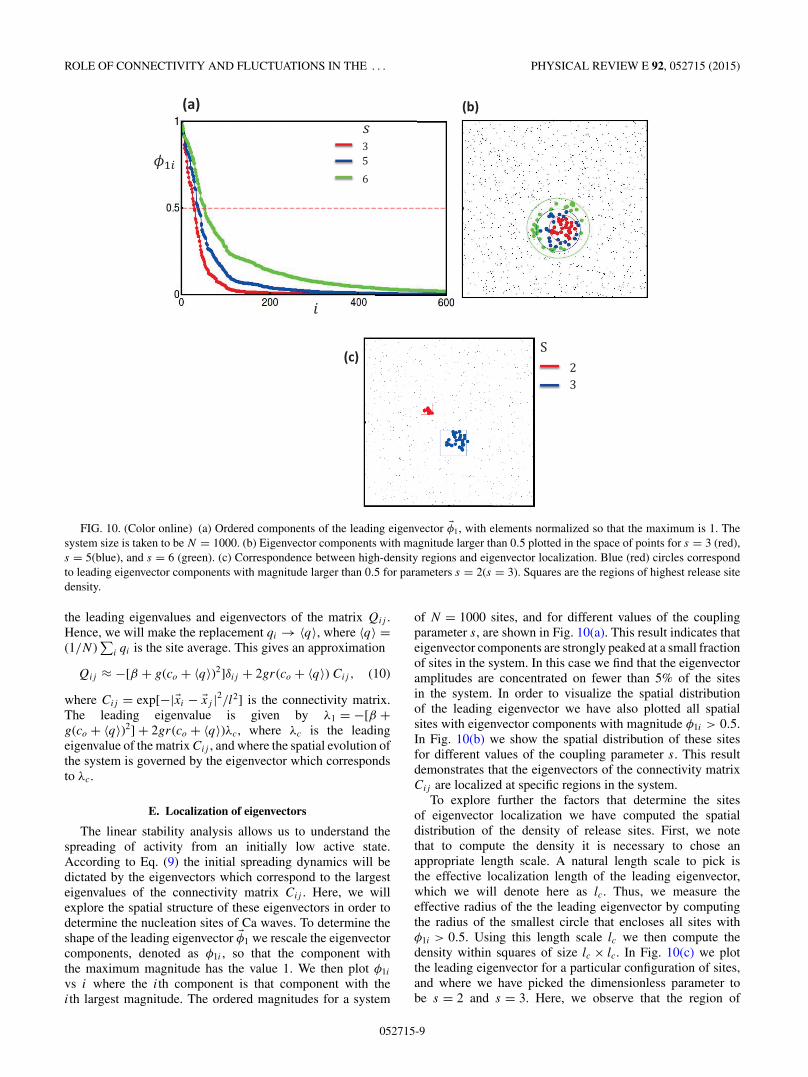
The linear stability analysis allows us to understand thespreading of activity from an initially low active state.According to Eq. (9) the initial spreading dynamics will bedictated by the eigenvectors which correspond to the largesteigenvalues of the connectivity matrix Cij . Here, we willexplore the spatial structure of these eigenvectors in order todetermine the nucleation sites of Ca waves. To determine theshape of the leading eigenvector �φ1 we rescale the eigenvectorcomponents, denoted as φ1i , so that the component withthe maximum magnitude has the value 1. We then plot φ1i

vs i where the ith component is that component with theith largest magnitude. The ordered magnitudes for a system

of N = 1000 sites, and for different values of the couplingparameter s, are shown in Fig. 10(a). This result indicates thateigenvector components are strongly peaked at a small fractionof sites in the system. In this case we find that the eigenvectoramplitudes are concentrated on fewer than 5% of the sitesin the system. In order to visualize the spatial distributionof the leading eigenvector we have also plotted all spatialsites with eigenvector components with magnitude φ1i > 0.5.In Fig. 10(b) we show the spatial distribution of these sitesfor different values of the coupling parameter s. This resultdemonstrates that the eigenvectors of the connectivity matrixCij are localized at specific regions in the system.

To explore further the factors that determine the sitesof eigenvector localization we have computed the spatialdistribution of the density of release sites. First, we notethat to compute the density it is necessary to chose anappropriate length scale. A natural length scale to pick isthe effective localization length of the leading eigenvector,which we will denote here as lc. Thus, we measure theeffective radius of the the leading eigenvector by computingthe radius of the smallest circle that encloses all sites withφ1i > 0.5. Using this length scale lc we then compute thedensity within squares of size lc × lc. In Fig. 10(c) we plotthe leading eigenvector for a particular configuration of sites,and where we have picked the dimensionless parameter tobe s = 2 and s = 3. Here, we observe that the region of

052715-9

HERNANDEZ-HERNANDEZ, ALVAREZ-LACALLE, AND SHIFERAW PHYSICAL REVIEW E 92, 052715 (2015)

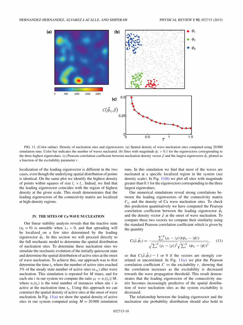
FIG. 11. (Color online) Density of nucleation sites and eigenvectors. (a) Spatial density of wave nucleation sites computed using 20 000simulation runs. Color bar indicates the number of waves nucleated. (b) Sites with magnitude φi > 0.1 for the eigenvectors corresponding tothe three highest eigenvalues. (c) Pearson correlation coefficient between nucleation density vector �ρ and the largest eigenvector �φ1 plotted asa function of the excitability parameter r .

localization of the leading eigenvector is different in the twocases, even though the underlying spatial distribution of pointsis identical. On the same plot we identify the highest densityof points within squares of size lc × lc. Indeed, we find thatthe leading eigenvector coincides with the region of highestdensity at the given scale. This result demonstrates that theleading eigenvectors of the connectivity matrix are localizedat high-density regions.

IV. THE SITES OF Ca WAVE NUCLEATION

Our linear stability analysis reveals that the inactive state(ηi = 0) is unstable when λ1 > 0, and that spreading willbe localized on a few sites determined by the leadingeigenvector �φ1. In this section we will proceed directly tothe full stochastic model to determine the spatial distributionof nucleation sites. To determine these nucleation sites wesimulate the stochastic evolution of the initially quiescent stateand determine the spatial distribution of active sites at the onsetof wave nucleation. To achieve this, our approach was to firstdetermine the time ta where the number of active sites reached3% of the steady state number of active sites (n∞) after wavenucleation. This simulation is repeated for M times, and foreach site i in our system we compute the ratio ρi = ni(ta)/M ,where ni(ta) is the total number of instances when site i isactive at the nucleation time ta . Using this approach we canconstruct the spatial density of active sites at the onset of wavenucleation. In Fig. 11(a) we show the spatial density of activesites in our system computed using M = 20 000 simulation

runs. In this simulation we find that most of the waves arenucleated at a specific localized region in the system (seedensity scale). In Fig. 11(b) we plot all sites with magnitudegreater than 0.1 for the eigenvectors corresponding to the threelargest eigenvalues.

Our numerical simulations reveal strong correlations be-tween the leading eigenvectors of the connectivity matrixCij and the density of Ca wave nucleation sites. To checkthis prediction quantitatively we have computed the Pearsoncorrelation coefficient between the leading eigenvector �φ1

and the density vector �ρ at the onset of wave nucleation. Tocompare these two vectors we compute their similarity usingthe standard Pearson correlation coefficient which is given bythe quantity

C( �ρ, �φ1) =∑N

i (ρi − 〈ρ〉)(φ1i − 〈φ〉)√∑Ni (ρi − 〈ρ〉)2

√∑Ni (φ1i − 〈φ〉)2

, (11)

so that C( �ρ, �φ1) ∼ 1 or 0 if the vectors are strongly cor-related or uncorrelated. In Fig. 11(c) we plot the Pearsoncorrelation coefficient C vs the excitability r , showing thatthe correlation increases as the excitability is decreasedtowards the wave propagation threshold. This result demon-strates that the leading eigenvector of the connectivity ma-trix becomes increasingly predictive of the spatial distribu-tion of wave nucleation sites as the system excitability isdecreased.

The relationship between the leading eigenvector and thenucleation site probability distribution should also hold in

052715-10

ROLE OF CONNECTIVITY AND FLUCTUATIONS IN THE . . . PHYSICAL REVIEW E 92, 052715 (2015)

low activityphase

multistable phase

nucleationdictated by spatial arangementof CRUs

increasing wai�ng �me to wave nuclea�on

wave nucleation dictatedby fluctuations

wavenucleation at

wave propagationtransition

(a) (b)

,

FIG. 12. (Color online) (a) The Pearson correlation between the leading eigenvector �φ1 and the site probability �P (ta) taken at a time tawhere 〈 �P (ta)〉 = 0.1 (red line). The initial conditions are chosen so that 10% of sites are assigned the value Pi(t = 0) = ξi , where ξi is takenfrom a uniform distribution in the range [0,0.5]. Averaging is taken over 5000 simulation runs. For reference we have overlayed the steadystate 〈P 〉∞ of the deterministic mean-field theory (black circles). Dashed line indicates the excitability r = rc separating the monostable andbistable regimes. (b) Illustration of the system phase diagram.

the mean-field theory with noise [Eq. (6)]. To check thisresult we chose parameters above the wave propagationthreshold, and consider the time evolution of a sparse initialpattern with 〈P 〉 ∼ 0. In this parameter regime we measurethe time ta when the average site probability has increasedto 〈P (ta)〉 = 0.1. We then compute the Pearson correlationC( �P (ta), �φ1) where �P (ta) is the probability of release sitesat the onset of wave nucleation. In Fig. 12(a) we plot C

vs r , which shows that the correlation increases as theexcitability r is decreased. On the same graph we overlay thesteady state average 〈P 〉∞ computed using the deterministicmean-field theory. Here, we note that the leading eigenvectoris predictive of the wave initiation sites for r < rc, whichis the regime in which the leading eigenvector is stable(λ1 < 0). These results indicate that the leading eigenvector ispredictive of the sites of nucleation up to the wave propagationthreshold.

V. DISCUSSION

In this paper we have developed a simplified stochasticmodel of Ca wave nucleation in a cardiac cell. In this setting,the spatiotemporal dynamics can be characterized using theexcitability r , which is the amount of Ca released duringa spark, and the spatial coupling s, which is the ratio ofthe distance Ca ions diffuse during a spark to the averagespacing between release sites. In terms of these parameters weshow, in Fig. 12(b), an illustration of the phase diagram ofthe system. Here, we identify a critical line (red dashed line)that separates pinned and propagating excitation fronts. Thistransition line has been observed in previous studies and isdue to the spatial discreteness of the system [12,13]. In effect,the spatial separation between release sites ensures that thereis always a critical excitability below which waves cannotpropagate. A numerical study of the regime of propagationrevealed that the waiting time to a nucleation event diverges asthe excitability is reduced towards the propagation threshold.

Furthermore, we show that as the critical line is approachedwave nucleation tends to occur at regions in which the leadingeigenvector of the connectivity matrix Cij is peaked. In thisregime it is the spatial arrangement of release sites that dictateswhere fluctuations initiate wave nucleation. However, furtheraway from the critical line there is a regime of high excitabilitywhere small fluctuations are sufficient to nucleate waves. Inthis regime fluctuations dominate nucleation kinetics and thearrangement of CRUs does not play an important role. Inparticular, in the limit of large r wave nucleation occurs atthe first 0 → 1 transition, so that wave nucleation occurs atany site with equal probability. Now, below the critical line wealso observe rich dynamical behavior. In particular, we identifya multistable phase where the steady state activity levels formrandom patterns that are dictated by initial conditions. In thisregime waves do not propagate and so there is no mechanismto drive the system to the fully active state. On reducing theexcitability further we also identify a phase where the systemis trapped in a low-activity state. In this regime cooperativitybetween release sites is weak and the system can be describedas a collection of independent sites.

The rich spatiotemporal dynamics of our system can be ex-plained by the interplay between noise and the time evolutionof the deterministic mean-field equations [Eq. (5)]. For largeexcitability (r > rc) the deterministic mean-field equationspossess propagating wave solutions, and the quiescent stateis unstable since λ1 > 0. In this regime wave nucleation isdeterministic and the presence of advancing fronts ensures thatthe same steady state is reached independently of initial condi-tions. In effect, propagating fronts smooth out inhomogeneitiesand the presence of noise does not change the qualitativebehavior of the system dynamics. Now, for rb < r < rc thedeterministic mean-field equations exhibit bistability sincethe quiescent state with Pi ∼ 0 is stable (λ1 < 0). In thisregime fronts advance in the system so that the active branchwith 〈P 〉 ∼ 1 can be reached only if there is a sufficientlylarge region of active sites. Now, in the presence of noise,

052715-11

HERNANDEZ-HERNANDEZ, ALVAREZ-LACALLE, AND SHIFERAW PHYSICAL REVIEW E 92, 052715 (2015)

fluctuations can induce a large enough region of active sitesthat will propagate in the system. Thus, the time evolutionof the quiescent state will be governed by stochastic wavenucleation, which is characterized by a mean-first-passagetime T . In effect, bistability will be observed in the fullystochastic system only if the state of the system is evaluated ata time t < T . For t > T wave nucleation will likely occurand bistability will not be observed, as the system willevolve towards the active branch. Now, in the regime ra <

r < rb the deterministic mean-field equations evolve towardsa multitude of possible steady states. In this phase we findthat active fronts are pinned, so that different steady statescan be reached depending on the initial configuration of activesites. Now, in the presence of noise we find that the systemevolves towards a smaller set of steady states [Fig. 9(b)].This is because noise fluctuations can destabilize a subsetof the steady states that are reached by the deterministicevolution. A pertinent analogy to this behavior is found in thetheory of spin glasses where a disordered system possessesa rugged energy landscape with a large number of energyminima [23]. There, fluctuations due to temperature caninduce transitions between local minima, and the long-timebehavior of the system is governed by the slow dynamicsof stochastic escape between these local minima. However,this dynamics is exceedingly slow since the mean time toescape can be exponentially long. In this case the system issaid to exhibit “glassy” behavior since the system ages overa long time scale, and steady state may not be reached ina tractable simulation time. In effect, the presence of noiseshould drive the system to a unique steady state, but this willlikely take an exceedingly long time. Finally, for r < ra awide range of initial conditions evolve to the same quiescentstate with Pi ∼ 0. In this regime there is effectively only onedistinct steady state and noise does not change the systembehavior.

Our mean-field analysis provides a precise picture of thesites of wave nucleation. In the case when λ1 > 0 wavenucleation is deterministic and the sites of nucleation tend tooccur at the regions where �φ1 is localized. However, in the casewhere the quiescent state is stable (λ1 < 0) we find that theleading eigenvector is still predictive of the sites of nucleation.In fact, our numerical analysis showed that as r is decreasedtowards the propagation threshold, the correlation betweenthe leading eigenvector and the sites of wave nucleationincreases. This result can be explained from the fact that smallfluctuations around the quiescent state evolve according toEq. (10). Thus, fluctuations which occur at regions where �φ1

is localized will decay exponentially at the rate λ1, which isthe slowest decay rate in the system. In effect, the leadingeigenvectors identify preferred regions in the cell where noisefluctuations are most likely to initiate a propagating Ca wave.These results reveal that the eigenvalues and eigenvectors ofthe connectivity matrix play a crucial role in the nucleationdynamics of the system.

Experimental studies have shown that Ca waves cannucleate at specific sites in the cell. In particular, Marchantand Parker [17] imaged Ca waves in the Xenopus oocyte andanalyzed the source of wave nucleation. Indeed, they foundthat Ca waves were nucleated at regions of higher release sitedensity. Also, these sites had a higher than average frequency

of spontaneous firing indicating a higher excitability. Thus,these experiments reveal that both density and excitability playa crucial role in determining those regions in the cell which aremore likely to initiate a Ca wave. Our model analysis predictsthat these sites of wave nucleation correspond to the regionat which the leading eigenvector is localized. Indeed, we findnumerically that the leading eigenvector �φ1 tends to localizein regions of higher density. Furthermore, we have exploredthe role of a heterogeneous distribution of excitabilities (gi),and find that indeed �φ1 will tend to localize in regions ofhigh excitability. However, we have not explored in detail thecompetition between density and excitability in determiningthe sites of localization. Interestingly, Marchant and Parkeralso found that the ability of specific sites to nucleate waveswas more prominent when the interval between Ca waves waslonger. This result is consistent with our main finding that theleading eigenvector becomes more predictive of the nucleationsites as the system excitability is reduced. Hence, theseexperiments confirm our finding that the spatial arrangement ofrelease sites becomes more prominent at reduced excitability.

An important limitation of this study is that we have mod-eled a Ca spark as a simple stochastic on-off process. However,in a cardiac cell, excitation of a Ca spark depends on recoveryfrom inactivation of the RyR channel, or the replenishing ofthe SR load following Ca release. These dynamical processesintroduce refractoriness to each site and will therefore playa crucial role in the location and timing of Ca waves. Forexample, experiments from Nivala et al. [15] have shown thatat high external Ca, Ca waves are nucleated periodically atspecific sites in the cell. However, when the external Ca isdecreased then waves tended to nucleate at random sites in thecell. This result is in contrast to the findings of Marchant andParker who found that as the excitability is reduced then wavestended to originate at specific sites in the cell. This differenceis likely due to the fact that the Ca waves observed in oocyteshave a period larger than 10 s, which is likely much larger thanthe refractory period of release sites. Thus, in this case the ini-tiation of Ca waves is independent of the recovery kinetics, andnucleation sites are dictated by the excitability and arrange-ment of release sites. On the other hand, Nivala et al. observedrepetitive waves with a period ∼1 s. In this case, it is likely thatrecovery kinetics played a crucial role in determining the sitesof wave nucleation. In fact, it is likely that the sites of wave ini-tiation occurred at those regions in which the recovery kineticswas fastest. In the case that recovery kinetics is dictated by therefilling of the SR network, then these sites likely correspondto regions of the cell with a higher density of SR calciumtransport ATPase (SERCA) channels, which are responsiblefor pumping Ca back into the SR. In this study we have notconsidered the role of refractoriness, and therefore our analysisapplies only in the case when the refractory time is much lessthan the average waiting time for a wave nucleation event. Thisis likely the reason why our theoretical results are in excellentagreement with the findings of Marchant and Parker, but notthose of Nivala et al. [15]. A more comprehensive analysis willrequire the inclusion of recovery kinetics in order to extend themodel to the regime when the wave nucleation time is short.

A second limitation of our study is that we have notexplored the role of site-to-site heterogeneities. Experimentalobservations [24] of Ca wave nucleation in astrocytes reveal

052715-12

ROLE OF CONNECTIVITY AND FLUCTUATIONS IN THE . . . PHYSICAL REVIEW E 92, 052715 (2015)

that Ca waves originate at repetitive sites which are stronglycorrelated with regions of the cell with high protein expression,and also with the presence of mitochondria. These resultssuggest that heterogeneities within cells are substantial andplay a crucial role in determining nucleation sites. Also,experimental studies have shown that the distribution of RyRclusters in cardiac myocytes is broadly distributed [25]. Thisresult indicates that clusters with a much larger than averagenumber of channels could potentially drive the initiation ofSCR. To include heterogeneities it will be necessary to includesite disorder in our stochastic simulation and mean-fieldtheory. In this case we expect wave nucleation to still occurat the localization sites of the leading eigenvector of Qij

[Eq. (8)]. These localization sites will be determined by boththe distribution of site disorder and the spatial arrangement ofrelease sites. Hence, while our simplified approach neglectssome key factors, it allows us to study the interplay betweenfluctuations and geometry in the nucleation of Ca waves.Further refinement of these ideas will be necessary to makemore direct contact with experiments.

VI. CONCLUSION

In this study we have introduced a simplified model of Caactivity in a cardiac cell. Using this model we identify theregion in parameter space where the spatial arrangement ofCRUs dictates the sites of wave nucleation. In this regimewe show that wave nucleation occurs at localized regionsdetermined by the eigenvectors of the connectivity matrix.These results serve as a starting point to understand theinterplay between fluctuations and geometry in the formationof Ca waves.

ACKNOWLEDGMENTS

This work was supported by the National Heart, Lung, andBlood Institute Grant No. RO1HL101196. E.A.-L. acknowl-edges funding from the Secretarıa de Estado de Investigacion,Desarrollo e Innovacion (Spain), under Grant No. FIS2011-28820-C02-01.

[1] M. D. Bootman and M. J. Berridge, Cell 83, 675 (1995).[2] D. M. Bers, Nature (London) 415, 198 (2002).[3] H. Cheng and W. J. Lederer, Physiol. Rev. 88, 1491 (2008).[4] L. T. Izu, W. G. Wier, and C. W. Balke, Biophys. J. 80, 103

(2001).[5] T. Takamatsu and W. G. Wier, FASEB J. 4, 1519 (1990).[6] W. Chen, G. Aistrup, J. A. Wasserstrom, and Y. Shiferaw,

Am. J. Physiol: Heart Circulatory Physiol. 300, H1794(2011).

[7] E. G. Lakatta, M. C. Capogrossi, A. A. Kort, and M. D. Stern,Fed. Proc. 44, 2977 (1985).

[8] R. P. Katra and K. R. Laurita, Circulation Res. 96, 535(2005).

[9] W. Chen, M. Asfaw, and Y. Shiferaw, Biophys. J. 102, 461(2012).

[10] R. F. Gilmour, Jr. and N. S. Moise, J. Am. Coll. Cardiol. 27,1526 (1996).

[11] K. R. Laurita and R. P. Katra, J. Cardiovasc. Electrophysiol. 16,418 (2005).

[12] M. Bar, M. Falcke, H. Levine, and L. S. Tsimring, Phys. Rev.Lett. 84, 5664 (2000).

[13] M. Falcke, L. Tsimring, and H. Levine, Phys. Rev. E 62, 2636(2000).

[14] M. Nivala, P. Korge, M. Nivala, J. N. Weiss, and Z. Qu,Biophys. J. 101, 2102 (2011).

[15] M. Nivala, C. Y. Ko, M. Nivala, J. N. Weiss, and Z. Qu,J. Physiol. 591, 5305 (2013).

[16] M. Nivala, C. Y. Ko, M. Nivala, J. N. Weiss, and Z. Qu,Biophys. J. 102, 2433 (2012).

[17] J. S. Marchant and I. Parker, EMBO J. 20, 65 (2001).[18] C. Franzini-Armstrong, F. Protasi, and V. Ramesh, Biophys. J.

77, 1528 (1999).[19] C. Franzini-Armstrong, F. Protasi, and P. Tijskens, Ann. N. Y.

Acad. Sci. 1047, 76 (2005).[20] M. Fill and J. A. Copello, Physiol. Rev. 82, 893 (2002).[21] M. Naraghi and E. Neher, J. Neurosci. 17, 6961 (1997).[22] M. Falcke and D. Malchow, Understanding Calcium Dynamics:

Experiments and Theory, Lecture Notes in Physics No. 623(Springer, Berlin, 2003)

[23] J. A. Hertz and K. H. Fischer, Spin Glasses (CambridgeUniversity Press, Cambridge, 1991).

[24] P. B. Simpson, S. Mehotra, G. D. Lange, and J. T. Russell,J. Biol. Chem. 272, 22654 (1997).

[25] D. Baddeley, I. D. Jayasinghe, L. Lam, S. Rossberger, M. B.Cannell, and C. Soeller, Proc. Natl. Acad. Sci. USA 106, 22275(2009).

052715-13