rotor dynamics measurement techniques - agilent technologies

HeavySpot

CW

PhaseSensor

ProximityProbe

HighSpot

Gap

0°/t0 90°/t1 180°/t2270°/t3 360°/T

1

0.5

0

-0.5

-1

GapAmplitude

phasetime

TachReference

φ = 270°

φ = 270°

30°

-30°

0.866

+j 0.5

-j 0.5

90°+1j

ComplexConjugateVector

Real

Vector

B: Y ORDER REC X:0 RevM:499.51 u* P:206.85deg

Time1-1.266minch 1.266minchAVG: 1

1minch

-1minch

Time 2PolarLag

200uinch

/div

Disp FrmatDate: 08-14-97 Time: 03:41:00 PM

Use the 35670A DataDemonstration Disk(pub. no. 5966-0518E)with this product noteand a 35670A DynamicSignal Analyzer

Rotor Dynamics Measurement Techniques

Product Note: Agilent 35670A-1

2

M A R K E R

Marker

A

MarkerFctn

E

D I S P L AY

MeasData

TraceCoord

Scale

ActiveTrace

Analys DispFormat

B C D

F G H

M E A S U R E M E N T

Freq Window

Input Source Trigger

InstMode

J K L

N O P

R S T

Start PauseCont

Avg

C H 3 C H 4Over

Half

mic pwr

Float ± 4V pk Max

Over

Half

C H 1 C H 2

Source

7 8 9

4 5 6

1 2 3

0 • +/-

I

M

Q

MkrValue

BackSpace

P O W E R

Preset Help BASIC SystemUtility

Plot/Print

U V W

S Y S T E M

Local/HP-IB

DiskUtility

X Y

Save/Recall

Z

F1

F2

F3

F4

F5

F6

F7

F8

F9

Rtn

3 5 6 7 0 ADYNAMIC SIGNAL ANALYZER

3

Contents

Section 1 — Introduction 5

Section 2 — Background 6

Section 3 — Phase Scaling Convention and Conversion 9

Converting to Phase Lag using the Agilent 35670A 11

Phase Lag Scaling 13

Phase Lag Example 14

Section 4 — Slow Roll Removal From Order Records 16

Example: Slow Roll Removal from Order Records 18

Recalling the Data, State, and Math 18

Modifying the Measurement State 19

Display Trace Setup 19

Section 5 — Slow Roll Removal From Orbits 20Example: Slow Roll Removal From Orbits 21

Verify Data Setup 21

Recalling Data 22

Recall Measurement State SLORL2.STA 22

Manual Setup 23

Section 6 — Orbit Rotation to Horizontal and Vertical 24

Example: Orbit Rotation 25

Section 7 — Slow Roll Compensation of Bodé Plots 27

Example: Slow Roll Compensation of Bodé Plots 27

Recalling the Setup 28

Compensated Bodé Plot 30

Section 8 — Shaft Center Line versus Speed or Time 31

Some Cautions 33

Example of Shaft Center Line versus Speed or Time Measurement 34

Recalling the Example Measurement State 34

Manual Setup 35

Section 9 — Order Magnitude-Phase-RPM Numerical Display 36

Example: Numerical Display of Order Magnitude, Phase, and RPM Setup 36

Recalling the Files 37

Measurement State Setup 37

Waveform Math 37

Display Setup 38

Labeling Table Entries 39

Section 10 — Proximity Probe Interfacing 41

Proximity Probe Interfacing 42

Section 11 — Keyphasor Interfacing 43

Keyphasor Tachometer Interfacing 44

Appendix A — Slow Roll Removal 46

Manual Measurement State Setup 46

Appendix B — Shaft Center Line Position Change Versus Speed or Time 47

Manual Measurement State Setup 47

Entering the Math Function F5 47

The Display Setup 48

4

John Jensen is a graduate of SanFrancisco State University, BS inEngineering Science, 1969. He joinedAgilent Technologies shortly aftergraduating and has over 28 years ofpractical experience in physicalmeasurements. During that timeJohn has pioneered the use of electronic test and measurementequipment in electro-mechanical and control system applications. A prolific author, he has written application notes and technical articles for a variety of publications.

Mr. Jensen’s technical expertiseincludes extensive work and publication on a variety of subjectsincluding:

John believes that the challengeof improving product and processperformance through the use of testand measurement techniques andequipment is the most rewarding portion of his work for AgilentTechnologies. He currently providestechnical consulting and support for the complete range of AgilentTechnologies’ Dynamic SignalAnalyzers, Laser positioning systems, Vector Signal Analyzers and Spectrum, Network andImpedance Analyzer products.

John currently makes his home inSan Jose, CA. His wife and 2 childrenkeep life varied and interesting.When not making machinery meas-urements John pursues his hobbies ofwoodworking, travel and gold mining.

About the author:

● Servo Mechanism Testing● Ultrasonic Wire Bonding, ● Process Improvement & Control,● Disk Spindle Bearing Run-out,● Disk Head Flight Dynamics,● Rotating Machinery Fault

Diagnostic Techniques,● Fatigue Damage Detection,● Vibration & Structural Dynamics.

5

This product note is a hands-on tutorial that walks you through implementing often-used data errorcorrection, reduction, and formattingtechniques used in rotating machin-ery diagnostics. The examples willassist prospective users in evaluatingan Agilent Dynamic Signal Analyzer(DSA) for use in rotating machineryanalysis, and veteran users will acquire new tools and techniques tomore accurately and rapidly deter-mine a machine’s condition. The pur-pose of the note is to show you howto use Computed Order Analysis andWaveform Math in Agilent DSAs toassist you in extracting the maximumamount of information available frommachine vibration measurements. Us-ing one instrument with a single userinterface to capture and reduce thedata minimizes the number of incom-patible test instruments needed tomeasure and document a machine’sbehavior. The diagnostician can more

quickly isolate the probable causefrom all the possible causes of exces-sive machine vibration. The notewalks you through the data reductionprocess using setup states and runupvibration data on the 3½” floppy disk(p/n 5966-0518E).

The topics covered are:

Two additional sections cover prox-imity probes and tachometer/keypha-sor interfacing issues with the 35670ADSA. Each section includes step-by-step examples that will assist you inimplementing these functions on an35670A DSA. The examples at the endof each section start by recalling timecapture data, measurement state, andthe waveform math functions to pro-duce results quickly. Then the exam-ple walks you through changes to thedata reduction setup state variablesand display setups to obtain theresults. The changes will illustratehow easy it is to modify the measure-ment state and the effects on theresults. The complete manual setupsequence is provided when appropri-ate. This approach is intended to provide the background and an un-derstanding of the technique, as wellas to help you find your way aroundin the DSA. It is hoped that with abetter understanding of the function-ality in your 35670A, you will beinspired to go beyond what is presented here.

Section 1 Introduction

• Phase Scaling Convention and Conversion

• Slow Roll Removal From X-Y Order Records

• Slow Roll Removal From Orbits

• Orbit Rotation To Horizontal and Vertical

• Slow Roll Compensation of Bodé Plots

• Shaft Centerline Position Versus RPM and/or Time

• Magnitude, Phase, and RPM Numerical Display

6

In rotating machinery diagnosis, a machine – at best – allows only limited access for vibration measure-ments. From this limited set of vibra-tion data, the diagnostician mustrapidly and accurately extract theinformation needed to assess amachine’s condition. The more infor-mation that can be extracted from thevibration data, the better the judg-ment call on the machine’s conditionwill be. These judgment calls havevery expensive consequences, andtherefore speed and accuracy are crit-ical to success. This note is intendedto show the users of Agilent DSAshow to get the maximum amount ofinformation from the available vibra-tion data set. The diagnosticianextracts and enhances the informa-tion from the data by removingerrors, reducing data using differenttechniques, and displaying the resultsin different formats. Each format ordisplay enhances the information indifferent ways. The diagnosticianlooks for consistency in the fault indi-cators and looks for other possibleanomalies or contradictions in themachine’s vibration response data.

Traditionally, to be able to look at data in multiple ways, the diagnos-tician needed to bring a variety ofwidely different kinds of instrumenta-tion to measure and reduce the data.In the past, digital vector filters wereused to examine filtered and unfil-tered orbits, to make Bodé and polar

plots, and read out magnitude, phaseand RPM of an order of rotation. Aspectrum analyzer was required toprovide spectral maps, waterfall spec-trums, etc. An analog or digital taperecorder was used to capture data forfurther analysis. A portable computerand some custom software to controlthe data acquisition and data reduc-tion were often required. Many timesthe data reduction tasks were donemanually or not at all. This all trans-lated into time-consuming andtedious data reduction tasks requiringmany different instruments, all withincompatible and mostly proprietarydata formats.

Order tracking analysis evolved usinganalog/digital tracking filters referredto as digital vector filters (DVFs). TheDVFs provided tracking filters with

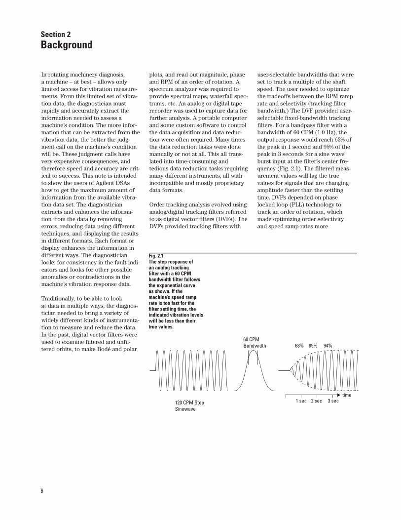
user-selectable bandwidths that wereset to track a multiple of the shaftspeed. The user needed to optimizethe tradeoffs between the RPM ramprate and selectivity (tracking filterbandwidth.) The DVF provided user-selectable fixed-bandwidth trackingfilters. For a bandpass filter with abandwidth of 60 CPM (1.0 Hz), theoutput response would reach 63% ofthe peak in 1 second and 95% of thepeak in 3 seconds for a sine waveburst input at the filter’s center fre-quency (Fig. 2.1). The filtered meas-urement values will lag the truevalues for signals that are changingamplitude faster than the settlingtime. DVFs depended on phaselocked loop (PLL) technology totrack an order of rotation, whichmade optimizing order selectivity and speed ramp rates more

Section 2 Background

Fig. 2.1 The step response of an analog tracking filter with a 60 CPM bandwidth filter follows the exponential curve as shown. If the machine’s speed ramp rate is too fast for the filter settling time, the indicated vibration levels will be less than their true values.

120 CPM StepSinewave

60 CPMBandwidth 63% 89% 94%

time1 sec 2 sec 3 sec

7

complicated (Fig. 2.2). The DVFs interfaced directly to proximityprobes and keyphasor signals as wellas to other transducers. The DVF dis-played shaft RPM, bearing clearances(gap), and phase angle relative to theonce-per-revolution phase reference.Synchronously filtered data could be viewed by connecting an oscillo-scope. Bodé and polar plots were produced by connecting to an analogor digital X-Y plotter. The DVFs werereal workhorses for vibration analysisand are still much admired for theirorbit displays, large numerical readout, and ease of use (Fig. 2.3).

The data acquisition and data reduction speed advantages of thefirst- and second-generation FastFourier Transform-based dynamic sig-nal analyzers made them very attrac-tive prospects for rotating machineryanalysis. Some of these early high-endDSAs were equipped with externalsampling inputs that could interfacewith a machine’s tach signal andcould be triggered from the once-per-revolution keyphasor. An FFT analyz-er could measure hundreds of ordersat one time, which looked very attrac-tive compared to the one order perchannel on a DVF. The realities ofdoing order tracking required an external tracking ratio synthesizer

(TRS) to lock the DSA sampling tothe tach signal from a rotor. The TRSmultiplied the shaft tach so the DSAwas sampling at uniform angles ofrotation. The FFT works best with128, 256, or 512 samples per revolu-tion (2n) and an integer number ofrevolutions in the data record. It was often worth the difficulties to

install a custom tach (toothed wheel)to provide the needed 2n pulses perrevolution just to eliminate the TRS.The TRS could not maintain perfectlock to the shaft rotation as the speedramped up. The tracking of RPM overmultiple speed ranges was also diffi-cult. A digital tracking low pass filteralso was needed to minimize aliasing

Fig. 2.2 The deviation of an “ideal” phase locked loop’s estimate of a shaft’s angular position from the shaft’s actual position for a constant RPM ramp.

Fig. 2.3 The unfiltered orbits in the upper traces produced the filtered orbits in the lower traces. The DVF tracking filters used PLL to tune to the order being filtered.

3.0

2.0

1.0

0.0

RotationAngle

Actual Data

"Ideal" PLLEstimate of Data

Time

TachometerSignal

VERT. Unfiltered = 1.06 Mils, p-p at -5.40 Volts DCHORIZ. Unfiltered = 0.87 Mils, p-p at -5.70 Volts DC

VERT. 1X Vector = 0.94 Mils, p-p at -145°HORIZ. 1X Vector = 0.67 Mils, p-p at -221°

0.40

Mils

/ Di

visi

on0.

40 M

ils /

Divi

sion

CW Rotation

CW Rotation

Speed = 11,288 RPM Sweep Rate = 5 mSec. / Division

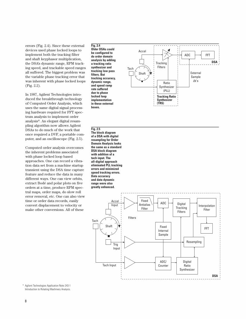
Fig. 2.4 Older DSAs could be configured to do order domain analysis by adding a tracking ratio synthesizer and tracking low pass filters. But tracking accuracy, dynamic range, and speed ramp rate suffered due to phase locked loop implementation in these external boxes.

8

errors (Fig. 2.4). Since these external devices used phase locked loops toimplement both the tracking filterand shaft keyphasor multiplication,the DSA’s dynamic range, RPM track-ing speed, and trackable speed rangesall suffered. The biggest problem wasthe variable phase tracking error thatwas inherent with phase locked loops(Fig. 2.2).

In 1987, Agilent Technologies intro-duced the breakthrough technologyof Computed Order Analysis, whichuses the same digital signal process-ing hardware required for FFT spec-trum analysis to implement orderanalysis*. An elegant digital resam-pling algorithm now allows AgilentDSAs to do much of the work thatonce required a DVF, a portable com-puter, and an oscilloscope (Fig. 2.5).

Computed order analysis overcomesthe inherent problems associatedwith phase locked loop basedapproaches. One can record a vibra-tion data set from a machine startuptransient using the DSA time capturefeature and reduce the data in manydifferent ways. One can view orbits,extract Bodé and polar plots on fiveorders at a time, produce RPM spec-tral maps, order maps, do slow rollerror removal, etc. One can also viewtime or order data records, easilyconvert displacement to velocity ormake other conversions. All of these

Fig. 2.5 The block diagram of a DSA with digital resampling for Order Domain Analysis looks the same as a standard DSA block diagram with addition of a tach input. The all-digital approach eliminated PLL tracking errors and minimized speed tracking errors. Data accuracy and data dynamic range were alsogreatly enhanced.

AccelInput

TachFilters

DSA

ADC DigitalTracking

Filters

InterpolationFilter

FFT

Resampling

DigitalRatio

Synthesizer

ADC/Counter

FixedInternalSample

Tach Input

TrigInput

FixedAntialias

Filter

Shaft

* Agilent Technologies Application Note 243-1 Introduction to Rotating Machinery Analysis.

Accel

Tach

TrackingFilters

ExternalSample

t's∆

ADC FFT

DSA

RatioSynthesizer

(PLL)

Shaft

Tracking RatioSynthesizer(TRS)

9

results can often be produced andplotted in less time than it would take to set up and rewind an analogor digital tape recorder. Accurate cali-brated results can now be viewedquickly, on site, with a minimum ofinstrumentation.

The DSA’s order tracking and orderspectrum filters provide proportionalbandwidth (BW) tracking filters. Thefilter’s bandwidth changes with themachine’s speed. For example, at 600 CPM (10 Hz) and with a deltaorder set to 0.1, the DSA’s tracking fil-ter bandwidth would be 0.1 X 10 Hzor 1 Hz. Because we are using an FFTto produce these filters, the settlingtime equivalent for the 1 Hz BW filteris 1 second. At 6000 CPM (100 Hz),the tracking filter BW is 0.1 X 100 Hzor 10 Hz wide. The settling timeequivalent would be 0.1 second. TheDSA, by default, automatically pro-vides the optimum tracking speedand tracking filter BW. Computedorder analysis equips the DSA withmeasurement capability that can handle higher RPM speed ramp rateswith better phase and amplitudeaccuracy than is possible with phase locked loops.

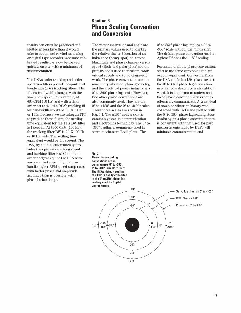
The vector magnitude and angle arethe primary values used to identifythe relative size and location of animbalance (heavy spot) on a rotor.Magnitude and phase changes versusspeed (Bodé and polar plots) are theprimary tools used to measure rotorcritical speeds and to do diagnosticwork. The phase convention used inmachinery vibration, plane geometry,and the electrical power industry is a0° to 360° phase lag scale. However,two other phase conventions are also commonly used. They are the 0° to ±180° and the 0° to -360° scales.These three scales are shown in Fig. 3.1. The ±180° convention is commonly used in communicationand electronics technology. The 0° to -360° scaling is commonly used inservo mechanism Bodé plots. The

0° to 360° phase lag implies a 0° to -360° scale without the minus sign.The default phase convention used inAgilent DSAs is the ±180° scaling.

Fortunately, all the phase conventionsstart at the same zero point and areexactly equivalent. Converting fromthe DSA’s default ±180° phase scale tothe 0° to 360° phase lag conventionused in rotor dynamics is straightfor-ward. It is important to understandthese phase conventions in order toeffectively communicate. A great dealof machine vibration history was collected with DVFs and plotted withthe 0° to 360° phase lag scaling. Stan-dardizing on a phase convention thatis consistent with that used for pastmeasurements made by DVFs willminimize communication and

Section 3 Phase Scaling Convention and Conversion

Fig. 3.1 Three phase scaling conventions are in common use: 0° to -360°, 0° to ±180°, and 0° to 360°. The DSA’s default scaling of ±180° is easily converted to the 0° to 360° phase lag scaling used by Digital Vector Filters.

180° -180°+180-180°

90°

+90°

-90°

-270°

-90°

270°

0° 0°+360°

0°-360°

Servo Mechanism 0° to -360°

DSA Phase ±180°

Phase Lag 0° to 360°

10

interpretation errors. You shouldchoose and use phase and magnitudescales that are historically consistent.In this manner one can avoid possiblydisastrous consequences.

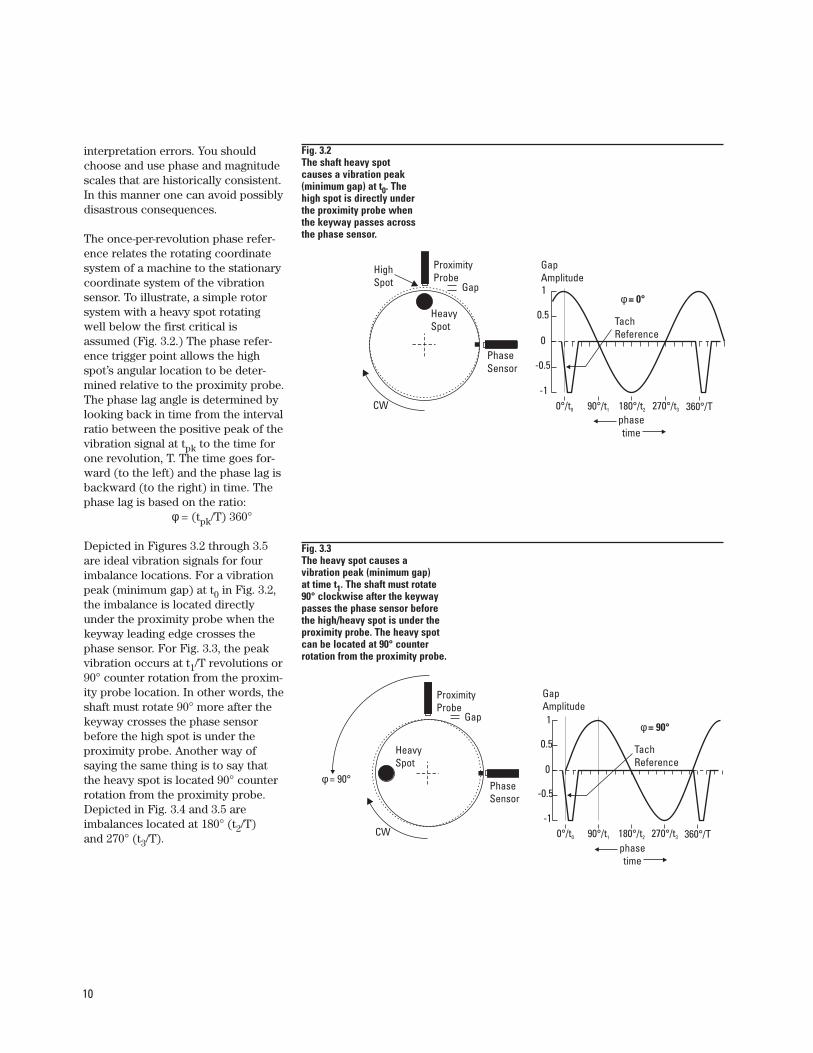
The once-per-revolution phase refer-ence relates the rotating coordinatesystem of a machine to the stationarycoordinate system of the vibrationsensor. To illustrate, a simple rotorsystem with a heavy spot rotatingwell below the first critical isassumed (Fig. 3.2.) The phase refer-ence trigger point allows the highspot’s angular location to be deter-mined relative to the proximity probe.The phase lag angle is determined bylooking back in time from the intervalratio between the positive peak of thevibration signal at tpk to the time forone revolution, T. The time goes for-ward (to the left) and the phase lag isbackward (to the right) in time. Thephase lag is based on the ratio:

φ = (tpk/T) 360°

Depicted in Figures 3.2 through 3.5are ideal vibration signals for fourimbalance locations. For a vibrationpeak (minimum gap) at t0 in Fig. 3.2,the imbalance is located directlyunder the proximity probe when thekeyway leading edge crosses thephase sensor. For Fig. 3.3, the peakvibration occurs at t1/T revolutions or90° counter rotation from the proxim-ity probe location. In other words, theshaft must rotate 90° more after thekeyway crosses the phase sensorbefore the high spot is under theproximity probe. Another way of saying the same thing is to say thatthe heavy spot is located 90° counter rotation from the proximity probe.Depicted in Fig. 3.4 and 3.5 are imbalances located at 180° (t2/T) and 270° (t3/T).

Fig. 3.2 The shaft heavy spot causes a vibration peak (minimum gap) at t0. The high spot is directly under the proximity probe when the keyway passes across the phase sensor.

Fig. 3.3 The heavy spot causes a vibration peak (minimum gap) at time t1. The shaft must rotate 90° clockwise after the keyway passes the phase sensor before the high/heavy spot is under the proximity probe. The heavy spot can be located at 90° counter rotation from the proximity probe.

HeavySpot

CW

PhaseSensor

ProximityProbe

HighSpot Gap

0°/t0 90°/t1 180°/t2 270°/t3 360°/T

1

0.5

0

-0.5

-1

GapAmplitude

phasetime

φ = 0°

TachReference

HeavySpot

CW

PhaseSensor

ProximityProbe

Gap

0°/t0 90°/t1 180°/t2 270°/t3 360°/T

1

0.5

0

-0.5

-1

GapAmplitude

phasetime

φ = 90°

TachReference

φ = 90°

11

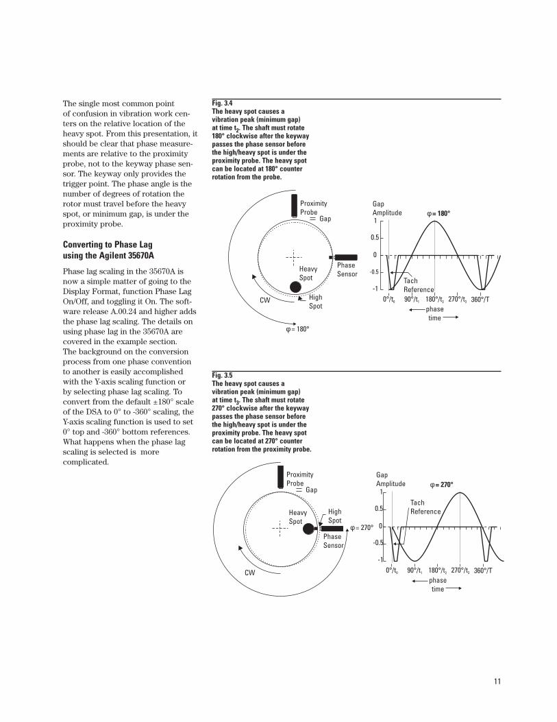
The single most common point of confusion in vibration work cen-ters on the relative location of theheavy spot. From this presentation, itshould be clear that phase measure-ments are relative to the proximityprobe, not to the keyway phase sen-sor. The keyway only provides thetrigger point. The phase angle is the number of degrees of rotation the rotor must travel before the heavyspot, or minimum gap, is under theproximity probe.

Converting to Phase Lag using the Agilent 35670A

Phase lag scaling in the 35670A isnow a simple matter of going to theDisplay Format, function Phase LagOn/Off, and toggling it On. The soft-ware release A.00.24 and higher addsthe phase lag scaling. The details onusing phase lag in the 35670A are covered in the example section. The background on the conversionprocess from one phase conventionto another is easily accomplishedwith the Y-axis scaling function or by selecting phase lag scaling. To convert from the default ±180° scaleof the DSA to 0° to -360° scaling, theY-axis scaling function is used to set0° top and -360° bottom references.What happens when the phase lagscaling is selected is more complicated.

Fig. 3.4 The heavy spot causes a vibration peak (minimum gap) at time t2. The shaft must rotate 180° clockwise after the keyway passes the phase sensor before the high/heavy spot is under the proximity probe. The heavy spot can be located at 180° counter rotation from the probe.

Fig. 3.5 The heavy spot causes a vibration peak (minimum gap) at time t3. The shaft must rotate 270° clockwise after the keyway passes the phase sensor before the high/heavy spot is under the proximity probe. The heavy spot can be located at 270° counter rotation from the proximity probe.

HeavySpot

CW

PhaseSensor

ProximityProbe

HighSpot

Gap

0°/t0 90°/t1 180°/t2 270°/t3 360°/T

1

0.5

0

-0.5

-1

GapAmplitude

phasetime

TachReference

φ = 180°

φ = 180°

HeavySpot

CW

PhaseSensor

ProximityProbe

HighSpot

Gap

0°/t0 90°/t1 180°/t2 270°/t3 360°/T

1

0.5

0

-0.5

-1

GapAmplitude

phasetime

TachReference

φ = 270°

φ = 270°

12

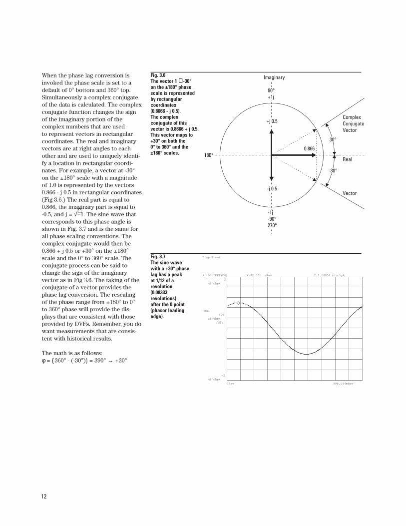
When the phase lag conversion is invoked the phase scale is set to adefault of 0° bottom and 360° top.Simultaneously a complex conjugateof the data is calculated. The complexconjugate function changes the signof the imaginary portion of the complex numbers that are used to represent vectors in rectangularcoordinates. The real and imaginaryvectors are at right angles to eachother and are used to uniquely identi-fy a location in rectangular coordi-nates. For example, a vector at -30°on the ±180° scale with a magnitudeof 1.0 is represented by the vectors0.866 - j 0.5 in rectangular coordinates(Fig 3.6.) The real part is equal to0.866, the imaginary part is equal to-0.5, and j = √−1. The sine wave thatcorresponds to this phase angle isshown in Fig. 3.7 and is the same forall phase scaling conventions. Thecomplex conjugate would then be0.866 + j 0.5 or +30° on the ±180°scale and the 0° to 360° scale. Theconjugate process can be said tochange the sign of the imaginary vector as in Fig 3.6. The taking of theconjugate of a vector provides thephase lag conversion. The rescalingof the phase range from ±180° to 0°to 360° phase will provide the dis-plays that are consistent with thoseprovided by DVFs. Remember, you dowant measurements that are consis-tent with historical results.

The math is as follows:φ = {360° - (-30°)} = 390° → +30°

Fig. 3.6The vector 1 ∠∠-30° on the ±180° phase scale is represented by rectangular coordinates (0.8666 - j 0.5). The complex conjugate of this vector is 0.8666 + j 0.5. This vector maps to +30° on both the 0° to 360° and the ±180° scales.

30°

180°

-30°

0.866

+j 0.5

-j 0.5

90°+1j

-1j-90°270°

ComplexConjugateVector

Real

Vector

Imaginary

Fig. 3.7The sine wave with a +30° phase lag has a peak at 1/12 of a revolution (0.08333 revolutions) after the 0 point (phasor leading edge).

A: D7 IFFT(D8) X:82.031 mRev Y:1.00058 minchpk

0Rev 996.094mRev

2minchpk

-2minchpk

Real400

uinchpk/div

Disp Frmat

13

Phase Lag Scaling

The first part of the example coverssetting up phase lag scaling in the35670A with software release A.00.24and higher. The second part takes youthrough the vector math to providean intuitive handle on the phase lagscaling calculation. As an aid in doingthe example, the DSA’s sequence ofcommands is called out in a compactnotation. The Front Panel push but-tons (hard keys) are shown as:

“Hard Keys”

and the soft buttons, F0 through F9,are shown as:

“SOFT KEYS”

A sequence of commands is connect-ed by “→”. Commands such as MARKER ON OFF → ON indicate that the function is to be toggled to theON state.

Setting up phase lag scaling on the 35670A is simply a matter of activating the feature. (Available infirmware release A.00.24 or higher*.)Phase lag is implemented as a user-selected scaling that is applied to all subsequent phase coordinate dis-plays. To activate the scaling press:

Display format → MORE →PHASE LAG ON / OFF → ON

Turning phase lag on will change thescaling and coordinates for all subse-quent analyzer measurement modes.

The Phase Lag On can be saved in theinstrument state and then recalled.When it is recalled, all phase tracesand coordinates will be set to a phaselag range of 0° to 360° for all othermeasurement modes. If the phase lagscale is the phase convention youwish to use, then save an Autostatewith Phase Lag On. At power up thephase lag scale will be activated.

The key path to save an autostate is:

Save/Recall → SAVE MORE →SAVE AUTOSTATE

Note: Autostate will also store any othersettings such as displays or input ranges.Be sure your 35670A is set-up to your preferences before storing an Autostate.

The phase scale of 0° bottom, 360°top is the default phase lag tracerange, but the user can change thescale to 0° top, 360° bottom. Thecommand sequence is:

Scale → TOP REFERENCE → 0 →BOTTOM → 360

The phase range can be auto-scaledor an arbitrary range can be set using:

Scale → AUTOSCALE ON OFF → ON orScale → TOP REFERENCE and BOTTOMkeys.

All phase plots are labeled PHASELAG when phase lag is turned on.When

Preset → DO PRESET

are pressed, the phase lag scaling willrevert to the default PHASE LAG OFFMODE of scaling (±180°). For the35670A with older software releases(A.00.21 or lower), phase lag scalingcan be implemented using the mathfunction conjugate multiply CONJ( ).The phase scale is set to 0° bottomand to 360° at the top. The state withthe phase lag scale and conjugatemultiply math function would besaved. When recalled, the math andstate/trace can be used to plot phaselag. The 35670A with software rev. A.00.21 or lower will allow aphase scale of 360° top and 0° bot-tom, which is the most commonlyused format for phase lag plots. Forthe FFT linear resolution and com-puted order analysis measurementmodes in the 35670A, a separate conjugate multiply math function for each measurement result that isto be plotted in phase lag coordinateswill be required.

* To order a firmware update for your 35670A in the USA,dial 1-800-452-4844 or in Canada 800-387-3154 and ask fora quote for 35670U Option UE2. This includes the latestfirmware release and an up-to-date manual set.

14

Phase Lag Example

In the example, two simple real-imaginary data records and the conjugate math function are recalledto illustrate the phase lag scale conversion process.

Insert the disk “Agilent 35670A RotorDynamics MeasurementsTechniques”into the analyzer.Press:

Save / Recall → CATALOG ON / OFF → ON

Rotate the marker knob to highlightthe file name “PHZLAG.STA”.Press:

RECALL STATE

Verify that the prompt at the top of the analyzer screen shows“RECALL STATE = PHZLAG.STA”.Press:

ENTER

The state sets up the Order Analysismeasurement mode, display coordi-nates, and format. The recalled state also sets the time and frequencyparameters so the math function op-erates in sync with the recalled data.

Next, with the disk catalog on the display, rotate the marker knob tohighlight the file “PHZLAG.DAT”.Press:

RECALL DATA → RECALL TRACE AND SCALE→ FROM FILE INTO D8.

Verify that “FROM FILE INTO D8 =PHZLAG.DAT” is in the prompt fieldand then press:

ENTER

The recalled real-imaginary data willbe used to demonstrate the phase lagconversion process using the mathfunction that will be recalled later.

With the disk catalog on the display, rotate the marker knob tohighlight file “PHZLG1.DAT” andpress:

FROM FILE INTO D7

Verify that the correct file is in theprompt field and then press

ENTER

Next, with the disk catalog on the display, rotate the marker knob tohighlight the file “PHZLAG.MTH”.Press:

Rtn → Rtn

(the button located just below thesoft key F9) and press:

RECALL MORE → RECALL MATH

Verify that the prompt at the top ofthe screen shows “RECALL MATH =PHZLAG.MTH” and then press:

ENTER

Press Disp Format key to turn on thetrace display. Press:

Active Trace → D Trace Coord → MORE CHOICES →IMAGINARY PART

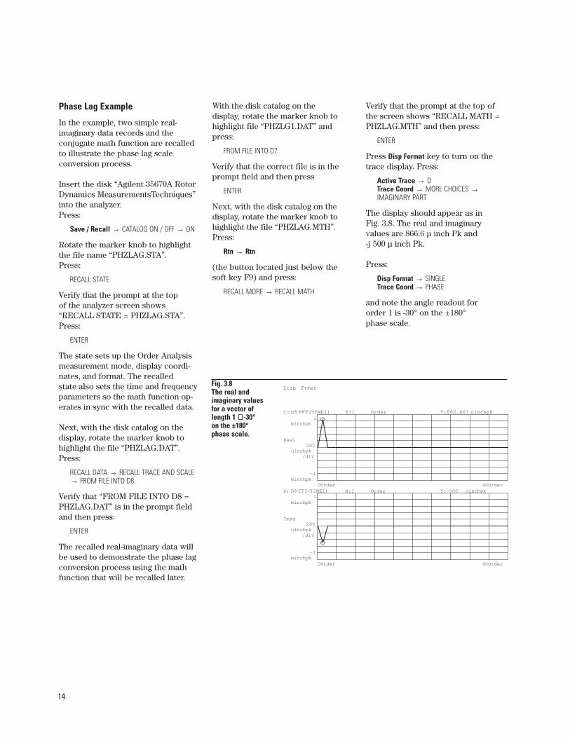
The display should appear as in Fig. 3.8. The real and imaginary values are 866.6 µ inch Pk and -j 500 µ inch Pk.

Press:

Disp Format → SINGLETrace Coord → PHASE

and note the angle readout for order 1 is -30° on the ±180° phase scale.

Fig. 3.8 The real and imaginary values for a vector of length 1 ∠∠-30° on the ±180° phase scale.

Disp Frmat

0Order 40Order

C: D8 FFT(TIME1) X:1 Order Y:866.667 uinchpk1

minchpk

-1minchpk

Real200

uinchpk/div

X:1 Order Y:-500 uinchpkD: D8 FFT(TIME1)1

minchpk

-1minchpk

Imag200

uinchpk/div

0Order 40Order

15

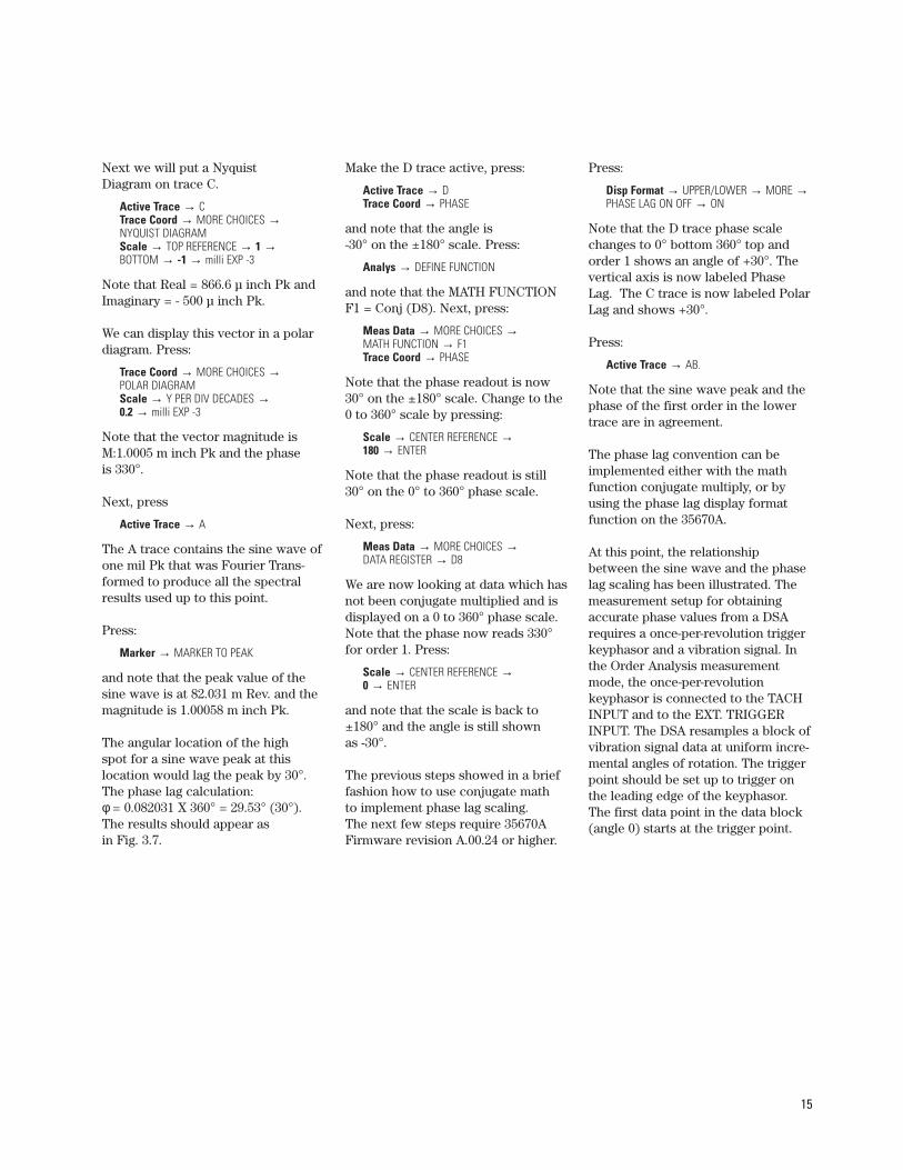
Next we will put a Nyquist Diagram on trace C.

Active Trace → C Trace Coord → MORE CHOICES →NYQUIST DIAGRAM Scale → TOP REFERENCE → 1 →BOTTOM → -1 → milli EXP -3

Note that Real = 866.6 µ inch Pk andImaginary = - 500 µ inch Pk.

We can display this vector in a polardiagram. Press:

Trace Coord → MORE CHOICES →POLAR DIAGRAM Scale → Y PER DIV DECADES →0.2 → milli EXP -3

Note that the vector magnitude isM:1.0005 m inch Pk and the phase is 330°.

Next, press

Active Trace → A

The A trace contains the sine wave ofone mil Pk that was Fourier Trans-formed to produce all the spectralresults used up to this point.

Press:

Marker → MARKER TO PEAK

and note that the peak value of thesine wave is at 82.031 m Rev. and themagnitude is 1.00058 m inch Pk.

The angular location of the high spot for a sine wave peak at this location would lag the peak by 30°.The phase lag calculation: φ = 0.082031 X 360° = 29.53° (30°).The results should appear as in Fig. 3.7.

Make the D trace active, press:

Active Trace → D Trace Coord → PHASE

and note that the angle is -30° on the ±180° scale. Press:

Analys → DEFINE FUNCTION

and note that the MATH FUNCTIONF1 = Conj (D8). Next, press:

Meas Data → MORE CHOICES →MATH FUNCTION → F1 Trace Coord → PHASE

Note that the phase readout is now30° on the ±180° scale. Change to the0 to 360° scale by pressing:

Scale → CENTER REFERENCE →180 → ENTER

Note that the phase readout is still30° on the 0° to 360° phase scale.

Next, press:

Meas Data → MORE CHOICES →DATA REGISTER → D8

We are now looking at data which hasnot been conjugate multiplied and isdisplayed on a 0 to 360° phase scale.Note that the phase now reads 330°for order 1. Press:

Scale → CENTER REFERENCE →0 → ENTER

and note that the scale is back to±180° and the angle is still shown as -30°.

The previous steps showed in a brieffashion how to use conjugate math to implement phase lag scaling. The next few steps require 35670AFirmware revision A.00.24 or higher.

Press:

Disp Format → UPPER/LOWER → MORE →PHASE LAG ON OFF → ON

Note that the D trace phase scalechanges to 0° bottom 360° top andorder 1 shows an angle of +30°. Thevertical axis is now labeled PhaseLag. The C trace is now labeled PolarLag and shows +30°.

Press:

Active Trace → AB.

Note that the sine wave peak and thephase of the first order in the lowertrace are in agreement.

The phase lag convention can be implemented either with the mathfunction conjugate multiply, or by using the phase lag display format function on the 35670A.

At this point, the relationship between the sine wave and the phaselag scaling has been illustrated. Themeasurement setup for obtainingaccurate phase values from a DSArequires a once-per-revolution triggerkeyphasor and a vibration signal. Inthe Order Analysis measurementmode, the once-per-revolutionkeyphasor is connected to the TACHINPUT and to the EXT. TRIGGERINPUT. The DSA resamples a block ofvibration signal data at uniform incre-mental angles of rotation. The triggerpoint should be set up to trigger onthe leading edge of the keyphasor.The first data point in the data block(angle 0) starts at the trigger point.

16

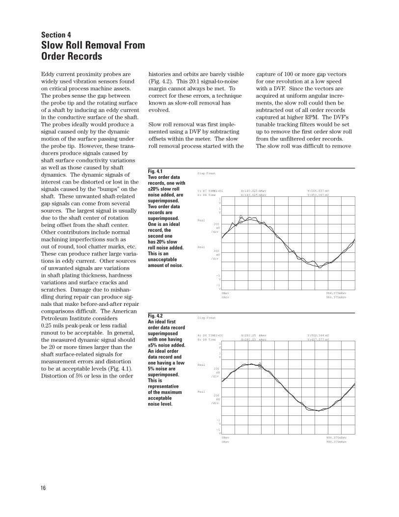
Eddy current proximity probes arewidely used vibration sensors foundon critical process machine assets.The probes sense the gap betweenthe probe tip and the rotating surfaceof a shaft by inducing an eddy currentin the conductive surface of the shaft.The probes ideally would produce asignal caused only by the dynamicmotion of the surface passing underthe probe tip. However, these trans-ducers produce signals caused byshaft surface conductivity variationsas well as those caused by shaft dynamics. The dynamic signals ofinterest can be distorted or lost in thesignals caused by the “bumps” on theshaft. These unwanted shaft-relatedgap signals can come from severalsources. The largest signal is usuallydue to the shaft center of rotationbeing offset from the shaft center.Other contributors include normalmachining imperfections such as out of round, tool chatter marks, etc.These can produce rather large varia-tions in eddy current. Other sourcesof unwanted signals are variations in shaft plating thickness, hardnessvariations and surface cracks andscratches. Damage due to mishan-dling during repair can produce sig-nals that make before-and-after repaircomparisons difficult. The AmericanPetroleum Institute considers 0.25 mils peak-peak or less radialrunout to be acceptable. In general,the measured dynamic signal shouldbe 20 or more times larger than theshaft surface-related signals for measurement errors and distortion to be at acceptable levels (Fig. 4.1).Distortion of 5% or less in the order

histories and orbits are barely visible(Fig. 4.2). This 20:1 signal-to-noisemargin cannot always be met. Tocorrect for these errors, a techniqueknown as slow-roll removal hasevolved.

Slow roll removal was first imple-mented using a DVF by subtractingoffsets within the meter. The slowroll removal process started with the

capture of 100 or more gap vectorsfor one revolution at a low speedwith a DVF. Since the vectors areacquired at uniform angular incre-ments, the slow roll could then besubtracted out of all order recordscaptured at higher RPM. The DVF’stunable tracking filters would be setup to remove the first order slow rollfrom the unfiltered order records.The slow roll was difficult to remove

Section 4Slow Roll Removal From Order Records

Fig. 4.1 Two order data records, one with ±20% slow roll noise added, are superimposed. Two order data records are superimposed. One is an ideal record, the second one has 20% slow roll noise added. This is an unacceptable amount of noise.

Disp Frmat

0Rev 984.375mRev

C: D7 TIME1+D1 X:140.625 mRev Y:566.637 mV

1V

-1V

Real200

mV/div

X:140.625 mRev Y:453.087 mVD: D8 Time

0Rev 984.375mRev

1V

-1V

Real200

mV/div

Fig. 4.2 An ideal first order data record superimposed with one having ±5% noise added. An ideal order data record and one having a low 5% noise are superimposed. This is representative of the maximum acceptable noise level.

0Rev 984.375mRev

A: D6 TIME1+D1 X:281.25 mRev Y:502.364 mV

1V

-1V

Real200

mV/div

X:281.25 mRev Y:457.577 mVB: D8 Time

0Rev 984.375mRev

1V

-1V

Real200

mV/div

Disp Frmat

17

for higher orders. The process wastime consuming and tedious so it was usually done “off line” usingtape-recorded data.

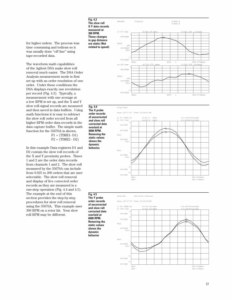
The waveform math capabilities of the Agilent DSA make slow rollremoval much easier. The DSA OrderAnalysis measurement mode is firstset up with an order resolution of oneorder. Under these conditions theDSA displays exactly one revolutionper record (Fig. 4.3). Typically, ameasurement with one average at a low RPM is set up, and the X and Yslow roll signal records are measuredand then saved in data buffers. Usingmath functions it is easy to subtractthe slow roll order record from allhigher RPM order data records in thedata capture buffer. The simple mathfunction for the 35670A is shown.

F1 = (TIME1- D1)F2 = (TIME2 - D2)

In this example Data registers D1 andD2 contain the slow roll records ofthe X and Y proximity probes. Times1 and 2 are the order data recordsfrom channels 1 and 2. The slow rollmeasured by the 35670A can includefrom 0.025 to 200 orders that are userselectable. The slow roll removal and display of live corrected orderrecords as they are measured is aone-step operation (Fig. 4.4 and 4.5).The example at the end of this section provides the step-by-step procedures for slow roll removalusing the 35670A. This example uses300 RPM on a rotor kit. Your slowroll RPM may be different.

0Rev 984.375mRev

A: F1 TIME1-D1 X:437.5 mRev Y:3.00379 minchpk

5minchpk

-5minchpk

Real1

minchpk/div

X:437.5 mRev Y:3.64492 minchpkB: CH1 Time

0Rev 984.375mRev

5minchpk

-5minchpk

Real1

minchpk/div

Disp Frmat

Date: 08-27-97 Time: 03:54:00 PM

Save/Rec Def Disk: Internal

Date: 08-27-97 Time: 03:54:00 PM

0Rev 984.375mRev

C: F2 TIME2-D2 X:703.125 mRev Y:2.86738 minchpk

5minchpk

-5minchpk

Real1

minchpk/div

X:703.125 mRev Y:3.24549 minchpkD: CH2 Time

0Rev 984.375mRev

5minchpk

-5minchpk

Real1

minchpk/div

Fig. 4.4The X probe order records of uncorrected and slow roll corrected data overlaid at 6000 RPM. Removing the static values shows the dynamic behavior.

Fig. 4.5The Y probe order records of uncorrected and slow roll corrected data overlaid at 6000 RPM. Removing the static values shows the dynamic behavior

Fig. 4.3 The slow roll X-Y data records measured at 300 RPM. These changes in gap distance are static (Not related to speed)

Marker Trace:D X Ref: 0Y Ref: 0

0Rev 984.375mRevAVG: 1

C: D7 Time X:406.25 mRev Y:662.325 uinchpk1

minchpk

-1minchpk

Real200

uinchpk/div

X:734.375 mRev Y:392.435 uinchpkD: D8 Time1

minchpk

-1minchpk

Real200

uinchpk/div


18

Example: Slow Roll Removal fromOrder Records

Slow roll removal from order recordshas three conceptual steps. First, theslow roll behavior must be measured.In our example you will extract thisfrom stored rotor kit run-up data.Next the math functions which subtract the slow roll characteristicsfrom live measurements must be defined. In our example you will recall measurement state parameters to set these functions up. Finally, theactual high speed rotor measure-ments are made and the corrected results displayed.

In our supplied example data theslow roll measurements are made at300 RPM. The slow roll measurementtakes advantage of averaging in theanalyzer. For the actual dynamicshaft measurements it is important tonote that the rotor kit used for thisdata has very little dynamic responsebelow 3000 RPM. You’ll be instructedto turn off averaging and to manuallychange the start speed to 3000 RPMand the stop speed to 8000 RPM. Bytriggering the measurement on largerRPM increments (increasing the RPMstep size) you can speed up the meas-urement. RPM step arming will beused to allow you to control the exact trigger conditions of eachmeasurement.

The example, using the supplied capture data, is intended to be aguide for your use. You would usesimilar techniques to make measure-ments from tape recorded data, rotorkits or directly from probes on anoperating machine.

Recalling the Data, State, and Math

The slow roll removal example startsby doing a preset. Press:


The runup data, measurement stateand math functions are recalled next.Insert the disk “Agilent 35670A RotorDynamicsMeasurements Techniques”into the analyzer.Press:


Rotate the marker knob to highlightthe file name “RNUPAC.TIM”.Press:

RECALL DATA → RECALL CAPTURE.

Verify that the prompt at the top of the analyzer screen shows“RECALL CAPTURE =RNUPAC.TIM”.Press:

ENTER

Recalling the time capture file willrequire about one minute.

Rotate the marker knob to highlightthe file “SLOROL.MTH” andthen press:

RtnRECALL MORERECALL MATH

Verify that the prompt at the top of the analyzer screen shows“RECALL MATH = SLOROL.MTH”. Press:

ENTER

Rotate the marker knob to highlightthe file “SLORL1.STA”. Press:

RtnRECALL STATE

Verify that the prompt at the top of the analyzer screen shows“RECALL STATE = SLORL1.STA”.Press:

ENTERDisp FormatStart

The DSA will begin a measurementon the captured rotor data you justrecalled. The tach readout at the topof the screen will increment up to approximately 300 RPM and the X and Y slow roll proximity probewaveforms will appear in the A and Btraces with the markers on their re-spective peaks. The screen shouldmatch the data in Fig. 4.3. This is your measurement of slow roll properties.

The next step is to store the slow rollproperties for use in correctingdynamic measurements. The X-Yslow roll data will be saved in dataregisters D1 and D2. Press:

Active Trace → A → Save Recall →SAVE DATA → SAVE TRACE → INTO D1 Active Trace → B → SAVE TRACE →INTO D2

19

Modifying the Measurement State

The order analysis state will now bemodified to measure from 3000 to8000 RPM. The data display will beset up to show the results of theuncorrected order data overlaid withthe slow roll corrected data.Press:

Avg → AVERAGE ON OFF → OFF

The measurement will be set to startat 3000 RPM and to stop at 8000 RPM.The RPM step size will be increasedto 40 RPM to speed up the measurement.

Freq → MIN RPM → 3000→ RPM →MAX RPM → 8 → KRPMTrigger → ARM SETUP → RPM STEP ARM→ RPM STEP SIZE → 40 → RPM

The display is set up to display themath function results. Press:

Active Trace → A Meas Data → MORE CHOICES →MATH FUNCTION → F1 Active Trace → B → F2Active Trace → A B Trace Coord → MORE CHOICES → REAL PARTStart

to begin the measurement. The tachdisplay will start incrementing up andwhen it reaches 3000 RPM, the slowroll corrected data will appear on thescreen. The slow roll correction willcontinue to update every 40 RPM andstop at approximately 8000 RPM. Thelast measurement at 8000 RPM willappear fixed on the screen.

Display Trace Setup

The following key sequence sets up the display so that the slow rollcorrected and raw data can be com-pared. The trace setup to displayuncorrected X probe data in the Btrace is as follows:Press:

Disp Format → QUAD Active Trace → B Meas Data → TIME CHAN 1

Trace setup to display the slow rollcorrected data for the Y probe intrace C is:

Active Trace → C Meas Data → MORE CHOICES →MATH FUNCTION → F2

Trace setup to display uncorrected Y-probe data in trace D is:

Active Trace → DMeas Data → CHAN 1 2 3 4 → 2 →TIME CHAN 2

All four traces will be set to displaycoordinates Real versus 1 rotationand to autoscale their data.

Active Trace → A B C D Trace Coord → MORE CHOICES → REAL PARTScale → AUTO SCALE ON OFF → ON →OFF

Turning autoscale on, then off, forcesa one time rescaling of the display.

Next set up a front back (overlaid)display of the slow roll corrected and uncorrected X data. The X probe

data will be in traces A and B, the Y probe data will be in traces C and D.

Active Trace → A BMarker → COUPLED ON OFF → ON →MARKER TO PEAKCOUPLED ON OFF → OFF Active Trace → C D →MARKER TO PEAKDisp Format → SINGLE FRNT/BACKActive Trace → A B

This displays the corrected anduncorrected X probe data. Note thatthe slow roll corrected X probe datatrace is about 0.64 mils less than theuncorrected X order data record (Fig. 4.4).

The Y probe uncorrected andcorrected data are examined by

making the C trace active.

Active Trace → C D

The results will be very similar to Fig. 4.5. Note that the slow roll cor-rection is approximately 0.378 mils.The smooth shaft on the rotor kit produced only a small slow roll error.The slow roll correction did not produce significant effects until the dynamic response began to grow at3000 RPM. The first 10 orders wereremoved in one pass. Since this ap-proach is not correcting one order ata time as is possible with a DVF, the results you will see are going to be alittle different. When a slow rollrecord is subtracted from a higherRPM record that is only slightly larg-er, the difference will be dominatedby noise.

A detailed step-by-step key sequence is provided as a reference in Appendix A.

20

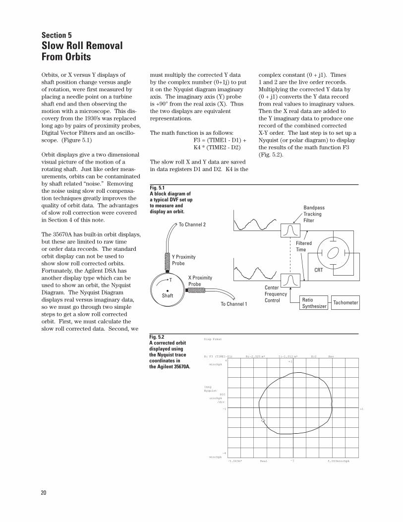
Orbits, or X versus Y displays of shaft position change versus angle of rotation, were first measured byplacing a needle point on a turbineshaft end and then observing themotion with a microscope. This dis-covery from the 1930’s was replacedlong ago by pairs of proximity probes,Digital Vector Filters and an oscillo-scope. (Figure 5.1)

Orbit displays give a two dimensionalvisual picture of the motion of arotating shaft. Just like order meas-urements, orbits can be contaminatedby shaft related “noise.” Removingthe noise using slow roll compensa-tion techniques greatly improves thequality of orbit data. The advantagesof slow roll correction were coveredin Section 4 of this note.

The 35670A has built-in orbit displays,but these are limited to raw time or order data records. The standardorbit display can not be used to show slow roll corrected orbits.Fortunately, the Agilent DSA hasanother display type which can beused to show an orbit, the NyquistDiagram. The Nyquist Diagram displays real versus imaginary data,so we must go through two simplesteps to get a slow roll correctedorbit. First, we must calculate theslow roll corrected data. Second, we

must multiply the corrected Y data by the complex number (0+1j) to putit on the Nyquist diagram imaginaryaxis. The imaginary axis (Y) probe is +90° from the real axis (X). Thusthe two displays are equivalent representations.

The math function is as follows:F3 = (TIME1 - D1) + K4 * (TIME2 - D2)

The slow roll X and Y data are savedin data registers D1 and D2. K4 is the

complex constant (0 + j1). Times 1 and 2 are the live order records.Multiplying the corrected Y data by (0 + j1) converts the Y data recordfrom real values to imaginary values.Then the X real data are added to the Y imaginary data to produce onerecord of the combined corrected X-Y order. The last step is to set up aNyquist (or polar diagram) to displaythe results of the math function F3(Fig. 5.2).

Section 5Slow Roll Removal From Orbits

T

To Channel 2

To Channel 1

Y ProximityProbe

X ProximityProbe

BandpassTrackingFilter

CenterFrequencyControl Ratio

SynthesizerTachometer

CRT

FilteredTime

Shaft

Fig. 5.1 A block diagram of a typical DVF set up to measure and display an orbit.

Fig. 5.2 A corrected orbit displayed using the Nyquist trace coordinates in the Agilent 35670A.

+j

-j

+1-1

B: F3 (TIME1-D1) X:0 RevR:-2.325 m* I:-1.012 m*

Real-5.063m* 5.063minchpk

4minchpk

-4minchpk

ImagNyquist

800uinchpk

/div

Disp Frmat

21

Example: Slow Roll Removal From Orbits

The example of slow roll removalfrom orbits uses the math and timecapture files from the example inSection 4 above. The X-Y orderrecords are combined into one datarecord for display. The standard orbitdisplay is selected with the ORBIT 2/1under the Meas Data key. The orbitdisplay works with time records inthe FFT mode or order records in the order analysis mode. To display slow roll corrected orbits, we make use of a math function tocombine the X-Y data and use theNyquist Diagram display coordinatesto view the results. As in the lastexample, the X-Y slow roll is mea-sured at 300 RPM and saved in dataregisters D1 and D2. The math func-tion takes the current order recordfor each probe and subtracts the slowroll correction. The Y axis data ismultiplied by (0 + 1j) to move it tothe imaginary axis. The X and Y dataare then combined to make a com-plex number (real + imaginary) pair.

Verify Data Setup

If the DSA has not been powereddown since the completion of theexample in Section 4, then the timecapture and math files should still bein memory. You can check by view-ing the time capture buffer and theanalysis portion of the 35670A. Todisplay the time capture buffer, press:

Active → AB → Meas Data →ALL CHANNELS → CAPTURE CHANNEL* Disp Format → UPPER/LOWER → Scale →AUTOSCALE ON OFF → ON → OFF

If the runup data do not appear onthe screen, then the time capture,state, and math records of the Section4 example will need to be recalled.To verify the math, press:


and compare F3 in the DSA to:F3 = (TIME1 - D1) + K4*(TIME2 - D2)K4 = 0.0000 + j

1.0000

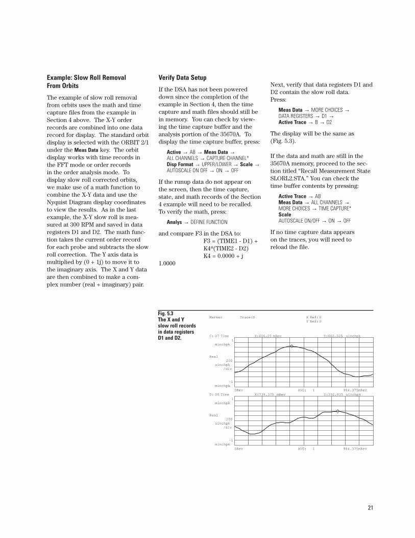
Next, verify that data registers D1 andD2 contain the slow roll data. Press:

Meas Data → MORE CHOICES →DATA REGISTERS → D1 →Active Trace → B → D2

The display will be the same as (Fig. 5.3).

If the data and math are still in the35670A memory, proceed to the sec-tion titled “Recall Measurement StateSLORL2.STA.” You can check thetime buffer contents by pressing:

Active Trace → ABMeas Data → ALL CHANNELS →MORE CHOICES → TIME CAPTURE*ScaleAUTOSCALE ON/OFF → ON → OFF

If no time capture data appears on the traces, you will need toreload the file.

Fig. 5.3 The X and Y slow roll records in data registers D1 and D2.

Marker Trace:D X Ref: 0Y Ref: 0


C: D7 Time X:406.25 mRev Y:662.325 uinchpk1

minchpk

-1minchpk

Real200

uinchpk/div

X:734.375 mRev Y:392.435 uinchpkD: D8 Time1

minchpk

-1minchpk

Real200

uinchpk/div


22

Recalling Data

Insert the disk “Agilent 35670A RotorDynamics Measurements Techniques”into the analyzer.Press:





ENTER


Rotate the marker knob to highlightthe file “SLOROL.MTH” and thenpress:


Verify that the prompt at the top ofthe analyzer screen shows“RECALL MATH = SLOROL.MTH”. Press:

ENTER


RtnRECALL STATE

Verify that the prompt at the top ofthe analyzer screen shows“RECALL STATE = SLORL1.STA”.Press:


The tach readout at the top of thescreen will increment up to approxi-mately 300 RPM and the X and Y slowroll proximity probes waveforms willappear in the A and B traces with themarkers on their respective peaks.

Now save the X-Y slow roll data inregisters D1 and D2.Press:

Active Trace → A Save Recall → SAVE DATA →SAVE TRACE → INTO D1Active Trace → B SAVE TRACE → INTO D2

Recall Measurement StateSLORL2.STA

Press:

Save/Recall → CATALOG ON OFF → ON

and rotate the marker knob to high-light the file “SLORL2.STA”. Press:

RECALL STATE

and verify “RECALL STATE =SLORL2.STA,” and then press:

ENTERDisp Format StartScale → AUTOSCALE → ON / OFF → ON

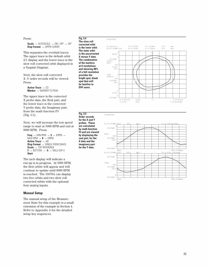
The tach display will begin to increment up. At about 3000 RPMtwo orbits will become obvious onthe display. The slow roll correctedorbit is the inner one, and the outerorbit is the raw X versus Y data. Themarker was set at 0.00 revolutions,which corresponds with the phasorleading edge, and the record length is0.984375 revolutions. The combina-tion of the markers at 0 revolutionsand the record length being about1.5% short of a full revolution pro-vides the bright spot, blank spot thatis similar to the one provided by aDVF. However, the marker must beset at 0 revolutions and not movedwhile the orbits are being displayed.The last orbit should appear near 6000 RPM and will look like (Fig. 5.4).

23

Press:

Scale → AUTOSCALE → ON / OFF → OFFDisp Format → UPPER LOWER

This separates the overlaid traces.The upper trace is the default orbit2/1 display and the lower trace is theslow roll corrected orbit displayed ina Nyquist Diagram.

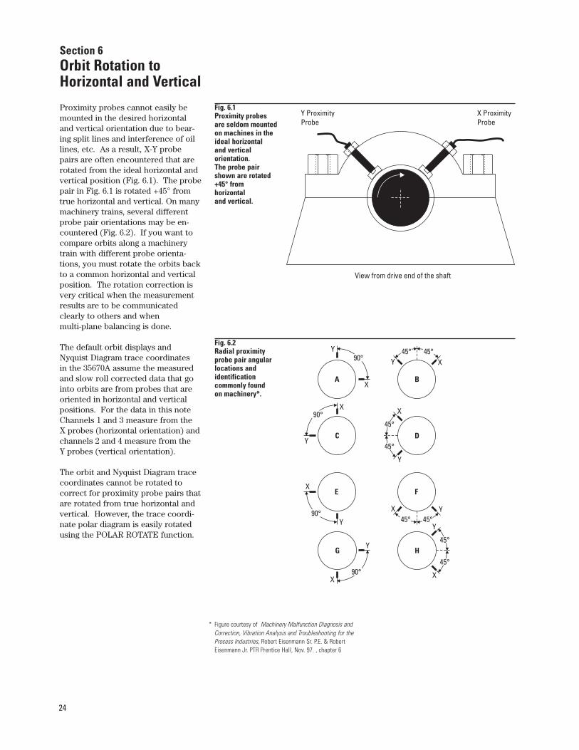
Next, the slow roll corrected X -Y order records will be viewed.Press:

Active Trace → CD Marker → MARKER TO PEAK

The upper trace is the corrected X probe data ,the Real part, and the lower trace is the corrected Y probe data, the Imaginary part,from the math function F3 (Fig. 5.5).

Next, we will increase the test speedrange to start at 5000 RPM and end at8000 RPM. Press:

Freq → MIN RPM → 5 → KRPM →MAX RPM → 8 → KRPM Active Trace → AB Disp Format → SINGLE FRONT/BACKScale → TOP REFERENCE55 → BOTTOM → -5 → MILLI-EXP-3Start

The tach display will indicate a run-up is in progress. At 5000 RPM,the first orbits will appear and willcontinue to update until 8000 RPM is reached. The 35670A can displaytwo live orbits and two slow roll corrected orbits with the optionalfour analog inputs.

Manual Setup

The manual setup of the Measure-ment State for this example is a smallextension of the example in Section 4.Refer to Appendix A for the detailedsetup key sequences.

Fig. 5.4 The slow roll corrected orbit is the inner orbit. The outer orbit is the uncorrected X versus Y data. The combination of the markers at 0 revolutions and showing 98% of a full revolution provides the bright spot, blank spot that will be familiar to DVF users.

+j

-j

+-1

Time1-5.517minch 5.517minch

A: Orbit2/1 T:0 RevX:-2.770m* Y:-1.238m*

4minch

-4minch

Time 2Real

800uinch

/div

X:0 RevR:-2.325m* I:-1.012m*B: F3 (TIME1-D1)


4minchpk

-4minchpk

ImagNyquist

800uinchpk

/div

Disp Frmat

Fig. 5.5 Order records for the X and Y probes. These are calculated by math function F3 and are viewed by displaying the real part, for the X data and the imaginary part for the Y data.

0Rev 984.375mRev

A: F3 (TIME1-D1) X:0 Rev Y:-2.325 minchpk4

minchpk

-4minchpk

Real800

uinchpk/div

X:0 Rev Y:-1.0125 minchpkB: F3 (TIME1-D1)4

minchpk

-4minchpk

Imag800

uinchpk/div

0Rev 984.375mRev

Disp Frmat

24

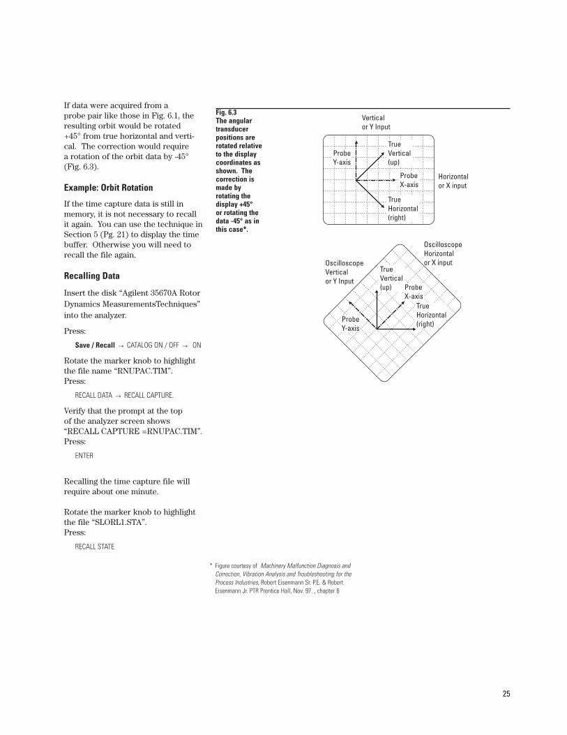
Proximity probes cannot easily bemounted in the desired horizontaland vertical orientation due to bear-ing split lines and interference of oillines, etc. As a result, X-Y probe pairs are often encountered that arerotated from the ideal horizontal andvertical position (Fig. 6.1). The probepair in Fig. 6.1 is rotated +45° fromtrue horizontal and vertical. On manymachinery trains, several differentprobe pair orientations may be en-countered (Fig. 6.2). If you want tocompare orbits along a machinerytrain with different probe orienta-tions, you must rotate the orbits backto a common horizontal and verticalposition. The rotation correction isvery critical when the measurement results are to be communicated clearly to others and when multi-plane balancing is done.

The default orbit displays and Nyquist Diagram trace coordinates in the 35670A assume the measuredand slow roll corrected data that gointo orbits are from probes that areoriented in horizontal and vertical positions. For the data in this noteChannels 1 and 3 measure from the X probes (horizontal orientation) andchannels 2 and 4 measure from the Y probes (vertical orientation).

The orbit and Nyquist Diagram tracecoordinates cannot be rotated to correct for proximity probe pairs thatare rotated from true horizontal andvertical. However, the trace coordi-nate polar diagram is easily rotatedusing the POLAR ROTATE function.

Section 6 Orbit Rotation to Horizontal and Vertical

View from drive end of the shaft

Y ProximityProbe

X ProximityProbe

E F

90°45° 45°

X

Y

X Y

G H

90°45°

45°

XX

Y

Y

A B

90°45°45°

X

Y

XY

C D

90°45°

45°

XX

Y

Y

Fig. 6.2 Radial proximity probe pair angular locations and identification commonly found on machinery*.

Fig. 6.1 Proximity probes are seldom mounted on machines in the ideal horizontal and vertical orientation. The probe pair shown are rotated +45° from horizontal and vertical.

* Figure courtesy of Machinery Malfunction Diagnosis andCorrection, Vibration Analysis and Troubleshooting for theProcess Industries, Robert Eisenmann Sr. P.E. & RobertEisenmann Jr. PTR Prentice Hall, Nov. 97. , chapter 6

25

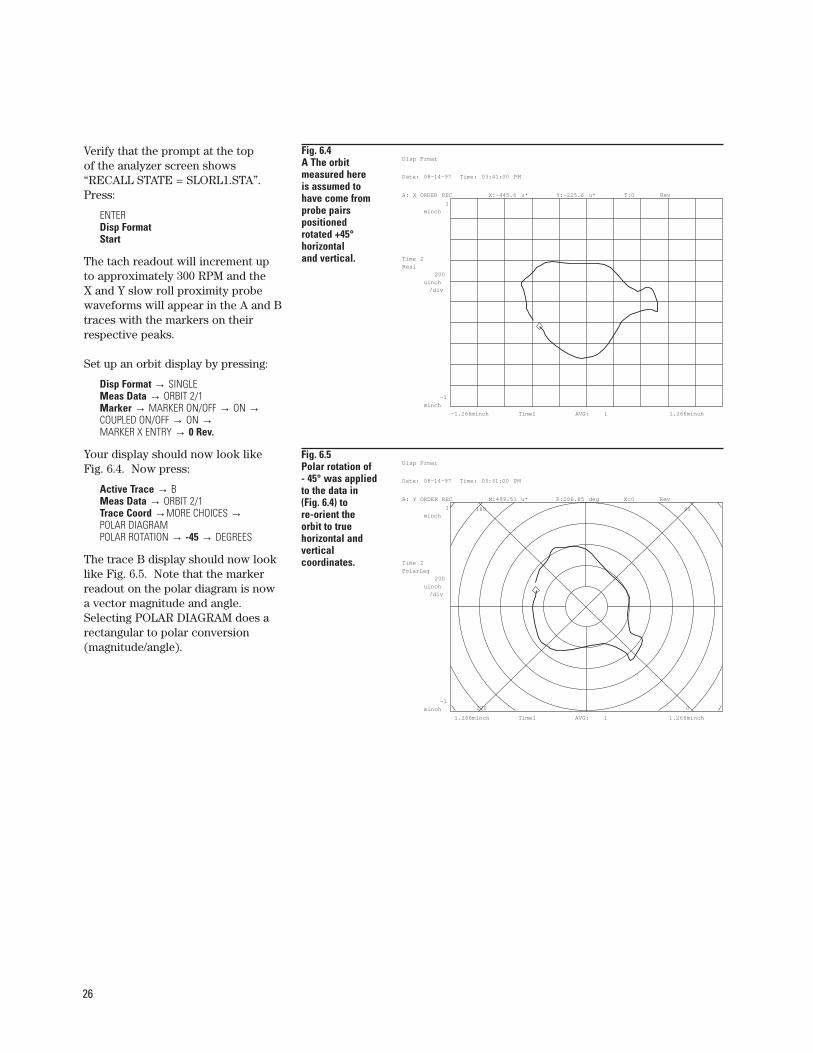
If data were acquired from a probe pair like those in Fig. 6.1, theresulting orbit would be rotated +45° from true horizontal and verti-cal. The correction would require a rotation of the orbit data by -45°(Fig. 6.3).

Example: Orbit Rotation

If the time capture data is still inmemory, it is not necessary to recallit again. You can use the technique inSection 5 (Pg. 21) to display the timebuffer. Otherwise you will need to recall the file again.

Recalling Data

Insert the disk “Agilent 35670A RotorDynamics MeasurementsTechniques”into the analyzer.

Press:





ENTER



RECALL STATE

Fig. 6.3 The angular transducer positions are rotated relative to the display coordinates as shown. The correction is made by rotating the display +45° or rotating the data -45° as in this case*.

Verticalor Y Input

OscilloscopeVerticalor Y Input

Horizontalor X input

OscilloscopeHorizontalor X input

ProbeY-axis

ProbeY-axis

TrueVertical(up)

TrueVertical(up)

ProbeX-axis

ProbeX-axis

TrueHorizontal(right)

TrueHorizontal(right)

* Figure courtesy of Machinery Malfunction Diagnosis andCorrection, Vibration Analysis and Troubleshooting for theProcess Industries, Robert Eisenmann Sr. P.E. & RobertEisenmann Jr. PTR Prentice Hall, Nov. 97. , chapter 6

26

Verify that the prompt at the top of the analyzer screen shows“RECALL STATE = SLORL1.STA”.Press:


The tach readout will increment up to approximately 300 RPM and the X and Y slow roll proximity probewaveforms will appear in the A and Btraces with the markers on theirrespective peaks.

Set up an orbit display by pressing:

Disp Format → SINGLEMeas Data → ORBIT 2/1 Marker → MARKER ON/OFF → ON →COUPLED ON/OFF → ON →MARKER X ENTRY → 0 Rev.

Your display should now look likeFig. 6.4. Now press:

Active Trace → BMeas Data → ORBIT 2/1Trace Coord →MORE CHOICES →POLAR DIAGRAM POLAR ROTATION → -45 → DEGREES

The trace B display should now looklike Fig. 6.5. Note that the markerreadout on the polar diagram is nowa vector magnitude and angle. Selecting POLAR DIAGRAM does arectangular to polar conversion (magnitude/angle).

Fig. 6.4 A The orbit measured here is assumed to have come from probe pairs positioned rotated +45° horizontal and vertical.

A: X ORDER REC T:0 RevX:-445.6 u* Y:-225.6 u*


1

minch

-1

minch

Time 2

Real

200

uinch

/div

Disp Frmat

Date: 08-14-97 Time: 03:41:00 PM

Fig. 6.5Polar rotation of - 45° was applied to the data in (Fig. 6.4) to re-orient the orbit to true horizontal and vertical coordinates.

0

180

270

90

B: Y ORDER REC X:0 RevM:499.51 u* P:206.85 deg


1

minch

-1

minch

Time 2

PolarLag

200

uinch

/div

Disp Frmat

Date: 08-14-97 Time: 03:41:00 PM

27

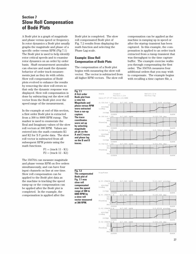
A Bodé plot is a graph of magnitudeand phase versus speed or frequency.In rotor dynamics a Bodé plot usuallygraphs the magnitude and phase of aspecific order versus RPM (Fig 7.1)The Bodé plot is used to help identifyrotor critical speeds and to examinerotor dynamics on an order by orderbasis. Shaft measurement anomaliescan obscure and mask the dynamicbehavior of order track measure-ments just as they do with orbits.Slow roll compensation of Bodé plots evolved to enhance the resultsby removing the slow roll errors sothat only the dynamic response wasdisplayed. Slow roll compensation isdone by subtracting out the slow rollvector from the Bodé plot over thespeed range of the measurement.

In the example at end of this section,a first order Bodé plot is extractedfrom a 300 to 8000 RPM runup. Themarker is used to enumerate the Real and Imaginary values of the slowroll vectors at 300 RPM. Values areentered into the math constants K1and K2 for X-Y probe data. The slowroll vector is subtracted from all subsequent RPM points using themath functions.

F1 = (track 11 - K1)F2 = (track 12 - K2)

The 35670A can measure magnitudeand phase versus RPM on five orderssimultaneously, and can have four input channels on line at one time.Slow roll compensation can beapplied to the Bodé plot data as the machine is tracking the speedramp-up or the compensation can be applied after the Bodé plot is completed. In the example, the compensation is applied after the

Bodé plot is completed. The slow roll compensated Bodé plot of Fig. 7.2 results from displaying themath function and selecting thePhase Lag scale.

Example: Slow Roll Compensation of Bodé Plots

The compensation of a Bodé plotbegins with measuring the slow rollvector. The vector is subtracted fromall higher RPM vectors. The slow roll

compensation can be applied as themachine is ramping up in speed or after the startup transient has beencaptured. In this example, the com-pensation is applied to an order trackextracted from a runup transient thatwas throughput to the time capturebuffer. The example exercise walksyou through compensating the first order. The 35670A measures fouradditional orders that you may wishto compensate. The example beginswith recalling a time capture file, a

Fig. 7.1 A first order Bodé plot from a rotor kit. Magnitude and phase versus RPM were extracted from a run-up capture. The trace coordinates were set up by selecting magnitude pk-pk on the A and C traces and phase lag on the B and D traces.

300RPM 8kRPM

A: CH1 Ord 1.00 X:7.965 kRPM Y:11.0266 minchpp12

minchpp

0inchpp

LinMag

X:7.965 kRPM Y:193.768 deg

300RPM 8kRPM

B: CH1 Ord 1.00360deg

0deg

PhaseLag

Scale Trace:C Ref Lvl: 12 mPer Div: 1.2 m Ref Pos: Top

Date:07-07-97 Time:11:10:00PM

300RPM 8kRPM

X:7.965 kRPM Y:9.79848 minchppC: CH2 Ord 1.0012

minchpp

0inchpp

LinMag

X:7.965 kRPM Y:301.952 degD: CH2 Ord 1.00360deg

0deg

PhaseLag

300RPM 8kRPM

Fig. 7.2 The compensated Bodé plot of Fig. 7.1 was slow roll compensated over the speed range of 300 to 6000 RPM by a slow roll vector measured at 300 RPM.

300RPM 8kRPM

A: F1 (TRACK11-K X:7.965 kRPM Y:10.1827 minchpp12

minchpp

0inchpp

LinMag

X:7.965 kRPM Y:199.068 deg

300RPM 8kRPM

B: F1 (TRACK11-K360deg

0deg

PhaseLag

Disp Frmat

300RPM 8kRPM

X:7.965 kRPM Y:9.45328 minchppC: F2 (TRACK12-K12

minchpp

0inchpp

LinMag

X:7.965 kRPM Y:306.154 degD: F2 (TRACK12-K360deg

0deg

PhaseLag

300RPM 8kRPM

Section 7Slow Roll Compensation of Bodé Plots

28

measurement state, and a math func-tion. You are walked through thesteps to measure, extract, and enterthe slow roll vector into the mathconstants and view the compensatedresults. Next, the display is set upmanually to compare the measuredand compensated Bodé plots.

Recalling the Setup

Note: If the time capture data is still inmemory, it is not necessary to recall itagain. You can use the technique inSection 5 (Pg. 21) to check the contents of the time buffer. You will need to recallthe state and math files for this section.

Insert the disk “Agilent 35670A RotorDynamics Measurements Techniques”into the analyzer. Press:

Save / Recall →→ CATALOG ON / OFF -> ON



Verify that the prompt at the top ofthe analyzer screen shows “RECALLCAPTURE = RNUPAC.TIM”.Press:

ENTER


Rotate the marker knob to highlightthe file “BODE.STA”. Press:

RtnRECALL STATEENTER

Rotate the marker knob to highlightthe file “BODE.MTH” and then press:


Verify that the prompt at the top of the analyzer screen shows “RECALL MATH = BODE.MTH”. Press:


to measure the Bodé plots for orders 1 through 5 on the X and Y probes.

As the measurement proceeds, thetracking markers will read out eachmeasurement point on all four traces(Fig. 7.1). The A and C traces are thelinear magnitudes in mils PP. The Band D traces are order 1 phase for theX-Y probes.

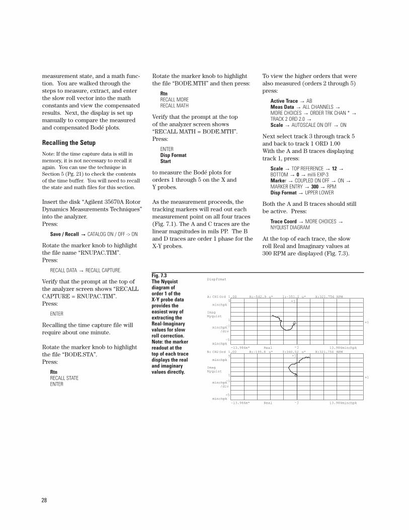
To view the higher orders that werealso measured (orders 2 through 5)press:

Active Trace → AB Meas Data → ALL CHANNELS →MORE CHOICES → ORDER TRK CHAN * →TRACK 2 ORD 2.0 →Scale → AUTOSCALE ON OFF → ON

Next select track 3 through track 5and back to track 1 ORD 1.00With the A and B traces displayingtrack 1, press:

Scale → TOP REFERENCE → 12 →BOTTOM → 0 → milli EXP-3 Marker → COUPLED ON OFF → ON →MARKER ENTRY → 300 → RPM Disp Format → UPPER LOWER

Both the A and B traces should stillbe active. Press:

Trace Coord → MORE CHOICES →NYQUIST DIAGRAM

At the top of each trace, the slow roll Real and Imaginary values at 300 RPM are displayed (Fig. 7.3).

Fig. 7.3 The Nyquist diagram of order 1 of the X-Y probe data provides the easiest way of extracting the Real-Imaginary values for slow roll correction. Note: the marker readout at the top of each trace displays the realand imaginaryvalues directly.

+j

-j

+1-1

+j

-j

+1-1


A: CH1 Ord 1.00 X:321.756 RPMR:-542.9 u* I:-351.2 u*5

minchpk

-5minchpk

ImagNyquist

1

minchpk/div

X:321.756 RPMR:-195.8 u* I:340.52 u*B: CH2 Ord 1.005

minchpk

-5minchpk

ImagNyquist

1

minchpk/div


DispFrmat

29

Copy the values in the space provided. (Be sure the marker is at300 RPM.)A: CH1 ORD1 R: ______________EXP __________I: ______________EXP __________X: 300 RPMB: CH2 ORD2 R: ______________EXP __________I: ______________EXP __________X: 300 RPM

The Real and Imaginary values will beentered into the waveform math con-stants K1 for the X probe and K2 forthe first order Y probe data.F1 = (TRACK11 - K1)F2 = (TRACK12 - K2)Press:

Analysis → DEFINE CONSTANT K1-K5 → DEFINE K1 →

Using the numeric keypad enter thereal and imaginary numbers.Real:

_________ EXP ____ → +J →+/– → – →________ EXP __DEFINE K2 →ENTER REAL & IMAG. PARTS+/– → _______ EXP ___ → +J →+/– → __________ EXP ___

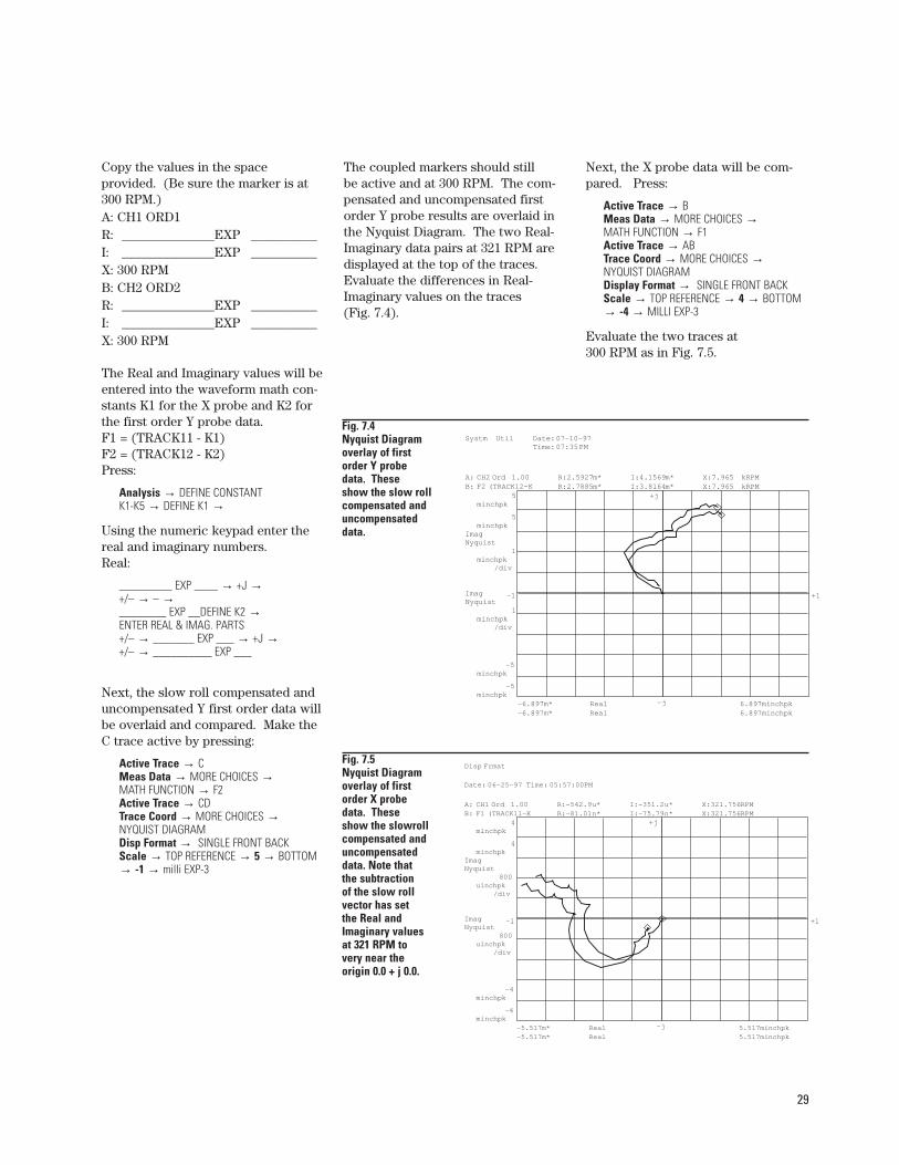
Next, the slow roll compensated anduncompensated Y first order data willbe overlaid and compared. Make theC trace active by pressing:

Active Trace → C Meas Data → MORE CHOICES →MATH FUNCTION → F2 Active Trace → CD Trace Coord → MORE CHOICES →NYQUIST DIAGRAM Disp Format → SINGLE FRONT BACK Scale → TOP REFERENCE → 5 → BOTTOM→ -1 → milli EXP-3

The coupled markers should still be active and at 300 RPM. The com-pensated and uncompensated firstorder Y probe results are overlaid inthe Nyquist Diagram. The two Real-Imaginary data pairs at 321 RPM aredisplayed at the top of the traces.Evaluate the differences in Real-Imaginary values on the traces (Fig. 7.4).

Next, the X probe data will be com-pared. Press:

Active Trace → B Meas Data → MORE CHOICES →MATH FUNCTION → F1 Active Trace → AB Trace Coord → MORE CHOICES →NYQUIST DIAGRAMDisplay Format → SINGLE FRONT BACKScale → TOP REFERENCE → 4 → BOTTOM→ -4 → MILLI EXP-3

Evaluate the two traces at 300 RPM as in Fig. 7.5.

+j

-j

+1-1


A: CH1 Ord 1.00 X:321.756RPMR:-542.9u* I:-351.2u*

4minchpk

-4minchpk

ImagNyquist

800uinchpk

/div

X:321.756RPMR:-81.01n* I:-75.79n*B: F1 (TRACK11-K


4minchpk

-4minchpk

ImagNyquist

800uinchpk

/div

Disp Frmat

Date: 06-25-97 Time: 05:57:00PM

Fig. 7.5 Nyquist Diagramoverlay of firstorder X probedata. Theseshow the slowroll compensated and uncompensateddata. Note that the subtraction of the slow roll vector has set the Real and Imaginary values at 321 RPM to very near the origin 0.0 + j 0.0.

Fig. 7.4 Nyquist Diagramoverlay of firstorder Y probedata. Theseshow the slow roll compensated and uncompensateddata.

+j

-j

+1-1


A: CH2 Ord 1.00 X:7.965 kRPMR:2.5927m* I:4.1569m*

5minchpk

-5minchpk

ImagNyquist

1minchpk

/div

X:7.965 kRPMR:2.7885m* I:3.8164m*B: F2 (TRACK12-K


5minchpk

-5minchpk

ImagNyquist

1minchpk

/div

Systm Util Date: 07-10-97Time: 07:35 PM

30

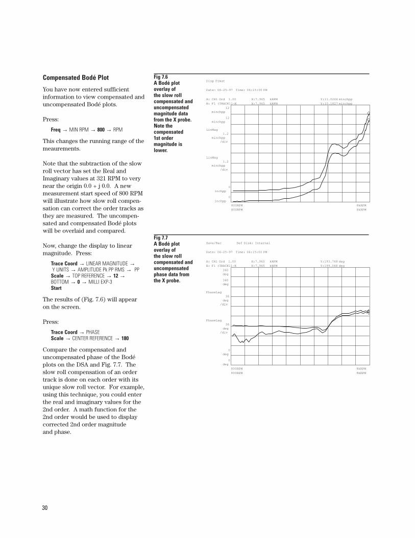
Compensated Bodé Plot

You have now entered sufficientinformation to view compensated anduncompensated Bodé plots.

Press:

Freq → MIN RPM → 800 → RPM

This changes the running range of themeaurements.

Note that the subtraction of the slowroll vector has set the Real andImaginary values at 321 RPM to verynear the origin 0.0 + j 0.0. A newmeasurement start speed of 800 RPMwill illustrate how slow roll compen-sation can correct the order tracks asthey are measured. The uncompen-sated and compensated Bodé plotswill be overlaid and compared.

Now, change the display to linearmagnitude. Press:

Trace Coord → LINEAR MAGNITUDE →Y UNITS → AMPLITUDE Pk PP RMS → PP

Scale → TOP REFERENCE → 12 →BOTTOM → 0 → MILLI EXP-3Start

The results of (Fig. 7.6) will appearon the screen.

Press:

Trace Coord → PHASE Scale → CENTER REFERENCE → 180

Compare the compensated and uncompensated phase of the Bodéplots on the DSA and Fig. 7.7. Theslow roll compensation of an ordertrack is done on each order with itsunique slow roll vector. For example,using this technique, you could enterthe real and imaginary values for the2nd order. A math function for the2nd order would be used to displaycorrected 2nd order magnitude and phase.

Fig 7.7 A Bodé plot overlay of the slow roll compensated anduncompensated phase data from the X probe.

Fig 7.6 A Bodé plot overlay of the slow roll compensated and uncompensated magnitude data from the X probe. Note the compensated 1st order magnitude is lower.

800RPM 8kRPM

A: CH1 Ord 1.00 X:7.965 kRPM Y:11.0266 minchpp

12minchpp

0inchpp

LinMag1.2

minchpp/div

X:7.965 kRPM Y:10.1827 minchppB: F1 (TRACK11-K

800RPM 8kRPM

12minchpp

0inchpp

LinMag1.2

minchpp/div

Disp Frmat

Date: 06-25-97 Time: 06:15:00 PM

800RPM 8kRPM

A: CH1 Ord 1.00 X:7.965 kRPM Y:193.768 deg

360deg

0deg

PhaseLag36

deg/div

X:7.965 kRPM Y:199.068 degB: F1 (TRACK11-K

800RPM 8kRPM

360deg

0deg

PhaseLag36

deg/div

Save/Rec Def Disk: Internal

Date: 06-25-97 Time: 06:15:00 PM

31

The measurements of shaft centerline position changes are commonlyused to investigate shifts in amachine’s shaft center of rotation.These may be due to thermal effects,load changes, oil temperature, RPM,preloads, etc. These measurementsare used to document a machine’s be-havior during startup commissioningand to monitor shaft position changesduring heat soaks. The DC gap volt-ages from X-Y proximity probes aresometimes logged along with oil andcase temperature, oil pressure andRPM. The data can then be plottedversus time, temperature, and/or RPMto document how the journal posi-tions are related to other machine variables.

The shaft center line measurementsare typically done manually, with anintegrating digital voltmeter that has5.5 digits of resolution and an accura-cy on that same order. The integrat-ing voltmeter requirement comesfrom the need to “integrate” out theAC signals, due to the dynamics ofthe rotor and AC line frequency noise.The raw voltage data are manuallyentered into a PC spreadsheet wherethe change in gap can be referencedto the at-rest gap voltages and plottedversus other variables. The proximityprobe scale factors are applied to thechange in voltage readings. The read-ings are generally taken on a one- tofour-hour time interval so the datacan be logged manually. Ideally, shaft

center line position measurementsshould be acquired on every startup.However, measuring shaft positionchanges during a fast startup tran-sient requires a high-speed dataacquisition instrument. Until recent-ly, these scanning digital integratingvoltmeters were expensive andrequired additional software to get the data to a PC spreadsheet.

The low-cost 34970A Data Logger canautomate the measurement of voltageand scaling to engineering units. Thisdata logger can be set up to captureand scale readings of gap voltages,temperatures, and pressures at user-specified time intervals. The scaledgap and other readings are easilytransferred to the PC spreadsheet via IEEE 488, or RS232 I/O using thesoftware supplied with the data log-ger. The 34970A data logger supportsa variety of scanned input cards in-cluding thermocouple, a counter/timeinterval card for RPM logging, andfour-wire resistance measurementsfor scaled strain gauge measure-ments. The data logger can scan at250 readings per second and hold50,000 time-stamped readings in its non-volatile memory. Even at250 readings per second, there arefast startup transients that this unitwould have difficulty tracking.

The 35670A DSA measures shaft center line as a standard capability ofthe computed order tracking option.An order track on order 0 for the X-Yprobes is the starting point. The zeroorder data (DC) contains the meanposition values with the higher ordervibration signals “integrated” out.The Agilent DSA can extract the cen-ter line position change versus RPMon fast runup transients, which canalso be done with the data loggerapproach for moderate speed ramprates. When the shaft center lineneeds to be monitored for longertimes such as during heat soaks, theDSA measurement arming is changedfrom RPM increment to time incre-ment. The time increment armingcan be set to range from millisecondsto hours. The measured gap valuescan come directly from the analoginputs or the transient data can becaptured and post processed.

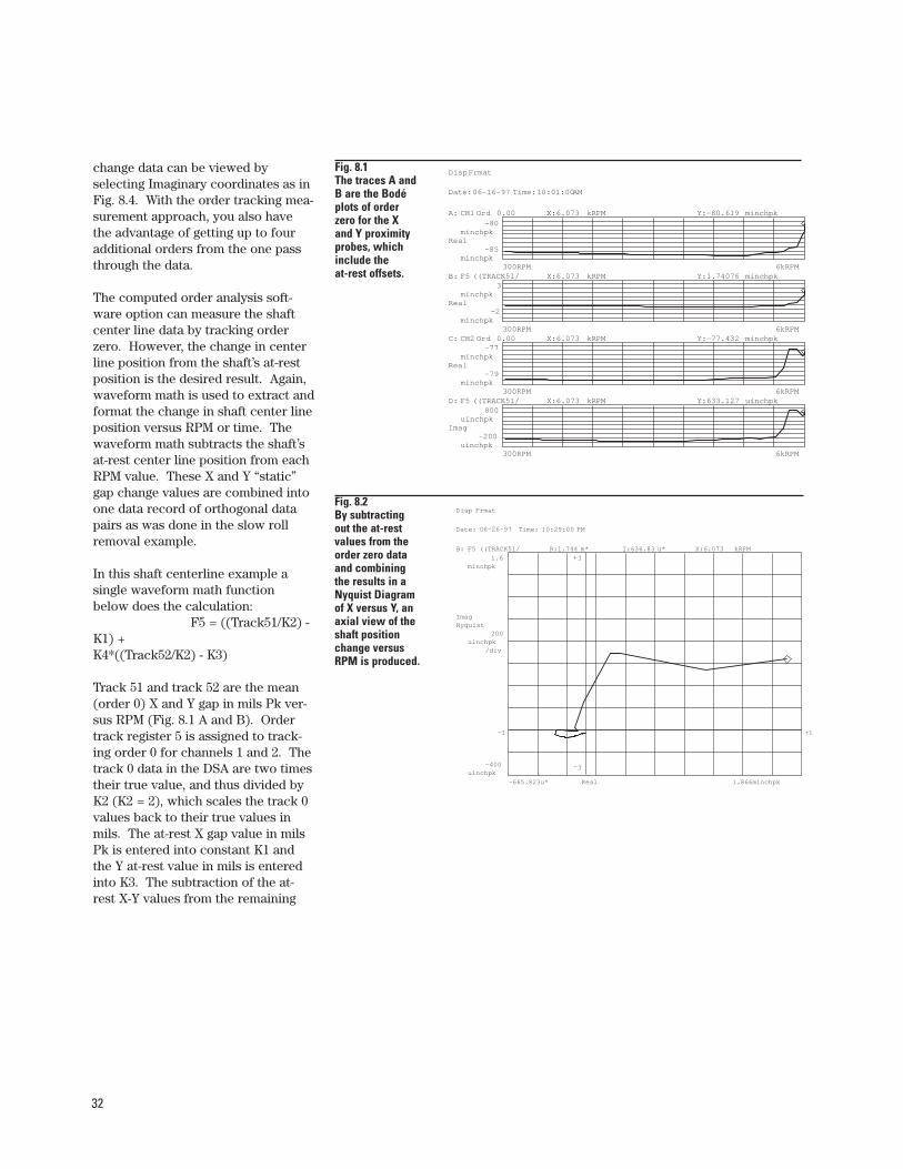
The display of the results in Fig. 8.1 A and B are the X-Y probe results.The X-Y data can be combined inNyquist Diagram or polar coordinatesto provide an axial view of the shaft’sX-Y position change as a function ofRPM (Fig. 8.2). The X data can beviewed by selecting Real trace coordi-nates as in Fig. 8.3. The Y position

Section 8 Shaft Center Line versus Speed or Time

32

change data can be viewed by selecting Imaginary coordinates as inFig. 8.4. With the order tracking mea-surement approach, you also have the advantage of getting up to fouradditional orders from the one passthrough the data.

The computed order analysis soft-ware option can measure the shaftcenter line data by tracking orderzero. However, the change in centerline position from the shaft’s at-restposition is the desired result. Again,waveform math is used to extract andformat the change in shaft center lineposition versus RPM or time. Thewaveform math subtracts the shaft’sat-rest center line position from eachRPM value. These X and Y “static”gap change values are combined intoone data record of orthogonal datapairs as was done in the slow rollremoval example.

In this shaft centerline example a single waveform math function below does the calculation:

F5 = ((Track51/K2) -K1) + K4*((Track52/K2) - K3)

Track 51 and track 52 are the mean(order 0) X and Y gap in mils Pk ver-sus RPM (Fig. 8.1 A and B). Ordertrack register 5 is assigned to track-ing order 0 for channels 1 and 2. Thetrack 0 data in the DSA are two timestheir true value, and thus divided byK2 (K2 = 2), which scales the track 0values back to their true values inmils. The at-rest X gap value in milsPk is entered into constant K1 andthe Y at-rest value in mils is enteredinto K3. The subtraction of the at-rest X-Y values from the remaining

Fig. 8.1 The traces A and B are the Bodé plots of order zero for the X and Y proximity probes, which include the at-rest offsets.

300RPM 6kRPM

A: CH1 Ord 0.00 X:6.073 kRPM Y:-80.619 minchpk-80

minchpk

-85minchpk

Real

X:6.073 kRPM Y:1.74076 minchpk

300RPM 6kRPM

B: F5 ((TRACK51/3

minchpk

-2minchpk

Real

Disp Frmat

Date:06-16-97 Time:10:01:00AM

300RPM 6kRPM

X:6.073 kRPM Y:-77.432 minchpkC: CH2 Ord 0.00-77

minchpk

-79minchpk

Real

X:6.073 kRPM Y:633.127 uinchpkD: F5 ((TRACK51/800

uinchpk

-200uinchpk

Imag

300RPM 6kRPM

Fig. 8.2 By subtracting out the at-rest values from the order zero data and combining the results in a Nyquist Diagram of X versus Y, an axial view of the shaft position change versus RPM is produced.

+j

-j

+1-1

B: F5 ((TRACK51/ X:6.073 kRPMR:1.744 m* I:636.83 u*

Real-665.823u* 1.866minchpk

1.6minchpk

-400uinchpk

ImagNyquist

200uinchpk

/div

Disp Frmat

Date: 06-26-97 Time: 10:29:00 PM

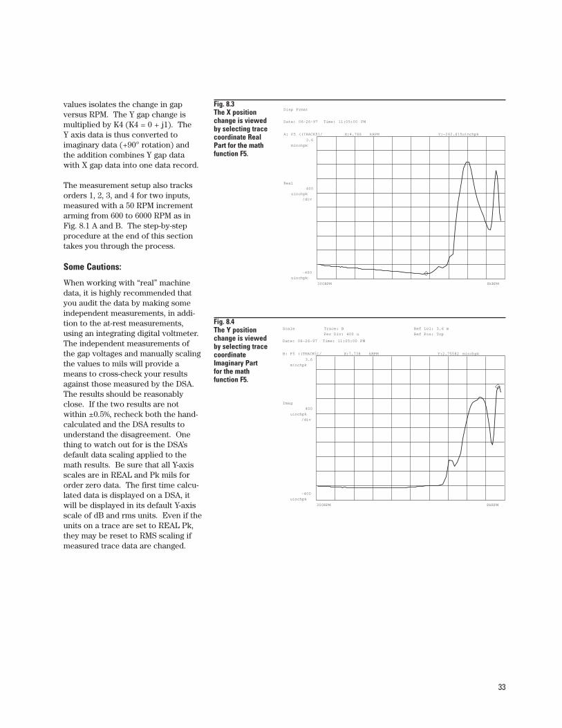
33

values isolates the change in gap versus RPM. The Y gap change ismultiplied by K4 (K4 = 0 + j1). The Y axis data is thus converted to imaginary data (+90° rotation) andthe addition combines Y gap datawith X gap data into one data record.

The measurement setup also tracksorders 1, 2, 3, and 4 for two inputs,measured with a 50 RPM incrementarming from 600 to 6000 RPM as inFig. 8.1 A and B. The step-by-stepprocedure at the end of this sectiontakes you through the process.

Some Cautions:

When working with “real” machinedata, it is highly recommended thatyou audit the data by making someindependent measurements, in addi-tion to the at-rest measurements,using an integrating digital voltmeter.The independent measurements ofthe gap voltages and manually scalingthe values to mils will provide ameans to cross-check your resultsagainst those measured by the DSA.The results should be reasonablyclose. If the two results are not within ±0.5%, recheck both the hand-calculated and the DSA results tounderstand the disagreement. Onething to watch out for is the DSA’sdefault data scaling applied to themath results. Be sure that all Y-axisscales are in REAL and Pk mils fororder zero data. The first time calcu-lated data is displayed on a DSA, itwill be displayed in its default Y-axisscale of dB and rms units. Even if theunits on a trace are set to REAL Pk,they may be reset to RMS scaling ifmeasured trace data are changed.

Fig. 8.3 The X position change is viewed by selecting trace coordinate Real Part for the math function F5.

Fig. 8.4 The Y position change is viewed by selecting trace coordinate Imaginary Part for the math function F5.

A: F5 ((TRACK51/ X:4.766 kRPM Y:-262.615uinchpk

300RPM 8kRPM

3.6

minchpk

-400

uinchpk

Real

400

uinchpk

/div

Disp Frmat

Date: 06-26-97 Time: 11:05:00 PM

B: F5 ((TRACK51/ X:7.738 kRPM Y:2.75582 minchpk

300RPM 8kRPM

3.6

minchpk

-400

uinchpk

Imag

400

uinchpk

/div

Scale Trace: B Ref Lvl: 3.6 m

Per Div: 400 u Ref Pos: Top

Date: 06-26-97 Time: 11:05:00 PM

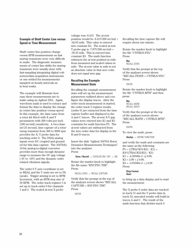
34

Example of Shaft Center Line versusSpeed or Time Measurement

Shaft center line position change versus RPM measurements on faststartup transients were very difficultto make. The diagnostic measure-ments of center line shifts for startuptransients were usually done withfast-sampling integrating digital volt-meters/data acquisition instrumentsor one settled for measurements sampled on hourly intervals as in heat soaks.

The example will illustrate how easy these measurements are to make using an Agilent DSA. Again,waveform math is used to extract and format the data to display the changein center line position versus speed.In this example, the data came from a rotor kit fitted with X and Y proximitors with 200 volts per inch(200 mv/mil) sensitivity. A two-chan-nel 25 second, time capture of a rotorrunup transient from 300 to 8000 rpmprovides the X, Y probe data fortracking order 0. The DSA’s analoginputs were DC coupled and ground-ed for this data capture. The 35670A’s16-bit analog-to-digital converter provides more than enough dynamicrange to measure the DC gap voltage(-4V to -18V) and the dynamic orderrelated vibration signals.

The order 0 Y axis coordinate is setto REAL and the Y units are set to Pk(peak). Trigger arming is set to RPMincrement, with an RPM step size of50 RPM. The order track register 5 isset up to track order 0 for channels 1 and 2. The scaled at-rest X probe

voltage was -8.41V. The at-rest position would be -8.41V/200 mv/mil = -42.05 mils. This value is entered into constant K1. The scaled at-rest Y probe gap is -7.87V/200 mv/mil = -39.35 mils. This is entered into constant K3. The math function subtracts the at-rest position in milsfrom measured and scaled values inmils. The at-rest value in mils is notan absolute value in that zero voltsdoes not equal zero gap.

Recalling the Example Measurement State

Recalling the example measurementstate will set up the measurementparameters outlined above and con-figure the display traces. After theorder track measurement is started,the order track 5 register results(order 0) are extracted from the timecapture buffer and displayed in the A and C traces. The at-rest X-Y gapvalues were entered into K1 and K3constants for math function F5. Theat-rest values are subtracted from the zero order data for display in theB and D traces.



Rotate the marker knob to highlightthe file name “RNUPDC.TIM”.Press:

RECALL DATA → RECALL CAPTURE

Verify that the prompt at the top ofthe analyzer screen shows “RECALLCAPTURE = RNUPDC.TIM”.Press:

ENTER


Rotate the marker knob to highlightthe file “CNTRLN.STA”. Press:

RtnRECALL STATE

Verify that the prompt at the top of the analyzer screen shows“RECALL STATE = CNTRLN.STA”.Press:

ENTER

Rotate the marker knob to highlightthe file “CNTRLN.MTH” and thenpress:


Verify that the prompt at the top of the analyzer screen shows“RECALL MATH = CNTRLN.MTH”. Press:

ENTER

To view the math, press:


and verify the math and constants arethe same as the following:F5 = ((TRACK51/K2) - K1) +K4*((TRACK52/K2) - K3)K1 = -4.20500e-2 +j 0.00, K2 = 2.00 + j 0.00, K3 = -3.93500e-2 + j 0.00Press:

Disp Format Start

to bring up a data display and to startthe measurement.

The X probe 0 order data are trackedin track 51 and the Y probe data intrack 52; unscaled results will build intraces A and C. The result of themath function that divides track 0

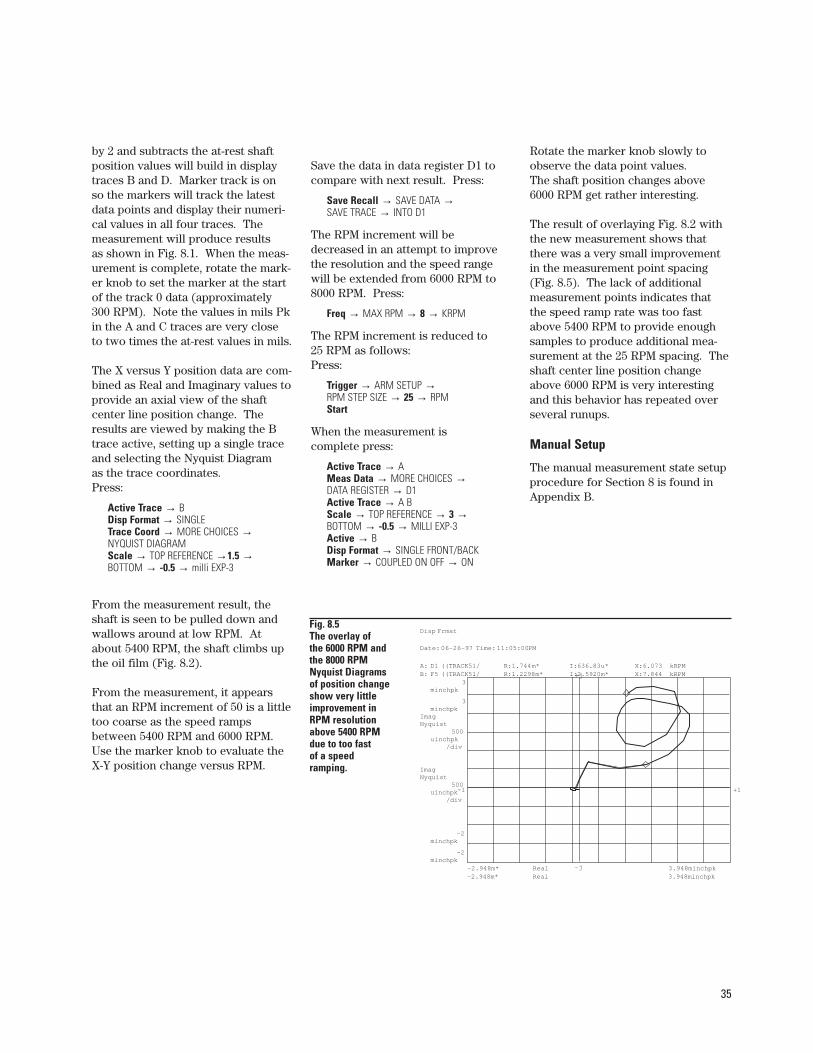
35

by 2 and subtracts the at-rest shaftposition values will build in displaytraces B and D. Marker track is on so the markers will track the latestdata points and display their numeri-cal values in all four traces. Themeasurement will produce results as shown in Fig. 8.1. When the meas-urement is complete, rotate the mark-er knob to set the marker at the startof the track 0 data (approximately300 RPM). Note the values in mils Pkin the A and C traces are very closeto two times the at-rest values in mils.

The X versus Y position data are com-bined as Real and Imaginary values toprovide an axial view of the shaftcenter line position change. Theresults are viewed by making the Btrace active, setting up a single traceand selecting the Nyquist Diagram as the trace coordinates. Press:

Active Trace → B Disp Format → SINGLE Trace Coord → MORE CHOICES →NYQUIST DIAGRAM Scale → TOP REFERENCE →1.5 →BOTTOM → -0.5 → milli EXP-3

From the measurement result, theshaft is seen to be pulled down andwallows around at low RPM. Atabout 5400 RPM, the shaft climbs upthe oil film (Fig. 8.2).

From the measurement, it appearsthat an RPM increment of 50 is a littletoo coarse as the speed rampsbetween 5400 RPM and 6000 RPM.Use the marker knob to evaluate theX-Y position change versus RPM.

Save the data in data register D1 tocompare with next result. Press:

Save Recall → SAVE DATA → SAVE TRACE → INTO D1

The RPM increment will be decreased in an attempt to improvethe resolution and the speed rangewill be extended from 6000 RPM to8000 RPM. Press:

Freq → MAX RPM → 8 → KRPM

The RPM increment is reduced to 25 RPM as follows:Press:

Trigger → ARM SETUP →RPM STEP SIZE → 25 → RPMStart

When the measurement is complete press:

Active Trace → A Meas Data → MORE CHOICES →DATA REGISTER → D1 Active Trace → A B Scale → TOP REFERENCE → 3 →BOTTOM → -0.5 → MILLI EXP-3Active → B Disp Format → SINGLE FRONT/BACKMarker → COUPLED ON OFF → ON

Rotate the marker knob slowly toobserve the data point values. The shaft position changes above6000 RPM get rather interesting.

The result of overlaying Fig. 8.2 withthe new measurement shows thatthere was a very small improvementin the measurement point spacing(Fig. 8.5). The lack of additional measurement points indicates thatthe speed ramp rate was too fastabove 5400 RPM to provide enoughsamples to produce additional mea-surement at the 25 RPM spacing. Theshaft center line position changeabove 6000 RPM is very interestingand this behavior has repeated overseveral runups.

Manual Setup

The manual measurement state setupprocedure for Section 8 is found inAppendix B.

Fig. 8.5 The overlay of the 6000 RPM and the 8000 RPM Nyquist Diagrams of position change show very little improvement in RPM resolution above 5400 RPM due to too fast of a speed ramping.

+j

-j

+1-1


A: D1 ((TRACK51/ X:6.073 kRPMR:1.744m* I:636.83u*

3minchpk

-2minchpk

ImagNyquist

500uinchpk

/div

X:7.844 kRPMR:1.2298m* I:2.5920m*B: F5 ((TRACK51/


3minchpk

-2minchpk

ImagNyquist

500uinchpk

/div

Disp Frmat

Date: 06-26-97 Time: 11:05:00PM

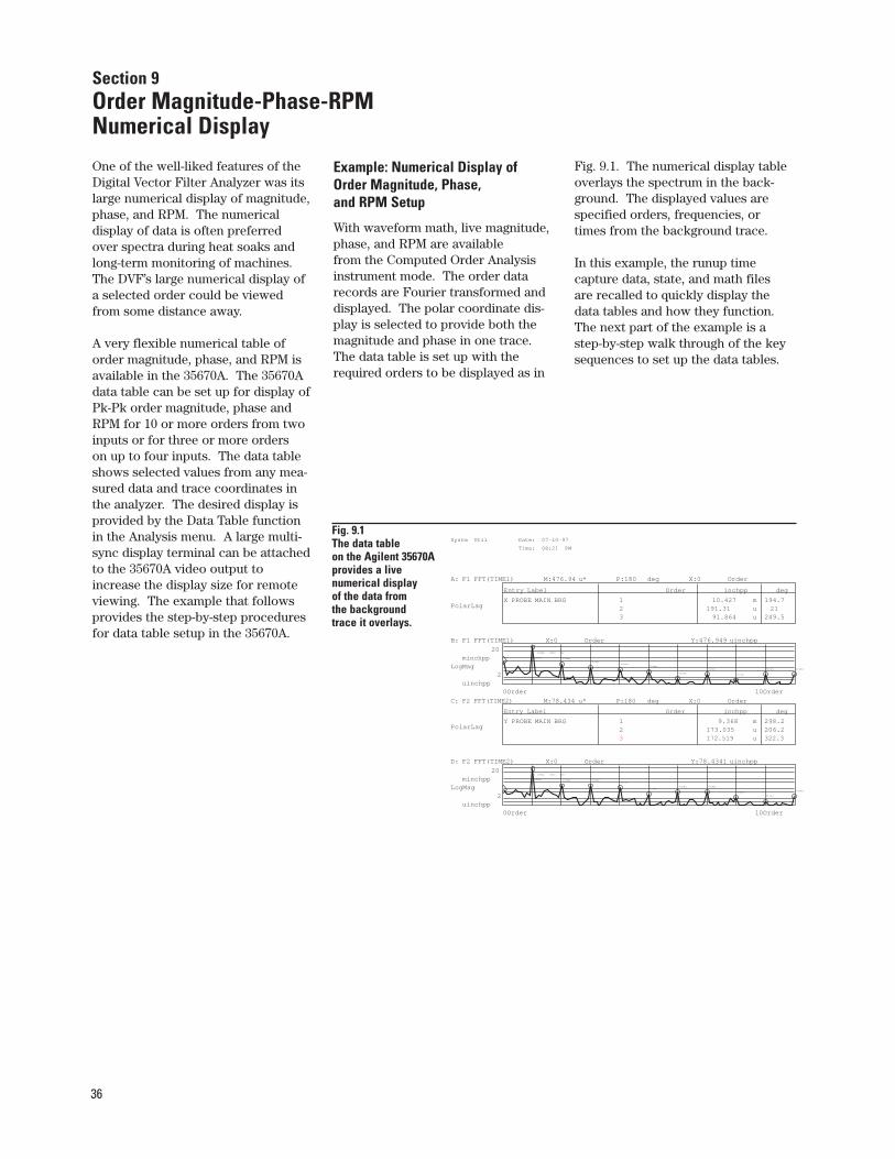
36

One of the well-liked features of theDigital Vector Filter Analyzer was itslarge numerical display of magnitude,phase, and RPM. The numerical display of data is often preferred over spectra during heat soaks andlong-term monitoring of machines.The DVF’s large numerical display ofa selected order could be viewedfrom some distance away.

A very flexible numerical table oforder magnitude, phase, and RPM isavailable in the 35670A. The 35670Adata table can be set up for display ofPk-Pk order magnitude, phase andRPM for 10 or more orders from twoinputs or for three or more orders on up to four inputs. The data tableshows selected values from any mea-sured data and trace coordinates inthe analyzer. The desired display isprovided by the Data Table functionin the Analysis menu. A large multi-sync display terminal can be attachedto the 35670A video output toincrease the display size for remoteviewing. The example that followsprovides the step-by-step proceduresfor data table setup in the 35670A.

Example: Numerical Display ofOrder Magnitude, Phase, and RPM Setup

With waveform math, live magnitude,phase, and RPM are available from the Computed Order Analysisinstrument mode. The order datarecords are Fourier transformed anddisplayed. The polar coordinate dis-play is selected to provide both the magnitude and phase in one trace.The data table is set up with the required orders to be displayed as in

Fig. 9.1. The numerical display tableoverlays the spectrum in the back-ground. The displayed values arespecified orders, frequencies, ortimes from the background trace.

In this example, the runup time capture data, state, and math filesare recalled to quickly display thedata tables and how they function.The next part of the example is astep-by-step walk through of the keysequences to set up the data tables.

Fig. 9.1 The data table on the Agilent 35670A provides a live numerical display of the data from the background trace it overlays.

Entry Label Order inchpp deg

X PROBE MAIN BRG 1 10.427 m 194.72 191.31 u 213 91.864 u 249.5

A: F1 FFT(TIME1) X:0 OrderM:476.94 u* P:180 deg

PolarLag

X:0 Order Y:476.949 uinchpp

Y PROBE MAIN BRG

1Order 2Order 3Order4Order

5Order6Order 7Order

8Order

9Order

10Order

0Order 10Order

B: F1 FFT(TIME1)

20minchpp

2uinchpp

LogMag

Systm Util Date: 07-10-97

Time: 08:21 PM


Y PROBE MAIN BRG 1 9.368 m 298.22 173.035 u 206.23 172.519 u 322.3

X:0 OrderM:78.434 u* P:180 degC: F2 FFT(TIME2)

PolarLag

X:0 Order Y:78.4341 uinchpp

X PROBE MAIN BRG

1Order 2Order

3Order4Order

5Order

6Order

7Order

8Order

9Order 10Order

D: F2 FFT(TIME2)

20minchpp

2uinchpp

LogMag

0Order 10Order

Section 9Order Magnitude-Phase-RPM Numerical Display

37

Recalling the Files





Verify that the prompt at the top ofthe analyzer screen shows “RECALLCAPTURE = RNUPAC.TIM”.Press:

ENTER


Rotate the marker knob to highlightthe file “DSPNUM.MTH” and thenpress:


Verify that the prompt at the top ofthe analyzer screen shows “RECALLMATH = DSPNUM.MTH”. Press:

ENTER

Rotate the marker knob to highlightthe file “DSPNUM.STA”. Press:

RtnRECALL STATE

Verify that the prompt at the top ofthe analyzer screen shows “RECALLSTATE = DSPNUM.STA”.Press:


The numerical values will begin toupdate in the table as the data in thespectra are updated every 60 RPM.Press:

Disp Format → UPPER LOWERStart Active Trace → CD

Measurement State Setup

The manual key strokes that wereused to set up the measurement stateon the disk are:

Preset → DO PRESET Inst Mode → ORDER ANALYSIS →TIME CAPTURE →MEASURE FROM INPUT BUFR → BUFRInput → ALL CHANNELS →XDCR UNIT CH* SETUP →XDCR UNITS ON OFF → ON →XDCR SENSITIVITY → 200 →V/EU → XDCR UNITS LABEL →MORE CHOICES → INCHFreq → MIN RPM → 300 → RPM →MAX RPM → 8 → KRPMTrigger → EXTERNAL TRIGGER →ARM SETUP → RPM STEP ARM →RPM STEP SIZE → 60 → RPM

Waveform Math

The waveform math functions F1 and F2 calculate the linear spectrafor use in the data table.

The waveform math equations for linear spectra are:

F1 = FFT (Time 1)F2 = FFT (Time 2).

If your 35670A has 4 inputs you canalso define:

F3 = FFT (Time 3)F4 = FFT (Time 4)

The key sequence is as follows:

Analysis → MATH FUNCTION →DEFINE FUNCTION → DEFINE F1 →OPERATION → FFT( → MEASURED DATA →CHANNEL 1234 → 1 → TIME1 → ) →ENTERDEFINE F2 → OPERATION → FFT ( →MEASURED DATA → CHANNEL 1234 → 2 →TIME2 → ) → ENTER

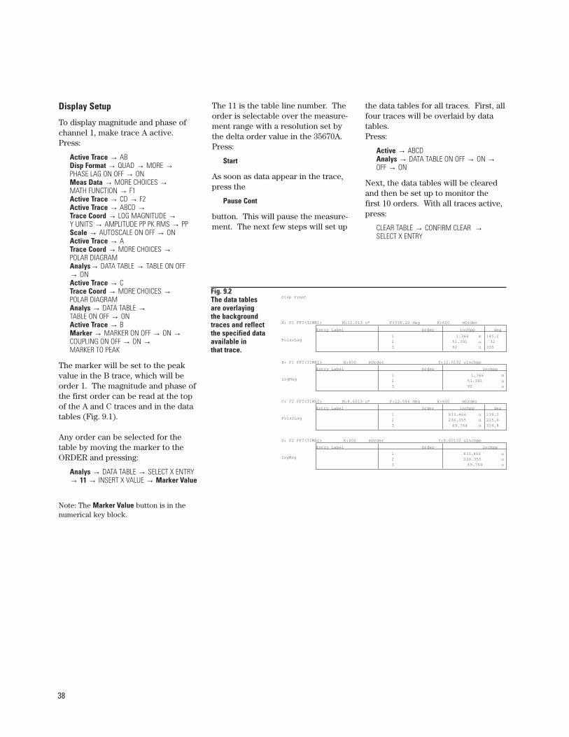
38

Display Setup

To display magnitude and phase ofchannel 1, make trace A active.Press:

Active Trace → AB Disp Format → QUAD → MORE →PHASE LAG ON OFF → ON Meas Data → MORE CHOICES →MATH FUNCTION → F1 Active Trace → CD → F2 Active Trace → ABCD →Trace Coord → LOG MAGNITUDE →Y UNITS → AMPLITUDE PP PK RMS → PPScale → AUTOSCALE ON OFF → ON Active Trace → ATrace Coord → MORE CHOICES →POLAR DIAGRAMAnalys→ DATA TABLE → TABLE ON OFF → ON Active Trace → C Trace Coord → MORE CHOICES →POLAR DIAGRAMAnalys → DATA TABLE →TABLE ON OFF → ONActive Trace → B Marker → MARKER ON OFF → ON →COUPLING ON OFF → ON →MARKER TO PEAK

The marker will be set to the peakvalue in the B trace, which will beorder 1. The magnitude and phase ofthe first order can be read at the topof the A and C traces and in the datatables (Fig. 9.1).

Any order can be selected for thetable by moving the marker to theORDER and pressing:

Analys → DATA TABLE → SELECT X ENTRY→ 11 → INSERT X VALUE → Marker Value

Note: The Marker Value button is in thenumerical key block.

The 11 is the table line number. Theorder is selectable over the measure-ment range with a resolution set bythe delta order value in the 35670A.Press:

Start

As soon as data appear in the trace,press the

Pause Cont

button. This will pause the measure-ment. The next few steps will set up

the data tables for all traces. First, allfour traces will be overlaid by datatables.Press:

Active → ABCDAnalys → DATA TABLE ON OFF → ON →OFF → ON

Next, the data tables will be clearedand then be set up to monitor thefirst 10 orders. With all traces active,press:

CLEAR TABLE → CONFIRM CLEAR →SELECT X ENTRY

Fig. 9.2 The data tables are overlaying the background traces and reflect the specified data available in that trace.


1 1.366 m 145.22 51.391 u 323 92 u 335

A: F1 FFT(TIME1) X:600 mOrderM:12.013 u* P:336.22 deg

PolarLag

X:600 mOrder Y:12.0132 uinchpp

Entry Label Order inchpp

1 1.366 m2 51.391 u3 92 u

B: F1 FFT(TIME1)

LogMag

Disp Frmat


1 833.466 u 239.22 236.355 u 225.63 69.764 u 314.8

X:600 mOrderM:8.6013 u* P:22.546 degC: F2 FFT(TIME2)

PolarLag

Entry Label Order inchpp

1 833.466 u

2 236.355 u3 69.764 u

X:600 mOrder Y:8.60132 uinchppD: F2 FFT(TIME2)

LogMag

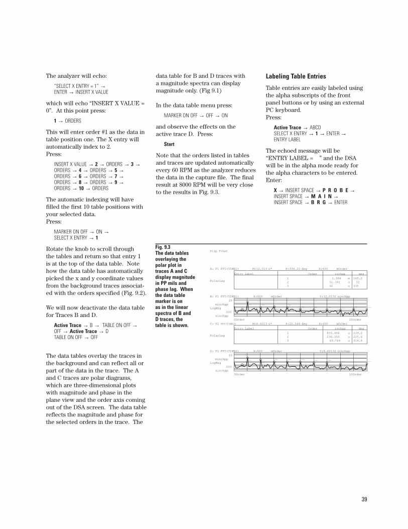
39

The analyzer will echo:

“SELECT X ENTRY = 1” →ENTER → INSERT X VALUE

which will echo “INSERT X VALUE =0”. At this point press:

1 → ORDERS

This will enter order #1 as the data intable position one. The X entry willautomatically index to 2. Press:

INSERT X VALUE → 2 → ORDERS → 3 →ORDERS → 4 → ORDERS → 5 →ORDERS → 6 → ORDERS → 7 →ORDERS → 8 → ORDERS → 9 →ORDERS → 10 → ORDERS

The automatic indexing will havefilled the first 10 table positions withyour selected data.Press:

MARKER ON OFF → ON →SELECT X ENTRY → 1

Rotate the knob to scroll through the tables and return so that entry 1is at the top of the data table. Notehow the data table has automaticallypicked the x and y coordinate valuesfrom the background traces associat-ed with the orders specified (Fig. 9.2).

We will now deactivate the data tablefor Traces B and D.

Active Trace → B → TABLE ON OFF →OFF → Active Trace → DTABLE ON OFF → OFF

The data tables overlay the traces inthe background and can reflect all orpart of the data in the trace. The Aand C traces are polar diagrams,which are three-dimensional plotswith magnitude and phase in theplane view and the order axis comingout of the DSA screen. The data tablereflects the magnitude and phase forthe selected orders in the trace. The

data table for B and D traces with a magnitude spectra can display magnitude only. (Fig 9.1)

In the data table menu press:

MARKER ON OFF → OFF → ON

and observe the effects on the active trace D. Press:

Start

Note that the orders listed in tablesand traces are updated automaticallyevery 60 RPM as the analyzer reducesthe data in the capture file. The finalresult at 8000 RPM will be very closeto the results in Fig. 9.3.

Labeling Table Entries

Table entries are easily labeled usingthe alpha subscripts of the frontpanel buttons or by using an externalPC keyboard. Press:

Active Trace → ABCD SELECT X ENTRY → 1 → ENTER →ENTRY LABEL

The echoed message will be “ENTRY LABEL = ” and the DSAwill be in the alpha mode ready forthe alpha characters to be entered.Enter:

X → INSERT SPACE → P R O B E →INSERT SPACE → M A I N →INSERT SPACE → B R G → ENTER

Fig. 9.3 The data tables overlaying the polar plot in traces A and C display magnitude in PP mils and phase lag. When the data table marker is on as in the linear spectra of B and D traces, the table is shown.


1 1.366 m 145.22 51.391 u 323 92 u 335


PolarLag


1Order

2Order

3Order 4Order 5Order6Order 7Order

8Order

9Order

10Order

0Order 10Order

B: F1 FFT(TIME1)

20minchpp

200ninchpp

LogMag

Disp Frmat


1 833.466 u 239.22 236.355 u 225.63 69.764 u 314.8

X:600 mOrderM:8.6013 u* P:22.546 degC: F2 FFT(TIME2)

PolarLag


1Order 2Order

3Order

4Order

5Order 6Order 7Order8Order

9Order 10Order

D: F2 FFT(TIME2)

20minchpp

200ninchpp

LogMag

0Order 10Order

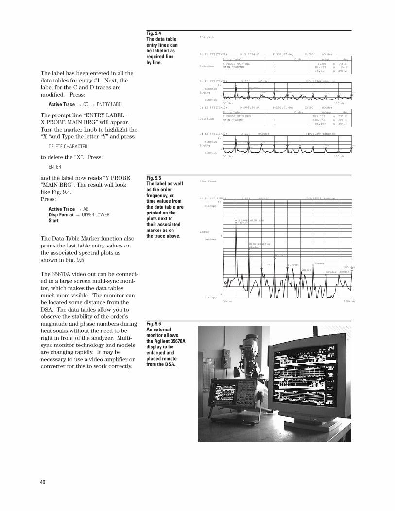
40

The label has been entered in all thedata tables for entry #1. Next, thelabel for the C and D traces are modified. Press:

Active Trace → CD → ENTRY LABEL

The prompt line “ENTRY LABEL = X PROBE MAIN BRG” will appear.Turn the marker knob to highlight the“X “and Type the letter “Y” and press:

DELETE CHARACTER

to delete the “X”. Press:

ENTER

and the label now reads “Y PROBE“MAIN BRG”. The result will look like Fig. 9.4.Press:

Active Trace → AB Disp Format → UPPER LOWERStart

The Data Table Marker function alsoprints the last table entry values onthe associated spectral plots asshown in Fig. 9.5

The 35670A video out can be connect-ed to a large screen multi-sync moni-tor, which makes the data tablesmuch more visible. The monitor canbe located some distance from theDSA. The data tables allow you toobserve the stability of the order’smagnitude and phase numbers duringheat soaks without the need to beright in front of the analyzer. Multi-sync monitor technology and modelsare changing rapidly. It may be necessary to use a video amplifier orconverter for this to work correctly.

Fig. 9.4 The data table entry lines can be labeled as required line by line.


X PROBE MAIN BRG 1 1.305 m 145.1MAIN BEARING 2 84.079 u 25.2

3 15.81 u 290.2


PolarLag


Y PROBE MAIN BRG

1Order MAIN BEARING

2Order

3Order4Order 5Order

6Order 7Order8Order

9Order

10Order

0Order 10Order

B: F1 FFT(TIME1)

10minchpp

1uinchpp

LogMag

Analysis


Y PROBE MAIN BRG 1 783.533 u 237.2MAIN BEARING 2 230.073 u 224.3

3 86.407 u 304.7

X:200 mOrderM:905.56 n* P:292.01 degC: F2 FFT(TIME2)

PolarLag

X:200 mOrder Y:905.564 ninchpp

X PROBE MAIN BRG

1Order

MAIN BEARING

2Order

3Order

4Order

5Order

6Order

7Order

8Order 9Order10Order

D: F2 FFT(TIME2)

10minchpp

1uinchpp

LogMag

0Order 10Order

Fig. 9.5 The label as well as the order, frequency, or time values from the data table are printed on the plots next to their associated marker as on the trace above.

B: F1 FFT(TIME1) X:200 mOrder Y:3.93944 uinchpp

0Order 10Order

10

minchpp

1

uinchpp

LogMag

4

decades

Disp Frmat

X PROBE MAIN BRG1Order

MAIN BEARING2Order

3Order

4Order

5Order

6Order

7Order

8Order 9Order

10Order

Fig. 9.6An externalmonitor allowsthe Agilent 35670Adisplay to beenlarged andplaced remotefrom the DSA.

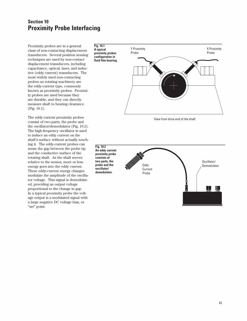
41

Proximity probes are in a generalclass of non-contacting displacementtransducers. Several position sensingtechniques are used by non-contactdisplacement transducers, includingcapacitance, optical, laser, and induc-tive (eddy current) transducers. Themost widely used non-contactingprobes on rotating machinery are the eddy-current type, commonlyknown as proximity probes. Proximi-ty probes are used because they are durable, and they can directlymeasure shaft to bearing clearance. (Fig. 10.1).

The eddy-current proximity probesconsist of two parts, the probe andthe oscillator/demodulator (Fig. 10.2).The high-frequency oscillator is usedto induce an eddy current on theshaft’s surface without actually touch-ing it. The eddy-current probes cansense the gap between the probe tipand the conductive surface of therotating shaft. As the shaft moves relative to the sensor, more or lessenergy goes into the eddy current.These eddy-current energy changesmodulate the amplitude of the oscilla-tor voltage. This signal is demodulat-ed, providing an output voltageproportional to the change in gap. In a typical proximity probe the volt-age output is a modulated signal witha large negative DC voltage bias, or “set” point.

View from drive end of the shaft

Y ProximityProbe

X ProximityProbe

Oscillator/DemodulatorEddy

CurrentProbe

Fig. 10.1 A typical proximity probes configuration in fluid film bearing.

Fig. 10.2 An eddy current proximity probe consists of two parts, the probe and the oscillator/demodulator.

Section 10Proximity Probe Interfacing

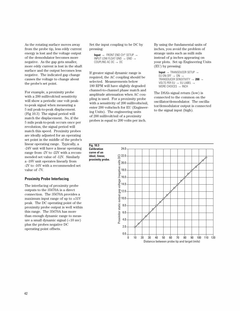
42

As the rotating surface moves awayfrom the probe tip, less eddy currentenergy is lost and the voltage outputof the demodulator becomes morenegative. As the gap gets smaller,more eddy current is lost in the shaftsurface and the output becomes lessnegative. The indicated gap changecauses the voltage to change aboutthe probe’s set point.

For example, a proximity probe with a 200 millivolt/mil sensitivity will show a periodic one volt peak-to-peak signal when measuring a 5 mil peak-to-peak displacement.(Fig 10.3) The signal period willmatch the displacement. So, if the 5 mils peak-to-peak occurs once perrevolution, the signal period willmatch this speed. Proximity probesare ideally adjusted for an operatingset point in the middle of the probe’slinear operating range. Typically, a -24V unit will have a linear operatingrange from -2V to -22V with a recom-mended set value of -12V. Similarly a -18V unit operates linearly from -2V to -16V with a recommended setvalue of -7V.

Proximity Probe Interfacing

The interfacing of proximity probeoutputs to the 35670A is a direct connection. The 35670A provides amaximum input range of up to ±31Vpeak. The DC operating point of theproximity probe output is well withinthis range. The 35670A has morethan enough dynamic range to meas-ure a small dynamic signal (<10 mv)plus the probes negative DC operating point offsets.

Set the input coupling to be DC bypressing:

Input → FRONT END CH* SETUP →INPUT LOW FLOAT GND → GND →COUPLING AC DC → DC

If greater signal dynamic range isrequired, the AC coupling should beselected. Measurements below 180 RPM will have slightly degradedchannel-to-channel phase match andamplitude attenuation when AC cou-pling is used. For a proximity probewith a sensitivity of 200 millivolts/mil,enter 200 volts/inch for EU (Engineer-ing Units). The engineering units of 200 millivolt/mil of a proximityprobes is equal to 200 volts per inch.

By using the fundamental units ofinches, you avoid the problem ofstrange units such as milli mils instead of µ inches appearing on your plots. Set up Engineering Units(EU) by pressing:

Input → TRANSDUCER SETUP →EU ON OFF → ON →TRANSDUCER SENSITIVITY → 200 →VOLTS PER EU → EU LABEL →MORE CHOICES → INCH

The DSA’s signal return (low) is connected to the common on the oscillator/demodulator. The oscilla-tor/demodulator output is connectedto the signal input (high).

Fig. 10.3 Calibration curve of an ideal, linear, proximity probe.

24.0

22.0

20.0

18.0

16.0

14.0

12.0

10.0

8.0

6.0

4.0

2.0

0.00 10 20 30 40 50 60 70 80 90 100 110 120

Prox

imito

rsta

ticou

tput

gap

volta

ge(n

egat

ive

volts

DC)

Distance between probe tip and target (mils)

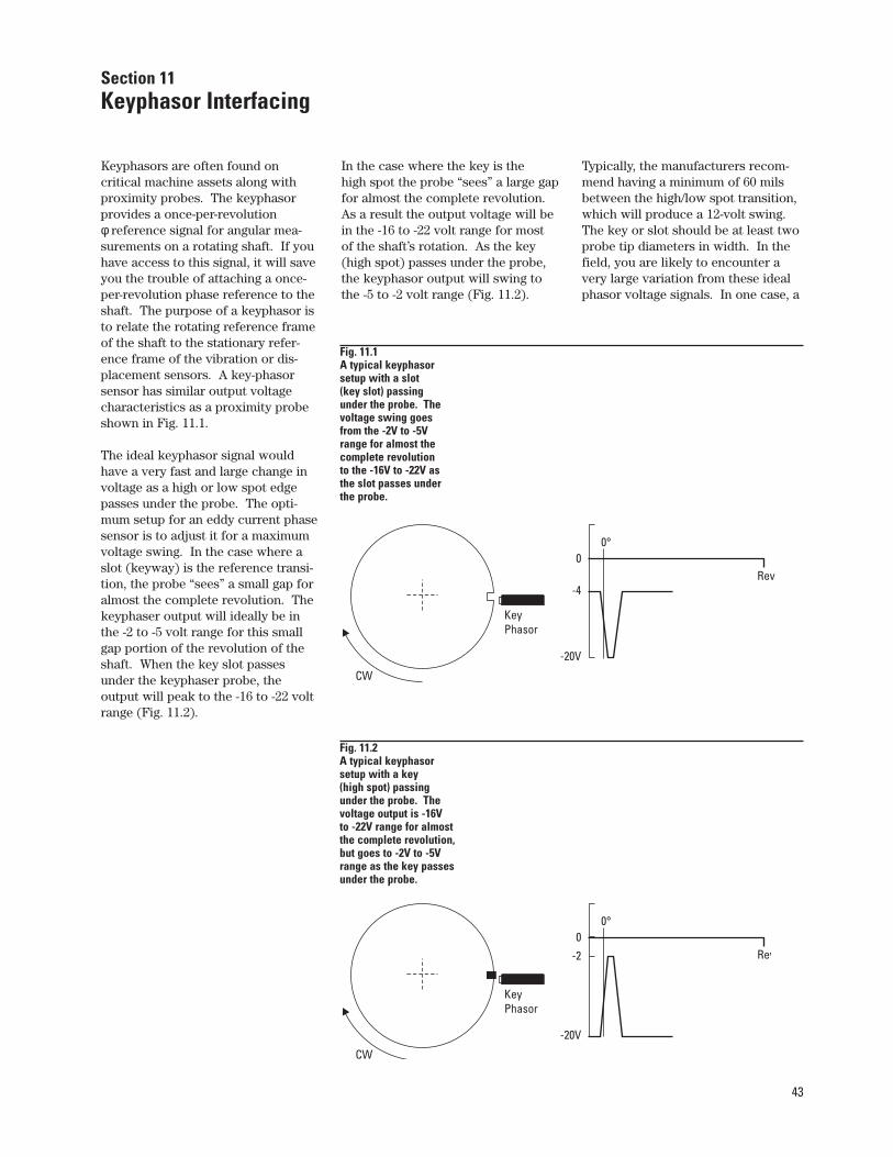
43

Keyphasors are often found on critical machine assets along withproximity probes. The keyphasorprovides a once-per-revolution φ reference signal for angular mea-surements on a rotating shaft. If youhave access to this signal, it will saveyou the trouble of attaching a once-per-revolution phase reference to theshaft. The purpose of a keyphasor isto relate the rotating reference frameof the shaft to the stationary refer-ence frame of the vibration or dis-placement sensors. A key-phasorsensor has similar output voltagecharacteristics as a proximity probeshown in Fig. 11.1.

The ideal keyphasor signal wouldhave a very fast and large change involtage as a high or low spot edgepasses under the probe. The opti-mum setup for an eddy current phasesensor is to adjust it for a maximumvoltage swing. In the case where aslot (keyway) is the reference transi-tion, the probe “sees” a small gap foralmost the complete revolution. Thekeyphaser output will ideally be inthe -2 to -5 volt range for this smallgap portion of the revolution of theshaft. When the key slot passesunder the keyphaser probe, the output will peak to the -16 to -22 voltrange (Fig. 11.2).

In the case where the key is the high spot the probe “sees” a large gapfor almost the complete revolution.As a result the output voltage will bein the -16 to -22 volt range for most of the shaft’s rotation. As the key(high spot) passes under the probe,the keyphasor output will swing to the -5 to -2 volt range (Fig. 11.2).

Typically, the manufacturers recom-mend having a minimum of 60 milsbetween the high/low spot transition,which will produce a 12-volt swing.The key or slot should be at least twoprobe tip diameters in width. In thefield, you are likely to encounter avery large variation from these idealphasor voltage signals. In one case, a

Fig. 11.1 A typical keyphasor setup with a slot (key slot) passing under the probe. The voltage swing goes from the -2V to -5V range for almost the complete revolution to the -16V to -22V as the slot passes under the probe.

CW

KeyPhasor

0

-20V

Rev-4

0°

Fig. 11.2 A typical keyphasor setup with a key (high spot) passing under the probe. The voltage output is -16V to -22V range for almost the complete revolution, but goes to -2V to -5V range as the key passes under the probe.

CW

KeyPhasor

0

-20V

Rev-2

0°

Section 11Keyphasor Interfacing

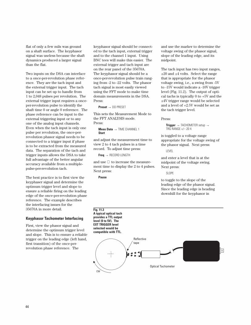
44

flat of only a few mils was ground on a shaft surface. The keyphasorsignal was useless because the shaftdynamics produced a larger signalthan the flat.

Two inputs on the DSA can interfaceto a once-per-revolution phase refer-ence. They are the tach input and the external trigger input. The tachinput can be set up to handle from 1 to 2,048 pulses per revolution. Theexternal trigger input requires a once-per-revolution pulse to identify theshaft time 0 or angle 0 reference. Thephase reference can be input to theexternal triggering input or to anyone of the analog input channels.Even when the tach input is only onepulse per revolution, the once-per-revolution phasor signal needs to beconnected to a trigger input if phaseis to be extracted from the measureddata. The separation of the tach andtrigger inputs allows the DSA to takefull advantage of the better angularaccuracy available from a multiple-pulse-per-revolution tach.

The best practice is to first view thekeyphaser signal and determine theoptimum trigger level and slope toensure a reliable firing on the leadingedge of the once-per-revolution phasereference. The example describes the interfacing issues for the 35670A in more detail.

Keyphasor Tachometer Interfacing

First, view the phasor signal anddetermine the optimum trigger leveland slope. This is to ensure a reliabletrigger on the leading edge (left hand,first transition) of the once-per-revolution phase reference. The

keyphasor signal should be connect-ed to the tach input, external triggerand to the channel 1 input. UsingBNC tees will make this easier. Theexternal trigger and tach input are on the rear panel of the 35670A. The keyphasor signal should be aonce-per-revolution pulse train rang-ing from -2 to -22 volts. The phasortach signal is most easily viewedusing the FFT mode to make time domain measurements in the DSA.Press:


This sets the Measurement Mode tothe FFT ANALYSIS mode. Press:

Meas Data → TIME CHANNEL 1 Start

and adjust the measurement time toview 2 to 4 tach pulses in a timerecord. To adjust time press:

Freq → RECORD LENGTH

and use ⇑ to increase the measure-ment time to display the 2 to 4 pulses.Next press:

Pause

and use the marker to determine thevoltage swing of the phasor signal,slope of the leading edge, and its midpoint.

The tach input has two input ranges,±20 and ±4 volts. Select the rangethat is appropriate for the phasorvoltage swing, i.e., a swing from -5Vto -15V would indicate a -10V triggerlevel (Fig. 11.2). The output of opti-cal tachs is typically 0 to +5V and the±4V trigger range would be selectedand a level of +2.5V would be set asthe tach trigger level.

Press:

Trigger → TACHOMETER setup →TRG RANGE +/– 20 4

is toggled to a voltage range appropriate for the voltage swing ofthe phasor signal. Next press:

LEVEL

and enter a level that is at the midpoint of the voltage swing. Next press:

SLOPE

to toggle to the slope of the leading edge of the phasor signal.Since the leading edge is headingdownhill for the keyphasor in

Fig. 11.3A typical optical tach provides a TTL output level (0 to 5V). The EXT TRIGGER level selected would be compatible with TTL.

CW

Reflectivetape

Optical Tachometer

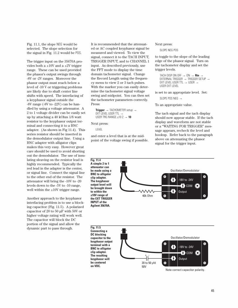
45

Fig. 11.1, the slope NEG would be selected. The slope selection for the signal in Fig. 11.2 would be POS.

The trigger input on the 35670A pro-vides both a ±10V and a ±2V triggerrange. These can be used providedthe phasor’s output swings through -8V or -2V ranges. Moreover the phasor output must reach below alevel of -10 V or triggering problemsare likely due to shaft center lineshifts with speed. The interfacing ofa keyphasor signal outside the -8V range (-8V to -22V) can be han-dled by using a voltage attenuator. A2 to 1 voltage divider can be easily setup by attaching a 40 kOhm 1/8 wattresistor to the keyphasor output ter-minal and connecting it to a BNCadapter. (As shown in Fig 11.4). This series resistor should be inserted inthe demodulator output line. Using aBNC adapter with alligator clipsmakes this very easy. However greatcare should be used to avoid shortingout the demodulator. The use of insu-lating sleaving on the resistor lead ishighly recommended. Typically thered lead in the adapter is the center,or signal line. Connect the signal lineto the other end of the resistor. Theattenuator will bring the -10V to -20levels down to the -5V to -10 range,well within the ±10V trigger range.

Another approach to the keyphasorinterfacing problem is to use a block-ing capacitor (Fig. 11.5). A polarizedcapacitor of 20 to 50 µF with 50V orhigher voltage rating will work well.The capacitor will block the DC portion of the signal and allow the dynamic part to pass through.

It is recommended that the attenuat-ed or AC coupled keyphasor signal bemeasured and viewed. To view thesignal, connect it to the TACH INPUT,TRIGGER INPUT, and to CHANNEL 1input. As described previously, usethe FFT mode to display the timedomain tachometer signal. Changethe Record Length using the frequen-cy menu to view 2 or 3 tach pulses. With the marker you can easily deter-mine the tachometer signal voltageswing and midpoint. You can then setthe tachometer parameters correctly.Press:

Trigger → TACHOMETER setup →EXT LEVEL USER TTL →USER TRG RANGE ±10 2 → 10

Next press:

LEVEL

and enter a level that is at the mid-point of the voltage swing if possible.

Next press:

SLOPE NEG POS

to toggle to the slope of the leadingedge of the phasor signal. Turn onthe tachometer display and set thetrigger levels.

TACH DISP ON OFF → ON → Rtn →EXTERNAL TRIGGER → TRIGGER SETUP →EXT LEVEL USER TTL → USER →USER EXT LEVEL

is set to an appropriate level. Set:

SLOPE POS NEG →

To an appropriate value.

The tach signal and the tach displayshould now appear stable. If the tachdisplay and waveform are not stableor a “WAITING FOR TRIGGER” mes-sage appears, recheck the level andhookup. Refer back to the paragraphabove on attenuating the phasor signal for the trigger input.

Fig. 11.4 A simple 2 to 1 attenuator can be made using a BNC to alligator clip adapter. The keyphasor output level will be brought down to within the ±10V range of the EXT TRIGGER INPUT of the Agilent 35670A.

Fig. 11.5 Connecting a DC blocking capacitor to the keyphasor output terminal with a BNC to alligator clip adapter. The resulting keyphasor will be centered on VDC.

40k Ohm

-18V to -24V

Output

COM

Oscillator/Demodulator

-18V to -24V

Output

COM

Oscillator/Demodulator

20 to 50 µfd50V

+ -

Note correct capacitor polarity.

46

Manual Measurement State Setup

The following is the detailed step-by-step setup procedure for manuallydoing slow roll removal. This proce-dure is provided as a reference.

The Inst Mode is set to ORDER ANALYSIS. The order resolution is setto 1 order so 1 revolution per recordis displayed (Fig. 4.3):

Freq → DELTA ORDER → 1

The proximity probes nominal engineering units values were entered by pressing:

Input → ALL CHANNELS →XDCR UNIT CH* SETUP →XDCR SENSITIVITY 200 → V/EU →XDCR UNIT LABEL → MORE CHOICES →INCH → Rtn → Rtn (pressed twice)

Next press:

XDCR UNIT ON OFF → ON

The 200 mv/mil calibration factor forthe probe was entered as 200 V/inch.Using the basic units of inchesinstead of 200mv/mil will preventstrange units such as milli mils instead of µ inches from appearing on the X or Y axis.

Press:

RtnFRONT END SETUP → AC/DC → AC

AC coupling on the analog inputs wasselected to block the -8V DC of theproximity probe that the dynamic gapsignals ride on. An optical tachome-ter was used to produce the 0 to 5Vonce-per-revolution tach/trigger signalfor the example data.

It is recommended that the tach sig-nal be measured and viewed. Thephasor signal can be connected to thetach and trigger inputs. The tach andtrigger levels and the slopes shouldbe set to fire in the middle of theleading edge of the tach signal. Thetach level should be set so that notach pulses are missed and there areno false triggers. The tach display isturned on and the stability of theRPM observed. Jumps in RPM are anindication of an inappropriate tachlevel. Magnetic tachs are especiallyprone to producing both unstableRPM displays and phase errorsbecause their peak level, slope andwave shape are likely to change radically with RPM.

Setting up the analyzer for a 2 trace display for slow roll correction is done by pressing:

Freq → MIN RPM → 300 → RPM Trigger → EXTERNAL TRIGGER →TRIGGER SETUP → EXT RANGE +/– 10 2 →____ → USER EXT LEVEL → ?.? → V →SLOPE POS NEG → NEG →Rtn → ARM SETUP → AUTOMATIC ARM →RPM STEP SIZE → 40 → RPMAvg → AVERAGE ON OFF → ON →NUMBER AVERAGES → 1 → ENTERActive Trace → A Meas Data → CHAN 1 2 3 4 → 1 →TIME CHAN 1Active Trace → B → CHAN 1 2 3 4 → 2 →TIME CHAN 2

The math function is as follows:F1 = (TIME1 - D1) F2 = (TIME2 - D2)

The key path to enter the math is asfollows:Press:

Analysis → DEFINE FUNCTION →DEFINE F1 → ( →MEAS DATA CHANNEL 1 2 3 4 → 1 →TIME1 → – → Data reg →DATA REG D1 → ) → ENTER.

Press:

DEFINE F2 → ( → MEAS. DATA →CHANNEL 1 2 3 4 toggled to 2 and pressTIME2 → – → DATA REG →DATA REG D2 → ) → ENTER

The slow roll records of the X and Yproximity probes are saved in dataregisters D1 and D2. See the previous“Modifying the Measurement State” tocontinue the manual commands to complete the example.

Each new order record (TIME1 andTIME2) has the slow roll subtractedfrom it to provide a live display attwo or more updates per second.

Appendix ASlow Roll Removal

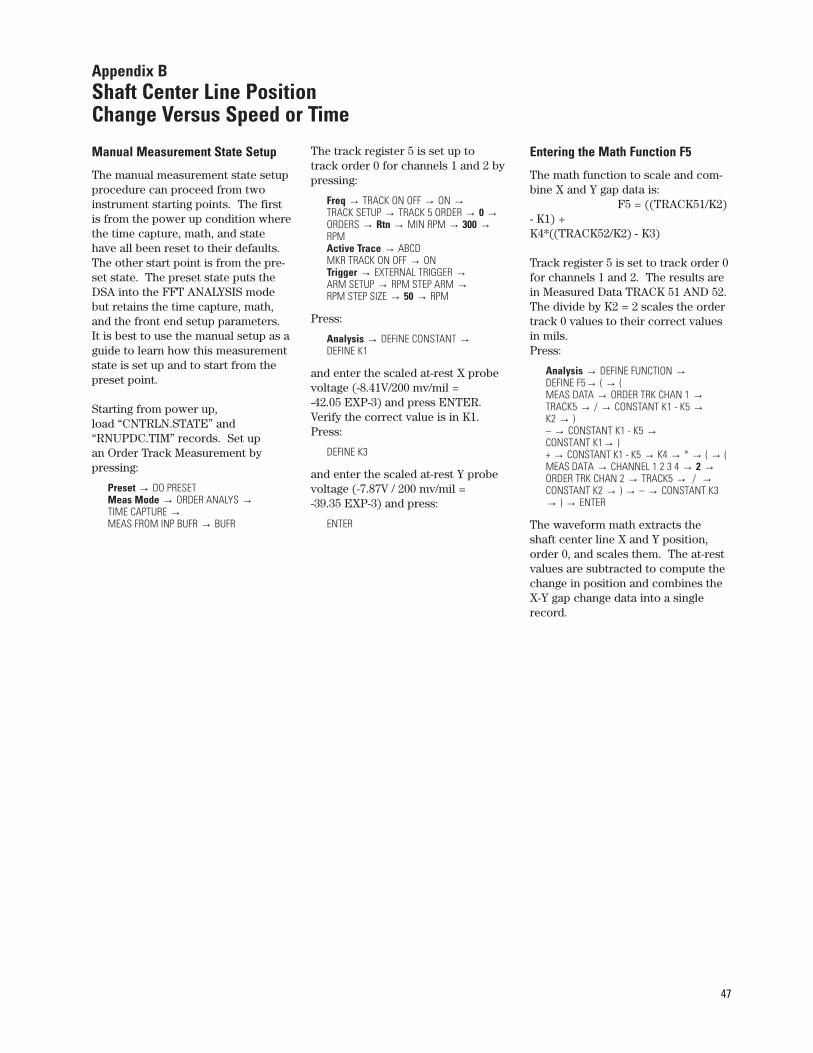
47

Manual Measurement State Setup

The manual measurement state setupprocedure can proceed from twoinstrument starting points. The firstis from the power up condition wherethe time capture, math, and statehave all been reset to their defaults.The other start point is from the pre-set state. The preset state puts theDSA into the FFT ANALYSIS modebut retains the time capture, math,and the front end setup parameters.It is best to use the manual setup as aguide to learn how this measurementstate is set up and to start from thepreset point.

Starting from power up, load “CNTRLN.STATE” and“RNUPDC.TIM” records. Set up an Order Track Measurement bypressing:

Preset → DO PRESET Meas Mode → ORDER ANALYS →TIME CAPTURE →MEAS FROM INP BUFR → BUFR

The track register 5 is set up to track order 0 for channels 1 and 2 bypressing:

Freq → TRACK ON OFF → ON →TRACK SETUP → TRACK 5 ORDER → 0 →ORDERS → Rtn → MIN RPM → 300 →RPMActive Trace → ABCD MKR TRACK ON OFF → ONTrigger → EXTERNAL TRIGGER →ARM SETUP → RPM STEP ARM →RPM STEP SIZE → 50 → RPM

Press:

Analysis → DEFINE CONSTANT →DEFINE K1

and enter the scaled at-rest X probevoltage (-8.41V/200 mv/mil = -42.05 EXP-3) and press ENTER.Verify the correct value is in K1.Press:

DEFINE K3

and enter the scaled at-rest Y probevoltage (-7.87V / 200 mv/mil = -39.35 EXP-3) and press:

ENTER

Entering the Math Function F5

The math function to scale and com-bine X and Y gap data is:

F5 = ((TRACK51/K2)- K1) + K4*((TRACK52/K2) - K3)

Track register 5 is set to track order 0for channels 1 and 2. The results arein Measured Data TRACK 51 AND 52.The divide by K2 = 2 scales the ordertrack 0 values to their correct valuesin mils. Press:

Analysis → DEFINE FUNCTION →DEFINE F5→ ( → ( MEAS DATA → ORDER TRK CHAN 1 →TRACK5 → / → CONSTANT K1 - K5 →K2 → ) – → CONSTANT K1 - K5 →CONSTANT K1→ ) + → CONSTANT K1 - K5 → K4 → * → ( → ( MEAS DATA → CHANNEL 1 2 3 4 → 2 →ORDER TRK CHAN 2 → TRACK5 → / →CONSTANT K2 → ) → – → CONSTANT K3→ ) → ENTER

The waveform math extracts theshaft center line X and Y position,order 0, and scales them. The at-restvalues are subtracted to compute thechange in position and combines theX-Y gap change data into a singlerecord.

Appendix BShaft Center Line Position Change Versus Speed or Time

The Display Setup

The unscaled shaft center line position versus RPM is displayed bypressing:

Disp Format → QUAD Active Trace → A Meas Data → MORE CHOICES →ORDER TRACK CHANNEL 1 →TRACK 5 ORDER 0.00 Active Trace → C Meas Data → MORE CHOICES →CHANNEL 1 2 3 4 → 2 →ORDER TRACK CHANNEL 2 →TRACK 5 ORDER 0.00

The B and D traces are set to displaythe change in X and Y positionextracted with math function F5.

Active Trace → B Meas Data → MORE CHOICES →MATH FUNCTION → F5 Active Trace → D → F5

The trace coordinates for the fourtraces are set up by pressing:

Active Trace → A B C D Trace Coord → Y UNITS →AMPLITUDE PK PP RMS → PKRtn → MORE CHOICES → REAL PART →Active Trace → D → IMAGINARY PART

Assuming you have correctly recalledthe file RNUPDC.Tim, Press:

Start

Scaling the traces is done by pressing:

Scale → AUTOSCALE ON OFF → ON

and at the completion of the measurement press:

AUTOSCALE ON OFF → OFF

The result should look much like Fig. 8.1.

To view the X versus Y shaft centerline position change versus RPM,change the trace coordinates toNYQUIST DIAGRAM.Press:

Disp Format → SINGLE Active Trace → B Trace Coord → MORE CHOICES →NYQUIST DIAGRAMScale → TOP REFERENCE → 1.6 →BOTTOM → -0.4 → MILLI EXP-3

The Nyquist Diagram provides an end view of the shaft position changeversus RPM in the sleeve bearing ofthe rotor kit (Fig. 8.2).

To display the X transducer position change, press:

Trace Coord → MORE CHOICES → REAL Scale → TOP REFERENCE → 1.6 →BOTTOM → -0.4 → MILLI EXP-3

The display on the 35670A will looklike Fig. 8.3. The shaft is pulled tothe left about 0.25 mils at low RPMand then moves to the right about 3 mils at 6400 RPM viewed from themotor end. The motor was turning counterclockwise.

To view the Y gap change versusRPM, press:

Trace Coord → MORE CHOICES →IMAGINARY

The shaft stays at the at-rest positionat low RPM and then rises up on theoil film as RPM increases (Fig. 8.4).

Continue from top of the middle column on page 35.

Product specifications and descriptions in this document subject to change without notice.Copyright © 1998, 2000 Agilent Technologies Printed in U.S.A. 8/005966-0519E

Agilent Technologies' Test and MeasurementSupport, Services, and AssistanceAgilent Technologies aims to maximize the value you receive, while minimizing your risk and problems. We strive to ensure that you get thetest and measurement capabilities you paid forand obtain the support you need. Our extensivesupport resources and services can help you choose the right Agilent products for yourapplications and apply them successfully. Everyinstrument and system we sell has a global war-ranty. Support is available for at least five yearsbeyond the production life of the product. Twoconcepts underlie Agilent's overall support policy: "Our Promise" and "Your Advantage."

Our PromiseOur Promise means your Agilent test and measurement equipment will meet its advertisedperformance and functionality. When you arechoosing new equipment, we will help you withproduct information, including realistic perform-ance specifications and practical recommenda-tions from experienced test engineers. When you use Agilent equipment, we can verify that itworks properly, help with product operation, andprovide basic measurement assistance for the useof specified capabilities, at no extra cost uponrequest. Many self-help tools are available.

Your AdvantageYour Advantage means that Agilent offers a widerange of additional expert test and measurementservices, which you can purchase according toyour unique technical and business needs. Solveproblems efficiently and gain a competitive edgeby contracting with us for calibration, extra-costupgrades, out-of-warranty repairs, and on-siteeducation and training, as well as design, systemintegration, project management, and other professional engineering services. ExperiencedAgilent engineers and technicians worldwide canhelp you maximize your productivity, optimize thereturn on investment of your Agilent instrumentsand systems, and obtain dependable measurementaccuracy for the life of those products.

For More Assistance with Your Test & Measurement Needs go towww.agilent.com/find/assist

Or contact the test and measurement experts at Agilent Technologies (During normal business hours)

United States:(tel) 1 800 452 4844

Canada:(tel) 1 877 894 4414(fax) (905) 206 4120

Europe:(tel) (31 20) 547 2323(fax) (31 20) 547 2390

Japan:(tel) (81) 426 56 7832(fax) (81) 426 56 7840

Latin America:(tel) (305) 267 4245(fax) (305) 267 4286

Australia:(tel) 1 800 629 485 (fax) (61 3) 9272 0749

New Zealand:(tel) 0 800 738 378 (fax) 64 4 495 8950

Asia Pacific:(tel) (852) 3197 7777(fax) (852) 2506 9284

rotor dynamics measurement techniques - agilent technologies

Documents