© by DII-UTOVRM (Dipartimento di Ingegneria dell’Impresa - Università degli Università degli Studi di Roma “Tor Vergata”) This Report has been submitted for publication and will be copyrighted if accepted for publication. It has been issued as a Research Report for early dissemination of its contents. No part of its text nor any illustration can be reproduced without

written permission of the Authors.

Dicembre 2012 RR-21.12

Lucio Bianco Massimiliano Caramia

Stefano Giordani Veronica Piccialli

A Game Theory Approach for Regulating

Hazmat Transportation

A Game Theory Approach for Regulating Hazmat

Transportation

Lucio Bianco ∗ Massimiliano Caramia † Stefano Giordani ‡

Veronica Piccialli§

Abstract

In this paper, we study a novel toll setting policy to regulate hazardous material

(hazmat) transportation, where the regulator (e.g., a government authority) aims

at minimizing not only the network total risk (see Marcotte et al., 2009), but also

spreading the risk in an equitable way over a given road transportation network.

The idea is to use a toll setting policy to discourage carriers transporting hazmat

from overloading portions of the network with the consequent increase of the risk

exposure of the population involved. Specifically, we assume that the toll paid by a

carrier on a network link depends on the usage of that link by all carriers. Therefore

the route choices of each carrier depend on the other carriers choices, and the tolls

deter the carriers from using links with high total risk. The resulting model is a

mathematical programming problem with equilibrium constraints (MPEC), where

the inner problem is a Nash game having as players the carriers, each one wishing to

minimize his/her travel cost (including tolls); the outer problem is addressed by the

government authority, whose aim is finding the link tolls that induce the carriers

to choose route plans that minimize both the network total risk and the maximum

link total risk among the network links (in order to address risk equity). In order

to guarantee the stability of the solution, we study conditions for the existence

and uniqueness of the Nash equilibrium, and propose a local search heuristic for

∗Dipartimento di Ingegneria dell’Impresa, Universita di Roma “Tor Vergata”, Via del Politecnico,

1 - 00133 Roma, Italy. e-mail: bianco@dii.uniroma2.it†Dipartimento di Ingegneria dell’Impresa, Universita di Roma “Tor Vergata”, Via del Politecnico,

1 - 00133 Roma, Italy. e-mail: caramia@dii.uniroma2.it‡Corresponding author. Dipartimento di Ingegneria dell’Impresa, Universita di Roma “Tor Ver-

gata”, Via del Politecnico, 1 - 00133 Roma, Italy. e-mail: stefano.giordani@uniroma2.it§Dipartimento di Ingegneria Civile e Ingegneria Informatica, Universita di Roma “Tor Vergata”,

Via del Politecnico, 1 - 00133 Roma, Italy. e-mail: piccialli@disp.uniroma2.it

1

the MPEC problem based on these conditions. Computational results are carried

out on a real network, comparing the performance of our toll setting policy with

the toll setting approach proposed in Marcotte et al. (2009). The results show the

effectiveness of our approach.

Keywords: Hazardous materials transportation, Toll setting, Bilevel optimization,

Nash game, Heuristic approach.

1 Introduction

What distinguishes the transportation of dangerous goods or hazardous materials (haz-

mats) from the more general freight transport issues is basically the risk associated with

an accidental release of hazmats during their transportation.

Even if statistic data on hazmat transportation (see, e.g., Kara and Verter, 2004)

reveal that the number of accidents is very small compared to the number of hazmat

shipments, both at world level and at national level, this chance imposes a particu-

lar attention to the safety management in order to reduce the occurrence and/or the

consequence magnitude of dangerous events whose impact may be very large in terms

of fatalities, injuries, large-scale evacuations, and severe environmental damage. More

in general, the potential dangers on both the population and the environment make

people very sensitive to this kind of transport. For this reason, hazmat transportation

has stimulated a relevant research investigation.

Hazmat route planning is one of the main issues in hazmat transportation and

deals with selecting where to route hazmat shipment orders among the alternative

paths (routes) between origin-destination pairs on a given road network. The choice

of a path depends on the different objectives that the distinct actors involved in the

decision process want to pursue.

Of course carriers are one of the main actors. From their perspective, shipment

contracts can be considered individually and a route decision between a given origin-

destination pair needs to be made for each shipment with the objective of minimizing

the transportation costs. Thus, for each shipment, this problem focuses on a single-

commodity and a single origin-destination route plan, i.e., a “local route planning

problem” (for a review on this subject see, e.g., the survey of Erkut et al., 2007).

Indeed, hazmat local route planning suffers from some limitations. Since the plans

of the carriers are typically made without taking into account the general context, it

2

may happen that certain links of the transportation network tend to be overloaded with

hazmat traffic. This may result in a considerable increase of the accident probability

on such road links, leading to inequity on the spatial distribution of the risk over the

region where the road transportation network is embedded.

A chance to overcome this difficulty is to consider a government authority charged

with the management of all hazmat shipments within and through its jurisdiction area.

Indeed, although the transportation industry is deregulated in many countries, haz-

mat transportation usually remains part of the governments’ mandate mainly due to

the associated societal and environmental risks. Hence, it is common to assume that

there is a government authority that wants to regulate the hazmat transportation on

the network under its jurisdiction. This authority, in contrast with the single carrier,

has to consider a transportation problem that involves multi-commodities and multiple

origin-destination route decisions, i.e., a “global route planning problem”.

The main concern for a government authority is controlling the risk induced by

hazmat transportation over the population and the environment. Besides the mini-

mization of the total risk, a government authority should also promote equity in the

spatial distribution of risk. This becomes crucial when certain populated zones are ex-

posed to intolerable levels of risk as a result of the carriers’ route decisions. Therefore,

in hazmat global route planning, the main problem (from the authority’s point of view)

is that of finding minimum risk routes, while limiting and equitably spreading the risk

in any area in which the transportation network is embedded.

Since, typically, the government authority does not have the right to impose specific

routes to hazmat carriers, it can only mitigate hazmat transportation risk by means

of policies regulating the use of road segments for hazmat shipments. The scenarios

are essentially two. In the first one, the authority has the right either to close certain

road segments to hazmat vehicles or to limit the amount of hazmat traffic flow on

those network links. In the second scenario, the authority uses link tolls to deter

the carriers from using certain road segments and consequently induces them to route

their shipments on less populated (or risky) links of the network. In the context of

global route planning the first policy falls into the field of “hazmat transportation

network design” (e.g., see the seminal paper of Kara and Verter, 2004), and the second

one belongs to “toll setting policies” (see, e.g., Marcotte et al., 2009). For both cases,

typically the problems addressed by the government authority can be modeled as bilevel

optimization problems. For a survey on bilevel programming, see, e.g., Colson et al.

3

(2005, 2007) and Dempe (2003, 2005).

In particular, in the bilevel problem for toll setting studied by Marcotte et al. (2009),

the outer problem is addressed by the government authority, or regulator (i.e., the leader

in the bilevel problem), that sets tolls on network links that minimize a combination

of total population exposure (i.e., the risk) and total carriers’ travel cost; this is done

taking into account that in the inner problem the carriers (i.e., the followers), each one

independently from each other, select routes minimizing the travel cost (including the

additional cost due to the tolls), given the link tolls set by the government authority.

In this paper, we propose a new toll setting model that extends the one proposed by

Marcotte et al. (2009). A limit of the latter model is that it does not keep into account

risk equity. Indeed, it considers unsplittable hazmat shipments: that is, all the trucks

used by a carrier are assumed to follow the same route selected by that carrier, with the

consequence that it is not possible to distribute and balance (on the whole network)

the risk generated by a carrier transporting a large amount of hazmat. Similarly, it

may happen that a certain link is used by many carriers, resulting in a very high risk

on that link even if the total risk on the network is relatively low.

The aim of the proposed model is to overcome this drawback, assuming a different

toll setting policy where the toll paid by a carrier on a link depends also on the total

risk induced on that link by all the carriers’ route choices. This implies that, differently

from the model of Marcotte et al. (2009), in our model the route choices of each carrier

depend on the other carriers’ choices, and the link tolls are chosen by the government

authority also to deter the carriers from using links with high total risk. The resulting

model is a mathematical programming problem with equilibrium constraints (MPEC)

(see, e.g., Luo et al., 1996, for MPEC), where the inner problem is a Nash game having

as players the carriers, each one choosing a hazmat transportation route plan that

minimizes his/her travel cost (including tolls); the outer problem is addressed by the

government authority, that aims at finding the link tolls that induce the carriers to

choose route plans that minimize both the network total risk and the maximum link

total risk among the network links (in order to address risk equity).

To guarantee the stability of the solution we find conditions for the existence and

uniqueness of the Nash equilibrium, that are valid if all the carriers transport the

same hazmat type. These conditions allow us to reformulate the Nash game as a

strictly convex optimization problem, reducing therefore our MPEC problem to a bilevel

optimization problem. Moreover, we provide toll optimality conditions that allow us to

4

identify the optimal toll setting (with respect to carriers’ cost minimization) inducing a

given a Nash (unique) equilibrium. To solve real case studies, we propose a local search

heuristic for the MPEC problem based on these conditions. Computational results are

carried out on a real network, comparing the performance of our toll setting policy with

the one proposed in Marcotte et al. (2009).

The remainder of the paper is organized as follows. Section 2 contains an overview

of the relevant literature in hazmat global route planning. Section 3 presents the math-

ematical formulation of the considered hazmat toll setting problem. In Section 4, we

show how to solve the Nash game, by identifying existence and uniqueness conditions of

the Nash equilibrium. In Section 5, we study the special case with a single hazmat type

where the above conditions are valid, and provide additional toll optimality conditions

which are exploited in the proposed heuristic approach described in Section 6. Section

7 presents our computational experiments, and Section 8 concludes the paper.

2 Literature overview

Besides minimizing network total risk, one of the main issues addressed in hazmat

global route planning is risk equity, and, hence, finding minimum risk routes, assuring,

at the same time, an equitable distribution of the risk on the interested area where the

given network is embedded. The contributions in this field include the early works of

Zografos and Davis (1989), Gopalan et al. (1990), Lindner-Dutton et al. (1991), and

Marianov and ReVelle (1998). The works of Akgun et al. (2000), Dell’Olmo et al.

(2005), and Carotenuto et al. (2007) on the problem of finding a number of spatially

dissimilar paths between an origin and a destination can also be considered in this

area, along with more recent works proposing multi-objective approaches for selecting

dissimilar paths (see, e.g., Caramia and Giordani, 2009, and Caramia et al., 2010).

The works above reviewed assume that the government authority has the right to

impose routes on individual carriers. However, this is not the case in general. Indeed,

for example, many governments only have the authority to close certain road segments

to hazmat vehicles or to limit the amount of hazmat traffic flow on those links. These

kinds of policies are usually categorized as Hazmat Transportation Network Design

(HTND) policies, and equity concerns can be incorporated into the design objectives.

Kara and Verter (2004) were the first to study the HTND proposing a bilevel integer

programming model by considering the roles of the carriers and of a government author-

5

ity, where the latter imposes restrictions on the network and the carriers then choose the

routes. Since the followers’ problem is linear, the bilevel integer programming problem

is reformulated as a single-level Mixed Integer Programming (MIP) problem by replac-

ing the followers’ problem by its Karush-Kuhn-Tucker (KKT) optimality conditions

and by linearizing the complementary slackness constraints. However, the single-level

reformulation may fail to find an optimal stable solution for the bilevel model. Indeed,

in general, there are multiple minimum-cost route solutions for the followers over the

designed network established by the leader, which may induce different total risk values

over the network, and, hence, the lack of stability of the solution of the bilevel model

provided by the single-level reformulation.

Erkut and Alp (2007) consider the same model of Kara and Verter (2004), restricting

the network to a tree, so that there is a single path between each couple of origin-

destination pair; clearly, with this restriction, the carriers have no alternative paths on

the tree, hence the carriers have no freedom in route selection, with the result that the

structure of the proposed model has a single level.

Erkut and Gzara (2008) generalize the model of Kara and Verter (2004) by con-

sidering the undirected network case and the design of the same network for all the

shipments. They consider the possible lack of stability of the solution of the bilevel

model obtained by solving the single-level reformulation, and propose a heuristic so-

lution method that always finds a stable solution. Moreover, they extend the bilevel

model to account for the cost/risk trade-off by including cost in the objective function

of the leader problem.

Verter and Kara (2008) provide a path-based formulation for the HTND problem

studied by Kara and Verter (2004), where the open links chosen by the regulator in

the given network determine the set of paths that are available to the carriers. This

facilitates the incorporation of carriers’ cost concerns in regulator’s risk reduction de-

cision, and allows to formulate the problem with a single-level integer programming

formulation assuring that the cheapest path among the available ones is used by each

carrier.

Bianco et al. (2009) present a bilevel formulation focused on risk equity. Both levels

correspond to government agencies: the meta-local authority that aims to minimize the

maximum link risk in the whole network, and the regional area authority that aims to

minimize the total risk over the network.

Dadkar et al. (2010) and Reilly et al. (2012) focus on a new HTND problem that

6

takes into account security issues by modeling the possible role of a terrorist.

HTND policies can effectively restrict hazmat shipments in order to induce carri-

ers to route shipments on low-risk paths. However, such a restriction could be too

much since it does not consider the carriers’ priorities, possibly wasting the usability

of certain road segments. Moreover, only restricting certain road segments could not

rationally direct hazmat transportation along less-populated links. An alternative pol-

icy to HTND is proposed by Marcotte et al. (2009) and is based on toll setting. This

Hazmat Transportation Toll Setting (HTTS) policy may discourage (but not prevent)

hazmat carriers from using certain road segments. The authors show that HTTS pol-

icy is a more flexible regulation tool for hazmat transportation than HTND policy.

By imposing tolls on certain road segments, the hazmat shipments are expected to be

directed on less-populated roads according to the carriers’ own selection (due to eco-

nomic considerations) rather than by governors’ restriction. The authors show that the

HTTS model dominates the HTND model since the solution set of the former strictly

contains the solution set of the latter; therefore, the former model may result in a more

attractive policy to regulators since provides more flexible solutions, and at the same

time more acceptable to carriers that maintain the freedom of using any link of the

network.

Marcotte et al. (2009) propose a bilevel model that minimizes the network total

risk and the carriers’ total travel cost, including both transportation costs and toll

fees on the links. They reduce the bilevel problem to a single-level MIP problem by

replacing the followers’ problem with its optimality conditions and by linearizing the

complementary slackness constraints; they also provide an alternative single-level MIP

reformulation where complementary slackness conditions are replaced with the equality

between the primal and dual objective functions of the followers’ problem. Moreover,

they show that the authority can easily find a toll setting inducing a minimum risk

solution by inverse optimization, that is, determining the link tolls that induce the

carriers to choose the minimum risk route plan; hence, in this case, the problem is

not a bilevel problem anymore, but reduces to a single-level problem. However, if the

authority wants to keep into account also carriers’ cost, the problem is a true bilevel

optimization problem.

More recently, Wang et al. (2011) propose a model assuming that both hazmat

traffic and regular traffic affect population safety, since congestion increases delay and

then accident probabilities. The idea is to control both regular and hazmat traffic via

7

toll setting. The authors make the following assumptions: 1) congestion induced by the

traffic flow of hazmat trucks can be ignored; 2) to simplify the model, the users have

perfect information of the current status; 3) all the model parameters are deterministic;

4) a single type of hazmat is considered; 5) travel delay is a linear function of traffic

congestion; 6) risk is linearly affected by travel delay. The authors provide a bilevel

formulation and an equivalent two-stage problem formulation, where the first-stage

problem is a non-convex quadratic programming problem and the latter is a linear

programming problem.

3 Modeling the HTTS problem

Let G = (N,A) be a direct (road transportation) network, with N being the set of

n nodes (intersections in the road network), and A being the set of m directed links

or arcs (road segments) between pairs of nodes. Let A+(i) and A−(i) be the subset

of outgoing links and the subset of ingoing links of node i ∈ N , respectively, that is,

A+(i) = {(i, j) ∈ A : j ∈ N} and A−(i) = {(j, i) ∈ A : j ∈ N}.

Given a set H of hazmat type, we consider a set K of p carriers, with carrier k ∈ K

having to satisfy a single shipment order (commodity) of amount bk of hazmat of type

h(k) ∈ H, from origin node sk to destination node tk. Accordingly, let eki be equal

to 1,−1 or 0 depending on whether node i ∈ N is the origin node (i.e., i ≡ sk), the

destination node (i.e., i ≡ tk), or a transshipment node (i.e., i 6= sk, tk) for carrier k.

For the sake of simplicity, we assume that carrier k uses a fleet of homogeneous

trucks (vehicles) each one of capacity qk and traveling at full load (hence, we may

assume that the shipment order ratio bk

qkrepresents the number of hazmat trucks used

by carrier k for the hazmat shipment).

Let cij ≥ 0 be the truck transportation cost (or length) of link (i, j) ∈ A, and let ρhij

be the risk (e.g., the number of exposed persons) induced by a truck carrying hazmat

of type h through link (i, j) ∈ A; without loss of generality, we assume that ρhij > 0, for

each (i, j) ∈ A.

According to HTTS policy, we assume that there is a government authority that

wishes to mitigate the risk induced by hazmat shipments by regulating hazmat trans-

portation via toll setting. Specifically, in the HTTS problem, the authority wishes to

determine the amount of toll fee to be set on all the links of the network, in order to

deter the carriers from using certain road segments and encourage them to use, e.g., the

8

less populated ones. The aim is that of limiting as much as possible the risk over the

network. On the other side, the carriers make their routing decisions, e.g., minimizing

their total transportation and toll cost.

3.1 The model of Marcotte et al. (2009)

Marcotte et al. (2009) model the HTTS problem in terms of the following NP-hard

bilevel problem:

minτhij

∑

k∈K

∑

(i,j)∈A

(ρh(k)ij + α(cij + τ

h(k)ij ))

bk

qkxkij

s.t. τhij ≥ 0, ∀ (i, j) ∈ A, ∀h ∈ H

where xkij solves:

minxkij

∑

k∈K

∑

(i,j)∈A

(cij + τh(k)ij + βρ

h(k)ij )

bk

qkxkij

s.t.∑

(i,j)∈A+(i)

xkij −∑

(j,i)∈A−(i)

xkji = eki , ∀ i ∈ N, ∀ k ∈ K

xkij ∈ {0, 1}, ∀ (i, j) ∈ A, ∀ k ∈ K,

(1)

where τhij and xkij are the variables controlled by the leader and the followers, respec-

tively. In particular,

• τhij are non-negative variables representing the tolls imposed by the authority on

link (i, j) ∈ A, for each truck transporting hazmat of type h ∈ H;

• xkij are binary variables modeling the decisions of the carriers, and are equal to 1

if link (i, j) ∈ A is used by carrier k for the shipment, 0 otherwise.

In this model the leader (i.e., the authority) sets the tolls on the network links

in such a way to minimize a weighted combination (through weight parameter α) of

the network total risk and carriers’ total cost. This is done by keeping into account

that, for a given set of values of the link tolls, the followers (i.e., the carriers) choose,

independently from each other, the minimum cost routes (assuming, e.g., β = 0) from

their origin node to their destination nodes.

3.2 The proposed model

Differently from the model of Marcotte et al. (2009), we assume that:

9

1. the authority aims at minimizing not only the network total risk (and the carriers’

total cost), but also achieve the risk equity.

2. the decision variables controlled by the carriers are continuous;

Therefore, in our model, let xkij, with 0 ≤ xkij ≤ 1, be the decision variables con-

trolled by carrier k, representing the fraction of its shipment routed along link (i, j),

for each (i, j) ∈ A. Of course, each carrier k, with k ∈ K, makes routing choice mini-

mizing his own transportation cost, that, without considering additional cost, is equal

to∑

(i,j)∈A cijbk

qkxkij .

The authority, on the basis of the above assumption 1, wishes to minimize the

network total risk, that is,∑

k∈K

∑

(i,j)∈A

ρh(k)ij

bk

qkxkij,

and pursue the risk equity by minimizing the maximum link total risk among the links

of the network, that is,

max(i,j)∈A

{∑

k∈K

ρh(k)ij

bk

qkxkij}.

While Marcotte et al. (2009) (see model formulation (1)) assume that the amount

of toll fee that carrier k should pay for using a link is proportional to the number bk

qk

of its hazmat vehicles routed on that link, and, hence, proportional to the amount of

the risk induced by its hazmat shipment on the link, in our model we assume that the

amount of the toll paid by a carrier for using a link is a quadratic function of the total

amount of the risk that all the carriers’ shipments induce on that link.

Therefore, the additional travel cost (due to toll fees) faced by each carrier depends

also on the hazmat route plans of the other carriers, since the amount of toll fee that

a carrier has to pay for using a link depends on the total risk on that link. The aim

of our assumption is to induce the carriers to transport hazmat along routes where the

total risk is lower, and at the same time to limit the amount of total risk on each single

link.

More in detail, for each link (i, j) ∈ A, let Th(k)ij be the toll fee that carrier k has

to pay for each unit of risk induced by its shipment on link (i, j). As the idea is to

discourage carrier k from using a link with high total risk, with the latter being induced

by carrier k and all the other carriers that use that link, tax Th(k)ij per unit of risk is

assumed to be the sum of the following two terms, that is

10

Th(k)ij = t

h(k)ij + d

h(k)ij

∑

ℓ∈K

ρh(ℓ)ij

bℓ

qℓxℓij , (2)

where th(k)ij and d

h(k)ij are toll parameters used to weight the risk contribution of carrier k

with respect to the risk caused by the whole set of carriers. In particular, toll parameter

th(k)ij is associated to the risk induced by carrier k on link (i, j) (similarly to model (1)

of Marcotte et al., 2009), and toll parameter dh(k)ij is related to the total risk induced

by all the carriers on the same link.

Therefore the toll fee paid by carrier k for routing a fraction xkij of its shipment on

link (i, j) ∈ A is equal to

th(k)ij ρ

h(k)ij

bk

qkxkij + d

h(k)ij

∑

ℓ∈K

ρh(ℓ)ij

bℓ

qℓxℓij

ρh(k)ij

bk

qkxkij. (3)

The linear component (weighted by toll parameter th(k)ij ) is used to regulate the total

risk on the network similarly to the HTTS model (1) of Marcotte et al. (2009), while

the quadratic component (weighted by toll parameter dh(k)ij ) is used to control the

maximum link total risk, possibly forcing carrier k to split his order amount bk along

different routes. Thus, given an assignment of values to toll parameters thij and dhij by

the government authority, the objective function of the subproblem of each carrier k

becomes

θk(x; t,d) =∑

(i,j)∈A

cijbk

qkxkij +

∑

(i,j)∈A

th(k)ij ρ

h(k)ij

bk

qkxkij+

∑

(i,j)∈A

dh(k)ij

∑

ℓ∈K

ρh(ℓ)ij

bℓ

qℓxℓij

ρh(k)ij

bk

qkxkij,

(4)

where x denotes the vector containing all the carriers’ variables xkij, and t,d denote

the vectors of toll parameters thij , dhij , respectively. Therefore, the carriers’ problem

constitutes a Nash Equilibrium Problem (NEP), where each carrier k is a player and

his subproblem is

11

minxkij

θk(x; t,d)

s.t.∑

(i,j)∈A+(i)

xkij −∑

(j,i)∈A−(i)

xkji = eki , ∀ i ∈ N

xkij ≥ 0, ∀ (i, j) ∈ A.

(5)

Due to the compactness of the feasible set of each player’s subproblem, the Nash

game admits a solution for every value of toll parameters thij and dhij . Unfortunately, in

general, uniqueness of the equilibrium is not guaranteed, leading to a possible lack of

stability of the solution of our HTTS model (6) formulated below.

Taking into account the roles of the authority and of the carriers, the whole model is

a bilevel problem, where the leader (i.e, the authority) sets tolls on the network links by

choosing the values of toll parameters thij and dhij in order to minimize a combination of

risk magnitude and carriers travel cost. The followers (i.e., the carriers) are the players

of the Nash game, where each player k, with k ∈ K, aims at solving subproblem

(5) on the toll network, and hence selects the route plan for his/her shipment by

controlling variables xkij . In particular the leader wants to minimize the risk magnitude

by minimizing the total risk on the network, and the maximum link total risk among

the links of the network; in addition the regulator may want to minimize the carriers’

total cost. In this situation, we get the following MPEC problem:

mint,d

z = w1

∑

k∈K

∑

(i,j)∈A

ρh(k)ij

bk

qkxkij + w2 · Φ+ w3

∑

k∈K

θk(x; t,d)

s.t.∑

k∈K

ρh(k)ij

bk

qkxkij ≤ Φ, ∀ (i, j) ∈ A

thij ≥ 0, dhij ≥ 0, ∀ (i, j) ∈ A, ∀h ∈ H

where x is a Nash Equilibrium (NE) of

minxkij

θk(x; t,d)

s.t.∑

(i,j)∈A+(i)

xkij −∑

(j,i)∈A−(i)

xkji = eki , ∀ i ∈ N

xkij ≥ 0, ∀ (i, j) ∈ A

for all k ∈ K,

(6)

12

s3 s1 a

b

s2 c d t1

t3 t2

(1, 1) (2, 1)

(1.5, 1)(1, 1.75) (3, 2.5)(3, 1)

(1, 1)

(1.5, 1)

(1, 1) (1, 1.75)

(1, 1)

(1, 0.5)

(1, 1)

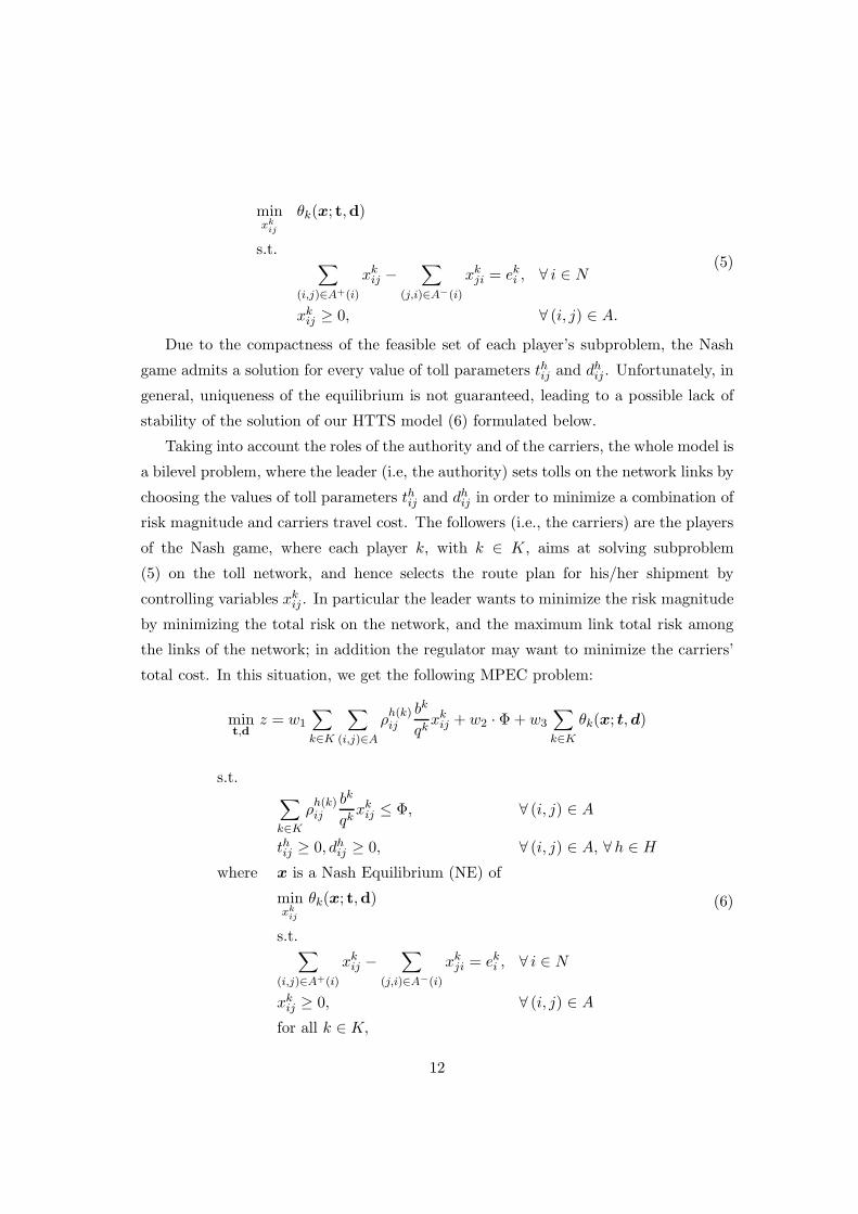
Figure 1: An example: for each link (i, j), the label represents (cij , ρ1ij).

where Φ is a continuous variable representing the maximum link total risk, and w1, w2,

and w3 are weight factors that allow one to control the preference of the leader with

respect to the different aspects he wants to control.

3.3 An example

In order to show the advantages of our HTTS model (6) with respect to the model (1)

of Marcotte et al. (2009) (and also w.r.t. HTND policy), let us consider an example

on the small network shown in Figure 1, with three carriers (i.e., K = {1, 2, 3}) all

shipping the same type of hazmat (i.e., h(k) = 1, for each k = 1, 2, 3). Let (sk, tk)

be the origin-destination pair of the shipment of carrier k. Let us assume that carrier

1 needs two trucks for its shipment and each one of the others only one truck (i.e.b1

q1= 2, b2

q2= b3

q3= 1). For each link (i, j) ∈ A, the values in brackets shown in the

figure represent the cost cij and the risk ρ1ij on the link per unit of truck, respectively.

Note that for both carriers 2 and 3 there is a single path connecting the origin to

the destination of the shipment: that is, path (s2 → c → d → t2) and path (s3 →

s1 → c → t3) for carriers 2 and 3, respectively; these two paths pass through link (c, d)

and (s1, c), respectively, where there is the highest population exposure (risk). On the

contrary, there are multiple paths available to carrier 1 for traveling from its origin

node s1 to its destination node t1.

In particular, for carrier 1 the most attractive path is of course the minimum cost

13

path, that is path (s1 → c → d → t1). If carrier 1 follows this path (i.e., in the

unregulated scenario) the network total risk will be 15.5, and the maximum link total

risk 5.25 (on links (s1, c) and (c, d)). The total transportation cost will be 12, which of

course is the minimum value.

On the other hand, if the authority had the right to impose routes to carriers (i.e., in

the over-regulated scenario), the authority would choose a minimum risk path for carrier

1, that is, equivalently either path (s1 → a → d → t1) or path (s1 → b → d → t1),

getting the (minimum) network total risk of value 12.5. In particular to achieve also

risk equity, the authority would assign one of these two paths to truck 1 and the other

to truck 2 of carrier 1 in order to minimize also the maximum link total risk, which

would be equal to the minimum value of 1.75 (on links (s1, c) and (c, d)). The total

transportation cost would be 16.

With a HTND policy (e.g., according to the model of Kara and Verter, 2004), the

authority would close link (d, t1) in order to prevent carrier 1 from using the larger risky

path (s1 → c → d → t1) (note that links (s1, c) and (c, d) cannot be closed otherwise

the other two carriers would not have any available path for their shipments). With this

link closure, carrier 1 would be forced to choose path (s1 → a → t1). Therefore with

the HTND policy the total risk on the network would be equal to 14.5. The maximum

link total risk would be 5 (on link (a, t1)), and the total transportation cost would be

16.

With the HTTS model (1) of Marcotte et al. (2009), the authority may set the tolls

τ1ij (e.g., sufficiently large on links (s1, c) and/or (c, d)) so that carrier 1 chooses the

minimum (transportation + toll) cost path (s1 → b → d → t1) getting a network total

risk of minimum possible value, i.e., 12.5. The maximum link total risk would be equal

to 2 (on links (s1, b) and (b, d)), and the total transportation cost equal to 15 + ǫ, with

ǫ being a small value greater than 0 (including a toll of value 1 + ǫ paid by carrier 3

assuming to have set this value for the toll τs1,c on link (s1, c)).

The example shows that HTTS policy would induce a lower risk than HTND policy,

while the opposite behavior cannot be obtained. This difference is due to the flexibility

of HTTS policy that allows to differentiate the behavior among carriers: indeed, it may

happen that a carrier chooses a certain link despite the toll, while if a link is closed

to the transportation of a given hazmat type, it becomes forbidden for all carriers

transporting that type of hazmat.

With our HTTS model (6), we can obtain the same result of model (1) in term of

14

network total risk, but a lower maximum link total risk. Indeed, model (1) provides a

network total risk equal to the minimum value 12.5, but it is reached without taking

into account the risk equity, and in particular all the amount of the shipment order of

a carrier is shipped along the same route. By using our model (6), since the carriers’

variables xkij are assumed to be continuous, it is possible to set the tolls (e.g., t1s1,c

=

(3 + ǫ)/ρ1s1,c

, t1a,t1

> 1/ρ1a,t1

, and d1b,d = 1) in order to induce carrier 1 to split its

hazmat flow along the two minimum risk paths (s1 → a → t1) and (s1 → b → d → t1),

getting again the (minimum) network total risk of value 12.5, but a lower maximum link

total risk of value 1.75 (on links (s1, c) and (c, d)), which is in particular the minimum

possible value. Finally, the total transportation cost is 21 + ǫ (including a toll of value

3 + ǫ paid by carrier 3 on link (s1, c)). In conclusion, the example shows that model

(6) is able to achieve the same network total risk and a better distribution of the risk

with respect to model (1) of Marcotte et al. (2009). Therefore, our model can provide

solutions dominating those of the latter model (considering the network total risk and

the maximum link total risk as performance measures). Note that the opposite cannot

occur because the feasible set of model (6) strictly contains the feasible set of model

(1): indeed, the latter can be obtained by fixing to zero the value of parameters dhij of

our model.

4 Properties of the NEP

To simplify the notation, in this section let us denote with {1, 2, . . . ,m} the set A of the

network links, and let a ∈ A be a generic link. Moreover, let us denote with xk ∈ ℜm

the vector of variables controlled by carrier k, with k = 1, . . . , p.

We focus on the properties of the Nash game (5) among the carriers. The objective

function θk(x; t,d) of player (carrier) k is a continuously differentiable quadratic func-

tion of x, that is convex with respect to the variables of the player since the hessian

with respect to xk is equal to the diagonal matrix

∇2xkθk(x; t,d) =

2dh(k)1 (ρ

h(k)1

bk

qk)2 0 . . . 0

0 2dh(k)2 (ρ

h(k)2

bk

qk)2 . . . 0

......

. . ....

0 0 . . . 2dh(k)m (ρ

h(k)1

bk

qk)2

15

that is positive semidefinite for any dh(k)a ≥ 0 of link a ∈ A. Furthermore, denoted with

Dk =

xk ∈ ℜm :∑

a∈A+(i)

xka −∑

a∈A−(i)

xka = eki , ∀ i ∈ N ; xka ≥ 0, ∀ a ∈ A

the feasible set of each player k, we have that Dk is compact and convex.

It is well known (see, e.g., Proposition 1.4.2 in Facchinei and Pang, 2003) that

given the convexity of θk(x; t,d) and the convexity and compactness of Dk, for each

k = 1, . . . , p, Nash game (5) is equivalent to the variational inequality V I(D,F ), where

D =p∏

k=1

Dk, F (x) =

∇x1θ1(x; t,d)

∇x2θ2(x; t,d)...

∇xpθp(x; t,d)

. (7)

The gradient of the objective function θk(x; t,d) with respect to variables xka of

carrier k, with a ∈ A, is a vector of m components whose generic element is given by

∂θk(x; t,d)

∂xka= ca

bk

qk+ th(k)a ρh(k)a

bk

qk+ dh(k)a ρh(k)a

bk

qk

(

ρh(k)a

bk

qkxka +

p∑

ℓ=1

ρh(ℓ)a

bℓ

qℓxℓa

)

, (8)

so that

∇xkθk(x) =

c1bk

qk+ t

h(k)1 ρ

h(k)1

bk

qk+ d

h(k)1 ρ

h(k)1

bk

qk

(

ρh(k)1

bk

qkxk1 +

p∑

ℓ=1

ρh(ℓ)1

bℓ

qℓxℓ1

)

c2bk

qk+ t

h(k)2 ρ

h(k)2

bk

qk+ d

h(k)2 ρ

h(k)2

bk

qk

(

ρh(k)2

bk

qkxk2 +

p∑

ℓ=1

ρh(ℓ)2

bℓ

qℓxℓ2

)

...

cmbk

qk+ th(k)m ρh(k)m

bk

qk+ dh(k)m ρh(k)m

bk

qk

(

ρh(k)m

bk

qkxkm +

p∑

ℓ=1

ρh(ℓ)m

bℓ

qℓxℓm

)

.

(9)

Since the sets Dk are compact, and F (x) is a vector of continuous functions, a

solution of the V I(D,F ) (and, hence, a Nash equilibrium of NEP (5)) always exists. A

sufficient condition for having uniqueness of the solution is F (x) being strictly mono-

tone on D, that is

(F (x)− F (y))T(x− y) > 0, ∀x, y ∈ D ,x 6= y.

Since our F (x) is a vector of affine functions, the Jacobian of F (x) (denoted with

matrix JF (x)) is a constant matrix, and a sufficient condition for the strong (and,

16

hence, strict) monotonicity of F (x) is JF (x) being positive definite. In order to eval-

uate JF (x), we note that

∂2θk(x; t,d)

∂2xka= 2dh(k)a

(

ρh(k)a

bk

qk

)2

;∂2θk(x; t,d)

∂xℓa∂xka

= dh(k)a ρh(k)a

bk

qkρh(ℓ)a

bℓ

qℓ;

∂2θk(x; t,d)

∂xka′∂xka

= 0 ;∂2θk(x; t,d)

∂xℓa′∂xka

= 0.

Therefore, JF (x) is the (pm× pm) matrix

JF (x) =

H11 H12 . . . H1p

H21 H22 . . . H2p...

.... . .

...

Hp1 Hp2 . . . Hpp

where

Hkℓ =bk

qkbℓ

qℓ

dh(k)1 ρ

h(h)1 ρ

h(ℓ)1 0 . . . 0

0 dh(k)2 ρ

h(k)2 ρ

h(ℓ)2 . . . 0

0 0 . . . dh(k)m ρ

h(k)m ρ

h(ℓ)m

for k 6= ℓ, and

Hkk =

(

bk

qk

)2

2dh(k)1

(

ρh(k)1

)20 . . . 0

0 2dh(k)2

(

ρh(k)2

)2. . . 0

0 0 . . . 2dh(k)m

(

ρh(k)m

)2

.

This matrix in general cannot be expected to be positive definite. Note that the matrix

JF (x) is not symmetric. Furthermore, it is evident from the structure of JF (x) that

as soon as a single dh(k)a , with a ∈ {1, 2, . . . ,m}, is equal to zero, then the matrix is not

positive definite (an element on the diagonal is zero).

However, if we focus on the particular case where all the carriers transport the same

hazardous material h (which is equivalent to remove the superscript h(k)), then the

following proposition can be stated:

Proposition 4.1 If all the carriers transport the same hazardous material, i.e. h(k) =

h for all k = 1, . . . , p, then for any value of the toll parameters ta and da > 0, for

a = 1, . . . ,m:

17

(i) there exists a unique equilibrium of NEP (5).

(ii) NEP (5) is equivalent to the following strictly convex optimization problem:

min κTx+1

2xTJF (x)x

s.t.

∑

a∈A+(i)

xka −∑

a∈A−(i)

xka = eki , ∀ i ∈ N, ∀ k = {1, . . . , p}

xka ≥ 0, ∀a ∈ A, ∀ k = {1, . . . , p},

(10)

where

κ =

(c1 + t1ρ1)b1

q1...

(cm + tmρm)b1

q1...

(c1 + t1ρ1)bp

qp...

(cm + tmρm)bp

qp

.

Proof.

(i) The existence of an equilibrium is implied by the compactness of feasible set Dk

of each player k. As for the uniqueness, under the assumption h(k) = h for all

k = 1, . . . , p the jacobian matrix JF (x) is symmetric and of the form

JF (x) =

2(

b1

q1

)2H b1b2

q1q2H . . . b1bp

q1qpH

b2b1

q2q1H 2

(

b2

q2

)2H . . . b2bp

q2qpH

......

. . ....

bpb1

qpq1H bpb2

qpq2H . . . 2

(

bp

qp

)2H

where, by denoting with Diag(v) the diagonal matrix having as elements on the

diagonal the elements of vector v,

H = Diag(

(ρa)2da)m

a=1.

18

By setting

r =

b1

q1

...bp

qp

,

this matrix can be equivalently rewritten as

JF (x) = H ⊗(

rrT +Diag(r))

,

where operator ⊗ indicates the Kronecker product of two matrices. Matrix H is a

diagonal matrix having eigenvalues equal to the elements of the diagonal, so that

it is positive definite if we assume that all the diagonal elements of H are positive

(i.e., all the toll parameters da and risk coefficient ρa are positive). As for the

matrix rrT + Diag(r), it is positive definite since it is a rank one update of the

positive definite matrix Diag(r) having as eigenvalues bk

qk> 0, for k = 1, . . . , p.

Therefore, since the Kronecker product of two positive definite matrices is positive

definite, then the matrix JF (x) is positive definite, implying strict monotonicity

of the function F (x). Therefore, we have a unique equilibrium.

(ii) As proved in point (i), under the assumption h(k) = h, for all k = 1, . . . , p, the

jacobian matrix JF (x) is symmetric. It is well known (see, e.g., Theorem 1.3.1 in

Facchinei and Pang, 2003) that given a vector F (x) of continuously differentiable

functions, if its jacobian is symmetric, then there exists a real-valued function

ϕ(x) such that ∇ϕ(x) = F (x), and

ϕ(x) =

∫ 1

0FT (x0 + t(x− x0)) (x− x0) dt.

By the expression of F (x), it follows that

ϕ(x) = κTx+1

2xTJF (x)x,

that is a quadratic function, with hessian equal to JF (x) which is proved at point

(i) to be positive definite. Therefore, function ϕ(x) is strictly convex, so that

problem (10) has a unique solution. Finally, the well known minimum principle

applied to problem (10) is equivalent to solving the V I(D,F ), and the thesis

follows.

19

The above proposition justifies the attention to the special case where all the carriers

transport the same type of hazardous material, situation that occurs in particular in

the experiments on the network of Ravenna, Italy, given in Erkut and Gzara (2008)

and in the experiments reported in Section 7. In the next section we consider in depth

all the implications of Proposition 4.1.

5 The single hazardous material case

From now on, we assume that the hypothesis of proposition 4.1 are verified, i.e., h(k) =

h, for every carrier k = 1, . . . , p.

Point (i) of Proposition 4.1 states that if we restrict toll parameters dij to strictly

positive values, for each (i, j) ∈ A, the equilibrium of Nash game (5) is unique. This

result ensures stability of the solutions of the bilevel problem (6), which is an extremely

rare result in bilevel programming. Indeed, whenever ties among inner-level solutions

(carriers’ route plans) occur, in general the bilevel formulation assumes that carriers

adopt the one that minimizes the leader’s objective. This is true also for the bilevel

model of Marcotte et al. (2009), where however in principle a perturbation of the tolls

may be used in order to break the ties.

A crucial point for the viability of the game theory approach is how to solve the

Nash game (5), possibly by a distributed algorithm requiring a reasonable exchange of

information between the players, since it is not realistic to assume the presence of an

external agent that, on behalf of the carriers, solves the Nash game and returns the

route plans to the carriers.

With this respect, point (ii) of Proposition 4.1 and its proof provide a satisfactory

result. Indeed, they imply that, in the special case of a single type of hazmat, Nash

game (5) is a potential game. Potential game are defined in Monderer and Shapley

(1996) as follows: a game where each player k = 1, . . . , p has to solve the problem

minxk

θk(x)

s.t. xk ∈ Dk,

is an exact potential game if there exist a function P (x) such that

∇xkP (x) = ∇xkθk(x), for every k = 1, . . . , p.

20

Proof of point (ii) of Proposition 4.1 implies that the objective function of problem (10)

is an exact potential for Nash game (5). Whenever a game is potential, any solution of

the problem

min P (x)

s.t. xk ∈ Dk, k = 1, . . . , p

is a Nash equilibrium of NEP (5).

Another important consequence of Nash game (5) being potential is that a best

response algorithm converges to a Nash equilibrium. Therefore, it can be solved by

means of distributed algorithms of the following form:

Step 0. Choose a starting point x(0) = (x1(0), . . . , xp(0)) ∈

∏pk=1Dk, and set i := 0.

Step 1. If x(i) satisfies a suitable termination criterion: STOP.

Step 2. FOR k = 1, . . . , p

Compute a solution xk(i+1) of

minxk

θk(x1(i+1), . . . , x

k−1(i+1), x

k, xk+1(i) , . . . , xp(i))

s.t. xk ∈ Dk

(11)

END

Step 3. Set x(i+1) := (x1(i+1), . . . , xp(i+1)), i := i+ 1, and go to Step 1.

Looking at the expression (4) of the carrier’s objective function θk(x; t,d), it results

that, for a given set of values of toll parameters tij, dij , the only information that the

carriers need to exchange is the link total risk∑p

ℓ=1 ρh(ℓ)ij

bℓ

qℓxℓij on each link (i, j) ∈ A,

with no need to know exactly the route plans of the other carriers. Note that this is

the minimum requirement on information exchange among the carriers.

This algorithm can also be interpreted equivalently as a Gauss Seidel type algo-

rithm for the optimization problem (10), and it is well known that thanks to the strict

convexity of the objective function, it converges to the unique solution.

Given a set of values (t, d) of the toll parameters tij and dij , with tij ≥ 0 and dij > 0,

for each (i, j) ∈ A, the corresponding Nash equilibrium, denoted with x(t, d), is unique.

However, in general different toll parameters’ values can induce the same equilibrium.

An interesting question from the authority point of view, is what is the “best” set of

21

values for the toll parameters with respect to some criterion (e.g., minimizing the total

cost paid by the carriers) inducing the Nash equilibrium x(t, d).

Assume that corresponding to a given set of non-negative toll parameters’ values

tij, dij (with dij > 0), a certain Nash equilibrium x(t, d) has been computed. This

implies that x = x(t, d) is the only point satisfying the following KKT optimality

conditions of problem (10) when tij = tij, dij = dij , for every k = 1, . . . , p:

cijbk

qk+ ρij

bk

qktij +

[

ρijbk

qk

(

ρijbk

qkxkij +

p∑

ℓ=1

ρijbℓ

qℓxℓij

)]

dij − µki + µk

j − λkij = 0, ∀ (i, j) ∈ A

λkijx

kij = 0, ∀ (i, j) ∈ A

∑

(i,j)∈A+(i)

xkij −∑

(j,i)∈A−(i)

xkji = eki , ∀ i ∈ N

xkij ≥ 0, ∀ (i, j) ∈ A

λkij ≥ 0, ∀ (i, j) ∈ A

µki free, ∀ i ∈ N,

(12)

where λkij for (i, j) ∈ A, and µk

i for i ∈ N are the dual variables corresponding to the

constraints of carrier k ∈ K.

Denoting with φij(x) =p∑

ℓ=1

ρijbℓ

qℓxℓij the link total risk on link (i, j) ∈ A correspond-

ing to equilibrium x, and letting γkij(x) = ρijbk

qk

(

ρijbk

qkxkij + φij(x)

)

, conditions (12),

for each carrier k = 1, . . . , p, can be rewritten as the following linear constraints in the

variables tij, dij, µki ,

cijbk

qk+ ρij

bk

qktij + γkij(x)dij − µk

i + µkj ≥ 0, ∀ (i, j) ∈ A\Ak

cijbk

qk+ ρij

bk

qktij + γkij(x)dij − µk

i + µkj = 0, ∀ (i, j) ∈ Ak

µki free, ∀ i ∈ N,

(13)

where Ak = {(i, j) ∈ A : xkij > 0}, and having omitted the flow conservation constraints

on the network nodes and the non-negative constraints on the values of carriers’ vari-

ables xkij because they are obviously satisfied at x, since x ∈∏p

k=1Dk.

Now, let us assume that, given equilibrium x = x(t, d), the government authority

is interested in finding the optimal vectors (t∗,d∗) of toll parameters that induce the

carriers to reach the given equilibrium x, and such that the total cost ζ(x; t,d) paid

22

by the carriers (including toll fees) is minimized, where

ζ(x; t,d) =p∑

k=1

∑

(i,j)∈A

cijbk

qkxkij +

p∑

k=1

∑

(i,j)∈A

tijρijbk

qkxkij

+p∑

k=1

∑

(i,j)∈A

dij

(

p∑

ℓ=1

ρijbℓ

qℓxℓij

)

ρijbk

qkxkij

=p∑

k=1

∑

(i,j)∈A

cijbk

qkxkij +

∑

(i,j)∈A

φij(x)tij +∑

(i,j)∈A

(φij(x))2 dij .

(14)

Note that ζ(x; t,d) is a linear function of tij and dij .

Therefore, finding the optimal toll parameters’ values is equivalent to solving a

suitable Linear Programming (LP) problem, having the optimality conditions (13) for

k = 1, . . . , p as constraints, and minimizing ζ(x; t,d); that is, the LP problem

mintij ,dij ,µ

ki

ζ(x; t,d) =p∑

k=1

∑

(i,j)∈A

cijbk

qkxkij +

∑

(i,j)∈A

φij(x)tij +∑

(i,j)∈A

(φij(x))2 dij

s.t.

cijbk

qk+ ρij

bk

qktij + γkij(x)dij − µk

i + µkj ≥ 0, ∀ (i, j) ∈ A\Ak, k = 1, . . . , p

cijbk

qk+ ρij

bk

qktij + γkij(x)dij − µk

i + µkj = 0, ∀ (i, j) ∈ Ak, k = 1, . . . , p

dij ≥ ǫ, ∀ (i, j) ∈ A

tij , dij ≥ 0, ∀ (i, j) ∈ A

µki free, ∀ i ∈ N, k = 1, . . . , p,

(15)

where ǫ is a small value greater than 0.

We note that this problem is well posed. Indeed, it has a nonempty feasible set

since toll settings tij, dij are feasible and the objective function assumes nonnegative

values and hence is bounded from below.

6 A heuristic resolution approach

Even in the favorable case where all the carriers transport the same type of hazardous

material, it is hard to solve problem (6) (that, in this case, reduces to a bilevel opti-

mization problem), and few exact algorithms are available for this aim, keeping also

23

in mind that reasonable size networks lead to large size instances of the corresponding

bilevel problem.

Therefore, we propose to heuristically solve the problem with a local search algo-

rithm that exploits existence, uniqueness, and efficient computation of the equilibrium

x(t,d) of the Nash game (5) among the carriers (i.e., the followers), corresponding to

a given set of values (t,d) of toll parameters tij , dij (with tij ≥ 0 and dij > 0), for each

link (i, j) ∈ A, chosen by the government authority (i.e., the leader). The idea is to

explore heuristically the leader’s search space using the corresponding Nash equilibrium

in order to evaluate the effectiveness of the leader’s choice.

Note that, given any toll setting (t,d), the corresponding unique equilibrium x(t,d)

can be found by solving problem (10) with any valid optimization algorithm for it,

including the distributed algorithm given in Section 5. Therefore any given toll setting

(t,d) (along with the induced unique equilibrium x(t,d)) represents a feasible solution

of the bilevel problem.

We measure the goodness of a given toll setting (solution) (t,d) with the following

performance indices, representing the network total risk, the maximum link total risk

and the cost paid by the carriers, respectively, given their choices x(t,d):

Rtot(x(t,d)) =∑

(i,j)∈A

∑

k∈K

ρijbk

qkxkij =

∑

(i,j)∈A

φij(x(t,d));

Φ(x(t,d)) = max(i,j)∈A

∑

k∈K

ρijbk

qkxkij

= max(i,j)∈A

{φij(x(t,d))} ;

Ctot(x(t,d)) =∑

k∈K

∑

(i,j)∈A

cijbk

qkxkij +

∑

k∈K

∑

(i,j)∈A

tijρijbk

qkxkij

+∑

k∈K

∑

(i,j)∈A

dij

∑

ℓ∈K

ρijbℓ

qℓxℓij

ρijbk

qkxkij =

∑

k∈K

∑

(i,j)∈A

cijbk

qkxkij +

∑

(i,j)∈A

tij φij(x(t,d)) +∑

(i,j)∈A

dij [φij(x(t,d))]2.

We consider an Old Bachelor Acceptance (OBA) local search approach, that is a

Threshold Acceptance (TA) strategy where the threshold changes dynamically, up and

down, based on the perceived likelihood of being near a local minimum (see, e.g., Hu

et al., 1995). Such classes of local search strategies overcome the typical drawback of

standard TA approaches where the threshold is monotonically decreased during the

search, with the consequence that after a certain number of iterations if the current

solution is not worse than its neighbors the TA algorithm will fail to move to another

24

solution of the neighborhood of the current one. With the OBA strategy the criterion

for accepting a neighbor of the current solution is relaxed by increasing the threshold,

and after a certain number of fails in moving to another solution, the threshold will

become sufficiently large to escape from the current local optimum; therefore in this way

OBA applies a sort of diversification phase. Oppositely, when a neighbor is accepted

the threshold is decreased to locally intensify the search in order to move toward a local

optimum.

Given a (feasible) solution (t,d), let N (t,d) be its neighborhood, that is, the set

of the solutions (i.e., toll settings) that can be derived from (t,d) by changing their

values, and in particular where each neighbor can be obtained with the following two

steps. First we increase toll parameters dij (e.g., by doubling their values) of a subset of

m′ ≤ m links of the network, without changing the others toll parameters; let (t′,d′) be

these new toll settings. Then, after having computed the induced unique equilibrium

x(t′,d′), we determine the optimal toll setting (t∗,d∗) (with respect to the minimization

of the carriers’ total cost) inducing that equilibrium, by solving LP problem (15). With

this approach we also aim at minimizing (as the last criterion) the carriers’ total cost.

In particular, at each iteration of the local search, given the current solution (tcurr,dcurr),

first we select at random m′ links with a Montecarlo-based sampling method that as-

sumes the selection probability of a link (i, j) being proportional to the ratio between

the link total risk and the carriers’ total cost (including toll fees) on that link, given the

carriers’ choices x(tcurrij , dcurrij ) of the carriers. Then, we double the values of toll param-

eters di′j′ , for each selected link (i′j′). Therefore, we get the new solution (tnew,dnew),

where dnewij are the new values for toll parameters dij computed as above, while, at this

step, toll parameters tij are assumed unchanged, that is, tnewij = tij, for each (i, j) ∈ A.

Clearly, the choice of increasing toll parameters dij of such m′ links goes toward the aim

of reducing the link total risk of a subset of links whose values are possibly the largest

among the links of the network and that are also the cheapest links for the carriers;

moreover, by changing these toll parameters for a sufficiently large number m′ of links,

we possibly also achieve a reduction of the network total risk.

Secondly, after having computed the unique Nash equilibrium x(tnew,dnew), toll

parameters dnewij (and also toll parameters tnewij ) are possibly updated by solving LP

problem (15) in order to get the (optimal) toll parameters (t∗,d∗) inducing the same

equilibrium x(tnew,dnew) but at the minimum total cost for the carriers. Finally, let

tnewij and dnewij be equal to these optimized toll parameters t∗ij and d∗ij , respectively, for

25

each (i, j) ∈ A, that identify the new solution (tnew,dnew) randomly selected from the

neighbors of the given current solution (tcurr,dcurr).

We note that, even if in the first step toll parameters dij can only be increased,

their values can be reduced in the second step (along with the values of toll parameters

tij) when we find the optimal toll parameters by solving problem (15), that induce the

same equilibrium related to the toll parameters’ values determined in the first step.

At the end of each iteration of the local search, the new generated solution (tnew,dnew)

becomes the current solution (valid for the next iteration) if

z(tnew,dnew) < z(tcurr,dcurr) + δ,

where δ is the current threshold value, and

z(t,d) = w1 Rtot(x(t,d)) + w2 Φ(x(t,d)) + w3 Ctot(x(t,d))

is the objective function of the leader (i.e., the government authority). Moreover, in

this case, we also decrease threshold δ (e.g., by halving its value). Otherwise, we do not

update the current solution, while we increase threshold δ (e.g., by doubling its value).

In any cases, the value of δ is always assumed to be within a given range [δmin, δmax].

We also test if the new solutions is better than the best solution (tbest,dbest) generated

so far, with respect to the objective function z(t,d), and in this case we update the

best solution and also set the value of threshold δ to its minimum value δmin.

The heuristic starts assuming an initial toll setting, that is, a given set of values

for toll parameters tij, dij . Moreover, the initial value of threshold δ is assumed to be

equal to δmin, and the search is repeated for a given max iter number of iterations.

During the search, the heuristic keeps into account the two main objectives of the

government authority (i.e., minimizing the network total risk and the maximum link

total risk) and also the objective from the carriers’ point of view (i.e., minimizing the

carriers’ total cost, including toll fees), updating the set of non-dominated solutions

(i.e., toll settings) with respect to these three objectives, among the solutions generated

so far.

In particular, a toll setting (t,d)1 is dominated by (t,d)2 if

Rtot(x(t,d)2) ≤ Rtot(x(t,d)1),

Φ(x(t,d)2) ≤ Φ(x(t,d)1),

Ctot(x(t,d)2) ≤ Ctot(x(t,d)1),

26

and at least one of the three inequalities is strict.

At the end, the algorithm returns the set of non-dominated solutions generated,

along with the best solution (tbest,dbest) with respect to the leader’s objective function

z(t,d) of bilevel problem (6).

7 Computational results

We test our heuristic algorithm on the road transportation network of the city of

Ravenna, Italy, used also in Erkut and Alp (2007), and in Erkut and Gzara (2008).

The network is composed of 105 nodes and 268 (directed) links.

As in Erkut and Gzara (2008), we consider 35 different OD pairs, that is, p =

|K| = 35 carriers all shipping the same type of hazmat. Therefore, for each link (i, j),

we consider a single value ρij for the risk induced by a hazmat truck traveling on

link (i, j), which is evaluated as the population in places of assembly (such as schools,

churches, hospitals, factories, and office buildings) within 500 m of the link (i.e., the so

called aggregate risk measure, see Erkut and Gzara, 2008). In order to guarantee that

ρij > 0, for each link (i, j) ∈ A, we assume that ρij = 10−1 if the original value is equal

to 0. Finally, the cost cij of link (i, j) is evaluated as the length (in meters) of the link.

We consider 5 different instances (I1, I2, I3, I4, I5) obtained by randomly gener-

ating the (order shipment) ratio bk

qkrelated to carrier k in the range [1, 100], for each

carrier k ∈ K.

We implemented the heuristic algorithm in C language, using CPLEX 12.4 C

callable libraries to solve both the quadratic problem (10) and the linear problem (15).

We ran the experiments on a macbook pro with Intel Core 2 Duo and 4 GB of RAM.

In order to evaluate the performance of any solution x(t,d) returned by the al-

gorithm, we consider some reference performance values derived from specific hazmat

route plans. The first one is obtained by considering the unregulated scenario, where

the carriers choose their route plans without any risk consideration and without any

regulatory action of the government authority. Of course, in this scenario the carriers

have the freedom to chose the minimum cost route plans. This corresponds to solving

the following minimum cost multi-commodity network flow problem. Let Cmin be the

minimum carriers’ total cost. The resulting linear programming problem is

27

Cmin := min∑

k∈K

∑

(i,j)∈A

cijbk

qkxkij

∑

(i,j)∈A+(i)

xkij −∑

(j,i)∈A−(i)

xkji = eki , ∀ i ∈ N, ∀ k ∈ K

xkij ≥ 0, ∀ (i, j) ∈ A, ∀ k ∈ K.

(16)

If the authority could directly force the choices of the carriers, that is, in the over-

regulated scenario, the authority would impose carriers’ route plans that optimize the

authority’s own criteria. In particular, we assume that the authority considers two

different (and possibly conflicting) criteria: minimizing the network total risk, and

minimizing the maximum link total risk. Depending on which criterion is considered

first, two different route plans for the carriers can be found. For example, assuming

that the authority aims first at minimizing the network total risk, and secondly at

minimizing the maximum link total risk, then the authority aims at finding the solution

minimizing the maximum link total risk among the solutions of lowest possible network

total risk Rmin. Let Φmin(Rmin) be the minimum value of the maximum link total risk

among route plans of minimum network total risk. This consists in solving the problem

Φmin(Rmin) := minΦ∑

k∈K

ρh(k)ij

bk

qkxkij ≤ Φ, ∀ (i, j) ∈ A

∑

k∈K

∑

(i,j)∈A

ρh(k)ij

bk

qkxkij ≤ Rmin

∑

(i,j)∈A+(i)

xkij −∑

(ji)∈A−(i)

xkji = eki , ∀ i ∈ N, ∀ k ∈ K

xkij ≥ 0, ∀ (i, j) ∈ A, ∀ k ∈ K,

(17)

where Φ is a continuous variable representing the maximum link total risk, and Rmin

is a parameter obtained by solving the following linear programming problem (that

represents the routes the authority would choose keeping into account only the network

total risk as objective function)

28

Rmin := min∑

k∈K

∑

(i,j)∈A

ρh(k)ij

bk

qkxkij

∑

(i,j)∈A+(i)

xkij −∑

(j,i)∈A−(i)

xkji = eki , ∀ i ∈ N, ∀ k ∈ K

xkij ≥ 0, ∀ (i, j) ∈ A, ∀ k ∈ K.

(18)

We experiment the proposed algorithm considering the following three different sets

of values for the weights w1, w2 and w3 in the leader’s objective function of model (6):

S1: w1 = 0.4, w2 = 0.3, w3 = 0.3;

S2: w1 = 0.3, w2 = 0.4, w3 = 0.3;

S3: w1 = 0.4, w2 = 0.4, w3 = 0.2.

We start the algorithm by setting tij = 0 and dij = ǫ, with ǫ = 10−3, for each

(i, j) ∈ A. At each iteration of the local search algorithm, we initially double the values

of toll parameters dij of m′ randomly selected links, with m′ being 30% of m.

The minimum δmin and maximum δmax values for threshold δ are fixed to z′/100 and

z′, respectively, with z′ = w1 Rmin + w2 Φmin(Rmin) + w3 Cmin. Threshold δ is initially

set at the minimum value δmin. The update of δ is done at the end of each iteration

with the following law: when δ is decided to be decreased, we decrease it by halving

its value; otherwise δ is increased by doubling its value. In any cases, the value of δ is

always assumed to be within a given range [δmin, δmax].

For each instance and for each set of weights, we ran max iter = 1000 iterations of

our algorithm, getting for each run a significant number of non-dominated solutions.

In order to evaluate the results of solutions provided by our algorithm, we compare

them with the solutions, for different values of parameter α, obtained by solving (using

CPLEX 12.4) the single-level MIP formulation of the bilevel model (1) proposed in

Marcotte et al. (2009). To make the objective functions comparable, since the equity

of the risk cannot be considered in model (1), we choose the values of α equal to the

ratio w3/w1, and set β = 0.

For each instance and for each set of weights, we compute:

(i) Performance reference values Rmin, Φmin(Rmin), and Cmin.

29

(ii) Performance values Rtot, Φ, Ctot, being the total risk on the network, the maxi-

mum link total risk, and the total cost paid by the carriers (including the tolls),

respectively, for each non-dominated solutions returned by the algorithm, and for

the solutions of model (1).

To simplify the evaluation of the the performance results of a given solution, we

normalize their values by considering:

• The ratio Rtot/Rmin, representing how far is the network total risk from the

minimum possible value Rmin. The closer this value to 1 the better the solution

from the point of view of total population exposure.

• The ratio Φ/Φmin(Rmin), representing how far is the maximum link total risk

from the reference value Φmin(Rmin), obtained for the over-regulated scenario,

where we assume the regulator minimizes first the network total risk and then

the maximum link total risk. This ratio represents a measure of the equity of the

risk (the lower the ratio, the higher the equity), and can be smaller than one,

since by relaxing the requirement on the total risk, a lower maximum link risk

than the reference value Φmin(Rmin) can be obtained.

• The ratio Ctot/Cmin, representing how far is the carriers’ total cost from the

minimum possible value Cmin. The closer this value to 1 the better the solution

from the carriers’ point of view.

For each instance, and for every set of weight parameters, we report on a table the

results related to the optimal solution of model (1) of Marcotte et al. (2009) used for the

comparison, followed by the results of all the non-dominated solutions produced by our

method (ordered by non-decreasing carriers’ travel cost values) with carriers’ total travel

cost less than four times the carriers’ total travel cost related to the optimal solution

of problem (1). In particular, the table reports the performance ratios Rtot/Rmin,

Φ/Φmin(Rmin), and Ctot/Cmin, for each determined solution.

Moreover, for the ease of presentation, we associate three pictures to the table: in

the first (see Figure 2) we draw on the 2D plane (Φ/Φmin(Rmin), Rtot/Rmin) the three

solutions of model (1) (identified with labels “B-alpha=0.5”, “B-alpha=0.75”, and “B-

alpha=1”, for α = 0.50, 0.75, 1.00, respectively) and all the non-dominated solutions

(identified with labels “H-S1”, “H-S2”, and “H-S3”, for weighting set S1, S2, and S3,

respectively) produced by our heuristic; in the second picture (see Figure 3) we draw

30

the same solutions as above on the 2D plane (Ctot/Cmin,Φ/Φmin(Rmin)), and in the

third picture (see Figure 4) we draw the same solutions as above on the 2D plane

(Ctot/Cmin, Rtot/Rmin).

In the following, we provide the results obtained on instance I1 listed on Table 1,

and showed on Figures 2–4. The other results obtained on the other four instances

show similar performance characteristics to those presented here, and are reported for

ease of reading in Appendix.

A general behavior that may be observed From Table 1 and Figures 2–4 is that the

solutions of our model are not dominated by the solutions of model (1) of Marcotte et

al. (2009).

Table 1: The results of test instance I1

Rtot

Rmin

Φ

Φmin(Rmin)

Ctot

Cmin

Rtot

Rmin

Φ

Φmin(Rmin)

Ctot

Cmin

Rtot

Rmin

Φ

Φmin(Rmin)

Ctot

Cmin

α = 0.75 2,16 1,12 1,05 α = 1 2,3 1,12 1,03 α = 0.5 1,94 1,12 1,07

S1 2,53 0,69 1,37 S2 2,53 0,69 1,37 S3 2,53 0,69 1,37

2,37 0,72 1,44 2,37 0,72 1,44 2,37 0,72 1,44

2,35 0,73 1,48 2,35 0,73 1,48 2,35 0,73 1,48

2,26 0,81 1,51 2,26 0,81 1,51 2,26 0,81 1,51

2,04 0,85 1,52 2,04 0,85 1,52 2,04 0,85 1,52

2,03 0,85 1,58 2,03 0,85 1,58 2,03 0,85 1,58

2,17 0,83 1,59 2,17 0,83 1,59 2,17 0,83 1,59

1,91 0,70 1,62 1,91 0,70 1,62 1,91 0,70 1,62

1,73 0,70 1,63 1,73 0,70 1,63 1,73 0,70 1,63

1,90 0,70 1,67 1,90 0,70 1,67 1,90 0,70 1,67

1,65 0,79 1,69 1,65 0,79 1,69 1,65 0,79 1,69

1,73 0,70 1,72 1,73 0,70 1,72 1,73 0,70 1,72

1,56 0,85 1,74 1,56 0,85 1,74 1,56 0,85 1,74

1,45 0,86 1,75 1,45 0,86 1,75 1,45 0,86 1,75

1,64 0,80 1,75 1,64 0,80 1,75 1,64 0,80 1,75

1,43 0,90 1,77 1,43 0,90 1,77 1,43 0,90 1,77

1,44 0,86 1,78 1,44 0,86 1,78 1,44 0,86 1,78

1,43 0,90 1,81 1,43 0,90 1,81 1,43 0,90 1,81

1,26 0,82 1,86 1,26 0,82 1,86 1,26 0,82 1,86

1,32 0,69 1,86 1,32 0,69 1,86 1,32 0,69 1,86

1,31 0,69 1,86 1,31 0,69 1,86 1,31 0,69 1,86

1,24 0,83 1,90 1,24 0,83 1,90 1,24 0,83 1,90

1,30 0,69 1,90 1,30 0,69 1,90 1,30 0,69 1,90

1,27 0,69 1,92 1,27 0,69 1,92 1,27 0,69 1,92

1,23 0,73 1,93 1,23 0,73 1,93 1,23 0,73 1,93

1,22 0,94 1,99 1,22 0,94 1,99 1,22 0,94 1,99

1,21 0,94 2,03 1,21 0,94 2,03 1,21 0,94 2,03

1,19 0,94 2,04 1,19 0,94 2,04 1,19 0,94 2,04

1,19 0,94 2,04 1,19 0,94 2,04 1,19 0,94 2,04

1,17 1,02 2,05 1,17 1,02 2,05 1,17 1,02 2,05

31

1,17 1,02 2,10 1,20 0,88 2,07 1,17 1,02 2,10

1,16 1,12 2,23 1,18 0,88 2,08 1,18 1,02 2,23

1,18 1,02 2,23 1,16 0,88 2,10 1,17 0,92 2,32

1,18 1,00 2,32 1,15 1,00 2,33 1,15 1,00 2,33

1,15 1,00 2,33 1,15 0,93 2,33 1,16 0,92 2,33

1,16 1,00 2,40 1,15 0,96 2,36 1,15 0,92 2,34

1,15 1,00 2,51 1,22 0,88 2,47 1,15 0,92 2,39

1,16 0,90 2,55 1,14 0,93 2,53 1,18 0,91 2,40

1,12 1,12 2,55 1,14 0,93 2,77 1,16 0,92 2,43

1,14 1,09 2,56 1,16 0,88 2,85 1,16 0,92 2,48

1,11 1,12 2,57 1,17 0,88 2,92 1,14 0,92 2,48

1,09 1,12 2,59 1,16 0,88 2,98 1,14 0,93 2,48

1,13 1,12 2,81 1,13 1,09 3,08 1,13 0,77 2,57

1,13 1,12 2,81 1,16 0,87 3,12 1,13 0,93 2,61

1,14 1,12 2,84 1,13 1,09 3,23 1,11 1,10 2,86

1,12 1,12 2,87 1,11 1,10 3,24 1,10 1,09 2,86

1,10 1,12 2,89 1,11 1,06 3,63 1,54 0,69 2,89

1,09 1,12 2,90 1,10 1,11 3,86 1,13 0,73 2,95

1,13 1,10 2,92 1,10 1,11 4,04 1,10 1,10 2,97

1,21 0,86 2,92 1,09 1,11 3,08

1,09 1,12 2,93 1,06 1,12 3,08

1,18 0,86 2,99 1,09 1,10 3,17

1,17 0,89 3,05 1,12 0,73 3,32

1,15 0,91 3,05 1,07 1,11 3,61

1,16 0,86 3,08 1,09 1,10 3,65

1,08 1,12 3,08 1,12 0,68 3,95

1,13 0,93 3,12

1,20 0,85 3,20

1,18 0,77 3,21

1,14 0,88 3,26

1,08 1,00 3,31

1,07 1,00 3,32

1,06 1,00 3,33

1,07 1,00 3,33

1,13 0,86 3,34

1,16 0,86 3,43

1,04 1,11 3,43

1,06 1,00 3,45

Referring to instance I1, looking at Table 1 and Figure 2, we notice that our solu-

tions almost always have both network total risk and maximum link total risk values

lower than those of the solutions of model (1). More than 85% of our solutions have

Rtot/Rmin values lower than the lowest value of the same ratio achieved by solutions

of model (1) (i.e., 1.94). More than half of our solutions have Rtot/Rmin ≤ 1.2. Re-

ferring to the ratio Φ/Φmin(Rmin), model (1) provides always solutions with the same

32

0.65 0.7 0.75 0.8 0.85 0.9 0.95 1 1.05 1.1 1.151

1.2

1.4

1.6

1.8

2

2.2

2.4

2.6

Phi

Rto

t

B−alpha=0.75B−alpha=1B−alpha=0.5H−S1H−S2H−S3

Figure 2: I1, 2-D plot with maximum link total risk performance ratio Φ/Φmin(Rmin)

on the X-axis and network total risk performance ratio Rtot/Rmin on the Y-axis

value 1.12, while with our model we always obtain non-dominated solutions with val-

ues ranging from 0.69 to 1.12. In particular, more than 75% of our solutions have

Φ/Φmin(Rmin) ≤ 1.

From Figure 3 (and Table 1), it appears that, in order to have a better risk equity

(i.e., lower values of Φ/Φmin(Rmin)), the solutions of our model have a higher total cost.

Clearly, this is due to the presence of toll parameters dil, that are constrained to be

at least 10−3. The solutions of model (1) have Ctot/Cmin values ranging from 1.03 to

1.07. More than 42% of the solutions of our model have values of Ctot/Cmin ≤ 2, while

more than 80% of them have Ctot/Cmin ≤ 3.

From Figure 4 (and Table 1), one may notice that more than 35% of our solutions

with Rtot/Rmin ≤ 1.94 (i.e., the minimum value achieved by the solutions of Marcotte

et al.) have Ctot/Cmin ≤ 2 and more than 80% of our solutions have Ctot/Cmin ≤ 3.

More than 90% of our solutions have Rtot/Rmin ≤ 2.16, that is the maximum Rtot/Rmin

value produced by the Marcotte et al.’s model.

As far as the other instances are considered, one may notice from Figures 5–16 and

Tables 2–5 reported in Appendix, that there is a similar performance of our algorithm:

it appears that the dispersion of the solutions on the 2D planes considered is almost the

same, with slight differences with respect on the percentages computed in the above

analysis on instance I1.

33

1 1.5 2 2.5 3 3.5 4 4.50.65

0.7

0.75

0.8

0.85

0.9

0.95

1

1.05

1.1

1.15

Ctot

Ph

i

B−alpha=0.75B−alpha=1B−alpha=0.5H−S1H−S2H−S3

Figure 3: I1, 2-D plot with carriers’ total cost performance ratio Ctot/Cmin on the

X-axis and maximum link total risk performance ratio Φ/Φmin(Rmin) on the Y-axis

1 1.5 2 2.5 3 3.5 4 4.51

1.2

1.4

1.6

1.8

2

2.2

2.4

2.6

Ctot

Rto

t

B−alpha=0.75B−alpha=1B−alpha=0.5H−S1H−S2H−S3

Figure 4: I1, 2-D plot with carriers’ total cost performance ratio Ctot/Cmin on the

X-axis and network total risk performance ratio Rtot/Rmin on the Y-axis

34

In conclusions, the overall results show that our algorithm produces very good solu-

tions in terms of population risk exposure and risk equity. Moreover, these solutions are

stable and represent a significant improvement with respect to the solutions obtained

by the approach proposed in Marcotte et al. (2009).

8 Conclusions

We study a novel toll setting policy to regulate hazardous material transportation,

where the regulator (e.g., a government authority) aims both at minimizing the network

total risk and at spreading the risk in an equitable way over a given road transportation

network. The proposed toll setting policy tends to discourage carriers from overloading

portions of the network with the consequent increase of the risk exposure of the popu-

lation involved. To cope with such a problem we propose a mathematical programming

with equilibrium constraint (MPEC) model, where the inner problem is a Nash game

having as players the carriers each one wishing to minimize his/her transportation cost

(including tolls); the outer problem is addressed by the government authority whose

aim is finding the link tolls that induce the carriers to choose hazmat transportation

route plans that minimize both the network total risk and the maximum link total risk

among the network links (in order to address risk equity). In order to guarantee the

stability of the solution of the MPEC problem, we study conditions for the existence

and uniqueness of the Nash equilibrium, and propose a local search algorithm for the

MPEC problem based on these conditions. Computational results on a real network

show that our algorithm is able to produce very good solutions in terms of population

risk exposure and risk equity. Moreover, these solutions are stable and represent a sig-

nificant improvement with respect to the solutions obtained by the toll setting model

proposed in Marcotte et al. (2009).

Appendix

Table 2: The results of test instance I2

Rtot

Rmin

Φ

Φmin(Rmin)

Ctot

Cmin

Rtot

Rmin

Φ

Φmin(Rmin)

Ctot

Cmin

Rtot

Rmin

Φ

Φmin(Rmin)

Ctot

Cmin

α = 0.75 2,3 1,85 1,03 α = 1 2,41 1,85 1,03 α = 0.5 2,03 1,85 1,07

S1 2,60 1,14 1,28 S2 2,60 1,14 1,28 S3 2,60 1,14 1,28

2,34 0,99 1,33 2,34 0,99 1,33 2,34 0,99 1,33

35

2,30 0,99 1,36 2,30 0,99 1,36 2,32 1,48 1,36

2,17 1,18 1,38 2,17 1,18 1,38 2,30 0,99 1,36

2,13 1,18 1,39 2,13 1,18 1,39 2,17 1,18 1,38

1,93 0,99 1,42 1,93 0,99 1,42 2,05 1,52 1,39

1,79 1,18 1,46 1,79 1,18 1,46 2,13 1,18 1,39

1,93 0,89 1,47 1,93 0,89 1,47 2,04 1,52 1,40

1,80 1,18 1,48 1,80 1,18 1,48 1,94 1,52 1,42

1,73 1,00 1,52 1,73 1,00 1,52 2,12 1,52 1,42

1,72 1,52 1,53 1,66 1,15 1,53 1,93 0,99 1,42

1,66 1,15 1,53 1,72 0,96 1,56 1,91 1,52 1,46

1,69 1,05 1,55 1,65 1,15 1,57 1,79 1,18 1,46

1,59 1,05 1,55 1,52 1,18 1,58 1,93 0,89 1,47

1,72 0,96 1,56 1,52 1,18 1,59 1,80 1,18 1,48

1,45 1,05 1,57 1,44 1,33 1,60 1,76 1,52 1,51

1,44 1,05 1,58 1,44 1,33 1,65 1,73 1,00 1,52

1,44 1,33 1,60 1,38 1,33 1,68 1,71 1,43 1,53

1,39 0,84 1,62 1,38 1,33 1,73 1,66 1,15 1,53

1,28 0,84 1,64 1,38 1,56 1,78 1,44 1,35 1,55

1,26 1,05 1,70 1,32 1,56 1,78 1,48 1,28 1,56

1,25 1,06 1,70 1,34 1,56 1,79 1,72 0,96 1,56

1,24 1,06 1,71 1,23 1,56 1,80 1,65 1,15 1,57

1,21 1,06 1,72 1,33 1,56 1,80 1,52 1,18 1,58

1,22 1,05 1,72 1,34 1,56 1,81 1,35 1,35 1,58

1,14 1,54 1,73 1,25 1,56 1,81 1,52 1,18 1,59

1,19 1,48 1,74 1,49 1,32 1,81 1,35 1,35 1,60

1,15 1,52 1,76 1,24 1,56 1,81 1,44 1,33 1,60

1,18 1,08 1,77 1,23 1,56 1,82 1,50 1,28 1,61

1,12 1,55 1,77 1,19 1,56 1,83 1,30 1,41 1,62

1,12 1,54 1,78 1,33 1,56 1,85 1,30 1,56 1,63

1,11 1,54 1,78 1,18 1,56 1,86 1,25 1,39 1,64

1,11 1,55 1,79 1,27 1,56 1,86 1,44 1,33 1,65

1,18 1,27 1,81 1,23 1,56 1,87 1,42 1,31 1,67

1,18 1,05 1,92 1,25 1,56 1,87 1,22 1,35 1,68

1,16 0,94 2,00 1,31 1,33 1,87 1,38 1,33 1,68

1,15 1,11 2,01 1,27 1,43 1,91 1,19 1,56 1,69

1,13 1,52 2,04 1,29 1,33 1,92 1,38 1,33 1,73

1,15 1,11 2,04 1,18 1,56 1,93 1,20 1,39 1,76

1,16 0,94 2,04 1,30 1,12 1,96 1,18 1,56 1,81

1,18 0,90 2,23 1,28 1,22 1,96 1,16 1,56 1,82

1,14 1,49 2,32 1,29 1,12 1,96 1,20 1,39 1,83

1,14 1,26 2,35 1,24 1,22 1,96 1,13 1,56 1,84

1,15 0,92 2,41 1,14 1,56 1,96 1,19 1,39 1,85

1,12 1,11 2,43 1,17 1,22 1,99 1,31 1,33 1,87

1,15 0,92 2,46 1,18 1,13 1,99 1,18 1,42 1,88

1,11 0,94 2,51 1,15 1,56 2,00 1,19 1,39 1,91

1,11 1,12 2,56 1,16 0,94 2,00 1,18 1,43 1,92

1,11 1,12 2,60 1,15 1,11 2,01 1,29 1,33 1,92

1,10 1,15 2,69 1,11 1,11 2,02 1,16 1,42 1,93

1,11 0,94 2,95 1,15 1,11 2,02 1,13 1,54 1,94

1,10 1,12 3,27 1,15 1,11 2,04 1,14 1,52 1,94

36

1,10 1,12 3,30 1,16 0,94 2,04 1,13 1,54 1,94

1,13 1,11 2,05 1,13 1,54 1,95

1,10 1,11 2,05 1,23 1,35 1,96

1,14 1,11 2,10 1,14 1,48 1,96

1,11 0,97 2,11 1,14 1,52 1,96

1,10 1,56 2,28 1,13 1,52 1,97

1,10 0,97 2,31 1,34 1,26 1,98

1,09 1,54 2,38 1,18 1,39 1,99

1,08 1,55 2,56 1,24 1,26 1,99

1,09 0,97 2,62 1,20 1,13 2,01

1,06 1,55 2,62 1,18 1,26 2,01

1,12 0,95 3,06 1,12 1,51 2,02

1,06 1,56 3,46 1,17 1,39 2,04

1,09 1,52 4,11 1,12 1,51 2,05

1,11 1,56 2,07

1,29 1,13 2,07

1,10 1,56 2,07

1,17 1,26 2,08

1,20 1,13 2,08

1,10 1,56 2,09

1,14 1,39 2,09

1,11 1,39 2,10

1,16 1,39 2,13

1,13 1,30 2,14

1,15 1,26 2,15

1,11 1,51 2,17

1,10 1,51 2,20

1,13 1,13 2,22

1,10 1,56 2,31

1,12 1,30 2,36

1,10 1,56 2,43

1,10 1,49 2,45

1,11 1,44 2,45

1,09 1,50 2,49

1,11 1,31 2,51

1,09 1,56 2,51

1,11 1,30 2,53

1,09 1,56 2,55

1,24 1,11 2,57

1,18 1,11 2,57

1,11 1,46 2,59

1,10 1,48 2,63

1,10 1,42 2,64

1,16 1,11 2,65

1,14 0,99 2,66

1,11 1,17 2,69

1,09 1,50 2,72

1,10 1,28 2,74

1,10 1,43 2,75

1,11 1,28 2,75

37

1,08 1,50 2,76

1,10 1,33 2,77

1,10 1,36 2,99

1,10 1,18 2,99

1,07 1,45 3,01

1,14 0,99 3,01

1,09 1,36 3,06

1,07 1,45 3,30

1,12 1,00 3,38

1,11 1,00 3,41

1,09 1,16 3,44

1,09 1,34 3,48

1,09 1,36 3,57

1,08 1,44 3,90

1,07 1,36 3,95

1,06 1,56 3,98

1,06 1,56 4,23

Table 3: The results of test instance I3

Rtot

Rmin

Φ

Φmin(Rmin)

Ctot

Cmin

Rtot

Rmin

Φ

Φmin(Rmin)

Ctot

Cmin

Rtot

Rmin

Φ

Φmin(Rmin)

Ctot

Cmin

α = 0.75 2,22 2,08 1,05 α = 1 2,26 2,08 1,04 α = 0.5 2,02 2,08 1,07

S1 2,57 1,22 1,28 S2 2,57 1,22 1,28 S3 2,57 1,22 1,28

2,30 1,17 1,34 2,57 1,91 1,33 2,30 1,17 1,34

2,30 1,17 1,37 2,30 1,17 1,34 2,30 1,17 1,37

2,23 1,09 1,37 2,30 1,17 1,37 2,23 1,09 1,37

2,08 1,14 1,38 2,23 1,09 1,37 2,08 1,14 1,38

1,94 1,13 1,39 2,08 1,14 1,38 1,94 1,13 1,39

1,94 1,13 1,42 1,94 1,13 1,39 1,94 1,13 1,42

1,82 1,09 1,42 1,94 1,13 1,42 1,82 1,09 1,42

1,75 1,42 1,44 1,82 1,09 1,42 1,75 1,42 1,44

2,10 1,09 1,46 1,75 1,42 1,44 2,10 1,09 1,46

1,67 1,64 1,46 2,10 1,09 1,46 1,67 1,64 1,46

1,67 1,42 1,46 1,67 1,64 1,46 1,67 1,42 1,46

1,82 1,18 1,47 1,67 1,42 1,46 1,82 1,18 1,47

1,64 1,64 1,49 1,82 1,18 1,47 1,64 1,64 1,49

1,63 1,84 1,51 1,64 1,64 1,49 1,63 1,84 1,51

1,66 1,42 1,52 1,63 1,84 1,51 1,66 1,42 1,52

1,51 1,77 1,52 1,66 1,42 1,52 1,51 1,77 1,52

1,47 1,77 1,54 1,51 1,77 1,52 1,47 1,77 1,54

1,44 1,77 1,55 1,47 1,77 1,54 1,44 1,77 1,55

1,45 1,77 1,56 1,44 1,77 1,55 1,45 1,77 1,56

1,42 1,77 1,58 1,45 1,77 1,56 1,42 1,77 1,58

1,31 1,87 1,65 1,42 1,77 1,58 1,64 1,75 1,64

1,31 1,87 1,68 1,31 1,87 1,65 1,31 1,87 1,65

1,25 1,89 1,68 1,31 1,87 1,68 1,54 1,62 1,65

1,23 1,90 1,74 1,25 1,89 1,68 1,50 1,62 1,67

38

1,24 1,89 1,75 1,22 1,91 1,73 1,31 1,87 1,68

1,20 1,89 1,76 1,23 1,90 1,74 1,25 1,89 1,68

1,20 1,89 1,77 1,18 1,91 1,75 1,54 1,62 1,69

1,18 1,89 1,77 1,18 1,91 1,75 1,39 1,75 1,70

1,17 1,89 1,78 1,24 1,89 1,75 1,27 1,62 1,73

1,17 1,89 1,78 1,20 1,89 1,76 1,24 1,90 1,74

1,17 1,90 1,83 1,13 1,91 1,77 1,23 1,91 1,75

1,28 1,83 1,85 1,20 1,89 1,77 1,24 1,75 1,75

1,23 1,83 1,86 1,18 1,89 1,77 1,47 1,62 1,75

1,23 1,83 1,86 1,12 1,91 1,77 1,24 1,89 1,75

1,17 1,83 1,88 1,17 1,89 1,78 1,21 1,90 1,76

1,29 1,83 1,90 1,15 1,91 1,78 1,18 1,90 1,76

1,13 1,87 1,92 1,17 1,89 1,78 1,43 1,59 1,77

1,23 1,83 1,93 1,12 1,91 1,79 1,13 1,91 1,78

1,14 1,87 1,97 1,11 1,91 1,80 1,17 1,90 1,81

1,12 1,84 1,99 1,10 1,91 1,80 1,16 1,90 1,82

1,13 1,83 2,05 1,11 1,91 1,80 1,22 1,71 1,84

1,13 1,79 2,05 1,09 1,91 1,81 1,12 1,91 1,86

1,12 1,76 2,09 1,12 1,91 1,82 1,11 1,91 1,87

1,10 1,76 2,11 1,09 1,91 1,83 1,18 1,90 1,92

1,14 1,64 2,12 1,17 1,90 1,83 1,21 1,80 1,94

1,27 1,09 2,31 1,28 1,83 1,85 1,12 1,91 1,98

1,27 1,09 2,34 1,23 1,83 1,86 1,15 1,91 2,04

1,22 1,42 2,41 1,23 1,83 1,86 1,15 1,90 2,07

1,10 1,42 2,43 1,17 1,83 1,88 1,09 1,90 2,13

1,18 1,42 2,46 1,15 1,87 1,88 1,26 1,60 2,15

1,09 1,18 2,47 1,11 1,91 1,89 1,19 1,80 2,16

1,26 1,18 2,56 1,14 1,91 1,90 1,10 1,89 2,22

1,09 1,88 3,09 1,13 1,87 1,90 1,17 1,75 2,25

1,07 1,91 3,39 1,29 1,83 1,90 1,22 1,62 2,27

1,07 1,39 3,41 1,13 1,87 1,92 1,15 1,87 2,28

1,10 1,07 3,59 1,10 1,91 1,92 1,21 1,62 2,35

1,07 1,91 3,67 1,23 1,83 1,93 1,14 1,80 2,36

1,06 1,91 3,72 1,48 1,77 1,95 1,13 1,88 2,36

1,07 1,39 3,78 1,39 1,77 1,95 1,16 1,60 2,36

1,09 1,32 3,87 1,25 1,68 1,95 1,09 1,89 2,43

1,05 1,91 3,90 1,18 1,69 1,96 1,16 1,61 2,48

1,05 1,91 4,00 1,14 1,87 1,97 1,07 1,91 2,53

1,07 1,91 4,08 1,12 1,84 1,99 1,09 1,91 2,70

1,12 1,91 2,01 1,07 1,91 2,71

1,09 1,91 2,01 1,05 1,91 2,72

1,27 1,64 2,03 1,08 1,89 2,74

1,15 1,78 2,09 1,15 1,61 2,76

1,14 1,77 2,12 1,05 1,91 2,79

1,16 1,64 2,12 1,14 1,61 2,81

1,12 1,78 2,13 1,10 1,60 2,83

1,11 1,91 2,15 1,05 1,91 2,83

1,12 1,84 2,18 1,09 1,60 2,87

1,15 1,67 2,26 1,25 1,58 2,91

1,14 1,78 2,30 1,05 1,91 2,92

39

1,36 1,18 2,32 1,26 1,57 2,92

1,34 1,42 2,37 1,09 1,60 2,99

1,32 1,42 2,38 1,07 1,89 3,01

1,06 1,91 2,38 1,09 1,60 3,02

1,43 1,11 2,43 1,21 1,58 3,02

1,38 1,15 2,44 1,19 1,58 3,03

1,30 1,63 2,46 1,14 1,58 3,05

1,35 1,15 2,46 1,07 1,90 3,06

1,28 1,43 2,47 1,12 1,56 3,07

1,36 1,07 2,47 1,47 1,51 3,10

1,18 1,43 2,48 1,44 1,51 3,12

1,12 1,85 2,48 1,24 1,55 3,17

1,22 1,42 2,48 1,54 1,43 3,23

1,06 1,91 2,48 1,05 1,91 3,25

1,29 1,11 2,48 1,24 1,55 3,28

1,33 1,07 2,49 1,15 1,56 3,32

1,16 1,64 2,54 1,12 1,55 3,33

1,17 1,48 2,55 1,09 1,58 3,43

1,28 1,20 2,56 1,32 1,52 3,44

1,28 1,35 2,59 1,22 1,47 3,44

1,13 1,69 2,67 1,04 1,91 3,46

1,18 1,43 2,67 1,27 1,47 3,46

1,14 1,48 2,67 1,22 1,45 3,51

1,26 1,01 2,69 1,16 1,50 3,53

1,10 1,51 2,70 1,08 1,83 3,54

1,13 1,27 2,71 1,06 1,75 3,55

1,18 1,01 2,87 1,09 1,60 3,55

1,40 0,99 3,02 1,06 1,61 3,55

1,06 1,91 3,05 1,12 1,58 3,56

1,12 1,51 3,12 1,13 1,52 3,57

1,14 1,07 3,17 1,04 1,75 3,61

1,09 1,85 3,18 1,07 1,60 3,70

1,09 1,85 3,18 1,21 1,48 3,75

1,08 1,86 3,18 1,45 1,44 3,85

1,07 1,85 3,19 1,12 1,56 3,90

1,29 0,99 3,21 1,12 1,55 3,90

1,09 1,85 3,22 1,07 1,60 3,92

1,11 1,29 3,27 1,10 1,58 3,92

1,20 0,96 3,57 1,06 1,60 4,09

1,05 1,91 3,66

1,07 1,86 3,80

1,06 1,88 3,88

1,05 1,88 4,07

Table 4: The results of test instance I4

Rtot

Rmin

Φ

Φmin(Rmin)

Ctot

Cmin

Rtot

Rmin

Φ

Φmin(Rmin)

Ctot

Cmin

Rtot

Rmin

Φ

Φmin(Rmin)

Ctot

Cmin

α = 0.75 2,32 2,00 1,04 α = 1 2,45 2,00 1,03 α = 0.5 2,03 2,00 1,08

40

S1 2,74 1,29 1,29 S2 2,74 1,29 1,29 S3 2,74 1,29 1,29

2,61 1,29 1,34 2,61 1,29 1,34 2,61 1,29 1,34

2,57 1,29 1,35 2,57 1,29 1,35 2,57 1,29 1,35

2,41 1,53 1,38 2,41 1,53 1,38 2,41 1,53 1,38

2,22 1,72 1,40 2,22 1,72 1,40 2,22 1,72 1,40

2,36 1,53 1,40 2,36 1,53 1,40 2,36 1,53 1,40

2,20 1,72 1,42 2,20 1,72 1,42 2,20 1,72 1,42

2,10 1,53 1,43 2,10 1,53 1,43 2,10 1,53 1,43

2,02 1,72 1,44 2,02 1,72 1,44 2,02 1,72 1,44

1,92 1,53 1,45 1,92 1,53 1,45 1,92 1,53 1,45

1,84 1,53 1,46 1,84 1,53 1,46 1,84 1,53 1,46

1,82 1,29 1,49 1,82 1,29 1,49 1,82 1,29 1,49

1,74 1,35 1,50 1,74 1,35 1,50 1,74 1,35 1,50

1,62 1,35 1,50 1,62 1,35 1,50 1,62 1,35 1,50

1,58 1,53 1,51 1,58 1,53 1,51 1,58 1,53 1,51

1,57 1,53 1,52 1,57 1,53 1,52 1,57 1,53 1,52

1,73 1,21 1,52 1,73 1,21 1,52 1,73 1,21 1,52

1,49 1,52 1,53 1,49 1,52 1,53 1,49 1,52 1,53

1,61 1,35 1,53 1,61 1,35 1,53 1,61 1,35 1,53

1,47 1,50 1,54 1,47 1,50 1,54 1,47 1,50 1,54

1,40 1,49 1,57 1,40 1,49 1,57 1,40 1,49 1,57

1,55 1,47 1,58 1,55 1,47 1,58 1,55 1,47 1,58

1,36 1,49 1,60 1,36 1,49 1,60 1,36 1,49 1,60

1,38 1,49 1,67 1,38 1,49 1,67 1,72 1,29 1,62

1,33 1,96 1,73 1,34 1,66 1,70 1,62 1,31 1,62

1,18 1,91 1,73 1,28 1,51 1,79 1,61 1,31 1,63

1,17 1,83 1,73 1,31 1,49 1,80 1,37 1,31 1,63

1,27 1,69 1,74 1,26 1,50 1,87 1,50 1,30 1,64

1,16 1,69 1,77 1,24 1,52 1,95 1,29 1,31 1,64

1,31 1,49 1,80 1,21 1,52 1,95 1,25 1,36 1,66

1,14 1,72 1,86 1,24 1,51 2,04 1,23 1,36 1,66

1,26 1,50 1,87 1,21 1,51 2,04 1,24 1,36 1,67

1,24 1,52 1,95 1,20 1,52 2,10 1,23 1,72 1,68

1,21 1,52 1,95 1,20 1,52 2,11 1,21 1,60 1,68

1,13 1,69 1,97 1,21 1,51 2,15 1,17 1,36 1,69

1,12 1,74 2,03 1,19 1,51 2,16 1,71 1,14 1,69

1,24 1,51 2,04 1,17 1,51 2,17 1,29 1,31 1,70

1,21 1,51 2,04 1,17 1,66 2,22 1,49 1,16 1,72

1,10 1,74 2,09 1,20 1,51 2,29 1,56 1,14 1,73

1,20 1,52 2,10 1,16 1,51 2,33 1,17 1,54 1,73

1,21 1,51 2,15 1,06 1,51 2,34 1,46 1,07 1,84

1,17 1,51 2,17 1,17 1,51 2,36 1,15 1,79 1,87

1,17 1,66 2,22 1,15 1,51 2,56 1,39 1,07 1,96

1,10 1,74 2,22 1,12 1,51 2,59 1,13 1,89 1,98

1,16 1,51 2,33 1,19 1,51 2,64 1,15 1,53 2,05

1,38 1,47 2,45 1,37 1,48 2,70 1,14 1,74 2,11

1,27 1,42 2,48 1,09 1,51 2,70 1,11 1,89 2,16

1,09 1,75 2,48 1,19 1,51 2,80 1,31 1,29 2,17

1,19 1,42 2,50 1,15 1,51 3,00 1,10 1,35 2,23

1,19 1,42 2,55 1,08 1,51 3,01 1,06 1,96 2,44

41

1,15 1,51 2,56 1,16 1,51 3,05 1,05 1,97 2,61

1,15 1,42 2,57 1,15 1,51 3,11 1,27 1,31 2,74

1,06 1,64 2,60 1,16 1,51 3,37 1,10 1,82 2,84

1,12 1,56 2,61 1,22 1,51 3,38 1,06 1,94 2,98

1,11 1,56 2,66 1,12 1,51 3,47 1,10 1,68 3,42

1,15 1,49 2,71 1,19 1,51 3,62 1,10 1,46 4,09

1,12 1,51 2,84 1,34 1,43 3,74 1,10 1,46 4,19

1,10 1,51 2,88 1,30 1,43 3,75

1,07 1,51 2,90 1,35 1,43 3,76

1,11 1,47 2,97 1,29 1,43 3,76

1,12 1,40 3,45 1,36 1,32 3,80

1,10 1,47 3,57 1,38 1,17 3,80

1,08 1,47 3,85 1,38 1,06 3,83

1,35 1,32 3,84

1,29 1,32 3,84

1,25 1,17 3,89

1,16 1,44 3,94

1,16 1,44 3,95

1,21 1,14 3,95

1,17 1,43 3,97

1,16 1,44 3,99

1,21 1,25 3,99

1,18 1,25 4,01

1,15 1,44 4,01

1,15 1,43 4,03

1,15 1,37 4,07

1,10 1,51 4,10

Table 5: The results of test instance I5

Rtot

Rmin

Φ

Φmin(Rmin)

Ctot

Cmin

Rtot

Rmin

Φ

Φmin(Rmin)

Ctot

Cmin

Rtot

Rmin

Φ

Φmin(Rmin)

Ctot

Cmin

α = 0.75 2,12 1,63 1,05 α = 1 2,21 1,63 1,04 α = 0.5 1,84 1,63 1,08

S1 2,41 1,06 1,23 S2 2,41 1,06 1,23 S3 2,41 1,06 1,23

2,24 0,93 1,27 2,24 0,93 1,27 2,24 0,93 1,27

2,23 0,93 1,30 2,23 0,93 1,30 2,23 0,93 1,30

2,14 0,93 1,30 2,14 0,93 1,30 2,14 0,93 1,30

1,89 1,06 1,32 1,89 1,06 1,32 1,89 1,06 1,32

1,86 0,92 1,32 1,86 0,92 1,32 1,86 0,92 1,32

1,83 1,06 1,32 1,83 1,06 1,32 1,83 1,06 1,32

1,76 1,06 1,32 1,76 1,06 1,32 1,76 1,06 1,32

1,73 1,06 1,34 1,73 1,06 1,34 1,73 1,06 1,34

1,65 1,06 1,35 1,65 1,06 1,35 1,65 1,06 1,35

1,73 0,93 1,35 1,73 0,93 1,35 1,73 0,93 1,35

1,71 0,92 1,37 1,71 0,92 1,37 1,71 0,92 1,37

1,69 0,94 1,38 1,69 0,94 1,38 1,69 0,94 1,38

1,69 0,94 1,38 1,69 0,94 1,38 1,69 0,94 1,38

1,61 0,92 1,40 1,61 0,92 1,40 1,61 0,92 1,40

42

1,68 0,83 1,42 1,68 0,83 1,42 1,68 0,83 1,42

1,57 1,06 1,44 1,57 1,06 1,44 1,57 1,06 1,44

1,67 0,83 1,45 1,67 0,83 1,45 1,67 0,83 1,45

1,64 0,83 1,48 1,64 0,83 1,48 1,64 0,83 1,48

1,61 0,90 1,50 1,61 0,90 1,50 1,61 1,06 1,48

1,58 1,06 1,50 1,58 1,06 1,50 1,61 0,90 1,50

1,53 1,06 1,55 1,53 1,06 1,55 1,58 1,06 1,50

1,40 0,93 1,62 1,51 1,47 1,60 1,53 1,06 1,55

1,59 0,88 1,67 1,40 0,93 1,62 1,41 1,06 1,58

1,36 1,55 1,69 1,59 0,88 1,67 1,40 0,93 1,62

1,31 1,25 1,71 1,35 1,55 1,67 1,34 1,25 1,63

1,25 1,55 1,72 1,31 1,25 1,71 1,59 0,88 1,67

1,28 1,55 1,72 1,29 1,42 1,72 1,31 1,25 1,71

1,29 1,42 1,72 1,28 1,42 1,74 1,29 1,42 1,72

1,36 1,06 1,73 1,36 1,21 1,74 1,28 1,42 1,74

1,28 1,42 1,74 1,28 1,42 1,74 1,36 1,21 1,74

1,36 1,21 1,74 1,28 1,42 1,78 1,27 1,40 1,74

1,28 1,42 1,74 1,30 1,26 1,81 1,23 1,25 1,75

1,28 1,42 1,78 1,20 1,59 1,83 1,22 1,17 1,83

1,30 1,26 1,81 1,12 1,63 1,84 1,39 0,97 1,84

1,21 1,47 1,81 1,23 1,21 1,84 1,19 1,60 1,84

1,34 1,25 1,84 1,19 1,42 1,86 1,50 0,85 1,88

1,23 1,21 1,84 1,11 1,63 1,86 1,22 1,26 1,95

1,23 1,40 1,88 1,23 1,40 1,88 1,28 1,11 1,95

1,50 0,85 1,88 1,50 0,85 1,88 1,42 0,91 1,97

1,36 0,94 1,89 1,22 1,24 1,89 1,22 1,45 1,99

1,35 0,99 1,93 1,13 1,63 1,89 1,16 1,62 2,00

1,22 1,26 1,95 1,15 1,61 1,90 1,14 1,62 2,00

1,31 0,99 1,96 1,11 1,63 1,92 1,18 1,61 2,01

1,18 1,24 1,98 1,13 1,62 1,93 1,13 1,62 2,01

1,25 1,17 1,99 1,35 0,99 1,93 1,22 1,58 2,04

1,10 1,51 2,01 1,19 1,44 1,93 1,20 1,60 2,04

1,31 1,11 2,07 1,31 0,99 1,96 1,37 0,91 2,05

1,24 1,17 2,13 1,18 1,52 1,98 1,09 1,62 2,06

1,19 1,12 2,23 1,15 1,61 1,99 1,08 1,63 2,08

1,27 1,10 2,35 1,10 1,63 2,09 1,19 1,32 2,12

1,15 1,46 2,74 1,14 1,59 2,10 1,16 1,50 2,19

1,14 1,51 2,74 1,19 1,32 2,12 1,15 1,58 2,20

1,14 1,34 2,75 1,14 1,61 2,15 1,39 0,90 2,22

1,14 1,17 2,77 1,12 1,61 2,17 1,17 1,39 2,25

1,13 1,46 2,78 1,19 1,12 2,23 1,33 0,98 2,29

1,22 1,10 2,80 1,10 1,63 2,24 1,16 1,53 2,37

1,27 0,95 2,86 1,10 1,61 2,28 1,15 1,62 2,37

1,23 0,95 2,90 1,18 1,58 2,32 1,26 0,90 2,43

1,32 0,94 2,92 1,08 1,63 2,61 1,18 1,12 2,46

1,34 0,94 2,94 1,09 1,63 2,91 1,14 1,62 2,46

1,20 1,09 2,94 1,08 1,63 2,93 1,15 1,39 2,48

1,15 1,02 2,94 1,07 1,63 2,97 1,15 1,58 2,48

1,22 0,96 3,00 1,09 1,63 3,04 1,14 1,62 2,54

1,13 1,06 3,03 1,06 1,63 3,05 1,12 1,62 2,55

43

1,13 1,45 3,05 1,05 1,63 3,23 1,12 1,11 2,55

1,13 1,45 3,06 1,17 1,59 3,31 1,14 1,11 2,57

1,19 0,96 3,17 1,17 1,58 3,39 1,11 1,62 2,61

1,11 1,15 3,20 1,05 1,63 3,50 1,09 1,05 2,61

1,09 1,63 3,25 1,15 1,58 3,67 1,20 1,05 2,64

1,10 1,15 3,26 1,12 1,58 3,76 1,25 0,99 2,67

1,18 0,98 3,61 1,11 1,58 3,92 1,07 1,36 2,68

1,10 1,39 3,70 1,05 1,63 3,94 1,06 1,20 2,74

1,17 1,57 4,08 1,21 0,99 2,77

1,26 0,91 3,21

1,10 1,01 3,31

1,10 0,99 3,53

1,09 0,99 4,01

44

0.8 1 1.2 1.4 1.6 1.8 21

1.2

1.4

1.6

1.8

2

2.2

2.4

2.6

2.8

Phi

Rto

t

B−alpha=0.75B−alpha=1B−alpha=0.5H−S1H−S2H−S3

Figure 5: I2, 2-D plot with maximum link total risk performance ratio Φ/Φmin(Rmin)

on the X-axis and network total risk performance ratio Rtot/Rmin on the Y-axis

1 1.5 2 2.5 3 3.5 4 4.50.8

1

1.2

1.4

1.6

1.8

2

Ctot

Phi

B−alpha=0.75 B−alpha=1 B−alpha=0.5 H−S1 H−S2 H−S3

Figure 6: I2, 2-D plot with carriers’ total cost performance ratio Ctot/Cmin on the

X-axis and maximum link total risk performance ratio Φ/Φmin(Rmin) on the Y-axis

45

1 1.5 2 2.5 3 3.5 4 4.51

1.2

1.4

1.6

1.8

2

2.2

2.4

2.6

2.8

Ctot

Rto

t

B−alpha=0.75B−alpha=1B−alpha=0.5H−S1H−S2H−S3

Figure 7: I2, 2-D plot with carriers’ total cost performance ratio Ctot/Cmin on the

X-axis and network total risk performance ratio Rtot/Rmin on the Y-axis

0.8 1 1.2 1.4 1.6 1.8 2 2.21

1.2

1.4

1.6

1.8

2

2.2

2.4

2.6

Phi

Rto

t

B−alpha=0.75

B−alpha=1

B−alpha=0.5

H−S1

H−S2

H−S3

Figure 8: I3, 2-D plot with maximum link total risk performance ratio Φ/Φmin(Rmin)

on the X-axis and network total risk performance ratio Rtot/Rmin on the Y-axis

46

1 1.5 2 2.5 3 3.5 4 4.50.8

1

1.2

1.4

1.6

1.8

2

2.2

Ctot

Phi

B−alpha=0.75 B−alpha=1 B−alpha=0.5 H−S1 H−S2 H−S3

Figure 9: I3, 2-D plot with carriers’ total cost performance ratio Ctot/Cmin on the

X-axis and maximum link total risk performance ratio Φ/Φmin(Rmin) on the Y-axis

1 1.5 2 2.5 3 3.5 4 4.51

1.2

1.4

1.6

1.8

2

2.2

2.4

2.6

Ctot

Rto

t

B−alpha=0.75B−alpha=1B−alpha=0.5H−S1H−S2H−S3

Figure 10: I3, 2-D plot with carriers’ total cost performance ratio Ctot/Cmin on the

X-axis and network total risk performance ratio Rtot/Rmin on the Y-axis

47

1 1.2 1.4 1.6 1.8 2 2.2 2.41

1.2

1.4

1.6

1.8

2

2.2

2.4

2.6

2.8

Phi

Rto

t

B−alpha=0.75B−alpha=1B−alpha=0.5H−S1H−S2H−S3

Figure 11: I4, 2-D plot with maximum link total risk performance ratio Φ/Φmin(Rmin)

on the X-axis and network total risk performance ratio Rtot/Rmin on the Y-axis

1 1.5 2 2.5 3 3.5 4 4.51

1.2

1.4

1.6

1.8

2

2.2

2.4

Ctot

Phi

B−alpha=0.75 B−alpha=1 B−alpha=0.5 H−S1 H−S2 H−S3

Figure 12: I4, 2-D plot with carriers’ total cost performance ratio Ctot/Cmin on the

X-axis and maximum link total risk performance ratio Φ/Φmin(Rmin) on the Y-axis

48

1 1.5 2 2.5 3 3.5 4 4.51

1.2

1.4

1.6

1.8

2

2.2

2.4

2.6

2.8

Ctot

Rto

t

B−alpha=0.75B−alpha=1B−alpha=0.5H−S1H−S2H−S3

Figure 13: I4, 2-D plot with carriers’ total cost performance ratio Ctot/Cmin on the

X-axis and network total risk performance ratio Rtot/Rmin on the Y-axis

0.8 0.9 1 1.1 1.2 1.3 1.4 1.5 1.6 1.7 1.81

1.5

2

2.5

Phi

Rto

t

B−alpha=0.75

B−alpha=1

B−alpha=0.5

H−S1

H−S2

H−S3

Figure 14: I5, 2-D plot with maximum link total risk performance ratio Φ/Φmin(Rmin)

on the X-axis and network total risk performance ratio Rtot/Rmin on the Y-axis

49

1 1.5 2 2.5 3 3.5 4 4.50.8

0.9

1

1.1

1.2

1.3

1.4

1.5

1.6

1.7

1.8

Ctot

Phi

B−alpha=0.75 B−alpha=1 B−alpha=0.5 H−S1 H−S2 H−S3

Figure 15: I5, 2-D plot with carriers’ total cost performance ratio Ctot/Cmin on the

X-axis and maximum link total risk performance ratio Φ/Φmin(Rmin) on the Y-axis

1 1.5 2 2.5 3 3.5 4 4.51

1.5

2

2.5

Ctot

Rto

t

B−alpha=0.75B−alpha=1B−alpha=0.5H−S1H−S2H−S3

Figure 16: I5, 2-D plot with carriers’ total cost performance ratio Ctot/Cmin on the

X-axis and network total risk performance ratio Rtot/Rmin on the Y-axis

50

References

Akgun, V., E. Erkut, R. Batta. 2000. On Finding Dissimilar Paths. European Journal

of Operational Research 121(2) 232–246.

Bianco, L., M. Caramia, S. Giordani. 2009. A Bilevel Flow Model for Hazmat Trans-

portation Network Design. Transportation Research Part C 17 175-196.

Caramia, M., S. Giordani. 2009. On the Selection of k Efficient Paths by Clustering

Techniques. International Journal on Data Mining, Modelling and Management 1(3)

237–260.

Caramia, M., S. Giordani, A. Iovanella. 2010. On the Selection of k Routes in Multi-

objective Hazmat Route Planning. IMA Journal of Management Mathematics 21(3)

239–251.

Carotenuto, P., S. Giordani, S. Ricciardelli. 2007. Finding Minimum and Equitable Risk

Routes for Hazmat Shipments. Computers & Operations Research 34(5) 1304–1327.

Colson, B., P. Marcotte, G. Savard. 2005. Bilevel Programming: a Survey. 4OR 3(2)

87-107.

Colson, B., P. Marcotte, G. Savard. 2007. An Overview of Bilevel Optimization. Annals

of Operations Research 153 235-256.

Dadkar, Y., L. Nozick, D. Jones. 2010. Optimizing Facility Use Restrictions for the

Movement of Hazardous Materials. Transportation Research Part B 44 267–281.

Dell’Olmo, P., M. Gentili, A. Scozzari. 2005. On Finding Dissimilar Pareto-optimal

Paths. European Journal of Operational Research 162(1) 70–82.

Dempe, S. 2005. Bilevel Programming. In: C. Audet, P. Hansen, G. Savard, eds. Essays

and Surveys in Global Optimization. Springer-Verlag, New York, 165-193.

Dempe, S. 2003. Annotated Bibliography on Bilevel Programming and Mathematical

Programs with Equilibrium Constraints. Optimization 52(3) 333-359.

Erkut, E., O. Alp. 2007. Designing a Road Network for Dangerous Goods Shipments.

Computers & Operations Research 34(5) 1389-1405.

51

Erkut, E., F. Gzara. 2008. Solving the Hazmat Transport Network Design Problem.

Computers & Operations Research 35(7), 2234-2247.

Erkut, E., S. Tjandra, V. Verter. 2007. Hazardous Materials Transportation. In: C.

Barnhart, G. Laporte, eds. Handbooks in Operations Research and Management Sci-

ence: Transportation, vol. 14. Elsevier, Amsterdam, The Netherlands, 539-621.

Facchinei, F., J.-S. Pang. 2003. Finite-Dimensional Variational Inequalities and Com-

plementarity Problems. Springer Verlag, New York, NY, USA.

Gopalan, R., K.S. Kolluri, R. Batta, M.H. Karwan. 1990. Modeling Equity of Risk in

the Transportation of Hazardous Materials. Operations Research 38(6) 961–975.

Hu, T.C., A.B. Kahng, C.W. Tsao. 1995. Old Bachelor Acceptance: A New Class

of Non-Monotone Threshold Accepting Methods. ORSA Journal on Computing 7

417–425.

Kara, B.Y., V. Verter. 2004. Designing a Road Network for Hazardous Materials Trans-

portation. Transportation Science 38(2) 188-196.

Lindner-Dutton, L., R. Batta, M.H. Karwan. 1991. Equitable Sequencing of a Given

Set of Hazardous Materials Shipments. Transportation Science 25(2) 124–137.

Luo, Z.-Q., J.-S. Pang, D. Ralph. 1996. Mathematical Programs with Equilibrium Con-

straints. Cambridge University Press, Cambridge, UK.

Marcotte, P., A. Mercier, G. Savard, V. Verter. 2009. Toll Policies for Mitigating Haz-

ardous Materials Transport Risk. Transportation Science 43(2) 228-243.

Marianov, V., C. ReVelle. 1998. Linear Non-approximated Models for Optimal Routing

in Hazardous Environments. Journal of the Operational Research Society 49(2) 157–

164.

Monderer, D., L.S., Shapley, 1996. Potential Games. Games and Economic Behavior

14 124–143.

Nisan, N., T. Roughgarden, E. Tardos, V.V. Vazirani. 2007. Algorithmic Game Theory.

Cambridge University Press, New York, NY, USA.

52

Reilly, A., L. Nozick, N. Xu, D. Jones. 2012. Game Theory-based Identification of

Facility Use Restrictions for the Movement of Hazardous Materials Under Terrorist

Threat. Transportation Research Part E 48(1) 115–131.

Sherali, H.D., A. Alameddine. 1992. A New Reformulation-Linearization Technique for

Bilinear Programming Problems. Journal of Global Optimization 2, 379–410.

V. Verter and B.Y. Kara. 2008. A Path-based Approach for the Hazardous Network

Design Problem. Management Science 54(1), 29-40.

Wang, J., Y. Kang, C. Kwon and R. Batta. 2011. Dual Toll Pricing for Haz-

ardous Materials Transport with Linear Delay. Networks and Spatial Economics,

doi: 10.1007/s11067-011-9156-9.

Zografos, K., C. Davis. 1989. Multi-objective Programming Approach for Routing Haz-

ardous Materials. Journal of Transportation Engineering 115 661–673.

53