sales and monetary policy - lse - individual web pages for...
TRANSCRIPT

Sales and Monetary Policy∗
Bernardo Guimaraes Kevin D. Sheedy†
London School of Economics
First draft: 8th December 2007
This draft: 19th January 2010
Abstract
A striking fact about pricing is the prevalence of “sales”: large temporary price cuts followed
by prices returning exactly to their former levels. This paper builds a macroeconomic model
with a rationale for sales based on firms facing customers with different price sensitivities.
Even if firms can adjust sales without cost, monetary policy has large real effects owing to
sales being strategic substitutes: a firm’s incentive to have a sale is decreasing in the number
of other firms having sales. Thus the flexibility seen in individual prices due to sales does not
translate into flexibility of the aggregate price level.
JEL classifications: E3; E5.
Keywords: sales; monetary policy; nominal rigidities.
∗We thank Ruediger Bachmann, Hafedh Bouakez, Ariel Burstein, Andy Levin, Ananth Ramanarayanan,Attila Ratfai and especially Rachel Ngai for helpful discussions and suggestions. The paper has alsobenefited from suggestions made by three anonymous referees. We are grateful for comments from seminarand conference participants at: Amsterdam, Austrian National Bank, Bocconi, Bristol, Cergy-Pontoise,Essex, ECB, FGV – Rio, Humboldt, London School of Economics, Paris School of Economics, Tilburg,and the Toulouse School of Economics; Banque de France, CEP annual conference, CEP/ESRC MonetaryPolicy conference, CEPR-MNB conference 2009, COOL 2008, ESSIM 2009, LACEA 2008, LBS, MMFRGconference 2008, RES 2009, Midwest Macro Meetings 2009, NBER Monetary Economics Fall meeting 2008,SED 2009, and the Texas Monetary Conference 2008.†Corresponding author: Department of Economics, London School of Economics and Political Science,
Houghton Street, London, WC2A 2AE, UK. Tel: +44 207 107 5022, Fax: +44 207 955 6592, Email:[email protected], Website: http://personal.lse.ac.uk/sheedy.

1 Introduction
A striking fact about pricing is that many price changes are “sales”: large temporary cuts followed
by prices returning exactly to their former levels. Figure 1 shows a typical price path for a six-pack
of Corona beer at an outlet of Dominick’s Finer Foods, a U.S. supermarket. Sales are frequent;
other types of price change are rare. This pattern is an archetype of retail pricing.1
Figure 1: Example price path
Corona beer: $ per six-pack
Jul91 Oct91 Feb92 May92 Aug92 Dec92 Mar93
4.50
5.00
5.50
6.00
Notes: Weekly price observations from Dominick’s Finer Foods, Oak Lawn, Illinois, U.S.A.Source: James M. Kilts Center, GSB, University of Chicago (http://research.chicagogsb.edu/marketing/databases/dominicks).
Monetary policy’s real effects on the economy depend crucially on the stickiness of prices. So
Figure 1 poses a conundrum: viewed from different perspectives, the price path exhibits great
flexibility on the one hand, but substantial stickiness on the other. While changes between some
“normal” price and a temporary “sale” price are frequent, the “normal” price itself changes far less
often.2 Consequently, empirical estimates of price stickiness widely diverge when sales are treated
differently. Bils and Klenow (2004) count sales as price changes and find that the median duration
of a price spell across the whole consumer price index is around 4 months; by disregarding sales,
Nakamura and Steinsson (2008) find a median duration of around 9 months.3 Quantitative models
deliver radically different estimates of the real effects of monetary policy depending on which of
these two numbers is used. Hence an understanding of sales is needed to answer the question of
how large those real effects should be.
In the IO and marketing literatures, the most prominent theories of sales are based on cus-
tomer heterogeneity together with incomplete information. Leading examples include Salop and
1See Hosken and Reiffen (2004), Klenow and Kryvtsov (2008), Nakamura and Steinsson (2008), Kehoe and Midri-gan (2008), Goldberg and Hellerstein (2007) and Eichenbaum, Jaimovich and Rebelo (2008) for recent studies.
2It is harder to make generalizations about sale prices. Some products feature a relatively stable sale discount;others display sizeable variation over time.
3Comparisons across euro-area countries also reveal that the treatment of sales has a significant bearing on themeasured frequency of price adjustment, as discussed in Dhyne, Alvarez, Le Bihan, Veronese, Dias, Hoffmann, Jonker,Lunnemann, Rumler and Vilmunen (2006).
1

Stiglitz (1977, 1982), Varian (1980), Sobel (1984) and Narasimhan (1988). This paper builds a
general-equilibrium macroeconomic model with sales that draws upon the rationale proposed in
these literatures. Despite substantial heterogeneity at the microeconomic level, the model is easily
aggregated to study macroeconomic questions.
The model assumes households have different preferences over goods, and for each good, some
households are more price sensitive than others. There are two types: loyal customers with low
price elasticities, and bargain hunters with high elasticities. Firms do not know the type of any
individual customer, so they cannot practise price discrimination.
One key finding of the paper is that when the difference between the price elasticities of loyal
customers and bargain hunters is sufficiently large, and there is a sufficient mixture of the two types,
then in the unique equilibrium of the model, firms prefer to sell their goods at high prices at some
moments and at low sale prices at other moments. The choice of different prices at different moments
is a profit-maximizing strategy even in an entirely deterministic environment. Firms would like to
price discriminate, but as this is impossible, their best alternative strategy is holding periodic sales
in order to target the two types of customers at different moments.
The existence of consumers with different price elasticities leads to sales being strategic substi-
tutes: the more others have sales, the less any individual firm wants to have a sale. This is because
the difficulty faced by a given firm in trying to win the custom of the more price-sensitive consumers
is greatly increasing in the extent to which other firms are holding sales; in contrast, a firm can
rely more on its loyal customers, whose purchases are much less sensitive to other firms’ pricing
decisions. Owing to sales being strategic substitutes, the resulting market equilibrium features a
balance between the fractions of time firms spend targeting the two groups of consumers.
Given the pattern of price adjustment documented in Figure 1, changes in the aggregate price
level can come from three sources: changes in “normal” prices, changes in the size of sale discounts,
and changes in the proportion of goods on sale. Having built a model of sales, the key question to
be answered is: for the purposes of monetary policy analysis, does it matter that normal prices are
sticky amidst all the flexibility due to sales seen in Figure 1?
To tackle this question, the paper embeds the model of sales into a fully-fledged DSGE framework.
Firms’ normal prices are reoptimized at staggered intervals, but sales decisions are completely flexible
and subject to no adjustment costs. Individual price paths generated by this model are similar to
real-world examples such as that in Figure 1, even though no idiosyncratic shocks are assumed.
This dynamic model with sticky normal prices but flexible sales is tractable, and an expression for
the resulting Phillips curve is derived analytically. It is shown that flexible sales will never mimic
fully flexible prices in equilibrium.
The model is then calibrated to match some simple facts about sales and hence assess quantita-
tively the real effects of monetary policy. The results are compared to those from the same DSGE
model without sales incorporating a standard New Keynesian Phillips curve instead. The real effects
of monetary policy in a model with sticky normal prices and fully flexible sales are similar to those
found in a standard model with sticky prices and no sales. The cumulated response of output to
a monetary policy shock in the model with fully flexible sales is 89% of the cumulated response in
2

the standard model. The flexibility due to sales seen at the level of individual prices imparts little
flexibility to the aggregate price level. These numerical results are not particularly sensitive to the
calibration of the model.
The strong real effects of monetary policy follow from sales being strategic substitutes. After an
expansionary monetary policy shock, an individual firm has a direct incentive to hold fewer and less
generous sales, thus increasing the price it sells at on average. However, as the shock is common
to all firms, if all other firms were to follow this course of action then any one firm would have a
tempting opportunity to boost its market share among the bargain hunters by holding a sale —
bargain hunters are much easier to attract if neglected by others. This leads firms in equilibrium
not to adjust sales by much in response to a monetary shock. Thus the aggregate price level adjusts
by little, so monetary policy has large real effects.
This analysis has so far assumed that sales are uniformly distributed across the whole economy.
However, the evidence demonstrates this is not the case: sales are rare in some sectors and very
frequent in others. A tractable two-sector version of the model is built to take account of this.
Pricing behaviour in one sector features sales for the reasons described earlier. The other sector
features standard pricing behaviour with no sales. Analytically, the two-sector model always implies
larger real effects of monetary policy than the one-sector model of sales when the overall extent of
sales is the same. Quantitatively, the model is recalibrated to account for the concentration of sales
in certain sectors. The cumulated response of output to a monetary shock is now 96% of the response
in a standard model without sales. Taking this as the more realistic representation of sales in the
economy, it is fair to conclude that sales are essentially irrelevant for monetary policy analysis.
Even though the recent empirical literature on price adjustment has highlighted the importance
of sales, macroeconomic models have largely side-stepped the issue. The one exception is Kehoe and
Midrigan (2008). In their model, firms face different menu costs depending on whether they make
permanent or temporary price changes. Coupled with large but transitory idiosyncratic shocks, this
mechanism gives rise to sales in equilibrium.
The plan of the paper is as follows. The model of sales is introduced in section 2, and the
equilibrium of the model is characterized in section 3. Section 4 embeds sales into a DSGE model
and analyses the real effects of monetary policy. Section 5 presents the two-sector extension of the
model. Section 6 draws some conclusions.
2 The model
2.1 Households
There is a measure-one continuum of households (indexed by ı) with lifetime utility function
Ut(ı) =∞∑`=0
β`Et [υ(Ct+`(ı))− ν(Ht+`(ı))] , [2.1]
3

where C(ı) is consumption of household ı’s specific basket of goods (defined below), H(ı) is hours of
labour supplied, and β is the subjective discount factor (0 < β < 1). The function υ(C) is strictly
increasing and strictly concave in C; ν(H) is strictly increasing and convex in H.
Household ı’s budget constraint in time period t is
Pt(ı)Ct(ı) +Mt(ı) + Et[At+1|tAt+1(ı)
]= WtHt(ı) + Dt + Tt +Mt−1(ı) +At(ı), [2.2a]
where P (ı) is the money price of one unit of household ı’s consumption basket, W is the money
wage, M(ı) is household ı’s end-of-period money balances, D is dividends received from firms, T is
the net monetary transfer received by each household from the government, A is the asset-pricing
kernel (in money terms), and A(ı) is household ı’s portfolio of money-denominated Arrow-Debreu
securities.4 All households have equal initial financial wealth and the same expected lifetime income.
Household ı is also faces a cash-in-advance constraint on consumption purchases:
Pt(ı)Ct(ı) ≤Mt−1(ı) + Tt. [2.2b]
Maximizing lifetime utility [2.1] subject to the sequence of budget constraints [2.2a] implies the
following first-order conditions for consumption C(ı) and hours H(ı):
βυc(Ct+1(ı))
υc(Ct(ı))= At+1|t
Pt+1(ı)
Pt(ı), and
νh(Ht(ı))
υc(Ct(ı))=
Wt
Pt(ı). [2.3]
There are no arbitrage opportunities in financial markets, so the interest rate it on a one-period
risk-free nominal bond satisfies:
1 + it =(EtAt+1|t
)−1. [2.4]
The net transfer Tt is equal to the change in the money supply ∆Mt ≡ Mt −Mt−1. The cash-in-
advance constraint [2.2b] binds when the nominal interest rate it is positive.
2.2 Composite goods
Household ı’s consumption C(ı) is a composite good comprising a large number of individual prod-
ucts. Individual goods are categorized as brands of particular product types. There is a measure-one
continuum T of product types. For each product type τ ∈ T , there is a measure-one continuum
B of brands, with individual brands indexed by b ∈ B. For example, product types could include
beer and dessert, and brands could be Corona beer or Ben & Jerry’s ice cream.
Households have different preferences over this range of goods. Taking a given household, there
is a set of product types Λ ⊂ T for which that household is loyal to a particular brand of each
product type τ ∈ Λ in the set. For product type τ ∈ Λ, the brand receiving the household’s loyalty
is denoted by B(τ). Loyalty means the household gets no utility from consuming any other brands
of that product type. When the household is not loyal to a particular brand of a product type τ,
4These assumptions on asset markets are standard and play no important role in the model.
4

that is, τ ∈ T \Λ, the household is said to be a bargain hunter for product type τ. This means the
household gets utility from consuming any of the brands of that product type.
The composite consumption good C for a given household is defined first in terms of a Dixit-
Stiglitz aggregator over product types with elasticity of substitution ε. For a product type where the
household is a bargain hunter, there is an additional Dixit-Stiglitz aggregator defined over brands
of that product type with elasticity of substitution η. The overall aggregator is
C ≡(∫
Λ
c(τ,B(τ))ε−1
ε dτ+
∫T \Λ
(∫B
c(τ, b)η−1
η db
)η(ε−1)ε(η−1)
dτ
) εε−1
, [2.5]
where c(τ, b) is the household’s consumption of brand b of product type τ.5 It is assumed that η > ε,
so bargain hunters are more willing to substitute between different brands of a specific product type
than households are to substitute between different product types. Households have a zero elasticity
of substitution between brands of a product type for which they are loyal to a particular brand.
The elasticities ε and η are common to all households, as is the form of the consumption aggre-
gator [2.5]. Furthermore, the measure of the set Λ of product types for which a household is loyal
to a brand is the same across all households. This measure is denoted by λ, and it is assumed that
0 < λ < 1. Hence, each household’s preferences feature some mixture of loyal and bargain-hunting
behaviour for different product types. The particular product types for which a household is loyal,
and the particular brands receiving its loyalty, are randomly and independently assigned once and
for all with equal probability. For example, one household may be loyal to Corona beer and a
bargain hunter for desserts, while another may be loyal to Ben & Jerry’s ice cream but a bargain
hunter for beer. After aggregation, such idiosyncrasies of households’ preferences are irrelevant; all
that matters is households’ common distribution of loyal and bargain-hunting behaviour over the
whole set of goods.
Each discrete time period t contains a measure-one continuum of shopping moments when goods
are purchased and consumed. A household does all its shopping at a randomly and independently
chosen moment. As shown later, all households are indifferent in equilibrium between all shopping
moments in the same time period.
Let p(τ, b) be the price of brand b of product type τ prevailing at a given household’s shopping
moment. The minimum expenditure required to purchase one unit of the composite good [2.5] is
P =
(∫Λ
p(τ,B(τ))1−εdτ+
∫T \Λ
(∫B
p(τ, b)1−ηdb
) 1−ε1−η
dτ
) 11−ε
. [2.6]
5This formulation captures the idea that different brands of a product type are not perfect substitutes even tobargain hunters. The assumption that bargain hunters have a Dixit-Stiglitz aggregator over brands, rather thanmaking a discrete choice of brand, is inessential to the results. An earlier version of this paper experimented with adiscrete choice of brand, but found qualitatively and quantitatively very similar results.
5
The expenditure-minimizing demand functions are
c(τ, b) =
(p(τ,b)pB(τ)
)−η (pB(τ)P
)−εC if τ ∈ T \Λ, where pB(τ) ≡
(∫Bp(τ, b)1−ηdb
) 11−η ,(
p(τ,b)P
)−εC if τ ∈ Λ and b = B(τ),
0 if τ ∈ Λ and b 6= B(τ),
[2.7]
where C is the amount of the composite good consumed, and P is the price level given in [2.6].6 The
term pB(τ) is an index of prices for all brands of product type τ, as is relevant to those households
who are bargain hunters for that product type. Total expenditure on all goods is PC. It is assumed
that ε > 1 to ensure the demand functions faced by firms are always price elastic.
As shown later, a firm will not charge the same price for its good at all shopping moments
in a given time period. At each moment, it will randomly draw a price from some desired price
distribution. When this distribution is common to all firms, the price index for bargain hunters is
the same for all product types and at all shopping moments, that is, PB = pB(τ), and all households’
price levels are the same and equal across all shopping moments, that is, P (ı) = P . Thus there is a
general price level P in spite of households’ individual consumption baskets all differing.7
Given that households share a common price level, have the same preferences [2.1] over their
composite goods and hours, and have the same initial wealth and expected lifetime income, all
households choose the same levels of composite consumption and hours, hence C(ı) = C and H(ı) =
H for all ı. Since consumption is the only source of demand in the economy, goods market equilibrium
requires C = Y , where Y is aggregate output.
2.3 Firms
Each brand b of each product type τ is produced by a single firm. All firms have the same production
function
Q = F(H), [2.8]
where F(·) is a strictly increasing function with F(0) = 0. Generally, F(·) is assumed to be strictly
concave, though the milder assumption of weak concavity is used at some points in the paper. The
minimum total money cost C (Q;W ) of producing output Q for a given money wage W is
C (Q;W ) = WF−1(Q). [2.9]
The cost function C (Q;W ) is strictly increasing and generally strictly convex in Q, and satisfies
C (0;W ) = 0.
6In the case where the household is loyal, the demand function should be interpreted as a density over a one-dimensional set, as with standard Dixit-Stiglitz preferences. When the household is a bargain hunter, the demandfunction should be interpreted as a density over a two-dimensional set.
7The price indices are the same across product types, shopping moments and households under the much weakercondition that the distribution of firms’ price distributions is the same across product types and shopping moments.This condition is satisfied at all points in the paper.
6

Production takes place at the beginning of each discrete time period. Firms hold inventories
during the period and sell some output at every shopping moment, but not necessarily at the same
price at all moments. This captures the fact that firms can sell a batch of output at multiple prices.8
At a particular shopping moment, the quantity sold by the producer of good (τ, b) at price p is
obtained by aggregating customers’ demand functions from [2.7]:∫c(τ, b)dı =
(λp−ε + (1− λ)P η−εB p−η
)P εC,
where PB = pB(τ) is the common value of the bargain hunters’ price index. The first term corre-
sponds to demand from loyal customers and the second term to demand from bargain hunters for
the same product type as the firm’s own brand.9
It is helpful to state a firm’s demand function at a shopping moment D(p;PB, E) in terms of
factors that shift it proportionately and factors that have differential effects depending on the price
being charged by the firm at that particular moment:
D(p;PB, E) = (λ+ (1− λ)v(p;PB)) p−εE , where v(p;PB) ≡(p
PB
)−(η−ε)and E ≡ P εC. [2.10]
The aggregate component of the firm-level demand function is E . The function v(p;PB), referred
to as the purchase multiplier, is defined as the ratio of the amounts sold at the same price to a
given measure of bargain hunters relative to the same measure of loyal customers. In a model with
standard Dixit-Stiglitz preferences, the actions of other firms are subsumed exclusively into E , and
this term proportionately scales demand; here, there is an additional channel through PB via which
other firms’ actions matter, and one that affects demand from loyal customers and bargain hunters
differently. Consequently, PB does not have a uniform effect on demand at all prices.
The demand function is used to calculate the revenue R(q;PB, E) received from selling quantity
of output q at a particular shopping moment with PB and E given:
R(q;PB, E) ≡ qD−1(q;PB, E), with price p = D−1(q;PB, E), [2.11]
where D−1(q;PB, E) is the inverse demand function corresponding to [2.10].
The profit-maximization problem for a firm consists of choosing the distribution of prices used
across shopping moments. Let F (p) be a general distribution function for prices. This distribution
function is chosen to maximize profits
P =
∫p
R (D(p;PB, E);PB, E) dF (p)− C
(∫p
D(p;PB, E)dF (p);W
), [2.12]
where the first integral aggregates revenue R(q;PB, E) over all shopping moments, and second term
8It is assumed for simplicity that firms can only hold inventories within a time period.9There is a continuum of bargain hunters, each of which is a customer for all brands of a product type, so the two
terms in the demand function are commensurable.
7

is the total cost C (Q;W ) of producing the whole batch of output Q, which is equal to demand
aggregated over all moments.
Consider a discrete distribution of prices pi with weights ωi.10 The first-order conditions for
maximizing profits [2.12] with respect to prices pi and weights ωi are
R ′ (D(pi;PB, E);PB, E) = C ′(∑
j
ωjD(pj;PB, E);W
)and [2.13a]
R (D(pi;PB, E);PB, E) = ℵ+ D(pi;PB, E)C ′(∑
j
ωjD(pj;PB, E);W
)if ωi > 0; and [2.13b]
R (D(pi;PB, E);PB, E) ≤ ℵ+ D(pi;PB, E)C ′(∑
j
ωjD(pj;PB, E);W
)if ωi = 0, [2.13c]
where ℵ is the Lagrangian multiplier attached to the constraint∑
j ωj = 1. Equation [2.13a] is the
usual marginal revenue equals marginal cost condition, which must hold for any price that receives
positive weight. As discussed later, [2.13b] requires a firm to be indifferent between any prices
receiving positive weight, and [2.13c] requires any price not used to be weakly dominated by some
price receiving positive weight.
Observe that the first-order conditions are the same for all firms, therefore a price distribution
over shopping moments that maximizes profits for one firm equally well maximizes profits for any
other firm. Moreover, having chosen a price distribution, given that the demand function is the
same at all shopping moments, random draws of prices from this distribution at each moment are
consistent with profit maximization. Finally, note that randomization by firms makes all households
indifferent between all shopping moments, as was claimed earlier.
3 Equilibrium with flexible prices
There are two steps to characterizing the equilibrium. The first is the profit-maximizing pricing
policy of an individual firm conditional on the behaviour of others. The second is the strategic
interaction among firms. The latter turns out to be essential for understanding the results.
3.1 Profit-maximizing price distributions
Firms choose a price distribution across shopping moments. If households had standard Dixit-
Stiglitz preferences, which imply a constant price elasticity of demand, then the marginal revenue
function would be strictly decreasing in quantity sold and the profit function would be strictly
concave in price. Thus choosing a single price for all shopping moments would be strictly preferable
to any price distribution.
However, in the model presented here, firms may prefer to randomize across shopping moments,
that is, choose a non-degenerate price distribution. The reason is that the model features a price
10It is shown later that restricting attention to discrete distributions is without loss of generality.
8

elasticity that decreases with price, potentially leading to a non-monontonic marginal revenue, in
which case the profit function ceases to be globally concave. This can be seen from the following
identity:
Marginal revenue ≡(
1− 1
Price elasticity
)× Price.
With the price elasticity decreasing in price, the two terms on the right-hand side move in opposite
directions.
As demand in the model comes from two different sources, loyal customers and bargain hunters,
and these groups have different price sensitivities, the price elasticity of demand changes with the
composition of a firm’s customers. High prices mean that most bargain hunters have deserted its
brand, and the residual mass of loyal customers has a low price elasticity. Low prices put the firm in
contention to win over the bargain hunters, but fierce competition among brands for these customers
means the price elasticity is high.11
The price elasticity ζ(p;PB) implied by the demand function D(p;PB, E) in [2.10] is
ζ(p;PB) =λε+ (1− λ)ηv(p;PB)
λ+ (1− λ)v(p;PB). [3.1]
This price elasticity is a weighted average of ε and η, with the weight on the larger elasticity η
increasing with the purchase multiplier v(p;PB), as defined in [2.10]. The higher is the price p, the
lower is the purchase multiplier, and the smaller is the price elasticity.12
Marginal revenue is non-monotonic when η is sufficiently large relative to ε. This case is depicted
in Figure 2. For very low prices, the price elasticity is approximately constant and equal to η because
the bargain hunters are preponderant; for very high prices, it is approximately constant and equal
to ε because only loyal customers remain. In an intermediate region there is a smooth transition
between ε and η, and this increase in price elasticity can be large enough to make marginal revenue
positively sloped, although it has its usual negative slope outside this intermediate range.
For some parameters ε, η and λ, firms find it optimal to choose a distribution with two prices: a
normal high price, and a low sale price. Denote these two prices respectively by pN and pS, and let
qN = D(pN ;PB, E) and qS = D(pS;PB; E) be the quantities demanded at a single shopping moment
at these prices. The frequency of sales (the fraction of shopping moments when a firm’s good is on
sale) is denoted by s. If 0 < s < 1 then both prices must satisfy first-order conditions [2.13a]–[2.13b].
By eliminating the Lagrangian multiplier ℵ from [2.13b], profit maximization requires:
R ′(qN ;PB, E) = R ′(qS;PB, E) =R(qS;PB, E)−R(qN ;PB, E)
qS − qN= C ′ (sqS + (1− s)qN ;W ) . [3.2]
11This change in price elasticity along the demand function is a less extreme version of a “kinked” demand curve.The difference between the demand function in this paper and the “smoothed-kink” of Kimball (1995) is that there,the elasticity increases with price, whereas here it decreases with price. The behaviour of the price elasticity here isa consequence of aggregation, not a direct assumption.
12More generally, it can be shown that the price elasticity of demand is everywhere decreasing in price when demandis aggregated from any distribution of constant-elasticity individual demand functions.
9

Figure 2: Demand function and non-monotonic marginal revenue function
qSqN q
pN
pS
MC
p
D−1(q; PB, E)
R ′(q; PB, E)
Notes: Schematic representation of demand function D(p;PB , E) from [2.10] and marginal revenuefunction R′(p;PB , E) from [2.11] when η is sufficiently large relative to ε. The line labelled MC is theequilibrium level of marginal cost.
There are three requirements for the optimality of this price distribution and these are represented
graphically in Figure 2. First, marginal revenue must be equalized at both normal and sale prices.13
Second, the extra revenue generated by having a sale at a particular shopping moment per extra unit
sold must be equal to the common marginal revenue. This is represented in the figure by the equality
of the two shaded areas bounded between the marginal revenue function and the equilibrium level
of marginal cost (the horizontal line MC), and between the quantities qN and qS. Finally, marginal
revenue and average extra revenue must both be equal to the marginal cost of producing total
output.
Firms have a choice at which shopping moment they sell each unit of their output, so switching
a unit from one moment to another must not increase total revenue, thus marginal revenue must
be equalized at all prices used at some shopping moment. Furthermore, firms must be indifferent
between holding a sale or not at one particular moment. This requires that the extra revenue
generated by the sale per extra unit sold must equal marginal cost.
The full set of first-order conditions in [3.2] is depicted using the revenue and total cost functions
in Figure 3. As firms can charge different prices at different shopping moments, the set of achievable
total revenues is convexified. This raises attainable revenue in the range between qN and qS. The
first two conditions for profit maximization in [3.2] require that the revenue function has a common
tangent line at both quantities qN and qS, which is equivalent to the slope of the chord being the
same as that of the common tangent itself. This slope is then associated with a total quantity sold
Q = sqS + (1 − s)qN where marginal cost equals the common value of marginal revenue, which in
13There is a third point between qN and qS also associated with the same marginal revenue, but including thispoint in a firm’s price distribution would violate the second-order conditions for profit maximization.
10

turn corresponds to a value of the sale frequency s.
Figure 3: Revenue and total cost functions with first-order conditions
C (q; W )
R(q; PB, E)
qqSqN Q
C (Q; W ) + C ′(Q; W )(q −Q)
R(qN ; PB, E) + R ′(qN ; PB, E)(q − qN)
Notes: Schematic representation of the revenue function R(q;PB , E) from [2.11] and total cost functionC (Q;W ) from [2.9], when η is sufficiently large relative to ε.
3.2 Strategic interaction
The figures depicting the first-order conditions for the choice of two prices may leave the impression
that this is an unlikely case because it is necessary that both prices pN and pS simultaneously
maximize profits. In particular, in the case of constant marginal cost, the first-order conditions in
Figure 3 require the constant slope of the total cost function exactly to equal the slope of the tangent
line to the revenue function, which may appear to hold only for a measure-zero set of parameters.
However, this reasoning completely neglects the impact of other firms’ actions, and the resulting
strategic interaction among firms.
The effects of this strategic interaction are best illustrated in Figure 4. The figure plots the
profits of a given firm as a function of its price at a single shopping moment in the simple case of
constant marginal cost. Take the prices pS and pN that maximize profits from Figure 3. The solid
curve in Figure 4 depicts the case where both prices simultaneously maximize profits, with both
local maxima being of the same height. Let s denote the average sales frequencies of other firms.
As s increases, profits at the sale price fall relative to profits at the higher normal price, which leads
any individual firm strictly to prefer selling all its output at the normal price. Likewise, a lower
s induces firms to sell only at the sale price. It is this strategic effect that guarantees a unique
equilibrium in two prices for a wide range of parameters. In relation to Figure 3, the decisions of
other firms about sales change the slope of the tangent line to the revenue function, bringing it into
11

line with marginal cost in equilibrium.14
Figure 4: Profits at a single moment, as affected by other firms’ sale frequencies
ppS pN
Other firms
Other firms
choose lower s
choose higher s
R(D(p; PB, E); PB, E)− C (D(p; PB, E); W )
Notes: Schematic representation of profits as a function of the price charged at a single shoppingmoment, in the case where the total cost function C (Q;W ) is linear, η is sufficiently large relative toε, and λ is not too close to 0 or 1.
The reason why profits at one price relative to the other are affected by others’ sales decisions
in the way shown in Figure 4 is apparent from looking at the demand function in [2.10]. For high
prices, the first term in λ corresponding to demand from loyal customers is dominant, while for
low prices, the second term (1− λ)v(p;PB) corresponding to demand from bargain hunters is more
important. This is because the purchase multiplier v(p;PB) is decreasing in price p, as demand from
bargain hunters is much more sensitive to price. The strategic dimension of this equation comes
from the presence of PB. As other firms increase s, PB falls, which has a negative impact on v(p;PB)
through demand from bargain hunters, but no effect on demand from loyal customers.15 Therefore,
other firms’ sales decisions have a strong effect on profits from selling at low prices, but only a weak
effect on profits at high prices.
Conditional on the marginal revenue function being non-monontonic, this strategic argument for
sales depends only on a sufficient mixture of the two types of customer (a value of λ not very close
to zero or one). If there were very few of one type of customer then the maximum attainable profits
from a price aimed at the other type might always be larger irrespective of other firms’ actions.
14The argument here is based on the case of constant marginal cost, but similar reasoning applies in the generalcase.
15Changing s also affects P , but this has a proportional effect on both groups’ demand and hence on profits at allprices.
12

This is because the value of λ influences the relative height of the two local maxima of profits in
addition to the pricing strategies of other firms.
The logic of the argument developed here implies that sales are strategic substitutes. The
problem of choosing the profit-maximizing frequency of sales is essentially one of a firm deciding
how much to target its loyal customers versus the bargain hunters for its product type. Because
competition for bargain hunters is more intense than for loyal customers, the incentive to target the
bargain hunters is much more sensitive to the extent that other firms are targeting them as well.
Thus, a firm’s desire to target the bargain hunters with sales is decreasing in the extent to which
others are doing the same.
Thus the varying composition of demand at different prices that gives rise to an equilibrium
with sales also leads to strategic substitutability in sales decisions. This central feature of the model
turns out to have important implications for monetary policy analysis.
3.3 Discussion
Although temporary sales have only recently caught the attention of macroeconomists, researchers
in marketing have devoted a great deal of time and effort to them. This substantial literature is
summarized by Neslin (2002). Most of the explanations for temporary sales rely on heterogeneity
in the response of customers to price changes, for example, loyal customers versus bargain hunters
(Narasimhan, 1988), or informed versus uninformed shoppers (Varian, 1980). Other explanations are
based on behavioural aspects of consumer choice (Thaler, 1985) or habits (Nakamura and Steinsson,
2009). In Kehoe and Midrigan (2008), sales arise because temporary price changes are cheaper
than changes to a product’s regular price, in an environment where firms are subject to large and
transitory idiosyncratic shocks. However, to the best of our knowledge, this proposed explanation
for sales has not been entertained in the marketing literature.
In a recent study using a large retail-price dataset, Nakamura (2008) finds that most price
variation is idiosyncratic, in that it is not common to stores in the same geographical area. This
is particularly true of products for which there are frequent temporary sales. This evidence is
consistent with randomization in the timing of sales as in the model here, but not with idiosyncratic
shocks to costs or demand at the product level. The fact that many price changes are common to
retailers of the same chain reinforces this point, as it is difficult to conceive of shocks specific to a
product that affect only one chain, but all across a country.
Considering the conventionally assumed price elasticities in macroeconomics and the magnitude
of sale discounts, it is unlikely that temporary sales would be a sensible strategy to react to idiosyn-
cratic shocks that drive up inventories. Using a standard price elasticity of around 6, a discount
of 25% would imply a fivefold increase in quantity sold. For a lower elasticity of 3, this discount
still implies an increase in quantity sold of 137%. Idiosyncratic shocks would have to be huge to
generate so much surplus inventory in a short space of time.
This paper captures the motivation for sales based on customer heterogeneity, but in a simple
and tractable general equilibrium model suitable for addressing macroeconomic questions. While
13

the ability of customer heterogeneity to explain temporary sales has been widely recognized, its
implications for macroeconomics had not been analysed before.
By not making a distinction between producers and retailers, the model here shows that the total
profits available to firms along the chain from producer to retailer are maximized using a pricing
strategy involving temporary sales. The model abstracts from the division of these profits between
producers and retailers. Empirical studies reveal that some sales are initiated by retailers, others
by producers.
In addition to temporary sales, the phenomenon of clearance sales has also been analysed. Un-
derstanding the implications of clearance sales requires developing a different model (perhaps along
the lines suggested by Lazear, 1986). But the typical price pattern shown in Figure 1, which is
responsible for the bulk of the divergence between the estimated duration of a price spell in Bils and
Klenow (2004) and Nakamura and Steinsson (2008), reflects temporary sales rather than clearance
sales.
3.4 Characterizing the equilibrium
The following theorem gives existence and uniqueness results for the equilibrium of the model
in a stationary environment where preferences, technology and the money supply are constant.
All macroeconomic aggregates (though not individual prices) are constant, so time subscripts are
dropped here.
Theorem 1 Marginal revenue R ′(q;PB, E) is non-monotonic (initially decreasing, then increasing
on an interval, and then subsequently decreasing) if and only if
η > (3ε− 1) + 2√
2ε(ε− 1) [3.3]
holds, and everywhere decreasing otherwise. When elasticities ε and η are such that the above
non-monotonicity condition holds, there exist thresholds λ(ε,η) and λ(ε,η) such that 0 < λ(ε,η) <
λ(ε,η) < 1 determining the type of equilibrium as follows:
(i) If ε and η satisfy the non-monotonicity condition [3.3] and λ ∈ (λ(ε,η), λ(ε,η)) then there
exists a two-price equilibrium, and no other equilibria exist.
(ii) If ε and η violate the non-monontonicity condition [3.3] or λ /∈ (λ(ε,η), λ(ε,η)) then there
exists a one-price equilibrium, and no other equilibria exist.
Proof See appendix A.3
Necessary and sufficient conditions for a two-price equilibrium with sales are that loyal customers
and bargain hunters are sufficiently different (η is above a threshold depending on ε), and that there
is a sufficient mixture of these two types of customer (λ is not too close to zero or one). The intuition
for both of these conditions has already been discussed. Note that whether the cost function is
14

strictly convex or not (and its curvature if so) plays no role in determining whether a two-price
equilibrium prevails.
The model contains two types of consumer, but including more types would not necessarily
generate a greater number of prices in equilibrium. From Figure 2, having more prices chosen in
equilibrium requires more undulations of similar amplitude in the marginal revenue function, which
is possible, but does not necessarily follow on augmenting the model with extra consumer types
(even with a continuum of types). This is for the same reason that with two types of insufficiently
different consumer, or where one consumer type predominates, the unique equilibrium might be in
one price with no sales.
Now the two-price equilibrium is characterized. The total physical quantity of output sold by
firms is Q = sqS+(1−s)qN and the corresponding marginal cost is denoted by X ≡ C ′(Q;W ). Each
of the markups on marginal cost associated with the two prices must satisfy the usual optimality
condition in terms of the price elasticity of demand. What is new here is that two markups can satisfy
this condition simultaneously. The optimal markup at price p is µ(p;PB) = ζ(p;PB)/(ζ(p;PB)− 1).
Using the price elasticity ζ(p;PB) from [3.1], the first-order conditions for pS and pN are
pS = µ(pS;PB)X, and pN = µ(pN ;PB)X, with µ(p;PB) =λε+ (1− λ)ηv(p;PB)
λ(ε− 1) + (1− λ)(η− 1)v(p;PB).
[3.4]
The optimal markup function µ(p;PB) depends on the parameters ε, η and λ, and the purchase
multiplier v(p;PB) from [2.10]. Let vS ≡ v(pS;PB) and vN ≡ v(pN ;PB) denote the purchase
multipliers at the two prices, and µS ≡ µ(pS;PB) and µN ≡ µ(pN ;PB) the associated optimal
markups:
µS =λε+ (1− λ)ηvS
λ(ε− 1) + (1− λ)(η− 1)vS, and µN =
λε+ (1− λ)ηvNλ(ε− 1) + (1− λ)(η− 1)vN
. [3.5]
The first-order condition for the sale frequency s is
(µS − 1)qS = (µN − 1)qN . [3.6]
Given that a fraction s of all prices are at pS and the remaining 1 − s are at pN at any shopping
moment, equation [2.7] implies the bargain hunters’ price index is
PB =(sp1−η
S + (1− s)p1−ηN
) 11−η , [3.7]
which is used to calculate the purchase multipliers and determine the optimal markups µS and µN .
In finding the stationary equilibrium, the model has a convenient block-recursive structure,
that is, the microeconomic aspects of the equilibrium can be characterized independently of the
macroeconomic equilibrium, which is then determined afterwards. The key micro variables are the
sales frequency s, the markups µS and µN , the markup ratio µ ≡ µS/µN , and the ratio of the
quantities sold at the sale and normal prices, denoted by χ ≡ qS/qN .
15

Proposition 1 Suppose parameters ε, η and λ are such that there is a unique two-price equilibrium.
(i) The first-order conditions in [3.5] and [3.6] are necessary and sufficient to characterize the
equilibrium price distribution (µS, µN , s).
(ii) The equilibrium values of µ, χ, µS and µN are functions only of the parameters ε and η.
(iii) The equilibrium values of s, vS and vN are functions only of the parameters ε, η and λ.
(iv) Let λ(ε,η) and λ(ε,η) be as defined in Theorem 1:
∂s
∂λ< 0, lim
λ→λ(ε,η)+s = 1, and lim
λ→λ(ε,η)−s = 0.
Proof See appendix A.4.
The first part of the proposition shows that even though firms are maximizing a non-concave
objective function, the first-order conditions are necessary and sufficient. The second and third
parts establish the separation of the equilibrium for the microeconomic variables from the broader
macroeconomic equilibrium, that is, the parameters ε, η and λ alone determine µ, χ and s.16 The
final part shows that the equilibrium sales frequency s is strictly decreasing in λ and varies from
one to zero as λ spans its interval of values consistent with a two-price equilibrium.
Proposition 1 also establishes that the purchase multipliers vS and vN and the markups µS
and µN are determined by parameters ε, η and λ, hence finding the macroeconomic equilibrium
is straightforward. The aggregate price level P is obtained by combining equation [2.6] and the
demand function [2.7], and making use of the definition of the purchase multiplier v(p;PB) from
[2.10]:
P =(s(λ+ (1− λ)vS)p1−ε
S + (1− s)(λ+ (1− λ)vN)p1−εN
) 11−ε .
This allows the level of real marginal cost x ≡ X/P to be deduced as follows:
x =(s(λ+ (1− λ)vS)µ1−ε
S + (1− s)(λ+ (1− λ)vN)µ1−εN
) 1ε−1 . [3.8]
With real marginal cost and the desired markups, relative prices %S ≡ pS/P and %N ≡ pN/P are
determined. These yield the amounts sold at the two prices relative to aggregate output:
qS = (λ+ (1− λ)vS) %−εS Y, and qN = (λ+ (1− λ)vN) %−εN Y. [3.9]
Given that total physical output is Q = sqS + (1− s)qN , the ratio of Y to Q, denoted by ∆, is
∆ ≡ 1
s(λ+ (1− λ)vS)%−εS + (1− s)(λ+ (1− λ)vN)%−εN, [3.10]
16A solution method for µ, χ and s is described in appendix A.1.
16
which satisfies 0 < ∆ < 1. The production function [2.8], cost function [2.9], and labour supply
function [2.3] imply a positive relationship between real marginal cost x and aggregate output Y :
x =νh (F−1(Y/∆))
υc(Y )F ′ (F−1(Y/∆)). [3.11]
As the equilibrium real marginal cost x is already known from [3.8], the equation above uniquely
determines output Y . Since the cash-in-advance constraint [2.2b] binds, the aggregate price level P
is then given by P = M/Y . Finally, the interest rate is i = (1− β)/β.
4 Flexible sales with sticky normal prices
4.1 Staggered adjustment of normal prices
The model now developed allows firms costlessly to vary their sales frequencies and sale discounts,
but adjustment times of their normal prices are staggered according to the Calvo (1983) pricing
model. These assumptions are consistent with the stylized facts from micro price data discussed
earlier. If there are in practice costs of adjusting sales through either frequency or discount size,
this exercise will provide an upper bound for price flexibility in the aggregate.
The assumption of Calvo adjustment times for normal prices is made for simplicity. Of course,
the choice of an alternative model of price adjustment, for example, state-dependent adjustment
times for normal prices, would affect the results in its own right. But there is no obvious reason to
believe that the interaction of different models with firms’ optimal sales decisions would significantly
affect the results obtained below.
In every time period, each firm has a probability 1 − φp of receiving an opportunity to adjust
its normal price. Consider a firm that receives such an opportunity at time t. The new normal
price it selects is referred to as its reset price, and is denoted by RN,t. All firms that choose new
normal prices at the same time choose the same reset price. In any time period, each firm’s optimal
sales decisions will in principle depend on its current normal price, and so on its last adjustment
time. Denote by s`,t and pS,`,t the optimal sales frequency and sale price for a firm at time t that
last changed its normal price ` periods ago (referred to as a vintage-` firm). The reset price RN,t is
chosen to maximize the present value of a resetting firm calculated using the profit function [2.12]
and stochastic discount factor At+`|t:
maxRN,t
∞∑`=0
φ`pEt
At+`|t
s`,t+`pS,`,t+`D(pS,`,t+`;PB,t+`, Et+`) + (1− s`,t+`)RN,tD(RN,t;PB,t+`, Et+`)−C
(s`,t+`D(pS,`,t+`;PB,t+`, Et+`) + (1− s`,t+`)D(RN,t;PB,t+`, Et+`);Wt+`
) .
[4.1]
Using the demand function [2.10], the total quantity Q`,t sold by a vintage-` firm at time t is
Q`,t ≡ s`,tqS,`,t + (1− s`,t)qN,`,t, where qS,`,t = D(pS,`,t;PB,t, Et) and qN,`,t = D(RN,t−`;PB,t, Et).
17

The nominal marginal cost of such a firm is X`,t ≡ C ′(Q`,t;Wt).
The first-order condition for the reset price RN,t maximizing the firm value [4.1] is
∞∑`=0
φ`pEt
[(1− s`,t+`)Vt+`|t
RN,t
Pt+`− µ(RN,t;PB,t+`)
X`,t+`
Pt+`
]= 0, [4.2]
where Vt+`|t ≡(ζ(RN,t;PB,t+`)− 1)D(RN,t;PB,t+`, Et+`)Pt+`At+`|t
Pt.
This condition weights the sequence of one-period optimality conditions for the normal price over
the expected lifetime of the price using a discount factor Vt+`|t. The profit-maximizing sales fre-
quencies s`,t and sale prices pS,`,t are chosen to maximize profits [4.1] at all times, yielding first-order
conditions:pS,`,tqS,`,t −RN,t−`qN,`,t
qS,`,t − qN,`,t= X`,t, and pS,`,t = µ(pS,`,t;PB,t)X`,t. [4.3]
Firms’ pricing behaviour is aggregated as follows. Using equations [2.6], [2.7] and [2.10], an
expression for the aggregate price level is
Pt =
((1− φp)
∞∑`=0
φ`p
s`,t(λ+ (1− λ)v(pS,`,t, PB,t))p
1−εS,`,t
+ (1− s`,t)(λ+ (1− λ)v(RN,t−`, PB,t))R1−εN,t−`
) 11−ε
, [4.4]
and the bargain hunters’ price index from [2.7] is given by
PB,t =
((1− φp)
∞∑`=0
φ`ps`,tp
1−ηS,`,t + (1− s`,t)R1−η
N,t−`) 1
1−η
. [4.5]
Total labour demand from all firms is
Ht =∞∑`=0
(1− φp)φ`pH`,t, [4.6]
where H`,t = F−1(Q`,t) is the amount of labour employed by a vintage-` firm.
4.2 A Phillips curve with sales
Monetary policy is analysed by log linearizing the model around the flexible-price stationary equilib-
rium characterized in section 3. Denote log deviations of variables from their flexible-price stationary
equilibrium value using the corresponding sans serif letters.
To study the dynamic implications of the sales model, it is helpful to derive a Phillips curve
for aggregate inflation that can be compared to the New Keynesian Phillips curve resulting from
a standard model with Calvo pricing. It turns out that the model with sales also yields a simple
Phillips curve.17
17All the log deviations of the special features of the sales equilibrium (sale discount, sales frequency, quantityratio, price distortions) are proportional in equilibrium to the log deviation of real marginal cost. This feature makes
18
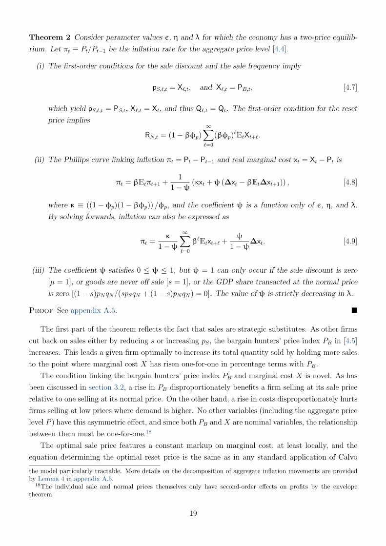
Theorem 2 Consider parameter values ε, η and λ for which the economy has a two-price equilib-
rium. Let πt ≡ Pt/Pt−1 be the inflation rate for the aggregate price level [4.4].
(i) The first-order conditions for the sale discount and the sale frequency imply
pS,`,t = X`,t, and X`,t = PB,t, [4.7]
which yield pS,`,t = PS,t, X`,t = Xt, and thus Q`,t = Qt. The first-order condition for the reset
price implies
RN,t = (1− βφp)∞∑`=0
(βφp)`EtXt+`.
(ii) The Phillips curve linking inflation πt = Pt − Pt−1 and real marginal cost xt = Xt − Pt is
πt = βEtπt+1 +1
1−ψ (κxt +ψ (∆xt − βEt∆xt+1)) , [4.8]
where κ ≡ ((1− φp)(1− βφp)) /φp, and the coefficient ψ is a function only of ε, η, and λ.
By solving forwards, inflation can also be expressed as
πt =κ
1−ψ∞∑`=0
β`Etxt+` +ψ
1−ψ∆xt. [4.9]
(iii) The coefficient ψ satisfies 0 ≤ ψ ≤ 1, but ψ = 1 can only occur if the sale discount is zero
[µ = 1], or goods are never off sale [s = 1], or the GDP share transacted at the normal price
is zero [(1− s)pNqN/(spSqN + (1− s)pNqN) = 0]. The value of ψ is strictly decreasing in λ.
Proof See appendix A.5.
The first part of the theorem reflects the fact that sales are strategic substitutes. As other firms
cut back on sales either by reducing s or increasing pS, the bargain hunters’ price index PB in [4.5]
increases. This leads a given firm optimally to increase its total quantity sold by holding more sales
to the point where marginal cost X has risen one-for-one in percentage terms with PB.
The condition linking the bargain hunters’ price index PB and marginal cost X is novel. As has
been discussed in section 3.2, a rise in PB disproportionately benefits a firm selling at its sale price
relative to one selling at its normal price. On the other hand, a rise in costs disproportionately hurts
firms selling at low prices where demand is higher. No other variables (including the aggregate price
level P ) have this asymmetric effect, and since both PB and X are nominal variables, the relationship
between them must be one-for-one.18
The optimal sale price features a constant markup on marginal cost, at least locally, and the
equation determining the optimal reset price is the same as in any standard application of Calvo
the model particularly tractable. More details on the decomposition of aggregate inflation movements are providedby Lemma 4 in appendix A.5.
18The individual sale and normal prices themselves only have second-order effects on profits by the envelopetheorem.
19

pricing. The optimal adjustment of sales has the consequence that all firms produce the same total
quantity, and thus have the same level of marginal cost.
The Phillips curve with sales in equation [4.8] would reduce to the standard New Keynesian
Phillips curve πt = βEtπt+1 + κxt in the case that ψ = 0.19 On the other hand, the case of a fully-
flexible price level (a vertical short-run Phillips curve) is equivalent to ψ = 1. With parameters
consistent with sales in equilibrium, ψ always lies strictly between these extremes. While varying sale
frequencies and discounts can always generate the same average price change as a given adjustment
of normal prices, in equilibrium, firms never find these to be perfect substitutes and so flexibility in
sales never replicates full price flexility.
The effect of a positive value of ψ is to increase the response of inflation to real marginal cost
to some extent when compared to the New Keynesian Phillips curve. This is best seen by looking
at the solved-forwards version of the Phillips curve with sales in [4.9], where there are two distinct
differences relative to the solved-forwards version of the standard New Keynesian Phillips curve:
πt = κ∑∞
`=0 β`EtXt+`. The first is a scaling of the coefficient multiplying expected real marginal
costs, which is isomorphic to an increase in the probability of price adjustment 1−φp. The second
is the presence of a term in the growth rate of real marginal cost ∆xt. The growth rate appears
in addition to the level because the extra margin of price adjustment operates through temporary
sales rather than persistent changes to normal prices.
The analysis here is based on assumptions congruent with the micro pricing evidence (sticky
normal prices, flexible sales), but are there good reasons for firms to set prices in this way? In
the model, deviations of the sale and normal prices from their profit-maximizing levels would not
be equally costly to firms. Both the price elasticity of demand and the quantity sold at a given
shopping moment are higher at the sale price than at the normal price. This implies that for a
given percentage deviation from their profit-maximizing levels, the benefits from reoptimizing the
sale price would be higher than for the normal price.20
4.3 A DSGE model with sales
This section embeds sales into a dynamic stochastic general equilibrium model with staggered ad-
justment of normal prices and wages.
As in Erceg, Henderson and Levin (2000), firms hire differentiated labour inputs. So hours H in
the production function [2.8] is now the composite labour input
H ≡(∫
H(ı)ς−1
ς dı
) ςς−1
,
where H(ı) is hours of type-ı labour supplied to a given firm, and ς is the elasticity of substitution
between labour types. It is assumed that ς > 1, and firms are price takers in the markets for labour
inputs. The minimum monetary cost of hiring one unit of the composite labour input H is denoted
19See Woodford (2003) for a derivation and discussion of the standard New Keynesian Phillips curve.20This point is discussed further in an earlier working paper (Guimaraes and Sheedy, 2008).
20

by W , and this is now the relevant wage index appearing in firms’ cost function [2.9].
Each household (supplying a particular type of labour) has a probability 1−φw of being able to
adjust its money wage in any given time period. Since households have equal initial financial wealth
and expected lifetime income, as asset markets are complete and utility [2.1] is additively separable
between hours and consumption, households are fully insured and hence have equal consumption
in equilibrium. Consumption is the only source of expenditure, so goods market equilibrium re-
quires Ct = Yt. Thus by using [2.3] and [2.4], and by noting that [2.2b] is binding, the following
intertemporal IS equation and money-market equilibrium condition are obtained:
β(1 + it)Et
[υc(Yt+1)
υc(Yt)
1
πt+1
]= 1, and Yt =
Mt
Pt. [4.10]
The wage setting and wage index equations are as in Erceg, Henderson and Levin (2000).21
Finally, the model is closed by specifying a rule for monetary policy. The growth rate of the
money supply Mt is assumed to follow the first-order autoregressive process
Mt
Mt−1
=
(Mt−1
Mt−2
)p
exp (1− p)et , where et ∼ i.i.d.(0, Ωm). [4.11]
4.4 Calibration
The distinguishing parameters of the sales model are the two elasticities ε and η and the fraction λ
of loyal customers. As shown in Proposition 1, these parameters are directly related to observable
prices and quantities: the markup ratio µ, which gives the size of the discount offered when a good
is on sale; the quantity ratio χ, which measures proportionately how much more is purchased when
a good is on sale; and the frequency of sales s. Furthermore, the model has a convenient block
recursive structure in that only ε, η and λ need to be known to determine these observables. There
are thus three parameters that can be matched to data on just these three variables.22
There is a growing empirical literature examining price adjustment patterns at the microeconomic
level. This literature provides information about the markup ratio µ and the sales frequency s. The
baseline values of these variables are taken from Nakamura and Steinsson (2008). Their study draws
on individual price data from the BLS CPI research database, which covers approximately 70% of
U.S. consumer expenditure. They report that the fraction of price quotes that are sales (weighted
by expenditure) is 7.4%, so s = 0.074 is used here.23 They also report that the median difference
between the logarithms of the normal and sale prices is 0.295, which yields µ = 0.745.
In the retail and marketing literature, there has been for a long time a discussion of the effects of
price promotions on demand. This research provides information about the quantity ratio. Papers
typically report a range of estimates conditional on factors other than price that affect the impact
21See appendix A.6 for details of these equations.22It is also possible to match these three parameters using data on the average markup instead of the quantity
ratio. This approach would be in line with typical practice in macroeconomics, but the strategy adopted here is moredirect.
23The sales frequency s is for the whole economy. Certain sectors have higher frequencies of sales and some sectorshave none. The implications of such heterogeneity are considered in section 5.
21

of a price promotion, for example, advertising. The baseline value of the quantity ratio is obtained
from the study by Narasimhan, Neslin and Sen (1996). Their results are based on scanner data from
a large number of U.S. supermarkets. According to the elasticities they report, a temporary price
cut of the size consistent with the sale discount taken from Nakamura and Steinsson (2008) implies
a quantity ratio of between approximately 4 and 6 if retailers draw their sale to the attention of
customers. The baseline number used here is the midpoint of this range, so χ = 5.24
The three facts about sales are then used to find matching values of the three unknown param-
eters.25 The results are shown in Table 1.
Table 1: Calibration of the model of sales
Description Notation Value
Stylized factsRatio of the sale-price markup to the normal-price markup (µS/µN) µ 0.745*
Ratio of quantities sold at the sale price and the normal price (qS/qN) χ 5†
Frequency of sales s 0.074*
ParametersElasticity of substitution between product types ε 3.01Elasticity of substitution between brands for a bargain hunter η 19.7Fraction of product types for which a household is loyal to a brand λ 0.901
Notes: These parameters are the only values exactly consistent with the three stylized facts about sales.* Source: Nakamura and Steinsson (2008)† Source: Narasimhan, Neslin and Sen (1996)
The remainder of the calibration is standard, drawing on conventional values from the DSGE
literature. The parameter values selected are shown in Table 2. One time period corresponds to one
month. The discount factor β is chosen to yield a 3% annual real interest rate, the intertemporal
elasticity of substitution in consumption θc is chosen to match a coefficient of relative risk aversion
of 3, and the Frisch elasticity of labour supply θh is set to 0.7, which lies in the range of estimates
found in the literature (Hall, 2009). The production function is F(H) = AHα, where α is the
elasticity of output with respect to hours. The value of α is chosen to match a labour share of 0.667.
This production function implies that the elasticity γ of marginal cost with respect to output is
given by γ = (1−α)/α. So α = 0.667 yields γ = 0.5. The elasticity of substitution between labour
inputs ς is taken from Christiano, Eichenbaum and Evans (2005). The probability φp of stickiness
of the normal price is set to match an average price-spell duration of 9 months, which is taken from
Nakamura and Steinsson (2008). The same number is used for the probability of wage stickiness φw,
24This quantity ratio is very close to what would be consistent with a price elasticity of 6 over the relevant rangeof the demand function. Levin and Yun (2009) find that substitution by consumers on the extensive margin betweenbrands alone can account for elasticities of approximately this size.
25A procedure for calculating the equilibrium values of µ, χ, and s is described in appendix A.1. Given the mappingfrom parameters to the equilibrium of the model, parameters matching the three stylized facts were found by applyingthe Nelder-Mead simplex algorithm. An extensive grid search over the elasticities ε and η was used to verify thatno other values are consistent with the targets for µ and χ. Proposition 1 demonstrates that given ε and η, there isalways one and only one value of λ matching the target sales frequency s.
22

as evidence shows that most, but not all, wages are adjusted annually. The persistence parameter of
money-supply growth p is chosen to match the first-order autocorrelation coefficient of M1 growth
in the U.S. from 1960:1 to 1999:12.
Table 2: Calibration of the DSGE model parameters
Description Notation Value
Preference parametersSubjective discount factor β 0.9975Intertemporal elasticity of substitution in consumption θc 0.333Frisch elasticity of labour supply θh 0.7†
Technology parametersElasticity of output with respect to hours α 0.667Elasticity of marginal cost with respect to output γ 0.5Elasticity of substitution between differentiated labour inputs ς 20‡
Nominal rigiditiesProbability of stickiness of normal prices φp 0.889§
Probability of wage stickiness φw 0.889
Monetary policyFirst-order serial correlation of the money-supply growth rate p 0.536]
Notes: Monthly calibration.† Source: Hall (2009)‡ Source: Christiano, Eichenbaum and Evans (2005)§ Source: Nakamura and Steinsson (2008)] Source: Authors’ calculations using data on M1 for the period 1960:1–1999:1. Series M1SL from
Federal Reserve Economic Data (http://research.stlouisfed.org/fred2).
4.5 Dynamic simulations
This section calculates the impulse responses of output and the price level to monetary policy
shocks in the calibrated DSGE model with sales. These are compared to the corresponding impulse
responses in a standard DSGE model, that is, one where consumers have regular Dixit-Stiglitz pref-
erences and thus firms employ a one-price strategy, and where price-adjustment times are staggered
according to the Calvo (1983) model. With Calvo pricing, a standard New Keynesian Phillips curve
is obtained. The latter model is set up so that it is otherwise identical to the DSGE model with
sales.
The calibrated parameters of the DSGE model with sales are given in Table 1 and Table 2. For
the standard DSGE model without sales, the same parameter values from Table 2 are used, with the
probability of price stickiness φp applying to a firm’s single price, rather than to its normal price in
the sales model. In place of the parameters ε, η and λ, the standard model requires only a calibration
of its constant price elasticity of demand ξ (the elasticity of substitution in the usual Dixit-Stiglitz
23

aggregator). This is chosen to match the average markup (in the sense of the reciprocal of real
marginal cost) from the calibrated sales model. For the baseline calibration this implies ξ = 3.77.
Figure 5: Impulse responses to a persistent shock to money growth
Output
%
Standard modelSales model
Price level
Months
%
0 5 10 15 20 25 30 35 40 45
0 5 10 15 20 25 30 35 40 45
0
0.2
0.4
0.6
0.8
1
0
0.2
0.4
0.6
0.8
Notes: The model is as described in section 4. Parameter values are given in Table 1 and Table 2.
Figure 5 plots the impulse response functions of aggregate output and the price level to a serially-
correlated money growth shock in both the sales model and the standard model without sales. The
real effects of monetary policy in the model with sales are large and very similar to those found in
the standard model, in spite of firms’ full freedom to react to the shock by varying sales without
cost. The ratio of the cumulated responses of output between the two models is 0.89. Underlying
this finding is the modest reaction of sale discounts and the neglible reaction of sales frequencies to
the shock.26
Strategic substitutability in sales decisions is fundamental to understanding the real effects of
monetary policy in the sales model. On the one hand, firms have an incentive to reduce sales in
response to a positive monetary shock, essentially mimicking an increase in price. On the other
hand, owing to strategic substitutability in sales, as other firms reduce their sales, an individual
firm has a strong incentive to target the bargain hunters, who are being neglected by others. Thus
26The impulse responses of the average sale discount and the average sale frequency are both proportional to thatof real marginal cost, as shown in Lemma 4.
24

there are two conflicting effects on sales and the price level after a monetary shock. One tends
towards money neutrality, while the other tends towards money having real effects.
Quantitatively, finding the right balance between targeting their two groups of customers turns
out to be much more important to firms’ profits than using sales as a means of changing their
average prices. In the data, there is a substantial gap between sale and normal prices on average.
So a relatively modest response of sales to a monetary shock would suffice to raise the price level in
line with the money supply. However, the larger the gap between the two prices, the greater must be
the difference between the two customer types in terms of their price sensitivities, which increases
the incentives for a contrarian response to other firms’ pricing strategies. This strong strategic
substitutability dissuades firms from adjusting sales because all firms would need to respond in the
same way to the aggregate monetary shock.27
The role of strategic substitutability can be isolated by considering instead an idiosyncratic
demand shock to one single firm. Since this one firm is negligible, no other firms react, so the bargain
hunters’ price index PB does not change. From the first-order condition in [4.7], the marginal cost of
the affected firm must remain unchanged. Hence, the total quantity the firm produces is insulated
from the demand shock through its adjustment of sales. This is in stark contrast to the small
response of sales to aggregate demand shocks where strategic considerations dominate.
The robustness of these results is checked by performing a sensitivity analysis with respect to
the key empirical targets used to calibrate the model: the markup ratio, the quantity ratio, and the
sales frequency. A range of values for each around its baseline value from Table 1 is considered. One
target is varied at a time while the others are held constant. The sensitivity analysis is extended to
include the elasticity of output with respect to hours to explore the implications of different degrees
of curvature of firms’ cost functions.
Figure 6 depicts the ratio of the cumulated impulse response of output in the model with sales
to that in the standard model as a function of each target, performing exactly the same monetary
policy experiment described earlier.
The impulse responses are not particularly sensitive to the calibration targets. The quantity
ratio χ is the target for which the literature yields the widest range of estimates. But nonetheless,
varying χ from 2 to 8 implies that the ratio of cumulated output responses lies only between 0.87
and 0.9. For the other targets, more precise data are available. By considering markup ratios from
0.65 to 0.85 (a wide band around the baseline value), the response ratio between the models varies
from 0.84 to 0.91. Similarly, a wide range of sales frequencies from 0.05 to 0.15 yields ratios between
0.86 and 0.9.
Finally, for values of the elasticity of output with respect to hours above the baseline, all the
way up to one, the ratio of cumulated output responses is higher than 0.89. In particular, as the
27Although firms’ sales are reacting only slightly to monetary shocks, the losses from failing to adjust the normalprice more frequently are considerably smaller than they would otherwise be in a model without sales. The possibilityof adjusting sales implies that the quantity produced by an individual firm would be exactly the same had this firmthe option of adjusting its normal price in addition to adjusting its sales, as is shown in Theorem 2. Hence there areno undesirable fluctuations in marginal cost, and so the further gains from adjusting the normal price are smaller.This point is discussed further in an earlier working paper (Guimaraes and Sheedy, 2008).
25

Figure 6: Sensitivity analysis for the real effects of monetary shocks
Markup ratio (µ)
Ratio of cumulative output responses
Quantity ratio (χ)
Sales fraction (s)
Elasticity of output with respect to hours (α)0.65 0.7 0.75 0.8 0.85 0.9 0.95
0.05 0.1 0.15 0.2
3 4 5 6 7
0.65 0.7 0.75 0.8 0.85
0.8
0.9
0.8
0.9
0.8
0.9
0.8
0.9
Notes: For each graph, the results are obtained by fixing the other targets at their baseline values asgiven in Table 1 (together with α = 2/3) and choosing matching values of the parameters ε, η and λas explained in section 4.4.
elasticity gets close to one, the ratio approaches 0.99. This implies that when the cost function is
close to being linear, the real effects of monetary policy are essentially the same in the model with
fully flexible sales as in the standard model with no sales at all.
The intuition for this finding is that when the cost function is linear, marginal cost does not
26

depend on the quantity of output produced. So a rise in aggregate demand, which if accommodated
would increase the quantity sold, no longer provides firms with a reason to reduce sales. Hence all
that matters for sales decisions is striking the right balance between targeting loyal customers and
bargain hunters.
Figure 7: A typical individual price path generated by the model
Time10 20 30 40 50 60 70 80 90
0.80
0.90
1.00
Notes: Obtained using the baseline calibration of the DSGE model with sales and the money supplyfollowing a random walk with drift. The initial normal price is set to 1.
Figure 7 shows an example of an individual price path in the model with sales generated using
the baseline calibration. Price observations are sampled at a weekly frequency. The underlying
stochastic process for the money supply is a random walk with drift. The behaviour depicted is
qualitatively and quantitatively consistent with real-world examples of prices without needing to
assume any idiosyncratic shocks are present.28
It is interesting to note from Figure 7 that the model can explain the coexistence of both small
and large price changes for the same product in the presence of only macroeconomic shocks. Without
any shocks at all, sales would still occur at a very similar frequency, but individual prices would
switch between unchanging normal and sale prices.
Behind the findings of this section lies the fact that the equilibrium distribution of prices reacts
little to monetary shocks. So while the occurrence of sales means that there is much more nominal
flexibility of individual prices, the rationale for sales implies that there is an endogenous real rigidity
constraining the adjustment of the relative prices in firms’ price distributions.
5 Sectoral heterogeneity in sales
The model presented thus far assumes all sectors of the economy have the same pattern of sales.
But sales are in fact concentrated in some sectors, and rare or non-existent in others. This creates
28The model can be reinterpreted in terms of producers choosing a distribution of prices across a continuum ofretail outlets, with each outlet maintaining the same price during each discrete time period. In this case, Figure 7corresponds to the price path at a randomly chosen outlet.
27
a divergence between estimates of the frequency of sales using data covering the whole economy
(Nakamura and Steinsson, 2008) and those based on scanner data from supermarkets. These findings
suggest a multi-sector model is more empirically appropriate for analysing the implications of sales.
The model of section 2 is extended to include two sectors. In one sector, households have homo-
geneous Dixit-Stiglitz preferences over brands of product types, so no sales will occur in equilibrium.
In the other sector, household preferences over brands are heterogeneous, with some mixture of loyal
and bargain hunting behaviour, which will give rise to sales in equilibrium. This extension is simple
and tractable.
A measure σ of product types are in the sale sector, with T now denoting the set of just these
product types, and where household preferences are as described in section 2. The remaining set
of product types with measure 1 − σ in the non-sale sector is denoted by H . The new composite
good C replacing that in equation [2.5] is
C ≡(∫
Λ
c(τ,B(τ))ε−1
ε dτ+
∫T \Λ
(∫B
c(τ, b)η−1
η db
)η(ε−1)ε(η−1)
dτ+
∫H
(∫B
c(τ, b)ξ−1
ξ db
)ξ(ε−1)ε(ξ−1)
dτ
) εε−1
,
[5.1]
where ξ is the homogeneous elasticity of substitution between brands in the non-sale sector for all
households.
Two restrictions are imposed. First, the elasticity ξ is chosen to ensure the markup in the non-
sale sector is equal to the economy’s average markup (in the sense of the reciprocal of real marginal
cost). This entails choosing ξ = 1/(1 − x), where x is calculated for the sale sector as in [3.8], as
if it encompassed the whole economy. Second, the relative contributions of the sale and non-sale
sectors to GDP must be proportional to σ and 1 − σ. Given that the sale sector features price
distortions, it is not possible to satisfy these two restrictions when the production function is the
same in both sectors. Consequently, a slight adjustment is made to the non-sale sector production
function F(H), but one which ensures it has the same elasticity of output with respect to hours α
and elasticity of marginal cost with respect to output γ as the production function F(H) in the sale
sector. These conditions are satisfied only when F(H) = ∆F(∆−1H), where ∆ is the stationary
equilibrium price distortion (ratio of Y to Q) in the sale sector from [3.10] (again, calculated as
if this sector encompassed the whole economy). Since ∆ is close to one in practice, the difference
between the production functions is very small.
The characteristics of a sale when one occurs (the discount size, and the extra amount purchased)
are the same here as in the earlier one-sector model. Proposition 1 shows that the markup ratio
µ and the quantity ratio χ depend solely on the elasticities ε and η. So neither µ and χ, nor ε
and η, change when moving from the one-sector to the two-sector model. The two-sector model
allows for the sale sector to have an above-average frequency of sales s, while holding constant the
average sales frequency s = σs for the whole economy. The higher frequency within the sale sector
is matched by a lower value of λ there than in the one-sector model. Finally, the extent of nominal
rigidity (excluding sales) is equal across sectors, in the sense that price stickiness in the non-sale
sector is the same as normal-price stickiness in the sale sector.
28

Proposition 2 Let Ψ(s; ε,η) be the Phillips curve coefficient ψ from Theorem 2 implied by a sale
frequency s, with parameters ε and η consistent with µ and χ, and with λ implicitly adjusted to
match s, as if the sale sector encompassed the whole economy.
(i) The function Ψ(s; ε,η) is strictly increasing and strictly concave in s.
(ii) In the case of constant marginal cost (γ = 0), the Phillips curve for aggregate inflation in the
two-sector model is of exactly the same form as that in Theorem 2 with ψ replaced by the
weighted average of Ψ(s; ε,η) (for the sale sector) and 0 (for the non-sale sector) using weights
σ and 1− σ. This weighted average is less than Ψ(σs; ε,η) for all σ < 1.
Proof See appendix A.8.
The first finding states that Ψ(s; ε,η), which can be interpreted as the amount of price-level
flexibility resulting from adjustment of sales, is increasing in the frequency with which sales occur,
but at a diminishing rate. In a multi-sector context, what matters for aggregate price flexibility
is mainly the weighted average of the value of ψ across sectors. Therefore, by Jensen’s inequality,
an economy with an unequal distribution of sales across sectors implies a lower average value of ψ,
and thus a flatter aggregate Phillips curve where monetary policy has larger real effects, than an
economy with just one sector, but the same average sales frequency. The second finding makes this
intuition precise when marginal cost is constant.29
Table 3: Calibration of the two-sector model
Description Notation Value
Stylized factsFrequency of sales in the sale sector s 0.29*
Aggregated frequency of sales s 0.074†
ParametersFraction of loyal customers for each brand in the sale sector λ 0.735Size of the sale sector σ 0.255
Notes: The stylized facts for µ and χ are as in Table 1 along with the matching parametersvalues for ε and η.
* Source: Eichenbaum, Jaimovich and Rebelo (2008)† Source: Nakamura and Steinsson (2008)
The two-sector model is now calibrated to establish the magnitude of the effect of sectoral
heterogeneity on the earlier findings. The only change to the earlier calibration is that the sale
frequency in the sale sector s is targeted in addition to the average sale frequency s for the whole
economy. The two targets are matched by adjusting λ and σ appropriately.
Eichenbaum, Jaimovich and Rebelo (2008) study data from a major U.S. retailer and find that
prices are below their “reference” level 29% of the time on average. Hence, the target value for s is
29The equations of the two-sector model in the general case γ 6= 0 are presented in appendix A.7. The analysis caneasily be extended to an n-sector model.
29

Figure 8: Impulse responses to a persistent shock to money growth in the two-sector model
Output
%
Standard modelSales model
Price level
Months
%
0 5 10 15 20 25 30 35 40 45
0 5 10 15 20 25 30 35 40 45
0
0.2
0.4
0.6
0.8
0
0.2
0.4
0.6
0.8
Notes: The model is as described in section 5. Parameter values are from Table 2 and Table 3.
0.29, which yields σ, the size of the sale sector, equal to 0.255 when the economy-wide sale frequency
must be the same as the one-sector calibration (Table 1). The calibration exercise is summarized in
Table 3.
Figure 8 shows the impulse responses to the same monetary policy experiment described in
section 4 for the two-sector model with sales and the standard model without any sales. The
difference between the impulse responses is even smaller than before. The ratio of the cumulated
responses of output is now 0.96, in contrast to 0.89 in the one-sector model. This shows that sales
are essentially irrelevant for monetary policy analysis in the two-sector model.
6 Conclusions
For macroeconomists grappling with the welter of recent micro pricing evidence, one particularly
puzzling feature is noteworthy: the large, frequent and short-lived price cuts followed by prices
returning exactly to their former levels. If price changes are driven purely by shocks then explaining
this tendency requires a very special configuration of shocks. The model presented in this paper
shows that just such pricing behaviour arises in equilibrium if firms face consumers with sufficiently
30

different price sensitivities.
The model proposed in this paper is used to understand the implications for monetary policy
analysis of flexibility in sales alongside stickiness in normal prices. Explaining the occurrence of sales
in a framework based on consumer heterogeneity entails strategic substitutability of sales decisions.
But it is exactly because sales are strategic substitutes that they barely react to aggregate shocks,
including monetary policy shocks. This is in spite of firms having a direct incentive to adjust
sales when their normal prices are sticky. Firms would adjust sales in response to idiosyncratic
shocks: only aggregate shocks lead to a tension between adjustment through sales and strategic
considerations.
The findings of this paper indicate that in a world with both sticky normal prices and flexible
sales, it is stickiness in the normal price that matters so far as monetary policy analysis is concerned.
Arriving at this conclusion requires a careful modelling of the reasons why sales occur. Thus the
results highlight the importance for macroeconomics of understanding what lies behind firms’ pricing
decisions.
References
Bils, M. and Klenow, P. J. (2004), “Some evidence on the importance of sticky prices”, Journal
of Political Economy, 112(5):947–985 (October). 1, 14
Calvo, G. A. (1983), “Staggered prices in a utility-maximizing framework”, Journal of Monetary
Economics, 12(3):383–398 (September). 17, 23
Christiano, L. J., Eichenbaum, M. and Evans, C. L. (2005), “Nominal rigidities and the
dynamic effects of a shock to monetary policy”, Journal of Political Economy, 113(1):1–45 (Febru-
ary). 22, 23
Dhyne, E., Alvarez, L. J., Le Bihan, H., Veronese, G., Dias, D., Hoffmann, J.,
Jonker, N., Lunnemann, P., Rumler, F. and Vilmunen, J. (2006), “Price changes in
the euro area and the United States: Some facts from individual consumer price data”, Journal
of Economic Perspectives, 20(2):171–192 (Spring). 1
Eichenbaum, M., Jaimovich, N. and Rebelo, S. (2008), “Reference prices and nominal rigidi-
ties”, Working paper 13829, National Bureau of Economic Research. 1, 29
Erceg, C. J., Henderson, D. W. and Levin, A. T. (2000), “Optimal monetary policy with
staggered wage and price contracts”, Journal of Monetary Economics, 46(2):281–313 (October).
20, 21, 58
Goldberg, P. and Hellerstein, R. (2007), “A framework for identifying the sources of local-
currency price stability with an empirical application”, Working paper 13183, National Bureau
of Economic Research. 1
31

Guimaraes, B. and Sheedy, K. D. (2008), “Sales and monetary policy”, Discussion paper 6940,
Centre for Economic Policy Research. 20, 25
Hall, R. E. (2009), “Reconciling cyclical movements in the marginal value of time and the marginal
product of labor”, Journal of Political Economy, 117(2):281–323 (April). 22, 23
Hosken, D. and Reiffen, D. (2004), “Patterns of retail price variation”, RAND Journal of
Economics, 35(1):128–146 (Spring). 1
Kehoe, P. J. and Midrigan, V. (2008), “Temporary price changes and the real effects of mon-
etary policy”, Working paper 14392, National Bureau of Economic Research. 1, 3, 13
Kimball, M. S. (1995), “The quantitative analytics of the basic Neomonetarist model”, Journal
of Money, Credit and Banking, 27(4 part 2):1241–1277 (November). 9
Klenow, P. J. and Kryvtsov, O. (2008), “State-dependent or time-dependent pricing: Does it
matter for recent U.S. inflation?”, Quarterly Journal of Economics, 123(3):863–904. 1
Lazear, E. P. (1986), “Retail pricing and clearance sales”, American Economic Review, 76(1):14–
32 (March). 14
Levin, A. and Yun, T. (2009), “Reconsidering the microeconomic foundations of price-setting
behavior”, Working paper, Federal Reserve Board. 22
Nakamura, E. (2008), “Pass-through in retail and wholesale”, American Economic Review,
98(2):430–437 (May). 13
Nakamura, E. and Steinsson, J. (2008), “Five facts about prices: A reevaluation of menu cost
models”, Quarterly Journal of Economics, 123(4):1415–1464 (November). 1, 14, 21, 22, 23, 28,
29
——— (2009), “Price setting in forward-looking customer markets”, Working paper, Columbia
University. 13
Narasimhan, C. (1988), “Competitive promotional strategies”, Journal of Business, 61(4):427–
449 (October). 2, 13
Narasimhan, C., Neslin, S. and Sen, S. (1996), “Promotional elasticities and category char-
acteristics”, Journal of Marketing, 60(2):17–30 (April). 22
Neslin, S. A. (2002), “Sales promotion”, in Handbook of Marketing, SAGE. 13
Salop, S. and Stiglitz, J. E. (1977), “Bargains and ripoffs: A model of monopolistically com-
petitive price dispersion”, Review of Economic Studies, 44(3):493–510 (October). 1
——— (1982), “The theory of sales: A simple model of equilibrium price dispersion with identical
agents”, American Economic Review, 72(5):1121–1130 (December). 2
32
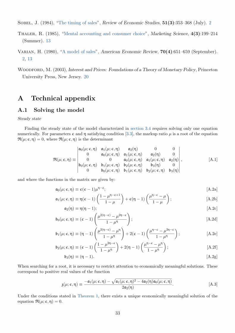
Sobel, J. (1984), “The timing of sales”, Review of Economic Studies, 51(3):353–368 (July). 2
Thaler, R. (1985), “Mental accounting and consumer choice”, Marketing Science, 4(3):199–214
(Summer). 13
Varian, H. (1980), “A model of sales”, American Economic Review, 70(4):651–659 (September).
2, 13
Woodford, M. (2003), Interest and Prices: Foundations of a Theory of Monetary Policy, Princeton
University Press, New Jersey. 20
A Technical appendix
A.1 Solving the model
Steady state
Finding the steady state of the model characterized in section 3.4 requires solving only one equationnumerically. For parameters ε and η satisfying condition [3.3], the markup ratio µ is a root of the equationR(µ; ε,η) = 0, where R(µ; ε,η) is the determinant
R(µ; ε,η) ≡
∣∣∣∣∣∣∣∣∣∣a0(µ; ε,η) a1(µ; ε,η) a2(η) 0 0
0 a0(µ; ε,η) a1(µ; ε,η) a2(η) 00 0 a0(µ; ε,η) a1(µ; ε,η) a2(η)
b0(µ; ε,η) b1(µ; ε,η) b2(µ; ε,η) b3(η) 00 b0(µ; ε,η) b1(µ; ε,η) b2(µ; ε,η) b3(η)
∣∣∣∣∣∣∣∣∣∣, [A.1]
and where the functions in the matrix are given by:
a0(µ; ε,η) ≡ ε(ε− 1)µη−ε; [A.2a]
a1(µ; ε,η) ≡ η(ε− 1)(
1− µη−ε+1
1− µ
)+ ε(η− 1)
(µη−ε − µ
1− µ
); [A.2b]
a2(η) ≡ η(η− 1); [A.2c]
b0(µ; ε,η) ≡ (ε− 1)
(µ2(η−ε) − µ2η−ε
1− µη
); [A.2d]
b1(µ; ε,η) ≡ (η− 1)
(µ2(η−ε) − µη
1− µη
)+ 2(ε− 1)
(µη−ε − µ2η−ε
1− µη)
; [A.2e]
b2(µ; ε,η) ≡ (ε− 1)(
1− µ2η−ε
1− µη)
+ 2(η− 1)(µη−ε − µη
1− µη)
; [A.2f]
b3(η) ≡ (η− 1). [A.2g]
When searching for a root, it is necessary to restrict attention to economically meaningful solutions. Thesecorrespond to positive real values of the function
z(µ; ε,η) ≡ −a1(µ; ε,η)−√
a1(µ; ε,η)2 − 4a2(η)a0(µ; ε,η)2a2(η)
. [A.3]
Under the conditions stated in Theorem 1, there exists a unique economically meaningful solution of theequation R(µ; ε,η) = 0.
33

Having obtained the markup ratio µ, the quantity ratio χ is
χ = µ−ε(
1 + µ−(η−ε)z(µ; ε,η)1 + z(µ; ε,η)
), [A.4]
and the sales frequency s is
s =
(λ
1−λz(µ; ε,η))−( η−1
η−ε
)− 1
µ−(η−1) − 1. [A.5]
This expression for the sales frequency is economically meaningful when λ lies between the bounds λ(ε,η)and λ(ε,η) referred to in Theorem 1, which are given by:
λ(ε,η) ≡ 11 + µ−(η−ε)z (µ; ε,η)
, and λ(ε,η) ≡ 11 + z (µ; ε,η)
. [A.6]
An expression for real marginal cost x (the reciprocal of the average markup) is
x =(λ((1 + z (µ; ε,η)) +
((µ1−ε − 1) + (µ1−η − 1)z (µ; ε,η)
)s)) 1
ε−1
((ε− 1) + (η− 1)z (µ; ε,η)
ε+ ηz (µ; ε,η)
), [A.7]
and the degree of price distortion ∆ = Y/Q is given by:
∆ =
(λ((1 + z (µ; ε,η)) +
((µ1−ε − 1) + (µ1−η − 1)z (µ; ε,η)
)s)) ε
ε−1
λ ((1 + z (µ; ε,η)) + ((µ−ε − 1) + (µ−η − 1)z (µ; ε,η)) s). [A.8]
DSGE model
The system of log-linearized equations of the model from section 4 is
πt = βEtπt+1 +1
1−ψ (κxt +ψ (∆xt − βEt∆xt+1)) ; [A.9a]
xt =1
1 + γδwt +
γ
1 + γδYt; [A.9b]
πW,t = βEtπW,t+1 +(1− φw)(1− βφw)
φw
11 + ςθ−1
h
((θ−1c +
11 + γδ
θ−1h
α
)Yt −
(1 +
δ
1 + γδθ−1h
α
)wt
);
[A.9c]
∆wt = πW,t − πt; [A.9d]Yt = EtYt+1 − θc (it − Etπt+1) ; [A.9e]
∆Yt = ∆Mt − πt; [A.9f]∆Mt = p∆Mt−1 + (1− p)et. [A.9g]
The Phillips curve equation is from Theorem 2 and derivations of the other equations are given in appendixA.6. All the coefficients apart from ψ, κ and δ are as defined in Table 2. Formulæ for ψ, κ and δ are
ψ = 1−(1− s)
(1−
(η−1ε−1
)(µ1−ε−1µ1−η−1
))(1 + z(µ; ε,η)) + ((µ1−ε − 1) + (µ1−η − 1)z(µ; ε,η)) s
, κ =(1− φp)(1− βφp)
φp, and [A.10a]
δ =sχε(1− µ)sχ+ (1− s) [A.10b]
+sχµ+ (1− s)sχ+ (1− s)
1ε−1
((ε− 1)(µ−ε − 1)− ε(µ1−ε − 1)
)+ z(µ;ε,η)
η−1
((η− 1)(µ−η − 1)− η(µ1−η − 1)
)(µ1−η−1η−1
)−(µ1−ε−1ε−1
) .
34

The solution of the system [A.9] can be obtained using standard methods for solving expectational differenceequations.
The standard model without sales is a special case of [A.9] with the following parameter restrictions:
ψ = 0, δ = 0, ξ =1
1− x, and κ =1
1 + ξγ(1− φp)(1− βφp)
φp,
where the Phillips curve then reduces to the standard New Keynesian Phillips curve.
A.2 Properties of the demand, revenue and marginal revenue functions
The structure of household consumption preferences introduced in section 2.2 implies that firms face ademand curve q = D(p;PB, E) of the form given in equation [2.10] at each shopping moment. It is easier toanalyse the properties of this demand function — and the associated total and marginal revenue functions— by working with what can be thought of as the corresponding “relative” demand function D(ρ), definedby
D(ρ) ≡ λρ−ε + (1− λ)ρ−η, [A.11]
which satisfies D(1) = 1 for all choices of parameters. The relative demand function q = D(ρ) gives the“relative” quantity sold q as a function of the relative price ρ, where relative price here means money pricep relative to PB, the bargain hunters’ price index from [2.7], and relative quantity means quantity q soldrelative to E/P εB, where E = P εY is the measure of aggregate expenditure from [2.10]:
ρ ≡ p
PB, and q ≡ P εB
E q. [A.12]
With these definitions, the original demand function [2.10] is stated in terms of the relative demand function[A.11] as follows:
D(p;PB, E) =EP εBD(p
PB
). [A.13]
The relative demand function [A.11] is a continuously differentiable function of ρ for all ρ > 0, andis strictly decreasing everywhere. Notice also that D(ρ) → ∞ as ρ → 0, and D(ρ) → 0 as ρ → ∞. Bycontinuity and monotonicity, this implies that for every q > 0 there is a unique ρ > 0 such that q = D(ρ).Thus the inverse demand function D−1(q) is well defined for all q > 0, and is itself strictly decreasing andcontinuously differentiable. The revenue function R(q), defined in terms of the relative demand function,is
R(q) ≡ qD−1(q). [A.14]
Using the inverse demand function ρ = D−1(q), an equivalent expression for the revenue function is R(q) =D−1(q)D
(D−1(q)
), and by substituting the demand function from [A.11]:
R(q) = λ(D−1(q)
)1−ε + (1− λ)(D−1(q)
)1−η.
Since ε > 1 and η > 1, and given the limiting behaviour of the demand function established above, itfollows that R(q) → ∞ as q → ∞ and R(q) → 0 as q → 0. Hence, R(0) = 0, and R(q) is continuouslydifferentiable for all q ≥ 0.
Differentiating the revenue function R(q) from [A.14] using the inverse function theorem, and substi-tuting demand function [A.11] yields an expression for marginal revenue:
R′ (D(ρ)) =(
(ε− 1)λ+ (η− 1)(1− λ)ρε−η
ελ+ η(1− λ)ρε−η
)ρ. [A.15]
Because ε > 1 and η > 1, it follows that R′(q) > 0 for all q, so revenue R(q) is strictly increasing in q.Furthermore, because ρ → ∞ as q → 0, and ρ → 0 as q → ∞, [A.15] implies R′(q) → ∞ as q → 0 andR′(q)→ 0 as q→∞.
35

Just as [A.13] establishes the original demand function D(p;PB, E) in [2.10] is connected to the relativedemand function D(ρ) in [A.11], there are similar relations between the original inverse demand functionD−1(q;PB, E), original revenue R(q;PB, E) and marginal revenue R′(q;PB, E) functions, and their equiv-alents defined in terms of the relative demand function. The link between the inverse demand functionsfollows directly from [A.13]:
D−1(q;PB, E) = PBD−1
(qP εBE
). [A.16]
Equations [2.11], [A.14] and [A.16] justify the following connections between the revenue functions andtheir derivatives:
R(q;PB, E) = P 1−εB ER
(qP εBE
), R′(q;PB, E) = PBR′
(qP εBE
), and R′′(q;PB, E) =
P 1+εB
E R′′(qP εBE
).
[A.17]The next result examines the conditions under which marginal revenue R′(q) is non-monotonic.
Lemma 1 Consider the marginal revenue function R′(q) obtained from [A.14] using the relative demandfunction [A.11], and suppose that η > ε > 1.
(i) If λ = 0 or λ = 1 or condition [3.3] does not hold then marginal revenue R′(q) is strictly decreasingfor all q ≥ 0.
(ii) If 0 < λ < 1 and ε and η satisfy condition [3.3] then there exist q and q such that 0 < q < q < ∞and where R′(q) is strictly decreasing between 0 and q and above q, and strictly increasing betweenq and q.
Proof (i) If λ = 0 then it follows from [A.15] that R′(q) = ((η − 1)/η)D−1(q), and if λ = 1 thatR′(q) = ((ε− 1)/ε)D−1(q). Since the inverse demand function D−1(q) is strictly decreasing, then marginalrevenue must also be so in these cases.
(ii) In what follows, assume 0 < λ < 1. Differentiate [A.15] to obtain
D′(ρ)R′′ (D(ρ)) =η(η− 1)
(1−λλρε−η
)2 − ((η− ε)2 − η(ε− 1)− ε(η− 1)) ( (1−λ)
λρε−η
)+ ε(ε− 1)(
ε+ η(
1−λλρε−η
))2 ,
[A.18]for all ρ > 0, where the assumption that λ 6= 0 is used to simplify the expression by dividing through byλ2. Define the function Z(q) in terms of inverse demand function D−1(q):
Z(q) ≡ 1− λλ
(D−1(q)
)ε−η, [A.19]
and use this together with [A.18] to write the derivative of marginal revenue as follows:
R′′(q) =η(η− 1) (Z(q))2 −
((η− ε)2 − η(ε− 1)− ε(η− 1)
)Z(q) + ε(ε− 1)
D′ (D−1(q)) (ε+ ηZ(q))2 . [A.20]
Since D′(D−1(q)
)< 0 for all q, and the remaining term in the denominator of [A.20] is strictly positive,
the sign of R′′(q) is the opposite of that of the quadratic function
Q(z) ≡ η(η− 1)z2 −((η− ε)2 − η(ε− 1)− ε(η− 1)
)z + ε(ε− 1), [A.21]
evaluated at z = Z(q). The aim is to find a region where marginal revenue is upward sloping, whichcorresponds to Q(z) being negative, which is in turn equivalent to its having positive roots (it is U-shapedbecause η > 1).
Under the assumptions ε > 1 and η > 1, the product of the roots of quadratic equation Q(z) = 0 ispositive, so it has either no real roots, two negative real roots, or two positive real roots (possibly including
36

repetitions). In the first two cases, since Q(0) = ε(ε−1) > 0 it then follows that Q(z) > 0 for all z > 0. Tosee which combinations of elasticities ε and η lead to positive real roots, define the following two quadraticfunctions of the elasticity η (for a given value of the elasticity ε):
Gp(η; ε) ≡ η2 − (4ε− 1)η+ ε(ε+ 1), and Gr(η; ε) ≡ η2 − 2(3ε− 1)η+ (ε+ 1)2. [A.22]
By comparing Gp(η; ε) to the coefficient of z in [A.21], the sum of the roots Q(z) = 0 is positive if and onlyif Gp(η; ε) > 0 since η > 1. Then the discriminant of the quadratic Q(z) is factored in terms of Gr(η; ε) asfollows: (
(η− ε)2 − η(ε− 1)− ε(η− 1))2 − 4εη(ε− 1)(η− 1) = (η− ε)2Gr(η; ε), [A.23]
and as η 6= ε, the equation Q(z) = 0 has two distinct real roots if and only if Gr(η; ε) > 0. To summarize,the quadratic Q(z) has two positive real roots if and only if Gp(η; ε) > 0 and Gr(η; ε) > 0. It turns outthat in the relevant parameter region η > ε > 1, the binding condition is Gr(η; ε) > 0.
Since ε > 1, the quadratic equations Gp(η; ε) = 0 and Gr(η; ε) = 0 in η (for a given value of ε) bothhave two distinct positive real roots (this is confirmed by verifying that the discriminants and the sums andproducts of the roots are all positive). Let η∗(ε) be the larger of the two roots of the equation Gr(η; ε) = 0:
η∗(ε) = (3ε− 1) + 2√
2ε(ε− 1),
and observe that η∗(ε) > ε and η∗′(ε) > 0 for all ε > 1. Since both quadratics Gp(η; ε) and Gr(η; ε) havepositive coefficients of η2, it follows that they are negative for all η values lying strictly between their tworoots.
The difference between the two quadratic functions Gp(η; ε) and Gr(η; ε) in [A.22] is
Gp(η; ε)− Gr(η; ε) = (2ε− 1)η− (ε+ 1),
which is a linear function of η. Thus let η(ε) be the unique solution for η of the equation Gp(η; ε) = Gr(η; ε),taking ε as given. As ε > 1, such a solution exists and is unique, and Gp(η; ε) > Gr(η; ε) holds if and onlyif η > η(ε). The difference between the solution η(ε) and ε is given by
η(ε)− ε =2ε− (2ε2 − 1)
2ε− 1. [A.24]
Consider first the case of ε values where η(ε) ≤ ε. This means that for all η > ε, Gr(η; ε) < Gp(η; ε).Since Gp(ε; ε) = −2ε(ε − 1) < 0 for all ε > 1, it follows that Gr(ε; ε) < 0. Therefore, the smaller root ofGr(η; ε) = 0 is less than ε. This establishes that the only η values for which all the inequalities η > ε,Gr(η; ε) > 0 and Gp(η; ε) > 0 hold are those satisfying η > η∗(ε).
Now consider what happens in the remaining case where η(ε) > ε. By rearranging the terms in [A.22],notice that Gp(η; ε) = (η−ε)2− 1− ((2ε− 1)η− (ε+ 1)). Therefore, from the definition of η(ε), it followsthat Gp(η(ε); ε) = Gr(η(ε); ε) = (η(ε) − ε)2 − 1. As η(ε) > ε in this case, equation [A.24] implies that2ε− (2ε2− 1) > 0, and therefore 0 < η(ε)− ε < 1 if 2ε2− 1 > 1, which is equivalent to ε2 > 1. This musthold since ε > 1, and hence (η(ε) − ε)2 < 1. Thus Gp(η(ε); ε) = Gr(η(ε); ε) < 0. As Gp(η; ε) > Gr(η; ε)holds for η > η(ε), the larger of the roots of Gp(η; ε) = 0 lies strictly between η(ε) and η∗(ε). Therefore inthis case as well, the only values of η consistent with all the inequalities η > ε, Gr(η; ε) > 0 and Gp(η; ε) > 0are those satisfying η > η∗(ε).
Thus for η > ε > 1, if η > η∗(ε) then the quadratic equation Q(z) = 0 from [A.21] has two distinctpositive real roots z and z with z < z. Q(z) < 0 must hold for all z ∈ (z, z) since the coefficient of z2 ispositive. For z ∈ [0, z) or z ∈ (z,∞), the quadratic satisfies Q(z) > 0. If η ≤ η∗(ε) then Q(z) > 0 for allz (except at a single isolated point when η = η∗(ε) exactly). Therefore, in the case where η ≤ η∗(ε), itfollows from [A.20] and [A.21] that R′(q) is strictly decreasing for all q ≥ 0.
Now restrict attention to the case where η > η∗(ε). Since 0 < λ < 1, η > ε, and the inverse demandfunction D−1(q) is strictly decreasing, the function Z(q) defined in [A.19] is strictly increasing. Its inverse
37

is
Z−1(z) = D((
λ
1− λz) 1
ε−η
), [A.25]
which is also a strictly increasing function. Define q ≡ Z−1(z) and q ≡ Z−1(z) using the roots z and zof the quadratic equation Q(z) = 0. From [A.20] and [A.21] it follows that R′′(q) = 0 and R′′(q) = 0.As Z−1(z) is a strictly increasing function, R′(q) must be strictly decreasing for 0 < q < q and q > q,and strictly increasing for q < q < q. The condition η > η∗(ε) is the same as that given in [3.3], so thiscompletes the proof.
When the marginal revenue function R′(q) is non-monotonic, the following result provides the founda-tion for verifying the existence and uniqueness of the two-price equilibrium.
Lemma 2 Given the revenue function R(q) defined in [A.14], suppose that 0 < λ < 1, and ε and η aresuch that non-monotonicity condition [3.3] holds.
(i) There exist unique values qS and qN such that 0 < qN < qS <∞ which satisfy the equations
R′(qS) = R′(qN ) =R(qS)−R(qN )
qS − qN. [A.26]
(ii) The solutions qS and qN of the above equations must also satisfy the inequalities
R′′(qS) < 0, R′′(qN ) < 0, R(qS)/qS > R′(qS), and R(qN )/qN > R′(qN ). [A.27]
(iii) The following inequality holds for all q ≥ 0:
R(q) ≤ R(qS) +R′(qS)(q− qS) = R(qN ) +R′(qN )(q− qN ). [A.28]
Proof (i) When 0 < λ < 1 and condition [3.3] hold then Lemma 1 demonstrates that there exist q andq such that 0 < q < q < ∞ and R′′(q) = R′′(q) = 0. Define R′ ≡ R′(q) and R′ ≡ R′(q). Since Lemma 1also shows that R′(q) is strictly increasing between q and q, it follows that R′ < R′.
The function R′(q) is continuously differentiable for all q > 0 and limq→0R′(q) =∞. Hence there mustexist a value q
1such that R′(q
1) = R′ and q
1< q. Define q1 ≡ q. According to Lemma 1, the function
R′(q) is strictly decreasing on the interval [q1, q1] and thus has range [R′,R′].
Define q2≡ q and q2 ≡ q. Given the construction of R′ and R′ and the fact that R′(q) is strictly
increasing on [q2, q2], the range of R′(q) is [R′,R′] on this interval.
Now define q3≡ q. Since limq→∞R′(q) = 0 and R′(q) is continuously differentiable, there must exist a
q3 such that R′(q3) = R′ and q3 > q3. Lemma 1 shows that R′(q) is strictly decreasing on [q
3, q3] and so
has range [R′,R′] on this interval.For each κ ∈ [0, 1], define the function q1(κ) as follows:
q1(κ) ≡ (1− κ)q1
+ κq1, [A.29]
in other words, as a convex combination of q1
and q1. Note that q1(κ) is strictly increasing in κ. Theconstruction of this function, the monotonicity ofR′(q) on [q
1, q1], and the definitions ofR′ andR′ guarantee
that R′ ≤ R′(q1(κ)) ≤ R′ for all κ ∈ [0, 1]. Given that the function R′(q) is also strictly monotonic oneach of the intervals [q
2, q2] and [q
3, q3], and has range [R′,R′] on both, there must exist unique values
q2 ∈ [q2, q2] and q3 ∈ [q
3, q3] such that R′(q2) = R′(q3) = R′(q1(κ)) for any particular κ. Hence define the
functions q2(κ) and q3(κ) to give these values in the two intervals for each specific κ ∈ [0, 1]:
R′(q1(κ)) ≡ R′(q2(κ)) ≡ R′(q3(κ)). [A.30]
38

At the endpoints of the intervals (corresponding to κ = 0 and κ = 1) note that
q2(0) = q3(0) = q, and q1(1) = q2(1) = q. [A.31]
Continuity and differentiability of R′(q) and of q1(κ) from [A.29] guarantee that q2(κ) and q3(κ) arecontinuous for all κ ∈ [0, 1] and differentiable for all κ ∈ (0, 1). By differentiating [A.30] it follows that
q′2(κ) =R′′(q1(κ))R′′(q2(κ))
q′1(κ), and q′3(κ) =R′′(q1(κ))R′′(q3(κ))
q′1(κ).
As Lemma 1 establishes R(q) is concave on [q1, q1] and [q
3, q3], and convex on [q
2, q2], the results above
show that q′2(κ) < 0 and q′3(κ) > 0 for all κ ∈ (0, 1).
Existence
For each κ ∈ [0, 1], define the function z(κ) in terms of the following integrals:
z(κ) ≡∫ q3(κ)
q2(κ)
(R′(q)−R′(q2(κ))
)dq−
∫ q2(κ)
q1(κ)
(R′(q2(κ))−R′(q)
)dq. [A.32]
From continuity and differentiability of q1(κ), q2(κ) and q3(κ), it follows that z(κ) is also continuous forall κ ∈ [0, 1] and differentiable for all κ ∈ (0, 1). Evaluating z(κ) at the endpoints of the interval [0, 1] andmaking use of [A.31] yields
z(0) = −∫ q2
q1
(R′ −R′(q)
)dq < 0, and z(1) =
∫ q3
q2
(R′(q)−R′
)dq > 0,
where the first inequality follows because R′(q) < R′ for all q1< q < q2, and the second because R′(q) > R′
for all q2< q < q3. Differentiating z(κ) in [A.32] using Leibniz’s rule and substituting the definitions from
[A.30] leads to the following result:
z′(κ) = −(q3(κ)− q1(κ))q′2(κ)R′′(q2(κ)) > 0,
for all κ ∈ (0, 1) since q3(κ) > q1(κ), q′2(κ) < 0, and R′′(q2(κ)) > 0 from Lemma 1. Therefore, becausez(0) < 0, z(1) > 0, and z(κ) is continuous and strictly increasing in κ, there exists a unique κ∗ ∈ (0, 1)such that z(κ∗) = 0.
The solution of the system of equations [A.26] is found by setting qN ≡ q1(κ∗) and qS ≡ q3(κ∗), usingthe solution κ = κ∗ of the equation z(κ) = 0 obtained above. From [A.30], it follows immediately thatR′(qN ) = R′(qS), establishing the first equality in [A.26]. Since z(κ∗) = 0, the definition of z(κ) inequation [A.32] implies∫ qS
q2(κ∗)
(R′(q)−R′(q2(κ∗))
)dq =
∫ q2(κ∗)
qN
(R′(q2(κ∗))−R′(q)
)dq, [A.33]
which is rearranged to deduce ∫ qS
qN
R′(q)dq = (qS − qN )R′(q2(κ∗)). [A.34]
Equation [A.30] implies R′(q2(κ∗)) = R′(qN ) = R′(qS), which together with the above establishes that
R′(qS) = R′(qN ) =R(qS)−R(qN )
qS − qN. [A.35]
Thus, the values of qN and qS are indeed a solution of the system of equations in [A.26].
Uniqueness
39

First note that given the monotonicity of R′(q) on the intervals [0, q] and [q,∞), and using the fact that therange of R′(q) is [R′,R′] on [q
1, q1], [q
2, q2] and [q
3, q3], it follows that no solution of [A.26] can be found
in either [0, q1) or (q3,∞) since marginal revenue needs to be equalized at two quantities. Furthermore, as
the definitions of the functions q1(κ), q2(κ) and q3(κ) in [A.30] make clear, it is necessary that those twoquantities correspond to two out of the three of q1(κ), q2(κ) and q3(κ) for some particular κ ∈ [0, 1] ifmarginal revenue is to be equalized at two distinct points.
In addition to equalizing marginal revenue, the solution qS and qN must satisfy the second equality in[A.26]. If qN is set equal to q1(κ) and qS equal to q3(κ) for the same value of κ ∈ [0, 1] then equations[A.33] and [A.34] show that the second equality in [A.26] requires z(κ) = 0. But it has already beendemonstrated that there is one and only one solution of this equation.
Now consider the alternative choices of setting qN to q1(κ) and qS to q2(κ) for some common κ ∈ [0, 1],or to q2(κ) and q3(κ) respectively, again for some common value of κ. Since [A.30] holds by construction,and the function R′(q) is strictly decreasing on the intervals [q
1, q1] and [q
3, q3], and strictly increasing on
[q2, q2], it follows that∫ q2(κ)
q1(κ)R′(q)dq < (q2(κ)− q1(κ))R′(q2(κ)), and
∫ q3(κ)
q2(κ)R′(q)dq > (q3(κ)− q2(κ))R′(q2(κ)),
and hence both inequalities R(q2(κ))−R(q1(κ)) < (q2(κ)− q1(κ))R′(q2(κ)) and R(q3(κ))−R(q2(κ)) >(q3(κ) − q2(κ))R′(q2(κ)) must hold for every κ ∈ [0, 1]. Consequently, there is no way that all threeequations in [A.35] can hold except by setting qN = q1(κ∗) and qS = q3(κ∗). Therefore the solution of[A.26] constructed above is unique.
(ii) Lemma 1 shows that R(q) is a strictly concave function on the intervals [0, q] and [q,∞). Theargument above demonstrating the existence and uniqueness of the solution establishes that qN and qSmust lie respectively in the intervals (q
1, q1) and (q
3, q3), which are themselves contained in [0, q] and [q,∞)
respectively. Together these findings imply R′′(qN ) < 0 and R′′(qS) < 0, and that the following inequalitiesmust hold:
R(q) ≤ R(qN ) +R′(qN )(q− qN ) ∀q ∈ [0, q], and R(q) ≤ R(qS) +R′(qS)(q− qS) ∀q ∈ [q,∞), [A.36]
where the inequalities are strict for q 6= qN and q 6= qS respectively. Note that an implication of theequations characterizing qS and qN in [A.26] is
R(qS)−R′(qS)qS = R(qN )−R′(qN )qN . [A.37]
By evaluating the first inequality in [A.36] at q = 0, where R(0) = 0, and making use of the equation aboveit is deduced that
R(qS)−R′(qS)qS > 0, and R(qN )−R′(qN )qN > 0,
and thus R(qS)/qS > R′(qS) and R(qN )/qN > R′(qN ). This confirms all the inequalities given in [A.27].
(iii) By applying the inequalities in [A.36] at the endpoints q and q of the intervals [0, q] and [q,∞) itfollows that:
R(q) ≤ R(qN ) +R′(qN )(q− qN ), and R(q) ≤ R(qN ) +R′(qN )(q− qN ). [A.38]
Now take any q ∈ (q, q) and note that because Lemma 1 demonstrates R(q) is a convex function on thisinterval:
R(q) ≡ R((
q− q
q− q
)q +
(q− q
q− q
)q
)≤(
q− q
q− q
)R(q) +
(q− q
q− q
)R(q), [A.39]
using the fact that the coefficients of R(q) and R(q) in the above are positive and sum to one. A weightedaverage of the two inequalities in [A.38] using as weights the coefficients from [A.39] yields R(q) ≤ R(qN )+R′(qN )(q − qN ) for all q ∈ (q, q). This finding, together with the inequalities in [A.36] and the equations
40
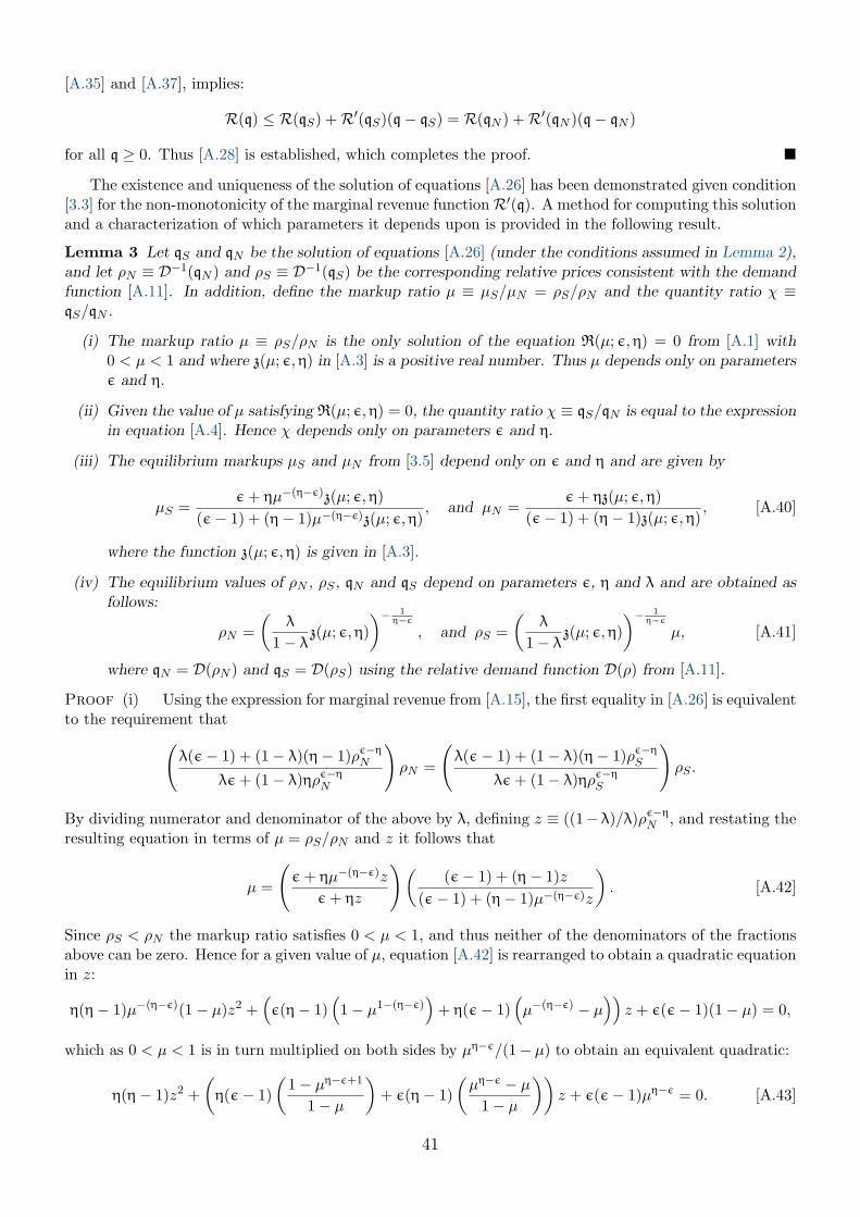
[A.35] and [A.37], implies:
R(q) ≤ R(qS) +R′(qS)(q− qS) = R(qN ) +R′(qN )(q− qN )
for all q ≥ 0. Thus [A.28] is established, which completes the proof.
The existence and uniqueness of the solution of equations [A.26] has been demonstrated given condition[3.3] for the non-monotonicity of the marginal revenue functionR′(q). A method for computing this solutionand a characterization of which parameters it depends upon is provided in the following result.
Lemma 3 Let qS and qN be the solution of equations [A.26] (under the conditions assumed in Lemma 2),and let ρN ≡ D−1(qN ) and ρS ≡ D−1(qS) be the corresponding relative prices consistent with the demandfunction [A.11]. In addition, define the markup ratio µ ≡ µS/µN = ρS/ρN and the quantity ratio χ ≡qS/qN .
(i) The markup ratio µ ≡ ρS/ρN is the only solution of the equation R(µ; ε,η) = 0 from [A.1] with0 < µ < 1 and where z(µ; ε,η) in [A.3] is a positive real number. Thus µ depends only on parametersε and η.
(ii) Given the value of µ satisfying R(µ; ε,η) = 0, the quantity ratio χ ≡ qS/qN is equal to the expressionin equation [A.4]. Hence χ depends only on parameters ε and η.
(iii) The equilibrium markups µS and µN from [3.5] depend only on ε and η and are given by
µS =ε+ ηµ−(η−ε)z(µ; ε,η)
(ε− 1) + (η− 1)µ−(η−ε)z(µ; ε,η), and µN =
ε+ ηz(µ; ε,η)(ε− 1) + (η− 1)z(µ; ε,η)
, [A.40]
where the function z(µ; ε,η) is given in [A.3].
(iv) The equilibrium values of ρN , ρS , qN and qS depend on parameters ε, η and λ and are obtained asfollows:
ρN =(
λ
1− λz(µ; ε,η))− 1
η−ε
, and ρS =(
λ
1− λz(µ; ε,η))− 1
η−ε
µ, [A.41]
where qN = D(ρN ) and qS = D(ρS) using the relative demand function D(ρ) from [A.11].
Proof (i) Using the expression for marginal revenue from [A.15], the first equality in [A.26] is equivalentto the requirement that(
λ(ε− 1) + (1− λ)(η− 1)ρε−ηN
λε+ (1− λ)ηρε−ηN
)ρN =
(λ(ε− 1) + (1− λ)(η− 1)ρε−ηS
λε+ (1− λ)ηρε−ηS
)ρS .
By dividing numerator and denominator of the above by λ, defining z ≡ ((1− λ)/λ)ρε−ηN , and restating theresulting equation in terms of µ = ρS/ρN and z it follows that
µ =
(ε+ ηµ−(η−ε)z
ε+ ηz
)((ε− 1) + (η− 1)z
(ε− 1) + (η− 1)µ−(η−ε)z
). [A.42]
Since ρS < ρN the markup ratio satisfies 0 < µ < 1, and thus neither of the denominators of the fractionsabove can be zero. Hence for a given value of µ, equation [A.42] is rearranged to obtain a quadratic equationin z:
η(η− 1)µ−(η−ε)(1− µ)z2 +(ε(η− 1)
(1− µ1−(η−ε)
)+ η(ε− 1)
(µ−(η−ε) − µ
))z + ε(ε− 1)(1− µ) = 0,
which as 0 < µ < 1 is in turn multiplied on both sides by µη−ε/(1− µ) to obtain an equivalent quadratic:
η(η− 1)z2 +(η(ε− 1)
(1− µη−ε+1
1− µ
)+ ε(η− 1)
(µη−ε − µ
1− µ
))z + ε(ε− 1)µη−ε = 0. [A.43]
41

This quadratic is denoted by Q(z;µ, ε,η) ≡ a0(µ; ε,η)+a1(µ; ε,η)z+a2(η)z2, where the coefficient functionsa0(µ; ε,η), a1(µ; ε,η) and a2(η) listed in [A.2] are obtained directly from [A.43].
Now note that R(qN ) − qNR′(qN ) = R(qS) − qSR′(qS) is deduced by rearranging the equations in[A.26]. The definition of the revenue function R(q) in [A.14] shows that R (D(ρ)) = ρD(ρ) is a validalternative expression for all ρ > 0. By combining these two observations and substituting qS = D(ρS) andqN = D(ρN ), the relative prices and quantities must satisfy
qS(ρS −R′(qS)
)= qN
(ρN −R′(qN )
). [A.44]
After expressing this in terms of the quantity ratio χ ≡ qS/qN and dividing both sides by R′(qS) = R′(qN )(justified by [A.26]), equation [A.44] becomes
χ =(
ρNR′ (D(ρN ))
− 1)/( ρS
R′ (D(ρS))− 1). [A.45]
The formula for marginal revenue R′(D(ρ)) in [A.15] is then rearranged to show
ρ
R′ (D(ρ))− 1 =
λ+ (1− λ)ρε−η
λ(ε− 1) + (η− 1)(1− λ)ρε−η,
which is substituted into [A.45] to obtain
χ =
(λ+ (1− λ)ρε−ηN
λ+ (1− λ)ρε−ηS
)((ε− 1)λ+ (η− 1)(1− λ)ρε−ηS
(ε− 1)λ+ (η− 1)(1− λ)ρε−ηN
).
By dividing numerator and denominator of both fractions by λ and recalling µ = ρS/ρN and the definitionz ≡ ((1− λ)/λ)ρε−ηN , this equation is equivalent to
χ =(
1 + z
1 + µ−(η−ε)z
)((ε− 1) + (η− 1)µ−(η−ε)z
(ε− 1) + (η− 1)z
). [A.46]
The quantity ratio is then written as χ = D(ρS)/D(ρN ) using the relative demand function q = R(ρ)from equation [A.11], and thus
χ =λρ−εS + (1− λ)ρ−ηSλρ−εN + (1− λ)ρ−ηN
.
By factorizing λρ−εS and λρ−εN from the numerator and denominator respectively, and using µ = ρS/ρN andthe definition z ≡ ((1− λ)/λ)ρε−ηN , the above expression for χ becomes
χ = µ−ε(
1 + µ−(η−ε)z1 + z
). [A.47]
Putting together the two expressions for the quantity ratio χ in [A.46] and [A.47], µ and z must satisfythe equation (
1 + z
1 + µ−(η−ε)z
)((ε− 1) + (η− 1)µ−(η−ε)z
(ε− 1) + (η− 1)z
)= µ−ε
(1 + µ−(η−ε)z
1 + z
). [A.48]
Since the quantity ratio χ is finite, none of the terms in the denominators of [A.46] or [A.47] can be zero,
42

so [A.48] is rearranged as follows to obtain a cubic equation in z for a given value of µ:
(η− 1)µ−(2η−ε) (1− µη) z3 + µ−(2η−ε) ((ε− 1)(1− µ2η−ε)+ 2(η− 1) +
(µη−ε − µη
))z2
+ µ−(2η−ε)(
(η− 1)(µ2(η−ε) − µη
)+ 2(ε− 1)
(µη−ε − µ2η−ε)) z
+ (ε− 1)µ−(2η−ε)(µ2(η−ε) − µ2η−ε
)= 0.
Because 0 < µ < 1, both sides of the above are multiplied by µ2η−ε/(1− µη) to obtain an equivalent cubicequation:
(η− 1)z3 +(
(ε− 1)(
1− µ2η−ε
1− µη)
+ 2(η− 1)(µη−ε − µη
1− µη))
z2
+
((η− 1)
(µ2(η−ε) − µη
1− µη
)+ 2(ε− 1)
(µη−ε − µ2η−ε
1− µη))
z
+ (ε− 1)
(µ2(η−ε) − µ2η−ε
1− µη
)= 0. [A.49]
This cubic is denoted by C(z;µ, ε,η) ≡ b0(µ; ε,η)+b1(µ; ε,η)z+b2(µ; ε,η)z2+b3(η)z3, where the coefficientfunctions b0(µ; ε,η), b1(µ; ε,η), b2(µ; ε,η) and b3(η) listed in [A.2] are obtained directly from [A.49].
These steps demonstrate that starting from a solution qS and qN of [A.26], the quadratic and the cubicequations [A.43] and [A.49] in z must simultaneously hold for z = ((1 − λ)/λ)ρε−ηN , with ρN ≡ D−1(qN ),and where the coefficient functions [A.2] are evaluated at µ = ρS/ρN , with ρS ≡ D−1(qS). If the quadraticequation Q(z;µ, ε,η) = 0 and cubic equation C(z;µ, ε,η) = 0 share a root then it is a standard result fromthe theory of polynomials that the resultant R(µ; ε,η), as defined in [A.1], is zero. Since the coefficients ofthe polynomials Q(z;µ, ε,η) and C(z;µ, ε,η) are functions only of the markup ratio µ and the parameters εand η, solving the equation R(µ; ε,η) = 0 provides a straightforward procedure for finding the equilibriummarkup ratio µ. Furthermore, the only parameters appearing in the equation R(µ; ε,η) = 0 are ε and η,so the equilibrium markup ratio µ depends only on these parameters.
Lemma 2 shows that the solution of [A.26] for qS and qN is unique, and therefore the solution ofR(µ; ε,η) = 0 for µ must also be unique, given the added condition that the shared root z of the quadraticQ(z;µ, ε,η) = 0 and cubic C(z;µ, ε,η) = 0 is a positive real number. This restriction is required becausez = ((1− λ)/λ)ρε−ηN and ρN must of course be positive real numbers. Since η > ε > 1, the product of theroots of the quadratic Q(z;µ, ε,η) = 0 is positive, so the shared root z is positive and real if and only ifeither branch of the quadratic root function is positive and real. Hence this condition is verified by checkingwhether z(µ; ε,η) in [A.3] (the smaller of the two roots of Q(z;µ, ε,η) = 0) is positive and real.
Note that the resultant R(µ; ε,η) is always zero at µ = 0 and µ = 1 for all values of ε and η. This isseen by taking limits of the coefficients in [A.2] as µ→ 0 and µ→ 1 and applying L’Hopital’s rule, whichyields
C(z; 0, ε,η) = zQ(z; 0, ε,η), and C(z; 1, ε,η) = (1 + z)Q(z; 1, ε,η).
As the polynomials Q(z;µ, ε,η) and C(z;µ, ε,η) clearly share roots when µ = 0 or µ = 1, it follows thatR(0; ε,η) = R(1; ε,η) = 0. Thus these zeros of the equation R(µ; ε,η) = 0 must be ignored when solvingfor µ.
(ii) The quadratic equation Q(z;µ, ε,η) = 0 with z = ((1 − λ)/λ)ρε−ηN determines a relative price ρNsuch that with ρS = µρN , marginal revenue is equalized at both ρS and ρN . Lemma 1 demonstrates thatthere are two candidate solutions for ρN that meet this criterion under the conditions shown by Lemma 2to be necessary for a solution qS and qN of [A.26] to exist. However, Lemma 2 shows that both ρN andρS are on the downward-sloping sections of the marginal revenue function. To rule out a solution in themiddle upward-sloping section of marginal revenue, the smaller of the two ρN candidate values must bediscarded to select the correct solution. Since z is decreasing in ρN , this is equivalent to discarding thelarger of the two roots of the quadratic. Given that a2(η) in [A.2] is positive, the smaller of the two roots
43

of quadratic Q(z;µ, ε,η) = 0 is found using the expression for z(µ; ε,η) in [A.3].The equilibrium quantity ratio χ is obtained by substituting z = z(µ; ε,η) into [A.47]. This construction
demonstrates that χ depends only on ε and η.
(iii) Since ρS ≡ PS/PB and ρN ≡ PN/PB according to [A.12], the formula for the purchase multipliersin [2.10] implies vN = ρε−ηN and vS = µε−ηvN . Using the fact that z ≡ ((1 − λ)/λ)ρε−ηN , and dividingnumerator and denominator of the expression in [3.4] by λ yields [A.40].
(iv) The expressions for the relative prices ρS and ρN in [A.41] are obtained by rearranging the definitionof z ≡ ((1− λ)/λ)ρε−ηN and using ρS = µρN . This completes the proof.
A.3 Proof of Theorem 1
Non-monotonicity of the marginal revenue function
Using the relationship between the revenue function R(q;PB, E) and its equivalent R(q) defined in [A.14]using the relative demand function D(ρ) from [A.11], the corresponding two marginal revenue functionsR′(q;PB, E) and R′(q) are proportional according to [A.17]. Lemma 1 demonstrates that R′(q) has thedescribed pattern of non-monotonicity under the conditions 0 < λ < 1 and [3.3], and is otherwise adecreasing function of q.
Existence of a two-price equilibrium
For a two-price equilibrium to exist, first-order conditions [3.2] for profit-maximization must be satisfiedat two prices pS and pN , with associated quantities qS = D(pS ;PB, E) and qN = D(pN ;PB, E), where PBis the bargain hunters’ price index from [2.7], and E = P εY is the measure of aggregate expenditure from[2.10].
The necessary conditions for the two-price equilibrium are now restated in terms of the relative demandfunction D(ρ) defined in [A.11], and its associated total and marginal revenue functions R(q) and R′(q),as defined in [A.14] and analysed in appendix A.2. The relative demand function q = D(ρ) is specified interms of the relative price ρ ≡ p/PB and relative quantity q ≡ q/(E/P εB), in accordance with [A.12]. Usingthe relationships in [A.13] and [A.17], the first two optimality conditions in [3.2] are equivalent to
R′(qSP
εB
E
)= R′
(qNP
εB
E
)=R(qSP
εBE
)−R
(qNP
εBE
)qSP
εBE − qNP
εBE
. [A.50]
With qS ≡ qS/(E/P εB) and qN ≡ qN/(E/P εB), the first-order conditions in [A.50] are identical to theequations in [A.26] studied in Lemma 2. These clearly require the equalization of marginal revenue R′(q) attwo different quantities, which means that the marginal revenue function must be non-monotonic. Lemma 1then shows that 0 < λ < 1 and parameters ε and η satisfying the inequality [3.3] are necessary and sufficientfor this. If these conditions are met then Lemma 2 demonstrates the existence of a unique solution qS andqN of the equations [A.26].
The relative quantities qS and qN must also be well defined if the solution is to be economicallymeaningful. This means that if ρS = D−1(qS) and ρN = D−1(qN ) are the corresponding prices pS andpN relative to PB then ρS < 1 < ρN . This is a necessary requirement because the expression [3.7] for thebargain hunters’ price index PB implies
sρ1−ηS + (1− s)ρ1−η
N = 1, [A.51]
and the equilibrium sales frequency s must satisfy s ∈ (0, 1).Assume the parameters are such that ε and η satisfy [3.3], and consider a given value of λ ∈ (0, 1).
Lemma 3 shows that the markup ratio (or price ratio) µ ≡ µS/µN = ρS/ρN consistent with the uniquesolution of [A.26] is a function only of the elasticities ε and η. The equilibrium relative prices ρS and ρN
44

are functions of all three parameters ε, η and λ, and are obtained from equation [A.41] by substitutingthe equilibrium value of µ into the function z(µ; ε,η) defined in [A.3]. Since ρS = µρN and µ < 1, therequirement ρS < 1 < ρN implies µ < ρS < 1. By substituting for ρS from [A.41], this condition isequivalent to:
z (µ; ε,η) <1− λλ
< µ−(η−ε)z (µ; ε,η) . [A.52]
Define lower and upper bounds for λ conditional on ε and η using the formulæ in [A.6] together with theequilibrium value of µ (which is a function only of ε and η) and the function z(µ; ε,η) from [A.3]. Notethat if z(µ; ε,η) > 0 and 0 < µ < 1 then 0 < λ(ε,η) < λ(ε,η) < 1. By rearranging the inequality [A.52]and using the definitions of the bounds on λ, the inequality is equivalent to λ lying in the interval:
λ(ε,η) < λ < λ(ε,η). [A.53]
This restriction on λ is necessary and sufficient for the existence of an equilibrium sales frequency s ∈ (0, 1)satisfying [A.51]. The equivalence is demonstrated by substituting the expressions for ρS and ρN from[A.41] into [A.51]: (
1 + s(µ−(η−1) − 1
))( λ
1− λz(µ; ε,η)) η−1
η−ε
= 1.
This is a linear equation in s, and has a unique solution because η > 1 and 0 < µ < 1. Solving explicitlyfor s yields:
s =
(λ
1−λz(µ; ε,η))−( η−1
η−ε
)− 1
µ−(η−1) − 1. [A.54]
Recalling the equivalence of inequalities [A.52] and [A.53], it follows that s ∈ (0, 1) if and only if λ ∈(λ(ε,η), λ(ε,η)). So for λ ∈ [0, λ(ε,η)] or λ ∈ [λ(ε,η), 1] there is no two-price equilibrium. But givenelasticities ε and η satisfying the non-monotonicity condition [3.3] and a loyal fraction λ ∈ (λ(ε,η), λ(ε,η)),by using the arguments above there exist two distinct relative prices ρS ≡ pS/PB and ρN ≡ pN/PB and asales frequency s ∈ (0, 1) consistent with the first two equalities in [3.2]. Lemma 3 then demonstrates thatthe two purchase multipliers vS and vN and the two optimal markups µS and µN are determined. Equations[3.1] and [3.4] show that using the optimal markups in [3.5] is equivalent to satisfying the remainingfirst-order condition involving marginal cost in [3.2]. The other variables relevant to the macroeconomicequilibrium are then determined as discussed in section 3.4.
Confirming that the two-price equilibrium exists then requires checking that the remaining first-ordercondition [2.13c] is satisfied and that the first-order conditions are sufficient as well as necessary to charac-terize the maximum of the profit function. Using the relationships in [A.17] and the results of Lemma 2 in[A.27] the following inequalities are deduced:
R(qS ;PB, E)−R′(qS ;PB, E)qS > 0, and R(qN ;PB, E)−R′(qN ;PB, E)qN > 0. [A.55]
Since s ∈ (0, 1), the Lagrangian multiplier ℵ from first-order conditions [2.13b]–[2.13c] is determined asfollows:
ℵ = R(qS ;PB, E)−R′(qS ;PB, E)qS = R(qN ;PB, E)−R′(qN ;PB, E)qN ,
and hence ℵ > 0 because of [A.55]. By combining this expression for the Lagrangian multiplier with thefirst-order condition [2.13c]:
R(q;PB, E) ≤ R(qN ;PB, E) + R′(qN ;PB, E)(q − qN ) = R(qS ;PB, E) + R′(qS ;PB, E)(q − qS), [A.56]
which is required to hold for all q ≥ 0. Appealing to the result of Lemma 2 in [A.28] and again using [A.17]verifies the inequality.
The assumptions about the production function [2.8] ensure that the total cost function C (Q;W ) in
45

[2.9] is continuously differentiable and convex, so for all q ≥ 0:
C (q;W ) ≥ C (Q;W ) + C ′(Q;W )(q −Q), [A.57]
where Q ≡ sqS+(1−s)qN is the specific total physical quantity sold using the two-price strategy constructedearlier. Now consider a general alternative pricing strategy for a given firm, assuming that all other firmscontinue to use the same two-price strategy. The new strategy is specified in terms of a distribution functionF (p) for prices. Let G(q) ≡ 1 − F (D(p;PB, E)) be the implied distribution function for quantities sold.The level of profits P from the new strategy is obtained by making a change of variable from prices toquantities in the integrals of [2.12]:
P =∫qR(q;PB, E)dG(q)− C
(∫qqdG(q);W
).
Applying the inequalities involving the revenue and total cost functions from [A.56] and [A.57] to theexpression for profits yields:
P ≤(R(qN ;PB, E)−R′(qN ;PB, E)qN
)−(C (Q;W )− C ′(Q;W )Q
)+(R′(qN ;PB, E)− C ′(Q;W )
)(∫qqdG(q)
).
The first-order conditions [3.2] imply that the coefficient of the integral in the above expression is zero, andthat R(qN ;PB, E)−R′(qN ;PB, E)qN = R(qS ;PB, E)−R′(qS ;PB, E)qS . Recalling Q = sqS + (1− s)qN , itfollows that:
P ≤ sR(qS ;PB, E) + (1− s)R(qN ;PB, E)− C (sqS + (1− s)qN ;W ) ,
for all alternative pricing strategies. Hence there is no profit-improving deviation from the two-pricestrategy. This establishes that a two-price equilibrium exists when [3.3] and λ ∈ (λ(ε,η), λ(ε,η)) hold, andthat it is unique within the class of two-price equilibria.
Uniqueness of the two-price equilibrium
Suppose the parameters ε, η and λ are such that a two-price equilibrium exists. Now consider the possibilitythat a one-price equilibrium also exists for the same parameters. Since all firms are symmetric, the relativeprice found in this one-price equilibrium is necessarily equal to one. The relative prices ρS and ρN in thetwo-price equilibrium cannot be on the same side of one, implying µ < ρS < 1 and thus ρS < 1 < ρN , whereρS = D−1(qS) and ρN = D−1(qN ) using the relative quantities qS and qN . Since [A.11] implies D(1) = 1and because the relative demand function D(ρ) is strictly decreasing in ρ, it follows that qN < 1 < qS .
Given that the marginal revenue function must be non-monotonic if a two-price equilibrium is to exist,it follows from Lemma 1 that R(q) is strictly concave on the intervals (0, q) and (q,∞), strictly convex on(q, q), and from Lemma 2 that qN < q < q < qS .
Consider first the case where q < 1 < q. Since q1 = 1 for all firms in the one-price equilibrium, theactual common quantity produced is q1 = E/P εB using [A.12], where PB and E are the values of thesevariables associated with the putative one-price equilibrium. Since R′′(1) > 0, equation [A.17] impliesR′′(q1;PB, E) > 0. Therefore, for sufficiently small ε > 0, the profits P from selling quantity q1 − ε at onehalf of shopping moments and q1 + ε at the other half exceed the profits from offering one price and henceone quantity at all shopping moments:
12R(q1 − ε;PB, E) +
12R(q1 + ε;PB, E)− C
(12
(q1 − ε) +12
(q1 + ε);W)> R(q1;PB, E)− C (q1;W ).
Therefore a one-price equilibrium cannot exist in this case.Next consider the case where qN < 1 < q. Let p1 = PB denote the price it is claimed all firms charge
in a one-price equilibrium, and q1 = E/P εB the associated quantity sold. Now let qS = D(ρSp1;PB, E) bequantity sold if the sale relative price ρS = D−1(qS) is used when other firms are following the one-price
46
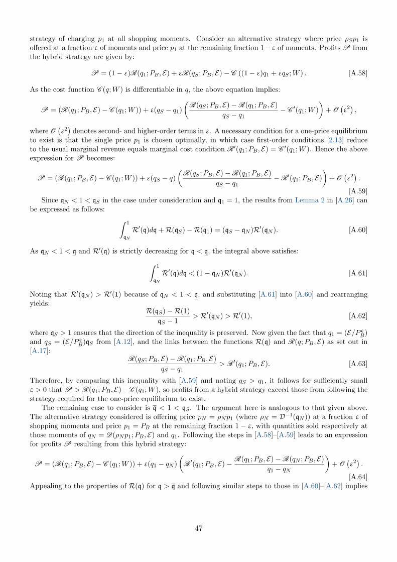
strategy of charging p1 at all shopping moments. Consider an alternative strategy where price ρSp1 isoffered at a fraction ε of moments and price p1 at the remaining fraction 1− ε of moments. Profits P fromthe hybrid strategy are given by:
P = (1− ε)R(q1;PB, E) + εR(qS ;PB, E)− C ((1− ε)q1 + εqS ;W ) . [A.58]
As the cost function C (q;W ) is differentiable in q, the above equation implies:
P = (R(q1;PB, E)− C (q1;W )) + ε(qS − q1)(
R(qS ;PB, E)−R(q1;PB, E)qS − q1
− C ′(q1;W ))
+ O(ε2),
where O(ε2)
denotes second- and higher-order terms in ε. A necessary condition for a one-price equilibriumto exist is that the single price p1 is chosen optimally, in which case first-order conditions [2.13] reduceto the usual marginal revenue equals marginal cost condition R′(q1;PB, E) = C ′(q1;W ). Hence the aboveexpression for P becomes:
P = (R(q1;PB, E)− C (q1;W )) + ε(qS − q)(
R(qS ;PB, E)−R(q1;PB, E)qS − q1
−R′(q1;PB, E))
+ O(ε2).
[A.59]Since qN < 1 < qS in the case under consideration and q1 = 1, the results from Lemma 2 in [A.26] can
be expressed as follows: ∫ 1
qN
R′(q)dq +R(qS)−R(q1) = (qS − qN )R′(qN ). [A.60]
As qN < 1 < q and R′(q) is strictly decreasing for q < q, the integral above satisfies:∫ 1
qN
R′(q)dq < (1− qN )R′(qN ). [A.61]
Noting that R′(qN ) > R′(1) because of qN < 1 < q, and substituting [A.61] into [A.60] and rearrangingyields:
R(qS)−R(1)qS − 1
> R′(qN ) > R′(1), [A.62]
where qS > 1 ensures that the direction of the inequality is preserved. Now given the fact that q1 = (E/P εB)and qS = (E/P εB)qS from [A.12], and the links between the functions R(q) and R(q;PB, E) as set out in[A.17]:
R(qS ;PB, E)−R(q1;PB, E)qS − q1
> R′(q1;PB, E). [A.63]
Therefore, by comparing this inequality with [A.59] and noting qS > q1, it follows for sufficiently smallε > 0 that P > R(q1;PB, E)−C (q1;W ), so profits from a hybrid strategy exceed those from following thestrategy required for the one-price equilibrium to exist.
The remaining case to consider is q < 1 < qS . The argument here is analogous to that given above.The alternative strategy considered is offering price pN = ρNp1 (where ρN = D−1(qN )) at a fraction ε ofshopping moments and price p1 = PB at the remaining fraction 1− ε, with quantities sold respectively atthose moments of qN = D(ρNp1;PB, E) and q1. Following the steps in [A.58]–[A.59] leads to an expressionfor profits P resulting from this hybrid strategy:
P = (R(q1;PB, E)− C (q1;W )) + ε(q1 − qN )(
R′(q1;PB, E)− R(q1;PB, E)−R(qN ;PB, E)q1 − qN
)+ O
(ε2).
[A.64]Appealing to the properties of R(q) for q > q and following similar steps to those in [A.60]–[A.62] implies
47

R′(1) > R′(qS) > (R(1)−R(qN ))/(1− qN ), and hence an equivalent of [A.63]:
R′(q1;PB, E) >R(q1;PB, E)−R(qN ;PB, E)
q1 − qN. [A.65]
Since q1 > qN , for sufficiently small ε > 0, [A.64] and [A.65] demonstrate that there is a hybrid strategywhich delivers higher profits than the one-price strategy used by all other firms. This proves that for allparameters where the two-price equilibrium exists, a one-price equilibrium cannot exist for any of thesesame parameter values.
One-price equilibrium
The first point to note is that when a two-price equilibrium fails to exist owing to a violation of the non-monotonicity condition [3.3], Lemma 1 implies that marginal revenue R′(q;PB, E) is strictly decreasing forall q. This is equivalent to revenue R(q;PB, E) being a strictly concave function of quantity q. Since totalcost C (q;W ) is a convex function of the quantity produced, it follows immediately that the profit functionis globally concave, and thus a one-price equilibrium always exists, and is the only possible equilibrium inthe parameter range where ε or η fail to satisfy [3.3], or where λ = 0 or λ = 1.
Now suppose the parameters are such that the marginal revenue function is non-monotonic, but a two-price equilibrium fails to exist owing to λ not lying between λ(ε,η) and λ(ε,η). Note that [A.52] and [A.6]imply λ ∈ [0, λ(ε,η)] and λ ∈ [λ(ε,η), 1] are equivalent to 1 > qS and 1 < qN respectively.
Taking the first of these cases, Lemma 1 demonstrates the concavity of R(q) on [q,∞) (containing qS),which establishes that R(q) ≤ R(1) +R′(1)(q− 1) for all q ∈ [q,∞). Lemma 2 shows that R(q) ≤ R(qS) +R′(qS)(q− qS) for all q ≥ 0. Note that the concavity of R(q) in the relevant range implies R′(qS) > R′(1),which together with the second of the previous inequalities yields R(q) ≤ R(qS) + R′(1)(q − qS) for allq ∈ [0, qS ]. Applying the first inequality at q = qS establishes that R(qS) ≤ R(1) + R′(1)(qS − 1). Bycombining these results it follows that R(q) ≤ R(1) +R′(1)(q − 1) for all q ≥ 0. Translating this into aproperty of the original revenue function R(q;PB, E) using [A.12] and [A.17] yields the following for all q:
R(q;PB, E) ≤ R(q1;PB, E) + R′(q1;PB, E)(q − q1). [A.66]
When λ ∈ [λ(ε,η), 1] the other case to consider is 1 < qN . Using an exactly analogous argument tothat given above, it is deduced that R(q) ≤ R(1) +R′(1)(q − 1) for all q ≥ 0 in this case as well. Hence[A.66] holds in both cases. The convexity of the total cost function C (q;W ) together with [A.66] provesthat no pricing strategy can improve on that used in the one-price equilibrium.
Non-existence of equilibria with more than two prices
Take any two prices p1 and p2 offered by a firm at a positive fraction of shopping moments, and defineρ1 ≡ p1/PB and ρ2 ≡ p2/PB in accordance with [A.12]. Denote the quantities sold by q1 and q2 and defineq1 ≡ (P εB/E)q1 and q2 ≡ (P εB/E)q2 also in accordance with [A.12]. Using the first-order conditions [2.13]together with [A.12] and [A.17], it follows that q1 and q2 must satisfy the system of equations [A.26] inplace of qS and qN . But as Lemma 2 demonstrates that the solution to this system of equations is unique,there is a maximum of two distinct prices in any firm’s profit-maximizing strategy. This completes theproof.
A.4 Proof of Proposition 1
(i) The first-order conditions are of course necessary. For sufficiency, note using the argument in theproof of Theorem 1 that the first-order conditions in [3.2] are equivalent to the equations in [A.50]. AsLemma 3 shows, the equations in [A.50] have a unique solution. Since an equilibrium is known to exist byTheorem 1, the first-order conditions must also be sufficient.
(ii) Lemma 3 shows that µ, χ, µS and µN are uniquely determined as functions of ε and η when theinequality [3.3] is satisfied, as is necessary for the two-price equilibrium to exist.
48

(iii) Lemma 3 implicitly determines the purchase multipliers vS and vN using the expressions for ρS ≡pS/PB and ρN = pN/PB in [A.41] and the fact that vS = (pS/PB)−(η−ε) and vN = (pN/PB)−(η−ε) from[2.10]. Hence Lemma 3 shows that these variables depend only on ε, η and λ. In conjunction with equation[3.7], knowledge of ρS and ρN from [A.41] yields a linear equation for s after dividing both sides of [3.7] byPB. This shows that it too only depends on ε, η and λ.
(iv) Substituting the bounds for λ from [A.6] into equation [A.54] proves the first two results. Differen-tiating [A.54] with respect to λ yields the third result. This completes the proof.
A.5 Proof of Theorem 2
Log linearizations
The notational convention adopted here is that a variable without a time subscript denotes its flexible-price steady-state value as determined in section 3, and the corresponding sans serif letter denotes the logdeviation of the variable from its steady-state value (except for the sales frequency s, where it denotes justthe deviation from steady state, and the inflation rate, where it denotes the log deviation of the gross rate).
Consider first the demand function faced by firms. The levels of demand qS,`,t and qN,`,t at the sale andnormal prices are obtained from [3.9], which have the following log-linearized forms:
qS,`,t =(
(1− λ)vSλ+ (1− λ)vS
)vS,`,t − ε(pS,`,t − Pt) + Yt, and [A.67a]
qN,`,t =(
(1− λ)vNλ+ (1− λ)vN
)vN,`,t − ε(RN,t−` − Pt) + Yt, [A.67b]
where the expressions are given in terms of log deviations of the purchase multipliers vS,`,t and vN,`,t from[2.10]:
vS,`,t = −(η− ε) (pS,`,t − PB,t) , and vN,`,t = −(η− ε) (RN,t−` − PB,t) . [A.68]
By substituting the purchase multipliers into the demand functions [A.67], the following expressions arefound:
qS,`,t = −(λε+ (1− λ)ηvSλ+ (1− λ)vS
)pS,`,t + (η− ε)
((1− λ)vS
λ+ (1− λ)vS
)PB,t + εPt + Yt, and [A.69a]
qN,`,t = −(λε+ (1− λ)ηvNλ+ (1− λ)vN
)RN,t−` + (η− ε)
((1− λ)vN
λ+ (1− λ)vN
)PB,t + εPt + Yt. [A.69b]
From equation [3.4], the log-linearized optimal markups at given sale and normal prices are:
µS,`,t = −cSvS,`,t, with cS ≡λ(1− λ)(η− ε)vS
(λε+ (1− λ)ηvS) (λ(ε− 1) + (1− λ)(η− 1)vS), and [A.70a]
µN,`,t = −cNvN,`,t, with cN ≡λ(1− λ)(η− ε)vN
(λε+ (1− λ)ηvN ) (λ(ε− 1) + (1− λ)(η− 1)vN ), [A.70b]
which are given in terms of the purchase multipliers from [A.68]. Overall demand Q`,t = s`,tqS,`,t + (1 −s`,t)qN,`,t is log-linearized as follows:
Q`,t =(
χ− 1sχ+ (1− s)
)s`,t +
(sχ
sχ+ (1− s)
)qS,`,t +
(1− s
sχ+ (1− s)
)qN,`,t. [A.71]
Define the following weighted averages of variables across the distribution of normal-price vintages.First, the average sale frequency:
st ≡ (1− φp)∞∑`=0
φ`ps`,t.
49
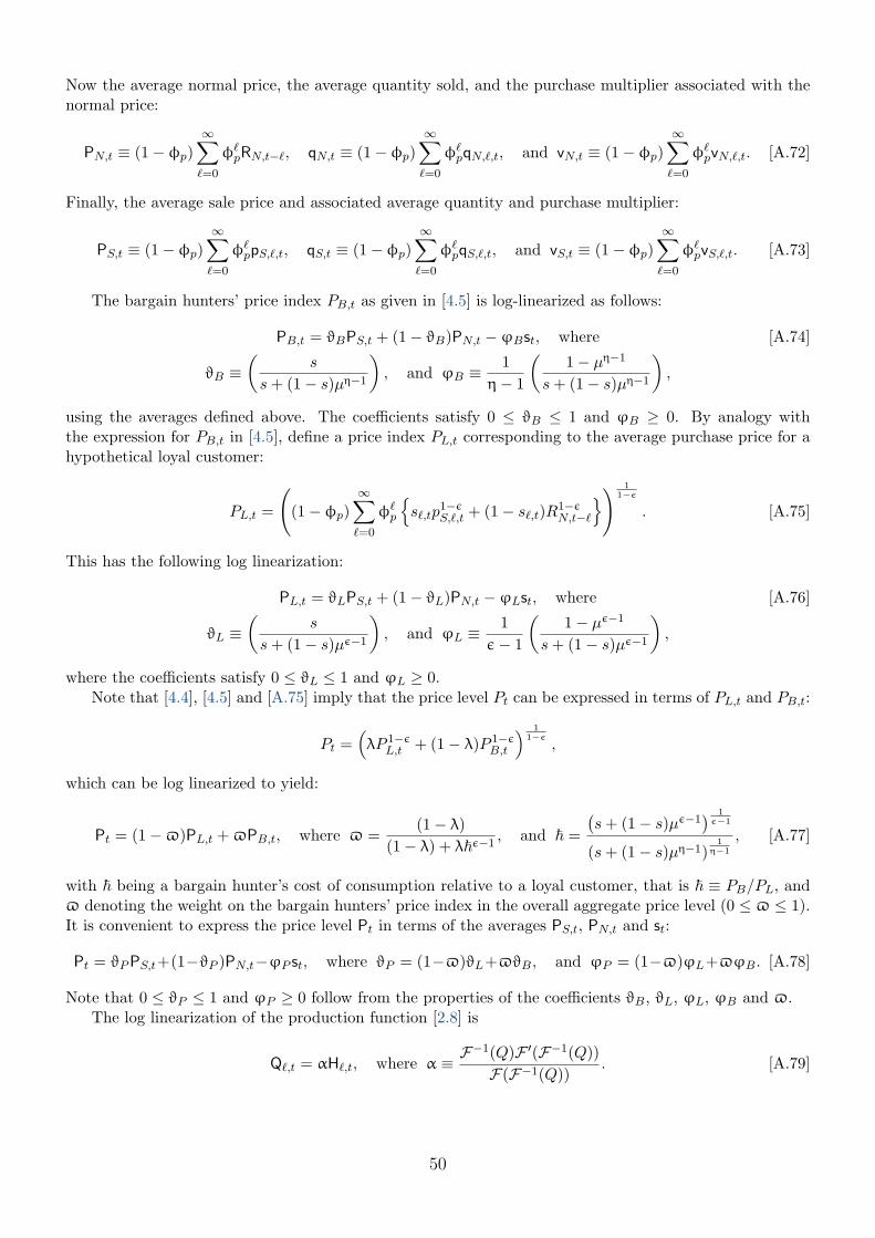
Now the average normal price, the average quantity sold, and the purchase multiplier associated with thenormal price:
PN,t ≡ (1− φp)∞∑`=0
φ`pRN,t−`, qN,t ≡ (1− φp)∞∑`=0
φ`pqN,`,t, and vN,t ≡ (1− φp)∞∑`=0
φ`pvN,`,t. [A.72]
Finally, the average sale price and associated average quantity and purchase multiplier:
PS,t ≡ (1− φp)∞∑`=0
φ`ppS,`,t, qS,t ≡ (1− φp)∞∑`=0
φ`pqS,`,t, and vS,t ≡ (1− φp)∞∑`=0
φ`pvS,`,t. [A.73]
The bargain hunters’ price index PB,t as given in [4.5] is log-linearized as follows:
PB,t = ϑBPS,t + (1− ϑB)PN,t −ϕBst, where [A.74]
ϑB ≡(
s
s+ (1− s)µη−1
), and ϕB ≡
1η− 1
(1− µη−1
s+ (1− s)µη−1
),
using the averages defined above. The coefficients satisfy 0 ≤ ϑB ≤ 1 and ϕB ≥ 0. By analogy withthe expression for PB,t in [4.5], define a price index PL,t corresponding to the average purchase price for ahypothetical loyal customer:
PL,t =
((1− φp)
∞∑`=0
φ`p
s`,tp
1−εS,`,t + (1− s`,t)R1−ε
N,t−`
) 11−ε
. [A.75]
This has the following log linearization:
PL,t = ϑLPS,t + (1− ϑL)PN,t −ϕLst, where [A.76]
ϑL ≡(
s
s+ (1− s)µε−1
), and ϕL ≡
1ε− 1
(1− µε−1
s+ (1− s)µε−1
),
where the coefficients satisfy 0 ≤ ϑL ≤ 1 and ϕL ≥ 0.Note that [4.4], [4.5] and [A.75] imply that the price level Pt can be expressed in terms of PL,t and PB,t:
Pt =(λP 1−ε
L,t + (1− λ)P 1−εB,t
) 11−ε
,
which can be log linearized to yield:
Pt = (1−$)PL,t +$PB,t, where $ =(1− λ)
(1− λ) + λ~ε−1, and ~ =
(s+ (1− s)µε−1
) 1ε−1
(s+ (1− s)µη−1)1
η−1
, [A.77]
with ~ being a bargain hunter’s cost of consumption relative to a loyal customer, that is ~ ≡ PB/PL, and$ denoting the weight on the bargain hunters’ price index in the overall aggregate price level (0 ≤ $ ≤ 1).It is convenient to express the price level Pt in terms of the averages PS,t, PN,t and st:
Pt = ϑPPS,t+(1−ϑP )PN,t−ϕP st, where ϑP = (1−$)ϑL+$ϑB, and ϕP = (1−$)ϕL+$ϕB. [A.78]
Note that 0 ≤ ϑP ≤ 1 and ϕP ≥ 0 follow from the properties of the coefficients ϑB, ϑL, ϕL, ϕB and $.The log linearization of the production function [2.8] is
Q`,t = αH`,t, where α ≡ F−1(Q)F ′(F−1(Q))F(F−1(Q))
. [A.79]
50
The nominal marginal cost function corresponding to [2.9] has the following log-linear form:
X`,t = γQ`,t+Wt, where γ ≡ QC ′′(Q;W )C ′(Q;W )
=(−F
−1(Q)F ′′(F−1(Q))F ′(F−1(Q))
)(Q
F−1(Q)F ′(F−1(Q))
). [A.80]
(i) The log-linearized first-order condition for the sales frequency (the first equation in [4.3]) is
(χ− 1)X`,t = µSχpS,`,t − µNRN,t−` + (µS − 1)χ(qS,`,t − qN,`,t), [A.81]
where the fact that χ = (µN − 1)/(µS − 1) is used to simplify the expression. By using equation [A.69]:
(χ− 1)X`,t =(µS − (µS − 1)
(λε+ (1− λ)ηvSλ+ (1− λ)vS
))χpS,`,t
−(µN − (µN − 1)
(λε+ (1− λ)ηvNλ+ (1− λ)vN
))RN,t−`
+ (η− ε)(
(1− λ)vSλ+ (1− λ)vS
− (1− λ)vNλ+ (1− λ)vN
)(µS − 1)χPB,t.
Given the expressions for µS and µN in [3.4], the coefficients of both pS,`,t and RN,`,t in the above are zero.Since χ > 1, this equation implies X`,t is independent of pS,`,t and RN,t−`. Using χ = (µN − 1)/(µS − 1)yields:
(χ− 1)X`,t = (χ− 1)PB,t −(
1− (η− ε)(
(1− λ)vSλ+ (1− λ)vS
)(µS − 1)
)χPB,t
+(
1− (η− ε)(
(1− λ)vNλ+ (1− λ)vN
)(µN − 1)
)PB,t. [A.82]
After substituting the expressions for µS and µN from [3.5], the above equation reduces to
(χ− 1)X`,t = (χ− 1)PB,t + (ε− 1) ((µS − 1)χ− (µN − 1)) PB,t,
and noting that the coefficient on the final term is zero, it follows that X`,t = PB,t for all `. Hence, all firmshave the same marginal cost, Xt = PB,t, irrespective of their normal-price vintage.
The optimal pS,`,t is characterized by the second equation in [4.3]. In log-linear terms it is
pS,`,t = µS,`,t + Xt.
By substituting the expressions for the log-linearized optimal sale markup from [A.70] and the sale purchasemultiplier from [A.68], and using Xt = PB,t:
(1− (η− ε)cS) (pS,`,t − Xt) = 0, [A.83]
so pS,`,t = Xt if the coefficient in the above is different from zero. The expressions for cS from [A.70] andµS from [3.5] imply
(1− (η− ε)cS)µS
=(λ(ε− 1) + (1− λ)(η− 1)vS) (λε+ (1− λ)ηvS)− (η− ε)2λ(1− λ)vS
(λε+ (1− λ)ηvS)2 .
Using [A.18] and noting that vS = ρε−ηS it follows that 1 − (η − ε)cS = µSD′(ρS)R′′(D(ρS)), where thefunctions D(ρ) and R(q) are defined in [A.11] and [A.14]. The coefficient in [A.83] is strictly positivebecause D′(ρS) < 0 and Lemma 2 shows that R′′(D(ρS)) < 0, and therefore pS,`,t = Xt.
Since all firms face the same wage Wt, and as the argument above shows that all have the same nominalmarginal cost Xt, the log linearization of nominal marginal cost in [A.80] shows that all must produce thesame total quantity Qt when γ > 0.
51

The log-linearization of the first-order condition [4.2] for the optimal reset price RN,t simplifies to
∞∑`=0
(βφp)`Et [RN,t − µN,`,t+` − Xt+`] = 0, [A.84]
where µN,`,t is the log-deviation of the optimal markup µN,`,t ≡ µ(RN,t−`;PB,t). The optimal markupfunction is log-linearized in [A.70] and is given in terms of the corresponding purchase multiplier, itselflog-linearized in [A.68]. Putting those results together, it follows that µN,`,t+` = (η− ε)cN (RN,t − PB,t+`).So by using Xt = PB,t and substituting these results into [A.84]:
(1− (η− ε)cN )∞∑`=0
(βφp)`Et [RN,t − Xt+`] = 0.
An exactly analogous argument to the proof of 1− (η− ε)cS > 0 above shows that 1− (η− ε)cN > 0 alsoholds. Hence:
RN,t = (1− βφp)∞∑`=0
(βφp)`EtXt+`. [A.85]
(ii) By using PS,t = Xt and substituting this into [A.78] it is demonstrated that
ϕP st = ϑP (Xt − Pt) + (1− ϑP )(PN,t − Pt). [A.86]
Likewise, by using PB,t = Xt and performing similar substitutions in the expression for PB,t from [A.74]:
ϕBst = (1− ϑB)(PN,t − Xt). [A.87]
Equation [A.86] can be written as
ϕP st = ϑP (Xt − Pt) + (1− ϑP ) ((PN,t − Xt) + (Xt − Pt)) ,
and st is eliminated using [A.87]. After some rearrangement this leads to
Xt − PN,t =1
1−ψxt, [A.88]
where xt = Xt − Pt is real marginal cost and ψ is defined as follows:
ψ =(1− ϑB)ϕP + ϑPϕB
ϕB. [A.89]
Note that the recursive form of the expression for PN,t in [A.72] is
PN,t = φpPN,t−1 + (1− φp)RN,t, [A.90]
and the recursive form of the equation [A.85] for RN,t is:
RN,t = βφpEtRt+1 + (1− βφp)Xt. [A.91]
Then multiplying both sides of the above by (1 − φp) and substituting in the recursive equation for PN,tyields
PN,t − φpPN,t−1 = βφpEt [PN,t+1 − φpPN,t] + (1− φp)(1− βφp)Xt,which can be written in terms of normal-price inflation πN,t ≡ PN,t − PN,t−1:
πN,t = βEtπN,t+1 + κ(Xt − PN,t), [A.92]
52

and where κ = (1− φp)(1− βφp)/φp is as defined in the statement of the theorem.Taking the first difference of [A.87] yields
∆st = −(1− ϑB)ϕB
(∆Xt − πN,t) . [A.93]
Now use [A.78] and make the substitution PS,t = Xt as before, and then take first differences and rearrange:
πt = πN,t + ϑP (∆Xt − πN,t)−ϕP∆st.
By eliminating ∆st from this equation using [A.93]:
πt = πN,t +ψ (∆Xt − πN,t) .
Substituting the first difference of equation [A.88] into the above yields
πN,t = πt −ψ
1−ψ∆xt.
Combining this equation with [A.88] and [A.92] implies(πt −
ψ
1−ψ∆xt
)= βEt
[πt+1 −
ψ
1−ψ∆xt+1
]+
κ
1−ψxt,
which is rearranged to yield the result [4.8]. Recursive forward substitution of equation [4.8] leads to
πt =1
1−ψ∞∑`=0
β`Et [κxt+` +ψ (∆xt+` − β∆xt+1+`)] .
Notice that all ∆xt+` terms apart from ∆xt cancel out because each occurs twice with opposite signs.Hence equation [4.9] is obtained.
(iii) Equation [A.89] implies that an expression for 1−ψ is
1−ψ =(1− ϑP )ϕB − (1− ϑB)ϕP
ϕB. [A.94]
It follows from [A.78] that (1− ϑP ) = (1−$)(1− ϑL) +$(1− ϑB). Together with the expression for ϕPfrom the same equation, [A.94] implies
1−ψ =((1−$)(1− ϑL) +$(1− ϑB))ϕB − (1− ϑB) ((1−$)ϕL +$ϕB)
ϕB,
and by rearranging this expression:
1−ψ = (1−$)ϕL
(1− ϑLϕL
− 1− ϑBϕB
). [A.95]
Define the function
Φ(ζ;µ) ≡ µ−ζ − 1ζ
[A.96]
in terms of the markup ratio µ. An alternative expression for this function is Φ(ζ;µ) = (e(− logµ)ζ − 1)/ζ,which shows that it has derivative
Φ′(ζ;µ) =((− logµ)ζ − 1) e(− log µ)ζ + 1
ζ2.
53

Now define another functionJ (z) ≡ 1 + (z − 1)ez,
and note that J ′(z) = zez. Since J (0) = 0, and J ′(z) > 0 for all z > 0, it follows that J (z) > 0 for allz > 0. Then note
Φ′(ζ;µ) =J ((− logµ)ζ)
ζ2,
which proves that Φ(ζ;µ) is strictly increasing in ζ when ζ > 0 since 0 < µ < 1.The expressions for ϑL and ϕL given in [A.76] are now used to demonstrate that:
1− ϑLϕL
= (1− s)(
ε− 1(µ−1)ε−1 − 1
)=
1− sΦ(ε− 1;µ)
. [A.97]
Similarly, the expressions for ϑB and ϕB from [A.74] yield
1− ϑBϕB
= (1− s)(
η− 1(µ−1)η−1 − 1
)=
1− sΦ(η− 1;µ)
. [A.98]
These formulæ are then substituted into [A.95] to obtain:
1−ψ = (1−$)(1− s)ϕL(
1Φ(ε− 1;µ)
− 1Φ(η− 1;µ)
).
The expression for ψ in [A.89] together with the properties of ϑB, ϑP , ϕB and ϕP derived earlier demon-strates that ψ ≥ 0. The inequality ψ ≤ 1 follows from Φ(ζ;µ) being an increasing function of ζ togetherwith η > ε and the properties of $ and ϕL. Thus, it is established that 0 ≤ ψ ≤ 1.
Now use [A.97] to obtain the following:
1−ψ = (1−$)(1− ϑL) (1−Θ(ε,η;µ)) , where Θ(ε,η;µ) ≡ Φ(ε− 1;µ)Φ(η− 1;µ)
. [A.99]
Note that the expression for PB in [3.7] can be substituted into v(pS ;PB) from [2.7] to obtain:
vS =1
(s+ (1− s)µη−1)η−εη−1
,
and which by combining this with the expression for ~ from [A.77] yields
~ε−1 =1vS
(s+ (1− s)µε−1
s+ (1− s)µη−1
).
Thus, the weight 1−$ given in [A.77] is
1−$ =λ(s+ (1− s)µε−1)
λ(s+ (1− s)µε−1) + (1− λ)vS(s+ (1− s)µη−1).
Substituting this into [A.99] and using the formula for ϑL from [A.76] implies
1−ψ =λ(1− s)µε−1
λ(s+ (1− s)µε−1) + (1− λ)vS(s+ (1− s)µη−1)(1−Θ(ε,η;µ)) .
Since the purchase multipliers are given by vN = ρ−(η−ε)N and vS = ρ
−(η−ε)S , the expressions for ρS and ρN
from Lemma 3 imply that
(1− λ)vN = λz, and (1− λ)vS = µε−ηλz, [A.100]
where z = z(µ; ε,η) is the value of the function in [A.3]. Substituting vS into the expression for 1−ψ above
54

yields
1−ψ = (1− s)(1−Θ(ε,η;µ))µε−1
(s+ (1− s)µε−1) + µε−ηz(s+ (1− s)µη−1).
After further rearrangement this implies
1−ψ =(1−Θ(ε,η;µ))(1− s)
(1 + z) + ((µ1−ε − 1) + (µ1−η − 1)z) s. [A.101]
For parameters consistent with a two-price equilibrium, Lemma 3 shows that z = z(µ; ε,η) must be apositive real number. The definition of Φ(ζ;µ) in [A.96] implies that it is non-negative when 0 < µ < 1and ζ > 0. Since η > ε > 1 and as Φ(ζ;µ) is increasing in ζ, the definition of Θ(ε,η;µ) in [A.99]ensures that 0 ≤ Θ(ε,η;µ) ≤ 1. Hence, because all terms in the expression above for 1 − ψ are positive,the derivative with respect to s (holding ε and η constant, and hence µ and z constant by Lemma 3) isnegative. Proposition 1 shows that λ and s are negatively related (holding ε and η constant), so ψ isstrictly decreasing in λ.
By using [A.4], it follows that µχ = µ1−ε(1 + µε−ηz)/(1 + z), and hence
sµχ+ (1− s) =1
1 + z
((1 + z) +
((µ1−ε − 1) + (µ1−η − 1)z
)s).
This expression is substituted into [A.101] to yield
1−ψ =(1−Θ(ε,η;µ))(1− s)(1 + z)(sµχ+ (1− s)) . [A.102]
Note that ψ = 1 requires the right-hand side of this expression to be zero. There are four terms toconsider. First, s = 1 is the only way the expression can be zero as a result of the 1− s term. Now considerthe terms in the denominator. Since µ = pS/pN and χ = qS/qN , the second term in the denominator islinked to the GDP share transacted at the normal price:
1sµχ+ (1− s) =
11− s
((1− s)pNqN
spSqS + (1− s)pNqN
).
So when s < 1, (sµχ + (1 − s)) → ∞ only if (1 − s)pNqN/(spSqS + (1 − s)pNqN ) → 0, that is, the GDPshare traded at the sticky normal price tends to zero. The other term in the denominator is 1 + z, wherez = z(µ; ε,η), which is the smallest root of the quadratic [A.43]. As the proof of Lemma 3 demonstrates,this quadratic must always have two positive real roots in the relevant parameter range. The product ofthese roots is obtained from the coefficients of the quadratic in [A.43]:(
ε(ε− 1)η(η− 1)
)µη−ε,
which is always less than one, hence 1+z is finite, so the only way the denominator of [A.102] can approachinfinity is through the normal-price GDP share approaching zero.
The final possibility to consider is Θ(ε,η;µ) = 1. The function Θ(ε,η;µ) from [A.99] can be writtenas:
Θ(ε,η;µ) =(η− 1ε− 1
)(e(− log µ)(ε−1) − 1e(− log µ)(η−1) − 1
),
and by L’Hopital’s rule:limµ→1
Θ(ε,η;µ) = 1,
for any elasticities ε and η such that 1 < ε < η, so µ = 1 is also a possible way that ψ = 1 could occur.Now take any other parameters ε and η such that 0 ≤ µ < 1. The non-monotonicity condition [3.3] isnecessary for an equilibrium with µ < 1 to exist. Note that [3.3] implies that ε can never approach η inthe region of parameters consistent with µ < 1. Since Φ(ζ;µ) is known to be strictly increasing in ζ for
55

any 0 < µ < 1, and that η is bounded away from ε, it follows that Φ(ε − 1;µ) < Φ(η − 1;µ) and thusΘ(ε,η;µ) < 1 for any µ < 1. This argument establishes that µ = 1 is the only other possible way thatψ = 1 can occur, and so completes the proof.
The arguments developed in the proof above lead to the following set of results characterizing thefluctuations in other variables of interest.
Lemma 4 The Phillips curve in [4.8] is a relationship between aggregate inflation πt and real marginalcost xt. Underlying this relationship are the following:
(i) The average sale discount PN,t − PS,t is determined by real marginal cost xt. There is a negativerelationship between PN,t−PS,t and xt, and the magnitude of the response of the average sale discountto real marginal cost is decreasing in λ.
(ii) The average quantity ratio qS,t − qN,t is determined by real marginal cost xt. There is a positiverelationship between qS,t − qN,t and xt, and the magnitude of the response of the average quantityratio to real marginal cost is decreasing in λ.
(iii) The average sales frequency st is determined by real marginal cost xt. There is a negative relationshipbetween st and xt, and the magnitude of the response of the average sales frequency to real marginalcost is decreasing in λ.
(iv) A firm with a normal price above the average has a sale discount above the average and a salesfrequency above the average.
(v) Relative price distortions Qt − Yt are negatively related to real marginal cost xt.
Proof (i) Let µt = PS,t − PN,t. Using the result PS,t = Xt from Theorem 2 and [A.88], it follows that
µt =1
1−ψxt. [A.103]
The coefficient on xt is known to be positive because of the inequality for ψ derived in Theorem 2. Itsmagnitude is decreasing in λ because ψ is negatively related to λ, as shown in Theorem 2.
(ii) Let χt = qS,t − qN,t. The log-linearized demand functions and purchase multipliers in [A.67] and[A.68] imply
χt = −ζN (PN,t − PS,t),
with ζN being the steady-state price elasticity at the normal price, and where PS,t = PB,t has been used.Substitution of the result in [A.103] yields
χt =ζN
1−ψxt.
Using the inequality for ψ from Theorem 2 and ζN > 0, it follows that the coefficient of xt in the above ispositive. By combining the expression for ζN from [3.1] and equation [A.100]:
ζN =ε+ zη
1 + z. [A.104]
Since z = z(µ; ε,η), it follows from Lemma 3 that ζN is independent of λ. Hence, since Theorem 2 showsthat ψ is decreasing in λ, the coefficient of xt in the equation for χt is also decreasing in λ.
(iii) For the average sales frequency st, use equation [A.87] together with Xt = PS,t and the expressionfor µt in [A.103] to obtain:
st = −(
1− ϑBϕB
)(1
1−ψ
)xt. [A.105]
56

It has been shown that 0 ≤ ϑB ≤ 1, ϕB ≥ 0, and 0 ≤ ψ ≤ 1, so it follows that the coefficient of xt aboveis negative. By substituting the expressions for (1− ϑB)/ϕB from [A.98] and 1− ψ from [A.101] into theabove: (
1− ϑBϕB
)(1
1−ψ
)=
(1 + z) +((µ1−ε − 1) + (µ1−η − 1)z
)s
Φ(η− 1;µ) (1−Θ(ε,η;µ)).
Since all the terms in the denominator and µ and z in the numerator are independent of λ, it follows thatthe magnitude of this coefficient is decreasing in λ because s is decreasing in λ.
(iv) Since Theorem 2 implies that pS,`,t = PS,t for all `, it follows that:
(RN,t−` − pS,`,t)− (PN,t − PS,t) = (RN,t−` − PN,t),
where RN,t−` − PN,t clearly has a positive coefficient. A further consequence of pS,`,t = PS,t is that qS,`,t =qS,t for all `. The demand function in [A.69] implies qN,`,t − qN,t = −ζN (RN,t−` − PN,t). Together withequation [A.71] and the result Q`,t = Qt from Theorem 2:
s`,t − st =(1− s)ζNχ− 1
(RN,t−` − PN,t),
with the coefficient on RN,t−` − PN,t in the above being positive.
(v) Let ∆t = Yt−Qt. From the expression for the log-linearized demand function and purchase multipliersin [A.67] and [A.68], the following individual demand functions are obtained:
qS,t = −εxt + Yt, qN,t = −εxt + Yt − ζN (PN,t − PS,t),
where the results PS,t = PB,t = Xt from Theorem 2 have been used. By substituting these into theexpression for total quantity from [A.71]:
Qt = Yt − εxt − ζN(
(1− s)sχ+ (1− s)
)(PN,t − PS,t) +
(χ− 1
sχ+ (1− s)
)st.
Substituting [A.103] and [A.105] in the above expression yields
∆t ≡ Yt − Qt =(ε+
1(sχ+ (1− s))(1−ψ)
((χ− 1)
(1− ϑBϕB
)− (1− s)ζN
))xt.
This is written as ∆t = δxt, with the coefficient δ of real marginal cost xt defined by:
δ =sχµ+ (1− s)sχ+ (1− s)
(εsχ+ (1− s)sχµ+ (1− s) + ℘
), [A.106]
and where the term ℘ is:
℘ =1
(1−ψ)(sµχ+ (1− s))
((χ− 1)
(1− ϑBϕB
)− (1− s)ζN
).
By substituting the expression for 1−ψ from [A.102] and rearranging:
℘ =1 + z
1−Θ(ε,η;µ)
((χ− 1)
(1− ϑBϕB(1− s)
)− ζN
).
Equation [A.98] then implies
℘ =1 + z
1−Θ(ε,η;µ)
(χ− 1
Φ(η− 1;µ)− ζN
). [A.107]
57

Noting that equation [A.4] can be used to express χ− 1 as follows:
χ− 1 =(µ−ε − 1) + z (µ−η − 1)
1 + z,
and substituting this together with the formula for ζN in [A.104] into the expression for ℘ from [A.107]:
℘ =(µ−ε − 1) + z (µ−η − 1)− (ε+ ηz)Φ(η− 1;µ)
(1−Θ(ε,η;µ))Φ(η− 1;µ).
By using the definitions of the functions Φ(ζ;µ) and Θ(ε,η;µ) from [A.96] and [A.99]:
℘ =ε (Φ(ε;µ)−Φ(η− 1;µ)) + zη (Φ(η;µ)−Φ(η− 1;µ))
Φ(η− 1;µ)−Φ(ε− 1;µ).
The expression for δ from [A.106] can thus be written as:
δ =sχµ+ (1− s)sχ+ (1− s)
(εsχ+ (1− s)sχµ+ (1− s) +
ε (Φ(ε;µ)−Φ(η− 1;µ)) + zη (Φ(η;µ)−Φ(η− 1;µ))Φ(η− 1;µ)−Φ(ε− 1;µ)
).
The final expression for δ is obtained by adding and subtracting ε inside the brackets:
δ =sχε(1− µ)sχ+ (1− s) +
sχµ+ (1− s)sχ+ (1− s)
(ε (Φ(ε;µ)−Φ(ε− 1;µ)) + zη (Φ(η;µ)−Φ(η− 1;µ))
Φ(η− 1;µ)−Φ(ε− 1;µ)
).
Since the function Φ(ζ;µ) from [A.96] is known to be strictly increasing in ζ, it follows that δ is positive.This completes the proof.
A.6 DSGE model derivations
Wage-setting behaviour
When each firm chooses its use of the continuum of labour inputs to minimize the cost of obtaining aunit of H from equation [4.6], the minimized cost is given by the wage index
W ≡(∫
W (ı)1−ςdı) 1
1−ς
, [A.108]
and the cost-minimizing labour demand functions are
H(ı) =(W (ı)W
)−ςH. [A.109]
As households are selected to update their wages at random, as they enjoy the same consumption, and asthey face the same demand function for their labour services, all households setting a new wage at time tchoose the same wage. This common wage is referred to as the reset wage, and is denoted by RW,t. It ischosen to maximize expected utility over the lifetime of the wage subject to the labour demand function[A.109]. As shown by Erceg, Henderson and Levin (2000), the first-order condition for this maximizationproblem is
∞∑`=0
(βφw)`Et
W ςt+`Ht+`υc(Yt+`)
υc(Yt)
RW,tPt+`− ς
ς − 1
νh
(R−ςW,tW
ςt+`Ht+`
)υc(Yt+`)
= 0. [A.110]
58

The wage index Wt in [A.108] then evolves according to
Wt =
((1− φw)
∞∑`=0
φ`wR1−ςW,t−`
) 11−ς
. [A.111]
The presence of market power in wage setting means that the equation [3.11] determining steady-stateoutput Y is replaced by
x =ς
ς − 1νh(F−1(Y/∆)
)υc(Y )F ′ (F−1(Y/∆))
.
All other equations determining the steady state are unaffected.
Log linearizations
The DSGE model is log linearized around the flexible-price equilibrium characterized in section 3. Thenotational convention is that a variable without a time subscript denotes its flexible-price steady-statevalue, and the corresponding sans serif letter denotes the log deviation of the variable from its steady-statevalue (except for the inflation rate and the nominal interest rate, where it denotes the log deviation of thecorresponding gross rates).
The log linearization of the intertemporal IS equation in [4.10] is
Yt = EtYt+1 − θc (it − Etπt+1) , where θc ≡ −(Y υcc(Y )υc(Y )
)−1
. [A.112]
The intertemporal elasticity of substitution is θc. Money demand is implied by the binding cash-in-advanceconstraint in [4.10]. It is log linearized as follows:
Mt − Pt = Yt. [A.113]
The money supply rule [4.11] has the following log-linear form:
∆Mt = p∆Mt−1 + (1− p)et. [A.114]
The log-linearized version of equation [A.110] for the utility-maximizing reset wage is
RW,t = (1− βφw)∞∑`=0
(βφw)`Et
[(1
1 + ςθ−1h
)(Pt+` + w∗t+`) +
(ςθ−1h
1 + ςθ−1h
)Wt+`
], [A.115]
with w∗t being the desired real wage in the absence of constraints on wage adjustment:
w∗t = θ−1h Ht + θ−1
c Y, where θh ≡(F−1(Y/∆)νhh(F−1(Y/∆))
νh(F−1(Y/∆))
)−1
. [A.116]
The Frisch elasticity of labour supply is θh. Equation [A.115] has the following recursive form:
RW,t = βφwEtRW,t+1 + (1− βφw)
((1
1 + ςθ−1h
)(Pt + w∗t ) +
(ςθ−1h
1 + ςθ−1h
)Wt
). [A.117]
The log-linearized wage index [A.111] is
Wt =∞∑`=0
(1− φw)φ`wRW,t−`,
which also has a recursive form:Wt = φwWt−1 + (1− φw)RW,t. [A.118]
59

Combining the reset wage equation [A.117] with the wage index equation [A.118] yields an expression forwage inflation πW,t ≡Wt −Wt−1:
πW,t = βEtπW,t+1 +(1− φw)(1− βφw)
φw
11 + ςθ−1
h
(w∗t − wt) , [A.119]
where w∗t is defined in [A.116].By averaging over normal-price vintages, equations [A.79] and [A.80] imply:
Qt = αHt, and xt = wt + γQt. [A.120]
Substituting Yt = Qt+δxt from Lemma 4 into the above yields [A.9b]. Using equation [A.120] to eliminateHt from [A.116] implies:
w∗t =θ−1h
αQt + θ−1
c Yt.
Then by using Qt = Yt − δxt to eliminate Qt and substituting in the expression for xt from [A.9b] leads tothe following expression for w∗t − wt:
w∗t − wt =
(θ−1c +
11 + γδ
θ−1h
α
)Yt −
(1 +
δ
1 + γδθ−1h
α
)wt.
Replacing w∗t − wt in [A.119] with the expression above yields [A.9c].
A.7 Two-sector model
DSGE model
The steady state of the two-sector model from section 5 is derived exactly as for the one-sector modelby taking the sale sector as representative of the whole economy. This steady state is characterized insection 3.4 and can be computed as described in section A.1.
The system of equations of the two-sector DSGE model with sales is
πt = βEtπt+1 +1
1− ψ(κxt + ψ (∆xt − βEt∆xt+1)
)+(
1− σ1− ψ (κρt + ∆ρt − βEt∆ρt+1)
); [A.121a]
∆ρt = βEt∆ρt+1 +κ
1 + ξγ
(γ((1−ψ)δ+ψε− ξ)
1− ψ xt −γ(1−ψ)(ε− (1− σ)δ) + (1− ψ) + (1− σ)ξγ
1− ψ ρt
);
[A.121b]
Yt = Yt + ε(
1− σ1− ψ
)((1−ψ)ρt −ψxt) ; [A.121c]
Yt = Qt + δ(
1−ψ1− ψ
)(xt + (1− σ)ρt) ; [A.121d]
xt = wt + γQt; [A.121e]
πW,t = βEtπW,t+1 +(1− φw)(1− βφw)
φw
11 + ςθ−1
h
(w∗t − wt); [A.121f]
w∗t =
(θ−1c +
θ−1h
α
∆
σ+ (1− σ)∆
)Yt +
θ−1h
α
σ
σ+ (1− σ)∆(Qt −∆Yt) ; [A.121g]
∆wt = πW,t − πt; [A.121h]Yt = EtYt+1 − θc (it − Etπt+1) ; [A.121i]
∆Yt = ∆Mt − πt; [A.121j]∆Mt = p∆Mt−1 + (1− p)et. [A.121k]
60

A bar above a variable denotes the log-deviation averaged across both sale and non-sale sectors, using theappropriate weights (σ and 1 − σ), and this convention is also employed for the Phillips curve coefficientψ, with ψ denoting the average Phillips curve coefficient σψ. All variables without a bar refer either toeconomy-wide aggregates, or sale-sector variables as used in earlier sections, as appropriate. The coefficients∆, ψ, δ, ξ and κ are calculated using the same formulæ as those for the one-sector economy given in appendixA.1 taking the sale sector as representative of the whole economy.
Derivation of the two-sector model
In the following, the notational conventions in addition to those already described are that large scriptletters denote non-sale sector variables and small script letters denote the corresponding log deviations ofthe non-sale sector variables.
The aggregate price level is now
Pt =(σP 1−ε
t + (1− σ)P1−εt
) 11−ε ,
which has the log linear form:Pt = σPt + (1− σ)Pt. [A.122]
The log-linearized price level Pt in the non-sale sector is a weighted average of past reset prices Rt in thatsector:
Pt = φpPt−1 + (1− φp)Rt. [A.123]
The log-linearized first-order condition for the non-sale sector reset price is standard:
Rt = βφpEtRt+1 + (1− βφp)(
11 + ξγ
Xt +ξγ
1 + ξγPt
), [A.124]
where ξ is the constant price elasticity in that sector and γ is the elasticity of marginal cost with respectto output at the firm level.
Optimization by households implies the following overall relative demand between the sale and non-salesectors:
YtYt
=(PtPt
)−ε,
which has the log-linear form:Yt − Yt = −ε(Pt − Pt). [A.125]
Define ρt ≡ Pt − PN,t to be the average relative price between the non-sale sector and the normal prices inthe sale sector. Substituting the sale-sector price level equation into the aggregate price level leads to
Pt = (1− ϑP )PN,t + ϑPPS,t − ϕP st + (1− σ)ρt, [A.126]
where ϑP = σϑP and ϕP = σϕP are defined (by analogy with the aggregate Phillips curve coefficient ψ).Real marginal cost xt for the sale sector is defined in the usual way. By using equation [A.126]:
xt = (1− ϑP )(PS,t − PN,t) + ϕP st − (1− σ)ρt,
where Xt = PS,t has been substituted. Then by using [A.87] to eliminate st and rearranging:
xt =(
(1− ϑP )ϕB − (1− ϑB)ϕPϕB
)(PS,t − PN,t)− (1− σ)ρt.
Noting that the coefficient in parentheses is 1− σψ, which is also equal to 1− ψ using the definition of ψ,the equation above can be solved for PS,t − PN,t:
PS,t − PN,t =1
1− ψ (xt + (1− σ)ρt) . [A.127]
61

Using equation [A.87] again, the sales frequency st is given by
st = −(
1− ϑBϕB
)(1
1− ψ
)(xt + (1− σ)ρt) . [A.128]
Taking equation [A.78] and substituting the expressions for PS,t − PN,t and st derived above:
Pt − PN,t =ψ
1− ψ (xt + (1− σ)ρt) ,
which uses the formula for ψ derived in Theorem 2. Note that Xt − Pt = (PS,t − PN,t) + (PN,t − Pt), so
Xt − Pt =1−ψ1− ψ (xt + (1− σ)ρt) . [A.129]
Similarly, note that Pt − Pt = (Pt − Xt) + xt. Then substituting the expression for Xt − Pt and simplifyingyields:
Pt − Pt =1− σ1− ψ (ψxt − (1−ψ)ρt) . [A.130]
An analogous log-linearization of the cost function in the non-sale sector leads to
Xt = γQt + Wt,
where the assumption about the non-sale sector production function guarantees it has the same elasticityof marginal cost with respect to output as in the sale sector. Note that Qt = Yt in the non-sale sector sinceall output in that sector is sold at the same price in the steady state. The derivation of the link betweenYt and Qt in the sale sector continues to hold subject to Pt being the price level for the sale sector alone:
Yt = Qt + δ(Xt − Pt).
Hence the marginal cost differential between the two sectors is
Xt − Xt = γ ((Yt − Yt) + δ(Xt − Pt)) . [A.131]
Using the demand function [A.125] and the aggregate price index [A.122], relative demand is given by
Yt − Yt =ε
1− σ(Pt − Pt). [A.132]
By substituting this into [A.131] and using [A.129] and [A.130], the marginal cost differential is
Xt − Xt =γ
1− ψ ((εψ+ δ(1−ψ))xt + (1−ψ)(δ(1− σ)− ε)ρt) .
Since price-setting behaviour in the non-sale sector is entirely standard, the usual derivation of the NewKeynesian Phillips curve from [A.123] and [A.124] yields
∆Pt = βEt∆Pt+1 +κ
1 + ξγ(Xt − Pt).
Together with [A.92], the differential ρt between Pt and PN,t is determined by the equation:
∆ρt = βEt∆ρt+1 +κ
1 + ξγ((Xt − Xt)− ξγ(PS,t − PN,t)− ρt) ,
which is derived by using Xt = PS,t. Substituting [A.127] and [A.131] into the above leads to [A.121b] aftersome rearrangement.
To obtain equation [A.121c], note that log-linearized aggregate output is Yt = σYt + (1−σ)Yt, which is
62

equivalent to Yt − Yt = −(1− σ)(Yt − Yt). Using [A.132] and substituting the expression for Pt − Pt from[A.130] yields the result.
Equation [A.121d] follows from substituting [A.129] into Yt = Qt + δ(Xt − Pt), which is taken fromLemma 4.
By writing equation [A.126] as Pt = PN,t + ϑP (PS,t − PN,t)− ϕP st + (1− σ)ρt, substituting in [A.127]and [A.128], and then taking first differences:
πt = πN,t +ψ
1− ψ∆xt +(
1− σ1− ψ
)∆ρt. [A.133]
Then combine equation [A.92] with [A.127] to obtain:
πN,t = βEtπN,t+1 +κ
1− ψ (xt + (1− σ)ρt) .
Using equation [A.133] to write down an expression for πt−βEtπt+1 and substituting for πN,t−βEtπN,t+1
from above yields the Phillips curve [A.121a].Note that the choice of ξ (which equalizes the average markups in the two sectors) and the production
function F(H) in the non-sale sector imply that Y = Y, and hence Q/Q = ∆. Since the productionfunctions in the two sectors are related by F(H) = ∆F(∆−1H), it follows that H/H = ∆. This means thatthe total labour usage equation Ht = σHt + (1− σ)Ht is log linearized as follows:
Ht =(
σ
σ+ (1− σ)∆
)Ht +
((1− σ)∆
σ+ (1− σ)∆
)Ht.
The log-linearized production functions are the same in the two sectors, so Qt = αHt and Qt = αHt. Bysubstituting these into the above equation:
Ht =1α
((σ
σ+ (1− σ)∆
)Qt +
((1− σ)∆
σ+ (1− σ)∆
)Qt
).
By using Yt = Qt and noting that Yt = (Yt − σYt)/(1− σ):
Ht =1α
1σ+ (1− σ)∆
(∆Yt + σ(Qt −∆Yt)
).
Substituting this expression into [A.116] and rearranging yields [A.121g].
A.8 Proof of Proposition 2
(i) Note that Proposition 1 implies µ is only a function of ε and η. This is also true of z = z(µ; ε,η), ascan be seen from equation [A.3]. The value of s is then determined by λ (recall that Proposition 1 showsfor every s ∈ (0, 1) there is a value of λ generating this s).
Hence, the equilibrium value of ψ can be obtained as a function of s, ε and η. This is denoted byΨ(s; ε,η). From [A.101], the function is:
Ψ(s; ε,η) = 1− (1−Θ(ε,η;µ))(1− s)(1 + z) + ((µ1−ε − 1) + (µ1−η − 1)z) s
.
It has already been shown in Theorem 2 that Ψ(s; ε,η) is non-negative. By taking the first derivative withrespect to s (holding ε and η constant, and hence varying only λ implicitly):
Ψ′(s; ε,η) =1−Θ(ε,η;µ)
(1 + z) + ((µ1−ε − 1) + (µ1−η − 1)z) s
(1 +
((µ1−ε − 1) + (µ1−η − 1)z
)s
(1 + z) + ((µ1−ε − 1) + (µ1−η − 1)z) s
),
which is always strictly positive using the same logic from the proof of Theorem 2. Finally, taking the
63

second derivative yields
Ψ′′(s; ε,η) = −2(1−Θ(ε,η;µ))
((µ1−ε − 1) + (µ1−η − 1)z
)(1 + z) + ((µ1−ε − 1) + (µ1−η − 1)z) s
(1 +
((µ1−ε − 1) + (µ1−η − 1)z
)s
(1 + z) + ((µ1−ε − 1) + (µ1−η − 1)z) s
),
which is always strictly negative. This establishes that the function Ψ(s; ε,η) is non-negative-valued, strictlyincreasing and strictly concave.
(ii) The two-sector model’s Phillips curve in the general case is given in equation [A.121a] following thederivation in appendix A.7. Note that when γ = 0, the only stable solution of [A.121b] is ρt = 0. Bysubstituting this result into [A.121a], it is clear that the resulting equation reduces to the Phillips curvewith sales in [4.8] with coefficient ψ in place of ψ. Finally, note that γ = 0 implies that xt is real marginalcost for both sectors, and hence for the aggregate economy. This completes the proof.
64