salt marsh atmosphere exchange of energy, water … climate with winter precipitation (october to...

Salt marsh–atmosphere exchange of energy, water vapor,and carbon dioxide: Effects of tidal floodingand biophysical controls

Kevan B. Moffett,1 Adam Wolf,2 Joe A. Berry,2 and Steven M. Gorelick1

Received 24 December 2009; revised 8 June 2010; accepted 30 June 2010; published 15 October 2010.

[1] The degree to which short‐duration, transient floods modify wetland‐atmosphereexchange of energy, water vapor, and carbon dioxide (CO2) is poorly documenteddespite the significance of flooding in many wetlands. This study explored the effects oftransient floods on salt marsh–atmosphere linkages. Eddy flux, micrometeorological, andother field data collected during two tidal phases (daytime versus nighttime high tides)quantified the salt marsh radiation budget, surface energy balance, and CO2 flux. Analysiscontrasted flooded and nonflooded and day and night effects. The salt marsh surface energybalance was similar to that of a heating‐dominated sparse crop during nonfloodedperiods but similar to that of an evaporative cooling‐dominated, well‐watered grassylawn during flooding. Observed increases in latent heat flux and decreases in netecosystem exchange during flooding were proportional to flood depth and duration, withcomplete CO2 flux suppression occurring above some flood height less than the canopyheight. Flood‐induced changes in the salt marsh energy balance were dominated bychanges in sensible heat flux, soil heat flux, and surface water heat storage. Parameterssuitable for predicting the salt marsh surface energy balance were obtained by calibratingcommon models (e.g., Penman‐Monteith, Priestley‐Taylor, and pan coefficient).Biophysical controls on salt marsh–atmosphere exchange were identified followingcalibration of models describing the coupling of canopy photosynthesis and stomatalconductance in the salt marsh. The effects of flooding on salt marsh–atmosphereexchange are temporary but strongly affect the marsh water, carbon, and energy balancedespite their short duration.

Citation: Moffett, K. B., A. Wolf, J. A. Berry, and S. M. Gorelick (2010), Salt marsh–atmosphere exchange of energy, watervapor, and carbon dioxide: Effects of tidal flooding and biophysical controls, Water Resour. Res., 46, W10525,doi:10.1029/2009WR009041.

1. Introduction

[2] Transient floods are characteristic of many wetlands,yet the balances of energy, water, and carbon dioxidebetween wetlands and the atmosphere are typically mea-sured during nonflooded conditions. Given that nonfloodedwetlands are known to exert disproportionate influence onthe global land‐atmosphere exchange of energy, carbon, andwater relative to their land area [Broström et al., 1998;Carrington et al., 2001; Krinner, 2003], quantifying theimpacts of flooding on wetland‐atmosphere mass andenergy fluxes is essential, but the challenges to doing so aremany. In inland wetlands, transient floods due to intenserainfall events occur very quickly and with little warning,which increases the difficulty of collecting field data onwetland‐atmosphere exchange during specific flood events.Intertidal wetlands, in contrast, are useful model systems for

isolating the effects of flooding because the inundation ispredictable. Flood durations in the intertidal zone are longenough to perturb salt marsh environmental conditions (e.g.,soil temperature, saturation [Ursino et al., 2004; Li et al.,2005]) but short enough for flooding to occur multipletimes during a short study period, permitting replicateflood monitoring during fairly stable, short‐term meteoro-logical windows. The effects of short‐duration, transientfloods on the wetland surface energy balance and hydro-logic cycle of frequently flooded intertidal salt marshes arepoorly documented.[3] Tidal wetlands occur globally along protected coast-

lines from the tropics to the arctic. Seldom included instudies of global carbon and climate, tidal saline wetlandssequester ten times more carbon in their soil per unit areathan more renowned terrestrial peatlands, without concur-rently releasing any significant quantity of greenhouse gases[Chmura et al., 2003; Bridgham et al., 2006]. Growth ofcoastal salt marshes apace with future sea level rise couldmaintain this carbon sink in the future. Alternatively,models of multiple climate change and sea level rise sce-narios predict the loss of zero to 65% of coastal salt marsharea by the year 2100. The fraction of coastal wetlandloss is uncertain, but no net increases in global salt marsh

1Department of Environmental Earth System Science, StanfordUniversity, Stanford, California, USA.

2Department of Global Ecology, Carnegie Institution for Science,Stanford, California, USA.

Copyright 2010 by the American Geophysical Union.0043‐1397/10/2009WR009041

WATER RESOURCES RESEARCH, VOL. 46, W10525, doi:10.1029/2009WR009041, 2010

W10525 1 of 18

http://dx.doi.org/10.1029/2009WR009041

area are predicted [Nicholls, 2004; Tol, 2007; Kirwan andGuntenspergen, 2009]. Some marshes will be submergedor eroded by rising sea levels and replaced by unvegetatedtidal flats or open water [Morris et al., 2002; Marani et al.,2007; Kirwan and Murray, 2007; Craft et al., 2009].Assessing the significance of coastal ecosystem change foradjacent terrestrial, marine, and human systems requires abetter understanding of the differences between flooded andnonflooded coastal wetlands. Three factors motivated thisinvestigation of energy, water vapor (H2Ov), and carbondioxide (CO2) flux between an intertidal salt marsh and theatmosphere during flooded and nonflooded conditions:(1) the possible widespread global conversion of coastal saltmarshes to tidal flats or open water, (2) the intrinsicimportance of flooding in wetlands, and (3) the utility of thesalt marsh as a model wetland system.[4] Studies of annual and seasonal budgets of water [e.g.,

Hughes et al., 2001; Morris, 1995; Gardner and Reeves,2002] and of energy/carbon [e.g., Teal, 1962; Antlfingerand Dunn, 1979; Giurgevich and Dunn, 1982; Teal andHowes, 1996] have established that salt marshes exist atthe intersection of terrestrial, marine, and atmosphericinfluences and are highly resilient under the influence ofperiodic flooding. The effects of flooding on salt marsh–atmosphere exchange have almost exclusively been studiedat seasonal and annual time scales, e.g., increased floodfrequency and duration has modest effects on monthly,seasonal, and annual net carbon balances [Miller et al.,2001] and perpetual flooding can kill salt marsh vegeta-tion within three months [Linthurst and Seneca, 1980]. The

mean water table height during the growing season isinversely related to net marsh release of CO2 by respiration[Nyman and DeLaune, 1991; Magenheimer et al., 1996].[5] Documentation of the exchange of energy, H2Ov,

and CO2 between a salt marsh and the atmosphere duringindividual, transient tidal flood events remains scarce[Kathilankal et al., 2008], perhaps due to the logisticalchallenges to field work in transiently flooded conditions.In situ lysimeters, the most common means of monitoringthe salt marsh water balance, are inoperable while they aresubmerged during flood events [e.g., Dacey and Howes,1984]. Systematic reporting of the time‐of‐day and thetime within the tidal cycle of coastal wetland field mea-surements is lacking and so it is difficult to determine fromthe literature whether flood‐induced stomatal closure andtranspiration cessation commonly occurs in the field in saltmarshes, as occurs with many wetland plants [DeLaune et al.,1987; Pezeshki, 2001]. Last, many existing field methods,such as measurements of salt marsh plant gas exchangefrom net, long‐term measurements of differential growth orbiomass production, are not of a time scale suitable todistinguish the specific effects of individual flood events insalt marshes. The utility of existing models for simulatingsalt marsh ecosystem fluxes at high temporal resolution hasnot been tested.[6] Flux measurements of H2Ov and CO2 gases have

historically been labor‐intensive and difficult to perform indeep standing water. Use of modern eddy flux systems insalt marshes is still infrequent [Kathilankal et al., 2008].Data on salt marsh–atmosphere exchange during tidalflooding have been reported for conditions when the saltmarsh was flooded during the summer, at midday, and to adepth of at least 0.25 m (∼36% of the vegetation canopyheight) [Kathilankal et al., 2008]. Under these conditions,Kathilankal et al. [2008] found that flooding reduced the netcarbon flux to the marsh, increased latent heat flux, anddecreased sensible heat flux, based on eddy flux data. Ourstudy sought to extend the understanding of salt marsh–atmosphere exchange during flooded conditions to floodsof any depth and during the day or night and to examinethe intertidal marsh surface energy balance in furtherdetail. We considered the coupled fluxes of energy, H2Ov,and CO2 between the salt marsh and the atmosphere. Wecontrasted field methods for identifying the effects offlooding on wetland‐atmosphere fluxes and modelingapproaches for assessing the key characteristics of transientmarsh‐atmosphere exchange anomalies related to tidalflooding. The objective of this research was to answer twoquestions: (1) How do short‐duration, transient floods affectthe exchange of energy, water vapor, and carbon dioxidebetween intertidal salt marshes and the atmosphere?, and(2) What physical and biological system adjustments accountfor the saltmarsh–atmosphere surface energy balance regimesof flooded and nonflooded conditions?

2. Methods

2.1. Field Site, Energy Balance Framework,and Measurements

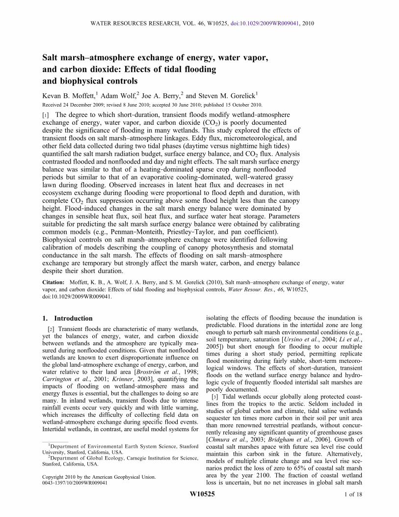
[7] The field site was a 0.9 ha intertidal salt marsh insouthern San Francisco Bay, within the Palo Alto BaylandsNature Preserve (37°27′54″N, 122°6′58″W, Figure 1). Thesite experiences mixed semidiurnal tides and a semiarid

Figure 1. Intertidal salt marsh field site map.

MOFFETT ET AL.: FLOOD EFFECTS ON SALT MARSH–ATMOSPHERE EXCHANGE W10525W10525

2 of 18

Mediterranean climate with winter precipitation (October toApril, ∼39 cm/yr). At 1.02 ± 0.06 m above local mean sealevel, the marsh plain is above mean high water and isflooded by the daily higher high tide on two thirds to threefourths of days during each 14 day spring‐neap cycle. Thesalinity of far southern San Francisco Bay water typicallyranges from ≥15 PSU during winter/spring rains to ≤30 PSUJune–December (1 PSU ≈ 1 g/L) [Schemel et al., 2003].Vegetation cover is complete and dominated in roughlysimilar proportion by the C4 grasses Spartina foliosa andDistichlis spicata and the C3 succulent Salicornia depressa(formerly S. virginica). The highest tides during the studyperiod submerged short Spartina sprouts and partially sub-merged taller Spartina, Salicornia, and Distichlis.[8] Wetland‐atmosphere fluxes are driven by incident

radiation. The net radiation (Rn) budget quantifies the netincoming shortwave radiation (downward Sd less upwardSu) and longwave (downward Ld less upward Lu) radiation(1). In wetlands, the surface is a combination of canopy,soil, and water, each of which have different thermal andreflectance properties.

Rn ¼ Sd � Su þ Ld � Lu ð1Þ

The surface energy balance quantifies the dissipation of netradiation (Rn) by ground heat conduction (G) and by latent(lE) and sensible (H) turbulent heat convection and can berearranged to compare the net available energy (AE) to theenergy dissipated by land‐atmosphere turbulent exchange(2). In this study, we further partitioned the ground heat fluxduring flooding into two components: soil heat flux (Gs) andthe change in surface water heat storage (DSw), combinedin series.

AE ¼ Rn � Gs �DSw ¼ H þ �E ð2Þ

[9] We quantified salt marsh–atmosphere exchange ofenergy, water, and CO2 using a suite of techniques tomeasure (1) radiation, (2) turbulent exchange of sensible andlatent heat and CO2, and (3) heat flux into the marsh surface(soil and water). Net radiation was calculated from mea-sured gross upwelling and downwelling fluxes of shortwaveand longwave radiation (measured with a Kipp & ZonenCNR1 net radiometer). Turbulent exchange of sensible andlatent heat and CO2 were measured using an eddy flux (EF)system, which calculates fluxes as the covariance betweenvertical wind speed and air temperature, water vapor con-tent, or CO2 concentration, for 30 min periods. Wind speedand temperature were measured using a 3‐D sonic ane-mometer (Campbell CSAT3) and volumetric concentrationsof CO2 and H2Ov were measured by a colocated fast‐response open‐path infrared gas analyzer (Licor LiI‐7500).To correct for systematic undermeasurement of daytimesensible and latent heat fluxes by the EF method, thesefluxes were scaled, preserving the midday Bowen ratio, asdiscussed by Twine et al. [2000]. Details of this scaling,EF data processing, energy balance closure, and turbulentcospectra quality are in the auxiliary material.1

[10] Soil heat flux (Gs) was measured as the heat flux at8 cm depth (Campbell HFP01SC) plus the change in heatstorage from 0 to 8 cm calculated using four thermocouples

placed at 2 and 6 cm depth (Campbell TCAV) in saturatedmarsh soils. The change in surface water heat storage (DSw)in wetland environments is difficult to constrain due to thesmall water volume and its transient advection [Drexleret al., 2004; Lafleur, 2008]. We calculated this change instorage as the residual of the marsh surface energy balancemeasured during flood events, since the other components ofequation (2) (Rn, Gs, H, lE) were all measured in the field.Additional methods to estimate DSw are contrasted in theauxiliary material.[11] Two evaporation pans were installed to directly

monitor potential evaporative flux. One pan was placed onthe levee adjacent to the salt marsh, 10 cm off the ground,on wooden supports. This pan, 0.5 m above the marshsurface and above the reach of the tide, was analogous topans employed in other intertidal marsh studies locatedamong dry upland land cover [e.g., Hughes et al., 2001]. Asecond pan was fitted with flotation devices and tetherednear the EF tower. The flotation height of this pan was suchthat the water surface in the pan was at nearly the sameheight as the flood waters but the pan was not inundated bythe tide. Between tides this pan rested on the marsh sedi-ments with its water surface among the vegetation (Spartinafoliosa) canopy. The two pans were monitored manually andrefilled with saline bay water as needed.[12] Ancillary meteorological data were measured at a

weather station 220 m from the EF tower in an adjacent,similar salt marsh (Onset HOBO Weather Station). The sta-tion recorded 10 min average measurements of downwellingshortwave radiation (separate from the measurements by thenet radiometer at the EF tower), air temperature, relativehumidity, horizontal wind speed, horizontal wind direction,and precipitation (none during study period). Data wererecorded continuously from 15–26 September 2008. Wecompared data from two study periods to assess the effectsof flooding high tides during the day (15–18 September)versus during the night (23–26 September).

2.2. Wetland‐Atmosphere Exchange Models

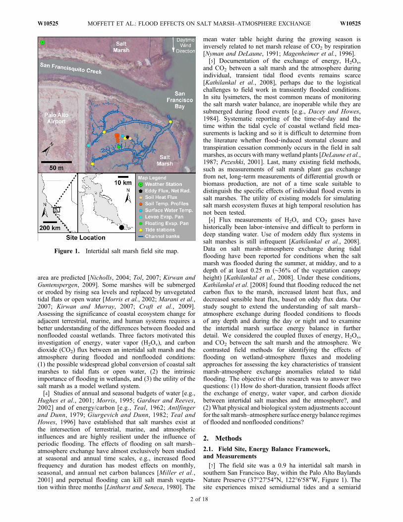
[13] Given the relative difficulty of routinely collectingeddy covariance data to characterize salt marsh–atmosphereexchange, compared to ease of obtaining micro-meteorological data, the utility of six micrometeorologicalmodels of land‐atmosphere exchange for describing theintermittently flooded salt marsh system were tested in thisstudy, summarized in Table 1. Four models are commonmethods primarily influenced by the radiation incident uponthe marsh surface. The few available calibrations of thesemodels for intertidal salt marshes are cited among theresults. Two additional models were constrained by leafbiochemical processes and were included in the analysis tobetter understand the relative role of plant physiologycompared to net radiation in controlling the salt marshsurface energy balance. Each of the six models simplifiedland‐atmosphere exchange via different key parameters,listed in the last column of Table 1.[14] The purpose of employing these six models was

threefold. First, we sought to assess the applicability tointertidal salt marshes of generic “wetland” model para-meterizations from the literature. To do so, we ran eachmodel in a forward sense, using literature values (listed inthe appendix) and temporally variable input from the field

1Auxiliary materials are available in the HTML. doi:10.1029/2009WR009041.


3 of 18

Tab

le1.

Suite

ofSix

Mod

elsof

Land‐Atm

osph

ereExchang

e:Abb

reviated

Descriptio

ns

Mod

elFormulae

aMajor

Features

Assum

ptions

TestsRoleOf

Energy‐DrivenMod

els

Priestley‐Taylor(PT)

[Priestleyan

dTaylor,19

72]

lEti=a′D

Dþ�AE

Radiatio

ndriven.Develop

edfor

saturatedland

andwater

surfaces.

Dandgdepend

onTa.

a′=1.26

.Positive

sensible

heat

flux

.Positive

vapo

rpressure

deficit(nocond

ensatio

n).b

radiativeforcing

parameter:a′

Penman‐M

onteith

(PM)

[Mon

teith

,19

65]

lEti=

AEDþ�

ac p

e Ta*�

e að

Þ=ra

Dþ�

1þr sc=r a

ðÞ

Radiatio

n‐and(e

Ta*−

e a)‐driven.

Aerod

ynam

icandsurface

resistance

effects.

“Big

leaf”cano

pyapprox

imation.

r aisa

functio

nof

uandh c.r scassumed

orfrom

porometer

data.b

boun

dary

layer

parameter:r sc

Wessel‐Rou

se(W

R)or

Weigh

tedPM

[Wesselan

dRou

se,19

94]

lEti=P j

wjlEj=LAI p

·lE

c+S·lE

s+W

·lE

w

lEj=

AEDþ�

ac p

e Ta*�

e að

Þ=ra

Dþ�

1þr sj=r a

ðÞ

Variablesurfacecover:cano

py(LAI p),

soil(S),andwater

(W)area

fractio

nsexplicitlyaccoun

tforpartialfloo

darea.Different

r sforeach

cover.

Parallel‐actin

gcoverfractio

ns.Projected

LAI p

representscano

pyfractio

ncontribu

tion.

Allfrom

Penman‐M

onteith

.b

fractio

nalcover,

cano

pyandsoilresistances

parameters:

r sc,r ss

Pan

Coefficient

(MPor

LP)

[Allenet

al.,19

98]

lEti=lr

wEti/100

0ti

Eti=E0·sin(t ip

/t d)/(2/p)

E0=K

·Epan

K=Kpan×Kcrop.K

scales

Epanto

wetland

cano

py.Normalized

sine

functio

ncreatesdiurnalvariationfrom

daily

E0.

RepresentativeK.MedianEpanfrom

fielddata.Sinusoidaldiurnalsign

al.

ambientcond

ition

s(levee

versus

marsh)

parameter:K

Bioph

ysical

Mod

els

C3Bioph

ysics(C

3)

[Collatzet

al.,19

91]

g sv=m

Anh s

Ccs

+b

E=g b

v(h

s·e T

l*−e a)/P

An=f(S d,LAI,Tl,leaf

biochemistry)

NEE=An−Reco=An(1

−b A

)

Light,Rub

isco,andsucrose‐prod

uctio

ncolim

itedC3ph

otosyn

thesisand

stom

atal

respon

se.

Ball‐Berry

mod

elparameters(m

,b).

Biochem

ical

parameter

values.Ecosystem

respirationin

prop

ortio

nto

An.

Soilcontribu

tionto

lEaccording

toBeer’senergy

transm

ission

law

and

leaf

area

indexLAI.

C3−versus

C4−biochemistry

parameters:

rate

limita

tion,

Vmstom

atal

control,

mecosystem

resp.,

b Asoilevap

.,LAI

C4Bioph

ysics(C

4)

[Collatzet

al.,19

92]

lE=a·E·

1þ

exp�0

:5�LA

Ið

Þ1�

exp�0

:5�LA

Ið

Þð

Þ�

�Light,Rub

isco,andsucrose‐prod

uctio

ncolim

itedC4ph

otosyn

thesisand

stom

atal

respon

se.

a The

App

endix(Table

A1)

contains

afulllistof

parameter

symbo

ls,variable

names,andspecifiedvalues.See

citatio

nsformod

eldetails.

bAssum

ptions

common

tothesemod

els:saturatedsurfaceat

Ta,lin

earizedsaturatio

nvapo

rpressure‐tem

perature

curve,

neutrally

stable

boun

dary

layer,AE=Rn−G

s−DS w

.


4 of 18

data (net radiation, ground heat flux, air temperature, pres-sure, and humidity). Second, we sought to produce a cali-brated suite of models to enable more accurate simulation ofthe intertidal salt marsh surface energy balance. We invertedthe models to calibrate key parameters for three scenarios:for all measurements, for intervals between tides, and forflooded periods. Third, we sought to compare the ensembleof calibrated parameters to better‐studied grassland‐likesystems in order to gain additional conceptual insight intothe prominent characteristics of salt marsh–atmosphereexchange and specific ways the exchange is altered bytransient flood events.

[15] The first four models represent the land‐atmosphereexchange of water via latent heat (lE) in linear proportion tothe net available energy (AE) or to the flux from an analogousevaporating (pan) system: the Priestley‐Taylor, Penman‐Monteith, Wessel‐Rouse, and pan coefficient models. Here-after we refer to these as the energy‐driven models. Wecalculated the modeled sensible heat flux (H) as the energybalance residual of the modeled bulk latent heat flux (lE)and the measured net radiation (Rn), soil heat flux (Gs),and residual change in surface water heat storage (DSw):i.e., only the lE and H components of the surface energybalance were modeled and the Rn, Gs, and DSw, componentstaken as equivalent to the measured values.

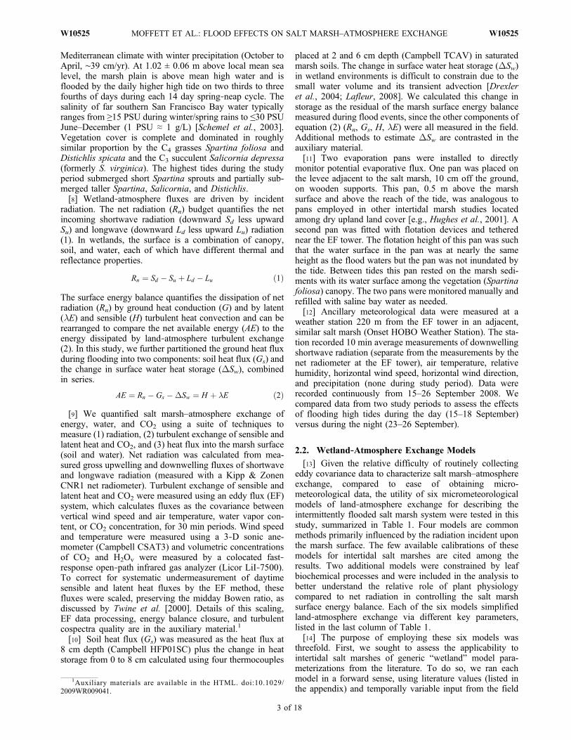
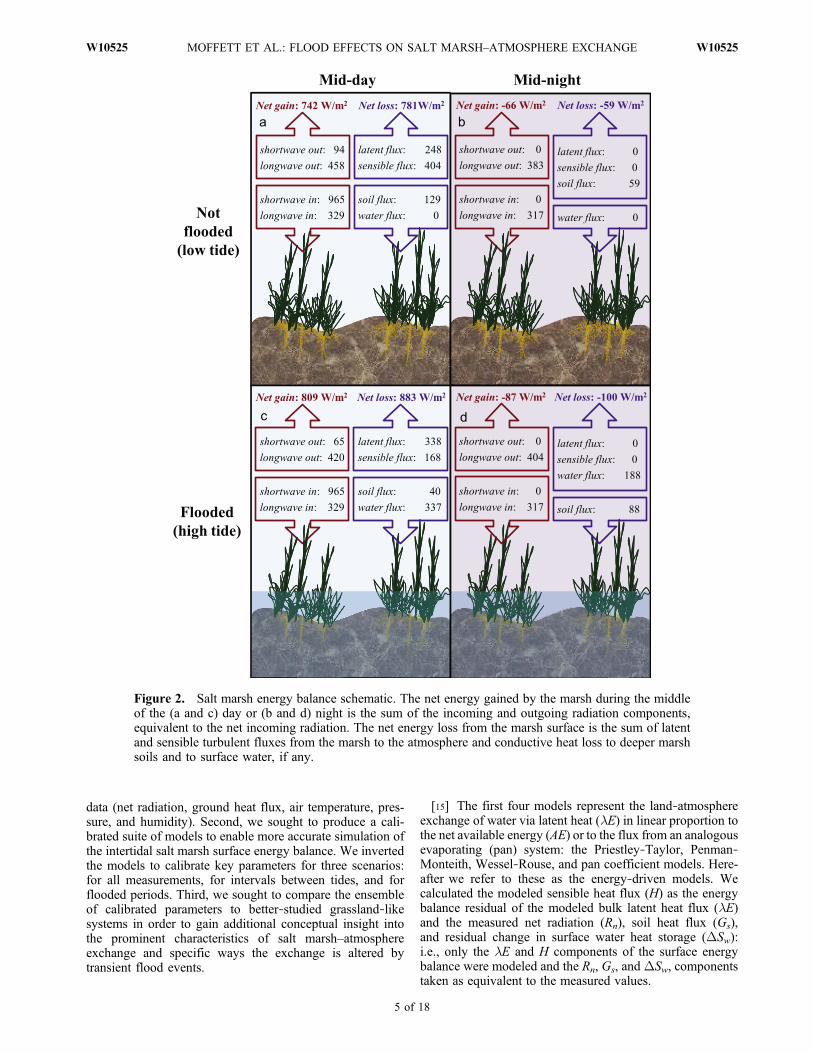
Figure 2. Salt marsh energy balance schematic. The net energy gained by the marsh during the middleof the (a and c) day or (b and d) night is the sum of the incoming and outgoing radiation components,equivalent to the net incoming radiation. The net energy loss from the marsh surface is the sum of latentand sensible turbulent fluxes from the marsh to the atmosphere and conductive heat loss to deeper marshsoils and to surface water, if any.


5 of 18

[16] The four energy‐driven models characterize the fluxof water by evapotranspiration as the product of the watervapor gradient between a saturated surface and an unsatu-rated atmosphere and a parameterized resistance to watervapor transport: explicitly, in the Penman‐Monteith andWessel‐Rouse models or implicitly, in the coefficients of thePriestley‐Taylor and pan coefficient models. The resistanceterm embodies the additional resistance imposed by thediffusion of water vapor from the interior of the leaf or thesoil subsurface to the bulk atmosphere. The resistance

imposed by the atmosphere is small for moderate‐to‐highwind speeds and the contribution from the soil may be smallwhen vegetation is dense. Under these conditions, thedominant control on H2Ov flux is stomatal conductance(gsv). Ball [1988] found a strong relationship between sto-matal conductance and the net photosynthetic rate of the leaf(An), the CO2 concentration at the leaf surface (Cs), and therelative humidity at the leaf surface (hs) (see Table 1), whichhas been validated for a wide variety of plant types. Becausethe leaf photosynthesis rate (An) is closely linked to light

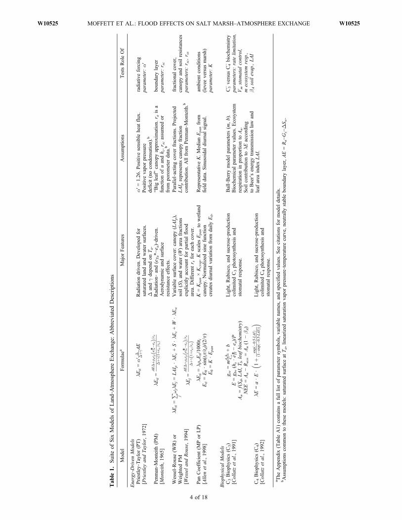
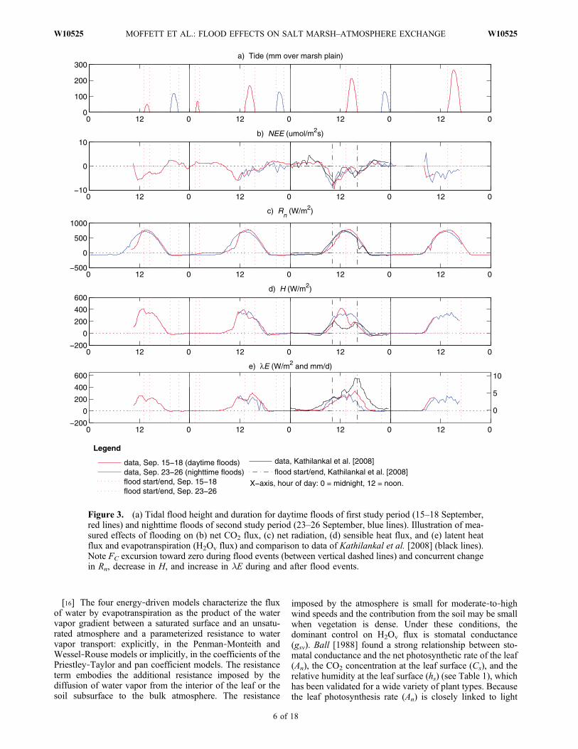
Figure 3. (a) Tidal flood height and duration for daytime floods of first study period (15–18 September,red lines) and nighttime floods of second study period (23–26 September, blue lines). Illustration of mea-sured effects of flooding on (b) net CO2 flux, (c) net radiation, (d) sensible heat flux, and (e) latent heatflux and evapotranspiration (H2Ov flux) and comparison to data of Kathilankal et al. [2008] (black lines).Note FC excursion toward zero during flood events (between vertical dashed lines) and concurrent changein Rn, decrease in H, and increase in lE during and after flood events.


6 of 18

availability and the leaf surface humidity is directly linked tothe radiation‐driven evaporation rate, the Ball‐Berry for-mulation of stomatal conductance enables coupling stomatalconductance to the surface energy balance, provided An canbe calculated. The resulting combined photosynthesis‐stomatal conductancemodel [Collatz et al., 1991, 1992] is nowa standard method for linking the land surface and atmo-sphere in climate models and represents a fundamentallydifferent modeling approach compared to the energy‐drivenmodels more often employed in hydrology. In the coupledmodel, stomatal conductance is calculated iteratively: aphotosynthesis model estimates successive values of An

[Farquhar et al., 1980] and the Ball‐Berry model estimatessuccessive values of stomatal conductance. The key param-eter in the photosynthesis model is the maximum carbox-ylation velocity (Vm) of the leaf (the enzymatic capacity tochemically fix CO2), which varies between species anddepends on the phenological state of the plant. The simu-lations of net photosynthesis (An) and transpiration from theleaf‐level coupled model are scaled to the canopy level by:(1) subtracting from An an estimate of nonleaf ecosystemrespiration (Reco) to calculate the canopy‐level net ecosys-tem exchange (NEE), and (2) weighting soil and leaf con-tributions to evapotranspiration according to Beer’s Law,which describes an exponential decrease in the amount ofenergy reaching the ground surface, scaled by the canopyleaf area index (LAI; see Table 1).[17] The biochemical parameters used in the photosyn-

thesis model were estimated by taking leaf chamber mea-surements of An at different light and CO2 levels for leavesof the C4 grasses Spartina foliosa and Distichlis spicata andphotosynthetic stems of the C3 succulent Salicornia depressa(Salicornia leaves are vestigial). The plants were takenfrom the field site with intact root systems in August 2008(2–3 weeks prior to the field study and a few days beforelaboratory measurements), kept in an outdoor greenhouseunder natural light, and watered periodically with bay water.Prior to measurement, the selected leaves/stems were wipedclean of salt with a damp cloth and allowed to air dry. Leafgas flux measurements (Licor LI‐6400) were recorded after30–50 min, once the fluxes had equilibrated to each changein light or CO2 level. The specific measurement techniquesand settings used for each plant species are described in theauxiliary material. The CO2 and light response curves wereanalyzed with standard nonlinear curve fitting software(Levenberg‐Marquart algorithm) to find the biochemicalparameters (e.g., Vm) that minimized the difference between

the observations and the Collatz et al. [1991, 1992] modelsfor C3 and C4 plants.

3. Field Results

3.1. Nonflooded Conditions

[18] During nonflooded conditions, the salt marsh exhib-ited a midday energy balance dominated by outgoinglongwave radiation reradiated from the surface, accountingfor 62% of the radiation budget, and by the turbulent dis-sipation of energy via the sensible heat flux, accounting for52% of the surface energy balance (Figure 2a). This char-acterization of the nonflooded marsh during the daytime as awarm surface with significant canopy reradiation is consis-tent with the canopy energy balance of Spartina alternifloraand S. patens studied by Teal and Kanwisher [1970]. Themagnitudes of latent and soil heat fluxes at midday duringnonflooded conditions (19% and 10% of net radiation,respectively) were smaller than the magnitudes of reradia-tion and sensible heat flux. The ambient CO2 concentrationin the air above the marsh during nonflooded conditionsexhibited a consistent diurnal cycle and measured net CO2

flux from the marsh also varied diurnally (Figure 3b). Theseresults were consistent with the average diurnal cycle of netCO2 flux during the growing season reported by Kathilankalet al. [2008]. Net photosynthetic CO2 uptake produced adownward (negative) flux during the day of up to 9.6mmol/m2/s(median 2.3 mmol/m2/s), with maximum flux occurring inthe late morning. This rate is comparable to NEE valuesreported by Cornell et al. [2007] for mature referencemarshes measured under full sunlight (3–12 mmol/m2/s).The energy balance of the nonflooded marsh during themiddle of the night (Figure 2b) continued the daytime trendof the salt marsh as a warm surface, dissipating most of itsheat load through reradiated thermal energy. The exposedsalt marsh soil that was a heat sink during the day became aheat source at night. Net CO2 release from soil and night-time plant respiration produced an upward (positive) flux atnight of up to 2.7 mmol/m2/s (median 1.0 mmol/m2/s), withmaximum flux occurring soon after sunset.

3.2. Effects of Flooding

[19] A major finding was a pronounced reduction in saltmarsh–atmosphere CO2 exchange during tidal flood eventsin proportion to flood duration, especially important giventhe role of salt marshes as carbon sinks [Chmura et al.,2003; Bridgham et al., 2006]. Although shallow middaytides of short duration only partially suppressed marsh‐atmosphere CO2 exchange (e.g., 15 and 16 September,Figure 3b), CO2 exchange between the atmosphere andmarsh was completely suppressed during the peak of longmidday flood events (e.g., 17 September, Figure 3b). Thisfinding was consistent with the similar finding ofKathilankalet al. [2008] that “Surface energy fluxes changed in responseto the tidal level, with increased latent heat and decreasedsensible heat fluxes occurring during the midday high tideevent. Tide‐induced changes in diurnal patterns of energyfluxes and reduction in the carbon fluxes were observedwhen unusually high tidal levels were recorded.” Ourquantitative finding that the degree of the suppression ofcarbon flux was directly proportional to flood duration anddepth was not previously reported by Kathilankal et al.

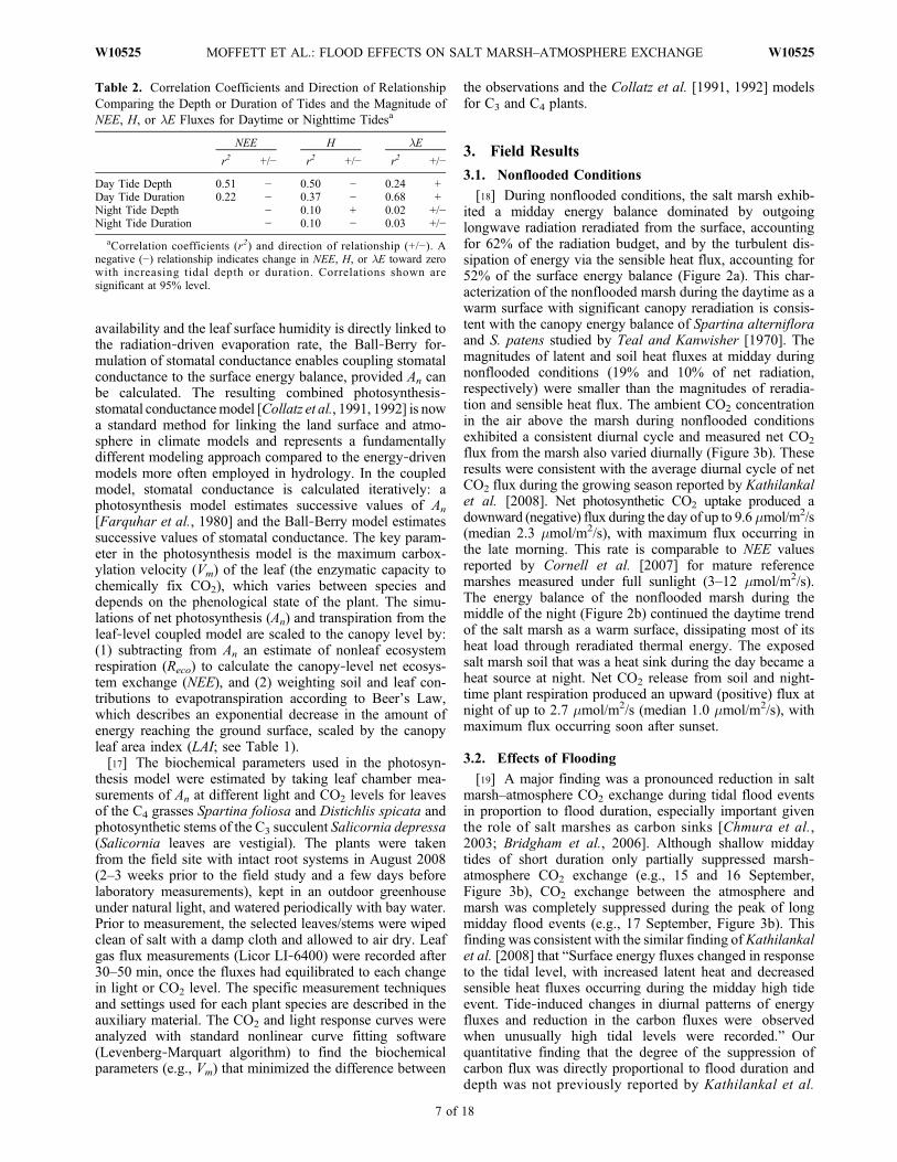
Table 2. Correlation Coefficients and Direction of RelationshipComparing the Depth or Duration of Tides and the Magnitude ofNEE, H, or lE Fluxes for Daytime or Nighttime Tidesa

NEE H lE

r2 +/− r2 +/− r2 +/−

Day Tide Depth 0.51 − 0.50 − 0.24 +Day Tide Duration 0.22 − 0.37 − 0.68 +Night Tide Depth − 0.10 + 0.02 +/−Night Tide Duration − 0.10 − 0.03 +/−

aCorrelation coefficients (r2) and direction of relationship (+/−). Anegative (−) relationship indicates change in NEE, H, or lE toward zerowith increasing tidal depth or duration. Correlations shown aresignificant at 95% level.


7 of 18

[2008] or other authors, however. Our data from nighttimeand early afternoon high tides contrasted with the finding ofKathilankal et al. [2008] that “[w]hen high tides did notoccur concurrently with midday peaks in solar irradiancelevels, no changes in diurnal carbon and energy fluxes wereobserved,” since we observed such changes both at nightand during the afternoon.[20] Further analyzing the apparent proportionality

between carbon flux suppression and tidal flooding, wefound that the flood‐induced suppression of midday CO2

flux was more strongly correlated with tidal depth thanduration (Table 2). The suppression of CO2 flux transitionedfrom partial to complete at a threshold between a floodduration of 2.47–2.80 h and a flood depth of 16.9–21.2 cm.This depth/duration threshold is curious compared to themaximum stem heights of key salt marsh species (Spartinafoliosa ∼40 cm, Salicornia depressa ∼30 cm [Rosso et al.,2006]). We attribute this phenomenon to the combinedeffects of the sudden, complete submergence of salt marshsoils, halting their large respiration flux, and the gradual,

Figure 4. (a) Tidal flood height and duration for daytime floods of first study period (15–18 September,red lines) and nighttime floods of second study period (23–26 September, blue lines). Measured effects offlooding on (b) upwelling longwave radiation, (c) upwelling shortwave radiation, (d) soil heat flux,(e) change in surface water heat storage, (f) air temperature, (g) soil temperature at 4 cm depth, (h) relativehumidity, and (i) horizontal wind speed.


8 of 18

lagged effects of progressive occlusion of the emergentvegetation. The effects of flooding on soil‐atmosphere CO2

exchange are consistent with evidence that just 1–2 mm offlood depth can begin to suppress sediment (algal) photo-synthesis by 48%–66% [Holmes and Mahall, 1982] and thatsurface flooding decreases respiration [Magenheimer et al.,1996]. We expect that the effects of flooding on theemergent vegetation are a nonlinear combination of indi-rect plant metabolism inhibition by soil water pressure orflood water temperature changes and direct partial sub-mergence, restricting the gas flux able to diffuse throughthe flood waters.[21] The latent heat flux and evapotranspiration between

the salt marsh and the atmosphere were also strongly cor-related with daytime flood event duration and depth, thoughmore strongly with tidal duration (Table 2). The data ofKathilankal et al. [2008] from a midday flood of longduration and substantial depth in a Virginia, USA, saltmarsh further support this observation, showing a propor-tionately greater effect of flooding on latent heat flux fortheir event of longer flood duration, compared to our fielddata (Figure 3e). The dependence of both CO2 and H2Ov

fluxes during flooding on the magnitude of the flood eventis consistent with the common influence of plant and soilmetabolic activity on both fluxes. However, in contrast tothe observed decrease in marsh‐atmosphere CO2 exchangeduring flood events, the latent heat flux increased at the endof, and following, daytime flood events. We attribute thisphenomenon to increased moisture availability and decreasedresistance to H2Ov transport from open water compared tosoil and plant leaves of magnitude large enough to offset thedecreases in transpiration that must occur concurrently withthe observed decreases in photosynthetic carbon uptake.Significantly, flood‐induced augmentation of latent heatflux and suppression of CO2 flux were observed eventhough the tidal stage remained beneath the vegetationcanopy at all times.[22] The large difference in H2Ov flux by evapotranspi-

ration during flooding compared to nonflooded conditionscontrasted with the prevalent conceptual model that the

evapotranspiration regime of salt marshes is very similar tothat of open water systems [Hussey and Odum, 1992]. Anumber of factors might distinguish salt marsh evapotrans-piration and open water evaporation rates for a particularcase study, e.g., air and water temperature differences,vegetation phenology, antecedent water and salt stress, soilmoisture, and canopy closure. Based on observations ofwetland latent heat flux and carbon exchange, it is alsopossible to estimate the amount of flux due to vegetationtranspiration versus soil or water undercanopy evaporation(E) as in equation (3). We first calculated total photosyn-thesis by subtracting from the measured net ecosystemcarbon exchange (NEE) the ecosystem respiration rate(Reco). We used the mean measured nighttime NEE rate(Reco = 0.86 mmol/ms/s, this study) as an estimate of theecosystem respiration rate, which is consistent throughoutthe day in many ecosystems. Laboratory measurements ofleaf gas flux yielded estimates of the leaf instantaneoustranspiration efficiency (ITE), the ratio of CO2 uptake toH2Ov loss via simultaneous molecular diffusion throughplant leaf stomata. Our laboratory data produced averageITE values of about −6 for Salicornia depressa, −12 forSpartina foliosa, and −9 for Distichlis spicata at ambientlight and CO2 levels, resulting in an area‐weighted averageestimate of ITE = −9 mmol CO2/mmol H2Ov for a marshcodominated by these three species. Our ITE estimates agreewell with those of other authors (e.g., ITE ≈ 10 mmol/mmol,Jiang et al. [2009] for Spartina alterniflora in China in latesummer; ITE ≈ 14 mmol/mmol, Teal and Kanwisher [1970]for Cape Cod Spartina alterniflora on a cool, humid day).Unit conversion of the calculated flux from mmol/m2/s toW/m2 completed the estimation of the amount of the latentheat flux associated with plant transpiration (3).

Transpiration latent energy ¼ NEEdaytime � Reco

ITE

� �� 18

106

� �

ð3Þ

According to this estimation method, we found that tran-spiration accounted for 13% of daytime latent heat flux inthe salt marsh, on average, and that this transpiration fluxwas suppressed during tidal flooding (along with NEE) evenas the evaporative portion of the latent heat flux increasedduring and following marsh flooding.[23] In addition to tidal effects on CO2 and H2Ov fluxes,

tidal flooding significantly increased the total magnitude ofenergy exchanged between the marsh and the atmosphereand changed the relative importance of each of the energybalance components (Figures 2c and 2d). The correlationbetween the decrease in the sensible heat flux from themarsh and tidal depth and duration was also significant,more strongly correlated with tidal depth than durationduring the day (Table 2). We attribute this phenomenon tothe prolonged exposure of the marsh to tidal waters that hada higher (nighttime) or lower (daytime) surface temperaturethan the air and marsh surface. Due to the small magnitudesof sensible and latent heat flux at night, the correlationsbetween these fluxes and tidal depth and duration at nightwere inconclusive. Flooding also induced subtle changes inambient atmospheric conditions (wind speed, air tempera-ture, relative humidity). The energy balance results areillustrated in Figures 2–4 and summarized in Table 3, andthe maximum effects are described in the following.

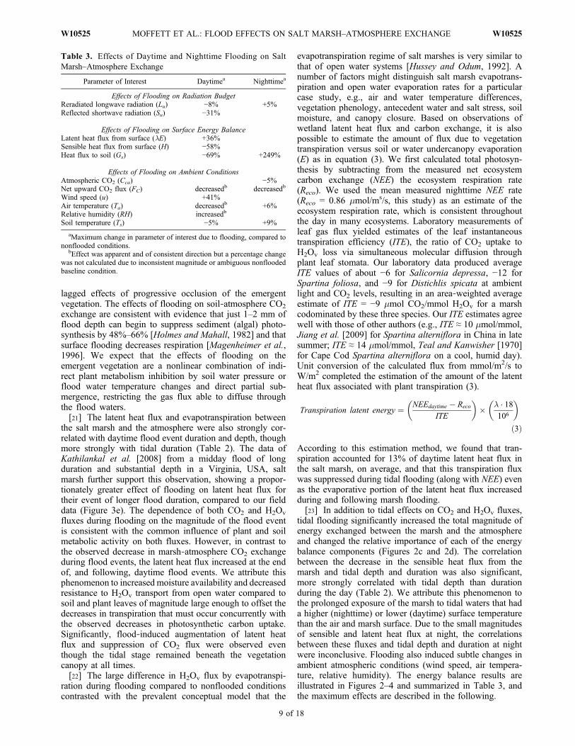
Table 3. Effects of Daytime and Nighttime Flooding on SaltMarsh–Atmosphere Exchange

Parameter of Interest Daytimea Nighttimea

Effects of Flooding on Radiation BudgetReradiated longwave radiation (Lu) −8% +5%Reflected shortwave radiation (Su) −31%

Effects of Flooding on Surface Energy BalanceLatent heat flux from surface (lE) +36%Sensible heat flux from surface (H) −58%Heat flux to soil (Gs) −69% +249%

Effects of Flooding on Ambient ConditionsAtmospheric CO2 (Cca) −5%Net upward CO2 flux (FC) decreasedb decreasedb

Wind speed (u) +41%Air temperature (Ta) decreasedb +6%Relative humidity (RH) increasedb

Soil temperature (Ts) −5% +9%

aMaximum change in parameter of interest due to flooding, compared tononflooded conditions.

bEffect was apparent and of consistent direction but a percentage changewas not calculated due to inconsistent magnitude or ambiguous nonfloodedbaseline condition.


9 of 18

[24] During midday tidal flooding the salt marsh was acool, wet surface, in contrast to its warm‐surface character-istics during nonflooded conditions. Flooding effected a 10%increase in the net radiation incident upon the marsh surfacevia reductions in surface‐emitted longwave radiation and insurface‐reflected shortwave radiation (Figures 4b and 4c).The decrease in reflected shortwave radiation during floodswas associated with a reduction in the minimum daily albedofrom 0.089 during nonflooded conditions to 0.073 duringflooded conditions. During midday floods, the increased heatload due to the net radiation increase was augmented by largeconcurrent reductions in sensible heat flux (Figure 3d) and insoil heat flux from the marsh surface (Figure 4d). The surfaceenergy balance was maintained by a large, temporary heatflux into the flood waters (Figure 4e) and an increase in thelatent heat flux from the marsh during and after the floods(Figure 3e).[25] At night, the warm tidal waters increased the amount

of longwave radiation reradiated by the marsh surfacecompared to nonflooded conditions and so reduced the netradiation peak by 32%. Nighttime flooding by tidal waterswarmer than the air also reversed the direction and increasedthe magnitude of the soil heat flux (Figures 3d and 4d). Theenergy for these changes was supplied by the warm tidalwaters, which we conceptualize as a capacitor that is pro-gressively “charged” with heat during the day (whileexposed as a shallow layer over the marshes and mudflats)that is released to the marsh and air during high tides,especially at night.[26] Additional indirect effects of flooding on marsh‐

atmosphere linkages appeared in the data on wind speed,ambient air temperature, and relative humidity during floodevents. Nongust wind speeds during midday flood eventswere up to 41% greater than during similar nonflooded per-iods, perhaps due to decreased roughness of mudflats and saltmarshes in the fetch area during flooding (Figure 4i). Despitepatently different air temperatures between the first (15–18 September) and second (23–26 September) study periods,small anomalies in the shape of the air temperature historyoccurred coincidentally with the times of floods on almostevery date (Figure 4f). Nighttime flooding by water warmerthan the air slightly increased air temperature, due to the large,temporary heat flux from flood waters to the atmosphere; thiseffect was large enough to quantify (Table 3). This repeated,transient phenomenon qualitatively confirmed that floodingof the marsh by water at a different temperature than the airand marsh subtly changed air temperatures according to thechange in the sensible heat flux. Despite distinctly differentmidday relative humidity between the first and second study

periods, small positive anomalies in the relative humidityhistory coincided with the times of midday floods, likely aconsequence of the increased evaporation and altered airtemperature at these times (Figure 4h). For the short‐durationflood events of this study, these indirect effects of floodingon the environmental conditions surrounding the marshsystem were slight, transient, and rapidly reversible; forlonger‐duration flood events, however, such changes inambient atmospheric conditions might feed back on marsh–atmosphere exchange, further altering the balance of heat,water, and carbon exchange between the marsh and theatmosphere.

4. Energy‐Driven Simulation Results

[27] Energy‐driven exchange between our intermittentlyflooded salt marsh site and the atmosphere was poorlyrepresented by forward simulations based on parametervalues obtained from the literature for wetlands. ThePriestley‐Taylor (PT), Penman‐Monteith (PM), and Wessel‐Rouse (WR) models consistently overpredicted the averagedaily latent heat flux, failing to adequately describe thepartitioning of the surface energy balance in the salt marsheven during nonflooded conditions. The best of the forwardmodel results were from the pan coefficient model based onthe median measured evaporation rate from the floatingevaporation pan deployed among the marsh vegetation(MP). The pan coefficient models produced fluxes ofappropriate average magnitudes and exhibited strong cor-relations with the eddy flux data time series’.[28] We used our field data to invert the energy‐driven

models and calibrate key parameters. For each energy‐driven model, we found the three parameter sets that best fitthree different subsets of the field data, from (1) nonfloodedperiods only, (2) flooded periods only, and (3) all timesduring the study period. The PT, PM, and pan coefficientmodels were inverted by solving for the parameter ofinterest (listed in Table 1, last column) as the slope of a bestfit line to the lE data with an intercept of zero. To calculatethe two parameters of interest in the WR model we foundthe parameter pair that minimized the sum of squared dif-ferences between the model results and field data.[29] Following calibration via these inversions, the PT,

PM, and WR model estimates of average salt marsh–atmosphere fluxes compared well with the field data(Table 4). The initially good flux estimates from the pancoefficient method were fine tuned by calibration to bettermatch the field data. (Because the MP and LP pans bothwere modeled based on scalar median evaporation rates,separate linear calibration of the two pans resulted in

Table 4. Calibrated Energy‐Driven Flux Model Resultsa

Model E (mm/d)

lE H NEE

W/m2 r2 W/m2 r2 mmol/m2s r2

Eddy flux (data) 2.69 146 1.00 159 1.00 −1.96 1.00Priestley‐Taylor (PT) 2.31 125 0.74 180 0.89 −1.31 0.24Penman‐Monteith (PM) 2.72 147 0.59 157 0.85 −1.54 0.13Wessel‐Rouse (WR) 2.38 129 0.62 176 0.84 −1.34 0.18Marsh Pan Coefficient (MP) 2.65 144 0.78 161 0.81 −1.51 0.39Levee Pan Coefficient (LP) 2.65 144 0.78 161 0.81 −1.51 0.39

aModeled mean daily average daytime evapotranspiration (E), latent heat (lE), sensible heat (H), and net carbon (NEE) fluxes and correlationcoefficients (r2) between the modeled flux time series’ and the field data. These results are calculated by applying calibrated parameters derived fornonflooded conditions only to nonflooded time periods and calibrated parameters derived for flooded conditions only to flooded time periods.


10 of 18

identical calibrated flux results.) The pan coefficientmodels provided the best fit to the eddy covariance dataafter calibration. Parameter calibration served mainly toreduce the estimate of available energy dissipation bylatent heat flux in the four energy‐balance models.Detailed model results and correlations between the fielddata and the precalibration and postcalibration results areillustrated in the auxiliary material.

4.1. Energy‐Driven Exchange: Nonflooded Conditions

[30] The energy‐driven simulation results suggested aconceptual model of the surface energy balance of a non-flooded salt marsh as similar to that of a sparse crop. Theinverted PM andWRmodels required high canopy resistancesto H2Ov transport (rsc, 171 to 248 s/m, Table 5) to match thefield data, comparable to those used by Shuttleworth andWallace [1985] for sparse crops: if adjusted to a LAI ≈ 1,their rsc = 200 s/m. These values were much higher than theinitial rsc = 5 s/m value we tested [after Hughes et al., 2001].The magnitudes of the best fit canopy resistances suggestedthat the “big‐leaf” approximation of the PM model and thesmall soil contribution permitted in the WR model by its areaweighting method were both poor approximations of the saltmarsh. The persistently high water content of the marsh soilsand their potential to host microphytobenthic algae may haveaugmented the role of the soil in the overall salt marsh–atmosphere transaction measured by the field data. The“sparse crop” interpretation is supported by the similarity ofthemagnitudes of the best fit soil and canopy resistances in theWRmodel, indicating that canopy and soil contributions to thelatent heat flux were both important in the marsh water bal-ance. Alternatively, large canopy resistances could be due toplant water limitation (e.g., by soil salinity or hot, dry winds)or to leaf maturity and senescence [Monteith, 1965], but thesepossibilities are less well supported by our field observationsthan the sparse crop‐like conceptual model.[31] We found that salt marsh latent heat flux during

nonflooded conditions was not as strongly driven by theavailable radiation as in other open water and wetlandexamples. This observation was based on the calibratedPriestley‐Taylor (PT) model, which required a significantlyreduced scaling coefficient (a′, Table 5) to match the fielddata. In comparison, a′ values greater than one are typicalfor open water and wetlands [Priestley and Taylor, 1972].Low soil moisture, often invoked to explain low a′ values,did not occur in our salt marsh. Although salt‐induced saltmarsh water stress has been hypothesized, salt marsh plant

species are generally well enough adapted to the salineenvironment to avoid physiological drought [Kuramoto andBrest, 1979; Drake, 1989]. Our calibrated a′ values weresimilar to those reported by German [2000] for the FloridaEverglades. German suggested that low a′ values used tomodel flooded Everglades grasslands represented a largefraction of the radiation load being partitioned to heatingplants, soil, and debris and so elevating the sensible heatflux (H) relative to the latent heat flux (lE). This explana-tion of a heating‐dominated nonflooded salt marsh ecosys-tem was supported at our salt marsh site by a measuredmedian daytime Bowen ratio greater than unity (b = H/lE =1.20) and median partitioning of only 42% of availableenergy into latent heat flux during nonflooded conditionsand is consistent with our parsimonious conceptual model ofthe nonflooded salt marsh as if a “sparse crop” canopy.

4.2. Energy‐Driven Exchange: Flooded Conditions

[32] During flooded conditions, the ensemble of cali-brated model parameter values described a system in manyways opposite to the nonflooded salt marsh. Instead of largecanopy resistances to H2Ov exchange, the inverted PM andWR models best matched the field data using values similarto the standard reference crop value (our rsc = 67 to 74 s/mcompared to rsc = 70 s/m [Allen et al., 1998]). This resultsuggested that transient floods temporarily converted themarsh surface energy balance to be more similar to that ofwell watered short grass than a sparse crop. A larger PTcoefficient (a′) during flooding was consistent with a mea-sured median daytime Bowen ratio below unity (b = 0.92) atthese times and with the majority of available energy (52%)being partitioned into measureable latent heat flux. The pancoefficients resulting from model calibration to floodedconditions also suggested significant energy was partitionedinto latent heat flux during flooding.[33] These multiple phenomena suggest a temporary

regime shift during flooding from a nonflooded salt marshinfluenced by net heating to a flooded salt marsh experi-encing net evaporative cooling. At our site, this regime shiftoccurred despite the significant temporary heat uptake of thesurface water, which doubled the amount of availableenergy partitioned to the salt marsh substrate (soil and/orwater) during midday flood events. Even as the latent heatflux and evapotranspiration from the marsh increased duringand after flooding, CO2 flux was decreased.

Table 5. Calibrated Energy‐Driven Flux Model Parameters

Model Symbol Parameter Literature ValueaCalibrated Value

UnitsOverall Nonflooded Flooded

Priestley‐Taylor Flux Model a′ Priestley‐Taylor coefficient 1.26 0.598 0.576 0.734Penman‐Monteith Flux Model rsc median resistance to heat transfer

from canopy surface5 162 171 74 s/m

Wessel‐Rouse Flux Model rsc median resistance to heat transferfrom canopy surface

5 248 67 s/m

rss median resistance to heat transferfrom exposed soil surface

500 268 s/m

Pan Coefficient Flux Model:In‐Marsh Pan

K pan × crop coefficient 0.78 1.02 0.98 1.14

Pan Coefficient Flux Model:Nearby Pan on Levee

K pan × crop coefficient 0.78 0.56 0.55 0.64

aSee Table A1 for citations.


11 of 18

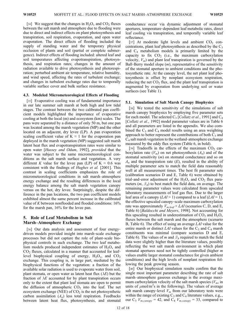
[34] We suggest that the changes in H2Ov and CO2 fluxesbetween the salt marsh and atmosphere due to flooding weredue to direct and indirect effects on plant photosynthesis andtranspiration, soil respiration, evaporation, and open waterevaporation. The direct effects of flooding included thesupply of standing water and the temporary physicalocclusion of plants and soil (partial or complete submer-gence). Indirect effects of flooding included: altered leaf andsoil temperatures affecting evapotranspiration, photosyn-thesis, and respiration rates; changes in the amount ofradiation available to drive photosynthesis and photorespi-ration; perturbed ambient air temperature, relative humidity,and wind speed, affecting the rates of turbulent exchange;and changes in turbulent exchange rates due to temporallyvariable surface cover and bulk surface resistance.

4.3. Modeled Micrometeorological Effects of Flooding

[35] Evaporative cooling was of fundamental importancein our late summer salt marsh at both high and low tidalstages. The contrast between the two calibrated pan coeffi-cient models highlighted the importance of evaporativecooling at both the local (m) and ecosystem (km) scales. Thepans were separated by a distance of only 50 m, but one panwas located among the marsh vegetation (MP) and the otherlocated on an adjacent, dry levee (LP). A pan evaporationscaling coefficient value of K ≈ 1 for the evaporation pandeployed in the marsh vegetation (MP) suggested salt marshlatent heat flux and evapotranspiration rates were similar toopen water [Hussey and Odum, 1992], provided that thewater was subject to the same micrometeorological con-ditions as the salt marsh surface and vegetation. A verydifferent K value for the levee pan (LP) of K ≈ 0.6 wasconsistent with the findings of Hughes et al. [2001]. Thiscontrast in scaling coefficients emphasizes the role ofmicrometeorological conditions in salt marsh–atmosphereenergy exchange and the resulting differences in the localenergy balance among the salt marsh vegetation canopyversus on the hot, dry levee. Surprisingly, despite the dif-ference in the pan locations, the two pan coefficient modelsexhibited almost the same percent increase in the calibratedvalue of K between nonflooded and flooded conditions: 16%for the marsh pan, 16% for the levee pan.

5. Role of Leaf Metabolism in SaltMarsh–Atmosphere Exchange

[36] Our data analysis and assessment of four energy‐driven models provided insight into marsh‐scale exchangeprocesses but did not capture the role of plant‐scale bio-physical controls in such exchange. The two leaf metabo-lism models produced independent estimates of H2Ov andCO2 fluxes, calculated in a manner that accounted for leaf‐level biophysical coupling of energy, H2Ov, and CO2

exchange. This coupling is, in large part, mediated by thebiophysical functions of the vegetation: a fraction of theavailable solar radiation is used to evaporate water from soil,plant stomata, or open water as latent heat flux (lE) but thefraction of lE accounted for by plant transpiration occursonly to the extent that plant leaf stomata are open to permitthe diffusion of atmospheric CO2 into the leaf. The netecosystem exchange (NEE) of CO2 is the net photosyntheticcarbon assimilation (An) less total respiration. Feedbacksbetween latent heat flux, photosynthesis, and stomatal

conductance occur via dynamic adjustment of stomatalapertures, temperature‐dependent leaf metabolic rates, directleaf cooling via transpiration, and temporally variable leafreflectance.[37] At moderate light levels and ambient CO2 con-

centrations, plant leaf photosynthesis as described by the C3

and C4 metabolism models is primarily limited by thecapacity to fix CO2 (i.e., the maximum carboxylationvelocity, Vm) and plant leaf transpiration is governed by theBall‐Berry model slope (m), representative of the sensitivityof the stomatal aperture to ambient conditions and the pho-tosynthetic rate. At the canopy level, the net plant leaf pho-tosynthesis is offset by nonplant ecosystem respiration,reducing the net CO2 flux, and the plant leaf transpiration isaugmented by evaporation from underlying soil or watersurfaces (see Table 1).

5.1. Simulation of Salt Marsh Canopy Biophysics

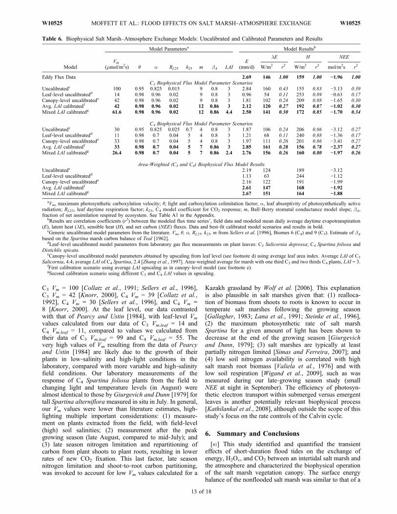
[38] We tested the sensitivity of the simulations of saltmarsh canopy biophysics by employing five parameter setsfor each model. The selected C3 [Collatz et al., 1991] and C4

[Collatz et al., 1992] model parameter values are in Table 6and all parameters are listed in the appendix. We also com-bined the C3 and C4 model results using an area weightingapproach to better represent the contributions of both C3 andC4 salt marsh vegetation to the wetland‐atmosphere exchangemeasured by the eddy flux system (Table 6, in bold).[39] Tradeoffs in the effects of the maximum CO2 car-

boxylation rate (Vm) on net photosynthesis (An) and of thestomatal sensitivity (m) on stomatal conductance and so onAn and the transpiration rate (E), resulted in the ability ofmultiple parameter sets to match the field data reasonablywell at all measurement times. The best fit parameter sets(calibration scenarios D and E, Table 6) were obtained bytrial‐and‐error adjustment of the H2Ov and CO2 flux para-meters (m, bA) to best match the field data, on average. Theremaining parameter values were calculated from upscaledlaboratory measurements of leaf gas flux. Due to the largerleaf area of a canopy (LAI > 1) compared to a leaf (LAI = 1),the effective upscaled canopy‐scale maximum carboxylationrate was approximately Vm,leaf × LAI (scenarios C, D, and E,Table 6) [Baldocchi and Meyers, 1998]. Not accounting forthis upscaling resulted in underestimation of CO2 and H2Ov

fluxes between the salt marsh and the atmosphere (scenarioB, Table 6). The effect of using an average LAI value for theentire marsh or distinct LAI values for the C3 and C4 marshconstituents was minimal (compare scenarios D and E,Table 6). The values of m and bA required to match the fielddata were slightly higher than the literature values, possiblyreflecting the wet salt marsh environment in which plantstomatal apertures need not be tightly controlled (higher mvalues enable larger stomatal conductance for given ambientconditions) and the high levels of nonplant respiration fol-lowing the peak growing season.[40] Our biophysical simulation results confirm that the

single most important parameter describing the rate of saltmarsh–atmosphere gaseous exchange is the average maxi-mum carboxylation velocity of the salt marsh species (Vm, inunits of mmol/m2s in the following). The values of averagesalt marsh canopy‐level Vm from our laboratory tests werewithin the range of existing C3 and C4 literature values, e.g,.,our C3 Vm,canopy = 42, and C4 Vm,canopy = 33, compared to


12 of 18

C3 Vm = 100 [Collatz et al., 1991; Sellers et al., 1996],C3 Vm = 42 [Knorr, 2000], C4 Vm = 39 [Collatz et al.,1992], C4 Vm = 30 [Sellers et al., 1996], and C4 Vm =8 [Knorr, 2000]. At the leaf level, our data contrastedwith that of Pearcy and Ustin [1984], with leaf‐level Vm

values calculated from our data of C3 Vm,leaf = 14 andC4 Vm,leaf = 11, compared to values we calculated fromtheir data of C3 Vm,leaf = 99 and C4 Vm,leaf = 55. Thevery high values of Vm resulting from the data of Pearcyand Ustin [1984] are likely due to the growth of theirplants in low‐salinity and high‐light conditions in thelaboratory, compared with more variable and high‐salinityfield conditions. Our laboratory measurements of theresponse of C4 Spartina foliosa plants from the field tochanging light and temperature levels (in August) werealmost identical to those by Giurgevich and Dunn [1979] fortall Spartina alterniflora measured in situ in July. In general,our Vm values were lower than literature estimates, high-lighting multiple important considerations: (1) measure-ment on plants extracted from the field, with field‐level(high) soil salinities; (2) measurement after the peakgrowing season (late August, compared to mid‐July); and(3) late season nitrogen limitation and repartitioning ofcarbon from plant shoots to plant roots, resulting in lowerrates of new CO2 fixation. This last factor, late seasonnitrogen limitation and shoot‐to‐root carbon partitioning,was invoked to account for low Vm values calculated for a

Kazakh grassland by Wolf et al. [2006]. This explanationis also plausible in salt marshes given that: (1) realloca-tion of biomass from shoots to roots is known to occur intemperate salt marshes following the growing season[Gallagher, 1983; Lana et al., 1991; Steinke et al., 1996],(2) the maximum photosynthetic rate of salt marshSpartina for a given amount of light has been shown todecrease at the end of the growing season [Giurgevichand Dunn, 1979]; (3) salt marshes are typically at leastpartially nitrogen limited [Simas and Ferreira, 2007]; and(4) low soil nitrogen availability is correlated with highsalt marsh root biomass [Valiela et al., 1976] and withlow soil respiration [Wigand et al., 2009], such as wasmeasured during our late‐growing season study (smallNEE at night in September). The efficiency of photosyn-thetic electron transport within submerged versus emergentleaves is another potentially relevant biophysical process[Kathilankal et al., 2008], although outside the scope of thisstudy’s focus on the rate controls of the Calvin cycle.

6. Summary and Conclusions

[41] This study identified and quantified the transienteffects of short‐duration flood tides on the exchange ofenergy, H2Ov, and CO2 between an intertidal salt marsh andthe atmosphere and characterized the biophysical operationof the salt marsh vegetation canopy. The surface energybalance of the nonflooded salt marsh was similar to that of a

Table 6. Biophysical Salt Marsh–Atmosphere Exchange Models: Uncalibrated and Calibrated Parameters and Results

Model

Model Parametersa Model Resultsb

Vm

(mmol/m2s) � a Rf,25 k25 m bA LAIE

(mm/d)

lE H NEE

W/m2 r2 W/m2 r2 mol/m2s r2

Eddy Flux Data 2.69 146 1.00 159 1.00 −1.96 1.00C3 Biophysical Flux Model Parameter Scenarios

Uncalibratedc 100 0.95 0.825 0.015 9 0.8 3 2.84 160 0.43 155 0.83 −3.13 0.39Leaf‐level uncalibratedd 14 0.98 0.96 0.02 9 0.8 3 0.96 54 0.11 253 0.89 −0.63 0.17Canopy‐level uncalibratede 42 0.98 0.96 0.02 9 0.8 3 1.81 102 0.24 209 0.88 −1.65 0.30Avg. LAI calibratedf 42 0.98 0.96 0.02 12 0.86 3 2.12 120 0.27 192 0.87 −1.02 0.30Mixed LAI calibratedg 61.6 0.98 0.96 0.02 12 0.86 4.4 2.50 141 0.30 172 0.85 −1.70 0.34

C4 Biophysical Flux Model Parameter ScenariosUncalibratedc 30 0.95 0.825 0.025 0.7 4 0.8 3 1.87 106 0.24 206 0.86 −3.12 0.27Leaf‐level uncalibratedd 11 0.98 0.7 0.04 5 4 0.8 3 1.21 68 0.11 240 0.88 −1.36 0.17Canopy‐level uncalibratede 33 0.98 0.7 0.04 5 4 0.8 3 1.97 111 0.26 201 0.86 −3.41 0.27Avg. LAI calibratedf 33 0.98 0.7 0.04 5 7 0.86 3 2.85 161 0.28 156 0.78 −2.37 0.27Mixed LAI calibratedg 26.4 0.98 0.7 0.04 5 7 0.86 2.4 2.76 156 0.26 160 0.80 −1.97 0.26

Area‐Weighted (C3 and C4) Biophysical Flux Model ResultsUncalibratedc 2.19 124 189 −3.12Leaf‐level uncalibratedd 1.13 63 244 −1.12Canopy‐level uncalibratede 2.16 122 191 −1.99Avg. LAI calibratedf 2.61 147 168 −1.92Mixed LAI calibratedg 2.67 151 164 −1.88

aVm, maximum photosynthetic carboxylation velocity; �, light and carboxylation colimitation factor; a, leaf absorptivity of photosynthetically activeradiation; Rf,23, leaf daytime respiration factor; k25, C4 model coefficient for CO2 response; m, Ball‐Berry stomatal conductance model slope; bA,fraction of net assimilation respired by ecosystem. See Table A1 in the Appendix.

bResults are correlation coefficients (r2) between the modeled flux time series’, field data and modeled mean daily average daytime evapotranspiration(E), latent heat (lE), sensible heat (H), and net carbon (NEE) fluxes. Data and best‐fit calibrated model scenarios and results in bold.

cGeneric uncalibrated model parameters from the literature. Vm, �, a, Rf,25, k25, m from Sellers et al. [1996], Biomes 6 (C4) and 9 (C3). Estimate of bAbased on the Spartina marsh carbon balance of Teal [1962].

dLeaf‐level uncalibrated model parameters from laboratory gas flux measurements on plant leaves: C3 Salicornia depressa; C4 Spartina foliosa andDistichlis spicata.

eCanopy‐level uncalibrated model parameters obtained by upscaling from leaf level (see footnote d) using average leaf area index. Average LAI of C3

Salicornia, 4.4; average LAI of C4 Spartina, 2.4 [Zhang et al., 1997]. Area‐weighted average for marsh with one third C3 and two thirds C4 plants, LAI = 3.fFirst calibration scenario using average LAI upscaling as in canopy‐level model (see footnote e).gSecond calibration scenario using different C3 and C4 LAI values in upscaling.


13 of 18

Table A1. Parameter Symbols and Values Used in the Text and Flux Models

Symbol Variable Source or Citation Valuea Units

Radiation BudgetRn net radiation W/m2

Sd downward (solar) shortwave radiation W/m2

Su upward (reflected) shortwave radiation W/m2

Ld downward (sky‐emitted) longwave radiation W/m2

Lu upward (reflected + ground‐emitted)longwave radiation

W/m2

Surface Energy BalanceH sensible heat flux W/m2

lE latent heat flux W/m2

G ground heat flux (soil + water components) W/m2

Gs soil heat flux W/m2

DSw change in surface water heat storage W/m2

AE net available energy, AE = Rn − G W/m2

Priestley‐Taylor Flux ModellEti “instantaneous” modeled latent heat flux

of time step tiW/m2

a′ Priestley‐Taylor coefficient Priestley and Taylor [1972] 1.26D slope of saturation vapor pressure‐temperature

curve at Ta, D = f (Ta, RH)Shuttleworth [1993, equation 4.2.3] Pa/°C

g psychrometric constant, g = f (Tws, P) Shuttleworth [1993, equation 4.2.28] Pa/°C

Penman‐Monteith Flux Modelra air density, ra = f (Ta, P) Shuttleworth [1993, equation 4.2.4] kg/m3

cp specific heat of dry air at constant pressure 1013 J/kg/°CeTa* saturation water vapor pressure at

Ta, eTa* = f(Ta)Shuttleworth [1993, equation 4.2.2] Pa

Ta ambient air temperatureb °Cu wind speedc m/sea ambient (air) water vapor pressure d,

ea = RH × eTa*Pa

ra aerodynamic resistance to heat transferfrom canopy to air,ra = f (canopy height, u, u height)

Shuttleworth [1993, equation 4.2.25] s/m

rs resistance to heat transfer from soil surface Hughes et al. [2001] 5 s/m

Wessel‐Rouse Flux ModelLAIp projected leaf area index (i.e., canopy area fraction) 0.95S exposed soil area fraction, S = 0 if flooded,

S = 1 − LAIp if not flooded0 or 0.05

W open water area fraction, W = 1 − LAIp if flooded,W = 0 if not flooded

0 or 0.05

rsc resistance to heat transfer from canopy surface Hughes et al. [2001] 5 s/mrss resistance to heat transfer from exposed soil surface Shuttleworth and Wallace [1985] 500 s/mrsw resistance to heat transfer from open water surface Shuttleworth and Wallace [1985] 0 s/m

Pan Coefficient Flux ModelEpan measured pan evaporation rate median of pan data mm/dKp pan coefficient Allen et al. [1998, ch. 4, Table 5] 0.65Kc crop coefficient Allen et al. [1998, Table 12,

midseason wetlands]1.20

K combined coefficient, K = Kp × Kc Allen et al. [1998] 0.78E0 daily pan‐reference evapotranspiration rate mm/dti time step of input data and model output 2 mintd length of daylight from radiometer data min

C3 Plant Leaf Metabolism Flux Modelg

Tl leaf temperaturee °CP ambient atmospheric pressuref PaE instantaneous transpiration H2Ov flux,

E = gtv (eTl* − ea)/Pmol/m2/s

gsv stomatal conductance to H2Ov mol/m2/sAn net assimilation (CO2 fixation) mmol/m2/shs humidity at leaf surfaceCcs leaf surface CO2 concentration mmol/molgbv boundary layer conductance to H2Ov Campbell and Norman [1998, 7.33] mol/m2/seTl* saturation water vapor pressure at Tl, eTl* = f (Tl) Shuttleworth [1993, 4.2.2] PaPAR absorbed photosynthetically active radiation

quantum flux density,PAR = × Sd × 0.46 × 4.55 × (1 − exp(−0.5 × LAI))

Sd from radiometer data mmol/m2/s


14 of 18

sparse crop, with soil and canopy each accounting for largeportions of the energy, water, and carbon exchange. Duringflooding, the marsh energy balance temporarily shifted to besimilar to that of a well watered grass reference crop. Thedegree to which flooding affected energy, water, and carbonexchange between the salt marsh and the atmosphere wasstrongly correlated with the depth and duration of the floodtide. Increased latent heat flux during and following floodtides was positively correlated with flood duration. Netecosystem exchange during flooding was negatively corre-lated with flood depth since exchange was suppressed dur-ing flood tides. Our data suggested a flood depth/durationthreshold below which marsh‐atmosphere carbon exchangewas only partially suppressed by flooding and above whichit was completely suppressed. Changes to the salt marshsurface energy balance during flooding were dominated bylarge, temporary changes in the soil heat flux and the surfacewater heat storage, concurrent with smaller, but important,changes in the latent heat flux, sensible heat flux, and

components of net radiation. The tidal flood waters acted asa heat capacitor, storing energy during the day, when coolerthan ambient conditions, and releasing it at night. Spatialmicrometeorological heterogeneity within the salt marshplayed an important role in the energy balance of a givenmarsh location.[42] The salt marsh was well described by leaf‐level

measurements upscaled to the canopy‐level and applied viaa coupled photosynthesis‐stomatal conductance model thathad not previously been tested for a salt marsh ecosystem. Akey factor enabling the simulation of marsh‐atmosphereexchange of water and CO2 by the coupled model was thetemporal correspondence of the data collected on leaves andin the field (August and September, this study), especiallygiven the known seasonal variation in photosynthetic ratesof some salt marsh plants [Giurgevich and Dunn, 1979]. Wealso found that, to be representative, it is important that leafmeasurements be obtained from salt marsh plants grown insitu. Good estimates of leaf area index and of the relative

Table A1. (continued)

Symbol Variable Source or Citation Valuea Units

LAI leaf area index Zhang et al. [1997] (Salicornia, 3.7–5.5;Spartina, 2.3–2.5)

3

b Ball‐Berry model slope Sellers et al. [1996, Table 5, Biome 9] 0.01 mol/m2/sm Ball‐Berry model intercept Sellers et al. [1996, Table 5, Biome 9] 9Vm, 25 maximum carboxylation velocity: activity

of RuBisCO at 25°C reference temperatureSellers et al. [1996, Table 5, Biome 9] 100 mmol/m2/s

� light‐carboxylation colimitation factor Sellers et al. [1996, Table 5, Biome 9] 0.95a leaf absorbtivity of PAR Sellers et al. [1996, Table 5, Biome 9] 0.825Rdf,25 leaf daytime respiration factor,

Rd = Rdf × Vm, An = A − Rd

Sellers et al. [1996, Table 5, Biome 9] 0.015

Reco nonplant ecosystem respiration, Reco = bA × An mmol/m2/sbA fraction of net assimilation consumed by

ecosystem respiration, NEE = −An (1 − bA)based on Teal [1962] 0.8

a E to lE unit conversion factor 4.41 × 104 W/(mol/s)

C4 Plant Leaf Metabolism Flux Modelh

b Ball‐Berry model slope Sellers et al. [1996, Table 5, Biome 6] 0.04 mol/m2/sm Ball‐Berry model intercept Sellers et al. [1996, Table 5, Biome 6] 4Vm, 25 activity of RuBisCO at 25°C reference temperature Sellers et al. [1996, Table 5, Biome 6] 30 mmol/m2/s� light‐carboxylation colimitation factor Sellers et al. [1996, Table 5, Biome 6] 0.95a leaf absorbtivity of PAR Sellers et al. [1996, Table 5, Biome 6] 0.825Rdf,25 leaf daytime respiration factor,

Rd = Rdf × Vm, An = A − Rd

Sellers et al. [1996, Table 5, Biome 6] 0.025

k25 coefficient for initial slope of leaf CO2 response Collatz et al. [1992] 0.7

aValues listed are uncalibrated parameter values, with citations. See Tables 5 and 6 for calibrated model parameter values.bTa data were from the average of the weather station and sonic anemometer data. A short data gap on 18 September from 1027 to 1627 LT (local time is

Pacific daylight time) was filled with the average of Ta recorded the day before and the day after at the same time of day.cData for u were from the average of the weather station and sonic anemometer data. Short data gaps were filled by linear interpolation. The linear

interpolations were qualitatively consistent with the trends in u on days with data at the same time of day. Gaps occurred on 15 September, 0000 to0920 LT; 18 September, 1027 to 1627 LT; 18 September, 2328 LT, to 19 September, 0834 LT; 22 September, 2328 LT, to 23 September, 0848 LT;and 24 September, 0037 to 0815 LT.

dRH data were from the weather station. A data gap from 16 September, 1023 LT, to 18 September, 1027 LT, was filled with RH estimated from theambient water vapor concentration measured by the eddy flux system (Qa): RHest = Qa/QTa*. The saturation vapor content (QTa*) was calculated from thecombined weather station and sonic anemometer air temperatures (Ta): QTa* = 5.018 + (0.32321 × Ta) + (8.1847 × 10−3 × Ta

2) + (3.1243 × 10−4 × Ta3).

Since this method is known to be uncertain, this estimate was then adjusted to a best fit linear regression match to the available RH data from the weatherstation: RHnew = 1.3951 × RHest − 21.5934 (r2 = 0.92). A further short data gap from 18 September, 1027 to 1627 LT, was filled with the average of RHfrom the day before and the day after at the same time of day.

eSalt marsh leaf temperatures (Tl) are stable relative to air temperature (Ta) [Teal and Kanwisher, 1970], so to simplify the calculations we parameterizedTl as a linear function of Ta based on laboratory gas flux chamber experimental data from all three major plant species at our site (Spartina foliosa,Salicornia depressa, Distichlis spicata): Tl = 0.591 × Ta + 10.276 (r2 = 0.96).

fP data were from the weather station. A data gap from 16 September, 0921 LT, to 18 September, 1741 LT, was filled with the average of P recorded theday before the gap and the day after the gap at the same time of day. P values were consistent day‐to‐day, facilitating this method.

gAll other C3 model parameters as given by Collatz et al. [1991], except for maximum quantum efficiency and sucrose colimitation factor, which are asgiven by Sellers et al. [1996, Biome 9].

hAll other C4 model parameters as given by Collatz et al. [1992], except for maximum quantum efficiency and sucrose colimitation factor, which are asgiven by Sellers et al. [1996, Biome 6].


15 of 18

cover fractions of C3 and C4 plants were also important inenabling the upscaling of leaf‐level data to the ecosystemscale. Last, the contributions of the moist salt marsh soil toecosystem respiration and to plant water management,enabling high stomatal conductance, were important, inaccord with the joint contributions of canopy and soil to theenergy, water, and carbon fluxes observed in the field. Theobserved net ecosystem exchange of the marsh enabledestimation of the relative magnitude of transpiration as about13% of total midday evapotranspiration, although this esti-mate entailed large uncertainty due to the limited data andrough estimation of transpiration efficiency from laboratorydata. Yet, the improved understanding of the relationshipbetween leaf‐level biophysical processes and canopy‐levelsalt marsh–atmosphere exchange in salt marshes exploredby this study should improve future assessment and pre-diction of salt marsh ecosystem function.[43] This study focused on the transient effects of tidal

floods in saline coastal marshes. Although each tidalflooding event may be small and short, the cumulativeperiod that an intertidal marsh is flooded may be significantdespite the short duration of each event. As a conservativeestimate, if a marsh is flooded by only the top 10% of asinusoidal diurnal tide on only one third of days, it isunderwater 12% of the time, though for low‐elevationmarshes this fraction may be up to 30% [Cornu and Sadro,2002]. Coastal salt marshes are known to cover 0.22 Mkm2

in North America, Europe, and South Africa alone, notincluding significant areas in South America, New Zealand,Oceania, and Asia, nor tropical coastlines fronted by man-groves, which frequently support backbarrier salt marshes[Chmura et al., 2003; Bridgham et al., 2006]. Though thisconservative estimate of global salt marsh area accounts foronly about 5% of global wetland area, the salt marsh area isincompletely counted and still the effects of tidal salinewetlands on the global carbon balance are potentially tentimes greater than other wetlands of comparable size (e.g.,peatlands [Chmura et al., 2003]). The results of this studytherefore suggest that more than 5% of global wetlands areexperiencing a previously undocumented, radically differentland‐atmosphere exchange regime 10%–30% of the time,while temporarily flooded. Coastal wetlands may continueto serve as useful model systems for investigating wetlandflooding in general, particularly as future climate changemay increase the importance of flooding in coastal wetlandsdue to sea level rise.

Appendix A

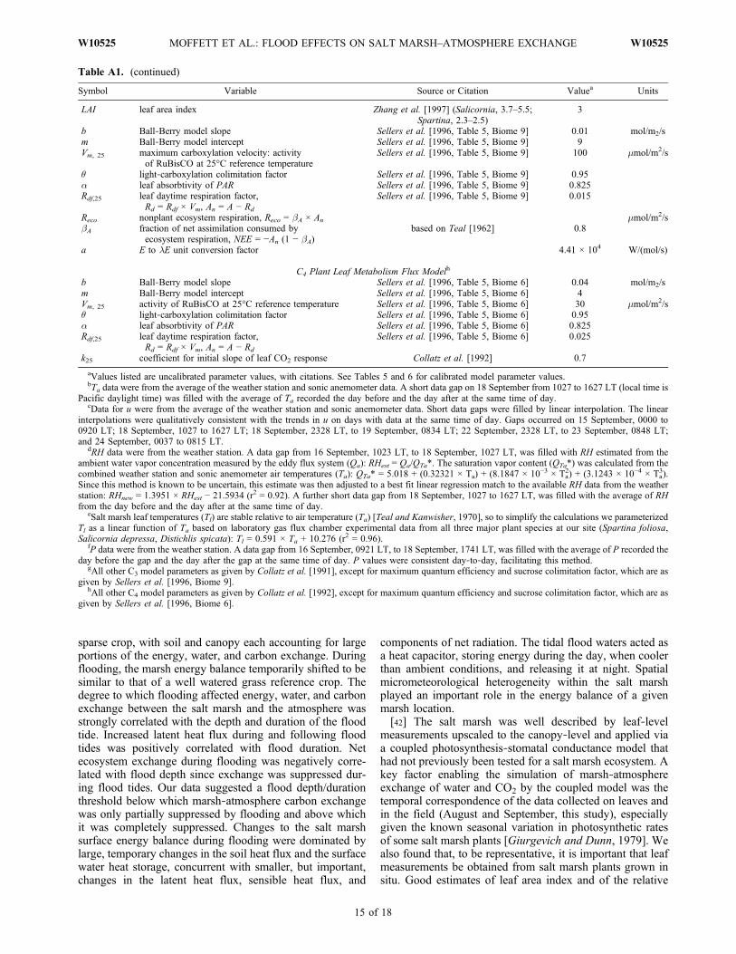
[44] One of the purposes of this study was to evaluate theaccuracy of six common models used to calculate intertidalsalt marsh evapotranspiration with generic “wetland”parameter values from the literature and ambient micro-meteorological data. The six models are summarized inTable 1 of the main text. Such a literature‐based, uncali-brated approach is common in studies seeking to modelsalt marsh hydrology because there have been few datapublished prior to this study that might be used to calibratethe models specifically for salt marshes. Four energy‐driven models are commonly applied in this literature‐based manner, the Priestley‐Taylor, Penman‐Monteith,Wessel‐Rouse (weighted Penman‐Monteith), and pancoefficient models. Biochemical models of C3 and C4 plant

leaf metabolism had not been used to calculate theevapotranspiration of halophytic salt marsh vegetation priorto this study, and so it was especially important to definethe parameters extracted from the literature for use in thesemodels. Table A1 defines the variables in each of the sixmodels and lists the representative “wetland” values fromthe literature used in uncalibrated model calculations. Thefootnotes in Table A1 also specify details of micro-meteorological data processing.

[45] Acknowledgments. This work was supported by the NationalScience Foundation under grant EAR‐0634709 to Stanford University.Any opinions, findings, and conclusions or recommendations expressed inthis material are those of the authors and do not necessarily reflect the viewsof the National Science Foundation. We gratefully acknowledge the City ofPalo Alto Baylands Nature Preserve for their encouragement. We thankC. Field for the use of his field equipment; K. Brauman, R. Pieruschka,and T. Tobeck for help with the equipment; and K. Brauman, L. Erban,S. Vanderhoven, and N. Walker for their field assistance.

ReferencesAllen, R. G., L. S. Pereira, D. Raes, and M. Smith (1998), Crop evapotrans-piration: Guidelines for computing crop water requirements, FAO Irrig.Drain. Pap. 56, Food and Agric. Org., Rome.

Antlfinger, A. E., and E. L. Dunn (1979), Seasonal patterns of CO2 andwater vapor exchange of three salt marsh succulents, Oecologia, 43(3),249–260, doi:10.1007/BF00344952.

Baldocchi, D., and T. Meyers (1998), On using eco‐physiological, micro-meteorological and biogeochemical theory to evaluate carbon dioxide,water vapor and traced gas fluxes over vegetation: A perspective, Agric.For. Meteorol., 90, 1–25, doi:10.1016/S0168-1923(97)00072-5.

Ball, J. T. (1988), An analysis of stomatal conductance, Ph.D. thesis,Stanford Univ., Stanford, Calif.

Bridgham, S. D., J. P. Megonigal, J. K. Keller, N. B. Bliss, and C. Trettin(2006), The carbon balance of north American wetlands,Wetlands, 26(4),889–916, doi:10.1672/0277-5212(2006)26[889:TCBONA]2.0.CO;2.

Broström, A., M. Coe, S. P. Harrison, R. Gallimore, J. E. Kutzbach, J. Foley,I. C. Prentice, and P. Behling (1998), Land surface feedbacks and palaeo-monsoons in northern Africa, Geophys. Res. Lett., 25(19), 3615–3618,doi:10.1029/98GL02804.

Campbell, G. S., and J. M. Norman (1998), An Introduction to Environ-mental Biophysics, 2nd ed., Springer, New York.

Carrington, D. P., R. G. Gallimore, and J. E. Kutzbach (2001), Climatesensitivity to wetlands and wetland vegetation in mid‐Holocene NorthAfrica, Clim. Dyn., 17(2–3), 151–157, doi:10.1007/s003820000099.

Chmura, G. L., S. C. Anisfeld, D. R. Cahoon, and J. C. Lynch (2003),Global carbon sequestration in tidal, saline wetland soils, Global Biogeo-chem. Cycles, 17(4), 1111, doi:10.1029/2002GB001917.

Collatz, G. J., J. T. Ball, C. Grivet, and J. A. Berry (1991), Physiologicaland environmental regulation of stomatal conductance, photosynthesisand transpiration: A model that includes a laminar boundary layer, Agric.For. Meteorol., 54, 107–136, doi:10.1016/0168-1923(91)90002-8.

Collatz, G. J., M. Ribas‐Carbo, and J. A. Berry (1992), Coupled photosyn-thesis‐stomatal conductance model for leaves of C4 plants, Aust. J. PlantPhysiol., 19(5), 519–538, doi:10.1071/PP9920519.

Cornell, J. A., C. Craft, and P. Megonigal (2007), Ecosystem gas exchangeacross a created salt marsh chronosequence, Wetlands, 27(2), 240–250,doi:10.1672/0277-5212(2007)27[240:EGEAAC]2.0.CO;2.

Cornu, C. E., and S. Sadro (2002), Physical and functional responses toexperimental marsh surface elevation manipulation in Coos Bay’s SouthSlough, Restor. Ecol., 10(3), 474–486, doi:10.1046/j.1526-100X.2002.01035.x.

Craft, C., J. Clough, J. Ehman, S. Joye, R. Park, S. Pennings, H. Guo, andM. Machmuller (2009), Forecasting the effects of accelerated sea‐levelrise on tidal marsh ecosystem services, Front. Ecol. Environ., 7(2),73–78, doi:10.1890/070219.

Dacey, J. W. H., and B. L. Howes (1984), Water uptake by roots controlswater table movement and sediment oxidation in short Spartina marsh,Science, 224(4648), 487–489, doi:10.1126/science.224.4648.487.

DeLaune, R. D., S. R. Pezeshki, and W. H. Patrick Jr. (1987), Response ofcoastal plants to increase in submergence and salinity, J. Coastal Res.,3(4), 535–546.

Drake, B. G. (1989), Photosynthesis of salt marsh species, Aquat. Bot., 34,167–180, doi:10.1016/0304-3770(89)90055-7.


16 of 18

Drexler, J. Z., R. L. Snyder, D. Spano, and K. T. Paw U (2004), Areview of models and micrometeorological methods used to estimatewetland evapotranspiration, Hydrol. Processes, 18(11), 2071–2101,doi:10.1002/hyp.1462.

Farquhar, G. D., S. von Caemmerer, and J. A. Berry (1980), A biochemicalmodel of photosynthetic CO2 assimilation in leaves of C3 species,Planta, 149(1), 78–90, doi:10.1007/BF00386231.

Gallagher, J. L. (1983), Seasonal patterns in recoverable undergroundreserves in Spartina alterniflora Loisel, Am. J. Bot., 70(2), 212–215,doi:10.2307/2443265.

Gardner, L. R., and H. W. Reeves (2002), Seasonal patterns in the soilwater balance of a Spartina marsh site at North Inlet, South Carolina,USA, Wetlands, 22(3), 467–477, doi:10.1672/0277-5212(2002)022[0467:SPITSW]2.0.CO;2.

German, E. R. (2000), Regional evaluation of evapotranspiration in theEverglades, Water Res. Invest. Rep. 00‐4217, 48 pp., U.S. Geol. Surv,Reston, Va.

Giurgevich, J. R., and E. L. Dunn (1979), Seasonal patterns of CO2 andwater vapor exchange of the tall and short height forms of Spartinaalterniflora Loisel in a Georgia salt marsh, Oecologia, 43(2), 139–156,doi:10.1007/BF00344767.

Giurgevich, J. R., and E. L. Dunn (1982), Seasonal patterns of daily netphotosynthesis, transpiration and net primary productivity of Juncus roe-merianus and Spartina alterniflora in a Georgia salt marsh, Oecologia,52(3), 404–410, doi:10.1007/BF00367967.

Holmes, R. W., and B. E. Mahall (1982), Preliminary observations on theeffects of flooding and desiccation upon the net photosynthetic rates ofhigh intertidal estuarine sediments, Limnol. Oceanogr., 27(5), 954–958,doi:10.4319/lo.1982.27.5.0954.

Hughes, C. E., J. D. Kalma, P. Binning, G. R. Willgoose, and M. Vertzonis(2001), Estimating evapotranspiration for a temperature salt marsh,Newcastle, Australia, Hydrol. Processes, 15(6), 957–975, doi:10.1002/hyp.189.

Hussey, B. H., and W. E. Odum (1992), Evapotranspiration in tidalmarshes, Estuaries, 15(1), 59–67, doi:10.2307/1352710.

Jiang, L.‐F., Y.‐Q. Luo, J.‐K. Chen, and B. Li (2009), Ecophysiologicalcharacteristics of invasive Spartina alterniflora and native species in saltmarshes of and native species in salt marshes of Yangtze River estuary,China, Estuarine Coastal Shelf Sci., 81(1), 74–82, doi:10.1016/j.ecss.2008.09.018.

Kathilankal, J. C., T. J. Mozdzer, J. D. Fuentes, P. D’Odorico, K. J.McGlathery, and J. C. Zieman (2008), Tidal influences on carbon assim-ilation by a salt marsh, Environ. Res. Lett., 3(4), 044010, doi:10.1088/1748-9326/3/4/044010.

Kirwan, M. L., and G. R. Guntenspergen (2009), Accelerated sea‐level rise—A response to Craft et al., Front. Ecol. Environ, 7(3), 126–127, doi:10.1890/09.WB.005.

Kirwan, M. L., and A. B. Murray (2007), A coupled geomorphic and eco-logical model of tidal marsh evolution, Proc. Natl. Acad. Sci. U. S. A.,104(15), 6118–6122, doi:10.1073/pnas.0700958104.

Knorr, W. (2000), Annual and interannual CO2 exchanges of the terrestrialbiosphere: Process‐based simulations and uncertainties, Glob. Ecol.Biogeogr., 9(3), 225–252, doi:10.1046/j.1365-2699.2000.00159.x.

Krinner, G. (2003), Impact of lakes and wetlands on boreal climate,J. Geophys. Res., 108(D16), 4520, doi:10.1029/2002JD002597.

Kuramoto, R. T., and D. E. Brest (1979), Physiological response to salinityby four salt marsh plants, Bot. Gaz., 140(3), 295–298, doi:10.1086/337089.

Lafleur, P. M. (2008), Connecting atmosphere and wetland: Energy andwater vapour exchange, Geogr. Compass, 2(4), 1027–1057, doi:10.1111/j.1749-8198.2007.00132.x.

Lana, P. C., C. Guiss, and S. T. Disaró (1991), Seasonal variation ofbiomass and production dynamics for above‐ and belowground com-ponents of a Spartina alterniflora marsh in the euhaline sector ofParanaguá Bay (SE Brazil), Estuarine Coastal Shelf Sci., 32(3),231–241, doi:10.1016/0272-7714(91)90017-6.

Li, H., L. Li, and D. Lockington (2005), Aeration for plant root respira-tion in a tidal marsh, Water Resour. Res., 41, W06023, doi:10.1029/2004WR003759.

Linthurst, R. A., and E. D. Seneca (1980), The effects of standing water anddrainage potential on the Spartina alterniflora‐substrate complex in aNorth Carolina salt marsh, Estuarine Coastal Mar. Sci., 11(1), 41–52,doi:10.1016/S0302-3524(80)80028-4.

Magenheimer, J. F., T. R. Moore, G. L. Chmura, and R. J. Daoust (1996),Methane and carbon dioxide flux from a macrotidal salt marsh, Bay of

Fundy, New Brunswick, Estuaries, 19(1), 139–145, doi:10.2307/1352658.

Marani, M., A. D’Alpaos, S. Lanzoni, L. Carniello, and A. Rinaldo (2007),Biologically controlled multiple equilibria of tidal landforms and the fateof the Venice lagoon, Geophys. Res. Lett., 34, L11402, doi:10.1029/2007GL030178.

Miller, W. D., S. C. Neubauer, and I. C. Anderson (2001), Effects of sealevel induced disturbances on high salt marsh metabolism, Estuaries,24(3), 357–367, doi:10.2307/1353238.

Monteith, J. L. (1965), Evaporation and environment, Symp. Soc. Exp.Biol., 19, 205–224.

Morris, J. T. (1995), The mass balance of salt and water in intertidalsediments: Results from North Inlet, South Carolina, Estuaries, 18(4),556–567, doi:10.2307/1352376.

Morris, J. T., P. V. Sundareshwar, C. T. Nietch, B. Kjerfve, and D. R.Cahoon (2002), Responses of coastal wetlands to rising sea level,Ecology, 83(10), 2869–2877, doi:10.1890/0012-9658(2002)083[2869:ROCWTR]2.0.CO;2.

Nicholls, R. J. (2004), Coastal flooding and wetland floss in the 21st century:Changes under the SRES climate and socio‐economic scenarios, Glob.Environ. Change, 14(1), 69–86, doi:10.1016/j.gloenvcha.2003.10.007.

Nyman, J. A., and R. D. DeLaune (1991), CO2 emission and soil Ehresponses to different hydrological conditions in fresh, brackish, andsaline marsh soils, Limnol. Oceanogr., 36(7), 1406–1414, doi:10.4319/lo.1991.36.7.1406.

Pearcy, R. W., and S. L. Ustin (1984), Effects of salinity on growth andphotosynthesis of three California tidal marsh species, Oecologia, 62(1),68–73, doi:10.1007/BF00377375.

Pezeshki, S. R. (2001), Wetland plant responses to soil flooding, Environ.Exp. Bot., 46(3), 299–312, doi:10.1016/S0098-8472(01)00107-1.

Priestley, C. H. B., and R. J. Taylor (1972), On the assessment of surfaceheat flux and evaporation using large‐scale parameters, Mon. WeatherRev., 100(2), 81–92, doi:10.1175/1520-0493(1972)100<0081:OTAOSH>2.3.CO;2.

Rosso, P. H., S. L. Ustin, and A. Hastings (2006), Use of lidar to studychanges associated with Spartina invasion in San Francisco Baymarshes, Remote Sens. Environ., 100(3), 295–306, doi:10.1016/j.rse.2005.10.012.

Schemel, L. E., R. L. Brown, and N. W. Bell (2003), Salinity and tem-perature in south San Francisco Bay, California at Dumbarton Bridge:Results from the 1999–2002 water years and an overview of previousdata, Water Res. Invest. Rep. 03‐4005, 32 pp., U.S. Geol. Surv, MenloPark, Calif.

Sellers, P. J., S. O. Los, C. J. Tucker, C. O. Justice, D. A. Dazlich, G. J.Collatz, and D. A. Randall (1996), A revised land surface parameteriza-tion (SiB2) for atmospheric GCMs. Part II: The generation of globalfields of terrestrial biophysical parameters from satellite data, J. Clim.,9(4), 706–737, doi:10.1175/1520-0442(1996)009<0706:ARLSPF>2.0.CO;2.

Shuttleworth, W. J. (1993), Evaporation, in Handbook of Hydrology, editedby D. R. Maidment, chap. 4, pp. 4.1–4.53, McGraw‐Hill, New York.

Shuttleworth, W. J., and J. S. Wallace (1985), Evaporation from sparsecrops—An energy combination theory, Q. J. R. Meteorol. Soc., 111(469),839–855.

Simas, T. C., and J. G. Ferreira (2007), Nutrient enrichment and the role ofsalt marshes in the Tagus estuary (Portugal), Estuarine Coastal ShelfSci., 75(3), 393–407, doi:10.1016/j.ecss.2007.05.046.

Steinke, W., D. J. von Willert, and F. A. Austenfeld (1996), Root dynamicsin a salt marsh over three consecutive years, Plant Soil, 185(2), 265–269,doi:10.1007/BF02257532.

Teal, J. M. (1962), Energy flow in the salt marsh ecosystem of Georgia,Ecology, 43(4), 614–624, doi:10.2307/1933451.

Teal, J. M., and B. L. Howes (1996), Interannual variability of a salt‐marshecosystem, Limnol. Oceanogr., 41(4), 802–809, doi:10.4319/lo.1996.41.4.0802.

Teal, J. M., and J. Kanwisher (1970), Total energy balance in salt marshgrasses, Ecology, 51(4), 690–695, doi:10.2307/1934050.

Tol, R. S. J. (2007), The double trade‐off between adaptation and mitiga-tion for sea level rise: An application of FUND, Mitigation Adapt. Strat-egies Global Change, 12(5), 741–753, doi:10.1007/s11027-007-9097-2.

Twine, T. E., W. P. Kustas, J. M. Norman, D. R. Cook, P. R. Houser, T. P.Meyers, J. H. Prueger, P. J. Starks, and M. L. Wesely (2000), Correctingeddy‐covariance flux underestimates over a grassland, Agric. For.Meteorol., 103(3), 279–300, doi:10.1016/S0168-1923(00)00123-4.


17 of 18

Ursino, N., S. Silvestri, and M. Marani (2004), Subsurface flow and vege-tation patterns in tidal environments, Water Resour. Res., 40, W05115,doi:10.1029/2003WR002702.

Valiela, I., J. M. Teal, and N. Y. Persson (1976), Production and dynamicsof experimentally enriched salt marsh vegetation: Belowground biomass,Limnol. Oceanogr., 21(2), 245–252, doi:10.4319/lo.1976.21.2.0245.

Wessel, D. A., and W. R. Rouse (1994), Modeling evaporation from wet-land tundra, Boundary Layer Meteorol., 68(1–2), 109–130, doi:10.1007/BF00712666.

Wigand, C., P. Brennan, M. Stolt, M. Holt, and S. Ryba (2009), Soil res-piration rates in coastal marshes subject to increasing watershed nitrogenloads in southern New England, USA, Wetlands, 29(3), 952–963,doi:10.1672/08-147.1.

Wolf, A., K. Akshalov, N. Saliendra, D. A. Johnson, and E. A. Laca(2006), Inverse estimation of Vcmax, leaf area index, and the Ball‐Berry

parameter from carbon and energy fluxes, J. Geophys. Res., 111,D08S08, doi:10.1029/2005JD005927.

Zhang, M., S. L. Ustin, E. Rejmankova, and E. W. Sanderson (1997), Mon-itoring Pacific coast salt marshes using remote sensing, Ecol. Appl., 7(3),1039–1053, doi:10.1890/1051-0761(1997)007[1039:MPCSMU]2.0.CO;2.

J. A. Berry and A. Wolf, Department of Global Ecology, CarnegieInstitution for Science, 260 Panama St., Stanford, CA 94305, USA.S. M. Gorelick and K. B. Moffett, Department of Environmental Earth

System Science, Stanford University, Y2E2 Bldg., MC 4216, 473 ViaOrtega, Stanford, CA 94305, USA. ([email protected])


18 of 18

salt marsh atmosphere exchange of energy, water … climate with winter precipitation (october to...

Documents