SAMPLE SELECTION

Cheti NicolettiISER, University of Essex

2009

Wage equation and labour participation for women

Gourieroux C. (2000),  Econometrics of Qualitative Dependent Variables, Cambridge University Press, Cambridge

• Let y* be the potential offered wage and let w be the reservation wage then the observed wage y is given by

• Let us consider the following very simple earnings profile equation

wy

wyyy

*

**

if 0

if

agey 10

*

not work does woman a i.e.if 0

k woman wora i.e. if1*

*

wy

wyd

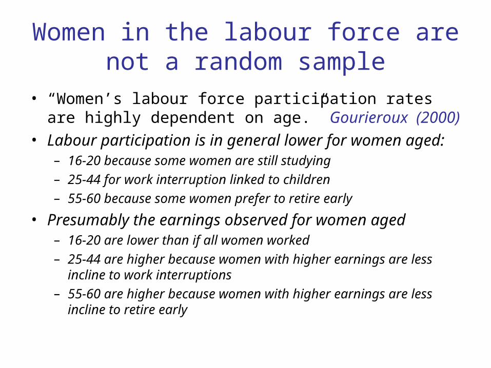
Women in the labour force are not a random sample

• “Women’s labour force participation rates are highly dependent on age.” Gourieroux (2000)

• Labour participation is in general lower for women aged:– 16-20 because some women are still studying– 25-44 for work interruption linked to children– 55-60 because some women prefer to retire early

• Presumably the earnings observed for women aged– 16-20 are lower than if all women worked– 25-44 are higher because women with higher earnings are less

incline to work interruptions – 55-60 are higher because women with higher earnings are less

incline to retire early

Women career profile

0

1000

2000

3000

4000

5000

0 20 40 60 80

age

ea

rnin

gs

Sample selection model Labour participation equation

• Probit model for labour participation

)()|1Pr(

)1,0(*

zzd

Niiduwhereuzd

not work does woman a if 0

k woman wora if1d

n

i

d

i

d

iii zzL

1

11

work topropensity theis * where d

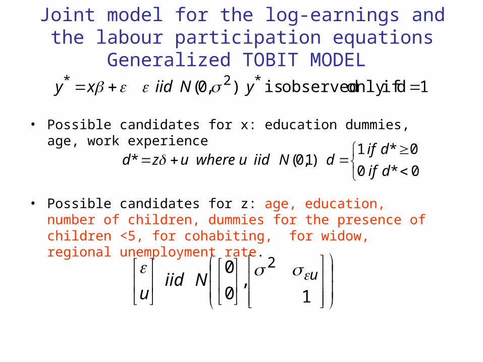
Joint model for the log-earnings and the labour participation equations

Generalized TOBIT MODEL

• Possible candidates for x: education dummies, age, work experience

• Possible candidates for z: age, education, number of children, dummies for the presence of children <5, for cohabiting, for widow, regional unemployment rate.

0*0

0*1)1,0(*

dif

difdNiiduwhereuzd

1d ifonly observed is ),0( *2* yNiidxy

1,

0

0 2uNiid

u

22

1221

2

1

2

1 ,isIf

m

mN

y

y

),(isThen 2111 mNy

)/,/)((is|and 21

212

22

211112212 mymNyy

1,

0

0isIf

2uN

u

)1,0(isThen Nv ),(is|and 22uuuNu

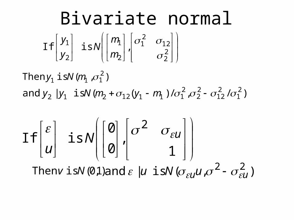
Bivariate normal

Truncated Normal

Suggestions for the proof

)1,0(~ NY

Z

c and ratio) sMill' (inverse

1 where

c

cY then Z If

zzzzzzzzdz

zzdzz

dz

zd)()()()()(

)( and )(

)( 22

Normal Truncated~ then ),(~ If 2 cYYNY

22 1c)YVar(Y and c)YE(Ywith

Sample selection problem

E(y*|d=1,x,z)=x+E(|d=1,x,z)

E(|d=1,x,z)= E(|u>-zδ )=

E(y*|d=1,x,z)= X

)(

)()|(

z

zzuuE uu

)(

)(

z

zu

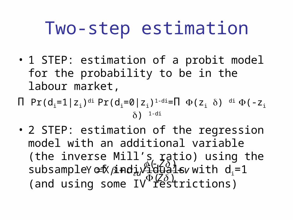
Two-step estimation

• 1 STEP: estimation of a probit model for the probability to be in the labour market,

Π Pr(di=1|zi)di Pr(di=0|zi)1-di=Π (zi ) di (-zi ) 1-di

• 2 STEP: estimation of the regression model with an additional variable (the inverse Mill’s ratio) using the subsample of individuals with di=1 (and using some IV restrictions)

vZ

Zu

)(

)( XY

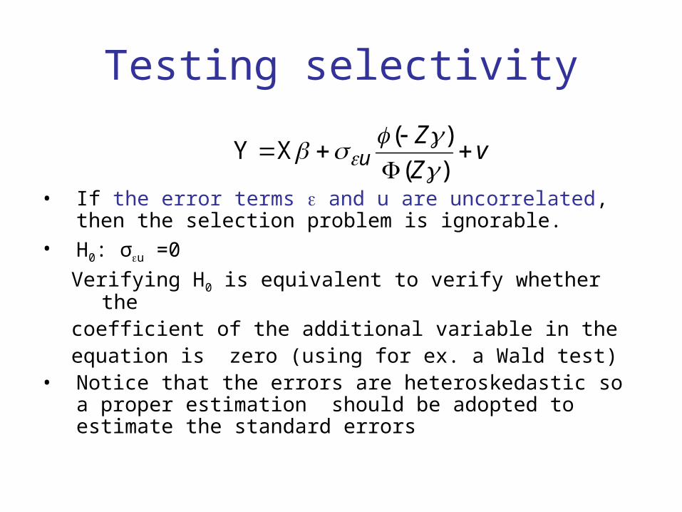
Testing selectivity

• If the error terms and u are uncorrelated, then the selection problem is ignorable.

• H0: σu =0

Verifying H0 is equivalent to verify whether the coefficient of the additional variable in the equation is zero (using for ex. a Wald test)

• Notice that the errors are heteroskedastic so a proper estimation should be adopted to estimate the standard errors

vZ

Zu

)(

)( XY

Generalized Tobit: Maximum Likelihood Estimation

xy* uzd *

1,

0

0 2uNiid

v

1,

,|

,| 2

*

*u

z

xNiid

zxd

zxy

2* ,| xNiidxy

2

2*

2** 1,,,|

uu xyzNiidzxyd

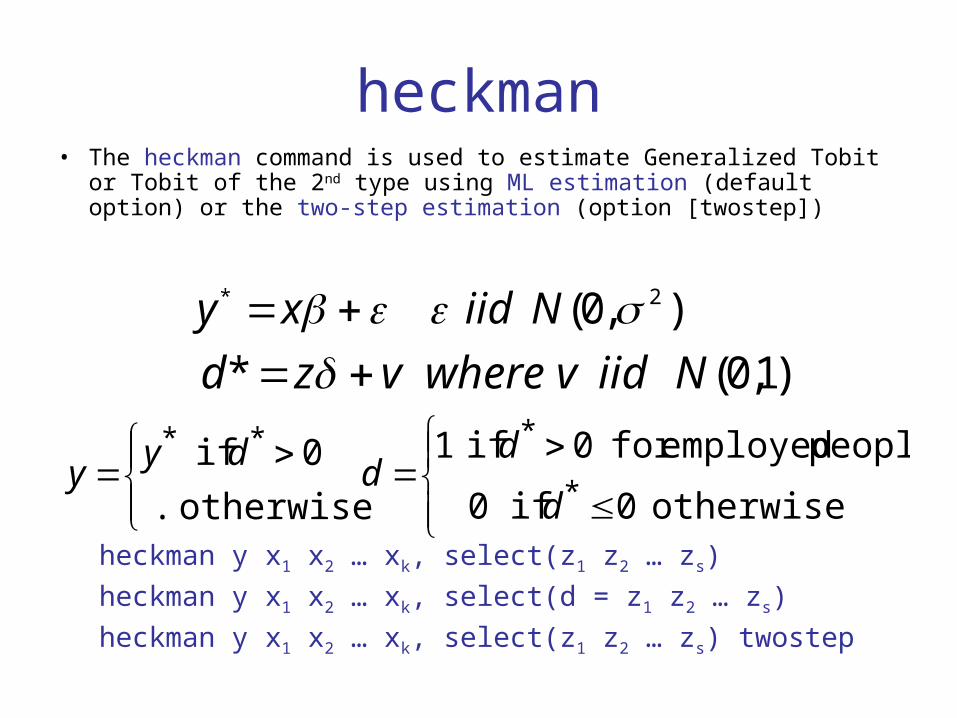
heckman• The heckman command is used to estimate Generalized Tobit or

Tobit of the 2nd type using ML estimation (default option) or the two-step estimation (option [twostep])

heckman y x1 x2 … xk, select(z1 z2 … zs)

heckman y x1 x2 … xk, select(d = z1 z2 … zs)

heckman y x1 x2 … xk, select(z1 z2 … zs) twostep

),0( 2* Niidxy )1,0(* Niidvwherevzd

otherwise0if 0

people employedfor 0if1

otherwise .

0if*

***

d

dd

dyy

Generalized Tobit: Maximum Likelihood Estimation

iiii

xyxyf

** 1

)(

n

i

d

iiiii

d

ii

ii yzdxyfzdL1

***1* ),0Pr()()0Pr(

iiiii zvzzd )0Pr()0Pr( *

2

2*

2** 1,,,|

uii

uiiiii xyzNiidzxyd

2

2*

2

*2

*2

***

1

Pr),,0Pr(

uui

iiu

iiiu

iiiiii

xyz

xyzxyzdxzyd

Joint model Two-step estimation

Variable Coeff p-value Coeff p-value

LABOUR PARTICIPATION MODEL

Constant -0.57 0.06 -0.99 0.04

No. children <18 -0.12 0.00 -0.13 0.00

No. children <4 -0.09 0.00 -0.07 0.00

log husband's wage -0.10 0.04 -0.08 0.06

Years of education 0.15 0.00 0.14 0.00

Age 0.81 0.01 0.91 0.02

Age square -0.12 0.03 -0.14 0.01

Correlation between error 0.35 0.00

Inverse Mill's ration 0.29 0.00

WAGE MODEL

Constant 4.50 0.02 4.70 0.01

Years of education 0.11 0.01 0.10 0.00

Work experience 0.13 0.01 0.08 0.01

Work experience square 0.00 0.02 0.01 0.00

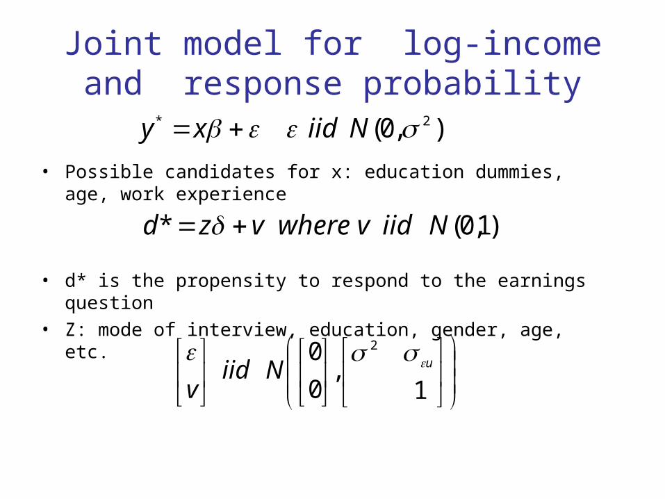
Joint model for log-income and response probability

• Possible candidates for x: education dummies, age, work experience

• d* is the propensity to respond to the earnings question • Z: mode of interview, education, gender, age, etc.

)1,0(* Niidvwherevzd

),0( 2* Niidxy

1

,0

0 2

uNiidv

Item nonresponse for income equation or poverty model in cross section

sample surveys:

Potential explanatory variables:• Socio-demographic variables: age, gender, level

of education, number of adults, number of children.

• Situational economic circumstance: labour status activity.

• Data collection characteristics: mode of the interview, number of visits, duration of the interview. (These are plausible IV)

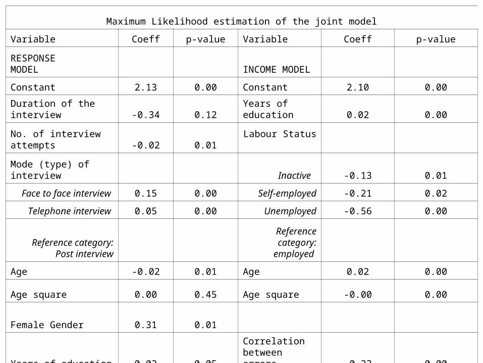
Maximum Likelihood estimation of the joint model

Variable Coeff p-value Variable Coeff p-value

RESPONSE MODEL INCOME MODEL

Constant 2.13 0.00 Constant 2.10 0.00

Duration of the interview -0.34 0.12 Years of education 0.02 0.00

No. of interview attempts -0.02 0.01 Labour Status

Mode (type) of interview Inactive -0.13 0.01

Face to face interview 0.15 0.00 Self-employed -0.21 0.02

Telephone interview 0.05 0.00 Unemployed -0.56 0.00

Reference category: Post interview

Reference category: employed

Age -0.02 0.01 Age 0.02 0.00

Age square 0.00 0.45 Age square -0.00 0.00

Female Gender 0.31 0.01  

Years of education 0.02 0.05Correlation between errors -0.23 0.00

Attrition in panel surveys has two possible causes: failed contact and refusal

The potential variables explaining attrition (contact and cooperation) are lagged variables observed in the last wave.

The equation of interest has to use lagged variables (otherwise we have missing explanatory variables too)

• Socio-demographic variables: age, gender, level of education, number of adults, number of children.

• Social-integration: talking often to neighbours, cohabitation, house ownership.

• Situational economic circumstance: labour status activity, household equalised income.

• Data collection characteristics: mode of the interview, number of visits, duration of the interview, same interviewer across wave, duration of the panel, length of the fieldwork. (These are plausible IV)

Attrition due to lack of cooperation (BHPS 1994-96) Variables Coefficients Test p-value

Wave 1996 0.17108 2.21 0.027

Workload -0.01619 -22.04 0.000

Item nonresponse by interviewer -3.08725 -3.74 0.000

Co-operation rate by interviewer 1.62772 4.85 0.000

Age 35 or less -0.05109 -0.58 0.560

Age 60 or more -0.01904 -0.15 0.882

Female 0.20994 2.77 0.006

Living without a spouse -0.15878 -1.90 0.057

No. of children -0.03666 -0.96 0.337

No. of adults -0.06812 -1.68 0.092

Unemployed -0.38718 -3.00 0.003

Inactive 0.16281 1.64 0.100

No. of visits -0.02887 -2.33 0.020

Same interviewer 0.61158 7.78 0.000

Item nonresponse 0.04194 0.20 0.843

Constant 1.54751 7.30 0.000

Wald joint significance test 2068.9 No. obs. 14265

Weighted estimation),0( 2* Niidxy

)1,0(* Niidvwherevzd

missing is if0if 0

observed is if 0if1

otherwise .

0if**

****

yd

ydd

dyy

)()|1Pr()|0*Pr(

of inverse by thegiven are Weights

zzdzd

variablesobservedgiven d oft independen *y

:(MAR) randomat missing of Assumption

Weighted estimation

),0( 2* Niidxy

consistent is estimation squaresleast weighted that theso

0)|)('[

that provecan then we),(given oft independen is If

0)|)('[

onlyconsider can but we

0)|)('[on based is OLS

1*

*

*

*

xdxyxE

zxyd

xdxyxE

xxyxE

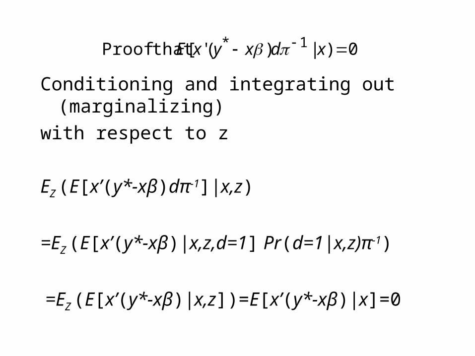
Conditioning and integrating out (marginalizing)

with respect to z

EZ (E[x’(y*-xβ)dπ-1]|x,z)

=EZ (E[x’(y*-xβ)|x,z,d=1] Pr(d=1|x,z)π-1)

=EZ (E[x’(y*-xβ)|x,z])=E[x’(y*-xβ)|x]=0

0)|)('[ that Proof 1* xdxyxE

How to use weights in Stata• Most Stata commands can deal with weighted data. Stata

allows four kinds of weights:1. fweights, or frequency weights, are weights that

indicate the number of duplicated observations.2.pweights, or sampling weights, are weights that

denote the inverse of the probability that the observation is included due to the sampling design, nonresponse or sample selection.

3.aweights, or analytic weights, are weights that are inversely proportional to the variance of an observation; i.e., the variance of the j-th observation is assumed to be sigma^2/w_j, where w_j are the weights.

4. iweights, or importance weights, are weights that indicate the "importance" of the observation in some vague sense.

Option pweights• Usually sample surveys provide weights to take account of sampling

design, nonresponse . • Let p be individual weight• Then we can run a regression with weighted observationsregress y x1 x2 … xk [pweight=p]

• Let us assume to have a random sample affected by nonresponse, but weights to take account of unit nonresponse are not available

• A possible way to estimate your own weights is described in the following:

probit d z1 z2 … zs

predict propgen invprop=1/propreg y x1 x2 … xk [pweight=invprop]

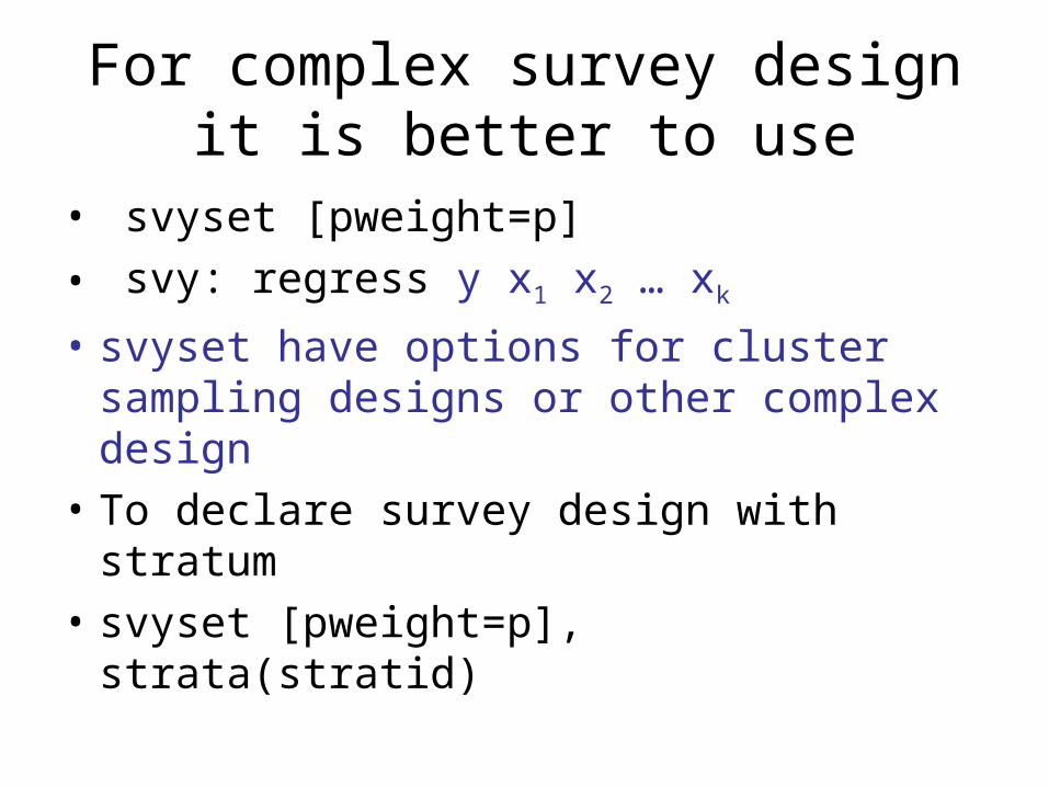
For complex survey design it is better to use

• svyset [pweight=p]

• svy: regress y x1 x2 … xk

• svyset have options for cluster sampling designs or other complex design

• To declare survey design with stratum

• svyset [pweight=p], strata(stratid)

Stata propensity score methods for evaluation of treatment

Abadie A., Drukker D., Herr J.L., Imbens G.W. (2001), Implementing Matching Estimators for Average Treatment Effects in Stata, The Stata Journal, 1, 1-18 http://ksghome.harvard.edu/~.aabadie.academic.ksg/software.html

Becker S.O., Ichino A. (2002), Estimation of average treatment effects based on propensity scores. The Stata Journal, 2, 358-377 http://www.lrz-muenchen.de/~sobecker/pscore.html

Sianesi B. (2001), Implementing Propensity Score Matching Estimators with STATA, UK Stata Users Group, VII Meeting London, http://ideas.repec.org/c/boc/bocode/s432001.html

Some references for regressions with sample selection

• Buchinski, M. (2001) Quantile regression with sample selection: Estimation women return to education in the U.S., Empirical Economics, 26, 86-113.

• Ibrahim, J.G., Chen, M.-H., Lipsitz, S.R., Herring, A.H. (2005) Missing-data methods for generalized linear models: A comparative review, Journal of the American Statistical Association, 100, 469, 332-346.

• Lipsitz, S.R., Fitzmaurice, G.M., Molenberghs, G., Zhao, L.P. (1997), Quantile regression methods for longitudinal data with drop-outs, Applied Statistics, 46, 463-476.

• Robins, J. M., Rotnitzky, A. (1995), Semiparametric Effciency in Multivariate Regression Models With Missing Data, Journal of the American Statistical Association, 90, 122-129.

• Vella F. (1998), Estimating models with sample selection bias: a survey', The Journal of Human Resources, vol. 3, 127-169.

• Wooldridge, J.M. (2007) Inverse probability weighted M-Estimation for General missing data problems, Journal of Econometrics, 141, 2, 1281-1301.

• Wooldridge, J.M. (2007) Inverse probability weighted M-Estimation for General missing data problems, Journal of Econometrics, 141, 2, 1281-1301.