sampling design used in the national motor vehicle crash

Sampling Design Used in the National Motor Vehicle Crash Causation Survey

DOT HS 810 930 April 2008

Technical Report

Published By:NHTSA’s National Center for Statistics and Analysis

This report is free of charge from the NHTSA Web site at www.nhtsa.dot.gov This document is available to the public from the National Technical Information Service, Springfield, Virginia 22161

This publication is distributed by the U.S. Department of Transportation, National Highway Traffic Safety Administration, in the interest of information exchange. The opinions, findings and conclusions expressed in this publication are those of the author(s) and not necessarily those of the Department of Transportation or the National Highway Traffic Safety Administration. The United States Government assumes no liability for its content or use thereof. If trade or manufacturer’s names or products are mentioned, it is because they are considered essential to the object of the publication and should not be construed as an endorsement. The United States Government does not endorse products or manufacturers.

Technical Report Documentation Page 1. Report No.

DOT HS 810 930 2. Government Accession No.

3. Recipients's

Catalog No.

4. Title and Subtitle

Sampling Design Used in

Causation Survey

the National Motor Vehicle Crash

5. Report Date

April 2008 6. Performing Organization Code

NVS-421

7. Author(s)

Eun-Ha Choi, Fan Zhang, Eun Young Noh, Santokh Singh, and

Chou-Lin Chen

8. Performing Organization Report No.

9. Performing Organization Name and Address

National Center for Statistics and Analysis

National Highway Traffic Safety Administration

U.S. Department of Transportation

1200 New Jersey Avenue SE.

Washington, DC 20590

10.

Work Unit No. (TRAIS)n code

11. Contract of Grant No.

12. Sponsoring Agency Name and Address

National Center for Statistics and Analysis

National Highway Traffic Safety Administration

U.S. Department of Transportation

1200 New Jersey Avenue SE.

Washington, DC 20590

13. Type of Report and Period Covered

NHTSA Technical Report

14. Sponsoring Agency Code

15.Supplementary Notes

Selection of crashes through NMVCCS ceased on December 31, 2007.

This paper was originally presented at the Transportation Research Board 87th Annual Meeting, held

Fan Zhang is a mathematical statistician in National Science Foundation.

in Washington, DC, January 13-17, 2008.

16. Abstract

The purpose of the National Motor Vehicle Crash Causation Survey (NMVCCS) was to collect information on the vehicles, the

roadways, and the environmental conditions as well as the human behavioral factors that are likely to contribute to crash

occurrence. The data was collected on crashes involving light vehicles, during the period January 2005 to December 2007. The

primary focus of the survey is on the events immediately prior to a crash as well as on the associated factors as described by the

occupants and witnesses, reported by the police, and assessed by the NMVCCS researchers. One of the special features of

NMVCCS was to collect information at the crash scene itself, thus enabling the researcher to obtain first-hand information while it

was still relatively undisturbed. Due to the nature of the targeted information and the method of operation, this survey required a

complex sample design to get national representation at a reasonable cost. Both time and location of a crash were considered in the

selection of crashes to attain high efficiency of the on-scene survey.

A two-dimensional sampling frame reflecting on both space and time of crash occurrence was used in sampling crashes from

among those occurring between 6 a.m. and midnight. A probability-based sampling procedure was performed in multiple stages. In

order to make the NMVCCS sample nationally representative, the inclusion probability in each sampling stage was taken into

account in developing the weights. While doing so, appropriate adjustments were made for the crashes from which information

could not be collected due to the operational difficulties and other challenges. This report provides details of the sampling

procedure and the related operational challenges. The analytical details of the estimation methodology are also discussed. Some

national estimates and their standard errors, based on the data collected during the first year of its operation, are presented.

17. Key Words

Crash causation, on-scene, sample design, multi-stage sampling,

weight

18. Distribution Statement

This report is free of charge from the NHTSA

www.nhtsa.dot.gov

Web site at

19.

Security Classif. (of this report)

Unclassified

20.

Security Classif. (of this page)

Unclassified

21. No of Pages

23

22. Price

Form DOT F1700.7 (8-72) Reproduction of completed page authorized

Table of Contents

1. Executive Summary ............................................................................................. 1

2. Introduction.......................................................................................................... 3

3. Objective of the Sample Design ........................................................................... 3

4. Target Population ................................................................................................ 4

5. Sampling Frame ................................................................................................... 4

6. Sample Size........................................................................................................... 6

7. Data Collection Methodology .............................................................................. 6

8. Sampling Procedure............................................................................................. 6

8.1. First Stage: Selection of PSU .................................................................... 7

8.2. Second Stage: Selection of a Sub-Sampling Unit in Certain PSUs............. 7

8.3. Third Stage: Selection of a Time Strip....................................................... 8

8.4. Fourth State: Selection of Days of Week ................................................... 9

8.5. Fifth Stage: Selection of a Crash in the Selected Time Blocks ..................10

8.6. Time Block Reduction .............................................................................11

9. Estimation Procedure .........................................................................................12

9.1. Design Weight..........................................................................................12

9.2. Adjustment of Design Weight for Time Blocks With a Missing Crash ......12

9.2.1. Adjustment at Week Level.....................................................13

9.2.2. Adjustment at PSU Level.......................................................14

10. Some Highlights of NMVCCS ............................................................................15

10.1. Sampling Statistics..................................................................................15

10.2. Estimation...............................................................................................16

11. References............................................................................................................18

1. Executive Summary

NHTSA’s National Center for Statistics and Analysis, 1200 New Jersey Avenue SE., Washington, DC 20590

1

The purpose of the National Motor Vehicle Crash Causation Survey (NMVCCS) was to collect

information on the vehicles, roadways, environmental conditions, and human behavioral factors

that are likely to contribute to crash occurrence. The data was collected on crashes involving

light vehicles during the period January 2005 to December 2007. The primary focus is on the

events that occurred immediately prior to each crash, as well as on the associated factors. Due to

the nature of the targeted information and the operational complexity of investigating a crash at

the crash scene, NMVCCS used a complex, probability-based sample design to achieve national

representation at a reasonable cost. This report provides details about the sample design used for

this survey.

The population of interest in NMVCCS consists of crashes that resulted in a harmful event

involving at least one light vehicle with a gross vehicle weight (GVW) less than 10,000 pounds

that was towed due to damage. However, due to operational challenges resulting from on-scene

requirements of the survey and other constraints, the target population was restricted to crashes

occurring between 6 a.m. and midnight that also had a completed police accident report and to

which emergency medical services (EMS) had been dispatched.

Due to the random nature of crash occurrence with respect to the location and time, there was no

existing sampling frame available in advance for selection of a sample of crashes from the

population of interest. Taking into account these facts, a two-dimensional sampling frame

reflecting on both the location and the time of crash occurrence was used in sampling crashes

from among those occurring between 6 a.m. and midnight.

In the absence of existing sampling frame in advance and due to the inherent uncertainty in the

rate of a successful crash investigation in a sampled time interval, the sample size was

determined based on practical considerations rather than the magnitude of sampling errors. As a

result, two researchers were assigned to each of the 24 pre-determined geographic locations and

each researcher was required to investigate at most two crashes per week. Taking these

operational arrangements and adjustments into consideration, NMVCCS targeted to sample

about 5,000 crashes per year.

Regarding the operation of the survey, the researchers monitored the EMS radio frequencies (or

the police notifications in certain primary sampling units [PSUs]) to arrive at the crash scene in a

timely manner. Upon arriving at the crash scene, they made a determination as to whether the

crash qualified for NMVCCS investigation. An investigation of the crash was initiated after a

positive determination of the required criteria for qualification. The information was then

collected from all available sources using a set of forms and a portable computer.

The selection of crashes in NMVCCS was accomplished through a multistage sampling

procedure. At each stage, samples were drawn with unequal probability based on the number of

crashes that occurred in a sampling unit, as estimated from the number of crashes coded in the

National Automotive Sampling System (NASS) – Crashworthiness Data System (CDS) in the

previous year. This gave a larger sampling unit a greater chance of being selected in the sample.

Specifically, the NMVCCS sampling procedure consists of the following five stages:

First Stage: Selection of PSU (geographical area as defined in NASS);

Second Stage: Selection of a sub-sampling unit (defined by EMS agencies, police

jurisdictions, police radio frequencies or geographic areas depending upon the nature of

issues) in a certain PSU, as necessary;

Third Stage: Selection of a time strip (a six-hour time interval between 6 a.m. and

midnight) for each of the selected PSUs;

Fourth Stage: Selection of days of the week for the selected time strip;

Fifth Stage: Selection of a crash within the selected time block, the combination of the

selected day of the week and the time strip.

A comprehensive weighting procedure, that makes the NMVCCS sample nationally

representative, consists of mainly two phases, the design weight and its appropriate adjustment.

The design weight is calculated by taking the reciprocal of the probability of inclusion

of a crash, which is the product of the sampling probabilities at all stages of the

sampling procedure.

The design weights are further adjusted to compensate for the crashes that were missed

due to operational issues. As a result, the design weights of time blocks with missing

crashes are distributed to other time blocks that have a sampled crash.

During the data collection period from July 2005 to June 2006, a total of 2,113 crashes were

sampled from the 24 PSUs through a multistage sampling procedure and were fully investigated

for NMVCCS database. Weights have been assigned to these crashes by using the estimation

procedure described above. The assigned weights have a right-skewed distribution with a

minimum weight of 6.2, a median weight of 216, and a maximum weight of 6,402. Also, about

50 percent of the sampled crashes have their weights between 100 and 400, and 90 percent

between 40 and 1,320.

As examples, some national estimates and their standard errors are presented in this report to

demonstrate the performance of NMVCCS according to the sampling design implemented in this

survey. The following statistics are based on a subset of the all the data collected through

NMVCCS and hence caution should be exercised in interpreting these estimates. They are

merely provided to give an idea of the estimation procedure as well as the nature of data

collected. Based on the weights assigned to crashes, at the national level, the 2,113 sampled

crashes are representative of 807,738 crashes during the period from July 2005 to June 2006. Of

the estimated 807,738 crashes, about 58 percent (with standard error 2.5 percent) were two-

vehicle crashes, about 31 percent (with standard error 2.7 percent) were single-vehicle crashes,

and about 11 percent (with standard error 0.6 percent) involved three or more vehicles. In about

40 percent (with standard error 2.2 percent) of the crashes in which critical reasons were

attributed to the drivers, the critical reason was recognition errors. Among other critical reasons,

the decision errors were assigned in about 37 percent (with standard error 2.2 percent), the

performance error in about 10 percent, and the non-performance errors in about 7.8 percent of

such crashes.


2


3

2. Introduction

The traffic safety community has made great strides in the crashworthiness of vehicles – the

ability of vehicles to protect their occupants in a crash. To substantially reduce the high number

of traffic fatalities and injuries, more needs to be done in primary prevention, i.e., finding ways

to prevent crashes by understanding the events leading up to a crash. Currently available

databases, such as the NASS–CDS at NHTSA do not provide sufficient information that can

specifically serve this purpose. In fact, based on the police accident reports, the crash

investigation in CDS is initiated days or even weeks later and hence does not have enough

potential to reliably identify pre-crash scenarios, critical pre-crash events, and the reason

underlying the critical pre-crash events. Additional data is needed to identify these crash

elements that are crucial for the development of crash avoidance countermeasures, as well as

evaluation and development of emerging crash avoidance technologies.

With this objective, in 2005 NHTSA’s National Center for Statistics and Analysis (NCSA)

started conducting NMVCCS on the lines of the Indiana Tri-Level Study conducted in 1979 and

the Large-Truck Crash Causation Study conducted in 2004. Like these two studies, NMVCCS

collected on-scene information pertaining to pre-crash events and the factors contributing to

crash occurrence, though the targeted crashes in NMVCCS were restricted to the ones that

involved at least one towed light vehicle such as a passenger car, van, sport utility vehicle, or

light truck. The information was collected from all available sources: the crash scene, police,

vehicles, drivers or their surrogates, as well as witnesses, through interviews. The information

thus collected can be used in both statistical analysis and clinical studies to gain more insight into

the motor vehicle crash causation on U.S. highways.

This paper provides details about the sampling procedure used in obtaining the NMVCCS

targeted information as well as the estimation procedure. The objective of the sample design and

details of the target population are described in sections 3 and 4, respectively. The discussion on

the sampling frame and the sample size is included in sections 5 and 6. Data collection

methodology is briefly described in section 7. Section 8 provides details of the multistage

sampling procedure employed in this survey. This section also discusses how the operational

challenges were met. In section 9, the estimation procedure is explained with the analytical and

statistical details of the formulas for calculating weights. In section 10 some statistics are

presented to illustrate the performance of the sampling and estimation procedures used in

NMVCCS. The last section provides a list of references used in this report.

3. Objective of the Sampling Design

The objective of NMVCCS was to develop a general-purpose database containing on-scene

information about the driver, vehicle, roadways, and environment-related factors that possibly

contributed to crashes.

In NMVCCS, a crash is considered as a simplified linear chain of events ending with the critical

event that precedes the first harmful event (i.e., the first event during the crash occurrence that

caused injury or property damage) using the Perchonok’s method.1 All efforts and available

resources were directed towards collecting information in this context a crash was investigated

at the crash scene, before it was cleared in order to obtain the first hand information. With this

commitment, in addition to timely arrival of the NMVCCS researcher at the crash scene, many

operational difficulties were anticipated. To list a few, a limited number of researchers were

available for crash investigation, and the existing modes of notification needed to be used, even

though not specifically developed for this survey. An efficient sample design was developed for

NMVCSS that could remain effective to a considerable extent under several operational

conditions and constraints.

To make NMVCCS a nationally representative sample, a probability-based sample design was

developed that made a provision for making use of the available resources and yielded a

reasonably large sample of crashes covering the whole United States. One of the steps taken in

this direction consisted of using the infrastructure available from the existing NASS-CDS. The

NASS-CDS is a nationwide crash data collection program sponsored by the U.S. Department of

Transportation and operated by NCSA. Additionally, an estimation procedure has been

developed that takes into account the crash selection process in its entirety, thereby assigning

weights to each investigated crash so that the acquired sample could be representative of all

similar type and nature of crashes as covered under this survey.

4. Target Population

The population of interest in NMVCCS consisted of crashes that result in a harmful event and

involve at least one light vehicle weighing less than 10,000 pounds that was towed due to

damage. However, due to operational difficulties resulting from the on-scene requirements of the

survey and other constraints, the target population was restricted to crashes that had a completed

police accident report, occur between 6 a.m. and midnight, and to which EMS had been

dispatched. Also, since the NMVCCS researcher was required to be at the crash scene before it

was cleared, as an additional requirement, at least one of the first three crash-involved vehicles

and the police must be present at the crash scene when the NMVCCS researcher arrived. This

requirement differentiates the crashes of the target population from the crashes that were actually

sampled for investigation. The discrepancy caused due to the on-scene requirement is discussed

in section 9.2 of adjustment of design weights.

5. Sampling Frame

Due to the random nature of crash occurrence with respect to the geographic area and time, there

was no existing sampling frame available in advance for selection of a crash sample from the

target population described in the previous section. Also, because of the on-scene investigation,

the eligible crashes could be identified only after the researcher arrived at the crash scene.

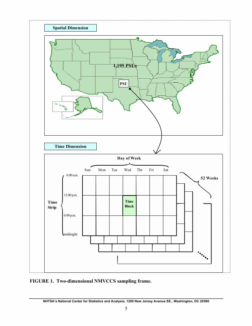
Taking into account these facts, NMVCCS used a two-dimensional sampling frame with

geographic location and time as surrogates of randomness of crash occurrence, where geographic

location was fixed while time was dynamically allocated on a weekly basis. Figure 1 depicts the

NMVCCS sampling frame. To lay out the sampling frame, the entire country was geographically

divided into 1,195 PSUs. Each PSU consisted of a central city, a county surrounding a central

city, an entire county, or a group of contiguous counties. Time dimension of the sampling frame

consisted of a combination of time of day and day of the week, to be referred to as time block.

Only the time period of 6 a.m. to midnight was considered in forming time blocks. This defines a

sampling unit within a PSU.


4

Spatial Dimension

PSU

Time Dimension

1,195 PSUs

6:00 a.m.

12:00 p.m.

6:00 p.m.

midnight

Time

Strip

Sun Mon Tue Wed Thr Fri Sat

Day of Week

Time

Block

52 Weeks


5

FIGURE 1. Two-dimensional NMVCCS sampling frame.

6. Sample Size


6

The response rate of sampling and investigating a crash successfully during a time block depends

on the effectiveness of notification, the researchers’ ability to get to the crash scene in time, and

the possibility of at least one crash occurrence in the time block. This resulted in a considerable

variation in response rates of different PSUs. To make the survey cost-effective, much care was

needed to achieve the maximum response rate.

Due to unavailability of sampling frame in advance as well as uncertainty of the response rate,

the sample size in this survey was determined from practical considerations rather than based on

the magnitude of sampling errors. The existing NASS-CDS infrastructure consisting of 24 PSUs

was used (for details of PSU selection in CDS, refer to section 8.1). As in the CDS, two

researchers were assigned per PSU and each researcher was required to investigate at most two

crashes per week. With these operational arrangements and adjustments, NMVCCS initially

targeted a sample of about 5,000 crashes per year (4,992 = 24 PSUs x 2 researchers per PSU x 52

weeks per year x 2 crashes per week/researcher).

7. Data Collection Methodology

Timely arrival of the researcher at the crash scene was crucial to NMVCCS data collection

because it gave the researchers an opportunity to gather first-hand information. For example,

they could discuss the circumstances of the crash with the crash-involved occupants while it was

still fresh in their minds and could reconcile the physical evidence with the witnesses’

descriptions.

For this purpose, the researchers monitored the EMS radio frequencies (or the police

notifications in certain PSUs) and when a crash notice was put out, the researchers traveled to the

crash scene. After arriving, they determined if the crash belonged to the target population. For a

qualified crash, an investigation was initiated by collecting information from all sources: the

crash scene, police, drivers, passengers, witnesses, and vehicles. The targeted information was

collected using a set of field forms and a portable computer.

8. Sampling Procedure

The selection of crashes in NMVCCS was accomplished through a multistage sampling

procedure. In each stage, samples were drawn with unequal probability based on the number of

crashes that occurred in a sampling unit, as estimated from the historical data. This gave a larger

sampling unit a higher chance of being selected in the sample. Specifically, NMVCCS sampling

procedure consists of the following five stages:

First Stage: Selection of PSU (geographical area as defined in NASS);

Second Stage: Selection of a sub-sampling unit in certain PSUs as necessary;

Third Stage: Selection of a time strip (a six-hour time interval between 6 a.m. and

midnight);

Fourth Stage: Selection of days of week for the selected time strip;

Fifth Stage: Selection of a crash within the selected time block, the combination of the

selected day of the week and the time strip.

In the subsequent sections, we provide the details of the selection procedure at each stage along

with the analytical formulas of the corresponding selection probability.

8.1. First Stage: Selection of PSU

This stage was adopted from NASS-CDS in order to use the NASS infrastructure and exploit the

resources available therein. Accordingly, the Unites States was divided into 1,195 PSUs, each

PSU consisting of a central city, a county surrounding a central city, an entire county, or a group

of adjacent counties. These 1,195 PSUs were stratified into 12 strata by geographic region

(Northeast, South, Central, and West) and urbanization type (large central city, large suburban

area, all others). Then, a total of 24 PSUs were selected with 2 PSUs per stratum roughly

proportional to the number of crashes in each stratum. Let πi be the inclusion probability of

PSU (i) in NMVCCS, which is the same as defined in the CDS sampling design. Detailed

information about CDS is provided in “NASS Crashworthiness Data System Analytical User’s

Manual.”2

8.2. Second Stage: Selection of a Sub-Sampling Unit in Certain PSUs Selection of PSU

Due to operational challenges, such as a huge volume of transmissions in many frequencies, a

large geographical area, traffic congestion, etc., certain PSUs required sub-sampling to maximize

the number of investigated crashes. In fact, due to one or more such reasons, only 5 PSUs

implemented sub-sampling. Depending upon the nature of the issue, different sub-sampling

procedures were adopted in different PSUs. For example, in one of these PSUs with a huge

volume of radio transmissions, three sub-sampling units were defined based on the police radio

frequencies, police jurisdictions, and geographical areas. This reduced not only the burden on the

researcher but also enhanced the chance of obtaining a qualifying crash within the selected PSU.

In forming the sub-sampling units, the crash total in each sub-sampling unit was also considered

to sustain sub-sampling. In two of the PSUs that had a large geographical area with historically

small number of crashes, each PSU was divided into two sub-sampling units according to the

EMS agencies operating in it. This helped researchers to place themselves within the sub-

sampling unit and to get to the crash site before the scene was cleared. In special cases, the

coverage of two sub-sampling units was overlapped in one PSU. This mode of operation helped

each sub-sampling unit to have enough crashes to sustain sub-sampling.

Whatever the reason or mode, sub-sampling was implemented on a weekly basis and was

independent of the selection of a time strip or a day of the week. Sub-sampling unit was selected

with probability proportional to the number of crashes estimated from NASS-CDS in the

previous year as the distribution of crashes over days of the week and time strips of the day had

been stable over the previous years, thereby producing a comparable estimate. In the subsequent

discussion, the number of crashes estimated from NASS-CDS will refer to the number of crashes

occurred in the previous year as coded in NASS-CDS and will be denoted by M with an

appropriate subscript.


7

Selection Probability of a Sub-Sampling Unit


8

Let Mij be the number of crashes occurred in sub-sampling unit ( j ) of PSU ( i ), and Mi be the

number of crashes occurred in PSU ( i ) as estimated from NASS-CDS. Then the inclusion

probability of a sub-sampling unit in week h is given by

Mπ ij

j|ih = . (2) Mi

However, in PSUs where some of police jurisdictions (or EMS agencies) belonged to two sub-

sampling units, the inclusion probabilities of the sub-sampling units are computed by the

formula,

Mπ ij

j|ih = , (3) M *

i

where *M

i is sum of the number of crashes in PSU ( i ) and the number of crashes in police

jurisdictions (or EMS agencies), which were included in both sub-sampling units in PSU ( i ). In

most of the PSUs, sub-sampling was not implemented and the entire PSU was treated as a single

sub-sampling unit. The inclusion probability of sub-sampling unit in these PSUs is one, i.e.,

π j|ih =1. (4)

8.3. Third Stage: Selection of a Time Strip

This stage consists of selecting a time interval during which the researchers in the selected PSU

monitored EMS and/or police radio frequencies to be able to get to a crash scene before it was

cleared. These time intervals are referred to as time strips. In most of the PSUs, the time period

of 18 hours was divided into 3 time strips: 6 a.m.–noon, noon-6 p.m., and 6 p.m.-midnight. A

time strip was selected on a weekly basis with probability proportional to the number of crashes

that occurred during the time strip, as estimated from NASS-CDS.

Selection Probability of a Time Strip

Let Mik

be the number of crashes occurred during the time strip ( k ) in PSU ( i ), and let Mi be

the number of crashes from 6 a.m. to midnight in PSU ( i ). Then the inclusion probability of the

time strip ( k ) of PSU ( i ) and week (h ), is computed by

Mπk ih

= ik

| . (5) M

i

In order to balance researcher’s workload and coverage of the time period from 6 a.m. to

midnight, the length of time strip was decided in accordance with the situation in each PSU. In

most of the PSUs, the length of time strip was 6 hours and only one time strip was chosen in

each week. However, in some PSUs with historically low frequency of crash occurrence, but

good cooperation with police or EMS agencies, a longer time strip was used. On the other hand,

in some PSUs a shorter time strip of 4.5 hours was used to avoid a potential bias of collecting

only crashes toward the beginning of the time strip due to high frequency of crash occurrence.

For PSUs with a longer time strip of 18 hours, this stage of time strip selection was skipped.

8.4. Fourth Stage: Selection of Days of Week

At the fourth stage, days of the week were selected after the selected time strip was overlaid over

seven days of the week. As a result, time blocks defined by the combination of a time strip and

days of the week were selected. Systematic probability proportional sampling3 was used with the

number of crashes that occurred during the time block as a measure of size, and that was

estimated from NASS-CDS data. This sampling method maximized the likelihood of having a

crash in the selected time block. Also, it spread the sampled time blocks more evenly over the

week so that the researcher had enough time to investigate each NMVCCS crash while it was

still fresh.

Selection Probability of Days of the Week

Let Mikl

denote the number of crashes occurred on day of the week (l) during the time strip ( k )

in PSU ( i ). Also, let Mik

be the number of crashes that occurred during the time strip ( k ) in

PSU ( i ). Then the inclusion probability of day of the week (l) in PSU ( i ), week (h ), and time

strip ( k ) is given by

Mπ = n ikl

l|ihk ih, (6)

Mik

where nih

is the number of days to be selected on week ( h ) in PSU ( i ). In most of the PSUs

four days were selected per week, i.e. nih

= 4, while in others, where available resources

permitted, nih

= 6. Hence, in most of the PSUs four time blocks of 6 hours were sampled per

week and all four time blocks were in the same time strip but belonged to different days of the

week.

In some rare cases, when one sampling unit (day of the week) was relatively much larger as

compared to other sampling units and when the number of the selected days was relatively large,

πl|ihk could be greater than one since systematic sampling method

4 was used. In such cases,

πl|ihk is set to 1, i.e., the day was selected with certainty. Suppose n

C days were selected with

certainty. Then, (n nih

−C) days were systematically selected with probability proportional to the

number of crashes from the remaining (7 − nC) days. The inclusion probability of day of the

week (l) is computed by Mπ l | ihk = (nih − n ) ikl

C , (7) M*

ik

where M *

ik is the number of crashes that occurred in time strip ( k ) of PSU ( i ), except for the

days of the week selected with certainty. If there isπl|ihk greater than one again, then the above

procedure is repeated until all nih

days of the week have been selected.


9

8.5. Fifth Stage: Selection of a Crash in the Selected Time Block

Once a time block was selected in a PSU, a researcher responded to all the notified crashes that

occurred during the time block using the notification means until a crash eligible for NMVCCS

was found or the time block was over, whichever happened first. The first eligible crash during

the time block was fully investigated by the researcher. In the subsequent discussion, the number

of crashes counted from NASS-CDS will refer to the number of crashes which occurred in the

current year and to which EMS had been dispatched as coded in NASS-CDS. This number will

be denoted by N with an appropriate subscript.

Selection Probability of a Crash in the Selected Time Block

The inclusion probability of a crash (m) in the selected time block is the ratio of the number of

crashes to be sampled to the number of crashes that actually occurred during the time block in

the current year and is given by

⎧ n⎪

ihjkl, if N

⎪ ihjkl ≠ 0N

π ihjkl

m|ihjkl = ⎨ (8) ⎪⎪ 0 , if ihjkl =⎩ N 0.

The number of crashes to be sampled in a time block, nihjkl , is one because only one crash is

supposed to be investigated in each time block. The total number of crashes that occurred in a

time block, denoted byNihjkl , is counted from the CDS database. If the CDS database shows that

there were no NMVCCS qualifying crashes in a time block, i.e.,Nihjkl = 0 , then the inclusion

probability of a crash in that time block is zero.

In a PSU, where sub-sampling was implemented, the inclusion probability of a crash (m) in a

certain time block is given by

⎧ Ji

⎪ N

⎪ nihjkl

⎪ihjkl

∑⋅ j=1

, if N ≠ 0π m|ihjkl = ⎨ ihjkl

Nihjkl Nihkl (9) ⎪⎪⎩⎪ 0 , if Nihjkl = 0.

where Ji is the number of sub-sampling units in PSU (i), and N

ihkl is the total number of crashes

in a time block in PSU (i) counted from CDS database. In general, sum of crashes that occurred

in a time block in each sub-sampling unit in a PSU is equal to the number of crashes in the same

∑J

NihjklJij=

time block and PSU, i.e. ∑Nihjkl = Nihkl . Then, the adjustment factor, 1

, becomes one j=1 Nihkl


10

and the formulas in (8) and (9) become the same. But there were certain PSUs where some of

police jurisdictions (or EMS agencies) were included in two sub-sampling units as mentioned in

section 8.2. In this case, ∑Ji

Nihjkl ≠ Nihkl because the number of crashes in the police j=1

jurisdictions (or EMS agencies) included in both sub-sampling units has been counted twice

in∑Ji

Nihjkl . The inclusion probability of crash (m) in this case is adjusted by multiplying the j=1

J

∑i

Nihjklj=

inclusion probability by the adjustment factor 1

as shown in the formula (9). Nihkl

While the number of crashes to be sampled in a time block, nihjkl , is one, the number of crashes

∗actually sampled, denoted by nihjkl , is one or zero. In case a sampled time block elapsed without

a qualifying crash, the time block was considered empty and no substitution was allowed for ∗such a case, i.e. nihjkl =0. On the other hand, if a crash was actually sampled in a time block, then

the total number of crashes in that time block, Nihjkl , must be greater than or equal to one. In

= ∗some time blocks, however, N 0ihjkl , although nihjkl =1 because the crashes in CDS data are not

completely consistent with the crashes in NMVCCS. The number of crashes in such time blocks

is estimated under the assumption that there must be at least one crash.

8.6. Time Block Reduction

Due to researcher’s vacation, sick leave, military service, resignation, or other reasons, some of

the sampled time blocks were not used. In NMVCCS, this is termed as “time block reduction.”

Time blocks to be removed due to such reasons were pre-marked from the sampled time blocks

by random sampling on a weekly basis. In order to account for such exigencies, the probability

of a sampled time block to be used was considered in the selection process.

Probability of a Sampled Time Block to Be Used

The probability of a sampled time block to be used, γih

, is computed for each week in the

selected PSU. Let nih

be the number of sampled time blocks of week ( h ) in PSU ( i ), and n*ih

be

the actual number of used time blocks. Let ni.

be the total number of weeks in PSU ( i ) during

one year (the sampling period considered in NMVCCS), and *ni.

be the number of weeks with at

least one used time block. Then γih

is the product of the probability of the sampled time block to

be used in week (h ) and the probability of week (h ) to be used in the sampling period, i.e.

n*n*

γ = ih i

ih⋅ . . (10)

n nih i.


11

9. Estimation Procedure


12

In order to make the NMVCCS sample a nationally representative sample, a comprehensive

estimation procedure is necessary that takes into account the crash selection process. The

weighting procedure used in NMVCCS consists of mainly two steps, design weight and its

adjustment. After the design weight is obtained that reflect the selection probability in each stage

of the sampling design, adjustments are made to the design weights for missing crashes resulting

from the operational difficulties or limitations.

9.1. Design Weight

Design weight is calculated by taking the reciprocal of the inclusion probability of a crash, which

is the multiplication of the inclusion probabilities at all stages of the sampling procedure

described in the previous section. Specifically,

π ihjklm = π i π j|ih π k|ih π l|ihk π m|ihjkl γ ih , (11)

where

πi is the inclusion probability of PSU (i) described in section 8.1,

π j|ih is the inclusion probability of a sub-sampling unit (j) in the selected PSU (i) for week (h)

given by (2),

πk |ih is the inclusion probability of a time strip (k) in the selected PSU (i) for week (h) given by

(5),

πl|ihk is the inclusion probability of a day (l) of week in the selected time strip (k) and PSU (i) for

week (h) given by (6),

π m|hijkl is the inclusion probability of a crash (m) in the selected time block, i.e, time strip (k) and

day of week (l), sub sampling-unit (j) and PSU (i) for week (h) given by (8),

γih

is the probability of a sampled time block to be used in PSU (i) and week (h) given by (10).

Thus, the design weight of a NMVCCS crash, wihjklm , computed for all used time blocks is given

by

⎧ π −1

⎪ ihjklm , if π ihjkl ≠ 0wihjklm = ⎨ (12)

⎪⎩ 0 , if π ihjkl = 0,

where π ihjklm is given by (11).

9.2. Adjustment of Design Weight for Time Blocks With a Missing Crash

As mentioned earlier, the design weights are computed for all used time blocks. However, some

of the used time blocks were empty because there was no crash sampled and investigated during

the time blocks. There are two situations in which this could happen.

Situation 1: When according to CDS data, there was actually no NMVCCS qualifying crash

during a time block, the time block is empty and the corresponding design weight becomes zero

from (8), (11), and (12).

Situation 2: Sometimes, however, a crash was not sampled even though CDS data showed that

there were NMVCCS qualifying crashes during the time block. This crash is called a “missing

crash” and the empty time block is termed as a time block with missing crashes. Missing crashes

were caused mainly due to two reasons: (a) the crash scene had already been cleared when the

researcher arrived, i.e., the two on-scene requirements listed in section 4 are not satisfied, and (b)

the researcher missed the notification from the EMS or police frequencies due to operational

restrictions.

While there is no adjustment made in situation 1, the design weights must be adjusted to

compensate the missing crashes in situation 2. In NMVCCS, weighting-class adjustment

method5 is implemented for such crashes with week and PSU as classes. As a result, the design

weights of time blocks with missing crashes are distributed to other time blocks that have a

sampled crash through two-level adjustments: week and PSU, as described in the following

sections.

9.2.1. Adjustment at Week level

At the week level, the design weights of time blocks with missing crashes are distributed to the

other time blocks which contain a sampled crash in the same week and PSU.

∗Let nihjkl and nihjkl , respectively, be the number of crashes to be sampled and the number of

crashes actually sampled in a time block. Since only one crash is to be selected in each time ∗ ∗block, nihjkl = 1 . While n = 1ihjkl if a crash is sampled, n = 0ihjkl if a crash is not sampled. Let

Uih

be a set of subscripts ( j,k, l) of used time blocks during the week (h) in PSU (i), where

subscripts ( j,k, l) represent the selected sub-sampling unit (j), time strip (k), and day of the

week (l). The sum of the design weights for all used time blocks during the week (h) in PSU (i)

is given by nih jkl

Sih = ∑ ∑wihjklm . (13) ( 1j ,k ,l )∈ =Uih m

Also, the sum of the design weights for all time blocks with a sampled crash during the week (h)

in PSU (i), is given by nih

∗Sih = ∑ ∑jkl

wihjklm ⋅ I ∗ ,n (14)

ih jkl( j ,k ,l )∈Uih m=1

⎧⎪ ∗1 , if nih jkl = 1

where wihjklm is given by (12) and I ∗ nih jkl

= ⎨ ∗0 , nih jkl =⎩⎪ if 0.

Then the adjustment factor for the time blocks with missing crashes at this level is given by


13

⎧ ∗ ∗S if S > ∗S 0 1ih ih ih and nihjkl =⎪ ∗ ∗

Aihjkl = ⎨ 0 if S 0ih > and n = 0ihjkl . (15) ⎪ ∗⎩ 1 if S = 0ih

∗The week-level adjusted weight,wihklm

, is obtained by multiplying this adjustment factor by

design weights, i.e. ∗wihklm = Aihjkl wihjklm . (16)

∗The first factor, Sih

/Sih

in (15) distributes the design weights of the time blocks with missing

crashes are distributed to the other time blocks with a sampled crash in the same week and PSU.

The second factor sets the weights of the time blocks with missing crashes to zero. In the case

that all used time blocks in a certain week of PSU have missing crashes, an adjustment for the

missing crash is carried over to the next adjustment level of PSU by the third factor as discussed

in the following section.

9.2.2. Adjustment at PSU Level

Adjustment of design weights at PSU level is required if all used time blocks in a certain week in ∗a PSU are empty, i.e. S = 0ih

. The design weights of such time blocks are distributed to other

weeks with at least one sampled crash in the same PSU.

Let Hi be the set of subscripts of weeks with at least one used time block in PSU (i), and *

Hi be

the set of subscript of weeks with at least one sampled crash in PSU (i). Then the sum of the

week-level adjusted weights of all used time blocks in PSU (i) is

S = w*i ∑ ihjklm , (17) h∈H

∑i ( j ,k ,l )∈Uih

and the sum of week-level adjusted weights for all weeks that have at least one sampled crash in

PSU (i) is

∗S *

i = ∑ ∑wihjklm . (18) ∈ *h H ( j ,k ,l ) U

i∈ ih

The adjustment factor of time blocks with missing crashes at this level is given by

⎧ ∗ ∗S S , if S > 0

A i i ih

ih = ⎨ . (19) ⎩

∗0, if Sih = 0

The first factor in (19) distributes the design weights of time blocks with missing crashes in a

whole week over the time blocks of the other weeks that have at least one sampled crash in the

same PSU. The weights of these time blocks with missing crashes become zero by the second

factor. Thus, the adjusted final weights of NMVCCS crashes are obtained by

∗∗ = ∗wihjklm Aihwihjklm . (20)


14

10. Some Highlights of NMVCCS


15

In this section, using the data obtained from July 2005 to June 2006, some statistics are presented

to demonstrate the performance of NMVCCS according to the sampling design. These include

the number of sampled time blocks, and the number of qualified and initiated crashes, etc.

Additionally, as examples, national estimates related to the number of vehicles involved in a

crash and the percentages of crashes with critical reasons for critical pre-crash event attributed to

driver are obtained by applying the NMVCCS estimation procedure. For further information

about NMVCCS such as data coding, data quality process, etc., refer to the report titled,

“NMVCCS 2005 Coding and Editing Manual.” 6

10.1. Sampling Statistics

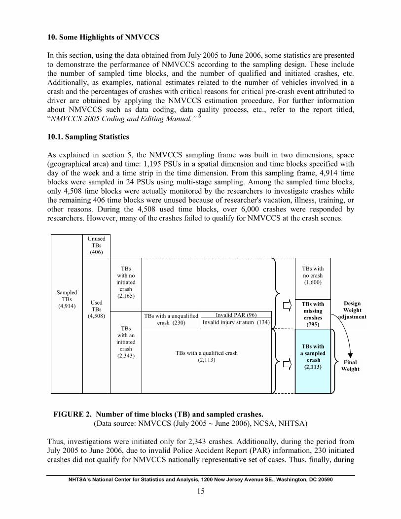
As explained in section 5, the NMVCCS sampling frame was built in two dimensions, space

(geographical area) and time: 1,195 PSUs in a spatial dimension and time blocks specified with

day of the week and a time strip in the time dimension. From this sampling frame, 4,914 time

blocks were sampled in 24 PSUs using multi-stage sampling. Among the sampled time blocks,

only 4,508 time blocks were actually monitored by the researchers to investigate crashes while

the remaining 406 time blocks were unused because of researcher's vacation, illness, training, or

other reasons. During the 4,508 used time blocks, over 6,000 crashes were responded by

researchers. However, many of the crashes failed to qualify for NMVCCS at the crash scenes.

Sampled

TBs

(4,914)

Used

TBs (4,508)

Unused

TBs (406)

TBs

with an

initiated

crash

(2,343)

TBs

with no

initiated

crash

(2,165)

TBs with a qualified crash

(2,113)

TBs with a unqualified

crash (230)

TBs with

a sampled

crash

(2,113)

TBs with

no crash

(1,600)

TBs with

missing

crashes

(795) Invalid injury stratum (134)

Final

Weight

Design

Weight

adjustment Invalid PAR (96)

FIGURE 2. Number of time blocks (TB) and sampled crashes.

(Data source: NMVCCS (July 2005 ~ June 2006), NCSA, NHTSA)

Thus, investigations were initiated only for 2,343 crashes. Additionally, during the period from

July 2005 to June 2006, due to invalid Police Accident Report (PAR) information, 230 initiated

crashes did not qualify for NMVCCS nationally representative set of cases. Thus, finally, during

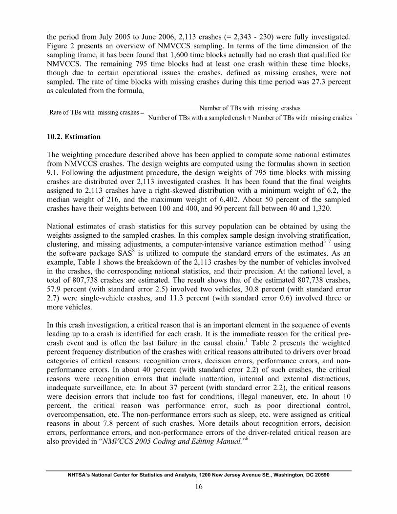
the period from July 2005 to June 2006, 2,113 crashes (= 2,343 - 230) were fully investigated.

Figure 2 presents an overview of NMVCCS sampling. In terms of the time dimension of the

sampling frame, it has been found that 1,600 time blocks actually had no crash that qualified for

NMVCCS. The remaining 795 time blocks had at least one crash within these time blocks,

though due to certain operational issues the crashes, defined as missing crashes, were not

sampled. The rate of time blocks with missing crashes during this time period was 27.3 percent

as calculated from the formula,

= Number of TBs with missing crashes Rate of TBs with missing crashes .

Number of TBs with a sampled crash + Number of TBs with missing crashes

10.2. Estimation

The weighting procedure described above has been applied to compute some national estimates

from NMVCCS crashes. The design weights are computed using the formulas shown in section

9.1. Following the adjustment procedure, the design weights of 795 time blocks with missing

crashes are distributed over 2,113 investigated crashes. It has been found that the final weights

assigned to 2,113 crashes have a right-skewed distribution with a minimum weight of 6.2, the

median weight of 216, and the maximum weight of 6,402. About 50 percent of the sampled

crashes have their weights between 100 and 400, and 90 percent fall between 40 and 1,320.

National estimates of crash statistics for this survey population can be obtained by using the

weights assigned to the sampled crashes. In this complex sample design involving stratification,

clustering, and missing adjustments, a computer-intensive variance estimation method5 7

using

the software package SAS8 is utilized to compute the standard errors of the estimates. As an

example, Table 1 shows the breakdown of the 2,113 crashes by the number of vehicles involved

in the crashes, the corresponding national statistics, and their precision. At the national level, a

total of 807,738 crashes are estimated. The result shows that of the estimated 807,738 crashes,

57.9 percent (with standard error 2.5) involved two vehicles, 30.8 percent (with standard error

2.7) were single-vehicle crashes, and 11.3 percent (with standard error 0.6) involved three or

more vehicles.

In this crash investigation, a critical reason that is an important element in the sequence of events

leading up to a crash is identified for each crash. It is the immediate reason for the critical pre-

crash event and is often the last failure in the causal chain.1 Table 2 presents the weighted

percent frequency distribution of the crashes with critical reasons attributed to drivers over broad

categories of critical reasons: recognition errors, decision errors, performance errors, and non-

performance errors. In about 40 percent (with standard error 2.2) of such crashes, the critical

reasons were recognition errors that include inattention, internal and external distractions,

inadequate surveillance, etc. In about 37 percent (with standard error 2.2), the critical reasons

were decision errors that include too fast for conditions, illegal maneuver, etc. In about 10

percent, the critical reason was performance error, such as poor directional control,

overcompensation, etc. The non-performance errors such as sleep, etc. were assigned as critical

reasons in about 7.8 percent of such crashes. More details about recognition errors, decision

errors, performance errors, and non-performance errors of the driver-related critical reason are

also provided in “NMVCCS 2005 Coding and Editing Manual.”6


16

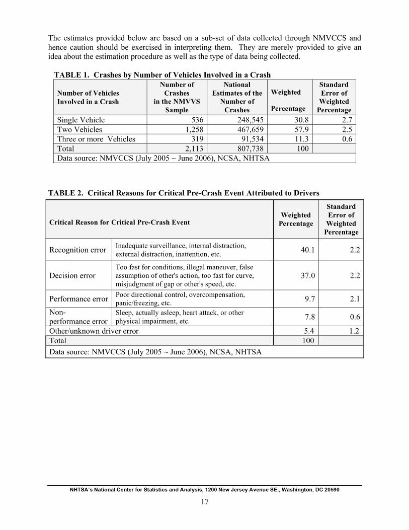
The estimates provided below are based on a sub-set of data collected through NMVCCS and

hence caution should be exercised in interpreting them. They are merely provided to give an

idea about the estimation procedure as well as the type of data being collected.


17

TABLE 1. Crashes by Number of Vehicles Involved in a Crash

Number of National Standard

Number of Vehicles Crashes Estimates of the Weighted Error of

Involved in a Crash in the NMVVS

Sample

Number of

Crashes Percentage Weighted

Percentage

Single Vehicle 536 248,545 30.8 2.7

Two Vehicles 1,258 467,659 57.9 2.5

Three or more Vehicles 319 91,534 11.3 0.6

Total 2,113 807,738 100

Data source: NMVCCS (July 2005 ~ June 2006), NCSA, NHTSA

TABLE 2. Critical Reasons for Critical Pre-Crash Event Attributed to Drivers

Standard

Critical Reason for Critical Pre-Crash Event Weighted

Percentage

Error of

Weighted

Percentage

Recognition error Inadequate surveillance, internal distraction,

external distraction, inattention, etc. 40.1 2.2

Decision error Too fast for conditions, illegal maneuver, false

assumption of other's action, too fast for curve,

misjudgment of gap or other's speed, etc. 37.0 2.2

Performance error Poor directional control, overcompensation,

panic/freezing, etc. 9.7 2.1

Non-

performance error Sleep, actually asleep, heart attack, or other

physical impairment, etc. 7.8 0.6

Other/unknown driver error 5.4 1.2

Total 100

Data source: NMVCCS (July 2005 ~ June 2006), NCSA, NHTSA

11. References


18

1. Perchonok, K. Accident Cause Analysis, Cornell Aeronautical Laboratory, Inc.,

July 1972.

2. NASS Crashworthiness Data System Analytical User’s Manual. National Center for

Statistics and Analysis, 2006. Washington, DC: National Highway Traffic Safety

Administration.

3. Cochran, W. Sampling Techniques. John Willey and Sons, Inc., New York, 1977.

4. Madow, W.G. On the Theory of Systematic Sampling, II, Annals of Mathematical

Statistics, 20, 333 -354, 1949.

5. Lohr, S. L., Sampling: Design and Analysis. Duxbury Press, 1999.

6. NMVCCS 2005 Coding and Editing Manual, National Center for Statistics and

Analysis, 2007. Washington, DC: National Highway Traffic Safety Administration.

7. Siller, A.B., & Tompkins, L. The Big Four: Analyzing Complex Sample Survey Data

Using SAS, SPSS, STATA, and SUDAAN, Proceedings of the Thirty-first Annual

SAS Users Group International Conference, Cary, NC. SAS Institute Inc. 2006.

8. SAS/STAT 9.1 User’s Guide, SAS Institute Inc., Cary, NC. 2004, pp. 4,185-4,240.

DOT HS 810 930April 2008

sampling design used in the national motor vehicle crash

Documents