sandros: a dynamic graph search algorithm for …amato/courses/689/papers/sandros_ra_t… · 390...

390 IEEE TRANSACTIONS ON ROBOTICS AND AUTOMATION, VOL. 14, NO. 3, JUNE 1998

SANDROS: A Dynamic Graph SearchAlgorithm for Motion Planning

Pang C. Chen and Yong K. Hwang,Member, IEEE

Abstract—We present a general search strategy called SAN-DROS for motion planning, and its applications to motion plan-ning for three types of robots:

1) manipulator;2) rigid object;3) multiple rigid objects.

SANDROS is a dynamic-graph search algorithm, and can be de-scribed as a hierarchical, nonuniform-multiresolution, and best-first search to find a heuristically short motion in the configu-ration space. The SANDROS planner is resolution complete, andits computation time is commensurate with the problem difficultymeasured empirically by the solution-path complexity. For manyrealistic problems involving a manipulator or a rigid object withsix degrees of freedom, its computation times are under 1 minfor easy problems involving wide free space, and several minutesfor relatively hard problems.

Index Terms—Collision avoidance, configuration space, motionplanning, path planning.

I. INTRODUCTION

T HE motion planning problem is the problem of findinga collision-free motion for one or more moving objects

between the start and the goal configurations. A moving objectcan be a rigid object, or a jointed object such as an industrialmanipulator. Motion planning has received much attention forthe past two decades from robotics in order to

1) automatically generate the movements of mobile robotsand their arms;

2) automatically plan and program the motions of man-ufacturing robots and mechanical parts in assemblingproducts.

Automation of motion planning offers a number of ad-vantages over the existing alternatives. It relieves humanworkers of the continual burden of detailed motion designand collision avoidance, and allows them to concentrate onthe robotic tasks at a supervisory level. Robots with anautomatic motion planner can accomplish tasks with fewer,higher-level operative commands. Robotic tele-operations canthen be made much more efficient, as commands can begiven to robots at a coarser time interval. With an automaticmotion planner and appropriate sensing systems, robots can

Manuscript received January 16, 1996; revised January 8, 1997. Thiswork was supported by the U.S. Department of Energy under Contract DE-AC04-94AL85000. This paper was recommended for publication by AssociateEditor M. Peshkin and Editor S. Salcudean upon evaluation of the reviewers’comments.

The authors are with the Intelligent Systems and Robotics Center, SandiaNational Laboratories, Albuquerque, NM 87185 USA.

Publisher Item Identifier S 1042-296X(98)02665-2.

adapt quickly to unexpected changes in the environmentand be tolerant to modeling errors of the work space. Inmanufacturing applications, an automatic motion planner canbe used to verify the assemblability of a product by findingthe motion of each part during the assembly, and to plan themotions of robot manipulators performing operations such ascutting, welding, and assembling. This reduces the productdesign time by enabling product designers to make necessarymodifications at the design stage, and it also reduces the setuptime of manufacturing lines by enabling rapid programmingof manipulator motions.

Although humans have a superb capability to plan motionsof their body and limbs effortlessly, the motion planningproblem turns out to be a high complexity problem [47]. Thebest known algorithm [9] has a complexity that is exponentialin the number of degrees of freedom (DoF), and polynomialin the geometric complexities of the robot and obstacles inits environment. For motion planning problems in the three-dimensional (3-D) space where 6, existing completealgorithms [6], [40] that guarantee a solution often takes tens ofminutes of computation time. On the other hand, fast heuristicalgorithms [27] may fail to find a solution even if there is one.

Because of the proven complexity of motion planning, thedevelopment of a motion planner capable of solving all prob-lems in a short time is unlikely. Hence, the next best alternativeis to have an algorithm with performance commensurate withtask difficulty. (Because there is no set of benchmark problems,we measure the task difficulty empirically by the complexityof the solution path, e.g., the number of monotone segmentscomprising the path and the clearance to obstacles alongthe path.) In this paper, we present an efficient, resolution-complete search framework called SANDROS that results inmotion planners with exactly this characteristic. It can be usedfor motion planning of a serial-linkage manipulator, a rigidobject or multiple rigid objects, and can solve “easy” problemsquickly and “difficult” problems systematically with a gradualincrease of computation time. For typical problems involving6-DoF robots, the running time ranges from under 1 min to10 min.

This paper summarizes our work reported in [12], [26], and[29]. Previous work is reviewed in Section II. In Section III,the SANDROS search strategy is described and used todevelop motion planners for a manipulator, a rigid object andmultiple rigid objects. Their performance is illustrated withexamples in Section IV, and conclusions and future work arediscussed in Section V. Before we go on, we define someterms here. Therobot refers to the moving object, and the

U.S. Government work not protected by U.S. copyright

CHEN AND HWANG: DYNAMIC GRAPH SEARCH ALGORITHM FOR MOTION PLANNING 391

configuration vector of a robot is a vector of real-valuedparameters that completely determines the position of everypoint of the robot. For a manipulator, the set of joint anglescan be used to define its configuration, whereas for a rigidobject the position of a reference point of the object and itsorientation about that point serve as its configuration vector.The length of the configuration vector is defined as the DoFof the robot. The configuration space (C-space) is the spaceof all possible configurations of the robot. We use the terms“free,” “collision-free,” and “feasible” interchangeably. Sinceour motion planners use only the distance information betweenthe robot and obstacles, they are independent of the object rep-resentation scheme, as long as the distance can be computed.

II. PREVIOUS WORK

Comprehensive reviews of the work on motion planningcan be found in [35], [28]. In this section, we concentrateon major work on manipulators and rigid objects. Planningmotions for a general 6-DoF robot is very difficult, and themost efficient motion planners that are guaranteed to finda solution if one exists run in tens of minutes for difficultproblems. It should be noted that the computation timesfor 6-DoF robots are important, because they are useful forgeneral purpose manipulation and in wide use for industrialapplications such as spot-welding and painting. (A 6-DoFrobot is required to arbitrarily position and orient an objectwithin the work space.) There are several complexity re-sults for various motion planning problems. In [47], planningthe motion of a polyhedral manipulator among polyhedralobstacles is proven to be PSPACE-hard. The problem oftranslating multiple rectangles are shown to be PSPACE-hardin [24], and PSPACE-complete in [25]. An upper bound forpath planning is established in [49], which gave an exactalgorithm that is polynomial in the geometric description of therobot and environment, and doubly exponential in DoF. Thedoubly exponential component is later improved to a singleexponential with theroadmapalgorithm in [9]. To sum up,motion planning algorithms are likely to be exponential inDoF.

Motion planners can be classified into two categories:

1) complete;2) heuristic.

Complete motion planners can potentially require long com-putation times but can either find a solution if there is one,or prove that there is none. Heuristic motion planners arefast (typically take seconds), but they often fail to find asolution even if there is one. Presently, all implementationsof complete algorithms are resolution-complete, meaning theyguarantee a solution at the resolution of the discretization usedin the algorithm. For this reason, we use the termcompletealgorithm to meanresolution-completealgorithm for the restof this paper. Motion planning approaches are reviewed first,followed by motion planners specifically for a manipulator,a rigid object and multiple rigid objects, respectively. For afair comparison of planners’ efficiency, computation times arecalibrated to estimated running times on a modern 200 MHzworkstation.

A. Motion Planning Approaches

To date, motion planning approaches can be classified intofour categories [35]:

1) skeleton;2) cell decomposition;3) potential field;4) subgoal graph.

In the skeleton approach, the free space is represented by anetwork of one-dimensional (1-D) paths called askeleton,and the solution is found by first moving the robot onto apoint on the skeleton from the start configuration and fromthe goal, and connecting the two points via paths on theskeleton. This approach is intuitive for two-dimensional (2-D)problems, but becomes harder to implement for higher-DoFproblems. Algorithms based on the visibility graph [39], theVoronoi diagram [44], and thesilhouette(projection of ob-stacle boundaries) [9] are examples of the skeleton approach.In the cell-decomposition approach [45], [51] the free spaceis represented as a union of cells, and a sequence of cellscomprises a solution path. For efficiency, hierarchical trees,e.g, octree, are often used. In the potential-field approach, ascalar potential function that has high values near obstaclesand the global minimum at the goal is constructed, and therobot moves in the direction of the negative gradient of thepotential. In the subgoal-graph approach, subgoals representkeyconfigurations expected to be useful for finding collision-free paths. A graph of subgoals is generated and maintainedby a global planner, and a simple local planner is used todetermine the reachability among subgoals. This two-levelplanning approach has turned out to be the most effective pathplanning method, and is first reported in [18].

B. Manipulator Problems

The first complete planner for a 3-DoF manipulator is devel-oped using an octree representation of the C-space obstaclesin [17], while sequential construction of the C-space obstaclesis used in [40] to plan motions for a general serial manipulatorin the 3-D world space. The latter computes the free regionsof the C-space by successively computing feasible ranges foreach link, starting from the base of the robot. For example,for each point in the feasible ranges ofjoint , the feasibleranges ofjoint are computed. These ranges are groupedinto regions, and the search for a path is done on the graph ofthese regions. The number of feasible ranges are exponentialin DoF, and this algorithm is likely to take a few minutes inour estimation for a 4-DoF problem.

Kondo [34] has reported a fast grid search algorithm thatuses several heuristics to favor different motions during search.The effectiveness of a heuristic is measured by ,where is the length of the path from the start to the currentsearch configuration, and is the number of the collisionchecks performed by the heuristic to generate the path. Thenumbers of collision detections reported by this planner areroughly on the same order of magnitude as those of our plan-ner. Kondo’s algorithm is effective when the solution path liesin a narrow winding tunnel because of the grid search, but canspend a lot of computation exploring a large dead-end space.This algorithm is also used to plan motion of a rigid body.


Probabilistically complete algorithms find a solution withprobability 1 given long enough computation time, and isa typical characteristic of randomized algorithms. In [4] apotential-field based method called RPP uses gradient descentto approach the goal configuration. If it gets stuck at a localminimum, the planner uses random walks to escape fromthe local minimum. This process is repeated until the robotreaches the goal. A more elaborate algorithm, also potentialbased, applying a dynamic programming technique to varioussubmanifolds of the C-space is presented in [3]. It is slowerbut capable of solving harder problems than RPP. The randomnature of RPP prevents one from devising an unsolvableproblem, but when the solution path has to pass througha narrow space, it takes a long time to find this passagewith random movements. A subgoal graph calledprobabilisticroadmapis developed in [31] to overcome this problem. Ran-dom configurations are generated and those without collisionsare kept in the graph. A simple local planner is used to checkthe reachability between subgoals. The graph is augmentedwith additional subgoals in the cluttered C-space to increasethe connectivity of the graph. Finally, path planning is doneby connecting the start and goal to subgoals on the graph andtraversing the graph to connect the two subgoals. The maindifference between this and our algorithm is that our algorithmgenerates subgoals hierarchically and incrementally until theproblem is solved, while theirs generates all the subgoals atthe beginning. When solving multiple problems in the sameenvironment, the entire subgoal graph can be generated beforesolving the problems, or a learning technique can be used toprogressively build the graph while solving the problems oneby one [11]. Both of the probabilistic algorithms can also beused for rigid objects.

Padenet al. [45] have presented a complete algorithm whichcomputes the free C-space in the -tree of rectangularcells using the Jacobian of the robot. Although developedfor a manipulator, generalization to a rigid body is straightforward. The bound on the Jacobian gives the maximumdistance traveled by any point on the robot when the robotconfiguration is varied inside a unit sphere. Thus, the distancebetween the robot and objects divided by the bound on theJacobian gives a lower bound on the radius of the collision-free sphere in the C-space. For a manipulator with a long reachor an elongated object, however, the large norms of Jacobiansallow only a small volume of the free C-space to be computedat a time. It takes about 1 s to solve a 2-DoF problem.

There are many heuristic motion planners with computationtimes proportional to their capabilities. For example, thealgorithm in [46] uses a global planner based on the Voronoidiagram and a local planner based on the virtual spring method(a potential field variant), and its computation times are under1 min for an easy 6-DoF problem in 3-D. On the otherhand, the algorithm in [22], [23] is much more elaborate, anduses a sequential framework to decompose the original DoF-dimensional problem into a sequence of smaller-dimensionalproblems. Given the path of theth joint parameterized by,it plans the path of the ( 1)th joint in the space usinga visibility or potential-field method. This algorithm solvestwo problems involving a 7-DoF robot in relatively cluttered

environments in 10 min and 1 h. For many applications, aspecialized heuristic motion planner is often sufficient, anda computationally expensive complete planner may not beneeded. We note that our manipulator motion planner exploitsthe sequential structure of a manipulator as done in [22] and[40].

C. The Classical Mover’s Problem

There has been a lot of work on the classical mover’sproblem, i.e., motion planning for a rigid object. For the 2-Dproblem (3 DoF) an octree is used in [7] to develop acomplete planner, while for the 3-D problem (6 DoF) thefirst implemented planner is a grid search algorithm [14]. Itbuilds up a lattice of points in the C-space, and collision checkfor a point is done by evaluating the boundary equations ofthe C-space obstacles. It uses several heuristics to speed upthe search. Its computation time is estimated to be tens ofminutes for hard problems. In [2], an exact motion planner fora polygonal robot with 3 DoF is developed. This algorithmbuilds an exact geometric description of the C-space obstaclesusing edge-edge contact conditions.

A subgoal-graph approach is used in [20] to plan motions ofa polygon in 2-D. Random subgoals are generated during thesearch, while a local planner is used to connect the subgoals. Itsolves 2-D, 3-DoF problems under 1 min, and is one of the firstrandomized path planners. Another subgoal-graph approach,reported in [6], uses a genetic algorithm to select subgoals andsearch collision-free paths between subgoals. It is a completeplanner with run times in tens of minutes for difficult 6-DoFproblems. For other complete rigid-body motion planners, seealso the previous section.

In [27], a fast heuristic planner for 3-D is developed basedon the potential field. It finds a path for the reference point ofthe robot first, and moves robot’s reference point along thispath while aligning robot’s longest axis tangentially to thepath to minimize the swept volume. If a collision occurs, itgenerates feasible robot orientations in that region, and usesthese as intermediate subgoals. This algorithm is fast andeffective for convex robots, but fails on problems with highlyconcave robots like that in Fig. 9.

For a 2-D rigid object the C-space is only 3-D, and abrute force search algorithm runs in a few minutes. A bruteforce search would discretize the C-space, check whether thereis a collision at each of these points, and find a connectedsequence of collision-free points in the C-space. In fact,such an algorithm has been implemented in [37]. For the3-D classical mover’s problems, however, a more efficientalgorithm is still needed to search 6-DoF space.

D. The Multimovers’ Problem

The multimovers’ problem is the problem of finding pathsfor several robots between their initial and goal configurations.Robots have to avoid one another as well as obstacles. Thealgorithms for this problem can be classified into centralizedand distributed planning. In centralized planning, motions ofall robots are planned by a single decision maker. Centralizedplanning can be further divided into algorithms with or without


priority among the robots. In certain applications, there are pri-ority relations among the relative importance of the missionsof robots. In other cases, the priority is artificially imposed todecompose the multiple movers’ problem into a sequence ofsingle-mover’s problems. This, however, introduces a loss ofoptimality as well as completeness, i.e., the planned motionof a robot may preclude the motion of another robot with alower priority.

A centralized approach is reported in [16], where theobstacles in the composite C-space are constructed to planpaths for two robots. In case there is a conflict betweenrobots, the burden of collision avoidance is imposed on therobot with a lower priority. Motion planning of many square-shaped robots in the plane is presented in [8]. This algorithmhas an application in an assembly cell, where multiple robotsmove on the ceiling, delivering parts and performing assemblyoperations. This algorithm tries to move as many robots aspossible in straight lines, and minimizes the number of robotsthat have to make turns. Recently, game theory is used in [36]to plan paths of robots while optimizing multiple objectives.Robots are constrained to move on a skeleton such as theVoronoi diagram, and the concept of Nash equilibrium is usedto schedule robot motions on the skeleton. A randomizedapproach is used to plan motions of multiple manipulators in[33]. This algorithm plans manipulator motions that move anobject from one position to another. The path of the objectis planned first, and the motion of each manipulator thatmoves the object along the planned path is computed bysolving inverse kinematics. Since manipulators cannot carrythe object outside their reachable space, the planner assignsspecific manipulators to carry the object at different portionsof the path. Although this algorithm is not complete, it isefficient and solves many realistic problems. Finally, RPP andthe probabilistic roadmap are used in the composite C-space toplan motions of multiple robots in [5] and [48], respectively.

A distributed planning approach is taken in [53] to planpaths for circular robots. Each robot plans its own path usingthe visibility graph. When conflicts arise among robots, it isreported to the central coordinator called theblackboard,which issues priorities based on the tasks and current state.Another decentralized approach for circular robots of differentsizes is presented in [38]. A quadtree is used for path planningalong with a Petri net formulation to resolve the conflictsamong robots.

III. A LGORITHM

We have developed an efficient, resolution-complete al-gorithm capable of planning motions for arbitrary robotsoperating in cluttered environments. We plan robot motionsin the C-space, and make the standard assumption that ifa task is solvable, a solution path can be represented by asequence of unit movements in the C-space, discretized to auser-specified resolution. To handle the high dimensionalityof the C-space and search complexity, we make the followingdesign decisions without sacrificing completeness.

1) First, we determine whether a given point in the C-space is in free space by computing the distance [19]

between the polyhedral robot and obstacles. (As longas a CAD modeler supports a distance routine, it canbe used with our motion planner.) Contact conditionscan be used [14], [40], but equations describing contactboundaries are nonlinear, and detecting intersections ofthese boundaries is computationally expensive. The useof distance makes our algorithm independent of objectmodels, and enables the selection of ‘safer’, i.e., largerclearance, configurations for the robot.

2) Second, we use a two-level hierarchical planning schemeto reduce memory requirements, as done in [18]. It isdifficult to store all the collision-free points even if wecould compute them all, since the C-space typicallyhas an enormous number of points even at a coarseresolution. We circumvent this problem by planningat two levels using a global and a local planner. Theglobal planner keeps track of reachable, unreachable,and potentially reachable portions of the C-space, andthe local planner checks the reachability of a portionof the space from a point. If a portion of space isreachable from a point, then the corresponding collision-free motion needs not be stored, since they can be readilyrecovered by the local planner at any later stage of thealgorithm. But if the distance computation is expensive,it is more efficient to store the motion.

3) Third, we use a multiresolution approach to reducesearch time. An exhaustive search for a collision-freemotion is prohibitive because of the enormous size of theC-space. Yet, heuristic algorithms that do not examinethe entire space are inevitably incomplete. To achieveboth time efficiency and completeness, we use the globalplanning module to first search promising portions of theC-space at a coarse resolution. It increases the resolutionto finer levels only if a solution is not found at the coarselevel, and only in promising portions of the C-space.The planner searches the space both heuristically andsystematically so that each motion planning problem canbe solved in time according to its difficulty.

These design decisions are embodied in a new searchstrategy called SANDROS, which stands forSelective AndNon-uniformly Delayed Refinement Of Subgoals.Given twopoints and representing the start and goal configurations ofa robot, we maintain a set of subgoals to be used by the robotas guidelines in moving to the goal configuration. Subgoalsrepresent portions of the C-space that have relatively largeclearances to obstacles, and hence correspond to configurationsthat are easy for the robot to reach using the local planner.Initially, we maintain only a small number of ‘big’ subgoals,each of which represents a large portion of the C-space.Because these subgoals are big, they provide only coarseguidelines for the robot to follow. A collision-free motioncan be found very quickly with these coarse guidelines if theproblem is easy. If a collision-free path cannot be found withthese subgoals, then some of the subgoals are broken downto several smaller, heuristically selected subgoals to providemore specific guidelines. The process of subgoal refinement isdelayed as much as possible, and is performed in a nonuniformfashion to minimize the number of nodes.


At the highest level, SANDROS uses agenerate-and-teststrategy to plan motions. It has two main modules: aglobalplanner that generates a plausible sequence of subgoals toguide the robot, and alocal planner that tests the reachabilityof each subgoal in the sequence. Plannerneeds to bedeterministic but can use pseudorandom number generatorsto simulate random but reproducible behavior. Ifsucceedsin reaching each subgoal through the tested sequence, thena collision-free path is found. If fails to reach a subgoaldue to collisions, then would first try to find anothersequence without any subgoal refinement. If no sequence isavailable, then a subset of the current subgoals would berefined repeatedly according to the SANDROS strategy untileither a sequence becomes available, or no further refinementis possible.

It should be noted that is completely independent of,and that there is a trade-off between the simplicity ofand theguiding effort of . If the local planner is as complicated as acomplete algorithm, then the global planner will never generateany subgoals because the local planner’s range of effectivenessencompasses the entire C-space (assuming a solution exists).At the other extreme, if the local planner is a simple andinflexible algorithm like connect-with-straight-line, then theburden of planning rests heavily on the global planner in thatit will have to generate many subgoals before a solution can befound. Finding the optimal subdivision of labor betweenand

is difficult. However, in principle, should implement some‘greedy’ algorithm with a capability to ‘slide’ around simpleobstacles, so easy problems can be solved without generatingtoo many subgoals. Finally, we remark that the dynamic graphsearching framework of SANDROS can be tailored to variouskinds of robots by specifying the subgoal representation andrefinement strategy in and the sliding strategy in (seeSection III-C).

A. Global Planning

Global planning takes place in three stages:

1) sequence generation;2) sequence verification;3) node refinement.

In the sequence generation stage, the global plannerfinds a“good” sequence of subgoals by searching through a dynamicgraph containing configuration pointsand with additionalpoints and nodes representing subgoals. A point represents asingle configuration in the C-space, while a node representsa subset.

1) Graph Construction:The points in are all pointsreachable from or through applications of . This setof points is divided into and representing pointsreachable from and , respectively. A point cost is storedindicating the cost of reaching it from or . Each node of

is classified as either reachable (in) or not-yet-reachable(in ), depending on whether a reachable pointin hasbeen found with which is able to find a collision-free pathfrom to a point in . Although may be changing, wemaintain the invariant that the nodes of not intersect eachother. Thus, each reachable pointhas an unique node

of that contains . Each point reachable from anotherpoint has also a back pointer so that a path from

or to can be retraced.There are two types of edge connections in:

1) (node)-to-(node);2) (reachable point)-to-(not-yet-reachable node).

Each edge has a cost estimating the actual cost of traversingfrom a terminal (node or point) to another. We initializeby setting ,and connecting to and to with edges. Thedenotes the entire C-space. To control the subgoal refinementprocess, we also maintain a node queue, sorted and groupedby refinement level, and initialized to the empty set.

2) Sequence Generation:To generate a plausible sequence,we simply apply a shortest-path graph algorithm [1] on thesubgraph of induced by and , with source verticesand sink vertices . We define the cost of a sequence withend points in and intermediate nodes in as the sum of theedge costs plus the costs of the end points. Nodes themselveshave no cost. This cost serves only as an estimate of the actuallength of a solution going through the subgoals. To restrict thenumber of possible sequences through a subgoal, we adoptthe principle that no other way of reaching a subgoal will beconsidered once it is declared reachable. We implement thisprinciple by associating exactly one point inwith every nodein . Allowing more than one point per node is also possible,but we favor the one-point-per-node rule for its conceptualand implementational simplicity. (We allow a reached node tobe reached again at other points when the node is split intosmaller nodes through refinement.)

3) Sequence Verification:If the graph algorithm does pro-duce a sequence with end points inand intermediate nodesin , then we enter the sequence verification stage. In thisstage, we use to determine the connectability of the endpoints through the sequence of nodes. Let andbe the end points of this sequence. Let be the minimumEuclidean distance between the robot at configurationandthe obstacles. We begin by choosing the search direction using

and as a guide: If the is smaller than ,then we will search backward by starting at; otherwise, wewill search forward by starting at . Heuristically, the pointchosen ( or ) should have less clearance from the obstacles,and hence should be extricated first to constrain the search.Let be the point chosen and be the other point. To searchforward, we call to check the reachability of the first node

from point ; to search backward, we call to check thereachability of the last node from point . Either way, if anypoint, say , of is reachable from with , we would

1) swap from to ;2) insert into ;3) store a pointer ;4) connect to the original neighbors of in with new

edges;5) store a back pointer , so that a path from or

to can be retraced.Then, we would continue the verification stage by checkingwhether and can be connected. The verification stage ends


(a) (b) (c)

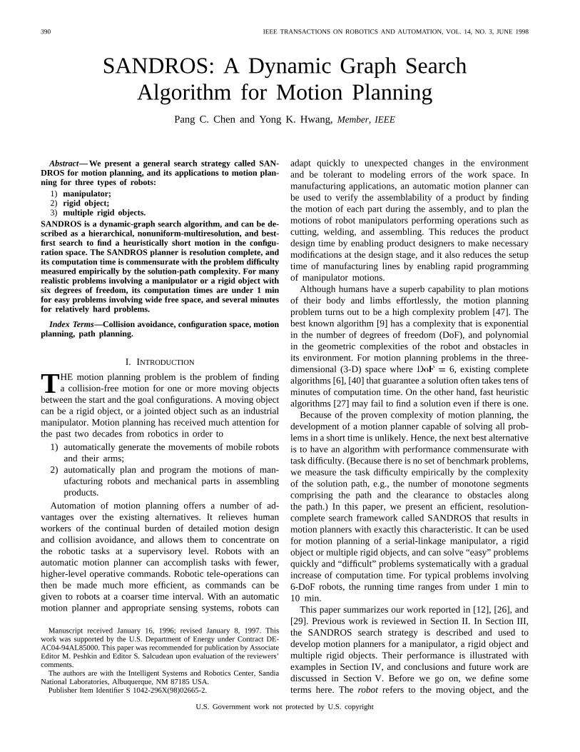
Fig. 1. Sequence verification and node refinement.

when either the entire sequence is connected, or a nodeisfound unreachable from a point. In the former, we wouldretrace a path from to through to yield a motion for therobot. In the latter, however, we would disconnectfrom ,push both and into if they are not in already, andreturn to generating another sequence.

4) Node Refinement:Continuing with the sequence gener-ation process, if the graph algorithm produces no candidatesequence, then we would enter the node refinement stage. Inthis stage, we modify continually by refining the subgoalsin until either a candidate sequence becomes available, orbecomes empty. We pop off every nodein deemed to havethe least amount of refinement and refine it into more clear,defined subgoals. After refininginto children , the nextstep is to modify to reflect the change in . We augment

with by inserting into , and connecting everyneighbor node of with every node of while observingappropriate edge constraints (described in the next section).Also, if has not been refined already, then we wouldpush into to ensure the eventual chance that everynode of gets refined.

Fig. 1 illustrates the sequence verification and refinementusing rectangular subgoals. Fig. 1(a) shows a refinement of theC-space into subgoals, and a test sequence is shown in boldrectangles. Fig. 1(b) showsfinding a collision-free path fromone subgoal to the next, till the goal is reached (bidirectionalsearch not shown for simplicity). If all sequences fail togenerate a solution, and if nodeis chosen for refinement,several new sequences become available for verification by[Fig. 1(c)].

B. Node Representation and Refinement

Although subgoal representation is independent of thesearch framework thus presented, it is nevertheless animportant factor in determining the efficiency of the eventualsearch. For manipulators and rigid bodies, we find thefollowing two approaches to be quite effective.

1) Manipulators: For a manipulator (single open kinematicchain) with DoF a node at (refinement) level is a -vector with only the first components specified, which is anaffine space of dimension . Thus, the totally unspecifiednode at level 0 represents the entire C-space, and a fullyspecified node represents a single point. The edge cost between

two nodes is defined as the sum of the differences betweenthe coordinates that are specified in both nodes (a modifiedManhattan metric). Nodes are connected by an edge only ifthe edge cost does not exceed a certain threshold.

In the node refinement stage, nodes at the highest level arerefined: A node at level is refined as follows: First, weuse the specified components ofas the first joint valuesfor the robot. Then, using only the links whose positions aretotally specifiable by the first 1 joints, we compute thedistance between the links and other objects in the work spacefor all possible ( 1)th joint values at a prescribed resolutioncalled stride (see Section III-C). The resulting set of nodeswith 1 specified components and positive distance is thenfiltered into a list of nodes using adominate-and-killmethod. In this method, the process of selecting a nodewith the maximum distance value, and removing each nodewhose ( 1)th component is within number of nodes of

is repeated until every node is considered. The idea is tocondense the set of possible nodes into a sparse collection ofsubgoals having maximal clearances based on the specifiedlinks. Refinement stops when all nodes are fully specified.

2) Rigid Bodies: For a rigid object, a node is simply arectilinear cell of the C-space. That is, for each dimension, alow and high value specify the range of valid configurations.Together, the nodes form a partition of the C-space. Two nodesare connected with an edge if they are adjacent in that theircontact area is nonzero. The edge cost between two nodes isdefined as the Euclidean distance between the centers of thetwo cells. In the node refinement stage, nodes with the largestvolume, are refined by cutting on the longest side in half. Thatis, the nodes that contain the most number of lattice points inthe discretized C-space are split in half along the dimensioncontaining the most number of lattice points. Refinement stopswhen the longest side of the nodes contains only one latticepoint. For multiple objects, the C-space is the product of theC-spaces of all objects. The form of node, edge and edge costare similarly defined as for the case of a single rigid object.

C. Local Planning

The local planner simulates robot movements in the C-spacein small steps. A step is defined as a configuration changewhere a DoF is changed by a preset amount calledstride,which represents the resolution. The stride in each dimension


is normalized so that the maximum distance traveled by anypoint on the robot is about the same for each stride. A pointthat is within one step of another is a neighbor of that point.Collision checking is done after the robot takes a step. It ispossible for the robot to collide with the objects during a step,although it does not before and after the step. The Jacobianmethod [45] can be used to dynamically control the stride sizesand ensure no inter-step collisions, but we have decided to usesmall fixed strides for implementation efficiency.

The local planner checks the reachability of a nodefrom a point by moving the robot from to any point in

. If is found, then the cost of is recursively defined asthe cost of plus the number of steps needed to move from

to . The iterative procedure of moving fromtoward isas follows: First, we make progress towardby consideringall neighboring points of that are one step closer tothan is, and move to the point that has the maximumclearance 0. (Whether the node is an affine space ora cuboid, the distance between pointand node is definedas the minimum Euclidean distance betweenand , which iseasily computed.) Next, we “slide” repeatedly by consideringsequentially in each dimension, the two neighboring points onestep away in either direction. If there is a point closer to

than is, while having a larger clearance , we wouldmove from to and set to . If no progress can bemade, then would report a failure; otherwise, the move-toward-and-slide procedure is repeated untilis reached.

D. Post Processing of Path and Optimality

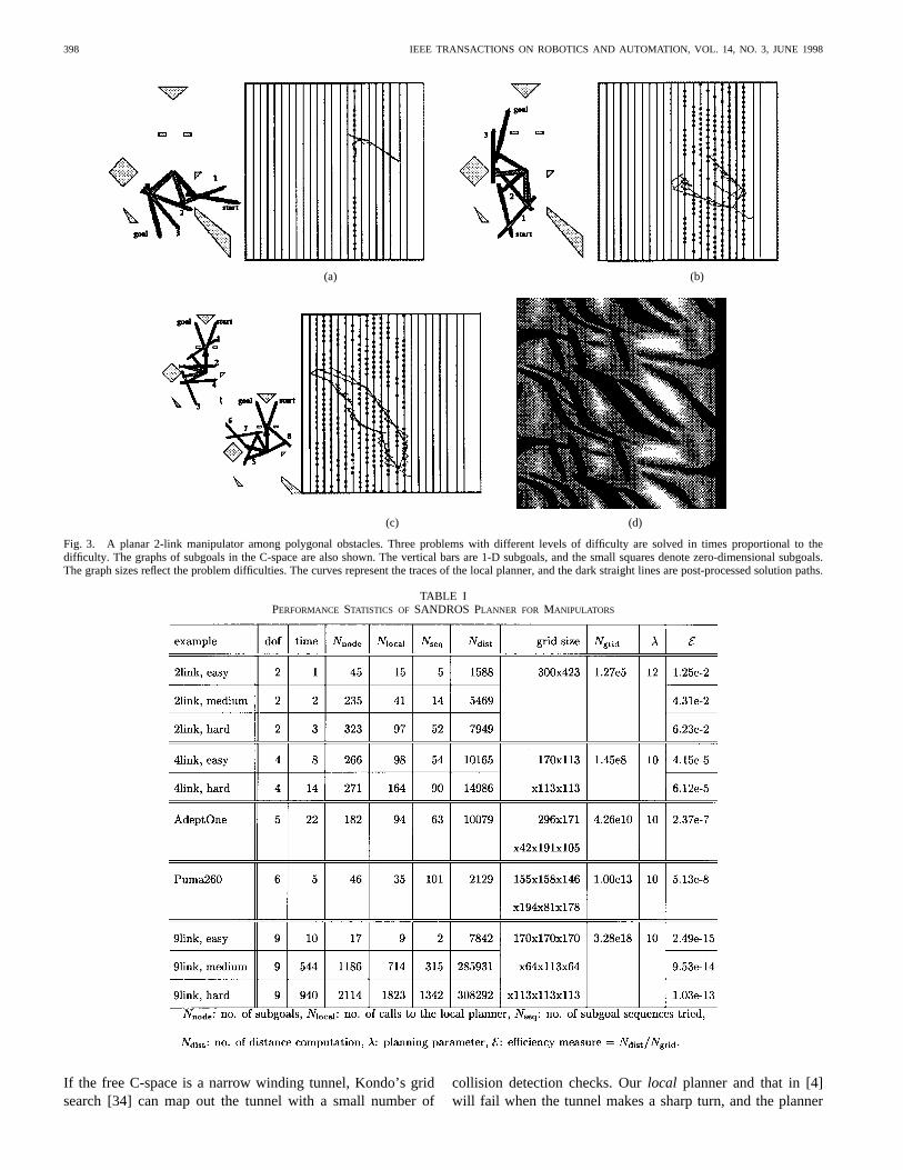
A solution path found typically has many noise-like kinkssince tries maximize obstacle distance as much as possiblewhile moving toward the goal. To locally optimize the path,we have developed a method calledcorner-cut. It deletesevery other points of the solution path, and tests if the robotcan move between the remaining points by interpolation. Ifa collision occurs during interpolated movement between twopoints, the deleted path point between them is re-inserted to thepath. This process of deleting every other point and checkingcollision via interpolation is repeated until no more point canbe deleted. The C-spaces in Fig. 3 show the original wigglypaths and the corner-cut paths consisting of a small numberof line segments. A corner-cut path can be further optimizedusing numerical methods that minimizes a weighted sum ofpath length, distance to obstacles along the path and othermeasures [27], [45].

The near-optimality of the path found by our algorithm issupported only qualitatively and empirically. Because SAN-DROS verifies a node sequence with the smallest cost, a shortpath is heuristically more likely to be found first than a longerpath. Grossly nonoptimal paths are of two types.

1) First, the solution path is found from a sequence of largesubgoals. This happens when the free space is wide,but there are enough obstacles to make the robot take adetour. This type of paths can be made near-optimal withrespect to homotopy by post-processing in most cases.

2) Second, the solution found and the optimal path are ondifferent sides of an obstacle. The only way to overcome

this problem is to continue to search the C-space untila satisfactory solution is found. Note that it is hardto define what is satisfactory and know when to stopsearching.

For practicality, one probably has to be content with stoppingwhen the difference of path lengths of two successive solutionsbecomes small, or no more solution is found within a presettime limit.

E. Completeness Proof

To recapitulate, our algorithm searches for a solution byrepeating the process of finding a promising sequence ofnodes in a graph , verifying its feasibility with , andmodifying with the refinement procedure. The efficiencyof our algorithm comes from the fact that we delay the noderefinement until there is no candidate sequence available at thecurrent refinement level ( disconnected). Such delay allowsus to find a solution quickly in a graph with only a small butrepresentative set of subgoals when intricate maneuvering isnot needed.

It is of course possible to refine completely every node ofdown to a point first, and then plan a path based on the

resulting unique network of points . However, it would beterribly inefficient to find the shortest plausible sequence ofsubgoals because of the sheer size of. In fact, for rigidbodies, the resulting network is simply the discretized mapof the free C-space, and only needs to check whether anadjacent point is collision-free. On the other hand, using anontrivial refinement parameter for manipulators allows usto combine similar subgoals into one single subgoal and utilizethe power of to connect subgoals that areaway from eachother.

For manipulators, there’s no guarantee of finding a solutionin a with a nontrivial when one exists in the corresponding

with 0. The same lack of guarantee goes for rigidbodies, if we choose not to refine nodes down to the resolution.(Users who fear that there’s no solution may wish to do soto reduce the amount of time wasted.) However, for bothmanipulators and rigid bodies, we can show that if a solutionexists in , then SANDROS will also find one in withoutnecessarily refining every node down to a point.

Theorem 1: Suppose that a task of moving fromto issolvable by first refining the C-space into a network of points

, and then planning a path throughusing to connectto . Then our algorithm is complete in that it can also solvethe same problem, but with possibly less node refinement.

Proof: If the problem of moving from to is solv-able through total refinement, then there must be a looplesssequence withsuch that is able to connect with for all .Suppose that our algorithm fails to solve the same problem,and terminates with a partially refined . Then considerthe sequence where denotesthe node of that dominates in that the subspace ofcontains that of . By contracting any loop of this sequencerepeatedly, and then picking the subsequence starting withthe last point in and ending with the first point in ,


we can obtain a loopless (but not unique) sequence of theform with , andeach in . Since contains no repetition of nodes andhas a finite cost (because the cost of is finite), it mustbe a sequence verified by to be infeasible. Because isloopless, every fully refined node in must correspondto a unique in . Further, for such mustdominate . Hence, for to be infeasible, there mustexist a smallest 1 such that strictly dominates inthat is still not fully refined. On the other hand, suchcannot exist for the following reason. If were reachableby the end of our algorithm, then would eventually bepushed into . (See the last portion of Section III-A.) Ifwere not reachable, then would have been pushed intoimmediately after this determination. Either way, wouldhave been expanded eventually and totally, and hence cannotstrictly dominate . Therefore, our algorithm must have alsosucceeded by contradiction.

Thus, we have the guarantee that while minimizing thenumber of nodes in , SANDROS’ interleaving process ofsearch and refinement will eventually find a solution if thereis a solution in the completely refined graph.

IV. EXAMPLES

SANDROS search strategy has been applied to motionplanning of a manipulator, a rigid object, and multiple rigidobjects. SANDROS planner is run on both easy and hardproblems, and its performance is illustrated using the followingnumbers. The computation times are run times on a 200MHz SGI Indigo2 workstation. The number of nodes on thegraph generated by SANDROS, the number of calls to thelocal planner and the number of distance computations giveempirical ideas of the problem difficulty. We used the distanceroutine in [19] developed for polyhedral objects, and thus robotand obstacle shapes are polyhedral.

To get a meaningful and fair assessment of SANDROS’efficiency, the following measure is developed.

1) First, we use the number of collision detection (ordistance) computations between the robot and its en-vironment rather than computation time, since it isindependent of geometric complexities of the robot andobstacles.

2) Second, SANDROS’ efficiency is compared against abrute-force grid-search method in the C-space, whichdiscretizes the C-space into points, performs col-lision detection at each point, and finds a path amongthe collision-free points.

This planner will run in time. Let be thelength of the C-space in theth dimension. Then

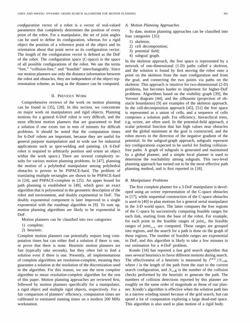
stride . The SANDROS’ efficiency, , is thenmeasured by the ratio of , the number of distancecomputations by SANDROS, to the of the C-spacegrid. (If we used stride , then wewould have measured the efficiency of interleaving searchwith subgoal refinement against performing search after totalrefinement within SANDROS’ framework.)

Fig. 2. Ratio of the number of collision-check points to the total numberof points in the C-space, plotted in log scale against the degrees of freedomof the robot(s).

In Fig. 2, for the examples that followare plotted in log scale against DoF, and this empiricallyshows the efficiency of our algorithm for high-DoF problems.The apparent “log-linearity” exhibited in the plot indicates anexponential time improvement of SANDROS over the trivialplanner, even though SANDROS’ performance may still beexponential in DoF.

Tables I–III shows detailed statistics on examples: the num-ber of DoF, computation times, number of nodes in the graph,number of local planner invoked, number of subgoal sequencestried, number of distance computations, C-space grid size,search parameter, and . The most important parametersof our planner are the strides, and . The strides usedare typically 2–5 for rotation, and can be inferred by thegrid size in the tables. The stride should be set so that at allpoints on the solution path the robot should be able to move atleast one step along each dimension of the C-space. This willallow the local planner rooms to slide around obstacles. Formanipulators, denotes the distance between subgoals. Thelarger it is, the faster the planner runs and the bigger the chanceof not finding a solution. The value of ten seems to achievethe most efficiency without causing failures in our examples.The maximum distance between neighbor nodes, 1.5

in all examples. For single or multiple rigid objects1 is used, but all examples were solved before the lengths ofcuboid subgoals reach stride. For practical applications, werecommend using another parameter such that the localplanner executes the sliding strategy only when the distance toobstacles is less than , which is set to in our examples.

We compare the performance of our planner with only thosewhich make point queries to check collision or to computedistance, since an objective comparison is hard to do withdifferent approaches. The average efficiency of our plannermeasured by the number of distance computations is roughlyon the same order of magnitude as those of the planners in[4], [23], and [34]. If we are solving five to ten differentproblems in the same environment, the planner in [31] isequally efficient. Their performance depends on the problem.


(a) (b)

(c) (d)

Fig. 3. A planar 2-link manipulator among polygonal obstacles. Three problems with different levels of difficulty are solved in times proportional tothedifficulty. The graphs of subgoals in the C-space are also shown. The vertical bars are 1-D subgoals, and the small squares denote zero-dimensional subgoals.The graph sizes reflect the problem difficulties. The curves represent the traces of the local planner, and the dark straight lines are post-processed solution paths.

TABLE IPERFORMANCE STATISTICS OF SANDROS PLANNER FOR MANIPULATORS

If the free C-space is a narrow winding tunnel, Kondo’s gridsearch [34] can map out the tunnel with a small number of

collision detection checks. Ourlocal planner and that in [4]will fail when the tunnel makes a sharp turn, and the planner


TABLE IIPERFORMANCE STATISTICS OF SANDROS PLANNER FOR RIGID OBJECTS

TABLE IIIPERFORMANCE STATISTICS OF SANDROS PLANNER FOR MULTIPLE RIGID OBJECTS

in [31] will take a long time to find a feasible configurationin the tunnel via random sampling.

If the C-space has a big dead-end space, i.e., a trap, andthe robot has to backtrack, Kondo’s algorithm is somewhatinefficient due to the lack of anexplicit backtracking mecha-nism. Our planner and the planners in [23] and [31] providebacktracking mechanisms with subgoals, visibility graph orraodmap, respectively, and can better handle traps. Our plannerand that in [23], however, do not generalize well for amanipulator with a tree structure, but the planners in [4],[31], and [34] have no problem. For a general application,the best way is to run all of these in parallel and take the firstsatisfactory solution.

A. Manipulator

Fig. 3 shows three problems of increasing difficulty with a2-link planar robot. Solution motions and the subgoal graphsin the C-space are shown along with the C-space obstacles[Fig. 3(d)]. The size of the subgoal graph increases withthe problem difficulty. The real power of SANDROS shows

Fig. 4. Two 4-DoF problems solved in 8 s (left) and 14 s (right).

in solving problems with higher DoFs. Fig. 4 shows 4-DoFproblems, which are solved in 8 and 14 s. Planning motionof a 5-DoF AdeptOne robot to move an L shape out of awicket to the left side of the table takes 22 s (Fig. 5). Pullinga stick from behind two vertical posts with a 6-DoF Pumarobot is shown in Fig. 6 (5 s). Finally, the 9-DoF problemshown in Fig. 7(c) takes about 15 min, showing the gradual


Fig. 5. A 5-DoF Adept robot is moving an L-shaped object out of a wicketand places it on the left side of the table. The computation time is 22 s.

Fig. 6. The SANDROS planner took 5 s to find the motion to move a stickthrough the two vertical posts.

Fig. 7. Easy, intermediate, and hard problems involving a nine-link planarrobot. It took SANDROS 10 s (top left), 10 min (top right) and 16 min(bottom) to solve these problems, respectively.

increase of computation time with DoF. In the examples abovewhere obstacles and robots have about ten to 40 faces, thetime for one distance computation was roughly 1 ms. Fortypical 5 and 6-DoF problems of moderate difficulty (Figs. 5and 6), SANDROS shows near real-time performance. If thegeometric complexities of robots and environments increase,or for very difficult problems, SANDROS will need a 10 to100 times faster computer for near real-time performance.

Fig. 8. Moving an L shape. SANDROS took 1 s to solve this problem.

Fig. 9. Unhooking a paper clip from a nail (small square). The computationtime is 1 s. The rectangular partition shows subgoals generated by SANDROS.

(a) (b)

Fig. 10. Moving a paper clip away from two nails (small squares) took 8 sfor SANDROS. The cell subgoals and the traces of the local planner areshown in (b).

Fig. 11. Moving an L shape around the corner of a hallway (front walls notshown). It took one call to the local planner to solve this problem.

B. Rigid Object

Fig. 8 shows a simple 2-D problem, solved in 1 s. Fig. 9shows the problem of unhooking a half-open paper clipfrom a nail (small square). The partition of the space intorectangles shows the cell-subgoals used by SANDROS. Whenwe add another nail, the problem becomes considerably harder,and Fig. 10(b) shows a more complex partition of C-spacecomputed by SANDROS. Fig. 11 shows how to move an L


Fig. 12. Moving a T shape out of a jail. The computation time is 6 s.

Fig. 13. Moving a Pi shape out a jail. The computation time is 89 s.

Fig. 14. Two people exchanging their positions in a small room. This 6-DoFproblem was solved in 6 s.

abound the corner of a hallway (front walls not shown). Itturns out that SANDROS can solve this problem with just onecall to the local planner. Figs. 12 and 13 show how to move aT and a Pi shapes out of a jail cell (6 and 89 s). Note that real-world problems do not get much harder than these problems.Otherwise, the robot should probably remove some obstacles.

C. Multiple Rigid Objects

For multiple movers’ problem, SANDROS is most usefulwhen the total DoF of robots is not too large (13) andthe solution requires simultaneous motions of robots. If robotscan be moved one at a time, it is better to decompose theproblem into a sequence of single mover’s problems. Fig. 14shows the top view of two people exchanging their positionsin a small room (6 s). The spike example in Fig. 15 is takenfrom [43] which was used to show that there is an assemblyrequiring an arbitrarily many hands to assemble. (We addeda finite tolerance between the baseboard and the spikes sinceour planner considers contacts as collisions.) A nonmonotone

Fig. 15. An assembly requiring simultaneous movements of three objects.This 9-DoF problem was solved in 6 s.

(a) (b)

Fig. 16. This nonmonotone assembly needs the crucial configuration in (b)to be assembled. It is solved in 4 s with only translation (4 DoF), and in 82 swhen rotation is also allowed (6 DoF).

(a) (b)

Fig. 17. (a) Moving six mobile robots to the opposite side of the room. Thecomputation time is 207 s. (b) Snapshot at a point along the solution path.

assembly problem of inserting two parts in Fig. 16(a) is solvedin 4 s when only translational motion is allowed (4 DoF). Ifthe rotation is included (6 DoF problem), it is solved in 82 s,most of time being spent on finding the crucial configurationin Fig. 16(b).

Fig. 17 shows six mobile robots trying to go to the oppositeside of a room (an 18-DoF problem, 207 s). Fig. 17(b) showsa snap shot of the room at one point of the solution motion.The motions are erratic since the planner tries to move themaway from one another. The problems of rearranging two andthree pieces of furniture in 3-D are shown in Figs. 18 (2 min)and 19 (7.5 h).

V. CONCLUSION

We have presented a dynamic graph search algorithm calledSANDROS, and applied it to the gross motion planning ofa manipulator, a rigid object, and multiple rigid objects. Itis a resolution-complete algorithm with computation time


Fig. 18. Rearranging two pieces of furniture (the ceiling and the front wallare not shown). It took SANDROS 2 min to solve this 12-DoF problem.

(a) (b) (c)

(d) (e) (f)

Fig. 19. Rearranging three pieces of furniture (the ceiling and the front wallare not shown). It took SANDROS 7.5 h to solve this 18-DoF problem.

commensurate with problem difficulty, and is one of the mostefficient and complete motion planners developed to date.SANDROS algorithm is a judicious combination of severalimportant ideas developed in motion planning over the pastdecade. They are multiresolution search using hierarchicalcell division of the C-space [7], a local planner based on apotential field [32], [27], a two-level search scheme in [18],sequential computation of collision-free joint-angle ranges fora manipulator [40], an efficient distance computation [19], anda bidirectional search [27]. To obtain a planner significantlyfaster than ours would seem to require using massively parallelmachines [10], or taking a totally different approach utilizingsensors or additional knowledge.

SANDROS planner has many applications. For manipu-lators, it can be usedon-line in unstructured environmentssuch as in exploration or waste-site cleanup. For structuredenvironments such as in manufacturing, it can automaticallyprogram robotsoff-line in place of manual programming. Ourplanner for a rigid object can be used for navigating mobilerobots, and to plan motions to assemble mechanical products.Our planner for multiple rigid objects is especially useful forcases where simultaneous motions of robots are required. Ourplanners show the best performance when there are less than10 DoF. For low-DoF problems, brute-force algorithms alsoperform well, while for problems with many DoF (e.g.,10),the algorithms in [4] and [42] are more suitable.

There are many future directions in motion planning re-search. For the model-based approach, planning motions withcontacts will benefit assembly planning research. Polyhedralconvex cones [21] are the most popular tool for this. Forthe sensor-based approach, selectively building models of theenvironment at the right resolution will be a good researchdirection. Purely sensor-based algorithms will be suitablefor reflex motions, while some model of the world will

be necessary for global planning [41]. Developing a fasterdistance routine can reduce motion planning time even further.For example, the thresholded distance [52] does not computethe exact distance if it determines the distance is greater thana threshold, and thereby reducing the computation time. Sincethe collision avoidance need not be done unless obstaclesare closer than some threshold ( in Section IV, fourthparagraph), the thresholded distance is particularly useful formotion planning.

Constraints such as nonholonomic constraints can be incor-porated into motion planning by constraining robot motion inthe local planner [48]. To include dynamics, the search hasto be done in the position-velocity space, or the phase space[15]. The knowledge-based approach for motion planning isexplored to some extent. For example, spatial reasoning is in-corporated into motion planning in [30]. Issues like knowledgerepresentation and plan generation must be resolved before aknowledge-based motion planner can be developed.

ACKNOWLEDGMENT

The authors would like to thank E. G. Gilbert, University ofMichigan, for providing the software for computing distancebetween polyhedra, and the reviewers of this paper, includingD. R. Strip, R. C. Brost, and P. G. Xavier.

REFERENCES

[1] A. Aho, J. Hopcroft, and J. Ullman,The Design and Analysis ofComputer Algorithms. Reading, MA: Addison-Wesley, 1974.

[2] F. Avnaim, J. D. Boissonnat, and B. Faverjon, “A practical exact motionplanning algorithm for polygonal objects amidst polygonal obstacles,”in Proc. IEEE Int. Conf. Robot. Automat., Philadelphia, PA, 1988, pp.1656–1661.

[3] J. Barraquand and P. Ferbach, “Path planning through variationaldynamic programming,” inProc. IEEE Int. Conf. Robot. Automat., SanDiego, CA, 1994, pp. 1839–1846.

[4] J. Barraquand and J. C. Latombe, “A Monte-Carlo algorithm for pathplanning with many degrees of freedom,” inProc. IEEE Int. Conf. Robot.Automat., Cincinnati, OH, 1990, pp. 1712–1717.

[5] , “Robot motion planning: A distributed representation approach,”Int. J. Robot. Res., vol. 10, pp. 628–649, 1991.

[6] P. Bessiere, J.-M. Ahuactzin, E.-G. Talbi, and E. Mazer, “The “Ariadne’sClew” algorithm: Global planning with local method,” inProc. Int. Conf.Intell. Robot. Syst., 1993, pp. 1373–1380.

[7] R. A. Brooks and T. Lozano-Perez, “A subdivision algorithm in config-uration space for findpath with rotation,”Int. Joint Conf. Artif. Intell.,Karlsruhe, Germany, 1983.

[8] S. J. Buckley, “Fast motion planning for multiple moving robots,”in Proc. IEEE Int. Conf. Robot. Automat., Scottsdale, AZ, 1989, pp.322–326.

[9] J. F. Canny,The Complexity of Robot Motion Planning. Cambridge,MA: MIT Press, 1988.

[10] D. Challou, M. Gini, V. Kumar, and C. Olson, “Very fast motionplanning for dexterous robots,” inProc. IEEE Int. Symp. Assembly TaskPlan, Pittsburgh, PA, 1995, pp. 201–206.

[11] P. C. Chen, “Improving path planning with learning,” inProc. 9th Int.Conf. Mach. Learn, 1992, pp. 55–61.

[12] P. C. Chen and Y. K. Hwang, “SANDROS: A motion planner withperformance proportional to task difficulty,” inProc. IEEE Int. Conf.Robot. Automat., Nice, France, 1992, pp. 2346–2353.

[13] Y. K. Hwang and P. C. Chen, “A heuristic and complete planner for theclassical mover’s problem,” inProc. IEEE Int. Conf. Robot. Automat.,Nagoya, Japan, May 1995, pp. 729–736.

[14] B. Donald, “Motion planning with six degrees of freedom,” tech. rep.AI-TR-791, Arti. Intell. Lab., Mass. Inst. Technol., Cambridge, MA,1984.

[15] B. Donald, P. Xavier, J. Canny, and J. Reif, “Kinodynamic motionplanning,” J. ACM, vol. 40, no. 5, pp. 1048–1066, Nov. 1993.


[16] M. Erdmann and T. Lozano-Perez, “On multiple moving objects,” inProc. IEEE Int. Conf. Robot. Automat., San Francisco, CA, 1986, pp.1419–1424.

[17] B. Faverjon, “Obstacle avoidance using an octree in the configurationspace,” inProc. IEEE Int. Conf. Robot. Automat., Atlanta, GA, Mar.1984, pp. 1152–1159.

[18] B. Faverjon and P. Tournassoud, “A local approach for path planning ofmanipulators with a high number of degrees of freedom,” inProc. IEEEInt. Conf. Robot. Automat., Raleigh, NC, Mar. 1987, pp. 1152–1159.

[19] E. G. Gilbert, D. W. Johnson, and S. S. Keerthi, “A fast procedure forcomputing the distance between complex objects in three-dimensionalspace,”IEEE J. Robot. Automat., vol. 4, pp. 193–203, Apr. 1988.

[20] A. J. Goldman and A. W. Tucker, “Solving findpath by combination ofgoal-directed and randomized search,” inProc. IEEE Int. Conf. Robot.Automat., Cincinnati, OH, May 1990, pp. 1718–1723.

[21] , “Polyhedral convex cones,” inLinear Inequalities and RelatedSystems, Annals of Mathematics Studies 38, H. W. Kuhn and A. W.Tucker, Eds. Princeton, NJ: Princeton Univ. Press, pp. 19–39.

[22] K. K. Gupta, “Fast collision avoidance for manipulator arms: A se-quential search strategy,” inProc. IEEE Int. Conf. Robot. Automat.,Cincinnati, OH, May 1990, pp. 1724–1729.

[23] , “A 7-DoF practical motion planner based on sequential frame-work: Theory and experiments,” inProc. IEEE Int. Symp. Assem. TaskPlan., Pittsburgh, PA, 1995, pp. 213–218.

[24] J. Hopcroft, D. Joseph, and S. Whiteside, “Movement problems for 2-dimensional linkages,”SIAM J. Comput., vol. 13, no. 3, pp. 610–629,1984.

[25] J. Hopcroft and G. T. Wilfong, “Reducing multiple object motionplanning to graph searching,”SIAM J. Comput., vol. 15, no. 3, pp.768–785, 1986.

[26] Y. K. Hwang, “Motion planning for multiple moving objects,” inProc.IEEE Int. Symp. Assem. Task Plan, Pittsburgh, PA, 1995, pp. 400–405.

[27] Y. K. Hwang and N. Ahuja, “Potential field approach to path planning,”IEEE Trans. Robot. Automat., vol. 8, pp. 23–32, Feb. 1992.

[28] , “Gross motion planning—A survey,”ACM Comput. Surv., vol.24, no. 3, pp. 219–292, Sept. 1992.

[29] Y. K. Hwang and P. C. Chen, “A heuristic and complete planner for theclassical mover’s problem,” inProc. IEEE Int. Conf. Robot. Automat.,Nagoya, Japan, May 1995, pp. 729–736.

[30] Y. K. Hwang, P. C. Chen, and P. A. Watterberg, “Interactive taskplanning through natural language,” inProc. IEEE Int. Conf. Robot.Automat., Minneapolis, MN, May 1995, pp. 24–29.

[31] L. Kavraki, P. Svestka, J.-C. Latombe, and M. H. Overmars, “Prob-abilistic roadmap for path planning in high dimensional configurationspace,”IEEE Trans. Robot. Automat., vol. 12, pp. 566–580, Aug. 1996.

[32] O. Khatib, “Real-time obstacle avoidance for manipulators and mobilerobots,” inProc. IEEE Int. Conf. Robot. Automat., St. Louis, MO, 1985,pp. 500–505.

[33] Y. L. Koga and J. C. Latombe, “On multi-arm manipulation planning,”in Proc. IEEE Int. Conf. Robot. Automat., San Diego, CA, 1994, pp.945–952.

[34] K. Kondo, “Motion planning with six degrees of freedom by multistrate-gic bidirectional heuristic free-space enumeration,”IEEE Trans. Robot.Automat., vol. 7, pp. 267–277, June 1991.

[35] J. C. Latombe,Robot Motion Planning. New York: Kluwer, 1991.[36] S. M. LaValle and S. A. Hutchinson, “Path selection and coordination

for multiple robots via Nash equilibria,” inProc. IEEE Int. Conf. Robot.Automat., San Diego, CA, 1994, pp. 1847–1852.

[37] J. Lengyel, M. Reichert, B. R. Donald, and D. P. Greenberg, “Real-timerobot motion planning using rasterizing computer graphics hardware,”Comput. Graph., vol. 24, no. 4, pp. 327–335, Aug. 1990.

[38] Y. H. Liu, S. Kuroda, T. Naniwa, H. Noborio, and S. Arimoto, “Apractical algorithm for planning collision-free coordinated motion ofmultiple mobile robots,” inProc. IEEE Int. Conf. Robot. Automat.,Scottsdale, AZ, 1989, pp. 1427–1432.

[39] T. Lozano-Perez and M. A. Wesley, “An algorithm for planningcollision-free paths among polyhedral obstacles,”Commun. ACM, vol.22, no. 10, pp. 560–570, 1979.

[40] T. Lozano-Perez, “A simple motion-planning algorithm for general robotmanipulators,”IEEE J. Robot. Automat., vol. RA-3, pp. 224–238, June1987.

[41] V. J. Lumelsky, “Incorporating body dynamics into the sensor-basedmotion planning paradigm, the maximum turn strategy,” inProc. IEEEInt. Conf. Robot. Automat., Nagoya, Japan, 1995, pp. 1637–1642.

[42] A. A. Maciejewski and C. A. Klein, “Obstacle avoidance for kinemat-ically redundant manipulators in dynamically varying environments,”Int. J. Robot. Res., vol. 4, no. 3, pp. 109–117, 1985.

[43] B. K. Natarajan, “On planning assemblies,” inProc. 4th ACM Symp.Computat. Geometry, 1988, pp. 299–308.

[44] C. O’Dunlaing and C. K. Yap, “A retraction method for planning themotion of of a disc,”J. Algorithms, vol. 6, pp. 104–111, 1982.

[45] B. Paden, A. Mees, and M. Fisher, “Path planning using a Jacobian-based freespace generation algorithm,” inProc. IEEE Int. Conf. Robot.Automat., Scottsdale, AZ, 1989, pp. 1732–1737.

[46] C. Qin, S. Cameron, and A. McLean, “Toward efficient motion planningfor manipulators with complex geometry,” inProc. IEEE Int. Symp.Assem. Task Plan, Pittsburgh, PA, 1995, pp. 207–212.

[47] J. H. Reif, “Complexity of the mover’s problem and generalizations,” inProc. 20th IEEE Symp. Foundations Comput. Sci., 1979, pp. 421–427.

[48] P. Svestka and M. H. Overmars, “Coordinated motion planning formultiple car-like robots using probabilistic road maps,” inProc. IEEEInt. Conf. Robot. Automat., Nagoya, Japan, May 1995, pp. 1631–1636.

[49] J. T. Schwartz and M. Sharir, “On the piano movers’ problem: II. Tech-niques for computing topological properties of real algebraic manifolds,”Advances in Applied Mathematics. New York: Academic, 1983, pp.298–351.

[50] R. H. Wilson and T. Matsui, “Partitioning an assembly for infinitesimalmotions in translation and rotation,” inProc. Int. Conf. Intell. RobotsSyst., 1992, pp. 1311–1318.

[51] C. K. Yap, “How to move a chair through a door,”IEEE J. Robot.Automat., vol. RA-3, pp. 172–181, 1987.

[52] P. A. Watterberg, P. G. Xavier, and Y. K. Hwang, “Path planning foreveryday robotics with SANDROS,” inProc. IEEE Int. Conf. Robot.Automat., Albuquerque, NM, 1997, pp. 1171–1176.

[53] D. Y. Yeung and G. A. Bekey, “A decentralized approach to the motionplanning problem for multiple mobile robots,” inProc. IEEE Int. Conf.Robot. Automat., Raleigh, NC, 1987, pp. 1779–1784.

Pang C. Chenreceived the Ph.D. degree in com-puter science from Stanford University, Stanford,CA, in 1989.

He presently works at the Sandia National Lab-oratories, Albuquerque, NM. His research interestsinclude combinatorial algorithms, machine learning,and massively parallel computing. His personal life-long challenge is to develop a Go-playing programthat can defeat him using AI techniques and dis-tributed computing resources.

Dr. Chen is a co-recipient of the 1994 Research& Development 100 Award for his work on motion planning.

Yong K. Hwang (M’87) received the Ph.D. degreein electrical engineering from the University ofIllinois, Urbana-Champaign, in 1988.

Since then, he has been working at the SandiaNational Laboratories, Albuquerque, NM, and iscurrently a Principal Member of Technical Staff. Hisresearch interests include robotics, vision, artificialintelligence, and man-machine interface.

Dr. Hwang is a co-recipient of the 1994 Research& Development 100 Award for his work on motionplanning.

sandros: a dynamic graph search algorithm for …amato/courses/689/papers/sandros_ra_t… · 390...

Documents