sarah blunt, jason wang, henry ngo, et al
TRANSCRIPT
orbitize Documentation
Sarah Blunt, Jason Wang, Henry Ngo, et al.
Jan 19, 2022

CONTENTS
1 Attribution: 3
2 User Guide: 52.1 Installation . . . . . . . . . . . . . . . . . . . . . . . . . . . . . . . . . . . . . . . . . . . . . . . . 52.2 Tutorials . . . . . . . . . . . . . . . . . . . . . . . . . . . . . . . . . . . . . . . . . . . . . . . . . 62.3 Frequently Asked Questions . . . . . . . . . . . . . . . . . . . . . . . . . . . . . . . . . . . . . . . 952.4 Contributing to the Code . . . . . . . . . . . . . . . . . . . . . . . . . . . . . . . . . . . . . . . . . 1012.5 Detailed API Documentation . . . . . . . . . . . . . . . . . . . . . . . . . . . . . . . . . . . . . . 101
3 Changelog: 133
Python Module Index 139
Index 141
i

ii
orbitize Documentation
Hello world! Welcome to the documentation for orbitize, a Python package for fitting orbits of directly imagedplanets.
orbitize packages two back-end algorithms into a consistent API. It’s written to be fast, extensible, and easy-to-use.The tutorials below will walk you through the code and introduce some technical stuff, but we suggest learning about theOrbits for the Impatient (OFTI) algorithm and MCMC algorithms (we use this one) before diving in. Our contributorguidelines document will point you to more useful resources.
orbitize is designed to meet the needs of the exoplanet imaging community, and we encourage community involve-ment. If you find a bug, want to request a feature, etc. please create an issue on GitHub.
orbitize is patterned after and inspired by radvel.
CONTENTS 1

orbitize Documentation
2 CONTENTS
CHAPTER
ONE
ATTRIBUTION:
• If you use orbitize in your work, please cite Blunt et al (2019).
• If you use the OFTI algorithm, please also cite Blunt et al (2017).
• If you use the Affine-invariant MCMC algorithm from emcee, please also cite Foreman-Mackey et al (2013).
• If you use the parallel-tempered Affine-invariant MCMC algorithm from ptemcee, please also cite Vousden etal (2016).
• If you use the Hipparcos intermediate astrometric data (IAD) fitting capability, please also cite Nielsen et al(2020) and van Leeuwen et al (2007).
• If you use Gaia data, please also cite Gaia Collaboration et al (2018; for DR2), or Gaia Collaboration et al (2021;for eDR3).
3

orbitize Documentation
4 Chapter 1. Attribution:
CHAPTER
TWO
USER GUIDE:
2.1 Installation
2.1.1 For Users
Parts of orbitize are written in C, so you’ll need gcc (a C compiler) to install properly. Most Linux and Windowscomputers come with gcc built in, but Mac computers don’t. If you haven’t before, you’ll need to download Xcodecommand line tools. There are several helpful guides online that teach you how to do this. Let us know if you havetrouble!
orbitize is registered on pip, and works in Python>3.6. To install orbitize, first make sure you have the latestversions of numpy and cython installed. With pip, you can do this with the command:
$ pip install numpy cython --upgrade
Next, install orbitize:
$ pip install orbitize
We recommend installing and running orbitize in a conda virtual environment. Install anaconda or minicondahere, then see instructions here to learn more about conda virtual environments.
2.1.2 For Windows Users
Many of the packages that we use in orbitize were originally written for Linux or macOS. For that reason, we highlyrecommend installing the Windows Subsystem for Linux (WSL) which is an entire Linux development environmentwithin Windows. See here for a handy getting started guide.
If you don’t want to use WSL, there are a few extra steps you’ll need to follow to get orbitize running:
1. There is a bug with the ptemcee installation that, as far as we know, only affects Windows users. To work aroundthis, download ptemcee from its pypi page. Navigate to the root ptemcee folder, remove the README.md file, theninstall:
$ cd ptemcee$ rm README.md$ pip install . --upgrade
2. Some users have reported issues with installing curses. If this happens to you, you can install windows-curseswhich should work as a replacement.
5
orbitize Documentation
$ pip install windows-curses
3. Finally, rebound is not compatible with windows, so you’ll need to git clone orbitize, remove rebound from or-bitize/requirements.txt, then install from the command line.
$ git clone https://github.com/sblunt/orbitize.git$ cd orbitize
Open up orbitize/requirements.txt, remove rebound, and save.
$ pip install . --upgrade
2.1.3 For Developers
orbitize is actively being developed. The following method for installing orbitize will allow you to use it andmake changes to it. After cloning the Git repository, run the following command in the top level of the repo:
$ pip install -r requirements.txt -e .
2.1.4 Issues?
If you run into any issues installing orbitize, please create an issue on GitHub.
If you are specifically having difficulties using cython to install orbitize, we suggest first trying to install all of theorbitize dependencies (listed in requirements.txt), then disabling compilation of the C-based Kepler modulewith the following alternative installation command:
$ pip install orbitize --install-option="--disable-cython"
2.2 Tutorials
The following tutorials walk you through performing orbit fits with orbitize. To get started, read through “FormattingInput,” “OFTI Introduction,” and “MCMC Introduction.” To learn more about the orbitize API, check out “Modi-fying Priors” and “Modifying MCMC Initial Positions.” For an advanced plotting demo, see “Advanced Plotting,” andto learn about the differences between OFTI and MCMC algorithms, we suggest “MCMC vs OFTI Comparison.”
We also have a bunch of tutorials designed to introduce you to specific features of our code, listed below.
Many of these tutorials are also available as jupyter notebooks here.
If you find a bug, or if something is unclear, please create an issue on GitHub! We’d love any feedback on how to makeorbitize more accessible.
A note about the tutorials: There are many ways to interact with the orbitize code base, and each person on ourteam uses the code differently. Each tutorial has a different author, and correspondingly a different style of using andexplaining the code. If you are confused by part of one tutorial, we suggest looking at some of the others (and thencontacting us if you are still confused).
6 Chapter 2. User Guide:
orbitize Documentation
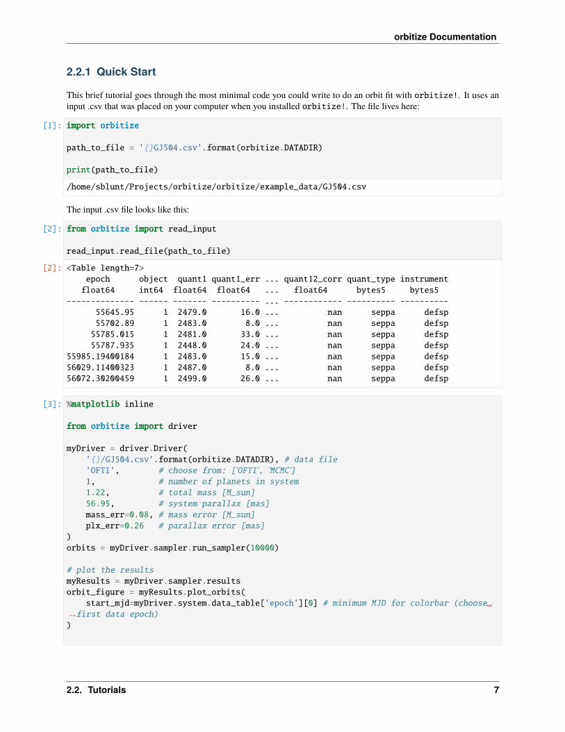
2.2.1 Quick Start
This brief tutorial goes through the most minimal code you could write to do an orbit fit with orbitize!. It uses aninput .csv that was placed on your computer when you installed orbitize!. The file lives here:
[1]: import orbitize
path_to_file = 'GJ504.csv'.format(orbitize.DATADIR)
print(path_to_file)
/home/sblunt/Projects/orbitize/orbitize/example_data/GJ504.csv
The input .csv file looks like this:
[2]: from orbitize import read_input
read_input.read_file(path_to_file)
[2]: <Table length=7>epoch object quant1 quant1_err ... quant12_corr quant_type instrumentfloat64 int64 float64 float64 ... float64 bytes5 bytes5
-------------- ------ ------- ---------- ... ------------ ---------- ----------55645.95 1 2479.0 16.0 ... nan seppa defsp55702.89 1 2483.0 8.0 ... nan seppa defsp55785.015 1 2481.0 33.0 ... nan seppa defsp55787.935 1 2448.0 24.0 ... nan seppa defsp
55985.19400184 1 2483.0 15.0 ... nan seppa defsp56029.11400323 1 2487.0 8.0 ... nan seppa defsp56072.30200459 1 2499.0 26.0 ... nan seppa defsp
[3]: %matplotlib inline
from orbitize import driver
myDriver = driver.Driver('/GJ504.csv'.format(orbitize.DATADIR), # data file'OFTI', # choose from: ['OFTI', 'MCMC']1, # number of planets in system1.22, # total mass [M_sun]56.95, # system parallax [mas]mass_err=0.08, # mass error [M_sun]plx_err=0.26 # parallax error [mas]
)orbits = myDriver.sampler.run_sampler(10000)
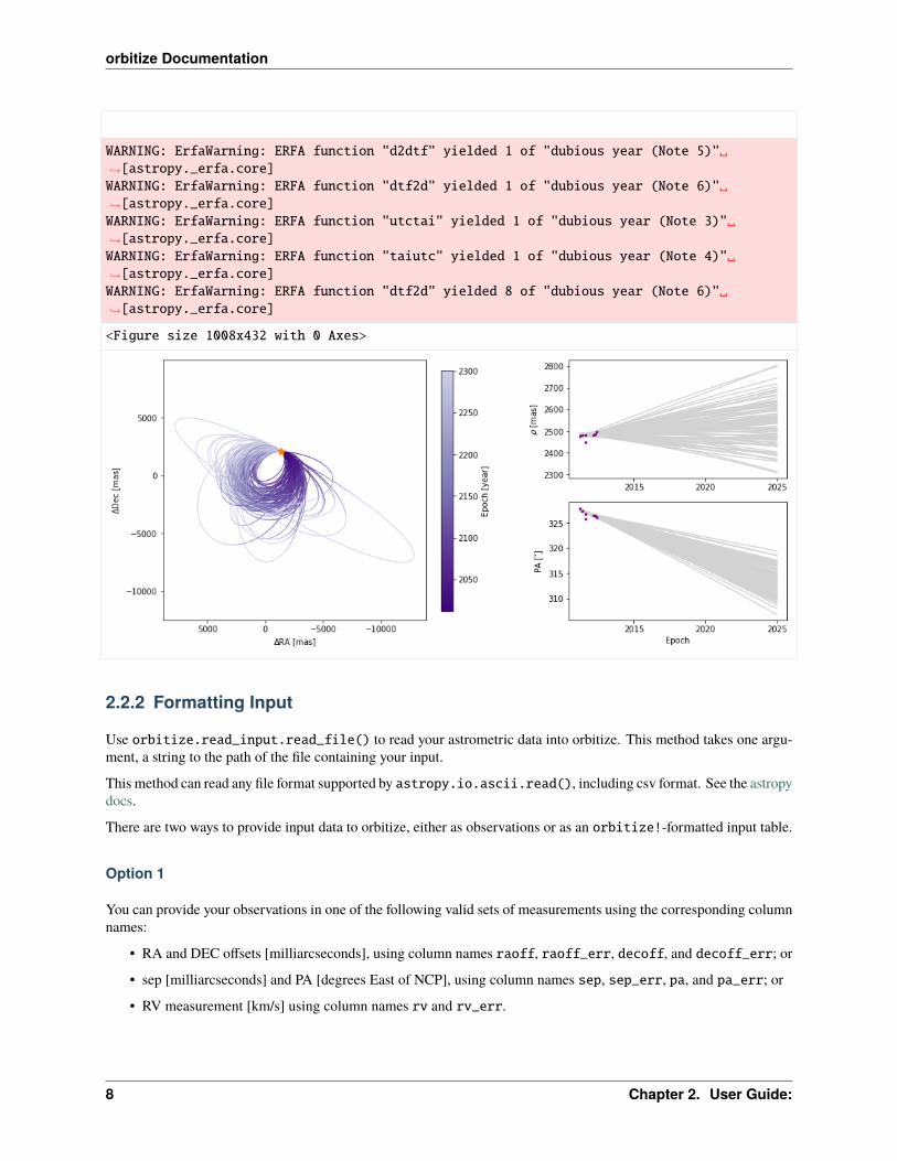
# plot the resultsmyResults = myDriver.sampler.resultsorbit_figure = myResults.plot_orbits(
start_mjd=myDriver.system.data_table['epoch'][0] # minimum MJD for colorbar (choose→˓first data epoch))
2.2. Tutorials 7
orbitize Documentation
WARNING: ErfaWarning: ERFA function "d2dtf" yielded 1 of "dubious year (Note 5)"→˓[astropy._erfa.core]WARNING: ErfaWarning: ERFA function "dtf2d" yielded 1 of "dubious year (Note 6)"→˓[astropy._erfa.core]WARNING: ErfaWarning: ERFA function "utctai" yielded 1 of "dubious year (Note 3)"→˓[astropy._erfa.core]WARNING: ErfaWarning: ERFA function "taiutc" yielded 1 of "dubious year (Note 4)"→˓[astropy._erfa.core]WARNING: ErfaWarning: ERFA function "dtf2d" yielded 8 of "dubious year (Note 6)"→˓[astropy._erfa.core]
<Figure size 1008x432 with 0 Axes>
2.2.2 Formatting Input
Use orbitize.read_input.read_file() to read your astrometric data into orbitize. This method takes one argu-ment, a string to the path of the file containing your input.
This method can read any file format supported by astropy.io.ascii.read(), including csv format. See the astropydocs.
There are two ways to provide input data to orbitize, either as observations or as an orbitize!-formatted input table.
Option 1
You can provide your observations in one of the following valid sets of measurements using the corresponding columnnames:
• RA and DEC offsets [milliarcseconds], using column names raoff, raoff_err, decoff, and decoff_err; or
• sep [milliarcseconds] and PA [degrees East of NCP], using column names sep, sep_err, pa, and pa_err; or
• RV measurement [km/s] using column names rv and rv_err.
8 Chapter 2. User Guide:
orbitize Documentation
Each row must also have a column for epoch and object. Epoch is the date of the observation, in MJD (JD-2400000.5).If this method thinks you have provided a date in JD, it will print a warning and attempt to convert to MJD. Objects arenumbered with integers, where the primary/central object is 0.
You may mix and match these three valid measurement formats in the same input file. So, you can have some epochswith RA/DEC offsets and others in separation/PA measurements.
If you have, for example, one RV measurement of a star and three astrometric measurements of an orbiting planet, youshould put 0 in the object column for the RV point, and 1 in the columns for the astrometric measurements.
This method will look for columns with the above labels in whatever file format you choose so if you encounter errors,be sure to double check the column labels in your input file.
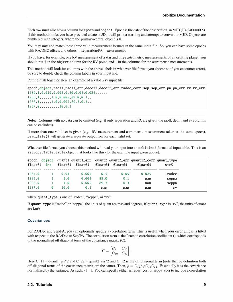
Putting it all together, here an example of a valid .csv input file:
epoch,object,raoff,raoff_err,decoff,decoff_err,radec_corr,sep,sep_err,pa,pa_err,rv,rv_err1234,1,0.010,0.005,0.50,0.05,0.025,,,,,,1235,1,,,,,,1.0,0.005,89.0,0.1,,1236,1,,,,,,1.0,0.005,89.3,0.3,,1237,0,,,,,,,,,,10,0.1
Note: Columns with no data can be omitted (e.g. if only separation and PA are given, the raoff, deoff, and rv columnscan be excluded).
If more than one valid set is given (e.g. RV measurement and astrometric measurement taken at the same epoch),read_file() will generate a separate output row for each valid set.
Whatever file format you choose, this method will read your input into an orbitize!-formatted input table. This is anastropy.Table.table object that looks like this (for the example input given above):
epoch object quant1 quant1_err quant2 quant2_err quant12_corr quant_typefloat64 int float64 float64 float64 float64 float64 str5------- ------ ------- ---------- ------- ---------- ------------ ----------1234.0 1 0.01 0.005 0.5 0.05 0.025 radec1235.0 1 1.0 0.005 89.0 0.1 nan seppa1236.0 1 1.0 0.005 89.3 0.3 nan seppa1237.0 0 10.0 0.1 nan nan nan rv
where quant_type is one of “radec”, “seppa”, or “rv”.
If quant_type is “radec” or “seppa”, the units of quant are mas and degrees, if quant_type is “rv”, the units of quantare km/s.
Covariances
For RA/Dec and Sep/PA, you can optionally specify a correlation term. This is useful when your error ellipse is tiltedwith respect to the RA/Dec or Sep/PA. The correlation term is the Pearson correlation coefficient (), which correspondsto the normalized off diagonal term of the covariance matrix (C):
𝐶 =
[𝐶11 𝐶12
𝐶12 𝐶22
].
Here C_11 = quant1_err^2 and C_22 = quant2_err^2 and C_12 is the off diagonal term (note that by definition bothoff-diagonal terms of the covariance matrix are the same). Then, 𝜌 = 𝐶12/
√𝐶11𝐶22. Essentially it is the covariance
normalized by the variance. As such, -1 1. You can specify either as radec_corr or seppa_corr to include a correlation
2.2. Tutorials 9
orbitize Documentation
in the errors. By definition, both are dimensionless, but one will correspond to RA/Dec and the other to Sep/PA. If nocorrelations are specified, it will assume the errors are uncorrelated ( = 0). In many papers, the errors are assumed tobe uncorrelated. An example of real world data that reports correlations is this GRAVITY paper where table 2 reportsthe correlation values and figure 4 shows how the error ellipses are tilted.
In the example above, we specify the first epoch has a positive correlation between the uncertainties in RA and Decusing the radec_corr column in the input data. This gets translated into the quant12_corr field in orbitize!-format. No correlations are specified for the other entries, and so we will assume those errors are uncorrelated. Afterthis is specified, handling of the correlations will be done automatically when computing model likelihoods. There’snothing else you have to do after this step!
Option 2
Alternatively, you can also supply a data file with the columns already corresponding to the orbitize!-formattedinput table (see above for column names). This may be useful if you are wanting to use the output of thewrite_orbitize_input method (e.g. using some input prepared by another orbitize! user).
Note: When providing data with columns in the orbitize format, there should be no empty cells. As in the examplebelow, when quant2 is not applicable, the cell should contain nan.
2.2.3 OFTI Introduction
by Isabel Angelo and Sarah Blunt (2018)
OFTI (Orbits For The Impatient) is an orbit-generating algorithm designed specifically to handle data covering shortfractions of long-period exoplanets (Blunt et al. 2017). Here we go through steps of using OFTI within orbitize!
[1]: import orbitize
Basic Orbit Generating
Orbits are generated in OFTI through a Driver class within orbitize. Once we have imported this class:
[2]: import orbitize.driver
we can initialize a Driver object specific to our data:
[3]: myDriver = orbitize.driver.Driver('/GJ504.csv'.format(orbitize.DATADIR), # path to→˓data file
'OFTI', # name of algorithm for orbit-fitting1, # number of secondary bodies in system1.22, # total mass [M_sun]56.95, # total parallax of system [mas]mass_err=0.08, # mass error [M_sun]plx_err=0.26) # parallax error [mas]
Because OFTI is an object class within orbitize, we can assign all of the OFTI attributes onto a variable (s). We can thengenerate orbits for s using a function called run_sampler, a method of the OFTI class. The run_sampler methodtakes in the desired number of accepted orbits as an input.
Here we use run OFTI to randomly generate orbits until 1000 are accepted:
10 Chapter 2. User Guide:
orbitize Documentation
[4]: s = myDriver.samplerorbits = s.run_sampler(1000)
We have now generated 1000 possible orbits for our system. Here, orbits is a (1000 x 8) array, where each of the1000 elements corresponds to a single orbit. An orbit is represented by 8 orbital elements.
Here is an example of what an accepted orbit looks like from orbitize:
[5]: orbits[0]
[5]: array([4.93916907e+01, 8.90197501e-03, 2.63925411e+00, 2.44962990e+00,9.31508665e-01, 1.20302112e-01, 5.74242058e+01, 1.22728974e+00])
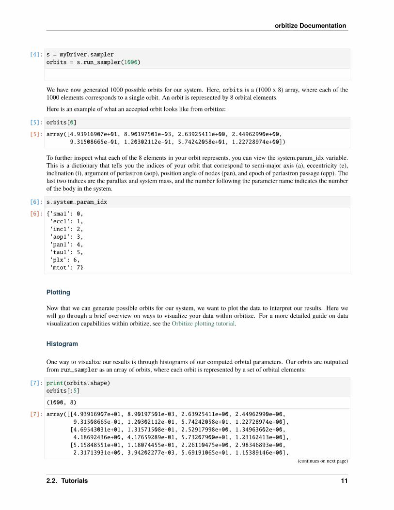
To further inspect what each of the 8 elements in your orbit represents, you can view the system.param_idx variable.This is a dictionary that tells you the indices of your orbit that correspond to semi-major axis (a), eccentricity (e),inclination (i), argument of periastron (aop), position angle of nodes (pan), and epoch of periastron passage (epp). Thelast two indices are the parallax and system mass, and the number following the parameter name indicates the numberof the body in the system.
[6]: s.system.param_idx
[6]: 'sma1': 0,'ecc1': 1,'inc1': 2,'aop1': 3,'pan1': 4,'tau1': 5,'plx': 6,'mtot': 7
Plotting
Now that we can generate possible orbits for our system, we want to plot the data to interpret our results. Here wewill go through a brief overview on ways to visualize your data within orbitize. For a more detailed guide on datavisualization capabilities within orbitize, see the Orbitize plotting tutorial.
Histogram
One way to visualize our results is through histograms of our computed orbital parameters. Our orbits are outputtedfrom run_sampler as an array of orbits, where each orbit is represented by a set of orbital elements:
[7]: print(orbits.shape)orbits[:5]
(1000, 8)
[7]: array([[4.93916907e+01, 8.90197501e-03, 2.63925411e+00, 2.44962990e+00,9.31508665e-01, 1.20302112e-01, 5.74242058e+01, 1.22728974e+00],[4.69543031e+01, 1.31571508e-01, 2.52917998e+00, 1.34963602e+00,4.18692436e+00, 4.17659289e-01, 5.73207900e+01, 1.23162413e+00],[5.15848551e+01, 1.18074455e-01, 2.26110475e+00, 2.98346893e+00,2.31713931e+00, 3.94202277e-03, 5.69191065e+01, 1.15389146e+00],
(continues on next page)
2.2. Tutorials 11
orbitize Documentation
(continued from previous page)
[3.89558225e+01, 3.71357464e-01, 2.94801131e+00, 3.08542398e+00,4.77645562e+00, 7.15043369e-01, 5.72827098e+01, 1.05721164e+00],[8.19463988e+01, 1.45955646e-02, 2.11512811e+00, 4.52064036e+00,4.44802306e+00, 9.32004660e-01, 5.72429430e+01, 1.35323242e+00]])
We can effectively view outputs from run_sampler by creating a histogram of a given orbit element to see its distri-bution of possible values. Our system.param_idx dictionary is useful here. We can use it to determine the index of agiven orbit that corresponds to the orbital element we are interested in:
[8]: s.system.param_idx
[8]: 'sma1': 0,'ecc1': 1,'inc1': 2,'aop1': 3,'pan1': 4,'tau1': 5,'plx': 6,'mtot': 7
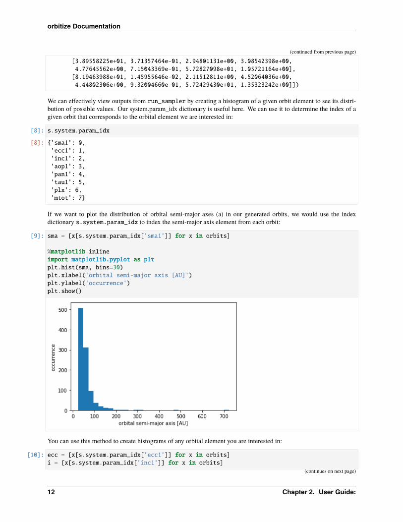
If we want to plot the distribution of orbital semi-major axes (a) in our generated orbits, we would use the indexdictionary s.system.param_idx to index the semi-major axis element from each orbit:
[9]: sma = [x[s.system.param_idx['sma1']] for x in orbits]
%matplotlib inlineimport matplotlib.pyplot as pltplt.hist(sma, bins=30)plt.xlabel('orbital semi-major axis [AU]')plt.ylabel('occurrence')plt.show()
You can use this method to create histograms of any orbital element you are interested in:
[10]: ecc = [x[s.system.param_idx['ecc1']] for x in orbits]i = [x[s.system.param_idx['inc1']] for x in orbits]
(continues on next page)
12 Chapter 2. User Guide:
orbitize Documentation
(continued from previous page)
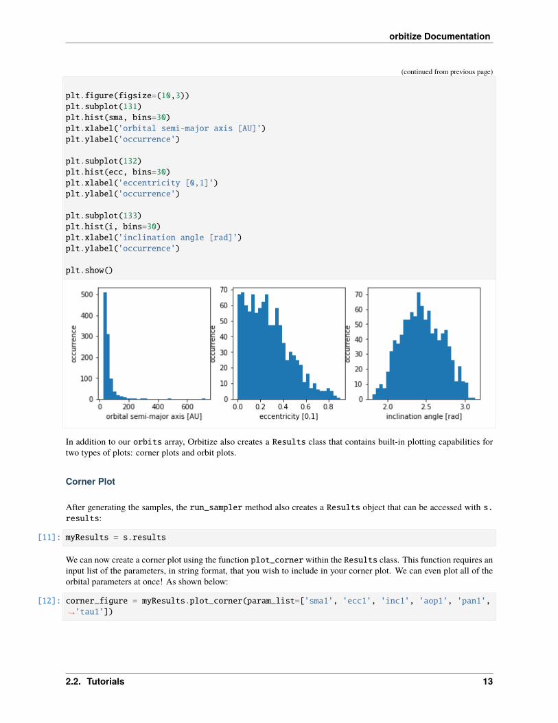
plt.figure(figsize=(10,3))plt.subplot(131)plt.hist(sma, bins=30)plt.xlabel('orbital semi-major axis [AU]')plt.ylabel('occurrence')
plt.subplot(132)plt.hist(ecc, bins=30)plt.xlabel('eccentricity [0,1]')plt.ylabel('occurrence')
plt.subplot(133)plt.hist(i, bins=30)plt.xlabel('inclination angle [rad]')plt.ylabel('occurrence')
plt.show()
In addition to our orbits array, Orbitize also creates a Results class that contains built-in plotting capabilities fortwo types of plots: corner plots and orbit plots.
Corner Plot
After generating the samples, the run_sampler method also creates a Results object that can be accessed with s.results:
[11]: myResults = s.results
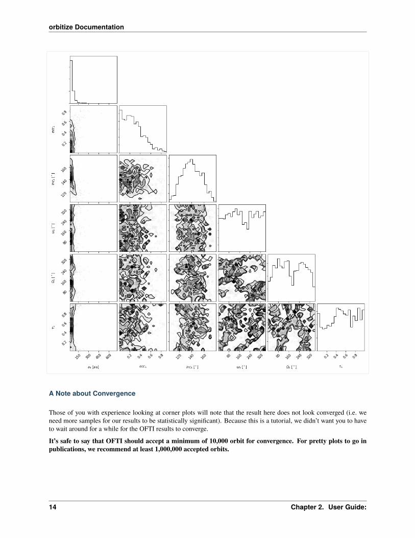
We can now create a corner plot using the function plot_corner within the Results class. This function requires aninput list of the parameters, in string format, that you wish to include in your corner plot. We can even plot all of theorbital parameters at once! As shown below:
[12]: corner_figure = myResults.plot_corner(param_list=['sma1', 'ecc1', 'inc1', 'aop1', 'pan1',→˓'tau1'])
2.2. Tutorials 13
orbitize Documentation
A Note about Convergence
Those of you with experience looking at corner plots will note that the result here does not look converged (i.e. weneed more samples for our results to be statistically significant). Because this is a tutorial, we didn’t want you to haveto wait around for a while for the OFTI results to converge.
It’s safe to say that OFTI should accept a minimum of 10,000 orbit for convergence. For pretty plots to go inpublications, we recommend at least 1,000,000 accepted orbits.
14 Chapter 2. User Guide:
orbitize Documentation
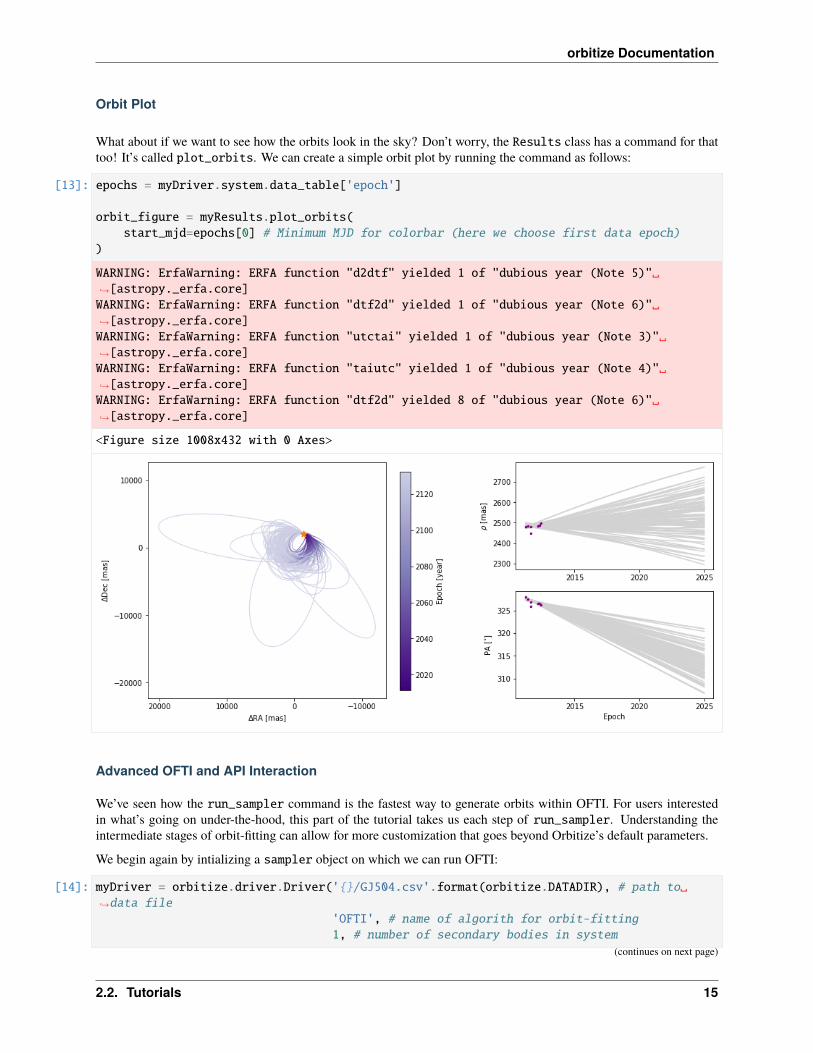
Orbit Plot
What about if we want to see how the orbits look in the sky? Don’t worry, the Results class has a command for thattoo! It’s called plot_orbits. We can create a simple orbit plot by running the command as follows:
[13]: epochs = myDriver.system.data_table['epoch']
orbit_figure = myResults.plot_orbits(start_mjd=epochs[0] # Minimum MJD for colorbar (here we choose first data epoch)
)
WARNING: ErfaWarning: ERFA function "d2dtf" yielded 1 of "dubious year (Note 5)"→˓[astropy._erfa.core]WARNING: ErfaWarning: ERFA function "dtf2d" yielded 1 of "dubious year (Note 6)"→˓[astropy._erfa.core]WARNING: ErfaWarning: ERFA function "utctai" yielded 1 of "dubious year (Note 3)"→˓[astropy._erfa.core]WARNING: ErfaWarning: ERFA function "taiutc" yielded 1 of "dubious year (Note 4)"→˓[astropy._erfa.core]WARNING: ErfaWarning: ERFA function "dtf2d" yielded 8 of "dubious year (Note 6)"→˓[astropy._erfa.core]
<Figure size 1008x432 with 0 Axes>
Advanced OFTI and API Interaction
We’ve seen how the run_sampler command is the fastest way to generate orbits within OFTI. For users interestedin what’s going on under-the-hood, this part of the tutorial takes us each step of run_sampler. Understanding theintermediate stages of orbit-fitting can allow for more customization that goes beyond Orbitize’s default parameters.
We begin again by intializing a sampler object on which we can run OFTI:
[14]: myDriver = orbitize.driver.Driver('/GJ504.csv'.format(orbitize.DATADIR), # path to→˓data file
'OFTI', # name of algorith for orbit-fitting1, # number of secondary bodies in system
(continues on next page)
2.2. Tutorials 15
orbitize Documentation
(continued from previous page)
1.22, # total mass [M_sun]56.95, # total parallax of system [mas]mass_err=0.08, # mass error [M_sun]plx_err=0.26) # parallax error [mas]
[15]: s = myDriver.sampler
In orbitize, the first thing that OFTI does is prepare an initial set of possible orbits for our object through a functioncalled prepare_samples, which takes in the number of orbits to generate as an input. For example, we can generate100,000 orbits as follows:
[16]: samples = s.prepare_samples(100000)
Here, samples is an array of randomly generated orbits that have been scaled-and-rotated to fit our astrometric ob-servations. The first and second dimension of this array are the number of orbital elements and total orbits generated,respectively. In other words, each element in samples represents the value of a particular orbital element for eachgenerated orbit:
[17]: print('samples: ', samples.shape)print('first element of samples: ', samples[0].shape)
samples: (8, 100000)first element of samples: (100000,)
Once our initial set of orbits is generated, the orbits are vetted for likelihood in a function called reject. This functioncomputes the probability of an orbit based on its associated chi squared. It then rejects orbits with lower likelihoodsand accepts the orbits that are more probable. The output of this function is an array of possible orbits for our inputsystem.
[18]: orbits, lnlikes = s.reject(samples)
Our orbits array represents the final orbits that are output by OFTI. Each element in this array contains the 8 orbitalelements that are computed by orbitize:
[19]: orbits.shape
[19]: (1, 8)
We can synthesize this sequence with the run_sampler() command, which runs through the steps above until the inputnumber of orbits has been accepted. Additionally, we can specify the number of orbits generated by prepare_sampleseach time the sequence is initiated with an argument called num_samples. Higher values for num_sampleswill outputmore accepted orbits, but may take longer to run since all initially prepared orbits will be run through the rejection step.
[20]: orbits = s.run_sampler(100, num_samples=1000)
16 Chapter 2. User Guide:
orbitize Documentation
Saving and Loading Results
Finally, we can save our generated orbits in a file that can be easily read for future use and analysis. Here we willwalk through the steps of saving a set of orbits to a file in hdf5 format. The easiest way to do this is using orbitize.Results.save_results():
[21]: s.results.save_results('orbits.hdf5')
Now when you are ready to use your orbits data, it is easily accessible through the file we’ve created. One way to dothis is to load the data into a new results object; in this way you can make use of the functions that we learn before,like plot_corner and plot_orbits. To do this, use the results module:
[22]: import orbitize.resultsloaded_results = orbitize.results.Results() # create a blank results object to load the→˓dataloaded_results.load_results('orbits.hdf5')
Alternatively, you can directly access the saved data using the h5py module:
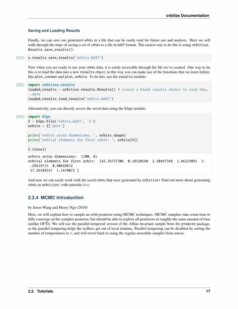
[23]: import h5pyf = h5py.File('orbits.hdf5', 'r')orbits = f['post']
print('orbits array dimensions: ', orbits.shape)print('orbital elements for first orbit: ', orbits[0])
f.close()
orbits array dimensions: (100, 8)orbital elements for first orbit: [42.56737306 0.18520168 2.50497349 1.46225095 3.→˓29419715 0.6064961257.26589357 1.1478072 ]
And now we can easily work with the saved orbits that were generated by orbitize! Find out more about generatingorbits in orbitize! with tutorials here.
2.2.4 MCMC Introduction
by Jason Wang and Henry Ngo (2018)
Here, we will explain how to sample an orbit posterior using MCMC techniques. MCMC samplers take some time tofully converge on the complex posterior, but should be able to explore all posteriors in roughly the same amount of time(unlike OFTI). We will use the parallel-tempered version of the Affine-invariant sample from the ptemcee package,as the parallel tempering helps the walkers get out of local minima. Parallel-tempering can be disabled by setting thenumber of temperatures to 1, and will revert back to using the regular ensemble sampler from emcee.
2.2. Tutorials 17

orbitize Documentation
Read in Data and Set up Sampler
We use orbitize.driver.Driver to streamline the processes of reading in data, setting up the two-body interaction,and setting up the MCMC sampler.
When setting up the sampler, we need to decide how many temperatures and how many walkers per temperature to use.Increasing the number of temperatures further ensures your walkers will explore all of parameter space and will not getstuck in local minima. Increasing the number of walkers gives you more samples to use, and, for the Affine-invariantsampler, a minimum number is required for good convergence. Of course, the tradeoff is that more samplers meansmore computation time. We find 20 temperatures and 1000 walkers to be reliable for convergence. Since this is atutorial meant to be run quickly, we use fewer walkers and temperatures here.
Note that we will only use the samples from the lowest-temperature walkers. We also assume that our astrometricmeasurements follow a Gaussian distribution.
orbitize can also fit for the total mass of the system and system parallax, including marginalizing over the uncertain-ties in those parameters.
[1]: import numpy as np
import orbitizefrom orbitize import driverimport multiprocessing as mp
filename = "/GJ504.csv".format(orbitize.DATADIR)
# system parametersnum_secondary_bodies = 1total_mass = 1.75 # [Msol]plx = 51.44 # [mas]mass_err = 0.05 # [Msol]plx_err = 0.12 # [mas]
# MCMC parametersnum_temps = 5num_walkers = 20num_threads = 2 # or a different number if you prefer, mp.cpu_count() for example
my_driver = driver.Driver(filename, 'MCMC', num_secondary_bodies, total_mass, plx, mass_err=mass_err, plx_
→˓err=plx_err,mcmc_kwargs='num_temps': num_temps, 'num_walkers': num_walkers, 'num_threads': num_
→˓threads)
18 Chapter 2. User Guide:
orbitize Documentation
Running the MCMC Sampler
We need to pick how many steps the MCMC sampler should sample. Additionally, because the samples are correlated,we often only save every nth sample. This helps when we run a lot of samples, because saving all the samples requirestoo much disk space and many samples are unnecessary because they are correlated.
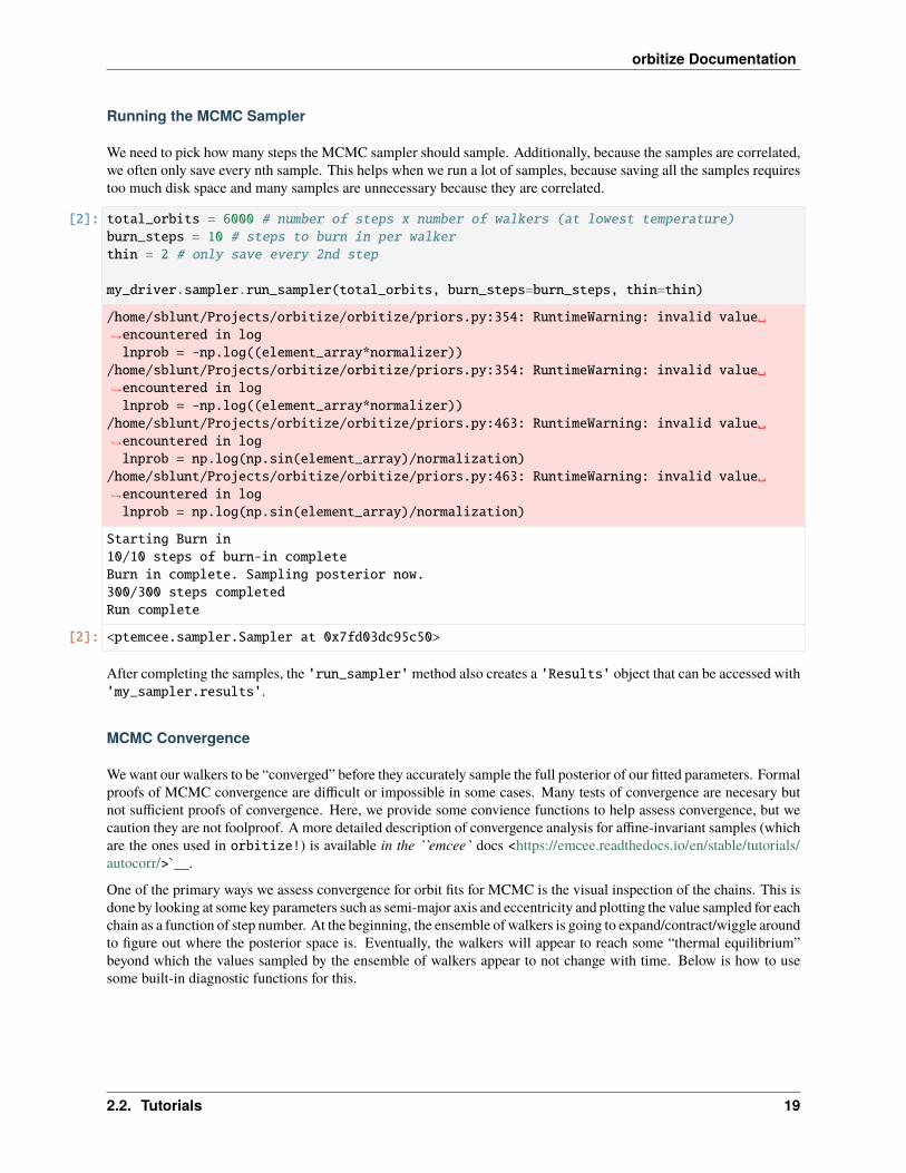
[2]: total_orbits = 6000 # number of steps x number of walkers (at lowest temperature)burn_steps = 10 # steps to burn in per walkerthin = 2 # only save every 2nd step
my_driver.sampler.run_sampler(total_orbits, burn_steps=burn_steps, thin=thin)
/home/sblunt/Projects/orbitize/orbitize/priors.py:354: RuntimeWarning: invalid value→˓encountered in loglnprob = -np.log((element_array*normalizer))
/home/sblunt/Projects/orbitize/orbitize/priors.py:354: RuntimeWarning: invalid value→˓encountered in loglnprob = -np.log((element_array*normalizer))
/home/sblunt/Projects/orbitize/orbitize/priors.py:463: RuntimeWarning: invalid value→˓encountered in loglnprob = np.log(np.sin(element_array)/normalization)
/home/sblunt/Projects/orbitize/orbitize/priors.py:463: RuntimeWarning: invalid value→˓encountered in loglnprob = np.log(np.sin(element_array)/normalization)
Starting Burn in10/10 steps of burn-in completeBurn in complete. Sampling posterior now.300/300 steps completedRun complete
[2]: <ptemcee.sampler.Sampler at 0x7fd03dc95c50>
After completing the samples, the 'run_sampler'method also creates a 'Results' object that can be accessed with'my_sampler.results'.
MCMC Convergence
We want our walkers to be “converged” before they accurately sample the full posterior of our fitted parameters. Formalproofs of MCMC convergence are difficult or impossible in some cases. Many tests of convergence are necesary butnot sufficient proofs of convergence. Here, we provide some convience functions to help assess convergence, but wecaution they are not foolproof. A more detailed description of convergence analysis for affine-invariant samples (whichare the ones used in orbitize!) is available in the ``emcee` docs <https://emcee.readthedocs.io/en/stable/tutorials/autocorr/>`__.
One of the primary ways we assess convergence for orbit fits for MCMC is the visual inspection of the chains. This isdone by looking at some key parameters such as semi-major axis and eccentricity and plotting the value sampled for eachchain as a function of step number. At the beginning, the ensemble of walkers is going to expand/contract/wiggle aroundto figure out where the posterior space is. Eventually, the walkers will appear to reach some “thermal equilibrium”beyond which the values sampled by the ensemble of walkers appear to not change with time. Below is how to usesome built-in diagnostic functions for this.
2.2. Tutorials 19

orbitize Documentation
Diagnostic Functions
The Sampler object also has two convenience functions to examine and modify the walkers in order to diagnose MCMCperformance. Note that in this example we have not run things for long enough with enough walkers to actually seeconvergence, so this is merely a demo of the API.
First, we can examine 5 randomly selected walkers for two parameters: semimajor axis and eccentricity. We expect150 steps per walker since there were 6,000 orbits requested with 20 walkers, so that’s 300 orbits per walker. However,we have thinned by a factor of 2, so there are 150 saved steps.
[3]: sma_chains, ecc_chains = my_driver.sampler.examine_chains(param_list=['sma1','ecc1'], n_→˓walkers=5)
This method returns one matplotlib Figure object for each parameter. If no param_list given, all parameters arereturned. Here, we told it to plot 5 randomly selected walkers but we could have specified exactly which walkers withthe walker_list keyword. The step_range keyword also determines which steps in the chain are plotted (whennothing is given, the default is to plot all steps). We can also have these plots automatically generate if we calledrun_sampler with examine_chains=True.
Note that this is just a convenience function. It is possible to recreate these chains from reshaping the posterior samplesand selecting the correct entries.
20 Chapter 2. User Guide:
orbitize Documentation
The second diagnostic tool is the chop_chains, which allows us to remove entries from the beginning and/or endof a chain. This updates the corresponding Results object stored in sampler (in this case, my_driver.sampler.results). The burn parameter specifies the number of steps to remove from the beginning (i.e. to add a burn-in to yourchain) and the trim parameter specifies the number of steps to remove from the end. If only one parameter is given,it is assumed to be a burn value. If trim is not zero, the sampler object is also updated so that the current position(sampler.curr_pos) matches the new end point. This allows us to continue MCMC runs at the correct position, evenif we have removed the last few steps of the chain.
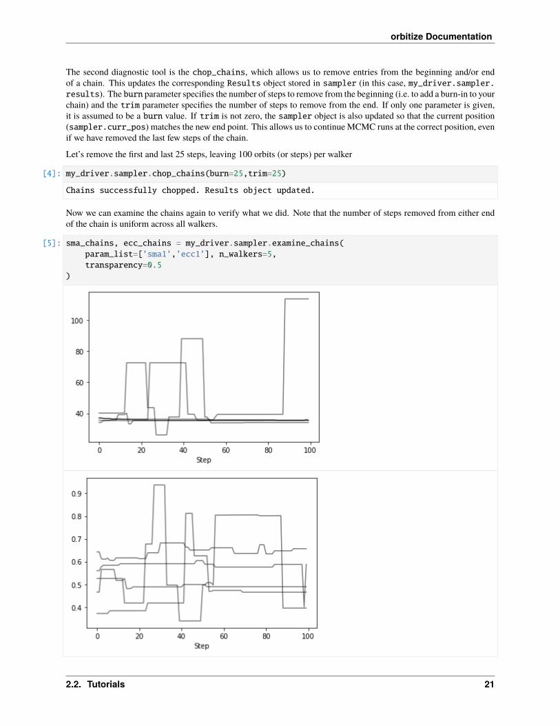
Let’s remove the first and last 25 steps, leaving 100 orbits (or steps) per walker
[4]: my_driver.sampler.chop_chains(burn=25,trim=25)
Chains successfully chopped. Results object updated.
Now we can examine the chains again to verify what we did. Note that the number of steps removed from either endof the chain is uniform across all walkers.
[5]: sma_chains, ecc_chains = my_driver.sampler.examine_chains(param_list=['sma1','ecc1'], n_walkers=5,transparency=0.5
)
2.2. Tutorials 21
orbitize Documentation
Plotting Basics
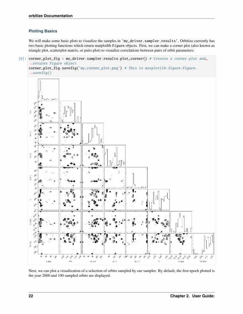
We will make some basic plots to visualize the samples in 'my_driver.sampler.results'. Orbitize currently hastwo basic plotting functions which return matplotlib Figure objects. First, we can make a corner plot (also known astriangle plot, scatterplot matrix, or pairs plot) to visualize correlations between pairs of orbit parameters:
[6]: corner_plot_fig = my_driver.sampler.results.plot_corner() # Creates a corner plot and→˓returns Figure objectcorner_plot_fig.savefig('my_corner_plot.png') # This is matplotlib.figure.Figure.→˓savefig()
Next, we can plot a visualization of a selection of orbits sampled by our sampler. By default, the first epoch plotted isthe year 2000 and 100 sampled orbits are displayed.
22 Chapter 2. User Guide:
orbitize Documentation
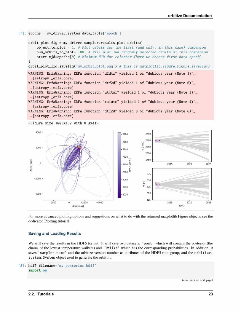
[7]: epochs = my_driver.system.data_table['epoch']
orbit_plot_fig = my_driver.sampler.results.plot_orbits(object_to_plot = 1, # Plot orbits for the first (and only, in this case) companionnum_orbits_to_plot= 100, # Will plot 100 randomly selected orbits of this companionstart_mjd=epochs[0] # Minimum MJD for colorbar (here we choose first data epoch)
)orbit_plot_fig.savefig('my_orbit_plot.png') # This is matplotlib.figure.Figure.savefig()
WARNING: ErfaWarning: ERFA function "d2dtf" yielded 1 of "dubious year (Note 5)"→˓[astropy._erfa.core]WARNING: ErfaWarning: ERFA function "dtf2d" yielded 1 of "dubious year (Note 6)"→˓[astropy._erfa.core]WARNING: ErfaWarning: ERFA function "utctai" yielded 1 of "dubious year (Note 3)"→˓[astropy._erfa.core]WARNING: ErfaWarning: ERFA function "taiutc" yielded 1 of "dubious year (Note 4)"→˓[astropy._erfa.core]WARNING: ErfaWarning: ERFA function "dtf2d" yielded 8 of "dubious year (Note 6)"→˓[astropy._erfa.core]
<Figure size 1008x432 with 0 Axes>
For more advanced plotting options and suggestions on what to do with the returned matplotlib Figure objects, see thededicated Plotting tutorial.
Saving and Loading Results
We will save the results in the HDF5 format. It will save two datasets: 'post' which will contain the posterior (thechains of the lowest temperature walkers) and 'lnlike' which has the corresponding probabilities. In addition, itsaves 'sampler_name' and the orbitize version number as attributes of the HDF5 root group, and the orbitize.system.System object used to generate the orbit fit.
[8]: hdf5_filename='my_posterior.hdf5'import os
(continues on next page)
2.2. Tutorials 23
orbitize Documentation
(continued from previous page)
# To avoid weird behaviours, delete saved file if it already exists from a previous run→˓of this notebookif os.path.isfile(hdf5_filename):
os.remove(hdf5_filename)my_driver.sampler.results.save_results(hdf5_filename)
Saving sampler results is a good idea when we want to analyze the results in a different script or when we want to savethe output of a long MCMC run to avoid having to re-run it in the future. We can then load the saved results into a newblank results object.
[9]: from orbitize import resultsloaded_results = results.Results() # Create blank results object for loadingloaded_results.load_results(hdf5_filename)
Instead of loading results into an orbitize.results.Results object, we can also directly access the saved data using the'h5py' python module.
[10]: import h5pyfilename = 'my_posterior.hdf5'hf = h5py.File(filename,'r') # Opens file for reading# Load up each dataset from hdf5 filesampler_name = np.str(hf.attrs['sampler_name'])post = np.array(hf.get('post'))lnlike = np.array(hf.get('lnlike'))hf.close() # Don't forget to close the file
2.2.5 Modifying Priors
by Sarah Blunt (2018)
Most often, you will use the Driver class to interact with orbitize. This class automatically reads your input file,creates all of the orbitize objects you need to run an orbit fit, and allows you to run the orbit fit. See the introductoryOFTI and MCMC tutorials for examples of working with this class.
However, sometimes you will want to work with the underlying methods directly. Doing this gives you control over thefunctionality Driver executes automatically, and allows you more flexibility.
Modifying priors is an example of something you might want to use the underlying API for. This tutorial walks youthrough how to do that.
Goals of this tutorial: - Learn to modify priors in orbitize - Learn how to fix a parameter at a specific value - Learnabout the structure of the orbitize code base
[1]: import numpy as npfrom matplotlib import pyplot as pltimport orbitizefrom orbitize import read_input, system, priors, sampler
24 Chapter 2. User Guide:
orbitize Documentation
Read in Data
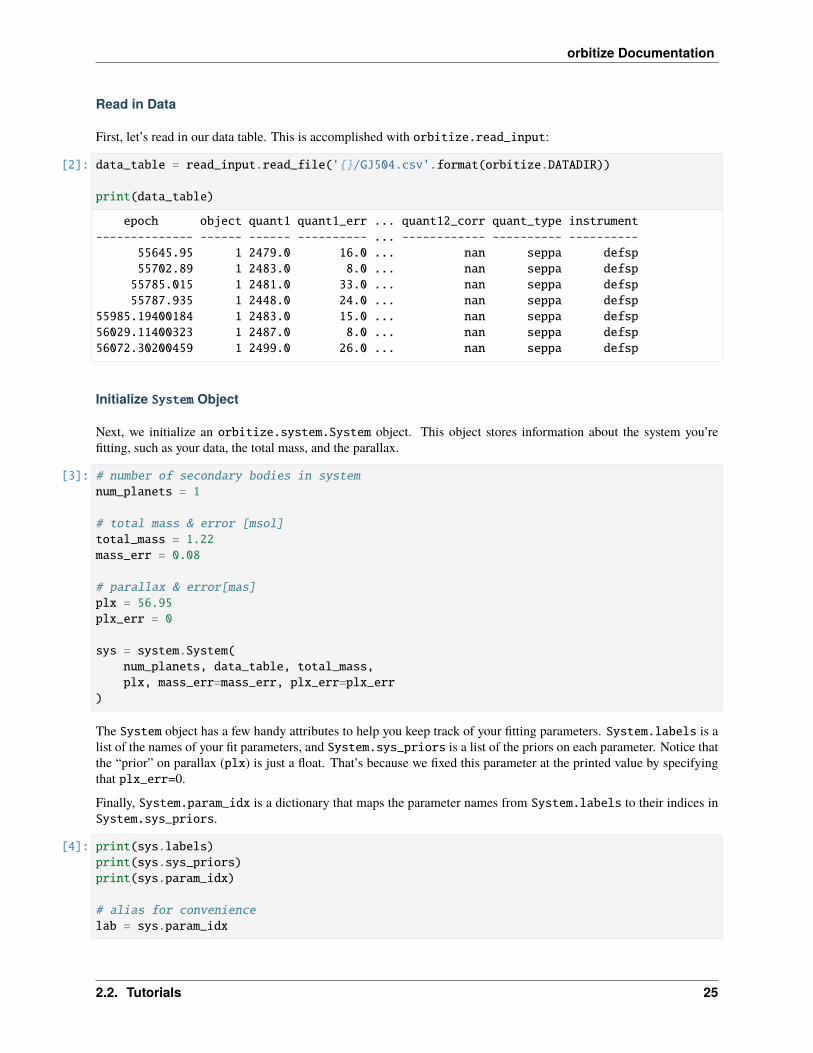
First, let’s read in our data table. This is accomplished with orbitize.read_input:
[2]: data_table = read_input.read_file('/GJ504.csv'.format(orbitize.DATADIR))
print(data_table)
epoch object quant1 quant1_err ... quant12_corr quant_type instrument-------------- ------ ------ ---------- ... ------------ ---------- ----------
55645.95 1 2479.0 16.0 ... nan seppa defsp55702.89 1 2483.0 8.0 ... nan seppa defsp55785.015 1 2481.0 33.0 ... nan seppa defsp55787.935 1 2448.0 24.0 ... nan seppa defsp
55985.19400184 1 2483.0 15.0 ... nan seppa defsp56029.11400323 1 2487.0 8.0 ... nan seppa defsp56072.30200459 1 2499.0 26.0 ... nan seppa defsp
Initialize System Object
Next, we initialize an orbitize.system.System object. This object stores information about the system you’refitting, such as your data, the total mass, and the parallax.
[3]: # number of secondary bodies in systemnum_planets = 1
# total mass & error [msol]total_mass = 1.22mass_err = 0.08
# parallax & error[mas]plx = 56.95plx_err = 0
sys = system.System(num_planets, data_table, total_mass,plx, mass_err=mass_err, plx_err=plx_err
)
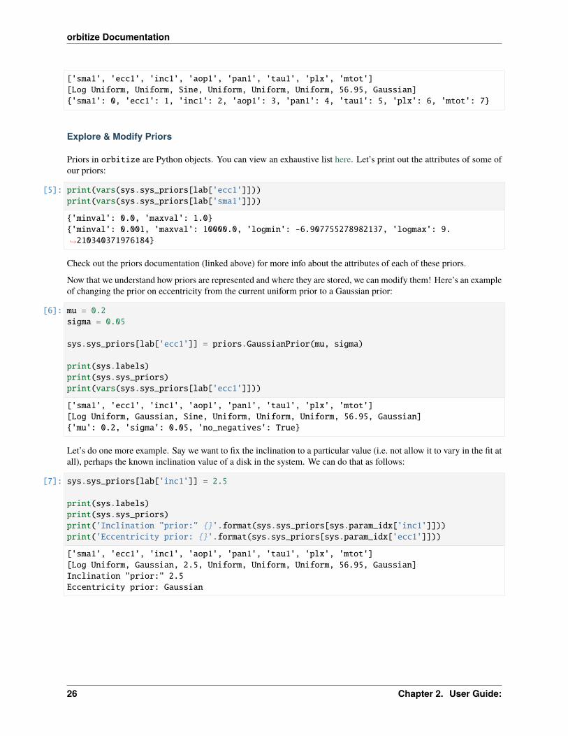
The System object has a few handy attributes to help you keep track of your fitting parameters. System.labels is alist of the names of your fit parameters, and System.sys_priors is a list of the priors on each parameter. Notice thatthe “prior” on parallax (plx) is just a float. That’s because we fixed this parameter at the printed value by specifyingthat plx_err=0.
Finally, System.param_idx is a dictionary that maps the parameter names from System.labels to their indices inSystem.sys_priors.
[4]: print(sys.labels)print(sys.sys_priors)print(sys.param_idx)
# alias for conveniencelab = sys.param_idx
2.2. Tutorials 25
orbitize Documentation
['sma1', 'ecc1', 'inc1', 'aop1', 'pan1', 'tau1', 'plx', 'mtot'][Log Uniform, Uniform, Sine, Uniform, Uniform, Uniform, 56.95, Gaussian]'sma1': 0, 'ecc1': 1, 'inc1': 2, 'aop1': 3, 'pan1': 4, 'tau1': 5, 'plx': 6, 'mtot': 7
Explore & Modify Priors
Priors in orbitize are Python objects. You can view an exhaustive list here. Let’s print out the attributes of some ofour priors:
[5]: print(vars(sys.sys_priors[lab['ecc1']]))print(vars(sys.sys_priors[lab['sma1']]))
'minval': 0.0, 'maxval': 1.0'minval': 0.001, 'maxval': 10000.0, 'logmin': -6.907755278982137, 'logmax': 9.→˓210340371976184
Check out the priors documentation (linked above) for more info about the attributes of each of these priors.
Now that we understand how priors are represented and where they are stored, we can modify them! Here’s an exampleof changing the prior on eccentricity from the current uniform prior to a Gaussian prior:
[6]: mu = 0.2sigma = 0.05
sys.sys_priors[lab['ecc1']] = priors.GaussianPrior(mu, sigma)
print(sys.labels)print(sys.sys_priors)print(vars(sys.sys_priors[lab['ecc1']]))
['sma1', 'ecc1', 'inc1', 'aop1', 'pan1', 'tau1', 'plx', 'mtot'][Log Uniform, Gaussian, Sine, Uniform, Uniform, Uniform, 56.95, Gaussian]'mu': 0.2, 'sigma': 0.05, 'no_negatives': True
Let’s do one more example. Say we want to fix the inclination to a particular value (i.e. not allow it to vary in the fit atall), perhaps the known inclination value of a disk in the system. We can do that as follows:
[7]: sys.sys_priors[lab['inc1']] = 2.5
print(sys.labels)print(sys.sys_priors)print('Inclination "prior:" '.format(sys.sys_priors[sys.param_idx['inc1']]))print('Eccentricity prior: '.format(sys.sys_priors[sys.param_idx['ecc1']]))
['sma1', 'ecc1', 'inc1', 'aop1', 'pan1', 'tau1', 'plx', 'mtot'][Log Uniform, Gaussian, 2.5, Uniform, Uniform, Uniform, 56.95, Gaussian]Inclination "prior:" 2.5Eccentricity prior: Gaussian
26 Chapter 2. User Guide:
orbitize Documentation
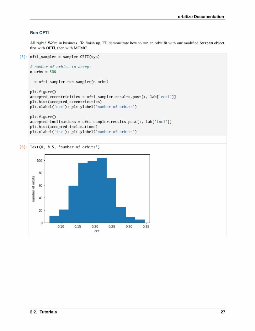
Run OFTI
All right! We’re in business. To finish up, I’ll demonstrate how to run an orbit fit with our modified System object,first with OFTI, then with MCMC.
[8]: ofti_sampler = sampler.OFTI(sys)
# number of orbits to acceptn_orbs = 500
_ = ofti_sampler.run_sampler(n_orbs)
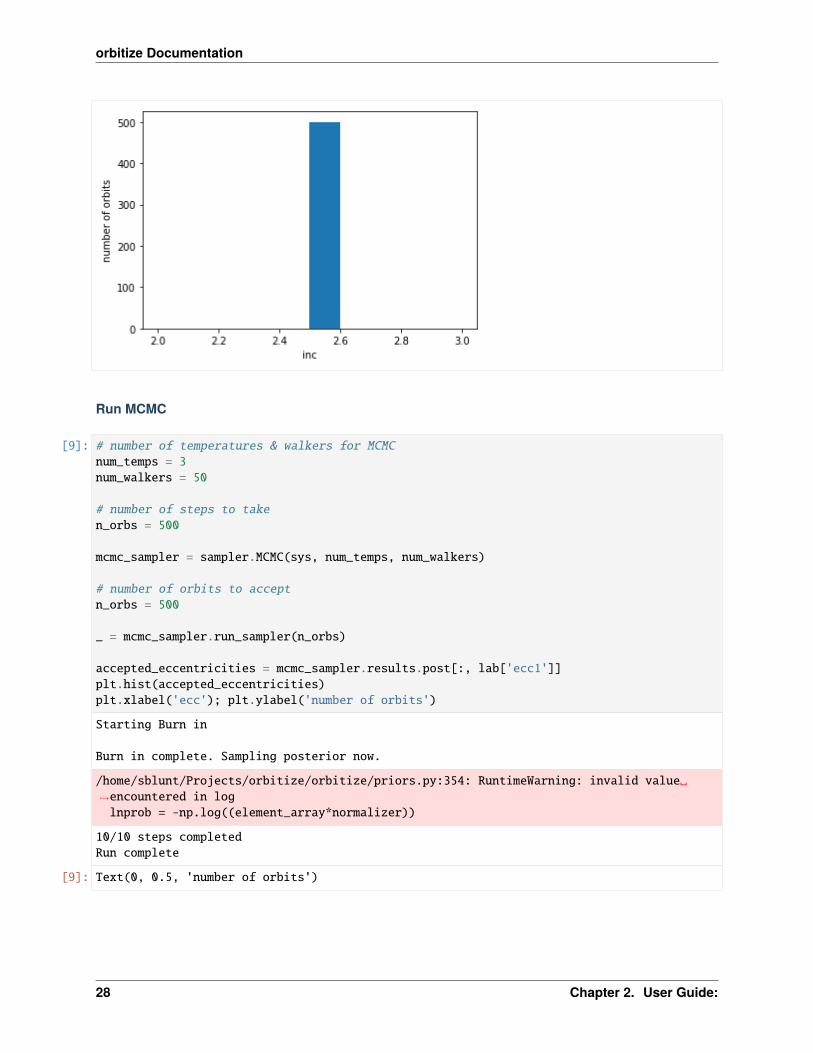
plt.figure()accepted_eccentricities = ofti_sampler.results.post[:, lab['ecc1']]plt.hist(accepted_eccentricities)plt.xlabel('ecc'); plt.ylabel('number of orbits')
plt.figure()accepted_inclinations = ofti_sampler.results.post[:, lab['inc1']]plt.hist(accepted_inclinations)plt.xlabel('inc'); plt.ylabel('number of orbits')
[8]: Text(0, 0.5, 'number of orbits')
2.2. Tutorials 27
orbitize Documentation
Run MCMC
[9]: # number of temperatures & walkers for MCMCnum_temps = 3num_walkers = 50
# number of steps to taken_orbs = 500
mcmc_sampler = sampler.MCMC(sys, num_temps, num_walkers)
# number of orbits to acceptn_orbs = 500
_ = mcmc_sampler.run_sampler(n_orbs)
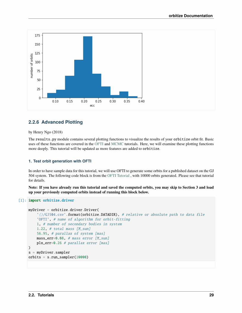
accepted_eccentricities = mcmc_sampler.results.post[:, lab['ecc1']]plt.hist(accepted_eccentricities)plt.xlabel('ecc'); plt.ylabel('number of orbits')
Starting Burn in
Burn in complete. Sampling posterior now.
/home/sblunt/Projects/orbitize/orbitize/priors.py:354: RuntimeWarning: invalid value→˓encountered in loglnprob = -np.log((element_array*normalizer))
10/10 steps completedRun complete
[9]: Text(0, 0.5, 'number of orbits')
28 Chapter 2. User Guide:
orbitize Documentation
2.2.6 Advanced Plotting
by Henry Ngo (2018)
The results.py module contains several plotting functions to visualize the results of your orbitize orbit fit. Basicuses of these functions are covered in the OFTI and MCMC tutorials. Here, we will examine these plotting functionsmore deeply. This tutorial will be updated as more features are added to orbitize.
1. Test orbit generation with OFTI
In order to have sample data for this tutorial, we will use OFTI to generate some orbits for a published dataset on the GJ504 system. The following code block is from the OFTI Tutorial , with 10000 orbits generated. Please see that tutorialfor details.
Note: If you have already run this tutorial and saved the computed orbits, you may skip to Section 3 and loadup your previously computed orbits instead of running this block below.
[1]: import orbitize.driver
myDriver = orbitize.driver.Driver('/GJ504.csv'.format(orbitize.DATADIR), # relative or absolute path to data file'OFTI', # name of algorithm for orbit-fitting1, # number of secondary bodies in system1.22, # total mass [M_sun]56.95, # parallax of system [mas]mass_err=0.08, # mass error [M_sun]plx_err=0.26 # parallax error [mas]
)s = myDriver.samplerorbits = s.run_sampler(10000)
2.2. Tutorials 29

orbitize Documentation
2. Accessing a Results object with computed orbits
After computing your orbits from either OFTI or MCMC, they are accessible as a Results object for further analysisand plotting. This object is an attribute of s, the sampler object defined above.
[2]: myResults = s.results # array of MxN array of orbital parameters (M orbits with N→˓parameters per orbit)
It is also useful to save this Results object to a file if we want to load up the same data later without re-computing theorbits.
[3]: myResults.save_results('plotting_tutorial_GJ504_results.hdf5')
For more information on the Results object, see below.
[4]: myResults?
Type: ResultsString form: <orbitize.results.Results object at 0x7fc0deecc6d0>File: ~/Projects/orbitize/orbitize/results.pyDocstring:A class to store accepted orbital configurations from the sampler
Args:system (orbitize.system.System): System object used to do the fit.sampler_name (string): name of sampler class that generated these results
(default: None).post (np.array of float): MxN array of orbital parameters
(posterior output from orbit-fitting process), where M is thenumber of orbits generated, and N is the number of varying orbitalparameters in the fit (default: None).
lnlike (np.array of float): M array of log-likelihoods corresponding tothe orbits described in ``post`` (default: None).
version_number (str): version of orbitize that produced these results.data (astropy.table.Table): output from ``orbitize.read_input.read_file()``curr_pos (np.array of float): for MCMC only. A multi-D array of the
current walker positions that is used for restarting a MCMC sampler.
Written: Henry Ngo, Sarah Blunt, 2018
API Update: Sarah Blunt, 2021
Note that you can also add more computed orbits to a results object with myResults.add_samples():
[5]: myResults.add_samples?
Signature: myResults.add_samples(orbital_params, lnlikes, curr_pos=None)Docstring:Add accepted orbits, their likelihoods, and the orbitize version numberto the results
Args:orbital_params (np.array): add sets of orbital params (could be multiple)
to resultslnlike (np.array): add corresponding lnlike values to results
(continues on next page)
30 Chapter 2. User Guide:
orbitize Documentation
(continued from previous page)
curr_pos (np.array of float): for MCMC only. A multi-D array of thecurrent walker positions
Written: Henry Ngo, 2018
API Update: Sarah Blunt, 2021File: ~/Projects/orbitize/orbitize/results.pyType: method
3. (Optional) Load up saved results object
If you are skipping the generation of all orbits because you would rather load from a file that saved the Results objectgenerated above, then execute this block to load it up. Otherwise, skip this block (however, nothing bad will happen ifyou run it even if you generated orbits above).
[6]: import orbitize.resultsif 'myResults' in locals():
del myResults # delete existing Results objectmyResults = orbitize.results.Results() # create empty Results objectmyResults.load_results('plotting_tutorial_GJ504_results.hdf5') # load from file
4. Using our Results object to make plots
In this tutorial, we’ll work with two plotting functions: plot_corner() makes a corner plot and plot_orbits()displays some or all of the computed orbits. Both plotting functions return matplotlib.pyplot.figure objects, which canbe displayed, further manipulated with matplotlib.pyplot functions, and saved.
[7]: %matplotlib inlineimport matplotlib.pyplot as plt
4.1 Corner plots
This function is a wrapper for corner.py and creates a display of the 2-D covariances between each pair of parametersas well as histograms for each parameter. These plots are known as “corner plots”, “pairs plots”, and “scatterplotmatrices”, as well as other names.
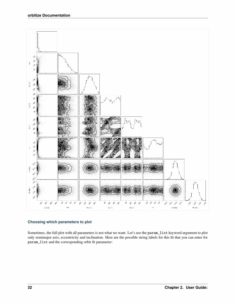
[8]: corner_figure = myResults.plot_corner()
2.2. Tutorials 31
orbitize Documentation
Choosing which parameters to plot
Sometimes, the full plot with all parameters is not what we want. Let’s use the param_list keyword argument to plotonly semimajor axis, eccentricity and inclination. Here are the possible string labels for this fit that you can enter forparam_list and the corresponding orbit fit parameter:
32 Chapter 2. User Guide:
orbitize Documentation
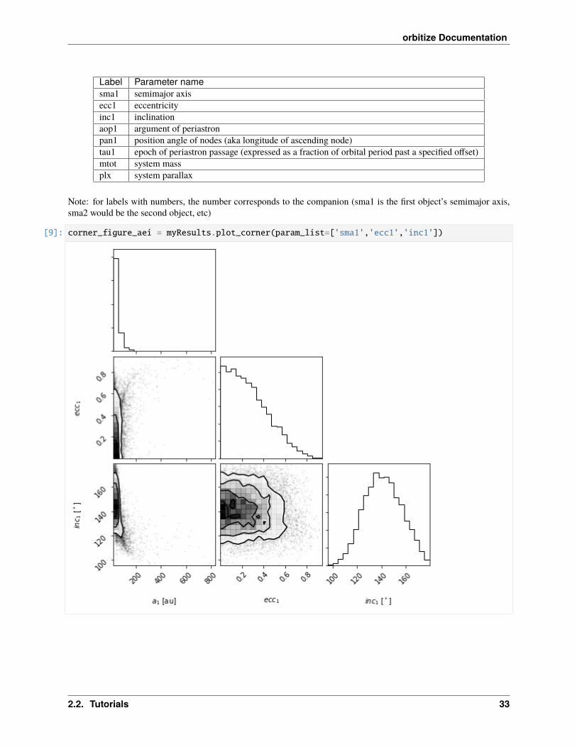
Label Parameter namesma1 semimajor axisecc1 eccentricityinc1 inclinationaop1 argument of periastronpan1 position angle of nodes (aka longitude of ascending node)tau1 epoch of periastron passage (expressed as a fraction of orbital period past a specified offset)mtot system massplx system parallax
Note: for labels with numbers, the number corresponds to the companion (sma1 is the first object’s semimajor axis,sma2 would be the second object, etc)
[9]: corner_figure_aei = myResults.plot_corner(param_list=['sma1','ecc1','inc1'])
2.2. Tutorials 33
orbitize Documentation
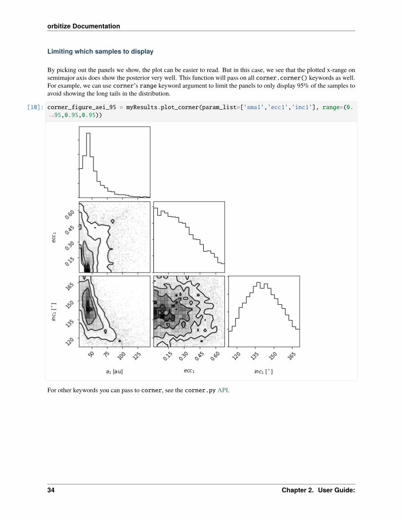
Limiting which samples to display
By picking out the panels we show, the plot can be easier to read. But in this case, we see that the plotted x-range onsemimajor axis does show the posterior very well. This function will pass on all corner.corner() keywords as well.For example, we can use corner’s range keyword argument to limit the panels to only display 95% of the samples toavoid showing the long tails in the distribution.
[10]: corner_figure_aei_95 = myResults.plot_corner(param_list=['sma1','ecc1','inc1'], range=(0.→˓95,0.95,0.95))
For other keywords you can pass to corner, see the corner.py API.
34 Chapter 2. User Guide:
orbitize Documentation
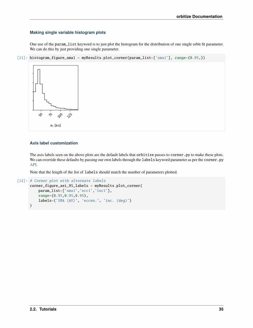
Making single variable histogram plots
One use of the param_list keyword is to just plot the histogram for the distribution of one single orbit fit parameter.We can do this by just providing one single parameter.
[11]: histogram_figure_sma1 = myResults.plot_corner(param_list=['sma1'], range=(0.95,))
Axis label customization
The axis labels seen on the above plots are the default labels that orbitize passes to corner.py to make these plots.We can override these defaults by passing our own labels through the labels keyword parameter as per the corner.pyAPI.
Note that the length of the list of labels should match the number of parameters plotted.
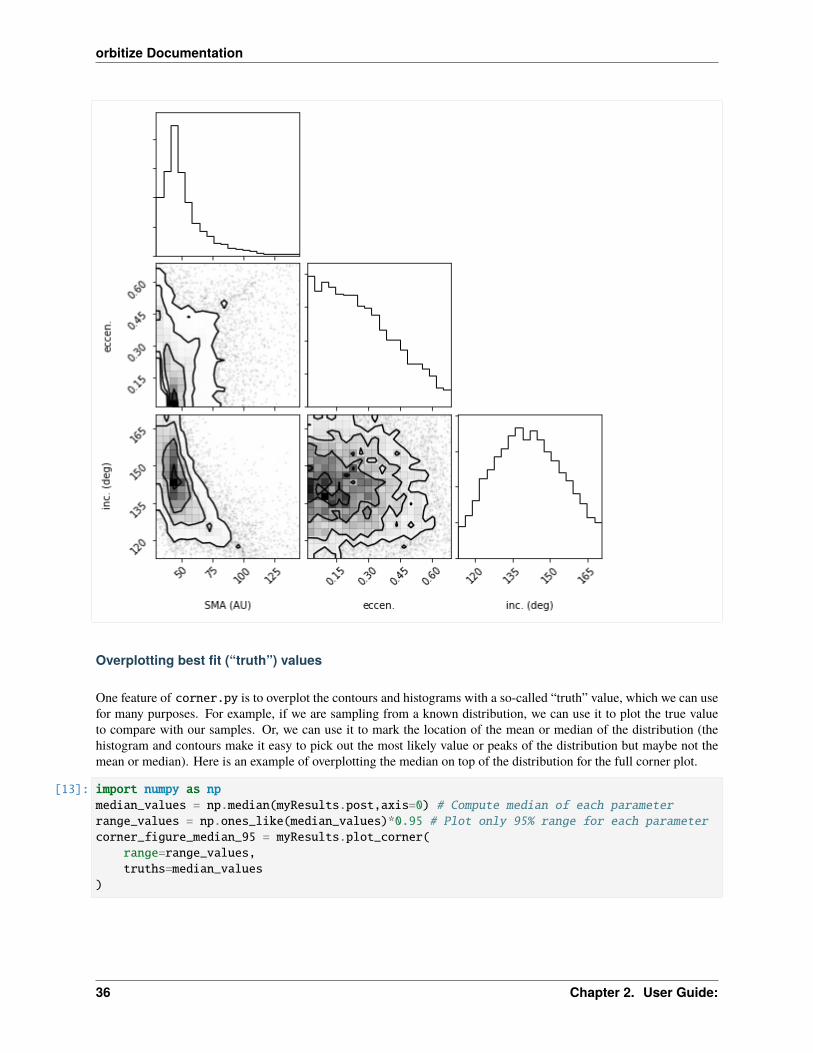
[12]: # Corner plot with alternate labelscorner_figure_aei_95_labels = myResults.plot_corner(
param_list=['sma1','ecc1','inc1'],range=(0.95,0.95,0.95),labels=('SMA (AU)', 'eccen.', 'inc. (deg)')
)
2.2. Tutorials 35
orbitize Documentation
Overplotting best fit (“truth”) values
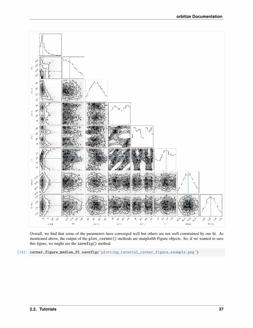
One feature of corner.py is to overplot the contours and histograms with a so-called “truth” value, which we can usefor many purposes. For example, if we are sampling from a known distribution, we can use it to plot the true valueto compare with our samples. Or, we can use it to mark the location of the mean or median of the distribution (thehistogram and contours make it easy to pick out the most likely value or peaks of the distribution but maybe not themean or median). Here is an example of overplotting the median on top of the distribution for the full corner plot.
[13]: import numpy as npmedian_values = np.median(myResults.post,axis=0) # Compute median of each parameterrange_values = np.ones_like(median_values)*0.95 # Plot only 95% range for each parametercorner_figure_median_95 = myResults.plot_corner(
range=range_values,truths=median_values
)
36 Chapter 2. User Guide:
orbitize Documentation
Overall, we find that some of the parameters have converged well but others are not well constrained by our fit. Asmentioned above, the output of the plot_corner() methods are matplotlib Figure objects. So, if we wanted to savethis figure, we might use the savefig() method.
[14]: corner_figure_median_95.savefig('plotting_tutorial_corner_figure_example.png')
2.2. Tutorials 37
orbitize Documentation
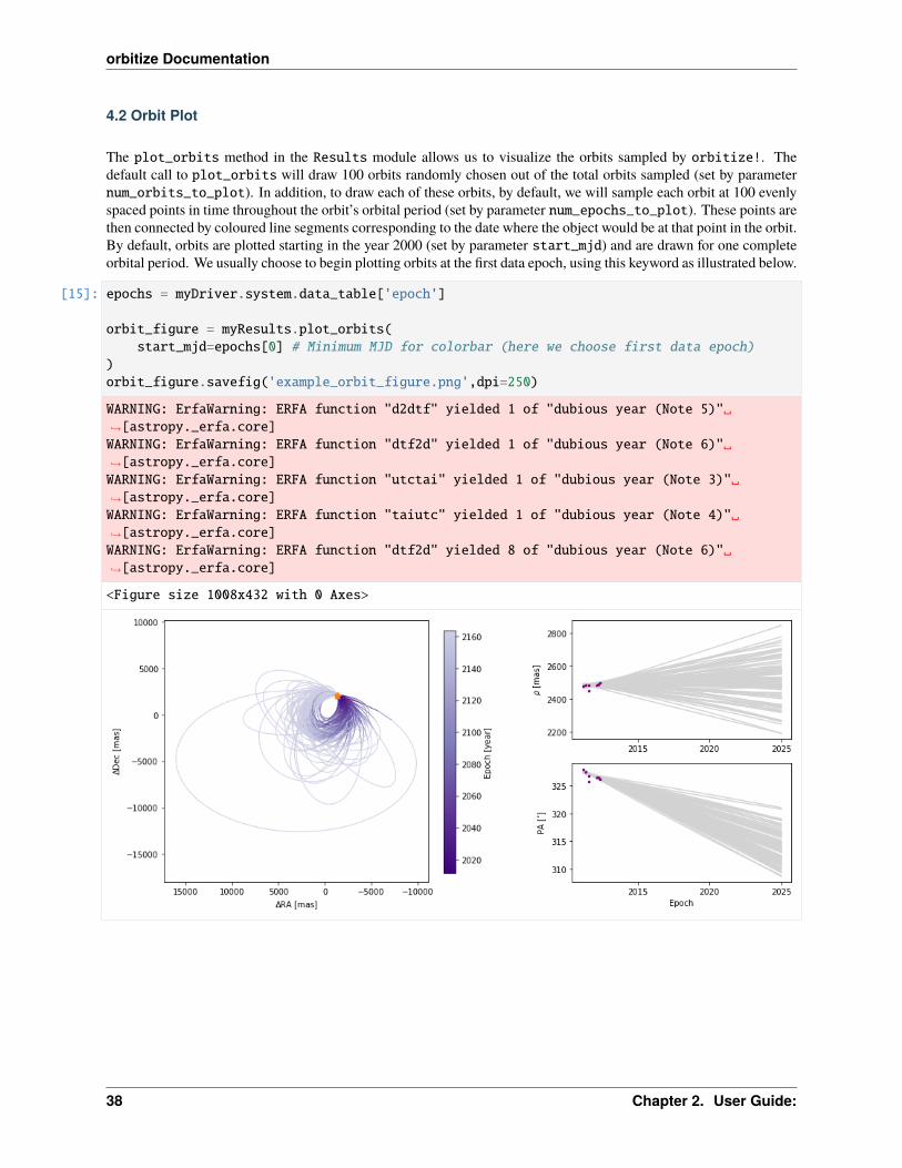
4.2 Orbit Plot
The plot_orbits method in the Results module allows us to visualize the orbits sampled by orbitize!. Thedefault call to plot_orbits will draw 100 orbits randomly chosen out of the total orbits sampled (set by parameternum_orbits_to_plot). In addition, to draw each of these orbits, by default, we will sample each orbit at 100 evenlyspaced points in time throughout the orbit’s orbital period (set by parameter num_epochs_to_plot). These points arethen connected by coloured line segments corresponding to the date where the object would be at that point in the orbit.By default, orbits are plotted starting in the year 2000 (set by parameter start_mjd) and are drawn for one completeorbital period. We usually choose to begin plotting orbits at the first data epoch, using this keyword as illustrated below.
[15]: epochs = myDriver.system.data_table['epoch']
orbit_figure = myResults.plot_orbits(start_mjd=epochs[0] # Minimum MJD for colorbar (here we choose first data epoch)
)orbit_figure.savefig('example_orbit_figure.png',dpi=250)
WARNING: ErfaWarning: ERFA function "d2dtf" yielded 1 of "dubious year (Note 5)"→˓[astropy._erfa.core]WARNING: ErfaWarning: ERFA function "dtf2d" yielded 1 of "dubious year (Note 6)"→˓[astropy._erfa.core]WARNING: ErfaWarning: ERFA function "utctai" yielded 1 of "dubious year (Note 3)"→˓[astropy._erfa.core]WARNING: ErfaWarning: ERFA function "taiutc" yielded 1 of "dubious year (Note 4)"→˓[astropy._erfa.core]WARNING: ErfaWarning: ERFA function "dtf2d" yielded 8 of "dubious year (Note 6)"→˓[astropy._erfa.core]
<Figure size 1008x432 with 0 Axes>
38 Chapter 2. User Guide:
orbitize Documentation
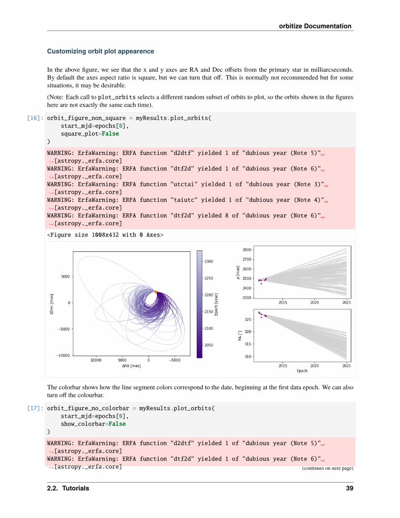
Customizing orbit plot appearence
In the above figure, we see that the x and y axes are RA and Dec offsets from the primary star in milliarcseconds.By default the axes aspect ratio is square, but we can turn that off. This is normally not recommended but for somesituations, it may be desirable.
(Note: Each call to plot_orbits selects a different random subset of orbits to plot, so the orbits shown in the figureshere are not exactly the same each time).
[16]: orbit_figure_non_square = myResults.plot_orbits(start_mjd=epochs[0],square_plot=False
)
WARNING: ErfaWarning: ERFA function "d2dtf" yielded 1 of "dubious year (Note 5)"→˓[astropy._erfa.core]WARNING: ErfaWarning: ERFA function "dtf2d" yielded 1 of "dubious year (Note 6)"→˓[astropy._erfa.core]WARNING: ErfaWarning: ERFA function "utctai" yielded 1 of "dubious year (Note 3)"→˓[astropy._erfa.core]WARNING: ErfaWarning: ERFA function "taiutc" yielded 1 of "dubious year (Note 4)"→˓[astropy._erfa.core]WARNING: ErfaWarning: ERFA function "dtf2d" yielded 8 of "dubious year (Note 6)"→˓[astropy._erfa.core]
<Figure size 1008x432 with 0 Axes>
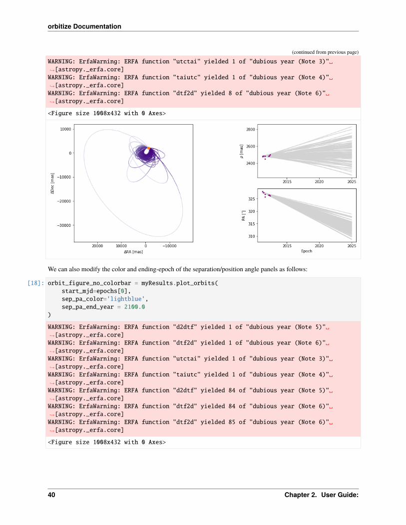
The colorbar shows how the line segment colors correspond to the date, beginning at the first data epoch. We can alsoturn off the colourbar.
[17]: orbit_figure_no_colorbar = myResults.plot_orbits(start_mjd=epochs[0],show_colorbar=False
)
WARNING: ErfaWarning: ERFA function "d2dtf" yielded 1 of "dubious year (Note 5)"→˓[astropy._erfa.core]WARNING: ErfaWarning: ERFA function "dtf2d" yielded 1 of "dubious year (Note 6)"→˓[astropy._erfa.core] (continues on next page)
2.2. Tutorials 39
orbitize Documentation
(continued from previous page)
WARNING: ErfaWarning: ERFA function "utctai" yielded 1 of "dubious year (Note 3)"→˓[astropy._erfa.core]WARNING: ErfaWarning: ERFA function "taiutc" yielded 1 of "dubious year (Note 4)"→˓[astropy._erfa.core]WARNING: ErfaWarning: ERFA function "dtf2d" yielded 8 of "dubious year (Note 6)"→˓[astropy._erfa.core]
<Figure size 1008x432 with 0 Axes>
We can also modify the color and ending-epoch of the separation/position angle panels as follows:
[18]: orbit_figure_no_colorbar = myResults.plot_orbits(start_mjd=epochs[0],sep_pa_color='lightblue',sep_pa_end_year = 2100.0
)
WARNING: ErfaWarning: ERFA function "d2dtf" yielded 1 of "dubious year (Note 5)"→˓[astropy._erfa.core]WARNING: ErfaWarning: ERFA function "dtf2d" yielded 1 of "dubious year (Note 6)"→˓[astropy._erfa.core]WARNING: ErfaWarning: ERFA function "utctai" yielded 1 of "dubious year (Note 3)"→˓[astropy._erfa.core]WARNING: ErfaWarning: ERFA function "taiutc" yielded 1 of "dubious year (Note 4)"→˓[astropy._erfa.core]WARNING: ErfaWarning: ERFA function "d2dtf" yielded 84 of "dubious year (Note 5)"→˓[astropy._erfa.core]WARNING: ErfaWarning: ERFA function "dtf2d" yielded 84 of "dubious year (Note 6)"→˓[astropy._erfa.core]WARNING: ErfaWarning: ERFA function "dtf2d" yielded 85 of "dubious year (Note 6)"→˓[astropy._erfa.core]
<Figure size 1008x432 with 0 Axes>
40 Chapter 2. User Guide:

orbitize Documentation
Choosing how orbits are plotted
Plotting one hundred orbits may be too dense. We can set the number of orbits displayed to any other value.
[19]: orbit_figure_plot10 = myResults.plot_orbits(start_mjd=epochs[0],num_orbits_to_plot=10
)
WARNING: ErfaWarning: ERFA function "d2dtf" yielded 1 of "dubious year (Note 5)"→˓[astropy._erfa.core]WARNING: ErfaWarning: ERFA function "dtf2d" yielded 1 of "dubious year (Note 6)"→˓[astropy._erfa.core]WARNING: ErfaWarning: ERFA function "utctai" yielded 1 of "dubious year (Note 3)"→˓[astropy._erfa.core]WARNING: ErfaWarning: ERFA function "taiutc" yielded 1 of "dubious year (Note 4)"→˓[astropy._erfa.core]WARNING: ErfaWarning: ERFA function "dtf2d" yielded 8 of "dubious year (Note 6)"→˓[astropy._erfa.core]
<Figure size 1008x432 with 0 Axes>
2.2. Tutorials 41
orbitize Documentation
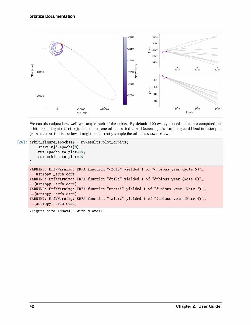
We can also adjust how well we sample each of the orbits. By default, 100 evenly-spaced points are computed perorbit, beginning at start_mjd and ending one orbital period later. Decreasing the sampling could lead to faster plotgeneration but if it is too low, it might not correctly sample the orbit, as shown below.
[20]: orbit_figure_epochs10 = myResults.plot_orbits(start_mjd=epochs[0],num_epochs_to_plot=10,num_orbits_to_plot=10
)
WARNING: ErfaWarning: ERFA function "d2dtf" yielded 1 of "dubious year (Note 5)"→˓[astropy._erfa.core]WARNING: ErfaWarning: ERFA function "dtf2d" yielded 1 of "dubious year (Note 6)"→˓[astropy._erfa.core]WARNING: ErfaWarning: ERFA function "utctai" yielded 1 of "dubious year (Note 3)"→˓[astropy._erfa.core]WARNING: ErfaWarning: ERFA function "taiutc" yielded 1 of "dubious year (Note 4)"→˓[astropy._erfa.core]
<Figure size 1008x432 with 0 Axes>
42 Chapter 2. User Guide:

orbitize Documentation
In this example, there is only one companion in orbit around the primary. When there are more than one, plot_orbitswill plot the orbits of the first companion by default and we would use the object_to_plot argument to choose adifferent object (where 1 is the first companion).
4.3 Working with matplotlib Figure objects
The idea of the Results plotting functions is to create some basic plots and to return the matplotlib Figure objectso that we can do whatever else we may want to customize the figure. We should consult the matplotlib API for allthe details. Here, we will outline a few common tasks.
Let’s increase the font sizes for all of the text (maybe for a poster or oral presentation) using matplotlib.pyplot.This (and other edits to the rcParams defaults) should be done before creating any figure objects.
[21]: plt.rcParams.update('font.size': 16)
Now, we will start with creating a figure with only 5 orbits plotted, for simplicity, with the name orb_fig. This Figureobject has two axes, one for the orbit plot and one for the colorbar. We can use the .axes property to get a list of axes.Here, we’ve named the two axes ax_orb and ax_cbar. With these three objects (orb_fig and ax_orb, and ax_cbar)we can modify all aspects of our figure.
[22]: orb_fig = myResults.plot_orbits(start_mjd=epochs[0], num_orbits_to_plot=5)ax_orb, ax_sep, ax_pa, ax_cbar = orb_fig.axes
WARNING: ErfaWarning: ERFA function "d2dtf" yielded 1 of "dubious year (Note 5)"→˓[astropy._erfa.core]WARNING: ErfaWarning: ERFA function "dtf2d" yielded 1 of "dubious year (Note 6)"→˓[astropy._erfa.core]WARNING: ErfaWarning: ERFA function "utctai" yielded 1 of "dubious year (Note 3)"→˓[astropy._erfa.core]WARNING: ErfaWarning: ERFA function "taiutc" yielded 1 of "dubious year (Note 4)"→˓[astropy._erfa.core]WARNING: ErfaWarning: ERFA function "dtf2d" yielded 8 of "dubious year (Note 6)"→˓[astropy._erfa.core]
<Figure size 1008x432 with 0 Axes>
2.2. Tutorials 43
orbitize Documentation
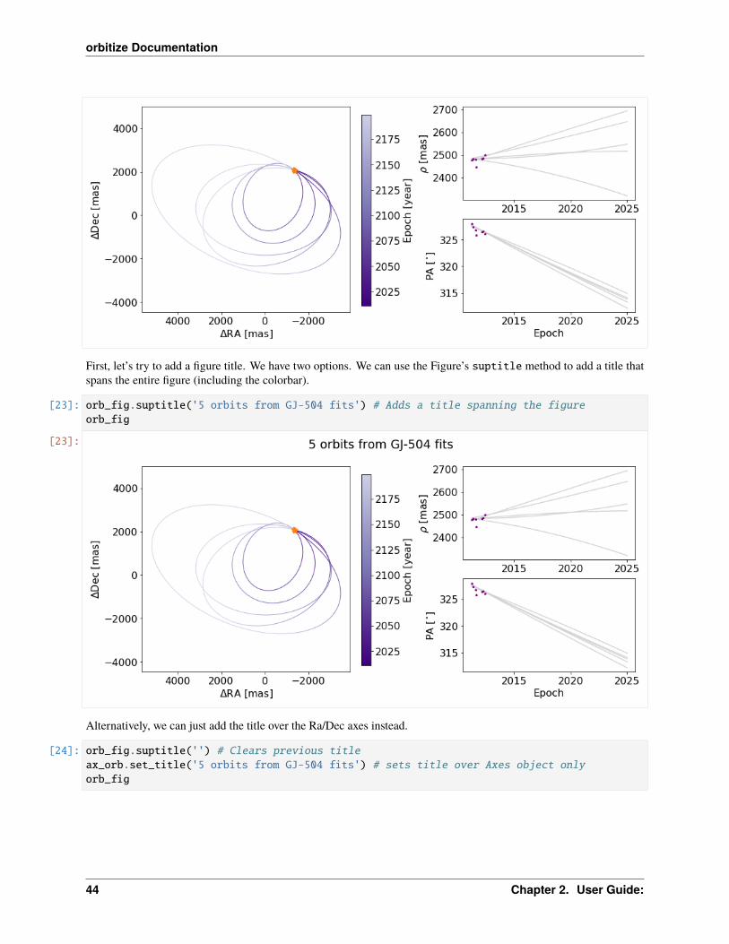
First, let’s try to add a figure title. We have two options. We can use the Figure’s suptitle method to add a title thatspans the entire figure (including the colorbar).
[23]: orb_fig.suptitle('5 orbits from GJ-504 fits') # Adds a title spanning the figureorb_fig
[23]:
Alternatively, we can just add the title over the Ra/Dec axes instead.
[24]: orb_fig.suptitle('') # Clears previous titleax_orb.set_title('5 orbits from GJ-504 fits') # sets title over Axes object onlyorb_fig
44 Chapter 2. User Guide:

orbitize Documentation
[24]:
We can also change the label of the axes, now using matplotlib.Axes methods.
[25]: ax_orb.set_xlabel('$\Delta$(Right Ascension, mas)')ax_orb.set_ylabel('$\Delta$(Declination, mas)')orb_fig
[25]:
If we want to modify the colorbar axis, we need to access the ax_cbar object
ax_orb.set_xlabel(‘∆RA [mas]’) ax_orb.set_ylabel(‘∆Dec [mas]’) # go back to what we had beforeax_cbar.set_title(‘Year’) # Put a title on the colorbar orb_fig
We may want to add to the plot itself. Here’s an exmaple of putting an star-shaped point at the location of our primarystar.
[26]: ax_orb.plot(0,0,marker="*",color='black',markersize=10)orb_fig
2.2. Tutorials 45

orbitize Documentation
[26]:
Here’s another example of adding datapoints with error bars to the separation/position angle panels:
[27]: from astropy.time import Time
# grab data from Driver objectdata_tab = myDriver.system.data_tableprint(data_tab)
epochs_yr = Time(data_tab['epoch'], format='mjd').decimalyearsep = data_tab['quant1']; sep_err = data_tab['quant1_err']pa = data_tab['quant2']; pa_err = data_tab['quant2_err']
# add data to sep panelax_sep.errorbar(
epochs_yr, sep, sep_err,color='purple', linestyle='', fmt='o', zorder=3
)
# add data to PA panelax_pa.errorbar(
epochs_yr, pa, pa_err,color='purple', linestyle='', fmt='o', zorder=3
)
# zoom in a bitax_sep.set_xlim(2011.25,2013)ax_pa.set_xlim(2011.25,2013)ax_sep.set_ylim(2450,2550)ax_pa.set_ylim(323,330)
orb_fig
epoch object quant1 quant1_err ... quant12_corr quant_type instrument(continues on next page)
46 Chapter 2. User Guide:

orbitize Documentation
(continued from previous page)
-------------- ------ ------ ---------- ... ------------ ---------- ----------55645.95 1 2479.0 16.0 ... nan seppa defsp55702.89 1 2483.0 8.0 ... nan seppa defsp55785.015 1 2481.0 33.0 ... nan seppa defsp55787.935 1 2448.0 24.0 ... nan seppa defsp
55985.19400184 1 2483.0 15.0 ... nan seppa defsp56029.11400323 1 2487.0 8.0 ... nan seppa defsp56072.30200459 1 2499.0 26.0 ... nan seppa defsp
[27]:
And finally, we can save the figure objects.
[28]: orb_fig.savefig('plotting_tutorial_plot_orbit_example.png')
2.2.7 MCMC vs OFTI Comparison
by Sarah Blunt, 2018
Welcome to the OFTI/MCMC comparison tutorial! This tutorial is meant to help you understand the differencesbetween OFTI and MCMC algorithms so you know which one to pick for your data.
Before we start, I’ll give you the short answer: for orbit fractions less than 5%, OFTI is generally faster to convergethan MCMC. This is not a hard-and-fast statistical rule, but I’ve found it to be a useful guideline.
This tutorial is essentially an abstract of Blunt et al (2017). To dig deeper, I encourage you to read the paper (Sections2.2-2.3 in particular).
Goals of This Tutorial: - Understand qualitatively why OFTI converges faster than MCMC for certain datasets. -Learn to make educated choices of backend algorithms for your own datasets.
Prerequisites: - This tutorial assumes knowledge of the orbitize API. Please go through at least the OFTI andMCMC introduction tutorials before this one. - This tutorial also assumes a qualitative understanding of OFTI andMCMC algorithms. I suggest you check out at least Section 2.1 of Blunt et al (2017) and this blog post before attemptingto decode this tutorial.
Jargon: - I will often use orbit fraction, or the fraction of the orbit spanned by the astrometric observations, as afigure of merit. In general, OFTI will converge faster than MCMC for small orbit fractions. - Convergence is defined
2.2. Tutorials 47
orbitize Documentation
differently for OFTI and for MCMC (see the OFTI paper for details). An OFTI run needs to accept a statistically largenumber of orbits for convergence, since each accepted orbit is independent of all others. For MCMC, convergenceis a bit more complicated. At a high level, an MCMC run has converged when all walkers have explored the entireparameter space. There are several metrics for estimating MCMC convergence (e.g. GR statistic, min Tz statistic), butwe’ll just estimate convergence qualitatively in this tutorial.
[1]: import numpy as npimport matplotlib.pyplot as pltimport astropy.tableimport time
from orbitize.kepler import calc_orbitfrom orbitize import system, samplerfrom orbitize.read_input import read_file
Generate Synthetic Data
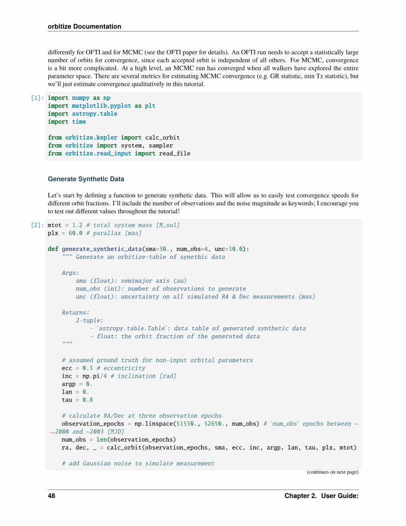
Let’s start by defining a function to generate synthetic data. This will allow us to easily test convergence speeds fordifferent orbit fractions. I’ll include the number of observations and the noise magnitude as keywords; I encourage youto test out different values throughout the tutorial!
[2]: mtot = 1.2 # total system mass [M_sol]plx = 60.0 # parallax [mas]
def generate_synthetic_data(sma=30., num_obs=4, unc=10.0):""" Generate an orbitize-table of synethic data
Args:sma (float): semimajor axis (au)num_obs (int): number of observations to generateunc (float): uncertainty on all simulated RA & Dec measurements (mas)
Returns:2-tuple:
- `astropy.table.Table`: data table of generated synthetic data- float: the orbit fraction of the generated data
"""
# assumed ground truth for non-input orbital parametersecc = 0.5 # eccentricityinc = np.pi/4 # inclination [rad]argp = 0.lan = 0.tau = 0.8
# calculate RA/Dec at three observation epochsobservation_epochs = np.linspace(51550., 52650., num_obs) # `num_obs` epochs between ~
→˓2000 and ~2003 [MJD]num_obs = len(observation_epochs)ra, dec, _ = calc_orbit(observation_epochs, sma, ecc, inc, argp, lan, tau, plx, mtot)
# add Gaussian noise to simulate measurement(continues on next page)
48 Chapter 2. User Guide:
orbitize Documentation
(continued from previous page)
ra += np.random.normal(scale=unc, size=num_obs)dec += np.random.normal(scale=unc, size=num_obs)
# define observational uncertaintiesra_err = dec_err = np.ones(num_obs)*unc
# make a plot of the dataplt.figure()plt.errorbar(ra, dec, xerr=ra_err, yerr=dec_err, linestyle='')plt.xlabel('$\\Delta$ RA'); plt.ylabel('$\\Delta$ Dec')
# calculate the orbital fractionperiod = np.sqrt((sma**3)/mtot)orbit_coverage = (max(observation_epochs) - min(observation_epochs))/365.25 # [yr]orbit_fraction = 100*orbit_coverage/period
data_table = astropy.table.Table([observation_epochs, [1]*num_obs, ra, ra_err, dec, dec_err],names=('epoch', 'object', 'raoff', 'raoff_err', 'decoff', 'decoff_err')
)# read into orbitize formatdata_table = read_file(data_table)
return data_table, orbit_fraction
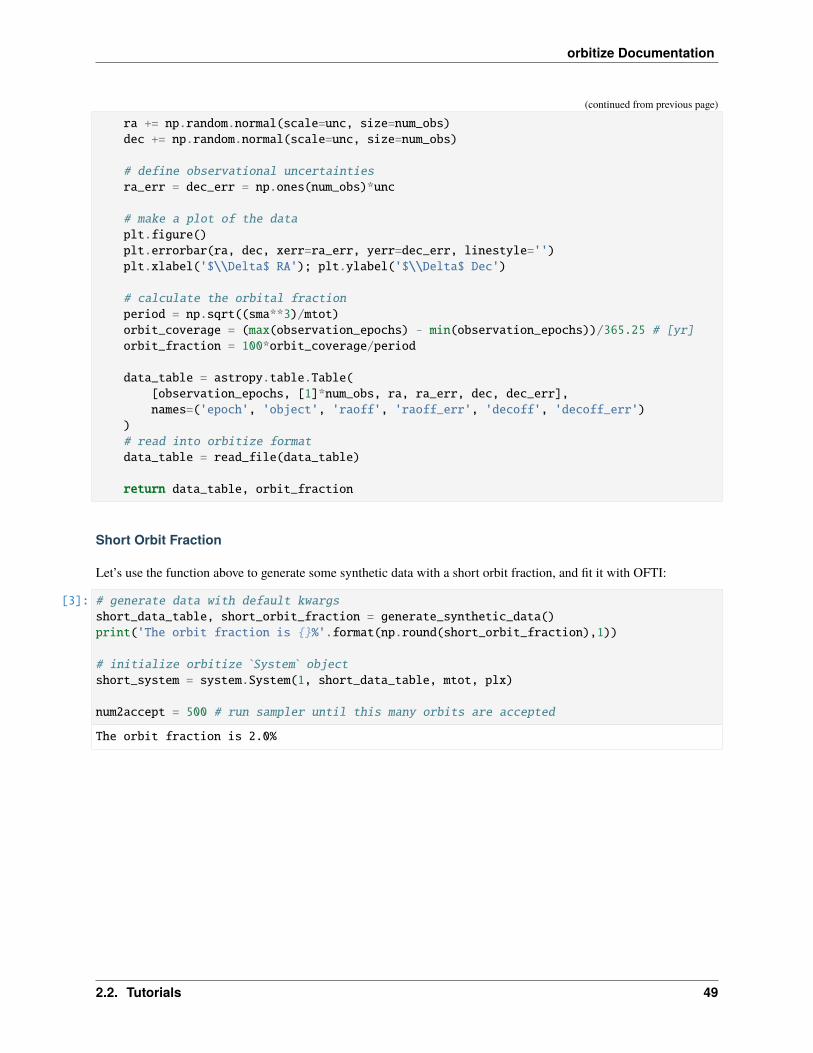
Short Orbit Fraction
Let’s use the function above to generate some synthetic data with a short orbit fraction, and fit it with OFTI:
[3]: # generate data with default kwargsshort_data_table, short_orbit_fraction = generate_synthetic_data()print('The orbit fraction is %'.format(np.round(short_orbit_fraction),1))
# initialize orbitize `System` objectshort_system = system.System(1, short_data_table, mtot, plx)
num2accept = 500 # run sampler until this many orbits are accepted
The orbit fraction is 2.0%
2.2. Tutorials 49

orbitize Documentation
[4]: start_time = time.time()
# set up OFTI `Sampler` objectshort_OFTI_sampler = sampler.OFTI(short_system)
# perform OFTI fitshort_OFTI_orbits = short_OFTI_sampler.run_sampler(num2accept)
print("OFTI took seconds to accept orbits.".format(time.time()-start_time,→˓num2accept))
Converting ra/dec data points in data_table to sep/pa. Original data are stored in input_→˓table.OFTI took 4.926873683929443 seconds to accept 500 orbits.
[5]: start_time = time.time()
# set up MCMC `Sampler` objectnum_walkers = 20short_MCMC_sampler = sampler.MCMC(short_system, num_temps=5, num_walkers=num_walkers)
# perform MCMC fitnum2accept_mcmc = 10*num2accept_ = short_MCMC_sampler.run_sampler(num2accept_mcmc, burn_steps=100)short_MCMC_orbits = short_MCMC_sampler.results.post
print("MCMC took steps in seconds.".format(num2accept_mcmc, time.time()-start_→˓time))
Starting Burn in
/home/sblunt/Projects/orbitize/orbitize/priors.py:354: RuntimeWarning: invalid value→˓encountered in loglnprob = -np.log((element_array*normalizer))
/home/sblunt/Projects/orbitize/orbitize/priors.py:463: RuntimeWarning: invalid value→˓encountered in log
(continues on next page)
50 Chapter 2. User Guide:

orbitize Documentation
(continued from previous page)
lnprob = np.log(np.sin(element_array)/normalization)
100/100 steps of burn-in completeBurn in complete. Sampling posterior now.250/250 steps completedRun completeMCMC took 5000 steps in 47.53257179260254 seconds.
[6]: plt.hist(short_OFTI_orbits[:, short_system.param_idx['ecc1']], bins=40, density=True,→˓alpha=.5, label='OFTI')plt.hist(short_MCMC_orbits[:, short_system.param_idx['ecc1']], bins=40, density=True,→˓alpha=.5, label='MCMC')
plt.xlabel('Eccentricity'); plt.ylabel('Prob.')plt.legend()
[6]: <matplotlib.legend.Legend at 0x7f1506e50d90>
These distributions are different because the MCMC chains have not converged, resulting in a “lumpy” MCMC dis-tribution. I set up the calculation so that MCMC would return 10x as many orbits as OFTI, but even so, the OFTIdistribution is a much better representation of the underlying PDF.
If we run the MCMC algorithm for a greater number of steps (and/or increase the number of walkers and/or tempera-tures), the MCMC and OFTI distributions will become indistinguishable. OFTI is NOT more correct than MCMC,but for this dataset, OFTI converges on the correct posterior faster than MCMC.
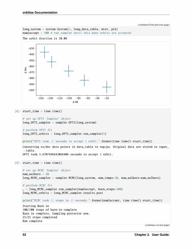
Longer Orbit Fraction
Let’s now repeat this exercise with a longer orbit fraction. For this dataset, OFTI will have to run for several secondsjust to accept one orbit, so we won’t compare the resulting posteriors.
[7]: # generate datalong_data_table, long_orbit_fraction = generate_synthetic_data(sma=10, num_obs=5)print('The orbit fraction is %'.format(np.round(long_orbit_fraction),1))
# initialize orbitize `System` object(continues on next page)
2.2. Tutorials 51
orbitize Documentation
(continued from previous page)
long_system = system.System(1, long_data_table, mtot, plx)num2accept = 500 # run sampler until this many orbits are accepted
The orbit fraction is 10.0%
[8]: start_time = time.time()
# set up OFTI `Sampler` objectlong_OFTI_sampler = sampler.OFTI(long_system)
# perform OFTI fitlong_OFTI_orbits = long_OFTI_sampler.run_sampler(1)
print("OFTI took seconds to accept 1 orbit.".format(time.time()-start_time))
Converting ra/dec data points in data_table to sep/pa. Original data are stored in input_→˓table.OFTI took 3.6707496643066406 seconds to accept 1 orbit.
[9]: start_time = time.time()
# set up MCMC `Sampler` objectnum_walkers = 20long_MCMC_sampler = sampler.MCMC(long_system, num_temps=10, num_walkers=num_walkers)
# perform MCMC fit_ = long_MCMC_sampler.run_sampler(num2accept, burn_steps=100)long_MCMC_orbits = long_MCMC_sampler.results.post
print("MCMC took steps in seconds.".format(num2accept, time.time()-start_time))
Starting Burn in100/100 steps of burn-in completeBurn in complete. Sampling posterior now.25/25 steps completedRun complete
(continues on next page)
52 Chapter 2. User Guide:
orbitize Documentation
(continued from previous page)
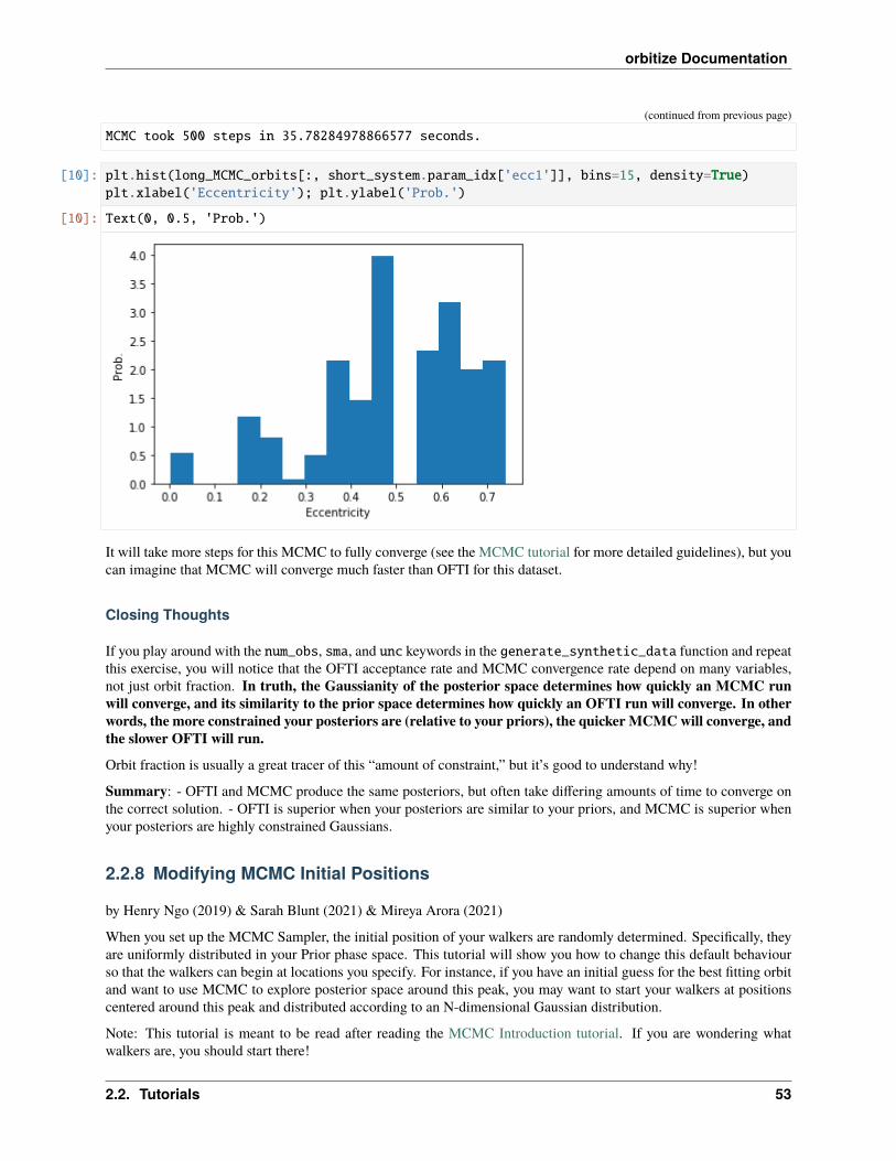
MCMC took 500 steps in 35.78284978866577 seconds.
[10]: plt.hist(long_MCMC_orbits[:, short_system.param_idx['ecc1']], bins=15, density=True)plt.xlabel('Eccentricity'); plt.ylabel('Prob.')
[10]: Text(0, 0.5, 'Prob.')
It will take more steps for this MCMC to fully converge (see the MCMC tutorial for more detailed guidelines), but youcan imagine that MCMC will converge much faster than OFTI for this dataset.
Closing Thoughts
If you play around with the num_obs, sma, and unc keywords in the generate_synthetic_data function and repeatthis exercise, you will notice that the OFTI acceptance rate and MCMC convergence rate depend on many variables,not just orbit fraction. In truth, the Gaussianity of the posterior space determines how quickly an MCMC runwill converge, and its similarity to the prior space determines how quickly an OFTI run will converge. In otherwords, the more constrained your posteriors are (relative to your priors), the quicker MCMC will converge, andthe slower OFTI will run.
Orbit fraction is usually a great tracer of this “amount of constraint,” but it’s good to understand why!
Summary: - OFTI and MCMC produce the same posteriors, but often take differing amounts of time to converge onthe correct solution. - OFTI is superior when your posteriors are similar to your priors, and MCMC is superior whenyour posteriors are highly constrained Gaussians.
2.2.8 Modifying MCMC Initial Positions
by Henry Ngo (2019) & Sarah Blunt (2021) & Mireya Arora (2021)
When you set up the MCMC Sampler, the initial position of your walkers are randomly determined. Specifically, theyare uniformly distributed in your Prior phase space. This tutorial will show you how to change this default behaviourso that the walkers can begin at locations you specify. For instance, if you have an initial guess for the best fitting orbitand want to use MCMC to explore posterior space around this peak, you may want to start your walkers at positionscentered around this peak and distributed according to an N-dimensional Gaussian distribution.
Note: This tutorial is meant to be read after reading the MCMC Introduction tutorial. If you are wondering whatwalkers are, you should start there!
2.2. Tutorials 53
orbitize Documentation
The Driver class is the main way you might interact with orbitize! as it automatically reads your input, creates allthe orbitize! objects needed to do your calculation, and defaults to some commonly used parameters or settings.However, sometimes you want to work directly with the underlying API to do more advanced tasks such as changingthe MCMC walkers’ initial positions, or modifying the priors.
This tutorial walks you through how to do that.
Goals of this tutorial: - Learn to modify the MCMC Sampler object - Learn about the structure of the orbitizecode base
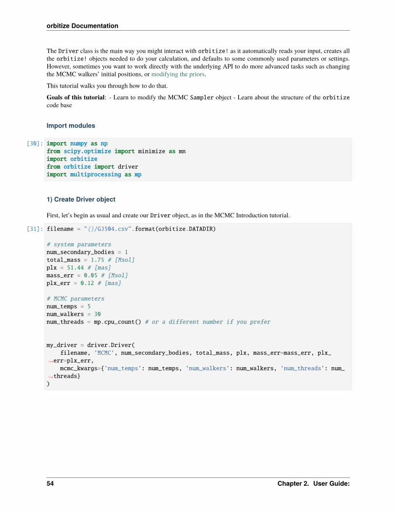
Import modules
[30]: import numpy as npfrom scipy.optimize import minimize as mnimport orbitizefrom orbitize import driverimport multiprocessing as mp
1) Create Driver object
First, let’s begin as usual and create our Driver object, as in the MCMC Introduction tutorial.
[31]: filename = "/GJ504.csv".format(orbitize.DATADIR)
# system parametersnum_secondary_bodies = 1total_mass = 1.75 # [Msol]plx = 51.44 # [mas]mass_err = 0.05 # [Msol]plx_err = 0.12 # [mas]
# MCMC parametersnum_temps = 5num_walkers = 30num_threads = mp.cpu_count() # or a different number if you prefer
my_driver = driver.Driver(filename, 'MCMC', num_secondary_bodies, total_mass, plx, mass_err=mass_err, plx_
→˓err=plx_err,mcmc_kwargs='num_temps': num_temps, 'num_walkers': num_walkers, 'num_threads': num_
→˓threads)
54 Chapter 2. User Guide:

orbitize Documentation
2) Access the Sampler object to view the walker positions
As mentioned in the introduction, the Driver class creates the objects needed for the orbit fit. At the time of thiswriting, it creates a Sampler object which you can access with the .sampler attribute and a System object which youcan access with the .system attribute.
The Sampler object contains all of the information used by the orbit sampling algorithm (OFTI or MCMC) to fitthe orbit and determine the posteriors. The System object contains information about the astrophysical system itself(stellar and companion parameters, the input data, etc.).
To see all of the attributes of the driver object, you can use dir().
[32]: print(dir(my_driver))
['__class__', '__delattr__', '__dict__', '__dir__', '__doc__', '__eq__', '__format__', '_→˓_ge__', '__getattribute__', '__gt__', '__hash__', '__init__', '__init_subclass__', '__→˓le__', '__lt__', '__module__', '__ne__', '__new__', '__reduce__', '__reduce_ex__', '__→˓repr__', '__setattr__', '__sizeof__', '__str__', '__subclasshook__', '__weakref__',→˓'sampler', 'system']
This returns many other functions too, but you see sampler and system at the bottom. Don’t forget that in Jupyternotebooks, you can use my_driver? to get the docstring for its class (i.e. the Driver class) and my_driver?? to getthe full source code of that class. You can also get this information in the API documentation.
Now, let’s list the attributes of the my_driver.sampler attribute.
[33]: print(dir(my_driver.sampler))
['__abstractmethods__', '__class__', '__delattr__', '__dict__', '__dir__', '__doc__', '__→˓eq__', '__format__', '__ge__', '__getattribute__', '__gt__', '__hash__', '__init__', '_→˓_init_subclass__', '__le__', '__lt__', '__module__', '__ne__', '__new__', '__reduce__',→˓ '__reduce_ex__', '__repr__', '__setattr__', '__sizeof__', '__slotnames__', '__slots__→˓', '__str__', '__subclasshook__', '__weakref__', '_abc_impl', '_fill_in_fixed_params',→˓'_logl', '_update_chains_from_sampler', 'check_prior_support', 'chop_chains', 'curr_pos→˓', 'custom_lnlike', 'examine_chains', 'fixed_params', 'has_corr', 'lnlike', 'num_params→˓', 'num_temps', 'num_threads', 'num_walkers', 'priors', 'results', 'run_sampler',→˓'sampled_param_idx', 'system', 'use_pt', 'validate_xyz_positions']
Again, you can use the ? and ?? features as well as the API documentation to find out more. Here we see an attributecurr_poswhich contains the current position of all the walkers for the MCMC sampler. These positions were generatedupon initialization of the Sampler object, which happened as part of the initialization of the Driver object.
Examine my_driver.sampler.curr_pos
curr_pos is an array and has shape (n_temps, n_walkers, n_params) for the parallel-tempered MCMC sampler andshape (n_walkers, n_params) for the affine-invariant ensemble sampler.
[34]: my_driver.sampler.curr_pos.shape # Here we are using the parallel-tempered MCMC sampler
[34]: (5, 30, 8)
Basically, this is the same shape as the output of the Sampler. Let’s look at the start position of the first five walkers atthe lowest temperature, to get a better sense of what the strucutre is like.
[35]: print(my_driver.sampler.curr_pos[0,0:5,:])
2.2. Tutorials 55
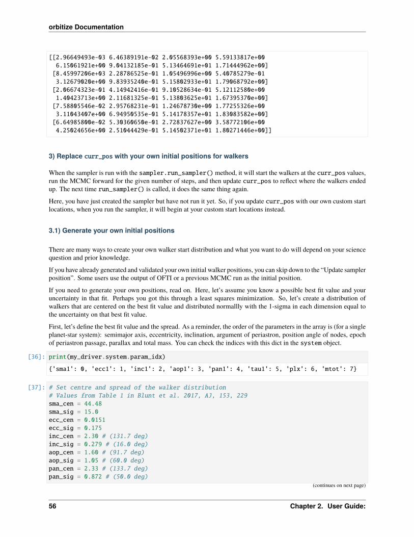
orbitize Documentation
[[2.96649493e-03 6.46389191e-02 2.05568393e+00 5.59133817e+006.15061921e+00 9.04132185e-01 5.13464691e+01 1.71444962e+00]
[8.45997206e+03 2.28786525e-01 1.05496996e+00 5.40785279e-013.12679020e+00 9.83935240e-01 5.15802933e+01 1.79068792e+00]
[2.06674323e-01 4.14942416e-01 9.10528634e-01 5.12112580e+001.40423713e+00 2.11681325e-01 5.13803625e+01 1.67395370e+00]
[7.58805546e-02 2.95768231e-01 1.24678730e+00 1.77255326e+003.11043407e+00 6.94950535e-01 5.14178357e+01 1.83083582e+00]
[6.64985800e-02 5.30360650e-01 2.72837627e+00 3.58772106e+004.25024656e+00 2.51044429e-01 5.14502371e+01 1.80271446e+00]]
3) Replace curr_pos with your own initial positions for walkers
When the sampler is run with the sampler.run_sampler() method, it will start the walkers at the curr_pos values,run the MCMC forward for the given number of steps, and then update curr_pos to reflect where the walkers endedup. The next time run_sampler() is called, it does the same thing again.
Here, you have just created the sampler but have not run it yet. So, if you update curr_pos with our own custom startlocations, when you run the sampler, it will begin at your custom start locations instead.
3.1) Generate your own initial positions
There are many ways to create your own walker start distribution and what you want to do will depend on your sciencequestion and prior knowledge.
If you have already generated and validated your own initial walker positions, you can skip down to the “Update samplerposition”. Some users use the output of OFTI or a previous MCMC run as the initial position.
If you need to generate your own positions, read on. Here, let’s assume you know a possible best fit value and youruncertainty in that fit. Perhaps you got this through a least squares minimization. So, let’s create a distribution ofwalkers that are centered on the best fit value and distributed normallly with the 1-sigma in each dimension equal tothe uncertainty on that best fit value.
First, let’s define the best fit value and the spread. As a reminder, the order of the parameters in the array is (for a singleplanet-star system): semimajor axis, eccentricity, inclination, argument of periastron, position angle of nodes, epochof periastron passage, parallax and total mass. You can check the indices with this dict in the system object.
[36]: print(my_driver.system.param_idx)
'sma1': 0, 'ecc1': 1, 'inc1': 2, 'aop1': 3, 'pan1': 4, 'tau1': 5, 'plx': 6, 'mtot': 7
[37]: # Set centre and spread of the walker distribution# Values from Table 1 in Blunt et al. 2017, AJ, 153, 229sma_cen = 44.48sma_sig = 15.0ecc_cen = 0.0151ecc_sig = 0.175inc_cen = 2.30 # (131.7 deg)inc_sig = 0.279 # (16.0 deg)aop_cen = 1.60 # (91.7 deg)aop_sig = 1.05 # (60.0 deg)pan_cen = 2.33 # (133.7 deg)pan_sig = 0.872 # (50.0 deg)
(continues on next page)
56 Chapter 2. User Guide:
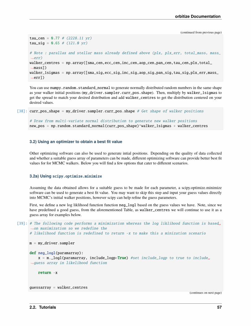
orbitize Documentation
(continued from previous page)
tau_cen = 0.77 # (2228.11 yr)tau_sig = 0.65 # (121.0 yr)
# Note : parallax and stellar mass already defined above (plx, plx_err, total_mass, mass_→˓err)walker_centres = np.array([sma_cen,ecc_cen,inc_cen,aop_cen,pan_cen,tau_cen,plx,total_→˓mass])walker_1sigmas = np.array([sma_sig,ecc_sig,inc_sig,aop_sig,pan_sig,tau_sig,plx_err,mass_→˓err])
You can use numpy.random.standard_normal to generate normally distributed random numbers in the same shapeas your walker initial positions (my_driver.sampler.curr_pos.shape). Then, multiply by walker_1sigmas toget the spread to match your desired distribution and add walker_centres to get the distribution centered on yourdesired values.
[38]: curr_pos_shape = my_driver.sampler.curr_pos.shape # Get shape of walker positions
# Draw from multi-variate normal distribution to generate new walker positionsnew_pos = np.random.standard_normal(curr_pos_shape)*walker_1sigmas + walker_centres
3.2) Using an optimizer to obtain a best fit value
Other optimizing software can also be used to generate intial positions. Depending on the quality of data collectedand whether a suitable guess array of parameters can be made, different optimizing software can provide better best fitvalues for for MCMC walkers. Below you will find a few options that cater to different scenarios.
3.2a) Using scipy.optimize.minimize
Assuming the data obtained allows for a suitable guess to be made for each parameter, a scipy.optimize.minimizesoftware can be used to generate a best fit value. You may want to skip this step and input your guess values directlyinto MCMC’s initial walker positions, however scipy can help refine the guess parameters.
First, we define a new log liklihood function function neg_logl based on the guess values we have. Note, since wehave predefined a good guess, from the aforementioned Table, as walker_centres we will continue to use it as aguess array for examples below.
[39]: # The following code performs a minimization whereas the log liklihood function is based→˓on maximization so we redefine the# likelihood function is redefined to return -x to make this a minization scenario
m = my_driver.sampler
def neg_logl(paramarray):x = m._logl(paramarray, include_logp=True) #set include_logp to true to include
→˓guess array in likelihood function
return -x
guessarray = walker_centres(continues on next page)
2.2. Tutorials 57

orbitize Documentation
(continued from previous page)
results = mn(neg_logl, guessarray, method="Powell")print(results.x) #results.x is the best fit value
[4.90426906e+01 9.99455386e-06 2.48501010e+00 1.60085022e+002.33034111e+00 7.69934177e-01 5.14404237e+01 1.74922411e+00]
In our trials, Powell has given the best results, but you may replace it with a different minimizing method dependingon your need.
3.3) Scattering walkers
To set up MCMC so that it explores the nearby probablity space thoroughly and finds the global minimum, you canscatter the initial positions of the walkers around the best fit value. This can be done by adding random numbers toresults.x
This section overrides walker_1sigmas and creates a spread of new_pos in a different manner than above. The followingis a template based on the aforementioned Table. The scatter is created using a variety of methods, we recommendreviewing the code to ensure it is compatible to your data.
[40]: new_pos = np.random.standard_normal(curr_pos_shape)*0.03 + results.x
3.4) Update sampler position
After generating and validating your new walker positions, through whatever methods you choose, it’s now time toupdate the sampler object to have its curr_pos be your new positions.
[41]: my_driver.sampler.curr_pos = np.copy(new_pos)
3.5) Validate your new positions
Drawing from a normal distribution can cause your walkers to start outside of your prior space. See the ModifyingPriors tutorial for information on how to interact with the prior objects, which would allow you to find the limits oneach parameter set by the priors etc.
Here, let’s do something more simple and just check that all values are physically valid. After this we can begin tocorrect them.
The following function can be used to identify walkers that have been initialized outside of the appropriate prior proba-bility space. It will raise a ValueError if walkers are initialized outside of the priors. You should update your positionsuntil this method runs without raising an error.
[42]: my_driver.sampler.check_prior_support()
---------------------------------------------------------------------------ValueError Traceback (most recent call last)<ipython-input-42-1b66a275c5b0> in <module>----> 1 my_driver.sampler.check_prior_support()
~/Projects/orbitize/orbitize/sampler.py in check_prior_support(self)1094 # Throw our ValueError if necessary,1095 if len(bad_parameters) > 0:
(continues on next page)
58 Chapter 2. User Guide:
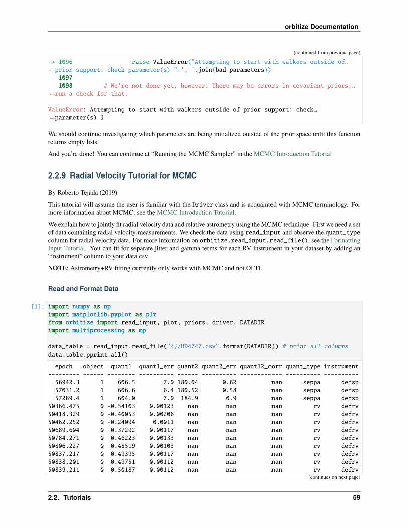
orbitize Documentation
(continued from previous page)
-> 1096 raise ValueError("Attempting to start with walkers outside of→˓prior support: check parameter(s) "+', '.join(bad_parameters))10971098 # We're not done yet, however. There may be errors in covariant priors;
→˓run a check for that.
ValueError: Attempting to start with walkers outside of prior support: check→˓parameter(s) 1
We should continue investigating which parameters are being initialized outside of the prior space until this functionreturns empty lists.
And you’re done! You can continue at “Running the MCMC Sampler” in the MCMC Introduction Tutorial
2.2.9 Radial Velocity Tutorial for MCMC
By Roberto Tejada (2019)
This tutorial will assume the user is familiar with the Driver class and is acquainted with MCMC terminology. Formore information about MCMC, see the MCMC Introduction Tutorial.
We explain how to jointly fit radial velocity data and relative astrometry using the MCMC technique. First we need a setof data containing radial velocity measurements. We check the data using read_input and observe the quant_typecolumn for radial velocity data. For more information on orbitize.read_input.read_file(), see the FormattingInput Tutorial. You can fit for separate jitter and gamma terms for each RV instrument in your dataset by adding an“instrument” column to your data csv.
NOTE: Astrometry+RV fitting currently only works with MCMC and not OFTI.
Read and Format Data
[1]: import numpy as npimport matplotlib.pyplot as pltfrom orbitize import read_input, plot, priors, driver, DATADIRimport multiprocessing as mp
data_table = read_input.read_file("/HD4747.csv".format(DATADIR)) # print all columnsdata_table.pprint_all()
epoch object quant1 quant1_err quant2 quant2_err quant12_corr quant_type instrument--------- ------ -------- ---------- ------ ---------- ------------ ---------- ----------56942.3 1 606.5 7.0 180.04 0.62 nan seppa defsp57031.2 1 606.6 6.4 180.52 0.58 nan seppa defsp57289.4 1 604.0 7.0 184.9 0.9 nan seppa defsp
50366.475 0 -0.54103 0.00123 nan nan nan rv defrv50418.329 0 -0.40053 0.00206 nan nan nan rv defrv50462.252 0 -0.24094 0.0011 nan nan nan rv defrv50689.604 0 0.37292 0.00117 nan nan nan rv defrv50784.271 0 0.46223 0.00133 nan nan nan rv defrv50806.227 0 0.48519 0.00103 nan nan nan rv defrv50837.217 0 0.49395 0.00117 nan nan nan rv defrv50838.201 0 0.49751 0.00112 nan nan nan rv defrv50839.211 0 0.50187 0.00112 nan nan nan rv defrv
(continues on next page)
2.2. Tutorials 59
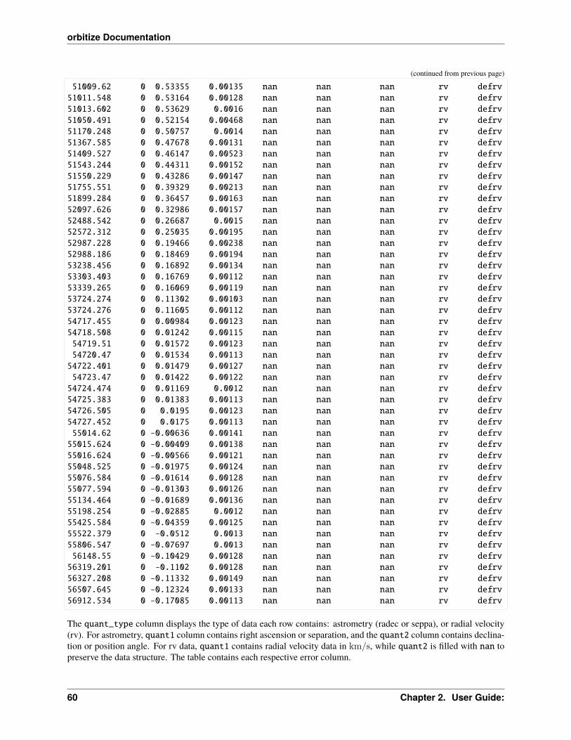
orbitize Documentation
(continued from previous page)
51009.62 0 0.53355 0.00135 nan nan nan rv defrv51011.548 0 0.53164 0.00128 nan nan nan rv defrv51013.602 0 0.53629 0.0016 nan nan nan rv defrv51050.491 0 0.52154 0.00468 nan nan nan rv defrv51170.248 0 0.50757 0.0014 nan nan nan rv defrv51367.585 0 0.47678 0.00131 nan nan nan rv defrv51409.527 0 0.46147 0.00523 nan nan nan rv defrv51543.244 0 0.44311 0.00152 nan nan nan rv defrv51550.229 0 0.43286 0.00147 nan nan nan rv defrv51755.551 0 0.39329 0.00213 nan nan nan rv defrv51899.284 0 0.36457 0.00163 nan nan nan rv defrv52097.626 0 0.32986 0.00157 nan nan nan rv defrv52488.542 0 0.26687 0.0015 nan nan nan rv defrv52572.312 0 0.25035 0.00195 nan nan nan rv defrv52987.228 0 0.19466 0.00238 nan nan nan rv defrv52988.186 0 0.18469 0.00194 nan nan nan rv defrv53238.456 0 0.16892 0.00134 nan nan nan rv defrv53303.403 0 0.16769 0.00112 nan nan nan rv defrv53339.265 0 0.16069 0.00119 nan nan nan rv defrv53724.274 0 0.11302 0.00103 nan nan nan rv defrv53724.276 0 0.11605 0.00112 nan nan nan rv defrv54717.455 0 0.00984 0.00123 nan nan nan rv defrv54718.508 0 0.01242 0.00115 nan nan nan rv defrv54719.51 0 0.01572 0.00123 nan nan nan rv defrv54720.47 0 0.01534 0.00113 nan nan nan rv defrv54722.401 0 0.01479 0.00127 nan nan nan rv defrv54723.47 0 0.01422 0.00122 nan nan nan rv defrv54724.474 0 0.01169 0.0012 nan nan nan rv defrv54725.383 0 0.01383 0.00113 nan nan nan rv defrv54726.505 0 0.0195 0.00123 nan nan nan rv defrv54727.452 0 0.0175 0.00113 nan nan nan rv defrv55014.62 0 -0.00636 0.00141 nan nan nan rv defrv55015.624 0 -0.00409 0.00138 nan nan nan rv defrv55016.624 0 -0.00566 0.00121 nan nan nan rv defrv55048.525 0 -0.01975 0.00124 nan nan nan rv defrv55076.584 0 -0.01614 0.00128 nan nan nan rv defrv55077.594 0 -0.01303 0.00126 nan nan nan rv defrv55134.464 0 -0.01689 0.00136 nan nan nan rv defrv55198.254 0 -0.02885 0.0012 nan nan nan rv defrv55425.584 0 -0.04359 0.00125 nan nan nan rv defrv55522.379 0 -0.0512 0.0013 nan nan nan rv defrv55806.547 0 -0.07697 0.0013 nan nan nan rv defrv56148.55 0 -0.10429 0.00128 nan nan nan rv defrv56319.201 0 -0.1102 0.00128 nan nan nan rv defrv56327.208 0 -0.11332 0.00149 nan nan nan rv defrv56507.645 0 -0.12324 0.00133 nan nan nan rv defrv56912.534 0 -0.17085 0.00113 nan nan nan rv defrv
The quant_type column displays the type of data each row contains: astrometry (radec or seppa), or radial velocity(rv). For astrometry, quant1 column contains right ascension or separation, and the quant2 column contains declina-tion or position angle. For rv data, quant1 contains radial velocity data in km/s, while quant2 is filled with nan topreserve the data structure. The table contains each respective error column.
60 Chapter 2. User Guide:
orbitize Documentation
We can now initialize the Driver class. MCMC samplers take time to converge to absolute maxima in parameterspace, and the more parameters we introduce, the longer we expect it to take.
Create Driver Object
For joint orbital fits with RV data, we need to fit the stellar and companion masses (m0 and m1 respectively as separatefree parameters). This differs from the astrometry-only case where fitting the total mass mtot suffices. We set thesystem keyword fit_secondary_mass to True when initializing the Driver object.
[2]: filename = "/HD4747.csv".format(DATADIR)
# system parametersnum_secondary_bodies = 1stellar_mass = 0.84 # [Msol]plx = 53.18 # [mas]mass_err = 0.04 # [Msol]plx_err = 0.12 # [mas]
# MCMC parametersnum_temps = 5num_walkers = 30num_threads = 2 # or a different number if you prefer, eg mp.cpu_count()
my_driver = driver.Driver(filename, 'MCMC', num_secondary_bodies, stellar_mass, plx, mass_err=mass_err, plx_
→˓err=plx_err,system_kwargs = 'fit_secondary_mass':True, 'tau_ref_epoch':0,mcmc_kwargs='num_temps': num_temps, 'num_walkers': num_walkers, 'num_threads': num_
→˓threads)
Since MCMC is an object in orbitize!, we can assign a variable to the sampler and work with this variable:
[3]: m = my_driver.sampler
RV Priors
The priors for the two RV parameters, the radial velocity offset (gamma), and jitter (sigma), have default uniform priorand log uniform prior respectively. The gamma uniform prior is set between (−5, 5) km/s, and the jitter log uniformprior is set for (10−4, 0.05) km/s. The prior for m1 is a log uniform prior and is set for (10−3, 2.0)𝑀⊙. The currentversion of orbitize addressed in this tutorial returns the stellar radial velocity only.
NOTE: We may change the priors as instructed in the Modifying Priors tutorial:
[4]: # getting the system object:sys = my_driver.system
lab = sys.param_idx
print(sys.labels)print(sys.sys_priors)
print(vars(sys.sys_priors[lab['m1']]))
2.2. Tutorials 61
orbitize Documentation
['sma1', 'ecc1', 'inc1', 'aop1', 'pan1', 'tau1', 'plx', 'gamma_defrv', 'sigma_defrv', 'm1→˓', 'm0'][Log Uniform, Uniform, Sine, Uniform, Uniform, Uniform, Gaussian, Uniform, Log Uniform,→˓Log Uniform, Gaussian]'minval': 1e-06, 'maxval': 2, 'logmin': -13.815510557964274, 'logmax': 0.→˓6931471805599453
[5]: # change the m1 prior:sys.sys_priors[lab['m1']] = priors.LogUniformPrior(1e-4, 0.5)
print(sys.labels)print(sys.sys_priors)print(vars(sys.sys_priors[lab['m1']]))
['sma1', 'ecc1', 'inc1', 'aop1', 'pan1', 'tau1', 'plx', 'gamma_defrv', 'sigma_defrv', 'm1→˓', 'm0'][Log Uniform, Uniform, Sine, Uniform, Uniform, Uniform, Gaussian, Uniform, Log Uniform,→˓Log Uniform, Gaussian]'minval': 0.0001, 'maxval': 0.5, 'logmin': -9.210340371976182, 'logmax': -0.→˓6931471805599453
Running the MCMC Sampler
As noted in the MCMC Introduction Tutorial, we must choose the sampler step for MCMC and can save every 𝑛𝑡ℎsample to avoid using too much disk space using thin.
[6]: total_orbits = 1000 # number of steps x number of walkers (at lowest temperature)burn_steps = 10 # steps to burn in per walkerthin = 2 # only save every 2 steps
[7]: m.run_sampler(total_orbits, burn_steps=burn_steps, thin=thin)
Starting Burn in
/home/sblunt/Projects/orbitize/orbitize/priors.py:354: RuntimeWarning: invalid value→˓encountered in loglnprob = -np.log((element_array*normalizer))
/home/sblunt/Projects/orbitize/orbitize/priors.py:354: RuntimeWarning: invalid value→˓encountered in loglnprob = -np.log((element_array*normalizer))
/home/sblunt/Projects/orbitize/orbitize/priors.py:463: RuntimeWarning: invalid value→˓encountered in loglnprob = np.log(np.sin(element_array)/normalization)
/home/sblunt/Projects/orbitize/orbitize/priors.py:463: RuntimeWarning: invalid value→˓encountered in loglnprob = np.log(np.sin(element_array)/normalization)
10/10 steps of burn-in completeBurn in complete. Sampling posterior now.
Run complete
[7]: <ptemcee.sampler.Sampler at 0x7f17c0d19b50>
62 Chapter 2. User Guide:
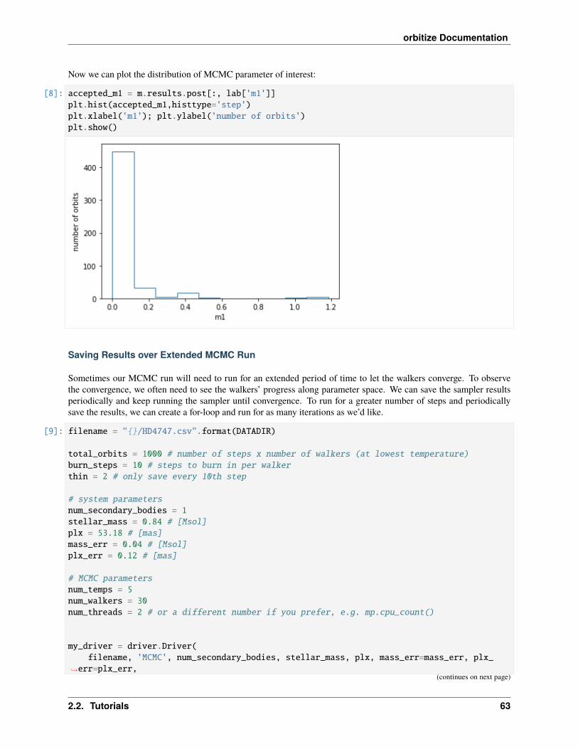
orbitize Documentation
Now we can plot the distribution of MCMC parameter of interest:
[8]: accepted_m1 = m.results.post[:, lab['m1']]plt.hist(accepted_m1,histtype='step')plt.xlabel('m1'); plt.ylabel('number of orbits')plt.show()
Saving Results over Extended MCMC Run
Sometimes our MCMC run will need to run for an extended period of time to let the walkers converge. To observethe convergence, we often need to see the walkers’ progress along parameter space. We can save the sampler resultsperiodically and keep running the sampler until convergence. To run for a greater number of steps and periodicallysave the results, we can create a for-loop and run for as many iterations as we’d like.
[9]: filename = "/HD4747.csv".format(DATADIR)
total_orbits = 1000 # number of steps x number of walkers (at lowest temperature)burn_steps = 10 # steps to burn in per walkerthin = 2 # only save every 10th step
# system parametersnum_secondary_bodies = 1stellar_mass = 0.84 # [Msol]plx = 53.18 # [mas]mass_err = 0.04 # [Msol]plx_err = 0.12 # [mas]
# MCMC parametersnum_temps = 5num_walkers = 30num_threads = 2 # or a different number if you prefer, e.g. mp.cpu_count()
my_driver = driver.Driver(filename, 'MCMC', num_secondary_bodies, stellar_mass, plx, mass_err=mass_err, plx_
→˓err=plx_err,(continues on next page)
2.2. Tutorials 63
orbitize Documentation
(continued from previous page)
system_kwargs = 'fit_secondary_mass':True, 'tau_ref_epoch':0,mcmc_kwargs='num_temps': num_temps, 'num_walkers': num_walkers, 'num_threads': num_
→˓threads)
m = my_driver.sampler
We’re now ready for the loop! The results object contains a save_results function which lets us save the resultsfor our directory, and we will use the load_results object from results to access the data later. We also define then_iter below to mark how many MCMC runs to save our within results.
NOTE: To avoid long convergence periods, we may initialize the walkers in a sphere around the global minima of theparameter space as outlined in our Modifying MCMC Initial Positions Tutorial.
[10]: # file name to save as:hdf5_filename = 'my_rv_posterior_%1d.hdf5'
[11]: n_iter = 2 # number of iterationsfor i in range(n_iter):
# running the sampler:orbits = m.run_sampler(total_orbits, burn_steps=burn_steps, thin=thin)myResults = m.resultshdf5_filename = 'my_rv_posterior_%1d.hdf5' % imyResults.save_results(hdf5_filename) # saves results object as an hdf5 file
Starting Burn in
/home/sblunt/Projects/orbitize/orbitize/priors.py:354: RuntimeWarning: invalid value→˓encountered in loglnprob = -np.log((element_array*normalizer))
/home/sblunt/Projects/orbitize/orbitize/priors.py:463: RuntimeWarning: invalid value→˓encountered in loglnprob = np.log(np.sin(element_array)/normalization)
10/10 steps of burn-in completeBurn in complete. Sampling posterior now.
Run completeStarting Burn in
/home/sblunt/Projects/orbitize/orbitize/priors.py:354: RuntimeWarning: invalid value→˓encountered in loglnprob = -np.log((element_array*normalizer))
/home/sblunt/Projects/orbitize/orbitize/priors.py:354: RuntimeWarning: invalid value→˓encountered in loglnprob = -np.log((element_array*normalizer))
/home/sblunt/Projects/orbitize/orbitize/priors.py:463: RuntimeWarning: invalid value→˓encountered in log
(continues on next page)
64 Chapter 2. User Guide:
orbitize Documentation
(continued from previous page)
lnprob = np.log(np.sin(element_array)/normalization)/home/sblunt/Projects/orbitize/orbitize/priors.py:463: RuntimeWarning: invalid value→˓encountered in loglnprob = np.log(np.sin(element_array)/normalization)
10/10 steps of burn-in completeBurn in complete. Sampling posterior now.
Run complete
Plotting and Accesing Saved Results
We can plot the corner plot saved in the results object by following the steps in the Advanced Plotting Tutorial:
[12]: median_values = np.median(myResults.post,axis=0) # Compute median of each parameterrange_values = np.ones_like(median_values)*0.95 # Plot only 95% range for each parametercorner_figure_median_95 = myResults.plot_corner(
range=range_values,truths=median_values
)
2.2. Tutorials 65

orbitize Documentation
As illustrated in the plot above, MCMC needs more time to run. We only performed two iterations in the loop todemonstrate its useage, but with increased n_iter, the trendplots saved in the loop and the corner plot will show howthe walkers converge to absolute extrema in parameter space.
To access the saved data, we can read it into a results object as shown in the MCMC Introduction Tutorial:
[13]: from orbitize import results
loaded_results = results.Results() # Create blank results object for loadingloaded_results.load_results('my_rv_posterior_%1d.hdf5' % (n_iter-1))
To demonstrate use of the loaded results file above, we can use the saved results to plot our orbital plots:
66 Chapter 2. User Guide:
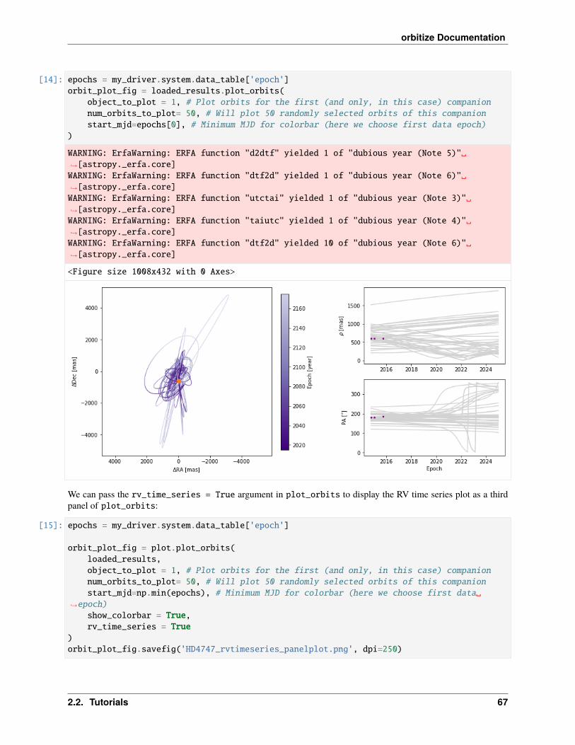
orbitize Documentation
[14]: epochs = my_driver.system.data_table['epoch']orbit_plot_fig = loaded_results.plot_orbits(
object_to_plot = 1, # Plot orbits for the first (and only, in this case) companionnum_orbits_to_plot= 50, # Will plot 50 randomly selected orbits of this companionstart_mjd=epochs[0], # Minimum MJD for colorbar (here we choose first data epoch)
)
WARNING: ErfaWarning: ERFA function "d2dtf" yielded 1 of "dubious year (Note 5)"→˓[astropy._erfa.core]WARNING: ErfaWarning: ERFA function "dtf2d" yielded 1 of "dubious year (Note 6)"→˓[astropy._erfa.core]WARNING: ErfaWarning: ERFA function "utctai" yielded 1 of "dubious year (Note 3)"→˓[astropy._erfa.core]WARNING: ErfaWarning: ERFA function "taiutc" yielded 1 of "dubious year (Note 4)"→˓[astropy._erfa.core]WARNING: ErfaWarning: ERFA function "dtf2d" yielded 10 of "dubious year (Note 6)"→˓[astropy._erfa.core]
<Figure size 1008x432 with 0 Axes>
We can pass the rv_time_series = True argument in plot_orbits to display the RV time series plot as a thirdpanel of plot_orbits:
[15]: epochs = my_driver.system.data_table['epoch']
orbit_plot_fig = plot.plot_orbits(loaded_results,object_to_plot = 1, # Plot orbits for the first (and only, in this case) companionnum_orbits_to_plot= 50, # Will plot 50 randomly selected orbits of this companionstart_mjd=np.min(epochs), # Minimum MJD for colorbar (here we choose first data
→˓epoch)show_colorbar = True,rv_time_series = True
)orbit_plot_fig.savefig('HD4747_rvtimeseries_panelplot.png', dpi=250)
2.2. Tutorials 67
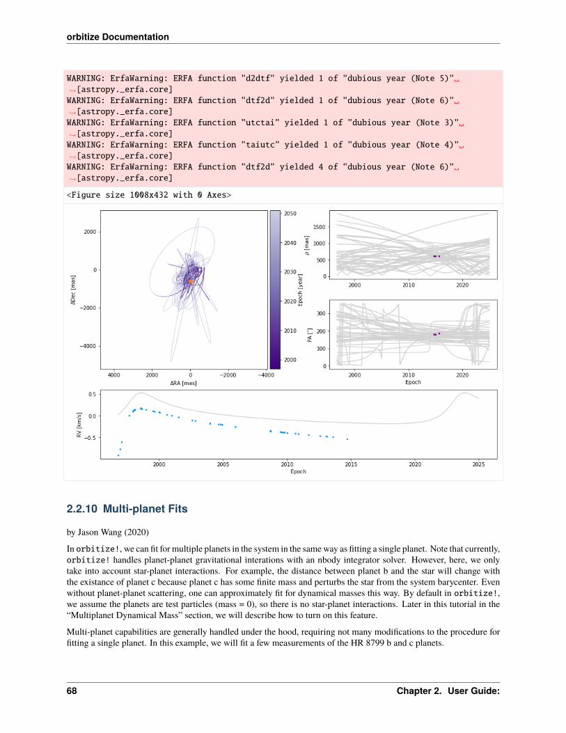
orbitize Documentation
WARNING: ErfaWarning: ERFA function "d2dtf" yielded 1 of "dubious year (Note 5)"→˓[astropy._erfa.core]WARNING: ErfaWarning: ERFA function "dtf2d" yielded 1 of "dubious year (Note 6)"→˓[astropy._erfa.core]WARNING: ErfaWarning: ERFA function "utctai" yielded 1 of "dubious year (Note 3)"→˓[astropy._erfa.core]WARNING: ErfaWarning: ERFA function "taiutc" yielded 1 of "dubious year (Note 4)"→˓[astropy._erfa.core]WARNING: ErfaWarning: ERFA function "dtf2d" yielded 4 of "dubious year (Note 6)"→˓[astropy._erfa.core]
<Figure size 1008x432 with 0 Axes>
2.2.10 Multi-planet Fits
by Jason Wang (2020)
In orbitize!, we can fit for multiple planets in the system in the same way as fitting a single planet. Note that currently,orbitize! handles planet-planet gravitational interations with an nbody integrator solver. However, here, we onlytake into account star-planet interactions. For example, the distance between planet b and the star will change withthe existance of planet c because planet c has some finite mass and perturbs the star from the system barycenter. Evenwithout planet-planet scattering, one can approximately fit for dynamical masses this way. By default in orbitize!,we assume the planets are test particles (mass = 0), so there is no star-planet interactions. Later in this tutorial in the“Multiplanet Dynamical Mass” section, we will describe how to turn on this feature.
Multi-planet capabilities are generally handled under the hood, requiring not many modifications to the procedure forfitting a single planet. In this example, we will fit a few measurements of the HR 8799 b and c planets.
68 Chapter 2. User Guide:

orbitize Documentation
[1]: import osimport orbitizeimport orbitize.driver
In this tutorial, we will do an example with OFTI just because it is fast. However, in most cases, you will likely wantto use MCMC as OFTI slows down significantly with multiple planets (even if each planet only has two astrometricdata points as shown in the example). MCMC also requires longer run time typically, but it generally scales better thanOFTI.
We follow the same steps as in the OFTI tutorial but set number of secondary bodies to 2 and read in a data filethat contains astrometry for two planets in the system (in the example, a shortened version of the HR 8799 b and castrometry). For MCMC, do the same thing as the single planet MCMC tutorial and make the same challenges as wehave here with OFTI. In summary, all that needs to be done is to include both planets’ measurements in the input datafile and adjust the number of secondary bodies in the system.
[2]: input_file = os.path.join(orbitize.DATADIR, "test_val_multi.csv")my_driver = orbitize.driver.Driver(input_file, 'OFTI',
2, # number of secondary bodies in system1.52, # total mass [M_sun]24.76, # total parallax of system [mas]mass_err=0.15,plx_err=0.64)
Converting ra/dec data points in data_table to sep/pa. Original data are stored in input_→˓table.
Next we run the sampler as usual:
[3]: s = my_driver.samplerorbits = s.run_sampler(1000)
With two planets, we have 2 sets of 6 orbtial parameters as well as the 2 system parameters (parallax and total mass).Our posterior, stored in orbits, is a (1000 x 14) array instead of the (1000 x 8) array had we fit a single planet.
As it gets confusing to track with index corresponds to which orbital parameter, we recommend you use the sys-tem.param_idx to index the parameters you are interested in. As a reminder, the abbreviations are: semi-major axis(sma), eccentricity (ecc), inclination (inc), argument of periastron (aop), position angle of nodes (pan), and epoch ofperiastron passage in fraction of the orbital period (tau). The 1 and 2 correspond to the two secondary bodies (in thiscase, HR 8799 b and HR 8799 c respectively)
[4]: print(orbits[0])print(orbits.shape)print(s.system.param_idx)
[56.24156344 0.27898557 0.30103121 1.9027183 2.28889823 0.4642520666.25721525 0.58545346 1.68028001 4.79289978 2.23970056 0.3390115524.8454356 1.43000678](1000, 14)'sma1': 0, 'ecc1': 1, 'inc1': 2, 'aop1': 3, 'pan1': 4, 'tau1': 5, 'sma2': 6, 'ecc2': 7,→˓'inc2': 8, 'aop2': 9, 'pan2': 10, 'tau2': 11, 'plx': 12, 'mtot': 13
2.2. Tutorials 69
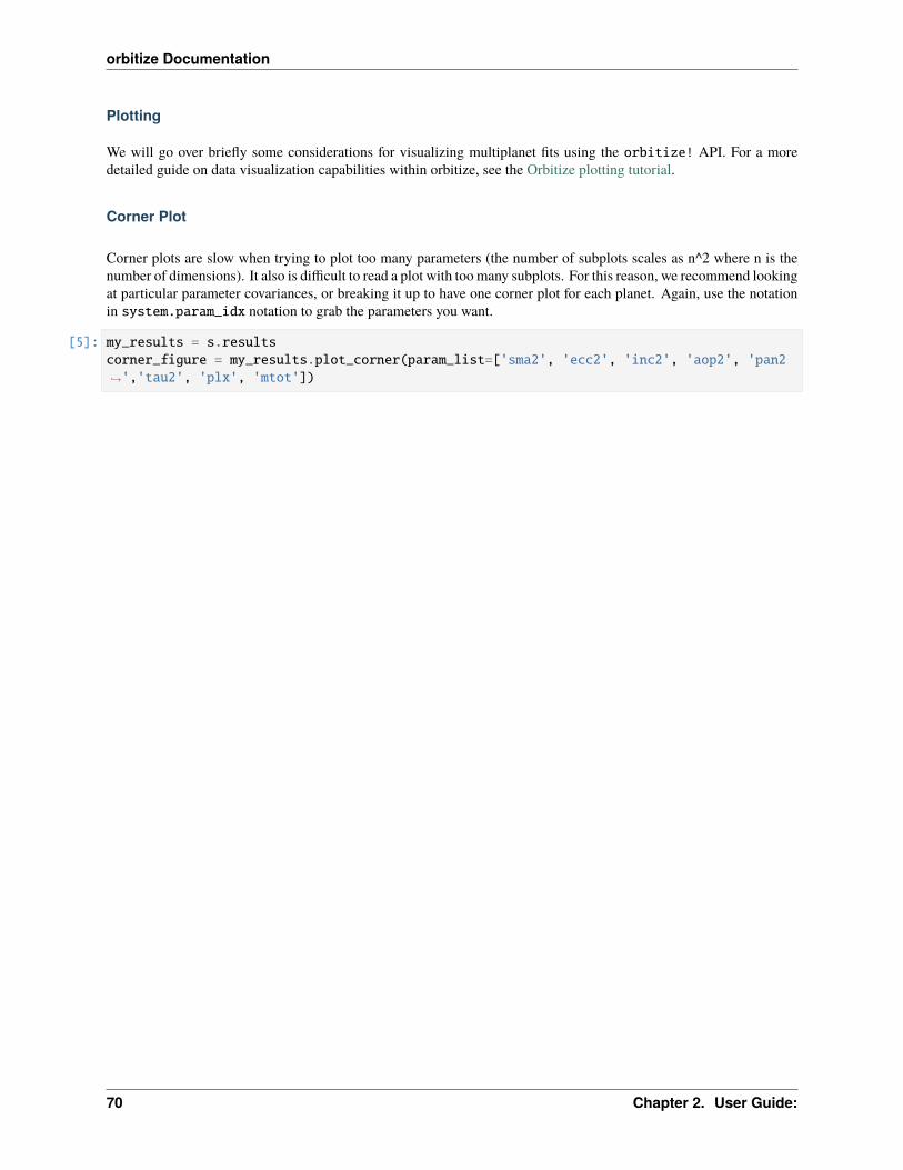
orbitize Documentation
Plotting
We will go over briefly some considerations for visualizing multiplanet fits using the orbitize! API. For a moredetailed guide on data visualization capabilities within orbitize, see the Orbitize plotting tutorial.
Corner Plot
Corner plots are slow when trying to plot too many parameters (the number of subplots scales as n^2 where n is thenumber of dimensions). It also is difficult to read a plot with too many subplots. For this reason, we recommend lookingat particular parameter covariances, or breaking it up to have one corner plot for each planet. Again, use the notationin system.param_idx notation to grab the parameters you want.
[5]: my_results = s.resultscorner_figure = my_results.plot_corner(param_list=['sma2', 'ecc2', 'inc2', 'aop2', 'pan2→˓','tau2', 'plx', 'mtot'])
70 Chapter 2. User Guide:

orbitize Documentation
Orbit Plot
Currently, the orbit plotting tool in results class only plots the orbit of one body at a time. You can select which bodyyou wish to plot.
[6]: epochs = my_driver.system.data_table['epoch']
orbit_figure = my_results.plot_orbits(start_mjd=epochs[0], # Minimum MJD for colorbar (here we choose first data epoch),object_to_plot=2 # plot planet c
)
2.2. Tutorials 71
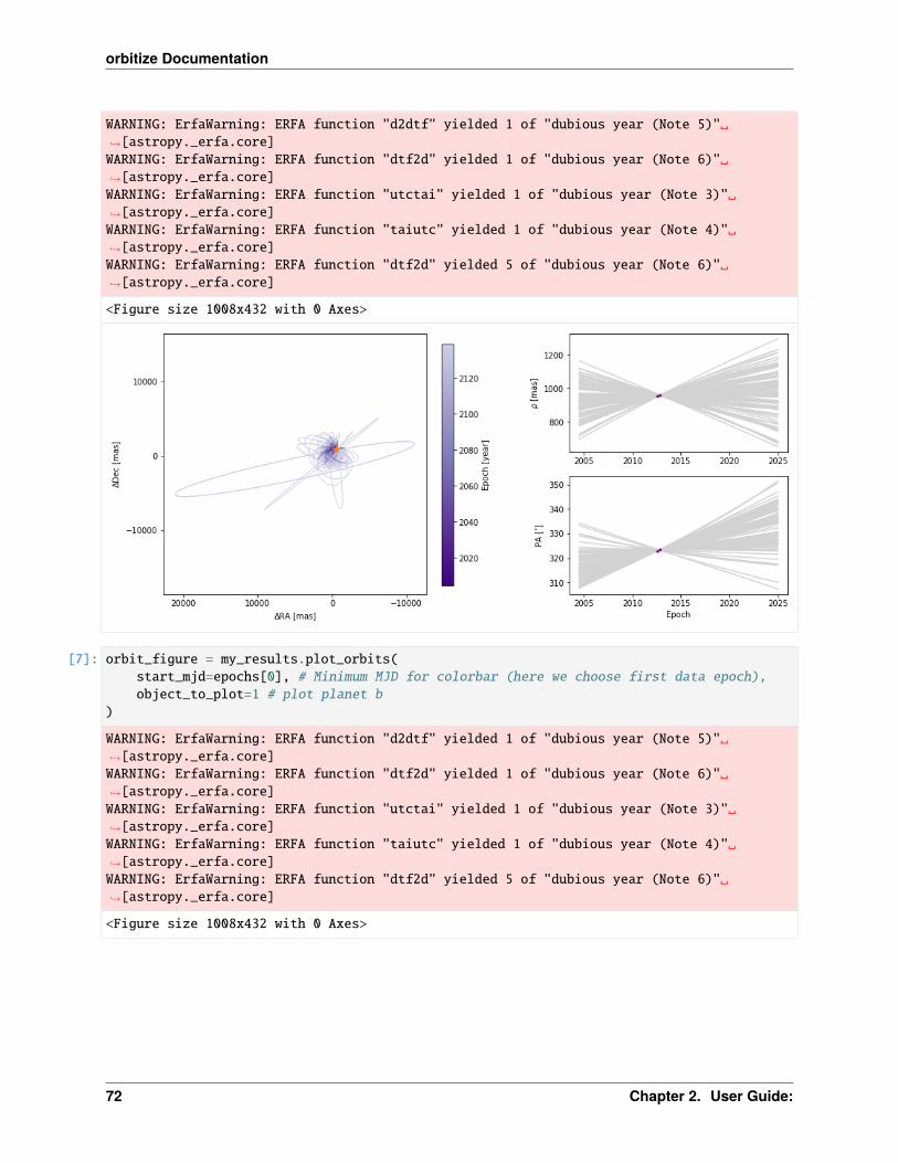
orbitize Documentation
WARNING: ErfaWarning: ERFA function "d2dtf" yielded 1 of "dubious year (Note 5)"→˓[astropy._erfa.core]WARNING: ErfaWarning: ERFA function "dtf2d" yielded 1 of "dubious year (Note 6)"→˓[astropy._erfa.core]WARNING: ErfaWarning: ERFA function "utctai" yielded 1 of "dubious year (Note 3)"→˓[astropy._erfa.core]WARNING: ErfaWarning: ERFA function "taiutc" yielded 1 of "dubious year (Note 4)"→˓[astropy._erfa.core]WARNING: ErfaWarning: ERFA function "dtf2d" yielded 5 of "dubious year (Note 6)"→˓[astropy._erfa.core]
<Figure size 1008x432 with 0 Axes>
[7]: orbit_figure = my_results.plot_orbits(start_mjd=epochs[0], # Minimum MJD for colorbar (here we choose first data epoch),object_to_plot=1 # plot planet b
)
WARNING: ErfaWarning: ERFA function "d2dtf" yielded 1 of "dubious year (Note 5)"→˓[astropy._erfa.core]WARNING: ErfaWarning: ERFA function "dtf2d" yielded 1 of "dubious year (Note 6)"→˓[astropy._erfa.core]WARNING: ErfaWarning: ERFA function "utctai" yielded 1 of "dubious year (Note 3)"→˓[astropy._erfa.core]WARNING: ErfaWarning: ERFA function "taiutc" yielded 1 of "dubious year (Note 4)"→˓[astropy._erfa.core]WARNING: ErfaWarning: ERFA function "dtf2d" yielded 5 of "dubious year (Note 6)"→˓[astropy._erfa.core]
<Figure size 1008x432 with 0 Axes>
72 Chapter 2. User Guide:

orbitize Documentation
Multiplanet Dynamical Mass
In the case we want to fit dynamical masses, the procedure again remains unchanged as for a single planet system (asdescribed in the RV MCMC Tutorial). The only thing to be aware of the extra parameters for the indiviudal masses ofthe components. Again, use the system.param_idx dictionary to keep track of the indices instead of trying to keeptrack of the ordering in one’s head. Here, we will not demo a fit, but just show the increasing of parameters by 2 whenfitting for the masses of the two secondary bodies.
Here, the new parameters are m1 and m2, the masses of planets b and c. m0 remains the mass of the star.
[8]: input_file = os.path.join(orbitize.DATADIR, "test_val_multi.csv")my_driver = orbitize.driver.Driver(input_file, 'MCMC',
2, # number of secondary bodies in system1.52, # stellar mass [M_sun]24.76, # total parallax of system [mas]mass_err=0.15,plx_err=0.64,system_kwargs='fit_secondary_mass' : True )
print(my_driver.system.param_idx)print(len(my_driver.system.sys_priors))
'sma1': 0, 'ecc1': 1, 'inc1': 2, 'aop1': 3, 'pan1': 4, 'tau1': 5, 'sma2': 6, 'ecc2': 7,→˓'inc2': 8, 'aop2': 9, 'pan2': 10, 'tau2': 11, 'plx': 12, 'm1': 13, 'm2': 14, 'm0': 1516
2.2. Tutorials 73
orbitize Documentation
2.2.11 Using non-orbitize! Posteriors as Priors
By Jorge Llop-Sayson (2021)
This tutorial shows how to use posterior distribution from any source as orbitize! priors using a Kernel DensityEstimator (KDE).
The user will need their posterior chains, consisiting of any number of correlated parameters, which will be used to geta KDE fit of the chains to be used as priors to orbitize!.
Once the priors are initialized the user can select their favorite fit method.
Read Data
[1]: import sysimport numpy as npimport matplotlib.pyplot as pltimport orbitizefrom orbitize import system, priors, basis, read_input, DATADIRimport pandas as pdimport radvel.utils as rv_utimport radvel.orbit as rv_or
# Read RadVel posterior chainpdf_fromRadVel = pd.read_csv("/sample_radvel_chains.csv.bz2".format(DATADIR),→˓compression='bz2', index_col=0)
per1 = pdf_fromRadVel.per1 # Periodk1 = pdf_fromRadVel.k1 # Doppler semi-amplitudesecosw1 = pdf_fromRadVel.secosw1sesinw1 = pdf_fromRadVel.sesinw1tc1 = pdf_fromRadVel.tc1 # time of conj.
len_pdf = len(pdf_fromRadVel)
The quant_type column displays the type of data each row contains: astrometry (radec or seppa), or radial velocity(rv). For astrometry, quant1 column contains right ascension or separation, and the quant2 column contains declina-tion or position angle. For rv data, quant1 contains radial velocity data in km/s, while quant2 is filled with nan topreserve the data structure. The table contains each respective error column.
We can now initialize the Driver class. MCMC samplers take time to converge to absolute maxima in parameterspace, and the more parameters we introduce, the longer we expect it to take.
Format Data
In this example we use data from RadVel, so we want to change format to use it in orbitize.
[2]: # From P to sma:system_mass = 1 # [Msol]system_mass_err = 0.01 # [Msol]pdf_msys = np.random.normal(system_mass, system_mass_err, size=len_pdf)sma_prior = rv_ut.semi_major_axis(per1, pdf_msys)
# ecc from RadVel parametrization(continues on next page)
74 Chapter 2. User Guide:
orbitize Documentation
(continued from previous page)
ecc_prior = sesinw1**2 + secosw1**2
# little omega, i.e. argument of the periastron, from RadVel parametrizationw_prior = np.arctan2(sesinw1, secosw1) + np.pi #+pi bc of RadVelvs Orbitize conventionw_prior[w_prior>=np.pi] = w_prior[w_prior>=np.pi]-2*np.pi
# tau, i.e. fraction of elapsed time of node passage, from RadVel parametrizationtp1 = rv_or.timetrans_to_timeperi(tc1, per1, ecc_prior, w_prior)tau_prior = basis.tp_to_tau(tp1, 55000, per1)
# m1 priorm1sini_prior = rv_ut.Msini(k1, per1, pdf_msys, ecc_prior, Msini_units='jupiter') * 1e-3sini_prior = priors.SinPrior()i_prior_samples = sini_prior.draw_samples(len_pdf)m1_prior = m1sini_prior/np.sin(i_prior_samples)
We now have the orbital parameters that are accessible with RV: SMA, eccentricity, argument of periastron, and tau.Plus, given that we obtained Msini from RV, we draw random values for the inclination to get correlated values for m1and inc. We thus end in this case with a correlated 6-parameter set.
Initialize Priors
We initilize the System object to initialize the priors
[3]: # Initialize System object which stores data & sets priorsdata_table = read_input.read_file("/test_val.csv".format(DATADIR)) #read datanum_secondary_bodies = 1
system_orbitize = system.System(num_secondary_bodies, data_table, system_mass,1e1, mass_err=system_mass_err, plx_err=0.1, tau_ref_epoch=55000,fit_secondary_
→˓mass=True,)
param_idx = system_orbitize.param_idx
print(param_idx)
'sma1': 0, 'ecc1': 1, 'inc1': 2, 'aop1': 3, 'pan1': 4, 'tau1': 5, 'plx': 6, 'gamma_defrv→˓': 7, 'sigma_defrv': 8, 'm1': 9, 'm0': 10
Let’s initilize the KDE prior object with the default bandwidth.
[4]: from scipy.stats import gaussian_kde
# The values go into a matrixtotal_params = 6values = np.empty((total_params,len_pdf))values[0,:] = sma_priorvalues[1,:] = ecc_priorvalues[2,:] = i_prior_samples
(continues on next page)
2.2. Tutorials 75

orbitize Documentation
(continued from previous page)
values[3,:] = w_priorvalues[4,:] = tau_priorvalues[5,:] = m1_prior
kde = gaussian_kde(values, bw_method=None) # None indicates that the KDE bandwidth is→˓set to defaultkde_prior_obj = priors.KDEPrior(kde, total_params)#,bounds=bounds_priors,log_scale_→˓arr=[False,False,False,False,False,False])
system_orbitize.sys_priors[param_idx['sma1']] = kde_prior_obj#priors.GaussianPrior(np.→˓mean(sma_prior), np.std(sma_prior))#priors.KDEPrior(gaussian_kde(values[0,:], bw_→˓method=None),1)#kde_prior_obj#system_orbitize.sys_priors[param_idx['ecc1']] = kde_prior_obj#priors.GaussianPrior(np.→˓mean(ecc_prior), np.std(ecc_prior))#kde_prior_obj#priors.GaussianPrior(np.mean(pdf_→˓fromRadVel['e1']), np.std(pdf_fromRadVel['e1']))#priors.KDEPrior(gaussian_kde(values[1,:],→˓ bw_method=None),1)#kde_prior_objsystem_orbitize.sys_priors[param_idx['inc1']] = kde_prior_objsystem_orbitize.sys_priors[param_idx['aop1']] = kde_prior_obj#priors.GaussianPrior(np.→˓mean(w_prior), 0.1)#kde_prior_obj#kde_prior_objsystem_orbitize.sys_priors[param_idx['tau1']] = kde_prior_obj#priors.GaussianPrior(np.→˓mean(tau_prior), 0.01)#np.std(tau_prior))#kde_prior_obj#kde_prior_obj#priors.→˓KDEPrior(gaussian_kde(values[4,:], bw_method=None),1)#kde_prior_objsystem_orbitize.sys_priors[-2] = kde_prior_obj
We can plot the KDE fit against the actual distribution to see if the selected bandwidth is adecuate for the data.
[5]: fig, axs = plt.subplots(2, 3,figsize=(11,6))# smaaxs[0, 0].hist(kde.resample(len_pdf)[0,:],100,density=True,color='b',label='Posterior→˓Draw',stacked=True)axs[0, 0].hist(sma_prior,100,density=True,color='r',histtype = 'step',label='Prior Draw',→˓stacked=True)#color='r')#axs[0, 0].set_xlabel('SMA [AU]')axs[0, 0].set_yticklabels([])# eccaxs[0, 1].hist(kde.resample(len_pdf)[1,:],100,density=True,color='b',label='Posterior→˓Draw',stacked=True)axs[0, 1].hist(ecc_prior,100,density=True,color='r',histtype = 'step',label='Prior Draw',→˓stacked=True)#color='r')#axs[0, 1].set_xlabel('eccentricity')axs[0, 1].set_yticklabels([])# massmasskde_arr = kde.resample(len_pdf)[-1,:]masskde_arr = masskde_arr[masskde_arr<0.003]m1_prior_draw = m1_prior[m1_prior<0.003]axs[1,0].hist(masskde_arr,100,density=True,color='b',label='Posterior Draw',stacked=True)axs[1,0].hist((m1_prior_draw),100,density=True,color='r',histtype = 'step',label='Prior→˓Draw',stacked=True)#color='r')#axs[1, 0].set_xlabel('$Mass_b$ [$M_Jup$]')axs[1, 0].set_yticklabels([])# incaxs[1,1].hist(np.rad2deg(kde.resample(len_pdf)[2,:]),100,density=True,color='b',label=→˓'Posterior Draw',stacked=True) (continues on next page)
76 Chapter 2. User Guide:
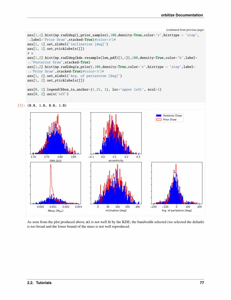
orbitize Documentation
(continued from previous page)
axs[1,1].hist(np.rad2deg(i_prior_samples),100,density=True,color='r',histtype = 'step',→˓label='Prior Draw',stacked=True)#color='r')#axs[1, 1].set_xlabel('inclination [deg]')axs[1, 1].set_yticklabels([])# waxs[1,2].hist(np.rad2deg(kde.resample(len_pdf)[3,:]),100,density=True,color='b',label=→˓'Posterior Draw',stacked=True)axs[1,2].hist(np.rad2deg(w_prior),100,density=True,color='r',histtype = 'step',label=→˓'Prior Draw',stacked=True)#color='r')#axs[1, 2].set_xlabel('Arg. of periastron [deg]')axs[1, 2].set_yticklabels([])
axs[0, 1].legend(bbox_to_anchor=(1.25, 1), loc='upper left', ncol=1)axs[0, 2].axis('off')
[5]: (0.0, 1.0, 0.0, 1.0)
As seen from the plot produced above, m1 is not well fit by the KDE; the bandwidth selected (we selected the default)is too broad and the lower bound of the mass is not well reproduced.
2.2. Tutorials 77
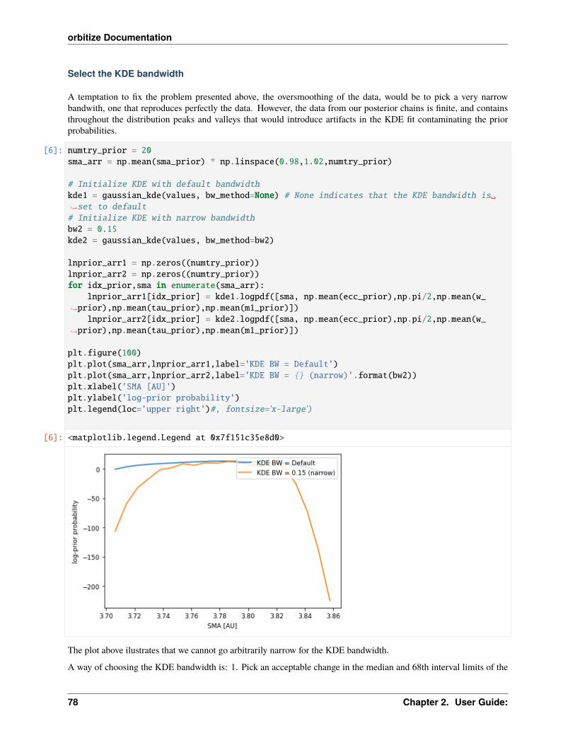
orbitize Documentation
Select the KDE bandwidth
A temptation to fix the problem presented above, the oversmoothing of the data, would be to pick a very narrowbandwith, one that reproduces perfectly the data. However, the data from our posterior chains is finite, and containsthroughout the distribution peaks and valleys that would introduce artifacts in the KDE fit contaminating the priorprobabilities.
[6]: numtry_prior = 20sma_arr = np.mean(sma_prior) * np.linspace(0.98,1.02,numtry_prior)
# Initialize KDE with default bandwidthkde1 = gaussian_kde(values, bw_method=None) # None indicates that the KDE bandwidth is→˓set to default# Initialize KDE with narrow bandwidthbw2 = 0.15kde2 = gaussian_kde(values, bw_method=bw2)
lnprior_arr1 = np.zeros((numtry_prior))lnprior_arr2 = np.zeros((numtry_prior))for idx_prior,sma in enumerate(sma_arr):
lnprior_arr1[idx_prior] = kde1.logpdf([sma, np.mean(ecc_prior),np.pi/2,np.mean(w_→˓prior),np.mean(tau_prior),np.mean(m1_prior)])
lnprior_arr2[idx_prior] = kde2.logpdf([sma, np.mean(ecc_prior),np.pi/2,np.mean(w_→˓prior),np.mean(tau_prior),np.mean(m1_prior)])
plt.figure(100)plt.plot(sma_arr,lnprior_arr1,label='KDE BW = Default')plt.plot(sma_arr,lnprior_arr2,label='KDE BW = (narrow)'.format(bw2))plt.xlabel('SMA [AU]')plt.ylabel('log-prior probability')plt.legend(loc='upper right')#, fontsize='x-large')
[6]: <matplotlib.legend.Legend at 0x7f151c35e8d0>
The plot above ilustrates that we cannot go arbitrarily narrow for the KDE bandwidth.
A way of choosing the KDE bandwidth is: 1. Pick an acceptable change in the median and 68th interval limits of the
78 Chapter 2. User Guide:
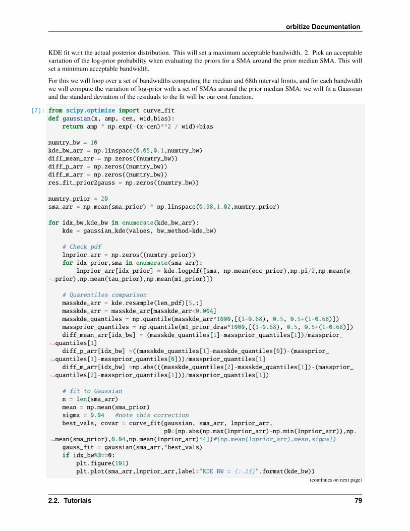
orbitize Documentation
KDE fit w.r.t the actual posterior distribution. This will set a maximum acceptable bandwidth. 2. Pick an acceptablevariation of the log-prior probability when evaluating the priors for a SMA around the prior median SMA. This willset a minimum acceptable bandwidth.
For this we will loop over a set of bandwidths computing the median and 68th interval limits, and for each bandwidthwe will compute the variation of log-prior with a set of SMAs around the prior median SMA: we will fit a Gaussianand the standard deviation of the residuals to the fit will be our cost function.
[7]: from scipy.optimize import curve_fitdef gaussian(x, amp, cen, wid,bias):
return amp * np.exp(-(x-cen)**2 / wid)+bias
numtry_bw = 10kde_bw_arr = np.linspace(0.05,0.1,numtry_bw)diff_mean_arr = np.zeros((numtry_bw))diff_p_arr = np.zeros((numtry_bw))diff_m_arr = np.zeros((numtry_bw))res_fit_prior2gauss = np.zeros((numtry_bw))
numtry_prior = 20sma_arr = np.mean(sma_prior) * np.linspace(0.98,1.02,numtry_prior)
for idx_bw,kde_bw in enumerate(kde_bw_arr):kde = gaussian_kde(values, bw_method=kde_bw)
# Check pdflnprior_arr = np.zeros((numtry_prior))for idx_prior,sma in enumerate(sma_arr):
lnprior_arr[idx_prior] = kde.logpdf([sma, np.mean(ecc_prior),np.pi/2,np.mean(w_→˓prior),np.mean(tau_prior),np.mean(m1_prior)])
# Quarentiles comparisonmasskde_arr = kde.resample(len_pdf)[5,:]masskde_arr = masskde_arr[masskde_arr<0.004]masskde_quantiles = np.quantile(masskde_arr*1000,[(1-0.68), 0.5, 0.5+(1-0.68)])massprior_quantiles = np.quantile(m1_prior_draw*1000,[(1-0.68), 0.5, 0.5+(1-0.68)])diff_mean_arr[idx_bw] = (masskde_quantiles[1]-massprior_quantiles[1])/massprior_
→˓quantiles[1]diff_p_arr[idx_bw] =((masskde_quantiles[1]-masskde_quantiles[0])-(massprior_
→˓quantiles[1]-massprior_quantiles[0]))/massprior_quantiles[1]diff_m_arr[idx_bw] =np.abs(((masskde_quantiles[2]-masskde_quantiles[1])-(massprior_
→˓quantiles[2]-massprior_quantiles[1]))/massprior_quantiles[1])
# fit to Gaussiann = len(sma_arr)mean = np.mean(sma_prior)sigma = 0.04 #note this correctionbest_vals, covar = curve_fit(gaussian, sma_arr, lnprior_arr,
p0=[np.abs(np.max(lnprior_arr)-np.min(lnprior_arr)),np.→˓mean(sma_prior),0.04,np.mean(lnprior_arr)*4])#[np.mean(lnprior_arr),mean,sigma])
gauss_fit = gaussian(sma_arr,*best_vals)if idx_bw%3==0:
plt.figure(101)plt.plot(sma_arr,lnprior_arr,label="KDE BW = :.2f".format(kde_bw))
(continues on next page)
2.2. Tutorials 79
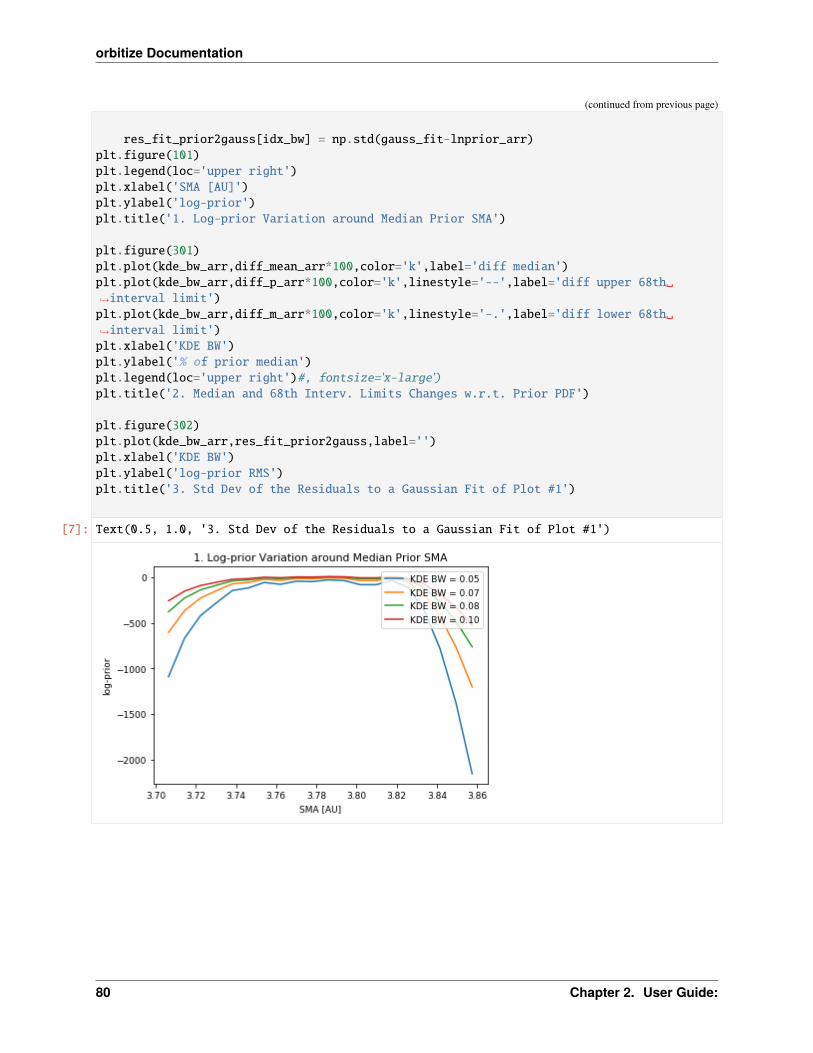
orbitize Documentation
(continued from previous page)
res_fit_prior2gauss[idx_bw] = np.std(gauss_fit-lnprior_arr)plt.figure(101)plt.legend(loc='upper right')plt.xlabel('SMA [AU]')plt.ylabel('log-prior')plt.title('1. Log-prior Variation around Median Prior SMA')
plt.figure(301)plt.plot(kde_bw_arr,diff_mean_arr*100,color='k',label='diff median')plt.plot(kde_bw_arr,diff_p_arr*100,color='k',linestyle='--',label='diff upper 68th→˓interval limit')plt.plot(kde_bw_arr,diff_m_arr*100,color='k',linestyle='-.',label='diff lower 68th→˓interval limit')plt.xlabel('KDE BW')plt.ylabel('% of prior median')plt.legend(loc='upper right')#, fontsize='x-large')plt.title('2. Median and 68th Interv. Limits Changes w.r.t. Prior PDF')
plt.figure(302)plt.plot(kde_bw_arr,res_fit_prior2gauss,label='')plt.xlabel('KDE BW')plt.ylabel('log-prior RMS')plt.title('3. Std Dev of the Residuals to a Gaussian Fit of Plot #1')
[7]: Text(0.5, 1.0, '3. Std Dev of the Residuals to a Gaussian Fit of Plot #1')
80 Chapter 2. User Guide:
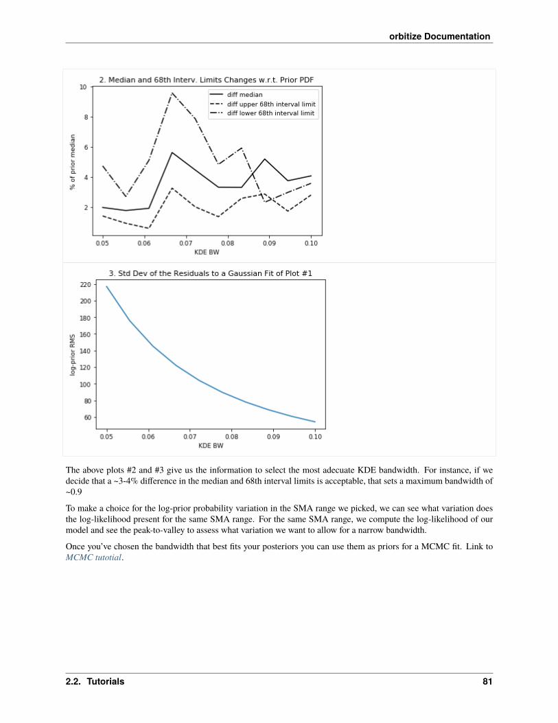
orbitize Documentation
The above plots #2 and #3 give us the information to select the most adecuate KDE bandwidth. For instance, if wedecide that a ~3-4% difference in the median and 68th interval limits is acceptable, that sets a maximum bandwidth of~0.9
To make a choice for the log-prior probability variation in the SMA range we picked, we can see what variation doesthe log-likelihood present for the same SMA range. For the same SMA range, we compute the log-likelihood of ourmodel and see the peak-to-valley to assess what variation we want to allow for a narrow bandwidth.
Once you’ve chosen the bandwidth that best fits your posteriors you can use them as priors for a MCMC fit. Link toMCMC tutotial.
2.2. Tutorials 81

orbitize Documentation
2.2.12 Fitting in different orbital bases
In this tutorial, we show how one can perform orbit-fits in different coordinate bases amongst the ones supported byorbitize. Currently fitting in different bases is only supported in MCMC, so we will use MCMC to perform anorbit-fit in an orbital basis distinct from the default one. For a general introduction to MCMC, be sure to check out theMCMC Introduction tutorial first!
The “standard” and “XYZ” bases
The default way to define an orbit in orbitize is through what we call the ‘standard basis’, which consists of eightparameters: semi-major axis (sma), eccentricity (ecc), inclination (inc), argument of periastron (aop), position angleof the nodes (pan), epoch of periastron expressed as a fraction of the period past a reference epoch (tau), parallax (plx)and total system mass (mtot). Each orbital element has an associated default prior; to see how to explore and modifythese priors check out the Modifying priors tutorial.
An alternative way to define an orbit is through its position and velocity components in XYZ space for a given epoch;we will call this the ‘XYZ basis’. The orbit is thus defined with the array (𝑥, 𝑦, 𝑧, , ,, plx, mtot), with positioncoordinates measured in AU and velocity components in km s−1. In this basis, the sky-plane coordinates (𝑥, 𝑦) are theseparations of the planet relative to the primary, with the positive 𝑥 and 𝑦 directions coinciding with the positive RAand Dec directions, respectively. The 𝑧 direction is the line-of-sight coordinate, such that movement in the positive 𝑧direction causes a redshift. The default priors are uniform all uniform.
Setting up Sampler in the XYZ basis
The easiest way to run an orbit-fit in an alternative orbital basis in orbitize is through the orbitize.driver.Driverinterface. The process is exactly like initializing a regular Driver object, but setting the fitting_basis keyword to‘XYZ’:
[1]: import numpy as np
import orbitizefrom orbitize import driverimport multiprocessing as mp
filename = "xyz_test_data.csv".format(orbitize.DATADIR) # a file with input in radec→˓since rn it only works for that
# system parametersnum_secondary_bodies = 1system_mass = 1.75 # [Msol]plx = 51.44 # [mas]mass_err = 0.05 # [Msol]plx_err = 0.12 # [mas]
# MCMC parametersnum_temps = 5num_walkers = 20num_threads = mp.cpu_count() # or a different number if you prefer
my_driver = driver.Driver(filename, 'MCMC', num_secondary_bodies, system_mass, plx, mass_err=mass_err, plx_
→˓err=plx_err,(continues on next page)
82 Chapter 2. User Guide:

orbitize Documentation
(continued from previous page)
mcmc_kwargs='num_temps': num_temps, 'num_walkers': num_walkers, 'num_threads': num_→˓threads,
system_kwargs='fitting_basis': 'XYZ')
s = my_driver.sampler
Converting ra/dec data points in data_table to sep/pa. Original data are stored in input_→˓table.
(Properly) initializing walkers in the XYZ basis
In the standard basis at this point we would be ready to use the s.run_sampler method to start the sampling, but withthe XYZ basis we have to make sure that all our walkers are initialized in a valid region of parameter space. This isbecause randomly generated values of (𝑥, 𝑦, 𝑧, , , ) can result in unbound, invalid orbits with, for example, negativeeccentricities (which is not cool). This can be easily corrected with the s.validate_xyz_positions method:
[2]: s.validate_xyz_positions()
All walker positions validated.
/home/sblunt/Projects/orbitize/orbitize/basis.py:944: RuntimeWarning: invalid value→˓encountered in arccoseanom = np.arccos(cos_eanom)
/data/user/sblunt/miniconda3/envs/python3.7/lib/python3.7/site-packages/astropy/units/→˓quantity.py:481: RuntimeWarning: invalid value encountered in sqrtresult = super().__array_ufunc__(function, method, *arrays, **kwargs)
After this is done, the sampler can be run and the results saved normally:
[3]: total_orbits = 600 # number of steps x number of walkers (at lowest temperature)burn_steps = 10 # steps to burn in per walkerthin = 2 # only save every 2nd step
s.run_sampler(total_orbits, burn_steps=burn_steps, thin=thin)s.results.save_results('my_posterior.hdf5')
/data/user/sblunt/miniconda3/envs/python3.7/lib/python3.7/site-packages/astropy/table/→˓column.py:1020: RuntimeWarning: invalid value encountered in greaterresult = getattr(super(), op)(other)
/home/sblunt/Projects/orbitize/orbitize/kepler.py:112: RuntimeWarning: invalid value→˓encountered in sqrttanom = 2.*np.arctan(np.sqrt((1.0 + ecc)/(1.0 - ecc))*np.tan(0.5*eanom))
Starting Burn in
/data/user/sblunt/miniconda3/envs/python3.7/lib/python3.7/site-packages/astropy/table/→˓column.py:1020: RuntimeWarning: invalid value encountered in greaterresult = getattr(super(), op)(other)
/home/sblunt/Projects/orbitize/orbitize/kepler.py:112: RuntimeWarning: invalid value→˓encountered in sqrttanom = 2.*np.arctan(np.sqrt((1.0 + ecc)/(1.0 - ecc))*np.tan(0.5*eanom))
(continues on next page)
2.2. Tutorials 83
orbitize Documentation
(continued from previous page)
/data/user/sblunt/miniconda3/envs/python3.7/lib/python3.7/site-packages/astropy/table/→˓column.py:1020: RuntimeWarning: invalid value encountered in greaterresult = getattr(super(), op)(other)
/home/sblunt/Projects/orbitize/orbitize/kepler.py:112: RuntimeWarning: invalid value→˓encountered in sqrttanom = 2.*np.arctan(np.sqrt((1.0 + ecc)/(1.0 - ecc))*np.tan(0.5*eanom))
10/10 steps of burn-in completeBurn in complete. Sampling posterior now.
84 Chapter 2. User Guide:

orbitize Documentation
/data/user/sblunt/miniconda3/envs/python3.7/lib/python3.7/site-packages/astropy/table/→˓column.py:1020: RuntimeWarning: invalid value encountered in greaterresult = getattr(super(), op)(other)
/home/sblunt/Projects/orbitize/orbitize/kepler.py:112: RuntimeWarning: invalid value→˓encountered in sqrttanom = 2.*np.arctan(np.sqrt((1.0 + ecc)/(1.0 - ecc))*np.tan(0.5*eanom))
/data/user/sblunt/miniconda3/envs/python3.7/lib/python3.7/site-packages/astropy/table/→˓column.py:1020: RuntimeWarning: invalid value encountered in greaterresult = getattr(super(), op)(other)
/home/sblunt/Projects/orbitize/orbitize/kepler.py:112: RuntimeWarning: invalid value→˓encountered in sqrt
(continues on next page)
2.2. Tutorials 85
orbitize Documentation
(continued from previous page)
tanom = 2.*np.arctan(np.sqrt((1.0 + ecc)/(1.0 - ecc))*np.tan(0.5*eanom))
/data/user/sblunt/miniconda3/envs/python3.7/lib/python3.7/site-packages/astropy/table/→˓column.py:1020: RuntimeWarning: invalid value encountered in greaterresult = getattr(super(), op)(other)
/home/sblunt/Projects/orbitize/orbitize/kepler.py:112: RuntimeWarning: invalid value→˓encountered in sqrttanom = 2.*np.arctan(np.sqrt((1.0 + ecc)/(1.0 - ecc))*np.tan(0.5*eanom))
/data/user/sblunt/miniconda3/envs/python3.7/lib/python3.7/site-packages/astropy/table/→˓column.py:1020: RuntimeWarning: invalid value encountered in greaterresult = getattr(super(), op)(other)
/home/sblunt/Projects/orbitize/orbitize/kepler.py:112: RuntimeWarning: invalid value→˓encountered in sqrttanom = 2.*np.arctan(np.sqrt((1.0 + ecc)/(1.0 - ecc))*np.tan(0.5*eanom))
/data/user/sblunt/miniconda3/envs/python3.7/lib/python3.7/site-packages/astropy/table/→˓column.py:1020: RuntimeWarning: invalid value encountered in greater (continues on next page)
86 Chapter 2. User Guide:
orbitize Documentation
(continued from previous page)
result = getattr(super(), op)(other)/home/sblunt/Projects/orbitize/orbitize/kepler.py:112: RuntimeWarning: invalid value→˓encountered in sqrttanom = 2.*np.arctan(np.sqrt((1.0 + ecc)/(1.0 - ecc))*np.tan(0.5*eanom))
/data/user/sblunt/miniconda3/envs/python3.7/lib/python3.7/site-packages/astropy/table/→˓column.py:1020: RuntimeWarning: invalid value encountered in greaterresult = getattr(super(), op)(other)
/home/sblunt/Projects/orbitize/orbitize/kepler.py:112: RuntimeWarning: invalid value→˓encountered in sqrttanom = 2.*np.arctan(np.sqrt((1.0 + ecc)/(1.0 - ecc))*np.tan(0.5*eanom))
30/30 steps completedRun complete
Loading and converting results
You can load the results as you normally would. The orbit posteriors are saved in the results.post attribute, and thebasis you used for the fit in the results.fitting_basis attribute:
[4]: myResults = orbitize.results.Results() # create empty Results objectmyResults.load_results('my_posterior.hdf5')print('The used basis for the fit was ', myResults.fitting_basis)print('The posteriors are ', myResults.post)
Converting ra/dec data points in data_table to sep/pa. Original data are stored in input_→˓table.The used basis for the fit was XYZThe posteriors are [[-1.55895340e+01 -3.20352269e+01 9.38119986e+00 ... -7.46195838e-03
5.15299823e+01 1.72400897e+00][-1.56081092e+01 -3.20562773e+01 1.49810951e+00 ... 8.53387015e-025.13883909e+01 1.73579787e+00]
[-1.55612462e+01 -3.20801251e+01 -2.96308303e-01 ... 7.18261775e-015.14206555e+01 1.76608956e+00]
...[-1.55671475e+01 -3.20089823e+01 3.62094122e+01 ... 3.72598271e-015.15487665e+01 1.74432532e+00]
[-1.55794884e+01 -3.20303979e+01 2.75912018e+01 ... -2.40407388e-015.14895599e+01 1.78876637e+00]
[-1.55837449e+01 -3.20532712e+01 1.93382300e+01 ... -1.24185021e-015.14598433e+01 1.80483891e+00]]
Let’s convert back to the good old standard basis:
[5]: xyz_posterior = myResults.post
standard_posterior = myResults.system.basis.to_standard_basis(xyz_posterior)
print('My posterior in standard basis is ', standard_posterior)
My posterior in standard basis is [[ 7.89543529 6.92670011 4.84646336 ... 0.→˓36153132 -6.60018059
1.52254522][ 1.00000429 1.00000659 0.96238341 ... 1.00053929 1.00014326
(continues on next page)
2.2. Tutorials 87
orbitize Documentation
(continued from previous page)
0.9999977 ][ 1.43499876 1.22274162 0.79516331 ... 1.46937244 2.46248534
1.23409917]...[-15.56714749 -32.00898233 36.20941224 ... 0.37259827 51.54876654
1.74432532][-15.57948843 -32.03039793 27.59120179 ... -0.24040739 51.48955988
1.78876637][-15.58374489 -32.0532712 19.33822997 ... -0.12418502 51.45984325
1.80483891]]
And we’re done! Enjoy the XYZ basis.
2.2.13 Working with the Hipparcos Intermediate Astrometric Data (IAD)
Sarah Blunt (2021)
The Hipparcos IAD are notoriously annoying to work with, and several methods have been developed for incorporatingthem into orbit-fits. In this tutorial, we’ll take you through the method outlined in Nielsen et al. (2020). In the nearfuture, we’ll add in other algorithms (in particular, that of Brandt et al.).
The purpose of this tutorial is not to convince you that one method is better than the other, but rather to teach you touse the method of Nielsen et al. I recommend reading through Section 3.1 of Nielsen et al. (2020) before diving intothis tutorial.
If you want to skip right to “what’s the syntax for doing an orbit-fit with the IAD,” I suggest checking out the betaPictoris end-to-end test I coded up here.
This tutorial will take you through: - Obtaining the IAD for your object(s). - Refitting the IAD (i.e. re-doing the fit theHipparcos team did), which allows you to evaluate whether they are suitable for orbit-fitting. - Incorporating the IADinto your orbit-fit.
Part 1: Obtaining the IAD
orbitize! assumes the IAD are an updated version of the van Leeuwen (2007) re-reduction. You can learn about thedata here, and download them here. Note that this download will take ~350 MB of space; if you prefer to to keep thedata necessary for a few fits, you can download all the data and remove unnecessary files (or just send me an email).We’ve provided the IAD files for a few representative systems in this repository.
NOTE: if you prefer to use the DVD files, orbitize! can handle those as well. However, be warned that these filesdo not mark rejected scans.
The good news is that the hard part is actually getting the data. Once you have the file, orbitize! can read it in itsraw form.
88 Chapter 2. User Guide:

orbitize Documentation
Part 2: Refitting the IAD
Once you have the IAD, the next step is to convince yourself that they’re suitable for orbit-fitting (i.e. free of transcriptionerrors, etc). Here’s a handy function to do this (this should take a few mins to run, but if it’s taking much longer, youcan decrease the number of steps). This code reproduces the test at the end of Section 3.1 of Nielsen et al. (2020), socheck that out for more information.
[1]: import orbitizeimport osfrom datetime import datetime
from orbitize.hipparcos import nielsen_iad_refitting_test
# The Hipparcos ID of your target. Available on Simbad.hip_num = '027321'
# Name/path for the plot this function will makesaveplot = 'bPic_IADrefit.png'
# Location of the Hipparcos IAD file.IAD_file = 'H.d'.format(orbitize.DATADIR, hip_num)
# These `emcee` settings are sufficient for the 5-parameter fits we're about to run,# although I'd probably run it for 5,000-10,000 steps if I wanted to publish it.burn_steps = 100mcmc_steps = 500
start = datetime.now()
# run the fitprint('Go get a coffee. This will take a few mins! :)')nielsen_iad_refitting_test(
IAD_file,hip_num=hip_num,saveplot=saveplot,burn_steps=burn_steps,mcmc_steps=mcmc_steps
)
end = datetime.now()duration_mins = (end - start).total_seconds() / 60
print("Done! This fit took :.1f mins on my machine.".format(duration_mins))
# If you don't want to save the plot, you can run this line to remove it_ = os.system('rm '.format(saveplot))
Go get a coffee. This will take a few mins! :)Starting burn-in!Starting production chain!Done! This fit took 3.1 mins on my machine.
2.2. Tutorials 89
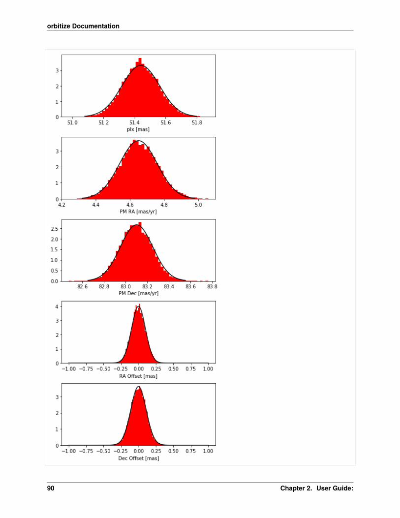
orbitize Documentation
90 Chapter 2. User Guide:
orbitize Documentation
Part 3: Using the IAD in your Orbit-fit
Congrats, you’ve now reproduced a Hipparcos fit! The last thing to do is actually run your orbit-fit. Here’s an example,also using the Gaia astrometric point from eDR3. This code snippet essentially repeats the beta Pictoris end-to-end testI coded up here.
[2]: import os.pathimport orbitizefrom orbitize import read_input, hipparcos, gaia, system, priors, sampler
"""As with most `orbitize!` fits, we'll start by reading in our data file. TheHipparcos data file is kept separate; your main data file only needs to containthe relative astrometry and RVs you're using in your fit."""
input_file = os.path.join(orbitize.DATADIR, 'betaPic.csv')data_table = read_input.read_file(input_file)
"""Next, we'll instantiate a `HipparcosLogProb` object."""num_secondary_bodies = 1 # number of planets/companions orbiting your primaryhipparcos_number='027321' # (can look up your object's Hipparcos ID on Simbad)hipparcos_filename=os.path.join(orbitize.DATADIR, 'H027321.d') # location of your IAD→˓data file
betaPic_Hip = hipparcos.HipparcosLogProb(hipparcos_filename, hipparcos_number, num_secondary_bodies
)
"""Next, instantiate a `GaiaLogProb` object."""betapic_edr3_number = 4792774797545800832betaPic_Gaia = gaia.GaiaLogProb(
betapic_edr3_number, betaPic_Hip, dr='edr3')
"""Next, we'll instantiate a `System` object, a container for all the informationrelevant to the system you're fitting."""
m0 = 1.75 # median mass of primary [M_sol]plx = 51.5 # [mas]fit_secondary_mass = True # Tell orbitize! we want to get dynamical masses
# (not possible with only relative astrometry).mass_err = 0.01 # we'll overwrite these in a secplx_err = 0.01
betaPic_system = system.System(num_secondary_bodies, data_table, m0, plx, hipparcos_IAD=betaPic_Hip,
(continues on next page)
2.2. Tutorials 91
orbitize Documentation
(continued from previous page)
gaia=betaPic_Gaia, fit_secondary_mass=fit_secondary_mass, mass_err=mass_err,plx_err=plx_err
)
"""If you'd like to change any priors from the defaults (given in Blunt et al. 2020),do it like this:"""
# set uniform parallax priorplx_index = betaPic_system.param_idx['plx']betaPic_system.sys_priors[plx_index] = priors.UniformPrior(plx - 1.0, plx + 1.0)
# set uniform primary mass priorm0_index = betaPic_system.param_idx['m0']betaPic_system.sys_priors[m0_index] = priors.UniformPrior(1.5, 2.0)
INFO: Query finished. [astroquery.utils.tap.core]
Finally, set up and run your MCMC!
[3]: """These are the MCMC parameters I'd use if I were publishing this fit.This would take a while to run (takes about a day on my machine)."""# num_threads = 50# num_temps = 20# num_walkers = 1000# num_steps = 10000000 # n_walkers x n_steps_per_walker# burn_steps = 10000# thin = 100
"""Here are some parameters you can use for the tutorial. These chains will notbe converged."""
num_threads = 1num_temps = 1num_walkers = 100num_steps = 10 # n_walkers x n_steps_per_walkerburn_steps = 10thin = 1
betaPic_sampler = sampler.MCMC(betaPic_system, num_threads=num_threads, num_temps=num_temps,num_walkers=num_walkers
)betaPic_sampler.run_sampler(num_steps, burn_steps=burn_steps, thin=thin)
Starting Burn in
/home/sblunt/Projects/orbitize/orbitize/priors.py:354: RuntimeWarning: invalid value→˓encountered in log
(continues on next page)
92 Chapter 2. User Guide:
orbitize Documentation
(continued from previous page)
lnprob = -np.log((element_array*normalizer))/home/sblunt/Projects/orbitize/orbitize/priors.py:463: RuntimeWarning: invalid value→˓encountered in loglnprob = np.log(np.sin(element_array)/normalization)
10/10 steps of burn-in completeBurn in complete. Sampling posterior now.
Run complete
[3]: <emcee.ensemble.EnsembleSampler at 0x7f2f2e3a2650>
[4]: # make corner plotfig = betaPic_sampler.results.plot_corner()
WARNING:root:Too few points to create valid contoursWARNING:root:Too few points to create valid contoursWARNING:root:Too few points to create valid contoursWARNING:root:Too few points to create valid contoursWARNING:root:Too few points to create valid contoursWARNING:root:Too few points to create valid contoursWARNING:root:Too few points to create valid contoursWARNING:root:Too few points to create valid contoursWARNING:root:Too few points to create valid contoursWARNING:root:Too few points to create valid contoursWARNING:root:Too few points to create valid contoursWARNING:root:Too few points to create valid contoursWARNING:root:Too few points to create valid contoursWARNING:root:Too few points to create valid contoursWARNING:root:Too few points to create valid contoursWARNING:root:Too few points to create valid contoursWARNING:root:Too few points to create valid contoursWARNING:root:Too few points to create valid contoursWARNING:root:Too few points to create valid contoursWARNING:root:Too few points to create valid contoursWARNING:root:Too few points to create valid contoursWARNING:root:Too few points to create valid contoursWARNING:root:Too few points to create valid contoursWARNING:root:Too few points to create valid contoursWARNING:root:Too few points to create valid contoursWARNING:root:Too few points to create valid contoursWARNING:root:Too few points to create valid contoursWARNING:root:Too few points to create valid contoursWARNING:root:Too few points to create valid contoursWARNING:root:Too few points to create valid contoursWARNING:root:Too few points to create valid contoursWARNING:root:Too few points to create valid contoursWARNING:root:Too few points to create valid contoursWARNING:root:Too few points to create valid contoursWARNING:root:Too few points to create valid contoursWARNING:root:Too few points to create valid contoursWARNING:root:Too few points to create valid contoursWARNING:root:Too few points to create valid contours
(continues on next page)
2.2. Tutorials 93
orbitize Documentation
(continued from previous page)
WARNING:root:Too few points to create valid contoursWARNING:root:Too few points to create valid contoursWARNING:root:Too few points to create valid contoursWARNING:root:Too few points to create valid contoursWARNING:root:Too few points to create valid contoursWARNING:root:Too few points to create valid contoursWARNING:root:Too few points to create valid contoursWARNING:root:Too few points to create valid contoursWARNING:root:Too few points to create valid contoursWARNING:root:Too few points to create valid contoursWARNING:root:Too few points to create valid contoursWARNING:root:Too few points to create valid contoursWARNING:root:Too few points to create valid contoursWARNING:root:Too few points to create valid contoursWARNING:root:Too few points to create valid contoursWARNING:root:Too few points to create valid contoursWARNING:root:Too few points to create valid contoursWARNING:root:Too few points to create valid contoursWARNING:root:Too few points to create valid contours
94 Chapter 2. User Guide:
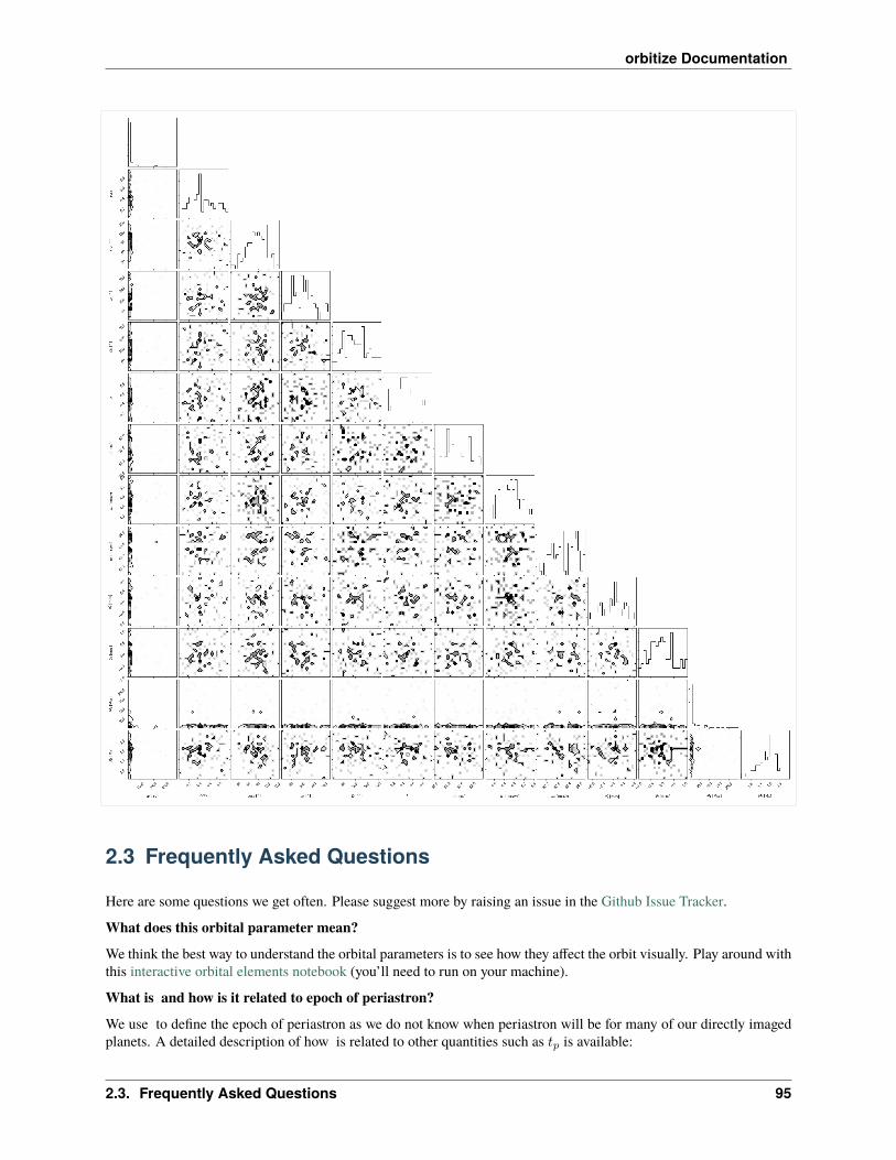
orbitize Documentation
2.3 Frequently Asked Questions
Here are some questions we get often. Please suggest more by raising an issue in the Github Issue Tracker.
What does this orbital parameter mean?
We think the best way to understand the orbital parameters is to see how they affect the orbit visually. Play around withthis interactive orbital elements notebook (you’ll need to run on your machine).
What is and how is it related to epoch of periastron?
We use to define the epoch of periastron as we do not know when periastron will be for many of our directly imagedplanets. A detailed description of how is related to other quantities such as 𝑡𝑝 is available:
2.3. Frequently Asked Questions 95

orbitize Documentation
2.3.1 𝜏 and Time of Periastron
Here, we will discuss what exactly is 𝜏 , the parameter orbitize! uses to parametrize the epoch of periastron, andhow it is related to other quantities of the epoch of periastron in the literature.
Time of Periastron and Motivation for 𝜏
The time (or epoch) of periastron is an important quantity for describing an orbit. It defines when the two orbitingbodies are closest to one another (i.e., when a planet is closest to its star). In many papers in the literature, the epoch ofperiastron is described by 𝑡𝑝, which is literally a date at which periastron occurs. This is a very important date becausewe use this date to anchor our orbit in time.
The value of 𝑡𝑝 is well constrained when we know we observed periastron, which is often the case for radial velociyor transiting exoplanets when the orbital periods are short and our data covers a full orbital period. In those cases,we know approximately when 𝑡𝑝 should be in time, so it is easy to define prior bounds for it. However, in the caseof direct imaging, many of our companions have orbital periods that are orders of magnitude larger than the currentorbital coverage of the data where we do not really know if the next periastron is in years, decades, centuries, or evenmillennia. This is the motivation for 𝜏 .
Definition of 𝜏
𝜏 is a dimentionless quantity between 0 and 1 defined with respect to a reference epoch 𝑡𝑟𝑒𝑓 . For a planet that has a 𝑡𝑝and an orbital period (P), then we define 𝜏 as:
𝜏 =𝑡𝑝 − 𝑡𝑟𝑒𝑓
𝑃.
Because 𝜏 is always between 0 and 1, it is easy to figure out the bounds of 𝜏 whereas if the orbital period is highlyuncertain, it may be difficult to put bounds on 𝑡𝑝 that would encompass all allowable bound orbits.
Relation to 𝑡𝑝
As seen in the above equation, it is relatively straightforward to covert between orbital parameter sets that use 𝜏 and 𝑡𝑝.You just need to know the orbital period and reference epoch. In orbitize!, both the System class and the Resultsclass has the attribute tau_ref_epoch which stores 𝑡𝑟𝑒𝑓 , so there should always be a convenient way to grab thisnumber. By default, we use 𝑡𝑟𝑒𝑓 = 58849 MJD.
One thing to note that is a given orbit has only a single valid 𝜏 , but that an orbit can be defined by many 𝑡𝑝, since theorbit is periodic. Thus, 𝑡𝑝 + 𝑃 is another valid time of periastron.
We also provide some helper functions to covert between 𝑡𝑝 and 𝜏
[1]: import numpy as npimport orbitize.basis
# How to get orbital period in the orbitize! standard basissma = 9 # au, semi-major axismtot = 1.2 # Solar masses, total massperiod = np.sqrt(sma**3/mtot) # years, period
tau = 0.2tau_ref_epoch = 58849
# convert tau to tp(continues on next page)
96 Chapter 2. User Guide:
orbitize Documentation
(continued from previous page)
tp = orbitize.basis.tau_to_tp(tau, tau_ref_epoch, period)
print(tp)
# convert tp back to tautau2 = orbitize.basis.tp_to_tau(tp, tau_ref_epoch, period)
print(tau2)
# convert tau to tp, but pick the first tp after MJD = 0tp_new = orbitize.basis.tau_to_tp(tau, tau_ref_epoch, period, after_date=0)
print(tp_new)
60649.500977158860.20000000000000026634.471662393138
Relation to Mean Anomaly
The mean anomaly (M) of an orbit describes the current orbital phase of a planet. M goes from 0 to 2𝜋, and M =0 means the planet is at periastron. Unlike 𝑡𝑝 and 𝜏 which describe the epoch of periastron, M describes the currentposition of the planet in its orbit.
To compute M of a planet at some time t, we have provided the following helper function:
[2]: # Use the orbit defined in the previous example
t = 60000 # time in MJD when we want to know the M of the particle
M = orbitize.basis.tau_to_manom(t, sma, mtot, tau, tau_ref_epoch)
print(M)
# now compute M for periastronM_peri = orbitize.basis.tau_to_manom(tp, sma, mtot, tau, tau_ref_epoch)
print(M_peri)
5.8298742511508441.3951473992034527e-15
Why is the default prior on inclination a sine prior?
Our goal with the default prior is to have an isotropic distribution of the orbital plane. To obtain this, we use inclinationand position angle of the ascending node (PAN) to define the orbital plane. They actually coorespond to the two anglesin a spherical coordinate system: inclinaion is the polar angle and PAN is the azimuthal angle. Becuase of this choiceof coordinates, there are less orbital configurations near the poles (when inclination is near 0 or 180), so we use a sineprior to downweigh those areas to give us an isotropic distribution. A more detailed discussion of this is here:
2.3. Frequently Asked Questions 97

orbitize Documentation
2.3.2 Defining the orbital plane with 𝑖 and Ω
(Jason Wang, 2021)
Here we discuss how the orbit plane orientation is defined. We also encourage you to play around with this interactiveorbital elements notebook to get a feel for the orbital elements. Also note that we refer to the values of the angles indegrees when discussing them but all angles are in radians in orbitize!.
Inclination (𝑖) and Position angle of the Ascending Node (PAN; Ω) define the plane of the orbit in the sky. Inclinationdescribes the tilt of the orbital plane relative to the plane in the sky, and PAN describes the rotation of the line of nodes,which is the intersection between the orbital plane and the plane of the sky.
An intuitive way to think about it is in terms of spherical coordinates. 𝑖 is equivalent to 𝜃 (range from 0 to 180 deg),and Ω is equivalent to 𝜙 (range from 0 to 360 deg) in common spherical notation. The sphere in this case is tilted, withone of the poles pointed towards us.
Why do we use a sine prior on inclination?
You might also hear about using a uniform prior in cos(𝑖), which is an equivalent statement. We use a sine prioron inclination because our ultimate goal is to have an isotropic prior on the orbital plane, and due to how we choosecoordiantes, this becomes a sine prior on inclination. We can go through some math/visual explaination, but theeasiest is perhaps seeing the distribution of orbital plane orientations on a sphere. We use the orbital plane normal(perpendicular vector from the orbit plane) to define the orientation of the plane in 3D space. The normal points to asingle point on a unit sphere. Isotropic distributions will uniformly cover the unit sphere.
In the exercise below, if we randomly draw orbital plane orientations using either an uniform or sine prior for inclination,you’ll see that the uniform prior causes more points to cluster near the poles, whereas the sine prior is more uniform.Note that generally the edges of the sphere look darker merely due to a viewing angle effect.
[4]: import numpy as npimport matplotlib.pylab as pltfrom orbitize.priors import UniformPrior, SinPrior%matplotlib inline
def spherical_to_xyz(theta, phi, rho=1):"""Transformation with theta and phi in radians"""z = rho * np.cos(theta)x = rho * np.sin(theta) * np.cos(phi)y = rho * np.sin(theta) * np.sin(phi)return x,y,z
fig = plt.figure()
# try a uniform distribution in bothax1 = fig.add_subplot(121, projection='3d')
inc_uni_prior = UniformPrior(0, np.pi)pan_uni_prior = UniformPrior(0, 2*np.pi)
incs_uni = inc_uni_prior.draw_samples(2000)pan_uni = pan_uni_prior.draw_samples(2000)
x_uni, y_uni, z_uni = spherical_to_xyz(incs_uni, pan_uni)(continues on next page)
98 Chapter 2. User Guide:
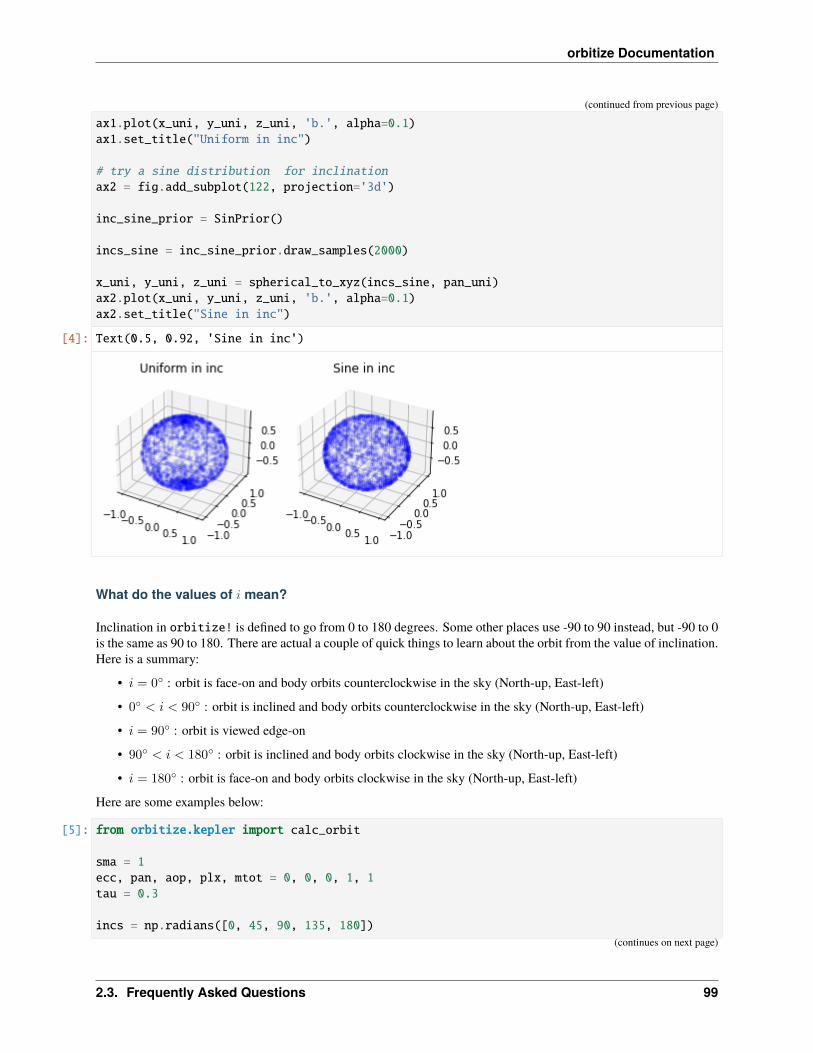
orbitize Documentation
(continued from previous page)
ax1.plot(x_uni, y_uni, z_uni, 'b.', alpha=0.1)ax1.set_title("Uniform in inc")
# try a sine distribution for inclinationax2 = fig.add_subplot(122, projection='3d')
inc_sine_prior = SinPrior()
incs_sine = inc_sine_prior.draw_samples(2000)
x_uni, y_uni, z_uni = spherical_to_xyz(incs_sine, pan_uni)ax2.plot(x_uni, y_uni, z_uni, 'b.', alpha=0.1)ax2.set_title("Sine in inc")
[4]: Text(0.5, 0.92, 'Sine in inc')
What do the values of 𝑖 mean?
Inclination in orbitize! is defined to go from 0 to 180 degrees. Some other places use -90 to 90 instead, but -90 to 0is the same as 90 to 180. There are actual a couple of quick things to learn about the orbit from the value of inclination.Here is a summary:
• 𝑖 = 0∘ : orbit is face-on and body orbits counterclockwise in the sky (North-up, East-left)
• 0∘ < 𝑖 < 90∘ : orbit is inclined and body orbits counterclockwise in the sky (North-up, East-left)
• 𝑖 = 90∘ : orbit is viewed edge-on
• 90∘ < 𝑖 < 180∘ : orbit is inclined and body orbits clockwise in the sky (North-up, East-left)
• 𝑖 = 180∘ : orbit is face-on and body orbits clockwise in the sky (North-up, East-left)
Here are some examples below:
[5]: from orbitize.kepler import calc_orbit
sma = 1ecc, pan, aop, plx, mtot = 0, 0, 0, 1, 1tau = 0.3
incs = np.radians([0, 45, 90, 135, 180])(continues on next page)
2.3. Frequently Asked Questions 99

orbitize Documentation
(continued from previous page)
all_eps = np.linspace(0, 365.25, 200)arc_eps = np.linspace(0, 75, 75)
fig = plt.figure(figsize=(15,4))for i, inc in enumerate(incs):
ax = fig.add_subplot(1, 5, i+1)
all_ras, all_decs, _ = calc_orbit(all_eps, sma, ecc, inc, aop, pan, tau, plx, mtot,→˓tau_ref_epoch=0)
ax.plot(all_ras, all_decs, 'k--', alpha=0.5)
arc_ras, arc_decs, _ = calc_orbit(arc_eps, sma, ecc, inc, aop, pan, tau, plx, mtot,→˓tau_ref_epoch=0)
ax.plot(arc_ras, arc_decs, 'b-', linewidth=2)ax.plot(arc_ras[-1], arc_decs[-1], 'bo', markersize=7)
ax.set_title("i = 0:d deg".format(int(np.degrees(inc))))ax.set_aspect("equal")ax.set_xlim([1.1, -1.1])ax.set_ylim([-1.1, 1.1])ax.set_xlabel("RA")ax.set_ylabel("Dec")
fig.tight_layout()
What do the values of Ω mean?
Ω or PAN defines the rotation of the orbit in the plane of the sky. Increasing PAN will rotate your orbit counterclockwisein the sky. Here are some examples:
[6]: sma = 1ecc, aop, plx, mtot = 0, 0, 1, 1inc = np.pi/4 # 45 degreestau = 0.3
pans = np.radians([0, 30, 90, 150, 270])
all_eps = np.linspace(0, 365.25, 200)arc_eps = np.linspace(0, 75, 75)
fig = plt.figure(figsize=(15,4))(continues on next page)
100 Chapter 2. User Guide:
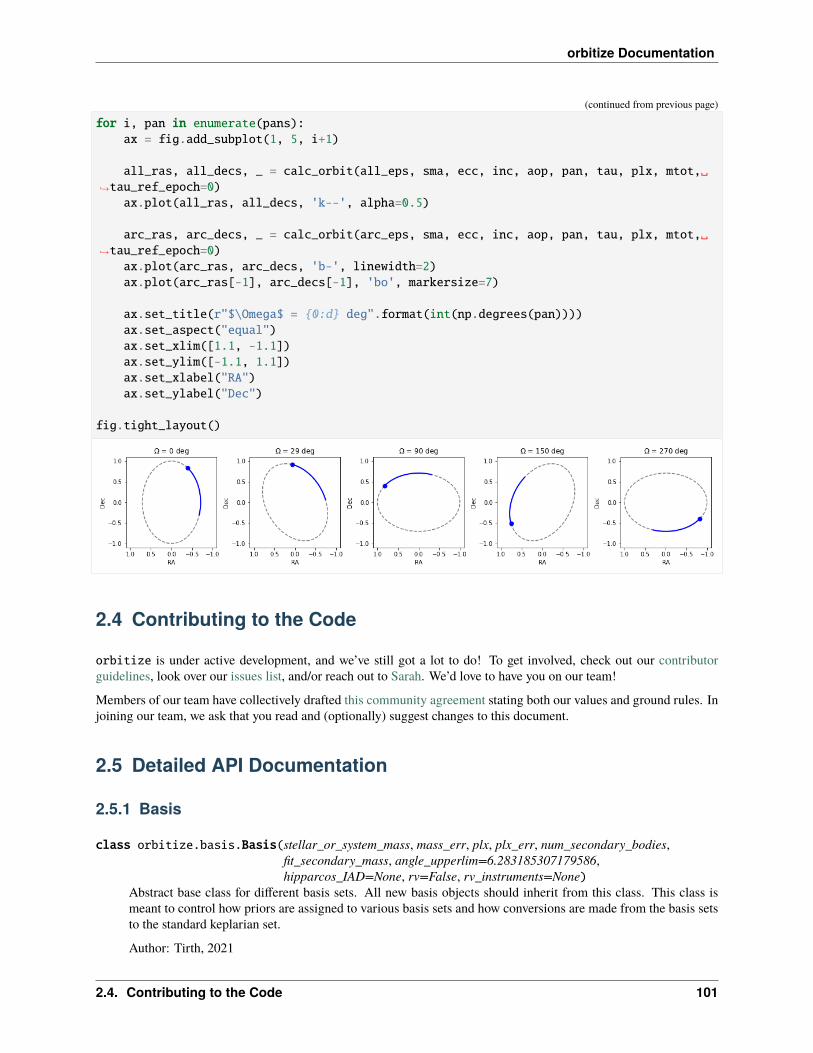
orbitize Documentation
(continued from previous page)
for i, pan in enumerate(pans):ax = fig.add_subplot(1, 5, i+1)
all_ras, all_decs, _ = calc_orbit(all_eps, sma, ecc, inc, aop, pan, tau, plx, mtot,→˓tau_ref_epoch=0)
ax.plot(all_ras, all_decs, 'k--', alpha=0.5)
arc_ras, arc_decs, _ = calc_orbit(arc_eps, sma, ecc, inc, aop, pan, tau, plx, mtot,→˓tau_ref_epoch=0)
ax.plot(arc_ras, arc_decs, 'b-', linewidth=2)ax.plot(arc_ras[-1], arc_decs[-1], 'bo', markersize=7)
ax.set_title(r"$\Omega$ = 0:d deg".format(int(np.degrees(pan))))ax.set_aspect("equal")ax.set_xlim([1.1, -1.1])ax.set_ylim([-1.1, 1.1])ax.set_xlabel("RA")ax.set_ylabel("Dec")
fig.tight_layout()
2.4 Contributing to the Code
orbitize is under active development, and we’ve still got a lot to do! To get involved, check out our contributorguidelines, look over our issues list, and/or reach out to Sarah. We’d love to have you on our team!
Members of our team have collectively drafted this community agreement stating both our values and ground rules. Injoining our team, we ask that you read and (optionally) suggest changes to this document.
2.5 Detailed API Documentation
2.5.1 Basis
class orbitize.basis.Basis(stellar_or_system_mass, mass_err, plx, plx_err, num_secondary_bodies,fit_secondary_mass, angle_upperlim=6.283185307179586,hipparcos_IAD=None, rv=False, rv_instruments=None)
Abstract base class for different basis sets. All new basis objects should inherit from this class. This class ismeant to control how priors are assigned to various basis sets and how conversions are made from the basis setsto the standard keplarian set.
Author: Tirth, 2021
2.4. Contributing to the Code 101
orbitize Documentation
set_default_mass_priors(priors_arr, labels_arr)Adds the necessary priors for the stellar and/or companion masses.
Parameters
• priors_arr (list of orbitize.priors.Prior objects) – holds the prior objectsfor each parameter to be fitted (updated here)
• labels_arr (list of strings) – holds the name of all the parameters to be fitted (up-dated here)
set_hip_iad_priors(priors_arr, labels_arr)Adds the necessary priors relevant to the hipparcos data to ‘priors_arr’ and updates ‘labels_arr’ with thepriors’ corresponding labels.
Parameters
• priors_arr (list of orbitize.priors.Prior objects) – holds the prior objectsfor each parameter to be fitted (updated here)
• labels_arr (list of strings) – holds the name of all the parameters to be fitted (up-dated here)
set_rv_priors(priors_arr, labels_arr)Adds the necessary priors if radial velocity data is supplied to ‘priors_arr’ and updates ‘labels_arr’ with thepriors’ corresponding labels. This function assumes that ‘rv’ data has been supplied and a secondary massis being fitted for.
Parameters
• priors_arr (list of orbitize.priors.Prior objects) – holds the prior objectsfor each parameter to be fitted (updated here)
• labels_arr (list of strings) – holds the name of all the parameters to be fitted (up-dated here)
verify_params()Displays warnings about the ‘fit_secondary_mass’ and ‘rv’ parameters for all basis sets. Can be overridenby any basis class depending on the necessary parameters that need to be checked.
class orbitize.basis.Period(stellar_or_system_mass, mass_err, plx, plx_err, num_secondary_bodies,fit_secondary_mass, angle_upperlim=6.283185307179586,hipparcos_IAD=None, rv=False, rv_instruments=None)
Modification of the standard basis, swapping our sma for period: (per, ecc, inc, aop, pan, tau).
Parameters
• stellar_or_system_mass (float) – mass of the primary star (if fitting for dynamicalmasses of both components) or total system mass (if fitting using relative astrometry only)[M_sol]
• mass_err (float) – uncertainty on ‘stellar_or_system_mass’, in M_sol
• plx (float) – mean parallax of the system, in mas
• plx_err (float) – uncertainty on ‘plx’, in mas
• num_secondary_bodies (int) – number of secondary bodies in the system, should be atleast 1
• fit_secondary_mass (bool) – if True, include the dynamical mass of orbitting body asfitted parameter, if False, ‘stellar_or_system_mass’ is taken to be total mass
102 Chapter 2. User Guide:
orbitize Documentation
• angle_upperlim (float) – either pi or 2pi, to restrict the prior range for ‘pan’ parameter(default: 2pi)
• hipparcos_IAD (orbitize.HipparcosLogProb object) – if not ‘None’, then add rele-vant priors to this data (default: None)
• rv (bool) – if True, then there is radial velocity data and assign radial velocity priors, if False,then there is no radial velocity data and radial velocity priors are not assigned (default: False)
• rv_instruments (np.array) – array of unique rv instruments from the originally supplieddata (default: None)
construct_priors()Generates the parameter label array and initializes the corresponding priors for each parameter that’s to besampled. For the standard basis, the parameters common to each companion are: per, ecc, inc, aop, pan,tau. Parallax, hipparcos (optional), rv (optional), and mass priors are added at the end.
Returns
list: list of strings (labels) that indicate the names of each parameter to sample
list: list of orbitize.priors.Prior objects that indicate the prior distribution of each label
Return type tuple
to_period_basis(param_arr)Convert parameter array from standard basis to period basis by swapping out the semi-major axis parameterto period for each companion. This function is used primarily for testing purposes.
Parameters param_arr (np.array of float) – RxM array of fitting parameters in the stan-dard basis, where R is the number of parameters being fit, and M is the number of orbits. IfM=1 (for MCMC), this can be a 1D array.
Returns
modifies ‘param_arr’ to contain the period for each companion in each orbit rather thansemi-major axis. Shape of ‘param_arr’ remains the same.
Return type np.array of float
to_standard_basis(param_arr)Convert parameter array from period basis to standard basis by swapping out the period parameter to semi-major axis for each companion.
Parameters param_arr (np.array of float) – RxM array of fitting parameters in the periodbasis, where R is the number of parameters being fit, and M is the number of orbits. If M=1(for MCMC), this can be a 1D array.
Returns
modifies ‘param_arr’ to contain the semi-major axis for each companion in each orbitrather than period. Shape of ‘param_arr’ remains the same.
Return type np.array of float
class orbitize.basis.SemiAmp(stellar_or_system_mass, mass_err, plx, plx_err, num_secondary_bodies,fit_secondary_mass, angle_upperlim=6.283185307179586,hipparcos_IAD=None, rv=False, rv_instruments=None)
Modification of the standard basis, swapping our sma for period and additionally sampling in the stellar radialvelocity semi-amplitude: (per, ecc, inc, aop, pan, tau, K).
Note: Ideally, ‘fit_secondary_mass’ is true and rv data is supplied.
2.5. Detailed API Documentation 103
orbitize Documentation
Parameters
• stellar_or_system_mass (float) – mass of the primary star (if fitting for dynamicalmasses of both components) or total system mass (if fitting using relative astrometry only)[M_sol]
• mass_err (float) – uncertainty on ‘stellar_or_system_mass’, in M_sol
• plx (float) – mean parallax of the system, in mas
• plx_err (float) – uncertainty on ‘plx’, in mas
• num_secondary_bodies (int) – number of secondary bodies in the system, should be atleast 1
• fit_secondary_mass (bool) – if True, include the dynamical mass of orbitting body asfitted parameter, if False, ‘stellar_or_system_mass’ is taken to be total mass
• angle_upperlim (float) – either pi or 2pi, to restrict the prior range for ‘pan’ parameter(default: 2*pi)
• hipparcos_IAD (orbitize.HipparcosLogProb object) – if not ‘None’, then add rele-vant priors to this data (default: None)
• rv (bool) – if True, then there is radial velocity data and assign radial velocity priors, if False,then there is no radial velocity data and radial velocity priors are not assigned (default: False)
• rv_instruments (np.array) – array of unique rv instruments from the originally supplieddata (default: None)
compute_companion_mass(period, ecc, inc, semi_amp, m0)Computes a single companion’s mass given period, eccentricity, inclination, stellar rv semi-amplitude, andstellar mass. Uses scipy.fsolve to compute the masses numerically.
Parameters
• period (np.array of float) – the period values for each orbit for a single companion(can be float)
• ecc (np.array of float) – the eccentricity values for each orbit for a single companion(can be float)
• inc (np.array of float) – the inclination values for each orbit for a single companion(can be float)
• semi_amp (np.array of float) – the stellar rv-semi amp values for each orbit (can befloat)
• m0 (np.array of float) – the stellar mass for each orbit (can be float)
Returns the companion mass values for each orbit (can also just be a single float)
Return type np.array of float
compute_companion_sma(period, m0, m_n)Computes a single companion’s semi-major axis using Kepler’s Third Law for each orbit.
Parameters
• period (np.array of float) – the period values for each orbit for a single companion(can be float)
• m0 (np.array of float) – the stellar mass for each orbit (can be float)
• m_n (np.array of float) – the companion mass for each orbit (can be float)
104 Chapter 2. User Guide:
orbitize Documentation
Returns the semi-major axis values for each orbit
Return type np.array of float
construct_priors()Generates the parameter label array and initializes the corresponding priors for each parameter that’s to besampled. For the semi-amp basis, the parameters common to each companion are: per, ecc, inc, aop, pan,tau, K (stellar rv semi-amplitude). Parallax, hipparcos (optional), rv (optional), and mass priors are addedat the end.
The mass parameter will always be m0.
Returns
list: list of strings (labels) that indicate the names of each parameter to sample
list: list of orbitize.priors.Prior objects that indicate the prior distribution of each label
Return type tuple
func(x, lhs, m0)Define function for scipy.fsolve to use when computing companion mass.
Parameters
• x (float) – the companion mass to be calculated (Msol)
• lhs (float) – the left hand side of the rv semi-amplitude equation (Msol^(1/3))
• m0 (float) – the stellar mass (Msol)
Returns
the difference between the rhs and lhs of the rv semi-amplitude equation, ‘x’ is a goodcompanion mass when this difference is very close to zero
Return type float
to_semi_amp_basis(param_arr)Convert parameter array from standard basis to semi-amp basis by swapping out the semi-major axis pa-rameter to period for each companion and computing the stellar rv semi-amplitudes for each companion.
Parameters param_arr (np.array of float) – RxM array of fitting parameters in the periodbasis, where R is the number of parameters being fit, and M is the number of orbits. If M=1(for MCMC), this can be a 1D array.
Returns
modifies ‘param_arr’ to contain the semi-major axis for each companion in each orbitrather than period, appends stellar rv semi-amplitude parameters, and removes compan-ion masses
Return type np.array of float
to_standard_basis(param_arr)Convert parameter array from semi-amp basis to standard basis by swapping out the period parameter tosemi-major axis for each companion and computing the masses of each companion.
Parameters param_arr (np.array of float) – RxM array of fitting parameters in the periodbasis, where R is the number of parameters being fit, and M is the number of orbits. If M=1(for MCMC), this can be a 1D array.
Returns
2.5. Detailed API Documentation 105

orbitize Documentation
modifies ‘param_arr’ to contain the semi-major axis for each companion in each orbitrather than period, removes stellar rv semi-amplitude parameters for each companion, andappends the companion masses to ‘param_arr’
Return type np.array of float
verify_params()Additionally warns that this basis will sample stellar mass rather than sample mass regardless of whether‘fit_secondary_mass’ is True or not.
class orbitize.basis.Standard(stellar_or_system_mass, mass_err, plx, plx_err, num_secondary_bodies,fit_secondary_mass, angle_upperlim=6.283185307179586,hipparcos_IAD=None, rv=False, rv_instruments=None)
Standard basis set based upon the 6 standard Keplarian elements: (sma, ecc, inc, aop, pan, tau).
Parameters
• stellar_or_system_mass (float) – mass of the primary star (if fitting for dynamicalmasses of both components) or total system mass (if fitting using relative astrometry only)[M_sol]
• mass_err (float) – uncertainty on ‘stellar_or_system_mass’, in M_sol
• plx (float) – mean parallax of the system, in mas
• plx_err (float) – uncertainty on ‘plx’, in mas
• num_secondary_bodies (int) – number of secondary bodies in the system, should be atleast 1
• fit_secondary_mass (bool) – if True, include the dynamical mass of orbitting body asfitted parameter, if False, ‘stellar_or_system_mass’ is taken to be total mass
• angle_upperlim (float) – either pi or 2pi, to restrict the prior range for ‘pan’ parameter(default: 2pi)
• hipparcos_IAD (orbitize.HipparcosLogProb object) – if not ‘None’, then add rele-vant priors to this data (default: None)
• rv (bool) – if True, then there is radial velocity data and assign radial velocity priors, if False,then there is no radial velocity data and radial velocity priors are not assigned (default: False)
• rv_instruments (np.array) – array of unique rv instruments from the originally supplieddata (default: None)
construct_priors()Generates the parameter label array and initializes the corresponding priors for each parameter that’s to besampled. For the standard basis, the parameters common to each companion are: sma, ecc, inc, aop, pan,tau. Parallax, hipparcos (optional), rv (optional), and mass priors are added at the end.
Returns
list: list of strings (labels) that indicate the names of each parameter to sample
list: list of orbitize.priors.Prior objects that indicate the prior distribution of each label
Return type tuple
to_standard_basis(param_arr)For standard basis, no conversion needs to be made.
Parameters param_arr (np.array of float) – RxM array of fitting parameters in the stan-dard basis, where R is the number of parameters being fit, and M is the number of orbits. IfM=1 (for MCMC), this can be a 1d array.
106 Chapter 2. User Guide:
orbitize Documentation
Returns param_arr without any modification
Return type np.array of float
class orbitize.basis.XYZ(stellar_or_system_mass, mass_err, plx, plx_err, num_secondary_bodies,fit_secondary_mass, data_table, best_epoch_idx, epochs,angle_upperlim=6.283185307179586, hipparcos_IAD=None, rv=False,rv_instruments=None)
Defines an orbit using the companion’s position and velocity components in XYZ space (x, y, z, xdot, ydot,zdot). The conversion algorithms used for this basis are defined in the following paper: http://www.dept.aoe.vt.edu/~lutze/AOE4134/9OrbitInSpace.pdf
Note: Does not have support with sep,pa data yet.
Note: Does not work for all multi-body data.
Parameters
• stellar_or_system_mass (float) – mass of the primary star (if fitting for dynamicalmasses of both components) or total system mass (if fitting using relative astrometry only)[M_sol]
• mass_err (float) – uncertainty on ‘stellar_or_system_mass’, in M_sol
• plx (float) – mean parallax of the system, in mas
• plx_err (float) – uncertainty on ‘plx’, in mas
• num_secondary_bodies (int) – number of secondary bodies in the system, should be atleast 1
• fit_secondary_mass (bool) – if True, include the dynamical mass of orbitting body asfitted parameter, if False, ‘stellar_or_system_mass’ is taken to be total mass
• input_table (astropy.table.Table) – output from ‘orbitize.read_input.read_file()’
• best_epoch_idx (list) – indices of the epochs corresponding to the smallest uncertainties
• epochs (list) – all of the astrometric epochs from ‘input_table’
• angle_upperlim (float) – either pi or 2pi, to restrict the prior range for ‘pan’ parameter(default: 2*pi)
• hipparcos_IAD (orbitize.HipparcosLogProb object) – if not ‘None’, then add rele-vant priors to this data (default: None)
• rv (bool) – if True, then there is radial velocity data and assign radial velocity priors, if False,then there is no radial velocity data and radial velocity priors are not assigned (default: False)
• rv_instruments (np.array) – array of unique rv instruments from the originally supplieddata (default: None)
Author: Rodrigo
construct_priors()Generates the parameter label array and initializes the corresponding priors for each parameter that’s tobe sampled. For the xyz basis, the parameters common to each companion are: x, y, z, xdot, ydot, zdot.Parallax, hipparcos (optional), rv (optional), and mass priors are added at the end.
2.5. Detailed API Documentation 107
orbitize Documentation
The xyz basis describes the position and velocity vectors with reference to the local coordinate system (theorigin of the system is star).
Returns
list: list of strings (labels) that indicate the names of each parameter to sample
list: list of orbitize.priors.Prior objects that indicate the prior distribution of each label
Return type tuple
standard_to_xyz(epoch, elems, tau_ref_epoch=58849, tolerance=1e-09, max_iter=100)Converts array of orbital elements from the regular base of Keplerian orbits to positions and velocities inxyz Uses code from orbitize.kepler
Parameters
• epoch (float) – Date in MJD of observation to calculate time of periastron passage (tau).
• elems (np.array of floats) – Orbital elements (sma, ecc, inc, aop, pan, tau, plx, mtot).If more than 1 set of parameters is passed, the first dimension must be the number of orbitalparameter sets, and the second the orbital elements.
Returns
Orbital elements in xyz (x-coordinate [au], y-coordinate [au], z-coordinate [au], velocity in x[km/s], velocity in y [km/s], velocity in z [km/s], parallax [mas], total mass of the two-bodyorbit
(M_* + M_planet) [Solar masses])
Return type np.array
to_standard_basis(param_arr)Makes a call to ‘xyz_to_standard’ to convert each companion’s xyz parameters to the standard parametersan returns the updated array for conversion.
Parameters param_arr (np.array of float) – RxM array of fitting parameters in the periodbasis, where R is the number of parameters being fit, and M is the number of orbits. If M=1(for MCMC), this can be a 1D array.
Returns Orbital elements in the standard basis for all companions.
Return type np.array
to_xyz_basis(param_arr)Makes a call to ‘standard_to_xyz’ to convert each companion’s standard keplerian parameters to the xyzparameters an returns the updated array for conversion.
Parameters param_arr (np.array of float) – RxM array of fitting parameters in the periodbasis, where R is the number of parameters being fit, and M is the number of orbits. If M=1(for MCMC), this can be a 1D array.
Returns Orbital elements in the xyz for all companions.
Return type np.array
verify_params()For now, additionally throws exceptions if data is supplied in sep/pa or if the best epoch for each body isone of the last two (which would inevtably mess up how the priors are imposed).
xyz_to_standard(epoch, elems, tau_ref_epoch=58849)Converts array of orbital elements in terms of position and velocity in xyz to the standard basis.
Parameters
108 Chapter 2. User Guide:

orbitize Documentation
• epoch (float) – Date in MJD of observation to calculate time of periastron passage (tau).
• elems (np.array of floats) – Orbital elements in xyz basis (x-coordinate [au], y-coordinate [au], z-coordinate [au], velocity in x [km/s], velocity in y [km/s], velocity in z[km/s], parallax [mas], total mass of the two-body orbit (M_* + M_planet) [Solar masses]).If more than 1 set of parameters is passed, the first dimension must be the number of orbitalparameter sets, and the second the orbital elements.
Returns
Orbital elements in the standard basis (sma, ecc, inc, aop, pan, tau, plx, mtot)
Return type np.array
orbitize.basis.switch_tau_epoch(old_tau, old_epoch, new_epoch, period)Convert tau to another tau that uses a different referench epoch
Parameters
• old_tau (float or np.array) – old tau to convert
• old_epoch (float or np.array) – old reference epoch (days, typically MJD)
• new_epoch (float or np.array) – new reference epoch (days, same system asold_epoch)
• period (float or np.array) – orbital period (years)
Returns new taus
Return type float or np.array
orbitize.basis.tau_to_manom(date, sma, mtot, tau, tau_ref_epoch)Gets the mean anomlay. Wrapper for kepler.tau_to_manom, kept here for backwards compatibility.
Parameters
• date (float or np.array) – MJD
• sma (float) – semi major axis (AU)
• mtot (float) – total mass (M_sun)
• tau (float) – epoch of periastron, in units of the orbital period
• tau_ref_epoch (float) – reference epoch for tau
Returns mean anomaly on that date [0, 2pi)
Return type float or np.array
orbitize.basis.tau_to_tp(tau, ref_epoch, period, after_date=None)Convert tau (epoch of periastron in fractional orbital period after ref epoch) to t_p (date in days, usually MJD,but works with whatever system ref_epoch is given in)
Parameters
• tau (float or np.array) – value of tau to convert
• ref_epoch (float or np.array) – date (in days, typically MJD) that tau is defined rel-ative to
• period (float or np.array) – period (in years) that tau is noralized with
• after_date (float) – tp will be the first periastron after this date. If None, use ref_epoch.
Returns corresponding t_p of the taus
2.5. Detailed API Documentation 109
orbitize Documentation
Return type float or np.array
orbitize.basis.tp_to_tau(tp, ref_epoch, period)Convert t_p to tau
Parameters
• tp (float or np.array) – value to t_p to convert (days, typically MJD)
• ref_epoch (float or np.array) – reference epoch (in days) that tau is defined from.Same system as tp (e.g., MJD)
• period (float or np.array) – period (in years) that tau is defined by
Returns corresponding taus
Return type float or np.array
2.5.2 Driver
class orbitize.driver.Driver(input_data, sampler_str, num_secondary_bodies, stellar_or_system_mass, plx,mass_err=0, plx_err=0, lnlike='chi2_lnlike', system_kwargs=None,mcmc_kwargs=None)
Runs through orbitize methods in a standardized way.
Parameters
• input_data – Either a relative path to data file or astropy.table.Table object in the orbitizeformat. See orbitize.read_input
• sampler_str (str) – algorithm to use for orbit computation. “MCMC” for Markov ChainMonte Carlo, “OFTI” for Orbits for the Impatient
• num_secondary_bodies (int) – number of secondary bodies in the system. Should be atleast 1.
• stellar_or_system_mass (float) – mass of the primary star (if fitting for dynamicalmasses of both components) or total system mass (if fitting using relative astrometry only)[M_sol]
• plx (float) – mean parallax of the system [mas]
• mass_err (float, optional) – uncertainty on stellar_or_system_mass [M_sol]
• plx_err (float, optional) – uncertainty on plx [mas]
• lnlike (str, optional) – name of function in orbitize.lnlike that will be used tocompute likelihood. (default=”chi2_lnlike”)
• system_kwargs (dict, optional) – restrict_angle_ranges, tau_ref_epoch,fit_secondary_mass, hipparcos_IAD, gaia, use_rebound, fitting_basis fororbitize.system.System.
• mcmc_kwargs (dict, optional) – num_temps, num_walkers, and num_threadskwargs for orbitize.sampler.MCMC
Written: Sarah Blunt, 2018
110 Chapter 2. User Guide:

orbitize Documentation
2.5.3 Gaia API Module
class orbitize.gaia.GaiaLogProb(gaia_num, hiplogprob, dr='dr2')Class to compute the log probability of an orbit with respect to a single astrometric position point from Gaia.Uses astroquery to look up Gaia astrometric data, and computes log-likelihood. To be used in conjunction withorbitize.hipparcos.HipLogProb; see documentation for that object for more detail.
Follows Nielsen+ 2020 (studying the orbit of beta Pic b). Note that this class currently only fits for the positionof the star in the Gaia epoch, not the star’s proper motion.
Note: In orbitize, it is possible to perform a fit to just the Hipparcos IAD, but not to just the Gaia astrometricdata.
Parameters
• gaia_num (int) – the Gaia source ID of the object you’re fitting. Note that the dr2 and edr3source IDs are not necessarily the same.
• hiplogprob (orbitize.hipparcos.HipLogProb) – object containing all info relevant toHipparcos IAD fitting
• dr (str) – either ‘dr2’ or ‘edr3’
Written: Sarah Blunt, 2021
compute_lnlike(raoff_model, deoff_model, samples, param_idx)Computes the log likelihood of an orbit model with respect to a single Gaia astrometric point. This is addedto the likelihoods calculated with respect to other data types in sampler._logl().
Parameters
• raoff_model (np.array of float) – 2xM primary RA offsets from the barycenter in-curred from orbital motion of companions (i.e. not from parallactic motion), where Mis the number of orbits being tested, and raoff_model[0,:] are position predictions at theHipparcos epoch, and raoff_model[1,:] are position predictions at the Gaia epoch
• deoff_model (np.array of float) – 2xM primary decl offsets from the barycenterincurred from orbital motion of companions (i.e. not from parallactic motion), where Mis the number of orbits being tested, and deoff_model[0,:] are position predictions at theHipparcos epoch, and deoff_model[1,:] are position predictions at the Gaia epoch
• samples (np.array of float) – R-dimensional array of fitting parameters, where R isthe number of parameters being fit. Must be in the same order documented in System.
• param_idx – a dictionary matching fitting parameter labels to their indices in an array offitting parameters (generally set to System.basis.param_idx).
Returns
array of length M, where M is the number of input orbits, representing the log likelihoodof each orbit with respect to the Gaia position measurement.
Return type np.array of float
2.5. Detailed API Documentation 111
orbitize Documentation
2.5.4 Hipparcos API Module
class orbitize.hipparcos.HipparcosLogProb(path_to_iad_file, hip_num, num_secondary_bodies,alphadec0_epoch=1991.25, renormalize_errors=False)
Class to compute the log probability of an orbit with respect to the Hipparcos Intermediate Astrometric Data(IAD). Queries Vizier for all metadata relevant to the IAD, and reads in the IAD themselves from a specifiedlocation. Follows Nielsen+ 2020 (studying the orbit of beta Pic b).
Fitting the Hipparcos IAD requires fitting for the following five parameters. They are added to the vector offitting parameters in system.py, but are described here for completeness. See Nielsen+ 2020 for more detail.
• alpha0: RA offset from the reported Hipparcos position at a particular epoch (usually 1991.25)[mas]
• delta0: Dec offset from the reported Hipparcos position at a particular epoch (usually 1991.25)[mas]
• pm_ra: RA proper motion [mas/yr]
• pm_dec: Dec proper motion [mas/yr]
• plx: parallax [mas]
Note: In orbitize, it is possible to perform a fit to just the Hipparcos IAD, but not to just the Gaia astrometricdata.
Parameters
• path_to_iad_file (str) – location of IAD file to be used in your fit. See the Hipparcostutorial for a walkthrough of how to download these files.
• hip_num (str) – Hipparcos ID of star. Available on Simbad. Should have zeros in the prefixif number is <100,000. (i.e. 27321 should be passed in as ‘027321’).
• num_secondary_bodies (int) – number of companions in the system
• alphadec0_epoch (float) – epoch (in decimal year) that the fitting parameters alpha0 anddelta0 are defined relative to (see above).
• renormalize_errors (bool) – if True, normalize the scan errors to get chisq_red = 1,following Nielsen+ 2020 (eq 10). In general, this should be False, but it’s helpful for testing.Check out orbitize.hipparcos.nielsen_iad_refitting_test() for an example using this renormal-ization.
Written: Sarah Blunt & Rob de Rosa, 2021
compute_lnlike(raoff_model, deoff_model, samples, param_idx)Computes the log likelihood of an orbit model with respect to the Hipparcos IAD. This is added to thelikelihoods calculated with respect to other data types in sampler._logl().
Parameters
• raoff_model (np.array of float) – M-dimensional array of primary RA offsets fromthe barycenter incurred from orbital motion of companions (i.e. not from parallactic mo-tion), where M is the number of epochs of IAD scan data.
• deoff_model (np.array of float) – M-dimensional array of primary RA offsets fromthe barycenter incurred from orbital motion of companions (i.e. not from parallactic mo-tion), where M is the number of epochs of IAD scan data.
112 Chapter 2. User Guide:
orbitize Documentation
• samples (np.array of float) – R-dimensional array of fitting parameters, where R isthe number of parameters being fit. Must be in the same order documented in System.
• param_idx – a dictionary matching fitting parameter labels to their indices in an array offitting parameters (generally set to System.basis.param_idx).
Returns
array of length M, where M is the number of input orbits, representing the log likelihoodof each orbit with respect to the Hipparcos IAD.
Return type np.array of float
orbitize.hipparcos.nielsen_iad_refitting_test(iad_file, hip_num='027321',saveplot='bPic_IADrefit.png', burn_steps=100,mcmc_steps=5000)
Reproduce the IAD refitting test from Nielsen+ 2020 (end of Section 3.1). The default MCMC parameters arewhat you’d want to run before using the IAD for a new system. This fit uses 100 walkers.
Parameters
• iad_loc (str) – path to the IAD file.
• hip_num (str) – Hipparcos ID of star. Available on Simbad. Should have zeros in the prefixif number is <100,000. (i.e. 27321 should be passed in as ‘027321’).
• saveplot (str) – what to save the summary plot as. If None, don’t make a plot
• burn_steps (int) – number of MCMC burn-in steps to run.
• mcmc_steps (int) – number of MCMC production steps to run.
Returns
numpy.array of float: n_steps x 5 array of posterior samples
orbitize.hipparcos.HipparcosLogProb: the object storing relevant metadata for the per-formed Hipparcos IAD fit
Return type tuple
2.5.5 Kepler Solver
This module solves for the orbit of the planet given Keplerian parameters.
orbitize.kepler.calc_orbit(epochs, sma, ecc, inc, aop, pan, tau, plx, mtot, mass_for_Kamp=None,tau_ref_epoch=58849, tolerance=1e-09, max_iter=100, use_c=True,use_gpu=False)
Returns the separation and radial velocity of the body given array of orbital parameters (size n_orbs) at givenepochs (array of size n_dates)
Based on orbit solvers from James Graham and Rob De Rosa. Adapted by Jason Wang and Henry Ngo.
Parameters
• epochs (np.array) – MJD times for which we want the positions of the planet
• sma (np.array) – semi-major axis of orbit [au]
• ecc (np.array) – eccentricity of the orbit [0,1]
• inc (np.array) – inclination [radians]
• aop (np.array) – argument of periastron [radians]
2.5. Detailed API Documentation 113
orbitize Documentation
• pan (np.array) – longitude of the ascending node [radians]
• tau (np.array) – epoch of periastron passage in fraction of orbital period past MJD=0 [0,1]
• plx (np.array) – parallax [mas]
• mtot (np.array) – total mass of the two-body orbit (M_* + M_planet) [Solar masses]
• mass_for_Kamp (np.array, optional) – mass of the body that causes the RV signal. Forexample, if you want to return the stellar RV, this is the planet mass. If you want to return theplanetary RV, this is the stellar mass. [Solar masses]. For planet mass ~ 0, mass_for_Kamp~ M_tot, and function returns planetary RV (default).
• tau_ref_epoch (float, optional) – reference date that tau is defined with respect to(i.e., tau=0)
• tolerance (float, optional) – absolute tolerance of iterative computation. Defaults to1e-9.
• max_iter (int, optional) – maximum number of iterations before switching. Defaultsto 100.
• use_c (bool, optional) – Use the C solver if configured. Defaults to True
• use_gpu (bool, optional) – Use the GPU solver if configured. Defaults to False
Returns
raoff (np.array): array-like (n_dates x n_orbs) of RA offsets between the bodies (origin is at theother body) [mas]
deoff (np.array): array-like (n_dates x n_orbs) of Dec offsets between the bodies [mas]
vz (np.array): array-like (n_dates x n_orbs) of radial velocity of one of the bodies (seemass_for_Kamp description) [km/s]
Return type 3-tuple
Written: Jason Wang, Henry Ngo, 2018
orbitize.kepler.tau_to_manom(date, sma, mtot, tau, tau_ref_epoch)Gets the mean anomlay
Parameters
• date (float or np.array) – MJD
• sma (float) – semi major axis (AU)
• mtot (float) – total mass (M_sun)
• tau (float) – epoch of periastron, in units of the orbital period
• tau_ref_epoch (float) – reference epoch for tau
Returns mean anomaly on that date [0, 2pi)
Return type float or np.array
114 Chapter 2. User Guide:
orbitize Documentation
2.5.6 Log(Likelihood)
orbitize.lnlike.chi2_lnlike(data, errors, corrs, model, jitter, seppa_indices)Compute Log of the chi2 Likelihood
Parameters
• data (np.array) – Nobsx2 array of data, where data[:,0] = sep/RA/RV for every epoch,and data[:,1] = corresponding pa/DEC/np.nan.
• errors (np.array) – Nobsx2 array of errors for each data point. Same format as data.
• corrs (np.array) – Nobs array of Pearson correlation coeffs between the two quantities.If there is none, can be None.
• model (np.array) – Nobsx2xM array of model predictions, where M is the number of orbitsbeing compared against the data. If M is 1, model can be 2 dimensional.
• jitter (np.array) – Nobsx2xM array of jitter values to add to errors. Elements of arrayshould be 0 for for all data other than stellar rvs.
• seppa_indices (list) – list of epoch numbers whose observations are given in sep/PA.This list is located in System.seppa.
Returns Nobsx2xM array of chi-squared values.
Return type np.array
Note: Example: We have 8 epochs of data for a system. OFTI returns an array of 10,000 sets of orbitalparameters. The model input for this function should be an array of dimension 8 x 2 x 10,000.
orbitize.lnlike.chi2_norm_term(errors, corrs)Return only the normalization term of the Gaussian likelihood:
−𝑙𝑜𝑔(√
(2𝜋 * 𝑒𝑟𝑟𝑜𝑟2))
or
−0.5 * (𝑙𝑜𝑔(𝑑𝑒𝑡(𝐶)) + 𝑁 * 𝑙𝑜𝑔(2𝜋))
Parameters
• errors (np.array) – Nobsx2 array of errors for each data point. Same format as data.
• corrs (np.array) – Nobs array of Pearson correlation coeffs between the two quantities.If there is none, can be None.
Returns sum of the normalization terms
Return type float
2.5. Detailed API Documentation 115
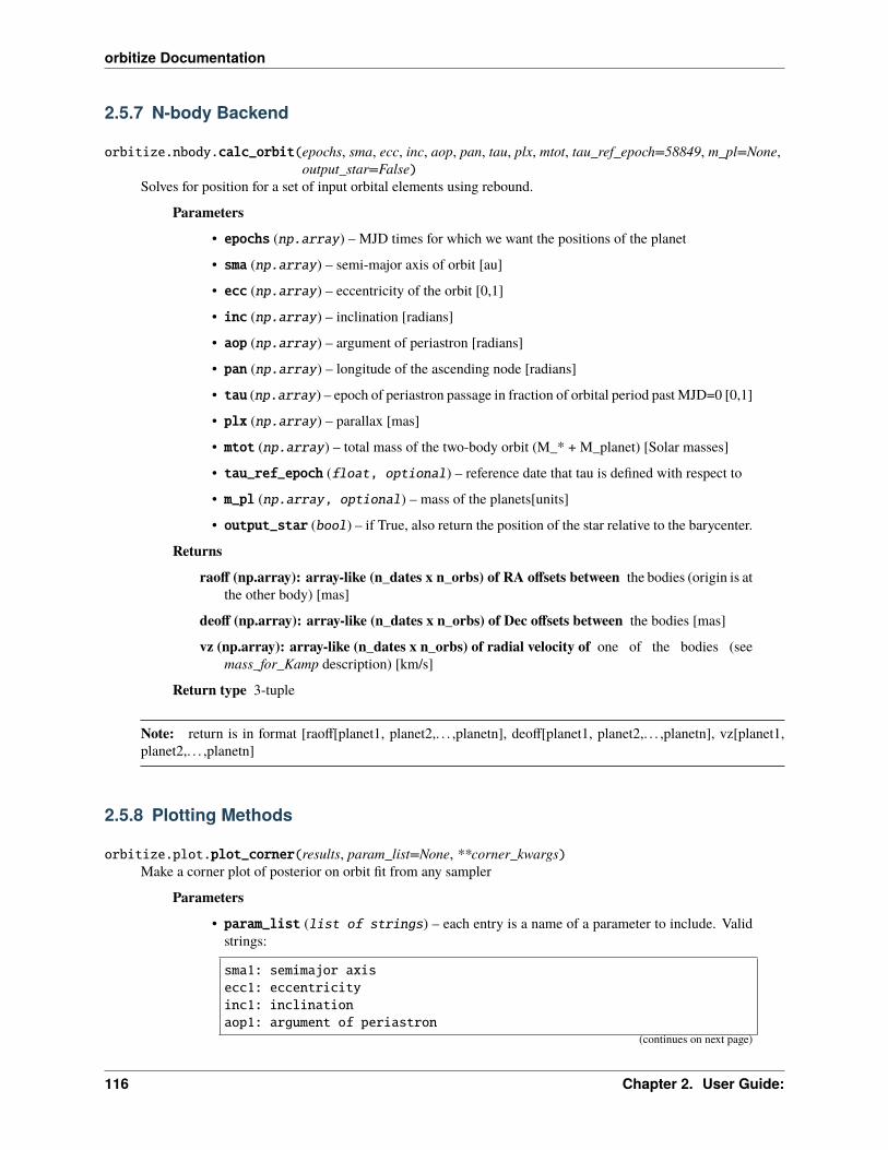
orbitize Documentation
2.5.7 N-body Backend
orbitize.nbody.calc_orbit(epochs, sma, ecc, inc, aop, pan, tau, plx, mtot, tau_ref_epoch=58849, m_pl=None,output_star=False)
Solves for position for a set of input orbital elements using rebound.
Parameters
• epochs (np.array) – MJD times for which we want the positions of the planet
• sma (np.array) – semi-major axis of orbit [au]
• ecc (np.array) – eccentricity of the orbit [0,1]
• inc (np.array) – inclination [radians]
• aop (np.array) – argument of periastron [radians]
• pan (np.array) – longitude of the ascending node [radians]
• tau (np.array) – epoch of periastron passage in fraction of orbital period past MJD=0 [0,1]
• plx (np.array) – parallax [mas]
• mtot (np.array) – total mass of the two-body orbit (M_* + M_planet) [Solar masses]
• tau_ref_epoch (float, optional) – reference date that tau is defined with respect to
• m_pl (np.array, optional) – mass of the planets[units]
• output_star (bool) – if True, also return the position of the star relative to the barycenter.
Returns
raoff (np.array): array-like (n_dates x n_orbs) of RA offsets between the bodies (origin is atthe other body) [mas]
deoff (np.array): array-like (n_dates x n_orbs) of Dec offsets between the bodies [mas]
vz (np.array): array-like (n_dates x n_orbs) of radial velocity of one of the bodies (seemass_for_Kamp description) [km/s]
Return type 3-tuple
Note: return is in format [raoff[planet1, planet2,. . . ,planetn], deoff[planet1, planet2,. . . ,planetn], vz[planet1,planet2,. . . ,planetn]
2.5.8 Plotting Methods
orbitize.plot.plot_corner(results, param_list=None, **corner_kwargs)Make a corner plot of posterior on orbit fit from any sampler
Parameters
• param_list (list of strings) – each entry is a name of a parameter to include. Validstrings:
sma1: semimajor axisecc1: eccentricityinc1: inclinationaop1: argument of periastron
(continues on next page)
116 Chapter 2. User Guide:
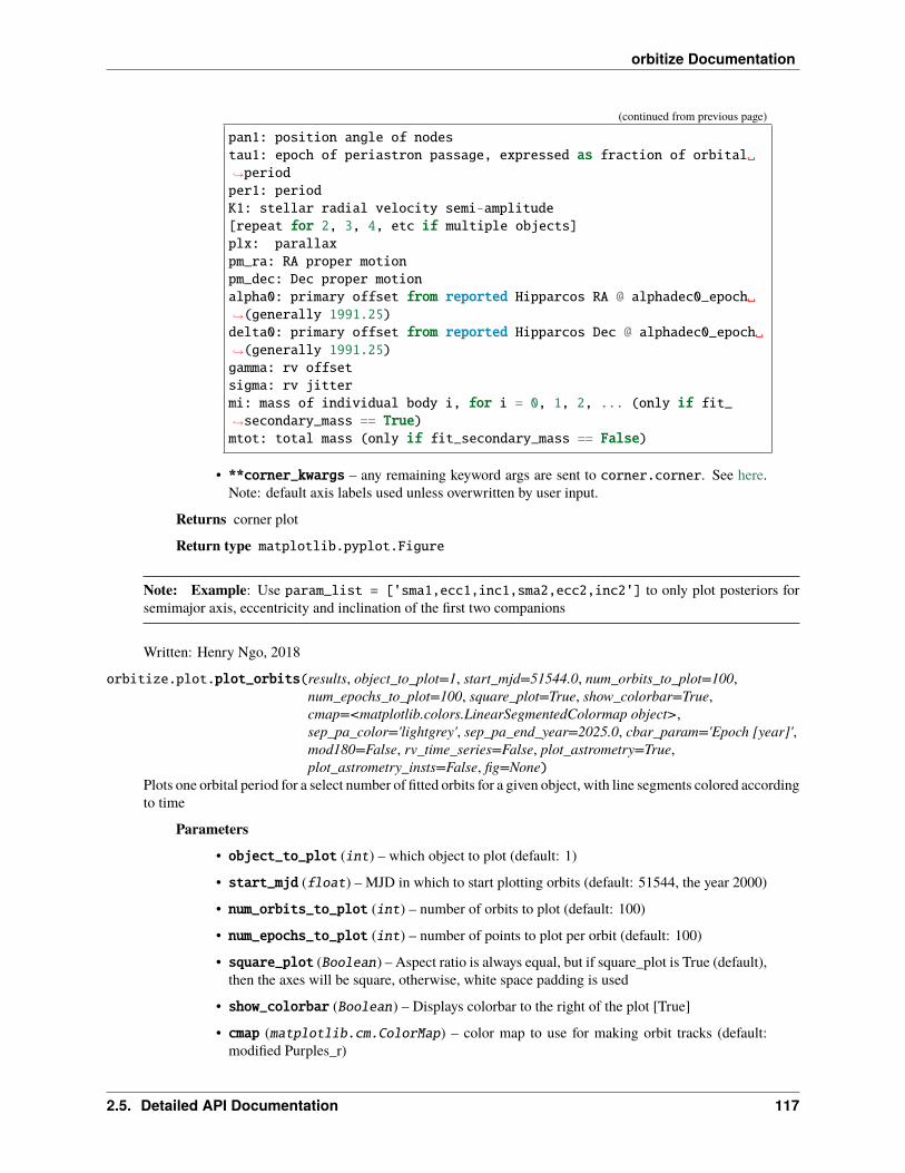
orbitize Documentation
(continued from previous page)
pan1: position angle of nodestau1: epoch of periastron passage, expressed as fraction of orbital→˓periodper1: periodK1: stellar radial velocity semi-amplitude[repeat for 2, 3, 4, etc if multiple objects]plx: parallaxpm_ra: RA proper motionpm_dec: Dec proper motionalpha0: primary offset from reported Hipparcos RA @ alphadec0_epoch→˓(generally 1991.25)delta0: primary offset from reported Hipparcos Dec @ alphadec0_epoch→˓(generally 1991.25)gamma: rv offsetsigma: rv jittermi: mass of individual body i, for i = 0, 1, 2, ... (only if fit_→˓secondary_mass == True)mtot: total mass (only if fit_secondary_mass == False)
• **corner_kwargs – any remaining keyword args are sent to corner.corner. See here.Note: default axis labels used unless overwritten by user input.
Returns corner plot
Return type matplotlib.pyplot.Figure
Note: Example: Use param_list = ['sma1,ecc1,inc1,sma2,ecc2,inc2'] to only plot posteriors forsemimajor axis, eccentricity and inclination of the first two companions
Written: Henry Ngo, 2018
orbitize.plot.plot_orbits(results, object_to_plot=1, start_mjd=51544.0, num_orbits_to_plot=100,num_epochs_to_plot=100, square_plot=True, show_colorbar=True,cmap=<matplotlib.colors.LinearSegmentedColormap object>,sep_pa_color='lightgrey', sep_pa_end_year=2025.0, cbar_param='Epoch [year]',mod180=False, rv_time_series=False, plot_astrometry=True,plot_astrometry_insts=False, fig=None)
Plots one orbital period for a select number of fitted orbits for a given object, with line segments colored accordingto time
Parameters
• object_to_plot (int) – which object to plot (default: 1)
• start_mjd (float) – MJD in which to start plotting orbits (default: 51544, the year 2000)
• num_orbits_to_plot (int) – number of orbits to plot (default: 100)
• num_epochs_to_plot (int) – number of points to plot per orbit (default: 100)
• square_plot (Boolean) – Aspect ratio is always equal, but if square_plot is True (default),then the axes will be square, otherwise, white space padding is used
• show_colorbar (Boolean) – Displays colorbar to the right of the plot [True]
• cmap (matplotlib.cm.ColorMap) – color map to use for making orbit tracks (default:modified Purples_r)
2.5. Detailed API Documentation 117
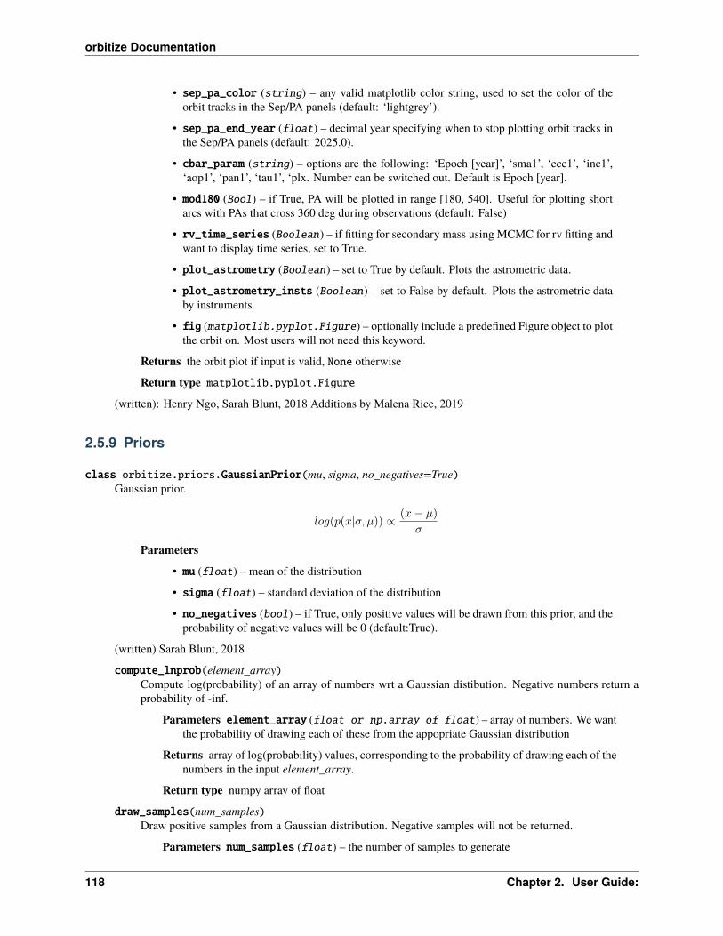
orbitize Documentation
• sep_pa_color (string) – any valid matplotlib color string, used to set the color of theorbit tracks in the Sep/PA panels (default: ‘lightgrey’).
• sep_pa_end_year (float) – decimal year specifying when to stop plotting orbit tracks inthe Sep/PA panels (default: 2025.0).
• cbar_param (string) – options are the following: ‘Epoch [year]’, ‘sma1’, ‘ecc1’, ‘inc1’,‘aop1’, ‘pan1’, ‘tau1’, ‘plx. Number can be switched out. Default is Epoch [year].
• mod180 (Bool) – if True, PA will be plotted in range [180, 540]. Useful for plotting shortarcs with PAs that cross 360 deg during observations (default: False)
• rv_time_series (Boolean) – if fitting for secondary mass using MCMC for rv fitting andwant to display time series, set to True.
• plot_astrometry (Boolean) – set to True by default. Plots the astrometric data.
• plot_astrometry_insts (Boolean) – set to False by default. Plots the astrometric databy instruments.
• fig (matplotlib.pyplot.Figure) – optionally include a predefined Figure object to plotthe orbit on. Most users will not need this keyword.
Returns the orbit plot if input is valid, None otherwise
Return type matplotlib.pyplot.Figure
(written): Henry Ngo, Sarah Blunt, 2018 Additions by Malena Rice, 2019
2.5.9 Priors
class orbitize.priors.GaussianPrior(mu, sigma, no_negatives=True)Gaussian prior.
𝑙𝑜𝑔(𝑝(𝑥|𝜎, 𝜇)) ∝ (𝑥− 𝜇)
𝜎
Parameters
• mu (float) – mean of the distribution
• sigma (float) – standard deviation of the distribution
• no_negatives (bool) – if True, only positive values will be drawn from this prior, and theprobability of negative values will be 0 (default:True).
(written) Sarah Blunt, 2018
compute_lnprob(element_array)Compute log(probability) of an array of numbers wrt a Gaussian distibution. Negative numbers return aprobability of -inf.
Parameters element_array (float or np.array of float) – array of numbers. We wantthe probability of drawing each of these from the appopriate Gaussian distribution
Returns array of log(probability) values, corresponding to the probability of drawing each of thenumbers in the input element_array.
Return type numpy array of float
draw_samples(num_samples)Draw positive samples from a Gaussian distribution. Negative samples will not be returned.
Parameters num_samples (float) – the number of samples to generate
118 Chapter 2. User Guide:
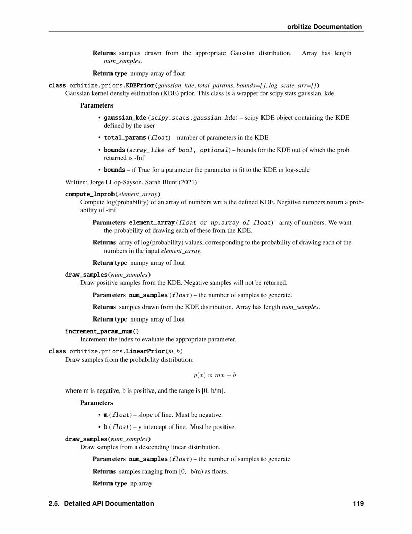
orbitize Documentation
Returns samples drawn from the appropriate Gaussian distribution. Array has lengthnum_samples.
Return type numpy array of float
class orbitize.priors.KDEPrior(gaussian_kde, total_params, bounds=[], log_scale_arr=[])Gaussian kernel density estimation (KDE) prior. This class is a wrapper for scipy.stats.gaussian_kde.
Parameters
• gaussian_kde (scipy.stats.gaussian_kde) – scipy KDE object containing the KDEdefined by the user
• total_params (float) – number of parameters in the KDE
• bounds (array_like of bool, optional) – bounds for the KDE out of which the probreturned is -Inf
• bounds – if True for a parameter the parameter is fit to the KDE in log-scale
Written: Jorge LLop-Sayson, Sarah Blunt (2021)
compute_lnprob(element_array)Compute log(probability) of an array of numbers wrt a the defined KDE. Negative numbers return a prob-ability of -inf.
Parameters element_array (float or np.array of float) – array of numbers. We wantthe probability of drawing each of these from the KDE.
Returns array of log(probability) values, corresponding to the probability of drawing each of thenumbers in the input element_array.
Return type numpy array of float
draw_samples(num_samples)Draw positive samples from the KDE. Negative samples will not be returned.
Parameters num_samples (float) – the number of samples to generate.
Returns samples drawn from the KDE distribution. Array has length num_samples.
Return type numpy array of float
increment_param_num()Increment the index to evaluate the appropriate parameter.
class orbitize.priors.LinearPrior(m, b)Draw samples from the probability distribution:
𝑝(𝑥) ∝ 𝑚𝑥 + 𝑏
where m is negative, b is positive, and the range is [0,-b/m].
Parameters
• m (float) – slope of line. Must be negative.
• b (float) – y intercept of line. Must be positive.
draw_samples(num_samples)Draw samples from a descending linear distribution.
Parameters num_samples (float) – the number of samples to generate
Returns samples ranging from [0, -b/m) as floats.
Return type np.array
2.5. Detailed API Documentation 119

orbitize Documentation
class orbitize.priors.LogUniformPrior(minval, maxval)This is the probability distribution 𝑝(𝑥) ∝ 1/𝑥
The __init__ method should take in a “min” and “max” value of the distribution, which correspond to the domainof the prior. (If this is not implemented, the prior has a singularity at 0 and infinite integrated probability).
Parameters
• minval (float) – the lower bound of this distribution
• maxval (float) – the upper bound of this distribution
compute_lnprob(element_array)Compute the prior probability of each element given that its drawn from a Log-Uniofrm prior
Parameters element_array (float or np.array of float) – array of paramters to com-pute the prior probability of
Returns array of prior probabilities
Return type np.array
draw_samples(num_samples)Draw samples from this 1/x distribution.
Parameters num_samples (float) – the number of samples to generate
Returns samples ranging from [minval, maxval) as floats.
Return type np.array
class orbitize.priors.NearestNDInterpPrior(interp_fct, total_params)Nearest Neighbor interp. This class is a wrapper for scipy.interpolate.NearestNDInterpolator.
Parameters
• interp_fct (scipy.interpolate.NearestNDInterpolator) – scipy Interpolator ob-ject containing the NDInterpolator defined by the user
• total_params (float) – number of parameters
Written: Jorge LLop-Sayson (2021)
compute_lnprob(element_array)Compute log(probability) of an array of numbers wrt a the defined ND interpolator. Negative numbersreturn a probability of -inf.
Parameters element_array (float or np.array of float) – array of numbers. We wantthe probability of drawing each of these from the ND interpolator.
Returns array of log(probability) values, corresponding to the probability of drawing each of thenumbers in the input element_array.
Return type numpy array of float
draw_samples(num_samples)Draw positive samples from the ND interpolator. Negative samples will not be returned.
Parameters num_samples (float) – the number of samples to generate.
Returns samples drawn from the ND interpolator distribution. Array has length num_samples.
Return type numpy array of float
increment_param_num()Increment the index to evaluate the appropriate parameter.
120 Chapter 2. User Guide:
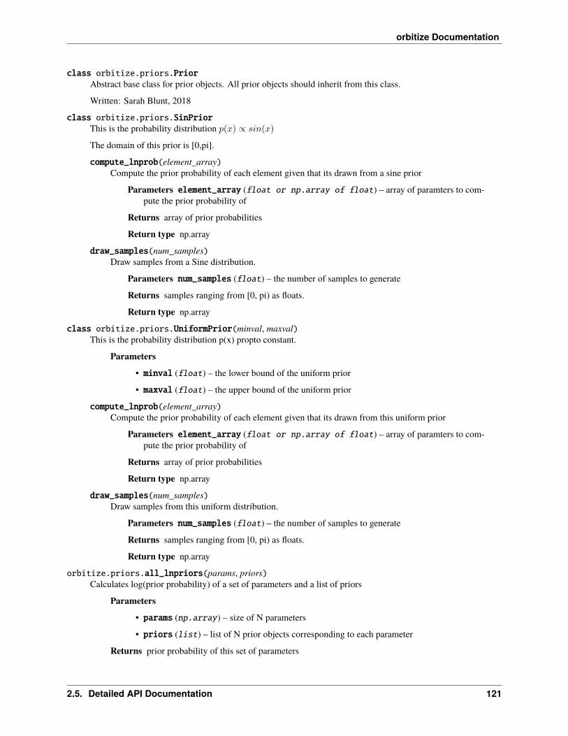
orbitize Documentation
class orbitize.priors.PriorAbstract base class for prior objects. All prior objects should inherit from this class.
Written: Sarah Blunt, 2018
class orbitize.priors.SinPriorThis is the probability distribution 𝑝(𝑥) ∝ 𝑠𝑖𝑛(𝑥)
The domain of this prior is [0,pi].
compute_lnprob(element_array)Compute the prior probability of each element given that its drawn from a sine prior
Parameters element_array (float or np.array of float) – array of paramters to com-pute the prior probability of
Returns array of prior probabilities
Return type np.array
draw_samples(num_samples)Draw samples from a Sine distribution.
Parameters num_samples (float) – the number of samples to generate
Returns samples ranging from [0, pi) as floats.
Return type np.array
class orbitize.priors.UniformPrior(minval, maxval)This is the probability distribution p(x) propto constant.
Parameters
• minval (float) – the lower bound of the uniform prior
• maxval (float) – the upper bound of the uniform prior
compute_lnprob(element_array)Compute the prior probability of each element given that its drawn from this uniform prior
Parameters element_array (float or np.array of float) – array of paramters to com-pute the prior probability of
Returns array of prior probabilities
Return type np.array
draw_samples(num_samples)Draw samples from this uniform distribution.
Parameters num_samples (float) – the number of samples to generate
Returns samples ranging from [0, pi) as floats.
Return type np.array
orbitize.priors.all_lnpriors(params, priors)Calculates log(prior probability) of a set of parameters and a list of priors
Parameters
• params (np.array) – size of N parameters
• priors (list) – list of N prior objects corresponding to each parameter
Returns prior probability of this set of parameters
2.5. Detailed API Documentation 121
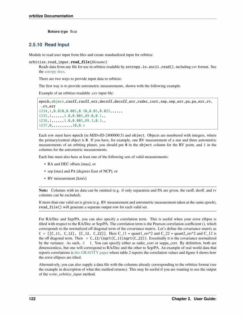
orbitize Documentation
Return type float
2.5.10 Read Input
Module to read user input from files and create standardized input for orbitize
orbitize.read_input.read_file(filename)Reads data from any file for use in orbitize readable by astropy.io.ascii.read(), including csv format. Seethe astropy docs.
There are two ways to provide input data to orbitize.
The first way is to provide astrometric measurements, shown with the following example.
Example of an orbitize-readable .csv input file:
epoch,object,raoff,raoff_err,decoff,decoff_err,radec_corr,sep,sep_err,pa,pa_err,rv,→˓rv_err1234,1,0.010,0.005,0.50,0.05,0.025,,,,,,1235,1,,,,,,1.0,0.005,89.0,0.1,,1236,1,,,,,,1.0,0.005,89.3,0.3,,1237,0,,,,,,,,,,10,0.1
Each row must have epoch (in MJD=JD-2400000.5) and object. Objects are numbered with integers, wherethe primary/central object is 0. If you have, for example, one RV measurement of a star and three astrometricmeasurements of an orbiting planet, you should put 0 in the object column for the RV point, and 1 in thecolumns for the astrometric measurements.
Each line must also have at least one of the following sets of valid measurements:
• RA and DEC offsets [mas], or
• sep [mas] and PA [degrees East of NCP], or
• RV measurement [km/s]
Note: Columns with no data can be omitted (e.g. if only separation and PA are given, the raoff, deoff, and rvcolumns can be excluded).
If more than one valid set is given (e.g. RV measurement and astrometric measurement taken at the same epoch),read_file() will generate a separate output row for each valid set.
For RA/Dec and Sep/PA, you can also specify a correlation term. This is useful when your error ellipse istilted with respect to the RA/Dec or Sep/PA. The correlation term is the Pearson correlation coefficient (), whichcorresponds to the normalized off diagonal term of the covariance matrix. Let’s define the covariance matrix asC = [[C_11, C_12], [C_12, C_22]]. Here C_11 = quant1_err^2 and C_22 = quant2_err^2 and C_12 isthe off diagonal term. Then = C_12/(sqrt(C_11)sqrt(C_22)). Essentially it is the covariance normalizedby the variance. As such, -1 1. You can specify either as radec_corr or seppa_corr. By definition, both aredimensionless, but one will correspond to RA/Dec and the other to Sep/PA. An example of real world data thatreports correlations is this GRAVITY paper where table 2 reports the correlation values and figure 4 shows howthe error ellipses are tilted.
Alternatively, you can also supply a data file with the columns already corresponding to the orbitize format (seethe example in description of what this method returns). This may be useful if you are wanting to use the outputof the write_orbitize_input method.
122 Chapter 2. User Guide:
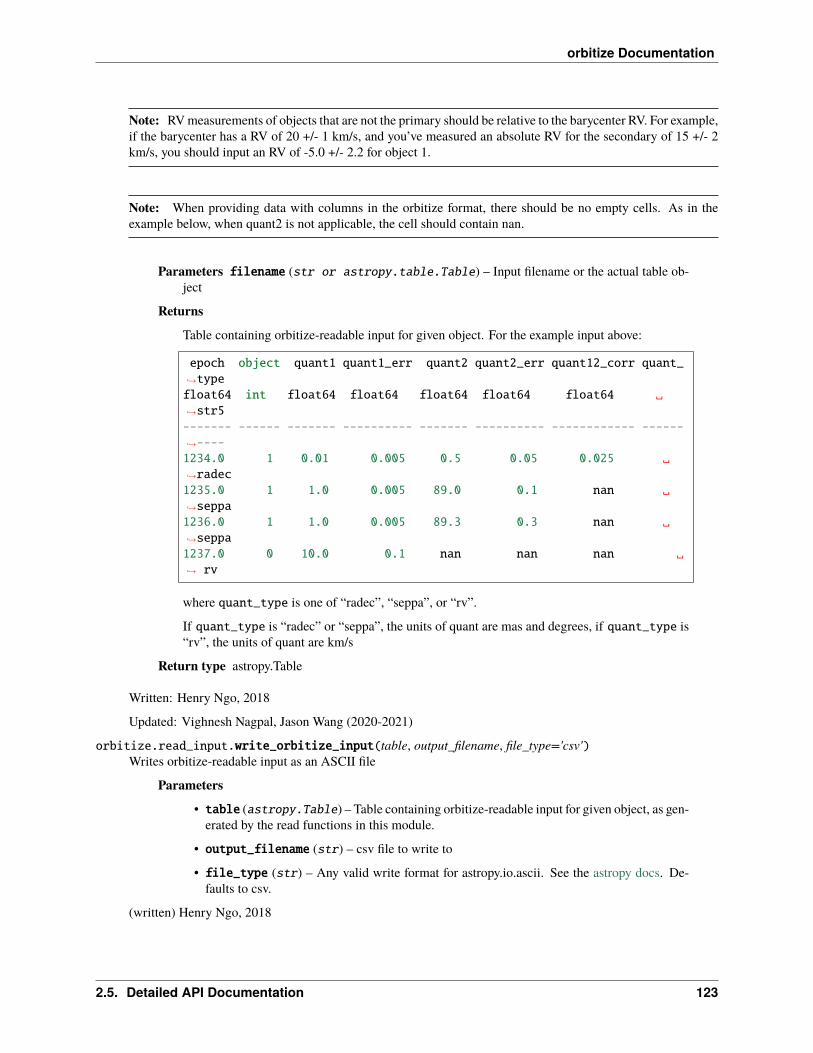
orbitize Documentation
Note: RV measurements of objects that are not the primary should be relative to the barycenter RV. For example,if the barycenter has a RV of 20 +/- 1 km/s, and you’ve measured an absolute RV for the secondary of 15 +/- 2km/s, you should input an RV of -5.0 +/- 2.2 for object 1.
Note: When providing data with columns in the orbitize format, there should be no empty cells. As in theexample below, when quant2 is not applicable, the cell should contain nan.
Parameters filename (str or astropy.table.Table) – Input filename or the actual table ob-ject
Returns
Table containing orbitize-readable input for given object. For the example input above:
epoch object quant1 quant1_err quant2 quant2_err quant12_corr quant_→˓typefloat64 int float64 float64 float64 float64 float64 →˓str5------- ------ ------- ---------- ------- ---------- ------------ ------→˓----1234.0 1 0.01 0.005 0.5 0.05 0.025 →˓radec1235.0 1 1.0 0.005 89.0 0.1 nan →˓seppa1236.0 1 1.0 0.005 89.3 0.3 nan →˓seppa1237.0 0 10.0 0.1 nan nan nan →˓ rv
where quant_type is one of “radec”, “seppa”, or “rv”.
If quant_type is “radec” or “seppa”, the units of quant are mas and degrees, if quant_type is“rv”, the units of quant are km/s
Return type astropy.Table
Written: Henry Ngo, 2018
Updated: Vighnesh Nagpal, Jason Wang (2020-2021)
orbitize.read_input.write_orbitize_input(table, output_filename, file_type='csv')Writes orbitize-readable input as an ASCII file
Parameters
• table (astropy.Table) – Table containing orbitize-readable input for given object, as gen-erated by the read functions in this module.
• output_filename (str) – csv file to write to
• file_type (str) – Any valid write format for astropy.io.ascii. See the astropy docs. De-faults to csv.
(written) Henry Ngo, 2018
2.5. Detailed API Documentation 123
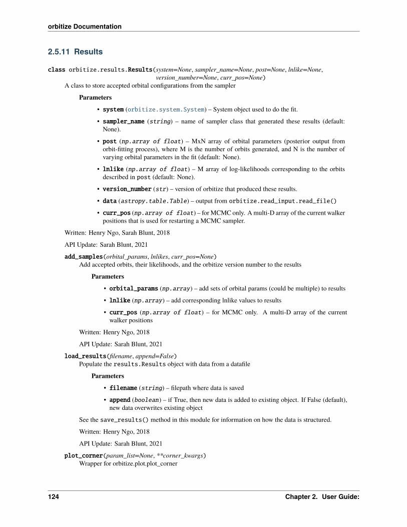
orbitize Documentation
2.5.11 Results
class orbitize.results.Results(system=None, sampler_name=None, post=None, lnlike=None,version_number=None, curr_pos=None)
A class to store accepted orbital configurations from the sampler
Parameters
• system (orbitize.system.System) – System object used to do the fit.
• sampler_name (string) – name of sampler class that generated these results (default:None).
• post (np.array of float) – MxN array of orbital parameters (posterior output fromorbit-fitting process), where M is the number of orbits generated, and N is the number ofvarying orbital parameters in the fit (default: None).
• lnlike (np.array of float) – M array of log-likelihoods corresponding to the orbitsdescribed in post (default: None).
• version_number (str) – version of orbitize that produced these results.
• data (astropy.table.Table) – output from orbitize.read_input.read_file()
• curr_pos (np.array of float) – for MCMC only. A multi-D array of the current walkerpositions that is used for restarting a MCMC sampler.
Written: Henry Ngo, Sarah Blunt, 2018
API Update: Sarah Blunt, 2021
add_samples(orbital_params, lnlikes, curr_pos=None)Add accepted orbits, their likelihoods, and the orbitize version number to the results
Parameters
• orbital_params (np.array) – add sets of orbital params (could be multiple) to results
• lnlike (np.array) – add corresponding lnlike values to results
• curr_pos (np.array of float) – for MCMC only. A multi-D array of the currentwalker positions
Written: Henry Ngo, 2018
API Update: Sarah Blunt, 2021
load_results(filename, append=False)Populate the results.Results object with data from a datafile
Parameters
• filename (string) – filepath where data is saved
• append (boolean) – if True, then new data is added to existing object. If False (default),new data overwrites existing object
See the save_results() method in this module for information on how the data is structured.
Written: Henry Ngo, 2018
API Update: Sarah Blunt, 2021
plot_corner(param_list=None, **corner_kwargs)Wrapper for orbitize.plot.plot_corner
124 Chapter 2. User Guide:
orbitize Documentation
plot_orbits(object_to_plot=1, start_mjd=51544.0, num_orbits_to_plot=100, num_epochs_to_plot=100,square_plot=True, show_colorbar=True,cmap=<matplotlib.colors.LinearSegmentedColormap object>, sep_pa_color='lightgrey',sep_pa_end_year=2025.0, cbar_param='Epoch [year]', mod180=False,rv_time_series=False, plot_astrometry=True, plot_astrometry_insts=False, fig=None)
Wrapper for orbitize.plot.plot_orbits
print_results()Prints median and 68% credible intervals alongside fitting labels
save_results(filename)Save results.Results object to an hdf5 file
Parameters filename (string) – filepath to save to
Save attributes from the results.Results object.
sampler_name, tau_ref_epcoh, version_number are attributes of the root group. post, lnlike, andparameter_labels are datasets that are members of the root group.
Written: Henry Ngo, 2018
API Update: Sarah Blunt, 2021
2.5.12 Sampler
class orbitize.sampler.MCMC(system, num_temps=20, num_walkers=1000, num_threads=1,like='chi2_lnlike', custom_lnlike=None, prev_result_filename=None)
MCMC sampler. Supports either parallel tempering or just regular MCMC. Parallel tempering will be run ifnum_temps > 1 Parallel-Tempered MCMC Sampler uses ptemcee, a fork of the emcee Affine-infariant samplerAffine-Invariant Ensemble MCMC Sampler uses emcee.
Warning: may not work well for multi-modal distributions
Parameters
• system (system.System) – system.System object
• num_temps (int) – number of temperatures to run the sampler at. Parallel tempering willbe used if num_temps > 1 (default=20)
• num_walkers (int) – number of walkers at each temperature (default=1000)
• num_threads (int) – number of threads to use for parallelization (default=1)
• like (str) – name of likelihood function in lnlike.py
• custom_lnlike (func) – ability to include an addition custom likelihood function in the fit.The function looks like clnlikes = custon_lnlike(params) where params is a RxMarray of fitting parameters, where R is the number of orbital paramters (can be passed insystem.compute_model()), and M is the number of orbits we need model predictions for. Itreturns clnlikes which is an array of length M, or it can be a single float if M = 1.
• prev_result_filename (str) – if passed a filename to an HDF5 file containing a or-bitize.Result data, MCMC will restart from where it left off.
Written: Jason Wang, Henry Ngo, 2018
2.5. Detailed API Documentation 125
orbitize Documentation
check_prior_support()Review the positions of all MCMC walkers, to verify that they are supported by the prior space. Thisfunction will raise a descriptive ValueError if any positions lie outside prior support. Otherwise, it willreturn nothing.
(written): Adam Smith, 2021
chop_chains(burn, trim=0)Permanently removes steps from beginning (and/or end) of chains from the Results object. Also updatescurr_pos if steps are removed from the end of the chain.
Parameters
• burn (int) – The number of steps to remove from the beginning of the chains
• trim (int) – The number of steps to remove from the end of the chians (optional)
Warning: Does not update bookkeeping arrays within MCMC sampler object.
(written): Henry Ngo, 2019
examine_chains(param_list=None, walker_list=None, n_walkers=None, step_range=None,transparency=1)
Plots position of walkers at each step from Results object. Returns list of figures, one per parameter :paramparam_list: List of strings of parameters to plot (e.g. “sma1”)
If None (default), all parameters are plotted
Parameters
• walker_list – List or array of walker numbers to plot If None (default), all walkers areplotted
• n_walkers (int) – Randomly select n_walkers to plot Overrides walker_list if this is setIf None (default), walkers selected as per walker_list
• step_range (array or tuple) – Start and end values of step numbers to plot If None(default), all the steps are plotted
• transparency (int or float) – Determines visibility of the plotted function If 1 (de-fault) results plot at 100% opacity
Returns Walker position plot for each parameter selected
Return type List of matplotlib.pyplot.Figure objects
(written): Henry Ngo, 2019
run_sampler(total_orbits, burn_steps=0, thin=1, examine_chains=False, output_filename=None,periodic_save_freq=None)
Runs PT MCMC sampler. Results are stored in self.chain and self.lnlikes. Results also added toorbitize.results.Results object (self.results)
Note: Can be run multiple times if you want to pause and inspect things. Each call will continue from theend state of the last execution.
Parameters
126 Chapter 2. User Guide:

orbitize Documentation
• total_orbits (int) – total number of accepted possible orbits that are desired. Thisequals num_steps_per_walker x num_walkers
• burn_steps (int) – optional paramter to tell sampler to discard certain number of stepsat the beginning
• thin (int) – factor to thin the steps of each walker by to remove correlations in the walkersteps
• examine_chains (boolean) – Displays plots of walkers at each step by running exam-ine_chains after total_orbits sampled.
• output_filename (str) – Optional filepath for where results file can be saved.
• periodic_save_freq (int) – Optionally, save the current results intooutput_filename every nth step while running, where n is value passed into thisvariable.
Returns the sampler used to run the MCMC
Return type emcee.sampler object
validate_xyz_positions()If using the XYZ basis, walkers might be initialized in an invalid region of parameter space. This functionfixes that by replacing invalid positions by new randomly generated positions until all are valid.
class orbitize.sampler.OFTI(system, like='chi2_lnlike', custom_lnlike=None)OFTI Sampler
Parameters
• system (system.System) – system.System object
• like (string) – name of likelihood function in lnlike.py
• custom_lnlike (func) – ability to include an addition custom likelihood function in the fit.The function looks like clnlikes = custon_lnlike(params) where params is a RxMarray of fitting parameters, where R is the number of orbital paramters (can be passed insystem.compute_model()), and M is the number of orbits we need model predictions for. Itreturns clnlikes which is an array of length M, or it can be a single float if M = 1.
Written: Isabel Angelo, Sarah Blunt, Logan Pearce, 2018
prepare_samples(num_samples)Prepare some orbits for rejection sampling. This draws random orbits from priors, and performs scale &rotate.
Parameters num_samples (int) – number of orbits to draw and scale & rotate for OFTI to runrejection sampling on
Returns array of prepared samples. The first dimension has size of num_samples. This shouldbe passed into OFTI.reject()
Return type np.array
reject(samples)Runs rejection sampling on some prepared samples.
Parameters samples (np.array) – array of prepared samples. The first dimension has sizenum_samples. This should be the output of prepare_samples().
Returns
np.array: a subset of samples that are accepted based on the data.
2.5. Detailed API Documentation 127

orbitize Documentation
np.array: the log likelihood values of the accepted orbits.
Return type tuple
run_sampler(total_orbits, num_samples=10000, num_cores=None)Runs OFTI in parallel on multiple cores until we get the number of total accepted orbits we want.
Parameters
• total_orbits (int) – total number of accepted orbits desired by user
• num_samples (int) – number of orbits to prepare for OFTI to run rejection sampling on.Defaults to 10000.
• num_cores (int) – the number of cores to run OFTI on. Defaults to number of coresavailabe.
Returns array of accepted orbits. Size: total_orbits.
Return type np.array
Written by: Vighnesh Nagpal(2019)
class orbitize.sampler.Sampler(system, like='chi2_lnlike', custom_lnlike=None)Abstract base class for sampler objects. All sampler objects should inherit from this class.
Written: Sarah Blunt, 2018
2.5.13 System
class orbitize.system.System(num_secondary_bodies, data_table, stellar_or_system_mass, plx, mass_err=0,plx_err=0, restrict_angle_ranges=False, tau_ref_epoch=58849,fit_secondary_mass=False, hipparcos_IAD=None, gaia=None,fitting_basis='Standard', use_rebound=False)
A class to store information about a system (data & priors) and calculate model predictions given a set of orbitalparameters.
Parameters
• num_secondary_bodies (int) – number of secondary bodies in the system. Should be atleast 1.
• data_table (astropy.table.Table) – output from orbitize.read_input.read_file()
• stellar_or_system_mass (float) – mass of the primary star (if fitting for dynamicalmasses of both components) or total system mass (if fitting using relative astrometry only)[M_sol]
• plx (float) – mean parallax of the system, in mas
• mass_err (float, optional) – uncertainty on stellar_or_system_mass, in M_sol
• plx_err (float, optional) – uncertainty on plx, in mas
• restrict_angle_ranges (bool, optional) – if True, restrict the ranges of the positionangle of nodes to [0,180) to get rid of symmetric double-peaks for imaging-only datasets.
• tau_ref_epoch (float, optional) – reference epoch for defining tau (MJD). Default is58849 (Jan 1, 2020).
128 Chapter 2. User Guide:
orbitize Documentation
• fit_secondary_mass (bool, optional) – if True, include the dynamical mass of theorbiting body as a fitted parameter. If this is set to False, stellar_or_system_mass istaken to be the total mass of the system. (default: False)
• hipparcos_IAD (orbitize.hipparcos.HipparcosLogProb) – an object containing in-formation & precomputed values relevant to Hipparcos IAD fitting. See hipparcos.py formore details.
• gaia (orbitize.gaia.GaiaLogProb) – an object containing information & precomputedvalues relevant to Gaia astrometrry fitting. See gaia.py for more details.
• fitting_basis (str) – the name of the class corresponding to the fitting basis to be used.See basis.py for a list of implemented fitting bases.
• use_rebound (bool) – if True, use an n-body backend solver instead of a Keplerian solver.
Priors are initialized as a list of orbitize.priors.Prior objects and stored in the variable System.sys_priors. Youshould initialize this class, then overwrite priors you wish to customize. You can use the System.param_idxattribute to figure out which indices correspond to which fitting parameters. See the “changing priors” tutorialfor more detail.
Written: Sarah Blunt, Henry Ngo, Jason Wang, 2018
compute_all_orbits(params_arr, epochs=None, comp_rebound=False)Calls orbitize.kepler.calc_orbit and optionally accounts for multi-body interactions. Also computes totalquantities like RV (without jitter/gamma)
Parameters
• params_arr (np.array of float) – RxM array of fitting parameters, where R is thenumber of parameters being fit, and M is the number of orbits we need model predictionsfor. Must be in the same order documented in System() above. If M=1, this can be a 1darray.
• epochs (np.array of float) – epochs (in mjd) at which to compute orbit predictions.
• comp_rebound (bool, optional) – A secondary optional input for use of N-body solverRebound; by default, this will be set to false and a Kepler solver will be used instead.
Returns
raoff (np.array of float): N_epochs x N_bodies x N_orbits array of RA offsets frombarycenter at each epoch.
decoff (np.array of float): N_epochs x N_bodies x N_orbits array of Dec offsets frombarycenter at each epoch.
vz (np.array of float): N_epochs x N_bodies x N_orbits array of radial velocities at eachepoch.
Return type tuple
compute_model(params_arr, use_rebound=False)Compute model predictions for an array of fitting parameters. Calls the above compute_all_orbits() func-tion, adds jitter/gamma to RV measurements, and propagates these predictions to a model array that can besubtracted from a data array to compute chi2.
Parameters
• params_arr (np.array of float) – RxM array of fitting parameters, where R is thenumber of parameters being fit, and M is the number of orbits we need model predictionsfor. Must be in the same order documented in System() above. If M=1, this can be a 1darray.
2.5. Detailed API Documentation 129
orbitize Documentation
• use_rebound (bool, optional) – A secondary optional input for use of N-body solverRebound; by default, this will be set to false and a Kepler solver will be used instead.
Returns
np.array of float: Nobsx2xM array model predictions. If M=1, this is a 2d array, other-wise it is a 3d array.
np.array of float: Nobsx2xM array jitter predictions. If M=1, this is a 2d array, other-wise it is a 3d array.
Return type tuple of
convert_data_table_radec2seppa(body_num=1)Converts rows of self.data_table given in radec to seppa. Note that self.input_table remains unchanged.
Parameters body_num (int) – which object to convert (1 = first planet)
save(hf )Saves the current object to an hdf5 file
Parameters hf (h5py._hl.files.File) – a currently open hdf5 file in which to save the ob-ject.
orbitize.system.radec2seppa(ra, dec, mod180=False)Convenience function for converting from right ascension/declination to separation/ position angle.
Parameters
• ra (np.array of float) – array of RA values, in mas
• dec (np.array of float) – array of Dec values, in mas
• mod180 (Bool) – if True, output PA values will be given in range [180, 540) (useful forplotting short arcs with PAs that cross 360 during observations) (default: False)
Returns (separation [mas], position angle [deg])
Return type tuple of float
orbitize.system.seppa2radec(sep, pa)Convenience function to convert sep/pa to ra/dec
Parameters
• sep (np.array of float) – array of separation in mas
• pa (np.array of float) – array of position angles in degrees
Returns (ra [mas], dec [mas])
Return type tuple
orbitize.system.transform_errors(x1, x2, x1_err, x2_err, x12_corr, transform_func, nsamps=100000)
Transform errors and covariances from one basis to another using a Monte Carlo apporach
Parameters
• x1 (float) – planet location in first coordinate (e.g., RA, sep) before transformation
• x2 (float) – planet location in the second coordinate (e.g., Dec, PA) before transformation)
• x1_err (float) – error in x1
• x2_err (float) – error in x2
130 Chapter 2. User Guide:
orbitize Documentation
• x12_corr (float) – correlation between x1 and x2
• transform_func (function) – function that transforms between (x1, x2) and (x1p, x2p)(the transformed coordinates). The function signature should look like: x1p, x2p = trans-form_func(x1, x2)
• nsamps – number of samples to draw more the Monte Carlo approach. More is slower butmore accurate.
2.5. Detailed API Documentation 131

orbitize Documentation
132 Chapter 2. User Guide:
CHAPTER
THREE
CHANGELOG:
2.0.0 (2021-10-13)
This is the official release of orbitize! version 2.
Big changes:
• Fit Gaia positions (@sblunt)
• New plotting module & API (@sblunt)
• Relative planet RVs now officially supported & tested (@sblunt)
• GPU Kepler solver (@devincody)
• RV end-to-end test added (@vighnesh-nagpal)
Small changes:
• Hipparcos calculation bugfix (@sblunt)
• v1 results backwards compatibility bugfix (@sblunt)
• windows install docs update (@sblunt
• basis bugfix with new API (@TirthDS, @sblunt)
• handle Hipparcos 2021 data format (@sblunt)
• clarify API on mtot/mstar (@lhirsch238, @sblunt)
2.0b1 (2021-09-03)
This is the beta release of orbitize! version 2.
Big changes:
• N-body Kepler solver backend! (@sofiacovarrubias)
• Fitting in XYZ orbital basis! (@rferrerc)
• API for fitting in arbitrary new orbital bases! (@TirthDS)
• compute_all_orbits separated out, streamlining stellar astrometry & RV calculations (@sblunt)
• Hip IAD! (@sblunt)
• param_idx now used everywhere under the hood (system parsing updated) (@sblunt)
• KDE prior added (inspiration=training on RV fits) (@jorgellop)
Small changes:
• HD 4747 rv data file fix for the RV tutorial (@lhirsch238)
133

orbitize Documentation
• Add check_prior_support to sampler.MCMC (@adj-smith)
• Update example generation code in MCMC v OFTI tutorial (@semaphoreP)
• Fixed plotting bug (issue #243) (@TirthDS)
• Expand FAQ section (@semaphoreP)
• use astropy tables in results (@semaphoreP)
• Expand converge section of MCMC tutorial (@semaphoreP)
• Deprecated functions and deprecation warnings officially removed (@semaphoreP)
• Fix logic in setting of track_planet_perturbs (@sblunt)
• Fix plotting error if orbital periods are > 1e9 days (@sblunt)
• Add method for printing results of a fit (@sblunt)
1.16.1 (2021-06-27)
• Fixed chop_chains() function to copy original data over when updating Results object (@TirthDS)
1.16.0 (2021-06-23)
• User-defined prior on PAN were not being applied if OFTI is used; fixed (@sblunt)
• Dates in HD 4747 data file were incorrect; fixed (@lhirsch238)
1.15.5 (2021-07-20)
• Addressed issue #177, giving Results and Sampler classes a parameter label array (@sblunt)
• Fixed a bug that was causing RA/Dec data points to display wrong in orbit plots (@sblunt)
1.15.4 (2021-06-18)
• Bugfix for issue #234 (@semaphoreP, @adj-smith)
1.15.3 (2021-06-07)
• Add codeastro mode to pytest that prints out a SECRET CODE if tests pass omgomg (@semaphoreP)
1.15.2 (2021-05-11)
• Fixed backwards-compatibility bug with version numbers and saving/loading (@semaphoreP, @wbalmer)
1.15.1 (2021-03-29)
• Fixed bug where users with Results objects from v<14.0 couldn’t load using v>=14.0 (@semaphoreP, @wbalmer)
• Fixed order of Axes objects in Advanced Plotting tutorial (@wbalmer, @sblunt)
1.15.0 (2021-02-23)
• Handle covariances in input astrometry (@semaphoreP)
1.14.0 (2021-02-12)
• Version number now saved in results object (@hgallamore)
• Joint RV+astrometry fits can now handle different RV instruments! (@vighnesh-nagpal,@Rob685, @lhirsch238)
• New “FAQ” section added to docs (@semaphoreP)
• Bugfix for multiplanet code (@semaphoreP) introduced in PR #192
• now you can pass a preexisting Figure object into results.plot_orbit (@sblunt)
134 Chapter 3. Changelog:
orbitize Documentation
• colorbar label is now “Epoch [year]” (@sblunt)
• corner plot maker can now handle fixed parameters without crashing (@sblunt)
1.13.1 (2021-01-25)
• compute_sep in radvel_utils submodule now returns mp (@sblunt)
• astropy._erfa was deprecated (now in separate package). Dependencies updated. (@sblunt)
1.13.0 (2020-11-8)
• Added radvel-utils submodule which allows users to calculate projected separation posteriors given RadVelchains (@sblunt)
• Fixed a total mass/primary mass mixup bug that was causing problems for equal-mass binary RV+astrometryjoint fits (@sblunt)
• Bugfix for multiplanet perturbation approximation: now only account for inner planets only when computingperturbations (@semaphoreP)
1.12.1 (2020-9-6)
• tau_ref_epoch is now set to Jan 1, 2020 throughout the code (@semaphoreP)
• restrict_angle_ranges keyword now works as expected for OFTI (@sblunt)
1.12.0 (2020-8-28)
• Compatibility with emcee>=3 (@sblunt)
1.11.3 (2020-8-20)
• Save results section of OFTI tutorial now current (@rferrerc)
• Modifying MCMC initial positions tutorial documentation now uses correct orbital elements (@rferrerc)
1.11.2 (2020-8-10)
• Added transparency option for plotting MCMC chains (@sofiacovarrubias)
• Removed some redundant code (@MissingBrainException)
1.11.1 (2020-6-11)
• Fixed a string formatting bug causing corner plots to fail for RV+astrometry fits
1.11.0 (2020-4-14)
• Multiplanet support!
• Changes to directory structure of sample data files
• Fixed a bug that was causing corner plots to fail on loaded results objects
1.10.0 (2020-3-6)
• Joint RV + relative astrometry fitting capabilities!
• New tutorial added
1.9.0 (2020-1-24)
• Require astropy>=4
• Minor documentation upgrades
• This is the first Python 2 noncompliant version
1.8.0 (2020-1-24)
135
orbitize Documentation
• Bugfixes related to numpy and astropy upgrades
• This is the last version that will support Python 2
1.7.0 (2019-11-10)
• Default corner plots now display angles in degrees instead of radians
• Add a keyword for plotting orbits that cross PA=360
1.6.0 (2019-10-1)
• Mikkola solver now implemented in C-Kepler solver
• Fixed a bug with parallel processing for OFTI
• Added orbit vizualisation jupyter nb show-me-the-orbit to docs/tutorials
• New methods for viewing/chopping MCMC chains
• Require emcee<3 for now
1.5.0 (2019-9-9)
• Parallel processing for OFTI.
• Fixed a bug converting errors in RA/Dec to sep/PA in OFTI.
• OFTI and MCMC now both return likelihood, whereas before one returned posterior.
• Updated logic for restricting Omega and omega bounds.
1.4.0 (2019-7-15)
• API change to lay the groundwork for dynamical mass calculation.
• JeffreysPrior -> LogUniformPrior
• New tutorials.
• Added some informative error messages for input tables.
• Bugfixes.
1.3.1 (2019-6-19)
• Bugfix for RA/Dec inputs to the OFTI sampler (Issue #108).
1.3.0 (2019-6-4)
• Add ability to customize date of tau definition.
• Sampler now saves choice of tau reference with results.
• Default tau value is now Jan 1, 2020.
• Small bugfixes.
1.2.0 (2019-3-21)
• Remove unnecessary astropy date warnings.
• Add custom likelihood function.
• Add progress bar for ptemcee sampler.
• Add customizable color axis for orbit plots.
• Small bugfixes.
1.1.0 (2019-1-6)
136 Chapter 3. Changelog:

orbitize Documentation
• Add sep/PA panels to orbit plot.
• GaussianPrior now operates on only positive numbers by default.
1.0.2 (2018-12-4)
• Expand input reading functionality.
• Bugfixes for MCMC.
1.0.1 (2018-11-20)
• Bugfix for building on CentOS machines.
1.0.0 (2018-10-30)
• Initial release.
137

orbitize Documentation
138 Chapter 3. Changelog:
PYTHON MODULE INDEX
oorbitize, 128orbitize.basis, 101orbitize.driver, 110orbitize.gaia, 111orbitize.hipparcos, 112orbitize.kepler, 113orbitize.lnlike, 115orbitize.nbody, 116orbitize.plot, 116orbitize.priors, 118orbitize.read_input, 122orbitize.results, 124orbitize.sampler, 125orbitize.system, 128
139

orbitize Documentation
140 Python Module Index
INDEX
Aadd_samples() (orbitize.results.Results method), 124all_lnpriors() (in module orbitize.priors), 121
BBasis (class in orbitize.basis), 101
Ccalc_orbit() (in module orbitize.kepler), 113calc_orbit() (in module orbitize.nbody), 116check_prior_support() (orbitize.sampler.MCMC
method), 125chi2_lnlike() (in module orbitize.lnlike), 115chi2_norm_term() (in module orbitize.lnlike), 115chop_chains() (orbitize.sampler.MCMC method), 126compute_all_orbits() (orbitize.system.System
method), 129compute_companion_mass() (orbitize.basis.SemiAmp
method), 104compute_companion_sma() (orbitize.basis.SemiAmp
method), 104compute_lnlike() (orbitize.gaia.GaiaLogProb
method), 111compute_lnlike() (or-
bitize.hipparcos.HipparcosLogProb method),112
compute_lnprob() (orbitize.priors.GaussianPriormethod), 118
compute_lnprob() (orbitize.priors.KDEPrior method),119
compute_lnprob() (orbitize.priors.LogUniformPriormethod), 120
compute_lnprob() (or-bitize.priors.NearestNDInterpPrior method),120
compute_lnprob() (orbitize.priors.SinPrior method),121
compute_lnprob() (orbitize.priors.UniformPriormethod), 121
compute_model() (orbitize.system.System method), 129construct_priors() (orbitize.basis.Period method),
103
construct_priors() (orbitize.basis.SemiAmpmethod), 105
construct_priors() (orbitize.basis.Standard method),106
construct_priors() (orbitize.basis.XYZ method), 107convert_data_table_radec2seppa() (or-
bitize.system.System method), 130
Ddraw_samples() (orbitize.priors.GaussianPrior
method), 118draw_samples() (orbitize.priors.KDEPrior method),
119draw_samples() (orbitize.priors.LinearPrior method),
119draw_samples() (orbitize.priors.LogUniformPrior
method), 120draw_samples() (orbitize.priors.NearestNDInterpPrior
method), 120draw_samples() (orbitize.priors.SinPrior method), 121draw_samples() (orbitize.priors.UniformPrior
method), 121Driver (class in orbitize.driver), 110
Eexamine_chains() (orbitize.sampler.MCMC method),
126
Ffunc() (orbitize.basis.SemiAmp method), 105
GGaiaLogProb (class in orbitize.gaia), 111GaussianPrior (class in orbitize.priors), 118
HHipparcosLogProb (class in orbitize.hipparcos), 112
Iincrement_param_num() (orbitize.priors.KDEPrior
method), 119
141
orbitize Documentation
increment_param_num() (or-bitize.priors.NearestNDInterpPrior method),120
KKDEPrior (class in orbitize.priors), 119
LLinearPrior (class in orbitize.priors), 119load_results() (orbitize.results.Results method), 124LogUniformPrior (class in orbitize.priors), 120
MMCMC (class in orbitize.sampler), 125module
orbitize, 101, 110–113, 115, 116, 118, 122, 124,125, 128
orbitize.basis, 101orbitize.driver, 110orbitize.gaia, 111orbitize.hipparcos, 112orbitize.kepler, 113orbitize.lnlike, 115orbitize.nbody, 116orbitize.plot, 116orbitize.priors, 118orbitize.read_input, 122orbitize.results, 124orbitize.sampler, 125orbitize.system, 128
NNearestNDInterpPrior (class in orbitize.priors), 120nielsen_iad_refitting_test() (in module or-
bitize.hipparcos), 113
OOFTI (class in orbitize.sampler), 127orbitize
module, 101, 110–113, 115, 116, 118, 122, 124, 125,128
orbitize.basismodule, 101
orbitize.drivermodule, 110
orbitize.gaiamodule, 111
orbitize.hipparcosmodule, 112
orbitize.keplermodule, 113
orbitize.lnlikemodule, 115
orbitize.nbodymodule, 116
orbitize.plotmodule, 116
orbitize.priorsmodule, 118
orbitize.read_inputmodule, 122
orbitize.resultsmodule, 124
orbitize.samplermodule, 125
orbitize.systemmodule, 128
PPeriod (class in orbitize.basis), 102plot_corner() (in module orbitize.plot), 116plot_corner() (orbitize.results.Results method), 124plot_orbits() (in module orbitize.plot), 117plot_orbits() (orbitize.results.Results method), 124prepare_samples() (orbitize.sampler.OFTI method),
127print_results() (orbitize.results.Results method), 125Prior (class in orbitize.priors), 120
Rradec2seppa() (in module orbitize.system), 130read_file() (in module orbitize.read_input), 122reject() (orbitize.sampler.OFTI method), 127Results (class in orbitize.results), 124run_sampler() (orbitize.sampler.MCMC method), 126run_sampler() (orbitize.sampler.OFTI method), 128
SSampler (class in orbitize.sampler), 128save() (orbitize.system.System method), 130save_results() (orbitize.results.Results method), 125SemiAmp (class in orbitize.basis), 103seppa2radec() (in module orbitize.system), 130set_default_mass_priors() (orbitize.basis.Basis
method), 101set_hip_iad_priors() (orbitize.basis.Basis method),
102set_rv_priors() (orbitize.basis.Basis method), 102SinPrior (class in orbitize.priors), 121Standard (class in orbitize.basis), 106standard_to_xyz() (orbitize.basis.XYZ method), 108switch_tau_epoch() (in module orbitize.basis), 109System (class in orbitize.system), 128
Ttau_to_manom() (in module orbitize.basis), 109
142 Index
orbitize Documentation
tau_to_manom() (in module orbitize.kepler), 114tau_to_tp() (in module orbitize.basis), 109to_period_basis() (orbitize.basis.Period method),
103to_semi_amp_basis() (orbitize.basis.SemiAmp
method), 105to_standard_basis() (orbitize.basis.Period method),
103to_standard_basis() (orbitize.basis.SemiAmp
method), 105to_standard_basis() (orbitize.basis.Standard
method), 106to_standard_basis() (orbitize.basis.XYZ method),
108to_xyz_basis() (orbitize.basis.XYZ method), 108tp_to_tau() (in module orbitize.basis), 110transform_errors() (in module orbitize.system), 130
UUniformPrior (class in orbitize.priors), 121
Vvalidate_xyz_positions() (orbitize.sampler.MCMC
method), 127verify_params() (orbitize.basis.Basis method), 102verify_params() (orbitize.basis.SemiAmp method),
106verify_params() (orbitize.basis.XYZ method), 108
Wwrite_orbitize_input() (in module or-
bitize.read_input), 123
XXYZ (class in orbitize.basis), 107xyz_to_standard() (orbitize.basis.XYZ method), 108
Index 143