sas/stat 15.1 user’s guide · getting started: sim2d procedure f 9191 getting started: sim2d...
TRANSCRIPT
SAS/STAT® 15.1User’s GuideThe SIM2D Procedure

This document is an individual chapter from SAS/STAT® 15.1 User’s Guide.
The correct bibliographic citation for this manual is as follows: SAS Institute Inc. 2018. SAS/STAT® 15.1 User’s Guide. Cary, NC:SAS Institute Inc.
SAS/STAT® 15.1 User’s Guide
Copyright © 2018, SAS Institute Inc., Cary, NC, USA
All Rights Reserved. Produced in the United States of America.
For a hard-copy book: No part of this publication may be reproduced, stored in a retrieval system, or transmitted, in any form or byany means, electronic, mechanical, photocopying, or otherwise, without the prior written permission of the publisher, SAS InstituteInc.
For a web download or e-book: Your use of this publication shall be governed by the terms established by the vendor at the timeyou acquire this publication.
The scanning, uploading, and distribution of this book via the Internet or any other means without the permission of the publisher isillegal and punishable by law. Please purchase only authorized electronic editions and do not participate in or encourage electronicpiracy of copyrighted materials. Your support of others’ rights is appreciated.
U.S. Government License Rights; Restricted Rights: The Software and its documentation is commercial computer softwaredeveloped at private expense and is provided with RESTRICTED RIGHTS to the United States Government. Use, duplication, ordisclosure of the Software by the United States Government is subject to the license terms of this Agreement pursuant to, asapplicable, FAR 12.212, DFAR 227.7202-1(a), DFAR 227.7202-3(a), and DFAR 227.7202-4, and, to the extent required under U.S.federal law, the minimum restricted rights as set out in FAR 52.227-19 (DEC 2007). If FAR 52.227-19 is applicable, this provisionserves as notice under clause (c) thereof and no other notice is required to be affixed to the Software or documentation. TheGovernment’s rights in Software and documentation shall be only those set forth in this Agreement.
SAS Institute Inc., SAS Campus Drive, Cary, NC 27513-2414
November 2018
SAS® and all other SAS Institute Inc. product or service names are registered trademarks or trademarks of SAS Institute Inc. in theUSA and other countries. ® indicates USA registration.
Other brand and product names are trademarks of their respective companies.
SAS software may be provided with certain third-party software, including but not limited to open-source software, which islicensed under its applicable third-party software license agreement. For license information about third-party software distributedwith SAS software, refer to http://support.sas.com/thirdpartylicenses.

Chapter 109
The SIM2D Procedure
ContentsOverview: SIM2D Procedure . . . . . . . . . . . . . . . . . . . . . . . . . . . . . . . . . . 9190
Introduction to Spatial Simulation . . . . . . . . . . . . . . . . . . . . . . . . . . . . 9190Getting Started: SIM2D Procedure . . . . . . . . . . . . . . . . . . . . . . . . . . . . . . . 9191
Preliminary Spatial Data Analysis . . . . . . . . . . . . . . . . . . . . . . . . . . . . 9191Investigating Variability by Simulation . . . . . . . . . . . . . . . . . . . . . . . . . 9192
Syntax: SIM2D Procedure . . . . . . . . . . . . . . . . . . . . . . . . . . . . . . . . . . . 9198PROC SIM2D Statement . . . . . . . . . . . . . . . . . . . . . . . . . . . . . . . . . 9200BY Statement . . . . . . . . . . . . . . . . . . . . . . . . . . . . . . . . . . . . . . 9205COORDINATES Statement . . . . . . . . . . . . . . . . . . . . . . . . . . . . . . . 9206GRID Statement . . . . . . . . . . . . . . . . . . . . . . . . . . . . . . . . . . . . . 9207ID Statement . . . . . . . . . . . . . . . . . . . . . . . . . . . . . . . . . . . . . . . 9209RESTORE Statement . . . . . . . . . . . . . . . . . . . . . . . . . . . . . . . . . . 9210SIMULATE Statement . . . . . . . . . . . . . . . . . . . . . . . . . . . . . . . . . . 9211MEAN Statement . . . . . . . . . . . . . . . . . . . . . . . . . . . . . . . . . . . . 9220
Details: SIM2D Procedure . . . . . . . . . . . . . . . . . . . . . . . . . . . . . . . . . . . 9222Computational and Theoretical Details of Spatial Simulation . . . . . . . . . . . . . . 9222
Introduction . . . . . . . . . . . . . . . . . . . . . . . . . . . . . . . . . . . 9222Theoretical Development . . . . . . . . . . . . . . . . . . . . . . . . . . . . 9222Computational Details . . . . . . . . . . . . . . . . . . . . . . . . . . . . . 9225
Output Data Set . . . . . . . . . . . . . . . . . . . . . . . . . . . . . . . . . . . . . 9225Displayed Output . . . . . . . . . . . . . . . . . . . . . . . . . . . . . . . . . . . . . 9226ODS Table Names . . . . . . . . . . . . . . . . . . . . . . . . . . . . . . . . . . . . 9227ODS Graphics . . . . . . . . . . . . . . . . . . . . . . . . . . . . . . . . . . . . . . 9227
Examples: SIM2D Procedure . . . . . . . . . . . . . . . . . . . . . . . . . . . . . . . . . . 9228Example 109.1: Simulation and Economic Feasibility . . . . . . . . . . . . . . . . . 9228
Simulating a Subregion for Economic Feasibility . . . . . . . . . . . . . . . 9228Implementation Using PROC SIM2D . . . . . . . . . . . . . . . . . . . . . 9229
Example 109.2: Variability at Selected Locations . . . . . . . . . . . . . . . . . . . . 9233Example 109.3: Risk Analysis with Simulation . . . . . . . . . . . . . . . . . . . . . 9237
References . . . . . . . . . . . . . . . . . . . . . . . . . . . . . . . . . . . . . . . . . . . 9247
9190 F Chapter 109: The SIM2D Procedure
Overview: SIM2D ProcedureThe SIM2D procedure uses an LU decomposition technique to produce a spatial simulation for a Gaussianrandom field with a specified mean and covariance structure in two dimensions.
The simulation can be conditional or unconditional. If it is conditional, a set of coordinates and associatedfield values are read from a SAS data set. The resulting simulation honors these data values.
You can specify the mean structure as a quadratic function in the coordinates. Specify the semivariance bynaming the form and supplying the associated parameters, or by using the contents of an item store file thatwas previously created by PROC VARIOGRAM.
PROC SIM2D can handle anisotropic and nested semivariogram models. Seven covariance models aresupported: Gaussian, exponential, spherical, cubic, pentaspherical, sine hole effect, and Matérn. A singlenugget effect is also supported.
You can specify the locations of simulation points in a GRID statement, or they can be read from a SASdata set. The grid specification is most suitable for a regular grid; the data set specification can handle anyirregular pattern of points.
The SIM2D procedure writes the simulated values for each grid point to an output data set. The SIM2Dprocedure uses ODS Graphics to create graphs as part of its output. For general information about ODSGraphics, see Chapter 21, “Statistical Graphics Using ODS.” For more information about the graphicsavailable in PROC SIM2D, see the section “ODS Graphics” on page 9227.
Introduction to Spatial SimulationThe purpose of spatial simulation is to produce a set of partial realizations of a spatial random field (SRF)Z.s/; s 2 D � R2 in a way that preserves a specified mean �.s/ D E ŒZ.s/� and covariance structureCz.s1 � s2/ D Cov .Z.s1/; Z.s2//. The realizations are partial in the sense that they occur only at a finiteset of locations .s1; s2; : : : ; sn/. These locations are typically on a regular grid, but they can be arbitrarylocations in the plane.
PROC SIM2D produces simulations for continuous processes in two dimensions by using the lower-upper(LU) decomposition method. In these simulations the possible values of the measured quantity Z.s0/ atlocation s0 D .x0; y0/ can vary continuously over a certain range. An additional assumption, needed forcomputational purposes, is that the spatial random field Z.s/ is Gaussian. The section “Details: SIM2DProcedure” on page 9222 provides more information about different types of spatial simulation and associatedcomputational methods.
Spatial simulation is different from spatial prediction, where the emphasis is on predicting a point value ata given grid location. In this sense, spatial prediction is local. In contrast, spatial simulation is global; theemphasis is on the entire realization .Z.s1/; Z.s2/; : : : ; Z.sn//.
Given the correct mean �.s/ and covariance structure Cz.s1 � s2/, SRF quantities that are difficult orimpossible to calculate in a spatial prediction context can easily be approximated by functions of multiplesimulations.

Getting Started: SIM2D Procedure F 9191
Getting Started: SIM2D ProcedureSpatial simulation, just like spatial prediction, requires a model of spatial dependence, usually in terms ofthe covariance Cz.h/. For a given set of spatial data Z.si /; i D 1; : : : ; n, the covariance structure (both theform and parameter values) can be found by the VARIOGRAM procedure. This example uses the coal seamthickness data that are also used in the section “Getting Started: VARIOGRAM Procedure” on page 10627 inChapter 128, “The VARIOGRAM Procedure.”
In this example, the data consist of coal seam thickness measurements (in feet) taken over an area of 100�100(106 ft2). The coordinates are offsets from a point in the southwest corner of the measurement area, with thenorth and east distances in units of thousands of feet.
Preliminary Spatial Data AnalysisA semivariance analysis of the coal seam thickness thick data set is performed in “Getting Started: VARI-OGRAM Procedure” on page 10627 in Chapter 128, “The VARIOGRAM Procedure.” The analysis considersthe spatial random field (SRF) Z.s/ of the Thick variable to be free of surface trends. The expected valueEŒZ.s/� is then a constant �.s/ D �, which suggests that you can work with the original thickness datarather than residuals from a trend surface fit. In fact, a reasonable approximation of the spatial processgenerating the coal seam data is given by
Z.s/ D �C ".s/
where ".s/ is a Gaussian SRF with Gaussian covariance structure
Cz.h/ D c0 exp
�h2
a20
!
Of note, the term “Gaussian” is used in two ways in this description. For a set of locations s1; s2; : : : ; sn, therandom vector
Z .s/ D
26664Z.s1/
Z.s2/:::
Z.sn/
37775has a multivariate Gaussian or normal distribution Nn .�;†/. The (i,j) element of † is computed byCz.si � sj /, which happens to be a Gaussian functional form.
9192 F Chapter 109: The SIM2D Procedure
Any functional form for Cz.h/ that yields a valid covariance matrix † can be used. Both the functional formof Cz.h/ and the parameter values
� D 40:1173
c0 D 7:4599
a0 D 30:1111
are estimated by using PROC VARIOGRAM in section “Theoretical Semivariogram Model Fitting” onpage 10636 in Chapter 128, “The VARIOGRAM Procedure.” Specifically, the expected value � is reportedin the VARIOGRAM procedure OUTV output data set, and the parameters c0 and a0 are estimates derivedfrom a weighted least squares fit.
The choice of a Gaussian functional form for Cz.h/ is simply based on the data, and it is not at all crucialto the simulation. However, it is crucial to the simulation method used in PROC SIM2D that Z.s/ be aGaussian SRF. For details, see the section “Computational and Theoretical Details of Spatial Simulation” onpage 9222.
Investigating Variability by SimulationThe variability of Z.s/, as modeled by
Z.s/ D �C ".s/
with the Gaussian covariance structure Cz.h/ found previously, is not obvious from the covariance modelform and parameters. The variation around the mean of the surface is relatively small, making it difficultvisually to pick up differences in surface plots of simulated realizations.
Instead, you can compute the mean for each location on a grid from a series of realizations in a simulation.Then, the standard deviation of all the simulated values at each grid location provides you with a measure ofthe variability of Z.s/ for the given covariance structure. You can also investigate variations at selected gridpoints in more detail, as shown in the “Example 109.2: Variability at Selected Locations” on page 9233.
The present example shows how to use ODS Graphics with PROC SIM2D to investigate the mean andstandard deviation of simulated values. You use the thick data set which is available from the Sashelp library.In the data set, the Thick variable represents simulated observations of coal seam thickness. For your goal,you produce 5,000 realizations of a simulation with PROC SIM2D, where you specify the Gaussian modelwith the parameters found previously. You want the simulated data to pass through the simulated values, sofirst you define the data with the following data step:

Investigating Variability by Simulation F 9193
title 'Using PROC SIM2D for Spatial Simulation';
data thick;input East North Thick @@;label Thick='Coal Seam Thickness';datalines;0.7 59.6 34.1 2.1 82.7 42.2 4.7 75.1 39.54.8 52.8 34.3 5.9 67.1 37.0 6.0 35.7 35.96.4 33.7 36.4 7.0 46.7 34.6 8.2 40.1 35.4
13.3 0.6 44.7 13.3 68.2 37.8 13.4 31.3 37.817.8 6.9 43.9 20.1 66.3 37.7 22.7 87.6 42.823.0 93.9 43.6 24.3 73.0 39.3 24.8 15.1 42.324.8 26.3 39.7 26.4 58.0 36.9 26.9 65.0 37.827.7 83.3 41.8 27.9 90.8 43.3 29.1 47.9 36.729.5 89.4 43.0 30.1 6.1 43.6 30.8 12.1 42.832.7 40.2 37.5 34.8 8.1 43.3 35.3 32.0 38.837.0 70.3 39.2 38.2 77.9 40.7 38.9 23.3 40.539.4 82.5 41.4 43.0 4.7 43.3 43.7 7.6 43.146.4 84.1 41.5 46.7 10.6 42.6 49.9 22.1 40.751.0 88.8 42.0 52.8 68.9 39.3 52.9 32.7 39.255.5 92.9 42.2 56.0 1.6 42.7 60.6 75.2 40.162.1 26.6 40.1 63.0 12.7 41.8 69.0 75.6 40.170.5 83.7 40.9 70.9 11.0 41.7 71.5 29.5 39.878.1 45.5 38.7 78.2 9.1 41.7 78.4 20.0 40.880.5 55.9 38.7 81.1 51.0 38.6 83.8 7.9 41.684.5 11.0 41.5 85.2 67.3 39.4 85.5 73.0 39.886.7 70.4 39.6 87.2 55.7 38.8 88.1 0.0 41.688.4 12.1 41.3 88.4 99.6 41.2 88.8 82.9 40.588.9 6.2 41.5 90.6 7.0 41.5 90.7 49.6 38.991.5 55.4 39.0 92.9 46.8 39.1 93.4 70.9 39.755.8 50.5 38.1 96.2 84.3 40.3 98.2 58.2 39.5
;
Since this is a conditional simulation, you can specify the OBSERV option in the PLOTS option in PROCSIM2D to see the locations and values of the measured points in the area where you want to perform spatialsimulations.
Furthermore, the SIM suboption in the PLOTS option specifies that you want to create a plot that shows themeans of the simulated values across the region. The SIM suboption with no other arguments produces a plotthat shows the contours of the simulated means in the foreground and the gradient of the simulated standarddeviations in the background.
You obtain these PROC SIM2D results at the nodes of an output grid that you specify according to yourapplication needs. In the present analysis, a convenient area that encompasses all the Thick data points is asquare with a side length of 100,000 feet. You define a regular grid for your simulation in this area. Assume adistance of 2,500 feet between grid nodes in both directions for a smooth contour plot. Based on this choice,your square grid has 41 nodes on each side. This means that PROC SIM2D computes the simulated values ata total of 1,681 grid points. You use the GRID statement of the PROC SIM2D to specify this grid.

9194 F Chapter 109: The SIM2D Procedure
The SIMULATE statement specifies the parameters of your simulation across the output grid. In particular,the VAR= option specifies the conditional simulation variable. The number of realizations in the simulationis specified with the NUMREAL= option. The SEED= option specifies the seed for the simulation randomnumber generator.
The spatial correlation model for the simulation is also specified in the SIMULATE statement. You specifythe model type by using the FORM= option. The options SCALE= and RANGE= specify the covariancestructure sill c0 and range a0 parameters, respectively, as discussed in the previous section.
Although it is not included in the original spatial structure, note that a minimal nugget effect is specified withthe NUGGET= option to avoid singularity issues. Singularity can appear in the present example as a result ofthe combined use of the Gaussian covariance model and relatively short distances between nodes, data, ornodes and data in the simulation area.
These steps are implemented using the following DATA step and statements:
ods graphics on;
proc sim2d data=thick outsim=sim plot=(observ sim);coordinates xc=East yc=North;simulate var=Thick numreal=5000 seed=79931
scale=7.4599 range=30.1111 nugget=1e-8 form=gauss;mean 40.1173;grid x=0 to 100 by 2.5 y=0 to 100 by 2.5;
run;
The table in Figure 109.1 shows the number of observations read and used in the conditional simulation. Thistable can provide you with useful information in case you have missing values in the input data.
Figure 109.1 Number of Observations for the thick Data Set
Using PROC SIM2D for Spatial Simulation
The SIM2D Procedure
Simulation: SIM1, Dependent Variable: Thick
Number of Observations Read 75
Number of Observations Used 75
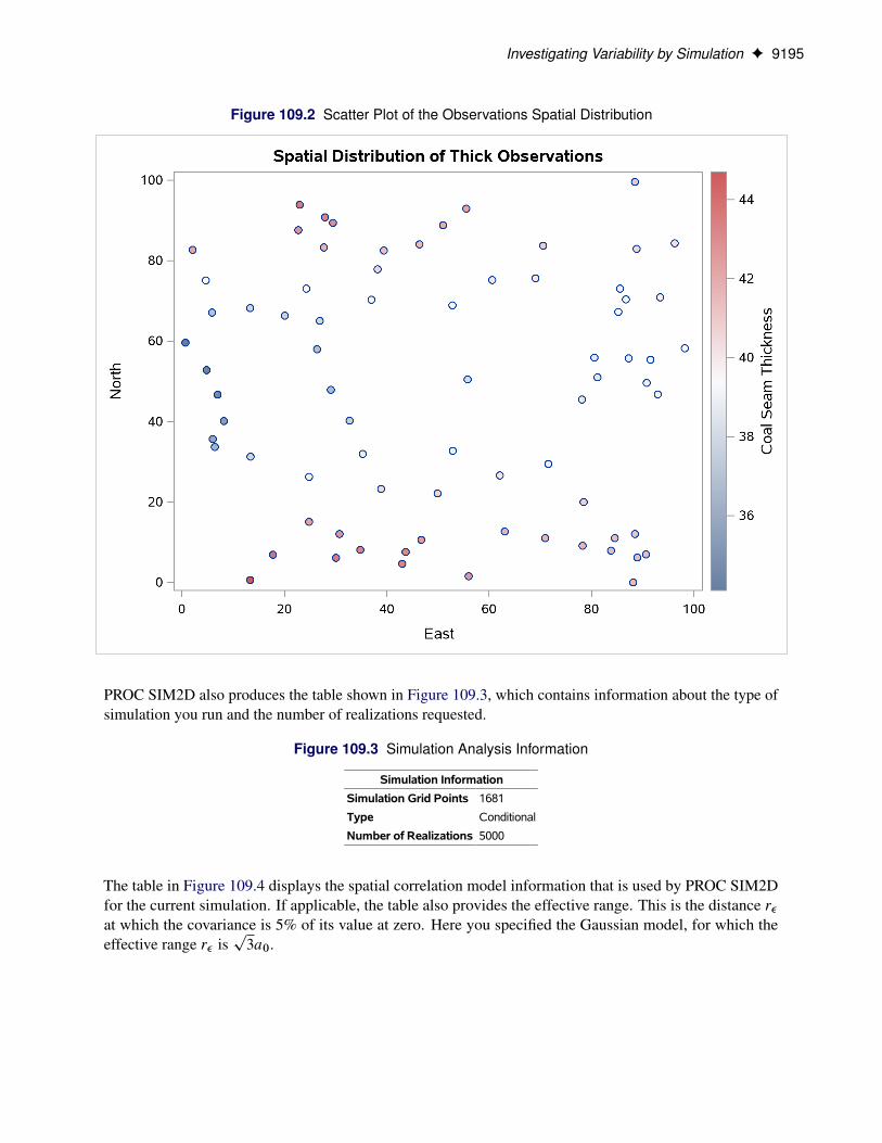
The sample locations are then plotted in Figure 109.2. The figure clearly shows some small-scale variationthat is typical of spatial data.
Investigating Variability by Simulation F 9195
Figure 109.2 Scatter Plot of the Observations Spatial Distribution
PROC SIM2D also produces the table shown in Figure 109.3, which contains information about the type ofsimulation you run and the number of realizations requested.
Figure 109.3 Simulation Analysis Information
Simulation Information
Simulation Grid Points 1681
Type Conditional
Number of Realizations 5000
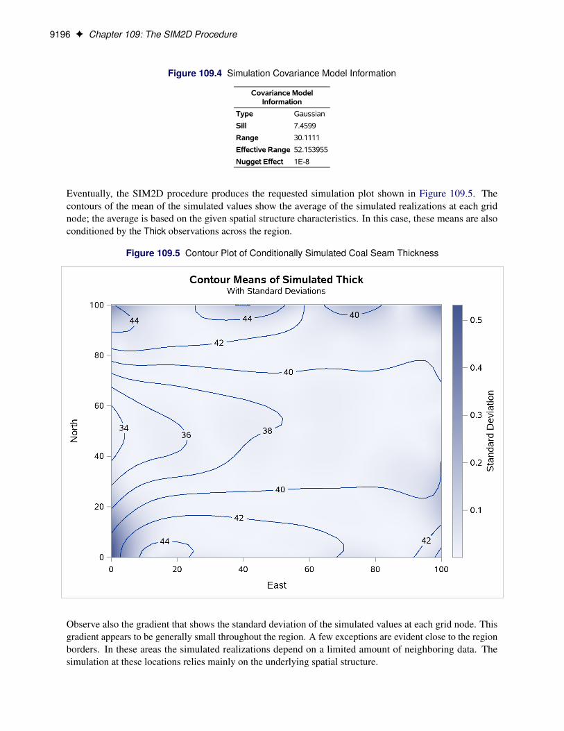
The table in Figure 109.4 displays the spatial correlation model information that is used by PROC SIM2Dfor the current simulation. If applicable, the table also provides the effective range. This is the distance r�at which the covariance is 5% of its value at zero. Here you specified the Gaussian model, for which theeffective range r� is
p3a0.
9196 F Chapter 109: The SIM2D Procedure
Figure 109.4 Simulation Covariance Model Information
Covariance ModelInformation
Type Gaussian
Sill 7.4599
Range 30.1111
Effective Range 52.153955
Nugget Effect 1E-8
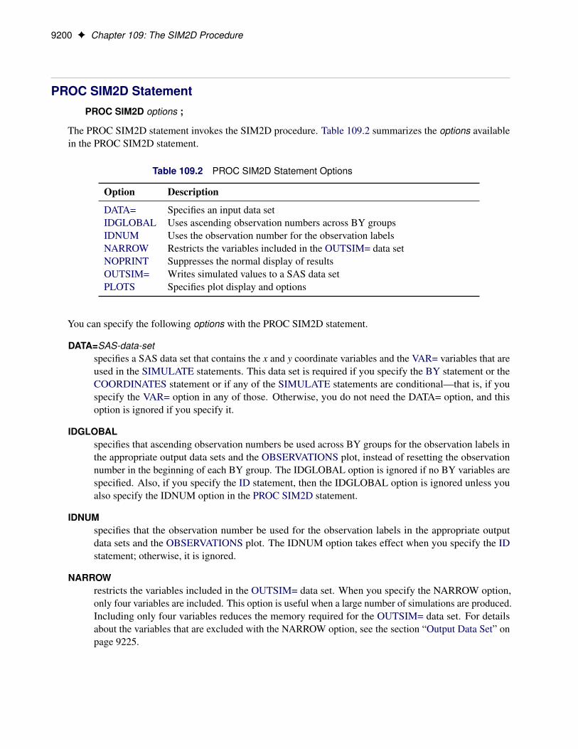
Eventually, the SIM2D procedure produces the requested simulation plot shown in Figure 109.5. Thecontours of the mean of the simulated values show the average of the simulated realizations at each gridnode; the average is based on the given spatial structure characteristics. In this case, these means are alsoconditioned by the Thick observations across the region.
Figure 109.5 Contour Plot of Conditionally Simulated Coal Seam Thickness
Observe also the gradient that shows the standard deviation of the simulated values at each grid node. Thisgradient appears to be generally small throughout the region. A few exceptions are evident close to the regionborders. In these areas the simulated realizations depend on a limited amount of neighboring data. Thesimulation at these locations relies mainly on the underlying spatial structure.

Investigating Variability by Simulation F 9197
In addition to the simulation analysis, you can use the PROC SIM2D output to obtain statistical informationabout the simulated values at selected locations. Assume that you would like some basic statistics for theextreme southwest point at (East=0, North=0) and the point (East=75, North=75) toward the northeast cornerof the region. You use the following DATA step to select the realizations for these points from the OUTSIM=output data set:
data selected;set sim(where=((gxc=0 and gyc=0) or (gxc=75 and gyc=75)));label gxc = "X-coord";label gyc = "Y-coord";
run;
Then, you use PROC SORT to sort the selected data set entries and PROC MEANS to produce the simulationstatistics for the selected points. The following statements yield the mean, standard deviation, and maximumvalues of the 5,000 realizations of the Thick values at each one of the selected locations:
proc sort data=selected;by gxc gyc;
run;proc means data=selected Mean Std Max;
class gxc gyc;ways 2;where ( ((gxc = 0) & (gyc = 0))
| ((gxc = 75) & (gyc = 75)));var SValue;
run;
ods graphics off;
The requested statistics for the grid points (East=0, North=0) and (East=75,North=75) are shown in Fig-ure 109.6.
Figure 109.6 Simulation Statistics at Grid Points (East=0, North=0) and (East=75, North=75)
Using PROC SIM2D for Spatial Simulation
The MEANS Procedure
Analysis Variable : SVALUE Simulated Value at Grid Point
X-coord Y-coord N Obs Mean Std Dev Maximum
0 0 5000 40.6968472 0.5328597 42.6616357
75 75 5000 40.1090845 0.0024556 40.1197239
“Example 109.2: Variability at Selected Locations” on page 9233 shows you how to perform a simulation at aset of selected locations rather than on a domain-wide grid, and how to obtain more detailed statistics fromthe simulation.

9198 F Chapter 109: The SIM2D Procedure
Syntax: SIM2D ProcedureThe following statements are available in the SIM2D procedure:
PROC SIM2D options ;BY variables ;COORDINATES coordinate-variables ;GRID grid-options ;ID variable ;RESTORE store-options ;SIMULATE simulate-options ;MEAN mean-options ;
The SIMULATE and MEAN statements are hierarchical; you can specify any number of SIMULATEstatements, but you must specify at least one. If you specify a MEAN statement, it refers to the precedingSIMULATE statement. If you omit the MEAN statement, a zero-mean model is simulated.
You must specify a single COORDINATES statement to identify the x and y coordinate variables in the inputdata set when you perform a conditional simulation. You must also specify a single GRID statement tospecify the grid information.
Table 109.1 outlines the options available in PROC SIM2D classified by function.
Table 109.1 Options Available in the SIM2D Procedure
Task Statement Option
Data Set OptionsSpecify an input data set PROC SIM2D DATA=Specify a grid data set GRID GDATA=Specify labels for individual grid points or in 1-D GRID LABELSpecify correlation model and parameters SIMULATE MDATA=Write simulated values PROC SIM2D OUTSIM=Specify plot display and options PROC SIM2D PLOTSSpecify a quadratic form data set MEAN QDATA=Specify plot display and options PROC SIM2D PLOTS
Declaring the Role of VariablesSpecify variables to define analysis subgroups BYSpecify a variable with observation labels IDSpecify the conditioning variable SIMULATE VAR=Specify the x and y coordinate variables in the DATA=data set
COORDINATES XC= YC=
Specify the x and y coordinate variables in the GDATA=data set
GRID XC= YC=
Specify the constant coefficient variable in the QDATA=data set
MEAN CONST=
Specify the linear x coefficient variable in the QDATA=data set
MEAN CX=

Syntax: SIM2D Procedure F 9199
Table 109.1 continued
Task Statement Option
Specify the linear y coefficient variable in the QDATA=data set
MEAN CY=
Specify the quadratic x coefficient variable in theQDATA= data set
MEAN CXX=
Specify the quadratic y coefficient variable in theQDATA= data set
MEAN CYY=
Specify the quadratic xy coefficient variable in theQDATA= data set
MEAN CXY=
Controlling the SimulationSpecify the number of grid points in one-dimensionalcases
GRID NPTS=
Specify the number of realizations SIMULATE NUMREAL=Specify the seed value for the random generator SIMULATE SEED=
Controlling the Mean Quadratic SurfaceSpecify the CONST term MEAN CONST=Specify the linear x term MEAN CX=Specify the linear y term MEAN CY=Specify the quadratic x term MEAN CXX=Specify the quadratic y term MEAN CYY=Specify the quadratic cross term MEAN CXY=
Controlling the Semivariogram ModelSpecify an angle for an anisotropic model SIMULATE ANGLE=Specify nested angles SIMULATE ANGLE=(a1; : : : ; ak)Specify a functional form SIMULATE FORM=Specify nested functional forms SIMULATE FORM=(f1; : : : ; fk)Specify a nugget effect SIMULATE NUGGET=Specify a range parameter SIMULATE RANGE=Specify nested range parameters SIMULATE RANGE=(r1; : : : ; rk)Specify a minor-major axis ratio for an anisotropic model SIMULATE RATIO=Specify nested minor-major axis ratios SIMULATE RATIO=(ra1; : : : ; rak)Specify a scale parameter SIMULATE SCALE=Specify nested scale parameters SIMULATE SCALE=(s1; : : : ; sk)Specify item store with correlation information RESTORE IN=Specify model and parameters from an item store SIMULATE STORESELECT
9200 F Chapter 109: The SIM2D Procedure
PROC SIM2D StatementPROC SIM2D options ;
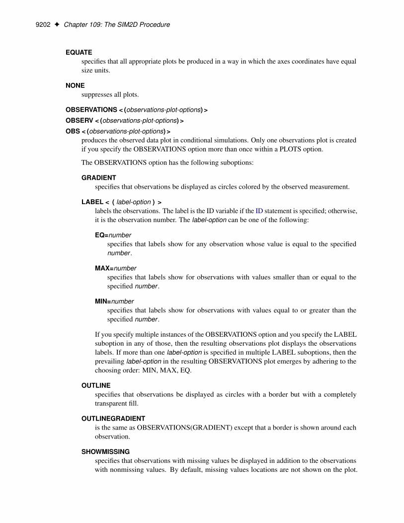
The PROC SIM2D statement invokes the SIM2D procedure. Table 109.2 summarizes the options availablein the PROC SIM2D statement.
Table 109.2 PROC SIM2D Statement Options
Option Description
DATA= Specifies an input data setIDGLOBAL Uses ascending observation numbers across BY groupsIDNUM Uses the observation number for the observation labelsNARROW Restricts the variables included in the OUTSIM= data setNOPRINT Suppresses the normal display of resultsOUTSIM= Writes simulated values to a SAS data setPLOTS Specifies plot display and options
You can specify the following options with the PROC SIM2D statement.
DATA=SAS-data-setspecifies a SAS data set that contains the x and y coordinate variables and the VAR= variables that areused in the SIMULATE statements. This data set is required if you specify the BY statement or theCOORDINATES statement or if any of the SIMULATE statements are conditional—that is, if youspecify the VAR= option in any of those. Otherwise, you do not need the DATA= option, and thisoption is ignored if you specify it.
IDGLOBALspecifies that ascending observation numbers be used across BY groups for the observation labels inthe appropriate output data sets and the OBSERVATIONS plot, instead of resetting the observationnumber in the beginning of each BY group. The IDGLOBAL option is ignored if no BY variables arespecified. Also, if you specify the ID statement, then the IDGLOBAL option is ignored unless youalso specify the IDNUM option in the PROC SIM2D statement.
IDNUMspecifies that the observation number be used for the observation labels in the appropriate outputdata sets and the OBSERVATIONS plot. The IDNUM option takes effect when you specify the IDstatement; otherwise, it is ignored.
NARROWrestricts the variables included in the OUTSIM= data set. When you specify the NARROW option,only four variables are included. This option is useful when a large number of simulations are produced.Including only four variables reduces the memory required for the OUTSIM= data set. For detailsabout the variables that are excluded with the NARROW option, see the section “Output Data Set” onpage 9225.

PROC SIM2D Statement F 9201
NOPRINTsuppresses the normal display of results. The NOPRINT option is useful when you want only to createone or more output data sets with the procedure. NOTE: This option temporarily disables the OutputDelivery System (ODS); see the section “ODS Graphics” on page 9227 for more information.
OUTSIM=SAS-data-setspecifies a SAS data set in which to store the simulation values, iteration number, simulate statementlabel, variable name, and grid location. For details, see the section “Output Data Set” on page 9225.
PLOTS < (global-plot-option) > < = plot-request< (options) > >
PLOTS < (global-plot-option) > < = (plot-request< (options) > < ... plot-request< (options) > >) >controls the plots produced through ODS Graphics. When you specify only one plot request, you canomit the parentheses around the plot request. Here are some examples:
plots=noneplots=observplots=(observ(outl) sim)plots=(sim(fill=mean line=sd obs=grad) sim(fill=sd))
ODS Graphics must be enabled before plots can be requested. For example:
ods graphics on;
proc sim2d data=thick outsim=sim;coordinates xc=East yc=North;simulate var=Thick numreal=5000 seed=79931
scale=7.4599 range=30.1111 form=gauss;mean 40.1173;grid x=0 to 100 by 2.5 y=0 to 100 by 2.5;
run;
ods graphics off;
For more information about enabling and disabling ODS Graphics, see the section “Enabling andDisabling ODS Graphics” on page 623 in Chapter 21, “Statistical Graphics Using ODS.”
By default, no graphs are created; you must specify the PLOTS= option to make graphs.
The following global-plot-option is available:
ONLYproduces only plots that are specifically requested.
The following individual plot-requests and plot options are available:
ALLproduces all appropriate plots. You can specify other options with ALL. For example, to requestall appropriate plots and an additional simulation plot, specify PLOTS=(ALL SIM).
9202 F Chapter 109: The SIM2D Procedure
EQUATEspecifies that all appropriate plots be produced in a way in which the axes coordinates have equalsize units.
NONEsuppresses all plots.
OBSERVATIONS < (observations-plot-options) >
OBSERV < (observations-plot-options) >
OBS < (observations-plot-options) >produces the observed data plot in conditional simulations. Only one observations plot is createdif you specify the OBSERVATIONS option more than once within a PLOTS option.
The OBSERVATIONS option has the following suboptions:
GRADIENTspecifies that observations be displayed as circles colored by the observed measurement.
LABEL < ( label-option ) >labels the observations. The label is the ID variable if the ID statement is specified; otherwise,it is the observation number. The label-option can be one of the following:
EQ=numberspecifies that labels show for any observation whose value is equal to the specifiednumber .
MAX=numberspecifies that labels show for observations with values smaller than or equal to thespecified number .
MIN=numberspecifies that labels show for observations with values equal to or greater than thespecified number .
If you specify multiple instances of the OBSERVATIONS option and you specify the LABELsuboption in any of those, then the resulting observations plot displays the observationslabels. If more than one label-option is specified in multiple LABEL suboptions, then theprevailing label-option in the resulting OBSERVATIONS plot emerges by adhering to thechoosing order: MIN, MAX, EQ.
OUTLINEspecifies that observations be displayed as circles with a border but with a completelytransparent fill.
OUTLINEGRADIENTis the same as OBSERVATIONS(GRADIENT) except that a border is shown around eachobservation.
SHOWMISSINGspecifies that observations with missing values be displayed in addition to the observationswith nonmissing values. By default, missing values locations are not shown on the plot.

PROC SIM2D Statement F 9203
If you specify multiple instances of the OBSERVATIONS option and you specify theSHOWMISSING suboption in any of those, then the resulting observations plot displays theobservations with missing values.
If you omit any of the GRADIENT, OUTLINE, and OUTLINEGRADIENT suboptions, theOUTLINEGRADIENT is the default suboption. If you specify multiple instances of the OBSER-VATIONS option or multiple suboptions for OBSERVATIONS, then the resulting observationsplot honors the last specified GRADIENT, OUTLINE, or OUTLINEGRADIENT suboption.
SIMULATION < (sim-plot-options) >
SIM < (sim-plot-options) >specifies that simulation plots be produced. You can specify the SIM option multiple times in thesame PLOTS option to request instances of plots with the following sim-plot-options:
ALPHA=numberspecifies a parameter to obtain the confidence level for constructing confidence limits basedon the simulation standard deviation. The value of number must be between 0 and 1, andthe confidence level is 1�number . The default is ALPHA=0.05; this corresponds to theconfidence level of 95%. The ALPHA= suboption is used only for simulation plots in onedimension, and it is incompatible with the FILL and LINE suboptions.
CLONLYspecifies that only the confidence limits be shown in a simulation plot without the simulationmean. This suboption can be useful for identifying confidence limits when the simulationstandard deviation is small at the simulation locations. CLONLY is used only for simulationband plots of simulations on a linear grid, and it is incompatible with the FILL and LINEsuboptions.
CONNPspecifies that grid points that you provide as individual simulation locations be connectedwith a line on the area map. This suboption is ignored when you have a single grid point, aprediction grid in two dimensions, or when you also specify the NOMAP suboption. TheCONNP suboption is incompatible with the FILL and LINE suboptions.
FILL=NONE | MEAN | SDproduces a surface plot for either the values of the means or the standard deviations.FILL=SD is the default. However, if you omit the FILL suboption the behavior dependson the LINE suboption as follows: If you specify LINE=NONE or entirely omit the LINEsuboption, then the FILL suboption is set to its default value. If LINE=PRED or LINE=SE,then the FILL suboption is set to the same value as the LINE suboption.
LINE=NONE | MEAN | SDproduces a contour line plot for either the values of the means or the standard deviations.LINE=MEAN is the default. However, if you omit the LINE suboption the behavior dependson the FILL suboption as follows: If you specify FILL=NONE or entirely omit the FILLsuboption, then the LINE suboption is set to its default value. If FILL=PRED or FILL=SE,then the LINE suboption is set to the same value as the FILL suboption.

9204 F Chapter 109: The SIM2D Procedure
NOMAPspecifies that the simulation plot be produced without a map of the domain where you haveobservations. The NOMAP suboption is used in the case of simulation in one dimension or atindividual points. It is ignored in the case of unconditional simulation, and it is incompatiblewith the FILL and LINE suboptions.
OBS=obs-optionsproduces an overlaid scatter plot of the observations in addition to the specified contour plots.The following obs-options are available:
GRADspecifies that observations be displayed as circles colored by the observed measurement.The same color gradient displays the means surface and the observations. The condi-tional simulation honors the observed values, so the means surface at the observationlocations has the same color as the corresponding observations.
LINEGRADis the same as OBS=GRAD except that a border is shown around each observation.This option is useful for identifying the location of observations where the standarddeviations are small, because at these points the color of the observations and the colorof the surface are indistinguishable.
NONEspecifies that no observations be displayed.
OUTLspecifies that observations be displayed as circles with a border but with a completelytransparent fill.
OBS=NONE is the default when you have a grid in two dimensions, and OBS=LINEGRADis the default used in the area map when you specify a conditional simulation in onedimension.
SHOWDspecifies that the horizontal axis in scatter plots of linear simulation grids show the distancebetween grid points instead of the grid points’ coordinates. When the area map is displayed,the simulation locations are also connected with a line. In all other grid configurations theSHOWD suboption is ignored, and it is incompatible with the FILL and LINE suboptions.
SHOWPspecifies that the grid points in band plots of linear simulation grids be shown as marks onthe band plot. In all other grid configurations the SHOWP suboption is ignored, and it isincompatible with the FILL and LINE suboptions.
TYPE=BAND | BOXrequests a particular type of plot when you have a linear grid, regardless of the default SIMplot behavior in this case. The TYPE suboption is incompatible with the FILL and LINEsuboptions.
If you specify multiple instances of the ALPHA, FILL, LINE, OBS, or TYPE suboptions in thesame SIM option, then the resulting simulation plot honors the last value specified for any of the

BY Statement F 9205
suboptions. Any combination where you specify FILL=NONE and LINE=NONE is not available.When the simulation grid is in two dimensions, only the FILL, LINE, and OBS suboptions apply.If you specify incompatible suboptions in the same SIM plot, then the plot instance is skipped.
The SIM option produces a surface or contour line plot for grids in two dimensions and a bandplot or box plot for grids in one dimension or individual points. In two dimensions the plotillustrates the means and standard deviations of the simulation realizations at each grid point. Bydefault, when you specify a linear grid with fewer than 10 points, PROC SIM2D produces a SIMbox plot that depicts the simulation distribution at each point. For 10 or more points in a lineargrid, the SIM plot is a band plot of the simulation means and the confidence limits at the 95%confidence level. You can override the default behavior in linear grids with the TYPE suboption.Simulation at individual locations always produces a SIM box plot.
In cases of conditional simulation in one dimension or at individual points an area map isproduced that shows the observations and the grid points. Band plots of linear grids display thegrid points as a line on the map. When you specify individual simulation locations, the gridpoints are indicated with marks on the area map. The area map appears on the side of conditionalsimulation band plots or box plots, unless you specify the NOMAP suboption. You can also labelindividual grid points or the ends of linear grid segments with the LABEL option of the GRIDstatement.
SEMIVARIOGRAM < (semivar-plot-option) >
SEMIVAR < (semivar-plot-option) >specifies that the semivariogram used for the simulation be produced. You can use the followingsemivar-plot-option:
MAXD=numberspecifies a positive value for the upper limit of the semivariogram horizontal axis of distance.The SEMIVARIOGRAM plot extends by default to a distance that depends on the correlationmodel range. You can use the MAXD= option to adjust the default maximum distance valuefor the plot.
The SEMIVARIOGRAM option produces a plot for each correlation model that you specify foryour simulation tasks. In an anisotropic case, the plot is not produced if you assign differentanisotropy angles for different model components. The only exception is when you specify zonalcomponents at right angles with the nonzonal model components. Also, the SEMIVARIOGRAMoption is ignored for models that consist of purely zonal components.
BY StatementBY variables ;
You can specify a BY statement in PROC SIM2D to obtain separate analyses of observations in groups thatare defined by the BY variables. When a BY statement appears, the procedure expects the input data set to besorted in order of the BY variables. If you specify more than one BY statement, only the last one specified isused.
If your input data set is not sorted in ascending order, use one of the following alternatives:
9206 F Chapter 109: The SIM2D Procedure
� Sort the data by using the SORT procedure with a similar BY statement.
� Specify the NOTSORTED or DESCENDING option in the BY statement in the SIM2D procedure.The NOTSORTED option does not mean that the data are unsorted but rather that the data are arrangedin groups (according to values of the BY variables) and that these groups are not necessarily inalphabetical or increasing numeric order.
� Create an index on the BY variables by using the DATASETS procedure (in Base SAS software).
In PROC SIM2D it makes sense to use the BY statement only in conditional simulations where observationsare involved. In particular, using the BY statement assumes that you have specified an input data set withthe DATA= option in the PROC SIM2D statement. In PROC SIM2D if you omit the VAR= option in theSIMULATE statement, then this is a request for unconditional simulation even if you have specified theDATA= option in the PROC SIM2D statement. Therefore, it is possible to specify the BY statement andrequest mixed types of simulations by specifying multiple SIMULATE statements in the same PROC SIM2Dstep.
A special case occurs when you omit the DATA= option in the PROC SIM2D statement, your unconditionalsimulation correlation model input comes from an item store in the RESTORE statement, and this store hasits own BY groups. The SIM2D procedure exhibits then a BY-like behavior, even though you specified noBY statement. This behavior enables you to distinguish the simulation tasks that depend on models in thedifferent store BY groups.
For more information about BY-group processing, see the discussion in SAS Language Reference: Concepts.For more information about the DATASETS procedure, see the discussion in the Base SAS Procedures Guide.
COORDINATES StatementCOORDINATES coordinate-variables ;
The two options in the COORDINATES statement give the name of the variables in the DATA= data set thatcontains the values of the x and y coordinates of the conditioning data. You must specify the COORDINATESstatement when you specify an input data set with the DATA= option in the PROC SIM2D statement.
Only one COORDINATES statement is allowed, and it is applied to all SIMULATE statements that have theVAR= specification. In other words, it is assumed that all the VAR= variables in all SIMULATE statementshave the same x and y coordinates.
You can abbreviate the COORDINATES statement as COORD.
XCOORD=(variable-name)
XC=(variable-name)gives the name of the variable that contains the x coordinate of the data in the DATA= data set.
YCOORD=(variable-name)
YC=(variable-name)gives the name of the variable that contains the y coordinate of the data locations in the DATA= dataset.

GRID Statement F 9207
GRID StatementGRID grid-options < / option > ;
The GRID statement specifies the grid of spatial locations at which to perform the simulations. A singleGRID statement is required and is applied to all SIMULATE statements. Specify the grid in one of thefollowing three ways:
� Specify the x and y coordinates explicitly for a grid in two dimensions.
� Specify the NPTS= option in addition to the x and y coordinates to define a grid of individual points orin one dimension.
� Specify the coordinates by using a SAS data set for a grid of individual points or in one dimension.
The GRID statement has the following grid-options:
NPTS=number | ALLcontrols specification of a grid in one dimension or a grid of individual simulation locations.
When you specify the NPTS=number option and the coordinates of two points in the GRIDDATA=data set or in both the X= and Y= options, you request a linear simulation grid. Its direction is acrossthe line defined by the specified points. The grid size is equal to the number of points that you specifyin the NPTS= option, where number � 2.
When you specify the NPTS=ALL option and the coordinates for any number of points in theGRIDDATA= data set or in each of the X= and Y= options, the SIM2D procedure performs simulationonly at the specified individual locations. Use the NPTS=ALL option to examine a set of individualpoints anywhere on the XY plane or to specify a custom grid in one dimension.
If the number of x coordinates and the number of y coordinates in the X= and Y= options, respectively,are different, then the NPTS= option is ignored; in that case, a two-dimensional grid is used accordingto the specified X= and Y= options.
If you specify a simulation grid with any number of points other than two in the GRIDDATA= data set,then the option NPTS=ALL has the same effect as omitting the NPTS= option.
X=numberX=x1; : : : ; xmX=x1 TO xm
X=x1 TO xm BY ıxspecifies the x coordinate of the grid locations.
Y=numberY=y1; : : : ; ymY=y1 TO ym
Y=y1 TO ym BY ıyspecifies the y coordinate of the grid locations.
Use the X= and Y= options of the GRID statement to specify a grid in one or two dimensions, or agrid of individual simulation locations.
For example, the following two GRID statements are equivalent:

9208 F Chapter 109: The SIM2D Procedure
GRID X=1,2,3,4,5 Y=0,2,4,6,8,10;
GRID X=1 TO 5 Y=0 to 10 by 2;
In the following example, the first GRID statement produces a grid in two dimensions. The secondstatement produces simulation output only for the four individual points at the locations (1,0), (2,5),(3,7), and (4,10) on the XY plane.
GRID X=1 TO 4 Y=0,5,7,10;
GRID X=1 TO 4 Y=0,5,7,10 NPTS=ALL;
In the next example, the first GRID statement specifies a 2-by-2 grid in two dimensions. The secondGRID statement specifies a linear grid of eight points. The grid is in the direction of the line defined bythe specified points (2,8) and (3,5) on the XY plane and it extends between these two points.
GRID X=2,3 Y=8,5;
GRID x=2,3 Y=8,5 NPTS=8;
The last example shows a GRID statement that specifies a linear grid made of seven points across theY axis. In this case, the syntax is sufficient to fully define a linear grid without the NPTS= option.
GRID X=5 Y=3 TO 9;
To specify grid locations from a SAS data set, you must provide the name of the data set and thevariables that contain the values of the x and y coordinates.
GRIDDATA=SAS-data-set
GDATA=SAS-data-setspecifies a SAS data set that contains the x and y grid coordinates. Use the GRIDDATA= option of theGRID statement to specify a grid in one dimension or a grid of individual simulation locations.
XCOORD=(variable-name)
XC=(variable-name)gives the name of the variable that contains the x coordinate of the grid locations in the GRIDDATA=data set.
YCOORD=(variable-name)
YC=(variable-name)gives the name of the variable that contains the y coordinate of the grid locations in the GRIDDATA=data set.
You can specify the following option in the GRID statement after a slash (/):

ID Statement F 9209
LABEL < (suboption) > = (character-list)specifies labels to tag grid points in simulation plots when you use grids in one dimension. You canspecify one or more such labels as quoted strings in the character-list .
When the number of labels in the character-list exceeds the number of points in your grid, the labels inthe list are used sequentially and any labels in excess are ignored. When the number of labels in thecharacter-list is smaller than the number of points in your grid, the behavior is as follows:
� If an area map is included in the simulation plot, then blank labels are assigned to the remainingnonlabeled grid points on the map.
� For the simulation band and box plots, the coordinates of nonlabeled grid points are automaticallyassigned as their labels.
If the grid points are collinear and the horizontal axis displays distance, then two labels appear bydefault in the simulation plot. These are assigned to the first and the last points of the grid to helpidentify the ends of the linear grid segment on the plot map. This label pair is shown only when theplot includes an area map. Specifically, the two labels appear when you request simulation band plots,or simulation box plots for which you specify the SIM(SHOWD) suboption, if applicable. The twolabels do not appear if you specify explicitly the NOMAP suboption in the PLOTS=SIM option.
The two labels have default values, unless you choose to specify your own labels with the LABEL=option. If you specify more than two labels in the character-list under these conditions, then only thefirst and last labels in the list are used; any additional labels in between are ignored.
The LABEL= option has the following suboption:
ALLspecifies that all individual points in the grid are assigned sequentially the labels you specify inthe LABEL(ALL)= option when the SIM(SHOWD) suboption is applicable and specified in asimulation box plot. In all other cases, the ALL suboption is ignored.
The ALL suboption enables you to override the default behavior when the SIM(SHOWD)suboption is specified (the default behavior is to display labels only for the first and last gridpoints). As a result, you can use the ALL suboption to label grid points in both conditional andunconditional simulation tasks regardless of whether you specify the NOMAP suboption in thePLOTS=SIM option.
The LABEL= option is ignored when you produce simulation plots of grids in two dimensions.
ID StatementID variable ;
The ID statement specifies which variable to include for identification of the observations in the labels andtool tips of the OBSERVATIONS plot and the tool tips of the SIM plot. The ID statement has an effect onlywhen you perform conditional simulation.
In the SIM2D procedure you can specify only one ID variable in the ID statement. If no ID statement isgiven, then PROC SIM2D uses the observation number in the plots.

9210 F Chapter 109: The SIM2D Procedure
RESTORE StatementRESTORE IN=store-name < / option > ;
The RESTORE statement specifies an item store that provides spatial correlation model input for the PROCSIM2D simulation tasks. An item store is a binary file defined by the SAS System. You cannot modify thecontents of an item store. The SIM2D procedure can use only item stores created by PROC VARIOGRAM.
Item stores enable you to use saved correlation models without having to repeat specification of these modelsin the SIMULATE statement. In principle, an item store contains the chosen model from a model fittingprocess in PROC VARIOGRAM. If more than one model form is fitted, then all successful fits are includedin the item store. In this case, you can choose any of the available models to use for simulation with theSTORESELECT(MODEL=) option in the SIMULATE statement. Successfully fitted models might includequestionable fits, which are so flagged when you specify the INFO option to display model names.
The store-name is a usual one- or two-level SAS name, as for SAS data sets. If you specify a one-levelname, then the item store resides in the WORK library and is deleted at the end of the SAS session. Sinceitem stores are often used for postprocessing tasks, typical usage specifies a two-level name of the formlibname.membername.
When you specify the RESTORE statement, the default output contains some general information about theinput item store. This information includes the store name, label (if assigned), the data set that was used tocreate the store, BY group information, the procedure that created the store, and the creation date.
You can specify the following option in the RESTORE statement after a slash (/):
INFO < ( info-options ) >specifies that additional information about the input item store be printed. This information is providedin two ODS tables. One table displays the variables in the item store, in addition to the mean andstandard deviation for each of them. These statistics are based on the observations that were used toproduce the store results. The second table shows the model on top of the list of all fitted models foreach direction angle in the item store. The INFO option has the following info-options:
DETAILS
DETspecifies that more detailed information be displayed about the input item store. This optionproduces the full list of models for each direction angle in the item store, in addition to the modelequivalence class. For more information about classes of equivalence, see the section “Classes ofEquivalence” on page 10698 in Chapter 128, “The VARIOGRAM Procedure.” The DETAILSoption is ignored if the input item store contains information about a single fitted model.
ONLYspecifies that only information about the input item store without any simulation tasks bedisplayed.
Each variable in an item store has a mean value that is passed to PROC SIM2D and used in simulations.If the mean in the item store is a missing value, then a zero mean is used by default. Specify the “MEANStatement” on page 9220 to override the mean information in the item store. For example, if you want to useonly the correlation model in the item store and exclude the accompanying mean, then explicitly specify azero mean in the “MEAN Statement” on page 9220.
SIMULATE Statement F 9211
When you specify an input item store with the RESTORE statement in PROC SIM2D, all the DATA= inputdata set variables must match input item store variables. If there are BY groups in the input DATA= set or inthe input RESTORE variables, then PROC SIM2D handles the different cases as follows:
� If both PROC SIM2D has BY groups and the RESTORE statement has BY groups, then the analysisvariables must match. This matching assumes implicitly that in each BY group of PROC SIM2Dand the item store, the corresponding set of observations and correlation model comes from the samerandom field. This assumption is valid if you use the same data set, first in PROC VARIOGRAM to fita model and save it in the item store, and then in PROC SIM2D to run simulations with the resultingcorrelation models.
� If PROC SIM2D has BY groups but the item store does not, then the item store is accepted only ifthe procedure and the item store analysis variables match. In this case, the same item store modelchoice iterates across the BY groups of the input data. You are advised to proceed with caution: eachBY group in the input DATA= set corresponds to a different realization of a random field. Hence, byusing the same correlation model for simulation purposes, you implicitly assume that all these differentrealizations are instances of the same random field.
� If PROC SIM2D has an input DATA= set and no BY groups but the item store has BY groups, then theitem store is rejected
� If PROC SIM2D has no input DATA= set and the item store has BY groups, then PROC SIM2D runsunconditional simulations for the models in the store BY groups. See also the BY statement for moreabout the behavior in this case.
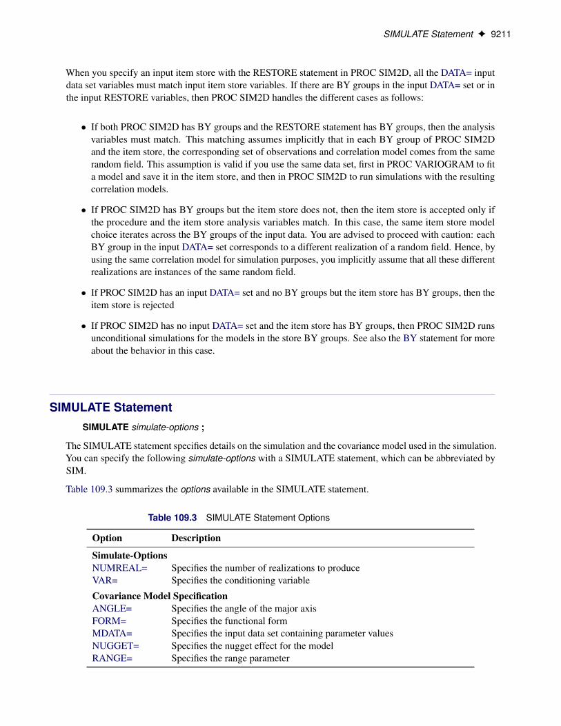
SIMULATE StatementSIMULATE simulate-options ;
The SIMULATE statement specifies details on the simulation and the covariance model used in the simulation.You can specify the following simulate-options with a SIMULATE statement, which can be abbreviated bySIM.
Table 109.3 summarizes the options available in the SIMULATE statement.
Table 109.3 SIMULATE Statement Options
Option Description
Simulate-OptionsNUMREAL= Specifies the number of realizations to produceVAR= Specifies the conditioning variable
Covariance Model SpecificationANGLE= Specifies the angle of the major axisFORM= Specifies the functional formMDATA= Specifies the input data set containing parameter valuesNUGGET= Specifies the nugget effect for the modelRANGE= Specifies the range parameter

9212 F Chapter 109: The SIM2D Procedure
Table 109.3 continued
Option Description
RATIO= Specifies the ratio of the minor axis to the major axisSCALE= Specifies the scale (or sill) parameterSEED= Specifies the seed to use for the random number generatorSINGULAR= Gives the singularity criterionSMOOTH= Specifies the smoothness parameterSTORESELECT Uses information from an input item store for prediction
NUMREAL=number
NUMR=number
NR=numberspecifies the number of realizations to produce for the spatial process specified by the covariance model.As a result, the number of observations in the OUTSIM= data set contributed by a given SIMULATEstatement is the product of the NUMREAL= value and the number of grid points. This can cause theOUTSIM= data set to become large even for moderate values of the NUMREAL= option.
VAR=(variable-name)specifies the single numeric variable used as the conditioning variable in the simulation. In other words,the simulation is conditional on the values of the VAR= variable found in the DATA= data set. Ifyou omit the VAR= option or if all observations of the VAR= variable are missing values, then thesimulation is unconditional. Since multiple SIMULATE statements are allowed, you can perform bothunconditional and conditional simulations with a single PROC SIM2D statement.
Covariance Model Specification
You can specify a semivariogram or covariance model in three ways:
� You specify the required parameters SCALE, RANGE, FORM, and SMOOTH (if you specify theMATERN form), and possibly the optional parameters NUGGET, ANGLE, and RATIO, explicitly inthe SIMULATE statement.
� You specify an MDATA= data set. This data set contains variables that correspond to the requiredparameters SCALE, RANGE, FORM, and SMOOTH (if you specify the MATERN form), and,optionally, variables for the NUGGET, ANGLE, and RATIO parameters.
� You can specify an input item store in the RESTORE statement. The item store contains one ormore correlation models for one or more direction angles. You can specify these models in theSTORESELECT option of the SIMULATE statement to run a simulation.
The three methods are mutually exclusive: you specify all parameters explicitly, they are all are read fromthe MDATA= data set, or you select a model and its parameters from an input item store. The followingsimulate-options are related to model specification:

SIMULATE Statement F 9213
ANGLE=angle | (angle1, . . . , anglek )specifies the angle of the major axis for anisotropic models, measured in degrees clockwise from theN–S axis. The default is ANGLE=0.
In the case of a nested semivariogram model with k nestings, you have the following two ways tospecify the anisotropy major axis: you can specify only one angle which is then applied to all nestedforms, or you can specify one angle for each of the k nestings.
NOTE: The syntax makes it possible to specify different angles for different forms of the nested model,but this practice is rarely used.
FORM=form | (form1, . . . , formk )specifies the functional form (type) of the semivariogram model. Use the syntax with the single form tospecify a non-nested model. Use the syntax with forms formi , i D 1; : : : ; k, to specify a nested modelwith k structures. Each of the forms can be any of the following:
CUBIC | EXPONENTIAL | GAUSSIAN | MATERN |
PENTASPHERICAL | SINEHOLEEFFECT | SPHERICAL
CUB | EXP | GAU | MAT | PEN | SHE | SPHspecify the functional form (type).
For example, the syntax
FORM=GAU
specifies a model with a single Gaussian structure. Also, the syntax
FORM=(EXP,SHE,MAT)
specifies a nested model with an exponential, a sine hole effect, and a Matérn structure. Finally
FORM=(EXP,EXP)
specifies a nested model with two structures both of which are exponential.
NOTE: In the documentation, models are named either by using their full names or by using the firstthree letters of their structures. Also, the names of different structures in a nested model are separatedby a hyphen (-). According to this convention, the previous examples illustrate how to specify a GAU,an EXP-SHE-MAT, and an EXP-EXP model, respectively, with the FORM= option.
All the supported model forms have two parameters specified by the SCALE= and RANGE= options,except for the MATERN model which has a third parameter specified by the SMOOTH= option. AFORM= value is required, unless you specify the MDATA= option or the STORESELECT option.
Computation of the MATERN covariance is numerically demanding. As a result, simulations that useMatérn covariance structures can be time-consuming.

9214 F Chapter 109: The SIM2D Procedure
MDATA=SAS-data-setspecifies the input data set that contains parameter values for the covariance or semivariogram model.The MDATA= option cannot be combined with any of the FORM= or STORESELECT options.
The MDATA= data set must contain variables named SCALE, RANGE, and FORM, and it can optionallycontain variables NUGGET, ANGLE, and RATIO. If you specify the MATERN form, then you mustalso include a variable named SMOOTH in the MDATA= data set.
The FORM variable must be a character variable, and it can assume only the values allowed in theexplicit FORM= syntax described previously. The RANGE, SCALE and SMOOTH variables must benumeric. The optional variables ANGLE, RATIO, and NUGGET must also be numeric if present.
The number of observations present in the MDATA= data set corresponds to the level of nesting of thecovariance or semivariogram model. For example, to specify a non-nested model that uses a sphericalcovariance, an MDATA= data set might contain the following statements:
data md1;input scale range form $;datalines;25 10 SPH
;
The PROC SIM2D statement to use the MDATA= specification is of the form shown in the following:
proc sim2d data=...;sim var=.... mdata=md1;
run;
This is equivalent to the following explicit specification of the covariance model parameters:
proc sim2d data=...;sim var=.... scale=25 range=10 form=sph;
run;
The following MDATA= data set is an example of an anisotropic nested model:
data md2;input scale range form $ nugget angle ratio smooth;datalines;20 8 SPH 5 35 .7 .12 3 MAT 5 0 .8 2.84 1 GAU 5 45 .5 .
;
proc sim2d data=...;sim var=.... mdata=md2;
run;
This is equivalent to the following explicit specification of the covariance model parameters:

SIMULATE Statement F 9215
proc sim2d data=...;sim var=.... scale=(20,12,4) range=(8,3,1) form=(SPH,MAT,GAU)
angle=(35,0,45) ratio=(.7,.8,.5) nugget=5 smooth=2.8;run;
This example is somewhat artificial in that it is usually hard to detect different anisotropy directions andratios for different nestings by using an experimental semivariogram. NOTE: The NUGGET variablevalue is the same for all nestings. This is always the case; the nugget effect is a single additive term forall models. For further details, see the section “The Nugget Effect” on page 5402 in Chapter 71, “TheKRIGE2D Procedure.”
The example also shows that if you specify a MATERN form in the nested model, then the SMOOTHvariable must be specified for all nestings in the MDATA= data set. You simply specify the SMOOTHvalue as missing for nestings other than MATERN.
The SIMULATE statement can be given a label. This is useful for identification in the OUTSIM= dataset when multiple SIMULATE statements are specified. For example:
proc sim2d data=...;gauss1: sim var=.... form=gau;mean ....;gauss2: sim var=.... form gau;mean ....;exp1: sim var=.... form=exp;mean ....;exp2: sim var=.... form=exp;mean ....;
run;
In the OUTSIM= data set, the values “GAUSS1,” “GAUSS2,” “EXP1,” and “EXP2” for the LABELvariable help to identify the realizations that correspond to the four SIMULATE statements. If youdo not provide a label for a SIMULATE statement, a default label of SIMn is given, where n is thenumber of unlabeled SIMULATE statements seen so far.
NUGGET=numberspecifies the nugget effect for the model. This effect is due to a discontinuity in the semivariogram asdetermined by plotting the sample semivariogram (see the section “The Nugget Effect” on page 5402in Chapter 71, “The KRIGE2D Procedure,” for details). For models without any nugget effect, theNUGGET= option is left out. The default is NUGGET=0.
RANGE=range | (range1, . . . , rangek )specifies the range parameter in the semivariogram models. In the case of a nested semivariogrammodel with k nestings, you must specify a range for each nesting.
The range parameter is the divisor in the exponent in all supported models. It has the units of distanceor distance squared for these models, and it is related to the correlation scale for the underlying spatialprocess.
See the section “Theoretical Semivariogram Models” on page 5395 in Chapter 71, “The KRIGE2DProcedure,” for details about how the RANGE= values are determined.

9216 F Chapter 109: The SIM2D Procedure
RATIO=ratio | (ratio1, . . . , ratiok )specifies the ratio of the length of the minor axis to the length of the major axis for anisotropic models.The value of the RATIO= option must be between 0 and 1. In the case of a nested semivariogrammodel with k nestings, you can specify a ratio for each nesting. The default is RATIO=1.
SCALE=scale | (scale1, . . . , scalek )specifies the scale (or sill) parameter in semivariogram models. In the case of a nested semivari-ogram model with k nestings, you must specify a scale for each nesting. The scale parameter is themultiplicative factor in all supported models; it has the same units as the variance of the VAR= variable.
See the section “Theoretical Semivariogram Models” on page 5395 in Chapter 71, “The KRIGE2DProcedure,” for details about how the SCALE= values are determined.
SEED=seed-valuespecifies the seed to use for the random number generator. The SEED= option seed-value has to be aninteger.
SINGULAR=numbergives the singularity criterion for solving the set of linear equations involved in the computation of themean and covariance of the conditional distribution associated with a given SIMULATE statement.The larger the value of the SINGULAR= option, the easier it is for the covariance matrix system to bedeclared singular. The default is SINGULAR=1E–8.
For more details about the use of the SINGULAR= option, see the section “Computational andTheoretical Details of Spatial Simulation” on page 9222.
SMOOTH=smooth | (smooth1, . . . , smoothm)specifies the smoothness parameter � > 0 in the Matérn type of semivariance structures. The specialcase � D 0:5 is equivalent to the exponential model, whereas � !1 gives the Gaussian model.
When you specify m different MATERN forms in the FORM= option, you must also provide msmoothness values in the SMOOTH option. If you must specify more than one smoothness value, thevalues are assigned sequentially to the MATERN nestings in the order the nestings are specified. Ifyou specify more smoothness values than necessary, then values in excess are ignored.
STORESELECT(ssel-options)
SSEL(ssel-options)specifies that information from an input item store be used for the prediction. You cannot combine theSTORESELECT option with any of the FORM= or MDATA= options. The STORESELECT optionhas the following ssel-options:
TYPE=field-typespecifies whether to perform isotropic or anisotropic simulation. You can choose the field-typefrom one of the following:
ISOspecifies isotropic field for the simulation.
ANIGEO | GEOspecifies a field with geometric anisotropy for the simulation.

SIMULATE Statement F 9217
ANIZON(zonal-form1, . . . , zonal-formn)ZON(zonal-form1, . . . , zonal-formn)
specifies a field with zonal anisotropy for the simulation. Each zonal-formi , i D 1; : : : ; n,can be any of the following:
CUB | EXP | GAU | MAT | PEN | SHE | SPHspecify a form for the simulation.
Each zonal-formi , i D 1; : : : ; n, is a structure in the purely zonal component of the correlationmodel in the direction angle of the minor anisotropy axis. For this reason, when you specifythe TYPE=ANIZON suboption you must also specify the nonzonal component of thecorrelation model in the MODEL= suboption of the STORESELECT option. Assume thenonzonal component has k structures; these are common across all directions and each onehas the same scale in all directions. In that sense, you use the TYPE=ANIZON suboptionto specify only the n zonal anisotropy structures of an input store (k C n)-structure nestedmodel in the direction angle of the minor anisotropy axis.
Given this specification, kCnmust be up to the maximum number of nested model structuresthat is supported by the item store. See also the MODEL= suboption of the STORESELECToption.
In conclusion, you can use an input item store for prediction with zonal anisotropy if youknow that every structure in the nonzonal model component has the same scale across alldirections. When this condition does not apply for the item store models, specify the modelparameters explicitly in the SIMULATE statement.
Computation of the MATERN covariance is numerically demanding. As a result, predictions thatuse Matérn covariance structures can be time-consuming.
If you omit the TYPE= option, the default behavior is TYPE=ISO when the input item storecontains information for only one angle or for the omnidirectional case. If you specify an itemstore with information for more than one direction, then the default behavior is TYPE=ANIGEO.
When you specify TYPE=ISO to request isotropic analysis in the presence of an item storewith information for multiple directions, you must specify the ANGLEID= suboption of theSTORESELECT option with one argument. This argument specifies which of the directionangles information to use for the isotropic analysis.
When you indicate the presence of anisotropy with the TYPE=ANIGEO or TYPE=ANIZONsuboptions of the STORESELECT option, the following conditions apply:
� You must specify the ANGLEID= suboption of the STORESELECT option to designate themajor and minor anisotropy axes. See the ANGLEID= suboption of the STORESELECToption for details.� – For TYPE=ANIGEO, ensure that you have the same scale in all anisotropy directions.
– For TYPE=ANIZON, ensure that the nonzonal component scale is the same in allanisotropy directions.
If you import a nested model, these rules also apply to each one of the nested structures.� Model ranges in the major anisotropy axis must be longer than ranges in the minor anisotropy
axis.� Any Matérn covariance structure must maintain its smoothness parameter value in all
anisotropy directions.

9218 F Chapter 109: The SIM2D Procedure
ANGLEID=angleid1 | (angleid1, angleid2)specifies which direction angles in the input item store be used for simulation. The angles areidentified by the corresponding number in the AngleID column of the “Store Models Information”table, or by the AngleID parameter in the table title when you specify the INFO(DETAILS) optionin the RESTORE statement.
If you request isotropic prediction in the TYPE= suboption of the STORESELECT option and theitem store has omnidirectional contents or information about only one angle, then the ANGLEID=option is ignored. The simulation input comes from the omnidirectional information. In the caseof a single angle, you still perform isotropic simulation and the model parameters are providedby the model in the single direction angle in the item store. However, if the item store containsinformation for more than one angle, then you must specify one angle ID in angleid1. The modelinformation from the corresponding angle is then used in your isotropic simulation.
When you specify an anisotropic simulation in the TYPE= option of the STORESELECT option,you need to have information about two perpendicular direction angles. One of them is the majorand the other is the minor anisotropy axis. You must always specify the major anisotropy axisangle ID in angleid1 and the minor anisotropy axis angle ID in angleid2. This means that therange parameters of the model forms in the angle designated by the angleid1 need to be largerthan the corresponding ranges of the forms in the angle designated by the angleid2. Conveniently,if the item store has only two angles, then you only need to specify the ID angleid1 of the majoranisotropy axis angle. If the item store has only one angle, then you cannot perform anisotropicsimulation with input from the item store.
NOTE: You can perform geometric anisotropic analysis even if the item store does not containinformation about a direction that is perpendicular to the one specified by angleid1. This ispossible due to the geometry of the ellipse. In particular, when you specify the major axis withangleid1 and an angle ID for a second direction with a corresponding smaller range, then PROCSIM2D automatically computes the minor anisotropy axis range and the necessary range ratioparameter.
Anisotropic analysis is not possible when you specify instances of the same angle in the inputitem store. It is possible that PROC VARIOGRAM produces an item store where two or moredirections can be the same if their corresponding correlation models were obtained for differentangle tolerances or bandwidths in the VARIOGRAM procedure. Consequently, you cannotspecify anisotropic simulation if the input store contains only two angles that are the same or ifyou specify angleid1 and angleid2 that correspond to equal angles.
MODEL=form | (form1, . . . , formk )specifies the theoretical semivariogram model selection to use for the simulation. Use anycombination of one, two, or three forms to describe a model in the input item store because up tothree nested structures are supported. Each formi , i D 1; : : : ; k, can be any of the following:
CUB | EXP | GAU | MAT | PEN | SHE | SPHspecify the selection model.
Computation of the MATERN covariance is numerically demanding. As a result, simulationsthat use Matérn covariance structures can be time-consuming.
All fitted models that are stored in the input item store contain information about their compo-nent parameters and also about the nugget effect if any. The SIM2D procedure retrieves this

SIMULATE Statement F 9219
information when you make a model selection in the MODEL= option, and you do not need toindividually specify a nugget effect or any other parameter of the model.
By default, the model that is ranked first among the models for a given angle in the item store isused for the simulation task. If more than one model is available in the item store, then you canspecify the MODEL= option to use a different model for the simulation.
In an anisotropic simulation, the default selection is the model that is ranked first in the directionangle of the major anisotropy axis. If you specify the TYPE=ANIGEO option, then a model thatconsists of identical structures needs to be present in the selected minor anisotropy axis angle inthe item store. If you specify the TYPE=ANIZON option, then a model with the exact same firstk structures must be present in the selected minor anisotropy axis angle, and it must feature atleast one more structure as a zonal component. The zonal component is specified separately inthe TYPE=ANIZON suboption of the STORESELECT option. Consequently, remember thatin zonal anisotropy the MODEL= suboption designates only the nonzonal component of thecorrelation model in the minor anisotropy axis direction. In all, if there are k common structuresand n structures in the purely zonal component, then k C n must be up to the maximum numberof nested model structures that is supported by the item store.
SVAR=store-var | (store-varlist)specifies one store-var item store variable or a list store-varlist of variables that are present in theitem store. This option selects one or more item store variables whose correlation models youwant to use in the current simulation task.
If you are performing a conditional simulation, then PROC SIM2D searches the input item storefor the variable that is specified in the VAR= option of the SIMULATE statement. Then, theprocedure selects the appropriate correlation model for the task. In this case, if you specify theSVAR= option, it is ignored. However, when you request an unconditional simulation and specifyinput from an item store, then you must also use SVAR= to specify a source for your correlationmodel.
In comparison to the other two ways of specifying a correlation model in PROC SIM2D, the STORES-ELECT option is quite different because you can avoid explicit specification of all parameter values ofa model. When you specify the STORESELECT option, then the corresponding scale, range, nuggeteffect, and smoothness (if appropriate) parameter values are invoked as saved attributes of the modelthat you select from the item store.
In the case of anisotropy, you specify the angles indirectly with the ANGLEID= option of theSTORESELECT option, and the ratios are computed implicitly by using the selected model ranges.Explore how to specify valid anisotropical models imported from an input item store with the twoexamples that follow.
In the first example, assume the input item store InStoreGeo contains exponential models in theangles �1 D 0ı, �2 D 45ı, and �3 D 90ı. You know in advance that all models have the same scalec1 D c2 D c3 across these directions and that the respective ranges are a1 D 15, a2 D 20, anda3 D 25 in distance units. Hence, you have a case of geometric anisotropy where the major anisotropyaxis is in the direction of angle �3 and the minor anisotropy axis is in the direction of angle �1. Thefollowing statements in PROC SIM2D use the information in the item store InStoreGeo to performsimulation under the assumption of geometric anisotropy:
9220 F Chapter 109: The SIM2D Procedure
proc sim2d data=...;restore in=InStoreGeo;simulate storeselect(model=exp type=anigeo angleid=(3,1));
run;
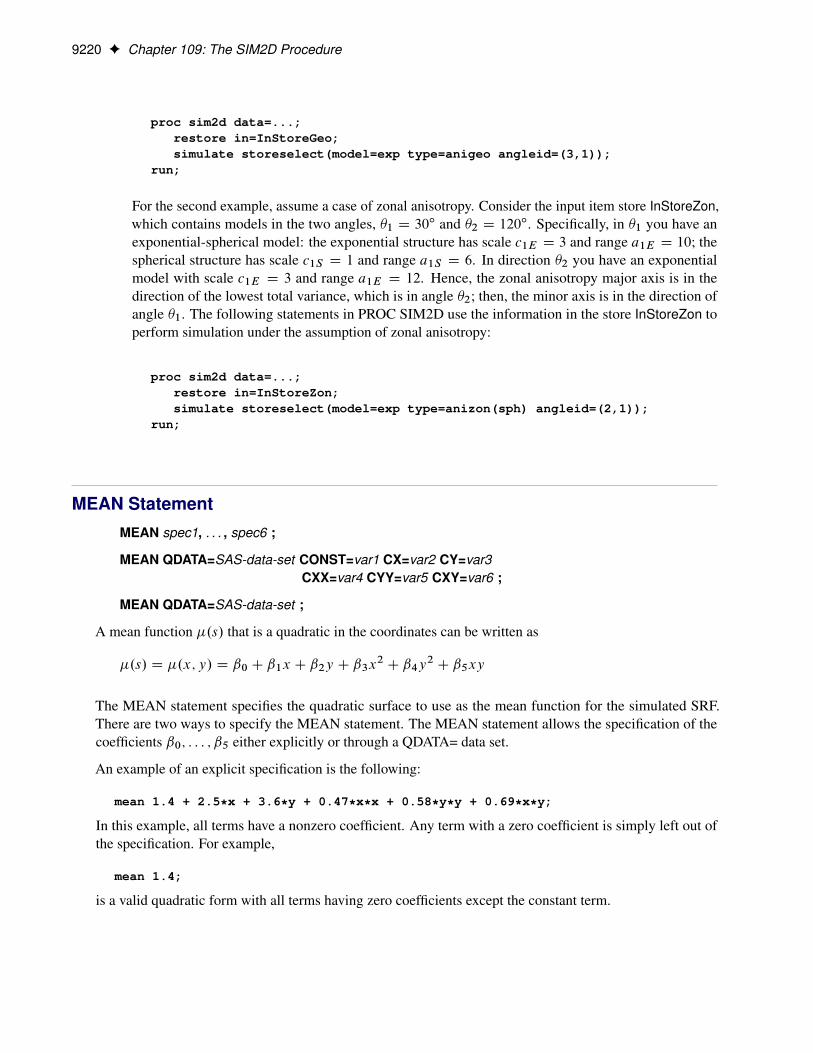
For the second example, assume a case of zonal anisotropy. Consider the input item store InStoreZon,which contains models in the two angles, �1 D 30ı and �2 D 120ı. Specifically, in �1 you have anexponential-spherical model: the exponential structure has scale c1E D 3 and range a1E D 10; thespherical structure has scale c1S D 1 and range a1S D 6. In direction �2 you have an exponentialmodel with scale c1E D 3 and range a1E D 12. Hence, the zonal anisotropy major axis is in thedirection of the lowest total variance, which is in angle �2; then, the minor axis is in the direction ofangle �1. The following statements in PROC SIM2D use the information in the store InStoreZon toperform simulation under the assumption of zonal anisotropy:
proc sim2d data=...;restore in=InStoreZon;simulate storeselect(model=exp type=anizon(sph) angleid=(2,1));
run;
MEAN StatementMEAN spec1, . . . , spec6 ;
MEAN QDATA=SAS-data-set CONST=var1 CX=var2 CY=var3CXX=var4 CYY=var5 CXY=var6 ;
MEAN QDATA=SAS-data-set ;
A mean function �.s/ that is a quadratic in the coordinates can be written as
�.s/ D �.x; y/ D ˇ0 C ˇ1x C ˇ2y C ˇ3x2C ˇ4y
2C ˇ5xy
The MEAN statement specifies the quadratic surface to use as the mean function for the simulated SRF.There are two ways to specify the MEAN statement. The MEAN statement allows the specification of thecoefficients ˇ0; : : : ; ˇ5 either explicitly or through a QDATA= data set.
An example of an explicit specification is the following:
mean 1.4 + 2.5*x + 3.6*y + 0.47*x*x + 0.58*y*y + 0.69*x*y;
In this example, all terms have a nonzero coefficient. Any term with a zero coefficient is simply left out ofthe specification. For example,
mean 1.4;
is a valid quadratic form with all terms having zero coefficients except the constant term.

MEAN Statement F 9221
An equivalent way of specifying the mean function is through the QDATA= data set. For example, the MEANstatement
mean 1.4 + 2.5*x + 3.6*y + 0.47*x*x + 0.58*y*y + 0.69*x*y;
can be alternatively specified by the following DATA step and MEAN statement:
data q1;input c1 c2 c3 c4 c5 c6;datalines;1.4 2.5 3.6 0.47 0.58 0.69
;
proc sim2d data=....;simulate ...;mean qdata=q1 const=c1 cx=c2 cy=c3 cxx=c4 cyy=c5 cxy=c6;
run;
The QDATA= data set specifies the data set containing the coefficients. The parameters CONST=, CX=, CY=,CXX=, CYY=, and CYX= specify the variables in the QDATA= data set that correspond to the constant,linear y, linear y, and so on. For any coefficient not specified in this list, the QDATA= data set is checked forthe presence of variables with default names of CONST, CX, CY, CXX, CYY, and CXY. If these variablesare present, their values are taken as the corresponding coefficients. Hence, you can rewrite the previousexample as follows:
data q1;input const cx cy cxx cyy cxy;datalines;1.4 2.5 3.6 0.47 0.58 0.69
;
proc sim2d data=....;simulate ...;mean qdata=q1;
run;
If a given coefficient does not appear in the list or in the data set with the default name, a value of zero isassumed.
If you run a simulation task with input from a RESTORE statement, then by default the simulation uses themean of the item store variable in the simulation. You can override this default behavior if you explicitlyspecify the MEAN statement with a different mean function.

9222 F Chapter 109: The SIM2D Procedure
Details: SIM2D Procedure
Computational and Theoretical Details of Spatial Simulation
Introduction
There are a number of approaches to simulating spatial random fields or, more generally, simulating sets ofdependent random variables. These include sequential indicator methods, turning bands, and the Karhunen-Loeve expansion. See Christakos (1992, Chapter 8) and Deutsch and Journel (1992, Chapter V) for details.
A particularly simple method available for Gaussian spatial random fields is the LU decomposition method.This method is computationally efficient. For a given covariance matrix, the LU D LL0 decompositionis computed once, and the simulation proceeds by repeatedly generating a vector of independent N.0; 1/random variables and multiplying by the L matrix.
One problem with this technique is memory requirements; memory is required to hold the full data and gridcovariance matrix in core. While this is especially limiting in the three-dimensional case, you can use PROCSIM2D, which handles only two-dimensional data, for moderately sized simulation problems.
Theoretical Development
It is a simple matter to produce an N.0; 1/ random number, and by stacking k N.0; 1/ random numbers in acolumn vector, you can obtain a vector with independent standard normal components W � Nk.0; I/. Themeaning of the terms independence and randomness in the context of a deterministic algorithm required forthe generation of these numbers is subtle; see Knuth (1981, Chapter 3) for details.
Rather than W � Nk.0; I/, what is required is the generation of a vector Z � Nk.0;C/—that is,
Z D
26664Z1Z2:::
Zk
37775with covariance matrix
C D
0BBB@C11 C12 � � � C1kC21 C22 � � � C2k
: : :
Ck1 Ck2 � � � Ckk
1CCCAIf the covariance matrix is symmetric and positive definite, it has a Cholesky root L such that C can befactored as
C D LL0

Computational and Theoretical Details of Spatial Simulation F 9223
where L is lower triangular. See Ralston and Rabinowitz (1978, Chapter 9, Section 3-3) for details. Thisvector Z can be generated by the transformation Z D LW. Here is where the assumption of a Gaussian SRFis crucial. When W � Nk.0; I/, then Z D LW is also Gaussian. The mean of Z is
E.Z/ D L.E.W// D 0
and the variance is
Var.Z/ D Var.LW/ D E.LWW0L0/ D LE.WW0/L0 D LL0 D C
Consider now an SRFZ.s/; s 2 D � R2, with spatial covariance functionC.h/. Fix locations s1; s2; : : : ; sk ,and let Z denote the random vector
Z D
26664Z.s1/
Z.s2/:::
Z.sk/
37775with corresponding covariance matrix
Cz D
[email protected]/ C.s1 � s2/ � � � C.s1 � sk/
C.s2 � s1/ C.0/ � � � C.s2 � sk/: : :
C.sk � s1/ C.sk � s2/ � � � C.0/
1CCCASince this covariance matrix is symmetric and positive definite, it has a Cholesky root, and the Z.si /; i D1; : : : ; k, can be simulated as described previously. This is how the SIM2D procedure implements uncondi-tional simulation in the zero-mean case. More generally,
Z.s/ D �.s/C ".s/
where �.s/ is a quadratic form in the coordinates s D .x; y/ and the ".s/ is an SRF that has the samecovariance matrix Cz as previously. In this case, the �.si /; i D 1; : : : ; k, is computed once and added to thesimulated vector ".si /; i D 1; : : : ; k, for each realization.
For a conditional simulation, this distribution of
Z D
26664Z.s1/
Z.s2/:::
Z.sk/
37775must be conditioned on the observed data. The relevant general result concerning conditional distributions ofmultivariate normal random variables is the following. Let X � Nm.�;†/, where
X D�
X1X2
�

9224 F Chapter 109: The SIM2D Procedure
� D
��1�2
�
† D
�†11 †12†21 †22
�
The subvector X1 is k � 1, X2 is n � 1, †11 is k � k, †22 is n � n, and †12 D †021 is k � n, withk C n D m. The full vector X is partitioned into two subvectors, X1 and X2, and † is similarly partitionedinto covariances and cross covariances.
With this notation, the distribution of X1 conditioned on X2 D x2 is Nk. Q�; Q†/, with
Q� D �1 C†12†�122 .x2 � �2/
and
Q† D †11 �†12†�122†21
See Searle (1971, pp. 46–47) for details. The correspondence with the conditional spatial simulationproblem is as follows. Let the coordinates of the observed data points be denoted Qs1; Qs2; : : : ; Qsn, with valuesQz1; Qz2; : : : ; Qzn. Let QZ denote the random vector
QZ D
26664Z.Qs1/
Z.Qs2/:::
Z.Qsn/
37775
The random vector QZ corresponds to X2, while Z corresponds to X1. Then�Z j QZ D Qz
�� Nk. Q�; QC/ as in
the previous distribution. The matrix
QC D C11 � C12C�122C21
is again positive definite, so a Cholesky factorization can be performed.
The dimension n for QZ is simply the number of nonmissing observations for the VAR= variable; the valuesQz1; Qz2; : : : ; Qzn are the values of this variable. The coordinates Qs1; Qs2; : : : ; Qsn are also found in the DATA=data set, with the variables that correspond to the x and y coordinates identified in the COORDINATESstatement. NOTE: All VAR= variables use the same set of conditioning coordinates; this fixes the matrixC22 for all simulations.
The dimension k for Z is the number of grid points specified in the GRID statement. Since there is a singleGRID statement, this fixes the matrix C11 for all simulations. Similarly, C12 is fixed.

Output Data Set F 9225
The Cholesky factorization QC D LL0 is computed once, as is the mean correction
Q� D �1 C C12C�122 .x2 � �2/
The means �1 and �2 are computed using the grid coordinates s1; s2; : : : ; sk , the data coordinatesQs1; Qs2; : : : ; Qsn, and the quadratic form specification from the MEAN statement. The simulation is nowperformed exactly as in the unconditional case. A k � 1 vector of independent standard N.0; 1/ randomvariables is generated and multiplied by L, and Q� is added to the transformed vector. This is repeated Ntimes, where N is the value specified for the NR= option.
Computational Details
In the computation of Q� and† described in the previous section, the inverse†�122 is never actually computed;an equation of the form
†22A D B
is solved for A by using a modified Gaussian elimination algorithm that takes advantage of the fact that †22is symmetric with constant diagonal Cz.0/ that is larger than all off-diagonal elements. The SINGULAR=option pertains to this algorithm. The value specified for the SINGULAR= option is scaled by Cz.0/ beforecomparison with the pivot element.
Memory UsageFor conditional simulations, the largest matrix held in core memory at any one time depends on the number ofgrid points and data points. Using the previous notation, the data-data covariance matrix C22 is n � n, wheren is the number of nonmissing observations for the VAR= variable in the DATA= data set. The grid-datacross covariance C12 is n � k, where k is the number of grid points. The grid-grid covariance C11 is k � k.The maximum memory required at any one time for storing these matrices is
max .k.k C 1/; n.nC 1/C 2.n � k// � sizeof.double/
There are additional memory requirements that add to the total memory usage, but usually these matrixcalculations dominate, especially when the number of grid points is large.
Output Data SetThe SIM2D procedure produces a single output data set: the OUTSIM=SAS-data-set . The OUTSIM= dataset contains all the needed information to uniquely identify the simulated values.
The OUTSIM= data set contains the following variables:
� LABEL, which is the label for the current SIMULATE statement
� VARNAME, which is the name of the conditioning variable for the current SIMULATE statement
� MODSVAR, which is the name of the input item store variable associated with the current correlationmodel in an unconditional simulation

9226 F Chapter 109: The SIM2D Procedure
� _ITER_, which is the iteration number within the current SIMULATE statement
� GXC, which is the x coordinate for the current grid point
� GYC, which is the y coordinate for the current grid point
� SVALUE, which is the value of the simulated variable
If you specify the NARROW option in the PROC SIM2D statement, the LABEL and VARNAME variables arenot included in the OUTSIM= data set. This option is useful in the case where the number of data points,grid points, and realizations are such that they generate a very large OUTSIM= data set. The size of theOUTSIM= data set is reduced when these variables are not included.
In unconditional simulation tasks where no input data set is specified, the VARNAME variable is excludedfrom the OUTSIM= data set. In unconditional simulation tasks where you have specified an input data set, theVARNAME variable is included but given a missing value. In the case of mixed conditional and unconditionalsimulations (that is, when multiple SIMULATE statements are specified, among which one or more contain aVAR= specification and one or more have no VAR= specification), the VARNAME variable is included but isgiven a missing value for those observations that correspond to an unconditional simulation.
The MODSVAR variable is included in the OUTSIM= data set only when you specify an input item storewith the RESTORE statement, and it indicates the presence of that store. This variable helps you identifythe output of different unconditional simulations when the model input comes from an item store; it is notsuggesting that a simulation task is conditioned upon it.
Specifically, the MODSVAR variable has a missing value for conditional simulation tasks. The variable alsohas a missing value for unconditional simulations for which you specify a correlation model explicitly, eitherwith the FORM= option or with the MDATA= data set in the SIMULATE statement. In all other cases, theMODSVAR variable indicates the input item store variable that is associated with the store model used for thecurrent unconditional simulation task.
Displayed OutputIn addition to the output data set, the SIM2D procedure produces output objects as well. The SIM2Dprocedure output objects are the following:
� a default “Number of Observations” table that displays the number of observations read from the inputdata set and the number of observations used in the analysis.
� a map that shows the spatial distribution of the observations of the current VAR variable in theSIMULATE statement, in the case of conditional simulations. The observations are displayed bydefault with circled markers whose color indicates the VAR value at the corresponding location.
� a default table for each SIMULATE statement that summarizes the simulation specifications.
� a default table for each SIMULATE statement that shows the covariance model parameters for thecorresponding simulation.
� plots of simulation outcome at each point of the specified output grid or at specified individual locations.You can produce more than one of these plots for every SIMULATE statement with styles that you canspecify by using the available suboptions of the PLOTS=SIM option.

ODS Graphics F 9227
� a “Store Info” table with basic information about the input item store. This table is produced by defaultwhen you specify the RESTORE statement.
� a “Store Variables Information” table that describes the analysis variables of an input item store. Thetable is produced by default when you specify an item store with the RESTORE statement.
� a “Store Models Information” table with detailed information about the models and direction anglesthat are contained in an input item store. The table is produced by default when you specify an itemstore with the RESTORE statement.
ODS Table NamesEach table created by PROC SIM2D has a name associated with it, and you must use this name to referencethe table when using ODS Graphics. These names are listed in Table 109.4.
Table 109.4 ODS Tables Produced by PROC SIM2D
ODS Table Name Description Statement Option
ModelInfo Parameters of the covariance model usedin current simulation
PROC Default output
NObs Number of observations read and used PROC Default output
SimuInfo General information about the simulation PROC Default output
StoreInfo Input item store identity information RESTORE Default output
StoreModelInfo Input item store direction angles and mod-els information
RESTORE INFO
StoreVarInfo Input item store variables and their statis-tics
RESTORE INFO
ODS GraphicsStatistical procedures use ODS Graphics to create graphs as part of their output. ODS Graphics is describedin detail in Chapter 21, “Statistical Graphics Using ODS.”
Before you create graphs, ODS Graphics must be enabled (for example, by specifying the ODS GRAPH-ICS ON statement). For more information about enabling and disabling ODS Graphics, see the section“Enabling and Disabling ODS Graphics” on page 623 in Chapter 21, “Statistical Graphics Using ODS.”
The overall appearance of graphs is controlled by ODS styles. Styles and other aspects of using ODSGraphics are discussed in the section “A Primer on ODS Statistical Graphics” on page 622 in Chapter 21,“Statistical Graphics Using ODS.”
For additional control of the graphics that are displayed, see the PLOTS option in the section “PROC SIM2DStatement” on page 9200.

9228 F Chapter 109: The SIM2D Procedure
ODS Graph Names
PROC SIM2D assigns a name to each graph it creates by using ODS Graphics. You can use these namesto reference the graphs when using ODS Graphics. You must also specify the PLOTS= option indicated inTable 109.5.
Table 109.5 Graphs Produced by PROC SIM2D
ODS Graph Name Plot Description Statement Option
SimulationPlot Outlines of the observation locations, andeither a contour plot of the simulatedmeans and surface of the standard devi-ation in areal grids, or a band plot of thesimulated means or box plot of the simu-lation distribution in linear grids or indi-vidual locations
PROC PLOTS=SIM
ObservationsPlot Scatter plot of observed data and coloredmarkers indicating observed values
PROC PLOTS=OBSERV
Semivariogram Plots of the semivariogram models usedfor all simulation tasks
PROC PLOTS=SEMIVAR
Examples: SIM2D Procedure
Example 109.1: Simulation and Economic FeasibilityYou can use simulations to investigate the expected behavior of a stochastic process. Simulations withPROC SIM2D can indicate spatial characteristics in your study that might be important for decision makingor general assessment. The present example and the one in section “Example 109.3: Risk Analysis withSimulation” on page 9237 are two instances of this type of analysis in different fields.
Continuing with the coal seam thickness example from the section “Getting Started: SIM2D Procedure”on page 9191, this example asks a rather complicated question of economic nature. For illustration, an(approximate) answer is provided, which requires the use of simulation.
Simulating a Subregion for Economic Feasibility
The coal seam must be of a minimum thickness, called a cutoff value, for a mining operation to be profitable.Suppose that, for a subregion of the measured area, the cost of mining is higher than in the remaining areasdue to the geology of the overburden. This higher cost results in a higher thickness cutoff value for thesubregion. Suppose also that it is determined from a detailed cost analysis that at least 60% of the subregionmust exceed a seam thickness of 39.7 feet for profitability.
How can you use the SRF model (� and Cz.s/) and the measured seam thickness valuesZ.si /; i D 1; : : : ; 75,to determine, in some approximate way, whether at least 60% of the subregion exceeds this minimum?

Example 109.1: Simulation and Economic Feasibility F 9229
Spatial prediction does not appear to be helpful in answering this question. Although it is easy to determinewhether a predicted value at a location in the subregion is above the 39.7-feet cutoff value, it is not clear howto incorporate the standard error associated with the predicted value. The standard error is what characterizesthe stochastic nature of the prediction (and the underlying SRF). It is clear that it must be included in anyrealistic approach to the problem.
A conditional simulation, on the other hand, seems to be a natural way of obtaining an approximate answer.By simulating the SRF on a sufficiently fine grid in the subregion, you can determine the proportion of gridpoints in which the mean value over realizations exceeds the 39.7-feet cutoff and compare it with the 60%value needed for profitability.
It is desirable in any simulation study that the quantity being estimated (in this case, the proportion thatexceeds the 39.7-feet cutoff) not depend on the number of simulations performed. For example, supposethat the maximum seam thickness is simulated. It is likely that the maximum value increases as the numberof simulations performed increases. Hence, a simulation is not useful for such an estimate. A simulationis useful for determining the distribution of the maximum, but there are general theoretical results for suchdistributions, making such a simulation unnecessary. See Leadbetter, Lindgren, and Rootzen (1983) fordetails.
In the case of simulating the proportion that exceeds the 39.7-feet cutoff, it is expected that this quantity willsettle down to a fixed value as the number of realizations increases. At a fixed grid point, the quantity beingcompared with the cutoff value is the mean over all simulated realizations; this mean value settles down to afixed number as the number of realizations increases. In the same manner, the proportion of the grid wherethe mean values exceed the cutoff also becomes constant. This can be tested using PROC SIM2D.
A crucial, nonprovable assumption in applying SRF theory to the coal seam thickness data is that the valuesZ.si /; i D 1; : : : ; 75, represent a single realization from the set of all possible realizations consistent withthe SRF model (� and Cz.h//. A conditional simulation repeatedly produces other possible simulatedrealizations consistent with the model and data. However, the only concern of the mining company is thissingle unique realization. It is not concerned about similar coal fields to be mined sometime in the future; itmight never see another coal field remotely similar to this one, or it might not be in business in the future.
Hence the proportion found by generating repeated simulated realizations must somehow relate back to theunique realization that is the coal field (seam thickness). This is done by interpreting the proportion foundfrom a simulation to the spatial mean proportion for the unique realization. The term “spatial mean” is simplyan appropriate integral over the fixed (but unknown) spatial function z.s/. (The SRF is denoted Z.s/; aparticular realization, a deterministic function of the spatial coordinates, is denoted z.s/.)
This interpretation requires an ergodic assumption, which is also needed in the original estimation of Cz.s/.See Cressie (1993, pp. 53–58) for a discussion of ergodicity and Gaussian SRFs.
Implementation Using PROC SIM2D
The subregion to be considered is the southeast corner of the field, which is a square region with a length of40 distance units (in thousands of feet). First, you input the thickness data as the following DATA step shows:
title 'Simulating a Subregion for Economic Feasibility';
data thick;input East North Thick @@;label Thick='Coal Seam Thickness';datalines;
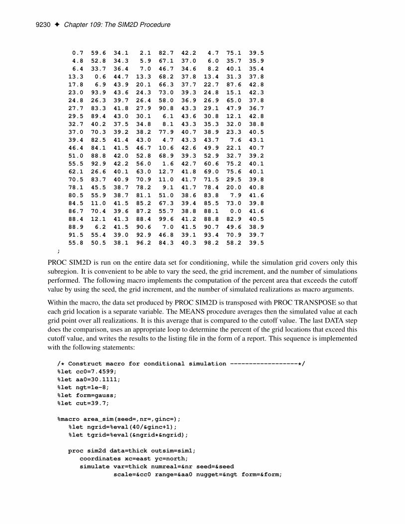
9230 F Chapter 109: The SIM2D Procedure
0.7 59.6 34.1 2.1 82.7 42.2 4.7 75.1 39.54.8 52.8 34.3 5.9 67.1 37.0 6.0 35.7 35.96.4 33.7 36.4 7.0 46.7 34.6 8.2 40.1 35.4
13.3 0.6 44.7 13.3 68.2 37.8 13.4 31.3 37.817.8 6.9 43.9 20.1 66.3 37.7 22.7 87.6 42.823.0 93.9 43.6 24.3 73.0 39.3 24.8 15.1 42.324.8 26.3 39.7 26.4 58.0 36.9 26.9 65.0 37.827.7 83.3 41.8 27.9 90.8 43.3 29.1 47.9 36.729.5 89.4 43.0 30.1 6.1 43.6 30.8 12.1 42.832.7 40.2 37.5 34.8 8.1 43.3 35.3 32.0 38.837.0 70.3 39.2 38.2 77.9 40.7 38.9 23.3 40.539.4 82.5 41.4 43.0 4.7 43.3 43.7 7.6 43.146.4 84.1 41.5 46.7 10.6 42.6 49.9 22.1 40.751.0 88.8 42.0 52.8 68.9 39.3 52.9 32.7 39.255.5 92.9 42.2 56.0 1.6 42.7 60.6 75.2 40.162.1 26.6 40.1 63.0 12.7 41.8 69.0 75.6 40.170.5 83.7 40.9 70.9 11.0 41.7 71.5 29.5 39.878.1 45.5 38.7 78.2 9.1 41.7 78.4 20.0 40.880.5 55.9 38.7 81.1 51.0 38.6 83.8 7.9 41.684.5 11.0 41.5 85.2 67.3 39.4 85.5 73.0 39.886.7 70.4 39.6 87.2 55.7 38.8 88.1 0.0 41.688.4 12.1 41.3 88.4 99.6 41.2 88.8 82.9 40.588.9 6.2 41.5 90.6 7.0 41.5 90.7 49.6 38.991.5 55.4 39.0 92.9 46.8 39.1 93.4 70.9 39.755.8 50.5 38.1 96.2 84.3 40.3 98.2 58.2 39.5
;
PROC SIM2D is run on the entire data set for conditioning, while the simulation grid covers only thissubregion. It is convenient to be able to vary the seed, the grid increment, and the number of simulationsperformed. The following macro implements the computation of the percent area that exceeds the cutoffvalue by using the seed, the grid increment, and the number of simulated realizations as macro arguments.
Within the macro, the data set produced by PROC SIM2D is transposed with PROC TRANSPOSE so thateach grid location is a separate variable. The MEANS procedure averages then the simulated value at eachgrid point over all realizations. It is this average that is compared to the cutoff value. The last DATA stepdoes the comparison, uses an appropriate loop to determine the percent of the grid locations that exceed thiscutoff value, and writes the results to the listing file in the form of a report. This sequence is implementedwith the following statements:
/* Construct macro for conditional simulation ------------------*/%let cc0=7.4599;%let aa0=30.1111;%let ngt=1e-8;%let form=gauss;%let cut=39.7;
%macro area_sim(seed=,nr=,ginc=);%let ngrid=%eval(40/&ginc+1);%let tgrid=%eval(&ngrid*&ngrid);
proc sim2d data=thick outsim=sim1;coordinates xc=east yc=north;simulate var=thick numreal=&nr seed=&seed
scale=&cc0 range=&aa0 nugget=&ngt form=&form;

Example 109.1: Simulation and Economic Feasibility F 9231
mean 40.1173;grid x=60 to 100 by &ginc
y= 0 to 40 by &ginc;run;
proc transpose data=sim1 out=sim2 prefix=sims;by _iter_;var svalue;
run;
proc means data=sim2 noprint n mean;var sims1-sims&tgrid;output out=msim n=numsim mean=ms1-ms&tgrid;
run;
data _null_;file print;array simss ms1-ms&tgrid;set msim;cflag=0;do ss=1 to &tgrid;
tempv=simss[ss];if simss[ss] > &cut then do;
cflag + 1;end;
end;
area_per=100*(cflag/&tgrid);put // +5 'Conditional Simulation of Coal Seam'
' Thickness for Subregion';put / +5 'Subregion is South-East Corner 40 by 40 distance units';put / +5 "Seed:&seed" +2 "Grid Increment:&ginc";put / +5 "Total Number of Grid Points:&tgrid" +2
"Number of Simulations:&nr";put / +5 "Percent of Subregion Exceeding Cutoff of %left(&cut) ft.:"
+2 area_per 5.2;run;
%mend area_sim;
In the following statement, you invoke the macro three times. Each time, the macro is invoked with a differentseed and combination of the grid increment and number of simulations. The macro is first invoked with arelatively coarse grid (grid increment of 10 distance units) and a small number of realizations (5). The outputof this conditional simulation is shown in Output 109.1.1.
/* Execute macro for coarse grid -------------------------------*/%area_sim(seed=12345,nr=5,ginc=10);

9232 F Chapter 109: The SIM2D Procedure
Output 109.1.1 Conditional Simulation of Coal Seam Thickness on a Coarse Grid
Simulating a Subregion for Economic Feasibility
Conditional Simulation of Coal Seam Thickness for Subregion
Subregion is South-East Corner 40 by 40 distance units
Seed:12345 Grid Increment:10
Total Number of Grid Points:25 Number of Simulations:5
Percent of Subregion Exceeding Cutoff of 39.7 ft.: 76.00
The next invocation, in the following statement, uses a finer grid and 50 realizations. The output of the secondconditional simulation is shown in Output 109.1.2.
/* Execute macro for fine grid and fewer simulations -----------*/%area_sim(seed=54321,nr=50,ginc=1);
Output 109.1.2 Conditional Simulation of Coal Seam Thickness on a Fine Grid
Simulating a Subregion for Economic Feasibility
Conditional Simulation of Coal Seam Thickness for Subregion
Subregion is South-East Corner 40 by 40 distance units
Seed:54321 Grid Increment:1
Total Number of Grid Points:1681 Number of Simulations:50
Percent of Subregion Exceeding Cutoff of 39.7 ft.: 76.09
The final invocation, in the following statement, uses the same grid increment and 500 realizations. Theoutput of this conditional simulation is shown in Output 109.1.3.
/* Execute macro for fine grid and more simulations ------------*/%area_sim(seed=655311,nr=500,ginc=1);

Example 109.2: Variability at Selected Locations F 9233
Output 109.1.3 Conditional Simulation of Coal Seam Thickness on a Fine Grid
Simulating a Subregion for Economic Feasibility
Conditional Simulation of Coal Seam Thickness for Subregion
Subregion is South-East Corner 40 by 40 distance units
Seed:655311 Grid Increment:1
Total Number of Grid Points:1681 Number of Simulations:500
Percent of Subregion Exceeding Cutoff of 39.7 ft.: 76.09
The results from the preceding simulations indicate that about 76% of the subregion exceeds the cutoff value.
NOTE: The number of grid points in the simulation increases with the square of the decrease in the gridincrement, leading to long CPU processing times. Increasing the number of realizations results in a linearincrease in processing times. Hence, using as coarse a grid as possible allows for more realizations andexperimentation with different seeds.
Example 109.2: Variability at Selected LocationsThis example exhibits a more detailed investigation of the variation of simulated Thick variable values. Youuse the same thick data set from the section “Getting Started: SIM2D Procedure” on page 9191, and you areinterested in the simulated values statistics at two selected grid points.
Specifically, you perform a simulation asking for 5,000 realizations (iterations) at two points of the regiondefined in the section “Preliminary Spatial Data Analysis” on page 9191. These are the extreme southwestpoint and a point toward the northeast corner of the region. Since you want to avoid performing the simulationacross the whole region, you need to produce a GDATA= data set to specify the coordinates of the selectedpoints. These steps are implemented using the following DATA step and statements:

9234 F Chapter 109: The SIM2D Procedure
title 'Investigation of Random Field Variability';
data thick;input East North Thick @@;label Thick='Coal Seam Thickness';datalines;0.7 59.6 34.1 2.1 82.7 42.2 4.7 75.1 39.54.8 52.8 34.3 5.9 67.1 37.0 6.0 35.7 35.96.4 33.7 36.4 7.0 46.7 34.6 8.2 40.1 35.4
13.3 0.6 44.7 13.3 68.2 37.8 13.4 31.3 37.817.8 6.9 43.9 20.1 66.3 37.7 22.7 87.6 42.823.0 93.9 43.6 24.3 73.0 39.3 24.8 15.1 42.324.8 26.3 39.7 26.4 58.0 36.9 26.9 65.0 37.827.7 83.3 41.8 27.9 90.8 43.3 29.1 47.9 36.729.5 89.4 43.0 30.1 6.1 43.6 30.8 12.1 42.832.7 40.2 37.5 34.8 8.1 43.3 35.3 32.0 38.837.0 70.3 39.2 38.2 77.9 40.7 38.9 23.3 40.539.4 82.5 41.4 43.0 4.7 43.3 43.7 7.6 43.146.4 84.1 41.5 46.7 10.6 42.6 49.9 22.1 40.751.0 88.8 42.0 52.8 68.9 39.3 52.9 32.7 39.255.5 92.9 42.2 56.0 1.6 42.7 60.6 75.2 40.162.1 26.6 40.1 63.0 12.7 41.8 69.0 75.6 40.170.5 83.7 40.9 70.9 11.0 41.7 71.5 29.5 39.878.1 45.5 38.7 78.2 9.1 41.7 78.4 20.0 40.880.5 55.9 38.7 81.1 51.0 38.6 83.8 7.9 41.684.5 11.0 41.5 85.2 67.3 39.4 85.5 73.0 39.886.7 70.4 39.6 87.2 55.7 38.8 88.1 0.0 41.688.4 12.1 41.3 88.4 99.6 41.2 88.8 82.9 40.588.9 6.2 41.5 90.6 7.0 41.5 90.7 49.6 38.991.5 55.4 39.0 92.9 46.8 39.1 93.4 70.9 39.755.8 50.5 38.1 96.2 84.3 40.3 98.2 58.2 39.5
;
data grid;input xc yc;datalines;0 075 75
;
Then, you run PROC SIM2D with the same parameters and characteristics as those shown in the section“Preliminary Spatial Data Analysis” on page 9191. This time, however, you ask for simulated values only atthe two locations you specified in the previous DATA step. The following statements execute the requestedsimulation:
proc sim2d data=thick outsim=sim1;coordinates xc=East yc=North;simulate var=Thick numreal=5000 seed=79931
scale=7.4599 range=30.1111 form=gauss;mean 40.1173;grid gdata=grid xc=xc yc=yc;
run;
After the simulation is performed, summary statistics are computed for each of the specified grid points.

Example 109.2: Variability at Selected Locations F 9235
In particular, you use PROC UNIVARIATE and a BY statement to request the quantiles and the extremeobservations at these locations, as the following statements show:
proc sort data=sim1;by gxc gyc;
run;
proc univariate data=sim1;var svalue;by gxc gyc;ods select Quantiles ExtremeObs;title 'Simulation Statistics at Selected Grid Points';
run;
The summary statistics for the first grid point (East=0, North=0) are presented in Output 109.2.1.
Output 109.2.1 Simulation Statistics at Grid Point (East=0, North=0)
Simulation Statistics at Selected Grid Points
The UNIVARIATE ProcedureVariable: SVALUE (Simulated Value at Grid Point)
X-coordinate of the grid point=0 Y-coordinate of the grid point=0
Quantiles (Definition 5)
Level Quantile
100% Max 42.4207
99% 41.8960
95% 41.5315
90% 41.3419
75% Q3 41.0324
50% Median 40.6701
25% Q1 40.2871
10% 39.9904
5% 39.7825
1% 39.4181
0% Min 38.6864
X-coordinate of the grid point=0 Y-coordinate of the grid point=0
Extreme Observations
Lowest Highest
Value Obs Value Obs
38.6864 2691 42.2952 1149
38.8611 1817 42.3114 3612
38.9013 3026 42.3305 3757
38.9467 2275 42.4177 135
38.9823 3100 42.4207 4536
Finally, Output 109.2.2 displays the summary statistics for the second grid point (East=75, North=75).

9236 F Chapter 109: The SIM2D Procedure
Output 109.2.2 Simulation Statistics at Grid Point (East=75, North=75)
Simulation Statistics at Selected Grid Points
The UNIVARIATE ProcedureVariable: SVALUE (Simulated Value at Grid Point)
X-coordinate of the grid point=75 Y-coordinate of the grid point=75
Quantiles (Definition 5)
Level Quantile
100% Max 40.1171
99% 40.1147
95% 40.1131
90% 40.1122
75% Q3 40.1108
50% Median 40.1092
25% Q1 40.1075
10% 40.1062
5% 40.1053
1% 40.1035
0% Min 40.1001
X-coordinate of the grid point=75 Y-coordinate of the grid point=75
Extreme Observations
Lowest Highest
Value Obs Value Obs
40.1001 7176 40.1167 8980
40.1007 6262 40.1167 9272
40.1011 7383 40.1169 5676
40.1016 7156 40.1170 6514
40.1017 5643 40.1171 5329
For each simulation location, a single realization might result in values that differ significantly from therandom field mean at that location. However, the averages of progressively larger numbers of realizationstend to shorten this gap and reduce the simulation variability, as exhibited in the results for the two examplelocations in Output 109.2.1 and Output 109.2.2. At the limit of an infinite number of realizations, thesimulation mean recovers the mean and covariance structure of the random field.

Example 109.3: Risk Analysis with Simulation F 9237
Example 109.3: Risk Analysis with SimulationThis example is in the field of environmental risk assessment. A square region of size 500 km � 500 kmhas been sampled for arsenic in drinking water. The logAsData data set consists of 138 simulated arseniclogarithm concentration observations represented by the logAs variable. Section “Example 128.1: Aspectsof Semivariogram Model Fitting” on page 10711 in Chapter 128, “The VARIOGRAM Procedure,” treatsthese observations as actual data in order to determine the spatial continuity structure for illustration in theexamples.
A preliminary analysis indicates that the population exposure to the pollutant is currently at a relatively lowlevel, as shown in the section “Example 71.1: Spatial Prediction of Pollutant Concentration” on page 5418 inChapter 71, “The KRIGE2D Procedure,” procedure. In particular, spatial prediction with kriging suggeststhat less than 1% of the region is affected by arsenic concentration in water that exceeds the World HealthOrganization (WHO) standard of 10 �g/lt.
You want to simulate the random field of the arsenic logarithm concentration so that you can gain insightinto the characteristics of this field. Your objective is to assess whether the occurrence of above-thresholdarsenic concentrations is a localized phenomenon, and whether you might expect more such occurrencesacross the region. For the simulation you need the outcome of the spatial continuity analysis in section “Ex-ample 128.1: Aspects of Semivariogram Model Fitting” on page 10711 in Chapter 128, “The VARIOGRAMProcedure.” These results are the fitted semivariance models that are stored in the SemivAsStore item storeby PROC VARIOGRAM.
Based on the discussion in the section “Example 109.1: Simulation and Economic Feasibility” on page 9228,you simulate the arsenic logarithm concentration on the premise of the ergodicity assumption. In brief, thisassumption relates the mean and covariances of each individual realization to the corresponding values ofthe random field; see also the section “Ergodicity” on page 10679 in Chapter 128, “The VARIOGRAMProcedure.” In the present case you are interested in the average of a large size of realizations, rather thanindividual ones. A single realization could suggest possible locations where the WHO regulatory standardmight be violated. The average of multiple realizations has a smoothing effect on individual excessive-concentration episodes in single realizations. The smoothing enables you to see general characteristics of thearsenic concentration field behavior on the basis of its spatial correlation description.
For illustration, assume a rectangular grid of nodes with an equal spacing of 10 km between neighboringnodes in the north and east directions. Then, simulated values are produced at a total of 51 � 51 D 2601
locations.
You begin by reading the logAsData data set with the following DATA step:

9238 F Chapter 109: The SIM2D Procedure
title 'Risk Assessment with Simulation';
data logAsData;input East North logAs @@;label logAs='log(As) Concentration';datalines;193.0 296.6 -0.68153 232.6 479.1 0.96279 268.7 312.5 -1.0290843.6 4.9 0.65010 152.6 54.9 1.87076 449.1 395.8 0.95932
310.9 493.6 -1.66208 287.8 164.9 -0.01779 330.0 8.0 2.06837225.7 241.7 0.15899 452.3 83.4 -1.21217 156.5 462.5 -0.8903111.5 84.4 -0.24496 144.4 335.7 0.11950 149.0 431.8 -0.57251
234.3 123.2 -1.33642 37.8 197.8 -0.27624 183.1 173.9 -2.14558149.3 426.7 -1.06506 434.4 67.5 -1.04657 439.6 237.0 -0.0907436.4 175.2 -1.21211 370.6 244.0 3.28091 452.0 96.5 -0.77081
247.0 86.8 0.04720 413.6 373.2 1.78235 253.5 291.7 0.56132129.7 111.9 1.34000 352.7 42.1 0.23621 279.3 82.7 2.12350382.6 290.7 0.86756 188.2 222.8 -1.23308 382.8 154.5 -0.94094304.4 309.2 -1.95158 337.5 387.2 -1.31294 490.7 189.8 0.40206159.0 100.1 -0.22272 245.5 329.2 -0.26082 372.1 379.5 -1.89078417.8 84.1 -1.25176 173.9 407.6 -0.24240 121.5 107.7 1.54509453.5 313.6 0.65895 143.5 346.7 -0.87196 157.4 125.5 -1.96165371.8 353.2 -0.59464 358.9 338.2 -1.07133 8.6 437.8 1.44203395.9 394.2 -0.24144 149.5 58.9 1.17459 453.5 420.6 -0.63951182.3 85.0 1.00005 21.0 290.1 0.31016 11.1 352.2 -0.88418131.2 238.4 -0.57184 104.9 6.3 1.12054 247.3 256.0 0.14019428.4 383.7 0.92448 327.8 481.1 -2.72543 199.2 92.8 -0.05717453.9 230.1 0.16571 205.0 250.6 0.07581 459.5 271.6 0.93700229.5 262.8 1.83590 370.4 228.6 2.96611 330.2 281.9 1.79723354.8 388.3 -3.18262 406.2 222.7 2.41594 254.4 393.1 2.0322196.7 85.2 -0.47156 407.2 256.8 0.66747 498.5 273.8 1.03041
417.2 471.4 -1.42766 368.8 424.3 -0.70506 303.0 59.1 1.43070403.1 264.1 1.64554 21.2 360.8 0.67094 148.2 78.1 2.15323305.5 310.7 -1.47985 228.5 180.3 -0.68386 161.1 143.3 1.0790170.5 155.1 0.54652 363.1 282.6 -0.43051 86.0 472.5 -1.18855
175.9 105.3 -2.08112 96.8 426.3 1.56592 475.1 453.1 -1.53776125.7 485.4 1.40054 277.9 201.6 -0.54565 406.2 125.0 -1.3865760.0 275.5 -0.59966 431.3 494.6 -0.36860 399.9 399.0 -0.7726528.8 311.1 0.91693 166.1 348.2 -0.49056 266.6 83.5 0.6727754.7 356.3 0.49596 433.5 460.3 -1.61309 201.7 167.6 -1.40678
158.1 203.6 -1.32499 67.6 230.4 1.14672 81.9 250.0 0.63378372.0 50.7 0.72445 26.4 264.6 1.00862 300.1 91.7 -0.74089303.0 447.4 1.74589 108.4 386.2 1.12847 55.6 191.7 0.9517536.3 273.2 1.78880 94.5 298.3 -2.43320 366.1 187.3 -0.80526
130.7 389.2 -0.31513 37.2 324.2 0.24489 295.5 211.8 0.4189958.6 206.2 0.18495 346.3 142.8 -0.92038 484.2 215.9 0.08012
451.4 415.7 0.02773 58.9 86.5 0.17652 212.6 363.9 0.17215378.7 407.6 0.51516 265.9 305.0 -0.30718 123.2 314.8 -0.9059126.9 471.7 1.70285 16.5 7.1 0.51736 255.1 472.6 2.02381
111.5 148.4 -0.09658 440.4 375.0 1.23285 406.4 19.5 1.01181321.2 65.8 -0.02095 466.4 357.1 -0.49272 2.0 484.6 0.50994200.9 205.1 0.43543 30.3 337.0 1.60882 297.0 12.7 1.79824158.2 450.7 0.05295 122.8 105.3 1.53936 417.8 329.7 -2.08124
;

Example 109.3: Risk Analysis with Simulation F 9239
For this simulation you use the spatial correlation information that is saved in the SemivAsStore item store inthe section “Example 128.1: Aspects of Semivariogram Model Fitting” on page 10711 in Chapter 128, “TheVARIOGRAM Procedure,” with the following statements:
ods graphics on;
proc variogram data=logAsData plots=none;store out=SemivAsStore / label='LogAs Concentration Models';compute lagd=5 maxlag=40;coord xc=East yc=North;model form=auto(mlist=(exp,gau,mat) nest=1 to 2);var logAs;
run;
In PROC SIM2D you specify the container item store with the IN= option of the RESTORE statement. Yourequest correlation input from an item store by specifying the STORESELECT option in the SIMULATEstatement. You request 5,000 realizations for this simulation by specifying the number in the NUMREAL=option of the SIMULATE statement.
Assume that you first want to review the saved models in the item store. Use the INFO option of theRESTORE statement to produce a table with information about the top-ranking fitted model in the item store.Use the DET and ONLY suboptions of the INFO option to request details about all fitted models included inthe item store. The ONLY suboption suppresses the simulation tasks and produces only the tables about theitem store. You specify the following statements:
proc sim2d data=logAsData outsim=Outsim plots=none;restore in=SemivAsStore / info(det only);coordinates xc=East yc=North;simulate var=logAs numreal=5000 storeselect seed=39841;grid x=0 to 500 by 10 y=0 to 500 by 10;
run;
PROC SIM2D produces a table with general information about the input item store identity, as shown inOutput 109.3.1.
Output 109.3.1 PROC SIM2D and Input Item Store General Information
Risk Assessment with Simulation
The SIM2D Procedure
Correlation Model Item Store Information
Input Item Store WORK.SEMIVASSTORE
Item Store Label LogAs Concentration Models
Data Set Created From WORK.LOGASDATA
By-group Information No By-groups Present
Created By PROC VARIOGRAM
Date Created 16OCT18:01:05:24

9240 F Chapter 109: The SIM2D Procedure
Output 109.3.2 displays the item store variables, in addition to the mean and standard deviation of theirdata set of origin. In this case, the logAs values come from the logAsData data set. By default, the SIM2Dprocedure uses the variable mean in the item store for the simulation, unless you explicitly specify the MEANstatement.
Output 109.3.2 Variables in the Input Item Store
Item Store Variables
Variable MeanStd
Deviation
logAs 0.084309 1.527707
The models in the SemivAsStore item store that have been fitted to the arsenic logarithm logAs empiricalsemivariance are shown in Output 109.3.3. The default item store model selection is the model on top of thelist in Output 109.3.3.
Output 109.3.3 Angle and Models Information in the Input Item Store
Item StoreModels For
logAs
Class Model
1 Gau-Gau
Gau-Mat
Mat-Mat
2 Exp-Gau
3 Exp-Mat
4 Mat
5 Gau
6 Exp
Exp-Exp
Mat-Exp
Gau-Exp
You run again the SIM2D procedure without the INFO option in the RESTORE statement. This action promptsPROC SIM2D to run the simulation tasks that you specify with the SIMULATE statement. You specify theSTORESELECT option in the SIMULATE statement without any suboptions, so that the simulation uses thedefault model selection in the SemivAsStore item store. You save the simulation output in the Outsim outputdata set. You also specify the SIM and the SEMIVAR suboptions in the PLOTS option of the PROC SIM2Dstatement to obtain output plots. You use the following statements:
proc sim2d data=logAsData outsim=Outsim plots=(sim semivar);restore in=SemivAsStore;coordinates xc=East yc=North;simulate var=logAs numreal=5000 storeselect seed=89702;grid x=0 to 500 by 10 y=0 to 500 by 10;
run;

Example 109.3: Risk Analysis with Simulation F 9241
NOTE: This step can take several minutes to run, and it produces a data set with over 10 million observations.When you run these statements, PROC SIM2D again produces a table about the input item store identity.This output is followed by a number of observations table and information about the simulation task, asshown in Output 109.3.4.
Output 109.3.4 Number of Observations and Simulation Information Tables
Risk Assessment with Simulation
The SIM2D Procedure
Simulation: SIM1, Dependent Variable: logAs
Number of Observations Read 138
Number of Observations Used 138
Simulation Information
Simulation Grid Points 2601
Type Conditional
Number of Realizations 5000
The SIM2D procedure uses the selected fitted Gaussian-Gaussian model in the SemivAsStore item store.Output 109.3.5 shows the saved parameter values of the model that are used in the simulation.
Output 109.3.5 Information about the Gaussian-Gaussian Model
Covariance Model Information
Nested Structure 1 Type Gaussian
Nested Structure 1 Sill 0.3276647
Nested Structure 1 Range 62.312823
Nested Structure 1 Effective Range 107.92898
Nested Structure 2 Type Gaussian
Nested Structure 2 Sill 1.2615457
Nested Structure 2 Range 21.459553
Nested Structure 2 Effective Range 37.169036
Nugget Effect 0.0830751
Output 109.3.6 shows a plot of the correlation model used in the simulation. Its parameters come from thestored information in the SemivAsStore item store.

9242 F Chapter 109: The SIM2D Procedure
Output 109.3.6 Gaussian-Gaussian Semivariogram Model Used in Simulation
The PLOTS=SIM option produces contours of the mean value of the 5,000 realizations for each one of theoutput grid locations, and a surface of the associated standard deviation. The resulting plot is shown inOutput 109.3.7. The mean value contours exhibit reduced variation compared to a SIM plot of one singlerealization. In fact, Output 109.3.7 is very similar to the prediction plot of the same Gaussian model in thesection “Example 71.1: Spatial Prediction of Pollutant Concentration” on page 5418 in Chapter 71, “TheKRIGE2D Procedure.”
Clearly, there appears to be a small area of increased arsenic concentration values, which is located inthe central-eastern part of the domain. The WHO threshold of 10 �g/lt for the maximum allowed arsenicconcentration in water translates into about 2.3 in the log scale. The indicated area is the only one within theregion where the simulated means exceed the value 3. In addition, there appear to be two smaller areas ofsimulated means values at or above 2 in the southern part of the region.

Example 109.3: Risk Analysis with Simulation F 9243
Output 109.3.7 Simulated Arsenic Logarithm Values with Gaussian-Gaussian Covariance
The simulation plot indicates that arsenic concentration values in excess of the WHO health standardis a rather localized phenomenon. If it were not so, then the plot would suggest that increased arsenicconcentrations extend across larger areas. In turn, this means that individual realizations would tend toproduce systematically higher arsenic concentrations at different neighboring locations, and their averagewould appear as higher logAs values in the SIM plot. Instead, you conclude that the Gaussian-Gaussiancorrelation that describes the spatial continuity for the arsenic logarithm observations leads to only localizedoccurrence of the WHO standard violation.
Now you want to find out whether additional localized occurrences might take place on the basis of theGaussian-Gaussian spatial continuity behavior. The distribution of the simulation standard deviation valuesin Output 109.3.7 offers important feedback about this issue. Observe the areas in the plot where the meansgradient indicates increasing values. The means contours create several pools where the values increase tosimulated means higher than 1.
With the clear exceptions of the isolated area in the central-eastern part of the domain and the pool in thesouth-west that exhibit logAs values above 2, the simulation standard deviation seems to be around 1 or lessin almost all other pools with logAs values above 1. Due to those relatively low standard deviations, thisvisual inspection suggests that even in individual realizations you might rarely expect the arsenic logarithmto exceed the threshold value of around 2.3.

9244 F Chapter 109: The SIM2D Procedure
However, in the few pools of logAs values above 1, there can be patches of increased standard deviation. Inthese cases, you suspect that arsenic concentration could exceed occasionally the WHO regulatory standard,even if the plot of the simulated means does not explicitly portray so.
Based on these remarks, you want to quantify the percentage of the region that could be affected by excessivearsenic concentration. You begin with a DATA step that takes as input the simulation Outsim output dataset. The DATA step marks the simulated arsenic logarithm means values that are in excess of the WHOconcentration threshold of 10 �g/lt, and saves the outcome into an indicator variable OverLimit. At the sametime, the arsenic logarithm values are transformed back into arsenic concentration values so that they can becompared to the threshold value. The simulated means in the Outsim data set are stored in the svalue variable.You use the following statements:
data AsOverLimit;set Outsim;OverLimit = (exp(svalue) > 10) * 100;
run;
Then, you use the MEANS procedure to express the selected nodes population (where the WHO standardviolation occurs) as a percentage of the entire domain area. You invoke PROC MEANS twice. The first time,you average over each realization in the PROC SIM2D output. For that purpose, you use the variable _ITER_in the simulation sim1 output data set as a BY variable in PROC MEANS. You save the iteration-averagedindicator values in the PctOverLimit variable. The second time, PROC MEANS averages the PctOverLimitvariable to obtain the percentage you want. You also specify the P5 and P95 options in the PROC MEANSstatement to request the lower and upper confidence limits, respectively, in this computation. The intervalbetween those limits expresses the 90% interval for the true area percentage based on the stochastic simulation.You use the following statements:
proc means data=AsOverLimit noprint;by _ITER_;var OverLimit;output out=OverLimitData mean=PctOverLimit;
run;proc means data=OverLimitData mean p5 p95;
var PctOverLimit;label PctOverLimit="Percent above threshold";
run;
The result is shown in Output 109.3.8. PROC MEANS accounts for all individual occurrences throughoutthe simulation where the WHO arsenic concentration threshold is exceeded. This happens at about 3.9%of the total area in 5,000 realizations. Compare this value to the less than 1% percentage in the PROCKRIGE2D prediction, as reported in the beginning of this section. On one hand, the prediction outcome tellsyou what goes on currently across the region within a degree of certainty given by the prediction error. Onthe other hand, the simulation provides you with an indicator that under the given spatial continuity estimatea relatively larger area is in potential danger of being affected by above-threshold arsenic concentration.
In fact, the 5% and 95% confidence limits in Output 109.3.8 show the area percentage limits within whichyou can expect excessive arsenic concentration. Based on the stochastic simulation, at the 90% confidencelevel the arsenic concentration in drinking water is expected to violate the WHO regulatory standard inanywhere from about 2.6% to 5.4% of the study region.
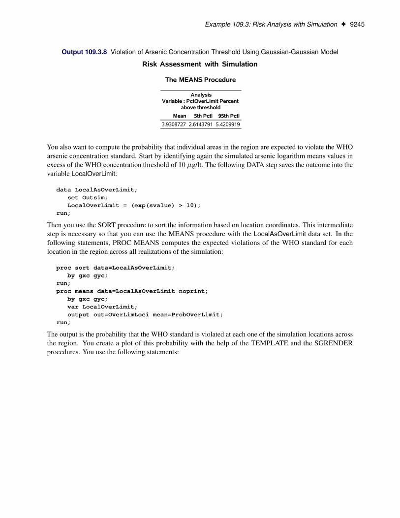
Example 109.3: Risk Analysis with Simulation F 9245
Output 109.3.8 Violation of Arsenic Concentration Threshold Using Gaussian-Gaussian Model
Risk Assessment with Simulation
The MEANS Procedure
AnalysisVariable : PctOverLimit Percent
above threshold
Mean 5th Pctl 95th Pctl
3.9308727 2.6143791 5.4209919
You also want to compute the probability that individual areas in the region are expected to violate the WHOarsenic concentration standard. Start by identifying again the simulated arsenic logarithm means values inexcess of the WHO concentration threshold of 10 �g/lt. The following DATA step saves the outcome into thevariable LocalOverLimit:
data LocalAsOverLimit;set Outsim;LocalOverLimit = (exp(svalue) > 10);
run;
Then you use the SORT procedure to sort the information based on location coordinates. This intermediatestep is necessary so that you can use the MEANS procedure with the LocalAsOverLimit data set. In thefollowing statements, PROC MEANS computes the expected violations of the WHO standard for eachlocation in the region across all realizations of the simulation:
proc sort data=LocalAsOverLimit;by gxc gyc;
run;proc means data=LocalAsOverLimit noprint;
by gxc gyc;var LocalOverLimit;output out=OverLimLoci mean=ProbOverLimit;
run;
The output is the probability that the WHO standard is violated at each one of the simulation locations acrossthe region. You create a plot of this probability with the help of the TEMPLATE and the SGRENDERprocedures. You use the following statements:

9246 F Chapter 109: The SIM2D Procedure
proc template;define statgraph surfacePlot;
dynamic _VARX _VARY _VAR _TITLE _LEGENDLABEL;BeginGraph;entrytitle _TITLE;layout overlay /
xaxisopts = (offsetmax=0)yaxisopts = (offsetmax=0);contourplotparm x=_VARX y=_VARY z=_VAR /
nhint=10 name='probplot';continuouslegend 'probplot' / title=_LEGENDLABEL;
endlayout;EndGraph;
end;run;
proc sgrender data=OverLimLoci template=surfacePlot;dynamic _VARX ='gxc'
_VARY ='gyc'_VAR ='ProbOverLimit'_TITLE='Arsenic WHO Standard Violation'_LEGENDLABEL='Violation Probability';
label gyc='North' gxc='East';run;
ods graphics off;
Output 109.3.9 shows the map of probability that the arsenic concentration WHO standard is violated inthe region for the selected spatial correlation model of the pollutant. Based on the preceding analysis, theprobability is very close to 1 in the area where the simulation mean values are above the standard limit. Afew more areas that were indicated earlier in the analysis suggest a violation probability between 20% and40%. The remaining areas in the region exhibit very low probability, which is notably nonzero at a fewscattered locations. These findings suggest that throughout the simulation there have been realizations wherethe arsenic WHO standard was exceeded at locations whose simulated mean is well below that standard.
From the environmental risk assessment perspective, the preceding analysis can trigger a more detailedinvestigation into areas in the region where the health standard might be violated. Although the originalobservations in the logAsData data set indicate no existing problem in some of these areas, the presentexample illustrates that spatial analysis and simulation can raise flags of caution. This type of analysis canhelp to focus scientific, management, and policy efforts on these particular areas of the region and to monitorclosely the pollutant concentration for potential health risks.
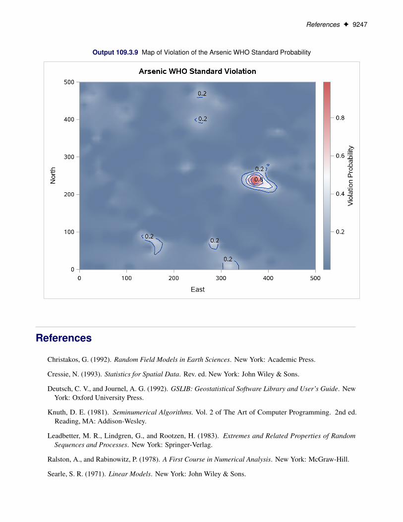
References F 9247
Output 109.3.9 Map of Violation of the Arsenic WHO Standard Probability
References
Christakos, G. (1992). Random Field Models in Earth Sciences. New York: Academic Press.
Cressie, N. (1993). Statistics for Spatial Data. Rev. ed. New York: John Wiley & Sons.
Deutsch, C. V., and Journel, A. G. (1992). GSLIB: Geostatistical Software Library and User’s Guide. NewYork: Oxford University Press.
Knuth, D. E. (1981). Seminumerical Algorithms. Vol. 2 of The Art of Computer Programming. 2nd ed.Reading, MA: Addison-Wesley.
Leadbetter, M. R., Lindgren, G., and Rootzen, H. (1983). Extremes and Related Properties of RandomSequences and Processes. New York: Springer-Verlag.
Ralston, A., and Rabinowitz, P. (1978). A First Course in Numerical Analysis. New York: McGraw-Hill.
Searle, S. R. (1971). Linear Models. New York: John Wiley & Sons.

Subject Index
computational detailsSIM2D procedure, 9225
conditional and unconditional simulationSIM2D procedure, 9190
conditional distributions of multivariate normalrandom variables
SIM2D procedure, 9223covariance matrix
symmetric and positive definite (SIM2D), 9222cubic semivariance model
SIM2D procedure, 9213
exponential semivariance modelSIM2D procedure, 9213
Gaussian assumptionSIM2D procedure, 9190
Gaussian random fieldSIM2D procedure, 9190
Gaussian semivariance modelSIM2D procedure, 9213
Matérn semivariance modelSIM2D procedure, 9213
memory usageSIM2D procedure, 9225
nugget effectSIM2D procedure, 9215
ODS graph namesSIM2D procedure, 9228
ODS GraphicsSIM2D procedure, 9201
ODS table namesSIM2D procedure, 9227
output data setsSIM2D procedure, 9201, 9225, 9226
OUTSIM= data setSIM2D procedure, 9225, 9226
pentaspherical semivariance modelSIM2D procedure, 9213
plots (SIM2D procedure)Observations, 9228Semivariogram, 9228Simulation, 9228
SIM2D procedure
Cholesky root, 9222computational details, 9225conditional and unconditional simulation, 9190conditional distributions of multivariate normal
random variables, 9223conditional simulation, 9190, 9223cubic semivariance model, 9213examples, 9191, 9228, 9233, 9237exponential semivariance model, 9213Gaussian assumption, 9190Gaussian random field, 9190Gaussian semivariance model, 9213LU decomposition, 9222Matérn semivariance model, 9213memory usage, 9225nugget effect, 9215ODS graph names, 9228ODS Graphics, 9201ODS table names, 9227output data sets, 9201, 9225, 9226OUTSIM= data set, 9225, 9226pentaspherical semivariance model, 9213quadratic form, 9223simulation of spatial random fields, 9222–9225sine hole effect semivariance model, 9213spherical semivariance model, 9213unconditional simulation, 9190, 9223
SIM2D procedure, plotsObservations, 9228Semivariogram, 9228Simulation, 9228
SIM2D procedure, tablesModel Information, 9227Number of Observations, 9226Simulation Information, 9227Store Information, 9210, 9227, 9239Store Model Information, 9210, 9227, 9240Store Variables Information, 9210, 9227, 9240
simulationat individual locations (SIM2D), 9207conditional (SIM2D), 9190, 9223correlation model (SIM2D), 9191, 9194, 9212,
9239on one-dimensional grid (SIM2D), 9207unconditional (SIM2D), 9190, 9223
simulation of spatial random fieldsSIM2D procedure, 9222–9225
sine hole effect semivariance model

SIM2D procedure, 9213spherical semivariance model
SIM2D procedure, 9213symmetric and positive definite (SIM2D)
covariance matrix, 9222
tables (SIM2D procedure)Model Information, 9227Number of Observations, 9226Simulation Information, 9227Store Information, 9210, 9227, 9239Store Model Information, 9210, 9227, 9240Store Variables Information, 9210, 9227, 9240

Syntax Index
ANGLE= optionSIMULATE statement (SIM2D), 9213
BY statementSIM2D procedure, 9205
COORDINATES statementSIM2D procedure, 9206
DATA= optionPROC SIM2D statement, 9200
FORM= optionSIMULATE statement (SIM2D), 9213
GRID statementSIM2D procedure, 9207
GRIDDATA= optionGRID statement (SIM2D), 9208
ID statementSIM2D procedure, 9209
IDGLOBAL optionPROC SIM2D statement, 9200
IDNUM optionPROC SIM2D statement, 9200
INFO DETAILS optionRESTORE statement (SIM2D), 9210
INFO ONLY optionRESTORE statement (SIM2D), 9210
INFO optionRESTORE statement (SIM2D), 9210
LABEL= optionGRID statement (SIM2D), 9209
MDATA= optionSIMULATE statement (SIM2D), 9214
MEAN statementSIM2D procedure, 9220
NARROW optionPROC SIM2D statement, 9200
NOPRINT optionPROC SIM2D statement, 9201
NPTS= optionGRID statement (SIM2D), 9207
NUGGET= optionSIMULATE statement (SIM2D), 9215
NUMREAL= option
SIMULATE statement (SIM2D), 9212
OUTSIM= optionPROC SIM2D statement, 9201
PLOTS optionSIM2D procedure, PROC SIM2D statement, 9201
PLOTS(ONLY) optionSIM2D procedure, PROC SIM2D statement, 9201
PLOTS=ALL optionSIM2D procedure, PROC SIM2D statement, 9201
PLOTS=EQUATE optionSIM2D procedure, PROC SIM2D statement, 9201
PLOTS=NONE optionSIM2D procedure, PROC SIM2D statement, 9202
PLOTS=OBSERVATIONS optionSIM2D procedure, PROC SIM2D statement, 9202
PLOTS=SEMIVARIOGRAM optionSIM2D procedure, PROC SIM2D statement, 9205
PLOTS=SIM optionSIM2D procedure, PROC SIM2D statement, 9203
PROC SIM2D statement, see SIM2D procedure
RANGE= optionSIMULATE statement (SIM2D), 9215
RATIO= optionSIMULATE statement (SIM2D), 9216
RESTORE statement (SIM2D), 9210
SCALE= optionSIMULATE statement (SIM2D), 9216
SEED= optionSIMULATE statement (SIM2D), 9216
SIM2D procedure, 9190syntax, 9198
SIM2D procedure, BY statement, 9205SIM2D procedure, COORDINATES statement, 9206
XCOORD= option, 9206YCOORD= option, 9206
SIM2D procedure, GRID statement, 9207GRIDDATA= option, 9208LABEL= option, 9209NPTS= option, 9207X= option, 9207XCCORD= option, 9208Y= option, 9207YCOORD= option, 9208
SIM2D procedure, ID statement, 9209SIM2D procedure, MEAN statement, 9220

SIM2D procedure, PROC SIM2D statement, 9200DATA= option, 9200IDGLOBAL option, 9200IDNUM option, 9200NARROW option, 9200NOPRINT option, 9201OUTSIM= option, 9201PLOTS option, 9201PLOTS(ONLY) option, 9201PLOTS=ALL option, 9201PLOTS=EQUATE option, 9201PLOTS=NONE option, 9202PLOTS=OBSERVATIONS option, 9202PLOTS=SEMIVARIOGRAM option, 9205PLOTS=SIM option, 9203
SIM2D procedure, RESTORE statement, 9210INFO DETAILS option, 9210INFO ONLY option, 9210INFO options, 9210
SIM2D procedure, SIMULATE statement, 9211ANGLE= option, 9213FORM= option, 9213MDATA= option, 9214NUGGET= option, 9215NUMREAL= option, 9212RANGE= option, 9215RATIO= option, 9216SCALE= option, 9216SEED= option, 9216SINGULAR= option, 9216SMOOTH= option, 9216STORESELECT ANGLEID= option, 9218STORESELECT MODEL= option, 9218STORESELECT option, 9216STORESELECT SVAR= option, 9219STORESELECT TYPE= option, 9216VAR= option, 9212
SIMULATE statement (SIM2D), 9211SINGULAR= option
SIMULATE statement (SIM2D), 9216SMOOTH= option
SIMULATE statement (SIM2D), 9216STORESELECT ANGLEID= option
SIMULATE statement (SIM2D), 9218STORESELECT MODEL= option
SIMULATE statement (SIM2D), 9218STORESELECT option
SIMULATE statement (SIM2D), 9216STORESELECT SVAR= option
SIMULATE statement (SIM2D), 9219STORESELECT TYPE= option
SIMULATE statement (SIM2D), 9216
VAR= option
SIMULATE statement (SIM2D), 9212
X= optionGRID statement (SIM2D), 9207
XCOORD= optionCOORDINATES statement (SIM2D), 9206GRID statement (SIM2D), 9208
Y= optionGRID statement (SIM2D), 9207
YCOORD= optionCOORDINATES statement (SIM2D), 9206GRID statement (SIM2D), 9208