satellite orbits, coverage, and antenna alignment

Telecommunications Satellite Communications

Satellite Orbits, Coverage, and Antenna Alignment

Courseware Sample87768-F0

Order no.: 87768-10 First Edition Revision level: 04/2016

By the staff of Festo Didactic

© Festo Didactic Ltée/Ltd, Quebec, Canada 2011 Internet: www.festo-didactic.com e-mail: [email protected]

Printed in Canada All rights reserved ISBN 978-2-89640-473-5 (Printed version) Legal Deposit – Bibliothèque et Archives nationales du Québec, 2011 Legal Deposit – Library and Archives Canada, 2011

The purchaser shall receive a single right of use which is non-exclusive, non-time-limited and limited geographically to use at the purchaser's site/location as follows.

The purchaser shall be entitled to use the work to train his/her staff at the purchaser’s site/location and shall also be entitled to use parts of the copyright material as the basis for the production of his/her own training documentation for the training of his/her staff at the purchaser’s site/location with acknowledgement of source and to make copies for this purpose. In the case of schools/technical colleges, training centers, and universities, the right of use shall also include use by school and college students and trainees at the purchaser’s site/location for teaching purposes.

The right of use shall in all cases exclude the right to publish the copyright material or to make this available for use on intranet, Internet and LMS platforms and databases such as Moodle, which allow access by a wide variety of users, including those outside of the purchaser’s site/location.

Entitlement to other rights relating to reproductions, copies, adaptations, translations, microfilming and transfer to and storage and processing in electronic systems, no matter whether in whole or in part, shall require the prior consent of Festo Didactic.

Information in this document is subject to change without notice and does not represent a commitment on the part of Festo Didactic. The Festo materials described in this document are furnished under a license agreement or a nondisclosure agreement.

Festo Didactic recognizes product names as trademarks or registered trademarks of their respective holders.

All other trademarks are the property of their respective owners. Other trademarks and trade names may be used in this document to refer to either the entity claiming the marks and names or their products. Festo Didactic disclaims any proprietary interest in trademarks and trade names other than its own.

© Festo Didactic 87768-10 III

Safety and Common Symbols

Caution, risk of danger

Safety and Common Symbols

IV © Festo Didactic 87768-10

© Festo Didactic 87768-10 V

Table of Contents

Preface .................................................................................................................. IX

About This Manual ................................................................................................ XI

List of Equipment Required ................................................................................. XIII

To the Instructor .................................................................................................. XV

Introduction Satellite Orbits, Coverage and Antenna Alignment .................. 1

DISCUSSION OF FUNDAMENTALS ....................................................... 1Satellite technology .................................................................. 1Understanding orbits ................................................................ 1Why study orbital mechanics and satellite coverage? ............. 2Earth-station antennas ............................................................. 3The LVSAT Orbit Simulator ..................................................... 4Exercises in this manual .......................................................... 9

Exercise 1 Orbital Mechanics ....................................................................... 11

DISCUSSION ................................................................................... 11Orbital mechanics .................................................................. 11Physical laws .......................................................................... 12

Simplifying assumptions ........................................................... 12Kepler’s laws as they apply to satellites ................................... 12Newton’s laws of motion ........................................................... 14Vectors and scalars .................................................................. 14Newton’s law of universal gravitation ........................................ 16

The ellipse .............................................................................. 16Reference frames and coordinate systems ........................... 18

Inertial and non-inertial reference frames ................................. 19Coordinate systems .................................................................. 21The earth-centered inertial (ECI) coordinate system ................ 23Angles in the ECI coordinate system ........................................ 25The earth-fixed Greenwich (EFG) coordinate system ............... 26Geodetic and geocentric latitude .............................................. 28Sidereal time and solar time ..................................................... 28

Defining an orbit ..................................................................... 31Orbital state vectors .................................................................. 31Conservation of angular momentum and mechanical energy ...................................................................................... 32Keplerian orbital elements ........................................................ 34Position of the satellite in the orbit ............................................ 34Perigee and periapsis ............................................................... 36Anomalies ................................................................................. 37Radius and altitude ................................................................... 38Other orbital elements .............................................................. 41

Table of Contents

VI © Festo Didactic 87768-10

Orbit classifications ................................................................ 41By period .................................................................................. 41By altitude ................................................................................. 42By inclination ............................................................................. 43By eccentricity ........................................................................... 44

Subsatellite point and ground track........................................ 44

PROCEDURE ................................................................................... 46Familiarization with the LVSAT Orbit Simulator ..................... 46

General Settings ....................................................................... 49Time in the Orbit Simulator ....................................................... 50Satellite Editor ........................................................................... 53

Reference frames and coordinate systems ........................... 54Types of orbits ........................................................................ 58Apparent paths ....................................................................... 61Orbit shape and size .............................................................. 64State vectors and their components ...................................... 69Orientation of the orbit and position in orbit ........................... 72Subsatellite point and ground track........................................ 74

Exercise 2 Satellite Orbits and Coverage ................................................... 79

DISCUSSION ................................................................................... 79Orbits and coverage ............................................................... 79

Factors to consider ................................................................... 79Signal shadowing ...................................................................... 80

Satellite coverage geometry .................................................. 82Antenna look angles ................................................................. 82Visibility and elevation contours ................................................ 83Satellite coverage equations ..................................................... 84

Useful orbits for satellite communications and their coverage ................................................................................ 87

Geostationary earth orbit (GEO) ............................................... 87Station keeping ......................................................................... 89Geosynchronous orbits ............................................................. 91Precession of the argument of perigee ..................................... 92Quasi-zenith satellites ............................................................... 92Low earth orbit (LEO) ............................................................... 94Polar orbit ................................................................................. 97Sun-synchronous orbit .............................................................. 98Medium earth orbit (MEO) and intermediate circular orbit (ICO) ......................................................................................... 98Highly elliptical orbit (HEO) ....................................................... 99Comparison of different orbits ................................................. 100

Satellite constellations ......................................................... 101

Table of Contents

© Festo Didactic 87768-10 VII

PROCEDURE ................................................................................. 101GEO satellite coverage ........................................................ 101Quasi-zenith satellite coverage ............................................ 107LEO satellite coverage ......................................................... 109MEO satellite coverage ........................................................ 115Highly elliptical orbits ........................................................... 117

Exercise 3 Antenna Alignment for Geostationary Satellites .................. 119

DISCUSSION ................................................................................. 119Antennas used with GEO satellites ..................................... 119

Dish type ................................................................................ 122Dish size ................................................................................. 126Low-noise amplifier (LNA, LNB, LNC, LNBF) ......................... 128Polarization ............................................................................. 129

Earth station-satellite geometry ........................................... 131Antenna look angle and skew adjustments ............................ 139

Aligning a small dish antenna with a geostationary satellite ................................................................................. 142

Equipment required for alignment .......................................... 142General alignment procedure ................................................. 143

PROCEDURE ................................................................................. 148GEO maximum elevation ..................................................... 148Visibility of the Clarke belt .................................................... 149Antenna look angles ............................................................ 151Preparation for pointing the antenna ................................... 153Pointing a dish antenna ....................................................... 157

Appendix A Glossary of New Terms ............................................................ 161

Appendix B Magnetic Declination ................................................................ 173

Appendix C Satellite Transponders ............................................................. 175

Appendix D Satellite File Formats ............................................................... 181

Appendix E Useful Websites ........................................................................ 185

Index of New Terms ........................................................................................... 187

Acronyms ........................................................................................................... 191

Bibliography ....................................................................................................... 193

© Festo Didactic 87768-10 IX

Preface

© Festo Didactic 87768-10 XI

About This Manual

Manual Objective

Description

a In this manual, all New Terms are defined in the Glossary of New Terms. In addition, an index of New Terms is provided.

Safety considerations

Systems of units

© Festo Didactic 87768-10 XV

To the Instructor

Accuracy of measurements

Sample Exercise

Extracted from

the Student Manual

and the Instructor Guide

© Festo Didactic 87768-10 119

When you have completed this exercise, you will be familiar with the theory behind antenna alignment for GEO satellites. You will also have learned and put into practice a practical procedure for antenna alignment.

The Discussion of this exercise covers the following points:

Antennas used with GEO satellitesDish type. Dish size. Low-noise amplifier (LNA, LNB, LNC, LNBF). Polarization.

Earth station-satellite geometryAntenna look angle and skew adjustments.

Aligning a small dish antenna with a geostationary satelliteEquipment required for alignment. General alignment procedure.

Antennas used with GEO satellites

The high altitude of GEO satellites results in a significant path loss during both uplink and downlink transmission. For this reason, uplink and downlink earth-station antennas used with geostationary satellites are almost always directional, high-gain dish antennas (see Figure 63 to Figure 67).

Figure 63. Cassegrain uplink antennas for television broadcasting.

Antenna Alignment for Geostationary Satellites

Exercise 3

EXERCISE OBJECTIVE

DISCUSSION OUTLINE

DISCUSSION

Exercise 3 – Antenna Alignment for Geostationary Satellites Discussion

120 © Festo Didactic 87768-10

The fact that a GEO satellite appears to be virtually fixed in space facilitates the use of a directional antenna. The antenna can be permanently aligned with the satellite. No tracking mechanism is required to maintain proper alignment unless the earth station is on a moving platform or the dish size is greater than 16 m.

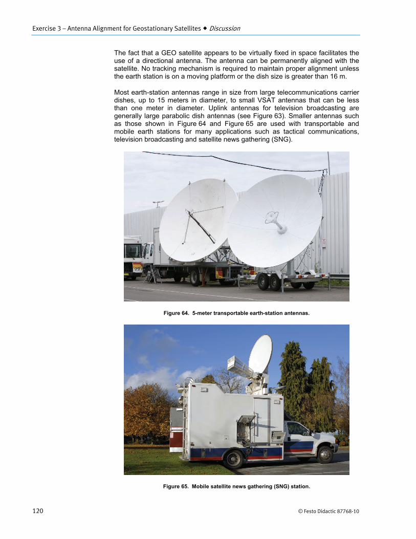
Most earth-station antennas range in size from large telecommunications carrier dishes, up to 15 meters in diameter, to small VSAT antennas that can be less than one meter in diameter. Uplink antennas for television broadcasting are generally large parabolic dish antennas (see Figure 63). Smaller antennas such as those shown in Figure 64 and Figure 65 are used with transportable and mobile earth stations for many applications such as tactical communications, television broadcasting and satellite news gathering (SNG).

Figure 64. 5-meter transportable earth-station antennas.

Figure 65. Mobile satellite news gathering (SNG) station.



Small portable dish antennas, such as that shown in Figure 66 can easily be deployed in the field or on battlegrounds.

Figure 66. Setting up a satellite antenna for a tactical command post (U.S. Marine Corps).



Undoubtedly the most common GEO satellite antenna is the ubiquitous satellite dish, shown in Figure 67, used to receive residential television programming called Direct Broadcast Service (DBS) or Direct-to-Home (DTH) TV.

Figure 67. Satellite DBS dish antennas.

Dish type

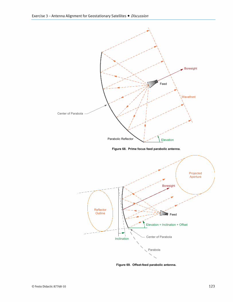
There are several different types of dish antennas. The most common type is the parabolic reflector antenna (see Figure 68). The parabola is illuminated by a source of energy called the feed (usually a waveguide horn) situated at the focus of the parabola and directed towards the center of the parabola.

Because of the characteristics of a parabola, any ray from the feed is reflected by the reflector in a direction parallel to the axis of the parabola. Furthermore, the distance traveled by any ray from the feed to the reflector and then to a plane perpendicular to the axis of the parabola is independent of its path. This means that the signal originating at the feed is converted to a plane wavefront of uniform phase.

The simplest antenna design is the prime focus feed parabolic antenna shown in Figure 68. One disadvantage of this design is that the feed is situated on the boresight and blocks some of the signal. For small dishes, blockage along the boresight causes a significant loss in efficiency. Another disadvantage of this type of antenna, when used for reception, is that the feed horn points downwards toward the ground. Since the feed pattern of the horn is broad and does not stop abruptly at the edge of the dish, spillover from the feed pattern is likely to receive noise from the warm ground. Both of these disadvantages can be remedied by using an offset feed (see Figure 69).



Figure 68. Prime focus feed parabolic antenna.

Figure 69. Offset-feed parabolic antenna.

Parabolic Reflector

Feed

Boresight

Wavefront

Parabola

Feed Reflector Outline

Projected Aperture

Elevation = Inclination + Offset

Boresight

Center of Parabola Inclination

Center of Parabola

Elevation



An offset-feed antenna also has the feed at the focus of the parabola. However, the reflector forms only a section of the parabola. As a result, the feed is no longer on the boresight. If the section does not include the center of the parabola, then none of the radiated beam is blocked by the feed horn. With many antennas, however, the bottom of the reflector coincides with the center of the parabola, as shown in Figure 69. In this case, a small portion of the beam is blocked by the feed, causing a slight loss in efficiency.

Although the antennas shown in Figure 68 and Figure 69 have the same elevation, the feed horn of the offset feed antenna is pointing slightly upwards, which results in less sensitivity to noise from the ground.

The reflector of an offset feed antenna is not perfectly circular, but is slightly elliptical, as shown in Figure 69, with the long axis in the vertical direction. This ensures that the aperture projected along the boresight is circular. The ratio between the short and long axes of the reflector depends on the offset of the antenna:

(34)

When setting the elevation of an offset feed antenna with the satellite, the offset must be taken into account. The elevation of the antenna is equal to the inclination of the reflector plus the offset of the antenna. In Figure 69, it can be seen that the elevation of the antenna is greater than the inclination of the reflector. The difference between the two is the offset.

For example, if the elevation required is 63° and the offset is 22°, the reflector must be inclined at an angle of 41° from the vertical. When the reflector is vertical, the elevation is equal to the offset. If the required elevation is less than the offset, the reflector must be tilted downwards. This may require mounting the reflector upside down or using a special mounting adapter.

Fortunately, in most cases, an elevation scale is built onto the back of the antenna that already compensates for the offset. To adjust the elevation, first ensure that the antenna mast or support is perfectly vertical, and then set the antenna to the desired elevation using the scale.

If the diameter of the main reflector is greater than 100 wavelengths, a Cassegrain antenna is often used (see Figure 70). The Cassegrain antenna is a double reflector type that works on the principle of the Cassegrain optical telescope, invented by the French astronomer Laurent Cassegrain. This design uses a parabolic main reflector and a hyperbolic secondary reflector. The main advantages of this design are reduced size and greater flexibility in the design of the feed system. This design allows for shorter feed lines. Cassegrain antennas are widely used as satellite antennas and as radio telescopes.

When the lower edge of the reflector coincides with the center of the parabola, a line from the lower edge to the feed is approximately parallel to the boresight.



Figure 70. Cassegrain antenna.

With most parabolic dish antennas, the contour of the reflector is round or, in the case of an offset feed antenna, slightly elongated in the vertical direction. However, dish antennas with an elliptical contour are sometimes used in order to achieve high directivity in one plane only while keeping the reflector relatively small. The antenna shown in Figure 71 has higher directivity in the plane of the broad dimension. By aligning the broad axis of the elliptical dish so that it is parallel with the Clarke belt, the directivity of the antenna is optimized.

Feed

Main Reflector

Secondary Reflector



Figure 71. DBS antenna with an elliptical parabolic dish.

Dish size

Table 14 shows earth-station categories based on the size of the parabolic dish antenna.

Table 14. Earth station dish sizes.

Earth Station Category Diameter

Very large dish 15 to 30 m diameter

Large dish 7 to 15 m diameter

Medium dish 3 to 7 m diameter

Small dish 0.5 m to 3 m diameter

The dish size is directly related to the gain of the antenna, which is a measure of how much the antenna focuses the RF signal. The gain varies with direction and is defined as the ratio of the power radiated or received per unit solid angle by the antenna in a given direction to the power radiated or received per unit solid angle by a lossless isotropic antenna fed with the same power.

The gain is maximal along the electromagnetic axis (boresight) of the antenna. When the gain along the boresight is increased, by increasing the diameter of the reflector, the gain in other directions is reduced, making the antenna more directional. When one refers to the “gain” of an antenna, one usually means the maximum gain.

An isotropic antenna is a hypothetical antenna that radiates or accepts power uniformly in all directions



The gain depends on the diameter of the dish, the frequency of the RF signal and an efficiency factor. Figure 72 and Figure 73 show typical relationships between antenna gain and dish size for different frequencies. Figure 72 has a logarithmic horizontal axis and shows that a 1 m dish operating at 4 GHz provides a gain of approximately 30 dB. Doubling the diameter of the dish, or doubling the frequency, increases the gain by 6 dB, that is, by a factor four.

Figure 72. Typical antenna gain versus dish size (0.5 m to 32 m, efficiency factor = 0.6).

Figure 73. Typical antenna gain versus dish size (up to 2 m, efficiency factor = 0.6).

As the dish size, and the gain, increase, the 3 dB beamwidth of the antenna decreases, as shown in Figure 74.

20

30

40

50

60

70

0.5 1 2 4 8 16 32

10

15

20

25

30

35

40

45

50

0 50 100 150 200

For an offset feed antenna, the gain depends on the projected aperture of the antenna.

16 GHz

12 GHz

8 GHz

4 GHz

Dish diameter (m)

Gai

n (d

B)

16 GHz

12 GHz

8 GHz

4 GHz

Dish diameter (cm)

Gai

n (d

B)



Figure 74. 3 dB (half-power) beamwidth versus dish size (efficiency factor = 0.6).

Because of their relatively wide beamwidth, small dish antennas can be permanently aligned with a geostationary satellite and permanently fixed in place. At 12 GHz, a 1-m dish antenna has a beamwidth of approximately 1.8°, which is much greater than the typical station-keeping box limits of ±0.15° for a geostationary satellite. Dishes greater than 16 m, however, have beamwidths less than 0.15° and therefore may require tracking mechanisms to keep them accurately pointed at a geostationary satellite.

Low-noise amplifier (LNA, LNB, LNC, LNBF)

The first active component in a satellite receiver is a special type of amplifier called a low-noise amplifier (LNA) which is used to amplify the weak signal captured by the antenna to a usable level while introducing as little noise as possible. This is followed by a down converter to translate the RF signal to an IF frequency range.

Some receivers use a variation of the LNA called a low-noise converter (LNC), which combines a low-noise amplifier and a down converter. Both the LNA and the LNC have a relatively narrow bandwidth, corresponding to the bandwidth of a single transponder (channel) of the satellite. A type of low-noise converter called the low-noise block (LNB) handles a large bandwidth spanning several or all transponders of the satellite. A low-noise block combined with a down converter is sometimes called a low-noise block converter or low-noise block down converter, although the term low-noise block is often used instead. An LNB combined with a feedhorn is called an LNB feedhorn (LNBF).

Small antennas designed for television reception or data communications usually have an LNBF (often referred to simply as the LNB) at the focus of the antenna. Placing the LNB at the feedhorn instead of in the receiver reduces losses in the coaxial cable between the antenna and the receiver.

Some dish antennas have multiple LNBFs (see Figure 75). This type of antenna is designed to receive signals from two or more different satellites that are closely spaced in longitude. The signal from each satellite must be reflected by the dish to the corresponding LNBF. This requires that each LNBF be adjusted

0.03

0.06

0.13

0.25

0.50

1.00

2.00

4.00

8.00

16.00

0.5 1.0 2.0 4.0 8.0 16.0 32.0

An active component is one that is capable of power gain, such as an amplifier

4 GHz

8 GHz

12 GHz

16 GHz

Dish diameter (m)

3 dB

Bea

mw

idth

(°)



separately. A 22 kHz tone generated by the receiver is applied through the coaxial cable to select the desired satellite.

Figure 75. Dish antenna with multiple LNBFs.

Polarization

An electromagnetic wave is a combination of an electric and a magnetic field. The two fields always appear simultaneously. The plane of the electric field is orthogonal to the plane of the magnetic field and both planes are perpendicular to the direction of propagation. By convention, the polarization of an electromagnetic wave is defined as the orientation of the plane of the electric field.

Polarization can be linear, where the electric field is always oriented at the same angle with respect to a reference plane. For antennas on a satellite, the reference plane is usually the equatorial plane. In most cases, linear-polarization is either horizontal, where the electric field is parallel to the plane of the equator, or vertical. For earth-station antennas, however, the reference plane is the local horizontal plane. Because of the curvature of the earth, these two reference planes are not parallel, unless the earth station and the satellite have the same longitude. The angle between these reference planes is called the polarization angle, or skew. It is the difference between the polarization of the signal transmitted by the satellite and the apparent polarization of the received signal. An adjustment for the polarization angle must be made when aligning a linearly polarized earth-station antenna, in order to maximize the signal.

Polarization can also be elliptical, where the plane of the electric field rotates with time making one complete revolution during one period of the wave. An elliptically polarized wave radiates energy in all planes perpendicular to the direction of propagation. The ratio between the maximum and minimum peaks of the electric field during the rotation is called the axial ratio and is usually specified in decibels. When the axial ratio is near zero dB, the polarization is said to be circular. If the axial ratio is infinite, the electric field maintains a fixed direction and the polarization is linear.

If the rotation is clockwise, looking in the direction of propagation, the polarization is called right-hand. If it is counterclockwise, the polarization is called left-hand.



The polarization of an antenna depends on the shape and the orientation of the waveguide in the feed. The polarization of each antenna in a communications system should be of the same type and, if linear, should be properly aligned. Maximum signal strength at the receiver input occurs when the polarization of the receiving antenna matches the polarization of the incident wave.

Figure 76 shows examples of open waveguides resulting in vertical and horizontal polarization. The waveguide is often energized by a probe protruding through the broad side of the waveguide.

Figure 76. Vertical and horizontal polarization waveguides.

In order to make efficient use of repeater bandwidth, different polarizations are often used for adjacent transponder channels on a satellite. This technique, called polarization diversity, minimizes interference between adjacent channels. It is important therefore, to know the polarization of the satellite transponder you wish to link to in order to correctly configure the earth-station antenna. The polarization may be indicated in reference documents as H (horizontal), V (vertical), RHC, RH or R (right-hand circular) or LHC, LH or L (left-hand circular).

Although linearly polarized antennas can be used to communicate with circularly polarized antennas, there will be an antenna polarization mismatch loss of approximately 3 dB. For a transmitting and receiving antenna both using linear-polarization, the mismatch loss can be up to 20 dB, as shown by Equation (35).

(35)

where is the antenna polarization mismatch loss is the misalignment angle

Circular polarization is often used for satellite communications, particularly for DBS TV broadcasting in North America. With circular polarization, the antenna polarization does not have to be adjusted. This is advantageous because the signal polarization may be rotated as the signal passes through anomalies in the ionosphere. However, it is generally less costly to produce high-performance LNBFs with linear-polarization. When linear-polarization is used, an extra step is required during the alignment procedure in order to correctly adjust the polarization of the antenna.

Many DBS LNBFs are designed for dual polarization (H and V or R and L). A dc voltage of 13 V or 18 V from the receiver is applied to the LNBF through the coaxial cable in order to select the polarization. The lower voltage generally selects the V or R polarization and the higher voltage selects the H or L polarization.

Vertical Polarization

Horizontal Polarization



Some VSAT antennas have a feed assembly with a separate transmit and receive port. This assembly is designed to transmit on one polarization and receive on the other.

Earth station-satellite geometry

Communication with geostationary satellites is almost always done using a directional parabolic antenna. Since it is directional, the antenna must be accurately pointed toward the satellite and then fixed in place.

All geostationary satellites orbit about the earth above the equator, and at the same altitude, in the region of space known as the Clarke belt. Before attempting to align an antenna with a geostationary satellite, it is useful to imagine what the Clarke belt would look like if you could see it in the sky from different locations on earth.

The Clarke belt forms an imaginary arc in the sky (see Figure 77). If you are at the equator, the belt passes directly overhead. If you are in the northern hemisphere, the belt stretches from a point on the horizon a little south of due east, rising to its maximum height directly towards the south, and then reaching the horizon a few degrees south of due west. If you are in the southern hemisphere, the maximum height of the arc appears directly north of your location.

Figure 77. The Clarke belt and antenna look angles (in the northern hemisphere).

Geographic NorthTrue Azimuth

Elevation

Maximum Elevation = 90° - Latitude – Elevation Declination

Local Horizontal

Clarke Belt



The true azimuths of all geostationary satellites that are visible from a location in the northern hemisphere range from a little more than 90° to a little less than 270°. For locations in the southern hemisphere, the true azimuths are greater than 270° or less than 90°.

The elevation of geostationary satellite can range from a little more than 0° (local horizontal) to a maximum elevation that depends on the latitude of the earth station. For an earth station at the equator, the maximum possible elevation is 90°. For latitudes north or south of the equator, the maximum possible elevation is equal to 90° minus the latitude minus the apparent declination .

a Absolute values of the latitude and the apparent declination are used here because the signs of these values are different in the northern and southern hemispheres.

Look angles for geostationary satellites are usually calculated assuming a spherical, rather than an ellipsoidal, earth. This introduces an error in antenna orientation between 0.02° and 0.03°. This error, however, has little effect on the performance of small dish antennas because their beamwidth is considerably greater than the error. In this exercise, a spherical earth is assumed and no distinction is made between geocentric and geodetic latitude.

The apparent declination , shown in Figure 78, arises from the fact that the geostationary satellites are not at an infinite distance, as is the celestial equator, but are located approximately 36 000 km from the surface of the earth. This apparent declination varies with the latitude of the earth station and is not the same as the true declination of a GEO satellite which is always close to zero. Since declination is always measured with respect to the celestial equator, the apparent declination of a geostationary satellite is negative for an observer in the northern hemisphere (at positive latitudes) and positive for an observer in the southern hemisphere (at negative latitudes).

Figure 78. Geostationary satellite maximum elevation (satellite and earth station at the same longitude).

The apparent declination for a GEO satellite at the same longitude as the earth station can be calculated as shown in Equation (36). Its magnitude ranges from 0 at the equator to approximately 8.7 at a latitude of ±80 , which is near the extreme limit for linking with a GEO satellite. For satellites not at the same longitude as the earth station, the apparent declination is slightly different, but varies by less than one degree over the visible region of the Clarke belt.

When the elevation to a satellite is high, the path of the signal through the at-mosphere is relatively short and degradation due to the atmosphere is low. When the elevation is low, the signal follows a much longer path through the atmos-phere and degradation is higher. The effect is signifi-cant below 10° elevation and very severe below 5°.

Local Zenith

To Celestial Equator

Equator

Local Horizontal

EarthStation

Earth-station latitude Radius of the earth

Geocentric radius of the satellite Geostationary altitude

Apparent declination Maximum elevation



(36)

where is the apparent declination of the GEO satellite is the earth’s radius (6378 km) is the geostationary satellite radius (42 164 km) is the latitude of the earth station

Since the position of a geostationary satellite is fixed with respect to the earth, and because we are assuming a spherical earth, all calculations of azimuth and elevation can be performed in a terrestrial (EFG) coordinate system using the earth station latitude and longitude as well as the satellite longitude and radius.

The longitude sat of a geostationary satellite is the longitude of the subsatellite point on the earth's surface. The radius of the satellite (distance from the center of the earth) is equal to the satellite’s altitude plus the radius of the earth.

The location of the earth station on the surface of earth can also be specified in the EFG coordinate system frame using the earth station’s longitude es and latitude .

Because azimuth and elevation are measured relative to the position of the earth station on the earth’s surface, and not to the center of the earth, a topocentric horizontal coordinate system must be used. This is a spherical coordinate system whose origin is centered on the earth station. Since both the position of the satellite and the position of the earth station, expressed in the EFG system are known, equations can be used to express the position of the satellite in the azimuth-elevation coordinate system. Figure 79 and Figure 80 show the geometry involved. (Figure 80 is a screen shot from the Orbit Simulator with added texts and arrows.)



Figure 79. Azimuth-elevation geometry for a geostationary satellite.

XEF

G

Z EFG

E

arth

-sta

tion

latit

ude

E

arth

-sta

tion

long

itude

f

Sat

ellit

e lo

ngitu

de

A

zim

uth

E

leva

tion

R

adiu

s of

the

earth

Geo

cent

ric ra

dius

of t

he s

atel

lite

G

eost

atio

nary

alti

tude

Sla

nt ra

nge

Equ

ator

N

Equ

ator

ial P

lane

C

lark

e B

elt

Loca

l Zen

ith

Loca

l Hor

izon

tal P

lane

Gre

enw

ich

Mer

idia

n



Figure 80. Earth-satellite geometry with EFG axes.

The azimuth can be calculated as shown in Equation (37).

In the northern hemisphere ( ):

In the southern hemisphere ( ):

(37)

where is the azimuth in degrees is the earth station latitude in degrees is the difference in longitude, in degrees, between the earth station

and the satellite

a Because , the sign of is important in Equation (37). is positive when the earth station is east of the satellite.

By convention, longitudes to the east are positive and longitudes to the west are negative, unless given in degrees west. For an earth station at a longitude of 80 W and a satellite at 90 W, .

The angular distance between the earth station and the subsatellite point is given by:

(38)

There are many software tools and Web sites availa-ble that facilitate these calculations. If you enter these equations into a spread sheet, be sure to convert all angles to radians and then convert the result into degrees.

Greenwich Meridian

Earth StationMeridian

SatelliteMeridian

Antenna Azimuth

Antenna Elevation

GEO Satellite

Equator

Earth Station

North Pole

Earth Station Parallel

Subsatellite Point

AntennaBoresight

Earth station latitude Earth station longitude Satellite longitude

Longitude difference Angular distance

LVSAT Orbit Simulator



Equations (39) shows how the elevation can be calculated.

(39)

where is the elevation in degrees is angular distance between the earth station and the subsatellite

point is the radius of the earth is the radius of the satellite is the earth station latitude in degrees is the difference in longitude, in degrees, between the earth station

and the satellite

For a geostationary satellite, the ratio is

(40)

To predict the performance of the satellite communications system, it is important to know the slant range . This can be calculated using Equation (41).

(41)

where is the slant range (the distance from the earth station to the satellite)

Figure 81 shows a graph of the elevation to the Clarke belt versus azimuth for an earth station located at a latitude of 45 (blue curve). The dots on the blue curve represent geostationary satellites spaced 10 apart around the Clarke belt. Because the earth station is in the northern hemisphere, the GEO satellite with the highest elevation is at an azimuth of 180 , that is, due south. Satellites whose longitudes are east or west of that of the earth station have lower elevations.



Figure 81. Geostationary satellite elevation vs. azimuth at latitude 45 .

The blue line in Figure 81 was calculated using Equation (37) and Equations (39), using the ratio . This ratio applies to all satellites on the Clarke belt. The red line represents the celestial equator, which is the imaginary circle in the plane of the equator located at an infinite distance from the earth.

As expected, the maximum elevation to the celestial equator is equal to 90 minus the latitude of the earth station. The red dots represent the projections of the GEO satellites onto the celestial equator. The difference in degrees between a satellite and its projection on the celestial equator is the apparent declination which was illustrated in Figure 78.

Figure 82. Geostationary satellite elevation vs. azimuth at latitude 70 .

Figure 82 shows a similar graph for an earth station at a latitude of 70 and illustrates the problem with linking to geostationary satellites at latitudes far from the equator. The maximum elevation angle is very low and a smaller part of the Clarke belt is visible at an elevation of 10° or more.

The polarization of the signal is also important. The most common polarizations are linear and circular. To ensure adequate reception of the signal, both the transmitting antenna and the receiving antenna must be designed to use the same type polarization.

If circular polarization is used, no special adjustment of the earth-station antenna is required. The feed horn or LNBF of the antenna, however, must use circular polarization of the same direction (right-hand or left-hand).

0

10

20

30

40

50

90100110120130140150160170180190200210220230240250260270

0

10

20

30

90100110120130140150160170180190200210220230240250260270

Celestial Equator

Ele

vatio

n (

)

Azimuth ( )

Clarke Belt

Celestial EquatorE

leva

tion

()

Azimuth ( )

Clarke Belt

Apparent Declination

Apparent Declination



If linear-polarization is used, however, the curved surface of the earth causes the local horizontal plane to be tilted, or skewed, with respect to the polarization of the satellite antenna when the earth station and the satellite are at different longitudes (see Figure 83). As a result, the feed horn or LNBF of the earth-station antenna must be rotated by the same angle in order to prevent attenuation.

Figure 83. Depolarization due to the earth's curvature.

Equation (42) shows how the skew (polarization angle) can be calculated.

(42)

where is the skew (polarization angle) of the earth-station antenna is the earth station latitude in degrees is the difference in longitude, in degrees, between the earth station

and the satellite

Skew



Antenna look angle and skew adjustments

Figure 84 shows a typical offset-feed parabolic antenna mounted on a tripod. The dish is supported by a vertical mast. A feed arm attached to the dish supports the low-noise block feedhorn (LNBF).

Figure 84. Offset-feed parabolic dish antenna on tripod.

Figure 85 shows the adjustments for azimuth, elevation and skew. Antennas designed for use with GEO satellites usually move about two orthogonal axes. The primary axis is fixed with respect to the earth and is usually adjusted to be perfectly vertical so that movement about this axis sets the azimuth. The secondary axis is horizontal and rotates about the primary axis. Movement about this axis sets the elevation.

Mast (Pole)

Tripod

LNBF

Feed Arm

Dish

Base

Adjustable Feet



Skew is adjusted by rotating the LNBF. Facing towards the satellite, a positive rotation is clockwise and a negative rotation is counter-clockwise.

Figure 85. Antenna look-angle adjustments.

Figure 86 shows a close-up of the elevation scale.

Figure 86. Elevation scale.

Azimuth Axis

Elevation Axis

Azimuth Locking Nuts

Elevation Locking Nut

Positive Rotation

Skew Adjustment:

Elevation Scale

Elevation Locking Nut

Elevation Scale (°)

Negative Rotation



With many antennas, either a linear or a circular polarization LNBF can be installed. Figure 87 shows an example of the two types.

Figure 87. Typical circular and linear polarization LNBFs.

When a linear-polarization LNBF is used, the skew must be adjusted by rotating the LNBF. A scale is usually provided to aid in making this adjustment, as shown in Figure 88.

Figure 88. Skew adjustment for linear-polarization.

Circular Polarization Linear Polarization

Negative Rotation Positive Rotation

Skew Scale (°)

LNBF Clamp



Aligning a small dish antenna with a geostationary satellite

Equipment required for alignment

To mount and align an antenna, the following equipment is required:

a Consult the manufacturer’s documentation provided with the antenna, the LNBF and all other equipment to be used.

The antenna, the LNBF, an antenna mount and all necessary hardware.

The tools required to tighten the nuts or screws that set the azimuth, elevation and skew.

A signal strength indicator which can be one of the following:

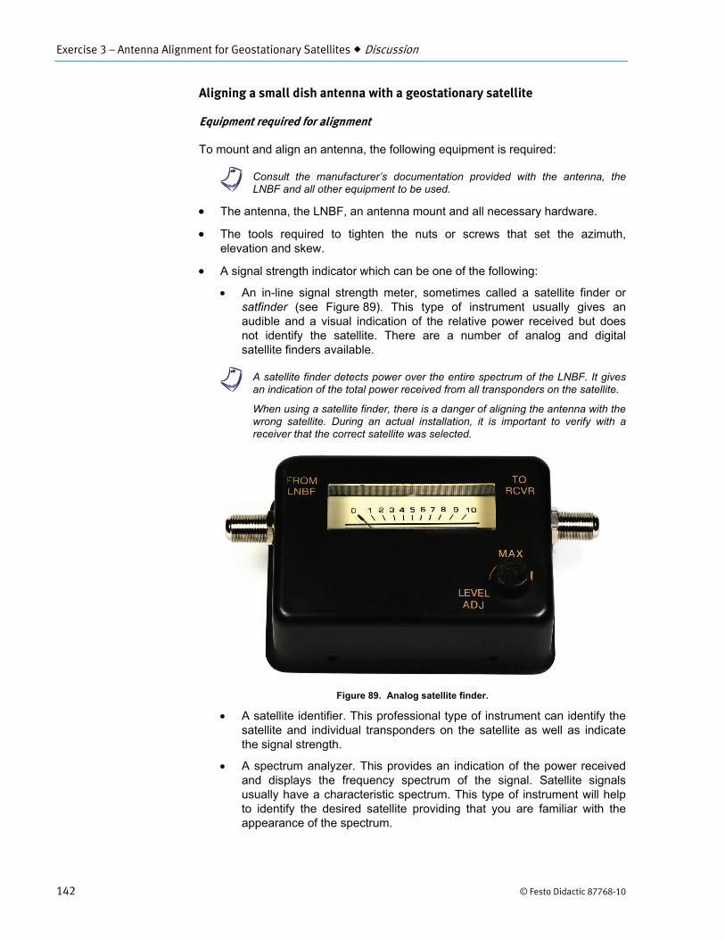
An in-line signal strength meter, sometimes called a satellite finder or satfinder (see Figure 89). This type of instrument usually gives an audible and a visual indication of the relative power received but does not identify the satellite. There are a number of analog and digital satellite finders available.

a A satellite finder detects power over the entire spectrum of the LNBF. It gives an indication of the total power received from all transponders on the satellite.

When using a satellite finder, there is a danger of aligning the antenna with the wrong satellite. During an actual installation, it is important to verify with a receiver that the correct satellite was selected.

Figure 89. Analog satellite finder.

A satellite identifier. This professional type of instrument can identify the satellite and individual transponders on the satellite as well as indicate the signal strength.

A spectrum analyzer. This provides an indication of the power received and displays the frequency spectrum of the signal. Satellite signals usually have a characteristic spectrum. This type of instrument will help to identify the desired satellite providing that you are familiar with the appearance of the spectrum.



A commercial satellite receiver and TV. This will indicate when the desired signal is being received and also provide an indication of the signal strength and quality. However, it can be inconvenient to use outdoors and may require time to lock onto the signal. It may be very difficult to determine the optimal antenna position using this method.

A level to adjust the mount so the mast will be perfectly vertical, ensuring that the scale on the antenna bracket will be fairly accurate and that the azimuth and elevation adjustments will be independent. If there is no elevation scale on the antenna, or if the mast is not vertical, an inclinometer can be used to indicate the antenna elevation directly.

An inclinometer or clinometer is an instrument for measuring angles of elevation, inclination or tilt of an object with respect to gravity. Commercial inclinometers are available for aligning satellite antennas, or a homemade one can be made using a protractor and a short plumb line.

a The built-in elevation scale may not be very accurate. However, it should be accurate enough to allow you to find the satellite, after which you can optimize the elevation in order to maximize the received signal power.

A magnetic compass or GPS receiver to determine azimuth.

Additional equipment, such as a dc source (battery pack) or a 22 kHz tone generator may be required to actuate switching circuits built into the LNBF (consult the documentation provided with the LNBF). These are usually incorporated into a satellite receiver and are built into some satellite finders. If this is not the case, the dc source or tone generator must be connected to the Receiver connector of the satellite finder.

Some spectrum analyzers can be damaged if a dc voltage is applied to the input. If the cable from the antenna has a dc voltage, a dc block (dc blocking capacitor) may be required at the input of the spectrum analyzer.

General alignment procedure

The following procedure summarizes the steps required to align a small dish antenna to a geostationary satellite.

a When aligning a dish antenna with multiple LNBFs, first align the antenna using the central LNBF and tighten all settings. When this is completed, adjust the position and skew (if using linear polarization) of each of the other LNBFs to maximize the signals from the corresponding satellites.



1. Obtain the following information about the satellite and the transponder you wish to link to (there are various websites and software tools available for this purpose):

The longitude of the satellite.

The frequency band of the satellite.

The type of polarization used by the satellite (linear or circular) and the polarization used by the transponder whose signals you wish to receive.

The footprint of the transponder beam you wish to receive, if possible. Make sure that the earth station is located within this footprint.

The minimum recommended dish size for your location. This depends on the power of the satellite transponders and on the elevation and slant range to the satellite.

2. Make sure you have an LNBF that is appropriate for the frequency band and polarization used and that the dish meets or exceeds the recommended minimum size.

3. Determine the geographic coordinates (latitude and longitude) of the earth station. This can be done using a GPS receiver, a mapping website, or a software tool designed for this purpose.

4. If you will be setting the azimuth using a magnetic compass, determine the magnetic declination for your location. b The easiest way to determine the magnetic declination for your location is to

use one of the many websites that provide this information (see Appendix E Useful Websites). If this is not possible, refer to Appendix B Magnetic Declination. This appendix shows how to compensate for magnetic declination and includes a world map of magnetic declination contours that will allow you to determine the approximate magnetic declination for your location.

5. Determine the required antenna elevation, azimuth and skew. The necessary equations are provided in the Discussion. There are also several websites and software tools available for this purpose.

a In this exercise, the satellite longitude and polarization as well as the antenna elevation, azimuth and skew can be supplied by the Orbit Simulator.

These angles only need to be determined to a precision of approximately one degree. The scales on most antennas are not very precise and allow only an approximate adjustment that will help you to find the satellite. Once the satellite is found, you will “tweak” the look-angle adjustments to maximize the signal strength.

Skew adjustment of the LNBF is only required if the satellite uses linear-polarization (see Step 9). However, if the dish is elliptical, it is always preferable to adjust the skew of the dish (see Step 18).

6. Conduct a site survey at the antenna location to determine if the antenna will be able to “see” the satellite once the elevation and azimuth are set. If obstacles will block the signal, choose a different location.

7. If necessary, assemble the antenna mount or tripod according to the manufacturer’s instructions. It may also be necessary to assemble the feed arm and install the LNBF.

The magnetic declination at any point on the earth is the angle between the local magnetic field—the direc-tion the north end of a com-pass points to—and true north. The declination is positive when the magnetic north is east of true north and negative when it is west of true north.



8. Install the mast on a stable surface or on a tripod. Use a level to make sure that the mast is perfectly vertical.

9. If the satellite beam uses linear polarization, set the skew of the LNBF. In a permanent installation, it is usually easier to do this before you mount the antenna on the mast.

a If the dish is elliptical and the feed arm is fixed onto the dish, setting the skew of the dish sets the skew of the LNBF. It may be easier to do this at the end of the procedure.

a As shown in Appendix C Satellite Transponders, the downlink beam of a satellite is composed of signals from many transponders using different polarizations. Because a satellite finder detects power over the entire transponder bandwidth, it cannot distinguish between individual frequencies as a receiver does. For this reason, changing the skew of the LNBF is not likely to change the signal strength displayed by the satellite finder. Setting the skew correctly will, however, improve the strength of the signal detected by the receiver.

To set the skew, orient the feed horn or LNBF the same as the nominal polarization of the transponder beam. For vertical polarization, the broad faces of the waveguide are on the top and bottom, as shown in Figure 76. If you have a dual-polarization LNBF, the default polarization is usually vertical.

Then rotate the LNBF the same number of degrees as the skew angle determined in Step 5. Looking from behind the dish towards the LNBF and the satellite, a positive rotation is clockwise and a negative rotation is counter-clockwise.

10. If not already done, install the antenna on the mast according to the manufacturer’s instructions.

11. Set the elevation as determined in Step 5 using the scale on the antenna or an inclinometer. Tighten the elevation adjustment bolts until they are snug.

a It is usually easier to set and lock the elevation first, as this prevents the antenna from tilting down under its own weight, and then set the azimuth.

12. Set the azimuth as determined in Step 5. If you are using a compass, make sure to compensate for magnetic declination. Tighten the azimuth locking nuts just enough to avoid accidental movement of the antenna.

a Be sure to hold the compass where it will not be affected by metal objects.

It may be helpful to identify a building or other object located in the desired direction, and then point the antenna in that direction.



13. Connect the signal strength indicator to the LNBF using a coaxial cable according to the manufacturer’s instructions. If a dc source or 22 kHz tone generator is required, connect it to the Receiver connector on the detector.

If the LNBF is designed for dual polarization selected using a dc voltage, make sure that the low voltage is being applied.

If the antenna uses a 22 kHz tone to select different satellites, set this tone as required.

14. Observing the signal strength indicator, slowly vary the azimuth of the antenna until you find the satellite. Depending on the satellite and the location of the earth station, it may require some time to find the desired satellite.

a If the indicator saturates on a strong signal, activate the built-in attenuator.

15. Fine tune the azimuth by moving the antenna slightly from one side to the other. Identify two points on either side where the signal strength decreases by the same amount, then position the antenna in the center. Tighten the azimuth locking nuts until they are snug and verify that the antenna has not moved.

16. Check the elevation and azimuth adjustments by bending the dish slightly in both the vertical and horizontal directions (push or pull gently on the edge of the dish). When you bend the dish, the signal level as shown on the detector should decrease slightly. When you remove pressure from the dish, it should spring back to its original position and the signal level should increase.

17. Firmly tighten the elevation and azimuth locking nuts and check the adjustments again.

18. If the dish is elliptical, tilt the long axis of the dish to the skew angle determined in Step 5. The long axis of the dish, shown as a dashed line in Figure 90, should be approximately parallel to the Clarke belt. If the feed arm is fixed to the dish, this will also set the skew of the LNBF.

The dc voltage sets the polarization of the LNBF as follows:

13 V: V or R 18 V: H or L

Since the LNBF may draw a considerable amount of current, use a battery-powered indicator sparingly. Activating the high voltage may drain the battery more quickly.

Exercise 3 – Antenna Alignment for Geostationary Satellites Procedure Outline


Figure 90. Elliptical dish alignment.

The Procedure is divided into the following sections:

GEO maximum elevation Visibility of the Clarke belt Antenna look angles Preparation for pointing the antenna Pointing a dish antenna

Pointing a dish antenna

The last section of the Procedure requires a dish antenna and accessories. In this section, you will set up the antenna outdoors and align it with several different geostationary satellites. You will require the following items:

Parabolic dish antenna Linear-polarization LNBF Circular-polarization LNBF Satellite finder Coaxial cable

Tripod Magnetic level Wrench Screwdriver Compass Tape measure

PROCEDURE OUTLINE

Clarke Belt

Axis of Greatest Directivity

Exercise 3 – Antenna Alignment for Geostationary Satellites Procedure


GEO maximum elevation

In this section, you will determine the maximum elevation to a geostationary stationary satellite from several different locations on earth.

1. Start the LVSAT Orbit Simulator software.

Load the file GEO.xml (remove all current satellites).

Show the Earth Station Location as a Meridian-Parallel.

Show the Azimuth/Elevation Angles and the Earth-Satellite Geometry.

Make sure Time is paused at 00:00:00.

For each city in Table 15, use the Orbit Simulator to determine the maximum elevation angle of a GEO satellite for that location.

Then calculate the maximum elevation angle using the equations in the Discussion and compare these with the observed maximum elevation angles. b Modify the orbital elements of the satellite as required to facilitate your

observations. Recall that the elevation is highest when the satellite and the earth station have the same longitude.

You may wish to change the 3D Earth setting as you wish in order to show the earth’s surface or reveal all of the earth-satellite geometry.

Table 15. Cities and maximum elevation to a GEO satellite.

City Latitude Longitude Observed maximum elevation

Calculated maximum elevation

Sydney, Australia

Abidjan, Côte d’Ivoire

Tokyo, Japan

Boston, MA

Berlin, Germany

Moscow, Russia

North Pole

Explain why Santa Claus cannot receive satellite TV programs broadcast from a GEO satellite.

The elevation to a GEO satellite is at its maximum when the satellite is at the same longitude as the earth station. In the Orbit Simulator, at Time 00:00:00,

. Therefore, the longitude of a GEO satellite is equal to:

PROCEDURE



Therefore, to observe the maximum elevation in the Orbit Simulator, set one of these orbital elements equal to the longitude of the earth station and leave the others set to zero. The Information window will indicate that the longitude of the satellite and that of the earth station are equal. The Elevation displayed in the Information window will then be the observed maximum elevation for the satellite at the current earth station location.

Table 15. Cities and maximum elevation to a GEO satellite.

City Latitude Longitude Observed maximum elevation

Calculated maximum elevation

Sydney, Australia -33.51 151.12 51.03 51.03

Abidjan, Côte d’Ivoire 5.20 -4.01 83.88 83.88

Tokyo, Japan 35.42 139.42 48.87 48.87

Boston, MA 42.36 -71.06 41.09 41.09

Berlin, Germany 52.30 13.24 30.19 30.19

Moscow, Russia 55.45 37.37 26.79 26.79

North Pole 90.00 0.00 -8.6 -8.6

The maximum elevation can be calculated using:

where is the earth station latitude. The declination is:

The maximum elevation from the North Pole to a GEO satellite is negative. This means that all GEO satellites are below the local horizon and are therefore not visible from that location.

Visibility of the Clarke belt

In this section, you will observe how the latitude of the earth station affects the visibility of the Clarke belt.

2. Set the Earth Station City to Mexico City, Mexico. Use the Orbit Simulator to determine what percentage of the Clarke belt is visible from this location with an elevation of 10° or more. Then do the same for Edmonton, Alberta and compare your results for the two cities using Table 16. b You can set the satellite longitude so that the elevation from the earth station is

approximately 10° as shown in Figure 91. Then you can fine tune the satellite longitude while observing the Elevation displayed in the Information window.



Figure 91. Determining the satellite longitude for 10° elevation to Mexico City.

Table 16. Percentage of Clarke belt visible at 10° elevation or more.

Value Symbol Mexico City Edmonton

Earth station latitude

Earth station longitude

Satellite longitude for 10° elevation

Longitude difference

Percentage of Clarke belt visible at 10° elevation or more

10° Elevation Contour

Mexico City

Earth Station Parallel

Earth Station Meridian

Azimuth

Elevation

Longitude Difference

LVSAT Orbit Simulator

Subsatellite Point



How does the latitude of the earth station affect the visibility of the Clarke belt?

Table 16. Percentage of Clarke belt visible at 10° elevation or more.

Value Symbol Mexico City Edmonton

Earth station latitude 19.26° 53.57°

Earth station longitude -99.08° -113.52°

Satellite longitude for 10° elevation -28.79° or -169.37

-55.95° or -171.1

Longitude difference 70.29° 57.57°

Percentage of Clarke belt visible at 10° elevation or more 39% 32%

The closer the Earth station is to the equator, the greater the visible portion of the Clarke belt.

Antenna look angles

In this section, you will calculate the azimuth, elevation and skew angles for geostationary satellites and compare your results to the angles shown in the Orbit Simulator.

3. Load the file Geostationary (active).txt (remove all current satellites).

a This file shows most of the active geostationary satellites using the orbital elements that were available at the time of writing.

A text satellite file contains a Two-Line Element (TLE) set for each satellite which gives the actual parameters for the satellite as they were measured at a given epoch. Because geostationary satellites drift and require periodic corrections, the orbital positions defined by these parameters may be slightly different from the assigned orbital positions.

Hide the Paths of all satellites.

Show the Azimuth/Elevation Angles and the Earth-Satellite Geometry.

If you live in one of the cities listed in the Orbit Simulator, set the Earth Station City to your city. If not, set the Earth Station Latitude and Longitude to the geographical coordinates of your location. b Many websites allow you to determine your geographical coordinates precisely

(see Appendix E Useful Websites). A GPS receiver can also be used, if you have one. Alternately, an atlas will provide your approximate coordinates.

Click on a satellite whose longitude is close to the longitude of the Earth station, in order to activate it. The azimuth and elevation angles are shown graphically in the 3D view. The Information window displays the Azimuth, Elevation and Skew as numerical values. Activate satellites further and further from your longitude as you observe these angles.



b When the Earth-Satellite Geometry is shown, a line is drawn from the Earth Station to the active satellite as long as the elevation is positive. No line is shown when the elevation negative.

You may wish to try this while viewing the Earth from above the North or South Pole.

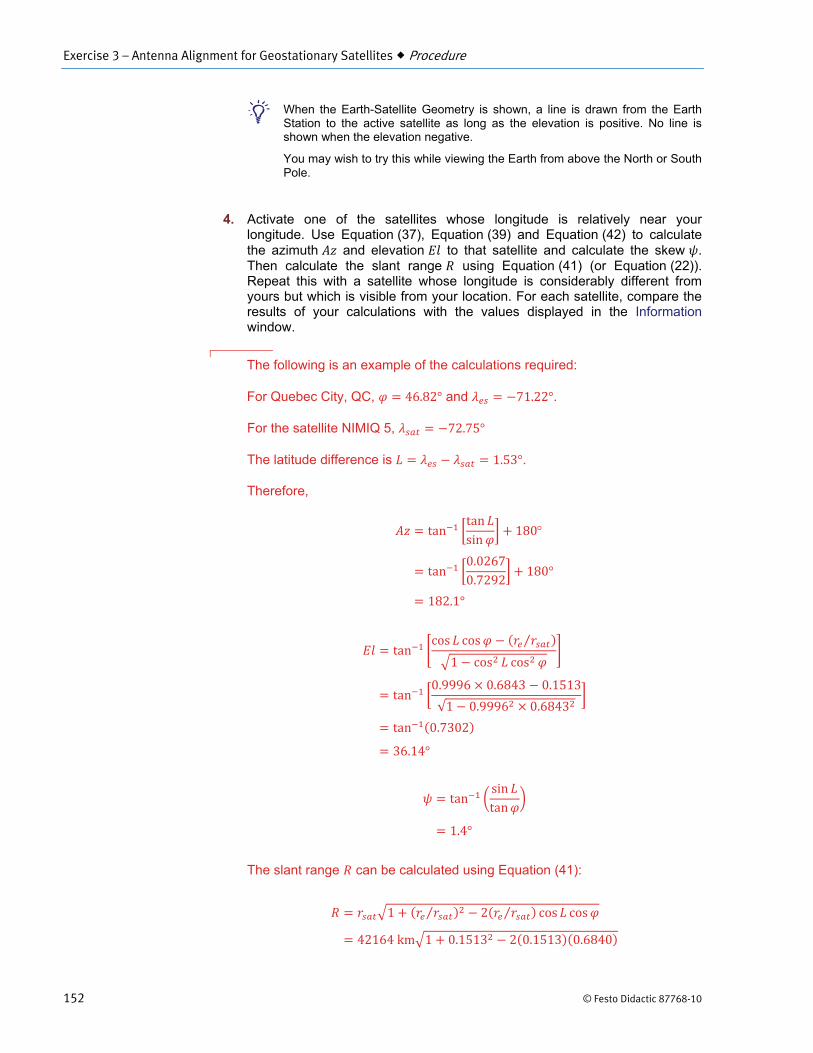
4. Activate one of the satellites whose longitude is relatively near your longitude. Use Equation (37), Equation (39) and Equation (42) to calculate the azimuth and elevation to that satellite and calculate the skew . Then calculate the slant range using Equation (41) (or Equation (22)). Repeat this with a satellite whose longitude is considerably different from yours but which is visible from your location. For each satellite, compare the results of your calculations with the values displayed in the Information window.

The following is an example of the calculations required:

For Quebec City, QC, and .

For the satellite NIMIQ 5,

The latitude difference is .

Therefore,

The slant range can be calculated using Equation (41):



Alternately, the slant range can be calculated from the elevation using Equation (22).

In the Information window, Azimuth = 182.1°, Elevation = 36.16°, Skew = 1.44°, Slant Range = 38078.4 km.

Preparation for pointing the antenna

In this section, you will gather the information necessary to align a dish antenna with real geostationary satellites. To do this, you will use the Orbit Simulator to select several geostationary satellites that are visible from your location and that transmit in the Ku band (approximately 12 to 18 GHz). You will determine the type of polarization used by each satellite and determine the look angles as well as the magnetic azimuth.

5. Load the file Geostationary Ku-band (EW).xml (remove all current satellites).

Hide the Path of each satellite. Show the Earth-Satellite Geometry.

This file contains most of the geostationary satellites that transmit in the Ku band (approximately 12 to 18 GHz). The satellites are shown in their assigned positions and not at their actual positions observed at a certain epoch.

The name of each satellite is preceded by its assigned longitude in degrees East or West, as shown in Table 17.

Table 17. Examples of satellite names in Geostationary Ku-band (EW).xml.

Displayed Name Satellite Name Longitude

E003 Telecom 2C Telecom 2C 3° E

E013 Hotbird 9 Hotbird 9 13° E

E122 Asiasat 4 Asiasat 4 122° E

W000.8 Thor 5 Thor 5 0.8° W (-0.8° E)

W129 Ciel 2 Ciel 2 129° W (-129° E)

a A similar file, called Geostationary Ku-band (E).xml, is also included with the Orbital Simulator. In this file, the displayed names begin with the longitude in degrees East, ranging from 0° to 360°.



6. Make sure that the Latitude and Longitude settings in the Orbit Simulator correspond to your location. Record your location, latitude and longitude below.

Location (city, town, village, etc.):

Latitude (°N):

Longitude (°E):

Magnetic declination:

Determine the magnetic declination for your location and record it, using a positive value for eastward declination and a negative value for westward declination. b Many websites allow you to determine your geographical coordinates precisely

(see Appendix E Useful Websites). Many GPS receivers can display the magnetic declination after the position is established. Alternately, a world map in Appendix B Magnetic Declination can be used to determine your approximate magnetic declination.

Each GEO satellite used for television broadcasting has one or more transponders and each transponder on the satellite transmits at a different frequency and at a particular polarization: horizontal (H), vertical (V), right-hand circular (R), or left-hand circular (L). Most satellites with several transponders transmit using two different polarizations: linear (H and V) or circular (R and L).

The currently loaded satellite file (Geostationary Ku-band (EW).xml) uses different colors to show the polarizations used by each satellite, as shown in Table 18.

Using the Orbit Simulator, determine which portion of the Clarke belt is visible from your location. Select at least five satellites that will be visible. Referring to the color code used in Table 18, try to select satellites that broadcast using as many different polarizations as possible. Enter the names of these satellites in the appropriate rows, entering more than one satellite per row if necessary. Later in this exercise, you will set up a dish antenna outdoors and align it with these satellites.

a The Orbit Simulator does not show the footprints of the satellites. In some cases, the name of the satellite indicates the service zone it is intended to cover (e.g. Eurobird, Asiasat, Chinasat). It is possible that the beam from a visible satellite does not cover your location. For this reason, it is preferable to select a few extra satellites.



Table 18. Ku-band satellites for pointing the antenna.

Polarization and color Satellite Names Longitude

(°E) True

Azimuth (°) Magnetic

Azimuth (°) Elevation

(°) Skew

(°)

H only (Red)

H and V (Yellow)

V only (Green)

R and L (Blue) (not

required)

Both linear and circular

(Grey)

a Some satellites are colored grey even if they transmit only one type of polarization because they are so close to a satellite that uses the other type of polarization that it would be difficult to separate the two signals.

Activate in turn each satellite entered in Table 18 and record the Azimuth (true azimuth), the Elevation, and the Skew displayed in the Information window. Then determine the magnetic azimuth for each satellite and enter this in the table as well. b Enter the longitudes West with a minus sign, as shown in the Information

window.

You can round off the numbers you enter in this table. The scales on most antennas allow setting look angles to approximate values only.

If you prefer, you can use one of the dish pointing web sites or software tools to obtain the look angles for these satellites (see Appendix E Useful Websites). Make sure the satellites transmit in the Ku band.



The following is an example of a valid answer for the indicated location.

Location (city, town, village, etc.): Quebec City, QC

Latitude (°N): 46.82

Longitude (°E): -71.22

Magnetic declination: -16.6° (16° 37 W)

Table 18. Ku-band satellites for pointing the antenna.

Polarization and color Satellite Names Longitude

(°E) True

Azimuth (°) Magnetic

Azimuth (°) Elevation

(°) Skew

(°)

H only (Red) Star One C1 -65.0 171.5 188.1 35.8 -5.6

H and V (Yellow) Galaxy 16 -99.0 215.9 232.3 29.7 23.5

V only (Green) Intelsat 1R -50.0 152.0 168.6 32.3 -18.8

R and L (Blue) Anik F3 -118.7 236.1 252.7 19.4 (not

required)

Both linear and circular

(Grey) Galaxy 17 -91 206.1 222.7 32.7 17.5

The magnetic azimuth for the first satellite in Table 18 is calculated as follows:



Pointing a dish antenna

This section requires a dish antenna and accessories. Please refer to the procedure outline for a complete list of the required items. In this section, you will set up a dish antenna outdoors and align it with several geostationary satellites.

a It is preferable to work in teams of two students while carrying out the steps in this section.

7. Read the instructions provided with the satellite finder and become familiar with its operation.

8. The dish antenna should be assembled and mounted on its tripod.

Examine the dish antenna. Describe the type of antenna.

This is a small offset parabolic dish antenna.

This response is given as an example and depends on your antenna.

Measure the height and width of the dish. What is the diameter of the projected aperture?

The dimensions of one model are approximately 82 cm by 75 cm. The projected aperture is approximately 75 cm.


Referring to Figure 73, estimate the gain of the antenna when operating at 12 GHz.

The gain of the antenna is approximately 37 dB at 12 GHz.


Determine the approximate offset of the antenna.

The approximate offset is given by:


9. Set up the dish antenna on its tripod outdoors at a location where the selected satellites should be visible.

Exercise 3 – Antenna Alignment for Geostationary Satellites Conclusion


Follow the alignment procedure given in the Discussion in order to point the antenna to each of the selected satellites. For each satellite, you must make sure that the correct LNBF (linear or circular polarization) is installed on the antenna.

If any of the satellites you have selected uses only one polarization (H, V, R or L), then you may be able to observe polarization mismatch loss. With the satellite pointed at the antenna, change the polarization of the LNBF and note whether the signal level increases or decreases.

a If a satellite transmits with both horizontal and vertical polarization, changing the polarization of the LNBF will make little or no difference in the signal strength indicated by the satellite finder. This is because a satellite finder does not discriminate between different frequencies. When performing a real antenna installation, however, it is important to adjust the skew of the LNBF because the receiver is tuned to only one frequency at a time.

10. When you have finished using the dish antenna and its accessories, bring all items inside and return them to their proper location.

If you have not already done so, exit the Orbital Simulator software when you have finished using it.

In this exercise, you learned about antenna alignment for geostationary satellites. You became familiar with the different type of parabolic dish antennas and LNBFs used with geostationary satellites. You became familiar with the theory behind antenna alignment to geostationary satellites and with look angle and polarization skew adjustments. If you have a parabolic dish antenna, you aligned this antenna with several different geostationary satellites.

1. All geostationary satellites are located on the Clarke belt. Describe what the Clarke belt would look like if you could see it from the earth.

The Clarke belt forms an imaginary arc in the sky. If you are at the equator, the belt passes directly overhead. If you are in the northern hemisphere, the belt stretches from a point on the horizon a little south of due east, rising to its maximum height directly towards the south, and then reaching the horizon a few degrees south of due west. If you are in the southern hemisphere, the maximum height of the arc appears directly north of your location. The elevation to the center of the Clarke belt is equal to 90° minus the latitude minus the apparent declination .

CONCLUSION

REVIEW QUESTIONS

Exercise 3 – Antenna Alignment for Geostationary Satellites Review Questions


2. What is the purpose of the low-noise amplifier in a receiving earth station? Describe the different types of low noise amplifier used in satellite reception.

The low-noise amplifier (LNA) is used to amplify the weak signal captured by the antenna to a usable level while introducing as little noise as possible. A low-noise converter (LNC) combines a low-noise amplifier and a down converter. A low-noise block (LNB) handles a large bandwidth spanning several or all transponders of the satellite and often includes a down converter. A low-noise block feedhorn (LNBF) is a low-noise block combined with a feedhorn.

3. Explain why dish antennas are often used in satellite earth stations.

A parabolic dish antenna is used for high gain and directivity. Directivity is a measure of the degree to which the radiated energy is concentrated in one direction and is proportional to the square of the dish diameter. High directivity in transmission allows the power to be directed towards the desired satellite while minimizing interference to other satellites. High directivity in reception allows minimizing the interference received from other satellites and nearby earth stations.

4. Explain why alignment of an earth-station antenna to a geostationary satellite can be done using a coordinate system fixed to the earth.

To an observer on the earth, a geostationary satellite appears to be fixed in space because its orbital period is synchronized with the earth’s rotation and because its inclination is near 0 . Therefore, the position of the satellite, as well as the position of the earth station, can be conveniently expressed using any coordinate system attached to the terrestrial reference frame.

5. When aligning a small dish antenna with a geostationary satellite that uses linear polarization, what is the order in which you should normally adjust the three angles. Explain why.

The skew of the LNB is normally adjusted first for two reasons: because it is usually easier to adjust this before mounting the antenna on the mast, and because it is not possible to tweak the skew using a satellite finder when the satellite uses both horizontal and vertical polarization. The elevation is adjusted next and the elevation locking bolt tightened to prevent the elevation changing accidently. Finally, with the antenna free to pivot on the principal axis, the azimuth can be set in order to find the satellite and maximize the received power.


Bibliography

Satellite Communications for the Nonspecialist

Satellite Communications Systems

Fundamentals of Astrodynamics

Fundamentals of Astrodynamics and Applications

Rocket and Space Technology, 2008.

Orbital and Celestial Mechanics Website

CelesTrak

satellite orbits, coverage, and antenna alignment

Documents