savings and economic impacts of the better buildings ... · final report savings and economic...
TRANSCRIPT
Prepared For:
U.S. Department of Energy Office of Energy Efficiency and Renewable Energy
Prepared For:
U.S. Department of Energy Office of Energy Efficiency and Renewable Energy
Final Report
Savings and Economic Impacts of the Better Buildings Neighborhood Program
Final Evaluation Volume 2
American Recovery and Reinvestment Act of 2009
June 2015
DOE/EE-1203

DOE/EE-1203
Final Report
Savings and Economic Impacts of the Better Buildings Neighborhood Program
Final Evaluation Volume 2
American Recovery and Reinvestment
Act of 2009
June 2015
Funded By:
Prepared By:
Research Into Action, Inc.
Evergreen Economics
Nexant, Inc.
NMR Group, Inc.
Prepared For:
U.S. Department of Energy
Office of Energy Efficiency and Renewable Energy

www.researchintoaction.com
PO Box 12312
Portland, OR 97212
3934 NE Martin Luther King Jr. Blvd., Suite 300
Portland, OR 97212
Phone: 503.287.9136
Fax: 503.281.7375
Contact:
Jane S. Peters, President

Savings and Economic Impacts of the Better Buildings Neighborhood Program DOE/EE-1203
Final Evaluation Volume 2
Acknowledgements | Page i
ACKNOWLEDGEMENTS
This research project was initiated and directed by Jeff Dowd of the U.S. Department of Energy’s (DOE)
Office of Energy Efficiency & Renewable Energy (EERE). Project management and technical oversight
was provided by Edward Vine, Staff Scientist, of Lawrence Berkeley National Laboratory (LBNL), and Yaw
Agyeman, Project Manager at LBNL.
Our team of evaluators would like to thank Jeff and Ed for their support and guidance on this project.
We also would like to thank the staff of DOE’s Better Buildings Neighborhood Program (BBNP). Danielle
Sass Byrnett led the staff, with key program support provided by Steve Dunn and Dale Hoffmeyer, as
well as by account managers and numerous contractors. We thank Danielle and her staff and
contractors for their openness and willingness to talk with us at length and answer numerous email
questions.
We interviewed all 41 BBNP grant recipients, as well as 6 subgrantees, and requested project
documentation and other information from many of these contacts. The grantees and subgrantees had
many people wanting them to explain their activities and their accomplishments during the past five
years; although we were one of the many, they were overwhelmingly friendly and cooperative, usually
talking with us for several hours to explain what they were doing and what their experiences had been.
We anticipate future discussions will continue to illuminate the varied activities and accomplishments of
BBNP, and we look forward to those discussions.
We are grateful to the technical advisors that Ed Vine assembled for this research. They guided our
detailed evaluation plans and reviewed our draft reports. Their critiques, insights, and interpretations
greatly improved the work. Our peer review team comprised Marian Brown, Phil Degens, Lauren Gage,
and Ken Keating. Lisa Petraglia and John A. (“Skip”) Laitner reviewed the economic impact analysis. Our
DOE review team comprised Jeff Dowd and Dale Hoffmeyer. Preliminary research also was reviewed by
DOE staff Danielle Sass Byrnett, Claudia Tighe, and Bill Miller.
Finally, DOE staff, their contractors, and LBNL and National Renewable Energy Laboratory (NREL) staff
related to BBNP were all extremely responsive to our team’s requests for data and were very helpful
during the planning and implementation of the evaluation activities. They understood program realities
and continually worked to improve the program and its offerings. In addition, they were continually
balancing the need for accuracy in reporting without trying to overburden the grantees that are
oftentimes short-staffed and over-worked.

Savings and Economic Impacts of the Better Buildings Neighborhood Program DOE/EE-1203
Final Evaluation Volume 2
Notice | Page ii
NOTICE
This document was prepared as an account of work sponsored by an agency of the United States
government. Neither the United States government nor any agency thereof, nor any of their employees,
makes any warranty, express or implied, or assumes any legal liability or responsibility for the accuracy,
completeness, usefulness, or any information, apparatus, product, or process disclosed, or represents
that its use would not infringe privately owned rights. Reference herein to any specific commercial
product, process, or service by trade name, trademark, manufacturer, or otherwise does not necessarily
constitute or imply its endorsement, re commendation, or favoring by the United States government or
any agency thereof. The views and opinions of authors expressed herein do not necessarily state or
reflect those of the United States government or any agency thereof.

Savings and Economic Impacts of the Better Buildings Neighborhood Program DOE/EE-1203
Final Evaluation Volume 2
Table of Contents | Page I
TABLE OF CONTENTS
Glossary .............................................................................................................. XV
Preface ............................................................................................................... XIX
Executive Summary ........................................................................................ ES-1
Evaluation Objectives and Methods ................................................................................ ES-1
BBNP Goals and Objectives ............................................................................................ ES-2
Goal and Objective Attainment ........................................................................................ ES-3
Energy, Environmental, and Economic Impacts .............................................................. ES-8
Impact Assessment Lessons Learned ........................................................................... ES-10
Recommendations ........................................................................................................ ES-11
1. Introduction ........................................................................................................1
1.1. Study Overview .............................................................................................................. 1
1.2. BBNP Description .......................................................................................................... 2
1.3. BBNP Goals and Objectives .......................................................................................... 4
1.4. Program Terminology ..................................................................................................... 5
2. Better Buildings Neighborhood Program ...........................................................6
2.1. Reported Program Accomplishments ............................................................................. 6
2.1.1. Reported Through Q3 2013 (The Evaluation Period) ........................................................... 6
2.1.2. Reported Through Q3 2014 (The End of the Extension Period) ........................................ 10
2.2. Grantee Programs ....................................................................................................... 11
2.3. Program Requirements ................................................................................................ 13
2.4. Databases and Data Tracking Processes .................................................................... 14
2.4.1. Grantee Data Reporting and Tracking................................................................................ 14
2.4.2. DOE Reporting Processes ................................................................................................. 15
3. Methodology ................................................................................................... 17
3.1. Overview ...................................................................................................................... 17
3.2. M&V ............................................................................................................................. 18
Savings and Economic Impacts of the Better Buildings Neighborhood Program DOE/EE-1203
Final Evaluation Volume 2
Table of Contents | Page II
3.3. Billing Regression Analysis .......................................................................................... 18
3.4. Extrapolation of Results to Overall BBNP ..................................................................... 18
3.5. Overall Verified BBNP Savings .................................................................................... 19
3.6. Additional Overall BBNP Metrics .................................................................................. 20
3.6.1. Greenhouse Gas Emission Savings ................................................................................... 20
3.6.2. Lifetime Energy Savings ..................................................................................................... 21
3.6.3. Estimating Annual and Lifetime Bill Savings ...................................................................... 21
3.6.4. Leveraged Funds ................................................................................................................ 22
3.7. Net-to-Gross Methods .................................................................................................. 22
3.7.1. Lower Bound Net-to-Gross Ratio Estimates Derived from Participating End Users .......... 23
3.7.2. Upper Bound Net-to-Gross Ratio Estimates Derived from Participating and
Nonparticipating Contractors .............................................................................................. 24
3.8. Economic Impact Analysis ........................................................................................... 25
3.9. Review of Independent Evaluations ............................................................................. 26
3.10. Assessing Grantee Success ....................................................................................... 27
3.11. Sampling .................................................................................................................... 29
3.12. Limitations and Challenges......................................................................................... 31
3.12.1. Self-Reported Tracking Data ............................................................................................ 31
3.12.2. Difficulty Interpreting Grantee Data .................................................................................. 32
3.12.3. Inaccuracies of DOE Reported Metrics ............................................................................ 32
3.12.4. Delayed or Lack of Grantee Responsiveness .................................................................. 33
3.12.5. Limited Value of Participant Phone Verification Surveys ................................................. 33
3.12.6. Large Scope and Broad Scale of Grantee Programs ...................................................... 34
3.12.7. Limited Billing Data Available ........................................................................................... 34
3.12.8. Lack of Incremental Measure Cost .................................................................................. 34
4. Findings .......................................................................................................... 35
4.1. Energy Impact Estimates ............................................................................................. 35
4.2. Environmental Impact Estimates .................................................................................. 38
4.3. Economic Impact Estimates ......................................................................................... 39
4.4. Leveraged Funds Estimates ......................................................................................... 40

Savings and Economic Impacts of the Better Buildings Neighborhood Program DOE/EE-1203
Final Evaluation Volume 2
Table of Contents | Page III
4.5. M&V Additional Findings .............................................................................................. 40
4.5.1. M&V Sample Extrapolation ................................................................................................. 42
4.5.2. Factors Contributing to Realization Rate Estimate ............................................................. 42
4.6. Billing Regression Analysis Findings ............................................................................ 43
4.6.1. Final Model Specification Results ....................................................................................... 43
4.6.2. Billing Regression Analysis Realization Rates ................................................................... 46
4.7. Estimating BBNP Energy and Other Savings ............................................................... 47
4.7.1. Combining the M&V and Billing Regression Analysis Findings ......................................... 47
4.7.2. Extrapolating to the BBNP Population ................................................................................ 48
4.7.3. Confidence and Precision ................................................................................................... 48
4.7.4. Net-to-Gross Analysis Findings .......................................................................................... 49
4.8. Environmental Impact Analysis Additional Findings ..................................................... 49
4.9. Economic Impact Analysis Additional Findings............................................................. 50
4.9.1. Gross Economic Impacts .................................................................................................... 51
4.9.2. Net Economic Impacts ........................................................................................................ 54
4.9.3. Net Economic Impact of Energy Bill Savings in Post Installation Years ............................ 57
4.9.4. Benefit-Cost Ratio ............................................................................................................... 61
4.10. Leveraged Resources ................................................................................................ 61
4.10.1. Financial Institution Funds ................................................................................................ 61
4.10.2. Other Leveraged Funds ................................................................................................... 63
4.10.3. Summary .......................................................................................................................... 65
5. Lessons Learned, Conclusions, and Recommendations ............................... 66
5.1. Lessons Learned ......................................................................................................... 66
5.1.1. Grantee Interaction ............................................................................................................. 66
5.1.2. Sampling ............................................................................................................................. 66
5.1.3. Evaluation Activities ............................................................................................................ 67
5.1.4. Reporting Infrastructure ...................................................................................................... 67
5.2. Conclusions ................................................................................................................. 68
5.2.1. Goal and Objective Attainment ........................................................................................... 68
5.2.2. Impact Assessment Lessons Learned................................................................................ 72
Savings and Economic Impacts of the Better Buildings Neighborhood Program DOE/EE-1203
Final Evaluation Volume 2
Table of Contents | Page IV
5.3. Recommendations ....................................................................................................... 72
References .......................................................................................................... 74
Appendices .......................................................................................................... 76
Appendix A. Grantee Awards ...................................................................... A-1
Appendix B. Impact Evaluation Methodology Supplement ......................... B-1
B.1. Overview .................................................................................................................... B-1
B.1.1. Components of the Research ............................................................................................B-1
B.1.2. Timing of Evaluation Activities ...........................................................................................B-2
B.1.3. Relationship to Preliminary Evaluation Methodology ........................................................B-4
B.2. Sampling Methods ..................................................................................................... B-4
B.2.1. Overview of M&V and Regression Sampling Approaches ................................................B-4
B.2.2. Overlap of M&V and Regression Samples ........................................................................B-4
B.2.3. M&V Sample ......................................................................................................................B-4
B.3. Measurement and Verification Methods ................................................................... B-15
B.3.1. Obtaining Grantee Project Records .................................................................................B-15
B.3.2. Designing the Data Collection Instruments .....................................................................B-16
B.3.3. Conducting Onsite Verifications ......................................................................................B-17
B.3.4. Conducting Project File Reviews .....................................................................................B-17
B.3.5. Establishing the Baseline Scenarios ...............................................................................B-17
B.3.6. Verifying Gross Impacts ..................................................................................................B-18
B.4. Billing Regression Methods ...................................................................................... B-20
B.4.1. Model Specifications ........................................................................................................B-21
B.4.2. Data Cleaning ..................................................................................................................B-22
B.5. Review of Independent Evaluations ......................................................................... B-24
B.6. Net-to-Gross Methodology ....................................................................................... B-26
B.6.1. Lower Bound Net-to-Gross Ratio Estimates derived from participating end users .........B-26
B.6.2. Upper Bound Net-to-Gross Ratio Estimates derived from participating and
nonparticipating contractors ............................................................................................B-29
B.7. Extrapolation of Results to Overall BBNP ................................................................. B-35
Savings and Economic Impacts of the Better Buildings Neighborhood Program DOE/EE-1203
Final Evaluation Volume 2
Table of Contents | Page V
B.7.1. M&V Extrapolation ...........................................................................................................B-35
B.7.2. Billing regression analysis Extrapolation .........................................................................B-36
B.7.3. Overall BBNP Extrapolation ............................................................................................B-36
B.8. Additional Overall BBNP Metrics .............................................................................. B-45
B.8.1. Greenhouse Gas Emission Savings ................................................................................B-45
B.8.2. Lifetime Energy Savings ..................................................................................................B-45
B.9. Economic Impact Analysis Methods ......................................................................... B-47
B.9.1. Analysis Methods .............................................................................................................B-47
B.9.2. Model Input Data .............................................................................................................B-52
B.10. Leveraging (James Wolf Methodology and Application) ......................................... B-58
Appendix C. Billing Regression Findings Supplement ................................ C-1
C.1. Final Model Results ................................................................................................... C-1
C.2. Models by residential subsector: Single-family, Multifamily Units, and Multifamily
Buildings .................................................................................................................... C-6
C.2.1. Natural Gas Models .......................................................................................................... C-9
C.3. Confidence and Precision ........................................................................................ C-12
Appendix D. Alternate Billing Regression Model Specifications.................. D-1
D.1. Logged Consumption ................................................................................................. D-1
D.2. Interacted Weather .................................................................................................... D-5
D.3. Commercial Models with Added Control..................................................................... D-9
D.3.1. Consumer Price Index .................................................................................................... D-10
D.3.2. Personal Income ............................................................................................................. D-12
D.3.3. Proprietor Income ........................................................................................................... D-15
D.4. Measure-Specific Models ......................................................................................... D-17
D.4.1. Number of Different Types of Measures Installed .......................................................... D-18
D.4.2. Categories of Measures Installed ................................................................................... D-22
D.4.3. Retrofit Comprehensiveness .......................................................................................... D-28
D.5. Model with Matched Controls ................................................................................... D-34
D.5.1. Matched Comparison Group Models .............................................................................. D-34
D.5.2. Adjusted Final Model Specification ................................................................................. D-34
Savings and Economic Impacts of the Better Buildings Neighborhood Program DOE/EE-1203
Final Evaluation Volume 2
Table of Contents | Page VI
D.5.3. Monthly Consumption Model Specification .................................................................... D-37
D.6. Weighted Annual Consumption ................................................................................ D-42
D.7. Normalized Annual Consumption ............................................................................. D-47
Appendix E. Alternative Billing Data Screens ............................................. E-1
Appendix F. Fuel Prices .............................................................................. F-1
Appendix G. Weather Data ......................................................................... G-1
Appendix H. Common Measure Savings Sources and Equations .............. H-1
H.1. List of Sources ........................................................................................................... H-1
H.2. Lighting-Residential ................................................................................................... H-1
H.3. Lighting-Commercial .................................................................................................. H-2
H.4. Furnace/Boiler Replacement – Residential ................................................................ H-2
H.5. AC, Central – Residential and Small Commercial ...................................................... H-2
H.6. Air Sealing ................................................................................................................. H-3
H.7. Insulation ................................................................................................................... H-4
Appendix I. Fuel Conversions ..................................................................... I-1
Appendix J. Residential and Commercial Verification Surveys .................. J-1
J.1. Residential Participant: Better Buildings Neighborhood Programs Telephone
Survey ........................................................................................................................ J-1
J.1.1. General Information (From Grantee Documentation) ........................................................ J-1
J.1.2. Project Measure Information (From Grantee Documentation) .......................................... J-1
Appendix K. Residential and Commercial Pre-Notification Letters ............. K-1
K.1. Residential Letter ....................................................................................................... K-1
K.2. Commercial Letter ...................................................................................................... K-2
Appendix L. Grantee Leveraging Questions Interview Guide ..................... L-1
L.1. Interview Details ..........................................................................................................L-1
L.2. Response Matrix .........................................................................................................L-1
L.3. Intro ............................................................................................................................L-1
Savings and Economic Impacts of the Better Buildings Neighborhood Program DOE/EE-1203
Final Evaluation Volume 2
Table of Contents | Page VII
L.4. Sources.......................................................................................................................L-2
L.5. Activities......................................................................................................................L-2
L.6. Timing of Program’s Contribution ................................................................................L-3
L.7. Character of Program’s Contribution ...........................................................................L-3
L.8. Resources Contributed by Program ............................................................................L-3
L.9. Close ..........................................................................................................................L-4
LIST OF TABLES
Table ES-1: ARRA Goals ........................................................................................................................ ES-3
Table ES-2: BBNP Objectives................................................................................................................. ES-3
Table ES-3: Attainment of ARRA Goals, through Q3 2013 .................................................................... ES-5
Table ES-4: Attainment of BBNP Objectives .......................................................................................... ES-6
Table ES-5: Verified Gross and Net Energy Savings, through Q3 2013 ................................................ ES-8
Table ES-6: Annual and Lifetime Bill Savings Associated with Verified Net Energy Savings, through Q3 2013 .......................................................................................................................................... ES-8
Table ES-7: Verified Annual and Lifetime Avoided Carbon Emissions (CO2e), through Q3 2013 ......... ES-9
Table ES-8: Estimated Gross and Net Economic Activity and Tax Revenues, through Q3 2013 .......... ES-9
Table ES-9: Estimated Gross and Net Benefit-Cost Ration and Jobs Impact, through Q3 2013 ......... ES-10
Table 1-1: Key Metrics .................................................................................................................................. 2
Table 1-2: ARRA Goals ................................................................................................................................. 4
Table 1-3: BBNP Objectives ......................................................................................................................... 5
Table 2-1: BBNP Reported (Unverified) Progress Q4 2010 - Q3 2013 ........................................................ 6
Table 2-2: BBNP Reported (Unverified) Projects and Energy Savings Q4 2010 - Q3 2013 ........................ 7
Table 2-3: Average BBNP Reported (Unverified) Savings per Project by Sector ........................................ 7
Table 2-4: BBNP Reported (Unverified) Site Energy Savings through Q3 2013 by Fuel Type per Sector ................................................................................................................................................... 8
Table 2-5: Summary of BBNP Reported Upgrade and Loan Accomplishments through Q3 2014 ............ 10
Table 2-6: Count of BBNP Reported Residential Upgrades by Calendar Year .......................................... 10
Table 2-7: Summary of BBNP Reported (Unverified) Energy Savings through Q3 2014........................... 10
Table 2-8: Technologies and Services Offered by Grantees Across the Four Sectors .............................. 12
Table 3-1: Summary of Methods ................................................................................................................. 18
Table 3-2: Billing Regression Adjustment Factors ...................................................................................... 19
Table 3-3: Energy Cost Prices .................................................................................................................... 21
Table 3-4: Net-to-Gross Ratio Calculation Methods ................................................................................... 24
Savings and Economic Impacts of the Better Buildings Neighborhood Program DOE/EE-1203
Final Evaluation Volume 2
Table of Contents | Page VIII
Table 3-5: Grantee Sample Frame by Evaluation Activity .......................................................................... 29
Table 3-6: Preliminary Evaluation Proposed and Achieved M&V Sample Size by Sector ......................... 30
Table 3-7: Final Evaluation Proposed and Achieved M&V Sample Size by Sector ................................... 31
Table 4-1: Reported and Gross Verified Source Savings, through Q3 2013 .............................................. 35
Table 4-2: Average Site Energy Savings as Proportion of Baseline Energy Use....................................... 36
Table 4-3: Annual Bill Savings Associated with Reported and Verified Energy Savings ........................... 36
Table 4-4: Net Verified Source Savings, through Q3 2013 ......................................................................... 37
Table 4-5: Net Lifetime Source Energy Savings, through Q3 2013 ............................................................ 37
Table 4-6: Reported and Verified Site Energy Savings by Fuel Type and Sector, through Q3 2013......... 38
Table 4-7: Net Verified Annual and Lifetime Avoided CO2e, through Q3 2013 .......................................... 38
Table 4-8: Estimated Gross and Net Economic Activity and Tax Revenues, through Q3 2013 ................. 39
Table 4-9: Estimated Gross and Net Benefit-Cost Ratio and Jobs Impact, through Q3 2013 ................... 39
Table 4-10: Leveraged Funds, through Q3 2013 ........................................................................................ 40
Table 4-11: M&V Realization Rate by Sector for Q1 2010 – Q2 2012 ....................................................... 40
Table 4-12: M&V Realization Rate by Sector for Q3 2012 - Q3 2013 ........................................................ 40
Table 4-13: Combined Preliminary and Final M&V Realization Rates for Verified Source Savings .......... 41
Table 4-14: Residential Combined M&V Realization Rates by Fuel Type ................................................. 41
Table 4-15: Commercial Combined M&V Realization Rates by Fuel Type ................................................ 41
Table 4-16: Multifamily Combined M&V Realization Rates by Fuel Type .................................................. 42
Table 4-17: Electricity Billing Regression Model Output ............................................................................. 43
Table 4-18: Natural Gas Billing Regression Model Output ......................................................................... 44
Table 4-19: Electricity and Natural Gas Billing Regression Model Summary ............................................. 45
Table 4-20: Billing Regression Analysis Realization Rate by Sector for Q1 2010 – Q3 2013 .................... 46
Table 4-21: Billing Regression Analysis Residential Realization Rate by Fuel Type ................................. 46
Table 4-22: Billing Regression Analysis Commercial Realization Rate by Fuel Type ................................ 46
Table 4-23: Billing Regression Analysis Multifamily Realization Rate by Fuel Type .................................. 47
Table 4-24: Residential Combined Realization Rate .................................................................................. 47
Table 4-25: Commercial Combined Realization Rate ................................................................................. 48
Table 4-26: Multifamily Combined Realization Rate ................................................................................... 48
Table 4-27: Reported and Gross Verified Source Savings, Q1 2010 – Q3 2013 ....................................... 48
Table 4-28: Confidence, Precision, and Error Bound by Sector for Gross Verified Savings ...................... 48
Table 4-29: Sector Net-To-Gross Estimates ............................................................................................... 49
Table 4-30: Residential Sector Net Verified and Lifetime Avoided CO2e through Q3 2013 ....................... 50
Table 4-31: Commercial Sector Net Verified and Lifetime Avoided CO2e through Q3 2013...................... 50
Table 4-32: Agricultural Sector Net Verified and Lifetime Avoided CO2e through Q3 2013 ....................... 50
Table 4-33: Summary of BBNP Spending and Energy Savings Used for Economic Impact Modeling ...... 51
Savings and Economic Impacts of the Better Buildings Neighborhood Program DOE/EE-1203
Final Evaluation Volume 2
Table of Contents | Page IX
Table 4-34: BBNP Gross Direct Economic Impacts, by Quarter ................................................................ 52
Table 4-35: BBNP Gross Direct Economic Impacts, by Type, through Q3 2013 ....................................... 53
Table 4-36: BBNP Total Economic Impacts, Gross and Net, through Q3 2013 ......................................... 55
Table 4-37: BBNP Net Direct Economic Impacts, Federal Non-Defense Spending Counterfactual, by Type, through Q3 2013 .................................................................................................................. 55
Table 4-38: BBNP Net Economic Impacts, Taxpayer Rebate Counterfactual, by Type, through Q3 2013 .................................................................................................................................................... 56
Table 4-39: BBNP Gross Impact Measure Sensitivity to 10% Increase in Inputs/Outlays ......................... 57
Table 4-40: BBNP Net Impact Measure Sensitivity to 10% Increase in Inputs/Outlays ............................. 57
Table 4-41: Net Economic Impacts Due to Annualized Energy Bill Savings Alone .................................... 59
Table 4-42: BBNP Total Economic Impacts, Program and Future Year .................................................... 60
Table 4-43: Benefit-Cost Ratio, through Q3 2013 ...................................................................................... 61
Table 4-44: Types of Financing Support Grantees Provided ...................................................................... 62
Table 4-45: Reported Leveraged Funds (Federal and Non-federal) .......................................................... 63
Table 4-46: Non-Federal Leveraged Funds Reported and Those Meeting Wolf’s More Conservative Definition ............................................................................................................................................. 64
Table 4-47: Sources of Leveraged Funds Meeting Wolf’s Definition .......................................................... 64
Table 4-48: Leveraged Funds, through Q3 2013 ........................................................................................ 65
Table 5-1: Attainment of ARRA Goals, through Q3 2013 ........................................................................... 69
Table 5-2: Attainment of BBNP Objectives ................................................................................................. 70
Table A-1: BBNP Grant Recipients ............................................................................................................A-1
Table A-2: BBNP Recipient Grant Recipients in Decreasing Order of Grant Amounts .............................A-2
Table B-1: Summary of Major Final Impact Evaluation Project Deliverables ............................................B-2
Table B-2: Schedule of Major Evaluation Activities ...................................................................................B-3
Table B-3: Actual M&V Sampling by Sector for Preliminary Evaluation ....................................................B-7
Table B-4: Actual M&V Sampling by Sector for Final Evaluation ..............................................................B-7
Table B-5: Residential M&V Sample Design by Substrata (Q3 2012 – Q3 2013) .....................................B-8
Table B-6: Final Residential M&V Sample ...............................................................................................B-10
Table B-7: Commercial Sample Design by Strata (Q3 2012 - Q3 2013) .................................................B-11
Table B-8: Final Commercial M&V Sample .............................................................................................B-13
Table B-9: Multifamily M&V Sample Design by Substrata (Q3 2012 - Q3 2013) ....................................B-14
Table B-10: Final Multifamily M&V (MVMF) Sample ...............................................................................B-15
Table B-11: Baseline Measure Data Used for Analysis ...........................................................................B-18
Table B-12: Reference Documents Used M&V Analysis .........................................................................B-19
Table B-13: Summary of Electricity and Natural Gas Billing Regression Data Screens .........................B-24
Table B-14: Benchmarking Results: Participation and Sample Size .......................................................B-24
Table B-15: Benchmarking Results: Gross Savings and Savings per Project ........................................B-25
Savings and Economic Impacts of the Better Buildings Neighborhood Program DOE/EE-1203
Final Evaluation Volume 2
Table of Contents | Page X
Table B-16: Benchmarking Results: Methods Used to Determine Energy Savings ................................B-25
Table B-17: Net-to-Gross Ratio Calculation Methods ..............................................................................B-26
Table B-18: Free-ridership Influence Scoring ..........................................................................................B-28
Table B-19: Complete List of Free-ridership Net-to-Gross Data Sources ...............................................B-29
Table B-20: Adjusted Residential Spillover Estimate Used in Upper Bound NTG Estimate ...................B-30
Table B-21: Examples of Estimating Contractors’ Net BBNP Upgrades .................................................B-33
Table B-22: Single-family Electric Adjustment Factor Regression Model Results ..................................B-38
Table B-23: Commercial Electric Adjustment Factor Regression Model Results ....................................B-39
Table B-24: Distribution of the Adjustment Factor Sample ......................................................................B-39
Table B-25: BBNP Outlays by Major Outlay Category ............................................................................B-52
Table B-26: Summary of BBNP Efficiency Upgrades, by Sector .............................................................B-55
Table B-27: Reported Annual Energy Savings, by Fuel Type, and Estimated Annual Bill Savings ........B-57
Table C-1: Descriptive Statistics – Residential Electricity Model .............................................................. C-1
Table C-2: Detailed Residential Electricity Model Results ........................................................................ C-1
Table C-3: Descriptive Statistics – Residential Natural Gas Model .......................................................... C-2
Table C-4: Detailed Residential Natural Gas Model Results .................................................................... C-2
Table C-5: Descriptive Statistics – Commercial Electricity Model ............................................................ C-3
Table C-6: Detailed Commercial Electricity Model Results ...................................................................... C-3
Table C-7: Descriptive Statistics – Commercial Natural Gas Model......................................................... C-4
Table C-8: Detailed Commercial Natural Gas Model Results ................................................................... C-4
Table C-9: Residential Electricity and Natural Gas Fuel Savings by Grantee .......................................... C-5
Table C-10: Commercial Electricity and Natural Gas Fuel Savings by Grantee ...................................... C-5
Table C-11: Residential Electricity Savings by Building Type .................................................................. C-6
Table C-12: Descriptive Statistics – Single-family Electricity Model ......................................................... C-6
Table C-13: Single-family Electricity Model Results ................................................................................. C-6
Table C-14: Descriptive Statistics – Multifamily Units Electricity Model ................................................... C-7
Table C-15: Multifamily Units Electricity Model Results ............................................................................ C-7
Table C-16: Descriptive Statistics – Multifamily Building Electricity Model ............................................... C-8
Table C-17: Multifamily Buildings Electricity Model Regression Results .................................................. C-8
Table C-18: Residential Natural Gas Savings by Building Type............................................................... C-9
Table C-19: Descriptive Statistics – Single-family Natural Gas Model ..................................................... C-9
Table C-20: Single-family Natural Gas Model Results ............................................................................. C-9
Table C-21: Descriptive Statistics – Multifamily Units Natural Gas Model ............................................. C-10
Table C-22: Multifamily Units Natural Gas Model Results ...................................................................... C-10
Table C-23: Descriptive Statistics – Multifamily Building Natural Gas Model ......................................... C-11
Table C-24: Multifamily Buildings Natural Gas Model Results ............................................................... C-11
Savings and Economic Impacts of the Better Buildings Neighborhood Program DOE/EE-1203
Final Evaluation Volume 2
Table of Contents | Page XI
Table D-1: Descriptive Statistics – Residential Logged Electric Model .................................................... D-2
Table D-2: Logged Electricity Model Regression Results - Residential ................................................... D-2
Table D-3: Descriptive Statistics – Commercial Logged Electric Model ................................................... D-2
Table D-4: Logged Electricity Model Regression Results – Commercial ................................................. D-3
Table D-5: Descriptive Statistics –Residential Logged Natural Gas Model .............................................. D-3
Table D-6: Logged Natural Gas Model Regression Results – Residential ............................................... D-4
Table D-7: Descriptive Statistics – Commercial Logged Natural Gas Model ........................................... D-4
Table D-8: Logged Natural Gas Model Regression Results – Commercial ............................................. D-4
Table D-9: Descriptive Statistics – Residential Interacted Weather Electric Model .................................. D-6
Table D-10: Interacted Weather Electric Model Regression Results – Residential.................................. D-6
Table D-11: Descriptive Statistics – Commercial Interacted Weather Electric Model .............................. D-7
Table D-12: Interacted Weather Electric Model Regression Results – Commercial ................................ D-7
Table D-13: Descriptive Statistics – Residential Interacted Weather Natural Gas Model ........................ D-8
Table D-14: Interacted Weather Natural Gas Model Regression Results – Residential .......................... D-8
Table D-15: Descriptive Statistics – Commercial Interacted Weather Natural Gas Model ....................... D-9
Table D-16: Interacted Weather Natural Gas Model Regression Results – Commercial ......................... D-9
Table D-17: Descriptive Statistics – Commercial Consumer Price Index Electric Model ....................... D-10
Table D-18: Consumer Price Index Electric Model Regression Results – Commercial ......................... D-11
Table D-19: Descriptive Statistics – Commercial Consumer Price Index Natural Gas Model ................ D-11
Table D-20: Consumer Price Index Natural Gas Model Regression Results – Nonresidential .............. D-12
Table D-21: Descriptive Statistics – Nonresidential Personal Income Electric Model ............................ D-13
Table D-22: Personal Income Electric Model Regression Results – Nonresidential .............................. D-13
Table D-23: Descriptive Statistics – Nonresidential Personal Income Natural Gas Model .................... D-14
Table D-24: Personal Income Natural Gas Model Regression Results – Nonresidential ...................... D-14
Table D-25: Descriptive Statistics – Nonresidential Proprietor Income Electric Model .......................... D-16
Table D-26: Proprietor Income Electric Model Regression Results – Nonresidential ............................ D-16
Table D-27: Descriptive Statistics – Nonresidential Proprietor Income Natural Gas Model ................... D-17
Table D-28: Proprietor Income Natural Gas Model Regression Results – Nonresidential ..................... D-17
Table D-29: Descriptive Statistics – Residential Measure Count Electric Model .................................... D-18
Table D-30: Measure Count Electric Model Regression Results – Residential ...................................... D-18
Table D-31: Descriptive Statistics – Nonresidential Measure Count Electric Model .............................. D-19
Table D-32: Measure Count Electric Model Regression Results – Nonresidential ................................ D-19
Table D-33: Descriptive Statistics – Residential Measure Count Natural Gas Model ............................ D-20
Table D-34: Measure Count Natural Gas Model Regression Results – Residential .............................. D-20
Table D-35: Descriptive Statistics – Nonresidential Measure Count Natural Gas Model ....................... D-21
Table D-36: Measure Count Natural Gas Model Regression Results – Nonresidential ......................... D-21
Savings and Economic Impacts of the Better Buildings Neighborhood Program DOE/EE-1203
Final Evaluation Volume 2
Table of Contents | Page XII
Table D-37: Descriptive Statistics – Residential Measure Category Electric Model ............................... D-23
Table D-38: Measure-Level Electric Model Savings Summary – Residential ........................................ D-23
Table D-39: Measure Categories Electric Model Regression Results – Residential .............................. D-24
Table D-40: Descriptive Statistics – Nonresidential Measure Category Electric Model ......................... D-24
Table D-41: Measure-Level Electric Model Savings Summary – Nonresidential ................................... D-25
Table D-42: Measure Categories Electric Model Regression Results – Nonresidential......................... D-25
Table D-43: Descriptive Statistics – Residential Measure Category Natural Gas Model ....................... D-26
Table D-44: Measure-Level Natural Gas Model Savings Summary – Residential ................................. D-26
Table D-45: Measure Categories Natural Gas Model Regression Results – Residential ...................... D-26
Table D-46: Descriptive Statistics – Nonresidential Measure Category Natural Gas Model .................. D-27
Table D-47: Measure-Level Natural Gas Model Savings Summary – Nonresidential ............................ D-27
Table D-48: Measure Categories Natural Gas Model Regression Results – Nonresidential ................. D-28
Table D-49: Descriptive Statistics – Residential Comprehensiveness Electric Model ........................... D-29
Table D-50: Point-Level Electric Model Savings Summary – Residential .............................................. D-29
Table D-51: Comprehensiveness Electric Model Regression Results – Residential ............................. D-30
Table D-52: Descriptive Statistics – Nonresidential Comprehensiveness Electric Model ...................... D-30
Table D-53: Point-Level Electric Model Savings Summary – Nonresidential ......................................... D-31
Table D-54: Comprehensiveness Electric Model Regression Results – Nonresidential ........................ D-31
Table D-55: Descriptive Statistics – Residential Comprehensiveness Natural Gas Model .................... D-31
Table D-56: Point-Level Natural Gas Model Savings Summary – Residential ....................................... D-32
Table D-57: Comprehensiveness Natural Gas Model Regression Results – Residential ...................... D-32
Table D-58: Descriptive Statistics – Nonresidential Comprehensiveness Natural Gas Model ............... D-33
Table D-59: Point-Level Natural Gas Model Savings Summary – Nonresidential .................................. D-33
Table D-60: Comprehensiveness Natural Gas Model Regression Results – Nonresidential ................. D-33
Table D-61: Descriptive Statistics – Residential Matched Comparison Electric Model .......................... D-35
Table D-62: Matched Comparison Electric Model Regression Results - Residential ............................. D-35
Table D-63: Descriptive Statistics – Residential Matched Comparison Natural Gas Model .................. D-36
Table D-64: Matched Comparison Natural Gas Model Regression Results - Residential ..................... D-36
Table D-65: Descriptive Statistics – Residential Matched Comparison Monthly Consumption Electric Model ................................................................................................................................. D-38
Table D-66: Matched Comparison Monthly Consumption Electric Model Regression Results - Residential ...................................................................................................................................... D-38
Table D-67: Descriptive Statistics – Residential Matched Comparison Monthly Consumption Natural Gas Model ...................................................................................................................................... D-40
Table D-68: Matched Comparison Monthly Consumption Natural Gas Model Regression Results - Residential ...................................................................................................................................... D-40
Table D-69: Descriptive Statistics – Residential Annualized (Full Year) Electric Model......................... D-43
Savings and Economic Impacts of the Better Buildings Neighborhood Program DOE/EE-1203
Final Evaluation Volume 2
Table of Contents | Page XIII
Table D-70: Annualized (Full Year) Monthly Consumption Electric Model Regression Results - Residential ...................................................................................................................................... D-43
Table D-71: Descriptive Statistics – Nonresidential Annualized (Full Year) Electric Model ................... D-43
Table D-72: Annualized (Full Year) Monthly Consumption Electric Model Regression Results – Nonresidential ................................................................................................................................. D-43
Table D-73: Descriptive Statistics – Residential Annualized (Full Year) Natural Gas Model ................. D-44
Table D-74: Annualized (Full Year) Monthly Consumption Natural Gas Model Regression Results – Residential ...................................................................................................................................... D-44
Table D-75: Descriptive Statistics – Nonresidential Annualized (Full Year) Natural Gas Model .......... D-44
Table D-76: Annualized (Full Year) Monthly Consumption Natural Gas Model Regression Results – Nonresidential ................................................................................................................................. D-44
Table D-77: Descriptive Statistics – Residential Annualized (Partial Year) Electric Model .................... D-45
Table D-78: Annualized (Partial Year) Monthly Consumption Electric Model Regression Results – Residential ...................................................................................................................................... D-45
Table D-79: Descriptive Statistics – Nonresidential Annualized (Partial Year) Electric Model ............... D-45
Table D-80: Annualized (Partial Year) Monthly Consumption Electric Model Regression Results – Nonresidential ................................................................................................................................. D-45
Table D-81: Descriptive Statistics – Residential Annualized (Partial Year) Natural Gas Model ............. D-46
Table D-82: Annualized (Partial Year) Monthly Consumption Natural Gas Model Regression Results – Residential ...................................................................................................................... D-46
Table D-83: Descriptive Statistics – Nonresidential Annualized (Partial Year) Natural Gas Model ..... D-46
Table D-84: Annualized (Partial Year) Monthly Consumption Natural Gas Model Regression Results – Nonresidential ................................................................................................................. D-46
Table D-85: Descriptive Statistics – Residential Normalized Annual Electric Model .............................. D-47
Table D-86: Normalized Annual Consumption Electric Model Regression Results – Residential ......... D-47
Table D-87: Descriptive Statistics – Nonresidential Normalized Annual Electric Model......................... D-48
Table D-88: Normalized Annual Consumption Electric Model Regression Results – Nonresidential .... D-48
Table D-89: Descriptive Statistics – Residential Normalized Annual Natural Gas Model ...................... D-48
Table D-90: Normalized Annual Consumption Natural Gas Model Regression Results – Residential .. D-48
Table D-91: Descriptive Statistics – Nonresidential Normalized Annual Natural Gas Model ................. D-49
Table D-92: Normalized Annual Consumption Natural Gas Model Regression Results – Nonresidential ................................................................................................................................. D-49
Table E-1: Electric Model Filter Definitions ................................................................................................E-1
Table E-2: Electric Regression Results with Different Filters – Residential ..............................................E-2
Table E-3: Electric Regression Results with Different Filters – Nonresidential .........................................E-2
Table E-4: Natural Gas Model Filter Definitions.........................................................................................E-3
Table E-5: Natural Gas Regression Results with Different Filters – Residential .......................................E-4
Table E-6: Natural Gas Regression Results with Different Filters – Nonresidential ..................................E-5
Table F-1: Commercial Energy Prices ....................................................................................................... F-1
Savings and Economic Impacts of the Better Buildings Neighborhood Program DOE/EE-1203
Final Evaluation Volume 2
Table of Contents | Page XIV
Table F-2: Residential Energy Prices ........................................................................................................ F-1
Table G-1: Degree Days and Full Load Hours.......................................................................................... G-1
Table H-1: Formula Sources ..................................................................................................................... H-1
Table I-1: Fuel Conversions ........................................................................................................................ I-1
LIST OF FIGURES
Figure 1-1: BBNP Grantees by Location ....................................................................................................... 4
Figure 2-1: Percent of Total BBNP Reported (Unverified) MMBtu Savings by Fuel Type............................ 8
Figure 2-2: Electricity Savings by Sector ...................................................................................................... 9
Figure 2-3: Natural Gas Savings by Sector .................................................................................................. 9
Figure 2-4: BBNP Reported Installed Measure Counts ................................................................................ 9
Figure 2-5: Grantee Sector Offerings .......................................................................................................... 11
Figure 2-6: Grantee and DOE Reporting Process ...................................................................................... 15
Figure 3-1: Performance Metric Cluster Means .......................................................................................... 28
Figure 4-1: Cumulative Estimated Annualized Energy Bill Savings of Efficiency Upgrades ...................... 58
Figure 4-2: Cumulative Output Effects in Post-Installation Years ............................................................... 59
Figure 4-3: Cumulative Job Effects in Post-Installation Years .................................................................... 60
Figure B-1: Residential Estimated Savings – Billing Analysis Sample ....................................................B-41
Figure B-2: Commercial Estimated Savings – Billing Analysis Sample ...................................................B-41
Figure B-3: Residential Estimated Savings M&V Analysis Sample .........................................................B-42
Figure B-4: Commercial Estimated Savings – M&V Analysis Sample.....................................................B-43
Figure B-5: Calculation of Lifetime Energy Savings with Future Baseline Adjustment............................B-46
Savings and Economic Impacts of the Better Buildings Neighborhood Program DOE/EE-1203
Final Evaluation Volume 2
Glossary | Page XV
GLOSSARY
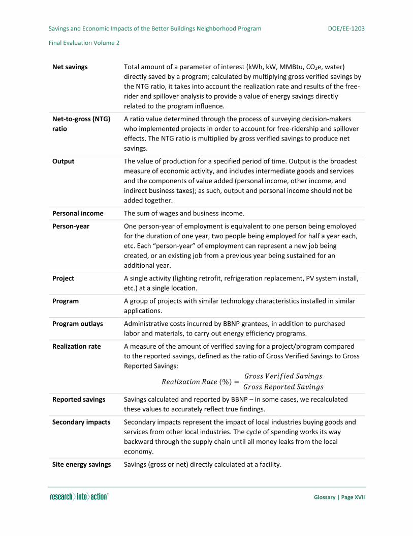
Within the body of this report, there are several technical terms that require explanation. Additionally,
some of the terms may appear to be similar at first review; however, they have very different meanings.
Terms such as “site” and “source” can easily be confused by the reader and are thus defined in this
glossary.
Adjustment factor A value that allows the billing analysis and monitoring and verification (M&V)
work to be merged. The adjustment factor was created to address the
concern of differing baselines between these two impact evaluation
methodologies The billing analysis utilizes existing conditions as the baseline
for all energy savings impacts, while the M&V analysis adjusts the baseline for
building energy codes or energy efficiency standards.
Base case/
counterfactual
scenario
Describes what would have happened in the absence of the program.
Baseline The expected energy usage level of a specific measure or project before
improvements are implemented. This becomes the comparison value for all
energy savings calculations.
Benefit-cost ratio The ratio of program economic benefits (defined as the sum of net economic
output and tax revenues) to program costs.
Billing regression Billing analysis that involves the use of regression models with historical utility
billing data to calculate annual energy savings.
Business income Payments received by small-business owners or self-employed workers;
income received by private business owners including doctors, accountants,
lawyers, and others. Also called “proprietor income” or “small business
income.” See “personal income.”
Cooling degree days
(CDD)
The number of degrees that a day's average temperature is above 65°
Fahrenheit, the temperature below which buildings need to be cooled.
Deemed savings Amount of savings for a particular measure provided by documented and
validated sources or reference materials. Often used when confidence is high
for a specific measure, databases lack sufficient information, or costs of
measurement and verification greatly outweigh the benefits.
Direct impacts Direct impacts represent the initial set of expenditures applied to the
predictive model for impact analysis, which result in additional, secondary
impacts as the industries affected directly purchase intermediate goods and
services, and employee additional labor.
Savings and Economic Impacts of the Better Buildings Neighborhood Program DOE/EE-1203
Final Evaluation Volume 2
Glossary | Page XVI
Dummy variable Also known as a binary variable, dummy variables either take on a value of
zero or one to indicate the state of the data point (that is, either it does or
does not meet the condition).
Fixed effects model The fixed effects model is a model specification that incorporates non-
random, time-invariant explanatory variables in the traditional multivariate
regression framework. These constant terms help control for possible
influences relating to individual cohorts and time periods that are not
controlled for explicitly in the available data. By controlling for these
influences using these additional constant terms, the fixed effects model
provides a more robust estimation of changes in energy use over time.
Free-rider A participant who on some level may have used the program regardless of the
BBNP influence. Determining free-ridership values is a large component in
calculating net-to-gross ratio.
Gross impacts Overall impacts traced back to the program. As they do not constitute an
estimate of the new or additive impacts from BBNP funding over and above
what would have accrued had the funds been used by other federal programs,
gross impacts represent an upper bound estimate and net impacts, which
account for this next best use of program funds by way of a counterfactual or
base case scenario, represent a lower bound estimate.
Gross savings Total amount of a parameter of interest (kWh, kW, MMBtu, CO2e, water)
saved by a project/program.
Heating degree days
(HDD)
The number of degrees that a day's average temperature is below 65°
Fahrenheit, the temperature below which buildings need to be heated.
Input-output model A static model that measures the flow of inputs and outputs in an economy at
a point in time.
Interaction variable A variable that combines two or more variables to represent the interaction
present.
Job Impacts Includes both full- and part-time employment measured in full-time
equivalent (FTE) units.
Measure spending Represents spending on efficiency upgrades; allocated to equipment and
labor, mapped to North American Industry Classification System (NAICS) codes
and then to sectors in the economic impact model.
Net economic
impacts
Counts only economic stimuli that are new or additive to the economy. (See
the definition of gross impacts, above, for an elaboration of how net impacts
differ from gross impacts and of net savings, below, for an application of the
“net” concept to program energy savings.)
Savings and Economic Impacts of the Better Buildings Neighborhood Program DOE/EE-1203
Final Evaluation Volume 2
Glossary | Page XVII
Net savings Total amount of a parameter of interest (kWh, kW, MMBtu, CO2e, water)
directly saved by a program; calculated by multiplying gross verified savings by
the NTG ratio, it takes into account the realization rate and results of the free-
rider and spillover analysis to provide a value of energy savings directly
related to the program influence.
Net-to-gross (NTG)
ratio
A ratio value determined through the process of surveying decision-makers
who implemented projects in order to account for free-ridership and spillover
effects. The NTG ratio is multiplied by gross verified savings to produce net
savings.
Output The value of production for a specified period of time. Output is the broadest
measure of economic activity, and includes intermediate goods and services
and the components of value added (personal income, other income, and
indirect business taxes); as such, output and personal income should not be
added together.
Personal income The sum of wages and business income.
Person-year One person-year of employment is equivalent to one person being employed
for the duration of one year, two people being employed for half a year each,
etc. Each “person-year” of employment can represent a new job being
created, or an existing job from a previous year being sustained for an
additional year.
Project A single activity (lighting retrofit, refrigeration replacement, PV system install,
etc.) at a single location.
Program A group of projects with similar technology characteristics installed in similar
applications.
Program outlays Administrative costs incurred by BBNP grantees, in addition to purchased
labor and materials, to carry out energy efficiency programs.
Realization rate A measure of the amount of verified saving for a project/program compared
to the reported savings, defined as the ratio of Gross Verified Savings to Gross
Reported Savings:
𝑅𝑒𝑎𝑙𝑖𝑧𝑎𝑡𝑖𝑜𝑛 𝑅𝑎𝑡𝑒 (%) = 𝐺𝑟𝑜𝑠𝑠 𝑉𝑒𝑟𝑖𝑓𝑖𝑒𝑑 𝑆𝑎𝑣𝑖𝑛𝑔𝑠
𝐺𝑟𝑜𝑠𝑠 𝑅𝑒𝑝𝑜𝑟𝑡𝑒𝑑 𝑆𝑎𝑣𝑖𝑛𝑔𝑠
Reported savings Savings calculated and reported by BBNP – in some cases, we recalculated
these values to accurately reflect true findings.
Secondary impacts Secondary impacts represent the impact of local industries buying goods and
services from other local industries. The cycle of spending works its way
backward through the supply chain until all money leaks from the local
economy.
Site energy savings Savings (gross or net) directly calculated at a facility.
Savings and Economic Impacts of the Better Buildings Neighborhood Program DOE/EE-1203
Final Evaluation Volume 2
Glossary | Page XVIII
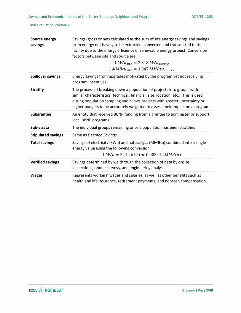
Source energy
savings
Savings (gross or net) calculated as the sum of site energy savings and savings
from energy not having to be extracted, converted and transmitted to the
facility due to the energy efficiency or renewable energy project. Conversion
factors between site and source are:
1 𝑘𝑊ℎ𝑠𝑖𝑡𝑒 = 3.318 𝑘𝑊ℎ𝑠𝑜𝑢𝑟𝑐𝑒
1 𝑀𝑀𝐵𝑡𝑢𝑠𝑖𝑡𝑒 = 1.047 𝑀𝑀𝐵𝑡𝑢𝑠𝑜𝑢𝑟𝑐𝑒
Spillover savings Energy savings from upgrades motivated by the program yet not receiving
program incentives.
Stratify The process of breaking down a population of projects into groups with
similar characteristics (technical, financial, size, location, etc.). This is used
during population sampling and allows projects with greater uncertainty or
higher budgets to be accurately weighted to assess their impact on a program.
Subgrantee An entity that received BBNP funding from a grantee to administer or support
local BBNP programs.
Sub-strata The individual groups remaining once a population has been stratified.
Stipulated savings Same as Deemed Savings
Total savings Savings of electricity (kWh) and natural gas (MMBtu) combined into a single
energy value using the following conversion:
1 𝑘𝑊ℎ = 3412 𝐵𝑡𝑢 (𝑜𝑟 0.003412 𝑀𝑀𝐵𝑡𝑢)
Verified savings Savings determined by we through the collection of data by onsite
inspections, phone surveys, and engineering analysis.
Wages Represents workers’ wages and salaries, as well as other benefits such as
health and life insurance, retirement payments, and noncash compensation.

Savings and Economic Impacts of the Better Buildings Neighborhood Program DOE/EE-1203
Final Evaluation Volume 2
Preface | Page XIX
PREFACE
This evaluation report is one of a suite of seven reports providing a final evaluation of the U.S.
Department of Energy’s (DOE) Better Buildings Neighborhood Program (BBNP). The evaluation was
conducted under contract to Lawrence Berkeley National Laboratory (LBNL) as a procurement under
LBNL Contract No. DE-AC02-05CH11231 with DOE.
The suite of evaluation reports comprises:
Evaluation of the Better Buildings Neighborhood Program (Final Synthesis Report, Volume 1)
Savings and Economic Impacts of the Better Buildings Neighborhood Program (Final Evaluation
Volume 2)
Drivers of Success in the Better Buildings Neighborhood Program – Statistical Process Evaluation
(Final Evaluation Volume 3)
Process Evaluation of the Better Buildings Neighborhood Program (Final Evaluation Volume 4)
Market Effects of the Better Buildings Neighborhood Program (Final Evaluation Volume 5)
Spotlight on Key Program Strategies from the Better Buildings Neighborhood Program (Final
Evaluation Volume 6)
The evaluation commenced in late 2011 and concluded in mid-2015. The evaluation issued two
preliminary reports:
Preliminary Process and Market Evaluation: Better Buildings Neighborhood Program (December
28, 2012; appendices in a separate volume) (Research Into Action and NMR Group, 2012a,
2012b)
Preliminary Energy Savings Impact Evaluation: Better Buildings Neighborhood Program
(November 4, 2013) (Research Into Action, Evergreen Economics, Nexant, and NMR Group,
2013)
Four firms conducted the multi-faceted evaluation:
Research Into Action, Inc. led the teams and process evaluation research.
Evergreen Economics conducted the analysis of economic impacts, the billing regression analysis
of program savings, and worked with Nexant to estimate program savings.
Nexant, Inc. led the impact evaluation, conducted project measurement and verification (M&V)
activities, and estimated program savings and carbon emission reductions.
NMR Group, Inc. led the market effects assessment.
LBNL managed the evaluation; DOE supported it.

Savings and Economic Impacts of the Better Buildings Neighborhood Program DOE/EE-1203
Final Evaluation Volume 2
Preface | Page XX
This document is Savings and Economic Impacts of the Better Buildings Neighborhood Program. Nexant
and Evergreen Economics were the principal author and evaluator, supported in both roles by Research
Into Action.
The Nexant team was led by Lynn Roy, supported by Wyley Hodgson, Cherlyn Seruto, Laura Ruff, and
Andrew Dionne.
The Evergreen Economics team was led by Stephen Grover, supported by Matt Koson, Sarah Monohon,
and John Cornwell.
The Research Into Action team was led by Jane S. Peters and Marjorie McRae, supported by Joe Van
Clock, Jordan Folks, Jun Suzuki, and Meghan Bean. Amber Stadler and Sara Titus provided production
support.

Savings and Economic Impacts of the Better Buildings Neighborhood Program DOE/EE-1203
Final Evaluation Volume 2
Executive Summary | Page ES-1
EXECUTIVE SUMMARY
The U.S. Department of Energy (DOE) administered the Better Buildings Neighborhood Program (BBNP)
to support programs promoting whole building energy upgrades. BBNP distributed a total of $508
million to support efforts in hundreds of communities served by 41 grantees. DOE awarded funding of
$1.4 million to $40 million per grantee through the competitive portions of the Energy Efficiency and
Conservation Block Grant (EECBG) Program ($482 million from American Recovery and Reinvestment
Act of 2009 [ARRA, the Recovery Act] funds) and the State Energy Program (SEP; $26 million). DOE
awarded grants between May and October 2010, intended to provide funding over a three-year period
ending September 30, 2013. In 2013, DOE offered an extension to programs that included a BBNP-
funded financing mechanism to operate through September 30, 2014, using BBNP funds exclusively for
financing.
While the federal government has issued periodic funding opportunities for energy efficiency, none has
been on the scale of BBNP.
State and local governments received the grants and worked with nonprofits, building energy efficiency
experts, contractor trade associations, financial institutions, utilities, and other organizations to develop
community-based programs, incentives, and financing options for comprehensive energy-saving
upgrades. Each of the 41 grant-funded organizations, assisted by 24 subgrantees, targeted a unique
combination of residential, multifamily, commercial, industrial, and agriculture sector buildings,
depending on their objectives.
This report provides the impact findings from a comprehensive impact, process, and market effects
evaluation of the original grantee program period, spanning fourth quarter (Q4) 2010 through third
quarter (Q3) 2013. A team of four energy efficiency evaluation consulting firms conducted the
evaluation – Research Into Action, Inc. (lead contractor), Evergreen Economics, Nexant, Inc., and NMR
Group, Inc. – which was managed by Lawrence Berkeley National Laboratory (LBNL) and supported by
DOE. Nexant led the impact research, with principal support provided by Evergreen Economics and
additional support provided by the two other firms. The study constitutes one report among a suite of
six evaluation reports assessing BBNP.
EVALUATION OBJECTIVES AND METHODS
To assess whether BBNP was successful in meeting its goals and objectives, this study developed
independent, quantitative estimates of the impacts of the BBNP. These impacts include energy and bill
savings and carbon emission reductions for projects installed during the three-year BBNP, as well as
economic impacts such as jobs generated. Based on the investigation and findings, we provide lessons
learned and recommendations to DOE and the grantees are continuing their programs after the grant
funding has ended.
The impact evaluation comprised two broad activities to determine gross verified savings:
Measurement and Verification (M&V) of a sample of grantees and projects
Billing regression analysis on projects from grantees with sufficient utility bill data
Savings and Economic Impacts of the Better Buildings Neighborhood Program DOE/EE-1203
Final Evaluation Volume 2
Executive Summary | Page ES-2
Our M&V approach used an ex-post analysis (actual savings based on post-retrofit conditions) in order
to estimate the energy savings for each project in a representative sample selected to provide high
confidence and precision. We determined gross verified energy savings through: 1) participant onsite
inspections and surveys; 2) review of project files and documentation; and 3) engineering analysis of
projects. We compared gross verified savings to reported savings to determine a realization rate for
each sector with the exception of the agriculture sector due to a small amount of activity and a lack of
available data.
We conducted a billing regression analysis to estimate realized energy savings at the project level. We
reviewed all billing data that grantees provided to DOE and determined that 19 grantees had provided
sufficient data to support regression analysis. We needed both participant billing (monthly electricity or
natural gas consumption before and after program participation) and participant tracking data (for
example, information on when measures were installed).
We quantified impact metrics for the entire three-year BBNP grant cycle based on findings from
preliminary and final evaluations. The preliminary evaluation assessed a sample of projects reported
between Quarter 4 2010 and Quarter 2 2012 (inclusive). The final evaluation verified grantee reported
activities and quantified metrics for a sample of projects reported between Quarter 3 (Q3) of 2012 and
Quarter 3 (Q3) of 2013. We conducted the preliminary research and analysis from January 2013 through
May 2013; we conducted the final research and analysis from December 2013 to October 2014.
In order to calculate the overall verified energy savings associated with BBNP, the team extrapolated the
sample findings to the population through the use of case weights and realization rates. Due to the
intrinsic differences in baseline conditions between the M&V analysis and billing regression analysis, we
developed an adjustment factor based on a subset of overlapping projects between each analysis (see
section 3.4). This adjustment factor was applied to the savings estimates of the billing regression
analysis to make the savings estimates comparable to the M&V savings estimates. We then extrapolated
the M&V sample frame and the billing regression analysis sample frame separately, and we combined
the resulting realization rates and extrapolated to the entire BBNP. Finally, we calculated and applied a
net-to-gross (NTG) ratio estimated from survey research to the extrapolated savings to estimate BBNP’s
total net energy savings.
The impact evaluation also estimated the economic impacts of BBNP. These impacts included jobs as
well as estimates of economic output, income (personal and business), and tax revenue that result from
the program spending relative to a base case scenario where BBNP did not exist.
BBNP GOALS AND OBJECTIVES
DOE designed BBNP to meet the three principal ARRA goals (Table ES-1), as well as seven objectives
developed by DOE staff to guide the BBNP initiative (Table ES-2). Below, we identify which of the three
types of evaluation (impact, process, or market effects) provide findings relevant to our assessment of
goal and objective attainment. This study addresses the goals and objectives flagged in the tables as
relating to the impact evaluation. For an investigation of the other goals and objectives noted in the
tables, see the companion reports Process Evaluation of the Better Buildings Neighborhood Program

Savings and Economic Impacts of the Better Buildings Neighborhood Program DOE/EE-1203
Final Evaluation Volume 2
Executive Summary | Page ES-3
(Final Evaluation Volume 4), and Market Effects of the Better Buildings Neighborhood Program (Final
Evaluation Volume 5).
Table ES-1: ARRA Goals
GOALS
EVALUATION TYPE
Impact Process Market Effects
Create new jobs and save existing ones
Spur economic activity and invest in long-term growth
Provide accountability and transparency in spending BBNP funds
Table ES-2: BBNP Objectives
OBJECTIVES
EVALUATION TYPE
Impact Process Market Effects
Develop sustainable energy efficiency upgrade programs
Upgrade more than 100,000 residential and commercial buildings to be more
energy efficient
Save consumers $65 million annually on their energy bills
Achieve 15% to 30% estimated energy savings from residential energy efficiency
upgrades
Reduce the cost of energy efficiency program delivery by 20% or more
Create or retain 10,000 to 30,000 jobs
Leverage $1 to $3 billion in additional resources
GOAL AND OBJECTIVE ATTAINMENT
By the end of the three-year evaluation period (Q4 2010 to Q3 2013) BBNP had met the three ARRA
goals, as shown in Table ES-3, which presents our findings, including net jobs, net economic activity, and
net benefit-cost ratio. For the economic metrics, the term “net” signifies BBNP’s contribution to these
outcomes above and beyond the outcomes that would have occurred had the BBNP funding been spent
according to historical non-defense federal spending patterns.
By the end of the three-year evaluation period, BBNP met two of the five impact-related BBNP
objectives (Table ES-4). Unverified program-reported accomplishments for Q4 2013 through Q3 2014
suggest the program likely was successful in meeting four of the five impact-related objectives by the

Savings and Economic Impacts of the Better Buildings Neighborhood Program DOE/EE-1203
Final Evaluation Volume 2
Executive Summary | Page ES-4
end of the four-year program period. These findings indicate that BBNP met its objectives to spur energy
efficiency upgrade activity, achieve energy savings, and create or maintain jobs.
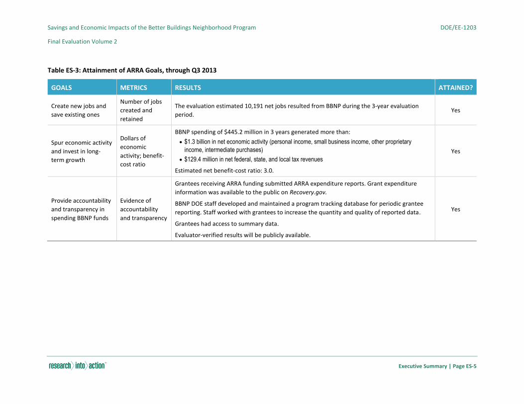
Savings and Economic Impacts of the Better Buildings Neighborhood Program DOE/EE-1203
Final Evaluation Volume 2
Executive Summary | Page ES-5
Table ES-3: Attainment of ARRA Goals, through Q3 2013
GOALS METRICS RESULTS ATTAINED?
Create new jobs and
save existing ones
Number of jobs
created and
retained
The evaluation estimated 10,191 net jobs resulted from BBNP during the 3-year evaluation
period. Yes
Spur economic activity
and invest in long-
term growth
Dollars of
economic
activity; benefit-
cost ratio
BBNP spending of $445.2 million in 3 years generated more than:
$1.3 billion in net economic activity (personal income, small business income, other proprietary
income, intermediate purchases)
$129.4 million in net federal, state, and local tax revenues
Estimated net benefit-cost ratio: 3.0.
Yes
Provide accountability
and transparency in
spending BBNP funds
Evidence of
accountability
and transparency
Grantees receiving ARRA funding submitted ARRA expenditure reports. Grant expenditure
information was available to the public on Recovery.gov.
BBNP DOE staff developed and maintained a program tracking database for periodic grantee
reporting. Staff worked with grantees to increase the quantity and quality of reported data.
Grantees had access to summary data.
Evaluator-verified results will be publicly available.
Yes
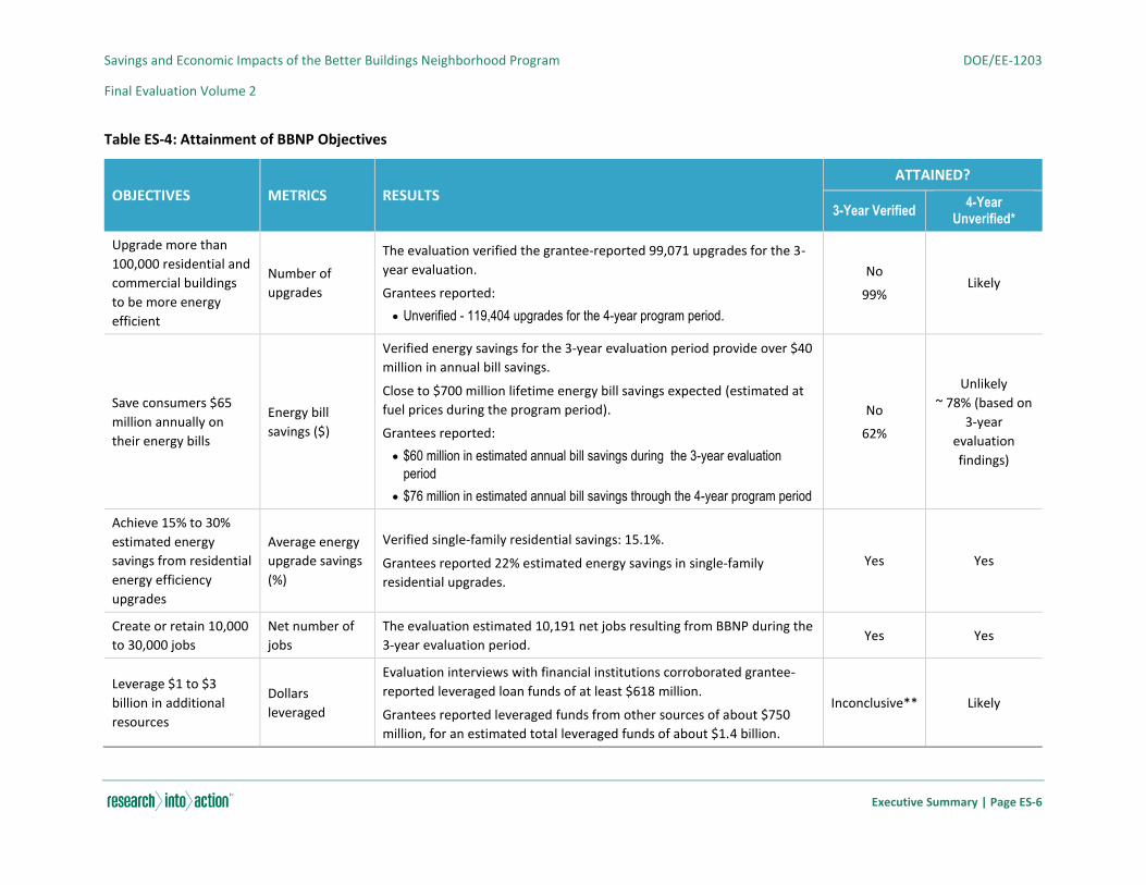
Savings and Economic Impacts of the Better Buildings Neighborhood Program DOE/EE-1203
Final Evaluation Volume 2
Executive Summary | Page ES-6
Table ES-4: Attainment of BBNP Objectives
OBJECTIVES METRICS RESULTS
ATTAINED?
3-Year Verified 4-Year
Unverified*
Upgrade more than
100,000 residential and
commercial buildings
to be more energy
efficient
Number of
upgrades
The evaluation verified the grantee-reported 99,071 upgrades for the 3-
year evaluation.
Grantees reported:
Unverified - 119,404 upgrades for the 4-year program period.
No
99% Likely
Save consumers $65
million annually on
their energy bills
Energy bill
savings ($)
Verified energy savings for the 3-year evaluation period provide over $40
million in annual bill savings.
Close to $700 million lifetime energy bill savings expected (estimated at
fuel prices during the program period).
Grantees reported:
$60 million in estimated annual bill savings during the 3-year evaluation
period
$76 million in estimated annual bill savings through the 4-year program period
No
62%
Unlikely
~ 78% (based on
3-year
evaluation
findings)
Achieve 15% to 30%
estimated energy
savings from residential
energy efficiency
upgrades
Average energy
upgrade savings
(%)
Verified single-family residential savings: 15.1%.
Grantees reported 22% estimated energy savings in single-family
residential upgrades.
Yes Yes
Create or retain 10,000
to 30,000 jobs
Net number of
jobs
The evaluation estimated 10,191 net jobs resulting from BBNP during the
3-year evaluation period. Yes Yes
Leverage $1 to $3
billion in additional
resources
Dollars
leveraged
Evaluation interviews with financial institutions corroborated grantee-
reported leveraged loan funds of at least $618 million.
Grantees reported leveraged funds from other sources of about $750
million, for an estimated total leveraged funds of about $1.4 billion.
Inconclusive** Likely

Savings and Economic Impacts of the Better Buildings Neighborhood Program DOE/EE-1203
Final Evaluation Volume 2
Executive Summary | Page ES-7
* Our evaluation did not verify fourth-year program achievements. We concluded that objectives that were met by Q3 2013 also were met by the end of Q3 2014. An assessment
of “likely” indicates that the unverified data show a trend suggestive of achievement.
** The evaluation addressed financial leverage amounts only; it did not address other grantee-reported leveraged funds.
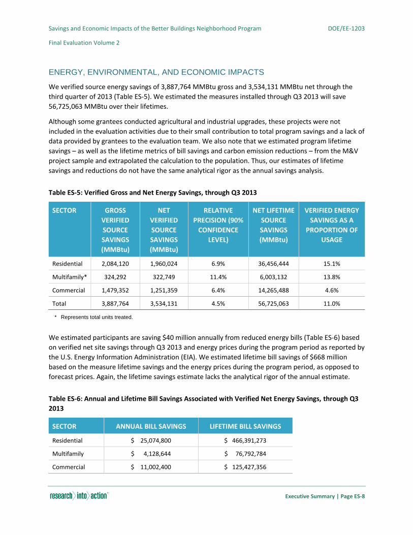
Savings and Economic Impacts of the Better Buildings Neighborhood Program DOE/EE-1203
Final Evaluation Volume 2
Executive Summary | Page ES-8
ENERGY, ENVIRONMENTAL, AND ECONOMIC IMPACTS
We verified source energy savings of 3,887,764 MMBtu gross and 3,534,131 MMBtu net through the
third quarter of 2013 (Table ES-5). We estimated the measures installed through Q3 2013 will save
56,725,063 MMBtu over their lifetimes.
Although some grantees conducted agricultural and industrial upgrades, these projects were not
included in the evaluation activities due to their small contribution to total program savings and a lack of
data provided by grantees to the evaluation team. We also note that we estimated program lifetime
savings – as well as the lifetime metrics of bill savings and carbon emission reductions – from the M&V
project sample and extrapolated the calculation to the population. Thus, our estimates of lifetime
savings and reductions do not have the same analytical rigor as the annual savings analysis.
Table ES-5: Verified Gross and Net Energy Savings, through Q3 2013
SECTOR GROSS
VERIFIED
SOURCE
SAVINGS
(MMBtu)
NET
VERIFIED
SOURCE
SAVINGS
(MMBtu)
RELATIVE
PRECISION (90%
CONFIDENCE
LEVEL)
NET LIFETIME
SOURCE
SAVINGS
(MMBtu)
VERIFIED ENERGY
SAVINGS AS A
PROPORTION OF
USAGE
Residential 2,084,120 1,960,024 6.9% 36,456,444 15.1%
Multifamily* 324,292 322,749 11.4% 6,003,132 13.8%
Commercial 1,479,352 1,251,359 6.4% 14,265,488 4.6%
Total 3,887,764 3,534,131 4.5% 56,725,063 11.0%
* Represents total units treated.
We estimated participants are saving $40 million annually from reduced energy bills (Table ES-6) based
on verified net site savings through Q3 2013 and energy prices during the program period as reported by
the U.S. Energy Information Administration (EIA). We estimated lifetime bill savings of $668 million
based on the measure lifetime savings and the energy prices during the program period, as opposed to
forecast prices. Again, the lifetime savings estimate lacks the analytical rigor of the annual estimate.
Table ES-6: Annual and Lifetime Bill Savings Associated with Verified Net Energy Savings, through Q3
2013
SECTOR ANNUAL BILL SAVINGS LIFETIME BILL SAVINGS
Residential $ 25,074,800 $ 466,391,273
Multifamily $ 4,128,644 $ 76,792,784
Commercial $ 11,002,400 $ 125,427,356
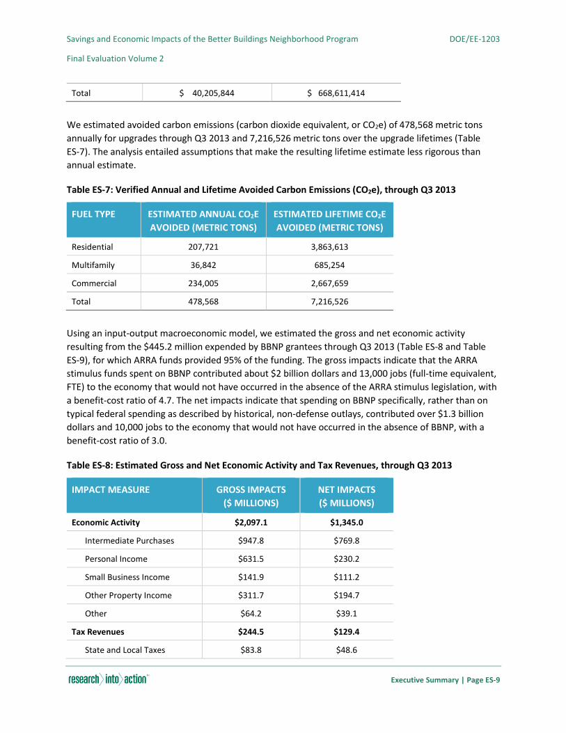
Savings and Economic Impacts of the Better Buildings Neighborhood Program DOE/EE-1203
Final Evaluation Volume 2
Executive Summary | Page ES-9
Total $ 40,205,844 $ 668,611,414
We estimated avoided carbon emissions (carbon dioxide equivalent, or CO2e) of 478,568 metric tons
annually for upgrades through Q3 2013 and 7,216,526 metric tons over the upgrade lifetimes (Table
ES-7). The analysis entailed assumptions that make the resulting lifetime estimate less rigorous than
annual estimate.
Table ES-7: Verified Annual and Lifetime Avoided Carbon Emissions (CO2e), through Q3 2013
FUEL TYPE ESTIMATED ANNUAL CO2E
AVOIDED (METRIC TONS)
ESTIMATED LIFETIME CO2E
AVOIDED (METRIC TONS)
Residential 207,721 3,863,613
Multifamily 36,842 685,254
Commercial 234,005 2,667,659
Total 478,568 7,216,526
Using an input-output macroeconomic model, we estimated the gross and net economic activity
resulting from the $445.2 million expended by BBNP grantees through Q3 2013 (Table ES-8 and Table
ES-9), for which ARRA funds provided 95% of the funding. The gross impacts indicate that the ARRA
stimulus funds spent on BBNP contributed about $2 billion dollars and 13,000 jobs (full-time equivalent,
FTE) to the economy that would not have occurred in the absence of the ARRA stimulus legislation, with
a benefit-cost ratio of 4.7. The net impacts indicate that spending on BBNP specifically, rather than on
typical federal spending as described by historical, non-defense outlays, contributed over $1.3 billion
dollars and 10,000 jobs to the economy that would not have occurred in the absence of BBNP, with a
benefit-cost ratio of 3.0.
Table ES-8: Estimated Gross and Net Economic Activity and Tax Revenues, through Q3 2013
IMPACT MEASURE GROSS IMPACTS
($ MILLIONS)
NET IMPACTS
($ MILLIONS)
Economic Activity $2,097.1 $1,345.0
Intermediate Purchases $947.8 $769.8
Personal Income $631.5 $230.2
Small Business Income $141.9 $111.2
Other Property Income $311.7 $194.7
Other $64.2 $39.1
Tax Revenues $244.5 $129.4
State and Local Taxes $83.8 $48.6

Savings and Economic Impacts of the Better Buildings Neighborhood Program DOE/EE-1203
Final Evaluation Volume 2
Executive Summary | Page ES-10
IMPACT MEASURE GROSS IMPACTS
($ MILLIONS)
NET IMPACTS
($ MILLIONS)
Federal Taxes $160.7 $80.8
Table ES-9: Estimated Gross and Net Benefit-Cost Ration and Jobs Impact, through Q3 2013
IMPACT MEASURE TOTAL GROSS IMPACTS TOTAL NET IMPACTS
Benefit-Cost Ratio 4.71 3.02
Jobs (FTE) 13,331 10,191
IMPACT ASSESSMENT LESSONS LEARNED
The main objective of this impact evaluation was to determine the impacts of $508 million in BBNP
spending that allocated resources to varied energy efficiency programs across the country. The
challenges associated with this task, such as difficulty in acquiring grantee data, lack of quality
control/assurance leading to inaccuracies of reported metrics, and the large scale and broad scope of
grantee programs, affected the team’s evaluation activities. While navigating these challenges, we
learned many lessons that will help shape the future of similar program evaluations. Key among these
lessons are:
Allow sufficient time to request and gather data from the grantees. Grantees are busy, and
unlike most utility-funded efficiency program managers, they are not equipped with the tools
and databases to easily extract participant and project level information. In addition, grantees
are frequently understaffed, so making clear and concise data requests are necessary to help
speed up the response time and alleviate any concerns or questions that they may have
regarding data needs.
Phone verifications had limited value. Phone verifications are standard practice in many utility-
funded impact evaluations. While the phone surveys were useful in verifying overall project
participation and obtaining information on program influence, we determined during the
preliminary evaluation that the phone verifications used for M&V often provided limited value.
The majority of participants interviewed had difficulty remembering the specifics surrounding
completed upgrades, and gathering key data on measures implemented. This is likely due to the
long timespan (averaging one to two years) between measure installation and phone
verifications. There also was confusion among participants regarding the measure funding
source (BBNP or local utility program).
Onsite verifications were valuable. While onsite surveys encounter some of the same issues
with reliability as the phone surveys, the onsite surveys were valuable in obtaining a greater
level of detail regarding project implementation than could be obtained during phone
verifications and file review.

Savings and Economic Impacts of the Better Buildings Neighborhood Program DOE/EE-1203
Final Evaluation Volume 2
Executive Summary | Page ES-11
RECOMMENDATIONS
The grant cycle for BBNP has ended, and it is unlikely that in the foreseeable future DOE will fund a
program on a scale similar to BBNP. Were DOE or another agency to fund a program like BBNP, we offer
the following recommendations to foster greater consistency in program expectations, design, tracking,
and reporting:
Plan and develop a comprehensive and easy to use data tracking and reporting system available
to grantees at time of funding award.
Require grantees to ensure the consistency of project-level tracking values with overall quarterly
report values.
Require consistent documentation procedures across all grantees and programs.
Require accountability for quality control practices across programs.
Provide support to grantees that may demonstrate insufficient quality assurance/quality control
and provide support to grantees that may demonstrate insufficient quality assurance/quality
control.
Consider a requirement of timely and accurate progress reports as a condition of funding
payments.
Compile a single final dataset to be used for reporting and evaluation purposes.

Savings and Economic Impacts of the Better Buildings Neighborhood Program DOE/EE-1203
Final Evaluation Volume 2
Introduction | Page 1
1. INTRODUCTION
The U.S. Department of Energy (DOE) administered the Better Buildings Neighborhood Program (BBNP)
to support programs promoting whole building energy upgrades. BBNP distributed a total of $508
million to support hundreds of communities served by 41 grantees. DOE awarded funding of $1.4 million
to $40 million per grantee through the competitive portions of the Energy Efficiency and Conservation
Block Grant (EECBG) Program ($482 million in American Recovery and Reinvestment Act [ARRA, the
Recovery Act] of 2009 funds) and the State Energy Program (SEP; $26 million). DOE awarded grants
between May and October 2010 intended to provide funding over a three-year period ending
September 30, 2013. In 2013, DOE offered an extension to ARRA-funded grantees with ongoing
financing programs to operate through September 30, 2014, using BBNP funds exclusively for financing.
State and local governments received the grants and worked with nonprofits, building energy efficiency
experts, contractor trade associations, financial institutions, utilities, and other organizations to develop
community-based programs, incentives, and financing options for comprehensive energy saving
upgrades. Each of the 41 grant-funded organizations, assisted by 24 subgrantees, targeted a unique
combination of residential, multifamily, commercial, industrial, and agriculture sector buildings,
depending on their objectives.
This report provides the impact findings from a comprehensive impact, process, and market effects
evaluation of the original program period spanning fourth quarter (Q4) 2010 through third quarter (Q3)
2013. A team of four energy efficiency evaluation consulting firms conducted the comprehensive
evaluation – Research Into Action, Inc. (lead contractor), Evergreen Economics, Nexant, Inc., and NMR
Group, Inc. – which was managed by Lawrence Berkeley National Laboratory (LBNL) and supported by
DOE. Nexant led the impact research, with principal support provided by Evergreen Economics and
additional support provided by the other two firms. The study constitutes one report among a suite of
six evaluation reports assessing BBNP.
1.1. STUDY OVERVIEW
To assess whether BBNP was successful in meeting its goals and objectives, this study developed
independent, quantitative estimates of the impacts of the BBNP. These impacts include energy savings,
cost savings, greenhouse gas emission reductions, economic impacts, and jobs created or maintained for
projects installed during the three-year BBNP. Based on the investigation and findings, we provide
lessons learned and recommendations to DOE and the grantees that wish to continue their programs
after the grant funding has ended.
The impact evaluation comprised two broad activities to determine gross verified savings: 1)
Measurement and Verification (M&V) of a sample of grantees and projects, using an ex-post analysis
(actual savings based on post-retrofit conditions); and 2) billing regression analysis on projects from
grantees with sufficient utility bill data. The impact evaluation also constructed an economic impact
model of the U.S. economy and estimated the economic impacts of BBNP, including jobs, economic
output, income (personal and business), and tax revenue that result from the program spending relative
to a base case scenario where BBNP does not exist.
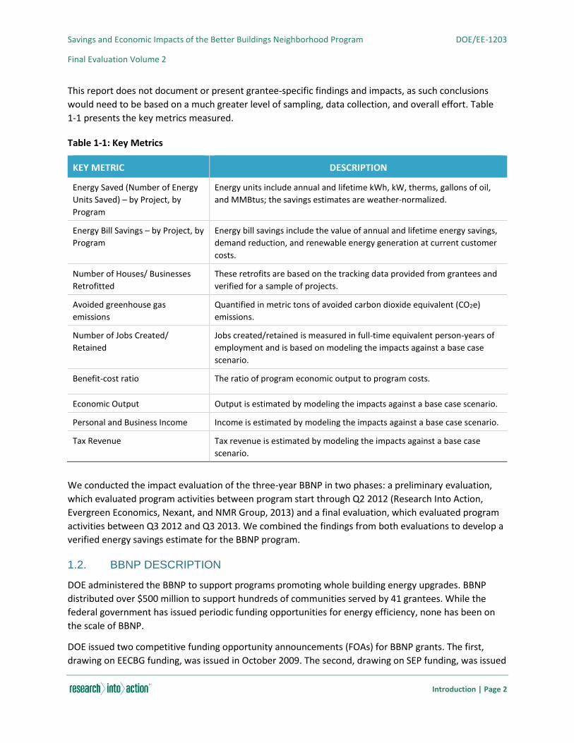
Savings and Economic Impacts of the Better Buildings Neighborhood Program DOE/EE-1203
Final Evaluation Volume 2
Introduction | Page 2
This report does not document or present grantee-specific findings and impacts, as such conclusions
would need to be based on a much greater level of sampling, data collection, and overall effort. Table
1-1 presents the key metrics measured.
Table 1-1: Key Metrics
KEY METRIC DESCRIPTION
Energy Saved (Number of Energy
Units Saved) – by Project, by
Program
Energy units include annual and lifetime kWh, kW, therms, gallons of oil,
and MMBtus; the savings estimates are weather-normalized.
Energy Bill Savings – by Project, by
Program
Energy bill savings include the value of annual and lifetime energy savings,
demand reduction, and renewable energy generation at current customer
costs.
Number of Houses/ Businesses
Retrofitted
These retrofits are based on the tracking data provided from grantees and
verified for a sample of projects.
Avoided greenhouse gas
emissions
Quantified in metric tons of avoided carbon dioxide equivalent (CO2e)
emissions.
Number of Jobs Created/
Retained
Jobs created/retained is measured in full-time equivalent person-years of
employment and is based on modeling the impacts against a base case
scenario.
Benefit-cost ratio The ratio of program economic output to program costs.
Economic Output Output is estimated by modeling the impacts against a base case scenario.
Personal and Business Income Income is estimated by modeling the impacts against a base case scenario.
Tax Revenue Tax revenue is estimated by modeling the impacts against a base case
scenario.
We conducted the impact evaluation of the three-year BBNP in two phases: a preliminary evaluation,
which evaluated program activities between program start through Q2 2012 (Research Into Action,
Evergreen Economics, Nexant, and NMR Group, 2013) and a final evaluation, which evaluated program
activities between Q3 2012 and Q3 2013. We combined the findings from both evaluations to develop a
verified energy savings estimate for the BBNP program.
1.2. BBNP DESCRIPTION
DOE administered the BBNP to support programs promoting whole building energy upgrades. BBNP
distributed over $500 million to support hundreds of communities served by 41 grantees. While the
federal government has issued periodic funding opportunities for energy efficiency, none has been on
the scale of BBNP.
DOE issued two competitive funding opportunity announcements (FOAs) for BBNP grants. The first,
drawing on EECBG funding, was issued in October 2009. The second, drawing on SEP funding, was issued

Savings and Economic Impacts of the Better Buildings Neighborhood Program DOE/EE-1203
Final Evaluation Volume 2
Introduction | Page 3
in April 2010. Awarded grants between May and October 2010 were intended to provide funding over a
three-year period ending
September 30, 2013. (During the grant period, DOE determined that programs that included a BBNP-
funded financing mechanism could continue to operate beyond the grant period using BBNP funds
exclusively for financing.)
Each grant recipient proposed and implemented unique programs designed to address the energy
efficiency needs, barriers, and opportunities within its jurisdiction. However, all of the recipients’
programs were broadly designed around three common purposes: 1) to obtain high-quality retrofits
resulting in significant energy improvements (retrofits also described as whole building or
comprehensive); 2) to incorporate a viable strategy for program sustainability, which DOE defined as
continuing beyond the grant period without additional federal funding; and 3) to fundamentally and
permanently transform energy markets to make energy efficiency and renewable energy the options of
first choice (DOE, 2009):
Through the EECBG FOA, DOE sought “innovative, ‘game–changing’ whole-building efficiency programs
(DOE, 2009). DOE recognized that innovation is a form of experimentation and is not without risk of
failure. The BBNP program at that national level was looking to identify the most effective approaches;
DOE was not expecting every local BBNP-funded program to be equally, or even moderately, effective.
DOE provided BBNP grants to 41 recipients operating programs in 32 states and territories. The
jurisdictions recipients served varied widely. Some recipients served only a single city or county, while
others served entire states. One recipient, the Southeast Energy Efficiency Alliance (SEEA), funded sub-
recipient (subgrantee) programs in five states and the U.S. Virgin Islands. The sizes of grants awarded
through BBNP also varied, ranging from $1.3 million to $40 million.
Figure 1-1 shows the states with BBNP activity and illustrates whether the grant recipient represented
the state or a city or county within the state. Appendix A provides tables listing the grantee awards in
descending order by size and alphabetically by grantee.
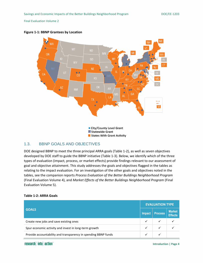
Savings and Economic Impacts of the Better Buildings Neighborhood Program DOE/EE-1203
Final Evaluation Volume 2
Introduction | Page 4
Figure 1-1: BBNP Grantees by Location
1.3. BBNP GOALS AND OBJECTIVES
DOE designed BBNP to meet the three principal ARRA goals (Table 1-2), as well as seven objectives
developed by DOE staff to guide the BBNP initiative (Table 1-3). Below, we identify which of the three
types of evaluation (impact, process, or market effects) provide findings relevant to our assessment of
goal and objective attainment. This study addresses the goals and objectives flagged in the tables as
relating to the impact evaluation. For an investigation of the other goals and objectives noted in the
tables, see the companion reports Process Evaluation of the Better Buildings Neighborhood Program
(Final Evaluation Volume 4), and Market Effects of the Better Buildings Neighborhood Program (Final
Evaluation Volume 5).
Table 1-2: ARRA Goals
GOALS
EVALUATION TYPE
Impact Process Market Effects
Create new jobs and save existing ones
Spur economic activity and invest in long-term growth
Provide accountability and transparency in spending BBNP funds

Savings and Economic Impacts of the Better Buildings Neighborhood Program DOE/EE-1203
Final Evaluation Volume 2
Introduction | Page 5
Table 1-3: BBNP Objectives
OBJECTIVES
EVALUATION TYPE
Impact Process Market Effects
Develop sustainable energy efficiency upgrade programs
Upgrade more than 100,000 residential and commercial buildings to be more
energy efficient
Save consumers $65 million annually on their energy bills
Achieve 15% to 30% estimated energy savings from residential energy efficiency
upgrades
Reduce the cost of energy efficiency program delivery by 20% or more
Create or retain 10,000 to 30,000 jobs
Leverage $1 to $3 billion in additional resources
1.4. PROGRAM TERMINOLOGY
In order to effectively communicate key details of the report and ensure consistency with the process
and market evaluations, the following terminology will be used throughout. The BBNP will refer to the
entire grant program encompassing both EECBG and SEP grants. Grantees will refer to the states,
counties, cities, and organizations that were awarded the funds while sub-grantees are the
organizations or local governments that received funding from the grantees. The grantees are operating
a program with the awarded funding and may have sub-grantees operating programs as well. These
programs encompass a variety of activities including contractor training programs, financing programs,
rebate programs, energy assessments, etc. Participants are the businesses, residents, or contractors
who take part in these programs. A collection of one or more energy upgrade measures that are
implemented by a participant in a home or building is considered a project.
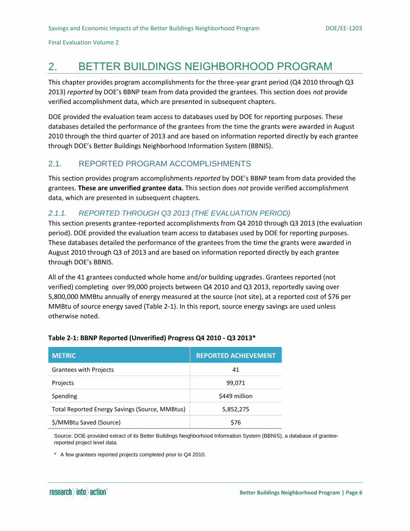
Savings and Economic Impacts of the Better Buildings Neighborhood Program DOE/EE-1203
Final Evaluation Volume 2
Better Buildings Neighborhood Program | Page 6
2. BETTER BUILDINGS NEIGHBORHOOD PROGRAM
This chapter provides program accomplishments for the three-year grant period (Q4 2010 through Q3
2013) reported by DOE’s BBNP team from data provided the grantees. This section does not provide
verified accomplishment data, which are presented in subsequent chapters.
DOE provided the evaluation team access to databases used by DOE for reporting purposes. These
databases detailed the performance of the grantees from the time the grants were awarded in August
2010 through the third quarter of 2013 and are based on information reported directly by each grantee
through DOE’s Better Buildings Neighborhood Information System (BBNIS).
2.1. REPORTED PROGRAM ACCOMPLISHMENTS
This section provides program accomplishments reported by DOE’s BBNP team from data provided the
grantees. These are unverified grantee data. This section does not provide verified accomplishment
data, which are presented in subsequent chapters.
2.1.1. REPORTED THROUGH Q3 2013 (THE EVALUATION PERIOD)
This section presents grantee-reported accomplishments from Q4 2010 through Q3 2013 (the evaluation
period). DOE provided the evaluation team access to databases used by DOE for reporting purposes.
These databases detailed the performance of the grantees from the time the grants were awarded in
August 2010 through Q3 of 2013 and are based on information reported directly by each grantee
through DOE’s BBNIS.
All of the 41 grantees conducted whole home and/or building upgrades. Grantees reported (not
verified) completing over 99,000 projects between Q4 2010 and Q3 2013, reportedly saving over
5,800,000 MMBtu annually of energy measured at the source (not site), at a reported cost of $76 per
MMBtu of source energy saved (Table 2-1). In this report, source energy savings are used unless
otherwise noted.
Table 2-1: BBNP Reported (Unverified) Progress Q4 2010 - Q3 2013*
METRIC REPORTED ACHIEVEMENT
Grantees with Projects 41
Projects 99,071
Spending $449 million
Total Reported Energy Savings (Source, MMBtus) 5,852,275
$/MMBtu Saved (Source) $76
Source: DOE-provided extract of its Better Buildings Neighborhood Information System (BBNIS), a database of grantee-
reported project level data.
* A few grantees reported projects completed prior to Q4 2010.

Savings and Economic Impacts of the Better Buildings Neighborhood Program DOE/EE-1203
Final Evaluation Volume 2
Better Buildings Neighborhood Program | Page 7
Grantees conducted upgrades in the residential, multifamily, commercial/industrial, and agricultural
sectors
(Table 2-2).1, 2, 3 The residential sector accounted for 75% of the projects, but only 51% of the savings.
The commercial sector accounted for less than 4% of the projects, but nearly 38% of the savings.
Table 2-2: BBNP Reported (Unverified) Projects and Energy Savings Q4 2010 - Q3 2013*
SECTOR NUMBER OF
PROJECTS
IMPLEMENTED
PERCENT OF
TOTAL
PROJECTS
TOTAL SOURCE
ENERGY SAVINGS
(MMBtu)
PERCENT OF
PORTFOLIO
SAVINGS
Residential 74,184 74.9% 2,975,346 50.8%
Multifamily 21,178 21.4% 603,432 10.3%
Commercial 3,546 3.6% 2,240,970 38.3%
Agriculture** 163 0.2% 32,526 0.6%
BBNP Total 99,071 100% 5,852,275 100%
Source: DOE-BBNIS.
* A few grantees reported projects completed prior to Q4 2010.
** Agriculture totals obtained from DOE email dated May 9, 2013, as they are not included in Project Level data.
Table 2-3 provides the average project savings for each of the four sectors.
Table 2-3: Average BBNP Reported (Unverified) Savings per Project by Sector
SECTOR AVERAGE SOURCE SAVINGS
PER PROJECT (MMBtu)
Residential 40
Multifamily (individual
units)*
29
Commercial 632
Agriculture 200
1 Industrial projects were limited to 15 upgrades conducted by one grantee.
2 Table 2-2 outlines results as reported from the Project Level database. Throughout the course of the evaluation activities, DOE
adjusted the reporting database to correct for errors in reported data from grantees. The information presented in this table
represents reported values recorded as of September 2014.
3 Grantees reported savings from a number of different fuel types including electricity, natural gas, fuel oil, propane, kerosene,
and wood. In order to convert the savings achieved from these different fuel types to site and source MMBtu savings, the team
used the conversion factors found in Appendix I.
Savings and Economic Impacts of the Better Buildings Neighborhood Program DOE/EE-1203
Final Evaluation Volume 2
Better Buildings Neighborhood Program | Page 8
Source: DOE-BBNIS.
The overall savings reported by the grantees included savings from a variety of fuel types including
electricity, natural gas, fuel oil, propane, kerosene, and wood. Natural gas and electricity savings were
the most common sources of savings. Table 2-4 presents the reported savings per fuel type for each
sector, presented as site savings in the specific fuel units, consistent with DOE’s reporting.
Table 2-4: BBNP Reported (Unverified) Site Energy Savings through Q3 2013 by Fuel Type per Sector
SECTOR ELECTRICITY
(KWH)
NATURAL GAS
(THERMS)
FUEL OIL
(GALLONS)
PROPANE
(GALLONS)
KEROSENE
(GALLONS)
Residential 87,510,900 13,698,543 2,648,021 213,362 5,723
Multifamily 20,681,620 2,498,801 539,016 4,051 —
Commercial 173,940,718 2,004,409 90,170 87,420 —
Agriculture* 2,405,535 13,778 3,607 229,779 —
Total 282,133,238 18,201,753 3,280,814 534,612 5,723
Source: DOE-BBNIS.
* Agriculture totals obtained from DOE email dated May 9, 2013, as they are not included in Project Level data.
Grantees reported savings from a number of different fuel types including electricity, natural gas, fuel
oil, propane, kerosene, and wood. Electricity and natural gas savings were the most common fuel
sources, comprising 92% of the overall reported (unverified) source MMBtu savings (Figure 2-1).
Figure 2-1: Percent of Total BBNP Reported (Unverified) MMBtu Savings by Fuel Type
Source: DOE-BBNIS.
Figure 2-2 and Figure 2-3 illustrate the two major fuel types saved (electricity and natural gas) by sector.
As these figures illustrate, the commercial sector was reported to be responsible for a majority of the
Electricity, 56%
Natural Gas, 35%
Fuel Oil, 8%
Propane, 1%

Savings and Economic Impacts of the Better Buildings Neighborhood Program DOE/EE-1203
Final Evaluation Volume 2
Better Buildings Neighborhood Program | Page 9
electricity (kWh) savings while the residential sector was responsible for the majority of reported natural
gas (therms) savings.
Figure 2-2: Electricity Savings by Sector (kWh)
Figure 2-3: Natural Gas Savings by Sector
(therms)
Upgrade customers most commonly installed heating and/or cooling systems, insulation, and air sealing
measures; these measures comprised 91% of the overall reported (unverified) source MMBtu savings
and 81% of installed measures (Figure 2-4).
Figure 2-4: BBNP Reported Installed Measure Counts
Residential31%
Commercial62%
Residential Multifamily
7%
Residential75%
Commercial11%
Residential Multifamily
14%
31,146 32,636 31,886
13,39310,617
20,631
4,2291,361 1,925
3,541
214
4,432
671396 505
67
173
157
141593 31
2,313
63
703
0
5,000
10,000
15,000
20,000
25,000
30,000
35,000
40,000
InsulationMeasures
Heating and/orCooling
Measures
SealingMeasures
LightingMeasures
Water HeatingMeasures
All OtherMeasures
Commercial
Multifamilybuilding
Multifamily unit
Single-family
Savings and Economic Impacts of the Better Buildings Neighborhood Program DOE/EE-1203
Final Evaluation Volume 2
Better Buildings Neighborhood Program | Page 10
Source: DOE-BBNIS.
2.1.2. REPORTED THROUGH Q3 2014 (THE END OF THE EXTENSION PERIOD)
In 2013, DOE provided an extension to ARRA-funded grantees with ongoing financing programs to
operate through Q3 2014. By the end of this period, grantees reported cumulative spending of $508
million and conducting 115,640 upgrades. The following tables summarize BBNP accomplishments over
the four-year period from program start through Q3 2014, as reported to the evaluation team by BBNP
staff.
Table 2-5: Summary of BBNP Reported Upgrade and Loan Accomplishments through Q3 2014
RESIDENTIAL COMMERCIAL* TOTAL
Total Upgrades 115,640 3,764 119,404
Total Loans (count) 20,528 302 20,830
Total Loan Amounts ($) $225,818,156 $27,929,303 $253,747,458
Source: BBNP staff, personal communication.
* Does not include 187 reported industrial and agricultural projects
Table 2-6: Count of BBNP Reported Residential Upgrades by Calendar Year
YEAR ANNUAL CUMULATIVE
2010 3,963 3,963
2011 16,779 20,742
2012 35,665 56,407
2013 44,785 101,192
2014 14,448 115,640
Source: BBNP staff, personal communication.
Table 2-7: Summary of BBNP Reported (Unverified) Energy Savings through Q3 2014
ELECTRICITY
(KWH)
NATURAL
GAS
(THERMS)
HEATING OIL
(GALLONS)
LPG
(GALLONS)
TOTAL SOURCE
MMBtu SAVED
TOTAL ENERGY
BILL SAVINGS
320,086,742 21,757,373 6,072,183 781,570 7,117,675 $86,921,898
Source: BBNP staff, personal communication.

Savings and Economic Impacts of the Better Buildings Neighborhood Program DOE/EE-1203
Final Evaluation Volume 2
Better Buildings Neighborhood Program | Page 11
2.2. GRANTEE PROGRAMS
One of the unique aspects of this program was the freedom that the grantees had to design and
implement programs that met the needs of their communities. While DOE provided guidance and
expectations, the grantees were able to develop programs specific to their communities. A companion
volume, Process Evaluation of the Better Buildings Neighborhood Program (Final Evaluation Volume 4),
describes the program variations in detail. This volume assesses the energy savings from upgrade
projects completed through the programs, and the description of grantee programs relates to these
upgrades.
Grantees offered a number of different types of financial incentives to promote energy efficiency in
their communities, including rebates, direct installation of measures, and loans, including loans with
interest rate buy-downs. Many grantees used one or a combination of these financial incentives,
depending on such factors as their funding, community interest, and previous program offerings in the
community.
Initially, DOE required that each project reported by a grantee meet a goal of 15% energy use reduction
for the home or building undergoing the energy upgrade. However, in March 2012, DOE allowed
grantees the option to meet the 15% energy use reduction goal on their entire portfolio of projects. This
optional approach allowed the grantees to accept projects in the program that did not achieve 15%
savings, as long as the portfolio of projects implemented through the grantee efforts achieved an overall
average of 15% energy savings.
Grantees offered programs that focused either on one sector within their community or multiple
sectors. Figure 2-5 illustrates the number of grantees offering various sector-based programs.
Figure 2-5: Grantee Sector Offerings
37
23
17
2
0
5
10
15
20
25
30
35
40
Residential Commercial Multifamily Agriculture

Savings and Economic Impacts of the Better Buildings Neighborhood Program DOE/EE-1203
Final Evaluation Volume 2
Better Buildings Neighborhood Program | Page 12
In the residential market, the grantees generally offered two participation options for energy upgrades:
1. Whole Home – Consisted of the installation of a specific combination of energy-saving measures
that target whole home energy reduction with incentives based on the overall reduction in the
house’s energy consumption or on the specific combination of measures.
2. Individual Improvements – Included installation of one or more individual energy savings
measures, with incentives provided per measure installed.
The commercial sector programs generally focused on offering incentives on individual measures, with
lighting being the most common type of improvement noted in the M&V sample.
Multifamily programs were categorized in two different ways. Some programs were designed to
improve individual units within a multifamily building, while others worked with entire multifamily
complexes to improve the energy efficiency of the common spaces of the buildings. Table 2-8 outlines
the various services and measures offered by the grantees.
Table 2-8: Technologies and Services Offered by Grantees Across the Four Sectors
TECHNOLOGY/SERVICES RESIDENTIAL MULTIFAMILY COMMERCIAL AGRICULTURE
Energy Audits x x x x
Energy Efficiency Advisors x x x
Contractor Training x x x
Air Sealing x x x
Insulation x x x
Lighting x x x x
Programmable Thermostats x x x
Water Heater x x x
Heating x x x x
Cooling x x x x
Washing Machine x x x
Refrigerator x x x
Freezer x x x
Farm Equipment x
Solar Thermal/Electric x x x
Equipment Tune Ups x x x x
Energy Management Systems x x
Motor and Drives x

Savings and Economic Impacts of the Better Buildings Neighborhood Program DOE/EE-1203
Final Evaluation Volume 2
Better Buildings Neighborhood Program | Page 13
TECHNOLOGY/SERVICES RESIDENTIAL MULTIFAMILY COMMERCIAL AGRICULTURE
Ventilation x
Recommissioning x
2.3. PROGRAM REQUIREMENTS
The Better Buildings Neighborhood Program Grant Recipient Management Handbook outlines the
program requirements and processes.4
The BBNP grants were awarded through three different funding streams over a six-month time period in
2010. The EECBG awards were made in April 2010, June 2010, and September 2010; they were originally
scheduled to end three years later, between May 2013 and September 2013. The SEP awards were
made in September and October 2010, with an end date of September 2013. A grant development team
from DOE visited each grantee to develop the Statement of Project Objectives (SOPO).
Once the SOPO was completed, the grantee was encouraged to develop an implementation plan. The
implementation plan could be developed by the grantee or the grantee could use the template provided
by the BBNP team. The template was designed to help frame the details of the implementation plan by
allowing grantees to report on marketing and outreach, financing, workforce development and
contractor capacity, and data reporting. The implementation plans were due within three months after
signing the SOPO.5
The implementation plans were considered a living document. Since grants are not contracts, there was
no set deliverables defined by the implementation plan, and success was not measured against the
implementation. Thus, grantees were able to adjust savings and project goals as they proceeded
through the grant period.
In addition to the activities to meet the SOPO and implementation plan, grantees had obligations to
follow federal regulations in their reporting. There were a number of specific reporting documents
involving different options of program operation, but the key documents that we used for this report
included:
DOE Performance Project Reports – required quarterly of EECBG and SEP grantees. This was a
narrative and a spend plan report used to capture key progress and planning data, including
budgeted and actual spend amounts and progress made against project milestones.
Better Buildings Neighborhood Program Report – required monthly for EECBG and SEP
grantees for documenting the number of upgrades. The grantee submitted Microsoft Excel
4 The Better Buildings Neighborhood Program Grant Recipient Management Handbook was first published January 2011, v1.0,
v1.2 was published April 2011, and v2.0 January 2012.
5 The Implementation Plan template had a due date of October 31, 2011. With some grantees receiving their awards in
September, this date was not feasible; for those receiving them in June and April, it was.

Savings and Economic Impacts of the Better Buildings Neighborhood Program DOE/EE-1203
Final Evaluation Volume 2
Better Buildings Neighborhood Program | Page 14
datasets quarterly that provided details on the upgrades, the loans, the energy bills, and other
information needed for the program to assess the effectiveness of the upgrades.
2.4. DATABASES AND DATA TRACKING PROCESSES
Both grantees and DOE took a number of steps in order to produce the reported metrics based on the
achievements of the grantees. This section outlines the data calculation and tracking processes utilized
to capture and report savings.
2.4.1. GRANTEE DATA REPORTING AND TRACKING
Grantees utilized deemed saving values, modeled savings values, or a combination of both to calculate
the energy savings associated with projects implemented in their communities. The deemed approach
involved the use of predetermined energy savings values for measures implemented for each project.
The modeled approach involved the use of energy models that are built specifically to the project
parameters (that is, building type, sq. ft., energy using systems, weather, etc.) in order to determine an
energy savings estimate. While we often did not have access to the sources and inputs for these savings,
we were able to determine which modeling software was commonly utilized by the grantees to calculate
savings.
For those grantees using modeled savings, the following list shows the software programs employed,
based on interviews conducted with the grantees:
Conservation Services Group’s
(CSG) software
Targeted Retrofit Energy
Analysis Tool (TREAT)
Beacon
REM/Rate
Energy Performance Score
Performance Systems
Development (PSD) Surveyor
Auto Audit
EnergyPro
eQuest
Weatherization Field Guide
Helpdesk Expert Automation
Tool (HEAT)
Home Energy Renovation
Opportunity (HERO)
Home Energy Saver Pro
Honeywell’s software
Optimizer
Grantees used internal databases specifically developed for their programs to track program
performance. DOE did not require grantees to use any specific database for program tracking. The
information captured within these databases was often more detailed than what was provided to DOE
through the quarterly reports and often included information such as the specific measures
implemented for each retrofit project, customer contacts, energy savings assumptions, etc. There was a
wide range of internal tracking database systems used by the grantees:
Snughome
Energy Savvy
Google Docs
CSG
Symbiotic
PSD
Longjump
Neat
Expression Engine
Grantee developed
The evaluation team was often offered access to the tracking data systems to capture the necessary
information for the analysis.
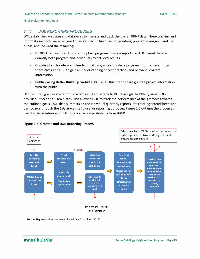
Savings and Economic Impacts of the Better Buildings Neighborhood Program DOE/EE-1203
Final Evaluation Volume 2
Better Buildings Neighborhood Program | Page 15
2.4.2. DOE REPORTING PROCESSES
DOE established websites and databases to manage and track the overall BBNP data. These tracking and
informational tools were designed to serve specific functions for grantees, program managers, and the
public, and included the following:
BBNIS. Grantees used this site to upload program progress reports, and DOE used the site to
quantify both program and individual project-level results.
Google Site. This site was intended to allow grantees to share program information amongst
themselves and DOE to gain an understanding of best practices and relevant program
information.
Public-Facing Better Buildings website. DOE used this site to share grantee project information
with the public.
DOE required grantees to report program results quarterly to DOE through the BBNIS, using DOE-
provided Excel or XML templates. This allowed DOE to track the performance of the grantees towards
the outlined goals. DOE then summarized the individual quarterly reports into tracking spreadsheets and
dashboards through the Salesforce site to use for reporting purposes. Figure 2-6 outlines the processes
used by the grantees and DOE to report accomplishments from BBNP.
Figure 2-6: Grantee and DOE Reporting Process
Source: Figure provided courtesy of Navigant Consulting (2013)

Savings and Economic Impacts of the Better Buildings Neighborhood Program DOE/EE-1203
Final Evaluation Volume 2
Better Buildings Neighborhood Program | Page 16
This reporting process created a system of checks and balances to address erroneous reporting issues.
However, as might be anticipated for a program of this scope and scale, issues occurred that impacted
the reporting of the accomplishments. Throughout the course of the BBNP, DOE and its consultants
targeted areas of concern and worked with the grantees to ensure better accuracy of their reporting.

Savings and Economic Impacts of the Better Buildings Neighborhood Program DOE/EE-1203
Final Evaluation Volume 2
Methodology | Page 17
3. METHODOLOGY
This chapter provides an overview of our evaluation methodology. It then provides additional discussion
of our sampling approach, our method of extrapolating our impact evaluation findings to develop a
verified savings estimate for the BBNP program overall, and additional metrics investigated. The chapter
concludes with a discussion of evaluation challenges.
Appendix B provides supplementary methodological detail.
3.1. OVERVIEW
The impact evaluation comprised two broad activities to determine gross verified savings:
M&V of a sample of grantees and projects
Billing regression analysis on projects from grantees with sufficient utility bill data
We combined the results from both M&V and billing regression analysis and extrapolated to the
population in order to determine the overall estimated energy savings for BBNP.
We used a sector based analysis (that is, residential, multifamily and commercial) that reviewed savings
associated with individual projects but not the individual measures making up each project.
We quantified impact metrics for the entire three-year BBNP grant cycle based on findings from
preliminary and final evaluations. The preliminary evaluation assessed a sample of projects reported
between Quarter 4 (Q4) 2010 and Quarter 2 (Q2) 2012 (inclusive).6 The final evaluation verified grantee
reported activities and quantified metrics for a sample of projects reported between Quarter 3 (Q3) of
2012 and Quarter 3 (Q3) of 2013. We conducted the preliminary research and analysis from January
2013 through May 2013; we conducted the final research and analysis from December 2013 to October
2014.
Although the preliminary and final evaluations use consistent and, for many of the assessment activities,
identical methodologies, our work plan for the final evaluation included refinements based on our
preliminary evaluation experiences. This chapter describes primarily the methodology we used for the
final evaluation activities, unless otherwise noted.
To conduct our analysis, we collected and analyzed data from the grantees and subgrantees as well as
program participants. Table 3-1 summarizes our data collection methods.
6 The preliminary evaluation had multiple goals: 1) to provide impact results mid-way through the BBNP program cycle; 2) to
refine the impact evaluation method for the final evaluation; 3) to support the process and market effect evaluation activities;
and 4) develop initial conclusions and recommendations that might be implemented by the grantees to foster an effective final
impact evaluation (Research Into Action, Evergreen Economics, Nexant, and NMR Group, 2013).
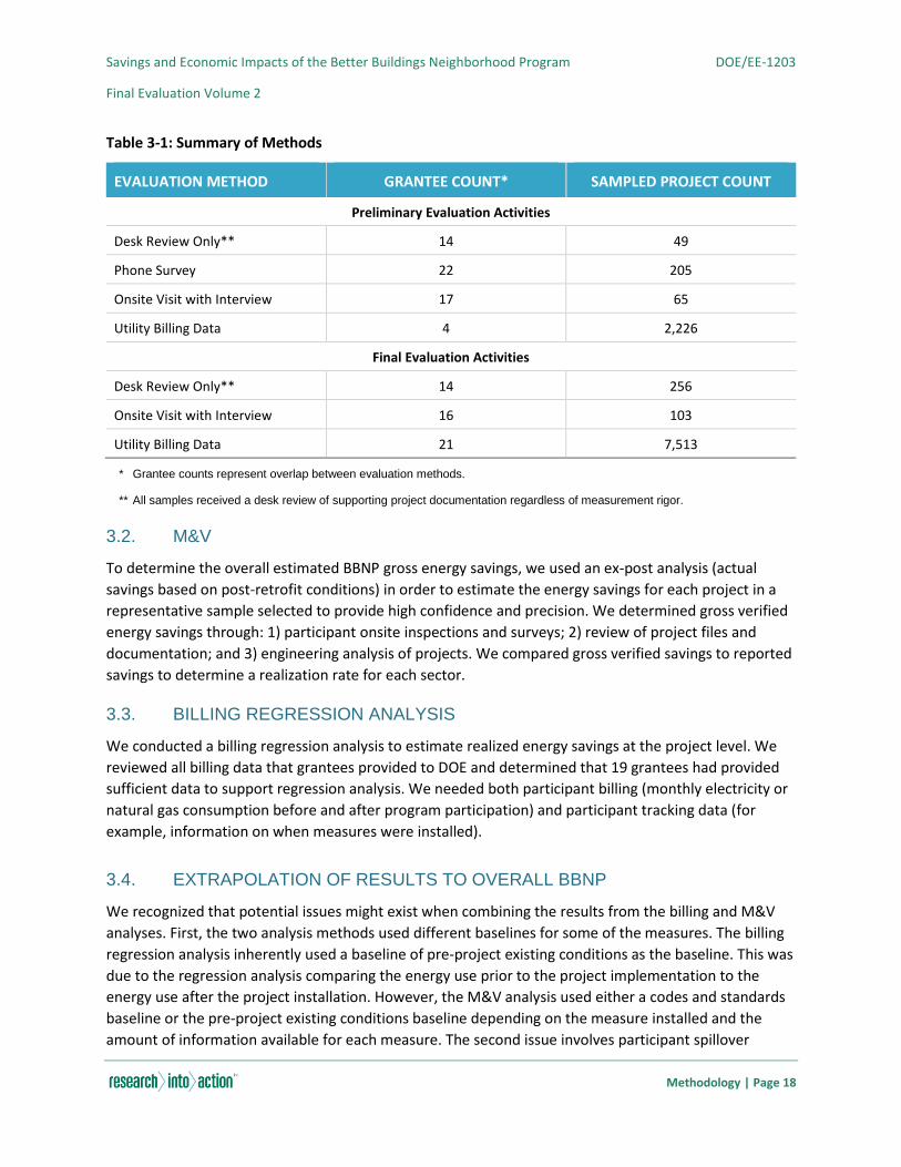
Savings and Economic Impacts of the Better Buildings Neighborhood Program DOE/EE-1203
Final Evaluation Volume 2
Methodology | Page 18
Table 3-1: Summary of Methods
EVALUATION METHOD GRANTEE COUNT* SAMPLED PROJECT COUNT
Preliminary Evaluation Activities
Desk Review Only** 14 49
Phone Survey 22 205
Onsite Visit with Interview 17 65
Utility Billing Data 4 2,226
Final Evaluation Activities
Desk Review Only** 14 256
Onsite Visit with Interview 16 103
Utility Billing Data 21 7,513
* Grantee counts represent overlap between evaluation methods.
** All samples received a desk review of supporting project documentation regardless of measurement rigor.
3.2. M&V
To determine the overall estimated BBNP gross energy savings, we used an ex-post analysis (actual
savings based on post-retrofit conditions) in order to estimate the energy savings for each project in a
representative sample selected to provide high confidence and precision. We determined gross verified
energy savings through: 1) participant onsite inspections and surveys; 2) review of project files and
documentation; and 3) engineering analysis of projects. We compared gross verified savings to reported
savings to determine a realization rate for each sector.
3.3. BILLING REGRESSION ANALYSIS
We conducted a billing regression analysis to estimate realized energy savings at the project level. We
reviewed all billing data that grantees provided to DOE and determined that 19 grantees had provided
sufficient data to support regression analysis. We needed both participant billing (monthly electricity or
natural gas consumption before and after program participation) and participant tracking data (for
example, information on when measures were installed).
3.4. EXTRAPOLATION OF RESULTS TO OVERALL BBNP
We recognized that potential issues might exist when combining the results from the billing and M&V
analyses. First, the two analysis methods used different baselines for some of the measures. The billing
regression analysis inherently used a baseline of pre-project existing conditions as the baseline. This was
due to the regression analysis comparing the energy use prior to the project implementation to the
energy use after the project installation. However, the M&V analysis used either a codes and standards
baseline or the pre-project existing conditions baseline depending on the measure installed and the
amount of information available for each measure. The second issue involves participant spillover
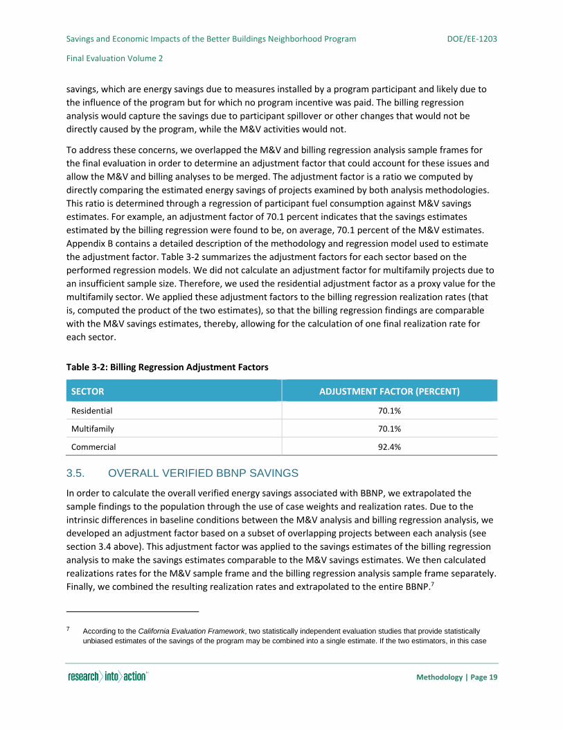
Savings and Economic Impacts of the Better Buildings Neighborhood Program DOE/EE-1203
Final Evaluation Volume 2
Methodology | Page 19
savings, which are energy savings due to measures installed by a program participant and likely due to
the influence of the program but for which no program incentive was paid. The billing regression
analysis would capture the savings due to participant spillover or other changes that would not be
directly caused by the program, while the M&V activities would not.
To address these concerns, we overlapped the M&V and billing regression analysis sample frames for
the final evaluation in order to determine an adjustment factor that could account for these issues and
allow the M&V and billing analyses to be merged. The adjustment factor is a ratio we computed by
directly comparing the estimated energy savings of projects examined by both analysis methodologies.
This ratio is determined through a regression of participant fuel consumption against M&V savings
estimates. For example, an adjustment factor of 70.1 percent indicates that the savings estimates
estimated by the billing regression were found to be, on average, 70.1 percent of the M&V estimates.
Appendix B contains a detailed description of the methodology and regression model used to estimate
the adjustment factor. Table 3-2 summarizes the adjustment factors for each sector based on the
performed regression models. We did not calculate an adjustment factor for multifamily projects due to
an insufficient sample size. Therefore, we used the residential adjustment factor as a proxy value for the
multifamily sector. We applied these adjustment factors to the billing regression realization rates (that
is, computed the product of the two estimates), so that the billing regression findings are comparable
with the M&V savings estimates, thereby, allowing for the calculation of one final realization rate for
each sector.
Table 3-2: Billing Regression Adjustment Factors
SECTOR ADJUSTMENT FACTOR (PERCENT)
Residential 70.1%
Multifamily 70.1%
Commercial 92.4%
3.5. OVERALL VERIFIED BBNP SAVINGS
In order to calculate the overall verified energy savings associated with BBNP, we extrapolated the
sample findings to the population through the use of case weights and realization rates. Due to the
intrinsic differences in baseline conditions between the M&V analysis and billing regression analysis, we
developed an adjustment factor based on a subset of overlapping projects between each analysis (see
section 3.4 above). This adjustment factor was applied to the savings estimates of the billing regression
analysis to make the savings estimates comparable to the M&V savings estimates. We then calculated
realizations rates for the M&V sample frame and the billing regression analysis sample frame separately.
Finally, we combined the resulting realization rates and extrapolated to the entire BBNP.7
7 According to the California Evaluation Framework, two statistically independent evaluation studies that provide statistically
unbiased estimates of the savings of the program may be combined into a single estimate. If the two estimators, in this case

Savings and Economic Impacts of the Better Buildings Neighborhood Program DOE/EE-1203
Final Evaluation Volume 2
Methodology | Page 20
We combined the M&V realization rates for both the preliminary and final evaluations in order to
determine an M&V realization rate representative of the entire evaluation timeframe. We calculated the
combined M&V realization rate through a weighted average of the realization rates based on the total
ex ante savings of all the grantees within each respective sampling frame. We could not calculate a
weighted realization rate for the multifamily sector as no realization rate was calculated for this sector
during the preliminary evaluation.
We also used the billing regression results to develop realization rates for the all sectors. We calculated
these realization rates for each grantee that provided billing data and where robust billing regression
models could be estimated. To develop a realization rate for the billing regression analysis sample, we
calculated a weighted average of the grantee-level realization rates that were estimated using the billing
regression, with ex ante savings used as the weights.
BBNP savings reported by DOE for the sample was adjusted to reflect the findings of the M&V and billing
regression analysis activities.
We calculated the overall sector realization rate by taking a weighted average of the realization rates
calculated for the M&V and the billing regression analyses. The team weighted these realization rates
based on the total ex ante savings of all the grantees within each respective sampling frame. Once we
determined the weighted average realization rate, we applied this value to the overall reported savings
for the sector population to calculate a gross verified savings. We then calculated net verified savings for
each sector by applying the NTG ratio to the sector level gross verified savings.
3.6. ADDITIONAL OVERALL BBNP METRICS
3.6.1. GREENHOUSE GAS EMISSION SAVINGS
We calculated and reported carbon dioxide (CO2e) equivalent reductions based on verified net source
savings for each year over the effective useful lifetime of the projects evaluated. We expressed the
emission factor as mass per unit of energy (metric tons of CO2e per MMBtu), which represents the
characteristics of the emission sources displaced by reduced generation from conventional sources of
electricity or reduced consumption of natural gas.
We sourced emission factors for electricity from the U.S. Environmental Protection Agency’s (EPA)
eGrid8 dataset. Emission factors for average U.S. annual non-baseload output for carbon dioxide,
methane, and nitrous oxide were used to calculate a CO2e emissions factor. We used non-baseload
output to calculate the emissions factor as energy efficiency programs are generally assumed not to
the realization rates from the M&V analysis and the billing regression analysis, are both unbiased estimators of a given
parameter, then any weighted average of the two estimators also is an unbiased estimator. The error bound of the result is the
square root of the reciprocal of the sum of the weights (TecMarket Works, 2004).
8 Emissions & Generation Resource Integrated Database, 9th edition Version 1.0 Year 2010 GHG Annual Output Emission
Rates. The national-level emissions factor was used to convert total net electricity savings to avoided greenhouse gas (GHG)
emissions.
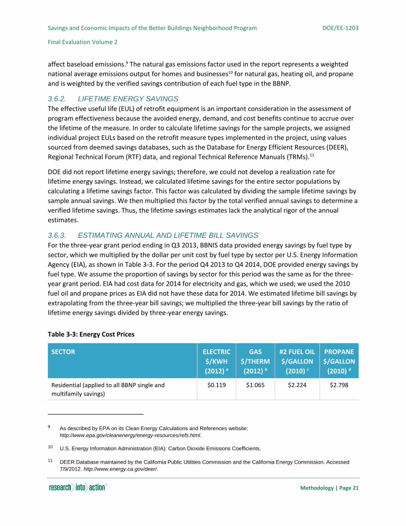
Savings and Economic Impacts of the Better Buildings Neighborhood Program DOE/EE-1203
Final Evaluation Volume 2
Methodology | Page 21
affect baseload emissions.9 The natural gas emissions factor used in the report represents a weighted
national average emissions output for homes and businesses10 for natural gas, heating oil, and propane
and is weighted by the verified savings contribution of each fuel type in the BBNP.
3.6.2. LIFETIME ENERGY SAVINGS
The effective useful life (EUL) of retrofit equipment is an important consideration in the assessment of
program effectiveness because the avoided energy, demand, and cost benefits continue to accrue over
the lifetime of the measure. In order to calculate lifetime savings for the sample projects, we assigned
individual project EULs based on the retrofit measure types implemented in the project, using values
sourced from deemed savings databases, such as the Database for Energy Efficient Resources (DEER),
Regional Technical Forum (RTF) data, and regional Technical Reference Manuals (TRMs).11
DOE did not report lifetime energy savings; therefore, we could not develop a realization rate for
lifetime energy savings. Instead, we calculated lifetime savings for the entire sector populations by
calculating a lifetime savings factor. This factor was calculated by dividing the sample lifetime savings by
sample annual savings. We then multiplied this factor by the total verified annual savings to determine a
verified lifetime savings. Thus, the lifetime savings estimates lack the analytical rigor of the annual
estimates.
3.6.3. ESTIMATING ANNUAL AND LIFETIME BILL SAVINGS
For the three-year grant period ending in Q3 2013, BBNIS data provided energy savings by fuel type by
sector, which we multiplied by the dollar per unit cost by fuel type by sector per U.S. Energy Information
Agency (EIA), as shown in Table 3-3. For the period Q4 2013 to Q4 2014, DOE provided energy savings by
fuel type. We assume the proportion of savings by sector for this period was the same as for the three-
year grant period. EIA had cost data for 2014 for electricity and gas, which we used; we used the 2010
fuel oil and propane prices as EIA did not have these data for 2014. We estimated lifetime bill savings by
extrapolating from the three-year bill savings; we multiplied the three-year bill savings by the ratio of
lifetime energy savings divided by three-year energy savings.
Table 3-3: Energy Cost Prices
SECTOR ELECTRIC
$/KWH
(2012) a
GAS
$/THERM
(2012) b
#2 FUEL OIL
$/GALLON
(2010) c
PROPANE
$/GALLON
(2010) d
Residential (applied to all BBNP single and
multifamily savings)
$0.119 $1.065 $2.224 $2.798
9 As described by EPA on its Clean Energy Calculations and References website:
http://www.epa.gov/cleanenergy/energy-resources/refs.html.
10 U.S. Energy Information Administration (EIA): Carbon Dioxide Emissions Coefficients.
11 DEER Database maintained by the California Public Utilities Commission and the California Energy Commission. Accessed
7/9/2012. http://www.energy.ca.gov/deer/.
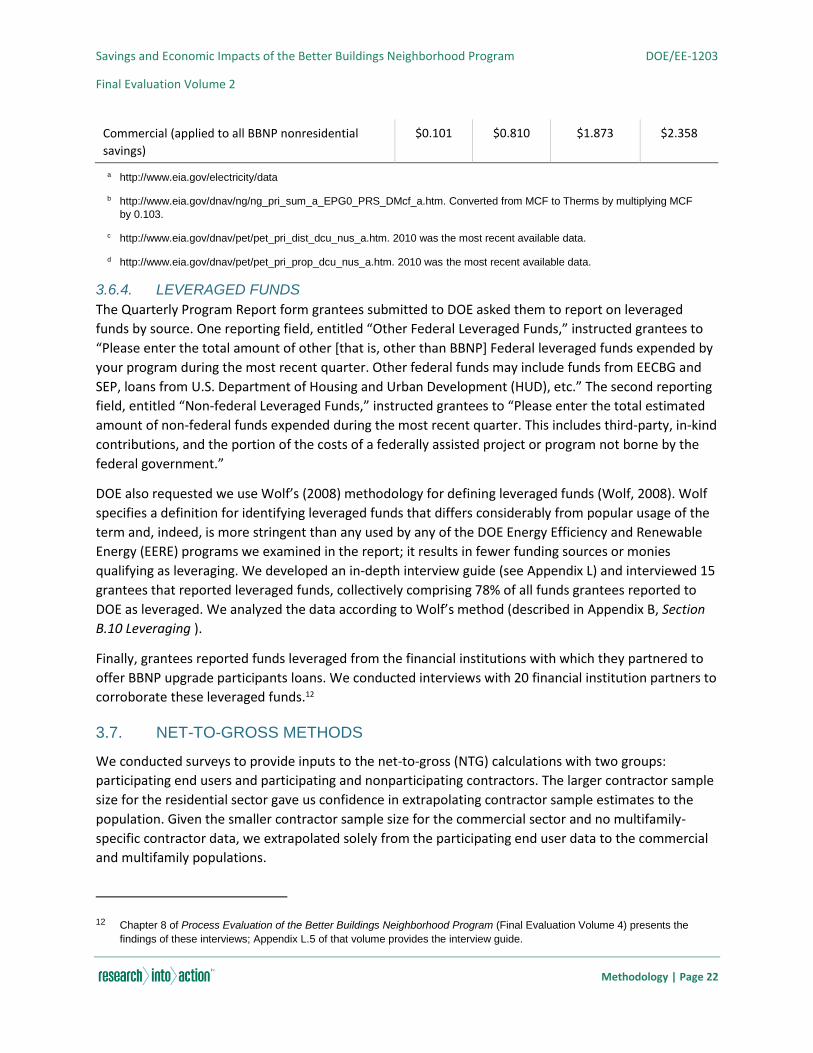
Savings and Economic Impacts of the Better Buildings Neighborhood Program DOE/EE-1203
Final Evaluation Volume 2
Methodology | Page 22
Commercial (applied to all BBNP nonresidential
savings)
$0.101 $0.810 $1.873 $2.358
a http://www.eia.gov/electricity/data
b http://www.eia.gov/dnav/ng/ng_pri_sum_a_EPG0_PRS_DMcf_a.htm. Converted from MCF to Therms by multiplying MCF
by 0.103.
c http://www.eia.gov/dnav/pet/pet_pri_dist_dcu_nus_a.htm. 2010 was the most recent available data.
d http://www.eia.gov/dnav/pet/pet_pri_prop_dcu_nus_a.htm. 2010 was the most recent available data.
3.6.4. LEVERAGED FUNDS
The Quarterly Program Report form grantees submitted to DOE asked them to report on leveraged
funds by source. One reporting field, entitled “Other Federal Leveraged Funds,” instructed grantees to
“Please enter the total amount of other [that is, other than BBNP] Federal leveraged funds expended by
your program during the most recent quarter. Other federal funds may include funds from EECBG and
SEP, loans from U.S. Department of Housing and Urban Development (HUD), etc.” The second reporting
field, entitled “Non-federal Leveraged Funds,” instructed grantees to “Please enter the total estimated
amount of non-federal funds expended during the most recent quarter. This includes third-party, in-kind
contributions, and the portion of the costs of a federally assisted project or program not borne by the
federal government.”
DOE also requested we use Wolf’s (2008) methodology for defining leveraged funds (Wolf, 2008). Wolf
specifies a definition for identifying leveraged funds that differs considerably from popular usage of the
term and, indeed, is more stringent than any used by any of the DOE Energy Efficiency and Renewable
Energy (EERE) programs we examined in the report; it results in fewer funding sources or monies
qualifying as leveraging. We developed an in-depth interview guide (see Appendix L) and interviewed 15
grantees that reported leveraged funds, collectively comprising 78% of all funds grantees reported to
DOE as leveraged. We analyzed the data according to Wolf’s method (described in Appendix B, Section
B.10 Leveraging ).
Finally, grantees reported funds leveraged from the financial institutions with which they partnered to
offer BBNP upgrade participants loans. We conducted interviews with 20 financial institution partners to
corroborate these leveraged funds.12
3.7. NET-TO-GROSS METHODS
We conducted surveys to provide inputs to the net-to-gross (NTG) calculations with two groups:
participating end users and participating and nonparticipating contractors. The larger contractor sample
size for the residential sector gave us confidence in extrapolating contractor sample estimates to the
population. Given the smaller contractor sample size for the commercial sector and no multifamily-
specific contractor data, we extrapolated solely from the participating end user data to the commercial
and multifamily populations.
12 Chapter 8 of Process Evaluation of the Better Buildings Neighborhood Program (Final Evaluation Volume 4) presents the
findings of these interviews; Appendix L.5 of that volume provides the interview guide.
Savings and Economic Impacts of the Better Buildings Neighborhood Program DOE/EE-1203
Final Evaluation Volume 2
Methodology | Page 23
Residential: The final NTG estimate for the residential sector is based on both end user- and contractor-
derived NTG estimates. Participating end user free-ridership informs the lower bound NTG estimates
(that is, NTG with free-ridership), and contractor-derived estimates of free-ridership and spillover inform
the upper bound NTG estimates (that is, NTG with free-ridership and spillover). The final residential NTG
value is the mid-point between the lower and upper bounds (that is, the end user- and contractor-
derived NTG estimates).
Commercial and Multifamily: The final NTG estimates for the commercial and multifamily sector are
derived solely from participating end user free-ridership. While there are some indications of spillover
from the commercial grantees, the sample size of surveyed contractors was too small to develop a
reliable estimate.
See Appendix B and Market Effects of the Better Buildings Neighborhood Program (Final Evaluation
Volume 5) for additional details on the NTG methodology.
3.7.1. LOWER BOUND NET-TO-GROSS RATIO ESTIMATES DERIVED FROM
PARTICIPATING END USERS
Sampled commercial end users were those that completed an onsite verification survey as part of the
M&V activities for the final evaluation; the onsite verification survey included the NTG questions. We
sampled multifamily end users from a desk review and conducted the NTG survey over the phone.
Sampled residential end users were those that completed an online survey that included process and
NTG questions. Our survey questions sought information relating both to program influence (free-
ridership) and spillover; however, we are able to provide numeric estimates of free-ridership only. (Our
study methodology did not include estimation of energy savings associated with respondents’ reported
spillover activity, nor with verifying the spillover.) We compiled the free-ridership results for each
project from two components, what the participant would likely have done in the absence of the
program and the influence the participant states that the program had on the upgrade actions taken.
For commercial and multifamily sectors (which were based on the M&V sample), we rolled up the per-
project results to the stratum level within each sector. We multiplied the stratum-average free-ridership
score by the stratum verified savings and summed the resulting stratum-net-savings to obtain a sector
net savings. We calculated sector NTG as the ratio of the sector-net-savings divided by the sector-
verified-savings. We calculated the residential lower bound NTG using an analogous approach, but used
grantee-stratum case weights developed by multiplying the ratio of a grantee’s total project count to
total BBNP project count by the ratio of respondents in the grantee’s stratum to total survey
respondents.
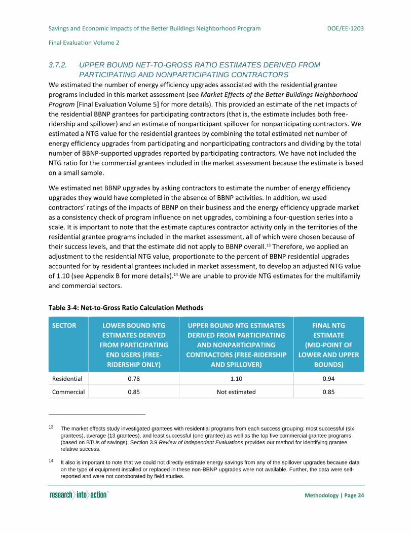
Savings and Economic Impacts of the Better Buildings Neighborhood Program DOE/EE-1203
Final Evaluation Volume 2
Methodology | Page 24
3.7.2. UPPER BOUND NET-TO-GROSS RATIO ESTIMATES DERIVED FROM
PARTICIPATING AND NONPARTICIPATING CONTRACTORS
We estimated the number of energy efficiency upgrades associated with the residential grantee
programs included in this market assessment (see Market Effects of the Better Buildings Neighborhood
Program [Final Evaluation Volume 5] for more details). This provided an estimate of the net impacts of
the residential BBNP grantees for participating contractors (that is, the estimate includes both free-
ridership and spillover) and an estimate of nonparticipant spillover for nonparticipating contractors. We
estimated a NTG value for the residential grantees by combining the total estimated net number of
energy efficiency upgrades from participating and nonparticipating contractors and dividing by the total
number of BBNP-supported upgrades reported by participating contractors. We have not included the
NTG ratio for the commercial grantees included in the market assessment because the estimate is based
on a small sample.
We estimated net BBNP upgrades by asking contractors to estimate the number of energy efficiency
upgrades they would have completed in the absence of BBNP activities. In addition, we used
contractors’ ratings of the impacts of BBNP on their business and the energy efficiency upgrade market
as a consistency check of program influence on net upgrades, combining a four-question series into a
scale. It is important to note that the estimate captures contractor activity only in the territories of the
residential grantee programs included in the market assessment, all of which were chosen because of
their success levels, and that the estimate did not apply to BBNP overall.13 Therefore, we applied an
adjustment to the residential NTG value, proportionate to the percent of BBNP residential upgrades
accounted for by residential grantees included in market assessment, to develop an adjusted NTG value
of 1.10 (see Appendix B for more details).14 We are unable to provide NTG estimates for the multifamily
and commercial sectors.
Table 3-4: Net-to-Gross Ratio Calculation Methods
SECTOR LOWER BOUND NTG
ESTIMATES DERIVED
FROM PARTICIPATING
END USERS (FREE-
RIDERSHIP ONLY)
UPPER BOUND NTG ESTIMATES
DERIVED FROM PARTICIPATING
AND NONPARTICIPATING
CONTRACTORS (FREE-RIDERSHIP
AND SPILLOVER)
FINAL NTG
ESTIMATE
(MID-POINT OF
LOWER AND UPPER
BOUNDS)
Residential 0.78 1.10 0.94
Commercial 0.85 Not estimated 0.85
13 The market effects study investigated grantees with residential programs from each success grouping: most successful (six
grantees), average (13 grantees), and least successful (one grantee) as well as the top five commercial grantee programs
(based on BTUs of savings). Section 3.9 Review of Independent Evaluations provides our method for identifying grantee
relative success.
14 It also is important to note that we could not directly estimate energy savings from any of the spillover upgrades because data
on the type of equipment installed or replaced in these non-BBNP upgrades were not available. Further, the data were self-
reported and were not corroborated by field studies.
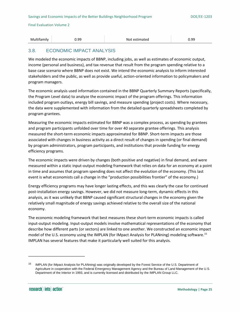
Savings and Economic Impacts of the Better Buildings Neighborhood Program DOE/EE-1203
Final Evaluation Volume 2
Methodology | Page 25
Multifamily 0.99 Not estimated 0.99
3.8. ECONOMIC IMPACT ANALYSIS
We modeled the economic impacts of BBNP, including jobs, as well as estimates of economic output,
income (personal and business), and tax revenue that result from the program spending relative to a
base case scenario where BBNP does not exist. We intend the economic analysis to inform interested
stakeholders and the public, as well as provide useful, action-oriented information to policymakers and
program managers.
The economic analysis used information contained in the BBNP Quarterly Summary Reports (specifically,
the Program Level data) to analyze the economic impact of the program offerings. This information
included program outlays, energy bill savings, and measure spending (project costs). Where necessary,
the data were supplemented with information from the detailed quarterly spreadsheets completed by
program grantees.
Measuring the economic impacts estimated for BBNP was a complex process, as spending by grantees
and program participants unfolded over time for over 40 separate grantee offerings. This analysis
measured the short-term economic impacts approximated for BBNP. Short-term impacts are those
associated with changes in business activity as a direct result of changes in spending (or final demand)
by program administrators, program participants, and institutions that provide funding for energy
efficiency programs.
The economic impacts were driven by changes (both positive and negative) in final demand, and were
measured within a static input-output modeling framework that relies on data for an economy at a point
in time and assumes that program spending does not affect the evolution of the economy. (This last
event is what economists call a change in the “production possibilities frontier” of the economy.)
Energy efficiency programs may have longer lasting effects, and this was clearly the case for continued
post-installation energy savings. However, we did not measure long-term, dynamic effects in this
analysis, as it was unlikely that BBNP caused significant structural changes in the economy given the
relatively small magnitude of energy savings achieved relative to the overall size of the national
economy.
The economic modeling framework that best measures these short-term economic impacts is called
input-output modeling. Input-output models involve mathematical representations of the economy that
describe how different parts (or sectors) are linked to one another. We constructed an economic impact
model of the U.S. economy using the IMPLAN (for IMpact Analysis for PLANning) modeling software.15
IMPLAN has several features that make it particularly well suited for this analysis.
15 IMPLAN (for IMpact Analysis for PLANning) was originally developed by the Forest Service of the U.S. Department of
Agriculture in cooperation with the Federal Emergency Management Agency and the Bureau of Land Management of the U.S.
Department of the Interior in 1993, and is currently licensed and distributed by the IMPLAN Group LLC.
Savings and Economic Impacts of the Better Buildings Neighborhood Program DOE/EE-1203
Final Evaluation Volume 2
Methodology | Page 26
Input-output analysis employs specific terminology to identify the different types of economic impacts.
BBNP affected the economy directly through the purchase of goods and services. Under our program-
centric approach, these direct impacts included jobs16 and income for grantee staff that administer and
manage energy efficiency programs, contractors who provide audit and retrofit services, and energy
efficiency equipment manufacturers. Direct effects also included changes in spending or output
resultant to the energy savings for participating households and businesses.
These direct changes in economic activity will, in turn, indirectly generate purchases of intermediate
goods and services from other related sectors of the economy. Because these indirect purchases
represent interactions among businesses, they are often referred to as “supply-chain” impacts.
In addition, the direct and indirect increases in employment increase income, which expands consumer
spending and enhances overall economy purchasing power, thereby inducing further consumption- and
investment-driven stimulus. These induced effects are often referred to as “consumption-driven”
impacts. In this report, the indirect and induced impacts are grouped together and reported as
“secondary” impacts.
The model includes the following elements: 1) It captures upgrade project costs – that is, both the
incented and unincented portions of project costs are captured in BBNP-related spending; 2) It describes
net verified project energy savings; 3) It reduces activity in the generation sector commensurate with
project energy savings; and 4) It does not include leveraged funds, such as funds leveraged from
financial institutions, on the assumption that these amounts are largely reflected in upgrade project
costs.
Increasing the total inputs to compensate for leveraged resources would result in double counting the
impacts derived from these moneys and therefore overestimate the economic impacts of BBNP
3.9. REVIEW OF INDEPENDENT EVALUATIONS
We identified 20 grantee-level program impact evaluations conducted by independent (also known as
third party) evaluators. However, the majority of these documents were process evaluations, marketing
evaluations, informational brochures, or memos regarding the program. We benchmarked six third
party impact evaluations and identified one for inclusion in our evaluation of the BBNP.
16 The IMPLAN modeling software measures jobs as the annual average of monthly jobs in each industry (this is the same
definition used by Quarterly Census of Employment and Wages [QCEW], U.S. Bureau of Labor Statistics [BLS], and U.S.
Bureau of Economic Analysis [BEA] nationally). Thus, one job is equivalent to one person being employed for the duration of
one year, two people being employed for half a year each, three people being employed for a third of a year each, etc.
Furthermore, IMPLAN jobs include full-time, part-time, and temporary positions. For reporting purposes, all IMPLAN job
estimates in this report have been converted to full-time equivalents (2,080 hours in a standard year) using the sector-level
conversion spreadsheet available on IMPLAN Group’s website. For more information please see:
https://implan.com/index.php?view=document&alias=206-convert-implan-employment-to-fte-and-wage-and-salary-data-to-
employee-compensation&category_slug=version-three-files&layout=default&option=com_docman&Itemid=1370

Savings and Economic Impacts of the Better Buildings Neighborhood Program DOE/EE-1203
Final Evaluation Volume 2
Methodology | Page 27
3.10. ASSESSING GRANTEE SUCCESS
A primary goal of our evaluation was to identify factors that drove or inhibited success among grantees’
and subgrantees’ residential upgrade programs. To support the statistical investigation of effective
approaches to delivering residential upgrade programs, Drivers of Success in the Better Buildings
Neighborhood Program – Statistical Process Evaluation (Final Evaluation Volume 3) identified 12 diverse
quantitative performance indicators, such as average MMBtu savings per project, program cost per
upgrade, and progress toward upgrade goal. We then clustered grantees into groups based on their
performance on the 12 metrics using grantee-reported residential activity data (Q4 2010 to Q3 2013).
The analyses yielded three groups of grantees whose average performance on the 12 metrics were
consistent with an interpretation of a most successful group, an average group, and a least successful
group.
We emphasize here that the Volume 3 analysis used the grantee success clustering only to identify
programmatic elements associated with stronger performance relative to other grantees, a research
objective important to the DOE BBNP team. As we note elsewhere, grantee success during the three-
year evaluation period was associated with the length of time programs took to reach optimal
functioning; the most successful grantees reached the optimum point in their programs six months
sooner than less successful grantees. However, we did not find that grantee success was driven by prior
whole home program experience. Nonetheless, were the grantee programs to continue for ten years,
we would expect program achievements to be higher in later years than in the initial years as grantees
gained experience in their markets and adjusted their programs accordingly.
As we report in Volume 3, using both data that grantees reported to DOE in partial fulfillment of their
grant requirements and data collected by our team, we conducted a series of statistical analyses to
develop a quantitative definition of grantee success that corresponds to BBNP’s multiple program
objectives and to identify program features and characteristics that predict success.
Due to the greater availability of data for residential programs compared with multifamily and
commercial programs, the Volume 3 success analysis focused exclusively on residential programs.
Further, if a grant recipient had subgrantees that ran separate and distinct programs in mutually
exclusive regions, we collected and analyzed data from each individual subgrantee to capture the full
diversity of program models, outcomes, and market characteristics. A total of 54 grantees and
subgrantees with residential programs were included in these analyses.
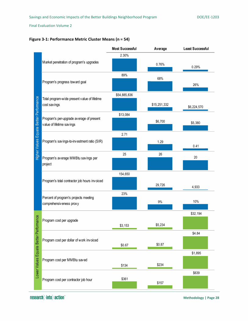
Savings and Economic Impacts of the Better Buildings Neighborhood Program DOE/EE-1203
Final Evaluation Volume 2
Methodology | Page 28
Figure 3-1: Performance Metric Cluster Means (n = 54)
Most Successful Average Least Successful
2.30%
89%
$54,885,836
$13,084
2.71
25 26
154,650
23%
$32,194
$4.84
$1,895
$639
Program's sav ings-to-investment ratio (SIR)
Lo
we
r V
alu
es
Eq
ua
te B
ett
er
Pe
rfo
rma
nce
Program cost per upgrade
Program cost per dollar of work invoiced
Program cost per MMBtu saved
Program cost per contractor job hour
Program's average MMBtu sav ings per
project
Program's total contractor job hours invoiced
Percent of program's projects meeting
comprehensiveness proxy
Hig
he
r V
alu
es
Eq
ua
te B
ett
er
Pe
rfo
rma
nce
Market penetration of program's upgrades
Program's progress toward goal
Total program-wide present value of lifetime
cost sav ings
Program's per-upgrade average of present
value of lifetime savings
0.76%0.29%
26%
68%
$15,251,332$6,224,570
$6,700 $5,380
20
29,7264,933
9% 10%
$5,234$3,153
$0.67 $0.87
$134 $234
$157$361
0.41
1.29

Savings and Economic Impacts of the Better Buildings Neighborhood Program DOE/EE-1203
Final Evaluation Volume 2
Methodology | Page 29
First, we defined a broad range of potential measurements of program success based on theory and
industry knowledge. From this list, we identified 12 quantitative performance metrics for which there
were adequate data. We then conducted latent profile analysis (LPA) to cluster programs into groups
that exhibited similar performance on the 12 performance metrics. LPA is an exploratory analytical
technique, and our analyses sought to identify groups, or clusters, of grantees that differed meaningfully
in their performance on 12 metrics of program success.
The LPA yielded three groups, and their average group values on the 12 performance metrics were
consistent with an interpretation of a most successful cluster (n = 12), an average cluster (n = 35), and a
least successful cluster
(n = 7). The most successful cluster generally performed best on each of the metrics, the least successful
cluster generally performed worst on the metrics, and the average cluster demonstrated middling
values on the performance metrics. Thus, the LPA revealed clusters of grantees that were more or less
successful relative to one another. Figure 3-1, a copy of Figure 3-1 in Volume 3, demonstrates these
tiered levels of grantee success by displaying the average cluster means for each of the 12 performance
metrics.
Next, we identified grantee and program characteristics that may predict program success and compiled
the corresponding data. This dataset also included exogenous variables that we deemed as critical
control variables, such as weather metrics, average energy price, median income, and other variables
that may affect energy use, savings, and participation rates. We used bivariate logistic regression models
to explore whether any of the proposed predictor variables predicted membership in either the least
successful cluster or the most successful cluster, respectively. We report the bivariate findings in
companion volume Process Evaluation of the Better Buildings Neighborhood Program (Final Evaluation
Volume 4). Next, we ran multivariate regression models for each dependent variable (membership in
the least successful cluster versus other and membership in the most successful cluster versus other)
using the independent variables identified as meaningful predictors in the aforementioned bivariate
models. We report the multivariate findings in Volume 3. Findings relevant to the savings and economic
impacts are discussed throughout this volume. For additional information on the methods used to
identify the grantee success clusters, see Volume 3.
3.11. SAMPLING
We selected unique sample frames for the M&V and the billing regression analysis assessments, as
described in Table 3-5. As noted, the billing regression sample was dictated by the availability of
sufficient grantee billing data required to conduct the billing regression analysis.
Table 3-5: Grantee Sample Frame by Evaluation Activity
EVALUATION ACTIVITY NUMBER OF
GRANTEES
IN SAMPLE FRAME
NUMBER OF PROJECTS
IN SAMPLE FRAME
REPORTED ENERGY
SAVINGS IN SAMPLE
FRAME (MMBtus)
M&V 30 41,541 3,026,023
Billing regression analysis 19 16,294 1,237,045
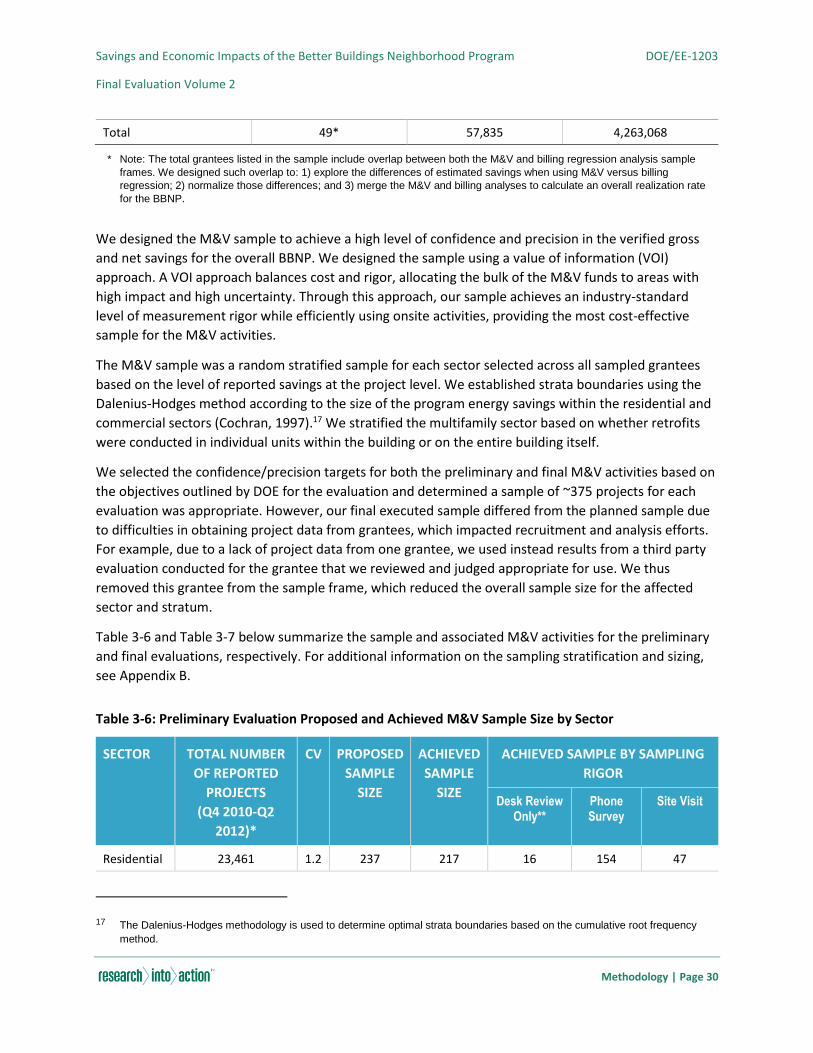
Savings and Economic Impacts of the Better Buildings Neighborhood Program DOE/EE-1203
Final Evaluation Volume 2
Methodology | Page 30
Total 49* 57,835 4,263,068
* Note: The total grantees listed in the sample include overlap between both the M&V and billing regression analysis sample
frames. We designed such overlap to: 1) explore the differences of estimated savings when using M&V versus billing
regression; 2) normalize those differences; and 3) merge the M&V and billing analyses to calculate an overall realization rate
for the BBNP.
We designed the M&V sample to achieve a high level of confidence and precision in the verified gross
and net savings for the overall BBNP. We designed the sample using a value of information (VOI)
approach. A VOI approach balances cost and rigor, allocating the bulk of the M&V funds to areas with
high impact and high uncertainty. Through this approach, our sample achieves an industry-standard
level of measurement rigor while efficiently using onsite activities, providing the most cost-effective
sample for the M&V activities.
The M&V sample was a random stratified sample for each sector selected across all sampled grantees
based on the level of reported savings at the project level. We established strata boundaries using the
Dalenius-Hodges method according to the size of the program energy savings within the residential and
commercial sectors (Cochran, 1997).17 We stratified the multifamily sector based on whether retrofits
were conducted in individual units within the building or on the entire building itself.
We selected the confidence/precision targets for both the preliminary and final M&V activities based on
the objectives outlined by DOE for the evaluation and determined a sample of ~375 projects for each
evaluation was appropriate. However, our final executed sample differed from the planned sample due
to difficulties in obtaining project data from grantees, which impacted recruitment and analysis efforts.
For example, due to a lack of project data from one grantee, we used instead results from a third party
evaluation conducted for the grantee that we reviewed and judged appropriate for use. We thus
removed this grantee from the sample frame, which reduced the overall sample size for the affected
sector and stratum.
Table 3-6 and Table 3-7 below summarize the sample and associated M&V activities for the preliminary
and final evaluations, respectively. For additional information on the sampling stratification and sizing,
see Appendix B.
Table 3-6: Preliminary Evaluation Proposed and Achieved M&V Sample Size by Sector
SECTOR TOTAL NUMBER
OF REPORTED
PROJECTS
(Q4 2010-Q2
2012)*
CV PROPOSED
SAMPLE
SIZE
ACHIEVED
SAMPLE
SIZE
ACHIEVED SAMPLE BY SAMPLING
RIGOR
Desk Review Only**
Phone Survey
Site Visit
Residential 23,461 1.2 237 217 16 154 47
17 The Dalenius-Hodges methodology is used to determine optimal strata boundaries based on the cumulative root frequency
method.
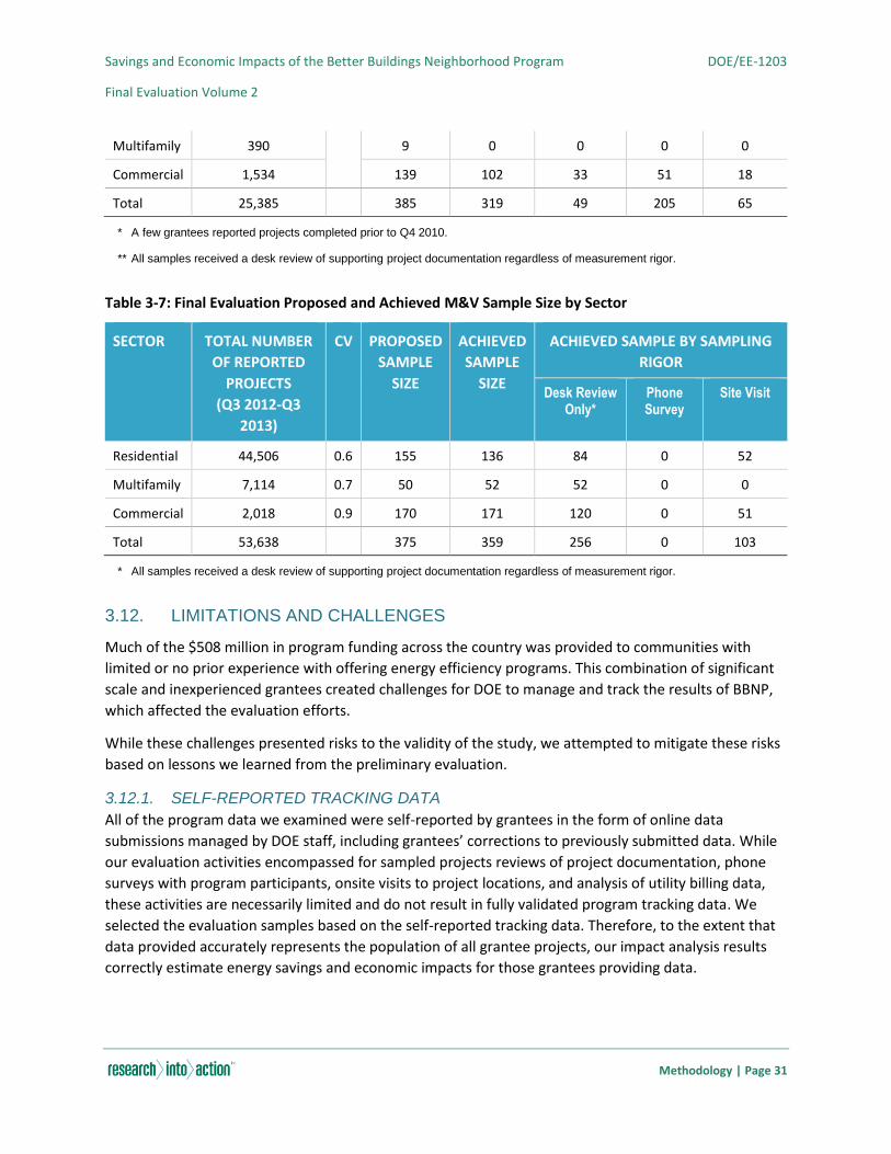
Savings and Economic Impacts of the Better Buildings Neighborhood Program DOE/EE-1203
Final Evaluation Volume 2
Methodology | Page 31
Multifamily 390 9 0 0 0 0
Commercial 1,534 139 102 33 51 18
Total 25,385 385 319 49 205 65
* A few grantees reported projects completed prior to Q4 2010.
** All samples received a desk review of supporting project documentation regardless of measurement rigor.
Table 3-7: Final Evaluation Proposed and Achieved M&V Sample Size by Sector
SECTOR TOTAL NUMBER
OF REPORTED
PROJECTS
(Q3 2012-Q3
2013)
CV PROPOSED
SAMPLE
SIZE
ACHIEVED
SAMPLE
SIZE
ACHIEVED SAMPLE BY SAMPLING
RIGOR
Desk Review Only*
Phone Survey
Site Visit
Residential 44,506 0.6 155 136 84 0 52
Multifamily 7,114 0.7 50 52 52 0 0
Commercial 2,018 0.9 170 171 120 0 51
Total 53,638 375 359 256 0 103
* All samples received a desk review of supporting project documentation regardless of measurement rigor.
3.12. LIMITATIONS AND CHALLENGES
Much of the $508 million in program funding across the country was provided to communities with
limited or no prior experience with offering energy efficiency programs. This combination of significant
scale and inexperienced grantees created challenges for DOE to manage and track the results of BBNP,
which affected the evaluation efforts.
While these challenges presented risks to the validity of the study, we attempted to mitigate these risks
based on lessons we learned from the preliminary evaluation.
3.12.1. SELF-REPORTED TRACKING DATA
All of the program data we examined were self-reported by grantees in the form of online data
submissions managed by DOE staff, including grantees’ corrections to previously submitted data. While
our evaluation activities encompassed for sampled projects reviews of project documentation, phone
surveys with program participants, onsite visits to project locations, and analysis of utility billing data,
these activities are necessarily limited and do not result in fully validated program tracking data. We
selected the evaluation samples based on the self-reported tracking data. Therefore, to the extent that
data provided accurately represents the population of all grantee projects, our impact analysis results
correctly estimate energy savings and economic impacts for those grantees providing data.

Savings and Economic Impacts of the Better Buildings Neighborhood Program DOE/EE-1203
Final Evaluation Volume 2
Methodology | Page 32
3.12.2. DIFFICULTY INTERPRETING GRANTEE DATA
The grantees were responsible for submitting metrics associated with project impacts and program
operation on a quarterly basis to DOE, yet DOE did not specify or restrict data tracking methods that the
grantees used to generate the data they uploaded to DOE’s database. The variation in grantee data
tracking and quality created a number of challenges to our understanding and interpretation of the
data. The four main issues that came out of this challenge included:
1. Quantification of Savings. In order to calculate the estimated energy savings reported to DOE,
grantees use a deemed approach, modeled approach, or a combination of both. The deemed
approach involved the use of predetermined energy savings values for measures implemented
for each project. The modeled approach involved the use of energy models that are built
specifically to the project parameters (that is, building type, sq. ft., energy using systems,
weather, etc.) in order to determine an energy savings estimate. However, the inputs that were
used in these calculations were often not available to us. Consequently, we often had no insight
into the methodology for the calculation of savings and, thus, could not easily identify potential
reasons for discrepancies between verified savings and reported savings.
2. Grantee Reporting. Grantees had two options for reporting savings to DOE. These two reporting
options resulted in DOE receiving very different levels of information. In addition, the level of
detail that grantees provided on DOE reporting forms varied substantially. In response, DOE
implemented a separate methodology to capture the required information. Section 3.3 provides
further explanation.
3. Project Tracking. All of the grantees tracked project information differently and maintained
varying levels of information regarding project implementation activities. Some maintained only
tracking databases with a limited level of information, while others kept detailed project records
complete with rebate applications or invoices. Therefore, we faced challenges when verifying
measure specific details at some of the project sites.
4. Billing Data. As part of the grant specifications, grantees were tasked with the collection of
billing data for all completed projects. However, this proved difficult for many of the grantees
due to the challenges associated with obtaining utility bills from the utility provider. Thus, only
half of all grantees were able to collect utility bills and even fewer had sufficient billing data to
support our billing regression analysis to verify savings.
3.12.3. INACCURACIES OF DOE REPORTED METRICS
DOE depended on quarterly reporting from the grantees in order to determine the energy savings, bill
savings, and number of implemented projects across all the grantees. However, during the course of
both the preliminary and final evaluations, we uncovered reporting issues that resulted in inaccuracies
in the reported savings and project totals.
DOE populated its internal database with program level data submitted by the grantees each quarter.
DOE used these data to track a grantee’s program progress. DOE also used the grantee program-level
data to populate the “Program Level” database in the DOE Quarterly Summary Reports used by DOE to
report progress. Grantees also reported individual project data, which was uploaded to a “Project Level”
database to track and outline every project and the savings associated with each project. Theoretically,
Savings and Economic Impacts of the Better Buildings Neighborhood Program DOE/EE-1203
Final Evaluation Volume 2
Methodology | Page 33
the sum of the project level reporting should equal the program level reporting in terms of project
savings and project counts; however, during the evaluation activities, we found that they most often do
not equal.
There appeared to be a number of reasons for the discrepancy:
1. Grantee reporting errors. There were cases of grantees reporting project details in the wrong
fields, projects with missing data, double counting, or projects listed under the wrong sector.
2. DOE database upload inconsistencies. DOE uploaded the grantee project data into the Project
Level database. However, inconsistencies occurred during the upload process that created
differences between what was reported and what was uploaded.
3. Fuel conversion errors. Grantees occasionally did not report fuel savings in the units requested
by DOE, which led to conversion and reporting errors in the database.
4. Inconsistencies in reporting of direct install projects. Many of the grantees offered direct install
measures that were implemented at a residence during the course of an energy audit. These
measures included water saving devices, pipe wrap, programmable thermostats, etc. Some
grantees included participants who only received direct install measures as projects in their
reporting, while other grantees did not include them as projects, but did include savings from
the direct install measures into the total program level savings.
3.12.4. DELAYED OR LACK OF GRANTEE RESPONSIVENESS
We worked closely with each sampled grantee in order to obtain the project-level data needed to
conduct the evaluation. Grantees often were slow to respond to our data requests, and some grantees
simply did not respond to our inquiries. We learned quickly that concerns grantees had regarding the
privacy of their participants constituted the main reason for their hesitation. After we outlined the
numerous procedures, we employed to ensure the confidentiality of the data received, including secure
file transfer protocol (FTP) sites and confidentiality agreements, most of the sampled grantees provided
us with the requested information.
3.12.5. LIMITED VALUE OF PARTICIPANT PHONE VERIFICATION SURVEYS
The use of phone surveys of program participants in order to verify the installation of measures is a
common evaluation practice. As part of the approach for the preliminary evaluation activities, we
implemented phone surveys at approximately 300 residences. While the phone surveys were useful in
verifying overall project participation and obtaining information on program influence, we found that
specific measure details installed as part of the project often could not be obtained through the phone
surveys. In many cases, substantial time had passed between project implementation and phone survey.
This affected participants’ ability to remember details of the measures that they implemented, and even
more so, of the baseline condition that existed prior to implementation. Additionally, contacts were
often uncertain whether BBNP funded the measures that they implemented, as many had participated
in multiple funding programs or implemented measures at different points over the time period. Based
on this experience, we did not use phone surveys for the final evaluation and, instead, increased the
sample size for onsite visits.
Savings and Economic Impacts of the Better Buildings Neighborhood Program DOE/EE-1203
Final Evaluation Volume 2
Methodology | Page 34
3.12.6. LARGE SCOPE AND BROAD SCALE OF GRANTEE PROGRAMS
Generally, impact evaluations of efficiency programs involve analyzing a specified set of measures across
the territory of one utility and developing verified savings based on these known conditions. However,
BBNP’s large scope and broad scale of the programmatic offerings created challenges in establishing a
consistent methodology for verifying energy savings. There was a wide variety of measures offered by
each of the grantees, and the scope of implementation of these measures within each grantee’s region
was often unknown before the analysis commenced for the evaluation. Additionally, grantees used
varying methodologies/algorithms to calculate the savings associated with the measures in a wide range
of climatic conditions in the various grantee regions.
3.12.7. LIMITED BILLING DATA AVAILABLE
The historical billing data used in the billing regressions throughout this report were solely provided at
the discretion of the grantees. Data request attempts were met with limited success. As such, only to
the extent that the sample of data provided accurately represents the population of all grantee projects,
our models’ results correctly estimate energy savings for those grantees providing data.
3.12.8. LACK OF INCREMENTAL MEASURE COST
The measure spending figures reported by the grantees included limited measure information as many
fields were marked as optional. Therefore, incremental costs could not be disentangled from total
measure costs, which were one of the costs modeled in the economic impact analysis. As total measure
costs of efficiency measures are equal to the cost of a standard replacement plus an incremental
efficiency cost, the net impacts of measure spending are overstated. For example, an incandescent bulb
can be replaced by an equivalent $1 incandescent or an efficient $4 compact fluorescent lamp (CFL)
bulb. In either case a replacement is purchased, therefore, in net terms; the efficient scenario should
only model the incremental measure cost of $3.
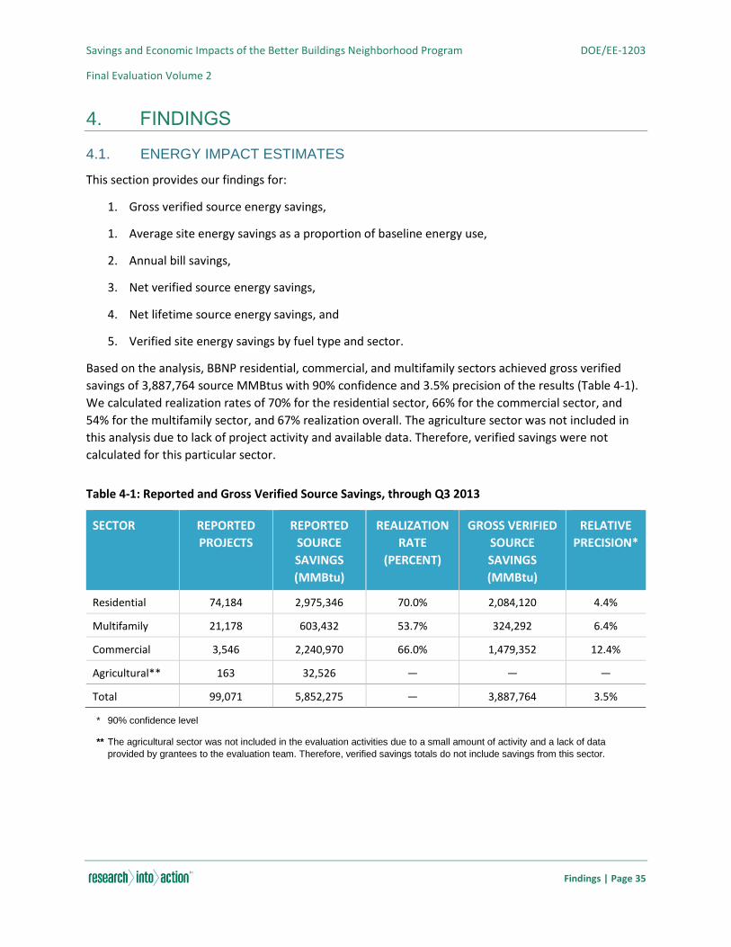
Savings and Economic Impacts of the Better Buildings Neighborhood Program DOE/EE-1203
Final Evaluation Volume 2
Findings | Page 35
4. FINDINGS
4.1. ENERGY IMPACT ESTIMATES
This section provides our findings for:
1. Gross verified source energy savings,
1. Average site energy savings as a proportion of baseline energy use,
2. Annual bill savings,
3. Net verified source energy savings,
4. Net lifetime source energy savings, and
5. Verified site energy savings by fuel type and sector.
Based on the analysis, BBNP residential, commercial, and multifamily sectors achieved gross verified
savings of 3,887,764 source MMBtus with 90% confidence and 3.5% precision of the results (Table 4-1).
We calculated realization rates of 70% for the residential sector, 66% for the commercial sector, and
54% for the multifamily sector, and 67% realization overall. The agriculture sector was not included in
this analysis due to lack of project activity and available data. Therefore, verified savings were not
calculated for this particular sector.
Table 4-1: Reported and Gross Verified Source Savings, through Q3 2013
SECTOR REPORTED
PROJECTS
REPORTED
SOURCE
SAVINGS
(MMBtu)
REALIZATION
RATE
(PERCENT)
GROSS VERIFIED
SOURCE
SAVINGS
(MMBtu)
RELATIVE
PRECISION*
Residential 74,184 2,975,346 70.0% 2,084,120 4.4%
Multifamily 21,178 603,432 53.7% 324,292 6.4%
Commercial 3,546 2,240,970 66.0% 1,479,352 12.4%
Agricultural** 163 32,526 — — —
Total 99,071 5,852,275 — 3,887,764 3.5%
* 90% confidence level
** The agricultural sector was not included in the evaluation activities due to a small amount of activity and a lack of data
provided by grantees to the evaluation team. Therefore, verified savings totals do not include savings from this sector.
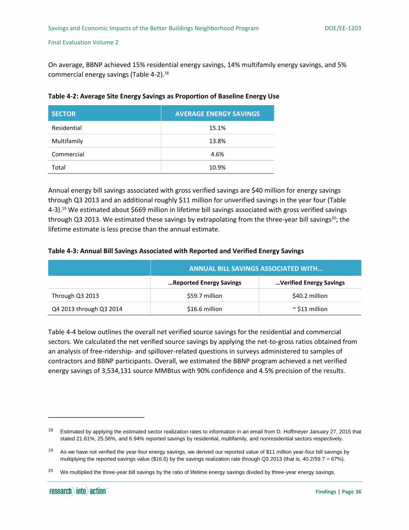
Savings and Economic Impacts of the Better Buildings Neighborhood Program DOE/EE-1203
Final Evaluation Volume 2
Findings | Page 36
On average, BBNP achieved 15% residential energy savings, 14% multifamily energy savings, and 5%
commercial energy savings (Table 4-2).18
Table 4-2: Average Site Energy Savings as Proportion of Baseline Energy Use
SECTOR AVERAGE ENERGY SAVINGS
Residential 15.1%
Multifamily 13.8%
Commercial 4.6%
Total 10.9%
Annual energy bill savings associated with gross verified savings are $40 million for energy savings
through Q3 2013 and an additional roughly $11 million for unverified savings in the year four (Table
4-3).19 We estimated about $669 million in lifetime bill savings associated with gross verified savings
through Q3 2013. We estimated these savings by extrapolating from the three-year bill savings20; the
lifetime estimate is less precise than the annual estimate.
Table 4-3: Annual Bill Savings Associated with Reported and Verified Energy Savings
ANNUAL BILL SAVINGS ASSOCIATED WITH…
…Reported Energy Savings …Verified Energy Savings
Through Q3 2013 $59.7 million $40.2 million
Q4 2013 through Q3 2014 $16.6 million ~ $11 million
Table 4-4 below outlines the overall net verified source savings for the residential and commercial
sectors. We calculated the net verified source savings by applying the net-to-gross ratios obtained from
an analysis of free-ridership- and spillover-related questions in surveys administered to samples of
contractors and BBNP participants. Overall, we estimated the BBNP program achieved a net verified
energy savings of 3,534,131 source MMBtus with 90% confidence and 4.5% precision of the results.
18 Estimated by applying the estimated sector realization rates to information in an email from D. Hoffmeyer January 27, 2015 that
stated 21.61%, 25.56%, and 6.94% reported savings by residential, multifamily, and nonresidential sectors respectively.
19 As we have not verified the year-four energy savings, we derived our reported value of $11 million year-four bill savings by
multiplying the reported savings value ($16.6) by the savings realization rate through Q3 2013 (that is, 40.2/59.7 = 67%).
20 We multiplied the three-year bill savings by the ratio of lifetime energy savings divided by three-year energy savings.
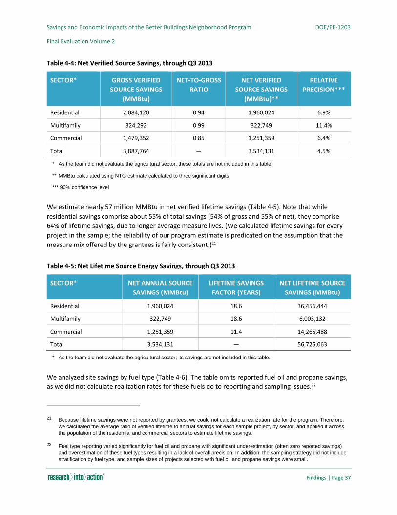
Savings and Economic Impacts of the Better Buildings Neighborhood Program DOE/EE-1203
Final Evaluation Volume 2
Findings | Page 37
Table 4-4: Net Verified Source Savings, through Q3 2013
SECTOR* GROSS VERIFIED
SOURCE SAVINGS
(MMBtu)
NET-TO-GROSS
RATIO
NET VERIFIED
SOURCE SAVINGS
(MMBtu)**
RELATIVE
PRECISION***
Residential 2,084,120 0.94 1,960,024 6.9%
Multifamily 324,292 0.99 322,749 11.4%
Commercial 1,479,352 0.85 1,251,359 6.4%
Total 3,887,764 — 3,534,131 4.5%
* As the team did not evaluate the agricultural sector, these totals are not included in this table.
** MMBtu calculated using NTG estimate calculated to three significant digits.
*** 90% confidence level
We estimate nearly 57 million MMBtu in net verified lifetime savings (Table 4-5). Note that while
residential savings comprise about 55% of total savings (54% of gross and 55% of net), they comprise
64% of lifetime savings, due to longer average measure lives. (We calculated lifetime savings for every
project in the sample; the reliability of our program estimate is predicated on the assumption that the
measure mix offered by the grantees is fairly consistent.)21
Table 4-5: Net Lifetime Source Energy Savings, through Q3 2013
SECTOR* NET ANNUAL SOURCE
SAVINGS (MMBtu)
LIFETIME SAVINGS
FACTOR (YEARS)
NET LIFETIME SOURCE
SAVINGS (MMBtu)
Residential 1,960,024 18.6 36,456,444
Multifamily 322,749 18.6 6,003,132
Commercial 1,251,359 11.4 14,265,488
Total 3,534,131 — 56,725,063
* As the team did not evaluate the agricultural sector; its savings are not included in this table.
We analyzed site savings by fuel type (Table 4-6). The table omits reported fuel oil and propane savings,
as we did not calculate realization rates for these fuels do to reporting and sampling issues.22
21 Because lifetime savings were not reported by grantees, we could not calculate a realization rate for the program. Therefore,
we calculated the average ratio of verified lifetime to annual savings for each sample project, by sector, and applied it across
the population of the residential and commercial sectors to estimate lifetime savings.
22 Fuel type reporting varied significantly for fuel oil and propane with significant underestimation (often zero reported savings)
and overestimation of these fuel types resulting in a lack of overall precision. In addition, the sampling strategy did not include
stratification by fuel type, and sample sizes of projects selected with fuel oil and propane savings were small.
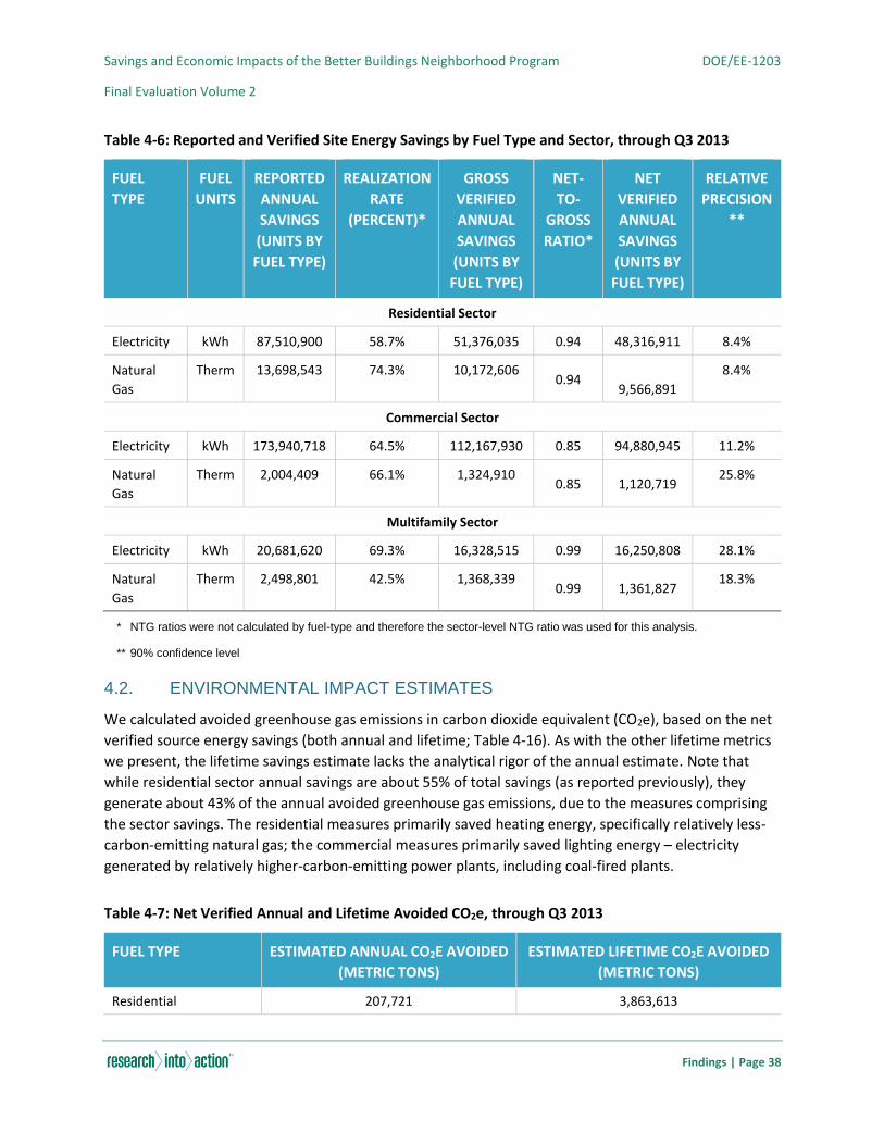
Savings and Economic Impacts of the Better Buildings Neighborhood Program DOE/EE-1203
Final Evaluation Volume 2
Findings | Page 38
Table 4-6: Reported and Verified Site Energy Savings by Fuel Type and Sector, through Q3 2013
FUEL
TYPE
FUEL
UNITS
REPORTED
ANNUAL
SAVINGS
(UNITS BY
FUEL TYPE)
REALIZATION
RATE
(PERCENT)*
GROSS
VERIFIED
ANNUAL
SAVINGS
(UNITS BY
FUEL TYPE)
NET-
TO-
GROSS
RATIO*
NET
VERIFIED
ANNUAL
SAVINGS
(UNITS BY
FUEL TYPE)
RELATIVE
PRECISION
**
Residential Sector
Electricity kWh 87,510,900 58.7% 51,376,035 0.94 48,316,911 8.4%
Natural
Gas
Therm 13,698,543 74.3% 10,172,606 0.94
9,566,891
8.4%
Commercial Sector
Electricity kWh 173,940,718 64.5% 112,167,930 0.85 94,880,945 11.2%
Natural
Gas
Therm 2,004,409 66.1% 1,324,910 0.85 1,120,719
25.8%
Multifamily Sector
Electricity kWh 20,681,620 69.3% 16,328,515 0.99 16,250,808 28.1%
Natural
Gas
Therm 2,498,801 42.5% 1,368,339 0.99 1,361,827
18.3%
* NTG ratios were not calculated by fuel-type and therefore the sector-level NTG ratio was used for this analysis.
** 90% confidence level
4.2. ENVIRONMENTAL IMPACT ESTIMATES
We calculated avoided greenhouse gas emissions in carbon dioxide equivalent (CO2e), based on the net
verified source energy savings (both annual and lifetime; Table 4-16). As with the other lifetime metrics
we present, the lifetime savings estimate lacks the analytical rigor of the annual estimate. Note that
while residential sector annual savings are about 55% of total savings (as reported previously), they
generate about 43% of the annual avoided greenhouse gas emissions, due to the measures comprising
the sector savings. The residential measures primarily saved heating energy, specifically relatively less-
carbon-emitting natural gas; the commercial measures primarily saved lighting energy – electricity
generated by relatively higher-carbon-emitting power plants, including coal-fired plants.
Table 4-7: Net Verified Annual and Lifetime Avoided CO2e, through Q3 2013
FUEL TYPE ESTIMATED ANNUAL CO2E AVOIDED
(METRIC TONS)
ESTIMATED LIFETIME CO2E AVOIDED
(METRIC TONS)
Residential 207,721 3,863,613
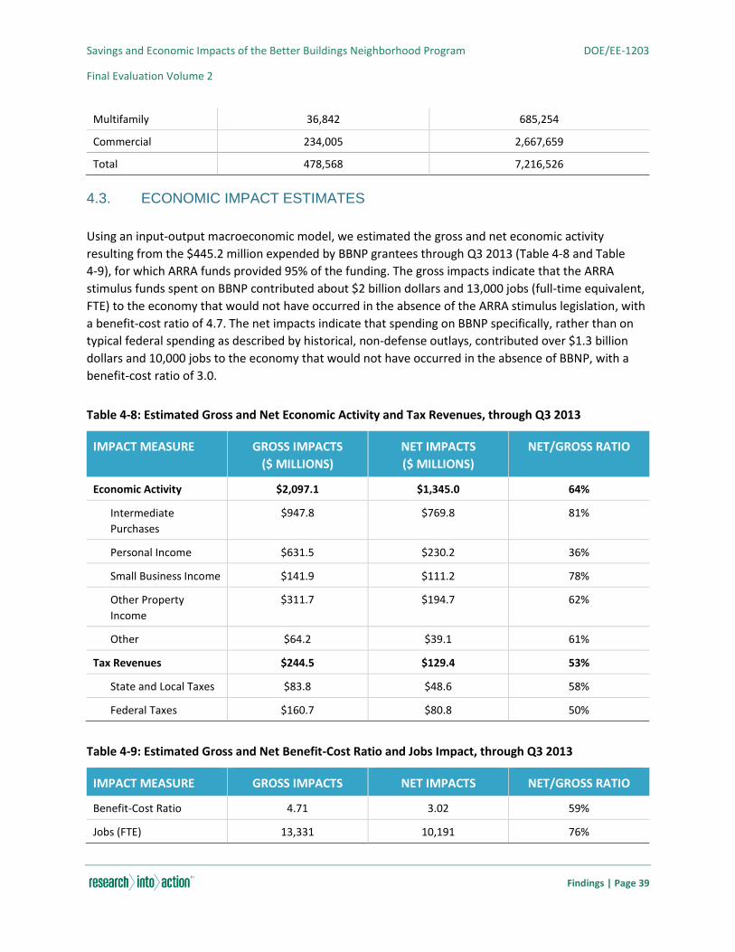
Savings and Economic Impacts of the Better Buildings Neighborhood Program DOE/EE-1203
Final Evaluation Volume 2
Findings | Page 39
Multifamily 36,842 685,254
Commercial 234,005 2,667,659
Total 478,568 7,216,526
4.3. ECONOMIC IMPACT ESTIMATES
Using an input-output macroeconomic model, we estimated the gross and net economic activity
resulting from the $445.2 million expended by BBNP grantees through Q3 2013 (Table 4-8 and Table
4-9), for which ARRA funds provided 95% of the funding. The gross impacts indicate that the ARRA
stimulus funds spent on BBNP contributed about $2 billion dollars and 13,000 jobs (full-time equivalent,
FTE) to the economy that would not have occurred in the absence of the ARRA stimulus legislation, with
a benefit-cost ratio of 4.7. The net impacts indicate that spending on BBNP specifically, rather than on
typical federal spending as described by historical, non-defense outlays, contributed over $1.3 billion
dollars and 10,000 jobs to the economy that would not have occurred in the absence of BBNP, with a
benefit-cost ratio of 3.0.
Table 4-8: Estimated Gross and Net Economic Activity and Tax Revenues, through Q3 2013
IMPACT MEASURE GROSS IMPACTS
($ MILLIONS)
NET IMPACTS
($ MILLIONS)
NET/GROSS RATIO
Economic Activity $2,097.1 $1,345.0 64%
Intermediate
Purchases
$947.8 $769.8 81%
Personal Income $631.5 $230.2 36%
Small Business Income $141.9 $111.2 78%
Other Property
Income
$311.7 $194.7 62%
Other $64.2 $39.1 61%
Tax Revenues $244.5 $129.4 53%
State and Local Taxes $83.8 $48.6 58%
Federal Taxes $160.7 $80.8 50%
Table 4-9: Estimated Gross and Net Benefit-Cost Ratio and Jobs Impact, through Q3 2013
IMPACT MEASURE GROSS IMPACTS NET IMPACTS NET/GROSS RATIO
Benefit-Cost Ratio 4.71 3.02 59%
Jobs (FTE) 13,331 10,191 76%
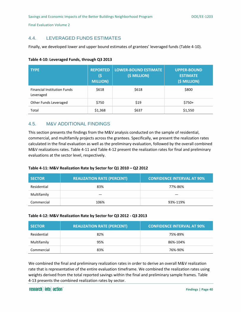
Savings and Economic Impacts of the Better Buildings Neighborhood Program DOE/EE-1203
Final Evaluation Volume 2
Findings | Page 40
4.4. LEVERAGED FUNDS ESTIMATES
Finally, we developed lower and upper bound estimates of grantees’ leveraged funds (Table 4-10).
Table 4-10: Leveraged Funds, through Q3 2013
TYPE REPORTED
($
MILLION)
LOWER-BOUND ESTIMATE
($ MILLION)
UPPER-BOUND
ESTIMATE
($ MILLION)
Financial Institution Funds
Leveraged
$618 $618 $800
Other Funds Leveraged $750 $19 $750+
Total $1,368 $637 $1,550
4.5. M&V ADDITIONAL FINDINGS
This section presents the findings from the M&V analysis conducted on the sample of residential,
commercial, and multifamily projects across the grantees. Specifically, we present the realization rates
calculated in the final evaluation as well as the preliminary evaluation, followed by the overall combined
M&V realizations rates. Table 4-11 and Table 4-12 present the realization rates for final and preliminary
evaluations at the sector level, respectively.
Table 4-11: M&V Realization Rate by Sector for Q1 2010 – Q2 2012
SECTOR REALIZATION RATE (PERCENT) CONFIDENCE INTERVAL AT 90%
Residential 83% 77%-86%
Multifamily — —
Commercial 106% 93%-119%
Table 4-12: M&V Realization Rate by Sector for Q3 2012 - Q3 2013
SECTOR REALIZATION RATE (PERCENT) CONFIDENCE INTERVAL AT 90%
Residential 82% 75%-89%
Multifamily 95% 86%-104%
Commercial 83% 76%-90%
We combined the final and preliminary realization rates in order to derive an overall M&V realization
rate that is representative of the entire evaluation timeframe. We combined the realization rates using
weights derived from the total reported savings within the final and preliminary sample frames. Table
4-13 presents the combined realization rates by sector.
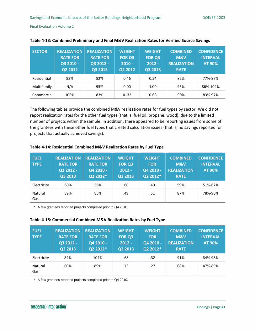
Savings and Economic Impacts of the Better Buildings Neighborhood Program DOE/EE-1203
Final Evaluation Volume 2
Findings | Page 41
Table 4-13: Combined Preliminary and Final M&V Realization Rates for Verified Source Savings
SECTOR REALIZATION
RATE FOR
Q3 2010 -
Q2 2012
REALIZATION
RATE FOR
Q3 2012 -
Q3 2013
WEIGHT
FOR Q3
2010 -
Q2 2012
WEIGHT
FOR Q3
2012 -
Q3 2013
COMBINED
M&V
REALIZATION
RATE
CONFIDENCE
INTERVAL
AT 90%
Residential 83% 82% 0.46 0.54 82% 77%-87%
Multifamily N/A 95% 0.00 1.00 95% 86%-104%
Commercial 106% 83% 0..32 0.68 90% 83%-97%
The following tables provide the combined M&V realization rates for fuel types by sector. We did not
report realization rates for the other fuel types (that is, fuel oil, propane, wood), due to the limited
number of projects within the sample. In addition, there appeared to be reporting issues from some of
the grantees with these other fuel types that created calculation issues (that is, no savings reported for
projects that actually achieved savings).
Table 4-14: Residential Combined M&V Realization Rates by Fuel Type
FUEL
TYPE
REALIZATION
RATE FOR
Q3 2012 -
Q3 2013
REALIZATION
RATE FOR
Q4 2010 -
Q2 2012*
WEIGHT
FOR Q3
2012 -
Q3 2013
WEIGHT
FOR
Q4 2010 -
Q2 2012*
COMBINED
M&V
REALIZATION
RATE
CONFIDENCE
INTERVAL
AT 90%
Electricity 60% 56% .60 .40 59% 51%-67%
Natural
Gas
89% 85% .49 .51 87% 78%-96%
* A few grantees reported projects completed prior to Q4 2010.
Table 4-15: Commercial Combined M&V Realization Rates by Fuel Type
FUEL
TYPE
REALIZATION
RATE FOR
Q3 2012 -
Q3 2013
REALIZATION
RATE FOR
Q4 2010 -
Q2 2012*
WEIGHT
FOR Q3
2012 -
Q3 2013
WEIGHT
FOR
Q4 2010 -
Q2 2012*
COMBINED
M&V
REALIZATION
RATE
CONFIDENCE
INTERVAL
AT 90%
Electricity 84% 104% .68 .32 91% 84%-98%
Natural
Gas
60% 89% .73 .27 68% 47%-89%
* A few grantees reported projects completed prior to Q4 2010.
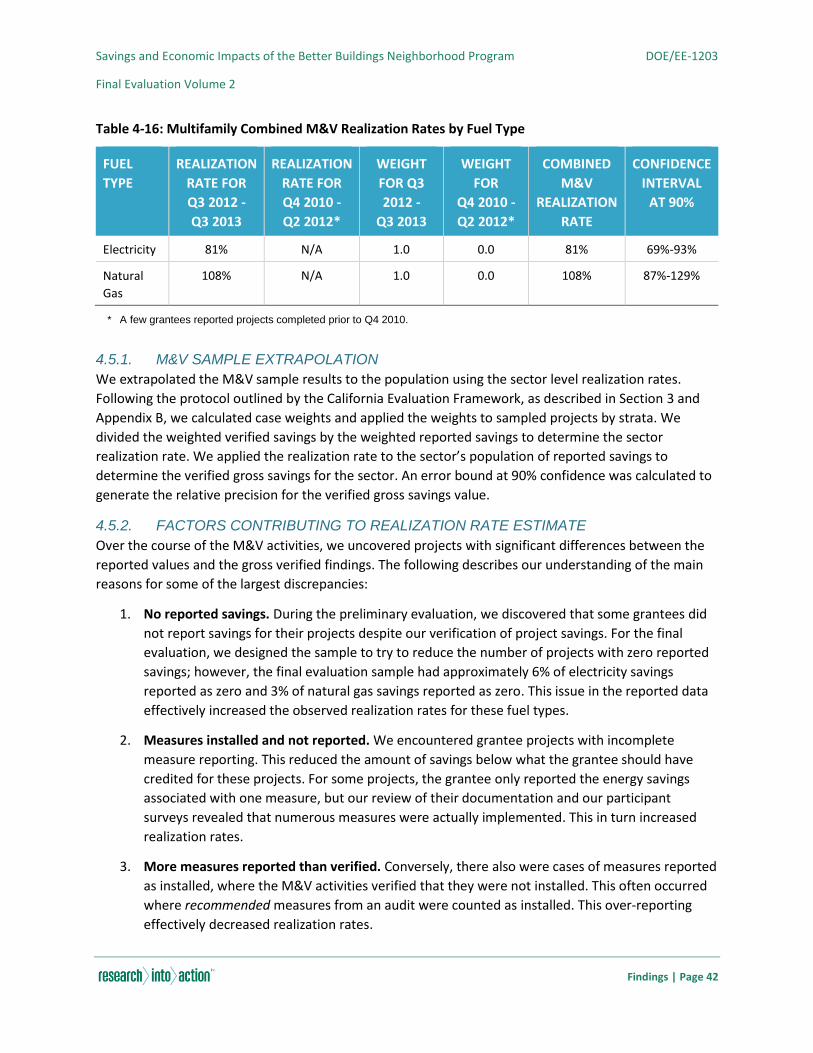
Savings and Economic Impacts of the Better Buildings Neighborhood Program DOE/EE-1203
Final Evaluation Volume 2
Findings | Page 42
Table 4-16: Multifamily Combined M&V Realization Rates by Fuel Type
FUEL
TYPE
REALIZATION
RATE FOR
Q3 2012 -
Q3 2013
REALIZATION
RATE FOR
Q4 2010 -
Q2 2012*
WEIGHT
FOR Q3
2012 -
Q3 2013
WEIGHT
FOR
Q4 2010 -
Q2 2012*
COMBINED
M&V
REALIZATION
RATE
CONFIDENCE
INTERVAL
AT 90%
Electricity 81% N/A 1.0 0.0 81% 69%-93%
Natural
Gas
108% N/A 1.0 0.0 108% 87%-129%
* A few grantees reported projects completed prior to Q4 2010.
4.5.1. M&V SAMPLE EXTRAPOLATION
We extrapolated the M&V sample results to the population using the sector level realization rates.
Following the protocol outlined by the California Evaluation Framework, as described in Section 3 and
Appendix B, we calculated case weights and applied the weights to sampled projects by strata. We
divided the weighted verified savings by the weighted reported savings to determine the sector
realization rate. We applied the realization rate to the sector’s population of reported savings to
determine the verified gross savings for the sector. An error bound at 90% confidence was calculated to
generate the relative precision for the verified gross savings value.
4.5.2. FACTORS CONTRIBUTING TO REALIZATION RATE ESTIMATE
Over the course of the M&V activities, we uncovered projects with significant differences between the
reported values and the gross verified findings. The following describes our understanding of the main
reasons for some of the largest discrepancies:
1. No reported savings. During the preliminary evaluation, we discovered that some grantees did
not report savings for their projects despite our verification of project savings. For the final
evaluation, we designed the sample to try to reduce the number of projects with zero reported
savings; however, the final evaluation sample had approximately 6% of electricity savings
reported as zero and 3% of natural gas savings reported as zero. This issue in the reported data
effectively increased the observed realization rates for these fuel types.
2. Measures installed and not reported. We encountered grantee projects with incomplete
measure reporting. This reduced the amount of savings below what the grantee should have
credited for these projects. For some projects, the grantee only reported the energy savings
associated with one measure, but our review of their documentation and our participant
surveys revealed that numerous measures were actually implemented. This in turn increased
realization rates.
3. More measures reported than verified. Conversely, there also were cases of measures reported
as installed, where the M&V activities verified that they were not installed. This often occurred
where recommended measures from an audit were counted as installed. This over-reporting
effectively decreased realization rates.

Savings and Economic Impacts of the Better Buildings Neighborhood Program DOE/EE-1203
Final Evaluation Volume 2
Findings | Page 43
4. Overstatement of savings. In a few cases, we identified issues where the energy savings being
reported by the grantee was more energy than was actually consumed by a typical customer.
This over-reporting also decreased realization rates. This over-reporting likely was due to energy
modeling issues, but because the models could not be calibrated or the inputs verified, it was
difficult to know the exact reasons. Additionally, savings may have been overstated due to
inaccurate deemed savings applied to project measures.
5. Heat pump installations. We encountered projects that resulted in the replacement of a
primary heating system, such as a natural gas furnace or resistance heater, with heat pumps.
Project documentation usually calculated savings as the displaced energy consumption of the
previous system; however, documentation was often lacking regarding the energy consumption
of the new heat pump especially for the potential new cooling load provided by the heat pump.
6. Fuel type reporting issues. There were cases where grantees reported fuel type savings
incorrectly, either by listing the wrong fuel type or listing the wrong units (that is, MMBtu
instead of kWh).
4.6. BILLING REGRESSION ANALYSIS FINDINGS
This section presents the results from the billing regression models and the resulting savings estimates
for the grantees included in the billing regression analysis. Table 4-19 presents the sector level model
results for both the electric and gas models with additional detail provided in B.10.
4.6.1. FINAL MODEL SPECIFICATION RESULTS
In general, our model results were consistent with expectations. Most coefficients had statistically
significant estimates and were of expected magnitude. The variable of interest was Post, which
represented the change in consumption in the post-retrofit installation period and, therefore, was a
reflection of energy savings resulting from the program and other factors. As shown in Table 4-17, the
point estimate of -76.27 in the residential electric model indicates energy savings of about 76 kWh per
month or 8.1% of pre-retrofit monthly electricity consumption holding all other terms constant. The
point estimate of -274.36 in the commercial electric model indicates energy savings of around 274 kWh
per month or 12.1% of pre-retrofit monthly/annual electricity consumption holding all other terms
constant. These models were only free of bias to the extent that billing histories not suitable for the
analyses were any different from those included.
Table 4-17: Electricity Billing Regression Model Output
VARIABLE COEFFICIENT
(𝜷)
STANDARD
ERROR
𝜷/STANDARD
ERROR
PROBABILITY
[|Z|>Z]
95% CONFIDENCE
INTERVAL
(𝛃𝟏) Post -76.2730 1.8493 -41.2445 0.00% (-79.898, -72.648)
(𝛃𝟐) HDD 0.3288 0.0068 48.5984 0.00% (0.316, 0.342)
(𝛃𝟑) CDD 1.7811 0.0130 137.2140 0.00% (1.756, 1.807)
(𝜷𝟒) January 58.2920 4.8647 11.9827 0.00% (48.757, 67.827)
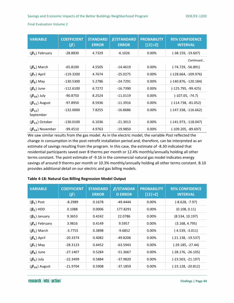
Savings and Economic Impacts of the Better Buildings Neighborhood Program DOE/EE-1203
Final Evaluation Volume 2
Findings | Page 44
VARIABLE COEFFICIENT
(𝜷)
STANDARD
ERROR
𝜷/STANDARD
ERROR
PROBABILITY
[|Z|>Z]
95% CONFIDENCE
INTERVAL
(𝜷𝟓) February -28.8830 4.7329 -6.1026 0.00% (-38.159, -19.607)
Continued…
(𝜷𝟔) March -65.8100 4.5505 -14.4619 0.00% (-74.729, -56.891)
(𝜷𝟕) April -119.3200 4.7674 -25.0275 0.00% (-128.664, -109.976)
(𝜷𝟖) May -130.5300 5.2786 -24.7291 0.00% (-140.876, -120.184)
(𝜷𝟗) June -112.6100 6.7272 -16.7390 0.00% (-125.795, -99.425)
(𝜷𝟏𝟎) July -90.8750 8.2524 -11.0119 0.00% (-107.05, -74.7)
(𝜷𝟏𝟏) August -97.8950 8.5936 -11.3916 0.00% (-114.738, -81.052)
(𝜷𝟏𝟐)
September
-132.0000 7.8255 -16.8686 0.00% (-147.338, -116.662)
(𝜷𝟏𝟑) October -130.0100 6.1036 -21.3013 0.00% (-141.973, -118.047)
(𝜷𝟏𝟒) November -99.4510 4.9763 -19.9850 0.00% (-109.205, -89.697)
We saw similar results from the gas model. As in the electric model, the variable Post reflected the
change in consumption in the post-retrofit installation period and, therefore, can be interpreted as an
estimate of savings resulting from the program. In this case, the estimate of -8.30 indicated that
residential participants saved over 8 therms per month or 12.4% monthly/annually holding all other
terms constant. The point estimate of -9.16 in the commercial natural gas model indicates energy
savings of around 9 therms per month or 10.3% monthly/annually holding all other terms constant. B.10
provides additional detail on our electric and gas billing models.
Table 4-18: Natural Gas Billing Regression Model Output
VARIABLE COEFFICIENT
(𝜷)
STANDARD
ERROR
𝜷/STANDAR
D ERROR
PROBABILITY
[|Z|>Z]
95% CONFIDENCE
INTERVAL
(𝛃𝟏) Post -8.2989 0.1678 -49.4444 0.00% (-8.628, -7.97)
(𝛃𝟐) HDD 0.1088 0.0006 177.8291 0.00% (0.108, 0.11)
(𝛃𝟑) January 9.3653 0.4242 22.0786 0.00% (8.534, 10.197)
(𝜷𝟒) February 3.9816 0.4149 9.5957 0.00% (3.168, 4.795)
(𝜷𝟓) March -3.7755 0.3898 -9.6852 0.00% (-4.539, -3.011)
(𝜷𝟔) April -20.3374 0.4082 -49.8206 0.00% (-21.138, -19.537)
(𝜷𝟕) May -28.3123 0.4452 -63.5943 0.00% (-29.185, -27.44)
(𝜷𝟖) June -27.1407 0.5284 -51.3667 0.00% (-28.176, -26.105)
(𝜷𝟗) July -22.3499 0.5884 -37.9820 0.00% (-23.503, -21.197)
(𝜷𝟏𝟎) August -21.9704 0.5908 -37.1859 0.00% (-23.128, -20.812)
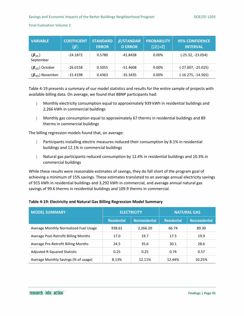
Savings and Economic Impacts of the Better Buildings Neighborhood Program DOE/EE-1203
Final Evaluation Volume 2
Findings | Page 45
VARIABLE COEFFICIENT
(𝜷)
STANDARD
ERROR
𝜷/STANDAR
D ERROR
PROBABILITY
[|Z|>Z]
95% CONFIDENCE
INTERVAL
(𝜷𝟏𝟏)
September
-24.1872 0.5780 -41.8438 0.00% (-25.32, -23.054)
(𝜷𝟏𝟐) October -26.0158 0.5055 -51.4608 0.00% (-27.007, -25.025)
(𝜷𝟏𝟑) November -15.4198 0.4363 -35.3435 0.00% (-16.275, -14.565)
Table 4-19 presents a summary of our model statistics and results for the entire sample of projects with
available billing data. On average, we found that BBNP participants had:
Monthly electricity consumption equal to approximately 939 kWh in residential buildings and
2,266 kWh in commercial buildings
Monthly gas consumption equal to approximately 67 therms in residential buildings and 89
therms in commercial buildings
The billing regression models found that, on average:
Participants installing electric measures reduced their consumption by 8.1% in residential
buildings and 12.1% in commercial buildings
Natural gas participants reduced consumption by 12.4% in residential buildings and 10.3% in
commercial buildings
While these results were reasonable estimates of savings, they do fall short of the program goal of
achieving a minimum of 15% savings. These estimates translated to an average annual electricity savings
of 915 kWh in residential buildings and 3,292 kWh in commercial, and average annual natural gas
savings of 99.6 therms in residential buildings and 109.9 therms in commercial.
Table 4-19: Electricity and Natural Gas Billing Regression Model Summary
MODEL SUMMARY ELECTRICITY NATURAL GAS
Residential Nonresidential Residential Nonresidential
Average Monthly Normalized Fuel Usage 938.61 2,266.20 66.74 89.30
Average Post-Retrofit Billing Months 17.0 19.7 17.5 19.9
Average Pre-Retrofit Billing Months 24.5 35.6 30.1 28.6
Adjusted R-Squared Statistic 0.25 0.25 0.74 0.57
Average Monthly Savings (% of usage) 8.13% 12.11% 12.44% 10.25%
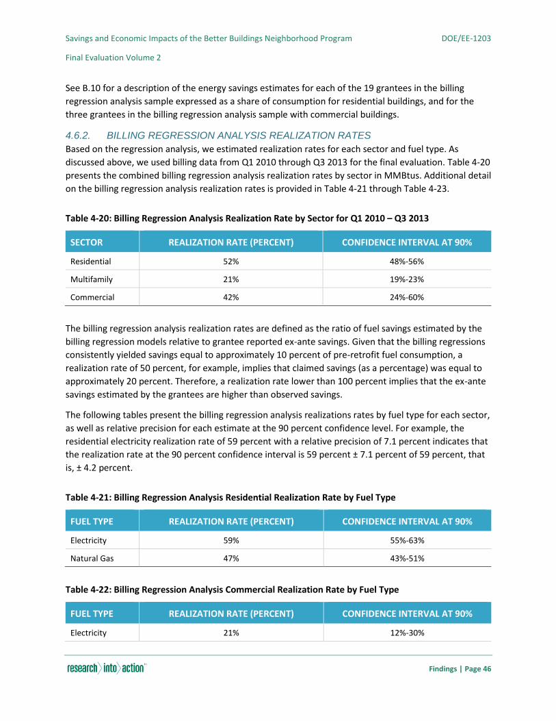
Savings and Economic Impacts of the Better Buildings Neighborhood Program DOE/EE-1203
Final Evaluation Volume 2
Findings | Page 46
See B.10 for a description of the energy savings estimates for each of the 19 grantees in the billing
regression analysis sample expressed as a share of consumption for residential buildings, and for the
three grantees in the billing regression analysis sample with commercial buildings.
4.6.2. BILLING REGRESSION ANALYSIS REALIZATION RATES
Based on the regression analysis, we estimated realization rates for each sector and fuel type. As
discussed above, we used billing data from Q1 2010 through Q3 2013 for the final evaluation. Table 4-20
presents the combined billing regression analysis realization rates by sector in MMBtus. Additional detail
on the billing regression analysis realization rates is provided in Table 4-21 through Table 4-23.
Table 4-20: Billing Regression Analysis Realization Rate by Sector for Q1 2010 – Q3 2013
SECTOR REALIZATION RATE (PERCENT) CONFIDENCE INTERVAL AT 90%
Residential 52% 48%-56%
Multifamily 21% 19%-23%
Commercial 42% 24%-60%
The billing regression analysis realization rates are defined as the ratio of fuel savings estimated by the
billing regression models relative to grantee reported ex-ante savings. Given that the billing regressions
consistently yielded savings equal to approximately 10 percent of pre-retrofit fuel consumption, a
realization rate of 50 percent, for example, implies that claimed savings (as a percentage) was equal to
approximately 20 percent. Therefore, a realization rate lower than 100 percent implies that the ex-ante
savings estimated by the grantees are higher than observed savings.
The following tables present the billing regression analysis realizations rates by fuel type for each sector,
as well as relative precision for each estimate at the 90 percent confidence level. For example, the
residential electricity realization rate of 59 percent with a relative precision of 7.1 percent indicates that
the realization rate at the 90 percent confidence interval is 59 percent ± 7.1 percent of 59 percent, that
is, ± 4.2 percent.
Table 4-21: Billing Regression Analysis Residential Realization Rate by Fuel Type
FUEL TYPE REALIZATION RATE (PERCENT) CONFIDENCE INTERVAL AT 90%
Electricity 59% 55%-63%
Natural Gas 47% 43%-51%
Table 4-22: Billing Regression Analysis Commercial Realization Rate by Fuel Type
FUEL TYPE REALIZATION RATE (PERCENT) CONFIDENCE INTERVAL AT 90%
Electricity 21% 12%-30%
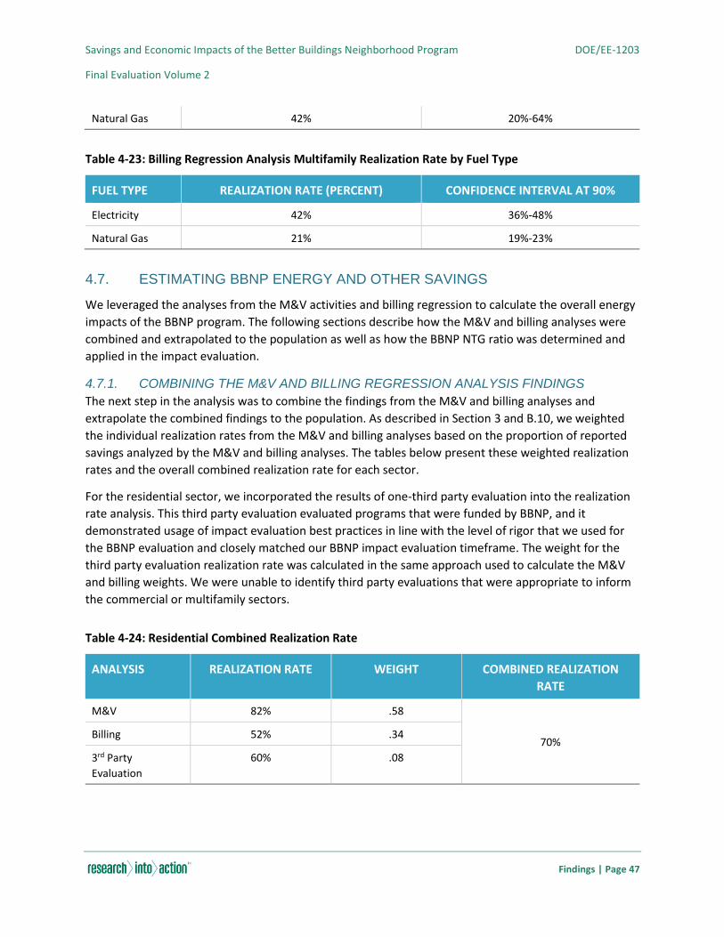
Savings and Economic Impacts of the Better Buildings Neighborhood Program DOE/EE-1203
Final Evaluation Volume 2
Findings | Page 47
Natural Gas 42% 20%-64%
Table 4-23: Billing Regression Analysis Multifamily Realization Rate by Fuel Type
FUEL TYPE REALIZATION RATE (PERCENT) CONFIDENCE INTERVAL AT 90%
Electricity 42% 36%-48%
Natural Gas 21% 19%-23%
4.7. ESTIMATING BBNP ENERGY AND OTHER SAVINGS
We leveraged the analyses from the M&V activities and billing regression to calculate the overall energy
impacts of the BBNP program. The following sections describe how the M&V and billing analyses were
combined and extrapolated to the population as well as how the BBNP NTG ratio was determined and
applied in the impact evaluation.
4.7.1. COMBINING THE M&V AND BILLING REGRESSION ANALYSIS FINDINGS
The next step in the analysis was to combine the findings from the M&V and billing analyses and
extrapolate the combined findings to the population. As described in Section 3 and B.10, we weighted
the individual realization rates from the M&V and billing analyses based on the proportion of reported
savings analyzed by the M&V and billing analyses. The tables below present these weighted realization
rates and the overall combined realization rate for each sector.
For the residential sector, we incorporated the results of one-third party evaluation into the realization
rate analysis. This third party evaluation evaluated programs that were funded by BBNP, and it
demonstrated usage of impact evaluation best practices in line with the level of rigor that we used for
the BBNP evaluation and closely matched our BBNP impact evaluation timeframe. The weight for the
third party evaluation realization rate was calculated in the same approach used to calculate the M&V
and billing weights. We were unable to identify third party evaluations that were appropriate to inform
the commercial or multifamily sectors.
Table 4-24: Residential Combined Realization Rate
ANALYSIS REALIZATION RATE WEIGHT COMBINED REALIZATION
RATE
M&V 82% .58
70% Billing 52% .34
3rd Party
Evaluation
60% .08
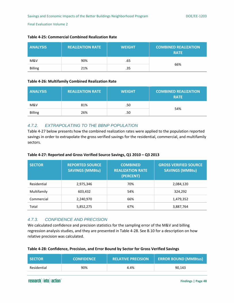
Savings and Economic Impacts of the Better Buildings Neighborhood Program DOE/EE-1203
Final Evaluation Volume 2
Findings | Page 48
Table 4-25: Commercial Combined Realization Rate
ANALYSIS REALIZATION RATE WEIGHT COMBINED REALIZATION
RATE
M&V 90% .65 66%
Billing 21% .35
Table 4-26: Multifamily Combined Realization Rate
ANALYSIS REALIZATION RATE WEIGHT COMBINED REALIZATION
RATE
M&V 81% .50 54%
Billing 26% .50
4.7.2. EXTRAPOLATING TO THE BBNP POPULATION
Table 4-27 below presents how the combined realization rates were applied to the population reported
savings in order to extrapolate the gross verified savings for the residential, commercial, and multifamily
sectors.
Table 4-27: Reported and Gross Verified Source Savings, Q1 2010 – Q3 2013
SECTOR REPORTED SOURCE
SAVINGS (MMBtu)
COMBINED
REALIZATION RATE
(PERCENT)
GROSS VERIFIED SOURCE
SAVINGS (MMBtu)
Residential 2,975,346 70% 2,084,120
Multifamily 603,432 54% 324,292
Commercial 2,240,970 66% 1,479,352
Total 5,852,275 67% 3,887,764
4.7.3. CONFIDENCE AND PRECISION
We calculated confidence and precision statistics for the sampling error of the M&V and billing
regression analysis studies, and they are presented in Table 4-28. See B.10 for a description on how
relative precision was calculated.
Table 4-28: Confidence, Precision, and Error Bound by Sector for Gross Verified Savings
SECTOR CONFIDENCE RELATIVE PRECISION ERROR BOUND (MMBtus)
Residential 90% 4.4% 90,143
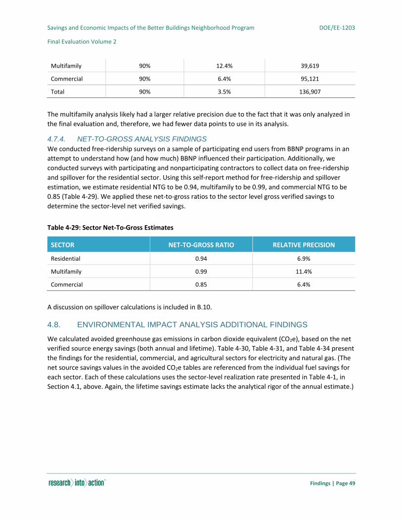
Savings and Economic Impacts of the Better Buildings Neighborhood Program DOE/EE-1203
Final Evaluation Volume 2
Findings | Page 49
Multifamily 90% 12.4% 39,619
Commercial 90% 6.4% 95,121
Total 90% 3.5% 136,907
The multifamily analysis likely had a larger relative precision due to the fact that it was only analyzed in
the final evaluation and, therefore, we had fewer data points to use in its analysis.
4.7.4. NET-TO-GROSS ANALYSIS FINDINGS
We conducted free-ridership surveys on a sample of participating end users from BBNP programs in an
attempt to understand how (and how much) BBNP influenced their participation. Additionally, we
conducted surveys with participating and nonparticipating contractors to collect data on free-ridership
and spillover for the residential sector. Using this self-report method for free-ridership and spillover
estimation, we estimate residential NTG to be 0.94, multifamily to be 0.99, and commercial NTG to be
0.85 (Table 4-29). We applied these net-to-gross ratios to the sector level gross verified savings to
determine the sector-level net verified savings.
Table 4-29: Sector Net-To-Gross Estimates
SECTOR NET-TO-GROSS RATIO RELATIVE PRECISION
Residential 0.94 6.9%
Multifamily 0.99 11.4%
Commercial 0.85 6.4%
A discussion on spillover calculations is included in B.10.
4.8. ENVIRONMENTAL IMPACT ANALYSIS ADDITIONAL FINDINGS
We calculated avoided greenhouse gas emissions in carbon dioxide equivalent (CO2e), based on the net
verified source energy savings (both annual and lifetime). Table 4-30, Table 4-31, and Table 4-34 present
the findings for the residential, commercial, and agricultural sectors for electricity and natural gas. (The
net source savings values in the avoided CO2e tables are referenced from the individual fuel savings for
each sector. Each of these calculations uses the sector-level realization rate presented in Table 4-1, in
Section 4.1, above. Again, the lifetime savings estimate lacks the analytical rigor of the annual estimate.)
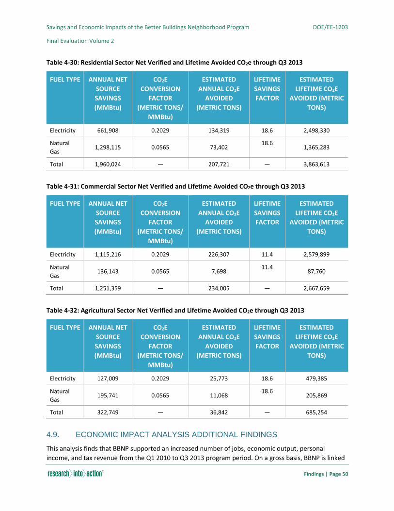
Savings and Economic Impacts of the Better Buildings Neighborhood Program DOE/EE-1203
Final Evaluation Volume 2
Findings | Page 50
Table 4-30: Residential Sector Net Verified and Lifetime Avoided CO2e through Q3 2013
FUEL TYPE ANNUAL NET
SOURCE
SAVINGS
(MMBtu)
CO2E
CONVERSION
FACTOR
(METRIC TONS/
MMBtu)
ESTIMATED
ANNUAL CO2E
AVOIDED
(METRIC TONS)
LIFETIME
SAVINGS
FACTOR
ESTIMATED
LIFETIME CO2E
AVOIDED (METRIC
TONS)
Electricity 661,908 0.2029 134,319 18.6 2,498,330
Natural
Gas 1,298,115 0.0565 73,402
18.6 1,365,283
Total 1,960,024 — 207,721 — 3,863,613
Table 4-31: Commercial Sector Net Verified and Lifetime Avoided CO2e through Q3 2013
FUEL TYPE ANNUAL NET
SOURCE
SAVINGS
(MMBtu)
CO2E
CONVERSION
FACTOR
(METRIC TONS/
MMBtu)
ESTIMATED
ANNUAL CO2E
AVOIDED
(METRIC TONS)
LIFETIME
SAVINGS
FACTOR
ESTIMATED
LIFETIME CO2E
AVOIDED (METRIC
TONS)
Electricity 1,115,216 0.2029 226,307 11.4 2,579,899
Natural
Gas 136,143 0.0565 7,698
11.4 87,760
Total 1,251,359 — 234,005 — 2,667,659
Table 4-32: Agricultural Sector Net Verified and Lifetime Avoided CO2e through Q3 2013
FUEL TYPE ANNUAL NET
SOURCE
SAVINGS
(MMBtu)
CO2E
CONVERSION
FACTOR
(METRIC TONS/
MMBtu)
ESTIMATED
ANNUAL CO2E
AVOIDED
(METRIC TONS)
LIFETIME
SAVINGS
FACTOR
ESTIMATED
LIFETIME CO2E
AVOIDED (METRIC
TONS)
Electricity 127,009 0.2029 25,773 18.6 479,385
Natural
Gas 195,741 0.0565 11,068
18.6 205,869
Total 322,749 — 36,842 — 685,254
4.9. ECONOMIC IMPACT ANALYSIS ADDITIONAL FINDINGS
This analysis finds that BBNP supported an increased number of jobs, economic output, personal
income, and tax revenue from the Q1 2010 to Q3 2013 program period. On a gross basis, BBNP is linked
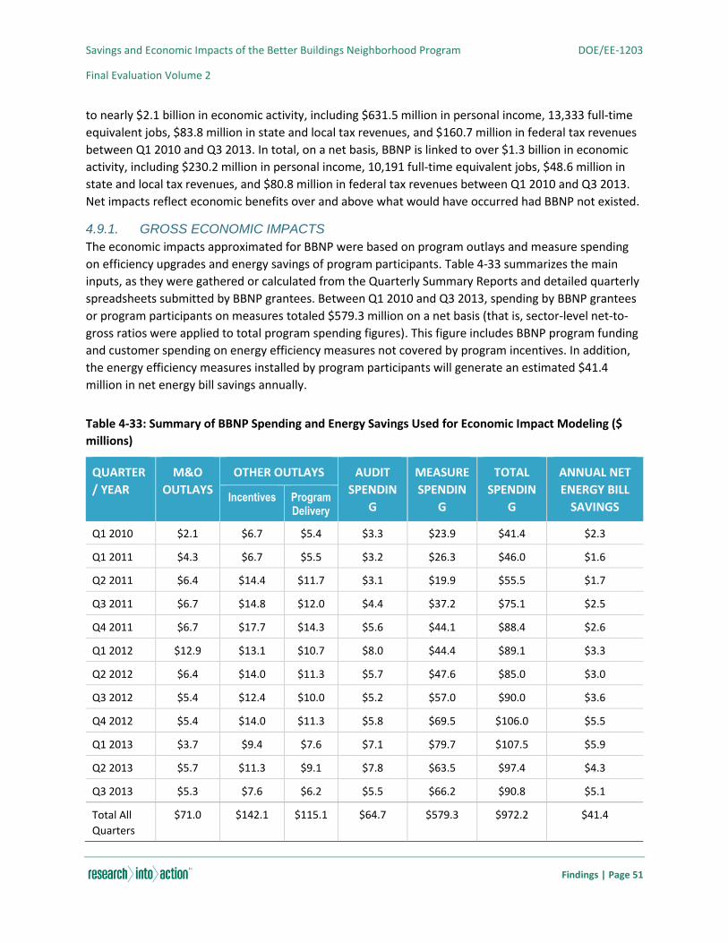
Savings and Economic Impacts of the Better Buildings Neighborhood Program DOE/EE-1203
Final Evaluation Volume 2
Findings | Page 51
to nearly $2.1 billion in economic activity, including $631.5 million in personal income, 13,333 full-time
equivalent jobs, $83.8 million in state and local tax revenues, and $160.7 million in federal tax revenues
between Q1 2010 and Q3 2013. In total, on a net basis, BBNP is linked to over $1.3 billion in economic
activity, including $230.2 million in personal income, 10,191 full-time equivalent jobs, $48.6 million in
state and local tax revenues, and $80.8 million in federal tax revenues between Q1 2010 and Q3 2013.
Net impacts reflect economic benefits over and above what would have occurred had BBNP not existed.
4.9.1. GROSS ECONOMIC IMPACTS
The economic impacts approximated for BBNP were based on program outlays and measure spending
on efficiency upgrades and energy savings of program participants. Table 4-33 summarizes the main
inputs, as they were gathered or calculated from the Quarterly Summary Reports and detailed quarterly
spreadsheets submitted by BBNP grantees. Between Q1 2010 and Q3 2013, spending by BBNP grantees
or program participants on measures totaled $579.3 million on a net basis (that is, sector-level net-to-
gross ratios were applied to total program spending figures). This figure includes BBNP program funding
and customer spending on energy efficiency measures not covered by program incentives. In addition,
the energy efficiency measures installed by program participants will generate an estimated $41.4
million in net energy bill savings annually.
Table 4-33: Summary of BBNP Spending and Energy Savings Used for Economic Impact Modeling ($
millions)
QUARTER
/ YEAR
M&O
OUTLAYS
OTHER OUTLAYS AUDIT
SPENDIN
G
MEASURE
SPENDIN
G
TOTAL
SPENDIN
G
ANNUAL NET
ENERGY BILL
SAVINGS Incentives Program
Delivery
Q1 2010 $2.1 $6.7 $5.4 $3.3 $23.9 $41.4 $2.3
Q1 2011 $4.3 $6.7 $5.5 $3.2 $26.3 $46.0 $1.6
Q2 2011 $6.4 $14.4 $11.7 $3.1 $19.9 $55.5 $1.7
Q3 2011 $6.7 $14.8 $12.0 $4.4 $37.2 $75.1 $2.5
Q4 2011 $6.7 $17.7 $14.3 $5.6 $44.1 $88.4 $2.6
Q1 2012 $12.9 $13.1 $10.7 $8.0 $44.4 $89.1 $3.3
Q2 2012 $6.4 $14.0 $11.3 $5.7 $47.6 $85.0 $3.0
Q3 2012 $5.4 $12.4 $10.0 $5.2 $57.0 $90.0 $3.6
Q4 2012 $5.4 $14.0 $11.3 $5.8 $69.5 $106.0 $5.5
Q1 2013 $3.7 $9.4 $7.6 $7.1 $79.7 $107.5 $5.9
Q2 2013 $5.7 $11.3 $9.1 $7.8 $63.5 $97.4 $4.3
Q3 2013 $5.3 $7.6 $6.2 $5.5 $66.2 $90.8 $5.1
Total All
Quarters
$71.0 $142.1 $115.1 $64.7 $579.3 $972.2 $41.4
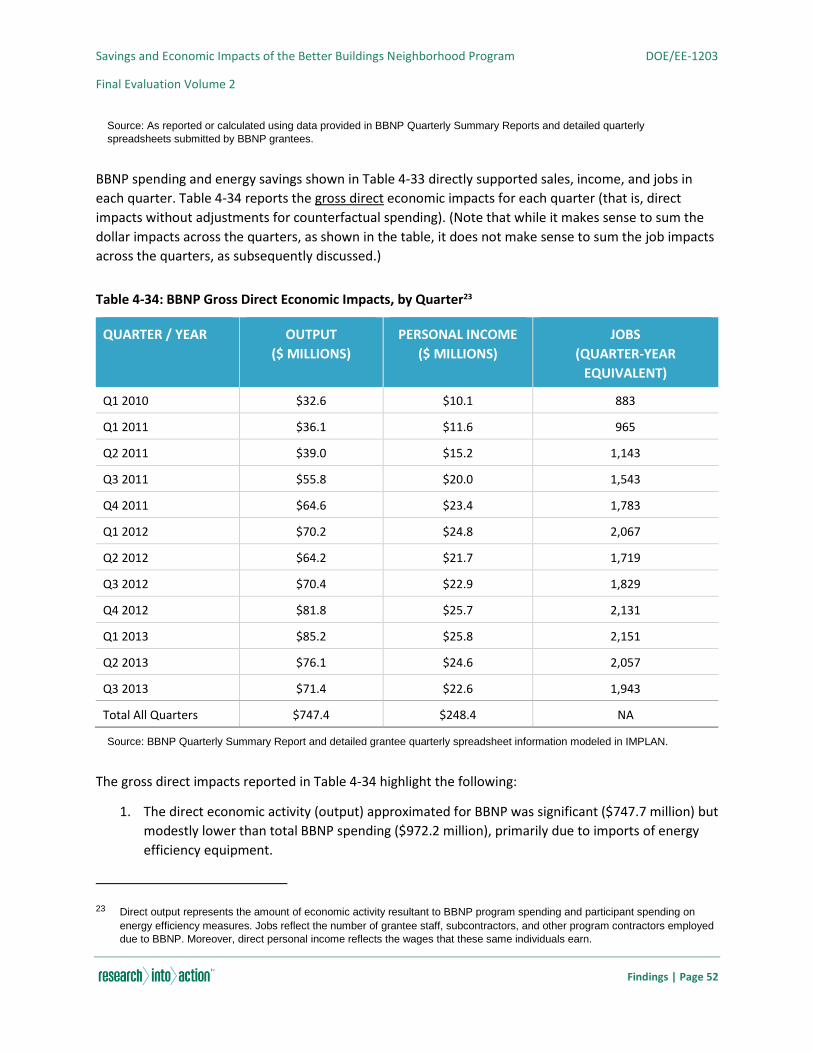
Savings and Economic Impacts of the Better Buildings Neighborhood Program DOE/EE-1203
Final Evaluation Volume 2
Findings | Page 52
Source: As reported or calculated using data provided in BBNP Quarterly Summary Reports and detailed quarterly
spreadsheets submitted by BBNP grantees.
BBNP spending and energy savings shown in Table 4-33 directly supported sales, income, and jobs in
each quarter. Table 4-34 reports the gross direct economic impacts for each quarter (that is, direct
impacts without adjustments for counterfactual spending). (Note that while it makes sense to sum the
dollar impacts across the quarters, as shown in the table, it does not make sense to sum the job impacts
across the quarters, as subsequently discussed.)
Table 4-34: BBNP Gross Direct Economic Impacts, by Quarter23
QUARTER / YEAR OUTPUT
($ MILLIONS)
PERSONAL INCOME
($ MILLIONS)
JOBS
(QUARTER-YEAR
EQUIVALENT)
Q1 2010 $32.6 $10.1 883
Q1 2011 $36.1 $11.6 965
Q2 2011 $39.0 $15.2 1,143
Q3 2011 $55.8 $20.0 1,543
Q4 2011 $64.6 $23.4 1,783
Q1 2012 $70.2 $24.8 2,067
Q2 2012 $64.2 $21.7 1,719
Q3 2012 $70.4 $22.9 1,829
Q4 2012 $81.8 $25.7 2,131
Q1 2013 $85.2 $25.8 2,151
Q2 2013 $76.1 $24.6 2,057
Q3 2013 $71.4 $22.6 1,943
Total All Quarters $747.4 $248.4 NA
Source: BBNP Quarterly Summary Report and detailed grantee quarterly spreadsheet information modeled in IMPLAN.
The gross direct impacts reported in Table 4-34 highlight the following:
1. The direct economic activity (output) approximated for BBNP was significant ($747.7 million) but
modestly lower than total BBNP spending ($972.2 million), primarily due to imports of energy
efficiency equipment.
23 Direct output represents the amount of economic activity resultant to BBNP program spending and participant spending on
energy efficiency measures. Jobs reflect the number of grantee staff, subcontractors, and other program contractors employed
due to BBNP. Moreover, direct personal income reflects the wages that these same individuals earn.
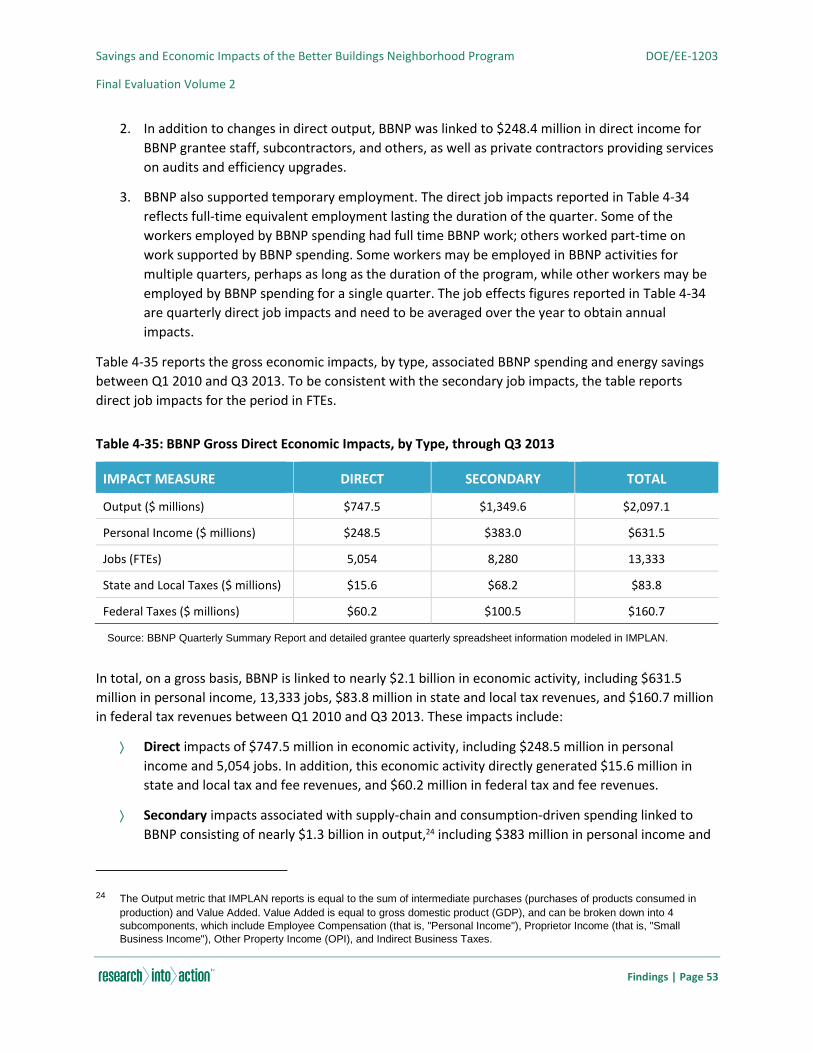
Savings and Economic Impacts of the Better Buildings Neighborhood Program DOE/EE-1203
Final Evaluation Volume 2
Findings | Page 53
2. In addition to changes in direct output, BBNP was linked to $248.4 million in direct income for
BBNP grantee staff, subcontractors, and others, as well as private contractors providing services
on audits and efficiency upgrades.
3. BBNP also supported temporary employment. The direct job impacts reported in Table 4-34
reflects full-time equivalent employment lasting the duration of the quarter. Some of the
workers employed by BBNP spending had full time BBNP work; others worked part-time on
work supported by BBNP spending. Some workers may be employed in BBNP activities for
multiple quarters, perhaps as long as the duration of the program, while other workers may be
employed by BBNP spending for a single quarter. The job effects figures reported in Table 4-34
are quarterly direct job impacts and need to be averaged over the year to obtain annual
impacts.
Table 4-35 reports the gross economic impacts, by type, associated BBNP spending and energy savings
between Q1 2010 and Q3 2013. To be consistent with the secondary job impacts, the table reports
direct job impacts for the period in FTEs.
Table 4-35: BBNP Gross Direct Economic Impacts, by Type, through Q3 2013
IMPACT MEASURE DIRECT SECONDARY TOTAL
Output ($ millions) $747.5 $1,349.6 $2,097.1
Personal Income ($ millions) $248.5 $383.0 $631.5
Jobs (FTEs) 5,054 8,280 13,333
State and Local Taxes ($ millions) $15.6 $68.2 $83.8
Federal Taxes ($ millions) $60.2 $100.5 $160.7
Source: BBNP Quarterly Summary Report and detailed grantee quarterly spreadsheet information modeled in IMPLAN.
In total, on a gross basis, BBNP is linked to nearly $2.1 billion in economic activity, including $631.5
million in personal income, 13,333 jobs, $83.8 million in state and local tax revenues, and $160.7 million
in federal tax revenues between Q1 2010 and Q3 2013. These impacts include:
Direct impacts of $747.5 million in economic activity, including $248.5 million in personal
income and 5,054 jobs. In addition, this economic activity directly generated $15.6 million in
state and local tax and fee revenues, and $60.2 million in federal tax and fee revenues.
Secondary impacts associated with supply-chain and consumption-driven spending linked to
BBNP consisting of nearly $1.3 billion in output,24 including $383 million in personal income and
24 The Output metric that IMPLAN reports is equal to the sum of intermediate purchases (purchases of products consumed in
production) and Value Added. Value Added is equal to gross domestic product (GDP), and can be broken down into 4
subcomponents, which include Employee Compensation (that is, "Personal Income"), Proprietor Income (that is, "Small
Business Income"), Other Property Income (OPI), and Indirect Business Taxes.

Savings and Economic Impacts of the Better Buildings Neighborhood Program DOE/EE-1203
Final Evaluation Volume 2
Findings | Page 54
8,280 jobs. This secondary spending and activity is associated with $68.2 million and $100.5
million in tax and fee revenues for state and local, and federal governments, respectively.
As the preceding discussion indicates, spending associated with BBNP will have secondary impacts that
benefit workers and business owners in other non-participating sectors of the economy. All of the
impact measures described in Table 4-34 can be summarized across direct and secondary impact
categories using mathematical formulae to measure and explain what economists refer to as the
“multiplier effect.” In essence, economic multipliers provide a shorthand way to better understand the
linkages between program and other sectors of the economy (that is, the larger the economic
multipliers, the greater the interdependence between a company’s operations and the rest of the
economy). On a gross basis, BBNP has the following multipliers:25
Output multiplier is 2.8. This means that every million dollars in direct output (BBNP purchases
captured by U.S. businesses) was linked to another $1.8 million in output for firms in other
sectors of the economy. Since both direct and secondary output are counted in an economic
impact analysis, this indicates a total output increase of $2.8 million or a total output multiplier
of 2.8 (the secondary output multiplier is equal to 1.8).
Personal income multiplier is 2.5. Thus, every million dollars in direct personal income
approximated for BBNP was linked to another $1.5 million in personal income elsewhere in the
U.S. economy.
Job multiplier is 2.6. This showed that every 10 jobs support another 16 jobs elsewhere in the
economy.
Furthermore, the secondary impacts displayed in Table 4-35 were strongly positive and always greater
than the direct impact for each impact measure. This is most likely due to a comparatively higher
percentage of the intermediate goods and services purchased being produced domestically rather than
abroad.
4.9.2. NET ECONOMIC IMPACTS
BBNP was funded primarily through the Recovery Act. The funds used to support BBNP resulted in
increased economic activity (collectively known as gross impacts) as program staff were employed to
administer the program, participants purchased energy efficient measures, and participants experienced
energy savings and lower energy bills. However, the U.S. government could have used this Recovery Act
funding to support federal government programs other than BBNP. Thus, we needed to take into
account this foregone federal government spending on nondefense programs as the counterfactual
scenario. The difference between the gross impacts and the counterfactual scenario are the net impacts.
These net economic impacts reflect economic benefits owing to BBNP (that is benefits that would not
have occurred in the absence of the program), based on our estimate of the program’s net-to-gross
ratio. The total gross and net impacts estimated for BBNP are reported in Table 4-36.
25 This analysis reports Type SAM multipliers. SAM stands for Social Accounting Matrix. A Type SAM multiplier is calculated by
dividing the sum of direct, indirect, and induced impacts by the direct impacts.
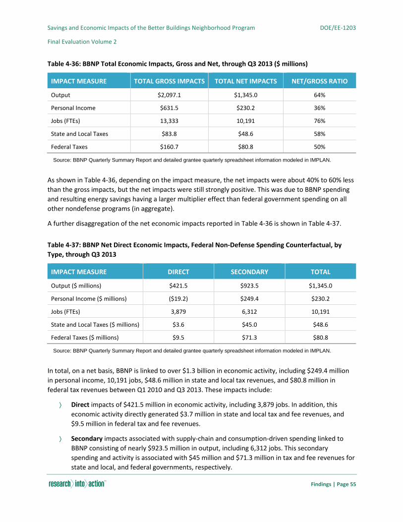
Savings and Economic Impacts of the Better Buildings Neighborhood Program DOE/EE-1203
Final Evaluation Volume 2
Findings | Page 55
Table 4-36: BBNP Total Economic Impacts, Gross and Net, through Q3 2013 ($ millions)
IMPACT MEASURE TOTAL GROSS IMPACTS TOTAL NET IMPACTS NET/GROSS RATIO
Output $2,097.1 $1,345.0 64%
Personal Income $631.5 $230.2 36%
Jobs (FTEs) 13,333 10,191 76%
State and Local Taxes $83.8 $48.6 58%
Federal Taxes $160.7 $80.8 50%
Source: BBNP Quarterly Summary Report and detailed grantee quarterly spreadsheet information modeled in IMPLAN.
As shown in Table 4-36, depending on the impact measure, the net impacts were about 40% to 60% less
than the gross impacts, but the net impacts were still strongly positive. This was due to BBNP spending
and resulting energy savings having a larger multiplier effect than federal government spending on all
other nondefense programs (in aggregate).
A further disaggregation of the net economic impacts reported in Table 4-36 is shown in Table 4-37.
Table 4-37: BBNP Net Direct Economic Impacts, Federal Non-Defense Spending Counterfactual, by
Type, through Q3 2013
IMPACT MEASURE DIRECT SECONDARY TOTAL
Output ($ millions) $421.5 $923.5 $1,345.0
Personal Income ($ millions) ($19.2) $249.4 $230.2
Jobs (FTEs) 3,879 6,312 10,191
State and Local Taxes ($ millions) $3.6 $45.0 $48.6
Federal Taxes ($ millions) $9.5 $71.3 $80.8
Source: BBNP Quarterly Summary Report and detailed grantee quarterly spreadsheet information modeled in IMPLAN.
In total, on a net basis, BBNP is linked to over $1.3 billion in economic activity, including $249.4 million
in personal income, 10,191 jobs, $48.6 million in state and local tax revenues, and $80.8 million in
federal tax revenues between Q1 2010 and Q3 2013. These impacts include:
Direct impacts of $421.5 million in economic activity, including 3,879 jobs. In addition, this
economic activity directly generated $3.7 million in state and local tax and fee revenues, and
$9.5 million in federal tax and fee revenues.
Secondary impacts associated with supply-chain and consumption-driven spending linked to
BBNP consisting of nearly $923.5 million in output, including 6,312 jobs. This secondary
spending and activity is associated with $45 million and $71.3 million in tax and fee revenues for
state and local, and federal governments, respectively.
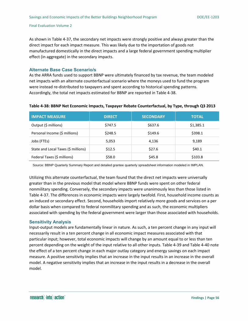
Savings and Economic Impacts of the Better Buildings Neighborhood Program DOE/EE-1203
Final Evaluation Volume 2
Findings | Page 56
As shown in Table 4-37, the secondary net impacts were strongly positive and always greater than the
direct impact for each impact measure. This was likely due to the importation of goods not
manufactured domestically in the direct impacts and a large federal government spending multiplier
effect (in aggregate) in the secondary impacts.
Alternate Base Case Scenario/s As the ARRA funds used to support BBNP were ultimately financed by tax revenue, the team modeled
net impacts with an alternate counterfactual scenario where the moneys used to fund the program
were instead re-distributed to taxpayers and spent according to historical spending patterns.
Accordingly, the total net impacts estimated for BBNP are reported in Table 4-38.
Table 4-38: BBNP Net Economic Impacts, Taxpayer Rebate Counterfactual, by Type, through Q3 2013
IMPACT MEASURE DIRECT SECONDARY TOTAL
Output ($ millions) $747.5 $637.6 $1,385.1
Personal Income ($ millions) $248.5 $149.6 $398.1
Jobs (FTEs) 5,053 4,136 9,189
State and Local Taxes ($ millions) $12.5 $27.6 $40.1
Federal Taxes ($ millions) $58.0 $45.8 $103.8
Source: BBNP Quarterly Summary Report and detailed grantee quarterly spreadsheet information modeled in IMPLAN.
Utilizing this alternate counterfactual, the team found that the direct net impacts were universally
greater than in the previous model that model where BBNP funds were spent on other federal
nonmilitary spending. Conversely, the secondary impacts were unanimously less than those listed in
Table 4-37. The differences in economic impacts were largely twofold. First, household income counts as
an induced or secondary effect. Second, households import relatively more goods and services on a per
dollar basis when compared to federal nonmilitary spending and as such, the economic multipliers
associated with spending by the federal government were larger than those associated with households.
Sensitivity Analysis
Input-output models are fundamentally linear in nature. As such, a ten percent change in any input will
necessarily result in a ten percent change in all economic impact measures associated with that
particular input; however, total economic impacts will change by an amount equal to or less than ten
percent depending on the weight of the input relative to all other inputs. Table 4-39 and Table 4-40 note
the effect of a ten percent change in each major outlay category and energy savings on each impact
measure. A positive sensitivity implies that an increase in the input results in an increase in the overall
model. A negative sensitivity implies that an increase in the input results in a decrease in the overall
model.
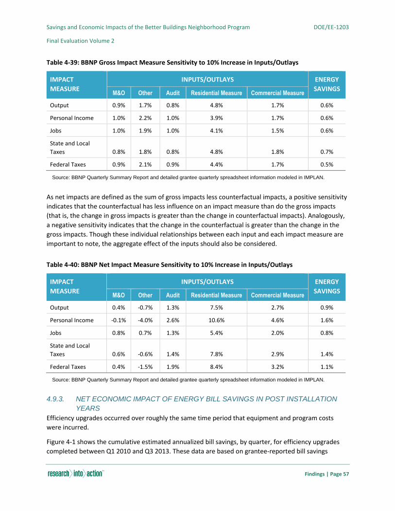
Savings and Economic Impacts of the Better Buildings Neighborhood Program DOE/EE-1203
Final Evaluation Volume 2
Findings | Page 57
Table 4-39: BBNP Gross Impact Measure Sensitivity to 10% Increase in Inputs/Outlays
IMPACT
MEASURE
INPUTS/OUTLAYS ENERGY
SAVINGS M&O Other Audit Residential Measure Commercial Measure
Output 0.9% 1.7% 0.8% 4.8% 1.7% 0.6%
Personal Income 1.0% 2.2% 1.0% 3.9% 1.7% 0.6%
Jobs 1.0% 1.9% 1.0% 4.1% 1.5% 0.6%
State and Local
Taxes 0.8% 1.8% 0.8% 4.8% 1.8% 0.7%
Federal Taxes 0.9% 2.1% 0.9% 4.4% 1.7% 0.5%
Source: BBNP Quarterly Summary Report and detailed grantee quarterly spreadsheet information modeled in IMPLAN.
As net impacts are defined as the sum of gross impacts less counterfactual impacts, a positive sensitivity
indicates that the counterfactual has less influence on an impact measure than do the gross impacts
(that is, the change in gross impacts is greater than the change in counterfactual impacts). Analogously,
a negative sensitivity indicates that the change in the counterfactual is greater than the change in the
gross impacts. Though these individual relationships between each input and each impact measure are
important to note, the aggregate effect of the inputs should also be considered.
Table 4-40: BBNP Net Impact Measure Sensitivity to 10% Increase in Inputs/Outlays
IMPACT
MEASURE
INPUTS/OUTLAYS ENERGY
SAVINGS M&O Other Audit Residential Measure Commercial Measure
Output 0.4% -0.7% 1.3% 7.5% 2.7% 0.9%
Personal Income -0.1% -4.0% 2.6% 10.6% 4.6% 1.6%
Jobs 0.8% 0.7% 1.3% 5.4% 2.0% 0.8%
State and Local
Taxes 0.6% -0.6% 1.4% 7.8% 2.9% 1.4%
Federal Taxes 0.4% -1.5% 1.9% 8.4% 3.2% 1.1%
Source: BBNP Quarterly Summary Report and detailed grantee quarterly spreadsheet information modeled in IMPLAN.
4.9.3. NET ECONOMIC IMPACT OF ENERGY BILL SAVINGS IN POST INSTALLATION
YEARS
Efficiency upgrades occurred over roughly the same time period that equipment and program costs
were incurred.
Figure 4-1 shows the cumulative estimated annualized bill savings, by quarter, for efficiency upgrades
completed between Q1 2010 and Q3 2013. These data are based on grantee-reported bill savings
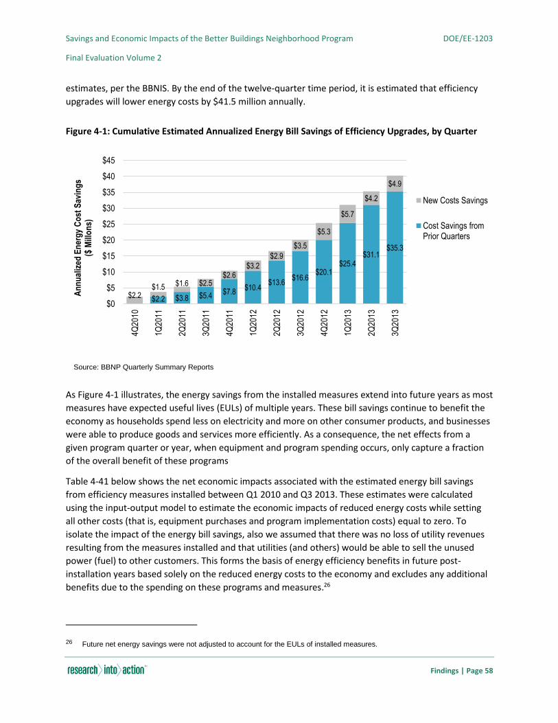
Savings and Economic Impacts of the Better Buildings Neighborhood Program DOE/EE-1203
Final Evaluation Volume 2
Findings | Page 58
estimates, per the BBNIS. By the end of the twelve-quarter time period, it is estimated that efficiency
upgrades will lower energy costs by $41.5 million annually.
Figure 4-1: Cumulative Estimated Annualized Energy Bill Savings of Efficiency Upgrades, by Quarter
Source: BBNP Quarterly Summary Reports
As Figure 4-1 illustrates, the energy savings from the installed measures extend into future years as most
measures have expected useful lives (EULs) of multiple years. These bill savings continue to benefit the
economy as households spend less on electricity and more on other consumer products, and businesses
were able to produce goods and services more efficiently. As a consequence, the net effects from a
given program quarter or year, when equipment and program spending occurs, only capture a fraction
of the overall benefit of these programs
Table 4-41 below shows the net economic impacts associated with the estimated energy bill savings
from efficiency measures installed between Q1 2010 and Q3 2013. These estimates were calculated
using the input-output model to estimate the economic impacts of reduced energy costs while setting
all other costs (that is, equipment purchases and program implementation costs) equal to zero. To
isolate the impact of the energy bill savings, also we assumed that there was no loss of utility revenues
resulting from the measures installed and that utilities (and others) would be able to sell the unused
power (fuel) to other customers. This forms the basis of energy efficiency benefits in future post-
installation years based solely on the reduced energy costs to the economy and excludes any additional
benefits due to the spending on these programs and measures.26
26 Future net energy savings were not adjusted to account for the EULs of installed measures.
$2.2 $3.8 $5.4$7.8
$10.4$13.6
$16.6$20.1
$25.4$31.1
$35.3
$2.2$1.5 $1.6 $2.5
$2.6$3.2
$2.9
$3.5
$5.3
$5.7
$4.2
$4.9
$0
$5
$10
$15
$20
$25
$30
$35
$40
$45
4Q20
10
1Q20
11
2Q20
11
3Q20
11
4Q20
11
1Q20
12
2Q20
12
3Q20
12
4Q20
12
1Q20
13
2Q20
13
3Q20
13
An
nu
aliz
ed E
ner
gy
Co
st S
avin
gs
($ M
illo
ns)
New Costs Savings
Cost Savings fromPrior Quarters
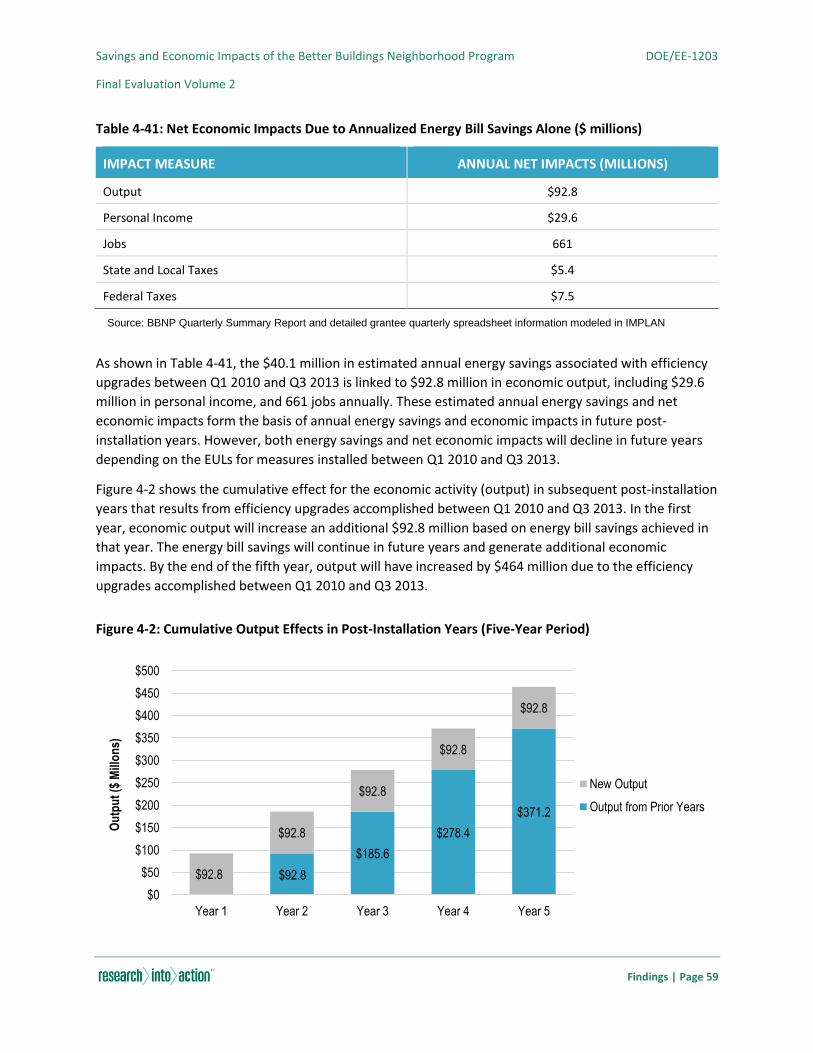
Savings and Economic Impacts of the Better Buildings Neighborhood Program DOE/EE-1203
Final Evaluation Volume 2
Findings | Page 59
Table 4-41: Net Economic Impacts Due to Annualized Energy Bill Savings Alone ($ millions)
IMPACT MEASURE ANNUAL NET IMPACTS (MILLIONS)
Output $92.8
Personal Income $29.6
Jobs 661
State and Local Taxes $5.4
Federal Taxes $7.5
Source: BBNP Quarterly Summary Report and detailed grantee quarterly spreadsheet information modeled in IMPLAN
As shown in Table 4-41, the $40.1 million in estimated annual energy savings associated with efficiency
upgrades between Q1 2010 and Q3 2013 is linked to $92.8 million in economic output, including $29.6
million in personal income, and 661 jobs annually. These estimated annual energy savings and net
economic impacts form the basis of annual energy savings and economic impacts in future post-
installation years. However, both energy savings and net economic impacts will decline in future years
depending on the EULs for measures installed between Q1 2010 and Q3 2013.
Figure 4-2 shows the cumulative effect for the economic activity (output) in subsequent post-installation
years that results from efficiency upgrades accomplished between Q1 2010 and Q3 2013. In the first
year, economic output will increase an additional $92.8 million based on energy bill savings achieved in
that year. The energy bill savings will continue in future years and generate additional economic
impacts. By the end of the fifth year, output will have increased by $464 million due to the efficiency
upgrades accomplished between Q1 2010 and Q3 2013.
Figure 4-2: Cumulative Output Effects in Post-Installation Years (Five-Year Period)
$92.8
$185.6
$278.4
$371.2
$92.8
$92.8
$92.8
$92.8
$92.8
$0
$50
$100
$150
$200
$250
$300
$350
$400
$450
$500
Year 1 Year 2 Year 3 Year 4 Year 5
Ou
tpu
t ($
Mill
on
s)
New Output
Output from Prior Years
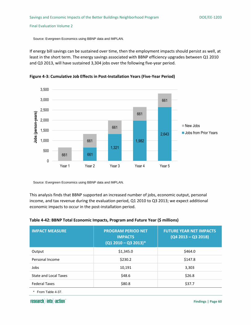
Savings and Economic Impacts of the Better Buildings Neighborhood Program DOE/EE-1203
Final Evaluation Volume 2
Findings | Page 60
Source: Evergreen Economics using BBNP data and IMPLAN.
If energy bill savings can be sustained over time, then the employment impacts should persist as well, at
least in the short term. The energy savings associated with BBNP efficiency upgrades between Q1 2010
and Q3 2013, will have sustained 3,304 jobs over the following five-year period.
Figure 4-3: Cumulative Job Effects in Post-Installation Years (Five-Year Period)
Source: Evergreen Economics using BBNP data and IMPLAN.
This analysis finds that BBNP supported an increased number of jobs, economic output, personal
income, and tax revenue during the evaluation period, Q1 2010 to Q3 2013; we expect additional
economic impacts to occur in the post-installation period.
Table 4-42: BBNP Total Economic Impacts, Program and Future Year ($ millions)
IMPACT MEASURE PROGRAM PERIOD NET
IMPACTS
(Q1 2010 – Q3 2013)*
FUTURE YEAR NET IMPACTS
(Q4 2013 – Q3 2018)
Output $1,345.0 $464.0
Personal Income $230.2 $147.8
Jobs 10,191 3,303
State and Local Taxes $48.6 $26.8
Federal Taxes $80.8 $37.7
* From Table 4-37.
661
1,321
1,982
2,643
661
661
661
661
661
0
500
1,000
1,500
2,000
2,500
3,000
3,500
Year 1 Year 2 Year 3 Year 4 Year 5
Job
s (p
erso
n-y
ears
)
New Jobs
Jobs from Prior Years
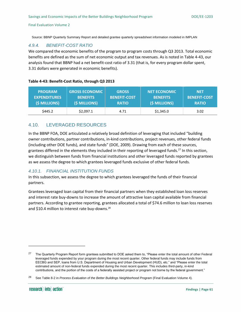
Savings and Economic Impacts of the Better Buildings Neighborhood Program DOE/EE-1203
Final Evaluation Volume 2
Findings | Page 61
Source: BBNP Quarterly Summary Report and detailed grantee quarterly spreadsheet information modeled in IMPLAN
4.9.4. BENEFIT-COST RATIO
We compared the economic benefits of the program to program costs through Q3 2013. Total economic
benefits are defined as the sum of net economic output and tax revenues. As is noted in Table 4-43, our
analysis found that BBNP had a net benefit-cost ratio of 3.31 (that is, for every program dollar spent,
3.31 dollars were generated in economic benefits).
Table 4-43: Benefit-Cost Ratio, through Q3 2013
PROGRAM
EXPENDITURES
($ MILLIONS)
GROSS ECONOMIC
BENEFITS
($ MILLIONS)
GROSS
BENEFIT-COST
RATIO
NET ECONOMIC
BENEFITS
($ MILLIONS)
NET
BENEFIT-COST
RATIO
$445.2 $2,097.1 4.71 $1,345.0 3.02
4.10. LEVERAGED RESOURCES
In the BBNP FOA, DOE articulated a relatively broad definition of leveraging that included “building
owner contributions, partner contributions, in-kind contributions, project revenues, other federal funds
(including other DOE funds), and state funds” (DOE, 2009). Drawing from each of these sources,
grantees differed in the elements they included in their reporting of leveraged funds.27 In this section,
we distinguish between funds from financial institutions and other leveraged funds reported by grantees
as we assess the degree to which grantees leveraged funds exclusive of other federal funds.
4.10.1. FINANCIAL INSTITUTION FUNDS
In this subsection, we assess the degree to which grantees leveraged the funds of their financial
partners.
Grantees leveraged loan capital from their financial partners when they established loan loss reserves
and interest rate buy-downs to increase the amount of attractive loan capital available from financial
partners. According to grantee reporting, grantees allocated a total of $74.6 million to loan loss reserves
and $10.4 million to interest rate buy-downs.28
27 The Quarterly Program Report form grantees submitted to DOE asked them to, “Please enter the total amount of other Federal
leveraged funds expended by your program during the most recent quarter. Other federal funds may include funds from
EECBG and SEP, loans from U.S. Department of Housing and Urban Development (HUD), etc.” and “Please enter the total
estimated amount of non-federal funds expended during the most recent quarter. This includes third-party, in-kind
contributions, and the portion of the costs of a federally assisted project or program not borne by the federal government.”
28 See Table 8-2 in Process Evaluation of the Better Buildings Neighborhood Program (Final Evaluation Volume 4).

Savings and Economic Impacts of the Better Buildings Neighborhood Program DOE/EE-1203
Final Evaluation Volume 2
Findings | Page 62
Table 4-44: Types of Financing Support Grantees Provided
TYPE OF FINANCING SUPPORT SECTOR NUMBER OF
GRANTEES
PROVIDING
TOTAL SPENDING
Loan Loss Reserve Commercial (n = 19) 13 $36,704,152
Residential (n = 30) 17 $30,154,770
Multi-sector 3 $7,790,688
Total (n = 36) 27 $74,649,610
Revolving Loan Fund Commercial (n = 19) 13 $39,180,788
Residential (n = 30) 16 $28,554,673
Total (n = 36) 22 $67,735,461
Interest Rate Buy Down Total (n = 36) 15* $10,399,460
* Reported data did not differentiate interest rate buy down spending by sector.
Source: Process Evaluation of the Better Buildings Neighborhood Program (Final Evaluation Volume 4), Table 8-2.
Grantees further reported they leveraged financial loan funds of about $618 million. Our interviews with
contacts at partnering financial institutions corroborate this figure as a lower-bound estimate of
leveraged financial institution funds.29
We found a number of occurrences of missing data in the grantees’ reports of leverage financial
resources (that is, missing data for grantees also reporting they had established loan loss reserves and
interest rate buy-downs). Thus, we conducted the following analysis to estimate an upper-bound
estimate of leveraged financial institution funds.
Grantees using loan loss reserves most often placed 5% or 10% of each loan in reserve, making between
10 and 20 times the value of the grantee’s contribution available for program lending.30 A loan loss
reserve likely leveraged approximately five times the grantee’s contribution in loan capital.31 Assuming
grantees leveraged ten times their spending on loan loss reserves and five times their spending on
29 Chapter 8 of Volume 4 presents the findings of these interviews. The interview data provide support for the reported amounts;
the interview data are insufficient to confirm or verify the amounts.
30 Each $1 placed in a reserve fund with a coverage ratio of 5%, would support $20 of lending; each $1 placed in a reserve fund
of 10% would support $10 of lending. Concepts adapted from Zimring 2014. Data on amounts grantees placed in loan loss
reserves from grantee interviews.
31 For example, the difference in interest a financial institution would receive on a 10-year, $10,000 loan at 2% interest as
opposed to 7% interest is approximately $2,900. Grantees may not have compensated financial institutions for this full value to
account for the benefit to the financial institution of receiving the interest income as a lump sum.

Savings and Economic Impacts of the Better Buildings Neighborhood Program DOE/EE-1203
Final Evaluation Volume 2
Findings | Page 63
interest rate buy-downs, grantees leveraged up to approximately $800 million in lending capacity.32 This
is an upper-bound estimate, since some grantees used both loan loss reserves and interest rate buy-
downs on the same pools of loan capital.
4.10.2. OTHER LEVERAGED FUNDS
In this subsection, we assess the degree to which grantees leveraged funds from other sources (federal
and non-federal exclusive of financial institution partners).
Table 4-46 summarizes all the leveraged funds – both federal and non-federal – that grantees reported
to DOE, as recorded in the BBNIS. Over the grant period, grantees reported spending more than $98
million in federal funds excluding their BBNP grants, as well as $655 million in non-federal funds (shown
subsequently in Table 4-46), for a total of about $753 million.33
Table 4-45: Reported Leveraged Funds (Federal and Non-federal)
TOTAL AVERAGE TOTAL
Total $28,370,016 $753,170,655
Small Award Grantees ($5M or less) $3,352,071 $67,041,415
Medium Award Grantees (more than $5M to less than $20M) $20,425,073 $265,525,952
Large Award Grantees ($20M or more) $52,575,411 $420,603,287
Source: Research Into Action, analysis of BBNIS data.
We did not explore with grantees who provided these reported total funds and how the funds were
used. However, we explored these questions for a subset of the reported funds that appeared to satisfy
Wolf’s definition of leveraging.34 Our estimates on non-federal leveraged funds from this research
therefore represent a lower bound of other leveraged funds.
As described in Section 3.6.4, we interviewed the 15 grantees reporting the largest quantities of non-
federal leveraged funds – $546 million in total – an amount equal to 83% of the $655 million in
leveraged funds reported by all grantees. Table 4-45 provides the non-federal leveraged funds reported
by the interviewed grantees ($546 million) and the spending of leveraged funds we estimated for these
15 grantees using the Wolf method - $16 million. For nearly half (7 of 16) of the interviewed grantees,
we could not identify any funds that met Wolf’s leverage definition.35 The table extrapolates from the
32 DOE did not request grantees to report funds leveraged from financial institutions, thus we estimated the amount of leveraged
funds using the approach described.
33 The data describe program expenditures by any party – the grantee or its partners.
34 See Appendix B-11.
35 Since this assessment began, EERE has initiated a project with the aim of operationalizing a calculation tool for the consistent
estimation of leveraged resources across EERE programs. Originally intended to follow the strict definition postulated by Wolf,
early implementation activities, involving in-depth interviews with additional stakeholders (including the authors of this report)
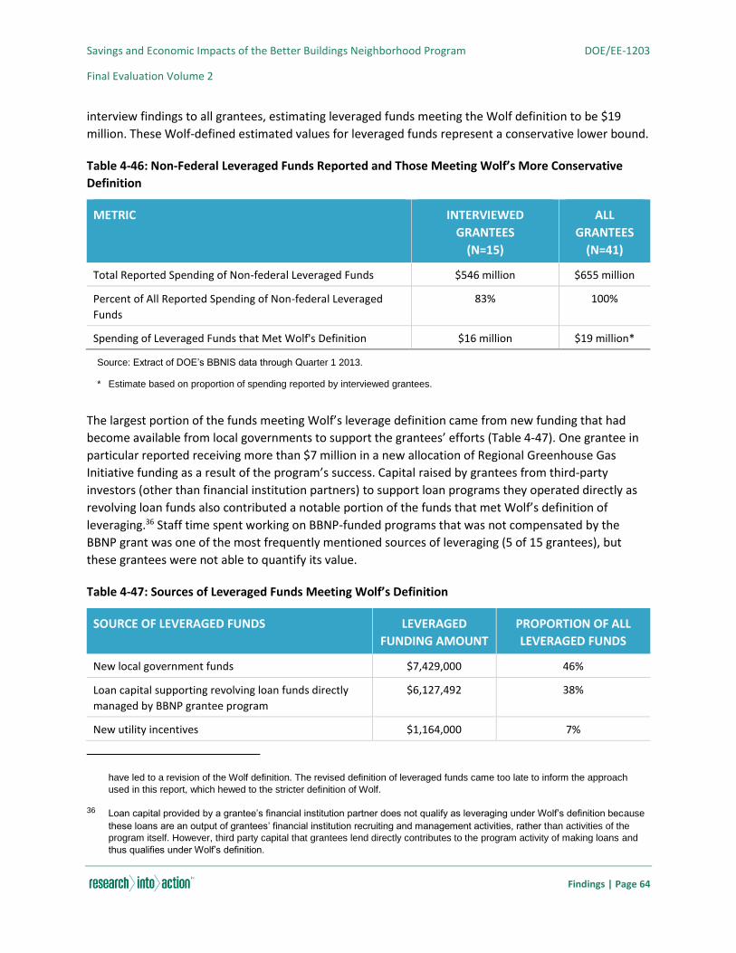
Savings and Economic Impacts of the Better Buildings Neighborhood Program DOE/EE-1203
Final Evaluation Volume 2
Findings | Page 64
interview findings to all grantees, estimating leveraged funds meeting the Wolf definition to be $19
million. These Wolf-defined estimated values for leveraged funds represent a conservative lower bound.
Table 4-46: Non-Federal Leveraged Funds Reported and Those Meeting Wolf’s More Conservative
Definition
METRIC INTERVIEWED
GRANTEES
(N=15)
ALL
GRANTEES
(N=41)
Total Reported Spending of Non-federal Leveraged Funds $546 million $655 million
Percent of All Reported Spending of Non-federal Leveraged
Funds
83% 100%
Spending of Leveraged Funds that Met Wolf's Definition $16 million $19 million*
Source: Extract of DOE’s BBNIS data through Quarter 1 2013.
* Estimate based on proportion of spending reported by interviewed grantees.
The largest portion of the funds meeting Wolf’s leverage definition came from new funding that had
become available from local governments to support the grantees’ efforts (Table 4-47). One grantee in
particular reported receiving more than $7 million in a new allocation of Regional Greenhouse Gas
Initiative funding as a result of the program’s success. Capital raised by grantees from third-party
investors (other than financial institution partners) to support loan programs they operated directly as
revolving loan funds also contributed a notable portion of the funds that met Wolf’s definition of
leveraging.36 Staff time spent working on BBNP-funded programs that was not compensated by the
BBNP grant was one of the most frequently mentioned sources of leveraging (5 of 15 grantees), but
these grantees were not able to quantify its value.
Table 4-47: Sources of Leveraged Funds Meeting Wolf’s Definition
SOURCE OF LEVERAGED FUNDS LEVERAGED
FUNDING AMOUNT
PROPORTION OF ALL
LEVERAGED FUNDS
New local government funds $7,429,000 46%
Loan capital supporting revolving loan funds directly
managed by BBNP grantee program
$6,127,492 38%
New utility incentives $1,164,000 7%
have led to a revision of the Wolf definition. The revised definition of leveraged funds came too late to inform the approach
used in this report, which hewed to the stricter definition of Wolf.
36 Loan capital provided by a grantee’s financial institution partner does not qualify as leveraging under Wolf’s definition because
these loans are an output of grantees’ financial institution recruiting and management activities, rather than activities of the
program itself. However, third party capital that grantees lend directly contributes to the program activity of making loans and
thus qualifies under Wolf’s definition.
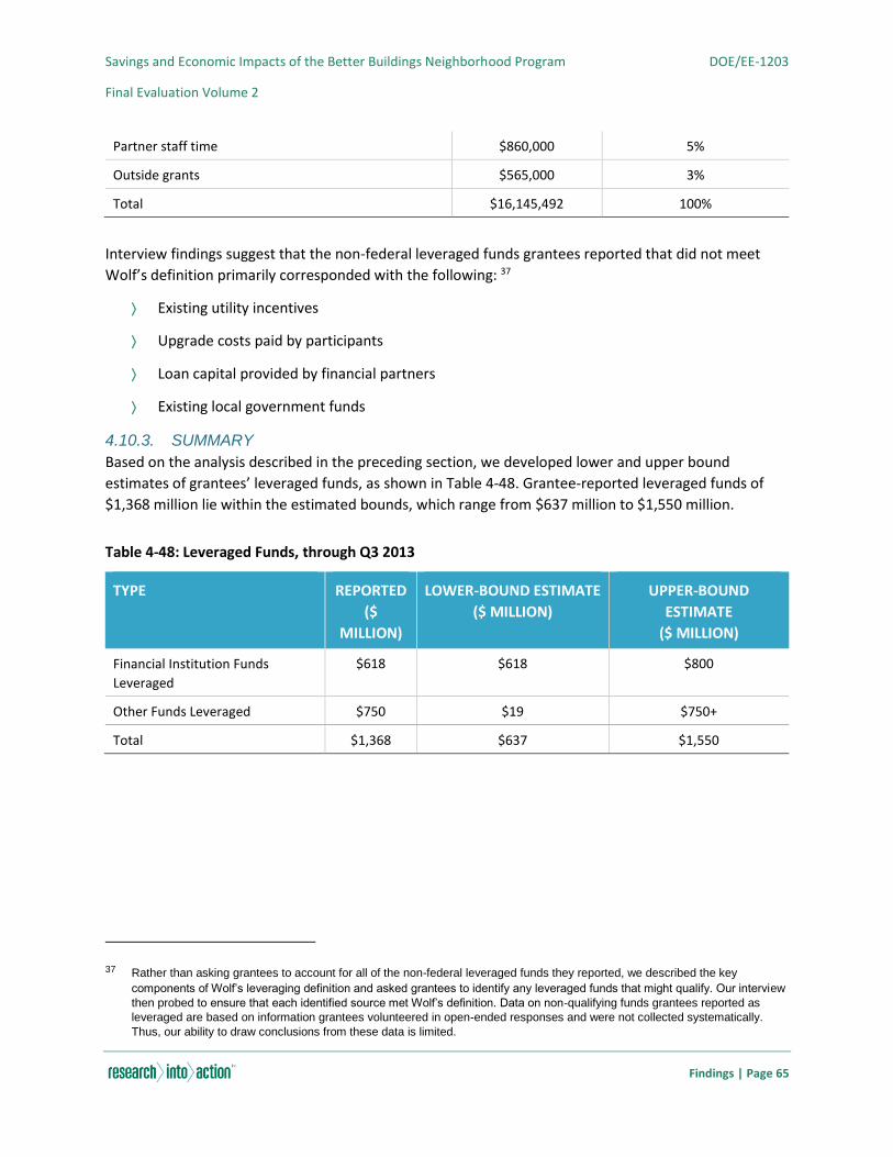
Savings and Economic Impacts of the Better Buildings Neighborhood Program DOE/EE-1203
Final Evaluation Volume 2
Findings | Page 65
Partner staff time $860,000 5%
Outside grants $565,000 3%
Total $16,145,492 100%
Interview findings suggest that the non-federal leveraged funds grantees reported that did not meet
Wolf’s definition primarily corresponded with the following: 37
Existing utility incentives
Upgrade costs paid by participants
Loan capital provided by financial partners
Existing local government funds
4.10.3. SUMMARY
Based on the analysis described in the preceding section, we developed lower and upper bound
estimates of grantees’ leveraged funds, as shown in Table 4-48. Grantee-reported leveraged funds of
$1,368 million lie within the estimated bounds, which range from $637 million to $1,550 million.
Table 4-48: Leveraged Funds, through Q3 2013
TYPE REPORTED
($
MILLION)
LOWER-BOUND ESTIMATE
($ MILLION)
UPPER-BOUND
ESTIMATE
($ MILLION)
Financial Institution Funds
Leveraged
$618 $618 $800
Other Funds Leveraged $750 $19 $750+
Total $1,368 $637 $1,550
37 Rather than asking grantees to account for all of the non-federal leveraged funds they reported, we described the key
components of Wolf’s leveraging definition and asked grantees to identify any leveraged funds that might qualify. Our interview
then probed to ensure that each identified source met Wolf’s definition. Data on non-qualifying funds grantees reported as
leveraged are based on information grantees volunteered in open-ended responses and were not collected systematically.
Thus, our ability to draw conclusions from these data is limited.

Savings and Economic Impacts of the Better Buildings Neighborhood Program DOE/EE-1203
Final Evaluation Volume 2
Lessons Learned, Conclusions, and Recommendations | Page 66
5. LESSONS LEARNED, CONCLUSIONS, AND RECOMMENDATIONS
The chapter provides the lessons learned as part of the preliminary and final evaluation activities, our
conclusions, and our recommendations for improving future design, implementation, and evaluations of
similar programs.
5.1. LESSONS LEARNED
We believe the final impact evaluation was an overall success, and many lessons were learned along the
way. As discussed, we faced multiple challenges during both the planning and implementation of the
impact evaluation. While navigating these challenges, we identified lessons learned that will help shape
the future of similar program evaluations. We offer the following lessons, organized as lessons learned
during interactions with grantees, learned during sampling execution, and learned during the overall
evaluation activities.
5.1.1. GRANTEE INTERACTION
We had multiple and varied interactions with each grantee, including interviews, data requests, and
discussions to augment our understanding of their program offerings and structure. We draw several
lessons from these interactions.
Allow sufficient time to request and gather data from the Grantees. We made data requests to
almost 30 grantees for the preliminary evaluation. This process to submit requests and receive
data required four months to complete. This timeframe was reduced during the final evaluation
process, as grantees understood our needs and the format of the data required. Regardless,
future evaluations should understand that grantees are busy and, unlike most utility companies,
they are not equipped with the tools and databases to easily extract participant and project-
level information. It is necessary to give them sufficient time to gather requested data.
Give clear and concise data requests. Grantees are busy and frequently understaffed. In
addition, many of these grantees have little experience with evaluations. Making clear and
concise data requests that include specific information required by the team for analysis
(including invoices, audit reports, project applications, etc.) help to speed up the response time
and alleviate any concerns or questions that they may have regarding data needs.
Know when to stop asking. When requesting data from multiple grantees, many of whom are
not already experienced in the area of program evaluation, it is necessary to be patient yet
persuasive regarding the importance of the data requests. It also is necessary to know when to
stop asking for more data and move forward with what has been provided.
5.1.2. SAMPLING
The sampling strategy contributes substantially to the accuracy and usefulness of the impact evaluation
results. The following lessons summarize our experience.
Use proper sampling techniques. When seeking to examine savings across multiple and diverse
programs such as those offered through BBNP, the team needed to examine the effectiveness of

Savings and Economic Impacts of the Better Buildings Neighborhood Program DOE/EE-1203
Final Evaluation Volume 2
Lessons Learned, Conclusions, and Recommendations | Page 67
the sampling and the level of rigor employed on the sample. Budget and time constraints put
limits on the ability to sample at a high level of rigor across all the grantees. The team designed
the sampling strategy with the knowledge that the programs were very diverse and that the
reporting procedures were varied and not always consistent. Therefore, the sampling
parameters that were used to determine the sample sizes took this known uncertainty and
potential range of error into account.
Be flexible. The initial sampling strategy was informed by preliminary grantee interviews and
the review of available data at a certain point in time. After the team fully analyzed the data that
were provided by the grantees, changes were made in the sampling design and approach.
Additionally, grantees provided periodic project updates which adjusted savings and project
counts throughout the evaluation activities. The team had to analyze these adjustments to
determine the impact on the validity of the sample.
5.1.3. EVALUATION ACTIVITIES
We utilized several levels of rigor when determining gross verified savings. We typically followed
standard practices as seen in most utility-funded evaluation activities, but found that approaches that
may work for a utility-funded program may not necessarily be as successful for a program with the large
scale, scope, and diversity of BBNP.
Phone verifications had limited value. Phone verifications are standard practice in many utility-
funded impact evaluations. While the phone surveys were useful in verifying overall project
participation and obtaining information on program influence, we determined during the
preliminary evaluation that the phone verifications used for M&V often provided limited value.
The majority of participants interviewed had difficulty remembering the specifics surrounding
completed upgrades, and gathering key data on measures implemented. This was likely due to
the long timespan (averaging one to two years) between measure installation and phone
verifications. There also was confusion among participants regarding the measure funding
source (BBNP or local utility program).
Onsite verifications were valuable. While the phone surveys proved challenging, the onsite
surveys were valuable in obtaining a greater level of detail regarding project implementation
than could be obtained during phone verifications. We do note that onsite verification also has
limitations such as the inability to confirm baseline equipment or restricted access to upgraded
measures (for example, insulation). However, for the purposes of the BBNP evaluation, we
found the onsite data to be more reliable and useful than the phone survey data.
Reasons for variances in the data were multifaceted. There was no one reason for the
discrepancies between the reporting databases used by the grantees and DOE. Both parties
were faced with multiple challenges while attempting to develop accurate reports of program
progress. We interacted frequently with DOE and the grantees to understand the underlying
issues effecting the data.
5.1.4. REPORTING INFRASTRUCTURE
DOE funded BBNP with the objective of creating jobs, saving energy, and setting the foundation for
future similar programs. It is difficult for a program of this breadth and depth to create a centralized,

Savings and Economic Impacts of the Better Buildings Neighborhood Program DOE/EE-1203
Final Evaluation Volume 2
Lessons Learned, Conclusions, and Recommendations | Page 68
consistent, and easy-to-use system for individual program tracking and reporting. However, one key
lesson learned as a result of this evaluation is the importance of the design and enforcement of proper
reporting processes. The design of proper reporting processes and concise yet all-inclusive data
capturing procedures is crucial to the success of any program of this scale and magnitude. In addition,
this lesson can be carried into energy efficiency program design, both for utility-funded structures and
for nonutility structures, such as those that exist in BBNP. Designing a reporting structure that captures
the basic data effectively and accurately is essential to a successful program both in the near term and
the long term. Clear reporting procedures lead to a better understanding of the program effects both in
the context of energy savings and the proper use of resources. This, in turn, helps lead to better
program design in the future and greater program success. Additionally, some level of enforcement
regarding the proper reporting would encourage accountability.
5.2. CONCLUSIONS
5.2.1. GOAL AND OBJECTIVE ATTAINMENT
By the end of the three-year evaluation period (Q4 2010 to Q3 2013), BBNP had met the three ARRA
goals, as shown in Table 5-1. The table presents, among other findings, our findings of net jobs, net
economic activity, and net benefit-cost ratio. For the economic metrics, the term “net” signifies BBNP’s
contribution to these outcomes above and beyond the outcomes that would have occurred had the
BBNP funding been spent according to historical non-defense federal spending patterns.
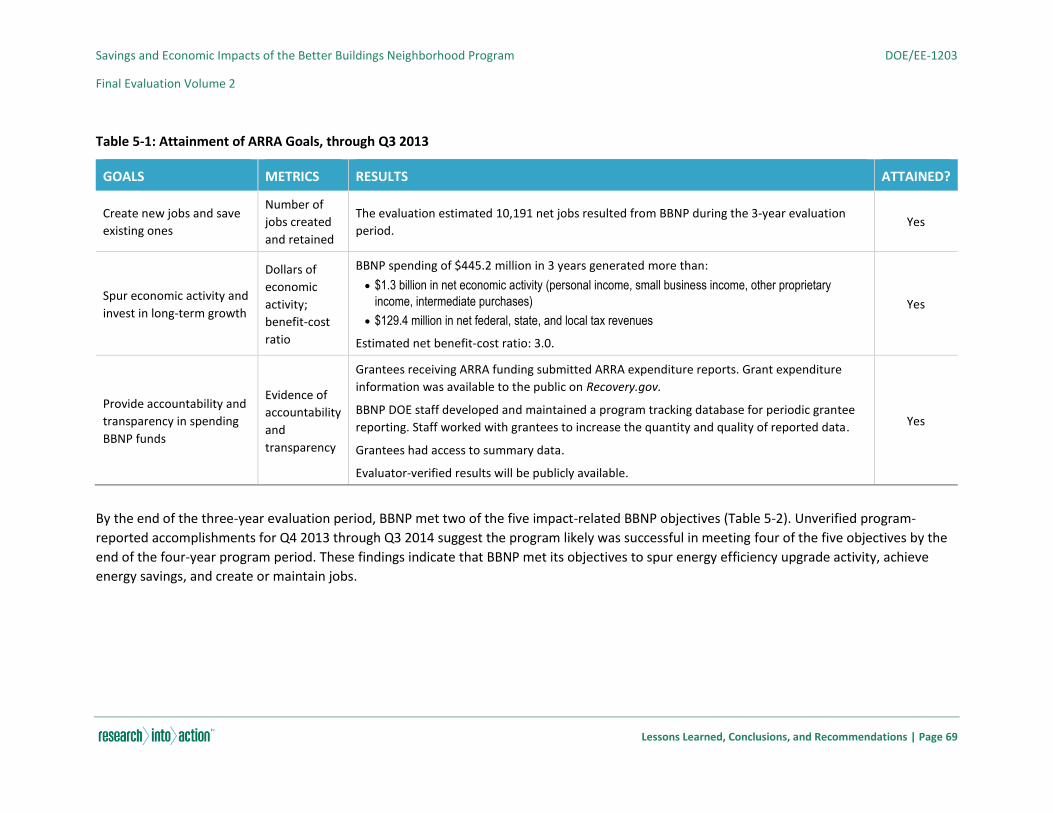
Savings and Economic Impacts of the Better Buildings Neighborhood Program DOE/EE-1203
Final Evaluation Volume 2
Lessons Learned, Conclusions, and Recommendations | Page 69
Table 5-1: Attainment of ARRA Goals, through Q3 2013
GOALS METRICS RESULTS ATTAINED?
Create new jobs and save
existing ones
Number of
jobs created
and retained
The evaluation estimated 10,191 net jobs resulted from BBNP during the 3-year evaluation
period. Yes
Spur economic activity and
invest in long-term growth
Dollars of
economic
activity;
benefit-cost
ratio
BBNP spending of $445.2 million in 3 years generated more than:
$1.3 billion in net economic activity (personal income, small business income, other proprietary
income, intermediate purchases)
$129.4 million in net federal, state, and local tax revenues
Estimated net benefit-cost ratio: 3.0.
Yes
Provide accountability and
transparency in spending
BBNP funds
Evidence of
accountability
and
transparency
Grantees receiving ARRA funding submitted ARRA expenditure reports. Grant expenditure
information was available to the public on Recovery.gov.
BBNP DOE staff developed and maintained a program tracking database for periodic grantee
reporting. Staff worked with grantees to increase the quantity and quality of reported data.
Grantees had access to summary data.
Evaluator-verified results will be publicly available.
Yes
By the end of the three-year evaluation period, BBNP met two of the five impact-related BBNP objectives (Table 5-2). Unverified program-
reported accomplishments for Q4 2013 through Q3 2014 suggest the program likely was successful in meeting four of the five objectives by the
end of the four-year program period. These findings indicate that BBNP met its objectives to spur energy efficiency upgrade activity, achieve
energy savings, and create or maintain jobs.
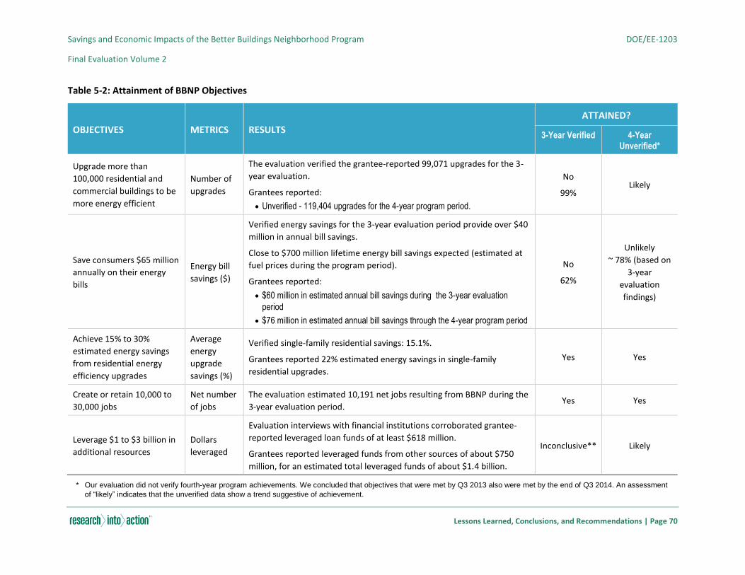
Savings and Economic Impacts of the Better Buildings Neighborhood Program DOE/EE-1203
Final Evaluation Volume 2
Lessons Learned, Conclusions, and Recommendations | Page 70
Table 5-2: Attainment of BBNP Objectives
OBJECTIVES METRICS RESULTS
ATTAINED?
3-Year Verified 4-Year Unverified*
Upgrade more than
100,000 residential and
commercial buildings to be
more energy efficient
Number of
upgrades
The evaluation verified the grantee-reported 99,071 upgrades for the 3-
year evaluation.
Grantees reported:
Unverified - 119,404 upgrades for the 4-year program period.
No
99% Likely
Save consumers $65 million
annually on their energy
bills
Energy bill
savings ($)
Verified energy savings for the 3-year evaluation period provide over $40
million in annual bill savings.
Close to $700 million lifetime energy bill savings expected (estimated at
fuel prices during the program period).
Grantees reported:
$60 million in estimated annual bill savings during the 3-year evaluation
period
$76 million in estimated annual bill savings through the 4-year program period
No
62%
Unlikely
~ 78% (based on
3-year
evaluation
findings)
Achieve 15% to 30%
estimated energy savings
from residential energy
efficiency upgrades
Average
energy
upgrade
savings (%)
Verified single-family residential savings: 15.1%.
Grantees reported 22% estimated energy savings in single-family
residential upgrades.
Yes Yes
Create or retain 10,000 to
30,000 jobs
Net number
of jobs
The evaluation estimated 10,191 net jobs resulting from BBNP during the
3-year evaluation period. Yes Yes
Leverage $1 to $3 billion in
additional resources
Dollars
leveraged
Evaluation interviews with financial institutions corroborated grantee-
reported leveraged loan funds of at least $618 million.
Grantees reported leveraged funds from other sources of about $750
million, for an estimated total leveraged funds of about $1.4 billion.
Inconclusive** Likely
* Our evaluation did not verify fourth-year program achievements. We concluded that objectives that were met by Q3 2013 also were met by the end of Q3 2014. An assessment
of “likely” indicates that the unverified data show a trend suggestive of achievement.

Savings and Economic Impacts of the Better Buildings Neighborhood Program DOE/EE-1203
Final Evaluation Volume 2
Lessons Learned, Conclusions, and Recommendations | Page 71
** The evaluation addressed financial leverage amounts only; it did not address other grantee-reported leveraged funds. See Leveraged Resources for more information.

Savings and Economic Impacts of the Better Buildings Neighborhood Program DOE/EE-1203
Final Evaluation Volume 2
Lessons Learned, Conclusions, and Recommendations | Page 72
5.2.2. IMPACT ASSESSMENT LESSONS LEARNED
The main objective of this impact evaluation was to determine the impacts of $508 million in BBNP
spending that allocated resources to varied energy efficiency programs across the country. The
challenges associated with this task, such as difficulty in acquiring grantee data, lack of quality
control/assurance leading to inaccuracies of reported metrics, and the large scale and broad scope of
grantee programs, affected the team’s evaluation activities. While navigating these challenges, we
learned many lessons that will help shape the future of similar program evaluations. Key among these
lessons are:
Allow sufficient time to request and gather data from the grantees. Grantees are busy, and
unlike most utility-funded efficiency program managers, they are not equipped with the tools
and databases to easily extract participant and project level information. In addition, grantees
are frequently understaffed, so making clear and concise data requests are necessary to help
speed up the response time and alleviate any concerns or questions that they may have
regarding data needs.
Phone verifications had limited value. Phone verifications are standard practice in many utility-
funded impact evaluations. While the phone surveys were useful in verifying overall project
participation and obtaining information on program influence, we determined during the
preliminary evaluation that the phone verifications used for M&V often provided limited value.
The majority of participants interviewed had difficulty remembering the specifics surrounding
completed upgrades, and gathering key data on measures implemented. This is likely due to the
long timespan (averaging one to two years) between measure installation and phone
verifications. There also was confusion among participants regarding the measure funding
source (BBNP or local utility program).
Onsite verifications were valuable. While onsite surveys encounter some of the same issues
with reliability as the phone surveys, the onsite surveys were valuable in obtaining a greater
level of detail regarding project implementation than could be obtained during phone
verifications and file review.
5.3. RECOMMENDATIONS
The grant cycle for BBNP has ended, and it is unclear whether or not, in the foreseeable future, DOE will
fund a program on a scale similar to BBNP. Were DOE or another agency to fund a program like BBNP,
we offer the following recommendations to foster greater consistency in program expectations, design,
tracking, and reporting:
Plan and develop a comprehensive and easy to use data tracking and reporting system
available to grantees at time of funding award. Due to the size of the funding pool and the
speed at which it needed to be issued, there was a limited focus on program evaluation and
reporting needs when BBNP was designed and launched. The resulting tracking and reporting
processes were cumbersome, inconsistent, and frustrating for both grantees and DOE. It is
critical that for any future programs, consideration be given to the data tracking and reporting

Savings and Economic Impacts of the Better Buildings Neighborhood Program DOE/EE-1203
Final Evaluation Volume 2
Lessons Learned, Conclusions, and Recommendations | Page 73
needs for both a successful and streamlined program, but also for the needs of data verification
and program evaluation.
Require grantees to ensure the consistency of project-level tracking values with overall report
totals. One of the main reasons the Project Level data did not match the Program Level data
was that there was no process where grantees matched the individual savings totals from each
project to the total savings achieved for the reporting period. This inherently created an
opportunity for discrepancies.
Require consistent documentation procedures across all grantees and programs. Grantees had
varying information on projects implemented through their programs. Future program design
should outline documentation procedures and needs for measure-level, project-level, and
program-level reporting.
Require accountability for quality control practices across programs and provide support to
grantees that may demonstrate insufficient quality assurance/ quality control. We found a
lack of data regarding the reported measures installed at project sites. This is a complex issue
and relies on accurate and comprehensive grantee data collection and reporting. In the interest
of understanding measure-specific implementation data, there should be more scrutiny on this
level of information received.
Consider a requirement of timely and accurate reports as a condition of funding payments.
While most grantees have complied with stipulations regarding reporting, it appeared that some
grantees did not take the time to accurately report their savings. For future programs, DOE
could assess whether they should consider a potential model for paying out funding over time as
grantees meet certain reporting requirements.
Compile a single final dataset to be used for reporting and evaluation purposes to ensure
consistency of results across reporting activities. The program manager should assure data
quality by the conclusion of the evaluation period and a single final dataset issued to the
evaluation team to avoid evaluation inefficiencies.

Savings and Economic Impacts of the Better Buildings Neighborhood Program DOE/EE-1203
Final Evaluation Volume 2
References | Page 74
REFERENCES
Cochran, W. G. (1997). Sampling Techniques. Third ed. New York, New York: John Wiley & Sons, Inc.
DeVellis, R. F. (1991). Scale Development Theory and Applications. Second Edition. London: Sage
Publications
DOE (U.S. Department of Energy). (2014). Better Buildings Neighborhood Program Summary of Reported
Data From July 1, 2010 – September 30, 2013. Retrieved from U.S. Department of Energy
website: http://energy.gov/sites/prod/files/2014/09/f18/bbnp_summary_reported_data_9-15-
2014.pdf
DOE (U.S. Department of Energy). (2009). Financial Assistance Funding Opportunity Announcement (No.
DE-FOA-0000148). Retrieved from U.S. Department of Energy website:
http://energy.gov/sites/prod/files/edg/media/DE-FOA-0000112.pdf
Haeri, H. & Khawaja, M. S. (2012). The Trouble with Freeriders. Public Utilities Fortnightly, pp. 35-42.
Retrieved from http://www.cadmusgroup.com/wp-content/uploads/2012/11/Haeri-Khawaja-
PUF-TroublewithFreeriders.pdf
Harding, M., & Hsiaw, A. 2012. Goal Setting and Energy Efficiency. Paper presented at the AEA 2013
Annual Meeting, San Diego, Ca., January 4-6.
http://isites.harvard.edu/fs/docs/icb.topic960073.files/Fall%202011/November%209/hardinghsi
aw_goals2.pdf
LBNL (Lawrence Berkeley National Laboratory). (2011). Request for Proposal (RFP No. DY-2011-06).
Retrieved from Lawrence Berkeley National Laboratory website:
https://bbnp.pnnl.gov/sites/default/files/program-materials/c-692_LBNL_BBNP_Eval_RFP.pdf
Reed, J., Jordan, G., & Vine, E. (2007). Impact Evaluation Framework for Technology Deployment
Programs. U.S. Department of Energy (DOE) Energy Efficiency and Renewable Energy (EERE).
Research Into Action, Inc. (2013). Final Energy Savings Research Plan, Better Buildings Neighborhood
Program. Lawrence Berkeley National Lab.
Research Into Action, Inc., Evergreen Economics, Nexant, Inc., and NMR Group, Inc. (2013). Preliminary
Energy Savings Impact Evaluation: Better Buildings Neighborhood Program. Retrieved from U.S.
Department of Energy website:
http://www1.eere.energy.gov/analysis/pdfs/energy_savings_impact_bbnp_110413.pdf
Research Into Action, Inc. and NMR Group, Inc. (2012a). Preliminary Process and Market Evaluation:
Better Buildings Neighborhood Program - Final Report. Retrieved from U.S. Department of
Energy website:
http://www1.eere.energy.gov/analysis/pdfs/bbnp_preliminary_process_market_eval_report_0
11513.pdf
Research Into Action, Inc. and NMR Group, Inc. (2012b). Preliminary Process and Market Evaluation:
Better Buildings Neighborhood Program - Final Report Appendices. Retrieved from U.S.
Savings and Economic Impacts of the Better Buildings Neighborhood Program DOE/EE-1203
Final Evaluation Volume 2
References | Page 75
Department of Energy website:
http://www1.eere.energy.gov/analysis/pdfs/bbnp_preliminary_process_market_eval_report_ap
pendices_011513.pdf
SAG (Illinois Energy Efficiency Stakeholder Advisory Group). (2012). State of Illinois Energy Efficiency
Technical Reference Manual. Retrieved from
http://ilsagfiles.org/SAG_files/Meeting_Materials/2012/June%2026,%202012%20Meeting/Illino
is_Statewide_TRM_Final_Review.pdf
Schiller Consulting. (2007). Model Energy Efficiency Program Impact Evaluation Guide, A Resource of the
National Action Plan for Energy Efficiency. U.S. Environmental Protection Agency.
TecMarket Works. (2004). The California Evaluation Framework. Retrieved from
http://www.calmac.org/publications/california_evaluation_framework_june_2004.pdf
TecMarket Works. (2006). California 2002-2003 Portfolio Energy Efficiency Program Effects and
Evaluation Summary Report, pp. 68-69. Retrieved from
http://www.cpuc.ca.gov/NR/rdonlyres/E98BDCE7-30DE-4AA6-A18E-
EFD3EC4E68CC/0/MECT0203FinalReport.pdf
Wolf, J. (2008). A Proposed Methodology to Determine the Leverage Impacts of Technology Deployment
Programs. Washington DC: U.S. Department of Energy.
Zimring, M. (2014). Energy Efficiency Financing Programs 201: Credit Enhancements. Presented at the
Energy Efficiency Financing Programs 201: Credit Enhancement Strategies
Savings and Economic Impacts of the Better Buildings Neighborhood Program DOE/EE-1203
Final Evaluation Volume 2
Appendices | Page 76
APPENDICES
Appendix A. Grantee Awards ...................................................................... A-1
Appendix B. Impact Evaluation Methodology Supplement ......................... B-1
Appendix C. Billing Regression Findings Supplement ................................ C-1
Appendix D. Alternate Billing Regression Model Specifications.................. D-1
Appendix E. Alternative Billing Data Screens ............................................. E-1
Appendix F. Fuel Prices .............................................................................. F-1
Appendix G. Weather Data ......................................................................... G-1
Appendix H. Common Measure Savings Sources and Equations .............. H-1
Appendix I. Fuel Conversions ..................................................................... I-1
Appendix J. Residential and Commercial Verification Surveys .................. J-1
Appendix K. Residential and Commercial Pre-Notification Letters ............. K-1
Appendix L. Grantee Leveraging Questions Interview Guide ..................... L-1
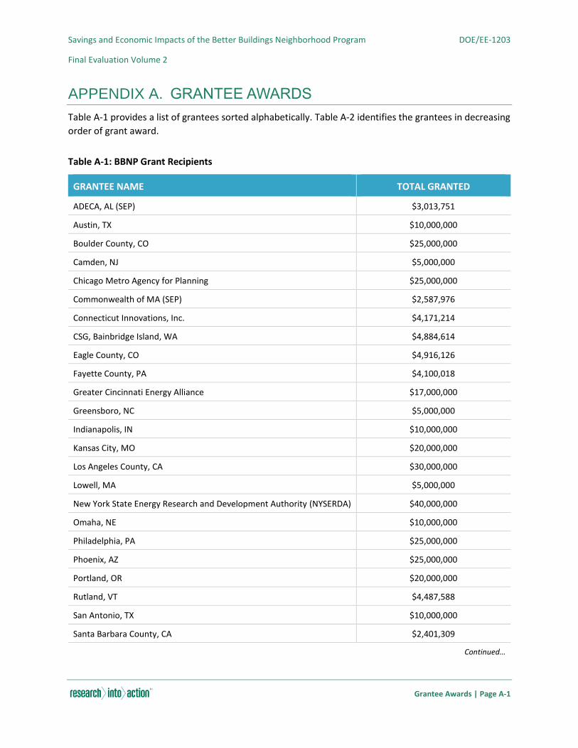
Savings and Economic Impacts of the Better Buildings Neighborhood Program DOE/EE-1203
Final Evaluation Volume 2
Grantee Awards | Page A-1
APPENDIX A. GRANTEE AWARDS
Table A-1 provides a list of grantees sorted alphabetically. Table A-2 identifies the grantees in decreasing
order of grant award.
Table A-1: BBNP Grant Recipients
GRANTEE NAME TOTAL GRANTED
ADECA, AL (SEP) $3,013,751
Austin, TX $10,000,000
Boulder County, CO $25,000,000
Camden, NJ $5,000,000
Chicago Metro Agency for Planning $25,000,000
Commonwealth of MA (SEP) $2,587,976
Connecticut Innovations, Inc. $4,171,214
CSG, Bainbridge Island, WA $4,884,614
Eagle County, CO $4,916,126
Fayette County, PA $4,100,018
Greater Cincinnati Energy Alliance $17,000,000
Greensboro, NC $5,000,000
Indianapolis, IN $10,000,000
Kansas City, MO $20,000,000
Los Angeles County, CA $30,000,000
Lowell, MA $5,000,000
New York State Energy Research and Development Authority (NYSERDA) $40,000,000
Omaha, NE $10,000,000
Philadelphia, PA $25,000,000
Phoenix, AZ $25,000,000
Portland, OR $20,000,000
Rutland, VT $4,487,588
San Antonio, TX $10,000,000
Santa Barbara County, CA $2,401,309
Continued…
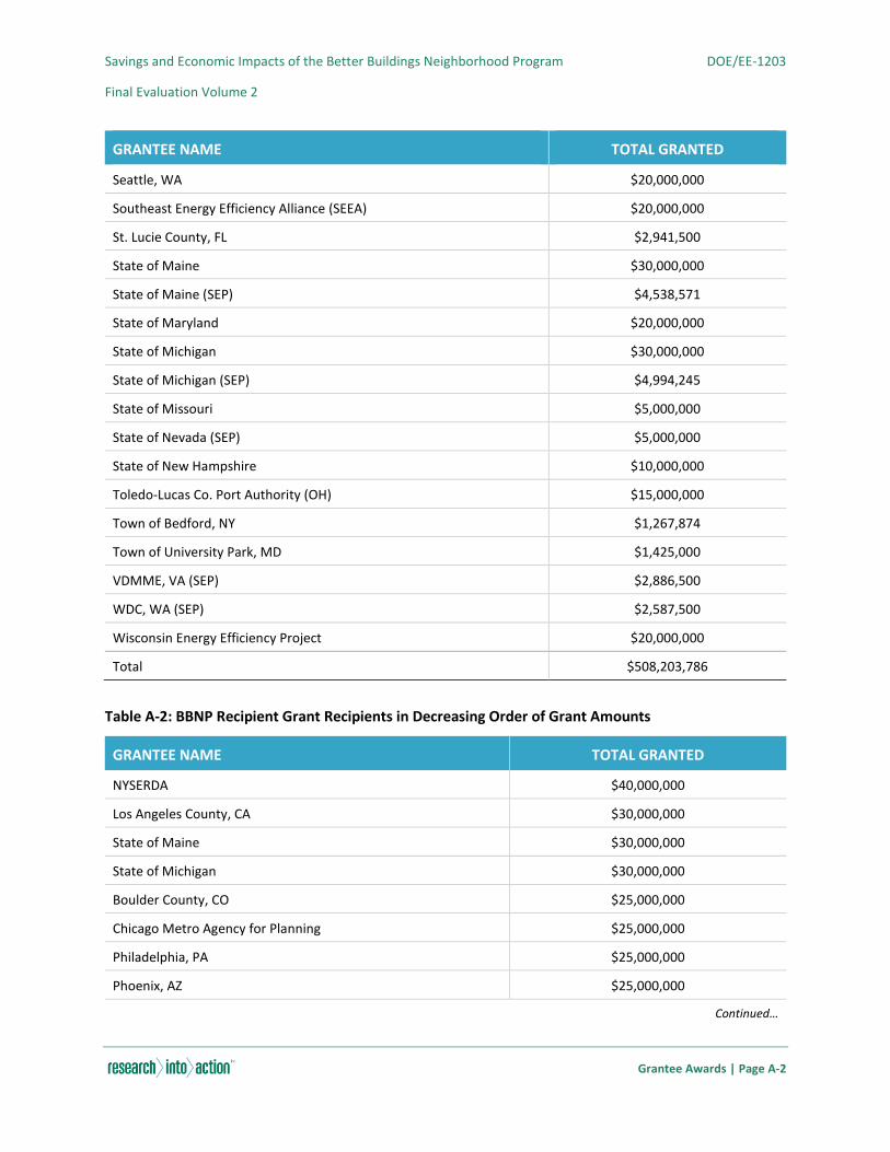
Savings and Economic Impacts of the Better Buildings Neighborhood Program DOE/EE-1203
Final Evaluation Volume 2
Grantee Awards | Page A-2
GRANTEE NAME TOTAL GRANTED
Seattle, WA $20,000,000
Southeast Energy Efficiency Alliance (SEEA) $20,000,000
St. Lucie County, FL $2,941,500
State of Maine $30,000,000
State of Maine (SEP) $4,538,571
State of Maryland $20,000,000
State of Michigan $30,000,000
State of Michigan (SEP) $4,994,245
State of Missouri $5,000,000
State of Nevada (SEP) $5,000,000
State of New Hampshire $10,000,000
Toledo-Lucas Co. Port Authority (OH) $15,000,000
Town of Bedford, NY $1,267,874
Town of University Park, MD $1,425,000
VDMME, VA (SEP) $2,886,500
WDC, WA (SEP) $2,587,500
Wisconsin Energy Efficiency Project $20,000,000
Total $508,203,786
Table A-2: BBNP Recipient Grant Recipients in Decreasing Order of Grant Amounts
GRANTEE NAME TOTAL GRANTED
NYSERDA $40,000,000
Los Angeles County, CA $30,000,000
State of Maine $30,000,000
State of Michigan $30,000,000
Boulder County, CO $25,000,000
Chicago Metro Agency for Planning $25,000,000
Philadelphia, PA $25,000,000
Phoenix, AZ $25,000,000
Continued…
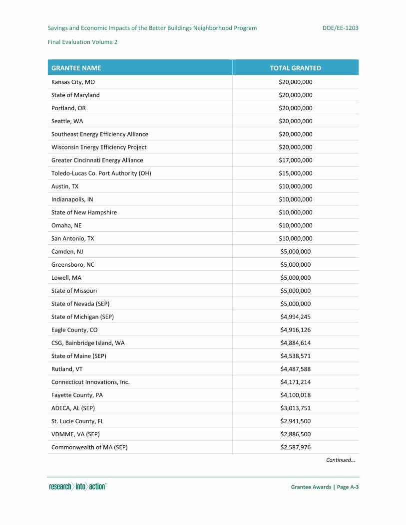
Savings and Economic Impacts of the Better Buildings Neighborhood Program DOE/EE-1203
Final Evaluation Volume 2
Grantee Awards | Page A-3
GRANTEE NAME TOTAL GRANTED
Kansas City, MO $20,000,000
State of Maryland $20,000,000
Portland, OR $20,000,000
Seattle, WA $20,000,000
Southeast Energy Efficiency Alliance $20,000,000
Wisconsin Energy Efficiency Project $20,000,000
Greater Cincinnati Energy Alliance $17,000,000
Toledo-Lucas Co. Port Authority (OH) $15,000,000
Austin, TX $10,000,000
Indianapolis, IN $10,000,000
State of New Hampshire $10,000,000
Omaha, NE $10,000,000
San Antonio, TX $10,000,000
Camden, NJ $5,000,000
Greensboro, NC $5,000,000
Lowell, MA $5,000,000
State of Missouri $5,000,000
State of Nevada (SEP) $5,000,000
State of Michigan (SEP) $4,994,245
Eagle County, CO $4,916,126
CSG, Bainbridge Island, WA $4,884,614
State of Maine (SEP) $4,538,571
Rutland, VT $4,487,588
Connecticut Innovations, Inc. $4,171,214
Fayette County, PA $4,100,018
ADECA, AL (SEP) $3,013,751
St. Lucie County, FL $2,941,500
VDMME, VA (SEP) $2,886,500
Commonwealth of MA (SEP) $2,587,976
Continued…

Savings and Economic Impacts of the Better Buildings Neighborhood Program DOE/EE-1203
Final Evaluation Volume 2
Grantee Awards | Page A-4
GRANTEE NAME TOTAL GRANTED
WDC, WA (SEP) $2,587,500
Santa Barbara County, CA $2,401,309
Town of University Park, MD $1,425,000
Town of Bedford, NY $1,267,874
Total $508,203,786
Savings and Economic Impacts of the Better Buildings Neighborhood Program DOE/EE-1203
Final Evaluation Volume 2
Impact Evaluation Methodology Supplement | Page B-1
APPENDIX B. IMPACT EVALUATION METHODOLOGY
SUPPLEMENT
B.1. OVERVIEW
Impact evaluations of efficiency programs seek to quantify the gross and net energy savings that have
been realized by projects enrolled in a program.
The team utilized a sector based analysis (that is, residential, multifamily and commercial) that reviewed
savings associated with individual projects, not the individual measures making up each project.
Because it was not cost-effective to complete analysis and onsite inspections on a census of the
programs and the program projects, savings were only verified for a representative sample of projects.
We also conducted a billing regression analysis to estimate realized energy savings at the project level.
The scale of this billing regression analysis depended on the availability of sufficient pre- and post-
installation utility billing data for a large enough sample of end-use customers to support a regression
model. Finally, we employed multiple approaches to develop an estimate of net savings, the proportion
of reported savings that were actually caused by the program. This work allows U.S. Department of
Energy (DOE) to report its best estimate for the energy savings actually achieved by the Better Buildings
Neighborhood Program (BBNP) program, based on Measurement and Verification (M&V), billing
regression, and net savings analyses that use detailed data collected about actual retrofit activities,
energy use, and decision-making based on representative samples of program projects and market
participants.
Finally, the final impact evaluation estimated the economic impacts of BBNP. These impacts included
jobs, as well as estimates of economic output, income (personal and business), and tax revenue that
resulted from the program spending relative to a base case scenario where BBNP did not exist.
B.1.1. COMPONENTS OF THE RESEARCH The impact evaluation for BBNP encompassed the following activities, each of which is outlined in
greater detail throughout this section:
Develop Sample Approach
Design the M&V Sample
Conduct M&V
Conduct Billing regression analysis Regression
Review of Independent Evaluations
Net-to-Gross (NTG) Analysis
Extrapolation of Results to Overall BBNP Level
Calculate Additional Metrics

Savings and Economic Impacts of the Better Buildings Neighborhood Program DOE/EE-1203
Final Evaluation Volume 2
Impact Evaluation Methodology Supplement | Page B-2
Economic Impacts Analysis
The impact evaluation team relied on their collective experiences conducting evaluations, along with
information gathered from externally published protocols and guidelines for reference and guidance
throughout the evaluation project. Secondary sources included:
The 2004 California Evaluation Framework (TecMarket Works, 2004).
Model Energy-Efficiency Program Impact Evaluation Guide (Schiller Consulting, 2007).
Uniform Methods Project38
Impact Evaluation Framework for Technology Deployment Programs (Reed, Jordan, and Vine,
2007).
Conference papers available through the International Energy Program Evaluation Conference
(IEPEC)39
“An Evaluation Approach for Assessing Program Performance from the State Energy Program”40
International Performance Measurement and Verification Protocol (IPMVP®)41
B.1.2. TIMING OF EVALUATION ACTIVITIES The preliminary evaluation commenced February 2012, and the results of the preliminary evaluation
were presented in July of 2013. The final evaluation activities commenced in summer 2013 with the
development of the draft Final Evaluation Plan. The Plan was submitted in September for review and
comment by DOE and a peer review group consisting of experts in the energy efficiency evaluation field.
Based on feedback from DOE, we finalized the Evaluation Plan in November 2013 (Research Into Action,
Evergreen Economics, Nexant, Inc., and NMR Group, Inc., 2013). Following DOE approval of the Plan, the
impact evaluation activities commenced with the sampling process, data collection, billing regression
analysis, verification activities, and the economic analysis. Table B-1 provides a summary of the major
activities and deliverables associated with both the preliminary and final impact evaluation.
Table B-1: Summary of Major Final Impact Evaluation Project Deliverables
ACTIVITIES AND DELIVERABLES DATE
Preliminary Evaluation Kick-Off February 2012
Grantee Interviews July – August 2012
Preliminary Evaluation Plan January 2013
38 For a full copy of the Uniform Methods Project protocols see: http://www1.eere.energy.gov/deployment/ump.html
39 See: www.iepec.org.
40 Written in collaboration by TecMarket Works, NYSERDA, Megdal & Associates, Edward Vine, and Marty Kushler.
41 2010. International Performance Measurement and Verification Protocol. Efficiency Valuation Organization (EVO®).

Savings and Economic Impacts of the Better Buildings Neighborhood Program DOE/EE-1203
Final Evaluation Volume 2
Impact Evaluation Methodology Supplement | Page B-3
ACTIVITIES AND DELIVERABLES DATE
Preliminary Evaluation Findings and Report July 2013
Final Evaluation Plan November 2013
Final Evaluation Report June 2015
We used two major approaches for determining gross savings: utility bill regression analysis and M&V
on a sample of grantee projects. Table B-2 outlines the specific tasks and timelines associated with these
approaches.
Table B-2: Schedule of Major Evaluation Activities
IMPACT EVALUATION ACTIVITIES DATE
Preliminary Evaluation
Database and Project File Review January - March 2013
Billing Data Requests February 2013
Grantee Data Requests February - March 2013
Participant Verification Phone Surveys March - April 2013
Onsite Verification Surveys April 2013
Billing regression analysis March - May 2013
Economic Analysis March - May 2013
M&V Analysis May 2013
Report Writing May - June 2013
Final Evaluation
Database and Project File Review December 2013 – January 2014
Billing Data Requests October 2013 – May 2014
Onsite Verification Surveys February – April 2014
Grantee Data Requests February – July 2014
Billing regression analysis October 2014
Economic Analysis October 2014
M&V Analysis August – October 2014
Report Writing November 2014 – June 2015
Savings and Economic Impacts of the Better Buildings Neighborhood Program DOE/EE-1203
Final Evaluation Volume 2
Impact Evaluation Methodology Supplement | Page B-4
B.1.3. RELATIONSHIP TO PRELIMINARY EVALUATION METHODOLOGY We conducted two impact evaluations as part of this Project; the preliminary evaluation that measured
impacts through the second quarter of 2012, and the final evaluation that continued the impact
evaluation activities through Q3 2013 The goal of the preliminary evaluation was to not only provide
impact results mid-way through the BBNP program cycle, support the process evaluation activities, and
to coordinate with other evaluation activities, but also to inform us about methods that worked and
processes that might be implemented by the grantees to allow for an effective final impact evaluation.
The final impact evaluation focused on verifying the sample of grantee reported activities after Q2 2012
as well as leveraging results from the preliminary evaluation in order to quantify impact metrics for the
entire grant cycle of the BBNP.
B.2. SAMPLING METHODS
The evaluation of BBNP is unique due to the program’s significant scope, size, and reporting
methodology. As discussed, grantees collected and reported a wide range of information, and the team
worked to design a flexible methodology that handled the variety of information that was available. The
sampling methods employed for the impact evaluation took into account the two distinct activities
utilized to determine gross verified savings:
M&V of a sample of grantees and projects
Billing regression analysis on projects from grantees with sufficient utility bill data
Ultimately, the results from both activities were combined and extrapolated to the population in order
to determine the overall estimated energy savings for BBNP. Details regarding the methodology for
combining and extrapolating the results are provided later in this section.
B.2.1. OVERVIEW OF M&V AND REGRESSION SAMPLING APPROACHES Unique sample frames were selected for each evaluation activity. The billing regression sample was
based on the availability of sufficient grantee billing data required to conduct the billing regression
analysis. Table 3-1 outlines the sample frame for the preliminary and final evaluation by evaluation
activity.
B.2.2. OVERLAP OF M&V AND REGRESSION SAMPLES For the final evaluation, the team overlapped sampled grantees between the M&V and billing regression
analysis sample frames. The intention of this overlap was to understand the differences on estimated
savings when using M&V versus billing regression, normalize those differences, and merge the M&V and
billing analyses to calculate an overall realization rate for the BBNP. Further discussion on the
adjustments we made in order to merge the M&V and billing analyses is provided in Appendix B, Section
B.7.3.
B.2.3. M&V SAMPLE The sampling provided a high level of project verification coupled with an efficient use of onsite
activities to achieve an industry-standard level of measurement rigor. Verification of energy savings and
influence/ spillover surveys conducted throughout the preliminary and final M&V activities included

Savings and Economic Impacts of the Better Buildings Neighborhood Program DOE/EE-1203
Final Evaluation Volume 2
Impact Evaluation Methodology Supplement | Page B-5
participant telephone surveys (conducted only for the preliminary evaluation), detailed desk review and
analysis, and onsite inspections (conducted on a smaller subset of the sample population).
Sample Parameters
Three key parameters were established for an effective sample design of the M&V population:
Confidence
Precision
Coefficient of Variance (Cv)
Confidence and Precision The industry standard confidence and precision levels for energy efficiency program evaluations is 90%
confidence, with 10% precision. The sampling strategy was designed to meet 90/10 confidence and
precision at the overall BBNP level.
Coefficient of Variance
The greater the deviation of the observed value from the reported value, the greater is the variance in
the sample pool. A greater variance in the sample pool indicates poor correlation between ex ante and
ex-post savings and the potential need to sample more data points in order to reduce the error ratios in
the sample pools. If a greater variance is expected in the reported impacts, the Cv is set at a higher value
at the beginning of the sampling process, resulting in a larger sample pool.42
During planning for the preliminary evaluation, we determined that there was a strong likelihood for a
larger deviation in reported savings. In order to address this issue, the Cv used for setting the sample
size was set at 1.2 for the entire BBNP during the preliminary evaluation. Utility evaluations generally
use a Cv of .5 for the majority of evaluations, as their programs are generally focused on specific
measures and have established standardized reporting and measurement procedures. By establishing a
higher Cv, we acknowledged the challenges listed below and selected a larger sample size to account for
the perceived higher variability in the reported results.
Grantee’s challenges with reporting project savings
Errors in the reporting documents
DOE’s challenges in capturing data in different formats
Changes in reporting requirements since the programs began
Lack of grantee experience managing energy efficiency programs
42 The Cv is an estimate of the variability of the population in relation to the mean. Populations with assumed higher Cv indicates
a larger sample size will be necessary in order to achieve the desired confidence and precision due to variability in the reported
findings.
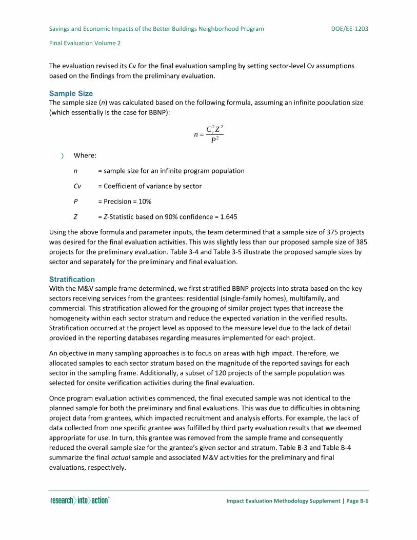
Savings and Economic Impacts of the Better Buildings Neighborhood Program DOE/EE-1203
Final Evaluation Volume 2
Impact Evaluation Methodology Supplement | Page B-6
The evaluation revised its Cv for the final evaluation sampling by setting sector-level Cv assumptions
based on the findings from the preliminary evaluation.
Sample Size
The sample size (n) was calculated based on the following formula, assuming an infinite population size
(which essentially is the case for BBNP):
Where:
n = sample size for an infinite program population
Cv = Coefficient of variance by sector
P = Precision = 10%
Z = Z-Statistic based on 90% confidence = 1.645
Using the above formula and parameter inputs, the team determined that a sample size of 375 projects
was desired for the final evaluation activities. This was slightly less than our proposed sample size of 385
projects for the preliminary evaluation. Table 3-4 and Table 3-5 illustrate the proposed sample sizes by
sector and separately for the preliminary and final evaluation.
Stratification
With the M&V sample frame determined, we first stratified BBNP projects into strata based on the key
sectors receiving services from the grantees: residential (single-family homes), multifamily, and
commercial. This stratification allowed for the grouping of similar project types that increase the
homogeneity within each sector stratum and reduce the expected variation in the verified results.
Stratification occurred at the project level as opposed to the measure level due to the lack of detail
provided in the reporting databases regarding measures implemented for each project.
An objective in many sampling approaches is to focus on areas with high impact. Therefore, we
allocated samples to each sector stratum based on the magnitude of the reported savings for each
sector in the sampling frame. Additionally, a subset of 120 projects of the sample population was
selected for onsite verification activities during the final evaluation.
Once program evaluation activities commenced, the final executed sample was not identical to the
planned sample for both the preliminary and final evaluations. This was due to difficulties in obtaining
project data from grantees, which impacted recruitment and analysis efforts. For example, the lack of
data collected from one specific grantee was fulfilled by third party evaluation results that we deemed
appropriate for use. In turn, this grantee was removed from the sample frame and consequently
reduced the overall sample size for the grantee’s given sector and stratum. Table B-3 and Table B-4
summarize the final actual sample and associated M&V activities for the preliminary and final
evaluations, respectively.
2
22
P
ZCn v
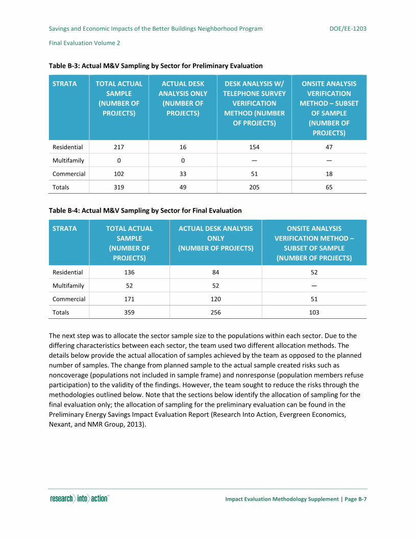
Savings and Economic Impacts of the Better Buildings Neighborhood Program DOE/EE-1203
Final Evaluation Volume 2
Impact Evaluation Methodology Supplement | Page B-7
Table B-3: Actual M&V Sampling by Sector for Preliminary Evaluation
STRATA TOTAL ACTUAL
SAMPLE
(NUMBER OF
PROJECTS)
ACTUAL DESK
ANALYSIS ONLY
(NUMBER OF
PROJECTS)
DESK ANALYSIS W/
TELEPHONE SURVEY
VERIFICATION
METHOD (NUMBER
OF PROJECTS)
ONSITE ANALYSIS
VERIFICATION
METHOD – SUBSET
OF SAMPLE
(NUMBER OF
PROJECTS)
Residential 217 16 154 47
Multifamily 0 0 — —
Commercial 102 33 51 18
Totals 319 49 205 65
Table B-4: Actual M&V Sampling by Sector for Final Evaluation
STRATA TOTAL ACTUAL
SAMPLE
(NUMBER OF
PROJECTS)
ACTUAL DESK ANALYSIS
ONLY
(NUMBER OF PROJECTS)
ONSITE ANALYSIS
VERIFICATION METHOD –
SUBSET OF SAMPLE
(NUMBER OF PROJECTS)
Residential 136 84 52
Multifamily 52 52 —
Commercial 171 120 51
Totals 359 256 103
The next step was to allocate the sector sample size to the populations within each sector. Due to the
differing characteristics between each sector, the team used two different allocation methods. The
details below provide the actual allocation of samples achieved by the team as opposed to the planned
number of samples. The change from planned sample to the actual sample created risks such as
noncoverage (populations not included in sample frame) and nonresponse (population members refuse
participation) to the validity of the findings. However, the team sought to reduce the risks through the
methodologies outlined below. Note that the sections below identify the allocation of sampling for the
final evaluation only; the allocation of sampling for the preliminary evaluation can be found in the
Preliminary Energy Savings Impact Evaluation Report (Research Into Action, Evergreen Economics,
Nexant, and NMR Group, 2013).
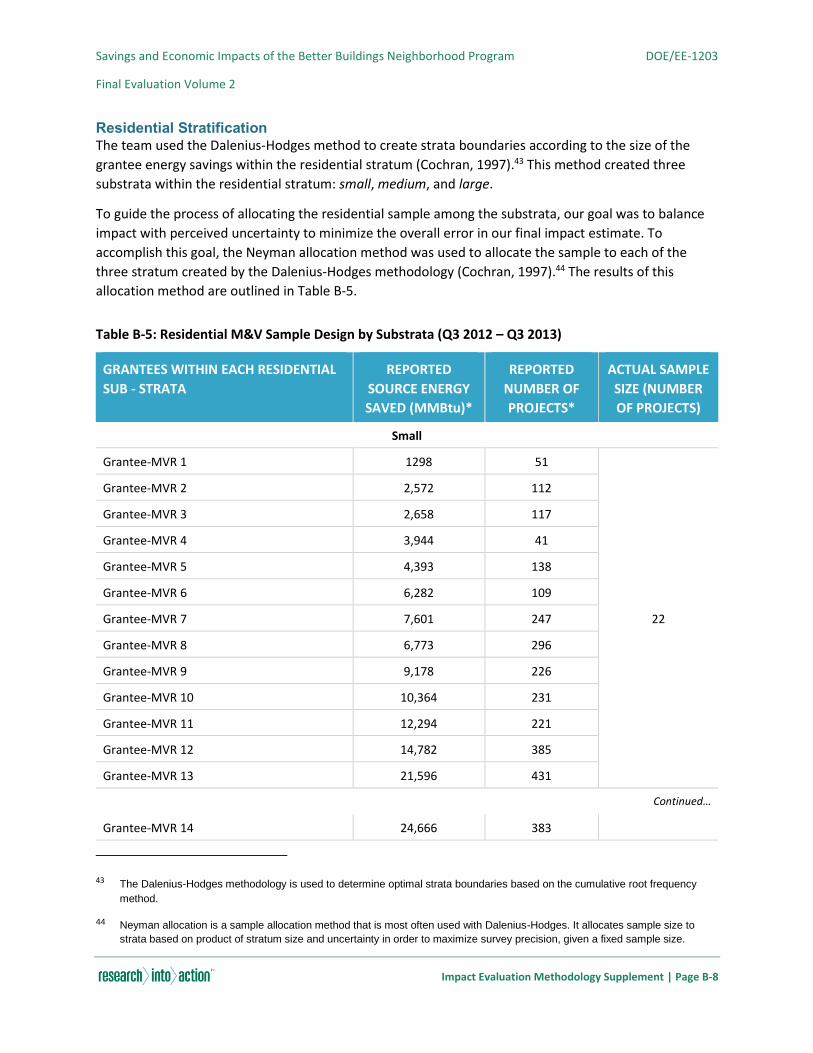
Savings and Economic Impacts of the Better Buildings Neighborhood Program DOE/EE-1203
Final Evaluation Volume 2
Impact Evaluation Methodology Supplement | Page B-8
Residential Stratification The team used the Dalenius-Hodges method to create strata boundaries according to the size of the
grantee energy savings within the residential stratum (Cochran, 1997).43 This method created three
substrata within the residential stratum: small, medium, and large.
To guide the process of allocating the residential sample among the substrata, our goal was to balance
impact with perceived uncertainty to minimize the overall error in our final impact estimate. To
accomplish this goal, the Neyman allocation method was used to allocate the sample to each of the
three stratum created by the Dalenius-Hodges methodology (Cochran, 1997).44 The results of this
allocation method are outlined in Table B-5.
Table B-5: Residential M&V Sample Design by Substrata (Q3 2012 – Q3 2013)
GRANTEES WITHIN EACH RESIDENTIAL
SUB - STRATA
REPORTED
SOURCE ENERGY
SAVED (MMBtu)*
REPORTED
NUMBER OF
PROJECTS*
ACTUAL SAMPLE
SIZE (NUMBER
OF PROJECTS)
Small
Grantee-MVR 1 1298 51
22
Grantee-MVR 2 2,572 112
Grantee-MVR 3 2,658 117
Grantee-MVR 4 3,944 41
Grantee-MVR 5 4,393 138
Grantee-MVR 6 6,282 109
Grantee-MVR 7 7,601 247
Grantee-MVR 8 6,773 296
Grantee-MVR 9 9,178 226
Grantee-MVR 10 10,364 231
Grantee-MVR 11 12,294 221
Grantee-MVR 12 14,782 385
Grantee-MVR 13 21,596 431
Continued…
Grantee-MVR 14 24,666 383
43 The Dalenius-Hodges methodology is used to determine optimal strata boundaries based on the cumulative root frequency
method.
44 Neyman allocation is a sample allocation method that is most often used with Dalenius-Hodges. It allocates sample size to
strata based on product of stratum size and uncertainty in order to maximize survey precision, given a fixed sample size.
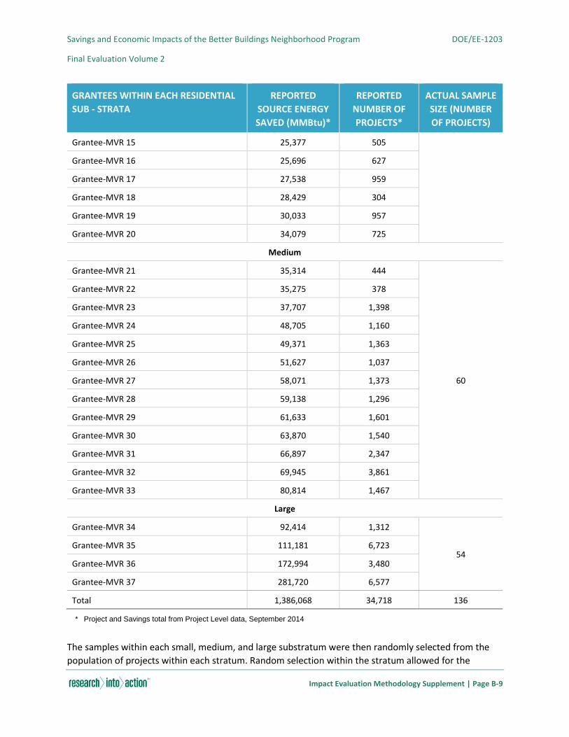
Savings and Economic Impacts of the Better Buildings Neighborhood Program DOE/EE-1203
Final Evaluation Volume 2
Impact Evaluation Methodology Supplement | Page B-9
GRANTEES WITHIN EACH RESIDENTIAL
SUB - STRATA
REPORTED
SOURCE ENERGY
SAVED (MMBtu)*
REPORTED
NUMBER OF
PROJECTS*
ACTUAL SAMPLE
SIZE (NUMBER
OF PROJECTS)
Grantee-MVR 15 25,377 505
Grantee-MVR 16 25,696 627
Grantee-MVR 17 27,538 959
Grantee-MVR 18 28,429 304
Grantee-MVR 19 30,033 957
Grantee-MVR 20 34,079 725
Medium
Grantee-MVR 21 35,314 444
60
Grantee-MVR 22 35,275 378
Grantee-MVR 23 37,707 1,398
Grantee-MVR 24 48,705 1,160
Grantee-MVR 25 49,371 1,363
Grantee-MVR 26 51,627 1,037
Grantee-MVR 27 58,071 1,373
Grantee-MVR 28 59,138 1,296
Grantee-MVR 29 61,633 1,601
Grantee-MVR 30 63,870 1,540
Grantee-MVR 31 66,897 2,347
Grantee-MVR 32 69,945 3,861
Grantee-MVR 33 80,814 1,467
Large
Grantee-MVR 34 92,414 1,312
54 Grantee-MVR 35 111,181 6,723
Grantee-MVR 36 172,994 3,480
Grantee-MVR 37 281,720 6,577
Total 1,386,068 34,718 136
* Project and Savings total from Project Level data, September 2014
The samples within each small, medium, and large substratum were then randomly selected from the
population of projects within each stratum. Random selection within the stratum allowed for the
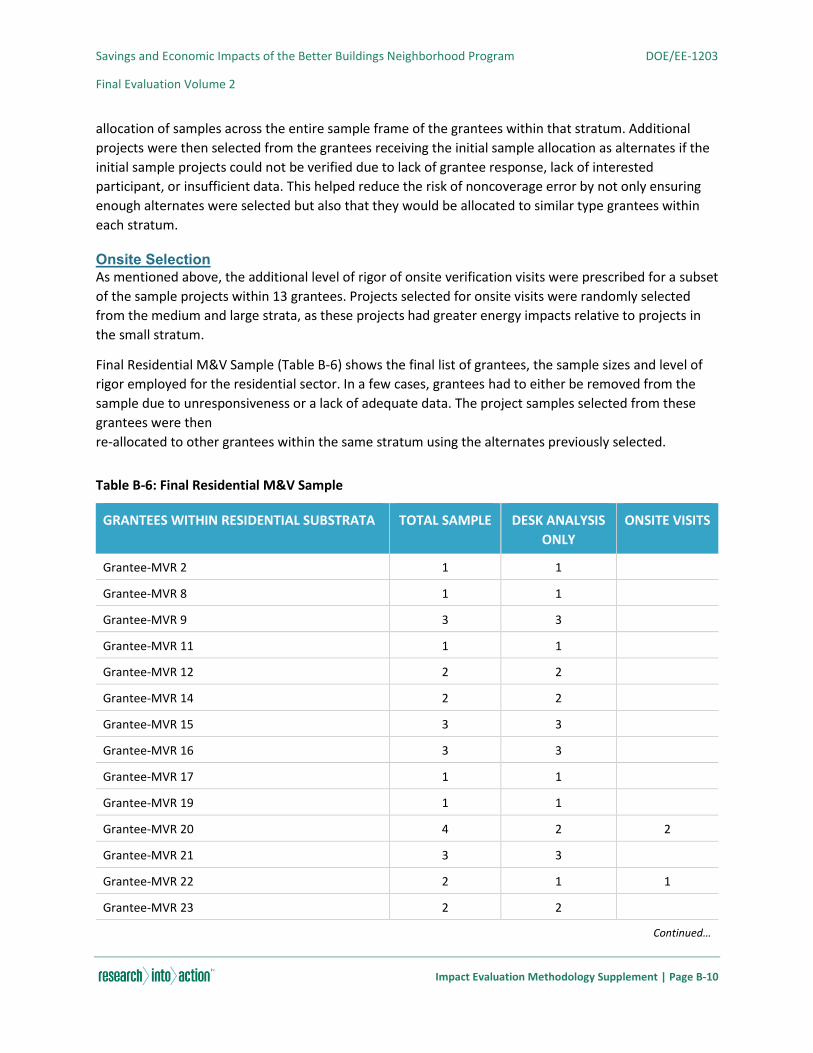
Savings and Economic Impacts of the Better Buildings Neighborhood Program DOE/EE-1203
Final Evaluation Volume 2
Impact Evaluation Methodology Supplement | Page B-10
allocation of samples across the entire sample frame of the grantees within that stratum. Additional
projects were then selected from the grantees receiving the initial sample allocation as alternates if the
initial sample projects could not be verified due to lack of grantee response, lack of interested
participant, or insufficient data. This helped reduce the risk of noncoverage error by not only ensuring
enough alternates were selected but also that they would be allocated to similar type grantees within
each stratum.
Onsite Selection
As mentioned above, the additional level of rigor of onsite verification visits were prescribed for a subset
of the sample projects within 13 grantees. Projects selected for onsite visits were randomly selected
from the medium and large strata, as these projects had greater energy impacts relative to projects in
the small stratum.
Final Residential M&V Sample (Table B-6) shows the final list of grantees, the sample sizes and level of
rigor employed for the residential sector. In a few cases, grantees had to either be removed from the
sample due to unresponsiveness or a lack of adequate data. The project samples selected from these
grantees were then
re-allocated to other grantees within the same stratum using the alternates previously selected.
Table B-6: Final Residential M&V Sample
GRANTEES WITHIN RESIDENTIAL SUBSTRATA TOTAL SAMPLE DESK ANALYSIS
ONLY
ONSITE VISITS
Grantee-MVR 2 1 1
Grantee-MVR 8 1 1
Grantee-MVR 9 3 3
Grantee-MVR 11 1 1
Grantee-MVR 12 2 2
Grantee-MVR 14 2 2
Grantee-MVR 15 3 3
Grantee-MVR 16 3 3
Grantee-MVR 17 1 1
Grantee-MVR 19 1 1
Grantee-MVR 20 4 2 2
Grantee-MVR 21 3 3
Grantee-MVR 22 2 1 1
Grantee-MVR 23 2 2
Continued…
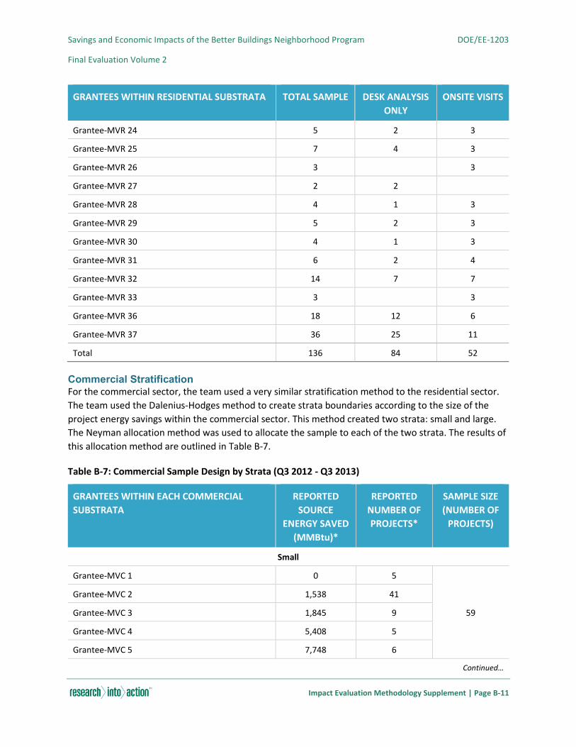
Savings and Economic Impacts of the Better Buildings Neighborhood Program DOE/EE-1203
Final Evaluation Volume 2
Impact Evaluation Methodology Supplement | Page B-11
GRANTEES WITHIN RESIDENTIAL SUBSTRATA TOTAL SAMPLE DESK ANALYSIS
ONLY
ONSITE VISITS
Grantee-MVR 24 5 2 3
Grantee-MVR 25 7 4 3
Grantee-MVR 26 3 3
Grantee-MVR 27 2 2
Grantee-MVR 28 4 1 3
Grantee-MVR 29 5 2 3
Grantee-MVR 30 4 1 3
Grantee-MVR 31 6 2 4
Grantee-MVR 32 14 7 7
Grantee-MVR 33 3 3
Grantee-MVR 36 18 12 6
Grantee-MVR 37 36 25 11
Total 136 84 52
Commercial Stratification For the commercial sector, the team used a very similar stratification method to the residential sector.
The team used the Dalenius-Hodges method to create strata boundaries according to the size of the
project energy savings within the commercial sector. This method created two strata: small and large.
The Neyman allocation method was used to allocate the sample to each of the two strata. The results of
this allocation method are outlined in Table B-7.
Table B-7: Commercial Sample Design by Strata (Q3 2012 - Q3 2013)
GRANTEES WITHIN EACH COMMERCIAL
SUBSTRATA
REPORTED
SOURCE
ENERGY SAVED
(MMBtu)*
REPORTED
NUMBER OF
PROJECTS*
SAMPLE SIZE
(NUMBER OF
PROJECTS)
Small
Grantee-MVC 1 0 5
59
Grantee-MVC 2 1,538 41
Grantee-MVC 3 1,845 9
Grantee-MVC 4 5,408 5
Grantee-MVC 5 7,748 6
Continued…
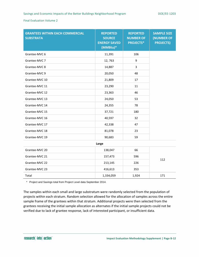
Savings and Economic Impacts of the Better Buildings Neighborhood Program DOE/EE-1203
Final Evaluation Volume 2
Impact Evaluation Methodology Supplement | Page B-12
GRANTEES WITHIN EACH COMMERCIAL
SUBSTRATA
REPORTED
SOURCE
ENERGY SAVED
(MMBtu)*
REPORTED
NUMBER OF
PROJECTS*
SAMPLE SIZE
(NUMBER OF
PROJECTS)
Grantee-MVC 6 11,391 106
Grantee-MVC 7 12, 763 9
Grantee-MVC 8 14,887 3
Grantee-MVC 9 20,050 48
Grantee-MVC 10 21,809 17
Grantee-MVC 11 23,290 11
Grantee-MVC 12 23,363 46
Grantee-MVC 13 24,050 53
Grantee-MVC 14 24,355 78
Grantee-MVC 15 37,721 180
Grantee-MVC 16 40,597 32
Grantee-MVC 17 42,338 47
Grantee-MVC 18 81,078 23
Grantee-MVC 19 90,683 59
Large
Grantee-MVC 20 138,047 66
112 Grantee-MVC 21 157,473 596
Grantee-MVC 22 213,145 226
Grantee-MVC 23 416,613 353
Total 1,334,059 1,924 171
* Project and Savings total from Project Level data September 2014.
The samples within each small and large substratum were randomly selected from the population of
projects within each stratum. Random selection allowed for the allocation of samples across the entire
sample frame of the grantees within that stratum. Additional projects were then selected from the
grantees receiving the initial sample allocation as alternates if the initial sample projects could not be
verified due to lack of grantee response, lack of interested participant, or insufficient data.
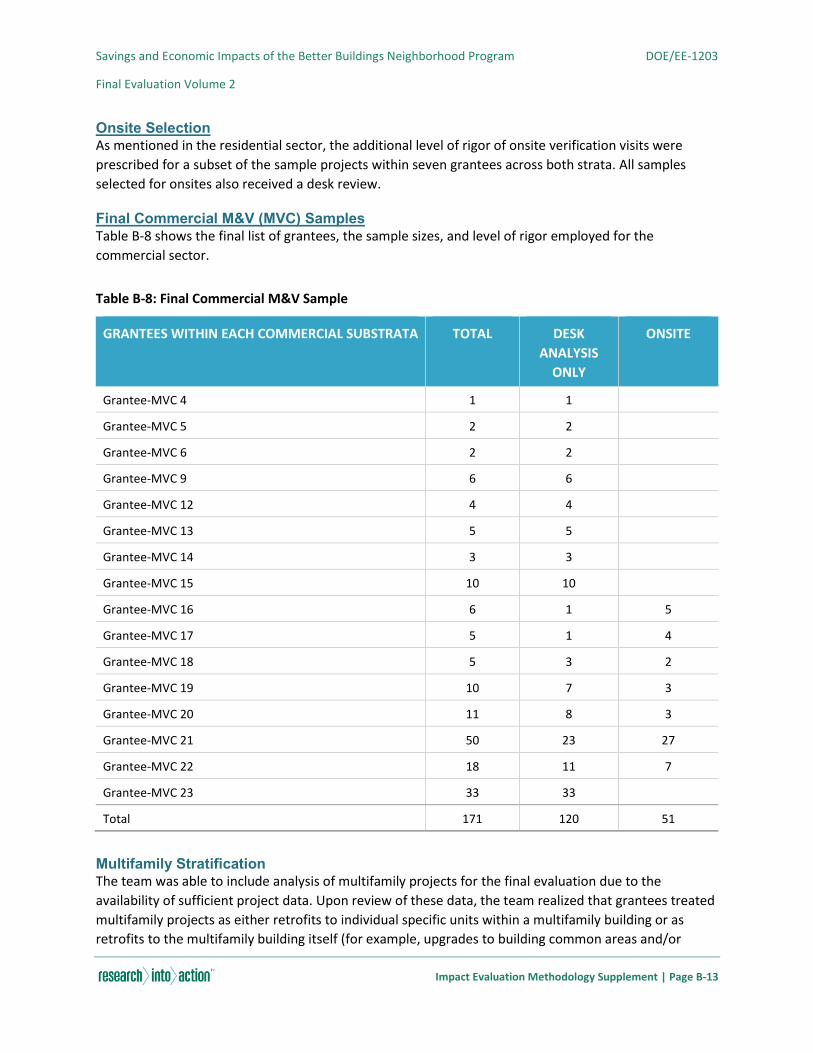
Savings and Economic Impacts of the Better Buildings Neighborhood Program DOE/EE-1203
Final Evaluation Volume 2
Impact Evaluation Methodology Supplement | Page B-13
Onsite Selection As mentioned in the residential sector, the additional level of rigor of onsite verification visits were
prescribed for a subset of the sample projects within seven grantees across both strata. All samples
selected for onsites also received a desk review.
Final Commercial M&V (MVC) Samples
Table B-8 shows the final list of grantees, the sample sizes, and level of rigor employed for the
commercial sector.
Table B-8: Final Commercial M&V Sample
GRANTEES WITHIN EACH COMMERCIAL SUBSTRATA TOTAL DESK
ANALYSIS
ONLY
ONSITE
Grantee-MVC 4 1 1
Grantee-MVC 5 2 2
Grantee-MVC 6 2 2
Grantee-MVC 9 6 6
Grantee-MVC 12 4 4
Grantee-MVC 13 5 5
Grantee-MVC 14 3 3
Grantee-MVC 15 10 10
Grantee-MVC 16 6 1 5
Grantee-MVC 17 5 1 4
Grantee-MVC 18 5 3 2
Grantee-MVC 19 10 7 3
Grantee-MVC 20 11 8 3
Grantee-MVC 21 50 23 27
Grantee-MVC 22 18 11 7
Grantee-MVC 23 33 33
Total 171 120 51
Multifamily Stratification The team was able to include analysis of multifamily projects for the final evaluation due to the
availability of sufficient project data. Upon review of these data, the team realized that grantees treated
multifamily projects as either retrofits to individual specific units within a multifamily building or as
retrofits to the multifamily building itself (for example, upgrades to building common areas and/or
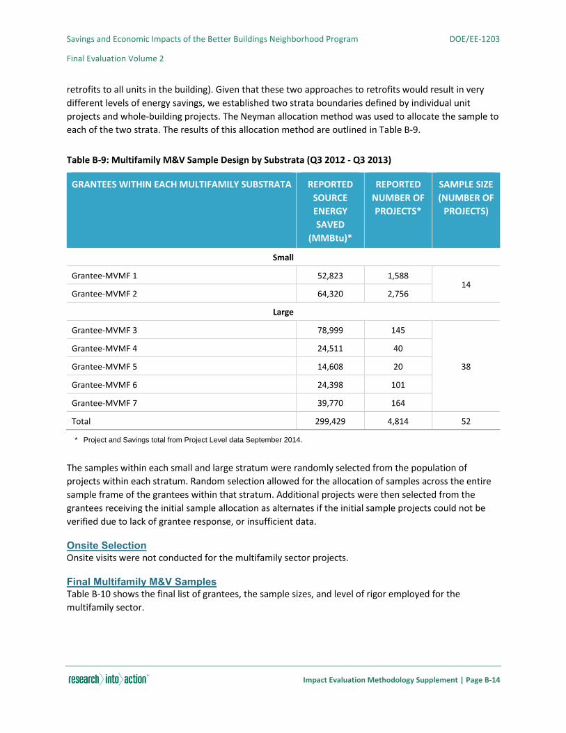
Savings and Economic Impacts of the Better Buildings Neighborhood Program DOE/EE-1203
Final Evaluation Volume 2
Impact Evaluation Methodology Supplement | Page B-14
retrofits to all units in the building). Given that these two approaches to retrofits would result in very
different levels of energy savings, we established two strata boundaries defined by individual unit
projects and whole-building projects. The Neyman allocation method was used to allocate the sample to
each of the two strata. The results of this allocation method are outlined in Table B-9.
Table B-9: Multifamily M&V Sample Design by Substrata (Q3 2012 - Q3 2013)
GRANTEES WITHIN EACH MULTIFAMILY SUBSTRATA REPORTED
SOURCE
ENERGY
SAVED
(MMBtu)*
REPORTED
NUMBER OF
PROJECTS*
SAMPLE SIZE
(NUMBER OF
PROJECTS)
Small
Grantee-MVMF 1 52,823 1,588 14
Grantee-MVMF 2 64,320 2,756
Large
Grantee-MVMF 3 78,999 145
38
Grantee-MVMF 4 24,511 40
Grantee-MVMF 5 14,608 20
Grantee-MVMF 6 24,398 101
Grantee-MVMF 7 39,770 164
Total 299,429 4,814 52
* Project and Savings total from Project Level data September 2014.
The samples within each small and large stratum were randomly selected from the population of
projects within each stratum. Random selection allowed for the allocation of samples across the entire
sample frame of the grantees within that stratum. Additional projects were then selected from the
grantees receiving the initial sample allocation as alternates if the initial sample projects could not be
verified due to lack of grantee response, or insufficient data.
Onsite Selection
Onsite visits were not conducted for the multifamily sector projects.
Final Multifamily M&V Samples
Table B-10 shows the final list of grantees, the sample sizes, and level of rigor employed for the
multifamily sector.

Savings and Economic Impacts of the Better Buildings Neighborhood Program DOE/EE-1203
Final Evaluation Volume 2
Impact Evaluation Methodology Supplement | Page B-15
Table B-10: Final Multifamily M&V (MVMF) Sample
GRANTEES WITHIN EACH MULTIFAMILY SUBSTRATA TOTAL DESK ANALYSIS
Small
Grantee-MVMF 1 5 5
Grantee-MVMF 2 9 9
Large
Grantee-MVMF 3 13 13
Grantee-MVMF 4 3 3
Grantee-MVMF 5 4 4
Grantee-MVMF 6 2 2
Grantee-MVMF 7 16 16
Total 52 52
B.3. MEASUREMENT AND VERIFICATION METHODS
The M&V activities conducted for the final impact evaluation included engineering review and
verification activities to determine the energy savings for a sample of projects. To determine the overall
estimated BBNP energy savings, the team used an ex-post analysis (actual savings based on post-retrofit
conditions) in order to estimate the energy savings for each project selected in the sample. Gross
verified energy savings were determined through information gathered from a combination of file
reviews and onsite inspections. Gross verified savings were compared to reported savings to determine
a realization rate for each sector.
Steps included in the verification approach, each of which is described in more detail in the following
sections, were:
Obtain Grantee Project Records
Design Onsite Survey and Data Collection Forms
Conduct Onsite Verifications
Conduct Project File Reviews
Establish Baseline Scenarios
Verify Gross Energy Savings.
B.3.1. OBTAINING GRANTEE PROJECT RECORDS The initial step of the evaluation activities involved obtaining DOE program records detailing the
reported savings and number of projects for each of the grantees. This involved the following key
sources of information:

Savings and Economic Impacts of the Better Buildings Neighborhood Program DOE/EE-1203
Final Evaluation Volume 2
Impact Evaluation Methodology Supplement | Page B-16
Project Level Database
Program Level Database from Quarterly Summary Reports
Measure Implementation Database
Grantee Quarterly Reports
We encountered challenges in determining the quality and accuracy of the data. Due to these
challenges, the team often used a triangulation approach to determine sources of inconsistency, areas
of concern, and overall quality of the data. We worked with representatives from DOE and National
Renewable Energy Laboratory (NREL) to correct errors, understand underlying issues, and interact with
the grantees to correct issues.
We selected the Project Level Database for use in determining the M&V sample and conducting the
impact analysis for energy savings for two main reasons:
1. The project data could be sorted into sectors to allow the team to determine savings and project
totals for each sector. The Program Level data did not have this option.
2. Interviews with some grantees indicated that the project level data was “more correct”
compared to the Program Level data.
Finally, the economic analysis utilized the Program Level Database, as this included specific metrics used
in the analysis, such as program expenditures, leveraged costs, and project costs. This information was
needed to conduct the economic analysis. The use of two different data sources for the analysis work in
this report created some discrepancies in the reporting of the results. These are noted where applicable.
B.3.2. DESIGNING THE DATA COLLECTION INSTRUMENTS Information gathered during the DOE data collection efforts informed the development of the surveys
and data collection forms used for onsite verification activities. Due to governmental policy regarding
population surveys, the team needed to undertake a number of steps to obtain approval to conduct
onsite verifications.
First, each surveyor needed to complete training from the Lawrence Berkeley National Laboratory
(LBNL) Environmental Health, Safety, and Security Division on Human Subjects Research. This training
ensured that staff understood the policies and procedures related to the surveying of populations.
Next, the team designed the onsite survey for both the residential and commercial sectors, as well as an
introduction letter to be sent to all potential participants in the sample. The surveys and introduction
letter were then sent to the LBNL Human Subjects Committee for approval.45 The surveys and approved
letter are included in Appendix J and Appendix K, respectively.
45 Federal regulations require that research involving human subjects or human derived data or tissues be reviewed by an
Institutional Review Board (IRB). At Lawrence Berkeley National Laboratory, the IRB is the Human Subjects Committee (HSC).
See: http://www.lbl.gov/ehs/health_services/harc/hsc.shtml

Savings and Economic Impacts of the Better Buildings Neighborhood Program DOE/EE-1203
Final Evaluation Volume 2
Impact Evaluation Methodology Supplement | Page B-17
Paper data collection forms were developed and used in the field during the onsite activities during the
final evaluation. All information gathered during the onsite inspections were entered into an internal
Microsoft Access tracking database that was designed to track results for all impact evaluation activities.
B.3.3. CONDUCTING ONSITE VERIFICATIONS Onsite inspections were conducted on a subset of sample projects in order to verify the accuracy of
information reported through project documentation files, to gather additional project details, and to
allow the team to note any discrepancies in reported versus actual project documentation. Typically,
onsite inspection activities included:
Collecting baseline (as available) and retrofit equipment information
Obtaining the operating parameters as applicable
Conducting a visual inspection
Gathering equipment nameplate information
Conducting brief onsite surveys with relevant parties to understand the facility or home
operation, equipment operating specifics, and other input parameters needed to calculate
energy savings. Additionally, a battery of net-to-gross questions was administered through the
onsite survey.
B.3.4. CONDUCTING PROJECT FILE REVIEWS Upon receipt of any documentation and project files for the sampled projects, we performed a file
review. The project-specific documents requested for the sampled projects included customer
applications, savings declarations performed by third party contractors (where applicable), pre- and
post-project audits, customer invoices, and other information as available and appropriate.
We then conducted a file review to answer the following questions:
Were the data files of sample projects complete and adequate to calculate and report savings?
Were the measures installed as described in the program tracking and reporting system?
Were input assumptions available, such as building size, building type, operating hours, etc.?
Were the savings accurately reported to DOE?
Finally, depending on the selected project, additional supporting information was requested from the
grantee, third party consultants, and implementation contractors when needed.
B.3.5. ESTABLISHING THE BASELINE SCENARIOS To provide an accurate and defensible evaluation of baseline characteristics, a triangulation approach
was utilized. We gathered and reviewed data from a variety of sources and reconciled the results to

Savings and Economic Impacts of the Better Buildings Neighborhood Program DOE/EE-1203
Final Evaluation Volume 2
Impact Evaluation Methodology Supplement | Page B-18
ensure that an accurate representation of the baseline characteristics was obtained. The following
sources were utilized depending on the information available from each grantee:
Application or Project Documents. Some grantees, through the use of applications for audit
reports, gathered pre-installation project information. When available and applicable, the team
used actual pre-installation information to calculate the ex-post energy savings.
Onsite Surveys. For a subset of the sample population, the team conducted onsite verification
of installed measures. During the onsite activities, questions were asked and observations were
made regarding baseline equipment condition, operating hours and parameters.
Local Codes and Standards Requirements. When information was not available via project
documentation, phone interviews, or onsite surveys, or when the installed measure was found
to be a replacement on burnout scenario, we used local energy and building code requirements
as the basis for determining the baseline condition.
Table B-11 outlines the baselines used for this analysis for the most common measures analyzed in the
sample.
Table B-11: Baseline Measure Data Used for Analysis
MEASURE BASELINE
Furnace 80 AFUE
Boiler 80 AFUE
Air Conditioner 13 SEER
Air Source Heat Pump 7.7 HSPF
Water Heater – Gas 0.575 EF
Water Heater – Electric 0.92 EF
Insulation – All locations Pre-existing conditions or R-5 if unknown
Compact Fluorescent Lamp (CFL) Direct
Install
Pre-existing lighting or 60W Incandescent if unknown
T8 Fluorescent Lamp Pre-existing lighting or T12 Fluorescent Lamp, 34W, 1.15 BF if
unknown
Air Sealing Pre-existing condition or 3600 CFM50 if unknown
Duct Sealing Pre-existing condition or 60% distribution efficiency if unknown
B.3.6. VERIFYING GROSS IMPACTS In order to calculate gross verified savings for each sampled project, the team created grantee-specific
analysis tools that used the information gathered during the file review and onsite inspections. The
team was challenged to create a consistent analysis methodology while working with grantees located
across the country in varied climate zones that offered a wide range of measures and may have been
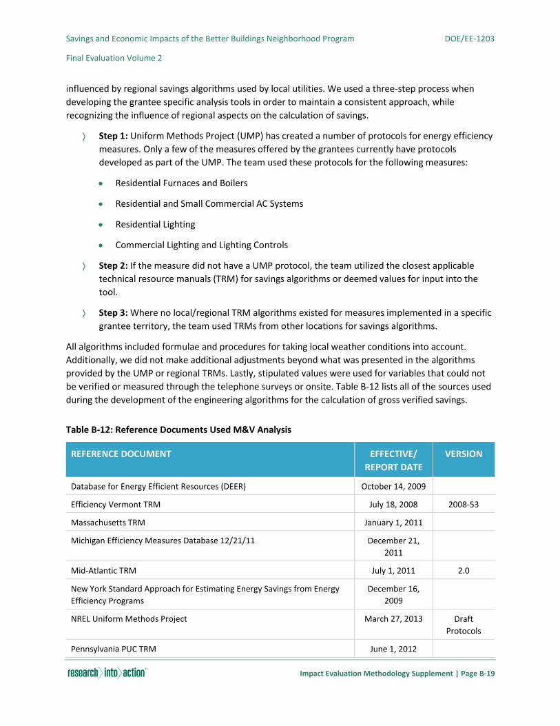
Savings and Economic Impacts of the Better Buildings Neighborhood Program DOE/EE-1203
Final Evaluation Volume 2
Impact Evaluation Methodology Supplement | Page B-19
influenced by regional savings algorithms used by local utilities. We used a three-step process when
developing the grantee specific analysis tools in order to maintain a consistent approach, while
recognizing the influence of regional aspects on the calculation of savings.
Step 1: Uniform Methods Project (UMP) has created a number of protocols for energy efficiency
measures. Only a few of the measures offered by the grantees currently have protocols
developed as part of the UMP. The team used these protocols for the following measures:
Residential Furnaces and Boilers
Residential and Small Commercial AC Systems
Residential Lighting
Commercial Lighting and Lighting Controls
Step 2: If the measure did not have a UMP protocol, the team utilized the closest applicable
technical resource manuals (TRM) for savings algorithms or deemed values for input into the
tool.
Step 3: Where no local/regional TRM algorithms existed for measures implemented in a specific
grantee territory, the team used TRMs from other locations for savings algorithms.
All algorithms included formulae and procedures for taking local weather conditions into account.
Additionally, we did not make additional adjustments beyond what was presented in the algorithms
provided by the UMP or regional TRMs. Lastly, stipulated values were used for variables that could not
be verified or measured through the telephone surveys or onsite. Table B-12 lists all of the sources used
during the development of the engineering algorithms for the calculation of gross verified savings.
Table B-12: Reference Documents Used M&V Analysis
REFERENCE DOCUMENT EFFECTIVE/
REPORT DATE
VERSION
Database for Energy Efficient Resources (DEER) October 14, 2009
Efficiency Vermont TRM July 18, 2008 2008-53
Massachusetts TRM January 1, 2011
Michigan Efficiency Measures Database 12/21/11 December 21,
2011
Mid-Atlantic TRM July 1, 2011 2.0
New York Standard Approach for Estimating Energy Savings from Energy
Efficiency Programs
December 16,
2009
NREL Uniform Methods Project March 27, 2013 Draft
Protocols
Pennsylvania PUC TRM June 1, 2012

Savings and Economic Impacts of the Better Buildings Neighborhood Program DOE/EE-1203
Final Evaluation Volume 2
Impact Evaluation Methodology Supplement | Page B-20
REFERENCE DOCUMENT EFFECTIVE/
REPORT DATE
VERSION
State of Illinois Energy Efficiency TRM June 1, 2012
Continued…
State of Ohio Energy Efficiency TRM August 6, 2010
Tennessee Valley Authority Measurement Manual July 14, 2010
Texas Deemed Savings Installation and Efficiency Standards April 1, 2010
United Illuminating and Connecticut Light and Power Program Savings
Documentation
September 21,
2010
Wisconsin Business Programs: Deemed Savings Manual March 22, 2010 1.0
We applied data collected from our sampled desk reviews, phone surveys (in the case of the preliminary
evaluation), and site visits to these various analysis tools. In the event we observed a discrepancy
between site visit documentation and project documentation reviewed during the desk review, we
deferred to the site visit data for our analysis.
There were a variety of fuel types that we encountered during the review of project savings. The M&V
efforts addressed all fuel types including electric, natural gas, fuel oil, propane, and others. However,
based on results from the preliminary evaluation, the team found that reporting of less common fuel
types such as fuel oil and propane was very inconsistent and led to erroneous analysis findings for these
fuel types. As a result, analysis was only performed on reported energy savings expressed in millions of
BTUs (MMBtu), electricity kilowatt-hours (kWh) and natural gas therms. Energy savings analyzed based
on project documentation and/or onsite visits by the evaluation team are ultimately expressed in
MMBtu for consistency and for comparison with DOE reporting protocols. The conversion factors are
located in Appendix K.
B.4. BILLING REGRESSION METHODS
A billing regression analysis approach was utilized for those instances when sufficient customer billing
data and participant tracking data (for example, information on when measures were installed) were
available. The billing regression model utilizes data on monthly electricity or natural gas consumption
before and after program participation. To accomplish this, we reviewed all grantee data to determine
which grantees had provided sufficient billing data to support a model. Based on this review, only 19
grantees had adequate billing data for the modeling task.
All model results are discussed in more detail in the Billing regression analysis Results section.
Savings and Economic Impacts of the Better Buildings Neighborhood Program DOE/EE-1203
Final Evaluation Volume 2
Impact Evaluation Methodology Supplement | Page B-21
B.4.1. MODEL SPECIFICATIONS
Final Model Specification
For our general model, we developed a fixed effects billing regression model specification.46 One of the
principal advantages of using the billing regression model is that it theoretically allows for the
consideration of confounding factors, such as customer size, geographic location, and changes in the
features of the building between the pre- and post-participation months. Though some measure and
household details were included in the grantee quarterly submissions, the data were often inconsistent
and introduced added uncertainty. The final model specification selected is a simplified model that relies
on fewer variables to control for external factors that might affect energy consumption; however, this
specification produces savings estimates quite similar to those found in the more complex
specifications. In addition to weather and measure variables, the billing model specification relied on
dummy variables for month (to control for possible seasonal influences beyond weather) and customer-
specific dummy variables to control for all other influences that may be affecting energy consumption at
the customer level.
As discussed elsewhere in this report, the billing regression analysis uses a baseline of pre-project
existing conditions at the site. This approach may differ from the M&V analysis where building code is
used as the baseline if actual baseline conditions cannot be verified during onsite inspections or from
supporting project documentation. As a consequence of this difference in methodology, the savings
estimates generated by the two approaches are not fully comparable.
The fixed effects model specification for residential participants with electricity billing data is as follows:
Where:
kWhi,t = Normalized kWh usage in month t for customer i
Posti,t = Binary variable indicating post-participation month for customer i
Weathert = Weather data for month t (heating degree-days [HDD] and cooling degree-days
[CDD])
Montht = Set of binary variables indicating whether or not billing month t is January,
February, March, April, etc.
αi = Customer-specific constant
46 The fixed effects model is a model specification that incorporates non-random, time-invariant explanatory variables in the
traditional multi-variate regression framework. These constant terms help control for possible influences relating to individual
cohorts and time periods that are not controlled for explicitly in the available data. By controlling for these influences using
these additional constant terms, the fixed effects model provides a more robust estimation of changes in energy use over time.
kWhi,t =ai + b1(Posti,t )+ b2 (Weathert )+ b j (Montht )+ej=3
13
å

Savings and Economic Impacts of the Better Buildings Neighborhood Program DOE/EE-1203
Final Evaluation Volume 2
Impact Evaluation Methodology Supplement | Page B-22
Similarly, an analogous model was developed for those program participants with natural gas
consumption data:
Where:
Thermsi,t = Normalized natural gas usage in month t for customer i
Posti,t = Binary variable indicating post-participation month for customer i
Weathert = Weather data for month t (HDD)
Montht = Set of binary variables indicating whether or not billing month t is January,
February, March, etc.
αi = Customer-specific constant
Before the data were used in the model, both the electricity and gas data were subjected to a data
cleaning process that screened out participants with insufficient pre-retrofit or post-retrofit data, and
unusually small or large fuel consumption data. These data screens helped to eliminate outlier values
that would have otherwise biased the model results. Our team tried a variety of data screens, all
resulting in similar model savings estimates. Accordingly, we believe that our final data screens do not
bias the results even though a significant amount of observations were omitted. Additional detail on
these screens is provided in the section B.4.2 below.
Alternate Model Specifications
The team also ran a series of alternate model specifications to confirm that the results did not change
substantially. Details on the specifications tried and the corresponding output can be found in Appendix
G.
B.4.2. DATA CLEANING Once all data were received from the grantees, our team developed data screens to clean the billing
data for analysis. It was important to remove any potentially erroneous billing data from the final
modeling dataset to avoid biasing the estimation results.
The screens used to produce the final electricity dataset for modeling removed the following:
Observations with monthly electricity consumption less than or equal to 100 kWh
Observations with monthly electricity consumption greater than 10,000 kWh
Observations with a billing period less than 28 days
Observations with a billing period greater than 35 days
Households with a pre-retrofit billing period less than 12 months
Thermsi,t =ai + b1(Posti,t )+ b2 (Weathert )+ b j (Montht )+ej=3
13
å

Savings and Economic Impacts of the Better Buildings Neighborhood Program DOE/EE-1203
Final Evaluation Volume 2
Impact Evaluation Methodology Supplement | Page B-23
Households with a post-retrofit billing period less than 12 months
Households with average pre-retrofit monthly electricity consumption the less than or equal to
200 kWh
Households with average pre-retrofit monthly electricity consumption greater than 5,000 kWh
Households whose average monthly electricity consumption in the post-retrofit billing period
was more than double the average consumption in the pre-retrofit billing period
Households with no installed electricity savings listed in the program tracking data
Similarly, the screening process for the gas dataset removed the following:
Observations with monthly electricity consumption less than or equal to 5 therms
Observations with monthly electricity consumption greater than 300 therms
Observations with a billing period less than 28 days
Observations with a billing period greater than 35 days
Households with average pre-retrofit billing period less than 12 months
Households with a post-retrofit billing period less than 12 months
Households with average pre-retrofit monthly natural gas consumption less than or equal to 20
therms
Households with average pre-retrofit monthly natural gas consumption greater than 250 therms
Households whose average monthly natural gas consumption in the post-retrofit billing period
was more than double the average consumption in the pre-retrofit billing period
Households with no installed natural gas savings listed in the program tracking data
A summary of these data screens is shown in Table B-13. Though a variety of data screens were tried on
the models as a sensitivity test, none altered the results or statistical significance of the results greatly,
so we opted to use the data screens listed above, even though they screened out 70-80% of the cases.
Details on some of the alternate data screens we tried and their impact on the regression output can be
found in Appendix E.
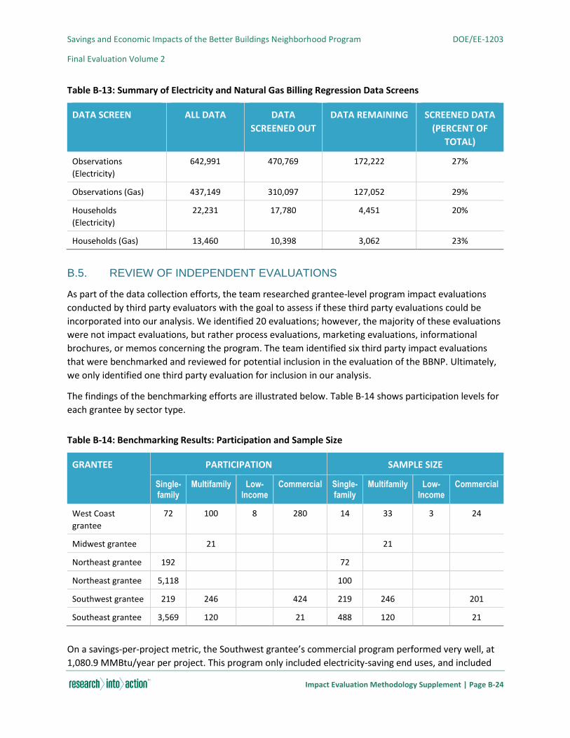
Savings and Economic Impacts of the Better Buildings Neighborhood Program DOE/EE-1203
Final Evaluation Volume 2
Impact Evaluation Methodology Supplement | Page B-24
Table B-13: Summary of Electricity and Natural Gas Billing Regression Data Screens
DATA SCREEN ALL DATA DATA
SCREENED OUT
DATA REMAINING SCREENED DATA
(PERCENT OF
TOTAL)
Observations
(Electricity)
642,991 470,769 172,222 27%
Observations (Gas) 437,149 310,097 127,052 29%
Households
(Electricity)
22,231 17,780 4,451 20%
Households (Gas) 13,460 10,398 3,062 23%
B.5. REVIEW OF INDEPENDENT EVALUATIONS
As part of the data collection efforts, the team researched grantee-level program impact evaluations
conducted by third party evaluators with the goal to assess if these third party evaluations could be
incorporated into our analysis. We identified 20 evaluations; however, the majority of these evaluations
were not impact evaluations, but rather process evaluations, marketing evaluations, informational
brochures, or memos concerning the program. The team identified six third party impact evaluations
that were benchmarked and reviewed for potential inclusion in the evaluation of the BBNP. Ultimately,
we only identified one third party evaluation for inclusion in our analysis.
The findings of the benchmarking efforts are illustrated below. Table B-14 shows participation levels for
each grantee by sector type.
Table B-14: Benchmarking Results: Participation and Sample Size
GRANTEE PARTICIPATION SAMPLE SIZE
Single-family
Multifamily Low-Income
Commercial Single-family
Multifamily Low-Income
Commercial
West Coast
grantee
72 100 8 280 14 33 3 24
Midwest grantee 21 21
Northeast grantee 192 72
Northeast grantee 5,118 100
Southwest grantee 219 246 424 219 246 201
Southeast grantee 3,569 120 21 488 120 21
On a savings-per-project metric, the Southwest grantee’s commercial program performed very well, at
1,080.9 MMBtu/year per project. This program only included electricity-saving end uses, and included
Savings and Economic Impacts of the Better Buildings Neighborhood Program DOE/EE-1203
Final Evaluation Volume 2
Impact Evaluation Methodology Supplement | Page B-25
commercial lighting and commercial HVAC measures. The Midwest grantee also did very well, at 856.2
MMBtu/year per project. The Midwest grantee only worked with gas-saving end-uses and included
replacing heating units, installing air sealing measures, altering hot water distribution systems, and
adding insulation to the roof cavity. These projects only included multifamily buildings, which accounts
for the high savings value. The West Coast grantee had a low energy savings per project value, which can
be explained by the fact that their commercial programs only included small commercial buildings, and
the program only included electricity-saving end-uses, all of which would be residential-sized, not
industrial-sized units. All remaining grantees measured gas and electricity savings, with the Northeast
grantee’s direct install incorporating fuel oil, wood, propane, coal, kerosene, and pellets as part of the
program. Table B-15 shows total gross savings and savings per project by grantee.
Table B-15: Benchmarking Results: Gross Savings and Savings per Project
GRANTEE GROSS SAVINGS (MMBtu) SAVINGS PER PROJECT (MMBtu)
Single-family
Multifamily Low-Income
Commercial Single-family
Multifamily Low-Income
Commercial
West Coast
grantee
1,037 428 13.4 492.6 14.4 4.3 1.7 1.8
Midwest grantee 17,980 856.2
Northeast grantee 10,445 54.4
Northeast grantee 47,156 9.2
Southwest grantee 2,351 458,318.80 10.7 1080.9
Southeast grantee 28,841 8,420 10,140.60 8.1 70.2 482.9
Each evaluator had preferred methods of measuring program energy savings. The West Coast grantee
was evaluated by use of desk reviews only. The evaluators for the Southwest and Northeast grantees
utilized billing regression analysis and desk reviews, while the evaluators for the Southeast grantee
utilized a combination of billing regression analysis, desk reviews, and energy modeling to estimate
savings. Table B-16 shows the methods used to determine energy savings by grantee.
Table B-16: Benchmarking Results: Methods Used to Determine Energy Savings
GRANTEE METHODS USED
Billing Regression Analysis Desk Reviews Energy Modeling
West Coast grantee x
Midwest grantee x
Northeast grantee x x
Northeast grantee x
Savings and Economic Impacts of the Better Buildings Neighborhood Program DOE/EE-1203
Final Evaluation Volume 2
Impact Evaluation Methodology Supplement | Page B-26
Southwest grantee x x
Southeast grantee x x x
Only two evaluations reported realization rates. The evaluator for the Northeast grantee reported a 78%
realization rate. The Southeast grantee’s evaluator reported 65.9% realization rate for single-family, and
chose to apply a 100% realization rate to both commercial and multifamily due to the lack of required
documentation to conduct the analyses.
B.6. NET-TO-GROSS METHODOLOGY
We conducted surveys to provide inputs to the NTG calculations with two groups: participating end
users and participating and nonparticipating contractors. The final NTG estimate for the residential
sector is based on both end user- and contractor-derived NTG estimates; participating end user free-
ridership informs the lower bound NTG estimates (that is, NTG with free-ridership), and contractor-
derived estimates of free-ridership and spillover inform the upper bound NTG estimates (that is, NTG
with free-ridership and spillover) (Table B-17). The final NTG estimates for the commercial and
multifamily sector are derived solely from participating end user free-ridership. The final residential NTG
value is the mid-point between the end user- and contractor-derived NTG estimates. While there are
some indications of spillover from the commercial grantees, the sample size of surveyed contractors is
too small to develop a reliable estimate.
Table B-17: Net-to-Gross Ratio Calculation Methods
SECTOR LOWER BOUND NTG
ESTIMATES DERIVED FROM
PARTICIPATING END USERS
(FREE-RIDERSHIP ONLY)
UPPER BOUND NTG ESTIMATES
DERIVED FROM PARTICIPATING
AND NONPARTICIPATING
CONTRACTORS (FREE-RIDERSHIP
AND SPILLOVER)
FINAL
NET-TO-GROSS
RATIO
Residential 0.78 1.10 0.94
Commercial 0.85 Not estimated 0.85
Multifamily 0.99 Not estimated 0.99
B.6.1. LOWER BOUND NET-TO-GROSS RATIO ESTIMATES DERIVED FROM PARTICIPATING END USERS
Overview
Sampled commercial end users were those that completed an onsite verification survey as part of the
M&V activities for the final evaluation; the onsite verification survey included the NTG questions. We
sampled multifamily end users from a desk review and conducted the NTG survey over the phone.
Sampled residential end users were those that completed an online survey that included process and
NTG questions. Our end user survey questions sought information relating both to program influence
(free-ridership) and spillover; however, we are able to provide numeric estimates of free-ridership only.

Savings and Economic Impacts of the Better Buildings Neighborhood Program DOE/EE-1203
Final Evaluation Volume 2
Impact Evaluation Methodology Supplement | Page B-27
(Our study methodology did not include estimation of energy savings associated with respondents’
reported spillover activity, nor with verifying the spillover.) Instead we gathered spillover estimates from
participating and nonparticipating contractors (see following sub-section). We compiled the free-
ridership results for each project from two components, what the participant would likely have done in
the absence of the program and the influence the participant states that the program had on the
upgrade actions taken. For commercial and multifamily sectors (which were based on the M&V sample),
we rolled up the per-project results to the stratum level within each sector. We multiplied the stratum-
average free-ridership score by the stratum verified savings and summed the resulting stratum-net-
savings to obtain a sector net savings. We calculated sector NTG as the ratio of the sector-net-savings
divided by the sector-verified-savings. Residential lower bound NTG was not based on M&V sampling,
and thus did not have case weights tied to verified savings. Residential lower bound NTG was weighted
in a similar fashion, but using a grantee-level weight (instead of stratum verified savings); grantee-
stratum weights were developed by multiplying the ratio of a grantee’s total project count to total BBNP
project count by the ratio of respondents in the grantee’s stratum to total survey respondents.
Additional Methodological Details
We used the survey method (equivalently, the self-report method) for the same reasons that have made
it the most common method supporting NTG analyses: there are few other methods available and, as is
typical, these methods are not appropriate for the program design or the available evaluation
resources.47 According to Haeri and Khawaja (2002), “self-report remains the most common method for
determining free-ridership,” in spite of the fact that many researchers engaged in estimating NTG have
significant concerns with the methodology.48
Free-ridership (FR) was first calculated at the record level: each record received a free-ridership score
ranging from 0-1 (where 0 means no free-ridership, and 1 means 100% free-ridership; thus, .6 means
60% free-ridership). The 0-1 FR range means someone could be a total free-rider (a value of 1), a partial
free-rider (0.01-0.99) or not a free-rider (0). FR values consist of two components, change and influence,
each of equal weight (and thus scored a value ranging from 0-.5).
The change component indicates what the participant would have likely done if the program had not
incented them to do the upgrades, and assigns a FR change score (ranging from 0-0.5), depending on
what the respondent indicates they would have done in absence of the program. The following list
exhibits the options that respondents were able to choose from (regarding FR change), and the
corresponding FR change value is listed in parentheses following each option:
1. Would they have done the upgrades anyway and paid the full cost themselves? (.5)
2. Would they have done some or different efficient upgrades, that would ultimately result in less
savings than they achieved through the program? (.25)
47 These methods are experimental design and quasi-experimental design.
48 Haeriand and Khawaja, 2012 cite a TecMarket Works, 2006 which states, “the issues of identifying free-riders are complicated
and estimating reliable program-specific free-ridership is problematic at best.”
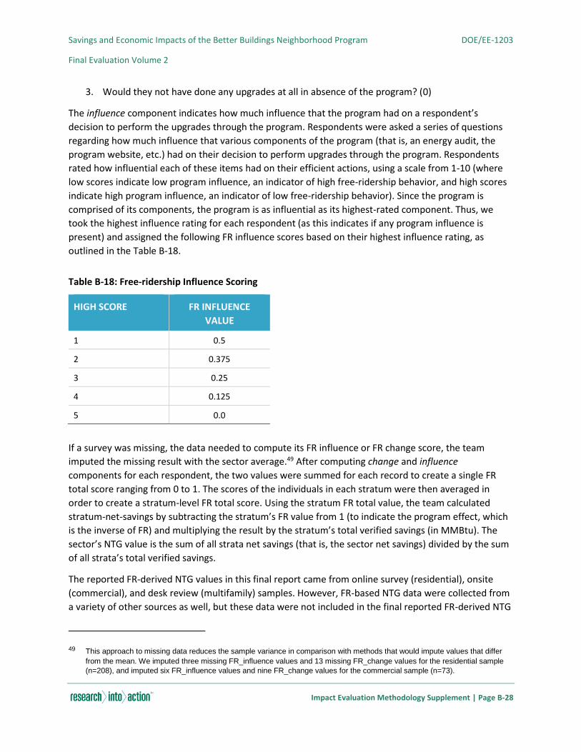
Savings and Economic Impacts of the Better Buildings Neighborhood Program DOE/EE-1203
Final Evaluation Volume 2
Impact Evaluation Methodology Supplement | Page B-28
3. Would they not have done any upgrades at all in absence of the program? (0)
The influence component indicates how much influence that the program had on a respondent’s
decision to perform the upgrades through the program. Respondents were asked a series of questions
regarding how much influence that various components of the program (that is, an energy audit, the
program website, etc.) had on their decision to perform upgrades through the program. Respondents
rated how influential each of these items had on their efficient actions, using a scale from 1-10 (where
low scores indicate low program influence, an indicator of high free-ridership behavior, and high scores
indicate high program influence, an indicator of low free-ridership behavior). Since the program is
comprised of its components, the program is as influential as its highest-rated component. Thus, we
took the highest influence rating for each respondent (as this indicates if any program influence is
present) and assigned the following FR influence scores based on their highest influence rating, as
outlined in the Table B-18.
Table B-18: Free-ridership Influence Scoring
HIGH SCORE FR INFLUENCE
VALUE
1 0.5
2 0.375
3 0.25
4 0.125
5 0.0
If a survey was missing, the data needed to compute its FR influence or FR change score, the team
imputed the missing result with the sector average.49 After computing change and influence
components for each respondent, the two values were summed for each record to create a single FR
total score ranging from 0 to 1. The scores of the individuals in each stratum were then averaged in
order to create a stratum-level FR total score. Using the stratum FR total value, the team calculated
stratum-net-savings by subtracting the stratum’s FR value from 1 (to indicate the program effect, which
is the inverse of FR) and multiplying the result by the stratum’s total verified savings (in MMBtu). The
sector’s NTG value is the sum of all strata net savings (that is, the sector net savings) divided by the sum
of all strata’s total verified savings.
The reported FR-derived NTG values in this final report came from online survey (residential), onsite
(commercial), and desk review (multifamily) samples. However, FR-based NTG data were collected from
a variety of other sources as well, but these data were not included in the final reported FR-derived NTG
49 This approach to missing data reduces the sample variance in comparison with methods that would impute values that differ
from the mean. We imputed three missing FR_influence values and 13 missing FR_change values for the residential sample
(n=208), and imputed six FR_influence values and nine FR_change values for the commercial sample (n=73).
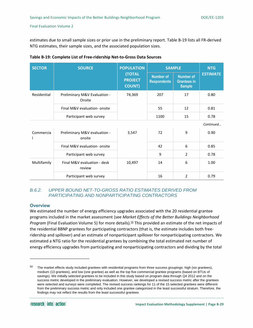
Savings and Economic Impacts of the Better Buildings Neighborhood Program DOE/EE-1203
Final Evaluation Volume 2
Impact Evaluation Methodology Supplement | Page B-29
estimates due to small sample sizes or prior use in the preliminary report. Table B-19 lists all FR-derived
NTG estimates, their sample sizes, and the associated population sizes.
Table B-19: Complete List of Free-ridership Net-to-Gross Data Sources
SECTOR SOURCE POPULATION
(TOTAL
PROJECT
COUNT)
SAMPLE NTG
ESTIMATE Number of
Respondents Number of Grantees in
Sample
Residential Preliminary M&V Evaluation -
Onsite
74,369 207 17 0.80
Final M&V evaluation- onsite 55 12 0.81
Participant web survey 1100 15 0.78
Continued…
Commercia
l
Preliminary M&V evaluation -
onsite
3,547 72 9 0.90
Final M&V evaluation- onsite 42 6 0.85
Participant web survey 9 2 0.78
Multifamily Final M&V evaluation - desk
review
10,497 14 6 1.00
Participant web survey 16 2 0.79
B.6.2. UPPER BOUND NET-TO-GROSS RATIO ESTIMATES DERIVED FROM PARTICIPATING AND NONPARTICIPATING CONTRACTORS
Overview
We estimated the number of energy efficiency upgrades associated with the 20 residential grantee
programs included in the market assessment (see Market Effects of the Better Buildings Neighborhood
Program (Final Evaluation Volume 5) for more details).50 This provided an estimate of the net impacts of
the residential BBNP grantees for participating contractors (that is, the estimate includes both free-
ridership and spillover) and an estimate of nonparticipant spillover for nonparticipating contractors. We
estimated a NTG ratio for the residential grantees by combining the total estimated net number of
energy efficiency upgrades from participating and nonparticipating contractors and dividing by the total
50 The market effects study included grantees with residential programs from three success groupings: high (six grantees),
medium (13 grantees), and low (one grantee) as well as the top five commercial grantee programs (based on BTUs of
savings). We initially selected grantees to be included in this study based on program data through Q4 2012 and on the
success metric developed in the preliminary evaluation. However, we developed a revised success metric after the grantees
were selected and surveys were completed. The revised success rankings for 11 of the 15 selected grantees were different
from the preliminary success metric and only included one grantee categorized in the least successful stratum. Therefore, the
findings may not reflect the results from the least successful grantees
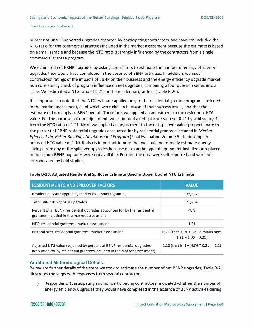
Savings and Economic Impacts of the Better Buildings Neighborhood Program DOE/EE-1203
Final Evaluation Volume 2
Impact Evaluation Methodology Supplement | Page B-30
number of BBNP-supported upgrades reported by participating contractors. We have not included the
NTG ratio for the commercial grantees included in the market assessment because the estimate is based
on a small sample and because the NTG ratio is strongly influenced by the contractors from a single
commercial grantee program.
We estimated net BBNP upgrades by asking contractors to estimate the number of energy efficiency
upgrades they would have completed in the absence of BBNP activities. In addition, we used
contractors’ ratings of the impacts of BBNP on their business and the energy efficiency upgrade market
as a consistency check of program influence on net upgrades, combining a four question series into a
scale. We estimated a NTG ratio of 1.21 for the residential grantees (Table B-20).
It is important to note that the NTG estimate applied only to the residential grantee programs included
in the market assessment, all of which were chosen because of their success levels, and that the
estimate did not apply to BBNP overall. Therefore, we applied an adjustment to the residential NTG
value. For the purposes of our adjustment, we estimated a net spillover value of 0.21 by subtracting 1
from the NTG ratio of 1.21. Next, we applied an adjustment to the net spillover value proportionate to
the percent of BBNP residential upgrades accounted for by residential grantees included in Market
Effects of the Better Buildings Neighborhood Program (Final Evaluation Volume 5), to develop an
adjusted NTG value of 1.10. It also is important to note that we could not directly estimate energy
savings from any of the spillover upgrades because data on the type of equipment installed or replaced
in these non-BBNP upgrades were not available. Further, the data were self-reported and were not
corroborated by field studies.
Table B-20: Adjusted Residential Spillover Estimate Used in Upper Bound NTG Estimate
RESIDENTIAL NTG AND SPILLOVER FACTORS VALUE
Residential BBNP upgrades, market assessment grantees 35,297
Total BBNP Residential upgrades 73,704
Percent of all BBNP residential upgrades accounted for by the residential
grantees included in the market assessment
48%
NTG, residential grantees, market assessment 1.21
Net spillover, residential grantees, market assessment 0.21 (that is, NTG value minus one:
1.21 – 1.00 = 0.21)
Adjusted NTG value (adjusted by percent of BBNP residential upgrades
accounted for by residential grantees included in the market assessment)
1.10 (that is, 1+ (48% * 0.21) = 1.1)
Additional Methodological Details Below are further details of the steps we took to estimate the number of net BBNP upgrades; Table B-21
illustrates the steps with responses from several contractors.
Respondents (participating and nonparticipating contractors) indicated whether the number of
energy efficiency upgrades they would have completed in the absence of BBNP activities during
Savings and Economic Impacts of the Better Buildings Neighborhood Program DOE/EE-1203
Final Evaluation Volume 2
Impact Evaluation Methodology Supplement | Page B-31
the 2010-2013 period, with all other things remaining the same (that is, the economy, energy
prices, and other energy efficiency programs), would have been higher, lower, or the same.
If respondents thought the number of upgrades would have been higher in absence of the
program, we asked them to estimate the percentage higher. If they thought the number of
upgrades would have been lower, we asked them to estimate the percentage of the total
number of upgrades that they would have completed during this period. From those estimates,
we estimated the number of upgrades that the respondent would have conducted in absence of
the program.51 See column C in Table B-21.
Subtracting this value from a respondent’s estimate of total upgrades performed between 2010
and 2013 (column A) provides an initial estimate of the net impacts of BBNP for participating
contractors (that is, the estimate includes both free-ridership and spillover) and an estimate of
nonparticipant spillover for nonparticipating contractors (column D).
For example, respondent 1 completed 160 upgrades between 2010 and 2013 (column A) and
estimated that he/she would have completed 128 upgrades in the absence of the BBNP grantee
(column C); we estimated a net impact of 32 upgrades for the respondent (column D & J). The
same respondent completed five upgrades with BBNP, resulting in an estimated NTG ratio of 6.4
for the respondent (that is, 32 divided by five = 6.4; column K), meaning that the BBNP grantee
program resulted in spillover upgrades for the respondent. Respondent 2 had an NTG value of
less than one. The respondent estimated 1,080 upgrades in the absence of the BBNP grantee –
or 2,520 net upgrades – but completed 3,000 upgrades with the grantee, resulting in an
estimated NTG of 0.84 (that is, 2,520 divided by 3,000 = 0.84).
Next, we used respondents’ ratings of the impacts of BBNP on their business and the energy
efficiency upgrade market as a consistency check of program influence on net upgrades. We
combined the four question series (footnoted in Table B-21) into a scale and used an average
score of seven or higher (that is, rating BBNP as having a positive impact on their business and
the upgrade market) as the minimum required score to use a respondent’s estimate of net
impacts (column I).52 Nonparticipating contractors, such as respondent 7, with a score below
seven received NTG ratios of 0.0 (that is, zero nonparticipant spillover upgrades):
A rating of seven or higher = 100% net (that is, the program had a strong impact on their
business, all BBNP projects are counted as net upgrades). For example, respondent 1.
51 Sixteen participating contractors and 123 non-participating contractors were unable to estimate the total number of upgrades
that they had conducted from 2010 to 2013. Eleven of these respondents (eight participating contactors and three non-
participating contractors) were able to estimate a percentage change in absence of the program. We estimated the total
number of upgrades for these 11 respondents in order to estimate net upgrades. We found that the respondents who were able
to estimate total upgrades had, on average, conducted 53 upgrades per FTE on average. To estimate the total upgrades for
the 11 respondents, we multiplied the number of FTEs that they had reported by 53. The remaining 128 respondents were
treated as zero values for the net upgrades analysis.
52 The four-question scale has a Cronbach’s α of 0.90. Cronbach’s α is a measure of inter-item correlation and scale reliability. A
score of 0.9 or higher is generally considered an excellent indication of inter-item correlation and scale reliability (DeVellis,
1991).
Savings and Economic Impacts of the Better Buildings Neighborhood Program DOE/EE-1203
Final Evaluation Volume 2
Impact Evaluation Methodology Supplement | Page B-32
A rating of six = 80% net (that is, 80% of BBNP projects are counted as net upgrades).
A rating of five = 60% net. For example, respondent 8.
A rating of four = 40% net.
A rating of three = 20% net.
A rating of two or lower = 0% net (that is, strong disagreement that BBNP had a positive
effect on their business; none of the BBNP projects are counted as net upgrades).
We applied this rule similarly to participating contractors who said that there would have been
no change in absence of the program. These respondents had initial net upgrade values of 0;
however, if they gave positive ratings to BBNP, we proportionally assigned them percentages of
BBNP program upgrades.
For participating contractors identifying negative market effects (that is, they would have
completed more projects without BBNP), we inversely applied a similar rule based on the
respondents’ agreement with the impact of BBNP on their business.53 For example, respondent
5 below indicated that he/she would have conducted 480 upgrades in absence of the program
and had conducted 400 in total, resulting in an initial net upgrade value of -80. This respondent
then gave an average rating of three to the scale questions and, in particular, gave a rating
greater than two to the statement “There is more business for your company than there would
have been without the program,” showing a slight positive impact of the program. We assigned
this respondent 80% of the negative net upgrades, increasing the final net upgrade value to -64
(80% of -80 = -64).
Last, for participating contractors, we examined the ratio of net BBNP upgrades to the number
of upgrades completed with BBNP (that is, individual NTG ratios) to identify any outliers. Four
participants had NTG ratios more than three standard deviations above or below the mean NTG
ratio. Three outlier respondents estimated that, for every one BBNP upgrade, they had
completed 60 or more additional upgrades as a result of the program. We replaced their
estimates of net upgrades with their estimated number of BBNP upgrades.54 For example,
respondent 6 in had completed 650 total upgrades from 2010 to 2013, four of which were BBNP
upgrades, and estimated that he/she would have completed only 98 upgrades in absence of the
program, resulting in an initial NTG ratio of 138 (552 divided by four). We assigned a net
upgrade value to this respondent equal to the number of BBNP upgrades that he/she
completed, resulting in an NTG value of 1.0.
53 The in-depth interviews examined why some contractors reported negative program effects. They described dynamics such as
BBNP unevenly promoting certain contractors over others, competing contractors utilizing subcontractors to get around BBNP
rules, BBNP drawing contractors to come from other geographic areas, and nonparticipating contractors leveraging program
opportunities.
54 These respondents had values over seven for the program influence scale, indicating strong BBNP influence.
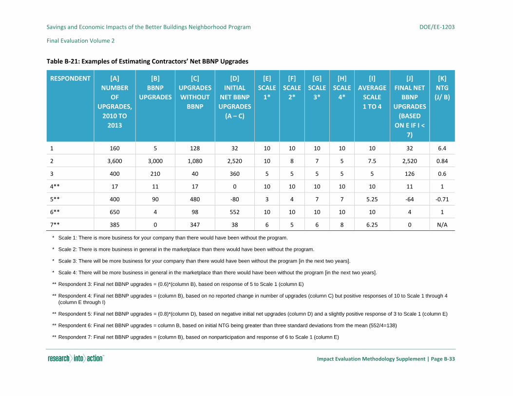
Savings and Economic Impacts of the Better Buildings Neighborhood Program DOE/EE-1203
Final Evaluation Volume 2
Impact Evaluation Methodology Supplement | Page B-33
Table B-21: Examples of Estimating Contractors’ Net BBNP Upgrades
RESPONDENT [A]
NUMBER
OF
UPGRADES,
2010 TO
2013
[B]
BBNP
UPGRADES
[C]
UPGRADES
WITHOUT
BBNP
[D]
INITIAL
NET BBNP
UPGRADES
(A – C)
[E]
SCALE
1*
[F]
SCALE
2*
[G]
SCALE
3*
[H]
SCALE
4*
[I]
AVERAGE
SCALE
1 TO 4
[J]
FINAL NET
BBNP
UPGRADES
(BASED
ON E IF I <
7)
[K]
NTG
(J/ B)
1 160 5 128 32 10 10 10 10 10 32 6.4
2 3,600 3,000 1,080 2,520 10 8 7 5 7.5 2,520 0.84
3 400 210 40 360 5 5 5 5 5 126 0.6
4** 17 11 17 0 10 10 10 10 10 11 1
5** 400 90 480 -80 3 4 7 7 5.25 -64 -0.71
6** 650 4 98 552 10 10 10 10 10 4 1
7** 385 0 347 38 6 5 6 8 6.25 0 N/A
* Scale 1: There is more business for your company than there would have been without the program.
* Scale 2: There is more business in general in the marketplace than there would have been without the program.
* Scale 3: There will be more business for your company than there would have been without the program [in the next two years].
* Scale 4: There will be more business in general in the marketplace than there would have been without the program [in the next two years].
** Respondent 3: Final net BBNP upgrades = (0.6)*(column B), based on response of 5 to Scale 1 (column E)
** Respondent 4: Final net BBNP upgrades = (column B), based on no reported change in number of upgrades (column C) but positive responses of 10 to Scale 1 through 4
(column E through I)
** Respondent 5: Final net BBNP upgrades = (0.8)*(column D), based on negative initial net upgrades (column D) and a slightly positive response of 3 to Scale 1 (column E)
** Respondent 6: Final net BBNP upgrades = column B, based on initial NTG being greater than three standard deviations from the mean (552/4=138)
** Respondent 7: Final net BBNP upgrades = (column B), based on nonparticipation and response of 6 to Scale 1 (column E)

Savings and Economic Impacts of the Better Buildings Neighborhood Program DOE/EE-1203
Final Evaluation Volume 2
Impact Evaluation Methodology Supplement | Page B-34
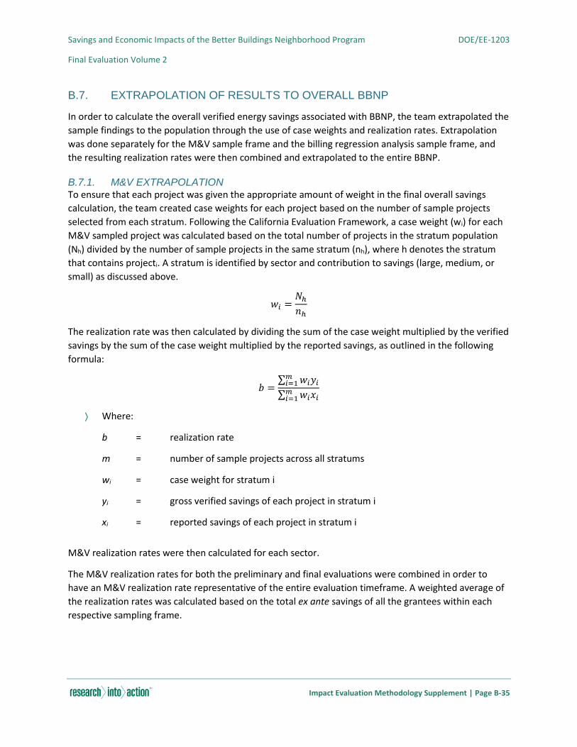
Savings and Economic Impacts of the Better Buildings Neighborhood Program DOE/EE-1203
Final Evaluation Volume 2
Impact Evaluation Methodology Supplement | Page B-35
B.7. EXTRAPOLATION OF RESULTS TO OVERALL BBNP
In order to calculate the overall verified energy savings associated with BBNP, the team extrapolated the
sample findings to the population through the use of case weights and realization rates. Extrapolation
was done separately for the M&V sample frame and the billing regression analysis sample frame, and
the resulting realization rates were then combined and extrapolated to the entire BBNP.
B.7.1. M&V EXTRAPOLATION To ensure that each project was given the appropriate amount of weight in the final overall savings
calculation, the team created case weights for each project based on the number of sample projects
selected from each stratum. Following the California Evaluation Framework, a case weight (wi) for each
M&V sampled project was calculated based on the total number of projects in the stratum population
(Nh) divided by the number of sample projects in the same stratum (nh), where h denotes the stratum
that contains projecti. A stratum is identified by sector and contribution to savings (large, medium, or
small) as discussed above.
𝑤𝑖 =𝑁ℎ
𝑛ℎ
The realization rate was then calculated by dividing the sum of the case weight multiplied by the verified
savings by the sum of the case weight multiplied by the reported savings, as outlined in the following
formula:
𝑏 =∑ 𝑤𝑖𝑦𝑖
𝑚𝑖=1
∑ 𝑤𝑖𝑥𝑖𝑚𝑖=1
Where:
b = realization rate
m = number of sample projects across all stratums
wi = case weight for stratum i
yi = gross verified savings of each project in stratum i
xi = reported savings of each project in stratum i
M&V realization rates were then calculated for each sector.
The M&V realization rates for both the preliminary and final evaluations were combined in order to
have an M&V realization rate representative of the entire evaluation timeframe. A weighted average of
the realization rates was calculated based on the total ex ante savings of all the grantees within each
respective sampling frame.
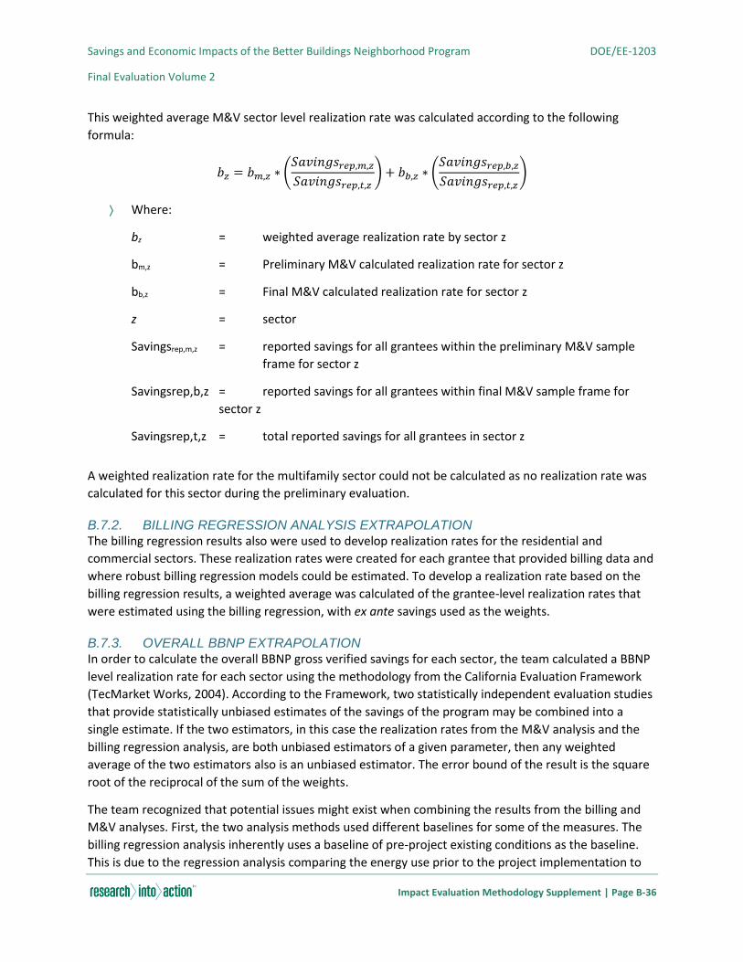
Savings and Economic Impacts of the Better Buildings Neighborhood Program DOE/EE-1203
Final Evaluation Volume 2
Impact Evaluation Methodology Supplement | Page B-36
This weighted average M&V sector level realization rate was calculated according to the following
formula:
𝑏𝑧 = 𝑏𝑚,𝑧 ∗ (𝑆𝑎𝑣𝑖𝑛𝑔𝑠𝑟𝑒𝑝,𝑚,𝑧
𝑆𝑎𝑣𝑖𝑛𝑔𝑠𝑟𝑒𝑝,𝑡,𝑧) + 𝑏𝑏,𝑧 ∗ (
𝑆𝑎𝑣𝑖𝑛𝑔𝑠𝑟𝑒𝑝,𝑏,𝑧
𝑆𝑎𝑣𝑖𝑛𝑔𝑠𝑟𝑒𝑝,𝑡,𝑧)
Where:
bz = weighted average realization rate by sector z
bm,z = Preliminary M&V calculated realization rate for sector z
bb,z = Final M&V calculated realization rate for sector z
z = sector
Savingsrep,m,z = reported savings for all grantees within the preliminary M&V sample
frame for sector z
Savingsrep,b,z = reported savings for all grantees within final M&V sample frame for
sector z
Savingsrep,t,z = total reported savings for all grantees in sector z
A weighted realization rate for the multifamily sector could not be calculated as no realization rate was
calculated for this sector during the preliminary evaluation.
B.7.2. BILLING REGRESSION ANALYSIS EXTRAPOLATION The billing regression results also were used to develop realization rates for the residential and
commercial sectors. These realization rates were created for each grantee that provided billing data and
where robust billing regression models could be estimated. To develop a realization rate based on the
billing regression results, a weighted average was calculated of the grantee-level realization rates that
were estimated using the billing regression, with ex ante savings used as the weights.
B.7.3. OVERALL BBNP EXTRAPOLATION In order to calculate the overall BBNP gross verified savings for each sector, the team calculated a BBNP
level realization rate for each sector using the methodology from the California Evaluation Framework
(TecMarket Works, 2004). According to the Framework, two statistically independent evaluation studies
that provide statistically unbiased estimates of the savings of the program may be combined into a
single estimate. If the two estimators, in this case the realization rates from the M&V analysis and the
billing regression analysis, are both unbiased estimators of a given parameter, then any weighted
average of the two estimators also is an unbiased estimator. The error bound of the result is the square
root of the reciprocal of the sum of the weights.
The team recognized that potential issues might exist when combining the results from the billing and
M&V analyses. First, the two analysis methods used different baselines for some of the measures. The
billing regression analysis inherently uses a baseline of pre-project existing conditions as the baseline.
This is due to the regression analysis comparing the energy use prior to the project implementation to
Savings and Economic Impacts of the Better Buildings Neighborhood Program DOE/EE-1203
Final Evaluation Volume 2
Impact Evaluation Methodology Supplement | Page B-37
the energy use after the project installation. However, the M&V analysis uses either a codes and
standards baseline or the pre-project existing conditions baseline depending on the measure installed
and the amount of information available for each measure. The second issue involves participant
spillover savings, which are energy savings due to measures installed by a program participant, likely
due to the influence of the program, but for which no program incentive was paid. The billing regression
analysis would capture from the savings due to participant spillover, while the M&V activities did not.
To address these concerns, we overlapped the M&V and billing regression analysis sample frames in an
effort to determine an adjustment factor that could account for these issues and allow the M&V and
billing analyses to be merged.
Adjustment Factor
For the final evaluation, the team overlapped sampled grantees between the M&V and billing regression
analysis sample frames. The intention of this overlap was to understand the differences on estimated
savings when using M&V versus billing regression, normalize those differences, and merge the M&V and
billing analyses to calculate an overall realization rate for the BBNP. After completion of the M&V and
billing regression activities, an overlap of 75 projects existing in both sample frames was examined. This
overlap presented an opportunity to corroborate the savings estimates of the two independent analysis
methods and to address some of the inherent differences between the M&V and billing regression
methodologies. Most notably:
Different baselines. In the case of the billing regression, the baseline is the pre-existing
conditions at the site, which may be less efficient than a building code baseline. In contrast, the
savings estimates used for the M&V analysis first assumed the actual baseline identified during
the verification exercise, and if this information is unavailable, building code was used. This is
generally more efficient than the existing equipment baseline.
Spillover savings. Spillover savings are energy savings due to measures installed by a program
participant, likely due to the influence of the program, but for which no program incentive was
paid. The billing regression analysis captures savings due to participant spillover, while the M&V
activities do not.
Other factors. The billing regression analysis captures the effect of outside factors that impact
energy savings, such as changes in occupancy, changes in usage patterns, interactive effects,
etc., but the M&V analysis generally does not account for these factors.
Adjustment Factor Methodology and Results We used a regression model to estimate a correction factor that can be used to adjust for the
aforementioned differences between the M&V and billing regression impact estimation results. This
regression relied on monthly consumption data (either electricity or natural gas) before and after
program participation, as well as weather information, and M&V verified savings estimates.
The model specification for participants with electricity billing data is as follows:
∆𝑘𝑊ℎ𝑖 = 𝑉𝑒𝑟𝑖𝑓𝑆𝑎𝑣𝑖 + ∆𝐻𝐷𝐷𝑖 + ∆𝐶𝐷𝐷𝑖 + 𝜀𝑖
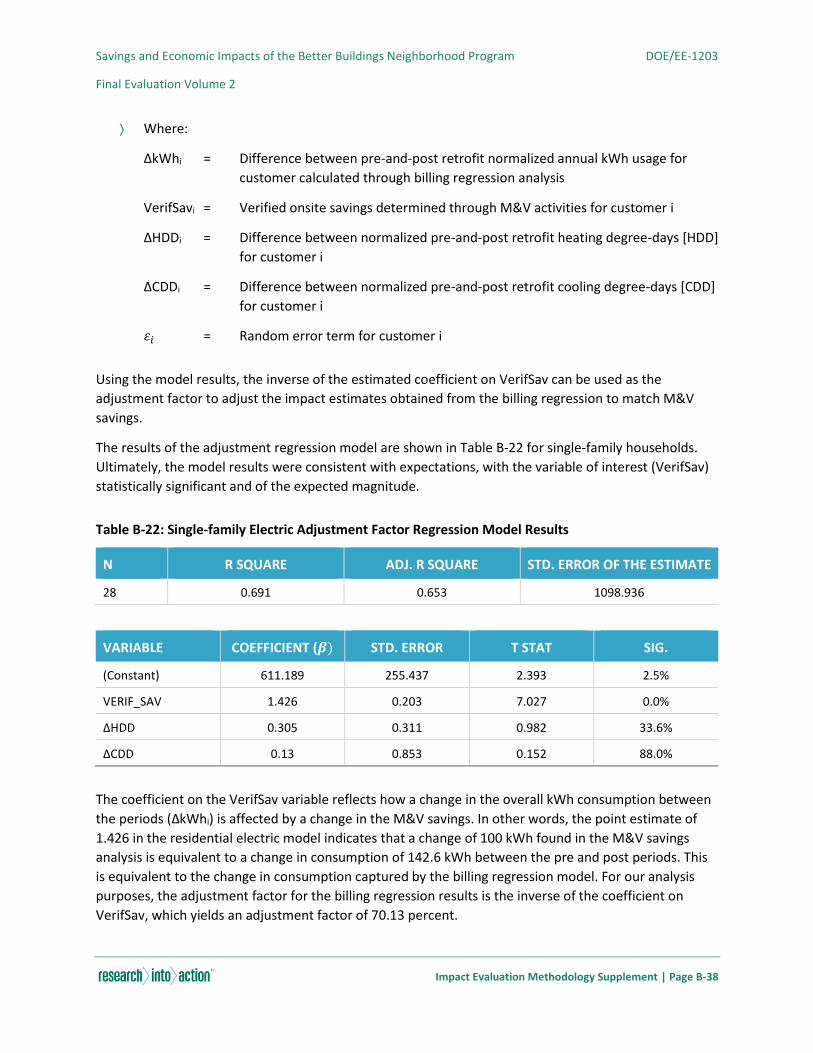
Savings and Economic Impacts of the Better Buildings Neighborhood Program DOE/EE-1203
Final Evaluation Volume 2
Impact Evaluation Methodology Supplement | Page B-38
Where:
ΔkWhi = Difference between pre-and-post retrofit normalized annual kWh usage for
customer calculated through billing regression analysis
VerifSavi = Verified onsite savings determined through M&V activities for customer i
ΔHDDi = Difference between normalized pre-and-post retrofit heating degree-days [HDD]
for customer i
ΔCDDi = Difference between normalized pre-and-post retrofit cooling degree-days [CDD]
for customer i
𝜀𝑖 = Random error term for customer i
Using the model results, the inverse of the estimated coefficient on VerifSav can be used as the
adjustment factor to adjust the impact estimates obtained from the billing regression to match M&V
savings.
The results of the adjustment regression model are shown in Table B-22 for single-family households.
Ultimately, the model results were consistent with expectations, with the variable of interest (VerifSav)
statistically significant and of the expected magnitude.
Table B-22: Single-family Electric Adjustment Factor Regression Model Results
N R SQUARE ADJ. R SQUARE STD. ERROR OF THE ESTIMATE
28 0.691 0.653 1098.936
VARIABLE COEFFICIENT (𝜷) STD. ERROR T STAT SIG.
(Constant) 611.189 255.437 2.393 2.5%
VERIF_SAV 1.426 0.203 7.027 0.0%
ΔHDD 0.305 0.311 0.982 33.6%
ΔCDD 0.13 0.853 0.152 88.0%
The coefficient on the VerifSav variable reflects how a change in the overall kWh consumption between
the periods (ΔkWhi) is affected by a change in the M&V savings. In other words, the point estimate of
1.426 in the residential electric model indicates that a change of 100 kWh found in the M&V savings
analysis is equivalent to a change in consumption of 142.6 kWh between the pre and post periods. This
is equivalent to the change in consumption captured by the billing regression model. For our analysis
purposes, the adjustment factor for the billing regression results is the inverse of the coefficient on
VerifSav, which yields an adjustment factor of 70.13 percent.
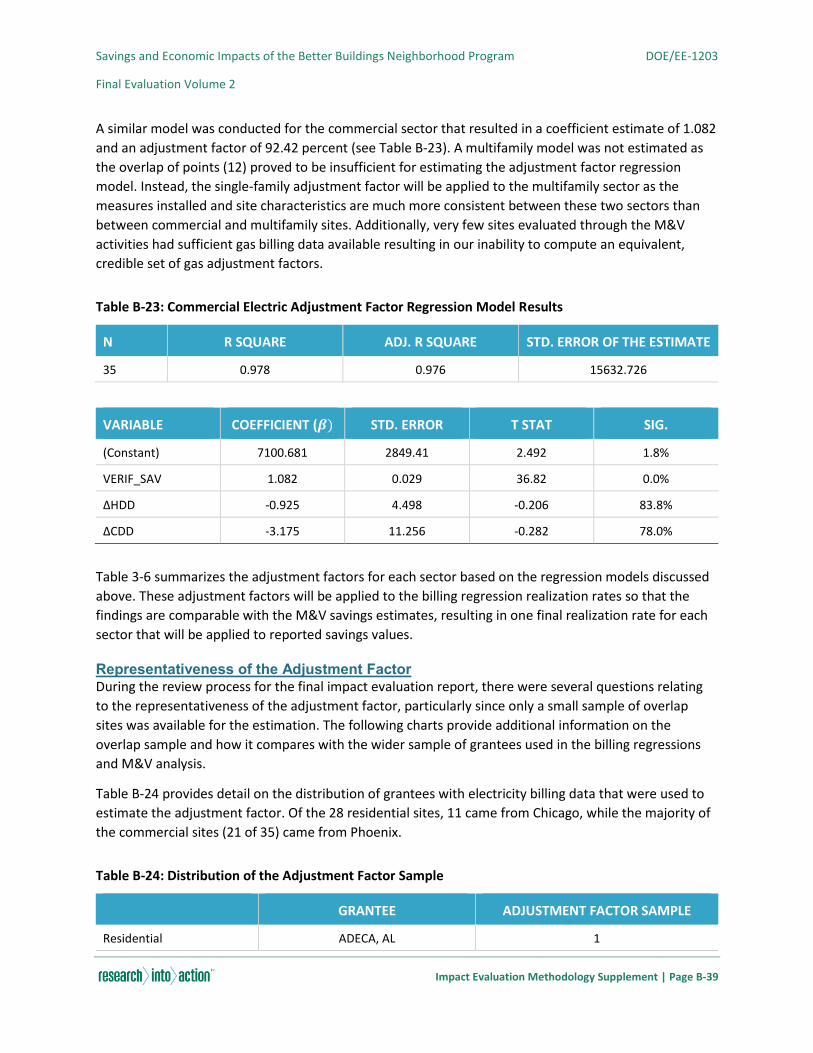
Savings and Economic Impacts of the Better Buildings Neighborhood Program DOE/EE-1203
Final Evaluation Volume 2
Impact Evaluation Methodology Supplement | Page B-39
A similar model was conducted for the commercial sector that resulted in a coefficient estimate of 1.082
and an adjustment factor of 92.42 percent (see Table B-23). A multifamily model was not estimated as
the overlap of points (12) proved to be insufficient for estimating the adjustment factor regression
model. Instead, the single-family adjustment factor will be applied to the multifamily sector as the
measures installed and site characteristics are much more consistent between these two sectors than
between commercial and multifamily sites. Additionally, very few sites evaluated through the M&V
activities had sufficient gas billing data available resulting in our inability to compute an equivalent,
credible set of gas adjustment factors.
Table B-23: Commercial Electric Adjustment Factor Regression Model Results
N R SQUARE ADJ. R SQUARE STD. ERROR OF THE ESTIMATE
35 0.978 0.976 15632.726
VARIABLE COEFFICIENT (𝜷) STD. ERROR T STAT SIG.
(Constant) 7100.681 2849.41 2.492 1.8%
VERIF_SAV 1.082 0.029 36.82 0.0%
ΔHDD -0.925 4.498 -0.206 83.8%
ΔCDD -3.175 11.256 -0.282 78.0%
Table 3-6 summarizes the adjustment factors for each sector based on the regression models discussed
above. These adjustment factors will be applied to the billing regression realization rates so that the
findings are comparable with the M&V savings estimates, resulting in one final realization rate for each
sector that will be applied to reported savings values.
Representativeness of the Adjustment Factor During the review process for the final impact evaluation report, there were several questions relating
to the representativeness of the adjustment factor, particularly since only a small sample of overlap
sites was available for the estimation. The following charts provide additional information on the
overlap sample and how it compares with the wider sample of grantees used in the billing regressions
and M&V analysis.
Table B-24 provides detail on the distribution of grantees with electricity billing data that were used to
estimate the adjustment factor. Of the 28 residential sites, 11 came from Chicago, while the majority of
the commercial sites (21 of 35) came from Phoenix.
Table B-24: Distribution of the Adjustment Factor Sample
GRANTEE ADJUSTMENT FACTOR SAMPLE
Residential ADECA, AL 1
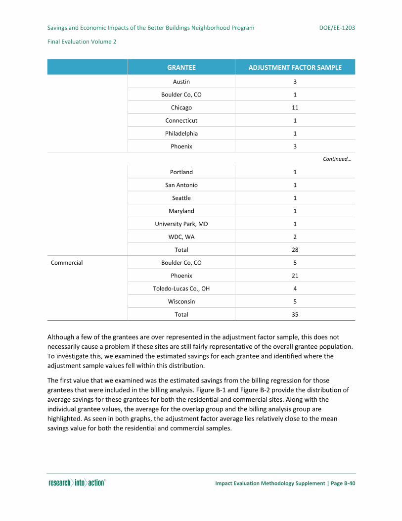
Savings and Economic Impacts of the Better Buildings Neighborhood Program DOE/EE-1203
Final Evaluation Volume 2
Impact Evaluation Methodology Supplement | Page B-40
GRANTEE ADJUSTMENT FACTOR SAMPLE
Austin 3
Boulder Co, CO 1
Chicago 11
Connecticut 1
Philadelphia 1
Phoenix 3
Continued…
Portland 1
San Antonio 1
Seattle 1
Maryland 1
University Park, MD 1
WDC, WA 2
Total 28
Commercial Boulder Co, CO 5
Phoenix 21
Toledo-Lucas Co., OH 4
Wisconsin 5
Total 35
Although a few of the grantees are over represented in the adjustment factor sample, this does not
necessarily cause a problem if these sites are still fairly representative of the overall grantee population.
To investigate this, we examined the estimated savings for each grantee and identified where the
adjustment sample values fell within this distribution.
The first value that we examined was the estimated savings from the billing regression for those
grantees that were included in the billing analysis. Figure B-1 and Figure B-2 provide the distribution of
average savings for these grantees for both the residential and commercial sites. Along with the
individual grantee values, the average for the overlap group and the billing analysis group are
highlighted. As seen in both graphs, the adjustment factor average lies relatively close to the mean
savings value for both the residential and commercial samples.
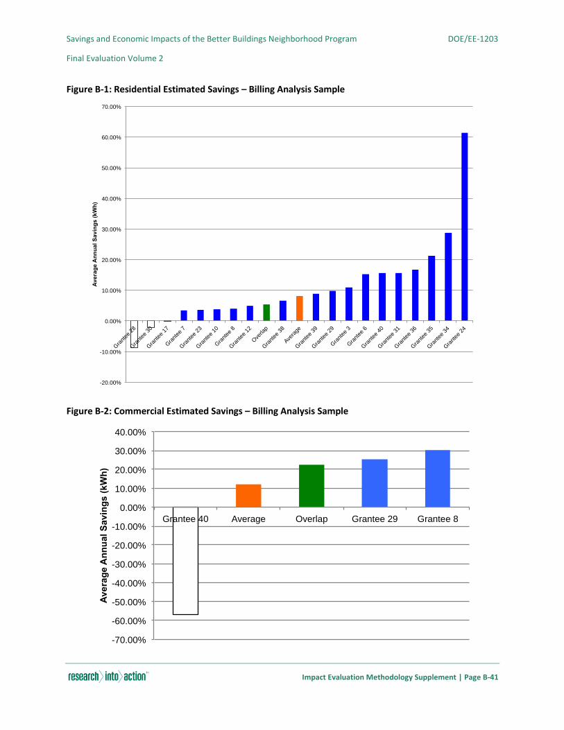
Savings and Economic Impacts of the Better Buildings Neighborhood Program DOE/EE-1203
Final Evaluation Volume 2
Impact Evaluation Methodology Supplement | Page B-41
Figure B-1: Residential Estimated Savings – Billing Analysis Sample
Figure B-2: Commercial Estimated Savings – Billing Analysis Sample
-20.00%
-10.00%
0.00%
10.00%
20.00%
30.00%
40.00%
50.00%
60.00%
70.00%
Gra
ntee
28
Gra
ntee
30
Gra
ntee
17
Gra
ntee
7
Gra
ntee
23
Gra
ntee
10
Gra
ntee
8
Gra
ntee
12
Ove
rlap
Gra
ntee
38
Avera
ge
Gra
ntee
39
Gra
ntee
29
Gra
ntee
3
Gra
ntee
6
Gra
ntee
40
Gra
ntee
31
Gra
ntee
36
Gra
ntee
35
Gra
ntee
34
Gra
ntee
24
Av
era
ge
An
nu
al
Sa
vin
gs
(k
Wh
)
-70.00%
-60.00%
-50.00%
-40.00%
-30.00%
-20.00%
-10.00%
0.00%
10.00%
20.00%
30.00%
40.00%
Grantee 40 Average Overlap Grantee 29 Grantee 8
Ave
rag
e A
nn
ual S
avin
gs
(k
Wh
)
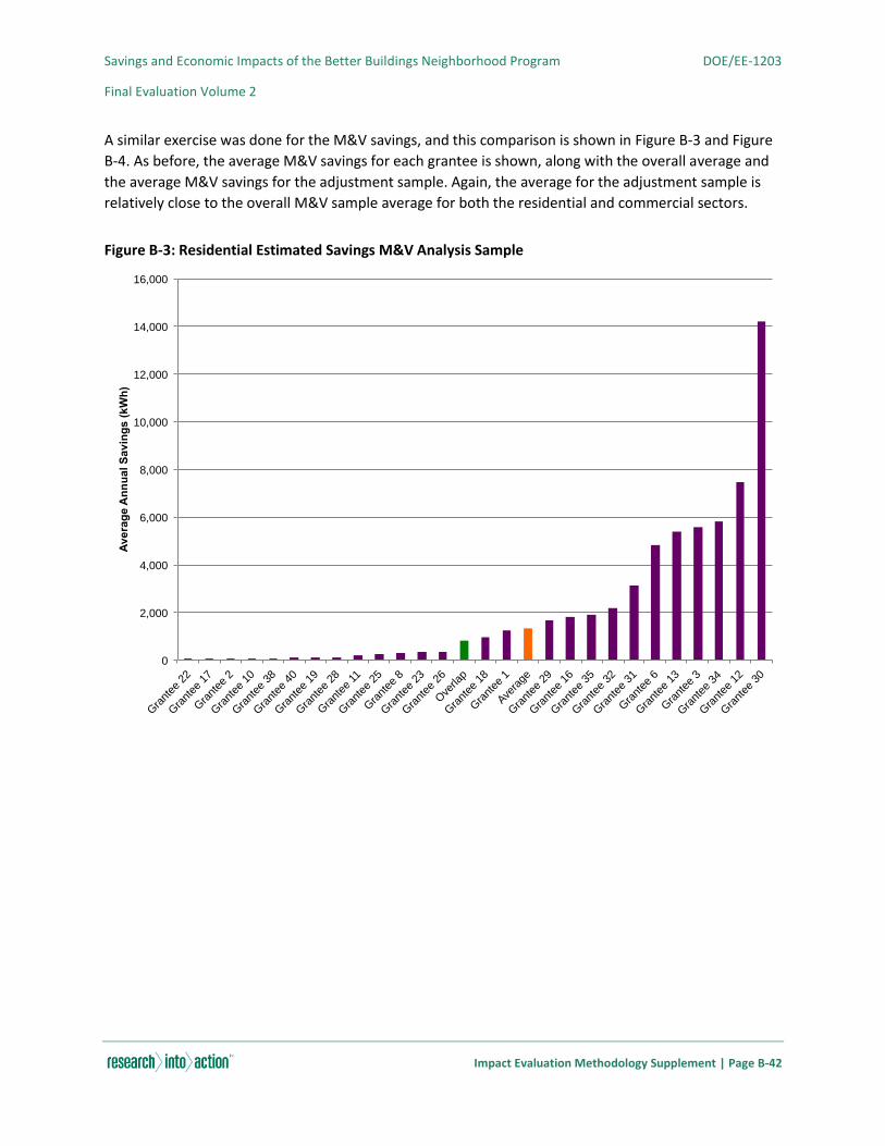
Savings and Economic Impacts of the Better Buildings Neighborhood Program DOE/EE-1203
Final Evaluation Volume 2
Impact Evaluation Methodology Supplement | Page B-42
A similar exercise was done for the M&V savings, and this comparison is shown in Figure B-3 and Figure
B-4. As before, the average M&V savings for each grantee is shown, along with the overall average and
the average M&V savings for the adjustment sample. Again, the average for the adjustment sample is
relatively close to the overall M&V sample average for both the residential and commercial sectors.
Figure B-3: Residential Estimated Savings M&V Analysis Sample
0
2,000
4,000
6,000
8,000
10,000
12,000
14,000
16,000
Gra
ntee
22
Gra
ntee
17
Gra
ntee
2
Gra
ntee
10
Gra
ntee
38
Gra
ntee
40
Gra
ntee
19
Gra
ntee
28
Gra
ntee
11
Gra
ntee
25
Gra
ntee
8
Gra
ntee
23
Gra
ntee
26
Ove
rlap
Gra
ntee
18
Gra
ntee
1
Avera
ge
Gra
ntee
29
Gra
ntee
16
Gra
ntee
35
Gra
ntee
32
Gra
ntee
31
Gra
ntee
6
Gra
ntee
13
Gra
ntee
3
Gra
ntee
34
Gra
ntee
12
Gra
ntee
30
Ave
rag
e A
nn
ual
Sav
ing
s (
kW
h)
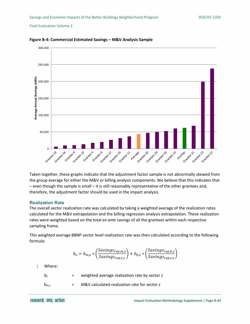
Savings and Economic Impacts of the Better Buildings Neighborhood Program DOE/EE-1203
Final Evaluation Volume 2
Impact Evaluation Methodology Supplement | Page B-43
Figure B-4: Commercial Estimated Savings – M&V Analysis Sample
Taken together, these graphs indicate that the adjustment factor sample is not abnormally skewed from
the group average for either the M&V or billing analysis components. We believe that this indicates that
– even though the sample is small – it is still reasonably representative of the other grantees and,
therefore, the adjustment factor should be used in the impact analysis.
Realization Rate The overall sector realization rate was calculated by taking a weighted average of the realization rates
calculated for the M&V extrapolation and the billing regression analysis extrapolation. These realization
rates were weighted based on the total ex ante savings of all the grantees within each respective
sampling frame.
This weighted average BBNP sector level realization rate was then calculated according to the following
formula:
𝑏𝑧 = 𝑏𝑚,𝑧 ∗ (𝑆𝑎𝑣𝑖𝑛𝑔𝑠𝑟𝑒𝑝,𝑚,𝑧
𝑆𝑎𝑣𝑖𝑛𝑔𝑠𝑟𝑒𝑝,𝑡,𝑧) + 𝑏𝑏,𝑧 ∗ (
𝑆𝑎𝑣𝑖𝑛𝑔𝑠𝑟𝑒𝑝,𝑏,𝑧
𝑆𝑎𝑣𝑖𝑛𝑔𝑠𝑟𝑒𝑝,𝑡,𝑧)
Where:
bz = weighted average realization rate by sector z
bm,z = M&V calculated realization rate for sector z
0
50,000
100,000
150,000
200,000
250,000
300,000
Gra
ntee
18
Gra
ntee
34
Gra
ntee
9
Gra
ntee
19
Gra
ntee
5
Gra
ntee
8
Gra
ntee
37
Gra
ntee
25
Gra
ntee
11
Avera
ge
Gra
ntee
40
Gra
ntee
29
Gra
ntee
30
Gra
ntee
10
Ove
rlap
Gra
ntee
31
Gra
ntee
23
Gra
ntee
22
Avera
ge
An
nu
al S
avin
gs (
kW
h)

Savings and Economic Impacts of the Better Buildings Neighborhood Program DOE/EE-1203
Final Evaluation Volume 2
Impact Evaluation Methodology Supplement | Page B-44
bb,z = billing regression analysis calculated realization rate for sector z
z = residential or commercial
Savingsrep,m,z = reported savings for all grantees within M&V sample frame for sector z
Savingsrep,b,z = reported savings for all grantees within Billing regression analysis sample
frame for sector z
Savingsrep,t,z = total reported savings for all grantees in sector z
Once the weighted average realization rate was determined, this value was applied to the overall
reported savings to determine a gross verified savings by sector.
𝑆𝑎𝑣𝑖𝑛𝑔𝑠𝑔𝑟𝑜𝑠𝑠 𝑣𝑒𝑟,𝑧 = 𝑆𝑎𝑣𝑖𝑛𝑔𝑠𝑟𝑒𝑝,𝑧 ∗ 𝑏𝑧
Where:
bz = weighted average realization rate by sector z
z = residential or commercial
Savingsrep,z = total reported savings for sector z
Savingsgross ver,z = total gross verified savings for sector z
The total gross verified savings for BBNP was calculated as the sum of the sector gross verified savings.
Thus, the overall gross verified savings for BBNP is calculated as:
𝑆𝑎𝑣𝑖𝑛𝑔𝑠𝑔𝑟𝑜𝑠𝑠 𝑣𝑒𝑟,𝐵𝐵𝑁𝑃 = ∑ 𝑆𝑎𝑣𝑖𝑛𝑔𝑠𝑔𝑟𝑜𝑠𝑠 𝑣𝑒𝑟,𝑧
𝑧
Where:
Savingsgross ver,BBNP = total gross verified savings of BBNP
Savingsgross ver,z = total gross verified savings for sector z
Net verified savings for each sector were determined by applying the NTG ratio found in the
influence/spillover analysis to the sector level gross verified savings from the verification sample only:
𝑆𝑎𝑣𝑖𝑛𝑔𝑠𝑛𝑒𝑡 𝑣𝑒𝑟,𝑧 = 𝑆𝑎𝑣𝑖𝑛𝑔𝑠𝑔𝑟𝑜𝑠𝑠 𝑣𝑒𝑟,𝑧 ∗ 𝑁𝑇𝐺𝑧
Where:
𝑁𝑇𝐺𝑧 = net-to-gross ratio for sector z = residential or commercial
Savingsgross ver,z = total gross verified savings for sector z
Savingsnet ver,z = total net verified savings for sector z
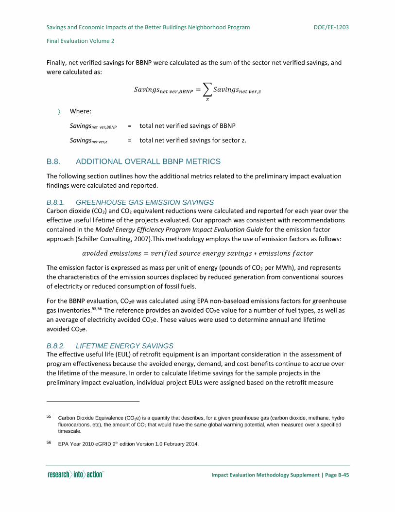
Savings and Economic Impacts of the Better Buildings Neighborhood Program DOE/EE-1203
Final Evaluation Volume 2
Impact Evaluation Methodology Supplement | Page B-45
Finally, net verified savings for BBNP were calculated as the sum of the sector net verified savings, and
were calculated as:
𝑆𝑎𝑣𝑖𝑛𝑔𝑠𝑛𝑒𝑡 𝑣𝑒𝑟,𝐵𝐵𝑁𝑃 = ∑ 𝑆𝑎𝑣𝑖𝑛𝑔𝑠𝑛𝑒𝑡 𝑣𝑒𝑟,𝑧
𝑧
Where:
Savingsnet ver,BBNP = total net verified savings of BBNP
Savingsnet ver,z = total net verified savings for sector z.
B.8. ADDITIONAL OVERALL BBNP METRICS
The following section outlines how the additional metrics related to the preliminary impact evaluation
findings were calculated and reported.
B.8.1. GREENHOUSE GAS EMISSION SAVINGS Carbon dioxide (CO2) and CO2 equivalent reductions were calculated and reported for each year over the
effective useful lifetime of the projects evaluated. Our approach was consistent with recommendations
contained in the Model Energy Efficiency Program Impact Evaluation Guide for the emission factor
approach (Schiller Consulting, 2007).This methodology employs the use of emission factors as follows:
𝑎𝑣𝑜𝑖𝑑𝑒𝑑 𝑒𝑚𝑖𝑠𝑠𝑖𝑜𝑛𝑠 = 𝑣𝑒𝑟𝑖𝑓𝑖𝑒𝑑 𝑠𝑜𝑢𝑟𝑐𝑒 𝑒𝑛𝑒𝑟𝑔𝑦 𝑠𝑎𝑣𝑖𝑛𝑔𝑠 ∗ 𝑒𝑚𝑖𝑠𝑠𝑖𝑜𝑛𝑠 𝑓𝑎𝑐𝑡𝑜𝑟
The emission factor is expressed as mass per unit of energy (pounds of CO2 per MWh), and represents
the characteristics of the emission sources displaced by reduced generation from conventional sources
of electricity or reduced consumption of fossil fuels.
For the BBNP evaluation, CO2e was calculated using EPA non-baseload emissions factors for greenhouse
gas inventories.55,56 The reference provides an avoided CO2e value for a number of fuel types, as well as
an average of electricity avoided CO2e. These values were used to determine annual and lifetime
avoided CO2e.
B.8.2. LIFETIME ENERGY SAVINGS The effective useful life (EUL) of retrofit equipment is an important consideration in the assessment of
program effectiveness because the avoided energy, demand, and cost benefits continue to accrue over
the lifetime of the measure. In order to calculate lifetime savings for the sample projects in the
preliminary impact evaluation, individual project EULs were assigned based on the retrofit measure
55 Carbon Dioxide Equivalence (CO2e) is a quantity that describes, for a given greenhouse gas (carbon dioxide, methane, hydro
fluorocarbons, etc), the amount of CO2 that would have the same global warming potential, when measured over a specified
timescale.
56 EPA Year 2010 eGRID 9th edition Version 1.0 February 2014.
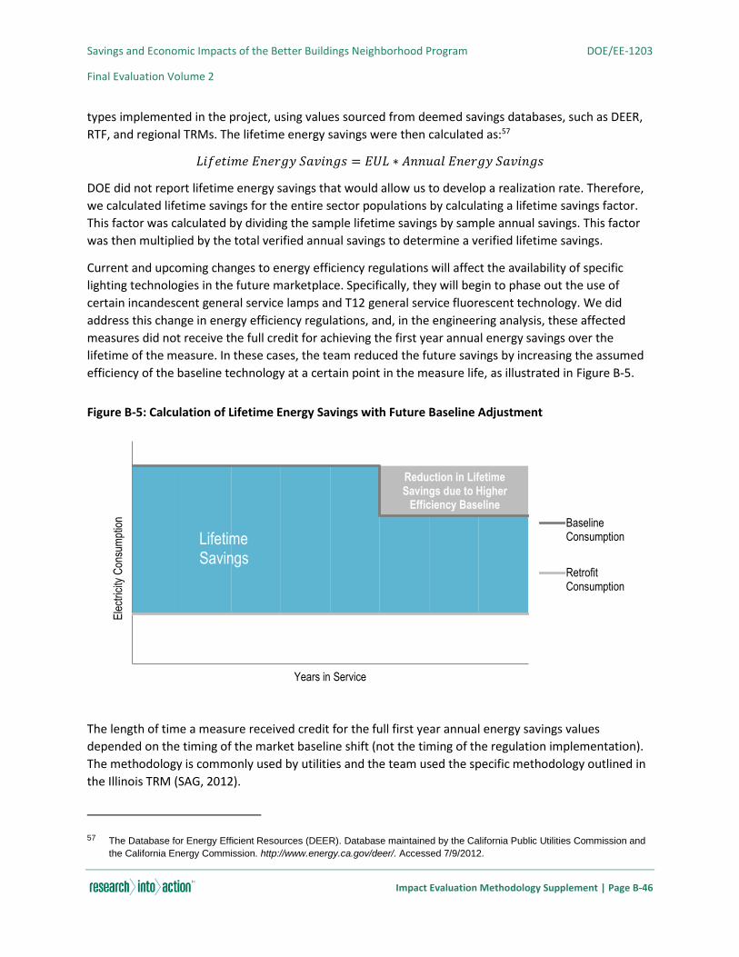
Savings and Economic Impacts of the Better Buildings Neighborhood Program DOE/EE-1203
Final Evaluation Volume 2
Impact Evaluation Methodology Supplement | Page B-46
types implemented in the project, using values sourced from deemed savings databases, such as DEER,
RTF, and regional TRMs. The lifetime energy savings were then calculated as:57
𝐿𝑖𝑓𝑒𝑡𝑖𝑚𝑒 𝐸𝑛𝑒𝑟𝑔𝑦 𝑆𝑎𝑣𝑖𝑛𝑔𝑠 = 𝐸𝑈𝐿 ∗ 𝐴𝑛𝑛𝑢𝑎𝑙 𝐸𝑛𝑒𝑟𝑔𝑦 𝑆𝑎𝑣𝑖𝑛𝑔𝑠
DOE did not report lifetime energy savings that would allow us to develop a realization rate. Therefore,
we calculated lifetime savings for the entire sector populations by calculating a lifetime savings factor.
This factor was calculated by dividing the sample lifetime savings by sample annual savings. This factor
was then multiplied by the total verified annual savings to determine a verified lifetime savings.
Current and upcoming changes to energy efficiency regulations will affect the availability of specific
lighting technologies in the future marketplace. Specifically, they will begin to phase out the use of
certain incandescent general service lamps and T12 general service fluorescent technology. We did
address this change in energy efficiency regulations, and, in the engineering analysis, these affected
measures did not receive the full credit for achieving the first year annual energy savings over the
lifetime of the measure. In these cases, the team reduced the future savings by increasing the assumed
efficiency of the baseline technology at a certain point in the measure life, as illustrated in Figure B-5.
Figure B-5: Calculation of Lifetime Energy Savings with Future Baseline Adjustment
The length of time a measure received credit for the full first year annual energy savings values
depended on the timing of the market baseline shift (not the timing of the regulation implementation).
The methodology is commonly used by utilities and the team used the specific methodology outlined in
the Illinois TRM (SAG, 2012).
57 The Database for Energy Efficient Resources (DEER). Database maintained by the California Public Utilities Commission and
the California Energy Commission. http://www.energy.ca.gov/deer/. Accessed 7/9/2012.
Ele
ctric
ity C
onsu
mpt
ion
Years in Service
BaselineConsumption
RetrofitConsumption
Lifetime Savings
Reduction in Lifetime Savings due to Higher
Efficiency Baseline
Savings and Economic Impacts of the Better Buildings Neighborhood Program DOE/EE-1203
Final Evaluation Volume 2
Impact Evaluation Methodology Supplement | Page B-47
B.9. ECONOMIC IMPACT ANALYSIS METHODS
A separate portion of the impact evaluation is to estimate BBNP’s economic impacts.
B.9.1. ANALYSIS METHODS The goal of an economic impact analysis of an energy efficiency program is twofold. The analysis should
inform interested stakeholders and the public, as well as provide useful, action-oriented information to
policymakers and program managers. To that end, the economic impact analysis should: 1) rely on
program-specific data whenever possible; 2) be based on a reliable and transparent modeling
framework; 3) fully document the modeling approach, the assumptions and limitations of that
approach; and 4) report the full range of economic impact results and produce economic impact metrics
that policy makers can use to improve program performance or affect program outcomes.
In contrast to the energy impact analysis, we utilized the Program Level information contained in the
BBNP Quarterly Summary Reports to analyze the economic impact of the program offerings. These
reports were used rather than the Project Level data as they contained the information needed for this
analysis including program outlays, energy bill savings, and measure spending. As the two primary data
sources slightly differ, discrepancies between the energy impact analysis and the economic analysis may
exist.
Overview
Measuring the economic impacts estimated for BBNP is a complex process, as spending by grantees and
program participants unfold over time for over 40 separate grantee offerings. From this perspective, the
most appropriate analytical framework for estimating the economic impacts is to classify them into
short-term and long-term impacts:
Short-term impacts are associated with changes in business activity as a direct result of changes
in spending (or final demand) by program administrators, program participants, and institutions
that provide funding for energy efficiency programs.
Long-term impacts are associated with the potential changes in relative prices, factor costs, and
the optimal use of resources among program participants, as well as industries and households
linked by competitive, supply-chain, or other factors.
This analysis measures the short-term economic impacts approximated for BBNP. These impacts are
driven by changes (both positive and negative) in final demand, and are measured within a static input-
output modeling framework that relies on data for an economy at a point in time and assumes that
program spending does not affect the evolution of the economy. (This last event is what economists call
a change in the “production possibilities frontier” of the economy.) Energy efficiency programs may
have longer lasting effects, and this is clearly the case for continued post-installation energy savings.
However, long-term, dynamic effects are not measured in this analysis, as it is unlikely that BBNP is
causing significant structural changes in the economy given the relatively small magnitude of energy
savings achieved relative to the overall size of the national economy.

Savings and Economic Impacts of the Better Buildings Neighborhood Program DOE/EE-1203
Final Evaluation Volume 2
Impact Evaluation Methodology Supplement | Page B-48
Input-Output Modeling Framework The economic modeling framework that best measures these short-term economic impacts is called
input-output modeling. Input-output models involve mathematical representations of the economy that
describe how different parts (or sectors) are linked to one another. There are several important points
about input-output models that should be noted:
Input-output models provide a reasonably comprehensive picture of the economic activities
within an economy and can be constructed for almost any study area.
Input-output models use a simple, rectangular accounting framework called double-entry
accounting. This results in a model structure that is well ordered, symmetric, and where, by
definition, inputs must be equal to outputs.
Input-output models are static models in that they measure the flow of inputs and outputs in
an economy at a point in time. With this information and the balanced accounting structure of
an input-output model, an analyst can: 1) describe an economy at one time period; 2) introduce
a change to the economy; and then 3) evaluate the economy after it has accommodated that
change. This type of analysis is called partial equilibrium analysis.
In order to provide a common unit of measure, all transaction flows in an input-output model
are stated in dollars.
The IMPLAN Model
This analysis relies on an economic impact model of the U.S. economy constructed using the IMPLAN
(for IMpact Analysis for PLANning) modeling software.58 IMPLAN has several features that make it
particularly well suited for this analysis:
IMPLAN is widely used and well respected. IMPLAN models are constructed with data
assembled for national income accounting purposes, thereby providing a tool that has a robust
link to widely accepted data development efforts. The United States Department of Agriculture
(USDA) recognized the IMPLAN modeling framework as “one of the most credible regional
impact models used for regional economic impact analysis” and, following a review by experts
from seven USDA agencies, selected IMPLAN as its analysis framework for monitoring job
creation associated with the ARRA.59
The IMPLAN model’s detailed descriptive capabilities provide a full characterization of the U.S.
economy, in, this case, 2011. The IMPLAN model has a wide range of economic data for 440
different industry sectors, as well as for households and government institutions.
58 IMPLAN (for IMpact Analysis for PLANning) was originally developed by the Forest Service of the U.S. Department of
Agriculture in cooperation with the Federal Emergency Management Agency and the Bureau of Land Management of the U.S.
Department of the Interior in 1993, and is currently licensed and distributed by the IMPLAN Group LLC.
59 See excerpts from an April 9, 2009 letter to MIG, Inc., from John Kort, Acting Administrator of the USDA Economic Research
Service, on behalf of Secretary Vilsack, at www.implan.com.

Savings and Economic Impacts of the Better Buildings Neighborhood Program DOE/EE-1203
Final Evaluation Volume 2
Impact Evaluation Methodology Supplement | Page B-49
The logical input-output modeling framework and detailed economic data within the IMPLAN
model provide the structure necessary to adjust economic relationships or to build custom
production functions for spending and activities that are linked back to BBNP. This detailed
and flexible modeling system permits the most accurate mapping of BBNP program and
participant spending, and energy savings, to industry and household sectors in the IMPLAN
model.
Terminology and Impact Metrics
Input-output analysis employs specific terminology to identify the different types of economic impacts.
BBNP affects the economy directly, through the purchases of goods and services. Under our program-
centric approach, these direct impacts include jobs (person-years of employment)60 and income for
grantee staff that administer and manage energy efficiency programs, contractors who provide audit
and retrofit services, and energy efficiency equipment manufacturers. Direct impacts also include
changes in spending or output resulting from the energy savings for participating households and
businesses.
These direct changes in economic activity will, in turn, indirectly generate purchases of intermediate
goods and services from other, related sectors of the economy. Because these indirect purchases
represent interactions among businesses, they are often referred to as “supply-chain” impacts.
In addition, the direct and indirect increases in employment and income enhance overall economy
purchasing power, thereby inducing further consumption- and investment- driven stimulus. These
induced effects are often referred to as “consumption-driven” impacts. In this report, the indirect and
induced impacts are grouped together and reported as “secondary” impacts.
The IMPLAN model reports the following impact measures:
Output is the value of production for a specified period of time. Output is the broadest measure
of economic activity, and includes intermediate goods and services and the components of value
added (personal income, other income, and indirect business taxes). As such, output and
personal income should not be added together.
Personal income is the sum of wages and business income.
Wages includes workers’ wages and salaries, as well as other benefits such as health and life
insurance, retirement payments, and noncash compensation.
Business income also is called proprietary income (or small business income) and represents
the payments received by small-business owners or self-employed workers. Business
60 The term “person-year of employment” is often used when measuring jobs to emphasize the transitory nature of program-
related employment. In the case of these BBNP programs, the initial employment will last as long as program funding is
available to encourage the installation of energy efficient equipment. As discussed earlier in the report, longer term
employment gains also occur due to energy bill savings enjoyed by customers over the life of the equipment. For reporting
purposes, all IMPLAN job estimates in this report have been converted to full-time equivalents, which represent a very specific
person-year of employment (that is, a worker employed at least 2,080 hours in a standard year).

Savings and Economic Impacts of the Better Buildings Neighborhood Program DOE/EE-1203
Final Evaluation Volume 2
Impact Evaluation Methodology Supplement | Page B-50
income would include, for example, income received by private business owners including
doctors, accountants, lawyers, and others.
Job impacts include both full- and part-time employment. These job impacts are measured in
person-years of employment, and reported as full-time equivalent (FTE).61
All of the economic impacts in this analysis are transitory and depend on program spending by BBNP
grantees, as well as spending and energy savings for program participants. As discussed previously,
economic impacts are estimated for program outcomes over the Q1 2010 through Q3 2013 time period.
Because this twelve-quarter time period includes partial years in 2010 and 2013, the economic impact
modeling was conducted on a quarterly basis. Economic impact modeling on a quarterly basis presents
certain complications, and it is important to understand the modeling issues associated with such
analyses and how they affect the reporting of modeling results.
There are two main issues with quarterly analyses. First, the economic relationships in the IMPLAN
model are based on annual data (for example, average annual output or income per worker). Second,
the secondary spending effects are assumed to take place over a year even though the timing of the
direct spending effects is known. Simply put, it takes time for the supply-chain and consumption-driven
spending effects to ripple through the economy, with most analyses assuming this duration to be one
year.
In most cases, summing quarterly spending across years can address these issues. In this analysis, partial
years of activity in 2010 and 2013 prevent this outcome. Instead, the direct effects are assumed (or,
more precisely, known) to occur in each quarter, with the direct job effects multiplied by four (the
number of quarters in a year) while the direct monetary effects are not adjusted. For example, $1
million in spending for a labor-only service, where the average annual wage is $100,000, will generate
10 jobs over the course of a year (that is, the equivalent of ten positions each lasting one year or ten
person-years of employment). Instead, if this $1 million in spending occurred in one quarter, it would
support 40 jobs in that quarter (that is, person-quarter-years of employment). It is clear from this
example that the average earnings for this quarter-year of work are $25,000, consistent with an average
annual wage of $100,000 for a single person working fulltime. Perhaps more importantly, the 40 “jobs”
in the quarter are equivalent to 10 person-years of employment, which is consistent with the initial
example of 10 direct jobs if this spending occurred over the course of an entire year.
Gross and Net Impacts
Citing the economic impacts that occur as a result of an efficiency program provides an upper bound
estimate of impacts. This upper bound estimate is often referred to as a measure of the gross economic
impacts. Gross economic impacts offer a perspective on the magnitude of overall impacts that can be
61 The IMPLAN modeling software measures jobs as the annual average of monthly jobs in each industry (this is the same
definition used by Quarterly Census of Employment and Wages [QCEW], U.S. Bureau of Labor Statistics [BLS], and U.S.
Bureau of Economic Analysis [BEA] nationally). Thus, one job is equivalent to one person being employed for the duration of
one year, two people being employed for half a year each, three people being employed for a third of a year each, etc.
Furthermore, IMPLAN jobs include full-time, part-time, and temporary positions. For reporting purposes, all IMPLAN job
estimates in this report have been converted to full-time equivalents (2,080 hours in a standard year).

Savings and Economic Impacts of the Better Buildings Neighborhood Program DOE/EE-1203
Final Evaluation Volume 2
Impact Evaluation Methodology Supplement | Page B-51
traced back to the program; however, they do not necessarily reflect or measure the creation of new
jobs or income.
An analysis of the net economic impacts requires that only economic stimuli that are new or additive to
the economy be counted. To address this, the impact analysis first defines a Base Case scenario that
describes what would have happened in the absence of the program. This base case scenario is typically
implemented by posting a counterfactual argument that only counts economic activity that “but for” the
program would not have occurred. The distinction between gross and net impacts for BBNP is important
because federal funding used to support grantee energy efficiency programs will divert spending from
other federal government programs. An additional alternative counterfactual also is explored and
outlined in more detail in the next section of the report.
For energy efficiency programs, the gross economic impacts reflect the economic impacts without
adjustments for impacts that might have occurred from spending in the base case scenario. Gross
impacts include:
Program outlays as BBNP grantees incur administrative costs, and purchase labor and materials
to carry out their energy efficiency programs. (There are three major categories of program
outlays, and these are discussed in detail in the next section of the report.)
Measure spending represents spending on efficiency upgrades. Measure spending is allocated
to equipment and labor, mapped to North American Industry Classification System (NAICS)
codes, and then mapped to sectors in the economic impact model.
Reductions in energy consumption and the associated increase in household disposable income
and lower operating costs for businesses.62
For residential program participants, lower energy costs will increase household
disposable income. These estimated residential energy bill savings are fed into a modified
household consumption function (household spending on goods and services less
expenditures on energy) to estimate how this additional spending affects the economy.
For businesses, energy savings lowers production costs, which, in the short run, leads to
changes in output. To estimate the economic impacts associated with these lower energy
costs, the project team implemented a 1-for-1 dollar change (that is, a $1 decrease in energy
costs was assumed to be equivalent to an increase in production by $1).63
62 Both a realization rate adjustment and a net-to-gross adjusted will be applied to the energy bill savings in the final evaluation
report. For the preliminary evaluation, the gross and net energy impact analysis was not completed in time for either of these
adjustments to be incorporated into the economic impact analysis. The net-to-gross adjustment also will be applied to measure
spending in the economic analysis conducted for the final evaluation report.
63 An economic impact analysis of a proposed cap-and-trade emissions reduction strategy conducted by ECONorthwest
corroborates this method. This analysis found that the elasticity of production relative to energy costs was very close to -1.0 for
many sectors of the economy. More details are available at:
http://www.ecy.wa.gov/climatechange/docs/20100707_wci_econanalysis.pdf
Savings and Economic Impacts of the Better Buildings Neighborhood Program DOE/EE-1203
Final Evaluation Volume 2
Impact Evaluation Methodology Supplement | Page B-52
Reductions in utility revenues as households and businesses consume less electricity. To be
balanced in our analysis, these revenue decreases are included in the analysis. To be consistent
with reductions in energy consumption, these revenue decreases are included in post-
installation quarters between Q1 2010 and Q3 2013. They are not, however, included in annual
energy savings impacts beyond this twelve-quarter period.
The net economic impacts estimated for BBNP include adjustments to reflect the economic activity that
occurs in the base case scenario. That is, net impacts are those impacts over and above what would
have occurred in the base case scenario. The net economic impacts estimated for BBNP are based on:
Gross program impacts (discussed above).
Less foregone federal spending on nondefense programs as a result of the federal funding that
is allocated to BBNP grantees.
B.9.2. MODEL INPUT DATA The economic analysis relies on data for BBNP spending and activities between Q1 2010 and Q3 2013, as
gathered from DOE Quarterly Summary Reports and, where necessary, detailed quarterly spreadsheets
completed by program grantees. There are limitations to these data as they relate to the economic
impact analysis. That is, these data were gathered to monitor program performance and potential
market transformation effects. In some instances, detailed spending data necessary for economic
impact modeling were not explicitly reported. Moreover, these data were gathered from 41 BBNP
grantees, each implementing their own energy efficiency program(s). Thus, there was a degree of
inconsistency in reporting across grantees.
BBNP tracks grantee spending for three major outlay categories: Marketing and Outreach (M&O), Labor
and Materials (L&M), and Other. BBNP also tracks certain data for three major activity categories: audits
(assessments), energy upgrades (retrofits), and loans. These outlay and activity categories are discussed
in more detail below, as they relate to the economic impact analysis. They have been reorganized
somewhat to facilitate the economic impact modeling process.
Outlays
BBNP outlays (or program expenditures) are reported, by grantee and quarter, for three major outlay
categories in the Quarterly Summary Reports. These outlays are summarized in Table B-25. Between Q1
2010 and Q3 2013, total program outlays by BBNP grantees amounted to approximately $445.2 million
(87.6% of total funds granted).
Table B-25: BBNP Outlays by Major Outlay Category
QUARTER / YEAR MARKETING &
OUTREACH
(M&O)
LABOR &
MATERIALS
(L&M)
OTHER TOTAL OUTLAYS
Q1 2010 $2,112,592 $2,132,578 $12,056,392 $16,301,563
Q1 2011 $4,326,945 $1,543,171 $12,202,950 $18,073,066
Savings and Economic Impacts of the Better Buildings Neighborhood Program DOE/EE-1203
Final Evaluation Volume 2
Impact Evaluation Methodology Supplement | Page B-53
QUARTER / YEAR MARKETING &
OUTREACH
(M&O)
LABOR &
MATERIALS
(L&M)
OTHER TOTAL OUTLAYS
Q2 2011 $6,425,745 $10,899,299 $26,142,372 $43,467,417
Q3 2011 $6,738,810 $6,860,799 $26,789,014 $40,388,623
Q4 2011 $6,741,127 $5,964,228 $32,057,431 $44,762,785
Q1 2012 $12,942,750 $5,756,861 $23,798,764 $42,498,375
Continued…
Q2 2012 $6,355,288 $9,803,836 $25,257,991 $41,417,115
Q3 2012 $5,445,143 $14,064,872 $22,416,247 $41,926,261
Q4 2012 $5,394,885 $14,996,178 $25,353,475 $45,744,538
Q1 2013 $3,713,080 $12,411,082 $17,055,328 $33,179,490
Q2 2013 $5,747,231 $15,384,053 $20,366,429 $41,497,713
Q3 2013 $5,271,870 $16,870,443 $13,823,158 $35,965,471
Total All Quarters $71,215,466 $116,687,400 $257,319,550 $445,222,416
Source: BBNP Quarterly Summary Reports.
The data and modeling assumptions for each major outlay category are as follows.
Marketing and Outreach (M&O) outlays totaled $71.2 million between Q1 2010 and Q3 2013.
This represents 16% of total outlays over the twelve quarters. M&O outlays consist of “grant
outlays for communications activities designed to identify, reach and motivate potential
program participants to take actions to either learn more (for example, audit or other
informational activity) energy efficiency or initiate an energy efficiency retrofit at the PROGRAM
level.”64 Total M&O outlays are reported by grantee in the Quarterly Summary Reports. Detailed
M&O activities (for example, business organization outreach, online and traditional advertising,
neighborhood meetings, websites, and webinars) also are reported, by grantee, in the Quarterly
Summary Reports. However, there is no correspondence or conformity between detailed
activities and outlays. That is, detailed M&O spending is not reported. As such, this analysis
applies a dollar-value-weighting factor (or roughly an average cost per M&O activity) to the
reported number of activities taking place each quarter to allocate total M&O spending in that
quarter.
64 Quarterly Programmatic tab in the detailed quarterly spreadsheets.
Savings and Economic Impacts of the Better Buildings Neighborhood Program DOE/EE-1203
Final Evaluation Volume 2
Impact Evaluation Methodology Supplement | Page B-54
Labor and Materials (L&M) outlays totaled $116.7 million (or 26.2% of total outlays) over the
Q1 2010 through Q3 2013 period. According to BBNP reporting instructions, L&M outlays are
“Outlays incurred as part of an audit or retrofit directly associated with the installation of more
energy efficient equipment, appliances, or building components (for example, insulation,
windows, etc.) at the PROGRAM level.”65 Accordingly, L&M outlays are not explicitly included as
inputs into the economic impact model. Rather, they are included as part of audit and efficiency
upgrade (retrofits) activities as follows:
Audit activity is tracked by number of residential and commercial audits completed, by
grantee and quarter, in the Quarterly Summary Reports. Between Q1 2010 and Q3 2013,
BBNP grantees accomplished 225,065 residential audits and 7,635 commercial audits.
Spending on audits, however, is not explicitly reported and, as discussed previously, audit
spending is assumed to be a component of L&M outlays. Using data compiled from the
detailed quarterly spreadsheets submitted by BBNP grantees, audit spending was estimated
by calculating an average audit cost for residential ($264 per audit) and commercial ($772
per audit) audits between Q1 2010 and Q3 2013 and applying those average costs to the
number of residential and commercial audits in each quarter. Audit spending was then
modeled by developing a custom production function for Building Inspection Services
(NAICS 541350) using audit costs and audit hours from the detailed quarterly spreadsheets
to estimate the number of audit jobs (person-years) per million in audit spending.
Energy Upgrades (or retrofits) represent participants’ spending on energy efficiency
upgrades. Although a small, unknown amount of the costs of the energy upgrades is
captured under L&M outlays, most of the costs of energy upgrades are borne by the
participant in the form of out-of-pocket expenses or borrowed funds, or supported through
other federal and nonfederal incentives and funding. As such, the economic impacts
resulting from energy upgrades are, in fact, based on measure spending. Similarly, measure
spending also captures the economic impacts associated with the loans initiated by BBNP
grantees. (Measure spending is discussed in more detail in the next section.)
Other outlays totaled $257.3 million (or 57.8% of total outlays) between Q1 2010 and Q3 2013.
Other outlays consist of “Other program grant outlays at the PROGRAM level not classified as
materials, labor, marketing, or outreach…(they) represent actual grant funds spent on program
delivery and any associated incentives or loans issued during the quarter.”66 Other outlays are
reported in total, by grantee, in the Quarterly Summary Reports. Those reports, however, do not
include additional information to better understand the nature of these other program delivery
costs or to distinguish between program delivery costs and program incentives. This analysis,
therefore, relies on energy efficiency program cost data from the U.S. Energy Information
65 Ibid.
66 Quarterly Programmatic tab in the detailed quarterly spreadsheets.
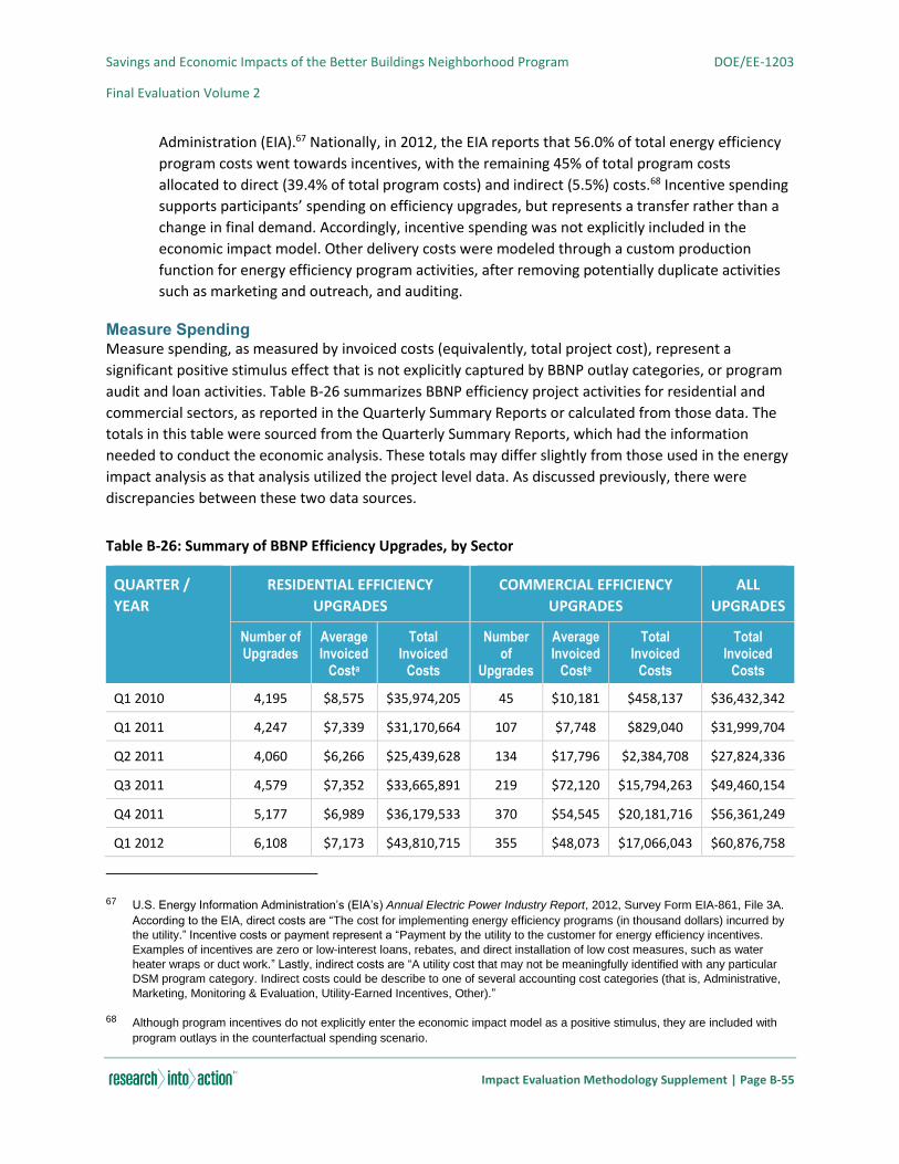
Savings and Economic Impacts of the Better Buildings Neighborhood Program DOE/EE-1203
Final Evaluation Volume 2
Impact Evaluation Methodology Supplement | Page B-55
Administration (EIA).67 Nationally, in 2012, the EIA reports that 56.0% of total energy efficiency
program costs went towards incentives, with the remaining 45% of total program costs
allocated to direct (39.4% of total program costs) and indirect (5.5%) costs.68 Incentive spending
supports participants’ spending on efficiency upgrades, but represents a transfer rather than a
change in final demand. Accordingly, incentive spending was not explicitly included in the
economic impact model. Other delivery costs were modeled through a custom production
function for energy efficiency program activities, after removing potentially duplicate activities
such as marketing and outreach, and auditing.
Measure Spending Measure spending, as measured by invoiced costs (equivalently, total project cost), represent a
significant positive stimulus effect that is not explicitly captured by BBNP outlay categories, or program
audit and loan activities. Table B-26 summarizes BBNP efficiency project activities for residential and
commercial sectors, as reported in the Quarterly Summary Reports or calculated from those data. The
totals in this table were sourced from the Quarterly Summary Reports, which had the information
needed to conduct the economic analysis. These totals may differ slightly from those used in the energy
impact analysis as that analysis utilized the project level data. As discussed previously, there were
discrepancies between these two data sources.
Table B-26: Summary of BBNP Efficiency Upgrades, by Sector
QUARTER /
YEAR
RESIDENTIAL EFFICIENCY
UPGRADES
COMMERCIAL EFFICIENCY
UPGRADES
ALL
UPGRADES
Number of Upgrades
Average Invoiced
Costa
Total Invoiced
Costs
Number of
Upgrades
Average Invoiced
Costa
Total Invoiced
Costs
Total Invoiced
Costs
Q1 2010 4,195 $8,575 $35,974,205 45 $10,181 $458,137 $36,432,342
Q1 2011 4,247 $7,339 $31,170,664 107 $7,748 $829,040 $31,999,704
Q2 2011 4,060 $6,266 $25,439,628 134 $17,796 $2,384,708 $27,824,336
Q3 2011 4,579 $7,352 $33,665,891 219 $72,120 $15,794,263 $49,460,154
Q4 2011 5,177 $6,989 $36,179,533 370 $54,545 $20,181,716 $56,361,249
Q1 2012 6,108 $7,173 $43,810,715 355 $48,073 $17,066,043 $60,876,758
67 U.S. Energy Information Administration’s (EIA’s) Annual Electric Power Industry Report, 2012, Survey Form EIA-861, File 3A.
According to the EIA, direct costs are “The cost for implementing energy efficiency programs (in thousand dollars) incurred by
the utility.” Incentive costs or payment represent a “Payment by the utility to the customer for energy efficiency incentives.
Examples of incentives are zero or low-interest loans, rebates, and direct installation of low cost measures, such as water
heater wraps or duct work.” Lastly, indirect costs are “A utility cost that may not be meaningfully identified with any particular
DSM program category. Indirect costs could be describe to one of several accounting cost categories (that is, Administrative,
Marketing, Monitoring & Evaluation, Utility-Earned Incentives, Other).”
68 Although program incentives do not explicitly enter the economic impact model as a positive stimulus, they are included with
program outlays in the counterfactual spending scenario.
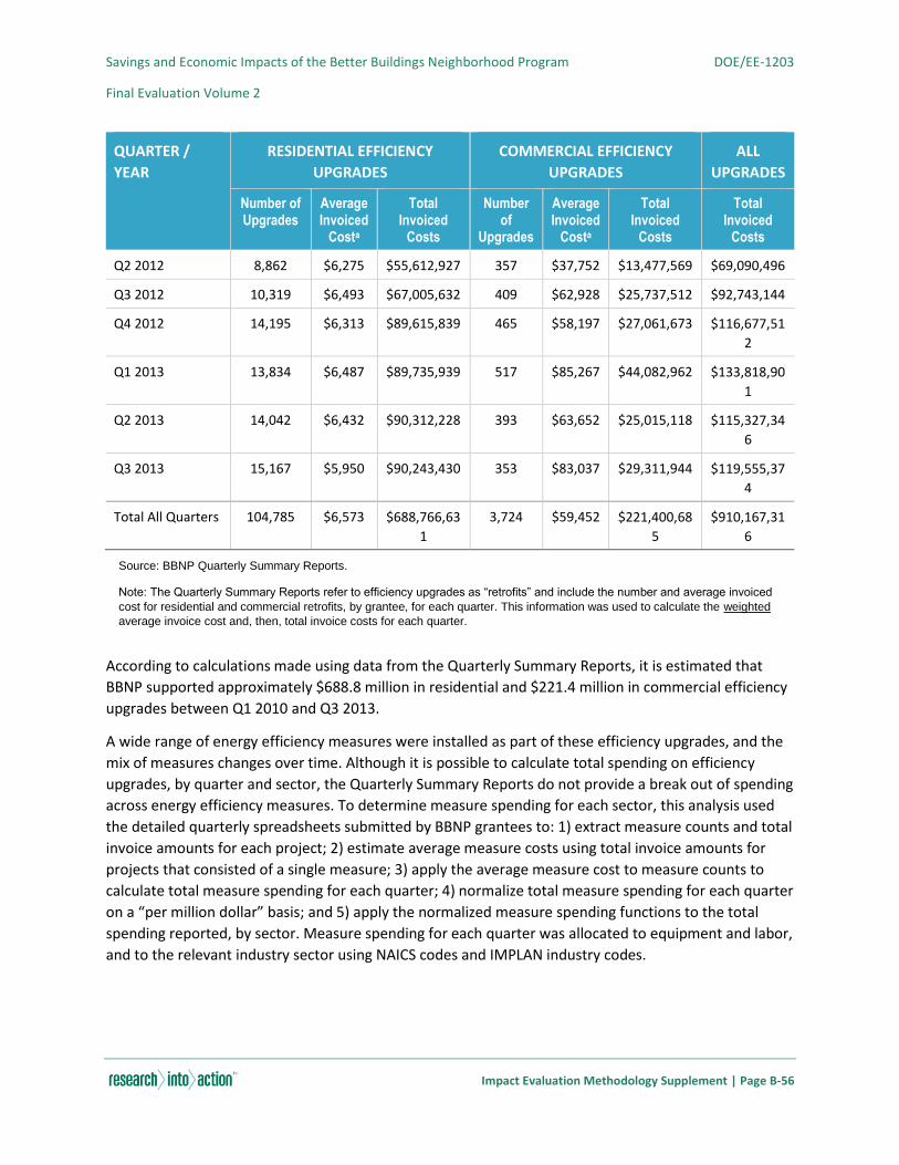
Savings and Economic Impacts of the Better Buildings Neighborhood Program DOE/EE-1203
Final Evaluation Volume 2
Impact Evaluation Methodology Supplement | Page B-56
QUARTER /
YEAR
RESIDENTIAL EFFICIENCY
UPGRADES
COMMERCIAL EFFICIENCY
UPGRADES
ALL
UPGRADES
Number of Upgrades
Average Invoiced
Costa
Total Invoiced
Costs
Number of
Upgrades
Average Invoiced
Costa
Total Invoiced
Costs
Total Invoiced
Costs
Q2 2012 8,862 $6,275 $55,612,927 357 $37,752 $13,477,569 $69,090,496
Q3 2012 10,319 $6,493 $67,005,632 409 $62,928 $25,737,512 $92,743,144
Q4 2012 14,195 $6,313 $89,615,839 465 $58,197 $27,061,673 $116,677,51
2
Q1 2013 13,834 $6,487 $89,735,939 517 $85,267 $44,082,962 $133,818,90
1
Q2 2013 14,042 $6,432 $90,312,228 393 $63,652 $25,015,118 $115,327,34
6
Q3 2013 15,167 $5,950 $90,243,430 353 $83,037 $29,311,944 $119,555,37
4
Total All Quarters 104,785 $6,573 $688,766,63
1
3,724 $59,452 $221,400,68
5
$910,167,31
6
Source: BBNP Quarterly Summary Reports.
Note: The Quarterly Summary Reports refer to efficiency upgrades as “retrofits” and include the number and average invoiced
cost for residential and commercial retrofits, by grantee, for each quarter. This information was used to calculate the weighted
average invoice cost and, then, total invoice costs for each quarter.
According to calculations made using data from the Quarterly Summary Reports, it is estimated that
BBNP supported approximately $688.8 million in residential and $221.4 million in commercial efficiency
upgrades between Q1 2010 and Q3 2013.
A wide range of energy efficiency measures were installed as part of these efficiency upgrades, and the
mix of measures changes over time. Although it is possible to calculate total spending on efficiency
upgrades, by quarter and sector, the Quarterly Summary Reports do not provide a break out of spending
across energy efficiency measures. To determine measure spending for each sector, this analysis used
the detailed quarterly spreadsheets submitted by BBNP grantees to: 1) extract measure counts and total
invoice amounts for each project; 2) estimate average measure costs using total invoice amounts for
projects that consisted of a single measure; 3) apply the average measure cost to measure counts to
calculate total measure spending for each quarter; 4) normalize total measure spending for each quarter
on a “per million dollar” basis; and 5) apply the normalized measure spending functions to the total
spending reported, by sector. Measure spending for each quarter was allocated to equipment and labor,
and to the relevant industry sector using NAICS codes and IMPLAN industry codes.
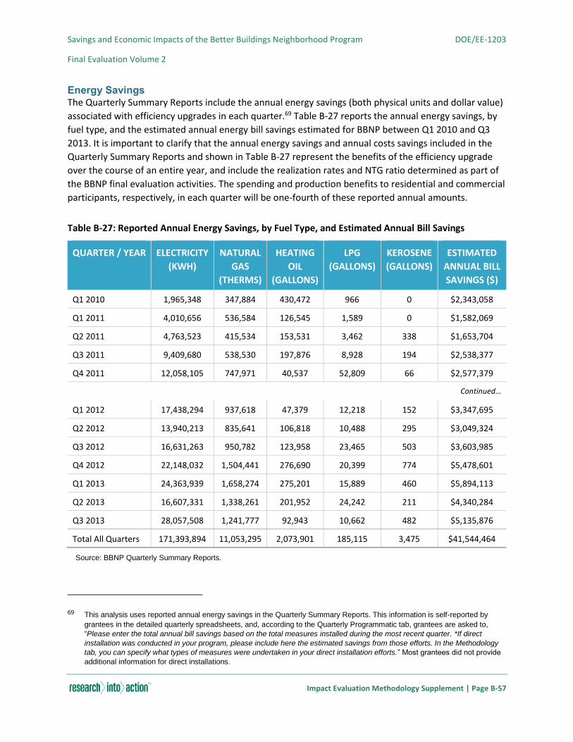
Savings and Economic Impacts of the Better Buildings Neighborhood Program DOE/EE-1203
Final Evaluation Volume 2
Impact Evaluation Methodology Supplement | Page B-57
Energy Savings The Quarterly Summary Reports include the annual energy savings (both physical units and dollar value)
associated with efficiency upgrades in each quarter.69 Table B-27 reports the annual energy savings, by
fuel type, and the estimated annual energy bill savings estimated for BBNP between Q1 2010 and Q3
2013. It is important to clarify that the annual energy savings and annual costs savings included in the
Quarterly Summary Reports and shown in Table B-27 represent the benefits of the efficiency upgrade
over the course of an entire year, and include the realization rates and NTG ratio determined as part of
the BBNP final evaluation activities. The spending and production benefits to residential and commercial
participants, respectively, in each quarter will be one-fourth of these reported annual amounts.
Table B-27: Reported Annual Energy Savings, by Fuel Type, and Estimated Annual Bill Savings
QUARTER / YEAR ELECTRICITY
(KWH)
NATURAL
GAS
(THERMS)
HEATING
OIL
(GALLONS)
LPG
(GALLONS)
KEROSENE
(GALLONS)
ESTIMATED
ANNUAL BILL
SAVINGS ($)
Q1 2010 1,965,348 347,884 430,472 966 0 $2,343,058
Q1 2011 4,010,656 536,584 126,545 1,589 0 $1,582,069
Q2 2011 4,763,523 415,534 153,531 3,462 338 $1,653,704
Q3 2011 9,409,680 538,530 197,876 8,928 194 $2,538,377
Q4 2011 12,058,105 747,971 40,537 52,809 66 $2,577,379
Continued…
Q1 2012 17,438,294 937,618 47,379 12,218 152 $3,347,695
Q2 2012 13,940,213 835,641 106,818 10,488 295 $3,049,324
Q3 2012 16,631,263 950,782 123,958 23,465 503 $3,603,985
Q4 2012 22,148,032 1,504,441 276,690 20,399 774 $5,478,601
Q1 2013 24,363,939 1,658,274 275,201 15,889 460 $5,894,113
Q2 2013 16,607,331 1,338,261 201,952 24,242 211 $4,340,284
Q3 2013 28,057,508 1,241,777 92,943 10,662 482 $5,135,876
Total All Quarters 171,393,894 11,053,295 2,073,901 185,115 3,475 $41,544,464
Source: BBNP Quarterly Summary Reports.
69 This analysis uses reported annual energy savings in the Quarterly Summary Reports. This information is self-reported by
grantees in the detailed quarterly spreadsheets, and, according to the Quarterly Programmatic tab, grantees are asked to,
“Please enter the total annual bill savings based on the total measures installed during the most recent quarter. *If direct
installation was conducted in your program, please include here the estimated savings from those efforts. In the Methodology
tab, you can specify what types of measures were undertaken in your direct installation efforts.” Most grantees did not provide
additional information for direct installations.

Savings and Economic Impacts of the Better Buildings Neighborhood Program DOE/EE-1203
Final Evaluation Volume 2
Impact Evaluation Methodology Supplement | Page B-58
Although the Quarterly Summary Reports include annual energy and bill savings by grantee and quarter,
they do not break out the annual costs savings for residential and commercial sectors. Therefore, this
analysis uses project-level data reported in grantees’ detailed quarterly spreadsheets to allocate total
annual energy bill savings to residential (72.0% of total bill savings) and commercial (28.0%) sectors.
Residential energy bill savings will increase the purchasing power of households on non-energy goods
and services. Energy bill savings for commercial participants will lower their costs of production and, in
the short run, lead to an increase in output. To estimate the changes in output, the distribution of
energy bill savings was estimated across business sectors using the “Principle Building Type” variable in
the grantees’ detailed quarterly spreadsheets.70
The efficiency gains shown in Table B-26 could result in a loss of revenue to utilities and other fuel
providers (producers of heating oil and propane), and this loss of revenue is included in the gross
economic impacts.71 If utilities and other fuel providers had similar economic impact multipliers as other
sectors in the economy, then the energy bill savings in other sectors would roughly cancel out the loss of
revenue in the utility sector. To be consistent with reductions in energy consumption, these revenue
decreases are included in post-installation quarters between Q1 2010 and Q3 2013. They are not,
however, included in annual energy savings impacts beyond this twelve-quarter period.
B.10. LEVERAGING (JAMES WOLF METHODOLOGY AND APPLICATION)
In order to gain a more consistent view of leveraging activities across grantees, DOE asked the research
team to investigate grantees’ use of leveraged funds using the methodology James Wolf reported in “A
Proposed Methodology to Determine the Leveraging Impacts of Technology Deployment Programs”
(Wolf, 2008). This methodology yields a conservative lower-bound estimate of quantity of funds
leveraged.
Wolf specifies a definition for identifying leveraged funds that attempts to account for additionality in
the calculation of leverage. The definition of leveraging DOE articulated in its Funding Opportunity
Announcement (FOA) for BBNP, which includes “building owner contributions, partner contributions, in-
kind contributions, project revenues, other federal funds (including other DOE funds), and state funds,”
is more consistent with popular usage and the methods of previous evaluators (DOE, 2009). The Wolf
methodology is more stringent than was typical of the studies he reviewed and results in fewer funding
sources or monies qualifying as leveraging.
Wolf’s method begins with an investigation of the uses to which the non-program monies are applied.
The method builds on a foundation of logic modeling and distinguishes between program activities,
outputs, and outcomes. The method has two criteria associated with the monies’ usage: 1) that the
monies fund activities, not outputs or outcomes; and 2) that the monies fund what Wolf calls “direct”
70 The detailed quarterly spreadsheets provide grantees with a drop down menu for the Principle Building Type variable. Although
infrequently populated, this approach likely generated a more consistent set of responses.
71 The economic impacts in future post-BBNP years do not include an adjustment for foregone utility revenues.

Savings and Economic Impacts of the Better Buildings Neighborhood Program DOE/EE-1203
Final Evaluation Volume 2
Impact Evaluation Methodology Supplement | Page B-59
program activities – activities that are essential to the program’s logic, and without which one or more
outputs or outcomes would not be attained.
The first criteria (monies for activities) excludes from consideration of leverage funds the monies
participants invest in their upgrades. While reducing participants’ first costs through the provision of
incentives is a program activity, measure installation (with the exception of any direct-install measures;
that is, measures the program installs for free in all applicable participants’ homes) is a program
intermediate outcome, and the energy savings from the measure installations is a final program
outcome.
The second criteria (monies for direct activities) excludes what the author calls “indirect” activities –
activities that are complementary to the program’s objectives but not essential to attaining outputs or
outcomes. Research and development of emerging technologies is an example of an indirect activity for
a program that provides incentives for high efficiency measures. As an example of a qualifying direct
activity, a program might receive funds that enable it to serve an additional neighborhood or town. In
this case, the program is using the funding source to conduct its direct activities in a territory it would
not otherwise serve.
The Wolf methodology also defines three additionality criteria – timing, character of the contribution,
and relative magnitude of funds. The first additionality criteria is timing. If the non-program funding
source was already conducting qualifying activities (that is, direct program activities per the logic model)
and subsequently the program accessed the non-program funding to conduct these activities, then
these non-program funds cannot be considered as leveraged by the program. Indeed, in this case, the
non-program funding source can be considered to have leveraged the program funds. The issue is one of
possible causality: Would the outputs from the direct program activities funded by the non-program
source have occurred in the absence of the program? If the non-program source was active prior to the
program, the causality answer is “no.” As applied to BBNP, this criteria means that none of the program
administrator funds that benefited BBNP participants can be considered as funds that BBNP leveraged, if
those funds were available prior to the launch of the BBNP-funded program. Rather, by this criteria, the
program administrator leveraged BBNP funding.
The second additionality criteria is what Wolf calls “the character of the contribution” made by the
program and the external source of funds. This criteria directs evaluators to consider what both the
program and the non-program funding source contributed to the activities the external funds
supported, including non-financial support like staff time and expertise. As with the consideration of
timing, this consideration fundamentally seeks to determine likely causality: would the activities the
non-program funding supported have occurred in the absence of the program or was the program’s
contribution instrumental in allowing those activities to occur.
The third additionality criteria assesses the relative magnitude of funds. If the amount of non-program
funds is disproportionately greater than the program funds for the activity, then it seems unlikely that
the program elicited the non-program funding; the methodology calls on the evaluator to make a
judgment call as to whether leveraging occurred.
The author discusses, but does not specify in the criteria, the treatment of inter-governmental transfers.
We exclude inter-governmental transfers of funds from its estimation on the following basis:

Savings and Economic Impacts of the Better Buildings Neighborhood Program DOE/EE-1203
Final Evaluation Volume 2
Impact Evaluation Methodology Supplement | Page B-60
Leveraging has become an important issue for government programs as the current political climate
(irrespective of partisan politics) favors public-private partnerships, by which taxpayers receive “more
for their money” than they do with projects funded entirely by taxes. Taxpayers receive no more for
their money when two governmental funding streams are combined to fund a set of activities – the
funds are still all derived from taxes. Indeed, if governmental Office B decides to co-fund the activities of
governmental Office A, one might wonder what Office B has now left unfunded and thus undone.
Taxpayers are likely to have differing opinions on the relative importance of the co-funded activity of
Office A and the resulting unfunded/undone activity of Office B.
Wolf suggests applying the steps of his methodology in succession for each funding source used by the
program. Thus, the evaluator would explore for each funding source the activity or activities funded, the
activity status as direct or indirect, the timing of each source compared to program start, the character
of the contribution, and the relative magnitude of each source compared to program funds.
We developed an in-depth interview guide (see Appendix L) to obtain the information required by the
Wolf methodology and interviewed 15 grantees that reported leveraged funds collectively comprising
78% of all funds grantees reported to DOE as leveraged. We conducted the interviews, lasting about
one-half hour in length, between September 2013 and January 2014. We analyzed the data according to
Wolf’s method to identify amount of leveraged funds.
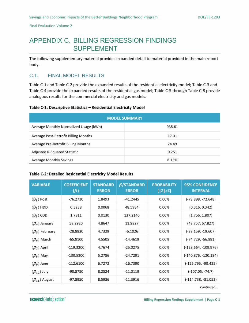
Savings and Economic Impacts of the Better Buildings Neighborhood Program DOE/EE-1203
Final Evaluation Volume 2
Billing Regression Findings Supplement | Page C-1
APPENDIX C. BILLING REGRESSION FINDINGS
SUPPLEMENT
The following supplementary material provides expanded detail to material provided in the main report
body.
C.1. FINAL MODEL RESULTS
Table C-1 and Table C-2 provide the expanded results of the residential electricity model; Table C-3 and
Table C-4 provide the expanded results of the residential gas model; Table C-5 through Table C-8 provide
analogous results for the commercial electricity and gas models.
Table C-1: Descriptive Statistics – Residential Electricity Model
MODEL SUMMARY
Average Monthly Normalized Usage (kWh) 938.61
Average Post-Retrofit Billing Months 17.01
Average Pre-Retrofit Billing Months 24.49
Adjusted R-Squared Statistic 0.251
Average Monthly Savings 8.13%
Table C-2: Detailed Residential Electricity Model Results
VARIABLE COEFFICIENT
(𝜷)
STANDARD
ERROR
𝜷/STANDARD
ERROR
PROBABILITY
[|Z|>Z]
95% CONFIDENCE
INTERVAL
(𝛃𝟏) Post -76.2730 1.8493 -41.2445 0.00% (-79.898, -72.648)
(𝛃𝟐) HDD 0.3288 0.0068 48.5984 0.00% (0.316, 0.342)
(𝛃𝟑) CDD 1.7811 0.0130 137.2140 0.00% (1.756, 1.807)
(𝜷𝟒) January 58.2920 4.8647 11.9827 0.00% (48.757, 67.827)
(𝜷𝟓) February -28.8830 4.7329 -6.1026 0.00% (-38.159, -19.607)
(𝜷𝟔) March -65.8100 4.5505 -14.4619 0.00% (-74.729, -56.891)
(𝜷𝟕) April -119.3200 4.7674 -25.0275 0.00% (-128.664, -109.976)
(𝜷𝟖) May -130.5300 5.2786 -24.7291 0.00% (-140.876, -120.184)
(𝜷𝟗) June -112.6100 6.7272 -16.7390 0.00% (-125.795, -99.425)
(𝜷𝟏𝟎) July -90.8750 8.2524 -11.0119 0.00% (-107.05, -74.7)
(𝜷𝟏𝟏) August -97.8950 8.5936 -11.3916 0.00% (-114.738, -81.052)
Continued…
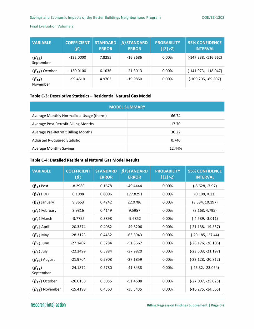
Savings and Economic Impacts of the Better Buildings Neighborhood Program DOE/EE-1203
Final Evaluation Volume 2
Billing Regression Findings Supplement | Page C-2
VARIABLE COEFFICIENT
(𝜷)
STANDARD
ERROR
𝜷/STANDARD
ERROR
PROBABILITY
[|Z|>Z]
95% CONFIDENCE
INTERVAL
(𝜷𝟏𝟐)
September
-132.0000 7.8255 -16.8686 0.00% (-147.338, -116.662)
(𝜷𝟏𝟑) October -130.0100 6.1036 -21.3013 0.00% (-141.973, -118.047)
(𝜷𝟏𝟒)
November
-99.4510 4.9763 -19.9850 0.00% (-109.205, -89.697)
Table C-3: Descriptive Statistics – Residential Natural Gas Model
MODEL SUMMARY
Average Monthly Normalized Usage (therm) 66.74
Average Post-Retrofit Billing Months 17.70
Average Pre-Retrofit Billing Months 30.22
Adjusted R-Squared Statistic 0.740
Average Monthly Savings 12.44%
Table C-4: Detailed Residential Natural Gas Model Results
VARIABLE COEFFICIENT
(𝜷)
STANDARD
ERROR
𝜷/STANDARD
ERROR
PROBABILITY
[|Z|>Z]
95% CONFIDENCE
INTERVAL
(𝛃𝟏) Post -8.2989 0.1678 -49.4444 0.00% (-8.628, -7.97)
(𝛃𝟐) HDD 0.1088 0.0006 177.8291 0.00% (0.108, 0.11)
(𝛃𝟑) January 9.3653 0.4242 22.0786 0.00% (8.534, 10.197)
(𝜷𝟒) February 3.9816 0.4149 9.5957 0.00% (3.168, 4.795)
(𝜷𝟓) March -3.7755 0.3898 -9.6852 0.00% (-4.539, -3.011)
(𝜷𝟔) April -20.3374 0.4082 -49.8206 0.00% (-21.138, -19.537)
(𝜷𝟕) May -28.3123 0.4452 -63.5943 0.00% (-29.185, -27.44)
(𝜷𝟖) June -27.1407 0.5284 -51.3667 0.00% (-28.176, -26.105)
(𝜷𝟗) July -22.3499 0.5884 -37.9820 0.00% (-23.503, -21.197)
(𝜷𝟏𝟎) August -21.9704 0.5908 -37.1859 0.00% (-23.128, -20.812)
(𝜷𝟏𝟏)
September
-24.1872 0.5780 -41.8438 0.00% (-25.32, -23.054)
(𝜷𝟏𝟐) October -26.0158 0.5055 -51.4608 0.00% (-27.007, -25.025)
(𝜷𝟏𝟑) November -15.4198 0.4363 -35.3435 0.00% (-16.275, -14.565)
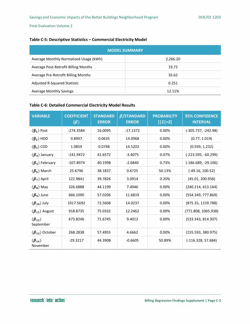
Savings and Economic Impacts of the Better Buildings Neighborhood Program DOE/EE-1203
Final Evaluation Volume 2
Billing Regression Findings Supplement | Page C-3
Table C-5: Descriptive Statistics – Commercial Electricity Model
MODEL SUMMARY
Average Monthly Normalized Usage (kWh) 2,266.20
Average Post-Retrofit Billing Months 19.72
Average Pre-Retrofit Billing Months 35.62
Adjusted R-Squared Statistic 0.251
Average Monthly Savings 12.11%
Table C-6: Detailed Commercial Electricity Model Results
VARIABLE COEFFICIENT
(𝜷)
STANDARD
ERROR
𝜷/STANDARD
ERROR
PROBABILITY
[|Z|>Z]
95% CONFIDENCE
INTERVAL
(𝛃𝟏) Post -274.3584 16.0095 -17.1372 0.00% (-305.737, -242.98)
(𝛃𝟐) HDD 0.8947 0.0635 14.0968 0.00% (0.77, 1.019)
(𝛃𝟑) CDD 1.0859 0.0748 14.5202 0.00% (0.939, 1.232)
(𝜷𝟒) January -141.9472 41.6572 -3.4075 0.07% (-223.595, -60.299)
(𝜷𝟓) February -107.8974 40.1998 -2.6840 0.73% (-186.689, -29.106)
(𝜷𝟔) March 25.6796 38.1837 0.6725 50.13% (-49.16, 100.52)
(𝜷𝟕) April 122.9841 39.7826 3.0914 0.20% (45.01, 200.958)
(𝜷𝟖) May 326.6888 44.1199 7.4046 0.00% (240.214, 413.164)
(𝜷𝟗) June 666.1090 57.0206 11.6819 0.00% (554.349, 777.869)
(𝜷𝟏𝟎) July 1017.5692 72.5608 14.0237 0.00% (875.35, 1159.788)
(𝜷𝟏𝟏) August 918.8735 75.0332 12.2462 0.00% (771.808, 1065.938)
(𝜷𝟏𝟐)
September
673.8246 71.6745 9.4012 0.00% (533.343, 814.307)
(𝜷𝟏𝟑) October 268.2838 57.4955 4.6662 0.00% (155.593, 380.975)
(𝜷𝟏𝟒)
November
-29.3217 44.3908 -0.6605 50.89% (-116.328, 57.684)
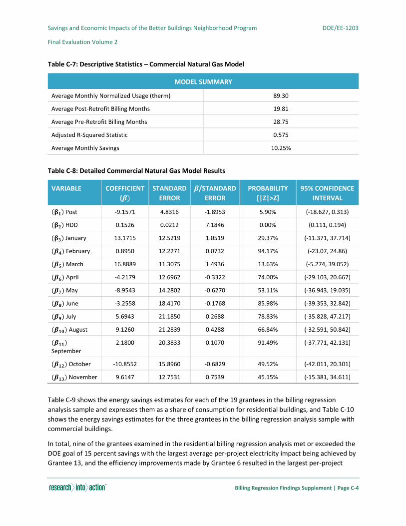
Savings and Economic Impacts of the Better Buildings Neighborhood Program DOE/EE-1203
Final Evaluation Volume 2
Billing Regression Findings Supplement | Page C-4
Table C-7: Descriptive Statistics – Commercial Natural Gas Model
MODEL SUMMARY
Average Monthly Normalized Usage (therm) 89.30
Average Post-Retrofit Billing Months 19.81
Average Pre-Retrofit Billing Months 28.75
Adjusted R-Squared Statistic 0.575
Average Monthly Savings 10.25%
Table C-8: Detailed Commercial Natural Gas Model Results
VARIABLE COEFFICIENT
(𝜷)
STANDARD
ERROR
𝜷/STANDARD
ERROR
PROBABILITY
[|Z|>Z]
95% CONFIDENCE
INTERVAL
(𝛃𝟏) Post -9.1571 4.8316 -1.8953 5.90% (-18.627, 0.313)
(𝛃𝟐) HDD 0.1526 0.0212 7.1846 0.00% (0.111, 0.194)
(𝛃𝟑) January 13.1715 12.5219 1.0519 29.37% (-11.371, 37.714)
(𝜷𝟒) February 0.8950 12.2271 0.0732 94.17% (-23.07, 24.86)
(𝜷𝟓) March 16.8889 11.3075 1.4936 13.63% (-5.274, 39.052)
(𝜷𝟔) April -4.2179 12.6962 -0.3322 74.00% (-29.103, 20.667)
(𝜷𝟕) May -8.9543 14.2802 -0.6270 53.11% (-36.943, 19.035)
(𝜷𝟖) June -3.2558 18.4170 -0.1768 85.98% (-39.353, 32.842)
(𝜷𝟗) July 5.6943 21.1850 0.2688 78.83% (-35.828, 47.217)
(𝜷𝟏𝟎) August 9.1260 21.2839 0.4288 66.84% (-32.591, 50.842)
(𝜷𝟏𝟏)
September
2.1800 20.3833 0.1070 91.49% (-37.771, 42.131)
(𝜷𝟏𝟐) October -10.8552 15.8960 -0.6829 49.52% (-42.011, 20.301)
(𝜷𝟏𝟑) November 9.6147 12.7531 0.7539 45.15% (-15.381, 34.611)
Table C-9 shows the energy savings estimates for each of the 19 grantees in the billing regression
analysis sample and expresses them as a share of consumption for residential buildings, and Table C-10
shows the energy savings estimates for the three grantees in the billing regression analysis sample with
commercial buildings.
In total, nine of the grantees examined in the residential billing regression analysis met or exceeded the
DOE goal of 15 percent savings with the largest average per-project electricity impact being achieved by
Grantee 13, and the efficiency improvements made by Grantee 6 resulted in the largest per-project
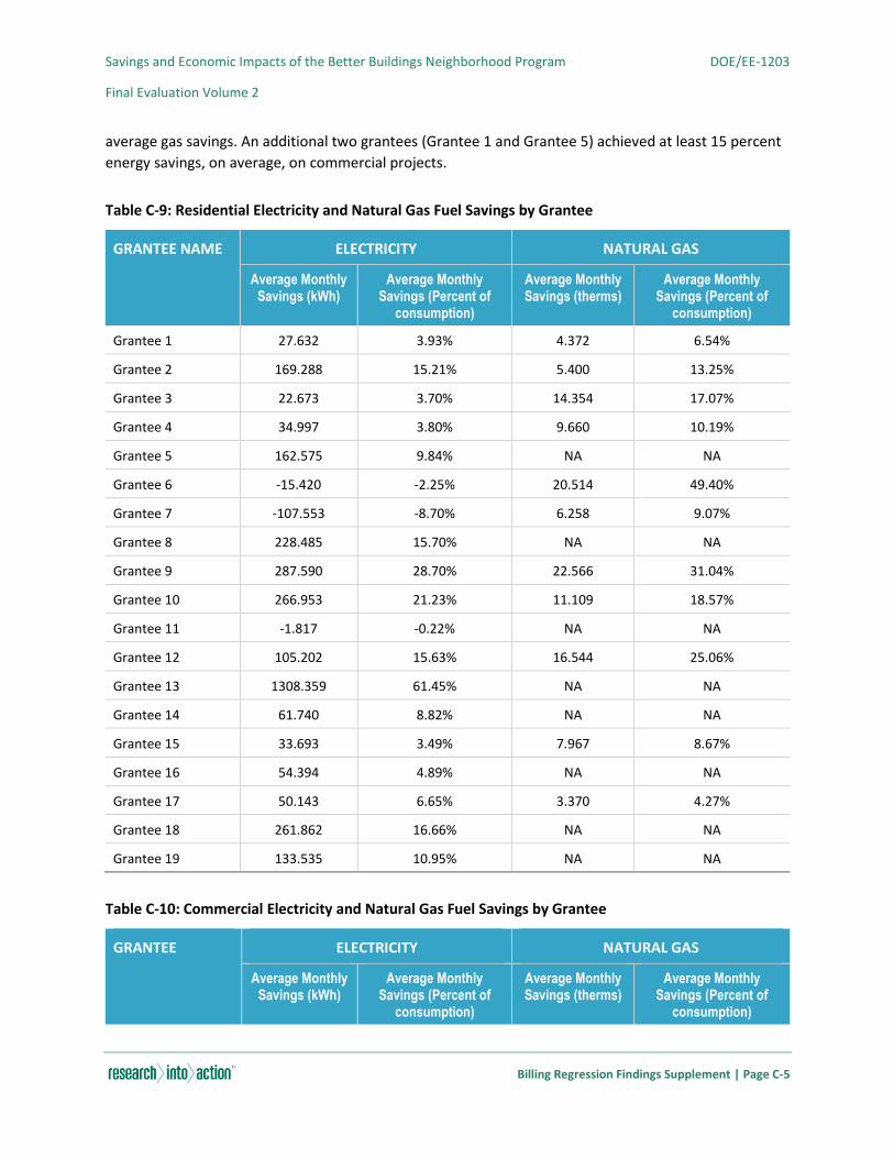
Savings and Economic Impacts of the Better Buildings Neighborhood Program DOE/EE-1203
Final Evaluation Volume 2
Billing Regression Findings Supplement | Page C-5
average gas savings. An additional two grantees (Grantee 1 and Grantee 5) achieved at least 15 percent
energy savings, on average, on commercial projects.
Table C-9: Residential Electricity and Natural Gas Fuel Savings by Grantee
GRANTEE NAME ELECTRICITY NATURAL GAS
Average Monthly Savings (kWh)
Average Monthly Savings (Percent of
consumption)
Average Monthly Savings (therms)
Average Monthly Savings (Percent of
consumption)
Grantee 1 27.632 3.93% 4.372 6.54%
Grantee 2 169.288 15.21% 5.400 13.25%
Grantee 3 22.673 3.70% 14.354 17.07%
Grantee 4 34.997 3.80% 9.660 10.19%
Grantee 5 162.575 9.84% NA NA
Grantee 6 -15.420 -2.25% 20.514 49.40%
Grantee 7 -107.553 -8.70% 6.258 9.07%
Grantee 8 228.485 15.70% NA NA
Grantee 9 287.590 28.70% 22.566 31.04%
Grantee 10 266.953 21.23% 11.109 18.57%
Grantee 11 -1.817 -0.22% NA NA
Grantee 12 105.202 15.63% 16.544 25.06%
Grantee 13 1308.359 61.45% NA NA
Grantee 14 61.740 8.82% NA NA
Grantee 15 33.693 3.49% 7.967 8.67%
Grantee 16 54.394 4.89% NA NA
Grantee 17 50.143 6.65% 3.370 4.27%
Grantee 18 261.862 16.66% NA NA
Grantee 19 133.535 10.95% NA NA
Table C-10: Commercial Electricity and Natural Gas Fuel Savings by Grantee
GRANTEE ELECTRICITY NATURAL GAS
Average Monthly Savings (kWh)
Average Monthly Savings (Percent of
consumption)
Average Monthly Savings (therms)
Average Monthly Savings (Percent of
consumption)
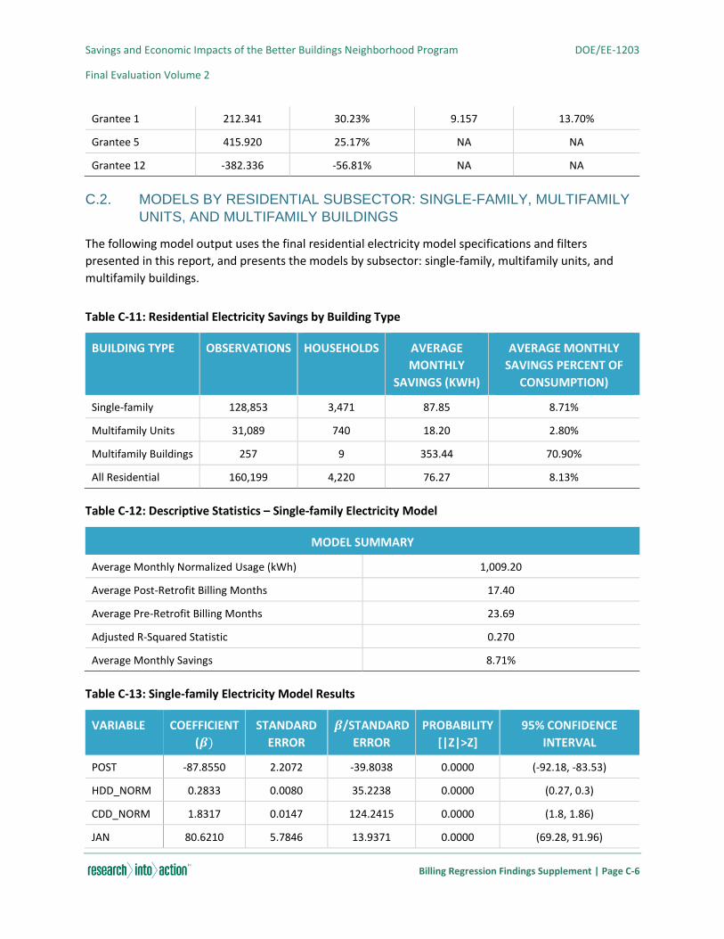
Savings and Economic Impacts of the Better Buildings Neighborhood Program DOE/EE-1203
Final Evaluation Volume 2
Billing Regression Findings Supplement | Page C-6
Grantee 1 212.341 30.23% 9.157 13.70%
Grantee 5 415.920 25.17% NA NA
Grantee 12 -382.336 -56.81% NA NA
C.2. MODELS BY RESIDENTIAL SUBSECTOR: SINGLE-FAMILY, MULTIFAMILY
UNITS, AND MULTIFAMILY BUILDINGS
The following model output uses the final residential electricity model specifications and filters
presented in this report, and presents the models by subsector: single-family, multifamily units, and
multifamily buildings.
Table C-11: Residential Electricity Savings by Building Type
BUILDING TYPE OBSERVATIONS HOUSEHOLDS AVERAGE
MONTHLY
SAVINGS (KWH)
AVERAGE MONTHLY
SAVINGS PERCENT OF
CONSUMPTION)
Single-family 128,853 3,471 87.85 8.71%
Multifamily Units 31,089 740 18.20 2.80%
Multifamily Buildings 257 9 353.44 70.90%
All Residential 160,199 4,220 76.27 8.13%
Table C-12: Descriptive Statistics – Single-family Electricity Model
MODEL SUMMARY
Average Monthly Normalized Usage (kWh) 1,009.20
Average Post-Retrofit Billing Months 17.40
Average Pre-Retrofit Billing Months 23.69
Adjusted R-Squared Statistic 0.270
Average Monthly Savings 8.71%
Table C-13: Single-family Electricity Model Results
VARIABLE COEFFICIENT
(𝜷)
STANDARD
ERROR
𝜷/STANDARD
ERROR
PROBABILITY
[|Z|>Z]
95% CONFIDENCE
INTERVAL
POST -87.8550 2.2072 -39.8038 0.0000 (-92.18, -83.53)
HDD_NORM 0.2833 0.0080 35.2238 0.0000 (0.27, 0.3)
CDD_NORM 1.8317 0.0147 124.2415 0.0000 (1.8, 1.86)
JAN 80.6210 5.7846 13.9371 0.0000 (69.28, 91.96)
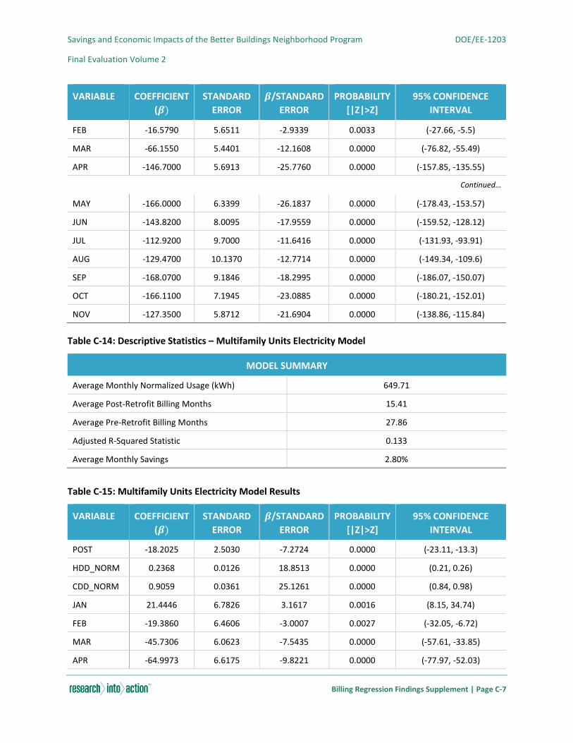
Savings and Economic Impacts of the Better Buildings Neighborhood Program DOE/EE-1203
Final Evaluation Volume 2
Billing Regression Findings Supplement | Page C-7
VARIABLE COEFFICIENT
(𝜷)
STANDARD
ERROR
𝜷/STANDARD
ERROR
PROBABILITY
[|Z|>Z]
95% CONFIDENCE
INTERVAL
FEB -16.5790 5.6511 -2.9339 0.0033 (-27.66, -5.5)
MAR -66.1550 5.4401 -12.1608 0.0000 (-76.82, -55.49)
APR -146.7000 5.6913 -25.7760 0.0000 (-157.85, -135.55)
Continued…
MAY -166.0000 6.3399 -26.1837 0.0000 (-178.43, -153.57)
JUN -143.8200 8.0095 -17.9559 0.0000 (-159.52, -128.12)
JUL -112.9200 9.7000 -11.6416 0.0000 (-131.93, -93.91)
AUG -129.4700 10.1370 -12.7714 0.0000 (-149.34, -109.6)
SEP -168.0700 9.1846 -18.2995 0.0000 (-186.07, -150.07)
OCT -166.1100 7.1945 -23.0885 0.0000 (-180.21, -152.01)
NOV -127.3500 5.8712 -21.6904 0.0000 (-138.86, -115.84)
Table C-14: Descriptive Statistics – Multifamily Units Electricity Model
MODEL SUMMARY
Average Monthly Normalized Usage (kWh) 649.71
Average Post-Retrofit Billing Months 15.41
Average Pre-Retrofit Billing Months 27.86
Adjusted R-Squared Statistic 0.133
Average Monthly Savings 2.80%
Table C-15: Multifamily Units Electricity Model Results
VARIABLE COEFFICIENT
(𝜷)
STANDARD
ERROR
𝜷/STANDARD
ERROR
PROBABILITY
[|Z|>Z]
95% CONFIDENCE
INTERVAL
POST -18.2025 2.5030 -7.2724 0.0000 (-23.11, -13.3)
HDD_NORM 0.2368 0.0126 18.8513 0.0000 (0.21, 0.26)
CDD_NORM 0.9059 0.0361 25.1261 0.0000 (0.84, 0.98)
JAN 21.4446 6.7826 3.1617 0.0016 (8.15, 34.74)
FEB -19.3860 6.4606 -3.0007 0.0027 (-32.05, -6.72)
MAR -45.7306 6.0623 -7.5435 0.0000 (-57.61, -33.85)
APR -64.9973 6.6175 -9.8221 0.0000 (-77.97, -52.03)
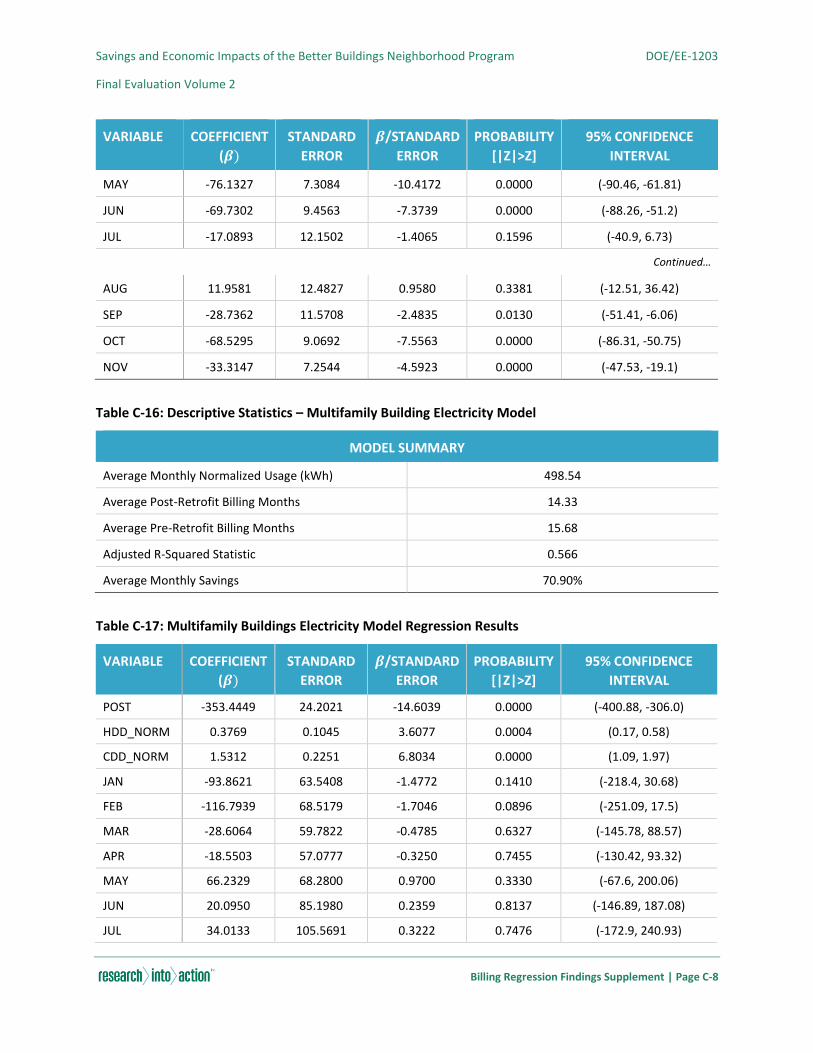
Savings and Economic Impacts of the Better Buildings Neighborhood Program DOE/EE-1203
Final Evaluation Volume 2
Billing Regression Findings Supplement | Page C-8
VARIABLE COEFFICIENT
(𝜷)
STANDARD
ERROR
𝜷/STANDARD
ERROR
PROBABILITY
[|Z|>Z]
95% CONFIDENCE
INTERVAL
MAY -76.1327 7.3084 -10.4172 0.0000 (-90.46, -61.81)
JUN -69.7302 9.4563 -7.3739 0.0000 (-88.26, -51.2)
JUL -17.0893 12.1502 -1.4065 0.1596 (-40.9, 6.73)
Continued…
AUG 11.9581 12.4827 0.9580 0.3381 (-12.51, 36.42)
SEP -28.7362 11.5708 -2.4835 0.0130 (-51.41, -6.06)
OCT -68.5295 9.0692 -7.5563 0.0000 (-86.31, -50.75)
NOV -33.3147 7.2544 -4.5923 0.0000 (-47.53, -19.1)
Table C-16: Descriptive Statistics – Multifamily Building Electricity Model
MODEL SUMMARY
Average Monthly Normalized Usage (kWh) 498.54
Average Post-Retrofit Billing Months 14.33
Average Pre-Retrofit Billing Months 15.68
Adjusted R-Squared Statistic 0.566
Average Monthly Savings 70.90%
Table C-17: Multifamily Buildings Electricity Model Regression Results
VARIABLE COEFFICIENT
(𝜷)
STANDARD
ERROR
𝜷/STANDARD
ERROR
PROBABILITY
[|Z|>Z]
95% CONFIDENCE
INTERVAL
POST -353.4449 24.2021 -14.6039 0.0000 (-400.88, -306.0)
HDD_NORM 0.3769 0.1045 3.6077 0.0004 (0.17, 0.58)
CDD_NORM 1.5312 0.2251 6.8034 0.0000 (1.09, 1.97)
JAN -93.8621 63.5408 -1.4772 0.1410 (-218.4, 30.68)
FEB -116.7939 68.5179 -1.7046 0.0896 (-251.09, 17.5)
MAR -28.6064 59.7822 -0.4785 0.6327 (-145.78, 88.57)
APR -18.5503 57.0777 -0.3250 0.7455 (-130.42, 93.32)
MAY 66.2329 68.2800 0.9700 0.3330 (-67.6, 200.06)
JUN 20.0950 85.1980 0.2359 0.8137 (-146.89, 187.08)
JUL 34.0133 105.5691 0.3222 0.7476 (-172.9, 240.93)
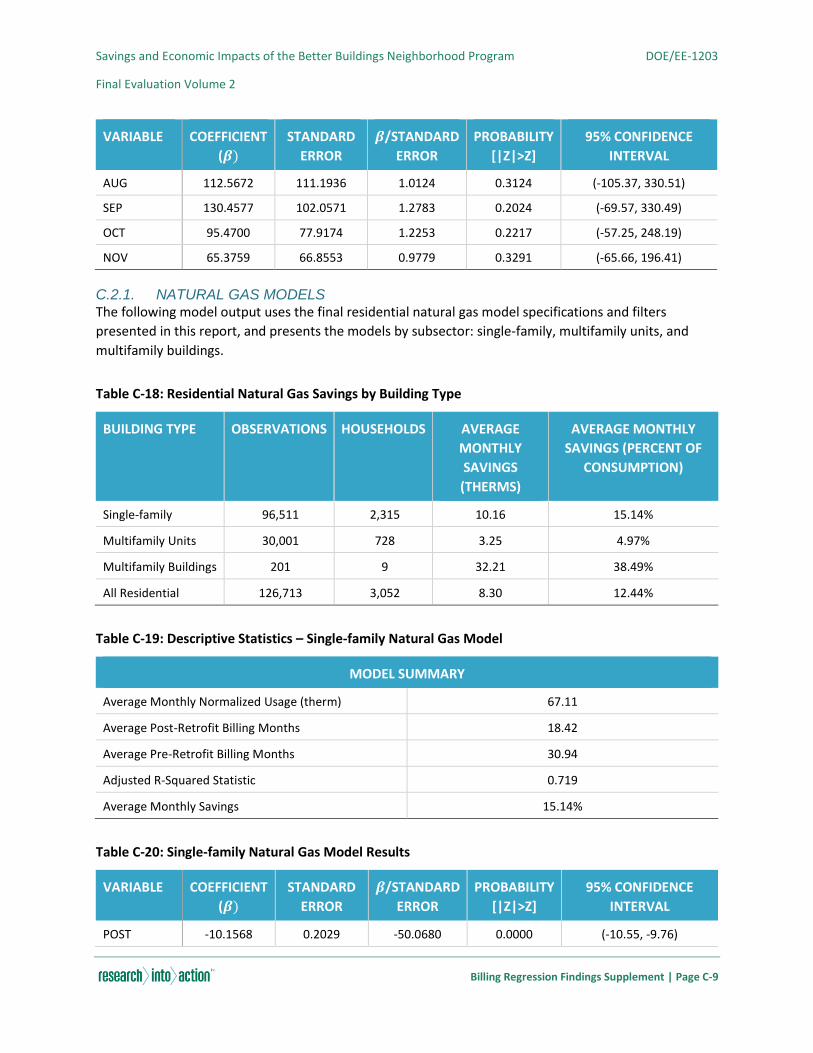
Savings and Economic Impacts of the Better Buildings Neighborhood Program DOE/EE-1203
Final Evaluation Volume 2
Billing Regression Findings Supplement | Page C-9
VARIABLE COEFFICIENT
(𝜷)
STANDARD
ERROR
𝜷/STANDARD
ERROR
PROBABILITY
[|Z|>Z]
95% CONFIDENCE
INTERVAL
AUG 112.5672 111.1936 1.0124 0.3124 (-105.37, 330.51)
SEP 130.4577 102.0571 1.2783 0.2024 (-69.57, 330.49)
OCT 95.4700 77.9174 1.2253 0.2217 (-57.25, 248.19)
NOV 65.3759 66.8553 0.9779 0.3291 (-65.66, 196.41)
C.2.1. NATURAL GAS MODELS The following model output uses the final residential natural gas model specifications and filters
presented in this report, and presents the models by subsector: single-family, multifamily units, and
multifamily buildings.
Table C-18: Residential Natural Gas Savings by Building Type
BUILDING TYPE OBSERVATIONS HOUSEHOLDS AVERAGE
MONTHLY
SAVINGS
(THERMS)
AVERAGE MONTHLY
SAVINGS (PERCENT OF
CONSUMPTION)
Single-family 96,511 2,315 10.16 15.14%
Multifamily Units 30,001 728 3.25 4.97%
Multifamily Buildings 201 9 32.21 38.49%
All Residential 126,713 3,052 8.30 12.44%
Table C-19: Descriptive Statistics – Single-family Natural Gas Model
MODEL SUMMARY
Average Monthly Normalized Usage (therm) 67.11
Average Post-Retrofit Billing Months 18.42
Average Pre-Retrofit Billing Months 30.94
Adjusted R-Squared Statistic 0.719
Average Monthly Savings 15.14%
Table C-20: Single-family Natural Gas Model Results
VARIABLE COEFFICIENT
(𝜷)
STANDARD
ERROR
𝜷/STANDARD
ERROR
PROBABILITY
[|Z|>Z]
95% CONFIDENCE
INTERVAL
POST -10.1568 0.2029 -50.0680 0.0000 (-10.55, -9.76)

Savings and Economic Impacts of the Better Buildings Neighborhood Program DOE/EE-1203
Final Evaluation Volume 2
Billing Regression Findings Supplement | Page C-10
VARIABLE COEFFICIENT
(𝜷)
STANDARD
ERROR
𝜷/STANDARD
ERROR
PROBABILITY
[|Z|>Z]
95% CONFIDENCE
INTERVAL
HDD_NORM 0.1080 0.0007 150.4790 0.0000 (0.11, 0.11)
JAN 10.2866 0.5041 20.4075 0.0000 (9.3, 11.27)
FEB 3.9302 0.4968 7.9103 0.0000 (2.96, 4.9)
MAR -3.0883 0.4659 -6.6280 0.0000 (-4, -2.18)
APR -20.4277 0.4860 -42.0364 0.0000 (-21.38, -19.48)
MAY -29.1724 0.5299 -55.0562 0.0000 (-30.21, -28.13)
Continued…
JUN -29.0815 0.6185 -47.0225 0.0000 (-30.29, -27.87)
JUL -25.3076 0.6828 -37.0640 0.0000 (-26.65, -23.97)
AUG -25.3533 0.6824 -37.1528 0.0000 (-26.69, -24.02)
SEP -26.8762 0.6687 -40.1890 0.0000 (-28.19, -25.57)
OCT -26.3559 0.5890 -44.7444 0.0000 (-27.51, -25.2)
NOV -15.5407 0.5148 -30.1853 0.0000 (-16.55, -14.53)
Table C-21: Descriptive Statistics – Multifamily Units Natural Gas Model
MODEL SUMMARY
Average Monthly Normalized Usage (therm) 65.43
Average Post-Retrofit Billing Months 15.42
Average Pre-Retrofit Billing Months 28.00
Adjusted R-Squared Statistic 0.825
Average Monthly Savings 4.97%
Table C-22: Multifamily Units Natural Gas Model Results
VARIABLE COEFFICIENT
(𝜷)
STANDARD
ERROR
𝜷/STANDARD
ERROR
PROBABILITY
[|Z|>Z]
95% CONFIDENCE
INTERVAL
POST -3.2549 0.2692 -12.0901 0.0000 (-3.78, -2.73)
HDD_NORM 0.1260 0.0012 104.1483 0.0000 (0.12, 0.13)
JAN 3.7425 0.7180 5.2123 0.0000 (2.34, 5.15)
FEB 2.5690 0.6835 3.7586 0.0002 (1.23, 3.91)
MAR -6.0750 0.6422 -9.4599 0.0000 (-7.33, -4.82)
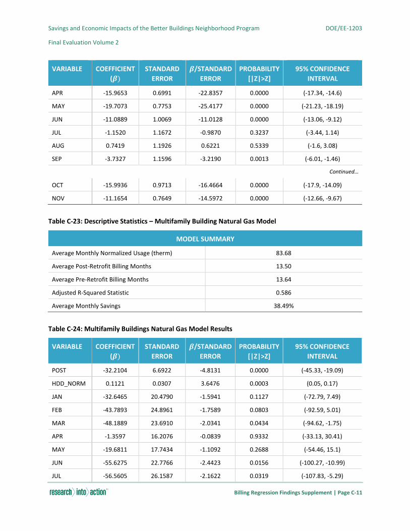
Savings and Economic Impacts of the Better Buildings Neighborhood Program DOE/EE-1203
Final Evaluation Volume 2
Billing Regression Findings Supplement | Page C-11
VARIABLE COEFFICIENT
(𝜷)
STANDARD
ERROR
𝜷/STANDARD
ERROR
PROBABILITY
[|Z|>Z]
95% CONFIDENCE
INTERVAL
APR -15.9653 0.6991 -22.8357 0.0000 (-17.34, -14.6)
MAY -19.7073 0.7753 -25.4177 0.0000 (-21.23, -18.19)
JUN -11.0889 1.0069 -11.0128 0.0000 (-13.06, -9.12)
JUL -1.1520 1.1672 -0.9870 0.3237 (-3.44, 1.14)
AUG 0.7419 1.1926 0.6221 0.5339 (-1.6, 3.08)
SEP -3.7327 1.1596 -3.2190 0.0013 (-6.01, -1.46)
Continued…
OCT -15.9936 0.9713 -16.4664 0.0000 (-17.9, -14.09)
NOV -11.1654 0.7649 -14.5972 0.0000 (-12.66, -9.67)
Table C-23: Descriptive Statistics – Multifamily Building Natural Gas Model
MODEL SUMMARY
Average Monthly Normalized Usage (therm) 83.68
Average Post-Retrofit Billing Months 13.50
Average Pre-Retrofit Billing Months 13.64
Adjusted R-Squared Statistic 0.586
Average Monthly Savings 38.49%
Table C-24: Multifamily Buildings Natural Gas Model Results
VARIABLE COEFFICIENT
(𝜷)
STANDARD
ERROR
𝜷/STANDARD
ERROR
PROBABILITY
[|Z|>Z]
95% CONFIDENCE
INTERVAL
POST -32.2104 6.6922 -4.8131 0.0000 (-45.33, -19.09)
HDD_NORM 0.1121 0.0307 3.6476 0.0003 (0.05, 0.17)
JAN -32.6465 20.4790 -1.5941 0.1127 (-72.79, 7.49)
FEB -43.7893 24.8961 -1.7589 0.0803 (-92.59, 5.01)
MAR -48.1889 23.6910 -2.0341 0.0434 (-94.62, -1.75)
APR -1.3597 16.2076 -0.0839 0.9332 (-33.13, 30.41)
MAY -19.6811 17.7434 -1.1092 0.2688 (-54.46, 15.1)
JUN -55.6275 22.7766 -2.4423 0.0156 (-100.27, -10.99)
JUL -56.5605 26.1587 -2.1622 0.0319 (-107.83, -5.29)
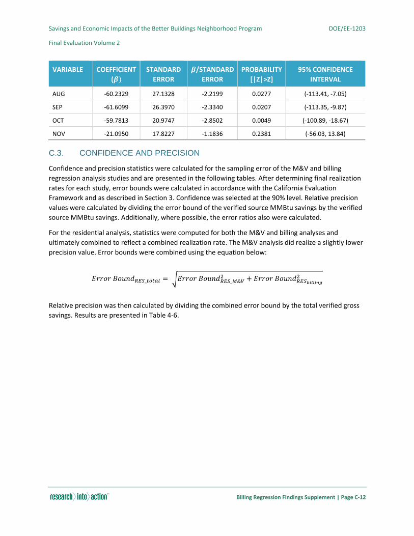
Savings and Economic Impacts of the Better Buildings Neighborhood Program DOE/EE-1203
Final Evaluation Volume 2
Billing Regression Findings Supplement | Page C-12
VARIABLE COEFFICIENT
(𝜷)
STANDARD
ERROR
𝜷/STANDARD
ERROR
PROBABILITY
[|Z|>Z]
95% CONFIDENCE
INTERVAL
AUG -60.2329 27.1328 -2.2199 0.0277 (-113.41, -7.05)
SEP -61.6099 26.3970 -2.3340 0.0207 (-113.35, -9.87)
OCT -59.7813 20.9747 -2.8502 0.0049 (-100.89, -18.67)
NOV -21.0950 17.8227 -1.1836 0.2381 (-56.03, 13.84)
C.3. CONFIDENCE AND PRECISION
Confidence and precision statistics were calculated for the sampling error of the M&V and billing
regression analysis studies and are presented in the following tables. After determining final realization
rates for each study, error bounds were calculated in accordance with the California Evaluation
Framework and as described in Section 3. Confidence was selected at the 90% level. Relative precision
values were calculated by dividing the error bound of the verified source MMBtu savings by the verified
source MMBtu savings. Additionally, where possible, the error ratios also were calculated.
For the residential analysis, statistics were computed for both the M&V and billing analyses and
ultimately combined to reflect a combined realization rate. The M&V analysis did realize a slightly lower
precision value. Error bounds were combined using the equation below:
𝐸𝑟𝑟𝑜𝑟 𝐵𝑜𝑢𝑛𝑑𝑅𝐸𝑆_𝑡𝑜𝑡𝑎𝑙 = √𝐸𝑟𝑟𝑜𝑟 𝐵𝑜𝑢𝑛𝑑𝑅𝐸𝑆_𝑀&𝑉2 + 𝐸𝑟𝑟𝑜𝑟 𝐵𝑜𝑢𝑛𝑑𝑅𝐸𝑆𝑏𝑖𝑙𝑙𝑖𝑛𝑔
2
Relative precision was then calculated by dividing the combined error bound by the total verified gross
savings. Results are presented in Table 4-6.
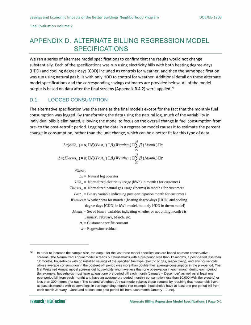
Savings and Economic Impacts of the Better Buildings Neighborhood Program DOE/EE-1203
Final Evaluation Volume 2
Alternate Billing Regression Model Specifications | Page D-1
APPENDIX D. ALTERNATE BILLING REGRESSION MODEL
SPECIFICATIONS
We ran a series of alternate model specifications to confirm that the results would not change
substantially. Each of the specifications was run using electricity bills with both heating degree-days
(HDD) and cooling degree-days (CDD) included as controls for weather, and then the same specification
was run using natural gas bills with only HDD to control for weather. Additional detail on these alternate
model specifications and the corresponding savings estimates are provided below. All of the model
output is based on data after the final screens (Appendix B.4.2) were applied.72
D.1. LOGGED CONSUMPTION
The alternative specification was the same as the final models except for the fact that the monthly fuel
consumption was logged. By transforming the data using the natural log, much of the variability in
individual bills is eliminated, allowing the model to focus on the overall change in fuel consumption from
pre- to the post-retrofit period. Logging the data in a regression model causes it to estimate the percent
change in consumption, rather than the unit change, which can be a better fit for this type of data.
72 In order to increase the sample size, the output for the last three model specifications are based on more conservative
screens. The Normalized Annual model screens out households with a pre-period less than 12 months, a post-period less than
12 months, households with no installed savings of the specified fuel type (electric or gas, respectively), and any households
whose average consumption in the post-retrofit period was more than double their average consumption in the pre-period. The
first Weighted Annual model screens out households who have less than one observation in each month during each period
(for example, households must have at least one pre-period bill each month (January – December) as well as at least one
post-period bill from each month) and have an average pre-period monthly consumption less than 10,000 kWh (for electric) or
less than 300 therms (for gas). The second Weighted Annual model relaxes these screens by requiring that households have
at least six months with observations in corresponding months (for example, households have at least one pre-period bill from
each month January – June and at least one post-period bill from each month January – June).
Ln(kWhi,t ) = ai + b1(Posti,t )+ b2 (Weathert )+ b j (Montht )j=3
13
å +e
Ln(Thermsi,t ) = ai + b1(Posti,t )+ b2 (Weathert )+ b j (Montht )j=3
13
å +e
Where :
Ln = Natural log operator
kWhi,t = Normalized electricity usage (kWh) in month t for customer i
Thermsi,t = Normalized natural gas usage (therms) in month t for customer i
Posti,t = Binary variable indicating post-participation month for customer i
Weathert= Weather data for month t (heating degree-days [HDD] and cooling
degree-days [CDD] in kWh model, but only HDD in therm model)
Montht = Set of binary variables indicating whether or not billing month t is
January, February, March, etc.
ai = Customer-specific constant
e = Regression residual
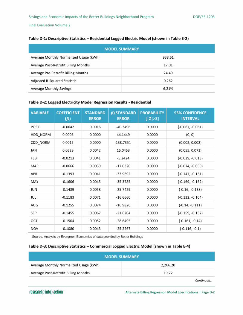
Savings and Economic Impacts of the Better Buildings Neighborhood Program DOE/EE-1203
Final Evaluation Volume 2
Alternate Billing Regression Model Specifications | Page D-2
Table D-1: Descriptive Statistics – Residential Logged Electric Model (shown in Table E-2)
MODEL SUMMARY
Average Monthly Normalized Usage (kWh) 938.61
Average Post-Retrofit Billing Months 17.01
Average Pre-Retrofit Billing Months 24.49
Adjusted R-Squared Statistic 0.262
Average Monthly Savings 6.21%
Table D-2: Logged Electricity Model Regression Results - Residential
VARIABLE COEFFICIENT
(𝜷)
STANDARD
ERROR
𝜷/STANDARD
ERROR
PROBABILITY
[|Z|>Z]
95% CONFIDENCE
INTERVAL
POST -0.0642 0.0016 -40.3496 0.0000 (-0.067, -0.061)
HDD_NORM 0.0003 0.0000 44.1449 0.0000 (0, 0)
CDD_NORM 0.0015 0.0000 138.7351 0.0000 (0.002, 0.002)
JAN 0.0629 0.0042 15.0453 0.0000 (0.055, 0.071)
FEB -0.0213 0.0041 -5.2424 0.0000 (-0.029, -0.013)
MAR -0.0666 0.0039 -17.0320 0.0000 (-0.074, -0.059)
APR -0.1393 0.0041 -33.9692 0.0000 (-0.147, -0.131)
MAY -0.1606 0.0045 -35.3785 0.0000 (-0.169, -0.152)
JUN -0.1489 0.0058 -25.7429 0.0000 (-0.16, -0.138)
JUL -0.1183 0.0071 -16.6660 0.0000 (-0.132, -0.104)
AUG -0.1255 0.0074 -16.9826 0.0000 (-0.14, -0.111)
SEP -0.1455 0.0067 -21.6204 0.0000 (-0.159, -0.132)
OCT -0.1504 0.0052 -28.6495 0.0000 (-0.161, -0.14)
NOV -0.1080 0.0043 -25.2267 0.0000 (-0.116, -0.1)
Source: Analysis by Evergreen Economics of data provided by Better Buildings
Table D-3: Descriptive Statistics – Commercial Logged Electric Model (shown in Table E-4)
MODEL SUMMARY
Average Monthly Normalized Usage (kWh) 2,266.20
Average Post-Retrofit Billing Months 19.72
Continued…

Savings and Economic Impacts of the Better Buildings Neighborhood Program DOE/EE-1203
Final Evaluation Volume 2
Alternate Billing Regression Model Specifications | Page D-3
MODEL SUMMARY
Average Pre-Retrofit Billing Months 35.62
Adjusted R-Squared Statistic 0.220
Average Monthly Savings 14.57%
Table D-4: Logged Electricity Model Regression Results – Commercial
VARIABLE COEFFICIENT
(𝜷)
STANDARD
ERROR
𝜷/STANDARD
ERROR
PROBABILITY
[|Z|>Z]
95% CONFIDENCE
INTERVAL
POST -0.1575 0.0072 -21.8446 0.0000 (-0.172, -0.143)
HDD_NORM 0.0003 0.0000 12.2373 0.0000 (0, 0)
CDD_NORM 0.0005 0.0000 14.5706 0.0000 (0, 0.001)
JAN -0.0607 0.0188 -3.2358 0.0012 (-0.097, -0.024)
FEB -0.0654 0.0181 -3.6115 0.0003 (-0.101, -0.03)
MAR 0.0043 0.0172 0.2506 0.8021 (-0.029, 0.038)
APR 0.0242 0.0179 1.3509 0.1768 (-0.011, 0.059)
MAY 0.0968 0.0199 4.8729 0.0000 (0.058, 0.136)
JUN 0.2410 0.0257 9.3862 0.0000 (0.191, 0.291)
JUL 0.3317 0.0327 10.1521 0.0000 (0.268, 0.396)
AUG 0.3124 0.0338 9.2444 0.0000 (0.246, 0.379)
SEP 0.2366 0.0323 7.3292 0.0000 (0.173, 0.3)
OCT 0.0847 0.0259 3.2707 0.0011 (0.034, 0.135)
NOV -0.0432 0.0200 -2.1593 0.0308 (-0.082, -0.004)
Source: Analysis by Evergreen Economics of data provided by Better Buildings
Table D-5: Descriptive Statistics –Residential Logged Natural Gas Model (shown in Table E-6)
MODEL SUMMARY
Average Monthly Normalized Usage (therm) 66.74
Average Post-Retrofit Billing Months 17.70
Average Pre-Retrofit Billing Months 30.22
Adjusted R-Squared Statistic 0.823
Average Monthly Savings 11.90%
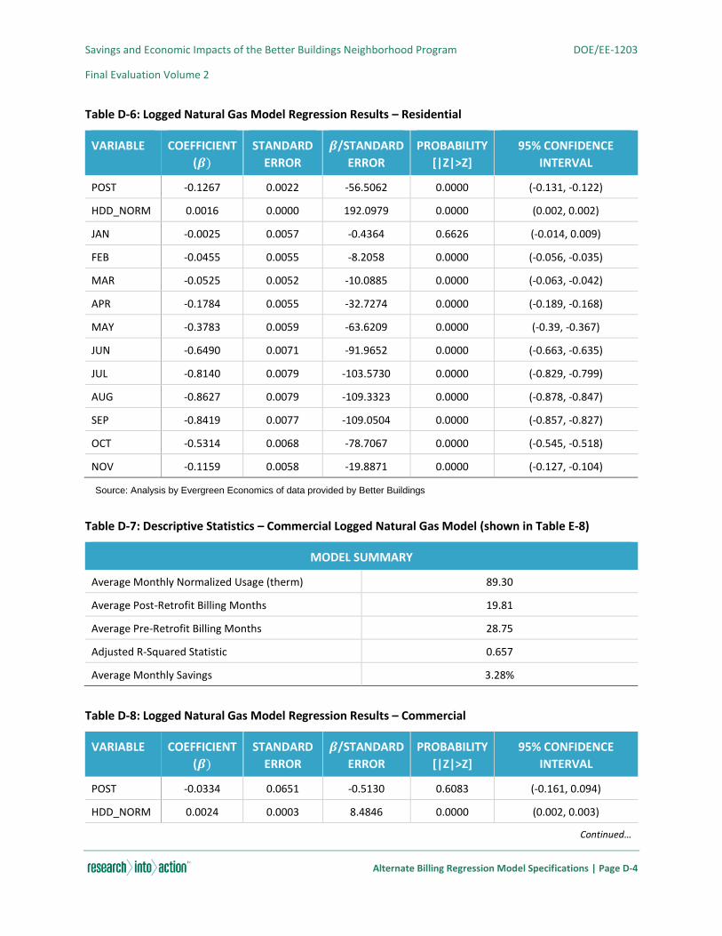
Savings and Economic Impacts of the Better Buildings Neighborhood Program DOE/EE-1203
Final Evaluation Volume 2
Alternate Billing Regression Model Specifications | Page D-4
Table D-6: Logged Natural Gas Model Regression Results – Residential
VARIABLE COEFFICIENT
(𝜷)
STANDARD
ERROR
𝜷/STANDARD
ERROR
PROBABILITY
[|Z|>Z]
95% CONFIDENCE
INTERVAL
POST -0.1267 0.0022 -56.5062 0.0000 (-0.131, -0.122)
HDD_NORM 0.0016 0.0000 192.0979 0.0000 (0.002, 0.002)
JAN -0.0025 0.0057 -0.4364 0.6626 (-0.014, 0.009)
FEB -0.0455 0.0055 -8.2058 0.0000 (-0.056, -0.035)
MAR -0.0525 0.0052 -10.0885 0.0000 (-0.063, -0.042)
APR -0.1784 0.0055 -32.7274 0.0000 (-0.189, -0.168)
MAY -0.3783 0.0059 -63.6209 0.0000 (-0.39, -0.367)
JUN -0.6490 0.0071 -91.9652 0.0000 (-0.663, -0.635)
JUL -0.8140 0.0079 -103.5730 0.0000 (-0.829, -0.799)
AUG -0.8627 0.0079 -109.3323 0.0000 (-0.878, -0.847)
SEP -0.8419 0.0077 -109.0504 0.0000 (-0.857, -0.827)
OCT -0.5314 0.0068 -78.7067 0.0000 (-0.545, -0.518)
NOV -0.1159 0.0058 -19.8871 0.0000 (-0.127, -0.104)
Source: Analysis by Evergreen Economics of data provided by Better Buildings
Table D-7: Descriptive Statistics – Commercial Logged Natural Gas Model (shown in Table E-8)
MODEL SUMMARY
Average Monthly Normalized Usage (therm) 89.30
Average Post-Retrofit Billing Months 19.81
Average Pre-Retrofit Billing Months 28.75
Adjusted R-Squared Statistic 0.657
Average Monthly Savings 3.28%
Table D-8: Logged Natural Gas Model Regression Results – Commercial
VARIABLE COEFFICIENT
(𝜷)
STANDARD
ERROR
𝜷/STANDARD
ERROR
PROBABILITY
[|Z|>Z]
95% CONFIDENCE
INTERVAL
POST -0.0334 0.0651 -0.5130 0.6083 (-0.161, 0.094)
HDD_NORM 0.0024 0.0003 8.4846 0.0000 (0.002, 0.003)
Continued…
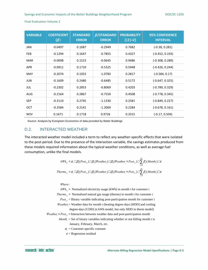
Savings and Economic Impacts of the Better Buildings Neighborhood Program DOE/EE-1203
Final Evaluation Volume 2
Alternate Billing Regression Model Specifications | Page D-5
VARIABLE COEFFICIENT
(𝜷)
STANDARD
ERROR
𝜷/STANDARD
ERROR
PROBABILITY
[|Z|>Z]
95% CONFIDENCE
INTERVAL
JAN -0.0497 0.1687 -0.2949 0.7682 (-0.38, 0.281)
FEB -0.1294 0.1647 -0.7855 0.4327 (-0.452, 0.193)
MAR -0.0098 0.1523 -0.0645 0.9486 (-0.308, 0.289)
APR -0.0911 0.1710 -0.5325 0.5948 (-0.426, 0.244)
MAY -0.2074 0.1923 -1.0783 0.2817 (-0.584, 0.17)
JUN -0.1609 0.2480 -0.6485 0.5172 (-0.647, 0.325)
JUL -0.2302 0.2853 -0.8069 0.4203 (-0.789, 0.329)
AUG -0.2164 0.2867 -0.7550 0.4508 (-0.778, 0.345)
SEP -0.3110 0.2745 -1.1330 0.2581 (-0.849, 0.227)
OCT -0.2584 0.2141 -1.2069 0.2284 (-0.678, 0.161)
NOV 0.1671 0.1718 0.9726 0.3315 (-0.17, 0.504)
Source: Analysis by Evergreen Economics of data provided by Better Buildings
D.2. INTERACTED WEATHER
The interacted weather model included a term to reflect any weather-specific effects that were isolated
to the post-period. Due to the presence of the interaction variable, the savings estimates produced from
these models required information about the typical weather conditions, as well as average fuel
consumption, unlike the final models.
kWhi,t = ai + b1(Posti,t )+ b2 (Weathert )+ b3(Weathert ´Posti,t )+ b j (Montht )j=4
14
å +e
Thermsi,t = ai + b1(Posti,t )+ b2 (Weathert )+ b3(Weathert ´Posti,t )+ b j (Montht )j=4
14
å +e
Where :
kWhi,t = Normalized electricity usage (kWh) in month t for customer i
Thermsi,t = Normalized natural gas usage (therms) in month t for customer i
Posti,t = Binary variable indicating post-participation month for customer i
Weathert= Weather data for month t (heating degree-days [HDD] and cooling
degree-days [CDD] in kWh model, but only HDD in therm model)
Weathert ´Posti,t = Interaction between weather data and post-participation month
Montht = Set of binary variables indicating whether or not billing month t is
January, February, March, etc.
ai = Customer-specific constant
e = Regression residual
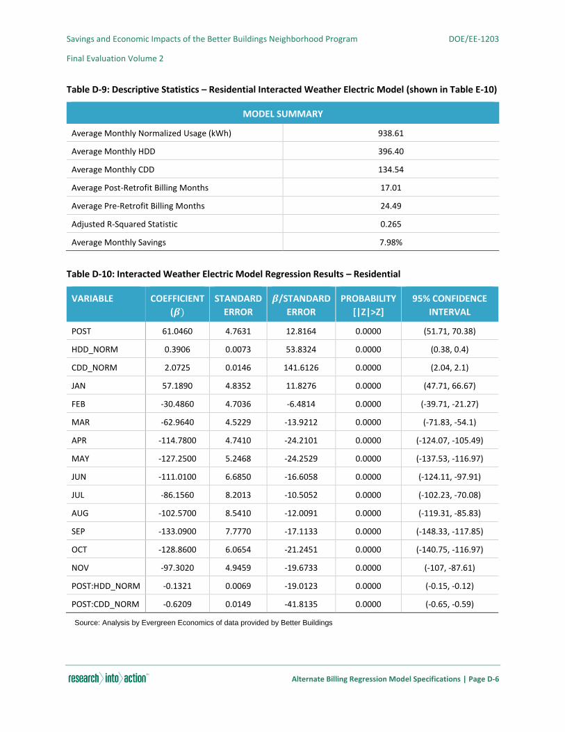
Savings and Economic Impacts of the Better Buildings Neighborhood Program DOE/EE-1203
Final Evaluation Volume 2
Alternate Billing Regression Model Specifications | Page D-6
Table D-9: Descriptive Statistics – Residential Interacted Weather Electric Model (shown in Table E-10)
MODEL SUMMARY
Average Monthly Normalized Usage (kWh) 938.61
Average Monthly HDD 396.40
Average Monthly CDD 134.54
Average Post-Retrofit Billing Months 17.01
Average Pre-Retrofit Billing Months 24.49
Adjusted R-Squared Statistic 0.265
Average Monthly Savings 7.98%
Table D-10: Interacted Weather Electric Model Regression Results – Residential
VARIABLE COEFFICIENT
(𝜷)
STANDARD
ERROR
𝜷/STANDARD
ERROR
PROBABILITY
[|Z|>Z]
95% CONFIDENCE
INTERVAL
POST 61.0460 4.7631 12.8164 0.0000 (51.71, 70.38)
HDD_NORM 0.3906 0.0073 53.8324 0.0000 (0.38, 0.4)
CDD_NORM 2.0725 0.0146 141.6126 0.0000 (2.04, 2.1)
JAN 57.1890 4.8352 11.8276 0.0000 (47.71, 66.67)
FEB -30.4860 4.7036 -6.4814 0.0000 (-39.71, -21.27)
MAR -62.9640 4.5229 -13.9212 0.0000 (-71.83, -54.1)
APR -114.7800 4.7410 -24.2101 0.0000 (-124.07, -105.49)
MAY -127.2500 5.2468 -24.2529 0.0000 (-137.53, -116.97)
JUN -111.0100 6.6850 -16.6058 0.0000 (-124.11, -97.91)
JUL -86.1560 8.2013 -10.5052 0.0000 (-102.23, -70.08)
AUG -102.5700 8.5410 -12.0091 0.0000 (-119.31, -85.83)
SEP -133.0900 7.7770 -17.1133 0.0000 (-148.33, -117.85)
OCT -128.8600 6.0654 -21.2451 0.0000 (-140.75, -116.97)
NOV -97.3020 4.9459 -19.6733 0.0000 (-107, -87.61)
POST:HDD_NORM -0.1321 0.0069 -19.0123 0.0000 (-0.15, -0.12)
POST:CDD_NORM -0.6209 0.0149 -41.8135 0.0000 (-0.65, -0.59)
Source: Analysis by Evergreen Economics of data provided by Better Buildings
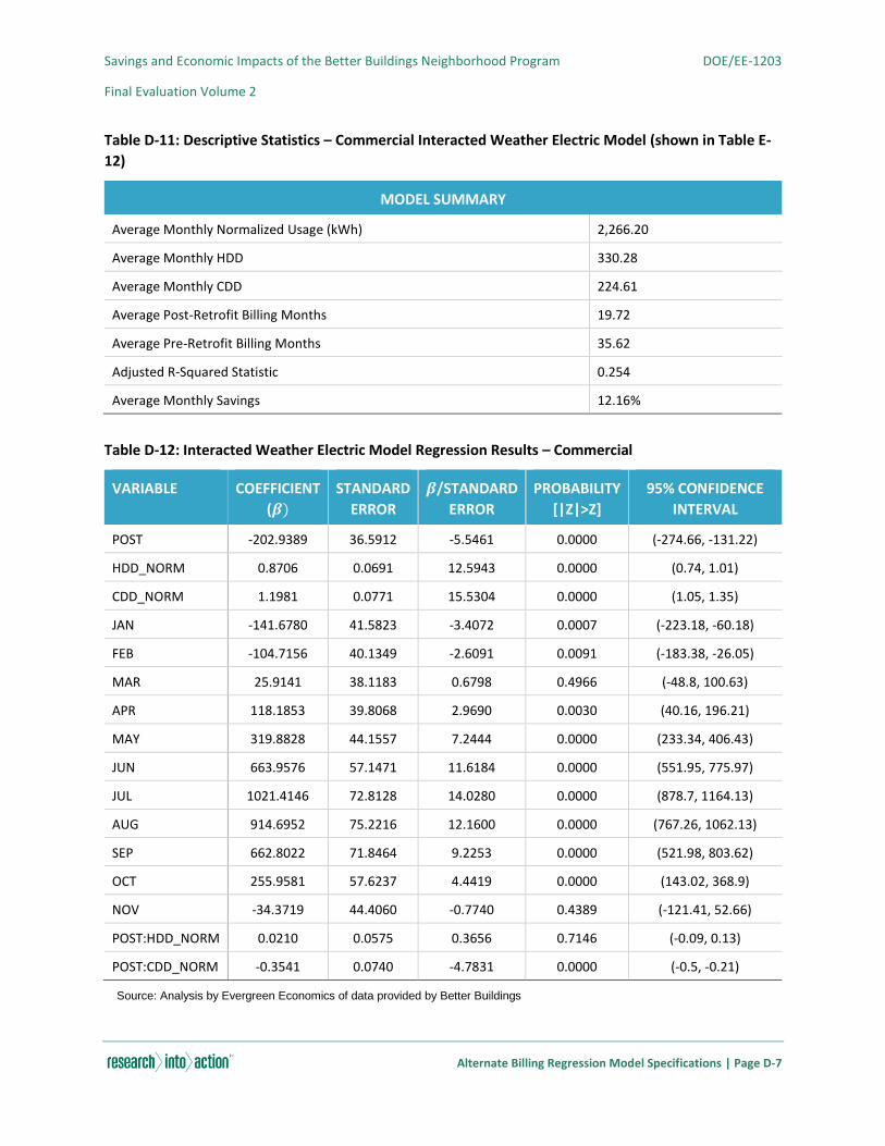
Savings and Economic Impacts of the Better Buildings Neighborhood Program DOE/EE-1203
Final Evaluation Volume 2
Alternate Billing Regression Model Specifications | Page D-7
Table D-11: Descriptive Statistics – Commercial Interacted Weather Electric Model (shown in Table E-
12)
MODEL SUMMARY
Average Monthly Normalized Usage (kWh) 2,266.20
Average Monthly HDD 330.28
Average Monthly CDD 224.61
Average Post-Retrofit Billing Months 19.72
Average Pre-Retrofit Billing Months 35.62
Adjusted R-Squared Statistic 0.254
Average Monthly Savings 12.16%
Table D-12: Interacted Weather Electric Model Regression Results – Commercial
VARIABLE COEFFICIENT
(𝜷)
STANDARD
ERROR
𝜷/STANDARD
ERROR
PROBABILITY
[|Z|>Z]
95% CONFIDENCE
INTERVAL
POST -202.9389 36.5912 -5.5461 0.0000 (-274.66, -131.22)
HDD_NORM 0.8706 0.0691 12.5943 0.0000 (0.74, 1.01)
CDD_NORM 1.1981 0.0771 15.5304 0.0000 (1.05, 1.35)
JAN -141.6780 41.5823 -3.4072 0.0007 (-223.18, -60.18)
FEB -104.7156 40.1349 -2.6091 0.0091 (-183.38, -26.05)
MAR 25.9141 38.1183 0.6798 0.4966 (-48.8, 100.63)
APR 118.1853 39.8068 2.9690 0.0030 (40.16, 196.21)
MAY 319.8828 44.1557 7.2444 0.0000 (233.34, 406.43)
JUN 663.9576 57.1471 11.6184 0.0000 (551.95, 775.97)
JUL 1021.4146 72.8128 14.0280 0.0000 (878.7, 1164.13)
AUG 914.6952 75.2216 12.1600 0.0000 (767.26, 1062.13)
SEP 662.8022 71.8464 9.2253 0.0000 (521.98, 803.62)
OCT 255.9581 57.6237 4.4419 0.0000 (143.02, 368.9)
NOV -34.3719 44.4060 -0.7740 0.4389 (-121.41, 52.66)
POST:HDD_NORM 0.0210 0.0575 0.3656 0.7146 (-0.09, 0.13)
POST:CDD_NORM -0.3541 0.0740 -4.7831 0.0000 (-0.5, -0.21)
Source: Analysis by Evergreen Economics of data provided by Better Buildings
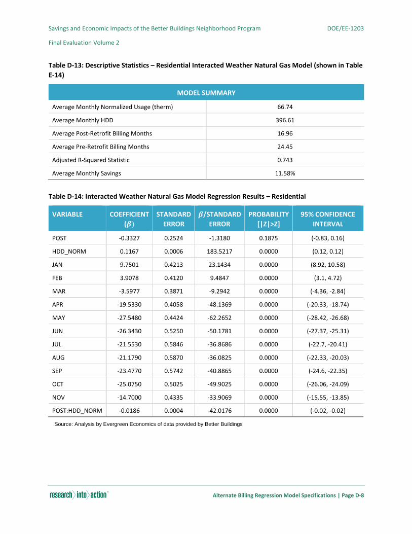
Savings and Economic Impacts of the Better Buildings Neighborhood Program DOE/EE-1203
Final Evaluation Volume 2
Alternate Billing Regression Model Specifications | Page D-8
Table D-13: Descriptive Statistics – Residential Interacted Weather Natural Gas Model (shown in Table
E-14)
MODEL SUMMARY
Average Monthly Normalized Usage (therm) 66.74
Average Monthly HDD 396.61
Average Post-Retrofit Billing Months 16.96
Average Pre-Retrofit Billing Months 24.45
Adjusted R-Squared Statistic 0.743
Average Monthly Savings 11.58%
Table D-14: Interacted Weather Natural Gas Model Regression Results – Residential
VARIABLE COEFFICIENT
(𝜷)
STANDARD
ERROR
𝜷/STANDARD
ERROR
PROBABILITY
[|Z|>Z]
95% CONFIDENCE
INTERVAL
POST -0.3327 0.2524 -1.3180 0.1875 (-0.83, 0.16)
HDD_NORM 0.1167 0.0006 183.5217 0.0000 (0.12, 0.12)
JAN 9.7501 0.4213 23.1434 0.0000 (8.92, 10.58)
FEB 3.9078 0.4120 9.4847 0.0000 (3.1, 4.72)
MAR -3.5977 0.3871 -9.2942 0.0000 (-4.36, -2.84)
APR -19.5330 0.4058 -48.1369 0.0000 (-20.33, -18.74)
MAY -27.5480 0.4424 -62.2652 0.0000 (-28.42, -26.68)
JUN -26.3430 0.5250 -50.1781 0.0000 (-27.37, -25.31)
JUL -21.5530 0.5846 -36.8686 0.0000 (-22.7, -20.41)
AUG -21.1790 0.5870 -36.0825 0.0000 (-22.33, -20.03)
SEP -23.4770 0.5742 -40.8865 0.0000 (-24.6, -22.35)
OCT -25.0750 0.5025 -49.9025 0.0000 (-26.06, -24.09)
NOV -14.7000 0.4335 -33.9069 0.0000 (-15.55, -13.85)
POST:HDD_NORM -0.0186 0.0004 -42.0176 0.0000 (-0.02, -0.02)
Source: Analysis by Evergreen Economics of data provided by Better Buildings
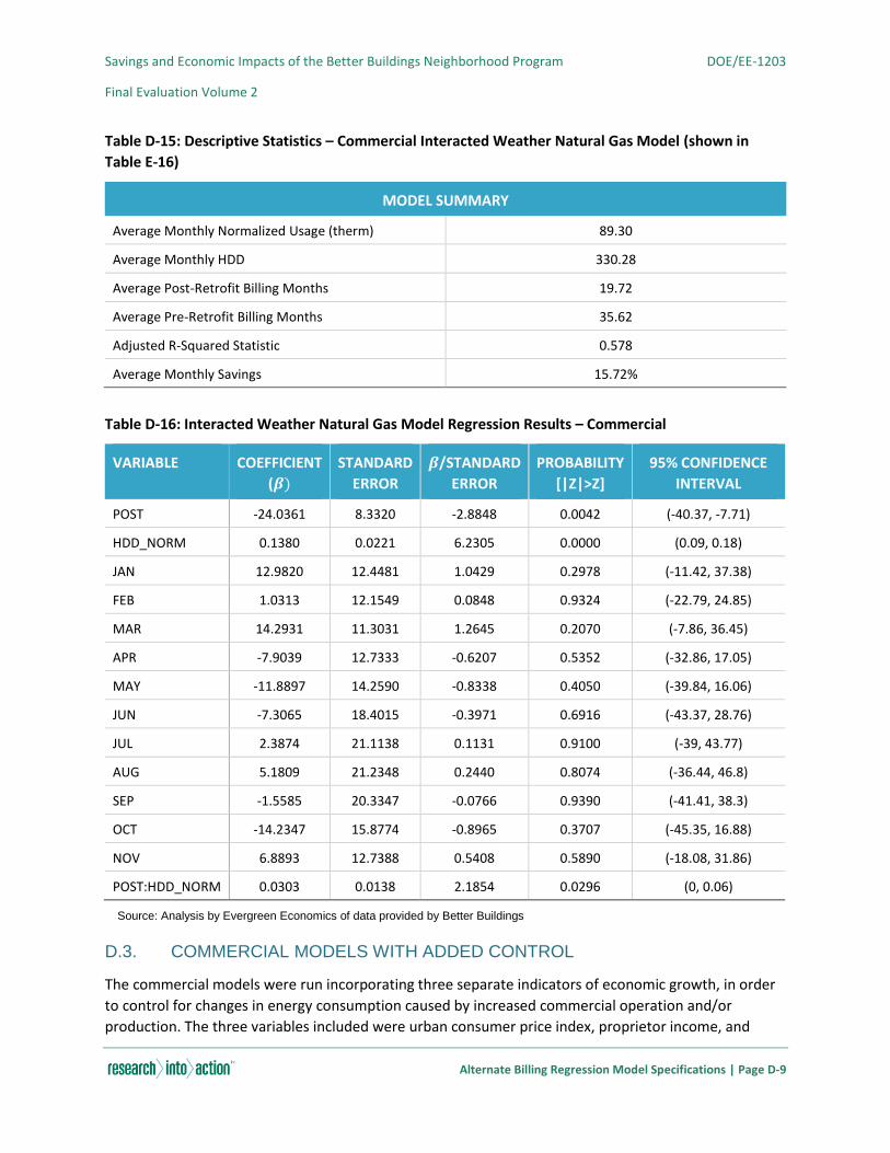
Savings and Economic Impacts of the Better Buildings Neighborhood Program DOE/EE-1203
Final Evaluation Volume 2
Alternate Billing Regression Model Specifications | Page D-9
Table D-15: Descriptive Statistics – Commercial Interacted Weather Natural Gas Model (shown in
Table E-16)
MODEL SUMMARY
Average Monthly Normalized Usage (therm) 89.30
Average Monthly HDD 330.28
Average Post-Retrofit Billing Months 19.72
Average Pre-Retrofit Billing Months 35.62
Adjusted R-Squared Statistic 0.578
Average Monthly Savings 15.72%
Table D-16: Interacted Weather Natural Gas Model Regression Results – Commercial
VARIABLE COEFFICIENT
(𝜷)
STANDARD
ERROR
𝜷/STANDARD
ERROR
PROBABILITY
[|Z|>Z]
95% CONFIDENCE
INTERVAL
POST -24.0361 8.3320 -2.8848 0.0042 (-40.37, -7.71)
HDD_NORM 0.1380 0.0221 6.2305 0.0000 (0.09, 0.18)
JAN 12.9820 12.4481 1.0429 0.2978 (-11.42, 37.38)
FEB 1.0313 12.1549 0.0848 0.9324 (-22.79, 24.85)
MAR 14.2931 11.3031 1.2645 0.2070 (-7.86, 36.45)
APR -7.9039 12.7333 -0.6207 0.5352 (-32.86, 17.05)
MAY -11.8897 14.2590 -0.8338 0.4050 (-39.84, 16.06)
JUN -7.3065 18.4015 -0.3971 0.6916 (-43.37, 28.76)
JUL 2.3874 21.1138 0.1131 0.9100 (-39, 43.77)
AUG 5.1809 21.2348 0.2440 0.8074 (-36.44, 46.8)
SEP -1.5585 20.3347 -0.0766 0.9390 (-41.41, 38.3)
OCT -14.2347 15.8774 -0.8965 0.3707 (-45.35, 16.88)
NOV 6.8893 12.7388 0.5408 0.5890 (-18.08, 31.86)
POST:HDD_NORM 0.0303 0.0138 2.1854 0.0296 (0, 0.06)
Source: Analysis by Evergreen Economics of data provided by Better Buildings
D.3. COMMERCIAL MODELS WITH ADDED CONTROL
The commercial models were run incorporating three separate indicators of economic growth, in order
to control for changes in energy consumption caused by increased commercial operation and/or
production. The three variables included were urban consumer price index, proprietor income, and
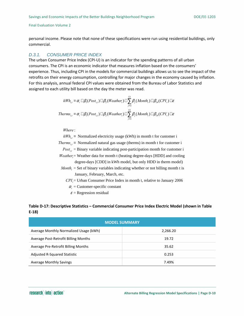
Savings and Economic Impacts of the Better Buildings Neighborhood Program DOE/EE-1203
Final Evaluation Volume 2
Alternate Billing Regression Model Specifications | Page D-10
personal income. Please note that none of these specifications were run using residential buildings, only
commercial.
D.3.1. CONSUMER PRICE INDEX The urban Consumer Price Index (CPI-U) is an indicator for the spending patterns of all urban
consumers. The CPI is an economic indicator that measures inflation based on the consumers’
experience. Thus, including CPI in the models for commercial buildings allows us to see the impact of the
retrofits on their energy consumption, controlling for major changes in the economy caused by inflation.
For this analysis, annual federal CPI values were obtained from the Bureau of Labor Statistics and
assigned to each utility bill based on the day the meter was read.
Table D-17: Descriptive Statistics – Commercial Consumer Price Index Electric Model (shown in Table
E-18)
MODEL SUMMARY
Average Monthly Normalized Usage (kWh) 2,266.20
Average Post-Retrofit Billing Months 19.72
Average Pre-Retrofit Billing Months 35.62
Adjusted R-Squared Statistic 0.253
Average Monthly Savings 7.49%
kWhi,t = ai + b1(Posti,t )+ b2 (Weathert )+ b j (Montht )j=3
13
å + b14(CPIt )+e
Thermsi,t = ai + b1(Posti,t )+ b2 (Weathert )+ b j (Montht )j=3
13
å + b14(CPIt )+e
Where :
kWhi,t = Normalized electricity usage (kWh) in month t for customer i
Thermsi,t = Normalized natural gas usage (therms) in month t for customer i
Posti,t = Binary variable indicating post-participation month for customer i
Weathert= Weather data for month t (heating degree-days [HDD] and cooling
degree-days [CDD] in kWh model, but only HDD in therm model)
Montht = Set of binary variables indicating whether or not billing month t is
January, February, March, etc.
CPIt= Urban Consumer Price Index in month t, relative to January 2006
ai = Customer-specific constant
e = Regression residual
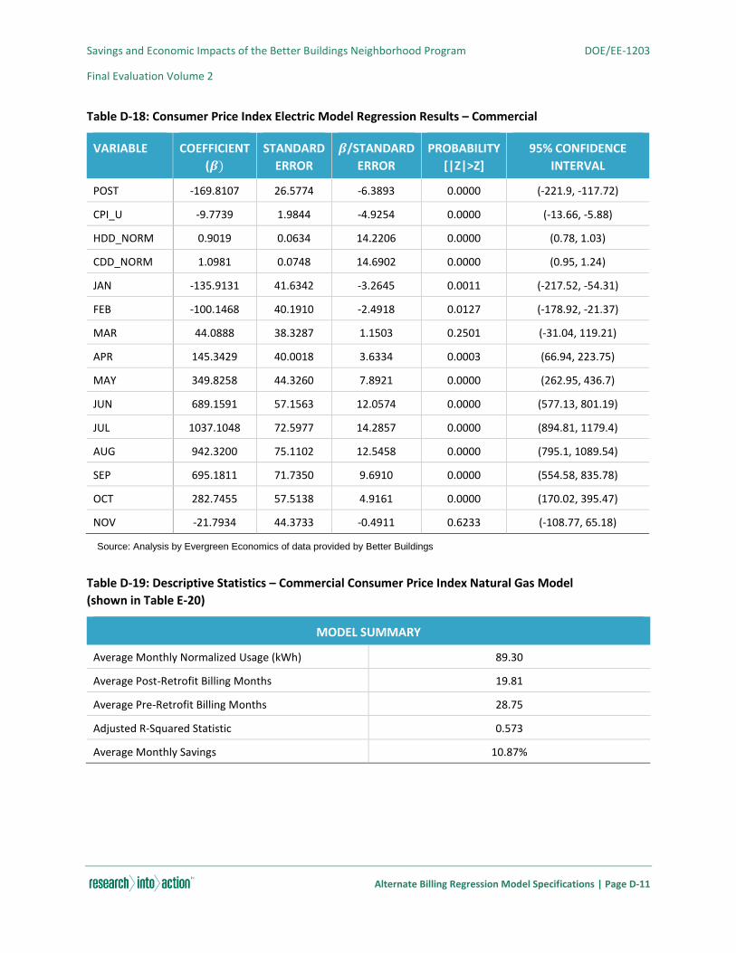
Savings and Economic Impacts of the Better Buildings Neighborhood Program DOE/EE-1203
Final Evaluation Volume 2
Alternate Billing Regression Model Specifications | Page D-11
Table D-18: Consumer Price Index Electric Model Regression Results – Commercial
VARIABLE COEFFICIENT
(𝜷)
STANDARD
ERROR
𝜷/STANDARD
ERROR
PROBABILITY
[|Z|>Z]
95% CONFIDENCE
INTERVAL
POST -169.8107 26.5774 -6.3893 0.0000 (-221.9, -117.72)
CPI_U -9.7739 1.9844 -4.9254 0.0000 (-13.66, -5.88)
HDD_NORM 0.9019 0.0634 14.2206 0.0000 (0.78, 1.03)
CDD_NORM 1.0981 0.0748 14.6902 0.0000 (0.95, 1.24)
JAN -135.9131 41.6342 -3.2645 0.0011 (-217.52, -54.31)
FEB -100.1468 40.1910 -2.4918 0.0127 (-178.92, -21.37)
MAR 44.0888 38.3287 1.1503 0.2501 (-31.04, 119.21)
APR 145.3429 40.0018 3.6334 0.0003 (66.94, 223.75)
MAY 349.8258 44.3260 7.8921 0.0000 (262.95, 436.7)
JUN 689.1591 57.1563 12.0574 0.0000 (577.13, 801.19)
JUL 1037.1048 72.5977 14.2857 0.0000 (894.81, 1179.4)
AUG 942.3200 75.1102 12.5458 0.0000 (795.1, 1089.54)
SEP 695.1811 71.7350 9.6910 0.0000 (554.58, 835.78)
OCT 282.7455 57.5138 4.9161 0.0000 (170.02, 395.47)
NOV -21.7934 44.3733 -0.4911 0.6233 (-108.77, 65.18)
Source: Analysis by Evergreen Economics of data provided by Better Buildings
Table D-19: Descriptive Statistics – Commercial Consumer Price Index Natural Gas Model
(shown in Table E-20)
MODEL SUMMARY
Average Monthly Normalized Usage (kWh) 89.30
Average Post-Retrofit Billing Months 19.81
Average Pre-Retrofit Billing Months 28.75
Adjusted R-Squared Statistic 0.573
Average Monthly Savings 10.87%
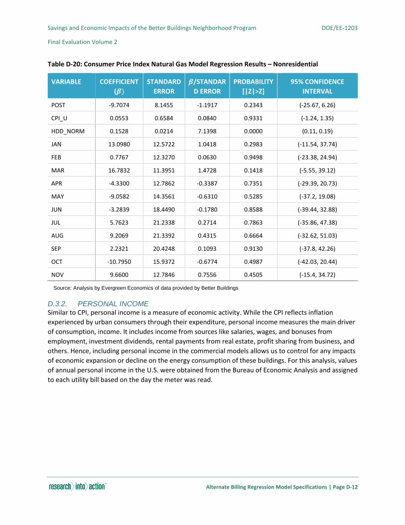
Savings and Economic Impacts of the Better Buildings Neighborhood Program DOE/EE-1203
Final Evaluation Volume 2
Alternate Billing Regression Model Specifications | Page D-12
Table D-20: Consumer Price Index Natural Gas Model Regression Results – Nonresidential
VARIABLE COEFFICIENT
(𝜷)
STANDARD
ERROR
𝜷/STANDAR
D ERROR
PROBABILITY
[|Z|>Z]
95% CONFIDENCE
INTERVAL
POST -9.7074 8.1455 -1.1917 0.2343 (-25.67, 6.26)
CPI_U 0.0553 0.6584 0.0840 0.9331 (-1.24, 1.35)
HDD_NORM 0.1528 0.0214 7.1398 0.0000 (0.11, 0.19)
JAN 13.0980 12.5722 1.0418 0.2983 (-11.54, 37.74)
FEB 0.7767 12.3270 0.0630 0.9498 (-23.38, 24.94)
MAR 16.7832 11.3951 1.4728 0.1418 (-5.55, 39.12)
APR -4.3300 12.7862 -0.3387 0.7351 (-29.39, 20.73)
MAY -9.0582 14.3561 -0.6310 0.5285 (-37.2, 19.08)
JUN -3.2839 18.4490 -0.1780 0.8588 (-39.44, 32.88)
JUL 5.7623 21.2338 0.2714 0.7863 (-35.86, 47.38)
AUG 9.2069 21.3392 0.4315 0.6664 (-32.62, 51.03)
SEP 2.2321 20.4248 0.1093 0.9130 (-37.8, 42.26)
OCT -10.7950 15.9372 -0.6774 0.4987 (-42.03, 20.44)
NOV 9.6600 12.7846 0.7556 0.4505 (-15.4, 34.72)
Source: Analysis by Evergreen Economics of data provided by Better Buildings
D.3.2. PERSONAL INCOME Similar to CPI, personal income is a measure of economic activity. While the CPI reflects inflation
experienced by urban consumers through their expenditure, personal income measures the main driver
of consumption, income. It includes income from sources like salaries, wages, and bonuses from
employment, investment dividends, rental payments from real estate, profit sharing from business, and
others. Hence, including personal income in the commercial models allows us to control for any impacts
of economic expansion or decline on the energy consumption of these buildings. For this analysis, values
of annual personal income in the U.S. were obtained from the Bureau of Economic Analysis and assigned
to each utility bill based on the day the meter was read.
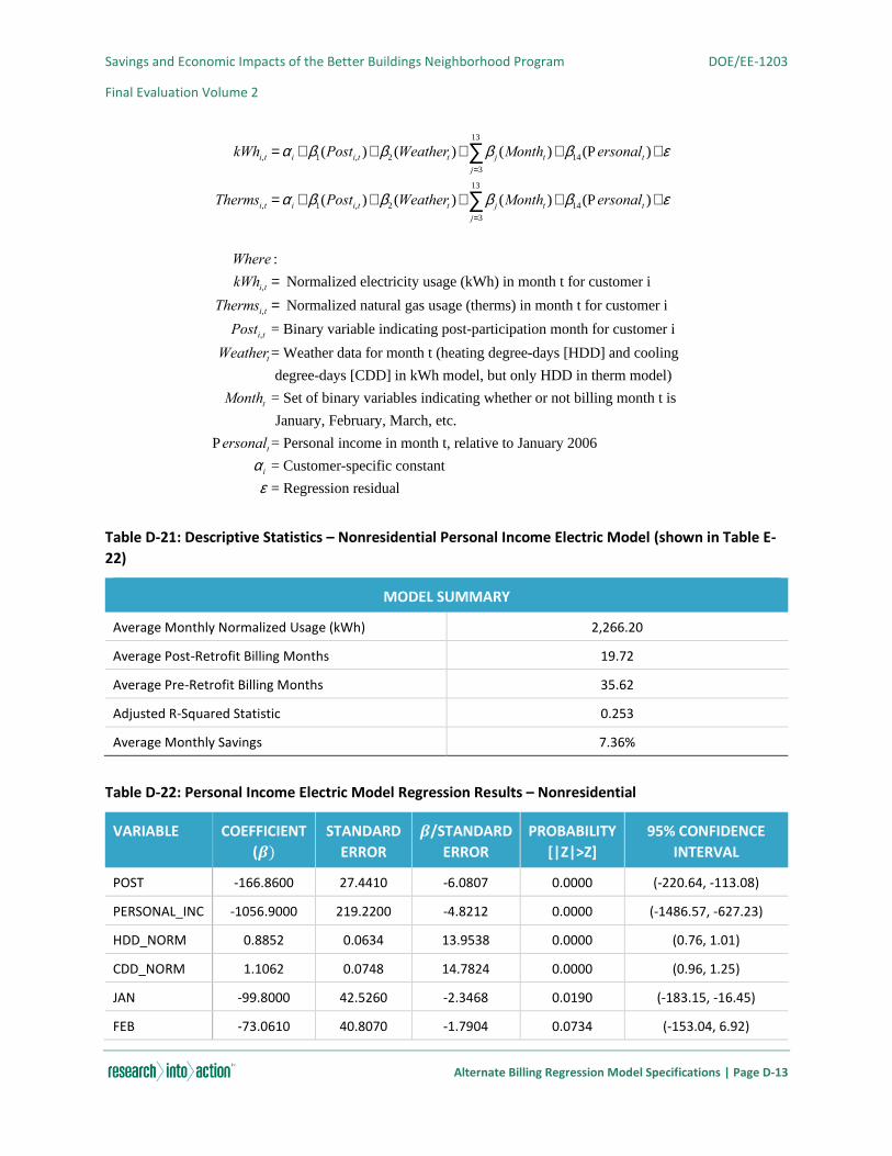
Savings and Economic Impacts of the Better Buildings Neighborhood Program DOE/EE-1203
Final Evaluation Volume 2
Alternate Billing Regression Model Specifications | Page D-13
Table D-21: Descriptive Statistics – Nonresidential Personal Income Electric Model (shown in Table E-
22)
MODEL SUMMARY
Average Monthly Normalized Usage (kWh) 2,266.20
Average Post-Retrofit Billing Months 19.72
Average Pre-Retrofit Billing Months 35.62
Adjusted R-Squared Statistic 0.253
Average Monthly Savings 7.36%
Table D-22: Personal Income Electric Model Regression Results – Nonresidential
VARIABLE COEFFICIENT
(𝜷)
STANDARD
ERROR
𝜷/STANDARD
ERROR
PROBABILITY
[|Z|>Z]
95% CONFIDENCE
INTERVAL
POST -166.8600 27.4410 -6.0807 0.0000 (-220.64, -113.08)
PERSONAL_INC -1056.9000 219.2200 -4.8212 0.0000 (-1486.57, -627.23)
HDD_NORM 0.8852 0.0634 13.9538 0.0000 (0.76, 1.01)
CDD_NORM 1.1062 0.0748 14.7824 0.0000 (0.96, 1.25)
JAN -99.8000 42.5260 -2.3468 0.0190 (-183.15, -16.45)
FEB -73.0610 40.8070 -1.7904 0.0734 (-153.04, 6.92)
kWhi,t = ai + b1(Posti,t )+ b2 (Weathert )+ b j (Montht )j=3
13
å + b14(Personalt )+e
Thermsi,t = ai + b1(Posti,t )+ b2 (Weathert )+ b j (Montht )j=3
13
å + b14(Personalt )+e
Where :
kWhi,t = Normalized electricity usage (kWh) in month t for customer i
Thermsi,t = Normalized natural gas usage (therms) in month t for customer i
Posti,t = Binary variable indicating post-participation month for customer i
Weathert= Weather data for month t (heating degree-days [HDD] and cooling
degree-days [CDD] in kWh model, but only HDD in therm model)
Montht = Set of binary variables indicating whether or not billing month t is
January, February, March, etc.
Personalt= Personal income in month t, relative to January 2006
ai = Customer-specific constant
e = Regression residual
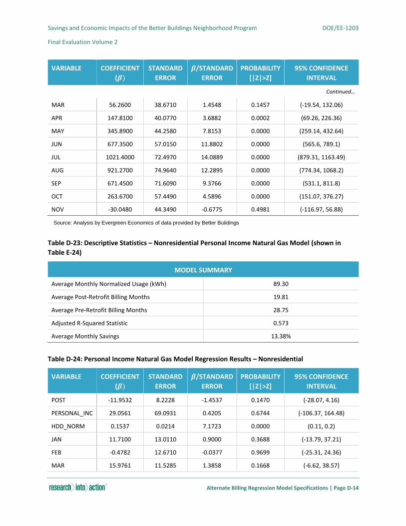
Savings and Economic Impacts of the Better Buildings Neighborhood Program DOE/EE-1203
Final Evaluation Volume 2
Alternate Billing Regression Model Specifications | Page D-14
VARIABLE COEFFICIENT
(𝜷)
STANDARD
ERROR
𝜷/STANDARD
ERROR
PROBABILITY
[|Z|>Z]
95% CONFIDENCE
INTERVAL
Continued…
MAR 56.2600 38.6710 1.4548 0.1457 (-19.54, 132.06)
APR 147.8100 40.0770 3.6882 0.0002 (69.26, 226.36)
MAY 345.8900 44.2580 7.8153 0.0000 (259.14, 432.64)
JUN 677.3500 57.0150 11.8802 0.0000 (565.6, 789.1)
JUL 1021.4000 72.4970 14.0889 0.0000 (879.31, 1163.49)
AUG 921.2700 74.9640 12.2895 0.0000 (774.34, 1068.2)
SEP 671.4500 71.6090 9.3766 0.0000 (531.1, 811.8)
OCT 263.6700 57.4490 4.5896 0.0000 (151.07, 376.27)
NOV -30.0480 44.3490 -0.6775 0.4981 (-116.97, 56.88)
Source: Analysis by Evergreen Economics of data provided by Better Buildings
Table D-23: Descriptive Statistics – Nonresidential Personal Income Natural Gas Model (shown in
Table E-24)
MODEL SUMMARY
Average Monthly Normalized Usage (kWh) 89.30
Average Post-Retrofit Billing Months 19.81
Average Pre-Retrofit Billing Months 28.75
Adjusted R-Squared Statistic 0.573
Average Monthly Savings 13.38%
Table D-24: Personal Income Natural Gas Model Regression Results – Nonresidential
VARIABLE COEFFICIENT
(𝜷)
STANDARD
ERROR
𝜷/STANDARD
ERROR
PROBABILITY
[|Z|>Z]
95% CONFIDENCE
INTERVAL
POST -11.9532 8.2228 -1.4537 0.1470 (-28.07, 4.16)
PERSONAL_INC 29.0561 69.0931 0.4205 0.6744 (-106.37, 164.48)
HDD_NORM 0.1537 0.0214 7.1723 0.0000 (0.11, 0.2)
JAN 11.7100 13.0110 0.9000 0.3688 (-13.79, 37.21)
FEB -0.4782 12.6710 -0.0377 0.9699 (-25.31, 24.36)
MAR 15.9761 11.5285 1.3858 0.1668 (-6.62, 38.57)
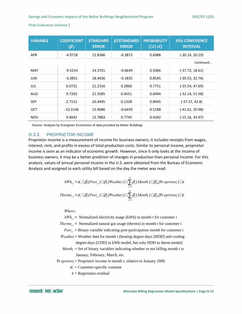
Savings and Economic Impacts of the Better Buildings Neighborhood Program DOE/EE-1203
Final Evaluation Volume 2
Alternate Billing Regression Model Specifications | Page D-15
VARIABLE COEFFICIENT
(𝜷)
STANDARD
ERROR
𝜷/STANDARD
ERROR
PROBABILITY
[|Z|>Z]
95% CONFIDENCE
INTERVAL
APR -4.9718 12.8386 -0.3873 0.6988 (-30.14, 20.19)
Continued…
MAY -9.5554 14.3701 -0.6649 0.5066 (-37.72, 18.61)
JUN -3.3851 18.4436 -0.1835 0.8545 (-39.53, 32.76)
JUL 6.0721 21.2316 0.2860 0.7751 (-35.54, 47.69)
AUG 9.7203 21.3585 0.4551 0.6494 (-32.14, 51.58)
SEP 2.7152 20.4495 0.1328 0.8945 (-37.37, 42.8)
OCT -10.3146 15.9686 -0.6459 0.5188 (-41.61, 20.98)
NOV 9.9042 12.7883 0.7745 0.4392 (-15.16, 34.97)
Source: Analysis by Evergreen Economics of data provided by Better Buildings
D.3.3. PROPRIETOR INCOME Proprietor income is a measurement of income for business owners; it includes receipts from wages,
interest, rent, and profits in excess of total production costs. Similar to personal income, proprietor
income is seen as an indicator of economic growth. However, since it only looks at the income of
business owners, it may be a better predictor of changes in production than personal income. For this
analysis, values of annual personal income in the U.S. were obtained from the Bureau of Economic
Analysis and assigned to each utility bill based on the day the meter was read.
kWhi,t = ai + b1(Posti,t )+ b2 (Weathert )+ b j (Montht )j=3
13
å + b14 (Proprietort )+e
Thermsi,t = ai + b1(Posti,t )+ b2 (Weathert )+ b j (Montht )j=3
13
å + b14 (Proprietort )+e
Where :
kWhi,t = Normalized electricity usage (kWh) in month t for customer i
Thermsi,t = Normalized natural gas usage (therms) in month t for customer i
Posti,t = Binary variable indicating post-participation month for customer i
Weathert= Weather data for month t (heating degree-days [HDD] and cooling
degree-days [CDD] in kWh model, but only HDD in therm model)
Montht = Set of binary variables indicating whether or not billing month t is
January, February, March, etc.
Proprietort= Proprietor income in month t, relative to January 2006
ai = Customer-specific constant
e = Regression residual

Savings and Economic Impacts of the Better Buildings Neighborhood Program DOE/EE-1203
Final Evaluation Volume 2
Alternate Billing Regression Model Specifications | Page D-16
Table D-25: Descriptive Statistics – Nonresidential Proprietor Income Electric Model (shown in Table E-
26)
MODEL SUMMARY
Average Monthly Normalized Usage (kWh) 2,266.20
Average Post-Retrofit Billing Months 19.72
Average Pre-Retrofit Billing Months 35.62
Adjusted R-Squared Statistic 0.253
Average Monthly Savings 6.90%
Table D-26: Proprietor Income Electric Model Regression Results – Nonresidential
VARIABLE COEFFICIENT
(𝜷)
STANDARD
ERROR
𝜷/STANDARD
ERROR
PROBABILITY
[|Z|>Z]
95% CONFIDENCE
INTERVAL
POST -156.4711 26.7801 -5.8428 0.0000 (-208.96, -103.98)
PROPRIETOR_INC -681.9722 124.2760 -5.4876 0.0000 (-925.55, -438.39)
HDD_NORM 0.8947 0.0634 14.1150 0.0000 (0.77, 1.02)
CDD_NORM 1.0981 0.0747 14.6955 0.0000 (0.95, 1.24)
JAN -95.5065 42.4578 -2.2494 0.0245 (-178.72, -12.29)
FEB -69.6183 40.7517 -1.7084 0.0876 (-149.49, 10.26)
MAR 60.3659 38.6569 1.5616 0.1184 (-15.4, 136.13)
APR 154.5103 40.1467 3.8486 0.0001 (75.82, 233.2)
MAY 353.7633 44.3408 7.9783 0.0000 (266.86, 440.67)
JUN 687.6823 57.0858 12.0465 0.0000 (575.79, 799.57)
JUL 1034.3042 72.5354 14.2593 0.0000 (892.13, 1176.47)
AUG 934.3938 74.9939 12.4596 0.0000 (787.41, 1081.38)
SEP 682.5489 71.6037 9.5323 0.0000 (542.21, 822.89)
OCT 270.1250 57.4256 4.7039 0.0000 (157.57, 382.68)
NOV -26.9958 44.3380 -0.6089 0.5426 (-113.9, 59.91)
Source: Analysis by Evergreen Economics of data provided by Better Buildings
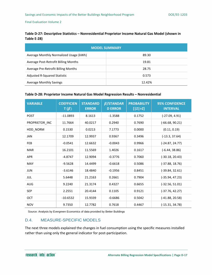
Savings and Economic Impacts of the Better Buildings Neighborhood Program DOE/EE-1203
Final Evaluation Volume 2
Alternate Billing Regression Model Specifications | Page D-17
Table D-27: Descriptive Statistics – Nonresidential Proprietor Income Natural Gas Model (shown in
Table E-28)
MODEL SUMMARY
Average Monthly Normalized Usage (kWh) 89.30
Average Post-Retrofit Billing Months 19.81
Average Pre-Retrofit Billing Months 28.75
Adjusted R-Squared Statistic 0.573
Average Monthly Savings 12.42%
Table D-28: Proprietor Income Natural Gas Model Regression Results – Nonresidential
VARIABLE COEFFICIEN
T (𝜷)
STANDARD
ERROR
𝜷/STANDAR
D ERROR
PROBABILITY
[|Z|>Z]
95% CONFIDENCE
INTERVAL
POST -11.0893 8.1613 -1.3588 0.1752 (-27.09, 4.91)
PROPRIETOR_INC 11.7664 40.0217 0.2940 0.7690 (-66.68, 90.21)
HDD_NORM 0.1530 0.0213 7.1773 0.0000 (0.11, 0.19)
JAN 12.1709 12.9937 0.9367 0.3496 (-13.3, 37.64)
FEB -0.0541 12.6632 -0.0043 0.9966 (-24.87, 24.77)
MAR 16.2101 11.5569 1.4026 0.1617 (-6.44, 38.86)
APR -4.8747 12.9094 -0.3776 0.7060 (-30.18, 20.43)
MAY -9.5628 14.4499 -0.6618 0.5086 (-37.88, 18.76)
JUN -3.6146 18.4840 -0.1956 0.8451 (-39.84, 32.61)
JUL 5.6448 21.2163 0.2661 0.7904 (-35.94, 47.23)
AUG 9.2240 21.3174 0.4327 0.6655 (-32.56, 51.01)
SEP 2.2551 20.4144 0.1105 0.9121 (-37.76, 42.27)
OCT -10.6532 15.9339 -0.6686 0.5042 (-41.88, 20.58)
NOV 9.7350 12.7782 0.7618 0.4467 (-15.31, 34.78)
Source: Analysis by Evergreen Economics of data provided by Better Buildings
D.4. MEASURE-SPECIFIC MODELS
The next three models explained the changes in fuel consumption using the specific measures installed
rather than using only the general indicator for post-participation.

Savings and Economic Impacts of the Better Buildings Neighborhood Program DOE/EE-1203
Final Evaluation Volume 2
Alternate Billing Regression Model Specifications | Page D-18
D.4.1. NUMBER OF DIFFERENT TYPES OF MEASURES INSTALLED The simplest of these is the measure count model, which used the sum of the binary installed measure
flags from the tracking data as an indication of the number of different types of measures installed. The
measure count was interacted with the indicator for the post-period so that the model would estimate
the impact of each additional measure on fuel consumption in the post-period.
Table D-29: Descriptive Statistics – Residential Measure Count Electric Model (shown in Table E-30)
MODEL SUMMARY
Average Monthly Normalized Usage (kWh) 938.61
Average Number of Measure Types Installed 3.61
Average Post-Retrofit Billing Months 17.01
Average Pre-Retrofit Billing Months 24.49
Adjusted R-Squared Statistic 0.261
Average Monthly Savings per Measure Type Installed 1.61%
Average Monthly Savings 5.82%
Table D-30: Measure Count Electric Model Regression Results – Residential
VARIABLE COEFFICIENT
(𝜷)
STANDARD
ERROR
𝜷/STANDARD
ERROR
PROBABILITY
[|Z|>Z]
95% CONFIDENCE
INTERVAL
MEAS_COUNT -15.1280 0.4499 -33.6260 0.0000 (-16.01, -14.246)
kWhi,t =ai + b1(MeasCounti ´Posti,t )+ b2(Weathert )+ b j (Montht )j=3
13
å +e
Thermsi,t =ai + b1(MeasCounti ´Posti,t )+ b2(Weathert )+ b j (Montht )j=3
13
å +e
Where :
kWhi,t= Normalized electricity usage (kWh) in month t for customer i
Thermsi,t= Normalized natural gas usage (therms) in month t for customer i
MeasCounti = Number of different types of measures installed for customer i, from tracking data
Posti,t= Binary variable indicating post-participation month for customer i
Weathert= Weather data for month t (heating degree-days [HDD] and cooling
degree-days [CDD] in kWh model, but only HDD in therm model)
Montht = Set of binary variables indicating whether or not billing month t is
January, February, March, etc.
ai = Customer-specific constant
e = Regression residual
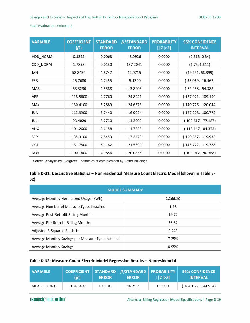
Savings and Economic Impacts of the Better Buildings Neighborhood Program DOE/EE-1203
Final Evaluation Volume 2
Alternate Billing Regression Model Specifications | Page D-19
VARIABLE COEFFICIENT
(𝜷)
STANDARD
ERROR
𝜷/STANDARD
ERROR
PROBABILITY
[|Z|>Z]
95% CONFIDENCE
INTERVAL
HDD_NORM 0.3265 0.0068 48.0926 0.0000 (0.313, 0.34)
CDD_NORM 1.7853 0.0130 137.2041 0.0000 (1.76, 1.811)
JAN 58.8450 4.8747 12.0715 0.0000 (49.291, 68.399)
FEB -25.7680 4.7455 -5.4300 0.0000 (-35.069, -16.467)
MAR -63.3230 4.5588 -13.8903 0.0000 (-72.258, -54.388)
APR -118.5600 4.7760 -24.8241 0.0000 (-127.921, -109.199)
MAY -130.4100 5.2889 -24.6573 0.0000 (-140.776, -120.044)
JUN -113.9900 6.7440 -16.9024 0.0000 (-127.208, -100.772)
JUL -93.4020 8.2730 -11.2900 0.0000 (-109.617, -77.187)
AUG -101.2600 8.6158 -11.7528 0.0000 (-118.147, -84.373)
SEP -135.3100 7.8453 -17.2473 0.0000 (-150.687, -119.933)
OCT -131.7800 6.1182 -21.5390 0.0000 (-143.772, -119.788)
NOV -100.1400 4.9856 -20.0858 0.0000 (-109.912, -90.368)
Source: Analysis by Evergreen Economics of data provided by Better Buildings
Table D-31: Descriptive Statistics – Nonresidential Measure Count Electric Model (shown in Table E-
32)
MODEL SUMMARY
Average Monthly Normalized Usage (kWh) 2,266.20
Average Number of Measure Types Installed 1.23
Average Post-Retrofit Billing Months 19.72
Average Pre-Retrofit Billing Months 35.62
Adjusted R-Squared Statistic 0.249
Average Monthly Savings per Measure Type Installed 7.25%
Average Monthly Savings 8.95%
Table D-32: Measure Count Electric Model Regression Results – Nonresidential
VARIABLE COEFFICIENT
(𝜷)
STANDARD
ERROR
𝜷/STANDARD
ERROR
PROBABILITY
[|Z|>Z]
95% CONFIDENCE
INTERVAL
MEAS_COUNT -164.3497 10.1101 -16.2559 0.0000 (-184.166, -144.534)

Savings and Economic Impacts of the Better Buildings Neighborhood Program DOE/EE-1203
Final Evaluation Volume 2
Alternate Billing Regression Model Specifications | Page D-20
VARIABLE COEFFICIENT
(𝜷)
STANDARD
ERROR
𝜷/STANDARD
ERROR
PROBABILITY
[|Z|>Z]
95% CONFIDENCE
INTERVAL
HDD_NORM 0.9292 0.0634 14.6565 0.0000 (0.805, 1.053)
CDD_NORM 1.0457 0.0747 14.0026 0.0000 (0.899, 1.192)
JAN -151.7037 41.6885 -3.6390 0.0003 (-233.413, -69.994)
FEB -114.7536 40.2416 -2.8516 0.0044 (-193.627, -35.88)
MAR 22.2342 38.2282 0.5816 0.5608 (-52.693, 97.161)
APR 126.0935 39.8291 3.1659 0.0016 (48.028, 204.158)
MAY 335.8474 44.1602 7.6052 0.0000 (249.294, 422.401)
JUN 686.8816 57.0240 12.0455 0.0000 (575.114, 798.649)
JUL 1047.7013 72.5421 14.4427 0.0000 (905.519, 1189.884)
AUG 950.8669 75.0071 12.6770 0.0000 (803.853, 1097.881)
SEP 705.4004 71.6322 9.8475 0.0000 (565.001, 845.8)
OCT 294.1645 57.4659 5.1189 0.0000 (181.531, 406.798)
NOV -15.9467 44.4169 -0.3590 0.7196 (-103.004, 71.11)
Source: Analysis by Evergreen Economics of data provided by Better Buildings
Table D-33: Descriptive Statistics – Residential Measure Count Natural Gas Model (shown in Table E-
34)
MODEL SUMMARY
Average Monthly Normalized Usage (therm) 66.74
Average Number of Measure Types Installed 3.55
Average Post-Retrofit Billing Months 17.70
Average Pre-Retrofit Billing Months 30.22
Adjusted R-Squared Statistic 0.740
Average Monthly Savings per Measure Type Installed 3.35%
Average Monthly Savings 11.90%
Table D-34: Measure Count Natural Gas Model Regression Results – Residential
VARIABLE COEFFICIENT
(𝜷)
STANDARD
ERROR
𝜷/STANDARD
ERROR
PROBABILITY
[|Z|>Z]
95% CONFIDENCE
INTERVAL
MEAS_COUNT -2.2351 0.0425 -52.6327 0.0000 (-2.318, -2.152)
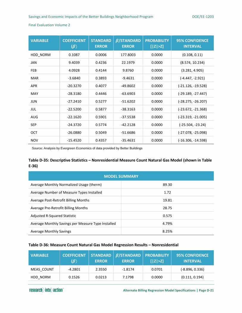
Savings and Economic Impacts of the Better Buildings Neighborhood Program DOE/EE-1203
Final Evaluation Volume 2
Alternate Billing Regression Model Specifications | Page D-21
VARIABLE COEFFICIENT
(𝜷)
STANDARD
ERROR
𝜷/STANDARD
ERROR
PROBABILITY
[|Z|>Z]
95% CONFIDENCE
INTERVAL
HDD_NORM 0.1087 0.0006 177.8003 0.0000 (0.108, 0.11)
JAN 9.4039 0.4236 22.1979 0.0000 (8.574, 10.234)
FEB 4.0928 0.4144 9.8760 0.0000 (3.281, 4.905)
MAR -3.6840 0.3893 -9.4631 0.0000 (-4.447, -2.921)
APR -20.3270 0.4077 -49.8602 0.0000 (-21.126, -19.528)
MAY -28.3180 0.4446 -63.6903 0.0000 (-29.189, -27.447)
JUN -27.2410 0.5277 -51.6202 0.0000 (-28.275, -26.207)
JUL -22.5200 0.5877 -38.3163 0.0000 (-23.672, -21.368)
AUG -22.1620 0.5901 -37.5538 0.0000 (-23.319, -21.005)
SEP -24.3720 0.5774 -42.2128 0.0000 (-25.504, -23.24)
OCT -26.0880 0.5049 -51.6686 0.0000 (-27.078, -25.098)
NOV -15.4520 0.4357 -35.4631 0.0000 (-16.306, -14.598)
Source: Analysis by Evergreen Economics of data provided by Better Buildings
Table D-35: Descriptive Statistics – Nonresidential Measure Count Natural Gas Model (shown in Table
E-36)
MODEL SUMMARY
Average Monthly Normalized Usage (therm) 89.30
Average Number of Measure Types Installed 1.72
Average Post-Retrofit Billing Months 19.81
Average Pre-Retrofit Billing Months 28.75
Adjusted R-Squared Statistic 0.575
Average Monthly Savings per Measure Type Installed 4.79%
Average Monthly Savings 8.25%
Table D-36: Measure Count Natural Gas Model Regression Results – Nonresidential
VARIABLE COEFFICIENT
(𝜷)
STANDARD
ERROR
𝜷/STANDARD
ERROR
PROBABILITY
[|Z|>Z]
95% CONFIDENCE
INTERVAL
MEAS_COUNT -4.2801 2.3550 -1.8174 0.0701 (-8.896, 0.336)
HDD_NORM 0.1526 0.0213 7.1798 0.0000 (0.111, 0.194)
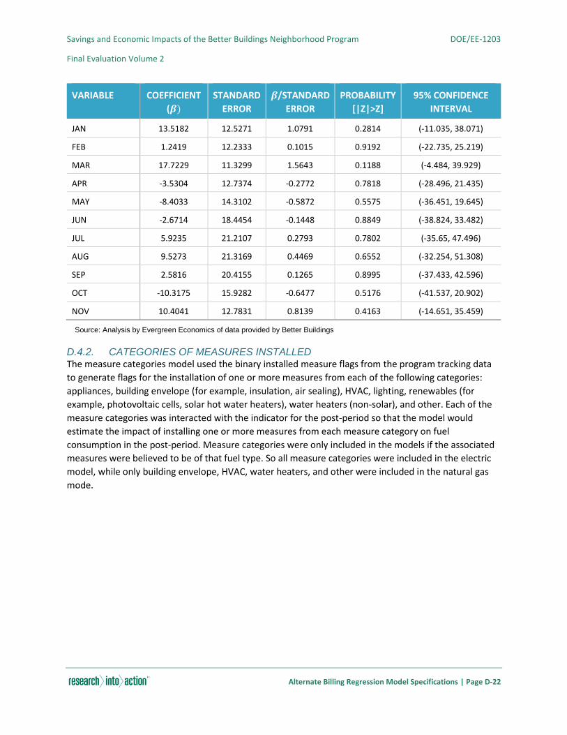
Savings and Economic Impacts of the Better Buildings Neighborhood Program DOE/EE-1203
Final Evaluation Volume 2
Alternate Billing Regression Model Specifications | Page D-22
VARIABLE COEFFICIENT
(𝜷)
STANDARD
ERROR
𝜷/STANDARD
ERROR
PROBABILITY
[|Z|>Z]
95% CONFIDENCE
INTERVAL
JAN 13.5182 12.5271 1.0791 0.2814 (-11.035, 38.071)
FEB 1.2419 12.2333 0.1015 0.9192 (-22.735, 25.219)
MAR 17.7229 11.3299 1.5643 0.1188 (-4.484, 39.929)
APR -3.5304 12.7374 -0.2772 0.7818 (-28.496, 21.435)
MAY -8.4033 14.3102 -0.5872 0.5575 (-36.451, 19.645)
JUN -2.6714 18.4454 -0.1448 0.8849 (-38.824, 33.482)
JUL 5.9235 21.2107 0.2793 0.7802 (-35.65, 47.496)
AUG 9.5273 21.3169 0.4469 0.6552 (-32.254, 51.308)
SEP 2.5816 20.4155 0.1265 0.8995 (-37.433, 42.596)
OCT -10.3175 15.9282 -0.6477 0.5176 (-41.537, 20.902)
NOV 10.4041 12.7831 0.8139 0.4163 (-14.651, 35.459)
Source: Analysis by Evergreen Economics of data provided by Better Buildings
D.4.2. CATEGORIES OF MEASURES INSTALLED The measure categories model used the binary installed measure flags from the program tracking data
to generate flags for the installation of one or more measures from each of the following categories:
appliances, building envelope (for example, insulation, air sealing), HVAC, lighting, renewables (for
example, photovoltaic cells, solar hot water heaters), water heaters (non-solar), and other. Each of the
measure categories was interacted with the indicator for the post-period so that the model would
estimate the impact of installing one or more measures from each measure category on fuel
consumption in the post-period. Measure categories were only included in the models if the associated
measures were believed to be of that fuel type. So all measure categories were included in the electric
model, while only building envelope, HVAC, water heaters, and other were included in the natural gas
mode.
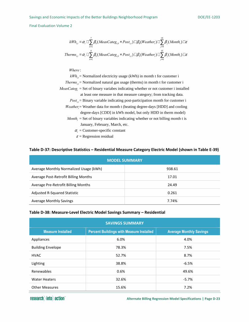
Savings and Economic Impacts of the Better Buildings Neighborhood Program DOE/EE-1203
Final Evaluation Volume 2
Alternate Billing Regression Model Specifications | Page D-23
Table D-37: Descriptive Statistics – Residential Measure Category Electric Model (shown in Table E-39)
MODEL SUMMARY
Average Monthly Normalized Usage (kWh) 938.61
Average Post-Retrofit Billing Months 17.01
Average Pre-Retrofit Billing Months 24.49
Adjusted R-Squared Statistic 0.261
Average Monthly Savings 7.74%
Table D-38: Measure-Level Electric Model Savings Summary – Residential
SAVINGS SUMMARY
Measure Installed Percent Buildings with Measure Installed Average Monthly Savings
Appliances 6.0% 4.0%
Building Envelope 78.3% 7.5%
HVAC 52.7% 8.7%
Lighting 38.8% -6.5%
Renewables 0.6% 49.6%
Water Heaters 32.6% -5.7%
Other Measures 15.6% 7.2%
kWhi,t =ai + bk (MeasCategi,k ´Posti,t )k=1
7
å + b8(Weathert )+ b j (Montht )j=9
19
å +e
Thermsi,t =ai + bk (MeasCategi,k ´Posti,t )k=1
4
å + b5(Weathert )+ b j (Montht )j=6
16
å +e
Where :
kWhi,t= Normalized electricity usage (kWh) in month t for customer i
Thermsi,t= Normalized natural gas usage (therms) in month t for customer i
MeasCategi = Set of binary variabes indicating whether or not customer i installed
at least one measure in that measure category; from tracking data.
Posti,t= Binary variable indicating post-participation month for customer i
Weathert= Weather data for month t (heating degree-days [HDD] and cooling
degree-days [CDD] in kWh model, but only HDD in therm model)
Montht = Set of binary variables indicating whether or not billing month t is
January, February, March, etc.
ai = Customer-specific constant
e = Regression residual

Savings and Economic Impacts of the Better Buildings Neighborhood Program DOE/EE-1203
Final Evaluation Volume 2
Alternate Billing Regression Model Specifications | Page D-24
Table D-39: Measure Categories Electric Model Regression Results – Residential
VARIABLE COEFFICIENT
(𝜷)
STANDARD
ERROR
𝜷/STANDARD
ERROR
PROBABILITY
[|Z|>Z]
95% CONFIDENCE
INTERVAL
MEAS_APP -37.6490 7.5789 -4.9676 0.0000 (-52.5, -22.79)
MEAS_ENVL -70.6830 2.8139 -25.1192 0.0000 (-76.2, -65.17)
MEAS_HVAC -81.3750 3.2715 -24.8739 0.0000 (-87.79, -74.96)
MEAS_LIGHT 61.3440 5.0726 12.0932 0.0000 (51.4, 71.29)
MEAS_RENEW -465.4300 22.4230 -20.7568 0.0000 (-509.38, -421.48)
MEAS_WH 53.5100 5.2243 10.2425 0.0000 (43.27, 63.75)
MEAS_OTHER -67.4760 5.5072 -12.2523 0.0000 (-78.27, -56.68)
HDD_NORM 0.3237 0.0068 47.9210 0.0000 (0.31, 0.34)
CDD_NORM 1.8033 0.0130 139.1113 0.0000 (1.78, 1.83)
JAN 59.8190 4.8510 12.3313 0.0000 (50.31, 69.33)
FEB -27.6110 4.7228 -5.8463 0.0000 (-36.87, -18.35)
MAR -64.7340 4.5374 -14.2668 0.0000 (-73.63, -55.84)
APR -120.8000 4.7534 -25.4134 0.0000 (-130.12, -111.48)
MAY -134.0100 5.2643 -25.4564 0.0000 (-144.33, -123.69)
JUN -119.1100 6.7119 -17.7461 0.0000 (-132.27, -105.95)
JUL -102.3500 8.2375 -12.4249 0.0000 (-118.5, -86.2)
AUG -111.6300 8.5806 -13.0096 0.0000 (-128.45, -94.81)
SEP -143.6800 7.8124 -18.3913 0.0000 (-158.99, -128.37)
OCT -135.7800 6.0891 -22.2989 0.0000 (-147.71, -123.85)
NOV -101.8600 4.9622 -20.5272 0.0000 (-111.59, -92.13)
Source: Analysis by Evergreen Economics of data provided by Better Buildings
Table D-40: Descriptive Statistics – Nonresidential Measure Category Electric Model (shown in Table E-
42)
MODEL SUMMARY
Average Monthly Normalized Usage (kWh) 2,266.20
Average Post-Retrofit Billing Months 19.72
Average Pre-Retrofit Billing Months 35.62
Adjusted R-Squared Statistic 0.252
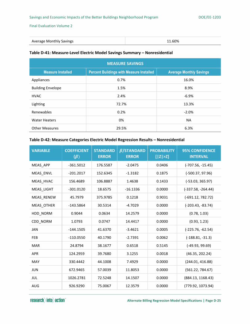
Savings and Economic Impacts of the Better Buildings Neighborhood Program DOE/EE-1203
Final Evaluation Volume 2
Alternate Billing Regression Model Specifications | Page D-25
Average Monthly Savings 11.60%
Table D-41: Measure-Level Electric Model Savings Summary – Nonresidential
MEASURE SAVINGS
Measure Installed Percent Buildings with Measure Installed Average Monthly Savings
Appliances 0.7% 16.0%
Building Envelope 1.5% 8.9%
HVAC 2.4% -6.9%
Lighting 72.7% 13.3%
Renewables 0.2% -2.0%
Water Heaters 0% NA
Other Measures 29.5% 6.3%
Table D-42: Measure Categories Electric Model Regression Results – Nonresidential
VARIABLE COEFFICIENT
(𝜷)
STANDARD
ERROR
𝜷/STANDARD
ERROR
PROBABILITY
[|Z|>Z]
95% CONFIDENCE
INTERVAL
MEAS_APP -361.5012 176.5587 -2.0475 0.0406 (-707.56, -15.45)
MEAS_ENVL -201.2017 152.6345 -1.3182 0.1875 (-500.37, 97.96)
MEAS_HVAC 156.4689 106.8887 1.4638 0.1433 (-53.03, 365.97)
MEAS_LIGHT -301.0120 18.6575 -16.1336 0.0000 (-337.58, -264.44)
MEAS_RENEW 45.7979 375.9785 0.1218 0.9031 (-691.12, 782.72)
MEAS_OTHER -143.5864 30.5314 -4.7029 0.0000 (-203.43, -83.74)
HDD_NORM 0.9044 0.0634 14.2579 0.0000 (0.78, 1.03)
CDD_NORM 1.0793 0.0747 14.4417 0.0000 (0.93, 1.23)
JAN -144.1505 41.6370 -3.4621 0.0005 (-225.76, -62.54)
FEB -110.0550 40.1790 -2.7391 0.0062 (-188.81, -31.3)
MAR 24.8794 38.1677 0.6518 0.5145 (-49.93, 99.69)
APR 124.2959 39.7680 3.1255 0.0018 (46.35, 202.24)
MAY 330.4442 44.1008 7.4929 0.0000 (244.01, 416.88)
JUN 672.9465 57.0039 11.8053 0.0000 (561.22, 784.67)
JUL 1026.2781 72.5248 14.1507 0.0000 (884.13, 1168.43)
AUG 926.9290 75.0067 12.3579 0.0000 (779.92, 1073.94)
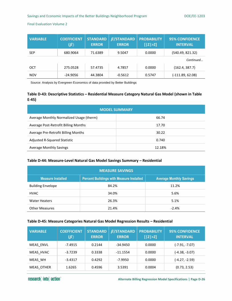
Savings and Economic Impacts of the Better Buildings Neighborhood Program DOE/EE-1203
Final Evaluation Volume 2
Alternate Billing Regression Model Specifications | Page D-26
VARIABLE COEFFICIENT
(𝜷)
STANDARD
ERROR
𝜷/STANDARD
ERROR
PROBABILITY
[|Z|>Z]
95% CONFIDENCE
INTERVAL
SEP 680.9064 71.6389 9.5047 0.0000 (540.49, 821.32)
Continued…
OCT 275.0528 57.4735 4.7857 0.0000 (162.4, 387.7)
NOV -24.9056 44.3804 -0.5612 0.5747 (-111.89, 62.08)
Source: Analysis by Evergreen Economics of data provided by Better Buildings
Table D-43: Descriptive Statistics – Residential Measure Category Natural Gas Model (shown in Table
E-45)
MODEL SUMMARY
Average Monthly Normalized Usage (therm) 66.74
Average Post-Retrofit Billing Months 17.70
Average Pre-Retrofit Billing Months 30.22
Adjusted R-Squared Statistic 0.740
Average Monthly Savings 12.18%
Table D-44: Measure-Level Natural Gas Model Savings Summary – Residential
MEASURE SAVINGS
Measure Installed Percent Buildings with Measure Installed Average Monthly Savings
Building Envelope 84.2% 11.2%
HVAC 34.0% 5.6%
Water Heaters 26.3% 5.1%
Other Measures 21.4% -2.4%
Table D-45: Measure Categories Natural Gas Model Regression Results – Residential
VARIABLE COEFFICIENT
(𝜷)
STANDARD
ERROR
𝜷/STANDARD
ERROR
PROBABILITY
[|Z|>Z]
95% CONFIDENCE
INTERVAL
MEAS_ENVL -7.4915 0.2144 -34.9450 0.0000 (-7.91, -7.07)
MEAS_HVAC -3.7239 0.3338 -11.1554 0.0000 (-4.38, -3.07)
MEAS_WH -3.4317 0.4292 -7.9950 0.0000 (-4.27, -2.59)
MEAS_OTHER 1.6265 0.4596 3.5391 0.0004 (0.73, 2.53)
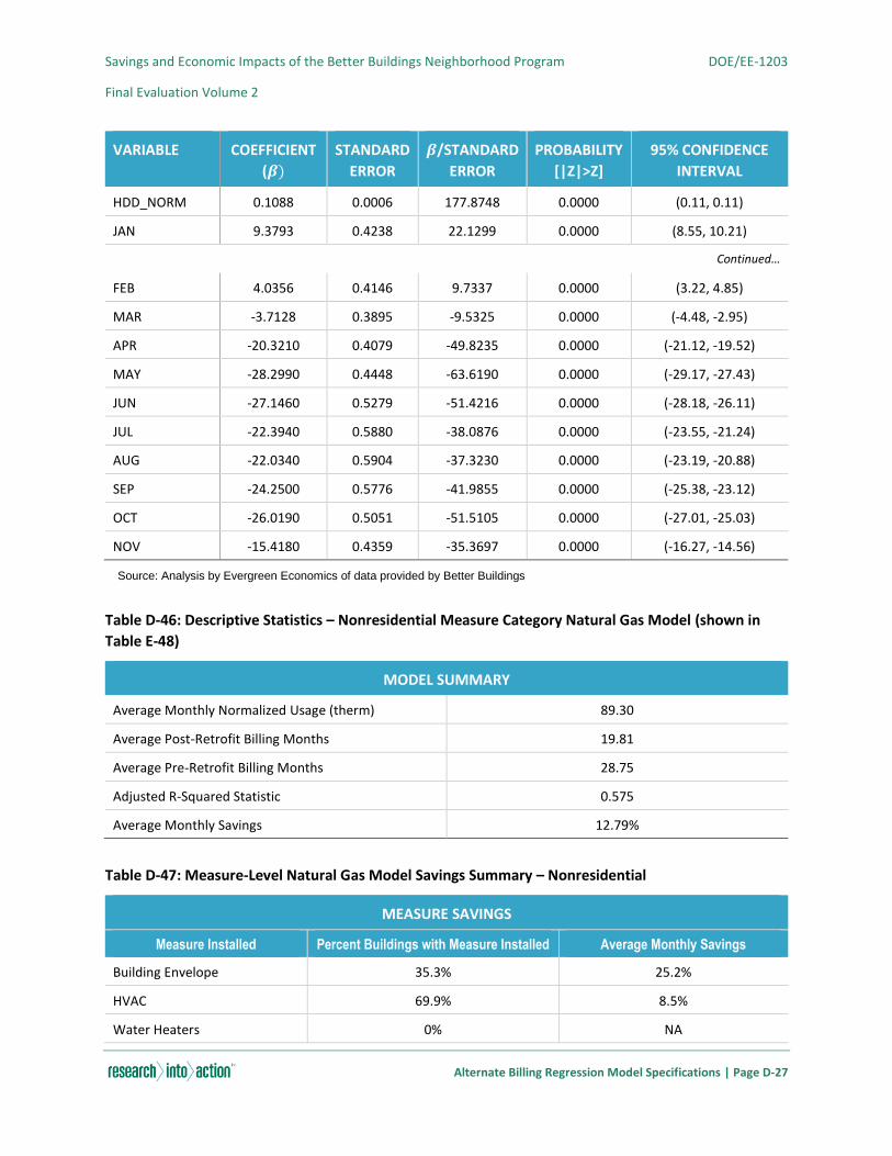
Savings and Economic Impacts of the Better Buildings Neighborhood Program DOE/EE-1203
Final Evaluation Volume 2
Alternate Billing Regression Model Specifications | Page D-27
VARIABLE COEFFICIENT
(𝜷)
STANDARD
ERROR
𝜷/STANDARD
ERROR
PROBABILITY
[|Z|>Z]
95% CONFIDENCE
INTERVAL
HDD_NORM 0.1088 0.0006 177.8748 0.0000 (0.11, 0.11)
JAN 9.3793 0.4238 22.1299 0.0000 (8.55, 10.21)
Continued…
FEB 4.0356 0.4146 9.7337 0.0000 (3.22, 4.85)
MAR -3.7128 0.3895 -9.5325 0.0000 (-4.48, -2.95)
APR -20.3210 0.4079 -49.8235 0.0000 (-21.12, -19.52)
MAY -28.2990 0.4448 -63.6190 0.0000 (-29.17, -27.43)
JUN -27.1460 0.5279 -51.4216 0.0000 (-28.18, -26.11)
JUL -22.3940 0.5880 -38.0876 0.0000 (-23.55, -21.24)
AUG -22.0340 0.5904 -37.3230 0.0000 (-23.19, -20.88)
SEP -24.2500 0.5776 -41.9855 0.0000 (-25.38, -23.12)
OCT -26.0190 0.5051 -51.5105 0.0000 (-27.01, -25.03)
NOV -15.4180 0.4359 -35.3697 0.0000 (-16.27, -14.56)
Source: Analysis by Evergreen Economics of data provided by Better Buildings
Table D-46: Descriptive Statistics – Nonresidential Measure Category Natural Gas Model (shown in
Table E-48)
MODEL SUMMARY
Average Monthly Normalized Usage (therm) 89.30
Average Post-Retrofit Billing Months 19.81
Average Pre-Retrofit Billing Months 28.75
Adjusted R-Squared Statistic 0.575
Average Monthly Savings 12.79%
Table D-47: Measure-Level Natural Gas Model Savings Summary – Nonresidential
MEASURE SAVINGS
Measure Installed Percent Buildings with Measure Installed Average Monthly Savings
Building Envelope 35.3% 25.2%
HVAC 69.9% 8.5%
Water Heaters 0% NA

Savings and Economic Impacts of the Better Buildings Neighborhood Program DOE/EE-1203
Final Evaluation Volume 2
Alternate Billing Regression Model Specifications | Page D-28
Other Measures 42.1% -4.8%
Table D-48: Measure Categories Natural Gas Model Regression Results – Nonresidential
VARIABLE COEFFICIENT
(𝜷)
STANDARD
ERROR
𝜷/STANDARD
ERROR
PROBABILITY
[|Z|>Z]
95% CONFIDENCE
INTERVAL
MEAS_ENVL -22.4674 10.4814 -2.1435 0.0328 (-43.01, -1.92)
MEAS_HVAC -7.5852 6.6747 -1.1364 0.2567 (-20.67, 5.5)
MEAS_OTHER 4.3197 9.5785 0.4510 0.6523 (-14.45, 23.09)
HDD_NORM 0.1504 0.0212 7.0917 0.0000 (0.11, 0.19)
JAN 13.2963 12.4856 1.0649 0.2877 (-11.18, 37.77)
FEB 1.4046 12.1934 0.1152 0.9084 (-22.49, 25.3)
MAR 16.8030 11.2966 1.4874 0.1379 (-5.34, 38.94)
APR -4.2922 12.6862 -0.3383 0.7353 (-29.16, 20.57)
MAY -9.3629 14.2635 -0.6564 0.5120 (-37.32, 18.59)
JUN -4.5726 18.4096 -0.2484 0.8040 (-40.66, 31.51)
JUL 3.3404 21.1443 0.1580 0.8746 (-38.1, 44.78)
AUG 7.0780 21.2512 0.3331 0.7393 (-34.57, 48.73)
SEP 0.2509 20.3519 0.0123 0.9902 (-39.64, 40.14)
OCT -11.9663 15.8855 -0.7533 0.4518 (-43.1, 19.17)
NOV 8.4781 12.7586 0.6645 0.5069 (-16.53, 33.48)
Source: Analysis by Evergreen Economics of data provided by Better Buildings
D.4.3. RETROFIT COMPREHENSIVENESS Similarly, the core and non-core points model expressed the change in consumption using a value
representing the comprehensiveness of the building retrofit. The core and non-core points were
assigned based on the binary installed measure flags in the program tracking data, according to a point
system similar to that used in the BBNP process evaluation.
For example, each project could receive a maximum of one core point for heating and one core point for
cooling. So a project that installed a heat pump would receive two core points (one for heating and one
for cooling), while a project that installed two heating measures (for example, new furnace and a high
efficiency wood stove) would only receive one core point (for heating).
Appliances and lighting controls are examples of measures that earned non-core points, because their
impact on overall energy consumption is not expected to be as significant as core measures like
insulation or photovoltaic cells. The maximum number of points across all grantees was 6 core and 6
non-core; the average project in the billing data has 2.2 core and 0.8 non-core points.
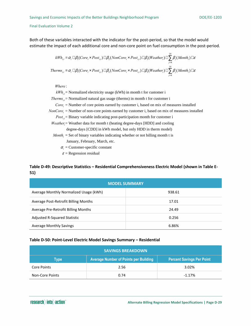
Savings and Economic Impacts of the Better Buildings Neighborhood Program DOE/EE-1203
Final Evaluation Volume 2
Alternate Billing Regression Model Specifications | Page D-29
Both of these variables interacted with the indicator for the post-period, so that the model would
estimate the impact of each additional core and non-core point on fuel consumption in the post-period.
Table D-49: Descriptive Statistics – Residential Comprehensiveness Electric Model (shown in Table E-
51)
MODEL SUMMARY
Average Monthly Normalized Usage (kWh) 938.61
Average Post-Retrofit Billing Months 17.01
Average Pre-Retrofit Billing Months 24.49
Adjusted R-Squared Statistic 0.256
Average Monthly Savings 6.86%
Table D-50: Point-Level Electric Model Savings Summary – Residential
SAVINGS BREAKDOWN
Type Average Number of Points per Building Percent Savings Per Point
Core Points 2.56 3.02%
Non-Core Points 0.74 -1.17%
kWhi,t =ai + b1(Corei ´Posti,t )+ b2 (NonCorei ´Posti,t )+ b3(Weathert )+ b j (Montht )j=4
14
å +e
Thermsi,t =ai + b1(Corei ´Posti,t )+ b2 (NonCorei ´Posti,t )+ b3(Weathert )+ b j (Montht )j=4
14
å +e
Where :
kWhi,t= Normalized electricity usage (kWh) in month t for customer i
Thermsi,t= Normalized natural gas usage (therms) in month t for customer i
Corei = Number of core points earned by customer i, based on mix of measures installed
NonCorei = Number of non-core points earned by customer i, based on mix of measures installed
Posti,t= Binary variable indicating post-participation month for customer i
Weathert= Weather data for month t (heating degree-days [HDD] and cooling
degree-days [CDD] in kWh model, but only HDD in therm model)
Montht = Set of binary variables indicating whether or not billing month t is
January, February, March, etc.
ai = Customer-specific constant
e = Regression residual
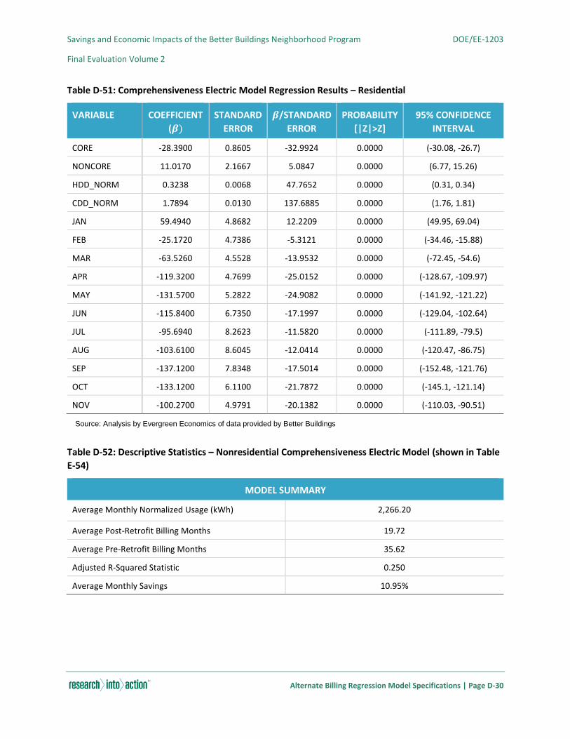
Savings and Economic Impacts of the Better Buildings Neighborhood Program DOE/EE-1203
Final Evaluation Volume 2
Alternate Billing Regression Model Specifications | Page D-30
Table D-51: Comprehensiveness Electric Model Regression Results – Residential
VARIABLE COEFFICIENT
(𝜷)
STANDARD
ERROR
𝜷/STANDARD
ERROR
PROBABILITY
[|Z|>Z]
95% CONFIDENCE
INTERVAL
CORE -28.3900 0.8605 -32.9924 0.0000 (-30.08, -26.7)
NONCORE 11.0170 2.1667 5.0847 0.0000 (6.77, 15.26)
HDD_NORM 0.3238 0.0068 47.7652 0.0000 (0.31, 0.34)
CDD_NORM 1.7894 0.0130 137.6885 0.0000 (1.76, 1.81)
JAN 59.4940 4.8682 12.2209 0.0000 (49.95, 69.04)
FEB -25.1720 4.7386 -5.3121 0.0000 (-34.46, -15.88)
MAR -63.5260 4.5528 -13.9532 0.0000 (-72.45, -54.6)
APR -119.3200 4.7699 -25.0152 0.0000 (-128.67, -109.97)
MAY -131.5700 5.2822 -24.9082 0.0000 (-141.92, -121.22)
JUN -115.8400 6.7350 -17.1997 0.0000 (-129.04, -102.64)
JUL -95.6940 8.2623 -11.5820 0.0000 (-111.89, -79.5)
AUG -103.6100 8.6045 -12.0414 0.0000 (-120.47, -86.75)
SEP -137.1200 7.8348 -17.5014 0.0000 (-152.48, -121.76)
OCT -133.1200 6.1100 -21.7872 0.0000 (-145.1, -121.14)
NOV -100.2700 4.9791 -20.1382 0.0000 (-110.03, -90.51)
Source: Analysis by Evergreen Economics of data provided by Better Buildings
Table D-52: Descriptive Statistics – Nonresidential Comprehensiveness Electric Model (shown in Table
E-54)
MODEL SUMMARY
Average Monthly Normalized Usage (kWh) 2,266.20
Average Post-Retrofit Billing Months 19.72
Average Pre-Retrofit Billing Months 35.62
Adjusted R-Squared Statistic 0.250
Average Monthly Savings 10.95%
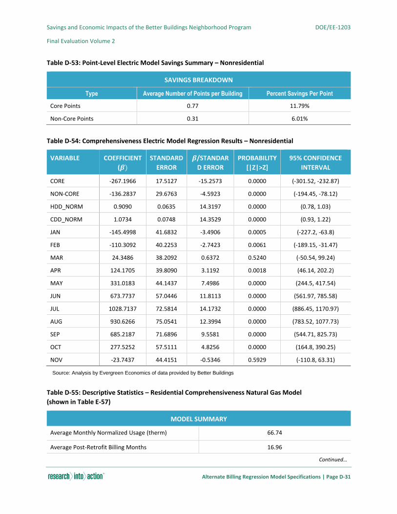
Savings and Economic Impacts of the Better Buildings Neighborhood Program DOE/EE-1203
Final Evaluation Volume 2
Alternate Billing Regression Model Specifications | Page D-31
Table D-53: Point-Level Electric Model Savings Summary – Nonresidential
SAVINGS BREAKDOWN
Type Average Number of Points per Building Percent Savings Per Point
Core Points 0.77 11.79%
Non-Core Points 0.31 6.01%
Table D-54: Comprehensiveness Electric Model Regression Results – Nonresidential
VARIABLE COEFFICIENT
(𝜷)
STANDARD
ERROR
𝜷/STANDAR
D ERROR
PROBABILITY
[|Z|>Z]
95% CONFIDENCE
INTERVAL
CORE -267.1966 17.5127 -15.2573 0.0000 (-301.52, -232.87)
NON-CORE -136.2837 29.6763 -4.5923 0.0000 (-194.45, -78.12)
HDD_NORM 0.9090 0.0635 14.3197 0.0000 (0.78, 1.03)
CDD_NORM 1.0734 0.0748 14.3529 0.0000 (0.93, 1.22)
JAN -145.4998 41.6832 -3.4906 0.0005 (-227.2, -63.8)
FEB -110.3092 40.2253 -2.7423 0.0061 (-189.15, -31.47)
MAR 24.3486 38.2092 0.6372 0.5240 (-50.54, 99.24)
APR 124.1705 39.8090 3.1192 0.0018 (46.14, 202.2)
MAY 331.0183 44.1437 7.4986 0.0000 (244.5, 417.54)
JUN 673.7737 57.0446 11.8113 0.0000 (561.97, 785.58)
JUL 1028.7137 72.5814 14.1732 0.0000 (886.45, 1170.97)
AUG 930.6266 75.0541 12.3994 0.0000 (783.52, 1077.73)
SEP 685.2187 71.6896 9.5581 0.0000 (544.71, 825.73)
OCT 277.5252 57.5111 4.8256 0.0000 (164.8, 390.25)
NOV -23.7437 44.4151 -0.5346 0.5929 (-110.8, 63.31)
Source: Analysis by Evergreen Economics of data provided by Better Buildings
Table D-55: Descriptive Statistics – Residential Comprehensiveness Natural Gas Model
(shown in Table E-57)
MODEL SUMMARY
Average Monthly Normalized Usage (therm) 66.74
Average Post-Retrofit Billing Months 16.96
Continued…
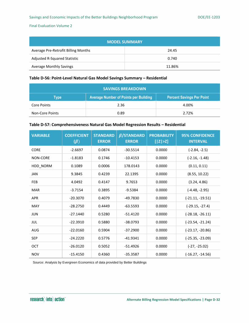
Savings and Economic Impacts of the Better Buildings Neighborhood Program DOE/EE-1203
Final Evaluation Volume 2
Alternate Billing Regression Model Specifications | Page D-32
MODEL SUMMARY
Average Pre-Retrofit Billing Months 24.45
Adjusted R-Squared Statistic 0.740
Average Monthly Savings 11.86%
Table D-56: Point-Level Natural Gas Model Savings Summary – Residential
SAVINGS BREAKDOWN
Type Average Number of Points per Building Percent Savings Per Point
Core Points 2.36 4.00%
Non-Core Points 0.89 2.72%
Table D-57: Comprehensiveness Natural Gas Model Regression Results – Residential
VARIABLE COEFFICIENT
(𝜷)
STANDARD
ERROR
𝜷/STANDARD
ERROR
PROBABILITY
[|Z|>Z]
95% CONFIDENCE
INTERVAL
CORE -2.6697 0.0874 -30.5514 0.0000 (-2.84, -2.5)
NON-CORE -1.8183 0.1746 -10.4153 0.0000 (-2.16, -1.48)
HDD_NORM 0.1089 0.0006 178.0143 0.0000 (0.11, 0.11)
JAN 9.3845 0.4239 22.1395 0.0000 (8.55, 10.22)
FEB 4.0492 0.4147 9.7653 0.0000 (3.24, 4.86)
MAR -3.7154 0.3895 -9.5384 0.0000 (-4.48, -2.95)
APR -20.3070 0.4079 -49.7830 0.0000 (-21.11, -19.51)
MAY -28.2750 0.4449 -63.5593 0.0000 (-29.15, -27.4)
JUN -27.1440 0.5280 -51.4120 0.0000 (-28.18, -26.11)
JUL -22.3910 0.5880 -38.0793 0.0000 (-23.54, -21.24)
AUG -22.0160 0.5904 -37.2900 0.0000 (-23.17, -20.86)
SEP -24.2220 0.5776 -41.9341 0.0000 (-25.35, -23.09)
OCT -26.0120 0.5052 -51.4926 0.0000 (-27, -25.02)
NOV -15.4150 0.4360 -35.3587 0.0000 (-16.27, -14.56)
Source: Analysis by Evergreen Economics of data provided by Better Buildings
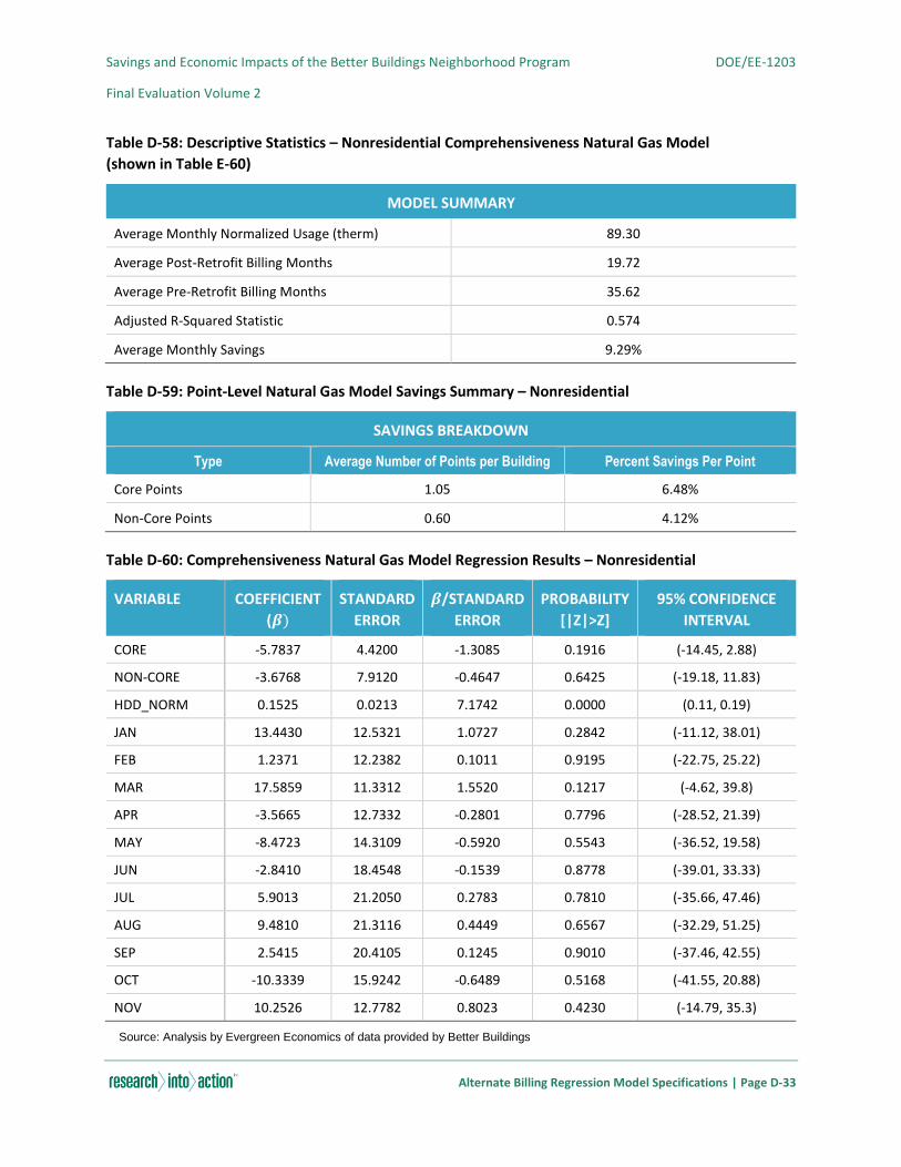
Savings and Economic Impacts of the Better Buildings Neighborhood Program DOE/EE-1203
Final Evaluation Volume 2
Alternate Billing Regression Model Specifications | Page D-33
Table D-58: Descriptive Statistics – Nonresidential Comprehensiveness Natural Gas Model
(shown in Table E-60)
MODEL SUMMARY
Average Monthly Normalized Usage (therm) 89.30
Average Post-Retrofit Billing Months 19.72
Average Pre-Retrofit Billing Months 35.62
Adjusted R-Squared Statistic 0.574
Average Monthly Savings 9.29%
Table D-59: Point-Level Natural Gas Model Savings Summary – Nonresidential
SAVINGS BREAKDOWN
Type Average Number of Points per Building Percent Savings Per Point
Core Points 1.05 6.48%
Non-Core Points 0.60 4.12%
Table D-60: Comprehensiveness Natural Gas Model Regression Results – Nonresidential
VARIABLE COEFFICIENT
(𝜷)
STANDARD
ERROR
𝜷/STANDARD
ERROR
PROBABILITY
[|Z|>Z]
95% CONFIDENCE
INTERVAL
CORE -5.7837 4.4200 -1.3085 0.1916 (-14.45, 2.88)
NON-CORE -3.6768 7.9120 -0.4647 0.6425 (-19.18, 11.83)
HDD_NORM 0.1525 0.0213 7.1742 0.0000 (0.11, 0.19)
JAN 13.4430 12.5321 1.0727 0.2842 (-11.12, 38.01)
FEB 1.2371 12.2382 0.1011 0.9195 (-22.75, 25.22)
MAR 17.5859 11.3312 1.5520 0.1217 (-4.62, 39.8)
APR -3.5665 12.7332 -0.2801 0.7796 (-28.52, 21.39)
MAY -8.4723 14.3109 -0.5920 0.5543 (-36.52, 19.58)
JUN -2.8410 18.4548 -0.1539 0.8778 (-39.01, 33.33)
JUL 5.9013 21.2050 0.2783 0.7810 (-35.66, 47.46)
AUG 9.4810 21.3116 0.4449 0.6567 (-32.29, 51.25)
SEP 2.5415 20.4105 0.1245 0.9010 (-37.46, 42.55)
OCT -10.3339 15.9242 -0.6489 0.5168 (-41.55, 20.88)
NOV 10.2526 12.7782 0.8023 0.4230 (-14.79, 35.3)
Source: Analysis by Evergreen Economics of data provided by Better Buildings
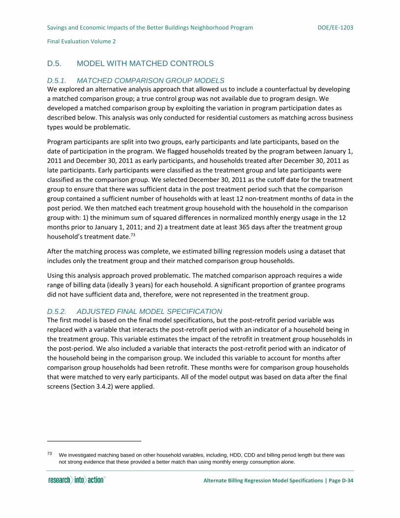
Savings and Economic Impacts of the Better Buildings Neighborhood Program DOE/EE-1203
Final Evaluation Volume 2
Alternate Billing Regression Model Specifications | Page D-34
D.5. MODEL WITH MATCHED CONTROLS
D.5.1. MATCHED COMPARISON GROUP MODELS We explored an alternative analysis approach that allowed us to include a counterfactual by developing
a matched comparison group; a true control group was not available due to program design. We
developed a matched comparison group by exploiting the variation in program participation dates as
described below. This analysis was only conducted for residential customers as matching across business
types would be problematic.
Program participants are split into two groups, early participants and late participants, based on the
date of participation in the program. We flagged households treated by the program between January 1,
2011 and December 30, 2011 as early participants, and households treated after December 30, 2011 as
late participants. Early participants were classified as the treatment group and late participants were
classified as the comparison group. We selected December 30, 2011 as the cutoff date for the treatment
group to ensure that there was sufficient data in the post treatment period such that the comparison
group contained a sufficient number of households with at least 12 non-treatment months of data in the
post period. We then matched each treatment group household with the household in the comparison
group with: 1) the minimum sum of squared differences in normalized monthly energy usage in the 12
months prior to January 1, 2011; and 2) a treatment date at least 365 days after the treatment group
household’s treatment date.73
After the matching process was complete, we estimated billing regression models using a dataset that
includes only the treatment group and their matched comparison group households.
Using this analysis approach proved problematic. The matched comparison approach requires a wide
range of billing data (ideally 3 years) for each household. A significant proportion of grantee programs
did not have sufficient data and, therefore, were not represented in the treatment group.
D.5.2. ADJUSTED FINAL MODEL SPECIFICATION The first model is based on the final model specifications, but the post-retrofit period variable was
replaced with a variable that interacts the post-retrofit period with an indicator of a household being in
the treatment group. This variable estimates the impact of the retrofit in treatment group households in
the post-period. We also included a variable that interacts the post-retrofit period with an indicator of
the household being in the comparison group. We included this variable to account for months after
comparison group households had been retrofit. These months were for comparison group households
that were matched to very early participants. All of the model output was based on data after the final
screens (Section 3.4.2) were applied.
73 We investigated matching based on other household variables, including, HDD, CDD and billing period length but there was
not strong evidence that these provided a better match than using monthly energy consumption alone.
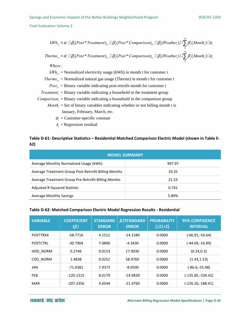
Savings and Economic Impacts of the Better Buildings Neighborhood Program DOE/EE-1203
Final Evaluation Volume 2
Alternate Billing Regression Model Specifications | Page D-35
Table D-61: Descriptive Statistics – Residential Matched Comparison Electric Model (shown in Table E-
62)
MODEL SUMMARY
Average Monthly Normalized Usage (kWh) 997.97
Average Treatment Group Post-Retrofit Billing Months 19.35
Average Treatment Group Pre-Retrofit Billing Months 21.53
Adjusted R-Squared Statistic 0.741
Average Monthly Savings 5.89%
Table D-62: Matched Comparison Electric Model Regression Results - Residential
VARIABLE COEFFICIENT
(𝜷)
STANDARD
ERROR
𝜷/STANDARD
ERROR
PROBABILITY
[|Z|>Z]
95% CONFIDENCE
INTERVAL
POSTTRXX -58.7716 4.1512 -14.1580 0.0000 (-66.91,-50.64)
POSTCTRL -30.7904 7.0896 -4.3430 0.0000 (-44.69,-16.89)
HDD_NORM 0.2746 0.0153 17.9030 0.0000 (0.24,0.3)
CDD_NORM 1.4838 0.0252 58.9760 0.0000 (1.43,1.53)
JAN -71.0381 7.9373 -8.9500 0.0000 (-86.6,-55.48)
FEB -120.1315 8.0179 -14.9830 0.0000 (-135.85,-104.42)
MAR -207.3356 9.6544 -21.4760 0.0000 (-226.26,-188.41)
kWhi,t =ai + b1(Post *Treatment)i,t + b2(Post *Comparison)i,t + b3(Weathert )+ b j (Montht )4
14
å +et
Thermsi,t =ai + b1(Post *Treatment)i,t + b2(Post *Comparison)i,t + b3(Weathert )+ b j (Montht )4
14
å +et
Where :
kWhi,t = Normalized electricity usage (kWh) in month t for customer i
Thermsi,t = Normalized natural gas usage (Therms) in month t for customer i
Posti,t = Binary variable indicating post-retrofit month for customer i
Treatmenti = Binary variable indicating a household in the treatment group
Comparisoni = Binary variable indicating a household in the comparison group
Montht = Set of binary variables indicating whether or not billing month t is
January, February, March, etc.
ai = Customer-specific constant
et = Regression residual
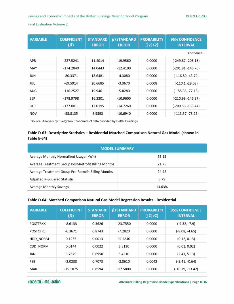
Savings and Economic Impacts of the Better Buildings Neighborhood Program DOE/EE-1203
Final Evaluation Volume 2
Alternate Billing Regression Model Specifications | Page D-36
VARIABLE COEFFICIENT
(𝜷)
STANDARD
ERROR
𝜷/STANDARD
ERROR
PROBABILITY
[|Z|>Z]
95% CONFIDENCE
INTERVAL
Continued…
APR -227.5241 11.4014 -19.9560 0.0000 (-249.87,-205.18)
MAY -174.2840 14.0443 -12.4100 0.0000 (-201.81,-146.76)
JUN -80.3371 18.6481 -4.3080 0.0000 (-116.89,-43.79)
JUL -69.5914 20.6685 -3.3670 0.0008 (-110.1,-29.08)
AUG -116.2527 19.9461 -5.8280 0.0000 (-155.35,-77.16)
SEP -178.9798 16.3301 -10.9600 0.0000 (-210.99,-146.97)
OCT -177.0011 12.0195 -14.7260 0.0000 (-200.56,-153.44)
NOV -95.8135 8.9593 -10.6940 0.0000 (-113.37,-78.25)
Source: Analysis by Evergreen Economics of data provided by Better Buildings
Table D-63: Descriptive Statistics – Residential Matched Comparison Natural Gas Model (shown in
Table E-64)
MODEL SUMMARY
Average Monthly Normalized Usage (kWh) 63.19
Average Treatment Group Post-Retrofit Billing Months 21.75
Average Treatment Group Pre-Retrofit Billing Months 24.42
Adjusted R-Squared Statistic 0.79
Average Monthly Savings 13.63%
Table D-64: Matched Comparison Natural Gas Model Regression Results - Residential
VARIABLE COEFFICIENT
(𝜷)
STANDARD
ERROR
𝜷/STANDARD
ERROR
PROBABILITY
[|Z|>Z]
95% CONFIDENCE
INTERVAL
POSTTRXX -8.6133 0.3626 -23.7550 0.0000 (-9.32, -7.9)
POSTCTRL -6.3671 0.8743 -7.2820 0.0000 (-8.08, -4.65)
HDD_NORM 0.1235 0.0013 92.2840 0.0000 (0.12, 0.13)
CDD_NORM 0.0144 0.0022 6.5130 0.0000 (0.01, 0.02)
JAN 3.7679 0.6950 5.4210 0.0000 (2.41, 5.13)
FEB -2.0238 0.7073 -2.8610 0.0042 (-3.41, -0.64)
MAR -15.1075 0.8594 -17.5800 0.0000 (-16.79, -13.42)
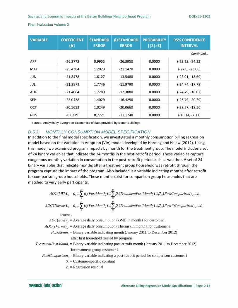
Savings and Economic Impacts of the Better Buildings Neighborhood Program DOE/EE-1203
Final Evaluation Volume 2
Alternate Billing Regression Model Specifications | Page D-37
VARIABLE COEFFICIENT
(𝜷)
STANDARD
ERROR
𝜷/STANDARD
ERROR
PROBABILITY
[|Z|>Z]
95% CONFIDENCE
INTERVAL
Continued…
APR -26.2773 0.9955 -26.3950 0.0000 (-28.23, -24.33)
MAY -25.4384 1.2029 -21.1470 0.0000 (-27.8, -23.08)
JUN -21.8478 1.6127 -13.5480 0.0000 (-25.01, -18.69)
JUL -21.2573 1.7746 -11.9790 0.0000 (-24.74, -17.78)
AUG -21.4064 1.7280 -12.3880 0.0000 (-24.79, -18.02)
SEP -23.0428 1.4029 -16.4250 0.0000 (-25.79, -20.29)
OCT -20.5652 1.0249 -20.0660 0.0000 (-22.57, -18.56)
NOV -8.6279 0.7721 -11.1740 0.0000 (-10.14, -7.11)
Source: Analysis by Evergreen Economics of data provided by Better Buildings
D.5.3. MONTHLY CONSUMPTION MODEL SPECIFICATION In addition to the final model specification, we investigated a monthly consumption billing regression
model based on the Variation in Adoption (VIA) model developed by Harding and Hsiaw (2012). Using
this model, we examined program impacts by month for the treatment group. The model includes a set
of 24 binary variables that indicate the 24 months in the post-retrofit period. These variables capture
exogenous monthly variation in consumption in the post-retrofit period such as weather. A set of 24
binary variables that indicate months after a treatment group household was retrofit through the
program capture the impact of the program. Also included is a variable indicating months after retrofit
for comparison group households. These months exist for comparison group households that are
matched to very early participants.
ADC(kWh)i,t = ai + b j (PostMontht )1
24
å + b j (TreatmentPostMontht )25
24
å + b49 (PostComparison)i,t +et
ADC(Therms)i,t = ai + b j (PostMontht )1
24
å + b j (TreatmentPostMontht )25
24
å + b49 (Post *Comparison)i,t +et
Where :
ADC(kWh)i,t = Average daily consumption (kWh) in month t for customer i
ADC(Therms)i,t = Average daily consumption (Therms) in month t for customer i
PostMontht = Binary variable indicating month (January 2011 to December 2012)
after first household treated by program
TreatmentPostMonthi = Binary variable indicating post-retrofit month (January 2011 to December 2012)
for treatment group customer i
PostComparisoni = Binary variable indicating a post-retrofit period for comparison customer i
ai = Customer-specific constant
et = Regression residual

Savings and Economic Impacts of the Better Buildings Neighborhood Program DOE/EE-1203
Final Evaluation Volume 2
Alternate Billing Regression Model Specifications | Page D-38
Table D-65: Descriptive Statistics – Residential Matched Comparison Monthly Consumption Electric
Model (shown in Table E-66)
MODEL SUMMARY
Average Monthly Normalized Usage (kWh) 997.97
Average Post-Retrofit Billing Months 19.35
Average Pre-Retrofit Billing Months 21.53
Adjusted R-Squared Statistic 0.695
Average Monthly Savings 4.81%
Table D-66: Matched Comparison Monthly Consumption Electric Model Regression Results -
Residential
VARIABLE COEFFICIENT
(𝜷)
STANDARD
ERROR
𝜷/STANDARD
ERROR
PROBABILITY
[|Z|>Z]
95% CONFIDENCE
INTERVAL
JAN11 2.2802 0.3563 6.3990 0.0000 (1.58,2.98)
FEB11 -0.0140 0.3788 -0.0370 0.9706 (-0.76,0.73)
MAR11 -4.6589 0.3842 -12.1260 0.0000 (-5.41,-3.91)
APR11 -6.3286 0.3956 -15.9960 0.0000 (-7.1,-5.55)
MAY11 -2.8701 0.4090 -7.0170 0.0000 (-3.67,-2.07)
JUN11 3.9735 0.4217 9.4220 0.0000 (3.15,4.8)
JUL11 11.0460 0.4372 25.2670 0.0000 (10.19,11.9)
AUG11 8.7433 0.4971 17.5900 0.0000 (7.77,9.72)
SEP11 -0.5754 0.5093 -1.1300 0.2586 (-1.57,0.42)
OCT11 -4.2601 0.5240 -8.1300 0.0000 (-5.29,-3.23)
NOV11 -2.8927 0.5604 -5.1620 0.0000 (-3.99,-1.79)
DEC11 1.9833 0.5649 3.5110 0.0004 (0.88,3.09)
JAN12 -0.7877 0.5669 -1.3890 0.1647 (-1.9,0.32)
FEB12 -1.5498 0.5561 -2.7870 0.0053 (-2.64,-0.46)
MAR12 -6.4293 0.5694 -11.2920 0.0000 (-7.55,-5.31)
APR12 -6.9760 0.5599 -12.4590 0.0000 (-8.07,-5.88)
MAY12 -4.6771 0.5323 -8.7870 0.0000 (-5.72,-3.63)
JUN12 6.3882 0.4763 13.4110 0.0000 (5.45,7.32)
JUL12 12.4801 0.5390 23.1560 0.0000 (11.42,13.54)
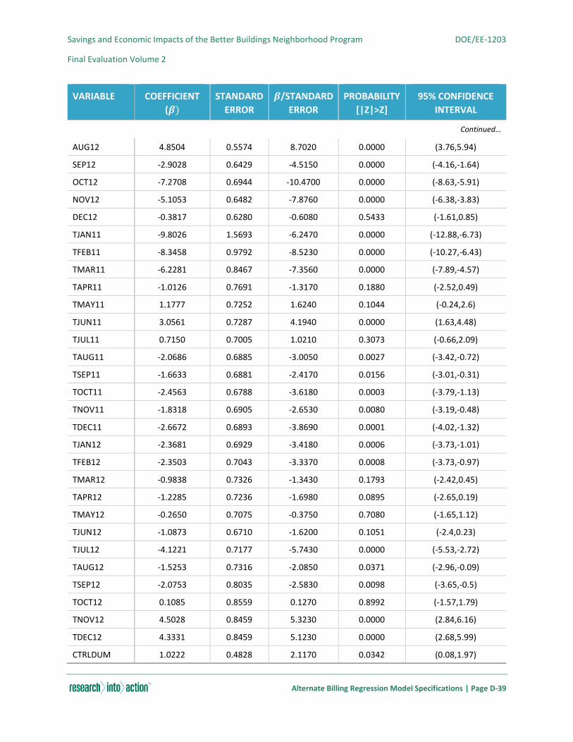
Savings and Economic Impacts of the Better Buildings Neighborhood Program DOE/EE-1203
Final Evaluation Volume 2
Alternate Billing Regression Model Specifications | Page D-39
VARIABLE COEFFICIENT
(𝜷)
STANDARD
ERROR
𝜷/STANDARD
ERROR
PROBABILITY
[|Z|>Z]
95% CONFIDENCE
INTERVAL
Continued…
AUG12 4.8504 0.5574 8.7020 0.0000 (3.76,5.94)
SEP12 -2.9028 0.6429 -4.5150 0.0000 (-4.16,-1.64)
OCT12 -7.2708 0.6944 -10.4700 0.0000 (-8.63,-5.91)
NOV12 -5.1053 0.6482 -7.8760 0.0000 (-6.38,-3.83)
DEC12 -0.3817 0.6280 -0.6080 0.5433 (-1.61,0.85)
TJAN11 -9.8026 1.5693 -6.2470 0.0000 (-12.88,-6.73)
TFEB11 -8.3458 0.9792 -8.5230 0.0000 (-10.27,-6.43)
TMAR11 -6.2281 0.8467 -7.3560 0.0000 (-7.89,-4.57)
TAPR11 -1.0126 0.7691 -1.3170 0.1880 (-2.52,0.49)
TMAY11 1.1777 0.7252 1.6240 0.1044 (-0.24,2.6)
TJUN11 3.0561 0.7287 4.1940 0.0000 (1.63,4.48)
TJUL11 0.7150 0.7005 1.0210 0.3073 (-0.66,2.09)
TAUG11 -2.0686 0.6885 -3.0050 0.0027 (-3.42,-0.72)
TSEP11 -1.6633 0.6881 -2.4170 0.0156 (-3.01,-0.31)
TOCT11 -2.4563 0.6788 -3.6180 0.0003 (-3.79,-1.13)
TNOV11 -1.8318 0.6905 -2.6530 0.0080 (-3.19,-0.48)
TDEC11 -2.6672 0.6893 -3.8690 0.0001 (-4.02,-1.32)
TJAN12 -2.3681 0.6929 -3.4180 0.0006 (-3.73,-1.01)
TFEB12 -2.3503 0.7043 -3.3370 0.0008 (-3.73,-0.97)
TMAR12 -0.9838 0.7326 -1.3430 0.1793 (-2.42,0.45)
TAPR12 -1.2285 0.7236 -1.6980 0.0895 (-2.65,0.19)
TMAY12 -0.2650 0.7075 -0.3750 0.7080 (-1.65,1.12)
TJUN12 -1.0873 0.6710 -1.6200 0.1051 (-2.4,0.23)
TJUL12 -4.1221 0.7177 -5.7430 0.0000 (-5.53,-2.72)
TAUG12 -1.5253 0.7316 -2.0850 0.0371 (-2.96,-0.09)
TSEP12 -2.0753 0.8035 -2.5830 0.0098 (-3.65,-0.5)
TOCT12 0.1085 0.8559 0.1270 0.8992 (-1.57,1.79)
TNOV12 4.5028 0.8459 5.3230 0.0000 (2.84,6.16)
TDEC12 4.3331 0.8459 5.1230 0.0000 (2.68,5.99)
CTRLDUM 1.0222 0.4828 2.1170 0.0342 (0.08,1.97)
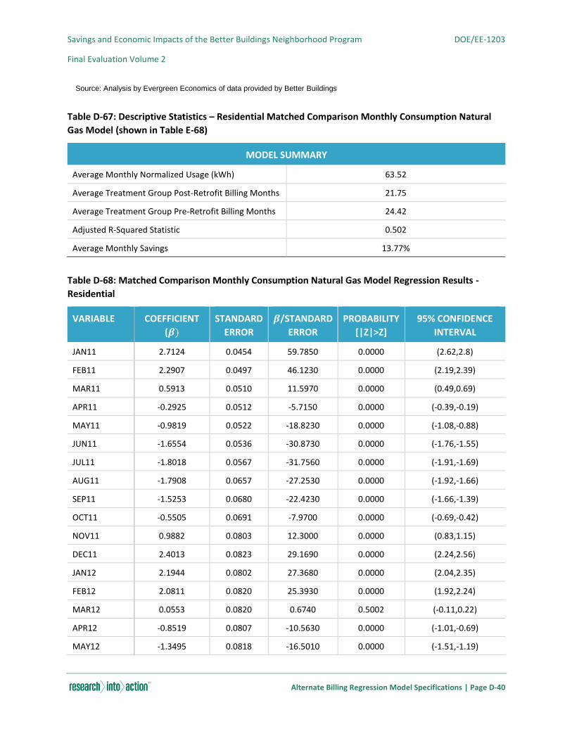
Savings and Economic Impacts of the Better Buildings Neighborhood Program DOE/EE-1203
Final Evaluation Volume 2
Alternate Billing Regression Model Specifications | Page D-40
Source: Analysis by Evergreen Economics of data provided by Better Buildings
Table D-67: Descriptive Statistics – Residential Matched Comparison Monthly Consumption Natural
Gas Model (shown in Table E-68)
MODEL SUMMARY
Average Monthly Normalized Usage (kWh) 63.52
Average Treatment Group Post-Retrofit Billing Months 21.75
Average Treatment Group Pre-Retrofit Billing Months 24.42
Adjusted R-Squared Statistic 0.502
Average Monthly Savings 13.77%
Table D-68: Matched Comparison Monthly Consumption Natural Gas Model Regression Results -
Residential
VARIABLE COEFFICIENT
(𝜷)
STANDARD
ERROR
𝜷/STANDARD
ERROR
PROBABILITY
[|Z|>Z]
95% CONFIDENCE
INTERVAL
JAN11 2.7124 0.0454 59.7850 0.0000 (2.62,2.8)
FEB11 2.2907 0.0497 46.1230 0.0000 (2.19,2.39)
MAR11 0.5913 0.0510 11.5970 0.0000 (0.49,0.69)
APR11 -0.2925 0.0512 -5.7150 0.0000 (-0.39,-0.19)
MAY11 -0.9819 0.0522 -18.8230 0.0000 (-1.08,-0.88)
JUN11 -1.6554 0.0536 -30.8730 0.0000 (-1.76,-1.55)
JUL11 -1.8018 0.0567 -31.7560 0.0000 (-1.91,-1.69)
AUG11 -1.7908 0.0657 -27.2530 0.0000 (-1.92,-1.66)
SEP11 -1.5253 0.0680 -22.4230 0.0000 (-1.66,-1.39)
OCT11 -0.5505 0.0691 -7.9700 0.0000 (-0.69,-0.42)
NOV11 0.9882 0.0803 12.3000 0.0000 (0.83,1.15)
DEC11 2.4013 0.0823 29.1690 0.0000 (2.24,2.56)
JAN12 2.1944 0.0802 27.3680 0.0000 (2.04,2.35)
FEB12 2.0811 0.0820 25.3930 0.0000 (1.92,2.24)
MAR12 0.0553 0.0820 0.6740 0.5002 (-0.11,0.22)
APR12 -0.8519 0.0807 -10.5630 0.0000 (-1.01,-0.69)
MAY12 -1.3495 0.0818 -16.5010 0.0000 (-1.51,-1.19)
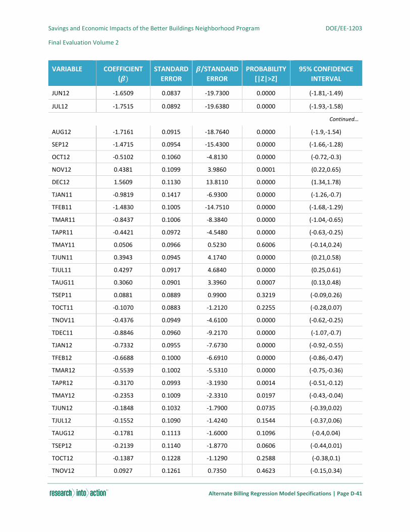
Savings and Economic Impacts of the Better Buildings Neighborhood Program DOE/EE-1203
Final Evaluation Volume 2
Alternate Billing Regression Model Specifications | Page D-41
VARIABLE COEFFICIENT
(𝜷)
STANDARD
ERROR
𝜷/STANDARD
ERROR
PROBABILITY
[|Z|>Z]
95% CONFIDENCE
INTERVAL
JUN12 -1.6509 0.0837 -19.7300 0.0000 (-1.81,-1.49)
JUL12 -1.7515 0.0892 -19.6380 0.0000 (-1.93,-1.58)
Continued…
AUG12 -1.7161 0.0915 -18.7640 0.0000 (-1.9,-1.54)
SEP12 -1.4715 0.0954 -15.4300 0.0000 (-1.66,-1.28)
OCT12 -0.5102 0.1060 -4.8130 0.0000 (-0.72,-0.3)
NOV12 0.4381 0.1099 3.9860 0.0001 (0.22,0.65)
DEC12 1.5609 0.1130 13.8110 0.0000 (1.34,1.78)
TJAN11 -0.9819 0.1417 -6.9300 0.0000 (-1.26,-0.7)
TFEB11 -1.4830 0.1005 -14.7510 0.0000 (-1.68,-1.29)
TMAR11 -0.8437 0.1006 -8.3840 0.0000 (-1.04,-0.65)
TAPR11 -0.4421 0.0972 -4.5480 0.0000 (-0.63,-0.25)
TMAY11 0.0506 0.0966 0.5230 0.6006 (-0.14,0.24)
TJUN11 0.3943 0.0945 4.1740 0.0000 (0.21,0.58)
TJUL11 0.4297 0.0917 4.6840 0.0000 (0.25,0.61)
TAUG11 0.3060 0.0901 3.3960 0.0007 (0.13,0.48)
TSEP11 0.0881 0.0889 0.9900 0.3219 (-0.09,0.26)
TOCT11 -0.1070 0.0883 -1.2120 0.2255 (-0.28,0.07)
TNOV11 -0.4376 0.0949 -4.6100 0.0000 (-0.62,-0.25)
TDEC11 -0.8846 0.0960 -9.2170 0.0000 (-1.07,-0.7)
TJAN12 -0.7332 0.0955 -7.6730 0.0000 (-0.92,-0.55)
TFEB12 -0.6688 0.1000 -6.6910 0.0000 (-0.86,-0.47)
TMAR12 -0.5539 0.1002 -5.5310 0.0000 (-0.75,-0.36)
TAPR12 -0.3170 0.0993 -3.1930 0.0014 (-0.51,-0.12)
TMAY12 -0.2353 0.1009 -2.3310 0.0197 (-0.43,-0.04)
TJUN12 -0.1848 0.1032 -1.7900 0.0735 (-0.39,0.02)
TJUL12 -0.1552 0.1090 -1.4240 0.1544 (-0.37,0.06)
TAUG12 -0.1781 0.1113 -1.6000 0.1096 (-0.4,0.04)
TSEP12 -0.2139 0.1140 -1.8770 0.0606 (-0.44,0.01)
TOCT12 -0.1387 0.1228 -1.1290 0.2588 (-0.38,0.1)
TNOV12 0.0927 0.1261 0.7350 0.4623 (-0.15,0.34)
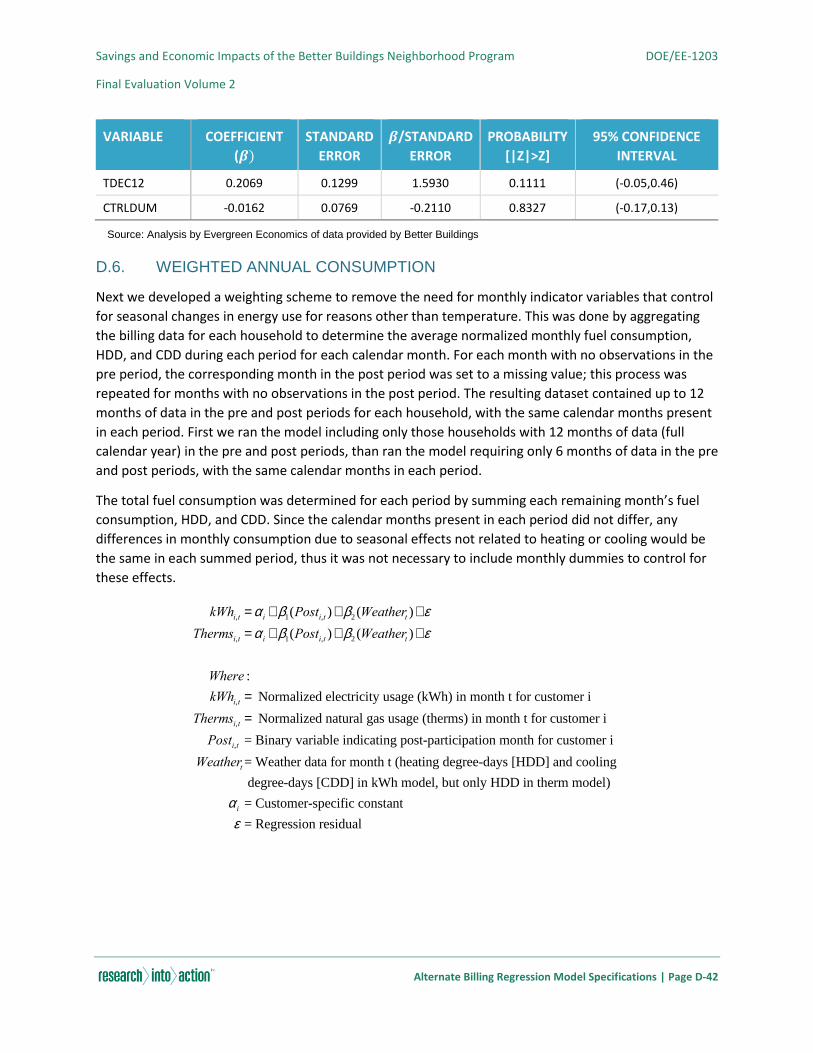
Savings and Economic Impacts of the Better Buildings Neighborhood Program DOE/EE-1203
Final Evaluation Volume 2
Alternate Billing Regression Model Specifications | Page D-42
VARIABLE COEFFICIENT
(𝜷)
STANDARD
ERROR
𝜷/STANDARD
ERROR
PROBABILITY
[|Z|>Z]
95% CONFIDENCE
INTERVAL
TDEC12 0.2069 0.1299 1.5930 0.1111 (-0.05,0.46)
CTRLDUM -0.0162 0.0769 -0.2110 0.8327 (-0.17,0.13)
Source: Analysis by Evergreen Economics of data provided by Better Buildings
D.6. WEIGHTED ANNUAL CONSUMPTION
Next we developed a weighting scheme to remove the need for monthly indicator variables that control
for seasonal changes in energy use for reasons other than temperature. This was done by aggregating
the billing data for each household to determine the average normalized monthly fuel consumption,
HDD, and CDD during each period for each calendar month. For each month with no observations in the
pre period, the corresponding month in the post period was set to a missing value; this process was
repeated for months with no observations in the post period. The resulting dataset contained up to 12
months of data in the pre and post periods for each household, with the same calendar months present
in each period. First we ran the model including only those households with 12 months of data (full
calendar year) in the pre and post periods, than ran the model requiring only 6 months of data in the pre
and post periods, with the same calendar months in each period.
The total fuel consumption was determined for each period by summing each remaining month’s fuel
consumption, HDD, and CDD. Since the calendar months present in each period did not differ, any
differences in monthly consumption due to seasonal effects not related to heating or cooling would be
the same in each summed period, thus it was not necessary to include monthly dummies to control for
these effects.
kWhi,t = ai + b1(Posti,t )+ b2 (Weathert )+e
Thermsi,t = ai + b1(Posti,t )+ b2 (Weathert )+e
Where :
kWhi,t = Normalized electricity usage (kWh) in month t for customer i
Thermsi,t = Normalized natural gas usage (therms) in month t for customer i
Posti,t = Binary variable indicating post-participation month for customer i
Weathert= Weather data for month t (heating degree-days [HDD] and cooling
degree-days [CDD] in kWh model, but only HDD in therm model)
ai = Customer-specific constant
e = Regression residual
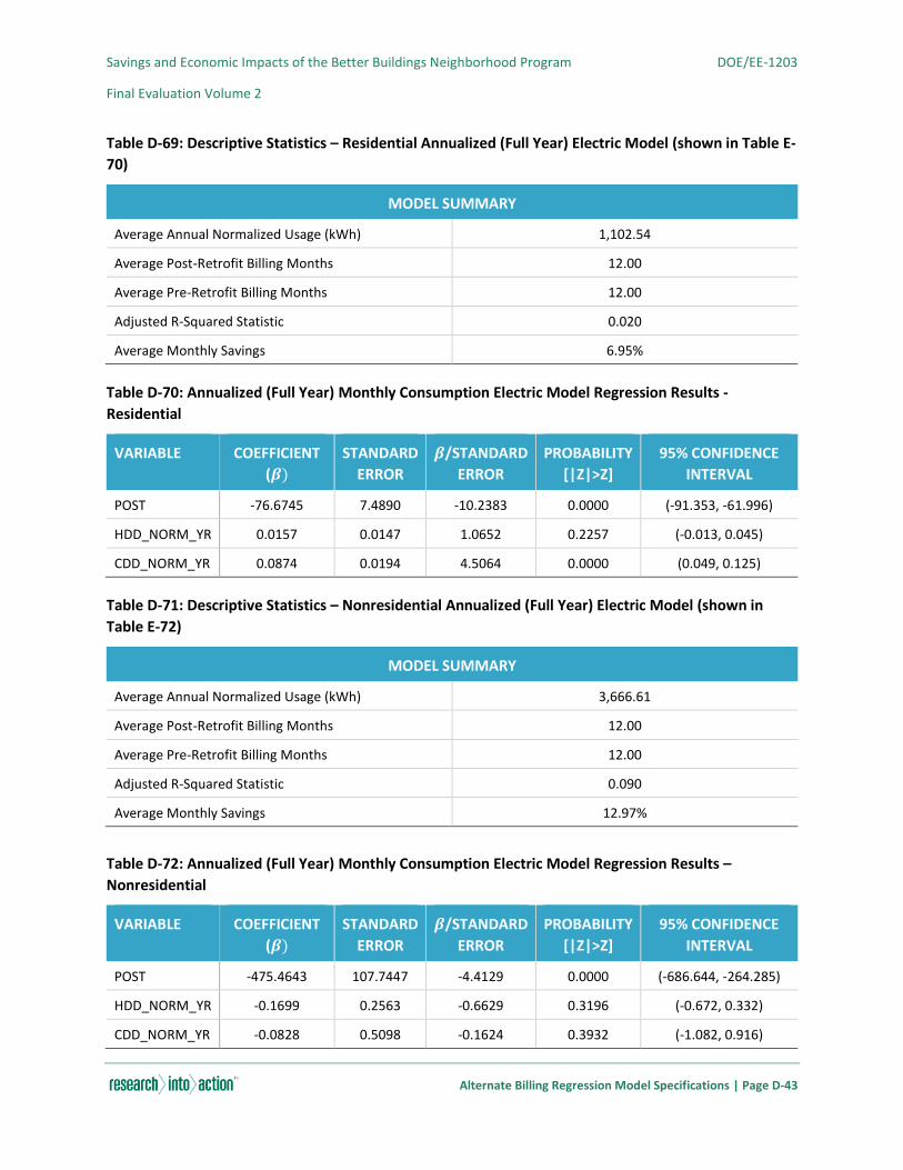
Savings and Economic Impacts of the Better Buildings Neighborhood Program DOE/EE-1203
Final Evaluation Volume 2
Alternate Billing Regression Model Specifications | Page D-43
Table D-69: Descriptive Statistics – Residential Annualized (Full Year) Electric Model (shown in Table E-
70)
MODEL SUMMARY
Average Annual Normalized Usage (kWh) 1,102.54
Average Post-Retrofit Billing Months 12.00
Average Pre-Retrofit Billing Months 12.00
Adjusted R-Squared Statistic 0.020
Average Monthly Savings 6.95%
Table D-70: Annualized (Full Year) Monthly Consumption Electric Model Regression Results -
Residential
VARIABLE COEFFICIENT
(𝜷)
STANDARD
ERROR
𝜷/STANDARD
ERROR
PROBABILITY
[|Z|>Z]
95% CONFIDENCE
INTERVAL
POST -76.6745 7.4890 -10.2383 0.0000 (-91.353, -61.996)
HDD_NORM_YR 0.0157 0.0147 1.0652 0.2257 (-0.013, 0.045)
CDD_NORM_YR 0.0874 0.0194 4.5064 0.0000 (0.049, 0.125)
Table D-71: Descriptive Statistics – Nonresidential Annualized (Full Year) Electric Model (shown in
Table E-72)
MODEL SUMMARY
Average Annual Normalized Usage (kWh) 3,666.61
Average Post-Retrofit Billing Months 12.00
Average Pre-Retrofit Billing Months 12.00
Adjusted R-Squared Statistic 0.090
Average Monthly Savings 12.97%
Table D-72: Annualized (Full Year) Monthly Consumption Electric Model Regression Results –
Nonresidential
VARIABLE COEFFICIENT
(𝜷)
STANDARD
ERROR
𝜷/STANDARD
ERROR
PROBABILITY
[|Z|>Z]
95% CONFIDENCE
INTERVAL
POST -475.4643 107.7447 -4.4129 0.0000 (-686.644, -264.285)
HDD_NORM_YR -0.1699 0.2563 -0.6629 0.3196 (-0.672, 0.332)
CDD_NORM_YR -0.0828 0.5098 -0.1624 0.3932 (-1.082, 0.916)

Savings and Economic Impacts of the Better Buildings Neighborhood Program DOE/EE-1203
Final Evaluation Volume 2
Alternate Billing Regression Model Specifications | Page D-44
Table D-73: Descriptive Statistics – Residential Annualized (Full Year) Natural Gas Model (shown in
Table E-74)
MODEL SUMMARY
Average Annual Normalized Usage (therms) 71.13
Average Post-Retrofit Billing Months 12.00
Average Pre-Retrofit Billing Months 12.00
Adjusted R-Squared Statistic 0.131
Average Monthly Savings 11.77%
Table D-74: Annualized (Full Year) Monthly Consumption Natural Gas Model Regression Results –
Residential
VARIABLE COEFFICIENT
(𝜷)
STANDARD
ERROR
𝜷/STANDARD
ERROR
PROBABILITY
[|Z|>Z]
95% CONFIDENCE
INTERVAL
POST -8.3714 0.4459 -18.7721 0.0000 (-9.245, -7.497)
HDD_NORM_YR 0.0165 0.0010 17.2553 0.0000 (0.015, 0.018)
Table D-75: Descriptive Statistics – Nonresidential Annualized (Full Year) Natural Gas Model (shown in
Table E-76)
MODEL SUMMARY
Average Annual Normalized Usage (therms) 145.08
Average Post-Retrofit Billing Months 12.00
Average Pre-Retrofit Billing Months 12.00
Adjusted R-Squared Statistic 0.042
Average Monthly Savings -7.26%
Table D-76: Annualized (Full Year) Monthly Consumption Natural Gas Model Regression Results –
Nonresidential
VARIABLE COEFFICIENT
(𝜷)
STANDARD
ERROR
𝜷/STANDARD
ERROR
PROBABILITY
[|Z|>Z]
95% CONFIDENCE
INTERVAL
POST 10.5366 5.3569 1.9669 0.0581 (0.037, 21.036)
HDD_NORM_YR 0.0386 0.0152 2.5423 0.0163 (0.009, 0.068)
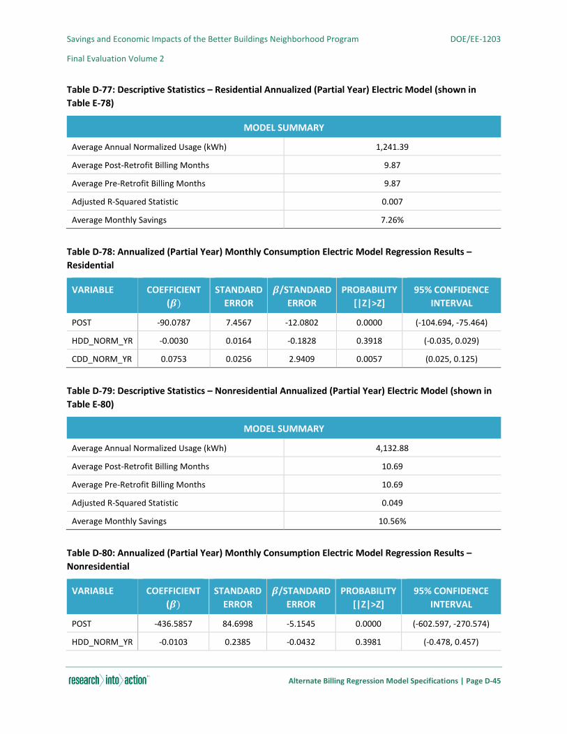
Savings and Economic Impacts of the Better Buildings Neighborhood Program DOE/EE-1203
Final Evaluation Volume 2
Alternate Billing Regression Model Specifications | Page D-45
Table D-77: Descriptive Statistics – Residential Annualized (Partial Year) Electric Model (shown in
Table E-78)
MODEL SUMMARY
Average Annual Normalized Usage (kWh) 1,241.39
Average Post-Retrofit Billing Months 9.87
Average Pre-Retrofit Billing Months 9.87
Adjusted R-Squared Statistic 0.007
Average Monthly Savings 7.26%
Table D-78: Annualized (Partial Year) Monthly Consumption Electric Model Regression Results –
Residential
VARIABLE COEFFICIENT
(𝜷)
STANDARD
ERROR
𝜷/STANDARD
ERROR
PROBABILITY
[|Z|>Z]
95% CONFIDENCE
INTERVAL
POST -90.0787 7.4567 -12.0802 0.0000 (-104.694, -75.464)
HDD_NORM_YR -0.0030 0.0164 -0.1828 0.3918 (-0.035, 0.029)
CDD_NORM_YR 0.0753 0.0256 2.9409 0.0057 (0.025, 0.125)
Table D-79: Descriptive Statistics – Nonresidential Annualized (Partial Year) Electric Model (shown in
Table E-80)
MODEL SUMMARY
Average Annual Normalized Usage (kWh) 4,132.88
Average Post-Retrofit Billing Months 10.69
Average Pre-Retrofit Billing Months 10.69
Adjusted R-Squared Statistic 0.049
Average Monthly Savings 10.56%
Table D-80: Annualized (Partial Year) Monthly Consumption Electric Model Regression Results –
Nonresidential
VARIABLE COEFFICIENT
(𝜷)
STANDARD
ERROR
𝜷/STANDARD
ERROR
PROBABILITY
[|Z|>Z]
95% CONFIDENCE
INTERVAL
POST -436.5857 84.6998 -5.1545 0.0000 (-602.597, -270.574)
HDD_NORM_YR -0.0103 0.2385 -0.0432 0.3981 (-0.478, 0.457)
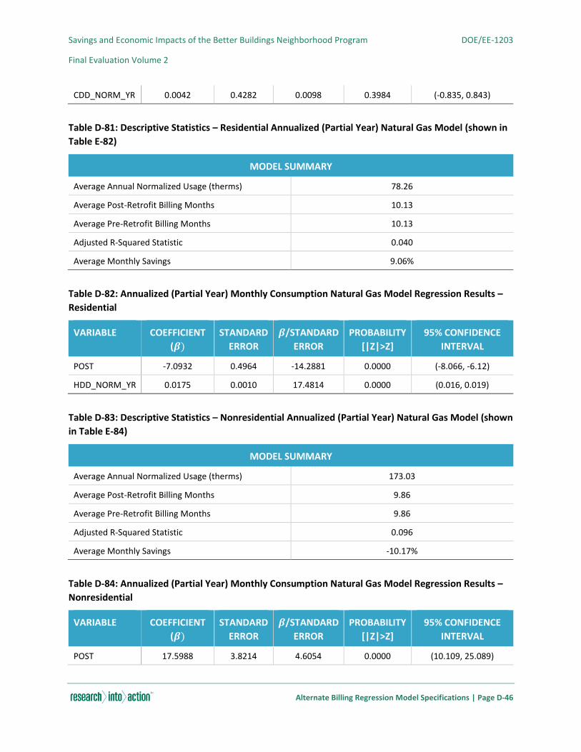
Savings and Economic Impacts of the Better Buildings Neighborhood Program DOE/EE-1203
Final Evaluation Volume 2
Alternate Billing Regression Model Specifications | Page D-46
CDD_NORM_YR 0.0042 0.4282 0.0098 0.3984 (-0.835, 0.843)
Table D-81: Descriptive Statistics – Residential Annualized (Partial Year) Natural Gas Model (shown in
Table E-82)
MODEL SUMMARY
Average Annual Normalized Usage (therms) 78.26
Average Post-Retrofit Billing Months 10.13
Average Pre-Retrofit Billing Months 10.13
Adjusted R-Squared Statistic 0.040
Average Monthly Savings 9.06%
Table D-82: Annualized (Partial Year) Monthly Consumption Natural Gas Model Regression Results –
Residential
VARIABLE COEFFICIENT
(𝜷)
STANDARD
ERROR
𝜷/STANDARD
ERROR
PROBABILITY
[|Z|>Z]
95% CONFIDENCE
INTERVAL
POST -7.0932 0.4964 -14.2881 0.0000 (-8.066, -6.12)
HDD_NORM_YR 0.0175 0.0010 17.4814 0.0000 (0.016, 0.019)
Table D-83: Descriptive Statistics – Nonresidential Annualized (Partial Year) Natural Gas Model (shown
in Table E-84)
MODEL SUMMARY
Average Annual Normalized Usage (therms) 173.03
Average Post-Retrofit Billing Months 9.86
Average Pre-Retrofit Billing Months 9.86
Adjusted R-Squared Statistic 0.096
Average Monthly Savings -10.17%
Table D-84: Annualized (Partial Year) Monthly Consumption Natural Gas Model Regression Results –
Nonresidential
VARIABLE COEFFICIENT
(𝜷)
STANDARD
ERROR
𝜷/STANDARD
ERROR
PROBABILITY
[|Z|>Z]
95% CONFIDENCE
INTERVAL
POST 17.5988 3.8214 4.6054 0.0000 (10.109, 25.089)

Savings and Economic Impacts of the Better Buildings Neighborhood Program DOE/EE-1203
Final Evaluation Volume 2
Alternate Billing Regression Model Specifications | Page D-47
HDD_NORM_YR 0.0505 0.0094 5.3531 0.0000 (0.032, 0.069)
D.7. NORMALIZED ANNUAL CONSUMPTION
The next model we used was normalized annual consumption model, which normalizes the
consumption during each period before comparing the pre and post, instead of determining the heating
and cooling slopes in the same model as the other components of consumption. The first step in this
process was to run grantee-level models with pre-period data to determine the household baseline
consumption (intercepts), heating slope, and cooling slope for each household. Then the post-period
annual consumption was estimated using the known HDD and CDD in the post-period multiplied by their
heating and cooling slopes, respectively, then adding the household’s monthly baseline consumption
multiplied by 12. Then the expected difference between the pre-period and the post-period was
determined by subtracting the pre-period consumption from the expected post-period consumption.
The actual difference between the pre- and post-period represents the impact of participation. So we
included the expected difference as Part=0 and the observed difference as Part=1. The final model used
this data to determine the impact of participation in the program with the coefficient on the Part
variable.
Table D-85: Descriptive Statistics – Residential Normalized Annual Electric Model (shown in Table E-
86)
MODEL SUMMARY
Average Annual Normalized Usage (kWh) 13,933.55
Average Post-Retrofit Billing Months 16.47
Average Pre-Retrofit Billing Months 22.75
Adjusted R-Squared Statistic 0.012
Average Monthly Savings 9.52%
Table D-86: Normalized Annual Consumption Electric Model Regression Results – Residential
VARIABLE COEFFICIENT
(𝜷)
STANDARD
ERROR
𝜷/STANDARD
ERROR
PROBABILITY
[|Z|>Z]
95% CONFIDENCE
INTERVAL
PART -1327.0300 128.9600 -10.2902 0.0000 (-1579.792, -1074.268)
Normalized Annual Consumption:
Fueli,t = mi + bw(Weathert )+e
NACi,t = (12 ´mi )+ (b̂w ´Weathert )
DNACi,t =ai + bP (Parti )+e
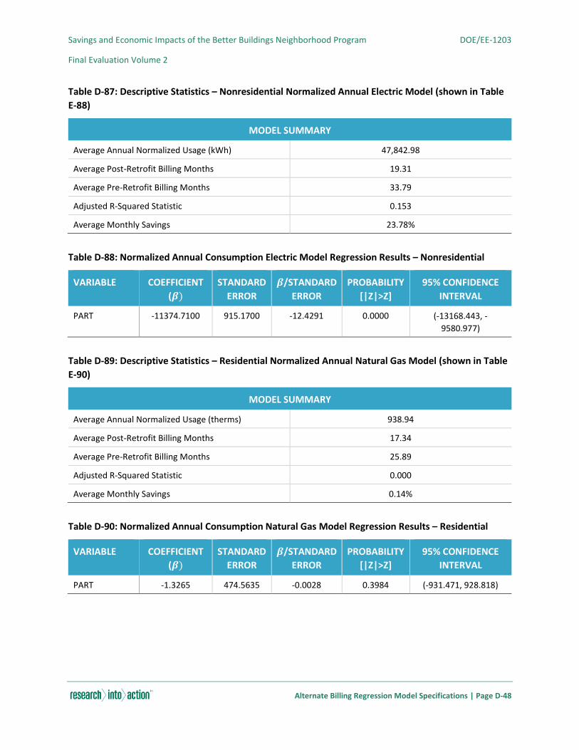
Savings and Economic Impacts of the Better Buildings Neighborhood Program DOE/EE-1203
Final Evaluation Volume 2
Alternate Billing Regression Model Specifications | Page D-48
Table D-87: Descriptive Statistics – Nonresidential Normalized Annual Electric Model (shown in Table
E-88)
MODEL SUMMARY
Average Annual Normalized Usage (kWh) 47,842.98
Average Post-Retrofit Billing Months 19.31
Average Pre-Retrofit Billing Months 33.79
Adjusted R-Squared Statistic 0.153
Average Monthly Savings 23.78%
Table D-88: Normalized Annual Consumption Electric Model Regression Results – Nonresidential
VARIABLE COEFFICIENT
(𝜷)
STANDARD
ERROR
𝜷/STANDARD
ERROR
PROBABILITY
[|Z|>Z]
95% CONFIDENCE
INTERVAL
PART -11374.7100 915.1700 -12.4291 0.0000 (-13168.443, -
9580.977)
Table D-89: Descriptive Statistics – Residential Normalized Annual Natural Gas Model (shown in Table
E-90)
MODEL SUMMARY
Average Annual Normalized Usage (therms) 938.94
Average Post-Retrofit Billing Months 17.34
Average Pre-Retrofit Billing Months 25.89
Adjusted R-Squared Statistic 0.000
Average Monthly Savings 0.14%
Table D-90: Normalized Annual Consumption Natural Gas Model Regression Results – Residential
VARIABLE COEFFICIENT
(𝜷)
STANDARD
ERROR
𝜷/STANDARD
ERROR
PROBABILITY
[|Z|>Z]
95% CONFIDENCE
INTERVAL
PART -1.3265 474.5635 -0.0028 0.3984 (-931.471, 928.818)
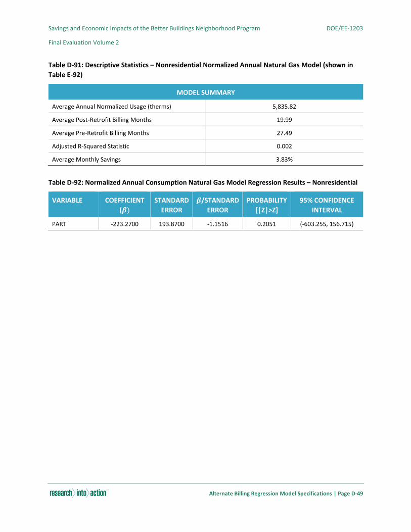
Savings and Economic Impacts of the Better Buildings Neighborhood Program DOE/EE-1203
Final Evaluation Volume 2
Alternate Billing Regression Model Specifications | Page D-49
Table D-91: Descriptive Statistics – Nonresidential Normalized Annual Natural Gas Model (shown in
Table E-92)
MODEL SUMMARY
Average Annual Normalized Usage (therms) 5,835.82
Average Post-Retrofit Billing Months 19.99
Average Pre-Retrofit Billing Months 27.49
Adjusted R-Squared Statistic 0.002
Average Monthly Savings 3.83%
Table D-92: Normalized Annual Consumption Natural Gas Model Regression Results – Nonresidential
VARIABLE COEFFICIENT
(𝜷)
STANDARD
ERROR
𝜷/STANDARD
ERROR
PROBABILITY
[|Z|>Z]
95% CONFIDENCE
INTERVAL
PART -223.2700 193.8700 -1.1516 0.2051 (-603.255, 156.715)

Savings and Economic Impacts of the Better Buildings Neighborhood Program DOE/EE-1203
Final Evaluation Volume 2
Alternative Billing Data Screens | Page E-1
APPENDIX E. ALTERNATIVE BILLING DATA SCREENS
Once all data were received from the grantees, we developed data screens to clean the billing data for
analysis. The goal of screening is to remove any potentially erroneous billing data from the final
modeling dataset to avoid biasing the estimation results. Though a variety of data screens were tried on
the models as a sensitivity test, none altered the results or statistical significance of the results greatly,
so we opted to use the data screens explained in Appendix B.4.2.
Table E-1 provides a definition of the different electric filters that we used, and Table E-4 provides a
definition of the different natural gas filters that we used. Table E-2 and Table E-3 provide summaries of
the model output for each of these electric filters for residential and commercial buildings, and Table E-5
and Table E-6 provide the model output summaries for each of the natural gas filters for residential and
commercial buildings.
Table E-1: Electric Model Filter Definitions
FILTER REQUIREMENTS
NONE N/A
MIN BILLS PRE_SUM>=12 & POST_SUM>0
RELIABLE BILLS BILLDAYS>=28 & BILLDAYS<=35 & NORM_FUELQTY>=100 & NORM_FUELQTY<=10000
PRELIMINARY PRE_SUM>=12 & POST_SUM>0 & BILLDAYS>=28 & BILLDAYS<=35 & NORM_FUELQTY>=100 &
NORM_FUELQTY<=10000
MORE POST PRE_SUM>=12 & POST_SUM>=6 & BILLDAYS>=28 & BILLDAYS<=35 & NORM_FUELQTY>=100
& NORM_FUELQTY<=10000
EVEN MORE
POST
PRE_SUM>=12 & POST_SUM>=12 & BILLDAYS>=28 & BILLDAYS<=35 &
NORM_FUELQTY>=100 & NORM_FUELQTY<=10000
CONSISTENT
BILLS
PRE_MEAN_NORM_FUELQTY>=200 & PRE_MEAN_NORM_FUELQTY<=5000 & PRE_SUM>=12
& POST_SUM>=12 & BILLDAYS>=28 & BILLDAYS<=35 & NORM_FUELQTY>=100 &
NORM_FUELQTY<=10000
NO DRAMATIC
INCREASE
PCT_CHANGE_MEANQTY<1 & PRE_MEAN_NORM_FUELQTY>=200 &
PRE_MEAN_NORM_FUELQTY<=5000 & PRE_SUM>=12 & POST_SUM>=12 & BILLDAYS>=28 &
BILLDAYS<=35 & NORM_FUELQTY>=100 & NORM_FUELQTY<=10000
REQUIRE
INSTALLATIONS
FLAG_ELECT_SAVINGS==1 & PCT_CHANGE_MEANQTY<1 &
PRE_MEAN_NORM_FUELQTY>=200 & PRE_MEAN_NORM_FUELQTY<=5000 & PRE_SUM>=12
& POST_SUM>=12 & BILLDAYS>=28 & BILLDAYS<=35 & NORM_FUELQTY>=100 &
NORM_FUELQTY<=10000

Savings and Economic Impacts of the Better Buildings Neighborhood Program DOE/EE-1203
Final Evaluation Volume 2
Alternative Billing Data Screens | Page E-2
Table E-2: Electric Regression Results with Different Filters – Residential
FILTER RESIDENTIAL MODEL SUMMARY
OBS HH POST COEFF (β)
STND ERROR
PROB [|Z|>z]
95% CI ADJ R2 MEAN USAGE (kWh)
PERCENT SAVINGS
NONE 581,529 20,879 -
118.993
32.201 0.0002 (-182.11,
-55.88)
0.0005 1,024.61 11.6%
MIN BILLS 485,026 15,262 -
120.575
37.439 0.0013 (-193.96,
-47.19)
0.0004 1,032.16 11.7%
RELIABLE BILLS 508,254 19,289 -83.073 1.348 0.0000 (-85.72,
-80.43)
0.2255 1,001.15 8.3%
PRELIMINARY 417,307 13,743 -82.523 1.456 0.0000 (-85.38,
-79.67)
0.2203 1,003.78 8.2%
MORE POST 305,128 9,124 -80.946 1.547 0.0000 (-83.98,
-77.91)
0.2069 1,016.86 8.0%
EVEN MORE
POST
183,491 4,845 -66.007 1.866 0.0000 (-69.66,
-62.35)
0.2089 1,053.87 6.3%
CONSISTENT
BILLS
176,839 4,666 -60.598 1.796 0.0000 (-64.12,
-57.08)
0.2372 931.42 6.5%
NO DRAMATIC
INCREASE
174,468 4,599 -70.920 1.773 0.0000 (-74.39,
-67.45)
0.2466 927.79 7.6%
REQUIRE
INSTALLATIONS
160,199 4,220 -76.273 1.849 0.0000 (-79.9,
-72.65)
0.2570 938.61 8.1%
Table E-3: Electric Regression Results with Different Filters – Nonresidential
FILTER NONRESIDENTIAL MODEL SUMMARY
OBS HH POST COEFF (β)
STND ERROR
PROB [|Z|>z]
95% CI ADJ R2 MEAN USAGE (kWh)
PERCENT SAVINGS
NONE 61,462 1,352 -
5639.03
752.574 0.0000 (-7114.1,
-4164.0)
0.0142 61,979.9 9.1%
MIN BILLS 53,792 1,051 -
5794.26
767.555 0.0000 (-7298.7,
-4289.9
0.0126 58,599.1 9.9%
RELIABLE BILLS 36,869 1,035 -
403.675
14.233 0.0000 (-431.6,
-375.8)
0.1829 3,624.2 11.1%
Continued…
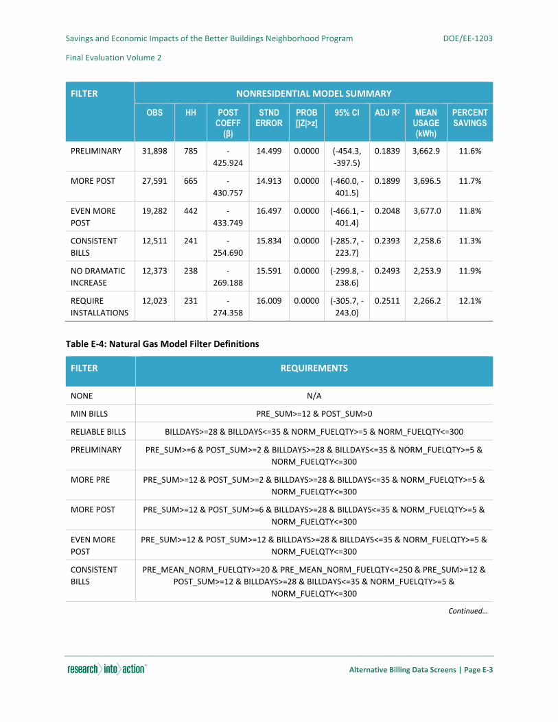
Savings and Economic Impacts of the Better Buildings Neighborhood Program DOE/EE-1203
Final Evaluation Volume 2
Alternative Billing Data Screens | Page E-3
FILTER NONRESIDENTIAL MODEL SUMMARY
OBS HH POST COEFF (β)
STND ERROR
PROB [|Z|>z]
95% CI ADJ R2 MEAN USAGE (kWh)
PERCENT SAVINGS
PRELIMINARY 31,898 785 -
425.924
14.499 0.0000 (-454.3,
-397.5)
0.1839 3,662.9 11.6%
MORE POST 27,591 665 -
430.757
14.913 0.0000 (-460.0, -
401.5)
0.1899 3,696.5 11.7%
EVEN MORE
POST
19,282 442 -
433.749
16.497 0.0000 (-466.1, -
401.4)
0.2048 3,677.0 11.8%
CONSISTENT
BILLS
12,511 241 -
254.690
15.834 0.0000 (-285.7, -
223.7)
0.2393 2,258.6 11.3%
NO DRAMATIC
INCREASE
12,373 238 -
269.188
15.591 0.0000 (-299.8, -
238.6)
0.2493 2,253.9 11.9%
REQUIRE
INSTALLATIONS
12,023 231 -
274.358
16.009 0.0000 (-305.7, -
243.0)
0.2511 2,266.2 12.1%
Table E-4: Natural Gas Model Filter Definitions
FILTER REQUIREMENTS
NONE N/A
MIN BILLS PRE_SUM>=12 & POST_SUM>0
RELIABLE BILLS BILLDAYS>=28 & BILLDAYS<=35 & NORM_FUELQTY>=5 & NORM_FUELQTY<=300
PRELIMINARY PRE_SUM>=6 & POST_SUM>=2 & BILLDAYS>=28 & BILLDAYS<=35 & NORM_FUELQTY>=5 &
NORM_FUELQTY<=300
MORE PRE PRE_SUM>=12 & POST_SUM>=2 & BILLDAYS>=28 & BILLDAYS<=35 & NORM_FUELQTY>=5 &
NORM_FUELQTY<=300
MORE POST PRE_SUM>=12 & POST_SUM>=6 & BILLDAYS>=28 & BILLDAYS<=35 & NORM_FUELQTY>=5 &
NORM_FUELQTY<=300
EVEN MORE
POST
PRE_SUM>=12 & POST_SUM>=12 & BILLDAYS>=28 & BILLDAYS<=35 & NORM_FUELQTY>=5 &
NORM_FUELQTY<=300
CONSISTENT
BILLS
PRE_MEAN_NORM_FUELQTY>=20 & PRE_MEAN_NORM_FUELQTY<=250 & PRE_SUM>=12 &
POST_SUM>=12 & BILLDAYS>=28 & BILLDAYS<=35 & NORM_FUELQTY>=5 &
NORM_FUELQTY<=300
Continued…
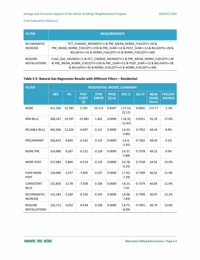
Savings and Economic Impacts of the Better Buildings Neighborhood Program DOE/EE-1203
Final Evaluation Volume 2
Alternative Billing Data Screens | Page E-4
FILTER REQUIREMENTS
NO DRAMATIC
INCREASE
PCT_CHANGE_MEANQTY<1 & PRE_MEAN_NORM_FUELQTY>=20 &
PRE_MEAN_NORM_FUELQTY<=250 & PRE_SUM>=12 & POST_SUM>=12 & BILLDAYS>=28 &
BILLDAYS<=35 & NORM_FUELQTY>=5 & NORM_FUELQTY<=300
REQUIRE
INSTALLATIONS
FLAG_GAS_SAVINGS==1 & PCT_CHANGE_MEANQTY<1 & PRE_MEAN_NORM_FUELQTY>=20
& PRE_MEAN_NORM_FUELQTY<=250 & PRE_SUM>=12 & POST_SUM>=12 & BILLDAYS>=28
& BILLDAYS<=35 & NORM_FUELQTY>=5 & NORM_FUELQTY<=300
Table E-5: Natural Gas Regression Results with Different Filters – Residential
FILTER RESIDENTIAL MODEL SUMMARY
OBS HH POST COEFF (β)
STND ERROR
PROB [|Z|>z]
95% CI ADJ R2 MEAN USAGE (therm)
PERCENT SAVINGS
NONE 411,566 12,783 2.293 10.113 0.8207 (-17.53,
22.12)
0.0045 173.77 -1.3%
MIN BILLS 368,167 10,297 -15.482 1.461 0.0000 (-18.35,
-12.62)
0.0321 91.29 17.0%
RELIABLE BILLS 365,006 12,226 -6.097 0.121 0.0000 (-6.33,
-5.86)
0.7352 68.26 8.9%
PRELIMINARY 326,652 9,840 -6.162 0.123 0.0000 (-6.4,
-5.92)
0.7362 68.04 9.1%
MORE PRE 314,980 9,207 -6.122 0.126 0.0000 (-6.37,
-5.88)
0.7378 68.22 9.0%
MORE POST 227,083 5,860 -6.514 0.135 0.0000 (-6.78,
-6.25)
0.7258 64.91 10.0%
EVEN MORE
POST
134,069 3,257 -7.605 0.167 0.0000 (-7.93,
-7.28)
0.7289 66.42 11.4%
CONSISTENT
BILLS
131,850 3,178 -7.928 0.166 0.0000 (-8.25,
-7.6)
0.7374 66.85 11.9%
NO DRAMATIC
INCREASE
131,183 3,160 -8.156 0.165 0.0000 (-8.48,
-7.83)
0.7399 66.87 12.2%
REQUIRE
INSTALLATIONS
126,713 3,052 -8.418 0.168 0.0000 (-8.75,
-8.09)
0.7401 66.74 12.6%
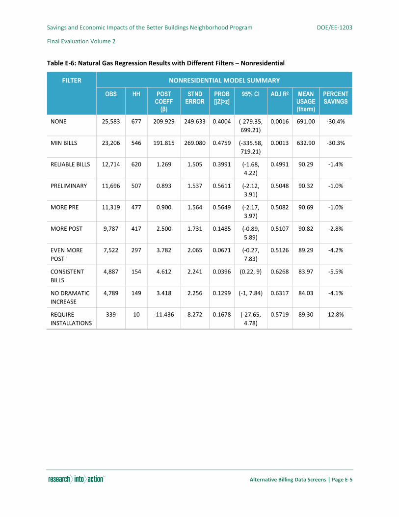
Savings and Economic Impacts of the Better Buildings Neighborhood Program DOE/EE-1203
Final Evaluation Volume 2
Alternative Billing Data Screens | Page E-5
Table E-6: Natural Gas Regression Results with Different Filters – Nonresidential
FILTER NONRESIDENTIAL MODEL SUMMARY
OBS HH POST COEFF (β)
STND ERROR
PROB [|Z|>z]
95% CI ADJ R2 MEAN USAGE (therm)
PERCENT SAVINGS
NONE 25,583 677 209.929 249.633 0.4004 (-279.35,
699.21)
0.0016 691.00 -30.4%
MIN BILLS 23,206 546 191.815 269.080 0.4759 (-335.58,
719.21)
0.0013 632.90 -30.3%
RELIABLE BILLS 12,714 620 1.269 1.505 0.3991 (-1.68,
4.22)
0.4991 90.29 -1.4%
PRELIMINARY 11,696 507 0.893 1.537 0.5611 (-2.12,
3.91)
0.5048 90.32 -1.0%
MORE PRE 11,319 477 0.900 1.564 0.5649 (-2.17,
3.97)
0.5082 90.69 -1.0%
MORE POST 9,787 417 2.500 1.731 0.1485 (-0.89,
5.89)
0.5107 90.82 -2.8%
EVEN MORE
POST
7,522 297 3.782 2.065 0.0671 (-0.27,
7.83)
0.5126 89.29 -4.2%
CONSISTENT
BILLS
4,887 154 4.612 2.241 0.0396 (0.22, 9) 0.6268 83.97 -5.5%
NO DRAMATIC
INCREASE
4,789 149 3.418 2.256 0.1299 (-1, 7.84) 0.6317 84.03 -4.1%
REQUIRE
INSTALLATIONS
339 10 -11.436 8.272 0.1678 (-27.65,
4.78)
0.5719 89.30 12.8%

Savings and Economic Impacts of the Better Buildings Neighborhood Program DOE/EE-1203
Final Evaluation Volume 2
Fuel Prices | Page F-1
APPENDIX F. FUEL PRICES
Table F-1: Commercial Energy Prices
STATE ELECTRICITY (KWH)* NATURAL GAS (THERM)**
Colorado $ 0.09 $ 0.80
Georgia $ 0.10 $ 1.06
Massachusetts $ 0.14 $ 1.11
Michigan $ 0.10 $ 0.92
North Carolina $ 0.08 $ 0.96
New Hampshire $ 0.14 $ 1.19
Ohio $ 0.10 $ 0.81
Texas $ 0.09 $ 0.71
Virginia $ 0.08 $ 0.96
Washington $ 0.07 $ 1.04
* 2011 average price per kWh: http://www.eia.gov/electricity/sales_revenue_price/pdf/table5_b.pdf.
** Average Price per therm from January 2011 through June 2012: http://www.eia.gov/dnav/ng/ng_pri_sum_dcu_nus_m.htm.
Table F-2: Residential Energy Prices
STATE ELECTRICITY
(KWH) *
NATURAL GAS
(THERM) **
FUEL OIL – TYPE 2
(GALLON) ***
PROPANE/LPG
(GALLON) ***
Alabama $ 0.11 $ 1.75 $ 3.80 $ 2.65
Arizona $ 0.11 $ 1.71 $ 3.80 $ 2.65
California $ 0.15 $ 0.98 $ 3.80 $ 2.65
Colorado $ 0.11 $ 0.97 $ 3.80 $ 2.65
Connecticut $ 0.18 $ 1.53 $ 3.80 $ 2.65
Florida $ 0.12 $ 1.92 $ 3.80 $ 2.65
Georgia $ 0.11 $ 1.90 $ 3.80 $ 2.65
Illinois $ 0.12 $ 1.02 $ 3.80 $ 2.65
Indiana $ 0.10 $ 1.12 $ 3.80 $ 2.65
Massachusetts $ 0.15 $ 1.38 $ 3.80 $ 2.65
Maine $ 0.15 $ 1.50 $ 3.80 $ 2.65
Continued…
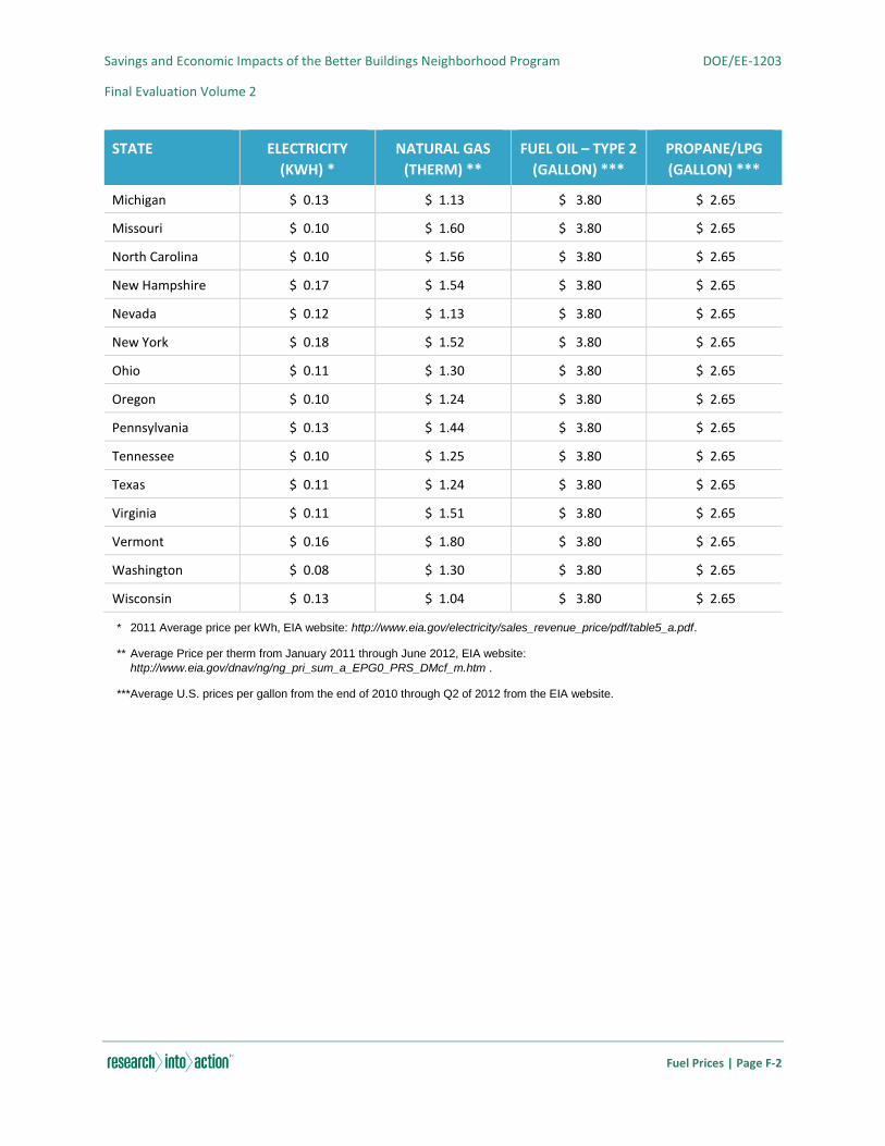
Savings and Economic Impacts of the Better Buildings Neighborhood Program DOE/EE-1203
Final Evaluation Volume 2
Fuel Prices | Page F-2
STATE ELECTRICITY
(KWH) *
NATURAL GAS
(THERM) **
FUEL OIL – TYPE 2
(GALLON) ***
PROPANE/LPG
(GALLON) ***
Michigan $ 0.13 $ 1.13 $ 3.80 $ 2.65
Missouri $ 0.10 $ 1.60 $ 3.80 $ 2.65
North Carolina $ 0.10 $ 1.56 $ 3.80 $ 2.65
New Hampshire $ 0.17 $ 1.54 $ 3.80 $ 2.65
Nevada $ 0.12 $ 1.13 $ 3.80 $ 2.65
New York $ 0.18 $ 1.52 $ 3.80 $ 2.65
Ohio $ 0.11 $ 1.30 $ 3.80 $ 2.65
Oregon $ 0.10 $ 1.24 $ 3.80 $ 2.65
Pennsylvania $ 0.13 $ 1.44 $ 3.80 $ 2.65
Tennessee $ 0.10 $ 1.25 $ 3.80 $ 2.65
Texas $ 0.11 $ 1.24 $ 3.80 $ 2.65
Virginia $ 0.11 $ 1.51 $ 3.80 $ 2.65
Vermont $ 0.16 $ 1.80 $ 3.80 $ 2.65
Washington $ 0.08 $ 1.30 $ 3.80 $ 2.65
Wisconsin $ 0.13 $ 1.04 $ 3.80 $ 2.65
* 2011 Average price per kWh, EIA website: http://www.eia.gov/electricity/sales_revenue_price/pdf/table5_a.pdf.
** Average Price per therm from January 2011 through June 2012, EIA website:
http://www.eia.gov/dnav/ng/ng_pri_sum_a_EPG0_PRS_DMcf_m.htm .
***Average U.S. prices per gallon from the end of 2010 through Q2 of 2012 from the EIA website.
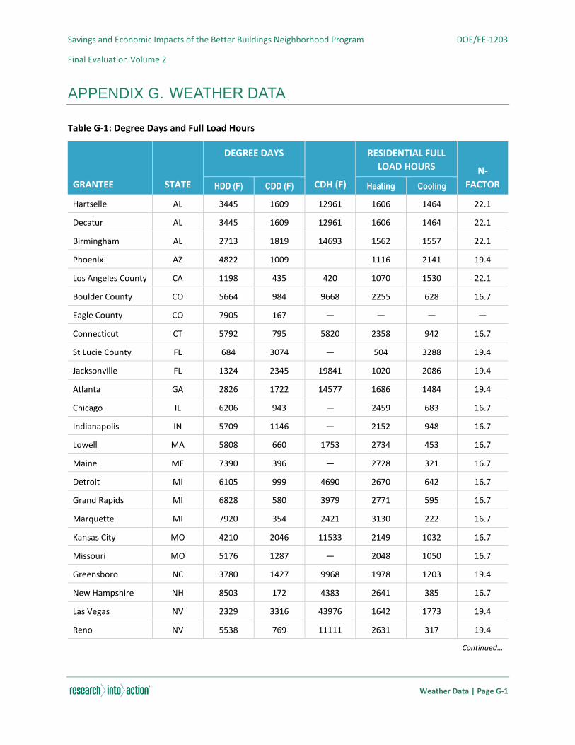
Savings and Economic Impacts of the Better Buildings Neighborhood Program DOE/EE-1203
Final Evaluation Volume 2
Weather Data | Page G-1
APPENDIX G. WEATHER DATA
Table G-1: Degree Days and Full Load Hours
GRANTEE STATE
DEGREE DAYS
CDH (F)
RESIDENTIAL FULL
LOAD HOURS N-
FACTOR HDD (F) CDD (F) Heating Cooling
Hartselle AL 3445 1609 12961 1606 1464 22.1
Decatur AL 3445 1609 12961 1606 1464 22.1
Birmingham AL 2713 1819 14693 1562 1557 22.1
Phoenix AZ 4822 1009 1116 2141 19.4
Los Angeles County CA 1198 435 420 1070 1530 22.1
Boulder County CO 5664 984 9668 2255 628 16.7
Eagle County CO 7905 167 — — — —
Connecticut CT 5792 795 5820 2358 942 16.7
St Lucie County FL 684 3074 — 504 3288 19.4
Jacksonville FL 1324 2345 19841 1020 2086 19.4
Atlanta GA 2826 1722 14577 1686 1484 19.4
Chicago IL 6206 943 — 2459 683 16.7
Indianapolis IN 5709 1146 — 2152 948 16.7
Lowell MA 5808 660 1753 2734 453 16.7
Maine ME 7390 396 — 2728 321 16.7
Detroit MI 6105 999 4690 2670 642 16.7
Grand Rapids MI 6828 580 3979 2771 595 16.7
Marquette MI 7920 354 2421 3130 222 16.7
Kansas City MO 4210 2046 11533 2149 1032 16.7
Missouri MO 5176 1287 — 2048 1050 16.7
Greensboro NC 3780 1427 9968 1978 1203 19.4
New Hampshire NH 8503 172 4383 2641 385 16.7
Las Vegas NV 2329 3316 43976 1642 1773 19.4
Reno NV 5538 769 11111 2631 317 19.4
Continued…
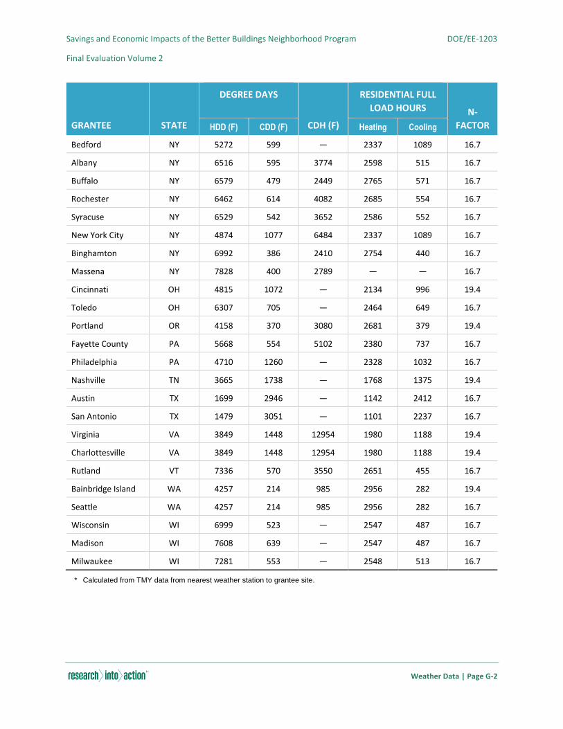
Savings and Economic Impacts of the Better Buildings Neighborhood Program DOE/EE-1203
Final Evaluation Volume 2
Weather Data | Page G-2
GRANTEE STATE
DEGREE DAYS
CDH (F)
RESIDENTIAL FULL
LOAD HOURS N-
FACTOR HDD (F) CDD (F) Heating Cooling
Bedford NY 5272 599 — 2337 1089 16.7
Albany NY 6516 595 3774 2598 515 16.7
Buffalo NY 6579 479 2449 2765 571 16.7
Rochester NY 6462 614 4082 2685 554 16.7
Syracuse NY 6529 542 3652 2586 552 16.7
New York City NY 4874 1077 6484 2337 1089 16.7
Binghamton NY 6992 386 2410 2754 440 16.7
Massena NY 7828 400 2789 — — 16.7
Cincinnati OH 4815 1072 — 2134 996 19.4
Toledo OH 6307 705 — 2464 649 16.7
Portland OR 4158 370 3080 2681 379 19.4
Fayette County PA 5668 554 5102 2380 737 16.7
Philadelphia PA 4710 1260 — 2328 1032 16.7
Nashville TN 3665 1738 — 1768 1375 19.4
Austin TX 1699 2946 — 1142 2412 16.7
San Antonio TX 1479 3051 — 1101 2237 16.7
Virginia VA 3849 1448 12954 1980 1188 19.4
Charlottesville VA 3849 1448 12954 1980 1188 19.4
Rutland VT 7336 570 3550 2651 455 16.7
Bainbridge Island WA 4257 214 985 2956 282 19.4
Seattle WA 4257 214 985 2956 282 16.7
Wisconsin WI 6999 523 — 2547 487 16.7
Madison WI 7608 639 — 2547 487 16.7
Milwaukee WI 7281 553 — 2548 513 16.7
* Calculated from TMY data from nearest weather station to grantee site.
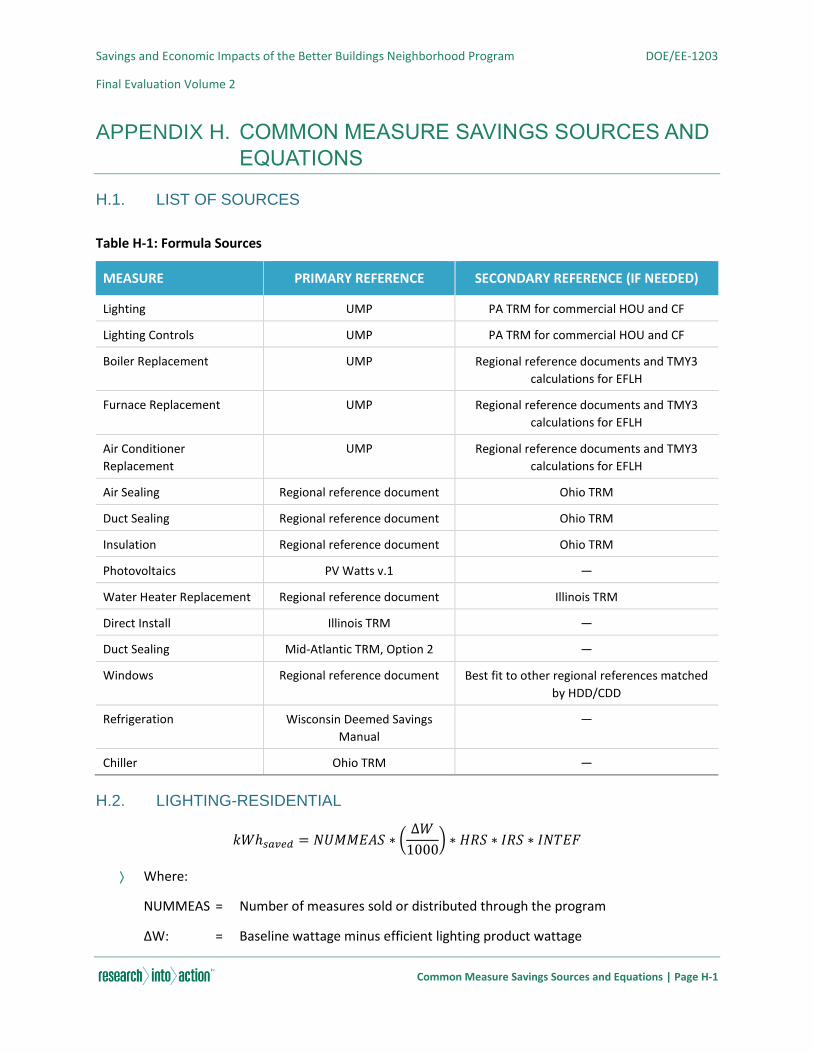
Savings and Economic Impacts of the Better Buildings Neighborhood Program DOE/EE-1203
Final Evaluation Volume 2
Common Measure Savings Sources and Equations | Page H-1
APPENDIX H. COMMON MEASURE SAVINGS SOURCES AND
EQUATIONS
H.1. LIST OF SOURCES
Table H-1: Formula Sources
MEASURE PRIMARY REFERENCE SECONDARY REFERENCE (IF NEEDED)
Lighting UMP PA TRM for commercial HOU and CF
Lighting Controls UMP PA TRM for commercial HOU and CF
Boiler Replacement UMP Regional reference documents and TMY3
calculations for EFLH
Furnace Replacement UMP Regional reference documents and TMY3
calculations for EFLH
Air Conditioner
Replacement
UMP Regional reference documents and TMY3
calculations for EFLH
Air Sealing Regional reference document Ohio TRM
Duct Sealing Regional reference document Ohio TRM
Insulation Regional reference document Ohio TRM
Photovoltaics PV Watts v.1 —
Water Heater Replacement Regional reference document Illinois TRM
Direct Install Illinois TRM —
Duct Sealing Mid-Atlantic TRM, Option 2 —
Windows Regional reference document Best fit to other regional references matched
by HDD/CDD
Refrigeration Wisconsin Deemed Savings
Manual
—
Chiller Ohio TRM —
H.2. LIGHTING-RESIDENTIAL
𝑘𝑊ℎ𝑠𝑎𝑣𝑒𝑑 = 𝑁𝑈𝑀𝑀𝐸𝐴𝑆 ∗ (∆𝑊
1000) ∗ 𝐻𝑅𝑆 ∗ 𝐼𝑅𝑆 ∗ 𝐼𝑁𝑇𝐸𝐹
Where:
NUMMEAS = Number of measures sold or distributed through the program
ΔW: = Baseline wattage minus efficient lighting product wattage
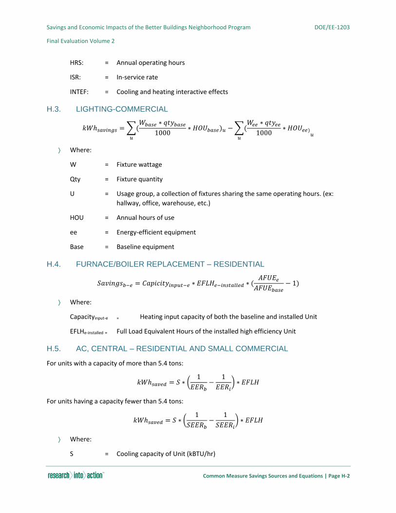
Savings and Economic Impacts of the Better Buildings Neighborhood Program DOE/EE-1203
Final Evaluation Volume 2
Common Measure Savings Sources and Equations | Page H-2
HRS: = Annual operating hours
ISR: = In-service rate
INTEF: = Cooling and heating interactive effects
H.3. LIGHTING-COMMERCIAL
𝑘𝑊ℎ𝑠𝑎𝑣𝑖𝑛𝑔𝑠 = ∑(𝑊𝑏𝑎𝑠𝑒 ∗ 𝑞𝑡𝑦𝑏𝑎𝑠𝑒
1000∗ 𝐻𝑂𝑈𝑏𝑎𝑠𝑒)𝑢
𝑢
− ∑(𝑊𝑒𝑒 ∗ 𝑞𝑡𝑦𝑒𝑒
1000∗ 𝐻𝑂𝑈𝑒𝑒)
𝑢𝑢
Where:
W = Fixture wattage
Qty = Fixture quantity
U = Usage group, a collection of fixtures sharing the same operating hours. (ex:
hallway, office, warehouse, etc.)
HOU = Annual hours of use
ee = Energy-efficient equipment
Base = Baseline equipment
H.4. FURNACE/BOILER REPLACEMENT – RESIDENTIAL
𝑆𝑎𝑣𝑖𝑛𝑔𝑠𝑏−𝑒 = 𝐶𝑎𝑝𝑖𝑐𝑖𝑡𝑦𝑖𝑛𝑝𝑢𝑡−𝑒 ∗ 𝐸𝐹𝐿𝐻𝑒−𝑖𝑛𝑠𝑡𝑎𝑙𝑙𝑒𝑑 ∗ (𝐴𝐹𝑈𝐸𝑒
𝐴𝐹𝑈𝐸𝑏𝑎𝑠𝑒− 1)
Where:
Capacityinput-e = Heating input capacity of both the baseline and installed Unit
EFLHe-installed = Full Load Equivalent Hours of the installed high efficiency Unit
H.5. AC, CENTRAL – RESIDENTIAL AND SMALL COMMERCIAL
For units with a capacity of more than 5.4 tons:
𝑘𝑊ℎ𝑠𝑎𝑣𝑒𝑑 = 𝑆 ∗ (1
𝐸𝐸𝑅𝑏−
1
𝐸𝐸𝑅𝑖) ∗ 𝐸𝐹𝐿𝐻
For units having a capacity fewer than 5.4 tons:
𝑘𝑊ℎ𝑠𝑎𝑣𝑒𝑑 = 𝑆 ∗ (1
𝑆𝐸𝐸𝑅𝑏−
1
𝑆𝐸𝐸𝑅𝑖) ∗ 𝐸𝐹𝐿𝐻
Where:
S = Cooling capacity of Unit (kBTU/hr)
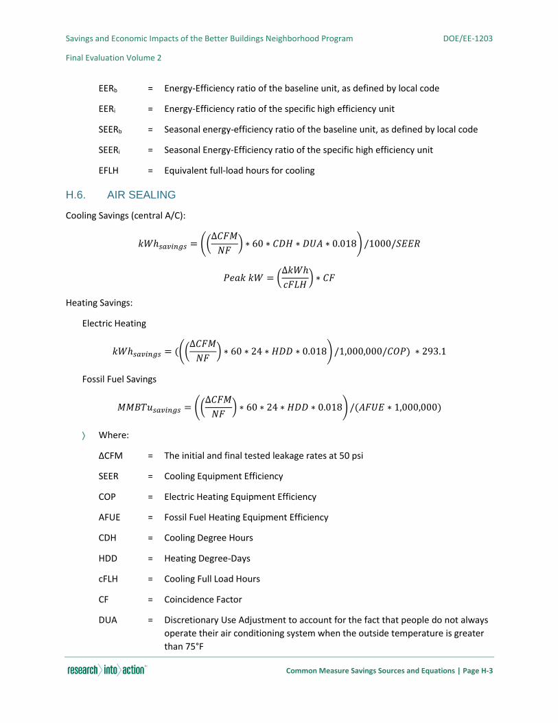
Savings and Economic Impacts of the Better Buildings Neighborhood Program DOE/EE-1203
Final Evaluation Volume 2
Common Measure Savings Sources and Equations | Page H-3
EERb = Energy-Efficiency ratio of the baseline unit, as defined by local code
EERi = Energy-Efficiency ratio of the specific high efficiency unit
SEERb = Seasonal energy-efficiency ratio of the baseline unit, as defined by local code
SEERi = Seasonal Energy-Efficiency ratio of the specific high efficiency unit
EFLH = Equivalent full-load hours for cooling
H.6. AIR SEALING
Cooling Savings (central A/C):
𝑘𝑊ℎ𝑠𝑎𝑣𝑖𝑛𝑔𝑠 = ((∆𝐶𝐹𝑀
𝑁𝐹) ∗ 60 ∗ 𝐶𝐷𝐻 ∗ 𝐷𝑈𝐴 ∗ 0.018) /1000/𝑆𝐸𝐸𝑅
𝑃𝑒𝑎𝑘 𝑘𝑊 = (∆𝑘𝑊ℎ
𝑐𝐹𝐿𝐻) ∗ 𝐶𝐹
Heating Savings:
Electric Heating
𝑘𝑊ℎ𝑠𝑎𝑣𝑖𝑛𝑔𝑠 = (((∆𝐶𝐹𝑀
𝑁𝐹) ∗ 60 ∗ 24 ∗ 𝐻𝐷𝐷 ∗ 0.018) /1,000,000/𝐶𝑂𝑃) ∗ 293.1
Fossil Fuel Savings
𝑀𝑀𝐵𝑇𝑢𝑠𝑎𝑣𝑖𝑛𝑔𝑠 = ((∆𝐶𝐹𝑀
𝑁𝐹) ∗ 60 ∗ 24 ∗ 𝐻𝐷𝐷 ∗ 0.018) /(𝐴𝐹𝑈𝐸 ∗ 1,000,000)
Where:
ΔCFM = The initial and final tested leakage rates at 50 psi
SEER = Cooling Equipment Efficiency
COP = Electric Heating Equipment Efficiency
AFUE = Fossil Fuel Heating Equipment Efficiency
CDH = Cooling Degree Hours
HDD = Heating Degree-Days
cFLH = Cooling Full Load Hours
CF = Coincidence Factor
DUA = Discretionary Use Adjustment to account for the fact that people do not always
operate their air conditioning system when the outside temperature is greater
than 75°F
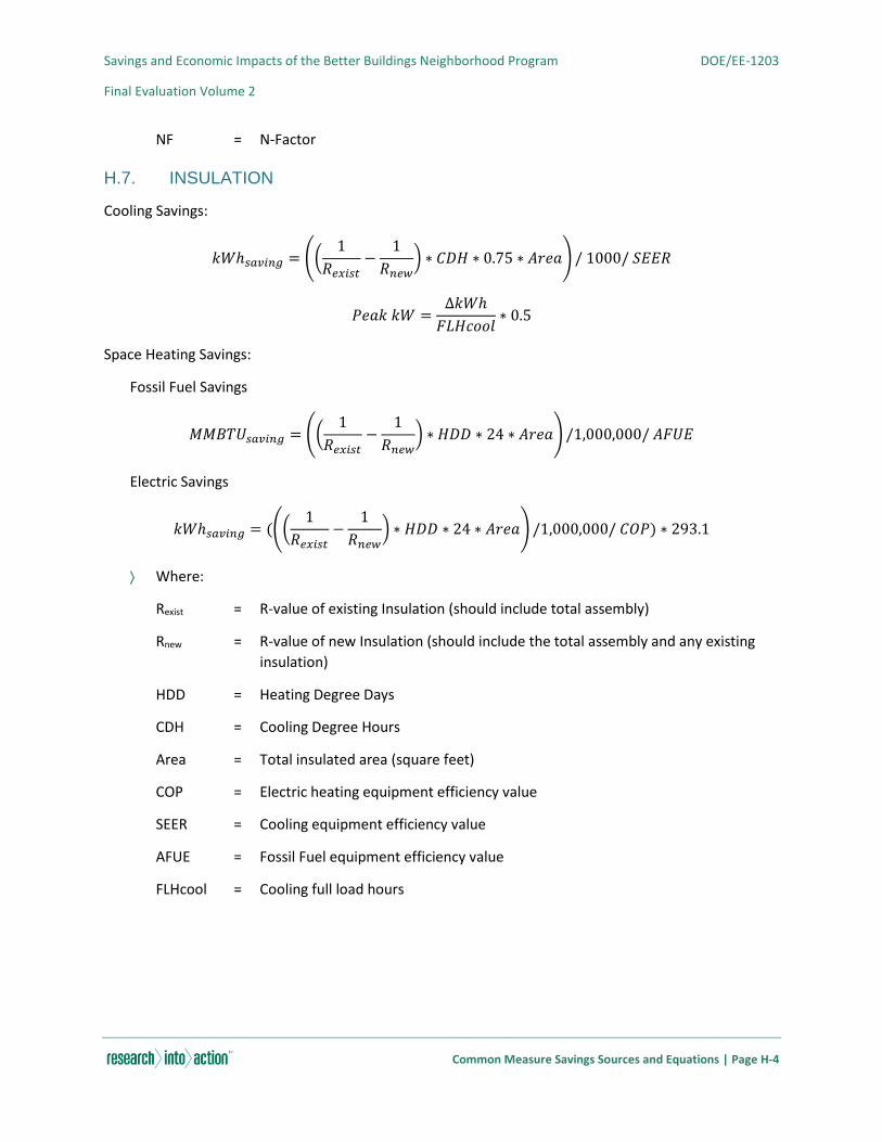
Savings and Economic Impacts of the Better Buildings Neighborhood Program DOE/EE-1203
Final Evaluation Volume 2
Common Measure Savings Sources and Equations | Page H-4
NF = N-Factor
H.7. INSULATION
Cooling Savings:
𝑘𝑊ℎ𝑠𝑎𝑣𝑖𝑛𝑔 = ((1
𝑅𝑒𝑥𝑖𝑠𝑡−
1
𝑅𝑛𝑒𝑤) ∗ 𝐶𝐷𝐻 ∗ 0.75 ∗ 𝐴𝑟𝑒𝑎) / 1000/ 𝑆𝐸𝐸𝑅
𝑃𝑒𝑎𝑘 𝑘𝑊 =∆𝑘𝑊ℎ
𝐹𝐿𝐻𝑐𝑜𝑜𝑙∗ 0.5
Space Heating Savings:
Fossil Fuel Savings
𝑀𝑀𝐵𝑇𝑈𝑠𝑎𝑣𝑖𝑛𝑔 = ((1
𝑅𝑒𝑥𝑖𝑠𝑡−
1
𝑅𝑛𝑒𝑤) ∗ 𝐻𝐷𝐷 ∗ 24 ∗ 𝐴𝑟𝑒𝑎) /1,000,000/ 𝐴𝐹𝑈𝐸
Electric Savings
𝑘𝑊ℎ𝑠𝑎𝑣𝑖𝑛𝑔 = (((1
𝑅𝑒𝑥𝑖𝑠𝑡−
1
𝑅𝑛𝑒𝑤) ∗ 𝐻𝐷𝐷 ∗ 24 ∗ 𝐴𝑟𝑒𝑎) /1,000,000/ 𝐶𝑂𝑃) ∗ 293.1
Where:
Rexist = R-value of existing Insulation (should include total assembly)
Rnew = R-value of new Insulation (should include the total assembly and any existing
insulation)
HDD = Heating Degree Days
CDH = Cooling Degree Hours
Area = Total insulated area (square feet)
COP = Electric heating equipment efficiency value
SEER = Cooling equipment efficiency value
AFUE = Fossil Fuel equipment efficiency value
FLHcool = Cooling full load hours
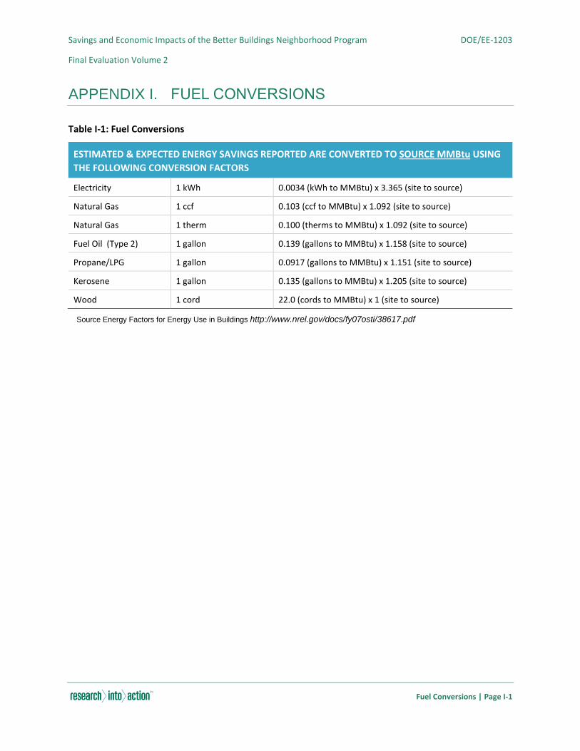
Savings and Economic Impacts of the Better Buildings Neighborhood Program DOE/EE-1203
Final Evaluation Volume 2
Fuel Conversions | Page I-1
APPENDIX I. FUEL CONVERSIONS
Table I-1: Fuel Conversions
ESTIMATED & EXPECTED ENERGY SAVINGS REPORTED ARE CONVERTED TO SOURCE MMBtu USING
THE FOLLOWING CONVERSION FACTORS
Electricity 1 kWh 0.0034 (kWh to MMBtu) x 3.365 (site to source)
Natural Gas 1 ccf 0.103 (ccf to MMBtu) x 1.092 (site to source)
Natural Gas 1 therm 0.100 (therms to MMBtu) x 1.092 (site to source)
Fuel Oil (Type 2) 1 gallon 0.139 (gallons to MMBtu) x 1.158 (site to source)
Propane/LPG 1 gallon 0.0917 (gallons to MMBtu) x 1.151 (site to source)
Kerosene 1 gallon 0.135 (gallons to MMBtu) x 1.205 (site to source)
Wood 1 cord 22.0 (cords to MMBtu) x 1 (site to source)
Source Energy Factors for Energy Use in Buildings http://www.nrel.gov/docs/fy07osti/38617.pdf

Savings and Economic Impacts of the Better Buildings Neighborhood Program DOE/EE-1203
Final Evaluation Volume 2
Residential and Commercial Verification Surveys | Page J-1
APPENDIX J. RESIDENTIAL AND COMMERCIAL
VERIFICATION SURVEYS
J.1. RESIDENTIAL PARTICIPANT: BETTER BUILDINGS NEIGHBORHOOD
PROGRAMS TELEPHONE SURVEY
J.1.1. GENERAL INFORMATION (FROM GRANTEE DOCUMENTATION)
Participant Name: Grantee Name:
Project Ref
Number:
Project
Completion
Date:
Contact Address: City:
State: Zip:
Electric Utility: Nat. Gas Utility
Other Fuel Source: Nexant Caller:
Date: Time:
Notes:
J.1.2. PROJECT MEASURE INFORMATION (FROM GRANTEE DOCUMENTATION) Circle all that apply
Weatherization
Measures:
Air/Duct Sealing, Insulation, Doors, Windows, Programmable Thermostat
Appliance Measures: Water Heater, Furnace, Boiler, Air Conditioner, Evaporative Cooler, Heat
Pump, Refrigerator, Freezer, Dishwasher, Clothes Washer
Lighting Measures: CFLs, Linear Fluorescents, LEDs
Renewable Energy Solar Photovoltaic, Solar Thermal
Other Measures: List:

Savings and Economic Impacts of the Better Buildings Neighborhood Program DOE/EE-1203
Final Evaluation Volume 2
Residential and Commercial Verification Surveys | Page J-2
Hello, my name is <Your Name> from Nexant and I’m calling on behalf of the < Name of
grantee/subgrantee and umbrella program > and the U.S. Department of Energy. We are conducting a
national level study to assess the energy savings associated with program participants who implemented
energy upgrade projects. May I please speak with <Contact Name>?
IF CONTACT NOT AVAILABLE, LEAVE MESSAGE: I am calling because as a participant in <Name of
grantee/subgrantee and umbrella program>, we would like your feedback as part of a short survey. Your
responses will contribute to the national study of the Better Building Neighborhood Program (BBNP),
which is the Department of Energy’s (DOE) program that funded <Name of grantee/subgrantee and
umbrella program>. We would greatly appreciate your participation in this voluntary survey. Please give
me a call back at your earliest convenience so that we can complete a short telephone survey. <Give
Contact Information including Phone Number>
IF CONTACT NOT AVAILABLE, LEAVE MESSAGE WITH SOMEONE ELSE: I am calling because as a
participant in <Name of grantee/subgrantee and umbrella program>, we would like your feedback as
part of a short survey. Your responses will contribute to the national study of the Better Building
Neighborhood Program (BBNP), which is the Department of Energy’s (DOE) program that funded <Name
of grantee/subgrantee and umbrella program>. Are you familiar with this program and the energy
upgrades completed at your house?
a) [If no]: Would you please have <Contact Name> call me back at their earliest convenience so
that we can set up a time to speak? My phone number is <Your Phone Number>.
b) [If yes]: Would you be willing to participate in this voluntary survey? Your feedback will not
affect your incentive and is simply used to learn how DOE may improve future programs. All
information provided will remain private to the extent permitted by law
i. [If yes] Thank you! Knowing that this is voluntary, we appreciate that you are willing
to be interviewed. If you have any additional questions regarding this study, please
contact Kevin Afflerbaugh, Project Manager at Nexant at 303-998-2462 or Dr.
Edward Vine at the Lawrence Berkeley National Laboratory (LBNL) at 510-486-6047.
ii. [If no]: Would you please have <Contact Name> call me back at their earliest
convenience so that we can set up a time to speak? My phone number is <Your
Phone Number>.
IF CONTACT NO LONGER AT SITE: [Questions will not apply, thank the person for their time and move on
to the next participant]
AFTER LOCATING PROPER CONTACT:
I am calling because as a participant in <Name of grantee/subgrantee and umbrella program>, we would
like your feedback as part of a short survey. This survey will be used to verify information regarding your
project funded by DOE. Your responses will contribute to the national study of the Better Building
Neighborhood Program (BBNP), which is the Department of Energy’s (DOE) program that funded <Name
of grantee/subgrantee and umbrella program>. We would greatly appreciate your participation in this

Savings and Economic Impacts of the Better Buildings Neighborhood Program DOE/EE-1203
Final Evaluation Volume 2
Residential and Commercial Verification Surveys | Page J-3
voluntary survey. Your feedback will not affect your incentive and is simply used to learn how DOE may
improve future programs. All information provided will remain private to the extent permitted by law.
Could I ask you a few questions about the measures you installed through the program? This will take
approximately 10 minutes.
a) [If yes] Thank you! Knowing that this is voluntary, we appreciate that you are willing to be
interviewed. If you have any additional questions regarding this study, please contact Kevin
Afflerbaugh, Project Manager at Nexant at 303-998-2462 or Dr. Edward Vine at the
Lawrence Berkeley National Laboratory at 510-486-6047.
b) [If no] [If they don’t agree, ask them if there is another time that would be more convenient
for them. If they still say no, thank them for their time, and move on.]
IF PARTICIPANT IS FROM A GRANTEE SELECTED FOR ONSITE VISITS:
As an additional part of the study, we also will be conducting onsite visits at a selection of project sites.
These onsite visits last an average of thirty minutes, and a trained professional engineer will conduct a
walk-through of your residence to gather additional information on the measures you installed. As an
incentive for allowing us to conduct an onsite visit, we will provide a $50 Visa gift card at the completion
of the site visit. Would you be willing to let one of our engineers come to your home for this purpose?
a) [If yes] Excellent! Before we start the survey, let’s schedule the visit. We are currently
scheduling visits the week of <insert week>. [Let’s give them a few times to work with.]
[Record Scheduled Time & Date:] _________________________________
Again, the visit will take approximately ½ hour. We will need access to the areas of your house where
you had the work done. The field engineer will provide you with proper identification from Nexant upon
arrival. Who will be the contact for this visit?___________________
Is there anything the engineer needs to be aware of before arriving at your home? [Prompt examples if
necessary: Dogs, security code for neighborhood entry, etc.]
_________________________________________________
If you need to reschedule or cancel, please contact ______ at ____________
b) [If no] That’s fine. Let’s get started with the survey.
>>> start the survey<<<<
General Energy Upgrade Questions
1. I would now like to verify what energy upgrade measures you had installed. According to program
records you had the following measures installed: <describe measures from project information>. Is
this correct?
2. [If no] What was actually installed? ___________________[Be sure to ask survey questions
appropriate for the measures actually installed]

Savings and Economic Impacts of the Better Buildings Neighborhood Program DOE/EE-1203
Final Evaluation Volume 2
Residential and Commercial Verification Surveys | Page J-4
General Information Now I am going to ask a few questions regarding your home.
3. What year was your home built?_____________
4. What is the total conditioned square footage of your home? ______________
5. How many people live in your home? ______ Has there been any change to that number in the last 3
years? ______
6. How many bedrooms? ________
7. How many bathrooms? _______
8. Have there been any modifications to your home in the last 3 years? If so, please
describe._______________________________________________________
Heating System Info
The next few questions will focus on your heating system.
9. What is your primary heating fuel--------------------------- Natural Gas
Electricity
Propane
Fuel Oil
Kerosene
Wood
Geothermal
Other:
10. What is your primary heat system type:------------------- Gas Furnace
Electric Furnace
Wood Stove
Gas Stove
Ground Source Heat Pump
Air Source Heat Pump
Space Heater
Gas boiler--Baseboard

Savings and Economic Impacts of the Better Buildings Neighborhood Program DOE/EE-1203
Final Evaluation Volume 2
Residential and Commercial Verification Surveys | Page J-5
Gas boiler—Radiant
Gas boiler – other
Baseboard--Electric
Radiant--Electric
Other:
If participant did not receive a new heating system (furnace/boiler/etc.) as part of the energy upgrade,
ask questions 11-15. Otherwise skip to Question 16. If they received a new heating system, this
information will be gathered in the appropriate section detailing their new heating system.
Can you please verify the age, make, model number, and size of the new furnace? This information is
often located on a label on the frame of the furnace. (Make sure they know they may have to take off
the panel where all this info is located.)
11. Age of primary heat system:____________
12. Primary heat system make:_____________
13. Primary heat system model:____________
14. Efficiency (AFUE): _______________
15. Size (btuh): In_______Out_______ (the unit might only list one)
16. Do you have a secondary heating system? (Yes/No) [If no, skip to question 21]
17. Secondary Heat System Type:---------------------- Fireplace (wood/gas)
Gas Furnace
Electric Furnace
Wood Stove
Gas Stove
Ground Source Heat Pump
Air Source Heat Pump
Space Heater
Gas boiler
Baseboard (electric/hydronic)
Radiant (electric/hydronic)

Savings and Economic Impacts of the Better Buildings Neighborhood Program DOE/EE-1203
Final Evaluation Volume 2
Residential and Commercial Verification Surveys | Page J-6
Other:
18. Age of secondary heat system? ________
19. Approximately how often is secondary heat source used? _________
20. Approximately how much square footage is heated by secondary heat source? ________
21. What type of thermostat do you use? (Programmable / non-programmable)
22. Approximate heating-season thermostat settings:
Weekday
Daytime
Weekday
evening
Weekday
Overnight
Weekend
Daytime
Weekend
evening
Weekend
overnight
Cooling System 23. Do you currently have a cooling system? (that is, central air, room air conditioning, evaporative
cooler) [If no, skip to first section with applicable measure installed by participant that requires
verification.]
24. Primary Cooling System Type:------------------------------ Central Air Conditioner
Window Air Conditioner
Evaporative cooler
Air Source Heat Pump
Ground Source Heat
Pump
Other:
If participant did not receive a new cooling system as part of their energy upgrade (air conditioner/evap
cooler/etc), ask questions 25 – 29. Otherwise skip to Question 30. If they received a new cooling system,
this information will be gathered in the appropriate section detailing their new cooling system.
25. What is the approximate age of the primary cooling unit? ________
Can you please verify the make, model number, capacity, and efficiency of the cooling system? This
information is often located on a label on the side of the air conditioner
26. Primary cooling unit make? _________
27. Primary cooling unit model: _________
28. Primary cooling unit tonnage: __________

Savings and Economic Impacts of the Better Buildings Neighborhood Program DOE/EE-1203
Final Evaluation Volume 2
Residential and Commercial Verification Surveys | Page J-7
29. Primary cooling unit SEER/CFM: ___________
30. In addition to your primary cooling system, do you have any additional cooling systems? [If no,
skip to question 35]
31. Secondary Cooling System Type (if applicable): ------ Central Air Conditioner
Window Air Conditioner
Evaporative Cooler
Air Source Heat Pump
Ground Source Heat Pump
Other:
32. Age of secondary cooling system: ______
33. Approximately how often is secondary cooling system used? ________
34. Approximately how much square footage is cooled by secondary cooling system? _______
35. Approximate cooling-season thermostat settings:
Weekday
Daytime
Weekday
evening
Weekday
Overnight
Weekend
Daytime
Weekend
evening
Weekend
overnight
Weatherization Measures
Insulation
Wall Insulation 36. What is the total area (sq. ft.) of the walls that were insulated? __________
37. Type of insulation prior to upgrade ---------------- None
Rigid Foam
Blanket Batts
Vermiculite
Rockwool
Fiberglass
Cellulose Fiber
38. Approximate inches of wall insulation that existed prior to the upgrade ________
39. Value prior to upgrade (if known): ___________

Savings and Economic Impacts of the Better Buildings Neighborhood Program DOE/EE-1203
Final Evaluation Volume 2
Residential and Commercial Verification Surveys | Page J-8
40. Type of insulation added ----------------------------- None
Rigid Foam
Blanket Batts
Vermiculite
Rockwool
Fiberglass
Cellulose Fiber
41. How many inches of insulation were added? _____________
42. Retrofit R-Value (if known): ______________
Attic Insulation 43. What is the area of the attic floor that was insulated (sq. ft.):
44. Type of insulation prior to upgrade ------------------------ None
Rigid Foam
Blanket Batts
Vermiculite
Rockwool
Fiberglass
Cellulose Fiber
45. Inches of attic insulation prior to upgrade: ___________
46. R-Value prior to upgrade (if known): _____________
47. Type of insulation added ---------------------------------- None
Rigid Foam
Blanket Batts
Vermiculite
Rockwool
Fiberglass
Cellulose Fiber
48. How many inches were added? ____________
49. Retrofit R-Value (if known): ________________
Crawl Space Insulation 50. What is the total area (sq. ft.) of the crawl space wall, floor, and
ceiling that were insulated? _________________

Savings and Economic Impacts of the Better Buildings Neighborhood Program DOE/EE-1203
Final Evaluation Volume 2
Residential and Commercial Verification Surveys | Page J-9
51. Type of insulation prior to upgrade ------------------------------ None
Rigid Foam
Blanket Batts
Vermiculite
Rockwool
Fiberglass
Cellulose Fiber
52. Inches of crawl space insulation prior to upgrade: ______________
53. R-Value prior to upgrade (if known): ________________
54. Type of insulation added ------------------------------------------ None
Rigid Foam
Blanket Batts
Vermiculite
Rockwool
Fiberglass
Cellulose Fiber
55. How many inches were added? _______________
56. Retrofit R-Value (if known): _____________
Rim Joist Insulation 57. What is the total sq. ft. of rim joists insulated? _________
58. Type of insulation prior to upgrade ---------------------- None
Rigid Foam
Blanket Batts
Vermiculite
Rockwool
Fiberglass
Cellulose Fiber
59. Inches of rim joist insulation prior to upgrade: _________
60. R-Value prior to upgrade (if known): ______________
61. Type of insulation added --------------------------------- None
Rigid Foam
Blanket Batts
Vermiculite
Rockwool
Fiberglass
Cellulose Fiber

Savings and Economic Impacts of the Better Buildings Neighborhood Program DOE/EE-1203
Final Evaluation Volume 2
Residential and Commercial Verification Surveys | Page J-10
62. How many inches were added? ______________
63. Retrofit R-Value (if known): ________________
Windows
64. Energy ratings of each new type of window installed:
Type 1
U Factor:______
Solar Heat Gain Coefficient: _____
Type 2 (if applicable)
U Factor:______
Solar Heat Gain Coefficient: _____
Type 3 (if applicable)
U Factor:______
Solar Heat Gain Coefficient: _____
65. Quantity of each type of new window installed:
Type 1: _____Type 2:________Type 3:______
66. Total size in sq. ft. of each type of new window:
Type 1: _____Type 2:________Type 3:______
67. # of Panes: (single, dual, etc) Type 1: _____Type 2:________Type 3:______
68. What type of window was replaced?___________________________
69. How many panes did they have? ______________________________
70. What was the framing material?_______________________________
Doors
71. Quantity of new doors installed: _____________________
72. Size of each: _________________
73. Material of each (wood, glass, fiberglass, etc..): _________________

Savings and Economic Impacts of the Better Buildings Neighborhood Program DOE/EE-1203
Final Evaluation Volume 2
Residential and Commercial Verification Surveys | Page J-11
74. What were the old doors? _____________________
Duct and Air Sealing
75. What part of your home was sealed? (Ducts/Windows/Door/Attic)
76. Quantity of each item sealed? (feet of ducts/number of doors or
windows/sq. ft. of attic/crawlspace)
___________________________________________
77. What air sealing measures were performed for each area? (ex. Spray foam, caulk, mastic etc):
_____________________________________________
Programmable Thermostat We discussed your current set points earlier in this survey, now I would like to understand the settings
associated with your old thermostat.
78. With your previous thermostat, were the settings the same as the new thermostat?
79. [If no] What were the settings?
Summer
Weekday
Daytime
Weekday
evening
Weekday
Overnight
Weekend
Daytime
Weekend
evening
Weekend
overnight
Winter
Weekday
Daytime
Weekday
evening
Weekday
Overnight
Weekend
Daytime
Weekend
evening
Weekend
overnight
Appliance Measures
Water Heaters
80. What type of water heater did you purchase?------------------- Tankless
Storage
81. What is the fuel type? --------------------------------------------- Electric
Gas
Propane

Savings and Economic Impacts of the Better Buildings Neighborhood Program DOE/EE-1203
Final Evaluation Volume 2
Residential and Commercial Verification Surveys | Page J-12
Fuel Oil
Solar
82. Where is the water heater located?------------------------------- Garage
Basement
Closet
Laundry Room
83. Is the water heater in a conditioned space? ____________
84. Is the water heater wrapped with an insulating material? ________
85. Can you please verify the make, model number, capacity, and efficiency of the water heater?
This information is often located on a label on the frame of the water heater.
Make:_____________ Model:_________________
Capacity (gallons):_____________ Efficiency (Energy Factor 0 to 1): _______________
ENERGY STAR Label _______ R-Value of Tank ________
86. What was the temperature set point on your water heater prior to the retrofit? _______
87. What is the temperature set-point on your new water heater? ________________
88. What type of water heater did you replace? (Tankless / Storage)
89. Can you approximate its age? ______________
90. Was it the same fuel type as the new one? ___________
91. [If no] What was the fuel used by the old water heater? __________
92. Was it in good working condition when you replaced it? ___________
93. How did you dispose of the old water heater? (examples: sold / recycled / trashed / contractor
removed it)
Furnace 94. Can you please verify the make, model number, and input capacity of the new furnace? This
information is often located on a label on the frame of the furnace. (Make sure they know they will
likely have to take off the panel where all this info is located.)
Make:_____________ Model:_________________
Efficiency (AFUE): _______________

Savings and Economic Impacts of the Better Buildings Neighborhood Program DOE/EE-1203
Final Evaluation Volume 2
Residential and Commercial Verification Surveys | Page J-13
Size (btuh): In_______Out_______ (the unit might only list one)
95. What heating system type was replaced by the new furnace? (gas furnace, electric furnace, gas
boiler, etc)
96. How old was your previous heating system? _________
97. Was it in good working order when it was replaced? ______
98. What was the efficiency of your old furnace? ______
99. Why was it replaced? _____________________________________________________
100. How was it disposed of? (examples: sold / recycled / trashed)
101. Did the temperature set points on your programmable thermostat change after you installed
the new furnace? ______
102. [If yes] Please describe how they changed _______________________________
Boiler 103. Can you please verify the make, model number, and efficiency of the boiler? This information is
often located on a label on the frame of the boiler.
Make:_____________ Model:_________________
Efficiency (AFUE): _______________ Rated heating input (Btu/hr) _______
104. What heating system type was replaced by the new boiler? (examples: gas furnace, electric
furnace, gas boiler, etc)
105. How old was your previous heating system? _________
106. Was it in good working order when it was replaced? _______
107. What was the heat output (efficiency) rating of your old boiler? ______
108. Why was it replaced? _____________________________________________________
109. How was it disposed of? (examples: sold / recycled / trashed)
110. Did the temperature set points on your thermostat change after you installed the new boiler?
_______
111. [If yes] Please describe how they changed __________________________________
Central Air Conditioner 112. Can you please verify the make, model number, size and efficiency rating of the new air
conditioner? This information is often located on a label on the side of the air conditioner.
Make:_____________ Model:_________________
Tonnage: _______________ SEER: _____

Savings and Economic Impacts of the Better Buildings Neighborhood Program DOE/EE-1203
Final Evaluation Volume 2
Residential and Commercial Verification Surveys | Page J-14
113. Did you have a cooling system prior to the installation of your new air conditioner? ____ [If no,
this section is complete.]
114. What type of system? (examples: central air conditioner, evaporative cooler, window air
conditioner)
115. Was it in good working order when it was replaced? _______
116. How old was your previous cooling unit? _________
117. Why was it replaced? ______
118. How was it disposed of? (examples: sold / recycled / trashed)
119. What was the SEER rating of your old air conditioner? ______
120. Did you have the same thermostat with the old cooling system? _____________
121. Did the temperature set points on your thermostat change after you installed the new AC?
__________
122. [If yes] Please describe how they changed ____________________________________
Evaporative Cooler 123. Can you please verify the make, model number, size and efficiency of the new evaporative
cooler? This information is often located on a label on the frame of the cooler.
Make:_____________ Model:_________________
CFM: _____ Type: Whole house/Room
124. Did you have a cooling system prior to the installation of your new evaporative cooler?
_____________ [If no, this section is complete]
125. What type of system? (examples: central air conditioner, evaporative cooler, window air
conditioner)
126. Was it in good working order when it was replaced?___________
127. How old was your previous cooling unit? _________
128. Why was it replaced? _______________
129. How was it disposed of? (examples: sold / recycled / trashed)
130. What was the efficiency rating of the prior system (SEER or CFM)? __________
131. Did the temperature set points on your thermostat change after you installed the new cooler?
________
132. [If yes] Please describe how they changed _____________________________________

Savings and Economic Impacts of the Better Buildings Neighborhood Program DOE/EE-1203
Final Evaluation Volume 2
Residential and Commercial Verification Surveys | Page J-15
Heat Pump 133. Can you please verify the make, model number, and efficiency of the heat pump?
Make:_____________ Model:_________________
SEER: _______________ Heating Seasonal Performance Factor (HSPF): _______
Tonnage: ______
134. What type of heat pump was installed: Ground Source or Air Source
135. What is the heat pump used for: Heating/Cooling/Both
136. What heating/cooling system did this heat pump replace? (Gas furnace, central air conditioner,
lower efficiency heat pump, other)
137. How old was your previous heating/cooling unit? _________
138. Was it in good working order when it was replaced? _________
139. Why was it replaced? __________
140. How was it disposed of? (examples: sold / recycled / trashed)
141. Did the temperature set points on the thermostat change after you installed the new heat
pump? ______
142. [If yes] Please describe how they changed ____________________________________
Refrigerator 143. First, can you please verify the make and model number of the refrigerator? The model number
is often located on a label on the inside wall of the refrigerator.
Make _________________ Model _____________
144. What are the characteristics of your new refrigerator? [Circle applicable features below]
Appliance Characteristics
(Choose One in Each Applicable Category Below)
FRIDG: Configuration Top Freezer Side-by-Side Bottom
Freezer Single Door
Frost Type Frost-Free Manual
Through Door Features Water and/or
Ice None
Location Kitchen Garage Porch/Patio Basement Other:
_______

Savings and Economic Impacts of the Better Buildings Neighborhood Program DOE/EE-1203
Final Evaluation Volume 2
Residential and Commercial Verification Surveys | Page J-16
Air Conditioning in
room? Central AC Room AC None
Is the refrigerator
located in a heated
space?
Heated Unheated
145. How many cubic feet is the new refrigerator? __________
146. What was the approximate age of the refrigerator that was replaced? __________
147. Was it in good working order when you got rid of it? ______________
148. How did you dispose of it? (examples: sold/ recycled/ trashed/ did not get rid of it)
____________
149. If you still have it, where is it located? ___________
150. What is the make _____________and model ___________of the old refrigerator?
Freezer 151. First, can you please verify the brand and model number of the freezer? The model number is
often located on a label on the inside wall of the freezer.
Make______________ Model ______________
152. What type of freezer is it? (Upright/Chest)
153. How many cubic feet is the freezer? __________
154. Is the freezer located in an air conditioned room? __________
155. What was the approximate age of the freezer that you replaced? __________
156. Was it in good working order when you got rid of it? __________
157. How did you dispose of it? (examples: sold/ recycled/ trashed/did not get rid of it)
158. If you still have it where is it located? __________
159. What is the brand __________ and model __________?
Dishwasher 160. First, can you please verify the brand and model number of the dishwasher that you purchased?
The model number is often located on a label on the inside frame of the dishwasher just as you open
the door.
Make __________ Model __________
161. About how many loads per week do you run? __________
162. Do you use heated dry? __________

Savings and Economic Impacts of the Better Buildings Neighborhood Program DOE/EE-1203
Final Evaluation Volume 2
Residential and Commercial Verification Surveys | Page J-17
163. What cycle do you normally set on your dishwasher (light/ normal/ heavy)? __________
164. Has your use of the dishwasher changed since you purchased the new unit? __________
165. [If yes] About how many loads per week did you run the old dishwasher? __________
166. What was the approximate age of the old dishwasher? __________
167. Was it in good working order when you got rid of it? __________
168. How did you dispose of it? (examples: sold/ recycled/ trashed)
Energy efficient dishwashers save both electricity and water, so I’d like to ask a few questions about
your water heater. [If you already asked these questions as the participant replaced their existing water
heater as part of the program, skip these questions]
169. How is your water heater fueled? (Electric/ Natural Gas / Propane/Fuel Oil)
170. How old would you say your water heater is? __________
Clothes Washer 171. First, can you please verify the make and model number of the new clothes washer you
purchased? The model number is often located on a label on the inside of the washer just as you
open the door.
Make __________ Model __________
172. Is it front loading or top loading? __________
173. About how many loads per week do you wash? __________
174. How many loads also go through the dryer? All / some / none
175. Has your use of the clothes washer changed since you purchase the new unit? _________
176. [If yes] About how many loads per week did you wash? __________
177. Can you approximate the age of the unit that was replaced? __________
178. Was it in good working order when you got rid of it? __________
179. How did you dispose of it? (Sold/ Recycled/ Trashed)
Energy efficient clothes washers also save energy from clothes drying and water heating, so I’d like to
ask a few questions about your water heater and dryer.
180. Was the clothes dryer also replaced? Electric or natural gas?
__________________________________________________
181. [If no] What is the approximate age of your current dryer? __________
182. [If yes] What condition was it in when you replaced it? __________

Savings and Economic Impacts of the Better Buildings Neighborhood Program DOE/EE-1203
Final Evaluation Volume 2
Residential and Commercial Verification Surveys | Page J-18
Energy efficient clothes washers save both electricity and water, so I’d like to ask a few questions about
your water heater. [If you already asked these questions as the participant replaced their existing water
heater as part of the program, skip these questions]
183. How is your water heater fueled? (Electric/ Natural Gas / Propane/ Fuel Oil)
184. How old would you say your water heater is? __________
Lighting
CFLs
185. Wattage of new lights
186. Quantity of each type:
187. Location of new lights:
188. What wattage were the replaced lights?
Linear Fluorescent
189. Type of new lights (T-8, T-5, etc)
190. Wattage of new lights for each type
191. Quantity of each type:
192. Location of new lights:
193. What wattage were the replace lights?
LEDs
194. Wattage of new lights for each type
195. Quantity of each type:
196. Location of new lights:
197. What wattage were the replaced lights?
Solar Thermal 198. What is the make __________ and model _______________of your solar thermal system?
199. What is the size of the system? __________

Savings and Economic Impacts of the Better Buildings Neighborhood Program DOE/EE-1203
Final Evaluation Volume 2
Residential and Commercial Verification Surveys | Page J-19
200. What is the system used for? (domestic hot water or space heating)
201. [If hot water for domestic hot water] Can you tell me what type of system was previously in
place to heat domestic hot water?_______________
202. [If hot water for domestic hot water] Is the same system in place to serve as a back-up for the
solar thermal system or was another type of back-up technology added in its place?
__________________________________
203. [If hot water for domestic hot water] Can you please verify the make, model number, capacity,
and efficiency of this back up system?
Make:_____________ Model:_________________
Capacity (gallons):_____________ Efficiency (Energy Factor 0 to 1): _______________
ENERGY STAR Label _______ R-Value of Tank ________
204. [If hot water for space heating] I’d like to ask a few questions about your space heating system
a. What type of heating system did you have before the solar thermal system was
installed? ___________________________
b. Is the same system in place to serve as a back-up for the solar thermal system, or was
another type of back-up technology added in its place?
________________________________________________________________
c. Did the temperature set points on your thermostat change after you installed the solar
thermal system? ________________________
d. [If yes] Please describe how they changed. __________________
Solar Photovoltaic
205. What is the make ___________ and model __________ of the panels?
206. What is the make ______________ and model _________________ of the inverters?
207. What is the size (kW) of the system? ______________
208. Has the system ever been off-line? _____________
209. [If yes] How long? ___________
210. Have you cleaned the panels? _________________
211. [If yes] How often?_____________
212. Does the PV system have the ability to log the amount of energy it generates over time?
a. [If yes] Would you be able to provide us with the data? This might be available digitally
or through access to a web portal. ______

Savings and Economic Impacts of the Better Buildings Neighborhood Program DOE/EE-1203
Final Evaluation Volume 2
Residential and Commercial Verification Surveys | Page J-20
b. [If yes] What duration of energy measurements have been logged by the device?
__________________
c. [If yes] What is the cumulative kWh (energy generated) by the system? ______
Other Measures
Other Measure #1 213. Please describe the other measure:
__________________________________________________________________________________
______________________________________________________________
214. Did this measure replace existing equipment?_______
215. [If yes] Please describe the measure it replaced:____________________
216. [If yes] Was it in good working order when it was replaced?___________
217. [If yes] Why was it replaced? _______________
Other Measure #2 218. Please describe the other measure:
__________________________________________________________________________________
______________________________________________________________
219. Did this measure replace existing equipment?_______
220. [If yes] Please describe the measure it replaced:____________________
221. [If yes] Was it in good working order when it was replaced?___________
222. [If yes] Why was it replaced? _______________
Net-to-Gross
Free-Ridership 223. I would like to ask about the role that various things had in your decision to do the upgrade you
did. For each thing I mention, please tell me how much of a role it played in your decision, where “1”
indicates it played “no role at all” and “5” indicates it played “a major role.” Let me know if an item
doesn’t apply to your situation. [SKIP ITEMS DETERMINED NOT TO BE RELEVANT]
a. [ASK IF RECEIVED AUDIT] The energy audit (also called an assessment or appraisal) done
at your home or business to identify things to include in the upgrade ____
b. A salesperson or contractor, other than the one who did the audit (or assessment or
appraisal) at your home or business _____
c. [ASK IF RECEIVED LOAN] Any loan that [PROGRAM] provided or arranged for you _____

Savings and Economic Impacts of the Better Buildings Neighborhood Program DOE/EE-1203
Final Evaluation Volume 2
Residential and Commercial Verification Surveys | Page J-21
d. [ASK IF RECEIVED MONEY FROM PROGRAM] The incentive, rebate, or grant you received
from [PROGRAM] ______
e. [ASK IF RECEIVED MONEY OR TAX CREDIT FROM ANOTHER SOURCE] The incentive,
rebate, grant, or tax credit you from a source other than [PROGRAM] _____
f. [PROGRAM] representative or energy coach or advisor or advocate ____
g. Information on [PROGRAM]’s website _____
h. Endorsement or discussion of [PROGRAM] by a trusted source, such as a neighbor,
newspaper article, community group, leader in the community___
i. Advertising and other information from [PROGRAM] _____
224. Which of the following alternatives best describes what you most likely would have done had
not participated in [PROGRAM] to complete an energy upgrade? Would you have:
a. Not taken any upgrade action for at least a year
b. Gone ahead a done a remodel to improve your space, but without any of the energy
savings features you got through [PROGRAM], and paid the full cost yourself
c. Done a remodel with less extensive energy-saving upgrades than you did – something
that would have cost less but probably would have saved less energy, and paid the full
cost yourself
d. Had the exact same energy-saving upgrades done anyway, and paid the full cost
yourself
e. Done something else (specify) __________________
f. Don’t know
225. Did you replace any equipment through [PROGRAM]?
a. Yes
b. No
226. [IF REPLACED EQUIPMENT; ELSE, SKIP TO NEXT] Which of the following alternatives best
describes what you most likely would have done about this equipment not participated in
[PROGRAM] to complete an energy upgrade? Would you have:
a. Not replaced any equipment for at least a year
b. Gone ahead replaced the equipment, but not installed the same type as you got through
[PROGRAM], and paid the full cost yourself
c. Had the exact same equipment installed, and paid the full cost yourself
d. Done something else (specify) __________________

Savings and Economic Impacts of the Better Buildings Neighborhood Program DOE/EE-1203
Final Evaluation Volume 2
Residential and Commercial Verification Surveys | Page J-22
e. Don’t know
Spillover
227. Since participating in [PROGRAM], have you purchased and installed any energy efficiency items
without an incentive from [PROGRAM]? (For example, compact fluorescent lights – or “swirly” lights,
energy efficient appliances, insulation, efficient windows, motors, or any other efficiency items)
a. Yes
b. No
c. Don’t Know
228. [IF YES, ELSE END SURVEY] What efficiency measures did you install without an incentive –
remember, these are things you purchased and installed that were not part of the upgrade that
[PROGRAM] provided you an incentive for? For each thing you installed, please estimate the number
or amount you installed. (For example, if you installed insulation without an incentive, please
estimate how many square feet you had installed.)
[INSTRUCTION FOR PHONE/IN-PERSON SURVEY: IF NEEDED, PROMPT WITH FOLLOWING LIST AND
FOLLOW WITH “HOW MANY” WHERE APPROPRIATE. PROBE TO UNTIL RESPONDENT INDICATES
NOTHING ELSE.] PROBE: Anything else, such as efficient lighting other than CFLs, high efficiency
appliances, windows, or electronics, insulation, or other efficiency items?
Type of item Number
installed
Square feet
installed
Other
comment
Compact fluorescent (“swirly”) lights
High efficiency refrigerator
High efficiency dishwasher
High efficiency clothes washer
High efficiency clothes dryer
Ceiling insulation
Wall insulation
Floor insulation
High efficiency windows
Other – please describe: ___________
229. [IF REPORTED SPILLOVER, ELSE END SURVEY] Even though you installed these items without
assistance from [PROGRAM], we’d like to know how much, if at all, [PROGRAM] influenced your
decision to install them. Please rate [PROGRAM]’s influence with a five-point scale, where 1 means
“no influence,” and 5 means “major influence.”

Savings and Economic Impacts of the Better Buildings Neighborhood Program DOE/EE-1203
Final Evaluation Volume 2
Residential and Commercial Verification Surveys | Page J-23
a. Record Response: ________
Thank you for participating in this survey!

Savings and Economic Impacts of the Better Buildings Neighborhood Program DOE/EE-1203
Final Evaluation Volume 2
Residential and Commercial Pre-Notification Letters | Page K-1
APPENDIX K. RESIDENTIAL AND COMMERCIAL PRE-
NOTIFICATION LETTERS
K.1. RESIDENTIAL LETTER

Savings and Economic Impacts of the Better Buildings Neighborhood Program DOE/EE-1203
Final Evaluation Volume 2
Residential and Commercial Pre-Notification Letters | Page K-2
K.2. COMMERCIAL LETTER

Savings and Economic Impacts of the Better Buildings Neighborhood Program DOE/EE-1203
Final Evaluation Volume 2
Grantee Leveraging Questions Interview Guide | Page L-1
APPENDIX L. GRANTEE LEVERAGING QUESTIONS
INTERVIEW GUIDE
L.1. INTERVIEW DETAILS
Program name:
Date of interview:
Name(s) of program staff interviewed:
Name of Interviewer:
L.2. RESPONSE MATRIX
Leveraging IDIs workbook contains:
1) Table for recording responses in this guide (“Leverage IDI responses” worksheet)
2) List of grantees to interview with DOE leveraged funds data (“Grantees” worksheet),
3) Answers to previous interview questions about possible sources of leveraged funds (“Web
survey IDIs” worksheet)
L.3. INTRO
INTRODUCE SELF AND ROLE AS BBNP EVALUATOR FOR DOE, THANK FOR ASSISTANCE SO FAR.
We are following up with the Better Buildings Neighborhood Program grantees with some questions
about leveraged funds.
We understand your program has reported leveraged funds to DOE. We plan to include an analysis of
grantee leveraged funds in our report. We’ll also highlight certain types of non-federal leveraged funds
in our report, and I’d like to ask you some questions specifically about those.
During our call today, I’m interested in hearing about any partners or others that:
Contributed some kind of value in the form of funding, staff, services, materials, or other things,
and
Started an activity as the result of working with your program. In other words, I don’t need to
hear about activities that were already happening before your program came into existence. I’m
mainly interested in things that started while your program was operating.
I don’t need to hear about sources of funds that:
Are government agencies (or others) using only taxpayer funds, or
Are financial institutions, or
Are subgrantees using only BBNP funds, or

Savings and Economic Impacts of the Better Buildings Neighborhood Program DOE/EE-1203
Final Evaluation Volume 2
Grantee Leveraging Questions Interview Guide | Page L-2
Are program participants—owners of homes or buildings who used their own funds to help pay
for retrofits.
Do you have any questions before we get started?
L.4. SOURCES
First, please tell me the names of your program’s partners or others who supported your program’s
activities in some way. Again, please keep in mind that I’m interested in those that started an activity
while your program was operating, and are not government agencies or financial institutions.
LIST EACH SOURCE BY NAME. FOR EACH SOURCE, RECORD ANSWERS TO REMAINING QUESTIONS.
L.5. ACTIVITIES
[FOR EACH SOURCE MENTIONED] Now, let’s talk about [SOURCE].
What activities are conducted with the resources or funds provided by [NAME OF SOURCE]? [LIST
INDICATES QUALIFYING ACTIVITIES; DO NOT READ]
Primary and related program activities
1. Marketing or outreach
2. Training for staff
3. Training for contractors (workforce development)
4. Applications processing
5. Customer support (answering questions, guiding through process, etc.)
6. Audits or assessments
7. Loans or other financing to customers
8. Loans or other financing to installation contractors
9. Installing measures
10. Quality control (test out)
11. Incentives—providing funding
12. Incentives—processing
13. Program management or administration
14. Something else* (specify): __________________________________
IF THE MONEY/RESOURCE IS USED FOR AT LEAST ONE PRIMARY OR RELATED PROGRAM
ACTIVITY ON THE LIST, CONTINUE. OTHERWISE, GO TO NEXT SOURCE. IF NO MORE SOURCES,
GO TO CLOSE (F).

Savings and Economic Impacts of the Better Buildings Neighborhood Program DOE/EE-1203
Final Evaluation Volume 2
Grantee Leveraging Questions Interview Guide | Page L-3
* QUALIFIES IF MEETS ONE OF THESE CONDITIONS:
Primary activities achieve the limited specified purposes of the program pursuant to
statute, regulation or administration policy.
Related activities are broadly consistent with achieving the general goals and direction of
the program, but not the specific focus as determined above.
DOES NOT QUALIFY IF FOR R&D OR OTHER ACTIVITIES THAT ARE NOT REQUIRED TO CONDUCT
PROGRAM (ANYTHING NOT RELATED TO GENERATING UPGRADES OR JOBS). IF IN DOUBT,
CONTINUE.
L.6. TIMING OF PROGRAM’S CONTRIBUTION
1. When did [SOURCE] start doing this activity, relative to when your program started?
IF THE SOURCE STARTED THE ACTIVITY AS THE RESULT OF / AFTER WORKING WITH THE BBNP
PROGRAM, CONTINUE.
IF THE SOURCE STARTED THE ACTIVITY BEFORE WORKING WITH THE BBNP PROGRAM, GO TO
NEXT SOURCE, OR IF NO MORE SOURCES, GO TO CLOSE (F).
L.7. CHARACTER OF PROGRAM’S CONTRIBUTION
1. Who primarily came up with the idea for the activity—your program, [SOURCE], or someone
else?
2. [ASK IF PROGRAM DID NOT COME UP WITH THE IDEA] What was your program’s role in defining
the nature of this activity?
3. To what degree, if at all, was your program’s contribution unique or otherwise vital to the
activity? In other words, if your program didn’t exist, how likely is it that this activity would have
occurred in the same way?
IF THE BBNP PROGRAM CAME UP WITH THE IDEA, HAD A MAJOR ROLE IN DEFINING THE
ACTIVITY, AND/OR CONTRIBUTED SOMETHING UNIQUE/VITAL, CONTINUE. OTHERWISE, GO TO
NEXT SOURCE, OR IF NO MORE SOURCES, GO TO CLOSE (F).
L.8. RESOURCES CONTRIBUTED BY PROGRAM
1. What is the value of the resources that [SOURCE] has contributed to this activity so far? Your
best estimate is fine.
2. And what is the value of the resources that your program has provided to the activities
supported by [SOURCE] so far?
3. Did any other sources contribute to this activity? [IF YES:] What is the value of their contribution
so far?

Savings and Economic Impacts of the Better Buildings Neighborhood Program DOE/EE-1203
Final Evaluation Volume 2
Grantee Leveraging Questions Interview Guide | Page L-4
So to summarize, the total value of the resources contributed to this activity so far is [SUM OF 1-3]. Is
that correct?
GO TO NEXT SOURCE (B), OR IF NO MORE SOURCES, GO TO CLOSE (F).
[NOTE FOR FOLLOW-UP INTERVIEWS: The lower the proportion of the total funds provided by
the program, the more justification for claims of leverage need to be found in the character or
timing of the contribution.]
L.9. CLOSE
1. IF ANSWERED E (AMOUNT OF RESOURCES CONTRIBUTED BY PROGRAM) FOR ANY SOURCE:
Thanks very much for your time and your responses today. We would like to contact your
partner(s) at SOURCE(S) to ask some additional questions. Can you please provide me with a
name, phone number and email address?
2. IF DID NOT ANSWER E (AMOUNT OF RESOURCES CONTRIBUTED BY PROGRAM) FOR ANY
SOURCES: Thanks very much for your time and your responses. Those are all of my questions.