saxena
DESCRIPTION
SaxenaTRANSCRIPT

Interval Finite Element Analysis for Load Pattern & Load Combination
A Thesis Presented to
The Academic Faculty
By
Vishal Saxena
In Partial Fulfillment Of the Requirements for the Degree
Master of Science in School of Civil & Environmental Engineering
Georgia Institute of Technology August 2003
Copyright © 2003 by Vishal Saxena

Interval Finite Element Analysis for Load Pattern & Load Combination
Approved by:
Dr. Rafi Muhanna, Advisor
Dr. Abdul-Hamid Zureick
Dr. David Scott
Date Approved August 11,2003

To
My Parents,
Past, Present and Future
10/5/2005 iii

ACKNOWLEDGEMENTS
First and foremost I would like to thank my family for their invaluable and
endless support that they have maintained over such long distances.
I would like to express my deepest gratitude to my advisor Dr. Rafi L. Muhanna.
His guidance and confidence in me made this endeavor possible. His knowledge,
personality, great sense of humor, and endless efforts to teach me and keep me motivated
were extremely influential in the accomplishment of this work.
I offer my sincere thanks to the members of my thesis committee, Dr. Abdul-
Hamid Zureick, Dr. David Scott, who provided helpful insight on the content and
organization of this work.
I was fortunate to have close friends in Atlanta who were always there for me and
whose support and friendship never faded. Their encouragement, friendship and all the
shared memories will never be forgotten.
In the end, I wish to acknowledge my teachers who patiently taught me and
shared their knowledge that laid the foundation, which I could build on.
10/5/2005 iv
TABLE OF CONTENTS
ACKNOWLEDGEMENT IV
TABLE OF CONTENTS V
LIST OF TABLES VII
LIST OF FIGURES IX
SUMMARY XII
CHAPTER 1 INTRODUCTION 1
CHAPTER 2 LOAD COMBINATIONS AND LOAD PATTERNS 4
2.1 LOAD COMBINATIONS 4
2.2 LOAD PATTERNS 6
CHAPTER 3 INTERVAL ARITHMETIC 20
CHAPTER 4 INTERVAL FINITE ELEMENT ANALYSIS 25
CHAPTER 5 LOAD TYPES AND INTERVAL TREATMENT 29
CHAPTER 6 C++ PROGRAM AND A TEST RUN 33
CHAPTER 7 INTERVAL ANALYSIS VS CONVENTIONAL
ANALYSIS: LOAD COMBINATIONS
AND LOAD PATTERNS 43
7.1 FORMULATION 44
7.1.1 FRAME DATA 46
7.1.2 LOAD TYPE/ COMBINATIONS 47
7.2 LOAD COMPUTATION 48
7.2.1 DEAD LOAD AND LIVE LOAD 48
7.2.2 EARTHQUAKE LOAD 48
7.2.3 WIND LOAD 51
7.3 COMPARATIVE ANALYSIS FOR LOAD
PATTERNS AND LOAD COMBINATIONS 57
7.3.1 MAXIMUMUM SPAN MOMENT IN A BEAM 57
7.3.2 MINIMUM SPAN MOMENT IN A BEAM 58
7.3.3 END MOMENT IN A COLUMN 59
10/5/2005 v

CHAPTER 8 COMPARATIVE STUDY OF INTERVAL FE
& CONVENTIONAL ANALYSIS: EFFECTS OF
NUMBER OF FLOOR 76
CHAPTER 9 DISCUSSION 104
CHAPTER 10 CONCLUSIONS 113
APPENDIX
REFERENCES
10/5/2005 vi

LIST OF TABLES Table
1 Interval finite element analysis results for three spans continuous beam
36
2 Interval load input for interval finite element analysis 40
3 Interval finite element analysis results for frame example (using
C++ Program)
41
4 Conventional structural analysis results for frame example 42
5 Dead load and live load for frame in consideration 48
6 Computation of earthquake Load 49
7 Earthquake loads as statically equivalent joint load 51
8 Wind pressure calculations 53
9 Static equivalent of wind load 54
10 Summary of loads 55
11 Maximum span moment in beam 57
12 Minimum span moment in beam 59
13 End moment in column element 8 as an effect of live load pattern A,
B and C
62
14 Axial force in column 8 as an effect of live load pattern A, B and C 63
15 Shear force in column 8 as an effect of live load pattern A, B and C 64
16 End moment in column 1 as an effect of live load A, B and C 66
17 Axial force in column 1 as an effect of live load pattern A, B and C 67
18 Shear force in column 1 as an effect of live load pattern A, B and C 68
19 End moment in column element 4 as an effect of live load pattern A,
B and C
69
20 Axial force in column element 4 as an effect of live load pattern A,
B and C
70
21 Shear force in column 4 as an effect of live load pattern A, B and C 71
22 End moment in column 7 as an effect of live load pattern A, B and C 72
23 Axial force in column 7 as an effect of live load pattern A, B and C 73
24 Shear force in column 7 as an effect of live load pattern A, B and C 74
10/5/2005 vii

25 Earthquake load calculation for modified frame (ten floor frame) 77
26 Wind Load Calculation for modified frame (ten floor frame) 78
27 Summary of Earthquake Load and Wind Load for modified frame
(ten floors)
79
28 Maximum span moment in beam 64(ten floor frame) 83
29 Minimum span moment in beam 64 (ten floor frame) 84
30 End moments in column 8 as an effect of live load pattern A, B and C (ten floor frame)
87
31 Earthquake Load calculation for modified frame (fifteen floors frame)
91
32 Wind load calculation for modified frame (fifteen floors frame) 92
33 Summary of earthquake load and wind load for modified frame
(fifteen floors frame)
92
34 Maximum span moment in beam 64 (fifteen floors frame) 96
35 Minimum span moment in beam 64 (fifteen floor frame) 98
36 End moment in column 8 as per effect of live load pattern A, B and
C (fifteen floor frame)
101
37 Effect of floors on percentage deviation of conventional response from interval response for beam 64
104
38 Effect of floors on percentage deviation of conventional response
from interval response for column 8
107
10/5/2005 viii

LIST OF FIGURES
Figure
1.1a Influence line for maximum positive reaction at support 1 8
1.1b Load Pattern for maximum positive reaction at support 1 8
1.2a Influence line for maximum negative reaction at support 1 8
1.2b Load Pattern for maximum negative reaction at support 1 8
1.3 Sign convention for positive and negative bending moment 9
1.4a Influence line for maximum positive moment at support 2 8
1.4b Load Pattern for maximum positive moment at support 2 9
1.5a Influence line for maximum negative moment at support 2 10
1.5b Load Pattern for maximum negative moment at support 2 10
1.6 Sign convention for positive shear 10
1.7a Influence line for maximum positive shear at section 7 11
1.7b Load Pattern for maximum positive shear at section 7 11
1.8a Influence line for maximum negative shear at section 7 11
1.8b Load Pattern for maximum negative shear at section 7 11
1.9a Influence line for maximum positive moment at section 7 12
1.9b Load Pattern for maximum positive moment at section 7 12
1.10a Influence line for maximum negative moment at section 7 12
1.10b Load Pattern for maximum negative moment at section 7 12
2.1a Load Pattern for maximum positive shear at mid-span of AB 13
2.1b Load Pattern for maximum positive shear at mid-span of AB 13
2.2a Load Pattern for maximum negative shear at mid-span of AB 14
2.2b Load Pattern for maximum negative shear at mid-span of AB 14
2.3a Load Pattern for maximum positive moment at section B 14
2.3b Load Pattern for maximum positive moment at section B 14
2.4a Rigid Frame, qualitative sketch of influence line 16
2.4b Live load pattern for negative moment at point section A 17
3.1 Dead load presence on a portal frame 29
10/5/2005 ix

3.2 Live load presence on a portal frame (check-board pattern) 30
3.3 Earthquake Load (Static Equivalent) presence on a portal frame 31
4.1a Finite Element consisting five nodes and six frame element 35
4.1b Moment envelope for all possible live load pattern (GTSTRUDL) 36
5 Finite element consisting five nodes and six frame element 39
6.1 Typical floor plans 44
6.2 Six bay seven floor portal frame in consideration 45
6.3 Joints numbering for seven-floor frame 46
6.4 Frame elements numbering for seven-floor frame 46
7 Sign convention for positive and negative bending moment 56
7.1 Case 1: Live load pattern for maximum span moments in beam
elements
57
7.2 Case 2: Live load pattern for minimum span moments in beam
elements
58
7.3 Case 3: Live load pattern A for maximum/minimum end moment in
a column
60
7.4 Case 3: Live load pattern B for maximum/minimum end moment in
a column
60
7.5 Case 3: Live load pattern C for maximum/minimum end moment in
a column
61
8.1 Joint numbering for ten floors portal frame 80
8.2 Frame element numbering for ten floors portal frame 81
9.1 Case 1: Live load pattern for maximum span moment in beam
element – ten floors frame
82
9.2 Case 2: Live load pattern for minimum span moment in a beam
element – ten floors frame
84
9.3 Case 3: Live load pattern A for end moment at the end of column 8
– ten floors frame
86
9.4 Case 3: Live load pattern B for end moment at the end of column 8 88
10/5/2005 x

– ten floors frame
9.5 Case 3: Live load pattern C for end moment at the end of column 8
– ten floors frame
89
10.1 Joint numbering for fifteen-floor portal frame 93
10.2 Frame Elements numbering for fifteen floors portal frame 94
11.1 Case 1: Live load pattern for maximum span moment in beam
element – fifteen-floor frame
95
11.2 Case 2: Live load pattern for minimum span moment in beam
element – fifteen-floor frame
97
11.3 Case 3: Live load pattern A for maximum/minimum end moment in
column 8 – fifteen floors frame
99
11.4 Case 3: Live load pattern B for maximum/minimum end moment in
column 8 – fifteen floors frame
100
11.5 Case 3: Live load pattern C for maximum/minimum end moment in
column 8 – fifteen floors frame
102
12a Maximum and Minimum Span Moment in Beam 64 - Percentage
deviation Vs number of floor for load combination 1.2 D + 1.6 L
105
12b Maximum and Minimum Span Moment in Beam 64 - Percentage
deviation Vs number of floor for load combination 1.2 D + L
106
13a Bounds on End Moment in Column 8- Percentage Vs number of
floor for load combination 1.2D+1.6L
109
13b Bounds on End Moment in Column 8- Percentage Vs number of
floor for load combination 1.2D+1.0L+1.6W
110
13c Bounds on End Moment in Column 8- Percentage Deviation Vs number of floor for load combination 1.2D+1.0E2+L
110
10/5/2005 xi

SUMMARY
In this thesis, Interval finite element analysis is being compared with conventional load
pattern analysis to predict the critical response of a given structure under various load
combinations. Different load combinations and load patterns that have been widely
accepted by structural engineering code practices until date are being considered. The
limitations of such conventional tools will be highlighted and the advantages of Interval
finite element analysis over existing tools shall be explored.
Interval finite element analysis is being shown as an efficient tool to analyze large and
complicated structures which otherwise are impossible to be analyzed for all possible
load patterns and load combinations. Initial developments in the area of interval
arithmetic will be discussed. In order to deal with uncertainty associated with the
presence of live loads, the idea of load being represented as interval quantities will be
introduced. Basics of interval finite element analysis will be extracted from recent
research developments. Implementation in the form of a computer program will be
performed and a comparative analysis of a real portal frame will be considered in order to
show the advantages of interval finite element analysis over traditionally available load
pattern analysis methods.
In general, interval responses always bound corresponding response obtained from
conventional load pattern analysis. Such interval enclosure of the conventional results
will be shown first through analyzing a six-bay and seven-floor portal frame and later
through extending the same frame to ten and fifteen floors frame.
10/5/2005 xii

It is also shown that load factors can be used as interval quantities. Interval load factor
quantities contain all the load combinations and load patterns in it and can capture the
critical response of the structure that is obtained from the interval finite element analysis
of the structure for all the load combinations.
In general, interval finite element enclosure comes with sharp and guaranteed results.
Situations have been identified where the deviation between conventional load pattern
analysis and bounds obtained through interval finite element analysis may be significant.
In such cases conventional load pattern analysis will be totally underestimating structural
response. .
Interval finite element analysis deals with interval operations as such, special
computational tools are needed. Such tools are easy to develop in the form of a computer
program, and the current thesis work focuses on a computer program that is capable of
analyzing a frame element structure for concentrated and uniformly distributed loads.
Similarly, once comprehensive and user friendly software are in place, it will be easy to
adopt such techniques for real world structures. The engineer will be able to estimate
critical response of the given structure for given load combination without investing
much time and effort.
10/5/2005 xiii

1. INTRODUCTION:
In structural engineering practice, individual structural members are designed for the
critical scenarios. Conventionally such critical scenarios are being identified using
structural analysis for different load combinations.
Live loads such as human occupancy floor loads can be placed in various ways, some of
which will result in larger effects than others. Hence, from a live load point of view we
need to analyze a given structure for all possible placements of loads. Such placements of
loads are known as load patterns. It is easy to see that the number of live load patterns
needed in order to find the true critical response of the structure increases exponentially
with an increase in the number of structural elements. Hence, the analysis of structures
under all possible live load patterns becomes increasingly difficult or impossible for
complex multidimensional systems.
Conventionally dead loads, live loads, earthquake loads and wind loads are the primary
load types used to analyze a structure for various parameters like span moments, end
moments, shear, thrust or deflections. The Muller Breslau Principle for influence lines is
an effective way to obtain critical load patterns. Realizing the fact that the efforts
required in solving large structures is too much and such efforts further increase as design
demands multiple analysis of the structure. In a way, such conventional analysis tools
prove to be realistic only in a qualitative sense.
Further, combining load combinations and load patterns requires the engineer to do
multiple iterations of structural analyses in order to capture the critical scenario. Apart
from being an impractical task in most situations, it is impossible at times. In fact for
10/5/2005 1

simplicity standard structural engineering codes of practice have suggested several
critical load patterns. In practice, engineers have limited themselves to suggested critical
load patterns (ASCE02/ACI02/UBC/IBC). It is important to emphasize that these load
combinations are just an effort in order to avoid large number of structural analysis and
critical scenarios need not necessarily occur under such load combination and load
patterns. In such cases engineers are supposed to make their own judgment and they have
to take the risk of missing such critical cases.
Current thesis work is an effort to show that Interval arithmetic provides a simple, easy,
exact and efficient way of solving structural problems of all sorts of complexities under
all possible load patterns and load combinations. It is interesting to find that interval
finite element analysis is capable of producing results in a quantitative manner.
In general an interval finite element analysis can be used as an efficient tool to handle
uncertainties of all sorts of the system parameters (such as uncertain material properties
or uncertain geometry); however, this work has been limited to deal with load patterns
and load combinations. Since the live load may or may not be present at a particular
location, uncertainty in the location of live load can be modeled as an interval load.
Effectively live loads may be introduced as interval with bound values between zero and
its full value. Interval finite element analyzes structure under the application of such
loads. It will be shown that critical response will always be contained within the interval
response of structure.
Before interval finite element analysis and its application to deal with live load pattern
and load combinations, is discussed in detail, a review of conventional load pattern
analysis adopted so far, needs to be performed. Limitations for use of such conventional
10/5/2005 2

tools will be underlined. Later in subsequent sections interval finite element analysis will
be introduced in order to overcome the disadvantages associated with traditional tools to
deal with load uncertainty and load combinations.
10/5/2005 3

2. LOAD COMBINATIONS AND LOAD PATTERNS
2.1 Load Combinations
Traditionally, various structural engineering codes of practice have been suggested
different load combinations that structural engineers need to consider for safe design of
structure. Different structural engineering codes of practices, such as the American
Concrete Institute (ACI), American Institute of Steel Construction (AISC), American
Society of Civil Engineers (ASCE), Uniform Building Code (UBC) and International
Building Code (IBC) suggest different load factors and load combinations.
However in recent years, particularly after the development of Load Resistance Factor
Design (LRFD), attempts have been made in order to adopt same load factors and hence
load combinations. Load factors have been refined and made more realistic by using tools
like probabilistic risk and reliability analysis. It is important to note that currently ASCE
2002 and ACI 2002 both list down same set of load combinations. However, in the
current thesis references will be restricted to the ACI Building code requirements and the
ASCE. To illustrate this idea here are complete set of load combinations that are still
being used in real practice.
1. Using load and resistance factor design (LRFD), ASCE-7, 98 suggests several
important load combinations as
1.4D
1.2 D + 1.6 L
1.2 D + (0.5 L or 0.8 W)
1.2 D + 1.6 W + 0.5 L
10/5/2005 4

1.2 D + 1.0 E + 0.5 L
0.9 D + 1.0 E
0.9 D + 1.6 W
2. Load combinations specified by ACI-02 are listed below:
1.4 D
1.2 D + 1.6 L
1.2 D + L
1.2 D + 0.8 W
1.2 D + 1.6 W + 1.0 L
1.2 D + 1.0 E + 1.0 L
0.9 D + 1.6 W
0.9 D + 1.0 E
In above mentioned load combinations:
D is the dead load.
L is the live load.
E is the earthquake load and
W is the wind load.
This implies that the engineer must analyze the structure under several load combinations
and needs to design for the critical load combination. In practice, engineers use several
load combinations in order to generate an envelope for a given structural parameter.
These envelopes govern the design of that structure.
It is clear that such conventional approaches involve multiple analyses of the structure.
For complicated structures a single analysis may be very tiresome. Additionally due to
10/5/2005 5

the iterative nature of the design process, the analysis part may take significant time and
efforts.
Conversely, Interval finite element analysis provides an easier way to come up with such
design parameters envelope. Load combinations can be thought of as combinations of
presence and absence for certain types of load and can easily be modeled as an interval
having bounds between zero and the full value of that type of load. The structure needs to
be analyzed only once, and an envelope can be developed in terms of the bound on
interval response of the structure. In coming sections we will discuss the process of
determining the envelope through interval finite element approach in detail.
2.2 Load Pattern
Live loads lead to a number of load patterns that identify different critical scenarios
depending upon the structural parameter of interest. For a simple structure, it is feasible
to perform an analysis under all possible load patterns and combinations. These analysis
results can easily be assembled in order to obtain an envelope for the variation of the
structural parameter in consideration. Such envelopes then can be used to determine
critical value of various structural parameters.
However, as the number of structural elements in a structure increases (as in a multi-story
structure), the number of possible live load patterns increase exponentially. These load
patterns, when included in suggested load combinations further complicate analysis
needed to find the critical scenario. Given that for real structures even a single structural
analysis can be very time consuming, multiple analysis iterations become practically
infeasible.
10/5/2005 6

Figure 1.1 to 1.10 illustrates a five span beam under the application of live load. It is
customary to think that engineer may be interested in values of reaction at support,
maximum/ minimum moment at support, or mid-span, or in shear force at some section
For the five-span continuous beam in consideration, any of these five spans can be loaded
completely or partially or even not loaded at all. For any load pattern considered, there is
some critical scenario available for some or other structural parameter (see Figure 1.1b-
1.8b). (These examples have been extracted from the article available at
http://www.public.iastate.edu/~fanous/ce332/influence/homepage.html)
These load patterns can be generated using influence lines. Figure 1.1a to 1.10a show
influence lines for various load patterns that leads to corresponding load patterns as
shown in 1.1b to 1.10b. There are widely popular conventional tools to draw such
influence lines such as Mueller-Breslau Principle.
One of the most important features of the Mueller-Breslau principle is that it allows
influence lines to be sketched qualitatively. At times this can provide important
information concerning load placement.
The Mueller-Breslau principle can be stated as follows:
If a function at a point on a structure, such as the reaction, shear, or moment is allowed
to act without restraint, the deflected shape of the structure, to some scale, represents the
influence line of the function.
Figure 1.1a shows the influence line for the positive reaction at support 1. Reaction acting
vertically upward is being considered as positive reaction. The force acting vertically
downward is being termed as negative reaction. Thus if live load is applied as shown in
Figure 1.1b, it will lead to the maximum positive reaction at support 1.
10/5/2005 7

Figure 1.1a. Influence Line for positive reaction at support 1
Figure 1.1b. Load pattern for maximum positive reaction at support 1
Similarly Figure 1.2b shows the influence line for the negative reaction at support 1. If
live load is applied as shown in Figure 1.2b, it will lead to maximum negative reaction at
support 1 respectively.
Figure 1.2a. Influence Line for negative reaction at support 1
Figure 1.2b. Load pattern for maximum negative reaction at support 1
R1-
1 2 3 4 5 6
R1+
1 2 3 4 5 6
1
R1-
1 2 3 4 5 6
1
R1+
1 2 3 4 5 6
10/5/2005 8

Next, influence lines are sketched qualitatively in Figure 1.4a and 1.5a for positive and
negative moment at support 2. Moment causing tension at bottom is labeled positive
moment and moment causing tension at top is labeled as negative (Figure 1.3).
Figure 1.3. Sign convention for positive and negative bending moment
Figure 1.4b and 1.5b shows live load pattern needed to obtain maximum positive and
negative moment at support 2.
Figure 1.4a. Influence Line for positive moment at support 2
1 2 3 4 5 6
Figure 1.4b. Load pattern for maximum positive moment at support 2
M2+
1 2 3 4 5 6
M2+
10/5/2005 9

Figure 1.5a. Influence line for negative moment at support 2
6
Figure 1.5b. Load pattern for maximum negative moment at support 2
Figure 1.7 to 1.10 focuses at section 7 that is located somewhere between section 1 and
section 2. In these Figures (Figure 1.7, 1.8, 1.9 and 1.10) load patterns to obtain
maximum positive shear, maximum negative shear, maximum positive moment and
maximum negative moment at section 7. Sign convention for positive shear is shown in
Figure 1.6.
Figure 1.6. Sign convention for positive shear
The influence line for positive shear at section 7 is being shown in Figure 1.7a. Figure
1.7b shows corresponding live load pattern that maximizes positive shear at section 7.
2 3 4 51
M2-
1 2 3 4 5 6
M2-
10/5/2005 10

Figure 1.7a. Influence line for positive shear at 7
VS1+
1 2 3 4 5 6
7
6 1 2 3 4 5
Figure 1.7b. Load pattern for maximum positive shear at 7
7 VS1
+
Figure 1.8a shows the influence line for negative shear at section 7. Negative shear at
section 7 can be maximized if live loads are placed as shown in Figure 1.8b.
Figure 1.8a. Influence line for negative shear at 7
VS1-
1 2 3 4 5 6
7
Figure 1.8b. Load pattern for maximum negative shear at 7
Figure 1.9a shows these influence lines for positive moment at section 7. Figure 1.9b
shows live load pattern to obtain maximum positive moment at section 7.
VS1-
1 2 3 4 5 6
7
10/5/2005 11

Figure 1.9a. Influence line for positive moment at 7
MS1+
1 2 3 4 5 6
7
6
Figure 1.9b. Load pattern for maximum positive moment at 7
Figure 1.10a shows these influence lines for negative moment at section 7. Figure 1.10b
shows live load pattern to obtain maximum negative moment at section 7.
Figure 1.10a. Influence line for negative moment at 7
Figure 1.10b. Load pattern for maximum negative moment at 7
MS1-
1 2 3 4 5 6
7
MS1+
1 2 3 4 5
7
MS1-
1 2 3 4 5 6
7
10/5/2005 12

The afore-mentioned load patterns are
not the only patterns possible, nor are
these sufficient to determine all the
critical cases. In order to analyze this
beam completely, we need 25 (32) load
patterns. It can be easily verified that
the remaining 23 load patterns, once
considered, will also lead to the critical
value of some or other structural
parameter. In order to ascertain the
critical response of structure, a structural
engineer needs to analyze it 32 times. It
is apparent that the efforts increase
exponentially as the number of span
increase.
Another example can be demonstrated
on the portal frame as shown in Figurers
2.1b, 2.2b and 2.3b. Three of the load
patterns have been chosen randomly for
a three-bay and three-floor portal.
Figure 2.1a. Influence line for positive
shear at mid-span of AB
A B C D
A B C D
Figure 2.1b. Load Pattern for
maximum positive shear at mid-span
of AB
10/5/2005 13

Figure 2.2a. Influence line for negative
shear at mid-span of AB
Figure 2.3a. Influence line for negative
moment at B
Figure 2.2b. Load Pattern for
maximum negative shear at mid-span
of AB
Figure 2.3b. Load Pattern for
maximum negative moment at B
A B C D
A B C D
A B C D
A B C D
10/5/2005 14
Figure 2.1b shows a typical live load pattern that an engineer will consider obtaining the
maximum positive shear at the mid-span of the beam AB. Similarly, figure 2.2b shows
the live load pattern used for maximum negative shear at the mid-span of beam AB. The
live load pattern shown in Figure 2.3b is used to determine the maximum positive
moment at joint B. Once again influence lines can be used in order to generate these load
patterns.
Figure 2.1a to 2.3a shows corresponding influence line diagrams. In order to draw
influence lines for maximum positive shear at the mid-span of span AB, a unit
displacement is being given assuming the presence of shear release right at the mid-span
of beam AB. A qualitative sketch of deflection of the entire frame is shown in Figure
2.1a. It is important to note that constraint of all the joints must be maintained. This
deflected shape of the frame gives the influence line for positive shear at the mid-span of
the beam. In order to maximize positive shear at the mid-span of span, all those portions
of the beam that have positive ordinate of the deflected curve, have to be loaded. This
will be defined as the load pattern for maximum positive shear at the mid-span of beam
AB. Similarly, figure 2.2a gives the influence line for negative shear at the mid-span of
beam AB. It is important to note that this time qualitative deflected shape requires a shear
release displaced in the opposite direction.
Figure 2.3a shows deflected shape of the frame for maximum negative moment at support
B. In this case a moment release is provided at the section in consideration and a unit
rotation is imposed on release. Deflected shape of the frame will give the influence line
for moment at that section.
10/5/2005 15

Finally, consider the rigid frame shown in figure 3.1 that might represent a portion of a
reinforced concrete building. It is usual to consider both dead load (the weight of the
structure, superimposed dead load) as well as live load (people, equipment, furniture) in
the design of a structure; there is of course, no question concerning the placement of dead
load since it must be placed wherever it occurs and it remains there forever. Live load, on
the other hand, must be placed in such a manner as to produce the most critical effect.
A
Figure 2.4a. Rigid Frame, qualitative sketch of influence line
10/5/2005 16
A
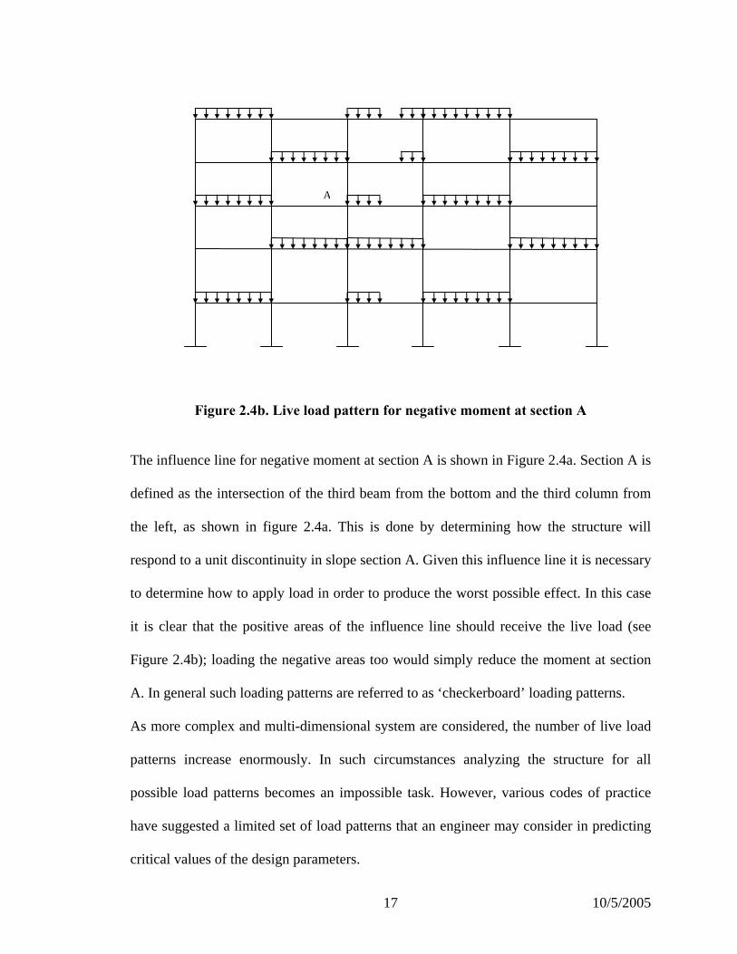
Figure 2.4b. Live load pattern for negative moment at section A
The influence line for negative moment at section A is shown in Figure 2.4a. Section A is
defined as the intersection of the third beam from the bottom and the third column from
the left, as shown in figure 2.4a. This is done by determining how the structure will
respond to a unit discontinuity in slope section A. Given this influence line it is necessary
to determine how to apply load in order to produce the worst possible effect. In this case
it is clear that the positive areas of the influence line should receive the live load (see
Figure 2.4b); loading the negative areas too would simply reduce the moment at section
A. In general such loading patterns are referred to as ‘checkerboard’ loading patterns.
As more complex and multi-dimensional system are considered, the number of live load
patterns increase enormously. In such circumstances analyzing the structure for all
possible load patterns becomes an impossible task. However, various codes of practice
have suggested a limited set of load patterns that an engineer may consider in predicting
critical values of the design parameters.
10/5/2005 17

From a practical point of view various codes of practices have suggested guidelines to
find the critical load patterns for typical members of the structure. The American
rally with the structure may be considered fixed.
In r
n all
actored loads on a single adjacent
columns and of
be considered fixed.
above and below the
Concrete Institute (ACI)’s code requirements for Structural Concrete and Commentary
while analyzing floor or roof member permits the load on a floor or roof member to be
Limited to combinations of factored dead load on all spans with full factored live
load on two adjacent spans.
Limited to combinations of factored dead load on all spans with full factored live
load on alternative spans.
Live load to be applied only to the floor or roof under consideration, and the far
ends of columns built integ
egard to the columns, ACI Code section 8.8 states:
Columns shall be designed to resist the axial forces from factored loads o
floors or roof and the maximum moment from f
span of the floor or roof under consideration. The loading condition giving the
maximum ratio of moment to axial load shall also be considered.
In frames or continuous construction, consideration shall be given to the effect of
unbalanced floor or roof loads on both exterior and interior
eccentric loading due to other causes.
In computing moments in columns due to gravity loading, the far ends of columns
built integrally with the structure may
The resistance to moments at any floor or roof level shall be provided by
distributing the moment between columns immediately
10/5/2005 18

given floor in proportion to the relative column stiffness and conditions of
restraint.
niform Building Code similarly states “the loading conditions which cause
um shear f
The U
maxim orce and bending moments along the member shall be investigated”.
It is important to note that for a 4 bay 40-story building, the total number of load patterns
that must be considered is 2160, which is about 1.5 ×1048. Such a calculation would be
ulation of interval
impossible even with the most extensive computational resources. Additionally, if an
engineer relies on analysis based on fewer conventional load patterns, he may not be able
to capture the critical scenario in the analysis and will be underestimating the response.
The safety of structure in such cases may be potentially compromised.
Interval finite element analysis, on the other hand, guarantees that the critical scenario
will be bounded in the sharp interval response. Before discussing form
finite element analysis, interval arithmetic needs to be reviewed. The next chapter focuses
on various developments in the area of interval arithmetic, basic features of interval
arithmetic and its application in engineering.
10/5/2005 19

3. INTERVAL ARITHMETIC
Early use of interval representation is associated with the treatment of truncation errors in
numerical calculations. For example, in a computational system with four decimal digits
accuracy, the number 4.1231 would be represented as an interval [4.123, 4.124]. This
approach allows the range of errors introduced by round-off errors to be precisely
determined. Moore (1966), instead of computing a numerical approximation using
limited-precision arithmetic, proceeded to construct intervals known in advance to
contain the desired results. Several authors have bound rounding errors using intervals
(Dwyer 1951; Sunaga 1958). However, Moore extended the use of interval analysis to
bind the effects of errors from different sources, including approximation errors and
errors in data.
Interval arithmetic was developed as an effective tool to obtain bounds on rounding and
approximation errors. It is still to be seen how effective this tool can be when the range of
the number is due to physical uncertainties instead of rounding errors.
A number of software libraries and extensions to programming language have been
developed to implement interval calculations using computers (Blecher et al. 1987;
Kullisch 1987). Additionally scientific calculators that are capable of dealing with
interval arithmetic operations in addition to normal arithmetic have been developed very
recently (GTREP at 2003).
Definitions of real intervals and operations with intervals can be found in a number of
references (Hansen 1965; Moor 1966; Alefeld and Herzberger 1983; Neumaier 1990).
10/5/2005 20

The fundamental concepts of interval arithmetic that has been seen in engineering
applications (Mullen and Muhanna 1999) are covered here.
An interval number is a closed set in R that includes the possible range of an unknown
real number, where R denotes the set of real numbers. A real interval is a set of the form
}~|~{:],[ ulul xxxRxxxx ≤≤∈=⇔
Based on the above definitions, interval arithmetic is defined on sets of intervals, rather
than on sets of real numbers. Interval mathematics can be considered a generalization of
real numbers mathematics. Overestimation is a major drawback in interval computations.
One reason is that only some of the algebraic laws, valid for real numbers, remain valid
for intervals; other laws hold only in a weaker form (Neumaier 1990, pp. 19-21). There
are two general rules for the algebraic properties of interval operations.
1. Two arithmetic expressions that are equivalent in real arithmetic, are equivalent in
interval arithmetic when a variable occurs only once on each side. In this case,
both sides yield the range of the expression. Consequently laws of commutativity,
associativity, and neutral elements are valid in Interval Arithmetic.
2. If f and g are two arithmetical expressions that are equivalent in real arithmetic,
then the inclusion holds, if every variable occurs only once in f. )()( xgxf ⊆
Also, a dependency problem arises when one or several variables occur more than once
in an interval expression. Dependency may lead to catastrophic overestimation in interval
computations. Precautions should be taken, if possible, to eliminate this effect.
Extending interval algebra in few more dimensions, it is easy to see that interval vectors
and interval matrices exist in this generalized space. An interval vector is a vector whose
components are interval numbers. An interval matrix is a matrix whose elements are
10/5/2005 21

interval numbers. The interval matrix contains all the real matrices, whose elements are
obtained from all possible values between the lower and upper bound of its interval
elements. One important type of the matrix in mechanics is symmetric matrices. A
symmetric interval matrix is one that contains only those real symmetric matrices whose
elements are obtained from all possible values between lower and upper bound of its
interval element. An interval vector is referred to as a box (Hansen 1992). The algebraic
properties of interval matrix operations are provided by Neumaier (1990), Apostolatos
and Kulisch (1968), and Mayer (1970).
Thus interval equations can be formed and solved for unknown interval variables. Such
formulations and solution algorithms become very efficient tools for analyzing a structure
if its relevant properties can be written as an interval. Subsequent chapters will introduce
a specific formulation that will be used for interval finite element analysis for load
combinations and load patterns. Since interval operations and equations require a
different kind of treatment, specific computer codes need to be developed in order to
solve large-scale problems.
In structural engineering interval arithmetic has already found various important
applications. Uncertainties in mechanics were introduced as interval values by Muhanna
and Mullen (2000). In such situations uncertain values were known to lie between two
values and formulations were developed in order to solve a system of equations that
involve interval quantities.
Although interval arithmetic was introduced by Moore (1966) and fuzzy sets theory by
Zadeh (1965), the application of interval concepts to structural analysis is more recent.
Koyluoglu, Cakmak and Nielson (1995) developed an interval approach utilizing the
10/5/2005 22

finite-element method to deal with pattern loading and structural uncertainties. The
solutions for the system of linear interval equations were obtained utilizing triangle
inequalities and linear programming. The results were conservative bounds for the
response quantities. Koyluoglu and Elishakoff (1998) introduced a comparison of
stochastic and interval finite elements applied to shear frame exhibiting uncertain
stiffness properties. Rao and Sawyer (1995), Rao and Berke (1997), and Rao and Chen
(1998) developed different versions of an interval based finite element method to account
for uncertainties in engineering problems. These publications were restricted to narrow
intervals and approximate numerical results.
A significant effort has been devoted in the work of Rao and Chen (1998) to develop a
new algorithm for the solution of linear interval equations. The developed algorithm used
search-based operations with an accelerated step size and an attempt to find an optimum
setting of unknown vector components.
Muhanna and Mullen (1995), Muhanna and Mullen (1996), Muhanna and Mullen (1999),
and Mullen and Muhanna (1999) developed a finite element analysis procedure that
utilizes the concept of fuzzy sets through interval calculations. They also computed the
response of different structural systems due to geometric and loading uncertainties.
Uncertainties were treated as possible values corresponding to a specific level of
presumption (α-cut). Results were exact in the case of load uncertainty and sharp for
geometric uncertainty. Exact bounds on possible node displacements and forces were
calculated by combinatorial calculations of all loading patterns, when computationally
feasible. This formulation has been the basis for the current thesis work. In the next
10/5/2005 23

section the above mentioned formulations of interval finite element analysis for interval
loads will be presented.
10/5/2005 24

4. INTERVAL FINITE ELEMENT ANALYSIS
Considering all the structural parameters as an interval number, a system of interval
equations can be formulated in general as
pqk =. (1)
Or in the following explicit form:
⎥⎥⎥⎥⎥⎥⎥⎥
⎦
⎤
⎢⎢⎢⎢⎢⎢⎢⎢
⎣
⎡
=
⎥⎥⎥⎥⎥⎥⎥⎥
⎦
⎤
⎢⎢⎢⎢⎢⎢⎢⎢
⎣
⎡
⎥⎥⎥⎥⎥⎥⎥⎥
⎦
⎤
⎢⎢⎢⎢⎢⎢⎢⎢
⎣
⎡
],[
],[
],[],[
],[
],[
],[],[
],[],[],[],[
],[],[],[],[
],[],[],[],[],[],[],[],[
ln
li
2l2
1l1
ln
li
2l2
1l1,
lnn
lnj2
ln21
ln1
lin
lij2
li21
li1
2l2n2
l2j22
l2221
l21
1l1n1
l1j12
l1211
l11
un
ui
u
u
un
ui
u
u
unn
unj
un
un
uin
uij
ui
ui
un
uj
uu
un
uj
uu
pp
pp
pppp
qqqq
kkkkkkkk
kkkkkkkk
kkkkkkkkkkkkkkkk
M
M
M
M
LL
MMMLMM
LL
MMMLMM
LL
LL
(2)
For the case of interval loads, the stiffness matrix k is the conventional deterministic
linear stiffness. The loading vector p will be interval quantity. The element generalized
forces and the generalized displacements will be linear transformations of the interval
quantities. In conventional finite-element formulations, the nodal load is given by
cb ppp += (3)
Where pc = vector of concentrated load; and pb = nodal load contribution from an element
and has the form
∑ ∫= dxxbNLp TTb )( (4)
Where L = Boolean connectivity matrix; b(x) =applied Traction; and Ni = shape function
for node i. Also note that pb itself can be broken in terms of element generalized nodal
loads pi .
10/5/2005 25

∫= dxxbNp Ti )( (5)
While analyzing a structure for load patterns and load combinations, only the function
b(x) (the magnitude of the load) is allowed to be an interval. To correctly evaluate
inclusive interval values for pi , attention must be paid to the sign of the terms Ni, as
whenever Ni is positive, upper limit of interval need to be integrated however whenever
Ni change sign to negative, the lower limit must be integrated.
As mentioned previously some of the conventional laws hold weakly in interval algebra,
care has to be given to the order of multiplication as otherwise it will have a strong
influence on the width of resulting intervals. One of the challenges that have to be faced
in interval algebra will be controlling the width of the interval. One way to control width
effectively will be delaying the use of interval values as much as possible.
It is important to see that some of the conventional characteristics of various analysis
parameters still have to be satisfied. As an example, shape function Ni(x) if selected as a
polynomial, automatically satisfies number of requirement of finite element for
convergence, compatibility, rigid body motion and stability. Additionally it is practical to
choose a loading function b(x) on element m in terms of an nth order polynomial:
∑=
=
=nj
j
jmj xAxb
0)( (6)
The element coefficient Amj for each term of the polynomial n on element m can be
written in matrix form as Fi with the dimension of (k × 1), where k is the number of
polynomial coefficients.
10/5/2005 26

⎟⎟⎟⎟⎟
⎠
⎞
⎜⎜⎜⎜⎜
⎝
⎛
=
An
AA
F i
i
iM
1
0
(7)
for i=1,2…m, where m = number of elements; for the whole system F can be expressed
as
⎟⎟⎟⎟⎟
⎠
⎞
⎜⎜⎜⎜⎜
⎝
⎛
=
mF
FF
FM2
1
(8)
Note that the dimension of F is [(m × k) × 1]
The pb vector now takes following form
MFpb = (9)
with the dimension of (ndof × 1), where ndof is number of degrees of freedom in the
system, and where
][ 21 mi MMMMM LL= (10)
with the dimension of [ndof × (m × k)]. The matrix Mi can be written as
[ ]niiiii QQQQM L210= (11)
Note that the dimension of Mi is (ndof × k). The expression for Qi may be given as
midxxNLQu
jTTi
ji L3,2,1=∀= ∫ (12)
And the dimension of Qi is (ndof × ndofel). ndofel is element’s number of degrees of
freedom.
These expressions have both real and interval numbers embedded in them. As such all
non-interval values are multiplied first and the last multiplication involves the interval
10/5/2005 27

quantities. In this process, width of resulting interval is reduced to the minimum possible
value.
Since the formulation of interval finite analysis is already in place, the next step will be to
see how uncertainty in the presence of live load can be handled using such formulation.
10/5/2005 28

5. LOAD TYPES AND INTERVAL TREATMENT
In the current conventional load pattern analysis and interval finite element analysis, the
following loads will be considered
1. Dead Load
2. Live Load
3. Earthquake Load
4. Wind Load
The dead loads and live loads are being considered as uniformly distributed load. Figure
3.1 shows that all the beams will be loaded all the time as far as dead load is considered.
Hence, in interval analysis the dead load will be taken as an interval load having lower
and upper bound equal to the magnitude of uniformly distributed dead load.
Figure 3.1. Dead Load Presence on a Portal Frame
10/5/2005 29

For load patterns involving live loads, the absence of load on a given member can be
Figure 3.2. Live load presence on a portal frame (checker-board pattern)
treated as a load of magnitude equal to zero and the presence of load can be treated as a
load of magnitude equal to its full value. Figure 3.2 indicates one of the live load patterns
that an engineer might choose for conventional structural analysis. Even under this
specific live load pattern, if required, uniformly distributed interval load can still be
assigned to all the beams. As an example, all the beams that are not loaded will have a
lower and upper bound of interval load equal to zero and the beams that are loaded will
have a lower and upper bound of interval to the magnitude of live load. This kind of
interval assignment will be needed for conventional load pattern analysis as the same
program is used for conventional and interval FE analysis, and thus it requires entire load
input to be interval quantities.
10/5/2005 30

Figure 3.3. Earthquake/Wind Load (Static Equivalent) presence on a portal frame
Figure 3.3 shows a typical earthquake and/or wind load acting on the frame structure.
oned above, structure need to be analyzed for number of load combinations.
+ L
L
These loads are always present on the structure. Hence, such loads will be treated as
deterministic loads in this work. In spite of their deterministic nature interval joint load
can still be assigned, with lower and upper bound equal to magnitude of joint load acting
on that joint. Such interval loads assignment will be needed as the program used to
perform conventional or interval finite element analysis requires loads to be input as an
interval.
As menti
However, if load factors in these load combinations are treated as interval quantities, such
load combinations can be combined into one interval equation. In current thesis work,
load combinations suggested by ASCE 2002 are being considered:
1.4 D
1.2 D
1.2 D + 1.6
10/5/2005 31

1.2 D + 0.8 W
1.2 D + 1.6 W + 1.0 L
It is ea t ad factor for dead load varies between 0.9 and 1.4, hence an
[0, 1.6]
ate load U can be written as
E
ter program that analyzes frame structures for conventional
1.2 D + 1.0 E + 1.0 L
0.9 D + 1.6 W
0.9 D + 1.0 E
sy o see that the lo
interval α with bounds between 0.9 and 1.4 can be assigned as interval load factor for
dead load. Similarly some of the load combinations don’t have any live load, however,
some of the load combinations have load factor for live load as high as 1.6. In this way an
interval load factor β i.e. [0, 1.6] can be assigned as an interval load factor for live load.
Continuing in the same direction, γ and δ can be defined an interval load factors for
earthquake load and wind load respectively.
α = [0.9, 1.4], β = [0, 1.6], γ = [0, 1] and δ =
Using these interval load factors, interval equation for ultim
U = α D + β L + γ EQ + δ W (13)
quation 13 contains all the load combination in itself. Later, interval finite element
analysis will be done for this interval equation and results in terms of the interval
response will be presented.
In the next chapter a compu
load pattern and interval FE analysis will be explored.
10/5/2005 32

6. C++ PROGRAM AND A TEST RUN
A C++ program has been developed in order to carry out conventional structural analysis
or interval finite element analysis for load patterns and load combinations. In this section,
various features of the program will be explored and later some test runs will be
presented in order to illustrate validity of the program.
This C++ program was initially written by Dr. Rafi Muhanna, Associate Professor at
Georgia Institute of Technology, Atlanta, for carrying out interval finite element analysis
under joint load and distributed load for frame element (See Appendix). The program was
designed to take care of one set of joint loads, dead load and live load. The program
accepts input load as deterministic and interval as well. The deterministic as well as the
interval response for each of the three loading cases are being produced separately as the
output file. To define response of the structure, bending moment, axial force and shear
force at start node and end nodes, maximum span moment and its location within span
and deflections of various joints are listed in the output file. This program was later been
re-structured by Hao Zhang, PhD student at Georgia Institute of Technology, to make it
efficient through the use of Object Oriented Programming.
The current analysis requires two types of joint loads (wind load and earthquake load)
and load combinations. As such, the program has been further enhanced to accommodate
two types of joint load and at the same time to accommodate load combinations involving
dead load, live load, earthquake load and wind load. In addition, load factors can be
entered as the interval quantities.
10/5/2005 33

In its current form, the program is capable of computing span moment, end moment,
shear force, axial force and deflection for various nodes or members for a given load
combination. The load factors are given as interval input, so whenever lower and upper
bound of the entire interval input is equal, the same program analyzes the structure for
deterministic loads.
As a part of object oriented programming, the program has a frame class and its objects
are created in main program. The frame class has been written in order to develop a
typical “frame” data structure and it encapsulates essential characteristic of a real frame
like number of nodes, number of members and various other parameters as protected
variables. Public methods have been provided in order to perform any necessary
operation like finding global stiffness matrix, incorporating boundary conditions,
calculating element forces and joint displacements. In the main part of program, an object
of frame is created and these public methods are called to perform interval finite element
analysis.
A number of test cases have been run and tested against manual results in order to verify
validity of this program, however only two such examples are being presented in this
section.
Example 1:
The first example focuses on load pattern analysis of a three spans continuous beam
under the application of live load (Figure 4.1a)
10/5/2005 34

1 2 3
4m 4m 4m
Live load = 6KN/m 4
Figure 4.1a. Finite Element consisting four nodes and three beam elements
The following structural parameters are given input data:
Cross-sectional area of the beam = 0.125 m2
Moment of inertia of the beam = 0.00260417 m4
Modulus of elasticity = 2 ×10⁶ KN/ m2
Live load = 6 KN/m
Length of each of the three spans = 4m
Here the envelope for bending moments due to live load pattern is being considered
throughout the beam. Maximum and minimum span moments and maximum and
minimum end moments are only needed in order to draw such envelope. Traditionally,
the engineer will be analyzing the structure under 23 (i.e. eight) live load patterns
(including no loading case). Taking combinations of presence and absence of live load on
every span, eight live load patterns can be generated. For this example, GTSTRUDL is
used in order to analyze the beam for all eight load patterns. Figure 4.1b shows the direct
output for the envelope of bending moments assembled from eight load patterns using
GTSTRUDL.
Interval finite element analysis is capable of determining this envelope in one run. As
stated in previous sections, absence and presence of live load on a span can be written as
zero value and full value of live load occurring on that span, respectively. If the live load
for every span is represented as an interval having bounds between zero and full value of
10/5/2005 35

live load at that span, the interval live load on the structure will contain all the
combinations of live load’s presence and absence; and hence the interval response will
capture all possible live load patterns in itself. So if an interval live load of [0, 6] KN/m is
assigned to each of the three spans, this beam once solved for interval load quantity using
finite element analysis, will give results accumulated from all the possible load patterns.
MZ ENVELOPE 9.72
-11.2
0.0
7.20
f-11.2
1.60 9.72
-11.2
1.60
0.0
X
Y
Meters KiloNewtons
Figure 4.1b. Moment envelope for all possible live load patterns (GTSTRUDL)
Table 1. Interval Finite Element Analysis results for three spans continuous beam
Interval span moment
Span 1 Span 2 Span 3
[-2.08, 9.707] [-4.8, 7.2] [-2.08, 9.707]
Interval end moment at start
Span 1 Span 2 Span 3
[0, 0] [-1.6, 11.2] [-1.6, 11.2]
Interval end moment at end
Span 1 Span 2 Span 3
Interval Finite
Element Analysis
[-11.2, 1.6] [-11.2, 1.6] [0, 0]
10/5/2005 36

It is important to note that interval maximum span moment bounds the results obtained
from the eight load patterns. Table 1 gives the result from finite element analysis under
the application of the interval load. It lists down interval response in terms of the interval
span moment, interval end moment at start and end section of the beam. The lower and
upper bounds of these interval end and span moments are in full agreement to the
moments shown in corresponding values of moment envelope obtained from
GTSTRUDL. However after the first decimal, slight difference between two results exists
because of the fineness of the mesh used in GTSTRUDL.
Example 2:
In this example the steel frame shown in Figure 5 is being analyzed first for interval load
application and later for various load combinations. The frame is under the application of
three concentrated loads. It is assumed that any of these three concentrated loads may be
present or absent at any time. This way these three joint loads lead to eight loading
scenarios. By introducing the three loads as intervals with values between zero and
maximum magnitude of the load, the entire eight-load scenario can be obtained in one
interval run. Interval finite analysis performed with the interval form of concentrated
loads captures all possible cases within the interval results. Here are the member
properties for the various finite elements.
Beam properties:
1. Section: W21×57
2. Cross-sectional Area = 16.7 in2 = 0.010774 m2
3. Moment of Inertia = 1170 in4 = 0.0004869 m4
Column properties:
10/5/2005 37

1. Section: W16×100
2. Cross-sectional Area = 29.7 in2 = 0.01916 m2
3. Moment of Inertia = 1500 in4 =0.0006243 m4
Due to the presence of concentrated load within the span, the frame is broken into five
finite elements.
Table 2 shows the results for axial force, shear force and moment at start and end nodes
of all the five finite element of this frame from interval FE analysis. Further, the same
frame has been analyzed for all the combination of presence and absence of each of the
three joint loads leading to eight conventional structural analyses. These results when
assembled to form an envelope give the maximum and minimum value of all the
structural parameters.
Table 3 shows the minimum and maximum value of these parameters. It is important to
note that table 2 and 3 are identical and it ensures the fact that interval finite element
analysis is capable of accounting for all load scenarios in the interval response of the
structure.
10/5/2005 38

15KN
20KN
8m
Element 4
5
Element 1
Element 2 Element 3 10KN
12m
Figure 5. Finite Ele
5m
ment cons
10m
isting five nodes and si
39
Element
x-frame element
10/5/2005

Table 2. Interval load input for interval finite element analysis
Interval Force Interval Moment
Node No. FX (KN) FY (KN) M z (KN-m)
1 [0, 0] [0, 0] [0, 0]
2 [0, 10] [0, 0] [0, 0]
3 [0, 0] [-15, 0] [0, 0]
4 [0, 0] [0, 0] [0, 0]
5 [-20, 0] [0, 0] [0, 0]
6 [0, 0] [0, 0] [0, 0]
10/5/2005 40

Table 3. Interval finite element analysis results for frame example (using C++ Program)
Element 1 2 3 4 5
FiX (KN) [-5.00487, 7.48309] [0, 12.4782] [0, 12.4782] [0, 12.4782] [-14.1157, 6.59393]
FiY (KN) [-5.08176, 12.0171] [-5.08176, 12.0171] [-12.5818, 4.51712] [-12.5818, 4.51712] [-12.5818, 4.51712]
MiZ (KN-m) [-48.7983, 34.6306] [-25.4278, 40.9988] [-24.7222, 5.61638] [-16.9692, 38.1866] [-40.5064, 11.8109]
FjX (KN) [-7.48309, 5.00487] [-12.4782, 0] [-12.4782, 0] [-12.4782, 0] [-6.59393, 14.1157]
FjY (KN) [-12.0171, 5.08176] [-12.0171, 5.08176] [-4.51712, 12.5818] [-4.51712, 12.5818] [-4.51712, 12.5818]
MjZ (KN-m) [-40.9988, 25.4278] [-5.61638, 24.7222] [-38.1866, 16.9692] [-11.8109, 40.5064] [-72.4193, 40.9405]
10/5/2005 41

Table 4. Conventional structural analysis results for frame example
Element 1 2 3 4 5
Conventional Analysis Min Max Min Max Min Max Min Max Min Max
FiX (KN) -5.00487 7.48309 0 12.4782 0 12.4782 0 12.4782 -14.1157 6.59393
FiY (KN) -5.08176 12.0171 -5.08176 12.0171 -12.5818 4.51712 -12.5818 4.51712 -12.5818 4.51712
MiZ (KN-m) -48.7983 34.6306 -25.4278 40.9988 -24.7222 5.61638 -16.9692 38.1866 -40.5064 11.8109
FjX (KN) -7.48309 5.00487 -12.4782 0 -12.4782 0 -12.4782 0 -6.59393 14.1157
FjY (KN) -12.0171 5.08176 -12.0171 5.08176 -4.51712 12.5818 -4.51712 12.5818 -4.51712 12.5818
MjZ (KN-m) -40.9988 25.4278 -5.61638 24.7222 -38.1866 16.9692 -11.8109 40.5064 -72.4193 40.9405
10/5/2005 42

7. INTERVAL ANALYSIS VS CONVENTIONAL ANALYSIS: LOAD COMBINATIONS & LOAD
PATTERNS
In this chapter a comparative study between conventional load pattern analysis and
interval finite element analysis will be performed through the analysis of a portal frame
for various load combinations and load patterns. A six-bay, seven-floor concrete frame
structure has been chosen. The frame will be analyzed first for selected load patterns with
specific load combinations; the response will be noted for selected members. Later, an
interval value will be assigned to live load and the frame will be analyzed for the same
load combinations, but this time under the application of interval load quantities using
interval finite element analysis.
Since conventional analysis involves analyzing a structure through specific load patterns,
various load patterns need to be considered. Ten load combinations are considered while
analyzing a column; however, beam is being limited to only three load combinations as
after study of several load combinations, not much deviation between two types of
analysis is reported. Hence columns in particular are the major emphasis of this section.
The analysis will cover several columns for axial force, shear force and maximum and
minimum end moment. The results for the beam are being shown only in terms of
maximum and minimum span moment. As there have been widely accepted load patterns
for getting maximum and minimum span moment, only those particulars patterns are
being considered for beams. For columns, three different load patterns have been chosen
for determining maximum positive and maximum negative end moment.
10/5/2005 43

7.1 Formulation
The formulation of the problem will begin with identification of various structural
parameters and important details of frame. In the next subsection, dead load, live load,
wind load and earthquake load will be computed; only critical calculations are shown
here.
27 inch
27 ft
27 ft
27 ft
27 ft
21 ft 21 ft 21 ft
27 ft
Figure 6.1. Typical floor plans
10/5/2005 44

The last subsections of current chapters provide the significant analysis results for various
finite elements. In the subsequent chapters these results will be assembled together in
order to perform a comparative analysis.
27 ft @each of 6 spans
11 ft 4 inch
Figure 6.2. Portal Frame in consideration (six bays & seven stories)
Figure 6.1 shows the plan of the building. Figure 6.2 gives the elevation of a s
seven-floor frame that is analyzed in subsequent subsection of this chapter.
numbering and member numbering is shown in Figure 6.3 and 6.4 respectively.
10/545
8ft 8 inch @eachof 5 spans
t
16 fix bay
Joint
/2005

Figure 6.3. Joints numbering for seven-floor frame
Figure 6.4. Frame elements numbering for seven-floor frame
7.1.1 Frame Data
Six bay Seven Floor Concrete Hospital Building -RCC
1
2
3
4
5
6
7
8 43
49
51 52 53 54 55
56
50
15 22 29 36
91 86
64
24
8 56
7 55
6 54
5 53
4 52
3 51
2 50
1 17 25 9 33 41 49
10/5/2005 46

Here are the various properties of the frame that may be of interest to the engineer. Since
the real data is being used, units for this frame will also follow the actual data, which is
an English standard.
1. Total Height = 70 ft 8 inch
2. Total span length = 162 ft
3. All beam are 24 inch by 1 8 inch
1. Cross-sectional Area A = 432 inch2
2. Moment of Inertia I xx = 20736 inch4
4. All columns are 30 inch by 30 inch
1. Cross-sectional Area A = 900 inch2
2. Moment of Inertia I xx = 67500 inch4
5. Modulus of elasticity for concrete is E concrete = 3600 ksi
7.1.2 Load Type/ Combinations:
The following load types and load combinations are being considered in current interval
finite element and conventional load pattern analysis.
1. Dead Load (D)
2. Live Load (L)
3. Earthquake Load (Static Equivalent) (EQ)
4. Wind load (W)
5. Load Combinations according to ASCE02
a. 1.4D
b. 1.2 D + 1.6 L
c. 1.2 D + L
10/5/2005 47

d. 1.2 D + 0.8 W
e. 1.2 D + 1.6 W + L
f. 1.2 D +/- 1.0 E + L
g. 0.9 D + /- 1.0 E
h. 0.9 D + 1.6 W
7.2 Load Computation
7.2.1 Dead Load and Live Load
Table 5 shows the location of building, seismic design category, type of frame, seismic
use group and computed dead load and live load.
Table 5. Dead load and live load for frame in consideration
Location: Atlanta, GA
Seismic Design Category: C
Seismic Use Group: III
Seismic Force Resisting System: Intermediate Reinforced Concrete Moment Frames
Thickness of Slab t = 10 inch
Density of concrete ρ = 0.15 k/ft3
Dead Load W DL = 18.2 k/ft
Live Load W LL = 18.0 k/ft
7.2.2 Earthquake Load
Table 6(a) shows important information that is needed in order to evaluate earthquake
load. Section 1615-1617 of IBC-16 is being used in order to evaluate earthquake load
present on frame.
10/5/2005 48

Table 6(b) shows contribution of every floor towards total statically equivalent joint
load present on frame.
Table 7 has the final statically equivalent joint load for earthquake load existing on
the five-story structure.
Table 6a. Computation of earthquake load
Weight of the Structure W = 4000 Kips
Design Spectral Response Acceleration at Short Period SDS = 0.1387 g
Response Modification Factor R = 4.5
Importance Factor IE = 1.5
Number of floors N = 7
Natural Time Periods T =0.1N = 0.7 seconds
If T < 0.5 sec => k = 1 & If T > 2.5 sec => k = 2
Interpolating for values of k in between for T = 0.7 => k = 1.1
As per the “Equivalent Lateral Force Procedure” of the International Building Code,
the static equivalent of the total earthquake load acting at structure is being given as
WCV s ×= (14)
Where Cs is being given as:
E
DSs IR
SC
/= (15)
And W is the weight of the structure.
For the structure being considered, Cs turns out to be 0.0831.
Vertical distribution of equivalent static earthquake force is given as
10/5/2005 49

VCF VXx ×= (16)
where V is the total design lateral force or shear. Note that the parameter CVX accounts
for the vertical distribution of equivalent static forces. The “Equivalent Lateral Force
Procedure” gives the following expression in order to evaluate CVX.
∑=
×
×= N
i
kii
kix
VX
hw
hwC
1
(17)
where hi is the height from base to level i and N is the number of stories in frame.
Considering the symmetric nature of frame with respect to all floors, weight of the
frame W is distributed equally among all floors.
If wi is the weight corresponding to ith floor and n are the total number of floors then
ninWwi ...1/ =∀=⇒ (18)
Table 6b. Computation of earthquake load (cont.)
Story Story Height Story Height from Base hi hi k CVX
1 16 16 21.11 0.04
2 8.66 24.66 33.98 0.07
3 8.66 33.33 47.33 0.10
4 8.66 42 61.03 0.14
5 8.66 50.66 75.02 0.17
6 8.66 59.33 89.25 0.20
7 11.33 70.66 108.17 0.24
Summation 435.92
10/5/2005 50

Table 7. Earthquake loads as statically equivalent joint load
Static Equivalent of Earthquake Load: QE
W = 4000 Kips
Cs = 0.0831
V = 332.4 Kips
Floor i Joint Load At floor i, Vi (kips)
1 16.09
2 25.91
3 36.09
4 46.54
5 57.20
6 68.05
7 82.48
7.2.3 Wind Load
Section 6 of ASCE-7/2002 is used to develop appropriate static equivalent joint loads for
wind load acting on the frame in consideration.
The minimum wind load = 10 lb/ft2 is multiplied by the area of the building or structure
projected on a vertical plane normal to the wind direction.
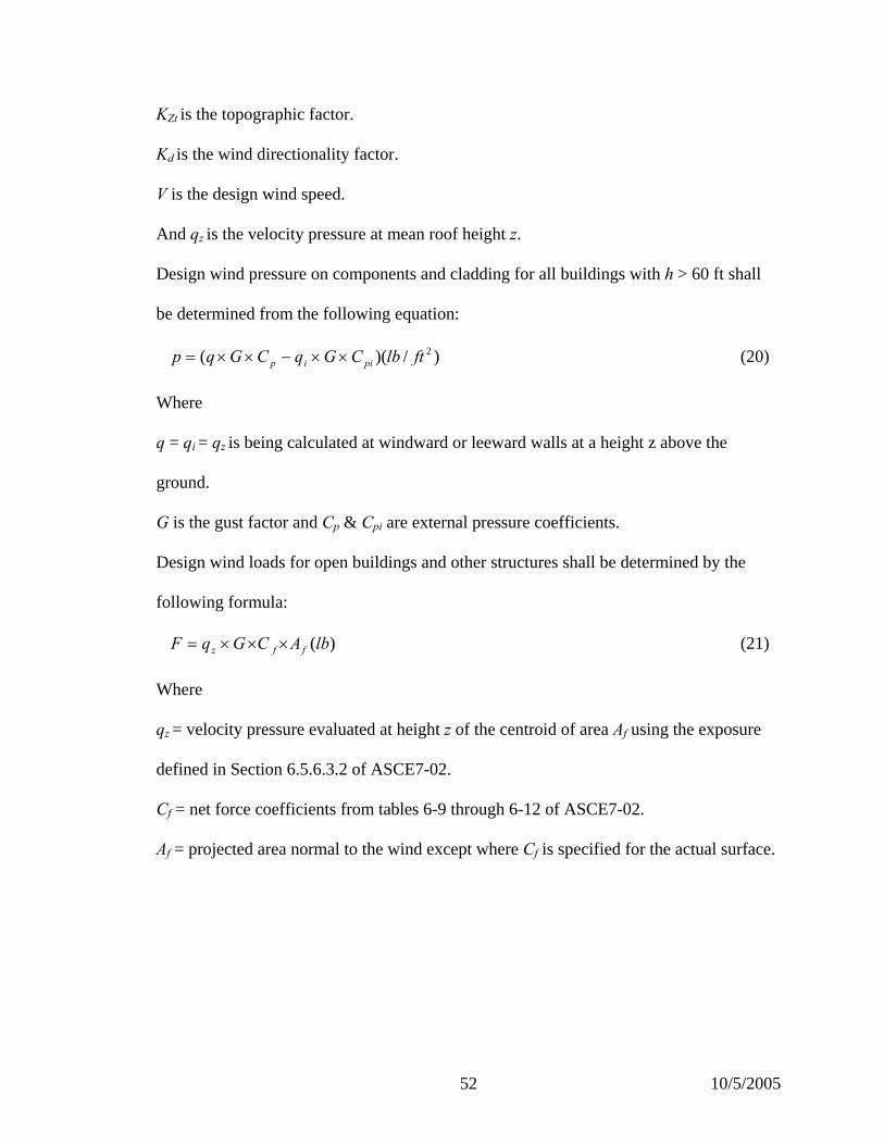
As per the Section 6.5.10 of ASCE-7/2002, velocity pressure, qZ evaluated at height z
shall be calculated by the following equation:
)/(00256.0 22 ftlbIVKKKq dZtZz ×××××= (19)
where
KZ is the velocity pressure exposure coefficient.
10/5/2005 51
KZt is the topographic factor.
Kd is the wind directionality factor.
V is the design wind speed.
And qz is the velocity pressure at mean roof height z.
Design wind pressure on components and cladding for all buildings with h > 60 ft shall
be determined from the following equation:
)/)(( 2ftlbCGqCGqp piip ××−××= (20)
Where
q = qi = qz is being calculated at windward or leeward walls at a height z above the
ground.
G is the gust factor and Cp & Cpi are external pressure coefficients.
Design wind loads for open buildings and other structures shall be determined by the
following formula:
)(lbACGqF ffz ×××= (21)
Where
qz = velocity pressure evaluated at height z of the centroid of area Af using the exposure
defined in Section 6.5.6.3.2 of ASCE7-02.
Cf = net force coefficients from tables 6-9 through 6-12 of ASCE7-02.
Af = projected area normal to the wind except where Cf is specified for the actual surface.
10/5/2005 52

Table 8a. Wind pressure calculations
Wind Pressure Calculations Method 2: Analytical procedure from ASCE 7-98
Basic Wind Speed, V (mph) = 90 Exposure: A
Importance Factor, I = 1.15 Wind Directionality Factor, Kd = 0.85
Kzt = 1 Gf = 0.85
For Exposure A, α= 5 Zg (ft.) = 1500
Table 8b. Wind pressure calculations (cont.)
Calculate Kz & qz for each height
Floor Level Height (ft) Z (ft.) Kz qz (lbs/ft2) Foundation 0 0 0.680 16.22
1 16 16 0.680 16.22 2 8.66 24.66 0.680 16.22 3 8.66 33.33 0.680 16.22 4 8.66 42 0.680 16.22 5 8.66 50.67 0.680 16.22 6 8.66 59.33 0.680 16.22
Roof 11.33 70.67 0.680 16.22 L/B Cp L/B Cp 2 -0.3
L (ft) 162 2.57 X B (ft) 63 4 -0.2 Cp -0.27
Tables 8 (a), 8 (b) and 8 (c) give the calculations done in order to obtain the statically
equivalent joint loads for wind loads present on a seven-story frame. Table 9 contains the
final wind load present on the frame in consideration.
10/5/2005 53

Table 8c. Wind pressure calculations (cont.)
Calculate the wind pressure from the two directions Wind From Ends pz (psf)
Z (ft.) Windward End Leeward End Sides Total pz (psf) L/B = 2.57 Cp = 0.8 Cp = -0.271 Cp = -0.7
0 11.03 -3.74 -9.65 14.77 16 11.03 -3.74 -9.65 14.77
24.66667 11.03 -3.74 -9.65 14.77 33.33333 11.03 -3.74 -9.65 14.77
42 11.03 -3.74 -9.65 14.77 50.67 11.03 -3.74 -9.65 14.77 59.33 11.03 -3.74 -9.65 14.77 70.67 11.03 -3.74 -9.65 14.77
Table 9. Static equivalent of wind load
Calculate the static equivalent of wind pressure Effective Width 21
Height Pressure Design Wind Load Ft Psf Kips 0 14.77
16 14.77 4.96 24.66 14.77 2.68 33.33 14.77 2.68
42 14.77 2.68 50.67 14.77 2.68 59.33 14.77 2.68 70.67 14.77 3.51
Table 10 summarizes earthquake load and wind load as statically equivalent joint load
occurring on various joints.
10/5/2005 54
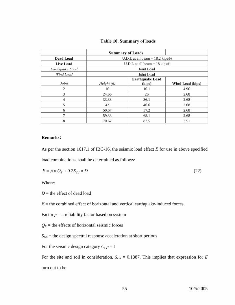
Table 10. Summary of loads
Summary of Loads Dead Load U.D.L at all beam = 18.2 kips/Ft Live Load U.D.L at all beam = 18 kips/ft
Earthquake Load Joint Load Wind Load Joint Load
Joint Height (ft) Earthquake Load
(kips) Wind Load (kips) 2 16 16.1 4.96 3 24.66 26 2.68 4 33.33 36.1 2.68 5 42 46.6 2.68 6 50.67 57.2 2.68 7 59.33 68.1 2.68 8 70.67 82.5 3.51
Remarks:
As per the section 1617.1 of IBC-16, the seismic load effect E for use in above specified
load combinations, shall be determined as follows:
DSQE DSE ×+×= 2.0ρ (22)
Where:
D = the effect of dead load
E = the combined effect of horizontal and vertical earthquake-induced forces
Factor ρ = a reliability factor based on system
QE = the effects of horizontal seismic forces
SDS = the design spectral response acceleration at short periods
For the seismic design category C, ρ = 1
For the site and soil in consideration, SDS = 0.1387. This implies that expression for E
turn out to be
10/5/2005 55

DQE E ×+= 02774.0 (23)
Note that, E once included in the expressions of load combination, will modify the load
factors of Dead Load and Horizontal Seismic Loads as computed above.
Sign Convention:
Figure 7.0. Sign convention for positive and negative bending moment
10/5/2005 56

7.3 Comparative Analysis for Load Patterns & Load Combinations
7.3.1 Case 1-Maximum Span Moment in a beam
In this case the maximum span moment in beam 64 (figure 7.1) is the current design
parameter. Using the general principle of influence the structure may be analyzed for this
particular live load pattern in association with a number of load combinations:
64
Figure 7.1. Case 1: Live load pattern for maximum span moments in beam
Table 11. Maximum Span Moment in beam
Beam 64 Interval Analysis Conventional Analysis
Load Combination Interval Span Moment (kips-inch) Maximum Span Moment (kips-inch)
1.4D [9295, 9295] 9295
1.2D+1.6L [7016,19420] 19410
1.2D+L [7373,15130] 15120
10/5/2005 57

Maximum span moments obtained from conventional load patterns are within the interval
span moment calculated using interval FE analysis (Table 11). This shows enclosure of
conventional result in the interval FE analysis result. It is important to note that not only
this particular load pattern is bounded by the enclosure, but every load as well. Span
moment is chosen as one of the representative parameters in this case. One more
parameter, end moment, will also be considered in a subsequent section. However,
deflection at any point, shear force and axial force are all equally valid parameters that
can be chosen to demonstrate this kind of concept.
7.3.2 Case 2-Minimum Span Moment in a beam
In this case the minimum moment at the starting node of beam 64 (figure 7.2) is the
current design parameter. Using the general principle of influence lines structure may be
analyzed for this particular live load pattern in association with a number of load
combinations:
64
Figure 7.2. Case 2: Live load pattern for minimum span moment in beam
10/5/2005 58

Table 12. Minimum Span Moment in beam
Beam 64 Interval Analysis Conventional Analysis
Load Combination Interval Span Moment (kips-inch) Minimum Span Moment (kips-inch)
1.4D [9295, 9295] 9295
1.2D+1.6L [7016,19420] 7028
1.2D+L [7373,15130] 7380
Once again, enclosure of the results from the load pattern chosen for minimum span
moment in a beam, within the results from Interval FE Analysis, can be seen. The results
in table 12 indicate that the minimum span moment obtained from live load pattern is
within the interval value of span moment computed using interval finite element analysis.
In these cases only three load combinations have been considered, but in the next section
column is analyzed for 10 load combinations to show the general tendency of getting
enclosure within interval FE results.
7.3.3 Case 3- Maximum/Minimum End Moments in a Column
In this case maximum end moment of a column is the current design parameter. End
moments for column 1, 4, 7 and 8 will be presented. Using general principle of influence
lines structure may be analyzed for some definite live load pattern in association with
number of load combinations. Here are three widely used load patterns that will be
considered for maximum and minimum end moment in the column:
10/5/2005 59

Figure 7.3. Case 3: Live load pattern A for maximum/minimum end moment in a column
Figure 7.4. Case 3: Live load pattern B for maximum/minimum end moment in a column
8 1
4
7
8
7
4
1
10/5/2005 60

8
7
4
1
Figure 7.5. Case 3: Live load pattern C for maximum/minimum end moment in a column
10/5/2005 61

Table 13 End Moment in column element 8 as an effect of Live Load pattern A, B and C
Column 8 Interval Analysis Conventional Analysis Conventional Analysis Conventional Analysis
Load Combination Interval End
Moment (kips-inch)
End Moments
(kips-inch)
Load Pattern “A”
End Moments
(kips-inch)
Load Pattern “B”
End Moments
(kips-inch)
Load Pattern “C”
1.4D [-1293, -1293] -1293 -1293 -1293
1.2D+1.6L [-12193.5, 8515.77] 4927.87 -8307.41 -11568.9
1.2D+L [-8036.55, 4906.75] 2664.31 -5607.74 -7646.14
1.2D+0.8W [-955.202, -955.202] -955.202 -955.202 -955.202
1.2 D + 1.6 W + L [-7730.38, 5212.92] 2970.49 -5301.56 -7339.97
1.2 D + 1.0 E1 + L [-5591.51, 7351.79] 5109.36 -3162.69 -5201.09
1.2 D + 1.0 E2 + L [-5563.06, 7380.24] 5137.8 -3134.25 -5172.65
0.9 D + 1.0 E1 [1590.55, 1590.55] 1590.55 1590.55 1590.55
0.9 D + 1.0 E2 [1642.27, 1642.27] 1642.27 1642.27 1642.27
0.9 D + 1.6 W [-525.043, -525.043] -525.043 -525.043
load factors as Interval [-15419.8, 14588.3]
Figure 7.3, 7.4 and 7.5 shows the live load pattern A, B and C respectively, used in order
to calculate end moment in various columns. Table 13 focuses on column element 8 and
gives the interval end moment obtained from Interval Finite Element Analysis and end
moments from load pattern A, B and C respectively. The last row of the table 13 shows
the interval end moment at the end of column 8 as per the interval load factors. In this
particular case, all the load combinations have been combined into one interval equation
and interval finite element analysis is done under one interval load combination equation.
10/5/2005 62

The interval end moments obtained in this way contain all the interval end moments that
are obtained from specific load combination.
Table 14. Axial Force in column 8 as an effect of Live Load pattern A, B and C
Column 8 Interval Analysis Conventional Analysis Conventional Analysis Conventional Analysis
Load Combination Interval Axial force
(kips)
Axial Force (kips)
Load Pattern “A”
Axial Force (kips)
Load Pattern “B”
Axial Force (kips)
Load Pattern “C”
1.4D [4798.24, 4798.24] 4798.24 4798.24 4798.24
1.2D+1.6L [4110.8, 9537] 6837.8 6821.76 6826.16
1.2D+L [4111.54, 7502.92] 5815.91 5805.89 5808.64
1.2D+0.8W [4112.82, 4112.82] 4112.82 4112.82 4112.82
1.2 D + 1.6 W + L [4111.64, 7503.01] 5816.01 5805.98 5808.74
1.2 D + 1.0 E1 + L [4123.01, 7514.38] 5827.38 5817.36 5820.11
1.2 D + 1.0 E2 + L [4017.45, 7408.82] 5721.82 5711.8 5714.55
0.9 D + 1.0 E1 [3182.42, 3182.42] 3182.42 3182.42 3182.42
0.9 D + 1.0 E2 [2990.49, 2990.49] 2990.49 2990.49 2990.49
0.9 D + 1.6 W [3084.68, 3084.68] 3084.68 3084.68 3084.68
Load factors as Interval [3081.83, 10225.2]
The interval axial forces obtained from interval finite element analysis and axial force
from load pattern A, B and C respectively for column element 8 are given in table 14. It
is important to note that as shown for interval span moment, the interval response for
axial force again bounds conventional results. The last row of Table 14 and Table 15
show the interval axial force and interval shear force when load factors are taken as
interval. Interval shear force obtained from interval load factor equation, bounds all the
10/5/2005 63

interval shear force that is obtained using finite element analysis for a given load
combination. Note that load pattern A results in the maximum axial force in column 8 for
all the load combinations; this is the same load pattern that resulted in the maximum
positive end moment in the same column (Table 13 and 14). Table 13 shows that the
maximum negative moment for the column in consideration occurs due to load pattern C.
However, this load pattern does not yield the maximum axial force. The three load
patterns used here are the most popular ones, do not necessarily give the critical scenario;
however, interval results will always capture critical response of the structure.
Table 15. Shear Force in column 8 as an effect of Live Load pattern A, B and C
Column 8 Interval Analysis Conventional Analysis Conventional Analysis Conventional Analysis
Load Combination Interval Shear force
(kips)
Shear Force (kips)
Load Pattern A
Shear Force (kips)
Load Pattern B
Shear Force (kips)
Load Pattern C
1.4D [13.2359, 13.2359] 13.2359 13.2359 13.2359
1.2D+1.6L [-63.0328, 100.68] -35.014 71.1735 94.8429
1.2D+L [-35.1411, 67.1795] -17.6294 48.7378 63.5312
1.2D+0.8W [8.59973, 8.59973] 8.59973 8.59973 8.59973
1.2 D + 1.6 W + L [-40.6318, 61.6888] -23.12 43.2472 58.0406
1.2 D + 1.0 E1 + L [-85.0459, 17.2747] -67.5342 -1.16695 13.6264
1.2 D + 1.0 E2 + L [-85.3371, 16.9835] -67.8254 -1.45814 13.3353
0.9 D + 1.0 E1 [-41.1578, -41.1578] -41.1578 -41.1578 -41.1578
0.9 D + 1.0 E2 [-41.6872, -41.6872] -41.6872 -41.6872 -41.6872
0.9 D + 1.6 W [3.01813, 3.01813] 3.01813 3.01813 3.01813
Load factors as Interval [-144.797, 126.077]
10/5/2005 64

Table 15 indicates how different shear force values obtained from load pattern A, B and
C are contained within the interval shear force calculated using interval finite element
analysis. Table 13, Table 14 and Table 15 clearly show that the end moments, axial force
and shear force in column 8 obtained from specific live load patterns are non-
conservative.
Additionally similar results are presented for few selected columns present at 1st, 4thand
7th floor. Columns 1, 4 and 7 have been chosen from these floors. For each of the load
combinations, table 16 gives interval end moments and end moments in column 1
obtained from three live load pattern. Table 17 and Table 18 provide the similar results
for axial force and shear force in column 1. Table 19, 20 and 21 present a comparison of
interval response in terms of the end moment, axial force and shear force in column 4
with corresponding conventional load pattern analysis results. Similar results are
presented for column 7 in Table 22, Table 23 and Table 24.
10/5/2005 65

Table 16. End Moment in column 1 as an effect of Live Load A, B and C
Column 1 Interval Analysis Conventional
Analysis
Conventional
Analysis
Conventional Analysis
Load Combination Interval End
Moment (kips-inch)
End Moments
(Kips-inch)
Load Pattern A
End Moments
(Kips-inch)
Load Pattern B
End Moments
(Kips-inch)
Load Pattern C
1.4D [-8097.51, -8097.51] -8097.51 -8097.51 -8097.51
1.2D+1.6L [-17727.6, -5304.45] -15045.4 -7840.98 -6373.14
1.2D+L [-13682.5, -5918.05] -12006.1 -7503.38 -6332.37
1.2D+0.8W [-6813.91, -6813.91] -6813.91 -6813.91 -6813.91
1.2 D + 1.6 W + L [-13428.9, -5664.43] -11752.5 -7249.77 -6332.37
1.2 D + 1.0 E1 + L [-12164.6, -4400.18] -10488.2 -5985.51 -5068.11
1.2 D + 1.0 E2 + L [-11986.5, -4222.03] -10310.1 -5807.36 -4889.96
0.9 D + 1.0 E1 [-3833.42, -3833.42] -3833.42 -3833.42 -3833.42
0.9 D + 1.0 E2 [-3509.52, -3509.52] -3509.52 -3509.52 -3509.52
0.9 D + 1.6 W [-4951.92, -4951.92] -4951.92 -4951.92 -4951.92
Load factors as Interval [-19401.5, -1264.45]
10/5/2005 66

Table 17. Axial Force in column 1 as an effect of Live Load pattern A, B and C
Column 1 Interval Analysis Conventional
Analysis
Conventional
Analysis
Conventional
Analysis
Load Combination Interval Axial
force (kips)
Axial Force (kips)
Load Pattern A
Axial Force (kips)
Load Pattern B
Axial Force (kips)
Load Pattern C
1.4D [2420.95, 2420.95] 2420.95 2420.95 2420.95
1.2D+1.6L [2063.23, 4822.78] 4794.58 3249.73 3246.95
1.2D+L [2067.68, 3792.4] 3774.77 2809.24 2801.13
1.2D+0.8W [2071.92, 2071.92] 2071.92 2071.92 2071.92
1.2 D + 1.6 W + L [2061.31, 3786.02] 3768.4 2802.87 2801.13
1.2 D + 1.0 E1 + L [1991.28, 3716] 3698.37 2732.84 2731.11
1.2 D + 1.0 E2 + L [1938.02, 3662.74] 3645.11 2679.58 2677.85
0.9 D + 1.0 E1 [1523.51, 1523.51] 1523.51 1523.51 1523.51
0.9 D + 1.0 E2 [1426.67, 1426.67] 1426.67 1426.67 1426.67
0.9 D + 1.6 W [1549.95, 1549.95] 1549.95 1549.95 1549.95
Load factors as Interval [1453.08, 5172.38]
10/5/2005 67

Table 18. Shear Force in column 1 as an effect of Live Load pattern A, B and C
Column 1 Interval Analysis Conventional Analysis Conventional Analysis Conventional Analysis
Load Combination Interval Shear
force (kips)
Shear Force (kips)
Load Pattern A
Shear Force (kips)
Load Pattern B
Shear Force (kips)
Load Pattern C
1.4D [68.7488, 68.7488] 68.7488 68.7488 68.7488
1.2D+1.6L [48.8848, 146.66] 126.165 68.7097 58.4322
1.2D+L [52.6509, 113.76] 100.951 65.0414 53.4437
1.2D+0.8W [56.3404, 56.3404] 56.3404 56.3404 56.3404
1.2 D + 1.6 W + L [47.4766, 108.586] 95.7765 59.8672 53.4437
1.2 D + 1.0 E1 + L [9.97928, 71.0887] 58.2792 22.3698 15.9464
1.2 D + 1.0 E2 + L [8.4668, 69.5762] 56.7667 20.8574 14.4339
0.9 D + 1.0 E1 [2.76157, 2.76157] 2.76157 2.76157 2.76157
0.9 D + 1.0 E2 [0.0116125,
0.0116125]
0.0116125 0.0116125 0.0116125
0.9 D + 1.6 W [39.0214, 39.0214] 39.0214 39.0214 39.0214
Load factors as Interval [-17.0043, 159.655]
10/5/2005 68

Table 19. End Moment in column element 4 as an effect of Live Load pattern A, B and C
Column 4 Interval Analysis Conventional
Analysis
Conventional
Analysis
Conventional
Analysis
Load Combination Interval End
Moment (kips-inch)
End Moments
(Kips-inch)
Load Pattern A
End Moments
(Kips-inch)
Load Pattern B
End Moments
(Kips-inch)
Load Pattern C
1.4D [-9584.83, -9584.83] -9584.83 -9584.83 -9584.83
1.2D+1.6L [-21985.5, -5276.96] -18564.9 -20517.3 -18843.5
1.2D+L [-16821.8, -6378.94] -14683.9 -15904.2 -14717.2
1.2D+0.8W [-8145.17, -8145.17] -8145.17 -8145.17 -8145.17
1.2 D + 1.6 W + L [-16681, -6238.15] -14543.1 -15763.4 -14717.2
1.2 D + 1.0 E1 + L [-15110.6, -4667.73] -12972.7 -14192.9 -13146.8
1.2 D + 1.0 E2 + L [-14899.7, -4456.86] -12761.8 -13982.1 -12936
0.9 D + 1.0 E1 [-4623, -4623] -4623 -4623 -4623
0.9 D + 1.0 E2 [-4239.6, -4239.6] -4239.6 -4239.6 -4239.6
0.9 D + 1.6 W [-6020.89, -6020.89] -6020.89 -6020.89 -6020.89
Load factors as Interval [-24319, -387.651]
10/5/2005 69

Table 20. Axial Force in column element 4 as an effect of Live Load pattern A, B and C
Column 4 Interval Analysis Conventional Analysis Conventional Analysis Conventional Analysis
Load Combination Interval Axial force
(kips)
Axial Force (kips)
Load Pattern A
Axial Force (kips)
Load Pattern B
Axial Force (kips)
Load Pattern C
1.4D [1385.81, 1385.81] 1385.81 1385.81 1385.81
1.2D+1.6L [1175.96, 2765.75] 2741.33 1973.25 1971.89
1.2D+L [1180.42, 2174.03] 2158.77 1678.72 1675.45
1.2D+0.8W [1186.63, 1186.63] 1186.63 1186.63 1186.63
1.2 D + 1.6 W + L [1177.99, 2171.61] 2156.35 1676.3 1675.45
1.2 D + 1.0 E1 + L [1148.5, 2142.12] 2126.86 1646.81 1645.96
1.2 D + 1.0 E2 + L [1118.02, 2111.63] 2096.37 1616.32 1615.47
0.9 D + 1.0 E1 [883.911, 883.911] 883.911 883.911 883.911
0.9 D + 1.0 E2 [828.479, 828.479] 828.479 828.479 828.479
0.9 D + 1.6 W [888.457, 888.457] 888.457 888.457 888.457
Load factors as Interval [838.144, 2967.48]
10/5/2005 70

Table 21. Shear Force in column 4 as an effect of Live Load pattern A, B and C
Column 4 Interval Analysis Conventional Analysis Conventional Analysis Conventional Analysis
Load Combination Interval Shear force
(kips)
Shear Force (kips)
Load Pattern A
Shear Force (kips)
Load Pattern B
Shear Force (kips)
Load Pattern C
1.4D [186.075, 186.075] 186.075 186.075 186.075
1.2D+1.6L [111.718, 417.541] 360.488 396.684 264.905
1.2D+L [129.634, 320.773] 285.115 307.737 223.791
1.2D+0.8W [158.7, 158.7] 158.7 158.7 158.7
1.2 D + 1.6 W + L [128.049, 319.188] 283.53 306.152 223.791
1.2 D + 1.0 E1 + L [107.52, 298.66] 263.001 285.624 203.262
1.2 D + 1.0 E2 + L [103.427, 294.566] 258.908 281.53 199.169
0.9 D + 1.0 E1 [100.856, 100.856] 100.856 100.856 100.856
0.9 D + 1.0 E2 [93.4126, 93.4126] 93.4126 93.4126 93.4126
0.9 D + 1.6 W [118.035, 118.035] 118.035 118.035 118.035
Load factors as Interval [26.1216, 465.777]
10/5/2005 71

Table 22. End Moment in column 7 as an effect of Live Load pattern A, B and C
Column 7 Interval Analysis Conventional
Analysis
Conventional
Analysis
Conventional
Analysis
Load Combination Interval End
Moment (kips-
inch)
End Moments
(Kips-inch)
Load Pattern A
End Moments
(Kips-inch)
Load Pattern B
End Moments
(Kips-inch)
Load Pattern C
1.4D [-17120, -17120] -17120 -17120 -17120
1.2D+1.6L [-35710.4, -12984.6] -33965.2 -34342.1 -16521.6
1.2D+L [-27821.8, -13618.2] -26731.1 -26966.7 -14459
1.2D+0.8W [-14645.1, -14645.1] -14645.1 -14645.1 -14645.1
1.2 D + 1.6 W + L [-27763.5, -13559.9] -26672.7 -26908.3 -14459
1.2 D + 1.0 E1 + L [-27012.3, -12808.7] -25921.6 -26157.1 -13707.8
1.2 D + 1.0 E2 + L [-26635.7, -12432.1] -25544.9 -25780.5 -13331.2
0.9 D + 1.0 E1 [-10504.3, -10504.3] -10504.3 -10504.3 -10504.3
0.9 D + 1.0 E2 [-9819.55, -9819.55] -9819.55 -9819.55 -9819.55
0.9 D + 1.6 W [-10947.4, -10947.4] -10947.4 -10947.4 -10947.4
Load factors as Interval [-38690.1, -7879.94]
10/5/2005 72

Table 23. Axial Force in column 7 as an effect of Live Load pattern A, B and C
Column 7 Interval Analysis Conventional
Analysis
Conventional
Analysis
Conventional
Analysis
Load Combination Interval Axial
force (kips)
Axial Force (kips)
Load Pattern A
Axial Force (kips)
Load Pattern B
Axial Force (kips)
Load Pattern C
1.4D [338.857, 338.857] 338.857 338.857 338.857
1.2D+1.6L [275.775, 688.048] 676.414 681.523 282.461
1.2D+L [281.278, 538.948] 531.677 534.87 285.108
1.2D+0.8W [290.274, 290.274] 290.274 290.274 290.274
1.2 D + 1.6 W + L [280.929, 538.599] 531.328 534.521 285.108
1.2 D + 1.0 E1 + L [276.904, 534.574] 527.303 530.496 281.082
1.2 D + 1.0 E2 + L [269.449, 527.119] 519.848 523.041 273.627
0.9 D + 1.0 E1 [219.562, 219.562] 219.562 219.562 219.562
0.9 D + 1.0 E2 [206.007, 206.007] 206.007 206.007 206.007
0.9 D + 1.6 W [217.488, 217.488] 217.488 217.488 217.488
Load factors as Interval [193.125, 741.093]
10/5/2005 73

Table 24. Shear Force in column 7 as an effect of Live Load pattern A, B and C
Column 7 Interval Analysis Conventional Analysis Conventional Analysis Conventional Analysis
Load Combination Interval Shear
force (kips)
Shear Force (kips)
Load Pattern A
Shear Force (kips)
Load Pattern B
Shear Force (kips)
Load Pattern C
1.4D [193.168, 193.168] 193.168 193.168 193.168
1.2D+1.6L [129.096, 420.338] 385.646 333.921 227.535
1.2D+L [142.775, 324.801] 303.119 270.79 203.878
1.2D+0.8W [165.362, 165.362] 165.362 165.362 165.362
1.2 D + 1.6 W + L [142.353, 324.379] 302.697 270.369 203.878
1.2 D + 1.0 E1 + L [137.617, 319.642] 297.96 265.632 194.891
1.2 D + 1.0 E2 + L [133.367, 315.393] 293.711 261.382 194.891
0.9 D + 1.0 E1 [122.498, 122.498] 122.498 122.498 122.498
0.9 D + 1.0 E2 [114.771, 114.771] 114.771 114.771 114.771
0.9 D + 1.6 W [123.758, 123.758] 123.758 123.758 123.758
Load factors as Interval [62.6055, 467.065]
10/5/2005 74

Table 16, 19 and 22 show that for a given load combination and a given load pattern, end
moments increase from lower floor columns to upper floor columns. However table 17,
20 and 23 shows that axial force decreases from lower level columns to upper level
columns. Additionally, the same nature of behavior can be observed for the lower and
upper bounds of the interval response. Alternatively, it can be deduced that for a given
load combination and a given load pattern, the lower bound on end moments decreases
from lower level columns to upper level columns and at the same time the upper bound
on column end moments increase from lower level column to upper level column.
Consequently, for a given load combination that involves a live load, the width of the
interval moments increases from lower level column to upper level column.
10/5/2005 75

8. COMPARATIVE STUDY OF INTERVAL FE & CONVENTIONAL ANALYSIS: EFFECTS OF
NUMBER OF FLOOR
In this section, structure will be analyzed for varying height and objective is to identify
the nature of deviation between interval response and conventional structural response.
The frame that we have been using since last section will be considered once again. This
frame will be modified to increase number of floors up to ten and fifteen. Structure will
be analyzed under various load combinations, first for interval finite element analysis and
then we will study the same parameters for few chosen representative load patterns. A
comparative study will be presented in order to show advantages of interval FE analysis
over what has been suggested conventionally by various structural engineering code
practices.
8.1 Case A: Number of Floors = 10
Following points need to be reiterated for modified frame.
1) Three floors are being added on the top of existing original frame.
2) Each of the added are of height 11 ft 4 inch.
3) Properties of added beams and columns are same as that of the top floor of
original frame.
4) Dead load and Live load for added floor is same as of previously existing
floors.
5) Weight of the structure has been increased in proportion to number of floors.
6) Earthquake loads have been calculated based on IBC code of practices.
10/5/2005 76

7) Wind load have been revised for modified structure using ASCE6 codes of
practices.
Once again analyze modified frame will be analyzed for three different cases. Case A
corresponds to maximum span moment in a beam, Case B refers to minimum span
moment in the same beam and Case 3 focuses on a column element. Modified values of
earthquake force and wind force acting on modified frame need to be re-calculated before
structure can be analyzed for load combinations and load patterns.
Table 25 a. Earthquake load calculation for modified frame (ten floor frame)
Story Story Height Story Height from Base hi hi k C vx
1 16 16 21.11 0.0240 2 8.66 24.66 33.98 0.0387 3 8.66 33.33 47.33 0.0539 4 8.66 42 61.03 0.0696 5 8.66 50.66 75.02 0.0855 6 8.66 59.33 89.25 0.1017 7 11.33 70.66 108.17 0.1233 8 11.33 82 127.40 0.1452 9 11.33 93.33 146.90 0.1675
10 11.33 104.66 166.64 0.1900 Total 876.87
Table 25a and 25b show necessary calculation in order to evaluate earthquake load as
statically equivalent joint load acting on various nodes. It is important to note that actual
earthquake force that appears in various load combination includes combined effect of
this horizontal force and additionally vertically induced force due to dead load as well.
10/5/2005 77
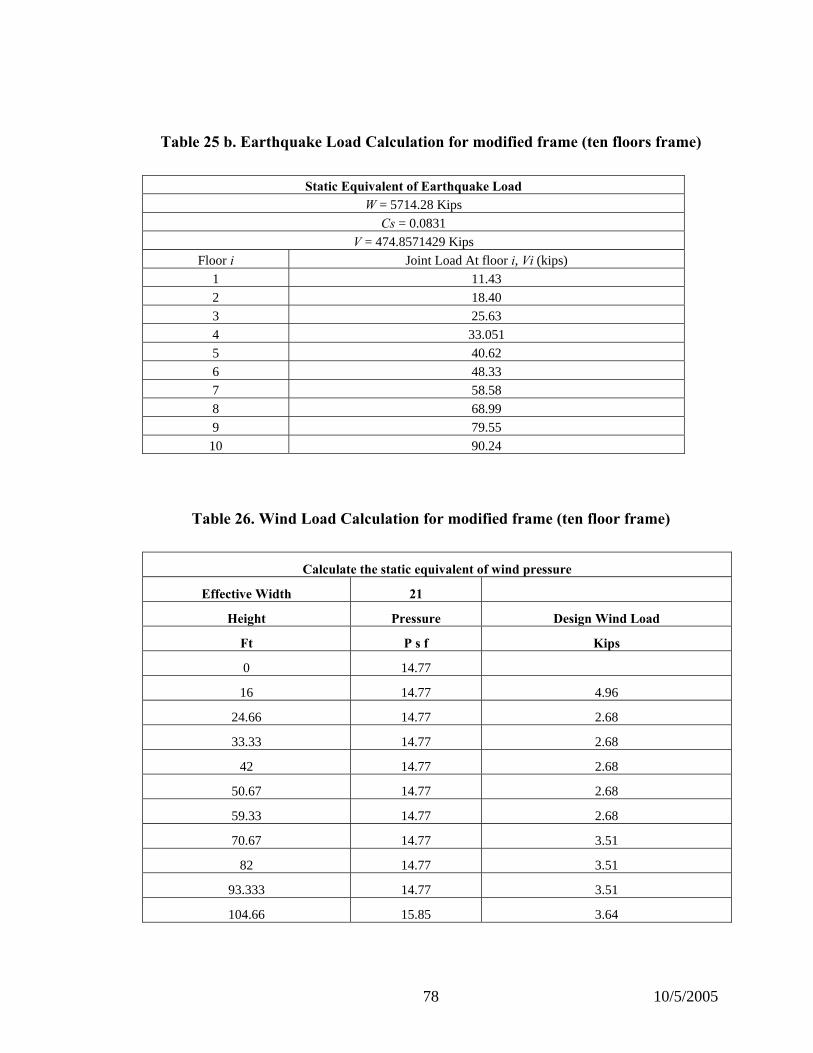
Table 25 b. Earthquake Load Calculation for modified frame (ten floors frame)
Static Equivalent of Earthquake Load W = 5714.28 Kips
Cs = 0.0831 V = 474.8571429 Kips
Floor i Joint Load At floor i, Vi (kips) 1 11.43 2 18.40 3 25.63 4 33.051 5 40.62 6 48.33 7 58.58 8 68.99 9 79.55
10 90.24
Table 26. Wind Load Calculation for modified frame (ten floor frame)
Calculate the static equivalent of wind pressure
Effective Width 21
Height Pressure Design Wind Load
Ft P s f Kips
0 14.77
16 14.77 4.96
24.66 14.77 2.68
33.33 14.77 2.68
42 14.77 2.68
50.67 14.77 2.68
59.33 14.77 2.68
70.67 14.77 3.51
82 14.77 3.51
93.333 14.77 3.51
104.66 15.85 3.64
10/5/2005 78

Table 27. Summary of Earthquake Load and Wind Load for modified frame (ten floors)
Summary of Loads
Dead Load U.D.L at all beam 18.2 kips/ft Live Load U.D.L at all beam 18 kips/ft
Earthquake Load Joint Load Wind Load Joint Load
Joint Height (ft) Earthquake Load
(kips) Wind Load (kips) 2 16 11.43 4.96 3 24.66 18.4 2.68 4 33.33 25.63 2.68 5 42 33.05 2.68 6 50.67 40.62 2.68 7 59.33 48.33 2.68 8 70.67 58.58 3.51 9 82 68.99 3.51
10 93.33 79.55 3.51 11 104.66 90.24 3.64
10/5/2005 79

62 65
Figure 8.1. Joints numbering for ten floors frame
68 77 59
58
60 63 66 69 72 75 57
16 24 32 40 48 56 8
7 55
6 54
5 53
4 52
1
2
3
49
50
51
9 17 25 33 41
11
10
10/5/2005 80

Figure 8.2. Frame elements numbering for ten floors frame
1
2
3
4
5
6
7
8 43
49
51 52 53 54 55
56
50
15 22 29 36
91 86
64
24
125 130
112
92
93
94
95
96
97
98
99
100
101
102
103
104
105
106
107
108
109
110
113 114 115 116 117 111 118
10/5/2005 81

8.1.1 Case 1- Maximum Span Moment of a Beam
Maximum span moment in a beam for the modified ten floors structure is the primary
focus of this subsection.
64
Figure 9.1. Case 1: Live load pattern for maximum span moment in beam – ten floors frame
10/5/2005 82

Table 28. Maximum Span Moment in beam 64(ten floor frame)
Beam 64 Interval Analysis Conventional Analysis
Load Combination Interval Span Moment (kips-inch) Maximum Span Moment (kips-inch)
1.4D [9297, 9297] 9297
1.2D+1.6L [7009, 19430] 19410
1.2D+L [7369, 15130] 15120
For the current ten-floor frame, span moments have been again evaluated using Interval
FE analysis and load pattern as shown in Figure 9.1. The first load combination (1.4D)
has the same lower and upper bound of interval span moment and it matched with what
load pattern has calculated. This is simply due to the fact that there is no live load pattern
involved. However, other two load combinations have different lower and upper bounds
of interval span moment (table 28) as they involve effect of live load pattern, maximum
span moment for load pattern in consideration is again within the interval.
8.1.2 Case 2- Minimum Span Moment of a Beam In this subsection interval finite element analysis is being compared with conventional
load pattern analysis through analyzing modified ten-frame structure for the minimum
span moments in the beam.
10/5/2005 83

64
Figure 9.2. Case 2: Live load pattern for minimum span moment in beam – ten-floor frame
Table 29. Minimum Span Moment in beam 64 (10 floor frame)
Beam 64 Interval Analysis Conventional Analysis
Load Combination Interval Span Moment (kips-inch) Minimum Span Moment (kips-inch)
1.4D [9297, 9297] 9297
1.2D+1.6L [7009, 19430] 7030
1.2D+L [7369, 15130] 7382
Interval FE analysis still hold the same result for ten-floor frame as far as span moment in
beam 64 is concerned as this analysis cover all the load pattern in itself by the nature of
10/5/2005 84

interval arithmetic however, engineer would like to consider a different load pattern for
analyzing the beam 64. Load pattern shown in Figure 9.2 is most general load pattern that
is being widely used in industry and also being suggested by various codes of practices
(see chapter for load combinations and load patterns), in this load pattern beam in
consideration is unloaded and every alternative beam is also unloaded. This will give
minimum span moment in beam under consideration and table 29 shows that this is
contained within interval span moment.
10/5/2005 85

8.1.3 Case 3 - Comparison for Maximum End Moments for Column 8
Once again, following three load patterns are being considered in order to get the
maximum and minimum end moments at the end of column. Column in which we are
interested is member 8.
Load Pattern A
8
Figure 9.3. Case 3: Live load pattern A for end moment at the end of column element – ten floors frame
10/5/2005 86

Table 30. End Moments in column 8 as an effect of Live Load Pattern A, B and C (ten-floor frame)
Interval Analysis Conventional Analysis
Load pattern A Load pattern B Load pattern C
Load Combination Interval End Moment
(Kips-inch)
End Moment
(Kips-inch)
End Moment
(Kips-inch)
End Moment
(Kips-inch)
1.4D [-1390.09, -1390.09] -1390.09 -1390.09 -1390.09
1.2D+1.6L [-12495.5, 8541.63] 4847.61 -8464.98 -11687.2
1.2D+L [-8256.52, 4891.7] 2582.94 -5737.43 -7751.31
1.2D+0.8W [-981.16, -981.16] -981.16 -981.16 -981.16
1.2 D + 1.6 W + L [-7835.82, 5312.4] 3003.64 -5316.73 -7330.61
1.2 D + 1.0 E1 + L [-4887.83, 8260.4] 5951.64 -2368.74 -4382.61
1.2 D + 1.0 E2 + L [-4857.24, 8290.98] 5982.22 -2338.15 -4352.03
0.9 D + 1.0 E1 [2450.04, 2450.04] 2450.04 2450.04 2450.04
0.9 D + 1.0 E2 [2505.64, 2505.64] 2505.64 2505.64 2505.64
0.9 D + 1.6 W [-472.932, -472.932] -472.932 -472.932 -472.932
Load factors as Interval [-15770.2, 15707.8]
10/5/2005 87

Live Load Pattern B
8
Figure 9.4. Case 3: Live load pattern B for end moment at the end of column– ten floors frame
10/5/2005 88

Live Load Pattern C
8
Figure 9.5. Case 3: Live load pattern C for end moment at the end of column– ten floors frame
It is important to note that in real practice analyzing a structure for three load pattern just
in order to get maximum or minimum end moment in one particular column may prove to
be a tiresome task and since using all possible load pattern for such cases are so
computation intensive and require enormous man time and computer time, it makes it
almost an impossible and impractical task.
10/5/2005 89

Table 22 shows that interval end moment width obtained in column 8 for every load
pattern and load combination is increasing (e.g. compare table 14 and 22) and it is not
difficult to show that it hold true for all the column and for all the structural parameter
like axial force, bending moment, axial force and then for every structural element as
beam or column. These results will be later explained in details in conclusion section.
8.2 Case B: Number of Floor = 15
1. Five floors have been added on the top of previously existing ten floors frame to
form a fifteen story portal frames.
2. Each of the added are of height 11 ft 4 inch.
3. Numbering of added joints and members is being in such a way so that joints and
members that we had in Case B, holds the same number, for the new ones,
column is being numbered first and then all remaining beams. This way there is a
minimal change to the input file.
4. Dead load and Live load for added floor is same as of previously existing floors.
5. Weight of the structure has been increased in proportion to number of floors.
6. Earthquake loads have been calculated based on IBC code of practices.
7. Wind load have been revised for modified structure using ASCE6 codes of
practices.
10/5/2005 90

Table 31 a. Earthquake load calculation for modified frame (fifteen floors frame)
Story Story Height Story Height from Base hi hik Cvx 1 16 16 21.11 0.01048 2 8.66 24.66 33.98 0.01688 3 8.66 33.33 47.33 0.02351 4 8.66 42 61.03 0.03031 5 8.66 50.66 75.02 0.03726 6 8.66 59.33 89.25 0.04433 7 11.33 70.66 108.17 0.05373 8 11.33 82 127.40 0.0632 9 11.33 93.33 146.90 0.07297
10 11.33 104.66 166.64 0.0827 11 11.33 116 186.59 0.09269 12 11.33 127.33 206.74 0.10270 13 11.33 138.66 227.07 0.11279 14 11.33 150 247.57 0.12298 15 11.33 161.33 268.22 0.1332
Total 2013.09
Table 31 b. Earthquake load calculation for modified frame (fifteen floor frame)
Static Equivalent of Earthquake Load
W = 8571.428571 Kips Cs = 0.0831
V = 712.2857143 Kips Floor i Joint Load At floor i, Vi (kips)
1 7.47 2 12.02 3 16.74 4 21.59 5 26.54 6 31.58 7 38.27 8 45.08 9 51.97
10 58.96 11 66.02 12 73.15 13 80.34 14 87.59 15 94.90
10/5/2005 91

Table 32. Wind load calculation for modified frame (fifteen floor frame) Calculate the static equivalent of wind pressure
Effective Width 21 Height Pressure Design Wind Load
Ft P s f Kips 0 14.77
16 14.77 4.961 24.66 14.77 2.687 33.33 14.77 2.687
42 14.77 2.687 50.66 14.77 2.687 59.33 14.77 2.687 70.66 14.77 3.514
82 14.77 3.514 93.33 14.77 3.514
104.66 15.85 3.643 116 15.85 3.773
127.33 16.94 3.902 138.66 16.94 4.031
150 17.81 4.134 161.33 18.68 4.341
Table 33. Summary of Earthquake load and Wind load for modified frame (fifteen
floor frame) Summary of Loads
Dead Load U.D.L at all beam 18.2 kips/ft Live Load U.D.L at all beam 18 kips/ft
Earthquake and wind Load Joint Load Joint Height (ft) Earthquake Load (kips) Wind Load (kips)
2 16 7.47 4.961 3 24.66 12.02 2.687 4 33.33 16.74 2.687 5 42 21.59 2.687 6 50.67 26.54 2.687 7 59.33 31.58 2.687 8 70.67 38.27 3.514 9 82 45.08 3.514
10 93.33 51.97 3.514 11 104.66 58.96 3.643 12 104.66 66.02 3.773 13 104.66 73.15 3.902 14 104.66 80.34 4.031 15 104.66 87.59 4.1349 16 104.66 94.9 4.341
10/5/2005 92

Figure 10.1. Joints numbering for fifteen-floor portal frame
1
2
3
4
5
6
7
8
6862 71 74 6559 77
78
79
80
81
82
83 88 93 98 103108
87 92 97 102 107 112
111
110
109
58
7260 63 66 69 75 57
24 40 4816 3256
55
54
53
52
49
50
51
9 17 25 33 41
11
10
10/5/2005 93

Figure 10.2. Frame elements numbering for fifteen floor frame
1
2
3
4
5
6
7
8 43
49
51 52 53 54 55
56
50
15 22 29 36
91 86
64
24
92
93
94
95
96
97
98
99
100
101
102
103
104
105
106
107
108
109
110
112
113 111 118
171
130
190 191 192 193 194 195
165 135 140 145
131
132
133
134
166 167 168
164
163
169 170 162
125 127 161
10/5/2005 94

8.2.1 Case 1 - Maximum Span Moment for Beam
am 64, first through
Figure 11.1. Case 1: live load pattern for aximum span moment in beam– fifteen- floor frame
In this section maximum span moment is being calculated in a be
interval FE analysis for 3 load combinations and then same member will be analyzed for
the load pattern shown in Figure 11.1.
64
m
10/5/2005 95

A
e)
Beam 64 lysis
s before this time again a load pattern that is conventionally being used for maximizing
span moment in beams, will be considered (Figure 11.2). Note that interval width has
increased as compared to what was obtained in seven floor or ten floor cases in earlier
sections (Table 10, 18 and 26). This is because of the fact that Interval FE analysis of
fifteen-floor frame covers 290 load patterns while seven and ten floor had 242 and 260
hence it cause lower and upper limit of span moment to deviate. However, maximum
span moment from conventional analysis can deviate in either way depending upon the
ratio of dead load and live load. In later part of work it will be shown about how the
maximum and minimum values of parameters such as span moment or end moment in a
member deviate from lower and upper limit of corresponding interval value.
Table 34. Maximum span moment in beam 64 (fifteen floors fram
Interval Analysis Conventional Ana
Load tion Interval s-inch) Maxim nch) Combina Span Moment (kip um Span Moment (kips-i
1.4D [9293, 9293] 9293
1.2 L D+1.6 [6991, 19440] 19410
1.2D+L [7356, 15140] 15120
8.2.2 Case 2 - Minimum Span Moment for Beam
at cause minimum span moment in
Same frame has been analyzed for load pattern th
beam. Same beam element has been picked up for the minimum span moment and only
three load combinations have been picked up.
10/5/2005 96

64
Figure 11.2. Case 2: Live load pattern for minimum span moment in beam element – fifteen floors frame
It is important to note that results from interval FE analysis contain the results from
conventional analysis but difference between maximum span moment and upper limit of
interval span moment (Table 26) or minimum span moment and lower limit of interval
span moment (Table 27) is not significant enough, this is the reason that efforts has not
10/5/2005 97

been put for analysis of all the 10 load combination, however column end moment show
a significant difference in this regard and hence in such cases results from all the 10 load
combinations are being used.
Table 35. Minimum span moment in beam 64 (fifteen floor frame)
Beam 64 Interval Analysis Conventional Analysis
Load Combination Interval Span Moment (kips-inch) Minimum Span Moment (kips-inch)
1.4D [9293, 9293] 9293
1.2D+1.6L [6991, 19440] 7025
1.2D+L [7356, 15140] 7378
10/5/2005 98

8.2.3 Case 3 - Comparison for End Moments in Column 8
In this case maximum and minimum end moments in column 8 are design parameters.
Three live load patterns will be taken into consideration in order to analyze column
conventionally. Figure 11.3, 11.4 and 11.5 shows live load pattern A, B and C.
8
Figure 11.3. Case 3: Live load pattern A for maximum/minimum end moment in column– fifteen-floor frame
10/5/2005 99

Results from Interval FE Analysis will then be compared for upper and lower bound of
interval end moments obtained from these three load patterns.
8
Figure 11.4. Case 3: Live load pattern B for maximum/minimum end moment in column– fifteen-floor frame
10/5/2005 100

Table 36. End Moment in Column 8 as per effect of Live Load Pattern A, B and C (fifteen floor frame)
Column 8 Interval Analysis Conventional Analysis
Load Pattern A Load Pattern B Load Pattern C
Load Combination Interval End Moment
(Kips-inch)
End Moment
(Kips-inch)
End Moment
(Kips-inch)
End Moment
(Kips-inch)
1.4D [-1542.88, -1542.88] -1542.88 -1542.88 -1542.88
1.2D+1.6L [-12968, 8579.49] 4715.4 -8662.33 -11923.8
1.2D+L [-8600.9, 4866.26] 2451.2 -5909.88 -7948.28
1.2D+0.8W [-1000.84, -1000.84] -1000.84 -1000.84 -1000.84
1.2 D + 1.6 W + L [-7957.64, 5509.52] 3094.46 -5266.62 -7305.02
1.2 D + 1.0 E1 + L [-3647.8, 9819.36] 7404.3 -956.777 -2995.18
1.2 D + 1.0 E2 + L [-3613.85, 9853.3] 7438.25 -922.833 -2961.23
0.9 D + 1.0 E1 [3933.48, 3933.48] 3933.48 3933.48 3933.48
0.9 D + 1.0 E2 [3995.19, 3995.19] 3995.19 3995.19 3995.19
0.9 D + 1.6 W [-348.592, -348.592] -348.592 -348.592 -348.592
Load factors as Interval [-16317.8, 17639]
10/5/2005 101

8
Figure 11.5. Case 3: Live load pattern C for maximum/minimum end moment in column– fifteen-floor frame
Results obtained from three conventional load patterns analysis and their comparison
with interval FE analysis has been explained in details in subsequent section. However,
all the results obtained until this point clearly shows that interval analysis guarantee to
contain the results from all possible load pattern and it hold equally valid for all type of
10/5/2005 102

load combinations. How close conventional analysis results can lie to the lower or upper
bound of interval results is still a moot point as exact nature of deviation of conventional
results from the bound of interval response, will depend on the type of load combination,
ratio of dead load to live load, ratio of horizontal to vertical forces and on structural
member properties itself. However, in next chapter efforts have been made in order to
study the nature of such deviations.
10/5/2005 103

9. DISCUSSION
In this section, results from all previous Interval FE Analysis and various conventional
load pattern analysis that had already been done, will be studied in detail. Table 31 focus
on beam element (beam 64), in the column A of table 31, interval span moments are
being listed for three load combinations and for three type of frames, seven floors, ten
floors and fifteen floors frame. First of all it is interesting to see that lower bound of
interval span moment decreases and at the same time upper bound increase numbers of
floors are increased. It happened because of the fact of increase in live load pattern that
Interval FE analysis is accounting for.
Table 37. Beam 64: Percentage deviation Vs number of floor
Beam 64 Column A Column B Column C
Interval FE Analysis Conventional Analysis % Deviation
Com
pari
son
for
Span
Mom
ent
Floors Interval FE Span
Moment Minimum Maximum Maximum Minimum 7 [7016, 19420] 7028 19410 0.05152 0.170746
10 [7009, 19430] 7030 19410 0.10304 0.29872 15 [6991, 19440] 7025 19410 0.15456 0.483986 Lo
ad C
ombi
natio
n
1.
2D +
1.6
L
7 [7373, 15130] 7380 15120 0.066138 0.094851
10 [7369, 15130] 7382 15120 0.066138 0.176104 15 [7356, 15140] 7378 15120 0.132275 0.298184 Lo
ad C
ombi
natio
n
1.
2D +
L
10/5/2005 104

Column B of table 31 lists the minimum and maximum span moment obtained from two
typical load patterns (refer to earlier sections for details). Column C of table 31 shows
percentage deviation of maximum span moment obtained from conventional analysis
with upper bound on interval span moment. This percentage deviation in this particular
case (beam 64) is not significant, however Figure 12a and 12b shows that this deviation is
increasing as number of floors are increased, in fact for almost all the load combination
that have been listed in table 31, this deviation build up to 300% as we increase number
of floor from 7 to 15.
Interval FE Analysis Vs Conventional Analysis
Span moment in beam 64
0
0.1
0.2
0.3
0.4
0.5
0.6
4 6 8 10 12 14 16
NO OF FLOORS
(INTR
VL-C
ON
VN)*
100/
CO
NVN
1.2D+1.6L - MAX
1.2D+1.6L - MIN
Figure 12a. Maximum and Minimum Span Moment in Beam 64 - Percentage deviation Vs number of floor for load combination 1.2 D + 1.6 L
10/5/2005 105

Interval FE Analysis Vs Conventional AnalysisSpan moment in beam 64
0
0.05
0.1
0.15
0.2
0.25
0.3
0.35
4 6 8 10 12 14 16
NO OF FLOORS
(INTR
VL-C
ON
VN)*
100/
CO
NVN
1.2D+L - MAX
1.2D+L - MIN
Figure 12b. Maximum and Minimum Span Moment in Beam 64 - Percentage
deviation Vs number of floor for load combination 1.2 D + L
10/5/2005 106

Table 38. Column 8: (Interval result – Conventional Result)*100/ Conventional Result Vs number of floor
Comparison of Upper & Lower Bounds from Interval FE Analysis with corresponding Max & Min values for End Moment from Conventional Analysis
Column 8 Interval FE Analysis Conventional Analysis Max +ve/-ve End Moment from Load Patterns
% Deviation
Cpa
riso
n fo
r M
axim
um E
nd
Mom
ent
om
Floors Interval End Moment
Load Pattern
A
Load Pattern
B
Load Pattern
C Maximum +ve Maximum –ve Max +ve Max -
ve 7 [-12193.5, 8515.77] 4927.87 -8307.41 -11568.9 4927.87 -11568.9 72.80 5.39
10 [-12495.5, 8541.63] 4847.61 -8464.98 -11687.2 4847.61 -11687.2 76.20 6.9115 [-12968, 8579.49] 4715.4 -8662.33 -11923.8 4715.4 -11923.8 81.94 8.75
Lad
C
ombi
natio
n
1.2D
+ 1
.6L
o
7 [-7730.38, 5212.92] 2970.49 -5301.56 -7339.97 2970.49 -7339.97 75.49 5.31
10 [-7835.82, 5312.4] 3003.64 -5316.73 -7330.61 3003.64 -7330.61 76.86 6.8915 [-7957.64, 5509.52] 3094.46 -5266.62 -7305.02 3094.46 -7305.02 78.04 8.93
Lad
C
ombi
natio
n
1.
2D +
L +
1.6
W
o
7 [-5563.06, 7380.24] 5137.8 -3134.25 -5172.65 5137.8 -5172.65 43.64 7.54
10 [-4857.24, 8290.98] 5982.22 -2338.15 -4352.03 5982.22 -4352.03 38.59 11.6015 [-3613.85, 9853.3] 7438.25 -922.833 -2961.23 7438.25 -2961.23 32.46 22.03
Lad
C
ombi
natio
n
1.
2D +
L +
E2
o
10/5/2005 107

Comparison of Upper & Lower Bounds from Interval FE Analysis with corresponding Max & Min values for End Moment from Conventional Analysis
Column 8 Interval FE Analysis Conventional Analysis Max +ve/-ve End Moment from Load Patterns
% Deviation
Cpa
riso
n fo
r xi
mum
End
M
om
om
ent
Ma
Floors Interval End Moment
Load Pattern
A
Load Pattern
B
Load Pattern
C Maximum +ve Maximum -ve Max +ve Max -
ve 7 [-5591.51, 7351.79] 5109.36 -3162.69 -5201.09 5109.36 -5201.09 43.88 7.50
10 [-4887.83, 8260.4] 5951.64 -2368.74 -4352.03 5951.64 -4382.61 39.30 10.8315 [-3647.8, 9819.36] 7404.3 -956.777 -2995.18 7404.3 -2995.18 32.61 21.78
Load
Cbi
natio
n
1.2D
+ L
1
om
+ E
10/5/2005 108

However, these trends become dominant when results obtained from column 8 are
studied. Table 32 lists down interval end moment and end moment obtained from three
different load pattern. In previous sections, results are shown for ten load combination,
however for the time being only these four load combinations have been extracted as
these are the best representative of all the load combinations in order to show the
capability of Interval FE Analysis.
Once again interval end moment width increases as we increase number of floors. For
load combination 1.4 D + 1.6 L deviation of maximum positive end moment from upper
bound of interval end moment is quite significant, for seven floor frame it is about 72%,
this indicate the fact that at times conventional structural analysis may prove to be very
underestimating and results can be drastically wrong.
Interval FE Analysis Vs Conventional AnalysisEnd moments in column 8
0
10
20
30
40
50
60
70
80
90
5 7 9 11 13 15 17
Number of Floor
(INTR
VL-C
ON
V)*1
00/C
ON
V
1.2D+1.6L & Max +ve EndMoment
1.2D+1.6L & Max -ve EndMoment
Figure 13a. Bounds on End Moment in Column 8- Percentage Deviation Vs number of floor for load combination 1.2D+1.6L
10/5/2005 109

Interval FE Analysis Vs Conventional AnalysisEnd moments in column 8
0
10
20
30
40
50
60
70
80
90
5 7 9 11 13 15 17
Number of Floor
(INTR
VL-C
ON
V)*1
00/C
ON
V
1.2D+1.0L+1.6W & Max +veEnd Moment
1.2D+1.0L+1.6W & Max -veEnd Moment
Figure 13b. Bounds on End Moment in Column 8- Percentage Vs number of floor for load combination 1.2D+1.0L+1.6W
Interval FE Analysis Vs Conventional AnalysisEnd moments in column 8
0
5
10
15
20
25
30
35
40
45
50
5 7 9 11 13 15 17
Number of Floor
(INTR
VL-C
ON
V)*1
00/C
ON
V
1.2D+1.0E2+L & Max +ve EndMoment
1.2D+1.9E2+L & Max -ve EndMoment
Figure 13c. Bounds on End Moment in Column 8- Percentage Deviation Vs number of floor for load combination 1.2D+1.0E2+L
10/5/2005 110

In this specific example the deviation of conventional result from interval bounds for end
moment in column 8, does not build up to that extent as it was for beam element 64.
Table 32 shows that for 1.2D+1.6L, deviation grow up from 72.8% only up to 81.9% as
we move from seven-story frame to fifteen-story frame. For the load combination
1.2D+L+E2 and seven story frame, maximum negative end moment is about 7% of lower
bound of interval end moment, and it grow up to 22% as we move to fifteen floor frame.
However, for the same combination 1.2D+L+E2, deviation of maximum end moment
from upper bound of interval end moment drops from 43% to 32.5%, and such drops can
be attributed to the nature of earthquake load involved in the load combination, however
it is important to note that in situations where it deviate a lot, safety of structure is
potentially threatening.
Additionally it is interesting to see that in order to capture exact critical scenario, interval
FE analysis need only one interval run instead of running several load pattern. This can
be verified as all the tables presented so far clearly show that the results obtained from
conventional load pattern is strictly in between the lower and upper bounds of interval
response. At the same time interval response will guarantee the enclosure of exact
response within the sharp interval bounds. This kind of guarantee can never be assured by
analyzing structure for few selected load patterns. Since interval response always contain
all conventional structural analysis result that at times engineer would not even think to
consider just because of the time and efforts needed, this is the most efficient and easiest
approach available so far in order to find critical scenario for large and complicated real
structures. Adoption of this technique in real analysis and design work will make life of
10/5/2005 111

an engineer a lot simpler and hence will help them in ensuring safety of large-scale
structures.
10/5/2005 112

10. Conclusions
The presented work shows that structural response obtained from interval finite element
analysis bounds the structural response from conventional structural analysis for all
possible load patterns. Load combinations that don’t involve the presence of live load
result in analyses that are identical as far as these two procedures (Interval finite element
analysis and conventional load pattern analysis) are concerned. This is due to the fact that
in such cases loads are considered completely deterministic and each method corresponds
to one structural analysis iteration.
However due to presence of live load, a number of live load patterns come into picture
and multiple analyses are needed. Since interval loads can capture all the combinations of
presence and absence of individual load, interval finite element analysis gives a lower
and upper bound on the structural response.
The difference between lower and upper bound can be related to the number of possible
live load patterns. As we increase the number of floors in a frame, the numbers of load
patterns also increases. In the current thesis work, it has been verified that the width of
interval increases as we increase number of floors.
The structural response obtained from a few selected live load patterns is not necessarily
a critical scenario for all the design parameters that an engineer may need in a design.
Thus, unless a complete load pattern analysis is done, the critical response predicted
through such load patterns can vary significantly from the actual critical response.
However the lower or/and upper bound of interval response if used in design practices,
10/5/2005 113

will ensure that correct values of all the design parameters are used. In such cases, design
will be more accurate and economic.
The deviation of conventional load pattern analysis results from the bounds of interval
response is independent of structural element type. It does not make any difference which
structural element is picked up as the design element.
Additionally all the structural parameters like span moments, end moments, shear force,
axial force and joint displacements can be evaluated for lower and upper bounds through
interval finite element analysis. Since all the parameters obtained in one run show
interval enclosure on all the critical scenarios obtained from different load pattern
analysis, interval finite element analysis proves to be very efficient as compared to
conventional load pattern analysis.
Interval finite element analysis provides a way to combine all the load patterns and load
combinations through interval load factors and interval load. In current thesis work
results obtained using interval load factors and interval loads are highly conservative as
interval load factors has been formulated in a crude way. A more complex formulation
for interval load factors would result in a much sharper interval response.
10/5/2005 114

APPENDIX A
Here is the computer program written in C++ for analyzing a portal frame under joint
load and continuous loads and for load combination using interval finite element
technique. Chapter 6 discusses this program in details. Here is the computer code
attached.
//Load Combination Frame finite element program //use conventional FEM formula for BASIC //LOAD: interval nodal load and element uniform load //use PROFIL to solve the system equation // by Dr. Rafi Muhanna / Hao Zhang / Vishal Saxena // June 25, 2002 #include "intmat.h" #include "util.cpp" #include "func.h" #include <iostream.h> #include <fstream.h> #include <stdio.h> #include <math.h> class FRAME { protected: int NELE;//number of elements int NNOD;//number of nodes char* filename;//the inputdata filename MATRIX mNode_info; //node information, store:node number,support information,x and y coordinates //MATRIX mEleInfo;//element connectivity and element uniform load,store: ele number, connectivity, and uniform distribute load( positive, if the element direction counterclockwize 90 to the uniform load direction) MATRIX mEleInfo;//element connectivity //MATRIX mNodalLoad;//nodal external load, store: x,y and theta 3 terms repectively //Dead Load INTERVAL_VECTOR ivEleLoadDL;//element load,in our program, only interval uniform load are allowed //Live Load INTERVAL_VECTOR ivEleLoadLL;//element load,in our program, only interval uniform load are allowed
10/5/2005 115

//Earthquake Load : EQ coming from one direction INTERVAL_MATRIX imNodalLoadEL;//interval nodal load, x y and theta //Wind Load INTERVAL_MATRIX imNodalLoadWL;//interval nodal load, x y and theta //Load factor INTERVAL_VECTOR loadFactor ; INTERVAL_VECTOR ivPc;//assembled system nodal load,only include the external loadal load INTEGER_MATRIX IBOU;//record boundary conditions, 0:fixed, 1: free MATRIX GSTF; MATRIX mMaterial;//material, include: A,I and E MATRIX mMatrix;//m matrix MATRIX mMatrix_noBC;//m matrix without BC imposed, used in element force calculation INTERVAL_VECTOR ivDisplacement;//nodal displacement INTERVAL_VECTOR LOAD_EBE_expand;//nodal load, assembled by imPc public: FRAME(); void InitialData();//used in constructor void ReadData(); void Boundary();//construct IBOU,used in Calculation() void Calculation();//assemble GSTF, calculate displacement, and element internal forces void ElementForce();//calculate element force MATRIX Estf_Calculation( int );//this function return the element stiffness MATRIX M_Matrix_Calculation(); }; FRAME::FRAME() { filename=new char[100]; InitialData(); Resize(mNode_info,NNOD,6);//stor the node number,support infor, x coordinate and y coordinate Clear (mNode_info); Resize(mEleInfo,NELE,3);//store the ele #, connectivity Clear (mEleInfo); Resize (mMaterial,NELE,3);//store the A,I,E Clear (mMaterial); Resize (ivEleLoadDL,NELE);//store the interval dead load terms on x,y,theta dofs, respectively Clear (ivEleLoadDL);
10/5/2005 116

Resize (ivEleLoadLL,NELE);//store the interval live load terms on x,y,theta dofs, respectively Clear (ivEleLoadLL); Resize (imNodalLoadEL,NNOD,3);//store the interval earthquake load terms on x,y,theta dofs, respectively Clear (imNodalLoadEL); Resize (imNodalLoadWL,NNOD,3);//store the interval wind load terms on x,y,theta dofs, respectively Clear (imNodalLoadWL); Resize(loadFactor,4); Clear(loadFactor); Resize (ivPc,NNOD*3); Clear (ivPc); Resize (GSTF,NNOD*3,NNOD*3); Clear (GSTF); Resize (mMatrix,NNOD*3,NELE); Clear (mMatrix); Resize (mMatrix_noBC,NNOD*3,NELE); Clear (mMatrix_noBC); Resize (IBOU,NNOD,3); Clear (IBOU); } void FRAME::InitialData() { fstream INFILE; char *string=new char[80]; cout<<"please specify the input data filename."<<endl; scanf("%s",filename); INFILE.open(filename,ios::in|ios::nocreate,1); if (! INFILE){//in case the mistyped data file name cout<<"Data file does not exit! program terminated, please try later!"<<endl; exit(0); } INFILE.getline(string,80);
10/5/2005 117

INFILE.getline(string,80); INFILE >> NNOD>>NELE;//number of elements,number of nodes INFILE.close(); } void FRAME::ReadData() { fstream INFILE; INFILE.open(filename,ios::in,1); char *string=new char[180]; INFILE.getline(string,180);//eliminate the first comment line INFILE.getline(string,180); INFILE >> NNOD; INFILE >> NELE; INFILE.getline(string,180); INFILE.getline(string,180); INFILE >> mNode_info; INFILE.getline(string,180); INFILE.getline(string,180); INFILE >> mEleInfo; INFILE.getline(string,180); INFILE.getline(string,180); INFILE >>mMaterial; //Dead Load Information INFILE.getline(string,180); INFILE.getline(string,180); INFILE >>ivEleLoadDL; //Live Load Information INFILE.getline(string,180); INFILE.getline(string,180); INFILE >>ivEleLoadLL; //Earthquake Load Information INFILE.getline(string,180); INFILE.getline(string,180); INFILE >>imNodalLoadEL; //Wind Load Information INFILE.getline(string,180); INFILE.getline(string,180); INFILE >>imNodalLoadWL; //Load Factor Information INFILE.getline(string,180); INFILE.getline(string,180); INFILE >>loadFactor; INFILE.close();
10/5/2005 118

} void FRAME::Boundary() { Clear (IBOU); for (int i=1;i<=NNOD;i++) for (int j=1;j<=3;j++) IBOU(i,j)=int (mNode_info(i,j+1)); } MATRIX FRAME::Estf_Calculation(int IE) { VECTOR vQie(6); MATRIX ESTF(6,6); MATRIX ESTT(6,6); Clear (ESTT); Clear (ESTF); int I1= int(mEleInfo(IE,2)); int I2= int(mEleInfo(IE,3)); double X1= mNode_info(I1,5); double Y1= mNode_info(I1,6); double X2= mNode_info(I2,5); double Y2= mNode_info(I2,6); double AL= Sqrt(Sqr(X2-X1) + Sqr(Y2-Y1)); double AA = mMaterial(IE,1);// material const: A (area of the element) double AI = mMaterial(IE,2);//material const: I (moment of inertia) double AE = mMaterial(IE,3);///material const: E (elastic modulus) ESTF(1, 1) = AA*AE/AL; ESTF(4, 1) = - ESTF(1, 1); ESTF(2, 2) = 12.0*AE*AI/(AL*AL*AL); ESTF(3, 2) = 6.0*AE*AI/(AL*AL); ESTF(4, 2) = 0.0; ESTF(5, 2) = -ESTF(2, 2); ESTF(6, 2) = ESTF(3, 2); ESTF(3, 3) = 4.0*AE*AI/AL; ESTF(5, 3) = -ESTF(3, 2); ESTF(6, 3) = ESTF(3, 3)/2.0; ESTF(4, 4) = ESTF(1, 1); ESTF(5, 5) = ESTF(2, 2); ESTF(6, 5) = ESTF(5, 3); ESTF(6, 6) = ESTF(3, 3);
10/5/2005 119

//calculate the element stiffness, 6x6,beam element, see the fomula of structural mechanics PP317 int k=1; for (int i = 1;i <= 6; i++,k++){ for(int j= k; j <= 6; j++) ESTF(i, j) = ESTF (j, i); } //symetric element stiffness double CO = (X2-X1)/AL; double SI = (Y2-Y1)/AL; MATRIX T (6,6); Clear (T); T(1, 1) = CO; T(2, 1) = -SI; T(1, 2) = SI; T(2, 2) = CO; T(3, 3) = 1.0; T(4, 4) = CO; T(5, 4) = -SI; T(4, 5) = SI; T(5, 4) = -SI; T(4, 5) = SI; T(5, 5) = CO; T(6, 6) = 1.0;//calculate the transformation matrix ESTT = Transpose(T) * ESTF * T; vQie(1)=vQie(4)=0.; vQie(2)=vQie(5)=AL/2; vQie(3)=AL*AL/12; vQie(6)=-AL*AL/12; INTEGER_MATRIX IBOU_ELE (2, 3); Clear (IBOU_ELE); for ( int j=1;j<=3;j++){ IBOU_ELE(1,j)=IBOU(I1,j); IBOU_ELE(2,j)=IBOU(I2,j); } vQie=Transpose(T)*vQie; for (i=1;i<=3;i++){ mMatrix_noBC((I1-1)*3+i,IE)=vQie(i); mMatrix_noBC((I2-1)*3+i,IE)=vQie(i+3); }
10/5/2005 120

vQie=T*vQie; for (i=1;i<=2;i++) for (int j=1;j<=3;j++) if (0==IBOU_ELE(i,j)) vQie((i-1)*3+j) = 0.; vQie=Transpose(T)*vQie; for (i=1;i<=3;i++){ mMatrix((I1-1)*3+i,IE)=vQie(i); mMatrix((I2-1)*3+i,IE)=vQie(i+3); } return ESTT; } void FRAME::Calculation() { //here to get the material information //here to get the nodal load information int NDOF = 3 * NNOD; VECTOR vP(NDOF); Clear (vP); //system stiffness matrix //now do element loop, to calculate the element stiffness->assembly to system stiffness matrix; for (int IE=1;IE<=NELE;IE++){ MATRIX ESTT(6,6); ESTT = Estf_Calculation(IE); //========================================================================== // Assembling the Global Stiffness Matrix, and load vector vP int I1= int(mEleInfo(IE,2)); int I2= int(mEleInfo(IE,3)); INTEGER_VECTOR LM(6); Clear (LM); for (int I=1;I<=3;I++){ LM(I)=I + 3*I1-3; LM(I+3)= I + 3*I2-3; } for (I=1;I<=6;I++){ int NN= LM(I); //vP(NN)+=Pe(I); for (int J=1;J<=6;J++){ int MM=LM(J); GSTF(NN,MM)+=ESTT(I,J); } } }//the end of element loop, here we get GSTF
10/5/2005 121

//Next to introduce BC in GSTF to eliminat the singularity of GSTF // rows and columns corresponding // to the restrained ith DOF are zeros, GSTF(i,i)=1 for (int I=1;I<=NNOD;I++){ for (int J=1;J<=3;J++){ int MM=IBOU(I,J); if (0==MM){ int K=3*I-3+J; for (int mm=1; mm<=NDOF;mm++){ GSTF(mm,K)=0.; GSTF(K,mm)=0.; } GSTF(K,K)=1.; } } } INTERVAL_VECTOR U(NDOF); INTERVAL_VECTOR U1(NDOF); INTERVAL_VECTOR U2(NDOF); for (int i=1;i<=NNOD;i++){ for (int j=1;j<=3;j++){ int NN=(i-1)*3+j; int MM=IBOU(i,j); ivPc(NN)=loadFactor(2)*imNodalLoadEL(i,j)+loadFactor(4)*imNodalLoadWL(I ,j); if(0==MM){ ivPc(NN)=0.;//assemble nodal load } } } //now we have GSTF and ivPc,and introduced BC, next , to get displacement // COMPUTATION OF SYSTEM DISPLACEMENTS //U=Inverse(GSTF)*(ivPc+mMatrix*ivEleLoadLL);//have overestimation??!! U1=Inverse(GSTF)*ivPc; U2=Inverse(GSTF)*mMatrix*(loadFactor(1)*ivEleLoadDL+loadFactor(3)*ivEle LoadLL); U=U1+U2; //Displacement for current Load Combination
10/5/2005 122

fstream Uoutput; Uoutput.open("U-ISA-OUT.TESTEX2.txt",ios::out,1); Uoutput<<"now output the interval nodal displacement."<<endl; for (int IN=1;IN<=NNOD;IN++){ Uoutput<<"Node: "<<IN<<" "; for ( int i=1;i<=3;i++) Uoutput<<U((IN-1)*3+i)<<" " ; Uoutput<<endl; } Uoutput.close(); } void FRAME::ElementForce() { int NDOF = 3 * NNOD; //Added by Vishal Saxena : 07/05/2003 //Parameters used in order to compute maximum Bending Moment within the span of beam - Start MATRIX EL(6,NELE); VECTOR R1(NELE); VECTOR R2(NELE); VECTOR R3(NELE); VECTOR R4(NELE); VECTOR R5(NELE); REAL dist; REAL D; INTERVAL max, max1, max2; //Parameters used in order to compute maximum Bending Moment within the span of beam - End fstream Feoutput; Feoutput.open("F-ISA-OUT.TESTEX2.txt",ios::out,1); Feoutput<<"now output the interval element interval force"<<endl; for (int IE=1;IE<=NELE;IE++){ //if(IE == 8 || IE == 64){ INTERVAL_VECTOR ivEF(6);//element force INTERVAL iEleLoad; iEleLoad=loadFactor(1)*ivEleLoadDL(IE)+loadFactor(3)*ivEleLoadLL(IE) ; int el=(iEleLoad!= 0)?1:0; int I1= int(mEleInfo(IE,2)); int I2= int(mEleInfo(IE,3));
10/5/2005 123

MATRIX mL(6,NDOF);//boolean matrix, mL*U=Ue Clear (mL); for (int i=1;i<=3;i++){ mL(i,(I1-1)*3+i)=1; mL(i+3,(I2-1)*3+i)=1; } //formula: see the structural mechanics book:P339, Fe=KeUe+Fp*/ ivEF=Estf_Calculation(IE)*mL*Inverse(GSTF)*ivPc+(Estf_Calculation(IE)*Ml *Inverse(GSTF)*mMatrixel*mL*mMatrix_noBC)*(loadFactor(1)*ivEleLoadDL +loadFactor(3)*ivEleLoadLL); EL = (Estf_Calculation(IE)*mL*Inverse(GSTF)*mMatrix- el*mL*mMatrix_noBC); R1 = Row(EL,2); R2 = Row(EL,3); dist = R1(IE); D = (dist * dist)/2.; R3 = dist * R1; Clear (R4); R4(IE)= D; R5 = R3 - R4; max1 = (R5 - R2) * (loadFactor(1)*ivEleLoadDL); max2 = (R5 - R2) * (loadFactor(3)*ivEleLoadLL); max = max1 + max2; Feoutput<<"ELEMENT # "<<IE<<endl; for (i=1;i<=6;i++){ Feoutput<<ivEF(i)<<" "; Feoutput<<endl; } Feoutput << " Max-Min-DS span moments = " << max <<endl; //} }//End of Element Loop Feoutput.close(); cout<<"Please see the results in the output file\n"; }
10/5/2005 124

int main() { FRAME* pFRAME=new FRAME(); pFRAME->ReadData(); pFRAME->Boundary(); pFRAME->Calculation(); pFRAME->ElementForce(); delete pFRAME; return 0; }
10/5/2005 125

REFERENCES
Alfred, G., and Herzberger, J. (1983). Introduction to interval computations. Academic,
New York.
Apostolatos, N., and Kulisch, U. (1968). “Grundzuge einer Intervallrechtung fur Matrizen
und einige Anwwendungen, Elektron. Rechenanlagen, 10, 73-83 (in German).
Bleher, J.H., Rump, S.M.,Kulisch, U.W., Metzer, M.Ullrich, Ch., and Walter, W.(1987).
“FORTRAN-SC: A study of a FORTRAN extension of engineering/scientific
computations with access to ACRITH.” Computing, 29, 93-110.
Building Code Requirements for Structural Concrete (ACI 318-02) and Commentary
(ACI 318R-02), American Concrete Institute, Farmington Hills, MI
Center of Reliable Computing, Georgia Tech Regional Engineering Program (GTREP)
Savannah.
Dwyer, P.S., ed.(1951). Computation with approximate numbers, linear computations,
Wiley, New York, 11-34.
Hansen, E. (1965). “Interval arithmetic in matrix computation.” SIAM J.,numer. Anal.,
19(4), 858-870
Hansen, E. (1992). Global optimization using interval analysis. Marcel Dekker, New
York.
International Building Code (2000), Chapter 16, Structural Design, International code
council.
Introductory Problems in Structural Analysis, an article accessible at
http://www.public.iastate.edu/~fanous/ce332/influence/homepage.html
10/5/2005 126

Jansson, C. (1991). “Interval linear system with symmetric Matrices, Skew-Symmetric
matrices, and dependencies in the right hand side.” Computing, 46, 265-274
Köyluoglu, H.U., Cakmak, A.S., and Nielsen, S.R.K. (1995). “Interval algebra to deal
with pattern loading and structural uncertainty Journal of Engineering
Mechanics., ASCE, 121(11), 1149-1157.
Köyluoglu, U., and Elishakoff, I. (1998). “A comparison of stochastic and interval finite
elements applied to shear frames with uncertain stiffness properties.” Comp. and
Struct., 67(1-3),91-98
Mayer, O. (1970). “Algebraische und metrrische Strunkturen in der Intervallrechung und
eingine Anwendungen.” Computing, 5, 144-162 (in German).
Minimum Design Loads for Buildings and Other Structures (ASCE7-2002),
American Society of Civil Engineers
Moor R.E.(1966). Interval analysis. Prentice-Hall, Englewood Cliffs, N.J.
Muhanna, R. L. and Mullen, R. L. (1995). “Development of interval based methods for
fuzziness in continuum mechanics.” Proc. ISUM A-NAFIPS ’95, IEEE Computer
Society Press, Los Alamos, Calif., 145-150.
Muhanna, R. L. and Mullen, R. L. (1999). “Formulation of fuzzy finite element methods
for mechanics problems.” J. Comp.-Aided Civ. And Infrastructure Engrg., 14,
107-117.
Mullen, R. L. and Muhanna, R. L. (1996). “Structural analysis with fuzzy-based load
uncertainty.” Proc., 7th ASCE EMD/STD Joint Spec. Conf. on Probabilistic Mech.
and Struct. Reliability, WP I,MA, ASCE, New York, 310-313
10/5/2005 127

Mullen, R. L. and Muhanna, R. L. (1999). “Bounds of Structural Response for All
Possible Loading Combinations”, Journal of Structural Engineering, Vol. 125,
No. 1, January 1999.
Neumaier, A. (1987). Interval methods for system of equations, Cambridge University
Press, New York.
Nilson, A.H., and Winter, G. (1991) “Design of concrete structures”, McGraw-Hill, New
York.
Rao, S.S., and Berke, L. (1997). “Analysis of uncertain structural systems using interval
analysis.” AIAA J., 35(4), 727-735
Rao, S.S., and Chen, Li. (1998). “Numerical solution of fuzzy linear equations in
engineering analysis.” Int. J. Numer. Methods in Engrg., 43, 391-408.
Rao, S.S., and Sawyer, P. (1995). “Fuzzy finite element approach for analysis of
imprecisely defined systems.” AIAA J., 33(12), 2364-2370
Sunaga, T. (1958). “Theory of interval algebra and its application to numerical analysis.”
RAAG Memoirs 3, 29-46
Uniform building code. (1998). International Conference of Building Officials, Whittier,
Calif., 126.
Zadeh, L.A. (1965). “Fuzzy sets.” Information and Control, 8, 338-353
10/5/2005 128

10/5/2005 129