scalable private learning with pate · pate approach multiple teachers are trained on disjoint...

Published as a conference paper at ICLR 2018

SCALABLE PRIVATE LEARNING WITH PATE

Nicolas Papernot∗Pennsylvania State [email protected]

Shuang Song∗University of California San [email protected]

Ilya Mironov, Ananth Raghunathan, Kunal Talwar & Úlfar ErlingssonGoogle Brain{mironov,pseudorandom,kunal,ulfar}@google.com

ABSTRACT

The rapid adoption of machine learning has increased concerns about the privacyimplications of machine learning models trained on sensitive data, such as medicalrecords or other personal information. To address those concerns, one promisingapproach is Private Aggregation of Teacher Ensembles, or PATE, which transfersto a “student” model the knowledge of an ensemble of “teacher” models, withintuitive privacy provided by training teachers on disjoint data and strong privacyguaranteed by noisy aggregation of teachers’ answers. However, PATE has so farbeen evaluated only on simple classification tasks like MNIST, leaving unclear itsutility when applied to larger-scale learning tasks and real-world datasets.In this work, we show how PATE can scale to learning tasks with large numbersof output classes and uncurated, imbalanced training data with errors. For this, weintroduce new noisy aggregation mechanisms for teacher ensembles that are moreselective and add less noise, and prove their tighter differential-privacy guarantees.Our new mechanisms build on two insights: the chance of teacher consensus isincreased by using more concentrated noise and, lacking consensus, no answerneed be given to a student. The consensus answers used are more likely to becorrect, offer better intuitive privacy, and incur lower-differential privacy cost. Ourevaluation shows our mechanisms improve on the original PATE on all measures,and scale to larger tasks with both high utility and very strong privacy (ε < 1.0).

1 INTRODUCTION

Many attractive applications of modern machine-learning techniques involve training models usinghighly sensitive data. For example, models trained on people’s personal messages or detailed med-ical information can offer invaluable insights into real-world language usage or the diagnoses andtreatment of human diseases (McMahan et al., 2017; Liu et al., 2017). A key challenge in suchapplications is to prevent models from revealing inappropriate details of the sensitive data—a non-trivial task, since models are known to implicitly memorize such details during training and also toinadvertently reveal them during inference (Zhang et al., 2017; Shokri et al., 2017).

Recently, two promising, new model-training approaches have offered the hope that practical, high-utility machine learning may be compatible with strong privacy-protection guarantees for sensitivetraining data (Abadi et al., 2017). This paper revisits one of these approaches, Private Aggrega-tion of Teacher Ensembles, or PATE (Papernot et al., 2017), and develops techniques that improveits scalability and practical applicability. PATE has the advantage of being able to learn from theaggregated consensus of separate “teacher” models trained on disjoint data, in a manner that bothprovides intuitive privacy guarantees and is agnostic to the underlying machine-learning techniques(cf. the approach of differentially-private stochastic gradient descent (Abadi et al., 2016)). In thePATE approach multiple teachers are trained on disjoint sensitive data (e.g., different users’ data),and uses the teachers’ aggregate consensus answers in a black-box fashion to supervise the trainingof a “student” model. By publishing only the student model (keeping the teachers private) and byadding carefully-calibrated Laplacian noise to the aggregate answers used to train the student, the

∗Equal contributions, authors ordered alphabetically. Work done while the authors were at Google Brain.

1

arX

iv:1

802.

0890

8v1

[st

at.M

L]

24

Feb

2018


0 1000 2000 3000 4000 5000 6000Number of queries answered

66

68

70

72

74

76

Stu

dent

test

acc

ura

cy (

%)

ε= 0.76

ε= 2.89

ε= 1.42

ε= 5.76

LNMax

Confident-GNMax


0

1

2

3

4

5

6

Pri

vacy

cost

ε a

t δ=

10−

8

LNMax

Confident-GNMax

0% 20% 40% 60% 80% 100%Percentage of teachers that agree

0

500

1000

1500

2000

2500

Num

ber

of

queri

es

answ

ere

d LNMax answers

Confident-GNMaxanswers

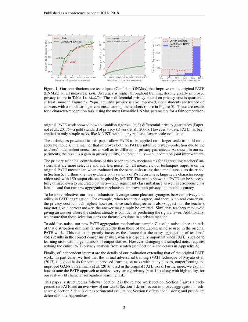
Figure 1: Our contributions are techniques (Confident-GNMax) that improve on the original PATE(LNMax) on all measures. Left: Accuracy is higher throughout training, despite greatly improvedprivacy (more in Table 1). Middle: The ε differential-privacy bound on privacy cost is quartered,at least (more in Figure 5). Right: Intuitive privacy is also improved, since students are trained onanswers with a much stronger consensus among the teachers (more in Figure 5). These are resultsfor a character-recognition task, using the most favorable LNMax parameters for a fair comparison.

original PATE work showed how to establish rigorous (ε, δ) differential-privacy guarantees (Paper-not et al., 2017)—a gold standard of privacy (Dwork et al., 2006). However, to date, PATE has beenapplied to only simple tasks, like MNIST, without any realistic, larger-scale evaluation.

The techniques presented in this paper allow PATE to be applied on a larger scale to build moreaccurate models, in a manner that improves both on PATE’s intuitive privacy-protection due to theteachers’ independent consensus as well as its differential-privacy guarantees. As shown in our ex-periments, the result is a gain in privacy, utility, and practicality—an uncommon joint improvement.

The primary technical contributions of this paper are new mechanisms for aggregating teachers’ an-swers that are more selective and add less noise. On all measures, our techniques improve on theoriginal PATE mechanism when evaluated on the same tasks using the same datasets, as describedin Section 5. Furthermore, we evaluate both variants of PATE on a new, large-scale character recog-nition task with 150 output classes, inspired by MNIST. The results show that PATE can be success-fully utilized even to uncurated datasets—with significant class imbalance as well as erroneous classlabels—and that our new aggregation mechanisms improve both privacy and model accuracy.

To be more selective, our new mechanisms leverage some pleasant synergies between privacy andutility in PATE aggregation. For example, when teachers disagree, and there is no real consensus,the privacy cost is much higher; however, since such disagreement also suggest that the teachersmay not give a correct answer, the answer may simply be omitted. Similarly, teachers may avoidgiving an answer where the student already is confidently predicting the right answer. Additionally,we ensure that these selection steps are themselves done in a private manner.

To add less noise, our new PATE aggregation mechanisms sample Gaussian noise, since the tailsof that distribution diminish far more rapidly than those of the Laplacian noise used in the originalPATE work. This reduction greatly increases the chance that the noisy aggregation of teachers’votes results in the correct consensus answer, which is especially important when PATE is scaled tolearning tasks with large numbers of output classes. However, changing the sampled noise requiresredoing the entire PATE privacy analysis from scratch (see Section 4 and details in Appendix A).

Finally, of independent interest are the details of our evaluation extending that of the original PATEwork. In particular, we find that the virtual adversarial training (VAT) technique of Miyato et al.(2017) is a good basis for semi-supervised learning on tasks with many classes, outperforming theimproved GANs by Salimans et al. (2016) used in the original PATE work. Furthermore, we explainhow to tune the PATE approach to achieve very strong privacy (ε ≈ 1.0) along with high utility, forour real-world character recognition learning task.

This paper is structured as follows: Section 2 is the related work section; Section 3 gives a back-ground on PATE and an overview of our work; Section 4 describes our improved aggregation mech-anisms; Section 5 details our experimental evaluation; Section 6 offers conclusions; and proofs aredeferred to the Appendices.

2


2 RELATED WORK

Differential privacy is by now the gold standard of privacy. It offers a rigorous framework whosethreat model makes few assumptions about the adversary’s capabilities, allowing differentially pri-vate algorithms to effectively cope against strong adversaries. This is not the case of all privacydefinitions, as demonstrated by successful attacks against anonymization techniques (Aggarwal,2005; Narayanan & Shmatikov, 2008; Bindschaedler et al., 2017).

The first learning algorithms adapted to provide differential privacy with respect to their trainingdata were often linear and convex (Pathak et al., 2010; Chaudhuri et al., 2011; Song et al., 2013;Bassily et al., 2014; Hamm et al., 2016). More recently, successful developments in deep learningcalled for differentially private stochastic gradient descent algorithms (Abadi et al., 2016), some ofwhich have been tailored to learn in federated (McMahan et al., 2017) settings.

Differentially private selection mechanisms like GNMax (Section 4.1) are commonly used in hy-pothesis testing, frequent itemset mining, and as building blocks of more complicated private mech-anisms. The most commonly used differentially private selection mechanisms are exponential mech-anism (McSherry & Talwar, 2007) and LNMax (Bhaskar et al., 2010). Recent works offer lowerbounds on sample complexity of such problem (Steinke & Ullman, 2017; Bafna & Ullman, 2017).

The Confident and Interactive Aggregator proposed in our work (Section 4.2 and Section 4.3 resp.)use the intuition that selecting samples under certain constraints could result in better training thanusing samples uniformly at random. In Machine Learning Theory, active learning (Cohn et al.,1994) has been shown to allow learning from fewer labeled examples than the passive case (see e.g.Hanneke (2014)). Similarly, in model stealing (Tramèr et al., 2016), a goal is to learn a model fromlimited access to a teacher network. There is previous work in differential privacy literature (Hardt &Rothblum, 2010; Roth & Roughgarden, 2010) where the mechanism first decides whether or not toanswer a query, and then privately answers the queries it chooses to answer using a traditional noise-addition mechanism. In these cases, the sparse vector technique (Dwork & Roth, 2014, Chapter 3.6)helps bound the privacy cost in terms of the number of answered queries. This is in contrast to ourwork where a constant fraction of queries get answered and the sparse vector technique does notseem to help reduce the privacy cost. Closer to our work, Bun et al. (2017) consider a setting wherethe answer to a query of interest is often either very large or very small. They show that a sparsevector-like analysis applies in this case, where one pays only for queries that are in the middle.

3 BACKGROUND AND OVERVIEW

We introduce essential components of our approach towards a generic and flexible framework formachine learning with provable privacy guarantees for training data.

3.1 THE PATE FRAMEWORK

Here, we provide an overview of the PATE framework. To protect the privacy of training data duringlearning, PATE transfers knowledge from an ensemble of teacher models trained on partitions of thedata to a student model. Privacy guarantees may be understood intuitively and expressed rigorouslyin terms of differential privacy.

Illustrated in Figure 2, the PATE framework consists of three key parts: (1) an ensemble of n teachermodels, (2) an aggregation mechanism and (3) a student model.

Teacher models: Each teacher is a model trained independently on a subset of the data whoseprivacy one wishes to protect. The data is partitioned to ensure no pair of teachers will have trainedon overlapping data. Any learning technique suitable for the data can be used for any teacher.Training each teacher on a partition of the sensitive data produces n different models solving thesame task. At inference, teachers independently predict labels.

Aggregation mechanism: When there is a strong consensus among teachers, the label they almostall agree on does not depend on the model learned by any given teacher. Hence, this collectivedecision is intuitively private with respect to any given training point—because such a point couldhave been included only in one of the teachers’ training set. To provide rigorous guarantees of dif-ferential privacy, the aggregation mechanism of the original PATE framework counts votes assigned

3


Data 1

Data 2

Data n

Data 3

...

Teacher 1

Teacher 2

Teacher n

Teacher 3

...

Aggregate Teacher QueriesStudent

Training

Accessible by adversaryNot accessible by adversary

Sensitive Data

Incomplete Public Data

Prediction Data feeding

Predicted completion

Figure 2: Overview of the approach: (1) an ensemble of teachers is trained on disjoint subsets of thesensitive data, (2) a student model is trained on public data labeled using the ensemble.

to each class, adds carefully calibrated Laplacian noise to the resulting vote histogram, and outputsthe class with the most noisy votes as the ensemble’s prediction. This mechanism is referred to asthe max-of-Laplacian mechanism, or LNMax, going forward.

For samples x and classes 1, . . . ,m, let fj(x) ∈ [m] denote the j-th teacher model’s prediction andni denote the vote count for the i-th class (i.e., ni , |fj(x) = i|). The output of the mechanism isA(x) , argmaxi (ni(x) + Lap (1/γ)). Through a rigorous analysis of this mechanism, the PATEframework provides a differentially private API: the privacy cost of each aggregated prediction madeby the teacher ensemble is known.

Student model: PATE’s final step involves the training of a student model by knowledge transferfrom the teacher ensemble using access to public—but unlabeled—data. To limit the privacy costof labeling them, queries are only made to the aggregation mechanism for a subset of public data totrain the student in a semi-supervised way using a fixed number of queries. The authors note thatevery additional ensemble prediction increases the privacy cost spent and thus cannot work withunbounded queries. Fixed queries fixes privacy costs as well as diminishes the value of attacksanalyzing model parameters to recover training data (Zhang et al., 2017). The student only seespublic data and privacy-preserving labels.

3.2 DIFFERENTIAL PRIVACY

Differential privacy (Dwork et al., 2006) requires that the sensitivity of the distribution of an algo-rithm’s output to small perturbations of its input be limited. The following variant of the definitioncaptures this intuition formally:

Definition 1. A randomized mechanismM with domain D and rangeR satisfies (ε, δ)-differentialprivacy if for any two adjacent inputs D,D′ ∈ D and for any subset of outputs S ⊆ R it holds that:

Pr[M(D) ∈ S] ≤ eε ·Pr[M(D′) ∈ S] + δ. (1)

For our application of differential privacy to ML, adjacent inputs are defined as two datasets thatonly differ by one training example and the randomized mechanismM would be the model trainingalgorithm. The privacy parameters have the following natural interpretation: ε is an upper bound onthe loss of privacy, and δ is the probability with which this guarantee may not hold. Compositiontheorems (Dwork & Roth, 2014) allow us to keep track of the privacy cost when we run a sequenceof mechanisms.

3.3 RÉNYI DIFFERENTIAL PRIVACY

Papernot et al. (2017) note that the natural approach to bounding PATE’s privacy loss—by boundingthe privacy cost of each label queried and using strong composition (Dwork et al., 2010) to derivethe total cost—yields loose privacy guarantees. Instead, their approach uses data-dependent privacyanalysis. This takes advantage of the fact that when the consensus among the teachers is very strong,the plurality outcome has overwhelming likelihood leading to a very small privacy cost whenever theconsensus occurs. To capture this effect quantitatively, Papernot et al. (2017) rely on the moments

4


accountant, introduced by Abadi et al. (2016) and building on previous work (Bun & Steinke, 2016;Dwork & Rothblum, 2016).

In this section, we recall the language of Rényi Differential Privacy or RDP (Mironov, 2017). RDPgeneralizes pure differential privacy (δ = 0) and is closely related to the moments accountant. Wechoose to use RDP as a more natural analysis framework when dealing with our mechanisms that useGaussian noise. Defined below, the RDP of a mechanism is stated in terms of the Rényi divergence.

Definition 2 (Rényi Divergence). The Rényi divergence of order λ between two distributions Pand Q is defined as:

Dλ(P‖Q) ,1

λ− 1logEx∼Q

[(P (x)/Q(x))

λ]

=1

λ− 1logEx∼P

[(P (x)/Q(x))

λ−1].

Definition 3 (Rényi Differential Privacy (RDP)). A randomized mechanismM is said to guarantee(λ, ε)-RDP with λ ≥ 1 if for any neighboring datasets D and D′,

Dλ(M(D)‖M(D′)) =1

λ− 1logEx∼M(D)

[(Pr [M(D) = x]

Pr [M(D′) = x]

)λ−1]≤ ε.

RDP generalizes pure differential privacy in the sense that ε-differential privacy is equivalent to(∞, ε)-RDP. Mironov (2017) proves the following key facts that allow easy composition of RDPguarantees and their conversion to (ε, δ)-differential privacy bounds.

Theorem 4 (Composition). If a mechanism M consists of a sequence of adaptive mechanismsM1, . . . ,Mk such that for any i ∈ [k], Mi guarantees (λ, εi)-RDP, then M guarantees(λ,∑ki=1 εi)-RDP.

Theorem 5 (From RDP to DP). If a mechanism M guarantees (λ, ε)-RDP, then M guarantees(ε+ log 1/δ

λ−1 , δ)-differential privacy for any δ ∈ (0, 1).

While both (ε, δ)-differential privacy and RDP are relaxations of pure ε-differential privacy, the twomain advantages of RDP are as follows. First, it composes nicely; second, it captures the privacyguarantee of Gaussian noise in a much cleaner manner compared to (ε, δ)-differential privacy. Thislets us do a careful privacy analysis of the GNMax mechanism as stated in Theorem 6. While theanalysis of Papernot et al. (2017) leverages the first aspect of such frameworks with the Laplacenoise (LNMax mechanism), our analysis of the GNMax mechanism relies on both.

3.4 PATE AGGREGATION MECHANISMS

The aggregation step is a crucial component of PATE. It enables knowledge transfer from the teach-ers to the student while enforcing privacy. We improve the LNMax mechanism used by Papernotet al. (2017) which adds Laplace noise to teacher votes and outputs the class with the highest votes.

First, we add Gaussian noise with an accompanying privacy analysis in the RDP framework. Thismodification effectively reduces the noise needed to achieve the same privacy cost per student query.

Second, the aggregation mechanism is now selective: teacher votes are analyzed to decide whichstudent queries are worth answering. This takes into account both the privacy cost of each query andits payout in improving the student’s utility. Surprisingly, our analysis shows that these two metricsare not at odds and in fact align with each other: the privacy cost is the smallest when teachers agree,and when teachers agree, the label is more likely to be correct thus being more useful to the student.

Third, we propose and study an interactive mechanism that takes into account not only teacher voteson a queried example but possible student predictions on that query. Now, queries worth answeringare those where the teachers agree on a class but the student is not confident in its prediction on thatclass. This third modification aligns the two metrics discussed above even further: queries where thestudent already agrees with the consensus of teachers are not worth expending our privacy budgeton, but queries where the student is less confident are useful and answered at a small privacy cost.

5


3.5 DATA-DEPENDENT PRIVACY IN PATE

A direct privacy analysis of the aggregation mechanism, for reasonable values of the noise param-eter, allows answering only few queries before the privacy cost becomes prohibitive. The originalPATE proposal used a data-dependent analysis, exploiting the fact that when the teachers have largeagreement, the privacy cost is usually much smaller than the data-independent bound would suggest.

In our work, we perform a data-dependent privacy analysis of the aggregation mechanism withGaussian noise. This change of noise distribution turns out be technically much more challengingthan the Laplace noise case and we defer the details to Appendix A. This increased complexityof the analysis however does not make the algorithm any more complicated and thus allows us toimprove the privacy-utility tradeoff.

Sanitizing the privacy cost via smooth sensitivity analysis. An additional challenge with data-dependent privacy analyses arises from the fact that the privacy cost itself is now a function of theprivate data. Further, the data-dependent bound on the privacy cost has large global sensitivity (ametric used in differential privacy to calibrate the noise injected) and is therefore difficult to sanitize.To remedy this, we use the smooth sensitivity framework proposed by Nissim et al. (2007).

Appendix B describes how we add noise to the computed privacy cost using this framework topublish a sanitized version of the privacy cost. Section B.1 defines smooth sensitivity and outlinesalgorithms 3–5 that compute it. The rest of Appendix B argues the correctness of these algorithms.The final analysis shows that the incremental cost of sanitizing our privacy estimates is modest—less than 50% of the raw estimates—thus enabling us to use precise data-dependent privacy analysiswhile taking into account its privacy implications.

4 IMPROVED AGGREGATION MECHANISMS FOR PATE

The privacy guarantees provided by PATE stem from the design and analysis of the aggregationstep. Here, we detail our improvements to the mechanism used by Papernot et al. (2017). Asoutlined in Section 3.4, we first replace the Laplace noise added to teacher votes with Gaussiannoise, adapting the data-dependent privacy analysis. Next, we describe the Confident and InteractiveAggregators that select queries worth answering in a privacy-preserving way: the privacy budget isshared between the query selection and answer computation. The aggregators use different heuristicsto select queries: the former does not take into account student predictions, while the latter does.

4.1 THE GNMAX AGGREGATOR AND ITS PRIVACY GUARANTEE

This section uses the following notation. For a sample x and classes 1 to m, let fj(x) ∈ [m] denotethe j-th teacher model’s prediction on x and ni(x) denote the vote count for the i-th class (i.e.,ni(x) = |{j: fj(x) = i}|). We define a Gaussian NoisyMax (GNMax) aggregation mechanism as:

Mσ(x) , argmaxi

{ni(x) +N (0, σ2)

},

where N (0, σ2) is the Gaussian distribution with mean 0 and variance σ2. The aggregator outputsthe class with noisy plurality after adding Gaussian noise to each vote count. In what follow, pluralitymore generally refers to the highest number of teacher votes assigned among the classes.

The Gaussian distribution is more concentrated than the Laplace distribution used by Papernot et al.(2017). This concentration directly improves the aggregation’s utility when the number of classesmis large. The GNMax mechanism satisfies (λ, λ/σ2)-RDP, which holds for all inputs and all λ ≥ 1(precise statements and proofs of claims in this section are deferred to Appendix A). A straight-forward application of composition theorems leads to loose privacy bounds. As an example, thestandard advanced composition theorem applied to experiments in the last two rows of Table 1would give us ε = 8.42 and ε = 10.14 resp. at δ = 10−8 for the Glyph dataset.

To refine these, we work out a careful data-dependent analysis that yields values of ε smaller than 1for the same δ. The following theorem translates data-independent RDP guarantees for higher ordersinto a data-dependent RDP guarantee for a smaller order λ. We use it in conjunction with Propo-sition 7 to bound the privacy cost of each query to the GNMax algorithm as a function of q, theprobability that the most common answer will not be output by the mechanism.

6


Theorem 6 (informal). Let M be a randomized algorithm with (µ1, ε1)-RDP and (µ2, ε2)-RDP guarantees and suppose that given a dataset D, there exists a likely outcome i∗ suchthat Pr [M(D) 6= i∗] ≤ q. Then the data-dependent Rényi differential privacy for M of orderλ ≤ µ1, µ2 at D is bounded by a function of q, µ1, ε1, µ2, ε2, which approaches 0 as q → 0.

The new bound improves on the data-independent privacy for λ as long as the distribution of thealgorithm’s output on that input has a strong peak (i.e., q � 1). Values of q close to 1 could resultin a looser bound. Therefore, in practice we take the minimum between this bound and λ/σ2 (thedata-independent one). The theorem generalizes Theorem 3 from Papernot et al. (2017), where itwas shown for a mechanism satisfying ε-differential privacy (i.e., µ1 = µ2 =∞ and ε1 = ε2).

The final step in our analysis uses the following lemma to bound the probability q when i∗ corre-sponds to the class with the true plurality of teacher votes.Proposition 7. For any i∗ ∈ [m], we have Pr [Mσ(D) 6= i∗] ≤ 1

2

∑i 6=i∗ erfc

(ni∗−ni

2σ

), where

erfc is the complementary error function.

In Appendix A, we detail how these results translate to privacy bounds. In short, for each query tothe GNMax aggregator, given teacher votes ni and the class i∗ with maximal support, Proposition 7gives us the value of q to use in Theorem 6. We optimize over µ1 and µ2 to get a data-dependent RDPguarantee for any order λ. Finally, we use composition properties of RDP to analyze a sequence ofqueries, and translate the RDP bound back to an (ε, δ)-DP bound.

Expensive queries. This data-dependent privacy analysis leads us to the concept of an expensivequery in terms of its privacy cost. When teacher votes largely disagree, some ni∗ − ni values maybe small leading to a large value for q: i.e., the lack of consensus amongst teachers indicates thatthe aggregator is likely to output a wrong label. Thus expensive queries from a privacy perspec-tive are often bad for training too. Conversely, queries with strong consensus enable tight privacybounds. This synergy motivates the aggregation mechanisms discussed in the following sections:they evaluate the strength of the consensus before answering a query.

4.2 THE CONFIDENT-GNMAX AGGREGATOR

In this section, we propose a refinement of the GNMax aggregator that enables us to filter out queriesfor which teachers do not have a sufficiently strong consensus. This filtering enables the teachersto avoid answering expensive queries. We also take note to do this selection step itself in a privatemanner.

The proposed Confident Aggregator is described in Algorithm 1. To select queries with overwhelm-ing consensus, the algorithm checks if the plurality vote crosses a threshold T . To enforce privacyin this step, the comparison is done after adding Gaussian noise with variance σ2

1 . Then, for queriesthat pass this noisy threshold check, the aggregator proceeds with the usual GNMax mechanismwith a smaller variance σ2

2 . For queries that do not pass the noisy threshold check, the aggregatorsimply returns ⊥ and the student discards this example in its training.

In practice, we often choose significantly higher values for σ1 compared to σ2. This is becausewe pay the cost of the noisy threshold check always, and without the benefit of knowing that theconsensus is strong. We pick T so that queries where the plurality gets less than half the votes (oftenvery expensive) are unlikely to pass the threshold after adding noise, but we still have a high enoughyield amongst the queries with a strong consensus. This tradeoff leads us to look for T ’s between0.6× to 0.8× the number of teachers.

The privacy cost of this aggregator is intuitive: we pay for the threshold check for every query, andfor the GNMax step only for queries that pass the check. In the work of Papernot et al. (2017), themechanism paid a privacy cost for every query, expensive or otherwise. In comparison, the ConfidentAggregator expends a much smaller privacy cost to check against the threshold, and by answering asignificantly smaller fraction of expensive queries, it expends a lower privacy cost overall.

4.3 THE INTERACTIVE-GNMAX AGGREGATOR

While the Confident Aggregator excludes expensive queries, it ignores the possibility that the studentmight receive labels that contribute little to learning, and in turn to its utility. By incorporating the

7


Algorithm 1 – Confident-GNMax Aggregator: given a query, consensus among teachers is firstestimated in a privacy-preserving way to then only reveal confident teacher predictions.

Input: input x, threshold T , noise parameters σ1 and σ2

1: if maxi{nj(x)}+N (0, σ21) ≥ T then . Privately check for consensus

2: return argmaxj{nj(x) +N (0, σ2

2)}

. Run the usual max-of-Gaussian3: else4: return ⊥5: end if

Algorithm 2 – Interactive-GNMax Aggregator: the protocol first compares student predictions tothe teacher votes in a privacy-preserving way to then either (a) reinforce the student prediction forthe given query or (b) provide the student with a new label predicted by the teachers.

Input: input x, confidence γ, threshold T , noise parameters σ1 and σ2, total number of teachers M1: Ask the student to provide prediction scores p(x)2: if maxj{nj(x)−Mpj(x)}+N (0, σ2

1) ≥ T then . Student does not agree with teachers3: return argmaxj{nj(x) +N (0, σ2

2)} . Teachers provide new label4: else if max{pi(x)} > γ then . Student agrees with teachers and is confident5: return arg maxj pj(x) . Reinforce student’s prediction6: else7: return ⊥ . No output given for this label8: end if

student’s current predictions for its public training data, we design an Interactive Aggregator thatdiscards queries where the student already confidently predicts the same label as the teachers.

Given a set of queries, the Interactive Aggregator (Algorithm 2) selects those answered by compar-ing student predictions to teacher votes for each class. Similar to Step 1 in the Confident Aggregator,queries where the plurality of these noised differences crosses a threshold are answered with GN-Max. This noisy threshold suffices to enforce privacy of the first step because student predictionscan be considered public information (the student is trained in a differentially private manner).

For queries that fail this check, the mechanism reinforces the predicted student label if the studentis confident enough and does this without looking at teacher votes again. This limited form ofsupervision comes at a small privacy cost. Moreover, the order of the checks ensures that a studentfalsely confident in its predictions on a query is not accidentally reinforced if it disagrees withthe teacher consensus. The privacy accounting is identical to the Confident Aggregator except inconsidering the difference between teachers and the student instead of only the teachers votes.

In practice, the Confident Aggregator can be used to start training a student when it can make nomeaningful predictions and training can be finished off with the Interactive Aggregator after thestudent gains some proficiency.

5 EXPERIMENTAL EVALUATION

Our goal is first to show that the improved aggregators introduced in Section 4 enable the applicationof PATE to uncurated data, thus departing from previous results on tasks with balanced and well-separated classes. We experiment with the Glyph dataset described below to address two aspects leftopen by Papernot et al. (2017): (a) the performance of PATE on a task with a larger number of classes(the framework was only evaluated on datasets with at most 10 classes) and (b) the privacy-utilitytradeoffs offered by PATE on data that is class imbalanced and partly mislabeled. In Section 5.2, weevaluate the improvements given by the GNMax aggregator over its Laplace counterpart (LNMax)and demonstrate the necessity of the Gaussian mechanism for uncurated tasks.

In Section 5.3, we then evaluate the performance of PATE with both the Confident and InteractiveAggregators on all datasets used to benchmark the original PATE framework, in addition to Glyph.With the right teacher and student training, the two mechanisms from Section 4 achieve high ac-curacy with very tight privacy bounds. Not answering queries for which teacher consensus is too

8


low (Confident-GNMax) or the student’s predictions already agree with teacher votes (Interactive-GNMax) better aligns utility and privacy: queries are answered at a significantly reduced cost.

5.1 EXPERIMENTAL SETUP

MNIST, SVHN, and the UCI Adult databases. We evaluate with two computer vision tasks(MNIST and Street View House Numbers (Netzer et al., 2011)) and census data from the UCI Adultdataset (Kohavi, 1996). This enables a comparative analysis of the utility-privacy tradeoff achievedwith our Confident-GNMax aggregator and the LNMax originally used in PATE. We replicate theexperimental setup and results found in Papernot et al. (2017) with code and teacher votes madeavailable online. The source code for the privacy analysis in this paper as well as supporting datarequired to run this analysis is available on Github.1

A detailed description of the experimental setup can be found in Papernot et al. (2017); we providehere only a brief overview. For MNIST and SVHN, teachers are convolutional networks trained onpartitions of the training set. For UCI Adult, each teacher is a random forest. The test set is split intwo halves: the first is used as unlabeled inputs to simulate the student’s public data and the secondis used as a hold out to evaluate test performance. The MNIST and SVHN students are convolutionalnetworks trained using semi-supervised learning with GANs à la Salimans et al. (2016). The studentfor the Adult dataset are fully supervised random forests.

Glyph. This optical character recognition task has an order of magnitude more classes than allprevious applications of PATE. The Glyph dataset also possesses many characteristics shared byreal-world tasks: e.g., it is imbalanced and some inputs are mislabeled. Each input is a 28 × 28grayscale image containing a single glyph generated synthetically from a collection of over 500Kcomputer fonts.2 Samples representative of the difficulties raised by the data are depicted in Figure 3.The task is to classify inputs as one of the 150 Unicode symbols used to generate them.

This set of 150 classes results from pre-processing efforts. We discarded additional classes thathad few samples; some classes had at least 50 times fewer inputs than the most popular classes,and these were almost exclusively incorrectly labeled inputs. We also merged classes that were tooambiguous for even a human to differentiate them. Nevertheless, a manual inspection of samplesgrouped by classes—favorably to the human observer—led to the conservative estimate that someclasses remain 5 times more frequent, and mislabeled inputs represent at least 10% of the data.

To simulate the availability of private and public data (see Section 3.1), we split data originallymarked as the training set (about 65M points) into partitions given to the teachers. Each teacher is aResNet (He et al., 2016) made of 32 leaky ReLU layers. We train on batches of 100 inputs for 40Ksteps using SGD with momentum. The learning rate, initially set to 0.1, is decayed after 10K stepsto 0.01 and again after 20K steps to 0.001. These parameters were found with a grid search.

We split holdout data in two subsets of 100K and 400K samples: the first acts as public data to trainthe student and the second as its testing data. The student architecture is a convolutional networklearnt in a semi-supervised fashion with virtual adversarial training (VAT) from Miyato et al. (2017).Using unlabeled data, we show how VAT can regularize the student by making predictions constantin adversarial3 directions. Indeed, we found that GANs did not yield as much utility for Glyph asfor MNIST or SVHN. We train with Adam for 400 epochs and a learning rate of 6 · 10−5.

5.2 COMPARING THE LNMAX AND GNMAX MECHANISMS

Section 4.1 introduces the GNMax mechanism and the accompanying privacy analysis. With aGaussian distribution, whose tail diminishes more rapidly than the Laplace distribution, we expectbetter utility when using the new mechanism (albeit with a more involved privacy analysis).

To study the tradeoff between privacy and accuracy with the two mechanisms, we run experimentstraining several ensembles of M teachers for M ∈ {100, 500, 1000, 5000} on the Glyph data. Re-

1https://github.com/tensorflow/models/tree/master/research/differential_privacy2Glyph data is not public but similar data is available publicly as part of the notMNIST dataset.3In this context, the adversarial component refers to the phenomenon commonly referred to as adversarial

examples (Biggio et al., 2013; Szegedy et al., 2014) and not to the adversarial training approach taken in GANs.

9

https://github.com/tensorflow/models/tree/master/research/differential_privacy


call that 65 million training inputs are partitioned and distributed among the M teachers with eachteacher receiving between 650K and 13K inputs for the values of M above. The test data is used toquery the teacher ensemble and the resulting labels (after the LNMax and GNMax mechanisms) arecompared with the ground truth labels provided in the dataset. This predictive performance of theteachers is essential to good student training with accurate labels and is a useful proxy for utility.

For each mechanism, we compute (ε, δ)-differential privacy guarantees. As is common in literature,for a dataset on the order of 108 samples, we choose δ = 10−8 and denote the corresponding ε asthe privacy cost. The total ε is calculated on a subset of 4,000 queries, which is representative ofthe number of labels needed by a student for accurate training (see Section 5.3). We visualize inFigure 4 the effect of the noise distribution (left) and the number of teachers (right) on the tradeoffbetween privacy costs and label accuracy.

Observations. On the left of Figure 1, we compare our GNMax aggregator to the LNMax aggrega-tor used by the original PATE proposal, on an ensemble of 1000 teachers and for varying noise scalesσ. At fixed test accuracy, the GNMax algorithm consistently outperforms the LNMax mechanismin terms of privacy cost. To explain this improved performance, recall notation from Section 4.1.For both mechanisms, the data dependent privacy cost scales linearly with q—the likelihood of ananswer other than the true plurality. The value of q falls of as exp(−x2) for GNMax and exp(−x)for LNMax, where x is the ratio (ni∗−ni)/σ. Thus, when ni∗−ni is (say) 4σ, LNMax would haveq ≈ e−4 = 0.018..., whereas GNMax would have q ≈ e−16 ≈ 10−7, thereby leading to a muchhigher likelihood of returning the true plurality. Moreover, this reduced q translates to a smallerprivacy cost for a given σ leading to a better utility-privacy tradeoff.

As long as each teacher has sufficient data to learn a good-enough model, increasing the number Mof teachers improves the tradeoff—as illustrated on the right of Figure 4 with GNMax. The largerensembles lower the privacy cost of answering queries by tolerating larger σ’s. Combining the twoobservations made in this Figure, for a fixed label accuracy, we lower privacy costs by switching tothe GNMax aggregator and training a larger number M of teachers.

5.3 STUDENT TRAINING WITH THE GNMAX AGGREGATION MECHANISMS

As outlined in Section 3, we train a student on public data labeled by the aggregation mechanisms.We take advantage of PATE’s flexibility and apply the technique that performs best on each dataset:semi-supervised learning with Generative Adversarial Networks (Salimans et al., 2016) for MNISTand SVHN, Virtual Adversarial Training (Miyato et al., 2017) for Glyph, and fully-supervised ran-dom forests for UCI Adult. In addition to evaluating the total privacy cost associated with trainingthe student model, we compare its utility to a non-private baseline obtained by training on the sensi-tive data (used to train teachers in PATE): we use the baselines of 99.2%, 92.8%, and 85.0% reportedby Papernot et al. (2017) respectively for MNIST, SVHN, and UCI Adult, and we measure a base-line of 82.2% for Glyph. We compute (ε, δ)-privacy bounds and denote the privacy cost as the εvalue at a value of δ set accordingly to number of training samples.

Confident-GNMax Aggregator. Given a pool of 500 to 12,000 samples to learn from (dependingon the dataset), the student submits queries to the teacher ensemble running the Confident-GNMaxaggregator from Section 4.2. A grid search over a range of plausible values for parameters T , σ1

and σ2 yielded the values reported in Table 1, illustrating the tradeoff between utility and privacyachieved. We additionally measure the number of queries selected by the teachers to be answeredand compare student utility to a non-private baseline.

The Confident-GNMax aggregator outperforms LNMax for the four datasets considered in the origi-nal PATE proposal: it reduces the privacy cost ε, increases student accuracy, or both simultaneously.On the uncurated Glyph data, despite the imbalance of classes and mislabeled data (as evidencedby the 82.2% baseline), the Confident Aggregator achieves 73.5% accuracy with a privacy cost ofjust ε = 1.02. Roughly 1,300 out of 12,000 queries made are not answered, indicating that sev-eral expensive queries were successfully avoided. This selectivity is analyzed in more details inSection 5.4.

Interactive-GNMax Aggregator. On Glyph, we evaluate the utility and privacy of an interactivetraining routine that proceeds in two rounds. Round one runs student training with a Confident

10


G a P u y 4 , ’ + (

Figure 3: Some example inputs from the Glyph dataset along with the class they are labeled as.Note the ambiguity (between the comma and apostrophe) and the mislabeled input.

0 5 10 15 20 25Privacy cost of 4000 queries ( bound at = 10 8)

0

20

40

60

80

100

Aggr

egat

ion

test

acc

urac

y (%

)

= 200= 150

= 100 = 50= 20 = 10 = 5

= 200

= 150

= 100= 50 = 20

1000 teachers (Gaussian)1000 teachers (Laplace)Non-private model baseline

0 5 10 15 20 25Privacy cost of 4000 queries ( at = 10 8)

0

20

40

60

80

100

Aggr

egat

ion

test

acc

urac

y (%

)100 teachers (Gaussian)500 teachers (Gaussian)1000 teachers (Gaussian)5000 teachers (Gaussian)Non-private model baseline

Figure 4: Tradeoff between utility and privacy for the LNMax and GNMax aggregators onGlyph: effect of the noise distribution (left) and size of the teacher ensemble (right). The LNMaxaggregator uses a Laplace distribution and GNMax a Gaussian. Smaller values of the privacy cost ε(often obtained by increasing the noise scale σ—see Section 4) and higher accuracy are better.

Queries Privacy AccuracyDataset Aggregator answered bound ε Student Baseline

MNISTLNMax (Papernot et al., 2017) 100 2.04 98.0%

99.2%LNMax (Papernot et al., 2017) 1,000 8.03 98.1%Confident-GNMax (T =200, σ1=150, σ2=40) 286 1.97 98.5%

SVHNLNMax (Papernot et al., 2017) 500 5.04 82.7%

92.8%LNMax (Papernot et al., 2017) 1,000 8.19 90.7%Confident-GNMax (T =300, σ1=200, σ2=40) 3,098 4.96 91.6%

AdultLNMax (Papernot et al., 2017) 500 2.66 83.0%

85.0%Confident-GNMax (T =300, σ1=200, σ2=40) 524 1.90 83.7%

GlyphLNMax 4,000 4.3 72.4%

82.2%Confident-GNMax (T =1000, σ1=500, σ2=100) 10,762 2.03 75.5%Interactive-GNMax, two rounds 4,341 0.837 73.2%

Table 1: Utility and privacy of the students. The Confident- and Interactive-GNMax aggregatorsintroduced in Section 4 offer better tradeoffs between privacy (characterized by the value of thebound ε) and utility (the accuracy of the student compared to a non-private baseline) than the LNMaxaggregator used by the original PATE proposal on all datasets we evaluated with. For MNIST, Adult,and SVHN, we use the labels of ensembles of 250 teachers published by Papernot et al. (2017) andset δ = 10−5 to compute values of ε (to the exception of SVHN where δ = 10−6). All Glyph resultsuse an ensemble of 5000 teachers and ε is computed for δ = 10−8.

11


0% 20% 40% 60% 80% 100%Percentage of teachers that agree

0

200

400

600

800

1000

1200

Num

ber

of

queri

es

answ

ere

d LNMax answers

Confident-GNMaxanswers (moderate)

Confident-GNMaxanswers (aggressive)

10-3

10-50

10-100

10-150

10-200

Per

query

pri

vacy

cost

ε


0.0

0.2

0.4

0.6

0.8

1.0

Pri

vacy

cost

εat δ=

10−

8

LNMax

Confident-GNMax (moderate)

Confident-GNMax (aggressive)

Figure 5: Effects of the noisy threshold checking: Left: The number of queries answeredby LNMax, Confident-GNMax moderate (T=3500, σ1=1500), and Confident-GNMax aggressive(T=5000, σ1=1500). The black dots and the right axis (in log scale) show the expected cost of an-swering a single query in each bin (via GNMax, σ2=100). Right: Privacy cost of answering all(LNMax) vs only inexpensive queries (GNMax) for a given number of answered queries. The verydark area under the curve is the cost of selecting queries; the rest is the cost of answering them.

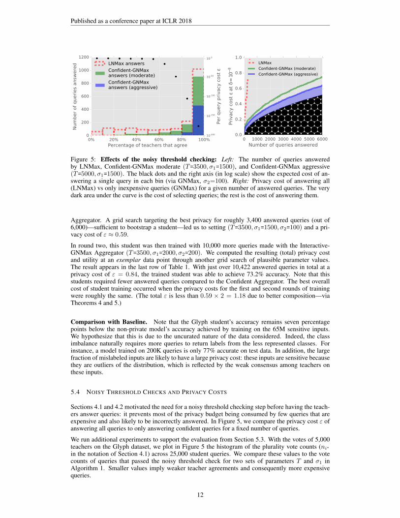
Aggregator. A grid search targeting the best privacy for roughly 3,400 answered queries (out of6,000)—sufficient to bootstrap a student—led us to setting (T=3500, σ1=1500, σ2=100) and a pri-vacy cost of ε ≈ 0.59.

In round two, this student was then trained with 10,000 more queries made with the Interactive-GNMax Aggregator (T=3500, σ1=2000, σ2=200). We computed the resulting (total) privacy costand utility at an exemplar data point through another grid search of plausible parameter values.The result appears in the last row of Table 1. With just over 10,422 answered queries in total at aprivacy cost of ε = 0.84, the trained student was able to achieve 73.2% accuracy. Note that thisstudents required fewer answered queries compared to the Confident Aggregator. The best overallcost of student training occurred when the privacy costs for the first and second rounds of trainingwere roughly the same. (The total ε is less than 0.59 × 2 = 1.18 due to better composition—viaTheorems 4 and 5.)

Comparison with Baseline. Note that the Glyph student’s accuracy remains seven percentagepoints below the non-private model’s accuracy achieved by training on the 65M sensitive inputs.We hypothesize that this is due to the uncurated nature of the data considered. Indeed, the classimbalance naturally requires more queries to return labels from the less represented classes. Forinstance, a model trained on 200K queries is only 77% accurate on test data. In addition, the largefraction of mislabeled inputs are likely to have a large privacy cost: these inputs are sensitive becausethey are outliers of the distribution, which is reflected by the weak consensus among teachers onthese inputs.

5.4 NOISY THRESHOLD CHECKS AND PRIVACY COSTS

Sections 4.1 and 4.2 motivated the need for a noisy threshold checking step before having the teach-ers answer queries: it prevents most of the privacy budget being consumed by few queries that areexpensive and also likely to be incorrectly answered. In Figure 5, we compare the privacy cost ε ofanswering all queries to only answering confident queries for a fixed number of queries.

We run additional experiments to support the evaluation from Section 5.3. With the votes of 5,000teachers on the Glyph dataset, we plot in Figure 5 the histogram of the plurality vote counts (ni∗in the notation of Section 4.1) across 25,000 student queries. We compare these values to the votecounts of queries that passed the noisy threshold check for two sets of parameters T and σ1 inAlgorithm 1. Smaller values imply weaker teacher agreements and consequently more expensivequeries.

12


When (T=3500, σ1=1500) we capture a significant fraction of queries where teachers have a strongconsensus (roughly > 4000 votes) while managing to filter out many queries with poor consensus.This moderate check ensures that although many queries with plurality votes between 2,500 and3,500 are answered (i.e., only 50–70% of teachers agree on a label) the expensive ones are mostlikely discarded. For (T=5000, σ1=1500), queries with poor consensus are completely culled out.This selectivity comes at the expense of a noticeable drop for queries that might have had a strongconsensus and little-to-no privacy cost. Thus, this aggressive check answer fewer queries with verystrong privacy guarantees. We reiterate that this threshold checking step itself is done in a privatemanner. Empirically, in our Interactive Aggregator experiments, we expend about a third to a half ofour privacy budget on this step, which still yields a very small cost per query across 6,000 queries.

6 CONCLUSIONS

The key insight motivating the addition of a noisy thresholding step to the two aggregation mecha-nisms proposed in our work is that there is a form of synergy between the privacy and accuracy oflabels output by the aggregation: labels that come at a small privacy cost also happen to be morelikely to be correct. As a consequence, we are able to provide more quality supervision to the studentby choosing not to output labels when the consensus among teachers is too low to provide an aggre-gated prediction at a small cost in privacy. This observation was further confirmed in some of ourexperiments where we observed that if we trained the student on either private or non-private labels,the former almost always gave better performance than the latter—for a fixed number of labels.

Complementary with these aggregation mechanisms is the use of a Gaussian (rather than Laplace)distribution to perturb teacher votes. In our experiments with Glyph data, these changes provedessential to preserve the accuracy of the aggregated labels—because of the large number of classes.The analysis presented in Section 4 details the delicate but necessary adaptation of analogous resultsfor the Laplace NoisyMax.

As was the case for the original PATE proposal, semi-supervised learning was instrumental to ensurethe student achieves strong utility given a limited set of labels from the aggregation mechanism.However, we found that virtual adversarial training outperforms the approach from Salimans et al.(2016) in our experiments with Glyph data. These results establish lower bounds on the performancethat a student can achieve when supervised with our aggregation mechanisms; future work maycontinue to investigate virtual adversarial training, semi-supervised generative adversarial networksand other techniques for learning the student in these particular settings with restricted supervision.

ACKNOWLEDGMENTS

We are grateful to Martín Abadi, Vincent Vanhoucke, and Daniel Levy for their useful inputs anddiscussions towards this paper.

13


REFERENCES

Martín Abadi, Andy Chu, Ian Goodfellow, H Brendan McMahan, Ilya Mironov, Kunal Talwar, andLi Zhang. Deep learning with differential privacy. In Proceedings of the 2016 ACM SIGSACConference on Computer and Communications Security, pp. 308–318. ACM, 2016.

Martín Abadi, Úlfar Erlingsson, Ian Goodfellow, H. Brendan McMahan, Nicolas Papernot, IlyaMironov, Kunal Talwar, and Li Zhang. On the protection of private information in machinelearning systems: Two recent approaches. In 2017 IEEE 30th Computer Security FoundationsSymposium (CSF), pp. 1–6, 2017.

Charu C Aggarwal. On k-anonymity and the curse of dimensionality. In Proceedings of the 31stInternational Conference on Very large Data Bases, pp. 901–909. VLDB Endowment, 2005.

Mitali Bafna and Jonathan Ullman. The price of selection in differential privacy. In Proceedings ofthe 2017 Conference on Learning Theory (COLT), volume 65 of Proceedings of Machine Learn-ing Research, pp. 151–168, July 2017.

Raef Bassily, Adam Smith, and Abhradeep Thakurta. Private empirical risk minimization: Efficientalgorithms and tight error bounds. In Proceedings of the 2014 IEEE 55th Annual Symposium onFoundations of Computer Science (FOCS), pp. 464–473, 2014. ISBN 978-1-4799-6517-5.

Raghav Bhaskar, Srivatsan Laxman, Adam Smith, and Abhradeep Thakurta. Discovering frequentpatterns in sensitive data. In Proceedings of the 16th ACM SIGKDD international conference onKnowledge discovery and data mining, pp. 503–512. ACM, 2010.

Battista Biggio, Igino Corona, Davide Maiorca, Blaine Nelson, Nedim Šrndic, Pavel Laskov, Gior-gio Giacinto, and Fabio Roli. Evasion attacks against machine learning at test time. In JointEuropean Conference on Machine Learning and Knowledge Discovery in Databases, pp. 387–402, 2013.

Vincent Bindschaedler, Reza Shokri, and Carl A Gunter. Plausible deniability for privacy-preservingdata synthesis. Proceedings of the VLDB Endowment, 10(5), 2017.

Mark Bun and Thomas Steinke. Concentrated differential privacy: Simplifications, extensions, andlower bounds. In Theory of Cryptography Conference (TCC), pp. 635–658, 2016.

Mark Bun, Thomas Steinke, and Jonathan Ullman. Make up your mind: The price of online queriesin differential privacy. In Proceedings of the Twenty-Eighth Annual ACM-SIAM Symposium onDiscrete Algorithms, pp. 1306–1325. SIAM, 2017.

Kamalika Chaudhuri, Claire Monteleoni, and Anand D Sarwate. Differentially private empiricalrisk minimization. Journal of Machine Learning Research, 12(Mar):1069–1109, 2011.

David Cohn, Les Atlas, and Richard Ladner. Improving generalization with active learning. Machinelearning, 15(2):201–221, 1994.

Cynthia Dwork and Aaron Roth. The algorithmic foundations of differential privacy. Foundationsand Trends in Theoretical Computer Science, 9(3–4):211–407, 2014.

Cynthia Dwork and Guy N Rothblum. Concentrated differential privacy. arXiv preprintarXiv:1603.01887, 2016.

Cynthia Dwork, Frank McSherry, Kobbi Nissim, and Adam Smith. Calibrating noise to sensitivity inprivate data analysis. In Proceedings of the Third Conference on Theory of Cryptography (TCC),volume 3876, pp. 265–284, 2006.

Cynthia Dwork, Guy N Rothblum, and Salil Vadhan. Boosting and differential privacy. In Pro-ceedings of the 51st Annual IEEE Symposium on Foundations of Computer Science (FOCS), pp.51–60, 2010.

Jihun Hamm, Yingjun Cao, and Mikhail Belkin. Learning privately from multiparty data. In Inter-national Conference on Machine Learning (ICML), pp. 555–563, 2016.

14

http://arxiv.org/abs/1603.01887


Steve Hanneke. Theory of disagreement-based active learning. Foundations and Trends in MachineLearning, 7(2-3):131–309, 2014.

Moritz Hardt and Guy N Rothblum. A multiplicative weights mechanism for privacy-preservingdata analysis. In 51st Annual IEEE Symposium on Foundations of Computer Science (FOCS), pp.61–70, 2010.

Kaiming He, Xiangyu Zhang, Shaoqing Ren, and Jian Sun. Deep residual learning for image recog-nition. In 2016 IEEE Conference on Computer Vision and Pattern Recognition (CVPR), pp.770–778, 2016.

Ron Kohavi. Scaling up the accuracy of Naive-Bayes classifiers: A decision-tree hybrid. In KDD,volume 96, pp. 202–207, 1996.

Yun Liu, Krishna Gadepalli, Mohammad Norouzi, George E Dahl, Timo Kohlberger, AlekseyBoyko, Subhashini Venugopalan, Aleksei Timofeev, Philip Q Nelson, Greg S Corrado, et al.Detecting cancer metastases on gigapixel pathology images. arXiv preprint arXiv:1703.02442,2017.

H Brendan McMahan, Daniel Ramage, Kunal Talwar, and Li Zhang. Learning differentially privatelanguage models without losing accuracy. arXiv preprint arXiv:1710.06963, 2017.

Frank McSherry and Kunal Talwar. Mechanism design via differential privacy. In Proceedings of the48th Annual IEEE Symposium on Foundations of Computer Science (FOCS), pp. 94–103, 2007.

Ilya Mironov. Rényi differential privacy. In 2017 IEEE 30th Computer Security Foundations Sym-posium (CSF), pp. 263–275, 2017.

Takeru Miyato, Shin-ichi Maeda, Masanori Koyama, and Shin Ishii. Virtual adversarial train-ing: a regularization method for supervised and semi-supervised learning. arXiv preprintarXiv:1704.03976, 2017.

Arvind Narayanan and Vitaly Shmatikov. Robust de-anonymization of large sparse datasets. InProceedings of the 2008 IEEE Symposium on Security and Privacy, pp. 111–125. IEEE, 2008.

Yuval Netzer, Tao Wang, Adam Coates, Alessandro Bissacco, Bo Wu, and Andrew Y Ng. Readingdigits in natural images with unsupervised feature learning. In NIPS Workshop on Deep Learningand Unsupervised Feature Learning, pp. 5, 2011.

Kobbi Nissim, Sofya Raskhodnikova, and Adam Smith. Smooth sensitivity and sampling in pri-vate data analysis. In Proceedings of the Thirty-ninth Annual ACM Symposium on Theory ofComputing (STOC), pp. 75–84, 2007.

Nicolas Papernot, Martín Abadi, Úlfar Erlingsson, Ian Goodfellow, and Kunal Talwar. Semi-supervised knowledge transfer for deep learning from private training data. In Proceedings ofthe 5th International Conference on Learning Representations (ICLR), 2017.

Manas Pathak, Shantanu Rane, and Bhiksha Raj. Multiparty differential privacy via aggregation oflocally trained classifiers. In Advances in Neural Information Processing Systems, pp. 1876–1884,2010.

Aaron Roth and Tim Roughgarden. Interactive privacy via the median mechanism. In Proceedingsof the Forty-second ACM Symposium on Theory of Computing (STOC), pp. 765–774, 2010.

Tim Salimans, Ian Goodfellow, Wojciech Zaremba, Vicki Cheung, Alec Radford, and Xi Chen.Improved techniques for training GANs. In Advances in Neural Information Processing Systems,pp. 2234–2242, 2016.

Reza Shokri, Marco Stronati, Congzheng Song, and Vitaly Shmatikov. Membership inference at-tacks against machine learning models. In Proceedings of the 2017 IEEE Symposium on Securityand Privacy, pp. 3–18. IEEE, 2017.

Shuang Song, Kamalika Chaudhuri, and Anand D Sarwate. Stochastic gradient descent with differ-entially private updates. In 2013 IEEE Global Conference on Signal and Information Processing,pp. 245–248, 2013.

15





Thomas Steinke and Jonathan Ullman. Tight lower bounds for differentially private selection. In58th IEEE Annual Symposium on Foundations of Computer Science (FOCS), pp. 552–563, 2017.

Christian Szegedy, Wojciech Zaremba, Ilya Sutskever, Joan Bruna, Dumitru Erhan, Ian Goodfellow,and Rob Fergus. Intriguing properties of neural networks. In Proceedings of the 2nd InternationalConference on Learning Representations (ICLR), 2014.

Florian Tramèr, Fan Zhang, Ari Juels, Michael K Reiter, and Thomas Ristenpart. Stealing machinelearning models via prediction APIs. In USENIX Security Symposium, pp. 601–618, 2016.

Tim van Erven and Peter Harremoës. Rényi divergence and Kullback-Leibler divergence. IEEETransactions on Information Theory, 60(7):3797–3820, July 2014.

Chiyuan Zhang, Samy Bengio, Moritz Hardt, Benjamin Recht, and Oriol Vinyals. Understandingdeep learning requires rethinking generalization. In Proceedings of the 5th International Confer-ence on Learning Representations (ICLR), 2017.

16


A APPENDIX: PRIVACY ANALYSIS

In this appendix, we provide the proofs of Theorem 6 and Proposition 7. Moreover, we presentProposition 10, which provides optimal values of µ1 and µ2 to apply towards Theorem 6 for theGNMax mechanism. We start off with a statement about the Rényi differential privacy guarantee ofthe GNMax.

Proposition 8. The GNMax aggregatorMσ guarantees(λ, λ/σ2

)-RDP for all λ ≥ 1.

Proof. The result follows from observing thatMσ can be decomposed into applying the argmaxoperator to a noisy histogram resulted from adding Gaussian noise to each dimension of the originalhistogram. The Gaussian mechanism satisfies (λ, λ/2σ2)-RDP (Mironov, 2017), and since eachteacher may change two counts (incrementing one and decrementing the other), the overall RDPguarantee is as claimed.

Proposition 7. For a GNMax aggregator Mσ , the teachers’ votes histogram n = (n1, . . . , nm),and for any i∗ ∈ [m], we have

Pr [Mσ(D) 6= i∗] ≤ q(n),

where

q(n) ,1

2

∑i 6=i∗

erfc

(ni∗ − ni

2σ

).

Proof. Recall thatMσ(D) = argmax(ni + Zi), where Zi are distributed as N (0, σ2). Then forany i∗ ∈ [m], we have

Pr[Mσ(D) 6= i∗] = Pr [∃i, ni + Zi > ni∗ + Zi∗ ] ≤∑i 6=i∗

Pr [ni + Zi > ni∗ + Zi∗ ]

=∑i 6=i∗

Pr [Zi − Zi∗ > ni∗ − ni]

=∑i 6=i∗

1

2

(1− erf

(ni∗ − ni

2σ

)).

where the last equality follows from the fact that Zi − Zj is a Gaussian random variable with meanzero and variance 2σ2.

We now present a precise statement of Theorem 6.

Theorem 6. LetM be a randomized algorithm with (µ1, ε1)-RDP and (µ2, ε2)-RDP guaranteesand suppose that there exists a likely outcome i∗ given a dataset D and a bound q ≤ 1 such that

q ≥ Pr [M(D) 6= i∗]. Additionally suppose that λ ≤ µ1 and q ≤ e(µ2−1)ε2/(

µ1

µ1−1 ·µ2

µ2−1

)µ2

.

Then, for any neighboring dataset D′ of D, we have:

Dλ(M(D)‖M(D′)) ≤ 1

λ− 1log(

(1− q) ·A(q, µ2, ε2)λ−1 + q ·B(q, µ1, ε1)λ−1)

(2)

whereA(q, µ2, ε2) , (1− q)/(

1− (qeε2)µ2−1µ2

)andB(q, µ1, ε1) , eε1/q

1µ1−1 .

Proof. Before we proceed to the proof, we introduce some simplifying notation. For a randomizedmechanismM and neighboring datasets D and D′, we define

βM(λ;D,D′) , Dλ(M(D)‖M(D′))

=1

λ− 1logEx∼M(D)

[(Pr [M(D) = x]

Pr [M(D′) = x]

)λ−1].

As the proof involves working with the RDP bounds in the exponent, we set ζ1 , eε1(µ1−1) andζ2 , eε2(µ2−1).

17


Finally, we define the following shortcuts:

qi , Pr [M(D) = i] and q ,∑i 6=i∗

qi = Pr [M(D) 6= i∗] ,

pi , Pr [M(D′) = i] and p ,∑i6=i∗

pi = Pr [M(D′) 6= i∗] ,

and note that q ≤ q.

From the definition of Rényi differential privacy, (µ1, ε1)-RDP implies:

exp (βM(µ1;D,D′)) =

(1− q)µ1

(1− p)µ1−1+∑i6=i∗

qµ1

i

pµ1−1i

1/(µ1−1)

≤ exp(ε1)

=⇒∑i>1

qµ1

i

pµ1−1i

=∑i>1

qi

(qipi

)µ1−1

≤ ζ1. (3)

Since µ1 ≥ λ, f(x) , xµ1−1λ−1 is convex. Applying Jensen’s Inequality we have the following:

∑i 6=i∗ qi

(qipi

)λ−1

q

µ1−1λ−1

≤

∑i 6=i∗ qi

(qipi

)µ1−1

q

=⇒∑i6=i∗

qi

(qipi

)λ−1

≤ q

∑i 6=i∗ qi

(qipi

)µ1−1

q

λ−1µ1−1

(3)=⇒

∑i6=i∗

qi

(qipi

)λ−1

≤ ζ1λ−1µ1−1 · q1− λ−1

µ1−1 . (4)

Next, by the bound at order µ2, we have:

exp (βM(µ2;D′, D)) =

(1− p)µ2

(1− q)µ2−1+∑i 6=i∗

pµ2

i

qµ2−1i

1/(µ2−1)

≤ exp(ε2)

=⇒ (1− p)µ2

(1− q)µ2−1+∑i6=i∗

pµ2

i

qµ2−1i

≤ ζ2.

By the data processing inequality of Rényi divergence, we have

(1− p)µ2

(1− q)µ2−1+

pµ2

qµ2−1≤ ζ2,

which implies pµ2

qµ2−1 ≤ ζ2 and thus

p ≤(qµ2−1ζ2

) 1µ2 . (5)

Combining (4) and (5), we can derive a bound at λ.

exp (βM(λ,D,D′)) =

(1− q)λ

(1− p)λ−1+∑i6=i∗

qλipλ−1i

1/(λ−1)

≤

(1− q)λ(1− (qµ2−1ζ2)

1µ2

)λ−1+ ζ1

λ−1µ1−1 · q1− λ−1

µ1−1

1/(λ−1)

. (6)

18


Although Equation (6) is very close to the corresponding statement in the theorem’s claim, onesubtlety remains. The bound (6) applies to the exact probability q = Pr [M(D) 6= i∗]. In thetheorem statement, and in practice, we can only derive an upper bound q on Pr [M(D) 6= i∗]. Thelast step of the proof requires showing that the expression in Equation (6) is monotone in the rangeof values of q that we care about.

Lemma 9 (Monotonicity of the bound). Let the functions f1(·) and f2(·) be

f1(x) ,(1− x)λ(

1− (xµ2−1ζ2)1µ2

)λ−1and f2(x) , ζ1

λ−1µ1−1 · x1− λ−1

µ1−1 ,

Then f1(x) + f2(x) is increasing in[0,min

(1, ζ2/

(µ1

µ1−1 ·µ2

µ2−1

)µ2)]

.

Proof. Taking the derivative of f1(x), we have:

f ′1(x) =−λ(1− x)λ−1(1− (xµ2−1ζ2)

1µ2 )λ−1

(1− (xµ2−1ζ2)1µ2 )2λ−2

+(1− x)λ(λ− 1)(1− (xµ2−1ζ2)

1µ2 )λ−2ζ2

1µ2 · µ2−1

µ2· x−

1µ2

(1− (xµ2−1ζ2)1µ2 )2λ−2

=(1− x)λ−1

(1− (xµ2−1ζ2)1µ2 )λ−1

(−λ+ (λ− 1)

(1− 1

µ2

)1− x

1− (xµ2−1ζ2)1µ2

(ζ2x

) 1µ2

).

We intend to show that:

f ′1(x) ≥ −λ+ (λ− 1)

(1− 1

µ2

)(ζ2x

) 1µ2

. (7)

For x ∈[0, ζ2/

(µ1

µ1−1 ·µ2

µ2−1

)µ2]

and y ∈ [1,∞), define g(x, y) as:

g(x, y) , −λ · yλ−1 + (λ− 1)

(1− 1

µ2

)(ζ2x

) 1µ2

yλ.

We claim that g(x, y) is increasing in y and therefore g(x, y) ≥ g(x, 1), and prove it by showing thepartial derivative of g(x, y) with respect to y is non-negative. Take a derivative with respect to y as:

g′y(x, y) = −λ(λ− 1)yλ−2 + λ(λ− 1)

(1− 1

µ2

)(ζ2x

) 1µ2

yλ−1

= λ(λ− 1)yλ−2

(−1 +

(1− 1

µ2

)(ζ2x

) 1µ2

y

).

To see why g′y(x, y) is non-negative in the respective ranges of x and y, note that:

x ≤ ζ2/(

µ1

µ1 − 1· µ2

µ2 − 1

)µ2

=⇒ x ≤ ζ2/(

µ2

µ2 − 1

)µ2

=⇒ 1 ≤ ζ2x·(µ2 − 1

µ2

)µ2

=⇒ 1 ≤ µ2 − 1

µ2

(ζ2x

) 1µ2

=⇒ 1 ≤ µ2 − 1

µ2

(ζ2x

) 1µ2

y (as y ≥ 1)

=⇒ 0 ≤ −1 +µ2 − 1

µ2

(ζ2x

) 1µ2

y

=⇒ 0 ≤ g′y(x, y). (in the resp. range of x and y)

19


Consider 1−x1−(xµ2−1ζ2)1/µ2

. Since ζ2 ≥ 1 and x ≤ 1, we have x ≤ ζ2 and hence

1− x1− (xµ2−1ζ2)

1µ2

≥ 1− x1− (xµ2−1x)

1µ2

= 1.

Therefore we can set y = 1−x1−(xµ2−1ζ2)1/µ2

and apply the fact that g(x, y) ≥ g(x, 1) for all y ≥ 1 toget

f ′1(x) ≥ −λ+ (λ− 1)

(1− 1

µ2

)(ζ2x

) 1µ2

,

as required by (7).

Taking the derivative of f2(x), we have:

f ′2(x) = ζ1λ−1µ1−1 ·

(1− λ− 1

µ1 − 1

)x−

λ−1µ1−1 =

(ζ1x

) λ−1µ1−1

(1− λ− 1

µ1 − 1

)≥ 1− λ− 1

µ1 − 1.

Combining the two terms together, we have:

f ′(x) ≥ −λ+ (λ− 1)

(1− 1

µ2

)(ζ2x

) 1µ2

+ 1− λ− 1

µ1 − 1

= (λ− 1)

(− µ1

µ1 − 1+µ2 − 1

µ2

(ζ2x

) 1µ2

).

For f ′(x) to be non-negative we need:

− µ1

µ1 − 1+µ2 − 1

µ2

(ζ2x

) 1µ2

≥ 0

⇐⇒(

µ1

µ1 − 1· µ2

µ2 − 1

)µ2

≤ ζ2x.

So f(x) is increasing for x ∈[0, ζ2/

(µ1

µ1−1 ·µ2

µ2−1

)µ2]. This means for q ≤ q ≤

ζ2/(

µ1

µ1−1 ·µ2

µ2−1

)µ2

, we have f(q) ≤ f(q). This completes the proof of the lemma and that of

the theorem.

Theorem 6 yields data-dependent Rényi differential privacy bounds for any value of µ1 and µ2 largerthan λ. The following proposition simplifies this search by calculating optimal higher moments µ1

and µ2 for the GNMax mechanism with variance σ2.Proposition 10. When applying Theorem 6 and Proposition 8 for GNMax with Gaussian of varianceσ2, the right-hand side of (2) is minimized at

µ2 = σ ·√

log(1/q), and µ1 = µ2 + 1.

Proof. We can minimize both terms in (2) independently. To minimize the first term in (6), weminimize (qeε2)

1−1/µ2 by considering logarithms:

log{

(qeε2)1−1/µ2

}= log

{q1− 1

µ2 exp

(µ2 − 1

σ2

)}=

(1− 1

µ2

)· log q +

µ2 − 1

σ2

=1

µ2log

1

q+µ2

σ2− 1

σ2− log

1

q,

20


which is minimized at µ2 = σ ·√

log(1/q).

To minimize the second term in (6), we minimize eε1/q1/(µ1−1) as follows:

log

{eε1

q1/(µ1−1)

}= log

{q−1/(µ1−1) exp

(µ1

σ2

)}=µ1

σ2+

1

µ1 − 1log

1

q

=1

σ2+µ1 − 1

σ2+

1

µ1 − 1log

1

q,

which is minimized at µ1 = 1 + σ ·√

log(1/q) completing the proof.

Putting this together, we apply the following steps to calculate RDP of order λ for GNMax withvariance σ2 on a given dataset D. First, we compute a bound q according to Proposition 7. Then weuse the smaller of two bounds: a data-dependent (Theorem 6) and a data-independent one (Proposi-tion 8) :

βσ(q) , min

{1

λ− 1log{

(1− q) ·A(q, µ2, ε2)λ−1 + q ·B(q, µ1, ε1)λ−1}, λ/σ2

},

whereA andB are defined as in the statement of Theorem 6, the parameters µ1 and µ2 are selectedaccording to Proposition 10, and ε1 , µ1/σ

2 and ε2 , µ2/σ2 (Proposition 8). Importantly, the first

expression is evaluated only when q < 1, µ1 ≥ λ, µ2 > 1, and q ≤ e(µ2−1)ε2/(

µ1

µ1−1 ·µ2

µ2−1

)µ2

.These conditions can either be checked for each application of the aggregation mechanism, or a crit-ical value of q0 that separates the range of applicability of the data-dependent and data-independentbounds can be computed for given σ and λ. In our implementation we pursue the second approach.

The following corollary offers a simple asymptotic expression of the privacy of GNMax for the casewhen there are large (relative to σ) gaps between the highest three vote counts.

Corollary 11. If the top three vote counts are n1 > n2 > n3 and n1 − n2, n2 − n3 � σ,then the mechanism GNMax with Gaussian of variance σ2 satisfies (λ, exp(−2λ/σ2)/λ)-RDP forλ = (n1 − n2)/4.

Proof. Denote the noisy counts as ni = ni + N (0, σ2). Ignoring outputs other than those withthe highest and the second highest counts, we bound q = Pr [M(D) 6= 1] as Pr[n1 < n2] =Pr[N(0, 2σ2) > n1 − n2] < exp

(−(n1 − n2)2/4σ2

), which we use as q. Plugging q in Proposi-

tion 10, we have µ1 − 1 = µ2 = (n1 − n2)/2, limiting the range of applicability of Theorem 6 toλ < (n1 − n2)/2.

Choosing λ = (n1−n2)/4 ensuresA(q, µ2, ε2) ≈ 1, which allows approximating the bound (2) asq ·B(q, µ1, ε1)λ−1/(λ− 1). The proof follows by straightforward calculation.

B SMOOTH SENSITIVITY AND PUBLISHING THE PRIVACY PARAMETER

The privacy guarantees obtained for the mechanisms in this paper via Theorem 6 take as input q, anupper bound on the probability that the aggregate mechanism returns the true plurality. This meansthat the resulting privacy parameters computed depend on teacher votes and hence the underlyingdata. To avoid potential privacy breaches from simply publishing the data-dependent parameter, weneed to publish a sanitized version of the privacy loss. This is done by adding noise to the computedprivacy loss estimates using the smooth sensitivity algorithm proposed by Nissim et al. (2007).

This section has the following structure. First we recall the notion of smooth sensitivity and intro-duce an algorithm for computing the smooth sensitivity of the privacy loss function of the GNMaxmechanism. In the rest of the section we prove correctness of these algorithms by stating severalconditions on the mechanism, proving that these conditions are sufficient for correctness of the al-gorithm, and finally demonstrating that GNMax satisfies these conditions.

21


B.1 COMPUTING SMOOTH SENSITIVITY

Any dataset D defines a histogram n = (n1, . . . , nm) ∈ Nm of the teachers’ votes. We have anatural notion of the distance between two histograms dist(n, n′) and a function q:Nm → [0, 1]on these histograms computing the bound according to Proposition 7. The value q(n) can be usedas q in the application of Theorem 6. Additionally we have n(i) denote the i-th highest bar in thehistogram.

We aim at calculating a smooth sensitivity of β (q(n)) whose definition we recall now.Definition 12 (Smooth Sensitivity). Given the smoothness parameter β, a β-smooth sensitivity off(n) is defined as

SSβ(n) , maxd≥0

e−βd · maxn′:dist(n,n′)≤d

LS(n′),

where

LS(n) ≥ maxn′:dist(n,n′)=1

|f(n)− f(n′)|

is an upper bound on the local sensitivity.

We now describe Algorithms 3–5 computing a smooth sensitivity of β (q(·)). The algorithms as-sume the existence of efficiently computable functions q:Nm → [0, 1], BL,BU: [0, 1] → [0, 1], anda constant q0.

Informally, the functions BU and BL respectively upper and lower bound the value of q evaluated atany neighbor of n given q(n), and [0, q0) limits the range of applicability of data-dependent analysis.

The functions BL and BU are defined as follows. Their derivation appears in Section B.4.

BU(q) , min

{m− 1

2erfc

(erfc-1

(2q

m− 1

)− 1

σ

), 1

},

BL(q) ,m− 1

2erfc

(erfc-1

(2q

m− 1

)+

1

σ

),

Algorithm 3 – Local Sensitivity: use the functions BU and BL to compute (an upper bound) of thelocal sensitivity at a given q value by looking at the difference of β (·) evaluated on the bounds.

1: procedure LS(q)2: if q1 ≤ q ≤ q0 then . q1 = BL(q0). Interpolate the middle part.3: q ← q1

4: end if5: return max{β (BU(q))− β (q) ,β (q)− β (BL(q))}6: end procedure

B.2 NOTATION AND CONDITIONS

Notation. We find that the algorithm and the proof of its correctness are more naturally expressedif we relax the notions of a histogram and its neighbors to allow non-integer values.

• We generalize histograms to be any vector with non-negative real values. This relaxation isused only in the analysis of algorithms; the actual computations are performed exclusivelyover integer-valued inputs.

• Let n = [n1, . . . , nm] ∈ Rm, ni ≥ 0 denote a histogram. Let n(i) denote the i-th bar in thedescending order.

• Define a “move” as increasing one bar by some value in [0, 1] and decreasing one bar by a(possibly different) value in [0, 1] subject to the resulting value be non-negative. Notice thedifference between the original problem and our relaxation. In the original formulation, thehistogram takes only integer values and we can only increase/decrease them by exactly 1.In contrast, we allow real values and a teacher can contribute an arbitrary amount in [0, 1]to any one class.

22


Algorithm 4 – Sensitivity at a distance: given a histogram n, compute the sensitivity of β (·) atdistance at most d using the procedure LS, function q(·), constants q0 and q1 = BL(q0), and carefulcase analysis that finds the neighbor at distance d with the maximum sensitivity.

1: procedure ATDISTANCED(n, d)2: q ← q(n)3: if q1 ≤ q ≤ q0 then . q is in the flat region.4: return LS(q), STOP5: end if6: if q < q1 then . Need to increase q.7: if n(1) − n(2) < 2d then . n(i) is the ith largest element.8: return LS(q1), STOP9: else

10: n′ ← SORT(n) + [−d, d, 0, . . . , 0]11: q′ ← q(n′)12: if q′ > q1 then13: return LS(q0), STOP14: else15: return LS(q′), CONTINUE16: end if17: end if18: else . Need to decrease q.19: if

∑di=2 n

(i) ≤ d then20: n′ ← [n, 0, . . . , 0]21: q′ ← q(n′)

22: return LS(q′), STOP23: else24: n′ ← SORT(n) + [d, 0, . . . , 0]25: for d′ = 1, . . . , d do26: n′(2) ← n′(2) − 1 . The index of n′(2) may change.27: end for28: q′ ← q(n′)29: if q′ < q0 then30: return LS(q0), STOP31: else32: return LS(q′), CONTINUE33: end if34: end if35: end if36: end procedure

Algorithm 5 – Smooth Sensitivity: Compute the β smooth sensitivity of β (·) via Definition 12 bylooking at sensitivities at various distances and returning the maximum weighted by e−βd.

1: procedure SMOOTHSENSITIVITY(n, β)2: S ← 03: d← 04: repeat5: c,StoppingCondition← ATDISTANCED(n, d)6: S ← max{S, c · e−βd}7: d← d+ 18: until StoppingCondition = STOP9: end procedure

• Define the distance between two histograms n = (n1, . . . , nm) and n′ = (n′1, . . . , n′m) as

d(n, n′) , max

∑i:ni>n′i

dni − n′ie,∑

i:ni<n′i

dn′i − nie

,

23


which is equal to the smallest number of “moves” needed to make the two histogramsidentical. We use the ceiling function since a single step can increase/decrease one bar byat most 1.We say that two histograms are neighbors if their distance d is 1.Notice that analyses of Rényi differential privacy for LNMax, GNMax and the exponentialmechanism are still applicable when the neighboring datasets are defined in this manner.

• Given a randomized aggregatorM:Rm≥0 → [m], let q:Rm≥0 → [0, 1] be so that

q(n) ≥ Pr[M(n) 6= argmax(n)].

When the context is clear, we use q to denote a specific value of the function, which, inparticular, can be used as q in applications of Theorem 6.

• Let β: [0, 1]→ R be the function that maps a q value to the value of the Rényi accountant.

Conditions. Throughout this section we will be referring to the list of conditions on q(·) and β (·):

C1. The function q(·) is continuous in each argument ni.C2. There exist functions BU,BL: [0, 1] → [0, 1] such that for any neighbor n′ of n, we have

BL(q(n)) ≤ q(n′) ≤ BU(q(n)), i.e., BU and BL provide upper and lower bounds on theq value of any neighbor of n.

C3. BL(q) is increasing in q.C4. BU and BL are functional inverses of each other in part of the range, i.e., q = BL(BU(q))

for all q ∈ [0, q0], where q0 is defined below. Additionally BL(q) ≤ q ≤ BU(q) for allq ∈ [0, 1].

C5. β (·) has the following shape: there exist constants β∗ and q0 ≤ 0.5, such that β (q) non-decreasing in [0, q0] and β (q) = β∗ ≥ β (q0) for q > q0. The constant β∗ corresponds toa data-independent bound.

C6. ∆β (q) , β (BU(q))− β (q) is non-decreasing in [0,BL(q0)], i.e., when BU(q) ≤ q0.

C7. Recall that n(i) is the i-th largest coordinate of a histogram n. Then, if q(n) ≤ BU(q0),then q(n) is differentiable in all coordinates and

∀i > j ≥ 2∂q

∂n(j)(n) ≥ ∂q

∂n(i)(n) ≥ 0.

C8. The function q(n) is invariant under addition of a constant, i.e.,

q(n) = q(n+ [x, . . . , x]) for all n and x ≥ 0,

and q(n) is invariant under permutation of n, i.e.,

q(n) = q(π(n)) for all permutations π on [m].

Finally, we require that if n(1) = n(2), then q(n) ≥ q0.

We may additionally assume that q0 ≥ q([n, 0, . . . , 0]). Indeed, if this condition is not satisfied,then the data-dependent analysis is not going to be used anywhere. The most extreme histogram—[n, 0, . . . , 0]—is the most advantageous setting for applying data-dependent bounds. If we cannotuse the data-dependent bound even in that case, we would be using the data-independent boundeverywhere and do not need to compute smooth sensitivity anyway. Yet this condition is not auto-matically satisfied. For example, if m (the number of classes) is large compared to n (the numberof teachers), we might have large q([n, 0, . . . , 0]). So we need to check this condition in the codebefore doing smooth sensitivity calculation.

B.3 CORRECTNESS OF ALGORITHMS 3–5

Recall that local sensitivity of a deterministic function f is defined as max f(D)− f(D′), where Dand D′ are neighbors.Proposition 13. Under conditions C2–C6, Algorithm 3 computes an upper bound on local sensitiv-ity of β (q(n)).

24


Proof. Since β (·) is non-decreasing everywhere (by C5), and for any neighbors n and n′ it holdsthat BL(q(n)) ≤ q(n′) ≤ BU(q(n)) (by C2), we have the following

|β (q(n))− β (q(n′))| ≤ max

{β(

BU(q(n)))− β

(q(n)

), β(q(n)

)− β

(BL(q(n))

)}= max

{∆β(q(n)

), ∆β

(BL(q(n))

)}as an upper bound on the local sensitivity of β (q(·)) at input n.

The function computed by Algorithm 3 differs from above when q(n) ∈ (BL(q0), q0). To completethe proof we need to argue that the local sensitivity is upper bounded by ∆β (BL(q0)) for q(n) inthis interval. The bound follows from the following three observations.

First, ∆β (q) is non-increasing in the range (BL(q0), 1], since β (BU(q)) is constant (by BU(q) ≥BU(BL(q0)) = q0 and C5) and β (q) is non-decreasing in the range (by C5). In particular,

∆β (q) ≤ ∆β (BL(q0)) if q ≥ BL(q0). (8)Second, ∆β (BL(q)) is non-decreasing in the range [0, q0] since BL(q) is increasing (by C3 and C6).This implies that

∆β (BL(q)) ≤ ∆β (BL(q0)) if q ≤ q0. (9)

By (8) and (9) applied to the intersection of the two ranges, it holds that

max

{∆β(q(n)

), ∆β

(BL(q(n))

)}≤ ∆β (BL(q0)) if BL(q0) ≤ q ≤ q0,

as needed.

We thus established that the function computed by Algorithm 3, which we call LS(q) from now on,is an upper bound on the local sensitivity. Formally,

LS(q) ,

{∆β (BL(q0)) if q ∈ (BL(q0), q0),

max {∆β (q) ,∆β (BL(q))} otherwise.

The following proposition characterizes the growth of LS(q).

Proposition 14. Assuming conditions C2–C6, the function LS(q) is non-decreasing in [0,BL(q0)],constant in [BL(q0), q0], and non-increasing in [q0, 1].

Proof. Consider separately three intervals.

• By construction, LS is constant in [BL(q0), q0].

• Since both functions ∆β (·) and ∆β (BL(·)) are each non-decreasing in [0,BL(q0)), so istheir max.

• In the interval (q0, 1], β (q) is constant. Hence ∆β (q) = 0 and ∆β (BL(q)) = β (q) −β (BL(q)) is non-decreasing. Their maximum value ∆β (BL(q)) is non-decreasing.

The claim follows.

We next prove correctness of Algorithm 4, which computes the maximal sensitivity of β at a fixeddistance.

The proof relies on the following notion of a partial order between histograms.Definition 15. Prefix sums Si(n) are defined as follows:

Si(n) ,i∑

j=1

(n(1) − n(j)).

We say that a histogram n dominates n′, denoted as n � n′, iff:∀ (1 < i ≤ m) it holds that Si(n) ≥ Si(n′).

25


The function q(·) is monotone under this notion of dominance (assuming certain conditions hold):Proposition 16. If q(·) satisfies C1, C2, C7, and C8, and q(n) < BU(q0), then

n � n′ ⇒ q(n) ≤ q(n′).

Proof. We may assume that n(1) = n′(1). Indeed, if this does not hold, add |n(1) − n′(1)| to allcoordinates of the histogram with the smaller of the two values. This transform does not change theq value (by C8) and it preserves the � relationship as all prefix sums Si(·) remain unchanged.

We make a simple observation that will be helpful later:

∀i ∈ [m] it holds thati∑

j=1

(n(1) − nj) ≥ Si(n). (10)

The inequality holds because the prefix sum accumulates the gaps between the largest value of nand all other values in the non-decreasing order. Any deviation from this order may only increasethe prefix sums.

The following lemma constructs a monotone chain (in the partial order of dominance) of histogramsconnecting n and n′ via a sequence of intermediate steps that either do not change the value of q ortouch at most two coordinates at a time.

Lemma 17. There exists a chain n = n0 � n1 � · · · � nd = n′, such that for all i ∈ [d] eitherd(ni−1, ni) = 1 or ni−1 = π(ni) for some permutation π on [m]. Additionally, n(1)

0 = · · · = n(1)d .

Proof (Lemma). Wlog we assume that n and n′ are each sorted in the descending order. The proofis by induction on `(n, n′) ,

∑idni − n′ie ≤ 2d(n, n′), which, by construction, only assumes

non-negative integer values.

If the distance is 0, the statement is immediate. Otherwise, find the smallest i so that Si(n) > Si(n′)

(if all prefix sums are equal and n(1) = n′(1), it would imply that n = n′). In particular, it meansthat nj = n′j for j < i and ni < n′i ≤ ni−1 = n′i−1. Let x , min(n′i − ni, 1). Define n′′ asidentical to n′ except that n′′i = n′i − x. The new value is guaranteed to be non-negative, sincex ≤ n′i−ni and ni ≥ 0. Note that n′′ is not necessarily sorted anymore. Consider two possibilities.

Case I: n � n′′. Since n′′ � n′, `(n, n′′) < `(n, n′), and d(n′′, n′) = 1, we may apply theinduction hypothesis to the pair n, n′′.

Case II: n � n′′. This may happen because the prefix sums of n′′ increase compared to Sj(n′) forj ≥ i. Find the smallest such i′ so that

∑i′

j=1(n′′1 − n′′j ) > Si′(n). (Since n′′ is not sorted, we fixthe order in which prefix sums are accumulated to be the same as in n; by (10) i′ is well defined).Next we let n′′′ be identical to n′′ except that n′′′i′ = n′′i′ + x. In other words, n′′′ differs from n′ byshifting x from coordinate i to coordinate i′.

We argue that incrementing n′′i′ by x does not change the maximal value of n′′, i.e., n′′′1 > n′′′i′ . Ourchoice of i′, which is the smallest index so that the prefix sum over n′′ overtakes that over n, impliesthat n′′1 − n′′i′ > n1 − ni′ . Since n′′1 = n1, it means that ni′ > n′′i′ (and by adding x we move n′′i′towards ni′ ). Furthermore,

n′′′i′ = n′′i′ + x ≤ ni′ + (n′i − ni) = n′i + (ni′ − ni) ≤ n′i ≤ n′1 = n′′′1 ,

(We use ni′ ≤ ni, which is implied by i′ > i.)

We claim that∑tj=1(n′′′1 − n′′′j ) ≤ St(n) for all t, and thus, via (10), n � n′′′. The choice of i′

makes the statement trivial for t < i′. For t ≥ i′ the following holds:

t∑j=1

(n′′′1 − n′′′j ) =

t∑j=1

(n′′1 − n′′j )− x ≤

t∑j=1

(n′1 − n′j) + x

− x = St(n′) ≤ St(n).

By construction d(n′, n′′′) = 1 (the two histograms differ in two locations, in positive and negativedirections, by x ≤ 1 in each). For the same reasons n′′′ � n′. To show that `(n, n′) > `(n, n′′′),

26


compare dnj − n′je and dnj − n′′′j e for j = i, i′. At j = i the first term is strictly larger than thesecond. At j = i′, the inequality holds too but it may be not strict.

We may again apply the induction hypothesis to the pair n and n′′′, thus completing the proof of thelemma.

To complete the proof of the proposition, we need to argue that the values of q are also monotone inthe chain constructed by the previous lemma. Concretely, we put forth

Lemma 18. If n′ � n, q(n′) ≤ BU(q0), d(n, n′) = 1 and n(1) = n′(1), then q(n) ≤ q(n′).

Proof. The fact that d(n, n′) = 1 and n � n′ means that there is either a single index i so thatn′i < ni, or there exist two indices i and j so that n′i < ni and n′j > nj . The first case is immediate,since q is non-decreasing in all inputs except for the largest (by C7).

Let n′i = ni−x and n′j = nj + y, where x, y > 0. Since n � n′, it follows that ni ≥ nj and x > y.Consider two cases.

Case I: n′i ≥ n′j , i.e., removing x from ni and adding y to nj does not change their ordering. Let

n(t) , (1− t)n+ t · n′ = [n1, . . . , ni − t · x, . . . , nj + t · y, . . . , nm].

Then,

q(n′)− q(n) = q(n(1))− q(n(0)) =

∫ 1

t=0

(q ◦ n)′(t) dt

=

∫ 1

t=0

{−x ∂q

∂nin(t) + y

∂q

∂njn(t)

}dt

≤ 0.

The last inequality follows from C7 and the facts that x > y > 0 and ni(t) > nj(t). (The conditionthat q(n(t)) ≤ BU(q0) follows from C2 and the fact that d(n′, n(t)) ≤ 1.)

Case II: n′i ≤ n′j . In this case we swap the ith and jth indices in n′ by defining n′′ which differsfrom it in n′′i = n′j and n′′j = n′i. By C8, q(n′′) = q(n′) and, of course, n′′ � n since the prefixsums remain unchanged. The benefit of doing this transformation is that we are back in Case I,where the relative order of coordinates that change between n and n′′ remains the same.

This concludes the proof of the lemma.

Applying Lemma 17 we construct a chain of histograms between n and n′, which, by Lemma 18, isnon-increasing in q(·). Together this implies that q(n) ≤ q(n′), as claimed.

We apply the notion of dominance in proving the following proposition, which is used later inarguing correctness of Algorithm 4.Proposition 19. Let n be an integer-valued histogram and d be a positive integer. And q(·) satisfiesC1, C7, and C8. The following holds:

1. Assuming n(1) − n(2) ≥ 2d, let n∗ be obtained from n by decrementing n(1) by d andincrementing n(2) by d. Then

d(n, n∗) = d and q(n∗) ≥ q(n′) for any n′ such that d(n, n′) = d.

2. Assuming∑mi=2 n

(i) ≥ d, let n∗∗ be obtained from n by incrementing n1 by d, and byrepeatedly decrementing the histogram’s current second highest value by one, d times. Then

d(n, n∗∗) = d and q(n∗∗) ≤ q(n′) for any n′ such that d(n, n′) = d.

Proof. Towards proving the claims, we argue that n∗ and n∗∗ are, respectively, the minimal andthe maximal elements in the histogram dominance order (Definition 15) in the set of histograms atdistance d from n. By Proposition 16 the claims follow.

27


1. Take any histogram n′ at distance d from n. Our goal is to prove that n′ �n∗. Recall the definition of the distance d(·, ·) between two histograms d(n, n′) =

max{∑

i:ni>n′idni − n′ie,

∑i:ni<n′i

dn′i − nie}

. If the distance is bounded by d, it means,in particular, that

n′(1) ≥ n(1) − d andi∑

j=2

n′(j) ≤i∑

j=2

n(j) + d for all i > 2.

That lets us bound the prefix sums of n′ as follows:

Si(n′) =

i∑j=2

(n′(1) − n′(j)) = (i− 1) · n′(1) −i∑

j=2

n′(j)

≥ (i− 1) · (n(1) − d)−

i∑j=2

n(j) + d

= Si(n∗).

We demonstrated that n′ � n∗, which, by Proposition 16, implies that q(n′) ≤ q(n∗).Together with the immediate d(n, n∗) = d we prove the claim.

2. Assume wlog that n is sorted in the descending order. Define the following value thatdepends on n and d:

u , min

x ∈ N:∑

i:i>1,ni≥x

ni − x ≤ d

.

The constant u is the smallest such x so that the total mass that can be shaved from elementsof n above x (excluding n1) is at most d.

We give the following equivalent definition of n∗∗:

n∗∗i =

n1 + d if i = 1,

u if i > 1 and ni ≥ u,ni otherwise.

Fix any i ∈ [m] and any histogram n′ at distance d from n. Our goal is to prove thatSi(n

∗∗) ≥ Si(n′) and thus n∗∗ � n′. Assume the opposite and take largest i such that

Si(n∗∗) < Si(n

′).

We may assume that n′(1) = n∗∗1 = n1 + d. Consider the following cases.

Case I. If n∗∗(i) < u, the contradiction follows from

Si(n′) =

i∑j=2

(n′(1) − n′(j)) =

i∑j=2

((n′(1) − n(1)) + (n(1) − n(j)) + (n(j) − n′(j))

)≤ (i− 1)d+ Si(n) + d = Si(n

∗∗).

The last equality is due to the fact that all differences between n and n∗∗ are confined tothe indices that are less than i.

Case II. If n∗∗(i) = u and n′(i) ≥ u, the contradiction with Si(n∗∗) < Si(n′) follows

immediately from

Si(n′) =

i∑j=2

(n′(1) − n′(j)) ≤ (i− 1)(n′(1) − u) = Si(n∗∗).

Case III. Finally, consider the case when n∗∗(i) = u and v , n′(i) < u. Since i is thelargest such that Si(n∗∗) < Si(n

′), it means that n∗∗(i+1) < n′(i+1) ≤ v < u = n∗∗(i)

28


and thus n∗∗(i) − n∗∗(i+1) ≥ 2 (we rely on the fact that the histograms are integer-valued).It implies that all differences between n and n∗∗ are confined to the indices in [1, i]. Then,

Si(n∗∗)− Si(n′) ≥

i∑j=2

(n∗∗1 − n∗∗j )−i∑

j=2

(n′1 − n′j) (by (10))

=

i∑j=2

((nj − n∗∗j ) + (n′j − nj)) (since n∗∗1 = n′1)

≥ d− d(n, n′)

≥ 0,

which contradicts the assumption that Si(n∗∗) < Si(n′).

We may now state and prove the main result of this section.

Theorem 20. Assume that q(·) satisfies conditions C1–C8 and n is an integer-valued histogram.Then the following two claims are true:

1. Algorithm 4 computes maxn′:dist(n,n′)≤d LS(n′) .

2. Algorithm 5 computes SSβ(n), which is a β-smooth upper bound on smooth sensitivityof β (q(·)).

Proof. Claim 1. Recall that q1 = BL(q0), and therefore, by Proposition 14 the function LS(q) isnon-decreasing in [0, q1], constant in [q1, q0], and non-increasing in [q0, 1]. It means, in particular,that to maximize LS(q(n′)) over histograms satisfying d(n, n′) = d, it suffices to consider thefollowing cases.

If LS(q(n)) < q1, then higher values of LS(·) may be attained only by histograms with higher valuesof q. Proposition 19 enables us to efficiently find a histogram n∗ with the highest q at distance d, orconclude that we may reach the plateau by making the two highest histogram entries be equal.

If q1 ≤ LS(q(n)) ≤ q0, it means that LS(q(n)) is already as high as it can be.

If q0 < LS(q(n)), then, according to Proposition 14, higher values of LS(·) can be achieved by his-tograms with smaller values of q, which we explore using the procedure outlined by Proposition 19.The stopping condition—when the plateau is reached—happens when q becomes smaller than q0.

Claim 2. The second claim follows from the specification of Algorithm 5 and the first claim.

B.4 GNMAX SATISFIES CONDITIONS C1–C8

The previous sections laid down a framework for computing smooth sensitivity of a randomizedaggregator mechanism: defining functions q(·), BU(·), BL(·), verifying that they satisfy conditionsC1–C8, and applying Theorem 20, which asserts correctness of Algorithm 5. In this section weinstantiate this framework for the GNMax mechanism.

29


B.4.1 CONDITIONS C1–C4, C7 AND C8

Defining q and conditions C1, C7, and C8. Following Proposition 7, we define q:Rm≥0 → [0, 1]for a GNMax mechanism parameterized with σ as:

q(n) , min

∑i 6=i∗

Pr(Zi − Zi∗ ≥ ni∗ − ni), 1

= min

∑i 6=i∗

1

2

(1− erf

(ni∗ − ni

2σ

)), 1

= min

∑i 6=i∗

1

2erfc

(ni∗ − ni

2σ

), 1

,

where i∗ is the histogram n’s highest coordinate, i.e., ni∗ ≥ ni for all i (if there are multiple highest,let i∗ be any of them). Recall that erf is the error function, and erfc is the complement error function.

Proposition 7 demonstrates that q(n) bounds from above the probability that GNMax outputs any-thing but the highest coordinate of the histogram.

Conditions C1, C7, and C8 follow by simple calculus (q0, defined below, is at most 0.5).

Functions BL, BU, and conditions C2–C4. Recall that the functions BL and BU are defined inAppendix B as follows:

BU(q) , min

{m− 1

2erfc

(erfc-1

(2q

m− 1

)− 1

σ

), 1

},

BL(q) ,m− 1

2erfc

(erfc-1

(2q

m− 1

)+

1

σ

),

Proposition 21 (Condition C2). For any neighbor n′ of n, i.e., d(n′, n) = 1, the following boundshold:

BL(q(n)) ≤ q(n′) ≤ BU(q(n)).

Proof. Assume wlog that i∗ = 1. Let xi , n1 − ni and qi , erfc(xi/2σ)/2, and similarly definex′i for n′. Observe that |xi − x′i|≤ 2, which, by monotonicity of erfc, implies that

1

2erfc

(xi + 2

2σ

)≤ qi(n′) ≤

1

2erfc

(xi − 2

2σ

).

Thus1

2

∑i>1

erfc

(xi + 2

2σ

)≤ q(n′) ≤ 1

2

∑i>1

erfc

(xi − 2

2σ

).

(Although i∗ may change between n and n′, the bounds still hold.)

Our first goal is to upper bound q(n′) for a given value of q(n). To this end we set up the followingmaximization problem

max{xi}

1

2

∑i>1

erfc

(xi − 2

2σ

)such that

1

2

∑i>1

erfc( xi

2σ

)= q and xi ≥ 0.

We may temporarily ignore the non-negative constraints, which end up being satisfied by our solu-tion. Consider using the method of Lagrange multipliers and take a derivative in xi’:

− exp

(−(xi − 2

2σ

)2)

+ λ exp

(−( xi

2σ

)2)

= 0

⇔ λ = exp

(xi − 1

σ2

).

30


Since the expression is symmetric in i > 1, it means that the local optima are attained at x2 =· · · = xm (the second derivative confirms that these are local maxima). After solving for (m −1) erfc(x/2σ) = 2q we have

q(n′) ≤ m− 1

2erfc

(erfc-1

(2q

m− 1

)− 1

σ

).

where m is the number of classes. Similarly,

q(n′) ≥ m− 1

2erfc

(erfc-1

(2q

m− 1

)+

1

σ

).

Conditions C3, i.e., BL(q) is monotonically increasing in q, and C4, i.e., BL and BU are functionalinverses of each other in [0, q0] and BL(q) ≤ q ≤ BU(q) for all q ∈ [0, 1], follow from basicproperties of erfc. The restriction that q ∈ [0, q0] ensures that BU(q) is strictly less than one, and theminimum in the definition of BU(·) simplifies to its first argument in this range.

B.4.2 CONDITIONS C5 AND C6

Conditions C5 and C6 stipulate that the function β (q) , βσ(q) (defined in Appendix A) exhibits aspecific growth pattern. Concretely, C5 states that β (q) is monotonically increasing for 0 ≤ q ≤ q0,and constant for q0 < q ≤ 1. (Additionally, we require that BU(q0) < 1). Condition C6 requiresthat ∆β (q) = β (BU(q))− β (q) is non-decreasing in [0,BL(q0)].

Rather than proving these statements analytically, we check these assumptions for any fixed σ and λvia a combination of symbolic and numeric analyses.

More concretely, we construct symbolic expressions for β (·) and ∆β (·) and (symbolically) differ-entiate them. We then minimize (numerically) the resulting expressions over [0, q0] and [0,BL(q0)],and verify that their minimal values are indeed non-negative.

B.5 RÉNYI DIFFERENTIAL PRIVACY AND SMOOTH SENSITIVITY

Although the procedure for computing a smooth sensitivity bound may be quite involved (such asAlgorithms 3–5), its use in a differentially private data release is straightforward. Following Nissimet al. (2007), we define an additive Gaussian mechanism where the noise distribution is scaled by σand a smooth sensitivity bound:Definition 22. Given a real-valued function f :D → R and a β-smooth sensitivity bound SS(·), let(β, σ)-GNSS mechanism be

Fσ(D) , f(D) + SSβ(D) · N (0, σ2).

We claim that this mechanism satisfies Rényi differential privacy for finite orders from a certainrange.Theorem 23. The (β, σ)-GNSS mechanism Fσ is (λ, ε)-RDP, where

ε ,λ · e2β

σ2+βλ− 0.5 ln(1− 2λβ)

λ− 1

for all 1 < λ < 1/(2β).

Proof. Consider two neighboring datasets D and D′. The output distributions of the (β, σ)-GNSSmechanism on D and D′ are, respectively,

P , f(D) + SSβ(D) · N (0, σ2) = N (f(D), (SSβ(D)σ)2) and Q , N (f(D′), (SSβ(D′)σ)2).

The Rényi divergence between two normal distributions can be computed in closed form (van Erven& Harremoës, 2014):

Dλ(P‖Q) = λ(f(D)− f(D′))2

2σ2s2+

1

1− λln

s

SSβ(D)1−λ · SSβ(D′)λ, (11)

31


provided s2 , (1− λ) · SSβ(D)2 + λ · SSβ(D′)2 > 0.

According to the definition of smooth sensitivity (Definition 12)

e−β · SSβ(D) ≤ SSβ(D′) ≤ eβ · SSβ(D), (12)

and

|f(D)− f(D′)|≤ eβ ·min(SSβ(D),SSβ(D′)). (13)

Bound (12) together with the condition that λ ≤ 1/(2β) implies that

s2 = (1− λ) · SSβ(D)2 + λ · SSβ(D′)2 = SSβ(D)2 + λ(SSβ(D′)2 − SSβ(D)2)

≥ SSβ(D)2(1 + λ(e−2β − 1)) ≥ SSβ(D)2(1− 2λβ) > 0. (14)

The above lower bound ensures that s2 is well-defined, i.e., non-negative, as required for applicationof (11).

Combining bounds (12)– (14), we have that

Dλ(P‖Q) ≤ λ · e2β

σ2+

1

1− λln

{s

SSβ(D)e−λβ

}≤ λ · e2β

σ2+βλ− 0.5 ln(1− 2λβ)

λ− 1

as claimed.

Note that if λ� 1, σ � λ, and β � 1/(2λ), then (β, σ)-GNSS satisfies (λ, (λ+1)/σ2)-RDP. Com-pare this with RDP analysis of the standard additive Gaussian mechanism, which satisfies (λ, λ/σ2)-RDP. The difference is that GNSS scales noise in proportion to smooth sensitivity, which is no largerand can be much smaller than global sensitivity.

B.6 PUTTING IT ALL TOGETHER: APPLYING SMOOTH SENSITIVITY

Recall our initial motivation for the smooth sensitivity analysis: enabling privacy-preserving re-lease of data-dependent privacy guarantees. Indeed, these guarantees vary greatly between queries(see Figure 5) and are typically much smaller than data-independent privacy bounds. Since data-dependent bounds may leak information about underlying data, publishing the bounds themselvesrequires a differentially private mechanism. As we explain shortly, smooth sensitivity analysis is anatural fit for this task.

We first consider the standard additive noise mechanism where the noise (such as Laplace or Gaus-sian) is calibrated to the global sensitivity of the function we would like to make differentiallyprivate. We know that Rényi differential privacy is additive for any fixed order λ, and thus thecumulative RDP cost is the sum of RDP costs of individual queries each upper bounded by a data-independent bound. Thus, it might be tempting to use the standard additive noise mechanism forsanitizing the total, but that would be a mistake.

To see why, consider a sequence of queries n1, . . . , n` answered by the aggregator. Their total(unsanitized) RDP cost of order λ is Bσ =

∑`i=1 βσ(q(ni)). Even though βσ(q(ni)) ≤ λ/σ2 (the

data-independent bound, Proposition 8), the sensitivity of their sum is not λ/σ2. The reason is thatthe (global) sensitivity is defined as the maximal difference in the function’s output between twoneighboring datasets D and D′. Transitioning from D to D′ may change one teacher’s output on allstudent queries.

In contrast with the global sensitivity of Bσ that may be quite high—particularly for the secondstep of the Confident GNMax aggregator—its smooth sensitivity can be extremely small. Towardscomputing a smooth sensitivity bound on Bσ , we prove the following theorem which defines asmooth sensitivity of the sum in terms of local sensitivities of its parts.

Theorem 24. Let fi:D → R for 1 ≤ i ≤ `, F (D) ,∑`i=1 fi(D) and β > 0. Then

SS(D) , maxd≥0

e−βd ·∑i=1

maxD′:dist(D,D′)≤d

LSfi(D′),

is a β-smooth bound on F (·) if LSfi(D′) are upper bounds on the local sensitivity of fi(D′).

32


Proof. We need to argue that SS(·) is β-smooth, i.e., SS(D1) ≤ eβ · SS(D2) for any neighbor-ing D1, D2 ∈ D, and it is an upper bound on the local sensitivity of F (D1), i.e., SS(D1) ≥|F (D1)− F (D2)|.Smoothness follows from the observation that

maxD:dist(D1,D)≤d

LSfi(D) ≤ maxD:dist(D2,D)≤d+1

LSfi(D)

for all neighboring datasets D1 and D2 (by the triangle inequality over distances). Then

SS(D1) = maxd≥0

e−βd ·∑i=1

maxD:dist(D1,D)≤d

LSfi(D),

≤ maxd≥0

e−βd ·∑i=1

maxD:dist(D2,D)≤d+1

LSfi(D)

= maxd′≥1

e−β(d′−1) ·∑i=1

maxD:dist(D2,D)≤d′

LSfi(D)

≤ eβ · SS(D2)

as needed for β-smoothness.

The fact that SS(·) is an upper bound on the local sensitivity of F (·) is implied by the following:

|F (D1)− F (D2)| =

∣∣∣∣∣∑i=1

fi(D1)−∑i=1

fi(D2)

∣∣∣∣∣≤∑i=1

|fi(D1)− fi(D2)|

≤∑i=1

LSfi(D1)

≤ SS(D1),

which concludes the proof.

Applying Theorem 24 allows us to compute a smooth sensitivity of the sum more efficiently thansumming up smooth sensitivities of its parts. Results below rely on this strategy.

Empirical results. Table 2 revisits the privacy bounds in Table 1. For all data-dependent pri-vacy claims of the Confident GNMax aggregator we report parameters for their smooth sensitivityanalysis and results of applying the GNSS mechanism for their release.

Consider the first row of the table. The MNIST dataset was partitioned among 250 teachers, eachgetting 200 training examples. After the teachers were individually trained, the student selected atrandom 640 unlabeled examples, and submitted them to the Confident GNMax aggregator with thethreshold of 200, and noise parameters σ1 = 150 and σ2 = 40. The expected number of answeredexamples (those that passed the first step of Algorithm 1) is 283, and the expected Rényi differentialprivacy is ε = 1.18 at order λ = 14. This translates (via Theorem 5) to (2.00, 10−5)-differentialprivacy, where 2.00 is the expectation of the privacy parameter ε.

These costs are data-dependent and they cannot be released without further sanitization, which wehandle by adding Gaussian noise scaled by the smooth sensitivity of ε (the GNSS mechanism,Definition 22). At β = 0.0329 the expected value of smooth sensitivity is 0.0618. We chooseσSS = 6.23, which incurs, according to Theorem 23, an additional (data-independent) (14, 0.52)-RDP cost. Applying (β, σSS)-GNSS where σSS = 6.23, we may publish differentially privateestimate of the total privacy cost that consists of a fixed part—the cost of applying Confident GN-Max and GNSS—and random noise. The fixed part is 2.52 = 1.18 + 0.52− ln(10−5)/14, and thenoise is normally distributed with mean 0 and standard deviation σSS · 0.0618 = 0.385. We note

33


Confident GNMax DP Smooth Sensitivity Sanitized DPDataset parameters E [ε] δ λ β E [SSβ ] σSS E [ε]± noiseMNIST T=200, σ1=150, σ2=40 2.00 10−5 14 .0329 .0618 6.23 2.52± 0.385SVHN T=300, σ1=200, σ2=40 4.96 10−6 7.5 .0533 .0717 4.88 5.45± 0.350Adult T=300, σ1=200, σ2=40 1.68 10−5 15.5 .0310 0.0332 7.92 2.09± 0.263

GlyphT=1000, σ1=500, σ2=100 2.07 10−8 20.5 .0205 .0128 11.9 2.29± 0.152

Two-round interactive 0.837 10−8 50.009 .00278 26.4

1.00± .081.008 .00088 38.7

Table 2: Privacy-preserving reporting of privacy costs. The table augments Table 1 by includingsmooth sensitivity analysis of the total privacy cost. The expectations are taken over the student’squeries and outcomes of the first step of the Confident GNMax aggregator. Order λ, smooth sensitiv-ity parameter β, σSS are parameters of the GNSS mechanism (Section B.5). The final column sumsup the data-dependent cost ε, the cost of applying GNSS (Theorem 23), and the standard deviationof Gaussian noise calibrated to smooth sensitivity (the product of E [SSβ ] and σSS).

that, in contrast with the standard additive noise, one cannot publish its standard deviation withoutgoing through additional privacy analysis.

Some of these constants were optimally chosen (via grid search or analytically) given full view ofdata, and thus provide a somewhat optimistic view of how this pipeline might perform in practice.For example, σSS in Table 2 were selected to minimize the total privacy cost plus two standarddeviation of the noise.

The following rules of thumb may replace these laborious and privacy-revealing tuning proceduresin typical use cases. The privacy parameter δ must be less than the inverse of the number of trainingexamples. Giving a target ε, the order λ can be chosen so that log(1/δ) ≈ (λ− 1)ε/2, i.e., the costof the δ contribution in Theorem 5 be roughly half of the total. The β-smoothness parameter can beset to 0.4/λ, from which smooth sensitivity SSβ can be estimated. The final parameter σSS can bereasonably chosen between 2 ·

√(λ+ 1)/ε and 4 ·

√(λ+ 1)/ε (ensuring that the first, dominant

component, of the cost of the GNSS mechanism given by Theorem 23 is between ε/16 and ε/4).

34

scalable private learning with pate · pate approach multiple teachers are trained on disjoint...

Documents