scalar ﬂux modeling of solute transport in open channel ...envhydro.yonsei.ac.kr/labnews/scalr...

Journal of Hydraulic Research Vol. 47, No. 5 (2009), pp. 643–655

doi:10.3826/jhr.2009.3562

© 2009 International Association of Hydraulic Engineering and Research

Scalar flux modeling of solute transport in open channel flows: Numerical tests andeffects of secondary currents

Modélisation du transport scalaire d’un soluté en canal: tests numériques et effetsdes courants secondairesHYEONGSIK KANG, Ph.D. Researcher, Water Resources and Environment Research Department, Korea Institute of ConstructionTechnology, Gyeonggi-do 411-712, Korea, formerly, Research Professor, School of Civil & Environmental Engineering,Yonsei University, Seoul 120-749, Korea. E-mail: [email protected]

SUNG-UK CHOI, IAHR Member, Professor, School of Civil & Environmental Engineering, Yonsei University,Seoul 120-749, Korea. E-mail: [email protected]

ABSTRACTNumerical experiments involving various algebraic scalar flux models for solute transport in open channel flows are presented. Five algebraic scalar fluxmodels including these of Daly and Harlow, Abe and Suga, Suga and Abe, Sommer and So, and Wikstrom et al. are tested. For the flow computation,a Reynolds stress model is used. The models are applied to laboratory experiments of solute transport in rectangular and compound open channelflows. The performance of each model is evaluated both qualitatively and quantitatively. It is found that Daly and Harlow’s model, although simple,predicts the solute transport most accurately. Further, with reference to the simulation results, the roles of the Reynolds fluxes and secondary currentsin the solute transport equation are investigated. It is found that the Reynolds fluxes and secondary currents reduce and move the peak concentration,respectively.

RÉSUMÉDes expériences numériques impliquant différents modèles de transport scalaire algébrique pour le transport de soluté en canal sont présentées. Cinqmodèles de transport scalaire algébriques, comprenant ceux de Daly et Harlow, Abe et Suga, Suga et Abe, Sommer et so, et Wikstrom et al. sont testés.Pour le calcul du débit, un modèle de contraintes de Reynolds est utilisé. Les modèles sont appliqués aux expériences de laboratoire de transport desoluté en canal rectangulaire composé. Les performances de chaque modèle sont évaluées à la fois qualitativement et quantitativement. Il se trouveque le modèle de Daly et Harlow, bien que simple, prédit le transport de soluté avec le plus de précision. En outre, dans les résultats de simulation,les rôles de transfert de Reynolds et de courants secondaires dans l’équation de transport de soluté sont examinés. Il est constaté qu’ils réduisent etdéplacent la concentration maximale, respectivement.

Keywords: Open channel flow, Reynolds flux, Scalar flux model, Secondary currents, Solute transport

1 Introduction

Solute transport in rivers is an important topic in environmentalhydraulics. Relevant issues include control discharges of sewageand wastewater, accidental release of contaminants, transport ofnon-point sources, and waste heat discharge from power plants.Turbulence plays a key role in their mixing in water environments.Thus, to predict the fate of solute or heat, accurate modeling oranalysis of solute transport in turbulent flows is required.

Numerical simulations of momentum transport in turbulentopen channel flows have been carried out successfully by meansof Reynolds-Averaged Navier-Stokes (RANS) models (Pezzinga1994, Sofialidis and Prinos 1999, Kang and Choi 2006a), Large

Revision received June 8, 2009/Open for discussion until April 30, 2010.

643

Eddy Simulations (LES) (Thomas and Williams 1995, Li andWang 2000, Zedler and Street 2001, Hinterberger et al. 2007,or John and Williams 2008), and Direct Numerical Simulations(DNS) (Joung and Choi 2008). However, turbulence mod-eling of solute transport in turbulent open channel flow hasonly rarely been conducted. Djordjevic (1993) presented a two-dimensional (2D) depth-averaged numerical model based on theoperator-splitting approach, to solve numerically solute trans-port in steady open channel flow. He obtained good agreementbetween measurements and simulation results using a Schmidtnumber of unity for both the streamwise and lateral direc-tions. Nokes and Hughes (1994) introduced a three-dimensional(3D) semi-analytical model for solute transport in compound

644 H. Kang and S.-U. Choi Journal of Hydraulic Research Vol. 47, No. 5 (2009)

open-channel flow. Their model requires input data of stream-wise mean velocity and distribution of diffusivity for numericalcomputations.

For non-uniform flows over a channel section, Prinos (1992)and Simoes and Wang (1997) used the linear k–ε and the mixinglength models, respectively. However, because these models areisotropic turbulence closures, the impact of secondary currentscould not be studied. Lin and Shiono (1995) used both the linearand non-linear k–ε models for computations and observed that thelatter predicts the mean concentration better for the compoundchannel flow than does the linear model. Shiono et al. (2003)applied the non-linear k–ε model to the same problem to inves-tigate the impact of secondary flows on solute transport. Theyfound that secondary currents move the peak concentration pointin compound open-channel flows.

A common hypothesis of practical engineering is Reynolds’analogy, which assumes that eddy diffusivity is the same as eddyviscosity. It is not easy to confirm this in the laboratory though,owing to the difficulty of measuring flow and solute concen-tration simultaneously. However, if accurate turbulence modelsfor flow and mixing are employed, this assumption can be con-firmed using numerical computations. This motivated the currentstudy.

In general, three approaches are available to model scalar fluxin the numerical analysis of the solute transport equation, namelythe eddy diffusivity model, the algebraic scalar flux model, andthe transport equation model for scalar flux. The first approachentails the eddy diffusivity concept to estimate the scalar fluxu′

ic′ as

u′ic

′ = − νt

σt

∂c

∂xi

(1)

where νt = eddy viscosity, σt = turbulent Schmidt number, andc = mean concentration. This simple approach based on the eddydiffusivity concept is unable to predict realistic values of all scalarfluxes because it estimates the scalar flux aligned with the meanscalar gradient. Moreover, σt in Eq. (1) is uncertain. Researchers,through numerical studies, have suggested σt values rangingbetween 0.5 and 1.0 (Djordjevic 1993, Lin and Shiono 1995,Simoes and Wang 1997).

The second approach using algebraic expressions forReynolds-averaged turbulent scalar fluxes has been widely usedin engineering applications because it provides moderately accu-rate mean scalar distributions despite the simplicity of theequations. Daly and Harlow (1970) proposed a simple modelbased on the generalized gradient diffusion hypothesis. It hasbeen applied to many engineering problems (Abe 2006, Abe andSuga 2001b, Suga andAbe 2000, Peng and Davidson 1999, Rokniand Gatski 2001, Rokni and Sunden 1998). However, the modelas proposed by Daly and Harlow is known to underestimate thestreamwise component of the scalar flux u′

ic′, even for simple

shear flows. This motivated to develop various algebraic scalarflux models (Jones and Musonge 1988, Yoshizawa 1988, Som-mer and So 1995, Abe and Suga 2001b, Wikstrom et al. 2000).However, most of these models were developed for internal flowswithout a free surface.

In the transport equation model, the scalar flux is obtained bysolving the transport equation

Du′ic

′

Dt= Dic + Pc + Bc + �ic − εic (2)

where Dic = turbulent diffusive transport, Pc = mean field pro-duction, Bc = buoyancy production, �ic = pressure-scalar gradi-ent correlation, and εic = viscous destruction. All of the terms,except for the production terms Pc and Bc, require models. More-over, transport equations for c′2 and εc (the destruction rate of c′2)have to be solved through additional modeling of the diffusivetransport term of c′2. This approach is the most accurate if thesecond-order closure model is used in the flow analysis. How-ever, there are 15 transport equations to be solved (ten for flowand five for scalar fluxes), even for 3D uniform flows, renderingthis approach expensive.

Various sub-models have been proposed for pressure-scalargradient correlation �ic in Eq. (2). Examples include Shih andLumley (1985), Craft (1991), and Shikazono and Kasagi (1996).However, these models were developed only for inner flows.Moreover, it has been reported that the models yield poor pre-dictions if applied to other, more complicated flows (Lien andLeschziner 1993, Murakami et al. 1993). An alternative is thealgebraic scalar flux model, a model falling in-between the eddydiffusivity model and the transport equation model for scalar flux,providing accuracy at a reasonable computational cost.

The purpose of this study is to propose an algebraic scalarflux model for numerical simulations of solute transport in openchannel flows. Numerical experiments were carried out withfive algebraic scalar flux models. The Reynolds stress model, asecond-order closure model, was used to compute the flow. Themodels were applied to experiments of solute transport in rectan-gular and compound channel flows, and the simulation results arecompared with the test data. The impact of secondary currentson solute transport is also discussed. Through an analysis of thetransport equation using the simulated data, the roles of the sec-ondary currents and the Reynolds fluxes in solute transport areinvestigated.

2 Numerical models

2.1 Flow model

Steady open-channel flow at a high Reynolds number is consid-ered by assuming uniform flow in the streamwise direction. TheRANS equations for incompressible fluids are

∂ui

∂xi

= 0 (3)

∂ui

∂t+ uj

∂ui

∂xj

= − 1

ρ

∂p

∂xi

+ ∂

∂xj

(ν∂ui

∂xj

)− ∂u′

iu′j

∂xj

+ gi (4)

where u′i and u′

i = mean and fluctuating velocity components ini-direction, respectively, ρ = fluid density, p = mean pressure,ν = kinematic viscosity, −u′

iu′j = Reynolds stress per unit fluid

density, and gi = gravitational acceleration.

Journal of Hydraulic Research Vol. 47, No. 5 (2009) Scalar flux modeling of solute transport in open channel flows 645

The Reynolds stress in Eq. (4) is obtained by solving thetransport equations for Reynolds stress Rij (= −u′

iu′j) such that

∂Rij

∂t+ uk

∂Rij

∂xk

= −(

Rik

∂uj

∂xk

+ Rjk

∂ui

∂xk

)+ Dij − εij + �ij

(5)

where Dij = transport of Rij by diffusion, εij = rate of dissipationof Rij , and �ij = transport of Rij due to turbulent pressure-strain interactions. Herein, Mellor and Herring’s (1973), Spezialeet al.’s (1991), and Rotta’s (1951) models are used for the tur-bulent diffusion term, the pressure-strain correlation term, andthe dissipation rate term, respectively. To account for the damp-ing effect at the free surface, the combination model of Shir(1973) and Gibson and Launder (1978) was added to the pressure-strain term. This choice of sub-model is based on the numericalexperiments reported by Choi and Kang (2001). With these sub-models, Kang and Choi (2006a, b) successfully simulated themean flow and turbulence statistics of rectangular and compoundopen-channel flows.

2.2 Solute transport model

The Reynolds-averaged transport equation for a passive scalarare written as

∂c

∂t+ ui

∂c

∂xi

= − ∂

∂xi

(λ

∂c

∂xi

− u′ic

′)

(6)

where c and c′ = mean and fluctuating components of theconcentration, respectively, λ = molecular diffusivity, andu′

ic′ = turbulent scalar flux. To close Eq. (6), algebraic scalar flux

models were used, namely the DH model of Daly and Harlow(1970), the AS model of Abe and Suga (2001b), the SA model ofSuga and Abe (2000), the SS model of Sommer and So (1995),and the WWJ model of Wikstrom et al. (2000).

DH model

Daly and Harlow (1970) introduced an eddy diffusivity tensorproportional to the Reynolds stress, and proposed the followingDH model for the scalar flux

u′ic

′ = −Ccτt u′iu

′j

∂c

∂xj

(7)

where Cc(= 0.22) = model constant and τt(= k/ε) = charac-teristic time, with k = turbulent kinetic energy and ε = dissipationrate of k.

AS model

Kim and Moin (1989), pointing out that the scalar fluctuation c′

in the wall shear region is stronger correlated with the stream-wise u′ than with the wall normal velocity fluctuation, suggestedproportionality between the scalar flux and the Reynolds stress as

u′c′ ∝ u′u′ (8a)

and v′c′ ∝ v′u′ (8b)

As the DH model cannot satisfy the above proportionality, Abeand Suga (2001b) proposed for the scalar flux

u′ic

′ = −Ccτt u′iu

′k

u′ku

′j

k

∂c

∂xj

(9)

where Cc (= 0.45) = model constant. Abe (2006) compared theDH model with the AS model by computing both plane chan-nel flow and plane impinging jet. Through comparisons withthe DNS and LES data, Abe found that both models predict themean concentration and vertical component of the scalar fluxwell. However, he found that the DH model under-estimates thestreamwise component of the scalar flux.

SA model

Suga and Abe (2000) proposed a turbulent heat flux model forchannel flows with and without a free surface. They expressedthe eddy diffusivity tensor in nonlinear Reynolds stress terms,resulting in the heat flux model

u′ic

′ = −C0kτ(σij + αij)∂c

∂xj

(10)

where

σij = Cc0δij + Cc1u′

iu′i

k+ Cc2

u′iu

′lu

′lu

′j

k2(11a)

αij = C′c0τ�ij + C′

c1

(�il

u′lu

′j

k+ �lj

u′iu

′l

k

)(11b)

with the rotation tensor �ij defined by

�ij = 1

2

(∂ui

∂xj

− ∂uj

∂xi

)(11c)

In Eqs. (10) and (11), C0, Cc1, Cc2, Cc0, C′c0, and C′

c1 are themodel parameters.

Suga and Abe (2000) applied their model to plane channel,open channel, and plane Couette-Poiseuille flows and showedthat the model accurately simulates these flows through com-parisons with the DNS data by Abe and Suga (2001a) and theLES data by Abe and Suga (2001a), Rogers et al. (1989), andKim and Moin (1989). However, due to the uncertainty of themodel parameters, Suga and Abe (2000) obtained inaccuratescalar fluxes near the free surface for an open-channel flow atRe (= UbH/ν) = 2,800 with Ub = bulk flow velocity.

SS model

Assuming similarity between the transport of u′ic

′ and that ofturbulent kinetic energy, Sommer and So (1995) proposed forthe scalar flux

u′ic

′ = kτm

1

Cc1[−Cc1Cλδij + 2CµτtSij

+ (1 − Cc2)Cλτm(Sij + �ij)] ∂c

∂xj

(12)

with Cλ (= 0.095), Cµ (= 0.096), Cc1 (= 3.28), and Cc2 (= 0.4)

are the model constants, τm = characteristic time given by


τt(2R)0.5 with R = τt/τc = time scale ratio and τc =c′2/εc = time scale for scalar field, and Sij = rate of the straintensor given by

Sij = 1

2

(∂ui

∂xj

+ ∂uj

∂xi

)(13)

Since the SS model cannot account for the effect of turbu-lence anisotropy, Abe et al. (1996) proposed a value of Cλ =0.095, which is used herein, rather than the analytical value of2/(3Cc1) = 0.203.

WWJ model

By neglecting both advection and diffusion in non-dimensionalscalar flux for nearly homogeneous steady flows, Wikstrom et al.(2000) proposed as scalar flux model

u′ic

′ = −(1 − Cc4)Bij

k

εu′

ju′k

∂c

∂xk

(14)

Bij =

(G2 − Q12 )I − G(CsSij + C��ij)

kε

+ (CsSij + C��ij)2 k2

ε2

G3 − 12GQ1 + 1

2Q2(15)

G = 1

2

(Cc1 − 1 − 1

R+ Pk

ε

), (16a)

Q1 = c2s IIs + c2

�II�, (16b)

Q2 = 2

3C3

s IIIs + 2CsC2�IV (16c)

where Pk = rate of production of turbulent kinetic energy, IIs (=SijSji), II� (= �ij�ji), IIIs (= SijSjkSki), and IV (= Sij�jk�ki)

are the invariants of the mean flow gradients, and Cs (= 1 −Cc2 − Cc3), C� (= 1 − Cc2 + Cc3), Cc1 (= 4.51), Cc2, Cc3,and Cc4 are the model constants. Wikstrom et al. (2000), on thebasis of numerical experiments, proposed Cc2 = Cc3 = Cc4 = 0for various flows. The WWJ model is similar to the DH modelif Bij = 1.0 in Eq. (14). Wikstrom et al. (2000) applied theWWJ model to homogeneous shear flow, turbulent channel flow,and flow behind a heated cylinder, and found, through compar-isons with the DNS data of Rogers et al. (1986), that their modelsuccessfully simulates these flows.

3 Numerical tests of scalar flux models

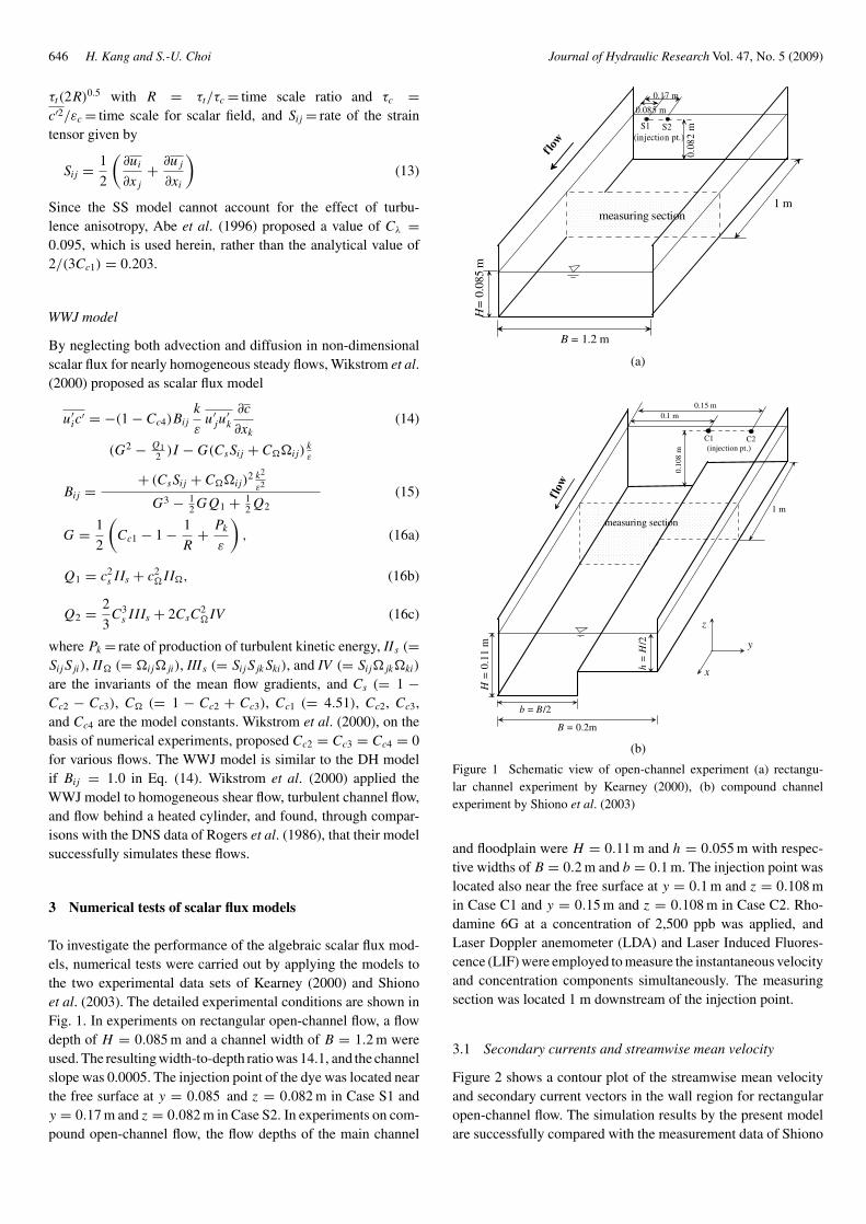
To investigate the performance of the algebraic scalar flux mod-els, numerical tests were carried out by applying the models tothe two experimental data sets of Kearney (2000) and Shionoet al. (2003). The detailed experimental conditions are shown inFig. 1. In experiments on rectangular open-channel flow, a flowdepth of H = 0.085 m and a channel width of B = 1.2 m wereused. The resulting width-to-depth ratio was 14.1, and the channelslope was 0.0005. The injection point of the dye was located nearthe free surface at y = 0.085 and z = 0.082 m in Case S1 andy = 0.17 m and z = 0.082 m in Case S2. In experiments on com-pound open-channel flow, the flow depths of the main channel

H=

0.08

5 m

B = 1.2 m

1 mmeasuring section

0.085 m

0.17 m

S1 S2(injection pt.)

0.08

2 m

f low

(a)

(b)

H =

0.1

1m

h =

H/2

b = B/2

B = 0.2m

x

y

z

measuring section

(injection pt.)C1 C2

0.10

8 m

0.1 m0.15 m

1 m

f low

Figure 1 Schematic view of open-channel experiment (a) rectangu-lar channel experiment by Kearney (2000), (b) compound channelexperiment by Shiono et al. (2003)

and floodplain were H = 0.11 m and h = 0.055 m with respec-tive widths of B = 0.2 m and b = 0.1 m. The injection point waslocated also near the free surface at y = 0.1 m and z = 0.108 min Case C1 and y = 0.15 m and z = 0.108 m in Case C2. Rho-damine 6G at a concentration of 2,500 ppb was applied, andLaser Doppler anemometer (LDA) and Laser Induced Fluores-cence (LIF) were employed to measure the instantaneous velocityand concentration components simultaneously. The measuringsection was located 1 m downstream of the injection point.

3.1 Secondary currents and streamwise mean velocity

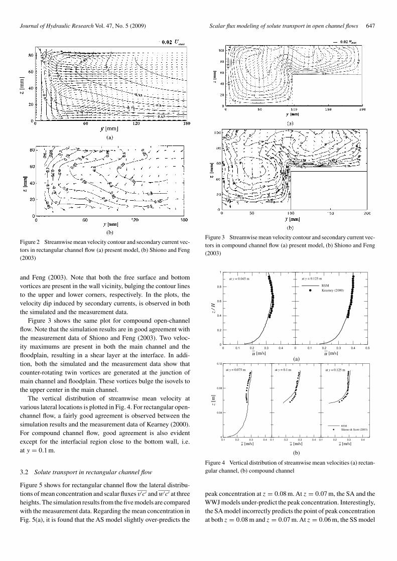
Figure 2 shows a contour plot of the streamwise mean velocityand secondary current vectors in the wall region for rectangularopen-channel flow. The simulation results by the present modelare successfully compared with the measurement data of Shiono


Figure 2 Streamwise mean velocity contour and secondary current vec-tors in rectangular channel flow (a) present model, (b) Shiono and Feng(2003)

and Feng (2003). Note that both the free surface and bottomvortices are present in the wall vicinity, bulging the contour linesto the upper and lower corners, respectively. In the plots, thevelocity dip induced by secondary currents, is observed in boththe simulated and the measurement data.

Figure 3 shows the same plot for compound open-channelflow. Note that the simulation results are in good agreement withthe measurement data of Shiono and Feng (2003). Two veloc-ity maximums are present in both the main channel and thefloodplain, resulting in a shear layer at the interface. In addi-tion, both the simulated and the measurement data show thatcounter-rotating twin vortices are generated at the junction ofmain channel and floodplain. These vortices bulge the isovels tothe upper center in the main channel.

The vertical distribution of streamwise mean velocity atvarious lateral locations is plotted in Fig. 4. For rectangular open-channel flow, a fairly good agreement is observed between thesimulation results and the measurement data of Kearney (2000).For compound channel flow, good agreement is also evidentexcept for the interfacial region close to the bottom wall, i.e.at y = 0.1 m.

3.2 Solute transport in rectangular channel flow

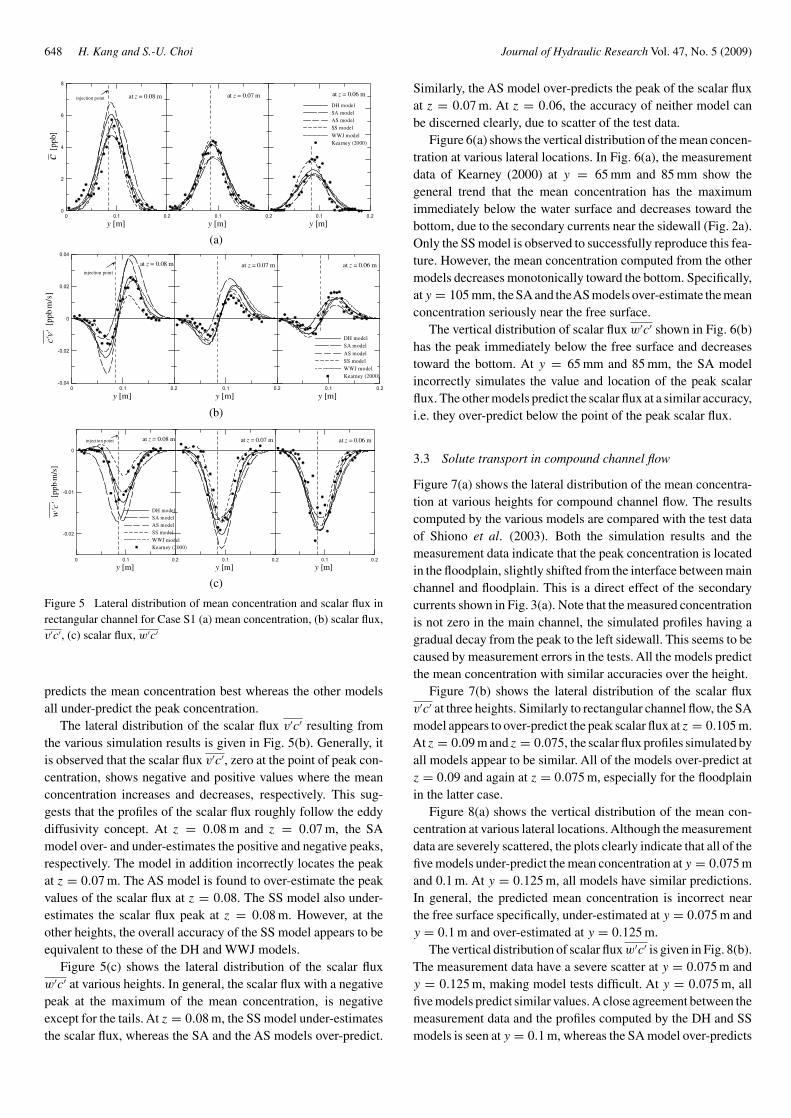
Figure 5 shows for rectangular channel flow the lateral distribu-tions of mean concentration and scalar fluxes v′c′ and w′c′ at threeheights. The simulation results from the five models are comparedwith the measurement data. Regarding the mean concentration inFig. 5(a), it is found that the AS model slightly over-predicts the

Figure 3 Streamwise mean velocity contour and secondary current vec-tors in compound channel flow (a) present model, (b) Shiono and Feng(2003)

0 0.1 0.2 0.3 0.4

u [m/s]

0

0.2

0.4

0.6

0.8

1

z /

H

0 0.1 0.2 0.3 0.4 0.5

u [m/s]

RSMKearney (2000)

at y = 0.045 m at y = 0.125 m

(a)

0.1 0.2 0.3 0.4

u [m/s]

0

0.04

0.08

0.12

z [m

]

0.1 0.2 0.3 0.4

u [m/s]0.1 0.2 0.3 0.4

u [m/s]

RSMShiono & Scott (2003)

at y = 0.125 mat y = 0.075 m at y = 0.1 m

(b)

Figure 4 Vertical distribution of streamwise mean velocities (a) rectan-gular channel, (b) compound channel

peak concentration at z = 0.08 m. At z = 0.07 m, the SA and theWWJ models under-predict the peak concentration. Interestingly,the SA model incorrectly predicts the point of peak concentrationat both z = 0.08 m and z = 0.07 m. At z = 0.06 m, the SS model


0 0.1 0.2

y [m]

0

2

4

6

8

c [p

pb]

DH modelSA modelAS modelSS modelWWJ modelKearney (2000)

0.1 0.2

y [m]0.1 0.2

y [m]

at z = 0.06 mat z = 0.07 mat z = 0.08 minjection point

(a)

0 0.1 0.2

y [m]

-0.04

-0.02

0

0.02

0.04

c'v'

[ppb

⋅m/s

]


0.1 0.2

y [m]0.1 0.2

y [m]


(b)

0 0.1 0.2

y [m]

-0.02

-0.01

0

w'c

' [p

pb⋅m

/s]


0.1 0.2

y [m]0.1 0.2

y [m]


(c)

Figure 5 Lateral distribution of mean concentration and scalar flux inrectangular channel for Case S1 (a) mean concentration, (b) scalar flux,v′c′, (c) scalar flux, w′c′

predicts the mean concentration best whereas the other modelsall under-predict the peak concentration.

The lateral distribution of the scalar flux v′c′ resulting fromthe various simulation results is given in Fig. 5(b). Generally, itis observed that the scalar flux v′c′, zero at the point of peak con-centration, shows negative and positive values where the meanconcentration increases and decreases, respectively. This sug-gests that the profiles of the scalar flux roughly follow the eddydiffusivity concept. At z = 0.08 m and z = 0.07 m, the SAmodel over- and under-estimates the positive and negative peaks,respectively. The model in addition incorrectly locates the peakat z = 0.07 m. The AS model is found to over-estimate the peakvalues of the scalar flux at z = 0.08. The SS model also under-estimates the scalar flux peak at z = 0.08 m. However, at theother heights, the overall accuracy of the SS model appears to beequivalent to these of the DH and WWJ models.

Figure 5(c) shows the lateral distribution of the scalar fluxw′c′ at various heights. In general, the scalar flux with a negativepeak at the maximum of the mean concentration, is negativeexcept for the tails. At z = 0.08 m, the SS model under-estimatesthe scalar flux, whereas the SA and the AS models over-predict.

Similarly, the AS model over-predicts the peak of the scalar fluxat z = 0.07 m. At z = 0.06, the accuracy of neither model canbe discerned clearly, due to scatter of the test data.

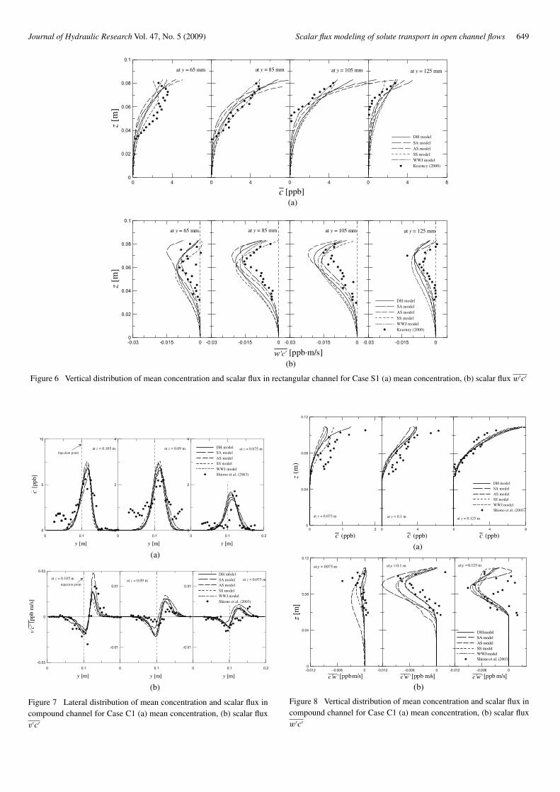
Figure 6(a) shows the vertical distribution of the mean concen-tration at various lateral locations. In Fig. 6(a), the measurementdata of Kearney (2000) at y = 65 mm and 85 mm show thegeneral trend that the mean concentration has the maximumimmediately below the water surface and decreases toward thebottom, due to the secondary currents near the sidewall (Fig. 2a).Only the SS model is observed to successfully reproduce this fea-ture. However, the mean concentration computed from the othermodels decreases monotonically toward the bottom. Specifically,aty = 105 mm, the SA and theAS models over-estimate the meanconcentration seriously near the free surface.

The vertical distribution of scalar flux w′c′ shown in Fig. 6(b)has the peak immediately below the free surface and decreasestoward the bottom. At y = 65 mm and 85 mm, the SA modelincorrectly simulates the value and location of the peak scalarflux. The other models predict the scalar flux at a similar accuracy,i.e. they over-predict below the point of the peak scalar flux.

3.3 Solute transport in compound channel flow

Figure 7(a) shows the lateral distribution of the mean concentra-tion at various heights for compound channel flow. The resultscomputed by the various models are compared with the test dataof Shiono et al. (2003). Both the simulation results and themeasurement data indicate that the peak concentration is locatedin the floodplain, slightly shifted from the interface between mainchannel and floodplain. This is a direct effect of the secondarycurrents shown in Fig. 3(a). Note that the measured concentrationis not zero in the main channel, the simulated profiles having agradual decay from the peak to the left sidewall. This seems to becaused by measurement errors in the tests. All the models predictthe mean concentration with similar accuracies over the height.

Figure 7(b) shows the lateral distribution of the scalar fluxv′c′ at three heights. Similarly to rectangular channel flow, the SAmodel appears to over-predict the peak scalar flux at z = 0.105 m.At z = 0.09 m and z = 0.075, the scalar flux profiles simulated byall models appear to be similar. All of the models over-predict atz = 0.09 and again at z = 0.075 m, especially for the floodplainin the latter case.

Figure 8(a) shows the vertical distribution of the mean con-centration at various lateral locations. Although the measurementdata are severely scattered, the plots clearly indicate that all of thefive models under-predict the mean concentration at y = 0.075 mand 0.1 m. At y = 0.125 m, all models have similar predictions.In general, the predicted mean concentration is incorrect nearthe free surface specifically, under-estimated at y = 0.075 m andy = 0.1 m and over-estimated at y = 0.125 m.

The vertical distribution of scalar flux w′c′ is given in Fig. 8(b).The measurement data have a severe scatter at y = 0.075 m andy = 0.125 m, making model tests difficult. At y = 0.075 m, allfive models predict similar values. A close agreement between themeasurement data and the profiles computed by the DH and SSmodels is seen at y = 0.1 m, whereas the SA model over-predicts


0 40

0.02

0.04

0.06

0.08

0.1

z [m

]

0 4 0 4 0 4 8


c [ppb]

at y = 65 mm at y = 85 mm at y = 105 mm at y = 125 mm

(a)

-0.03 -0.015 00

0.02

0.04

0.06

0.08

0.1

z [m

]

-0.03 -0.015 0 -0.03 -0.015 0 -0.03 -0.015 0


w'c' [ppb⋅m/s]

at y = 65 mm at y = 85 mm at y = 105 mm at y = 125 mm

(b)

Figure 6 Vertical distribution of mean concentration and scalar flux in rectangular channel for Case S1 (a) mean concentration, (b) scalar flux w′c′

0 0.1

y [m]

0

5

10

c [

ppb]

DH modelSA modelAS modelSS modelWWJ modelShiono et al. (2003)

0 0.1

y [m]

0

2

4

0 0.1 0.2

y [m]

0

2

4

injection pointat z = 0.105 m at z = 0.09 m at z = 0.075 m

(a)

0 0.1

y [m]

-0.03

0

0.03

v'c'

[pp

bm

/s]


0 0.1

y [m]

-0.01

0

0.01

0 0.1 0.2

y [m]

-0.01

0

0.01injection point

at z = 0.105 m at z = 0.09 m at z = 0.075 m

(b)

Figure 7 Lateral distribution of mean concentration and scalar flux incompound channel for Case C1 (a) mean concentration, (b) scalar fluxv′c′

0 1 2

c (ppb)

0

0.04

0.08

0.12

z (m

)

0 4

c (ppb)0 4 8

c (ppb)


at y = 0.075 m at y = 0.1 m at y = 0.125 m

(a)

-0.012 -0.006 0

c’w’ [ppb m/s]

0

0.04

0.08

0.12

z [m

]

-0.012 -0.006 0

c’w’ [ppb m/s]-0.012 -0.006 0

c’w’ [ppb m/s]


aty = 0.075 m aty = 0.1 m aty = 0.125 m

(b)

Figure 8 Vertical distribution of mean concentration and scalar flux incompound channel for Case C1 (a) mean concentration, (b) scalar fluxw′c′


the scalar flux. At y = 0.125 m, all models except SS predictsimilarly. The scalar flux computed by the SS model appears tobe different from the others near the free surface.

3.4 Accuracy of scalar flux models

The previously simulated profiles revealed the general features ofeach model. To assess the accuracy of each model quantitatively,the discrepancy ratios between the prediction and measurementdata are calculated. The mean discrepancy ratio is defined as

Me = 10b (17a)

where

b = 1

N

∑∣∣∣∣log

(�comp

�meas

)∣∣∣∣ (17b)

In Eq. (17), Me = discrepancy ratio, N = number of data, and�comp and �meas = computed results and the measurement data,respectively. A smaller value of discrepancy ratio reflects a closeragreement between the computed results and the measurementdata.

Table 1 lists the computed discrepancy ratios. The first threecolumns include the discrepancy ratios from the lateral distribu-tions, and the next two columns those from the vertical distri-butions. The sixth columns list the arithmetic means of the fiveratios. For rectangular channel flows, the DH, SA and AS mod-els appear to predict solute transport accurately. For compoundchannel flows, the discrepancy ratios for the DH and SA modelsare small in both Cases C1 and C2. Over the four tests, the arith-metic means for the SA and DH models are 2.11 and 2.19, respec-tively, indicating that these models perform better than the others.

The quantitative results listed in Table 1 suggest that boththe DH model and the SA model are accurate. The comparisonsin Sections 3.2 and 3.3 indicate, moreover, that the DH modelis capable of accurately predicting the mean concentration and

Table 1 Discrepancy ratio

Model Rectangular (Case S1) Rectangular (Case S2)

Lateral Vertical Mean Lateral Vertical Mean

c v′c′ w′c′ c w′c′ c v′c′ w′c′ c w′c′

DH 1.88 2.36 2.43 1.78 2.74 2.23 1.64 2.02 2.46 1.74 3.64 2.30SA 1.86 2.89 2.57 1.98 2.21 2.30 1.51 2.32 1.92 1.48 2.96 2.04AS 1.54 2.72 2.72 2.13 2.36 2.29 2.10 2.21 2.63 1.51 3.07 2.30SS 2.58 2.38 3.99 1.61 2.69 2.65 2.3 2.48 3.11 2.07 4.07 2.81WWJ 1.81 2.63 2.41 1.78 2.93 2.31 1.54 2.37 2.12 1.84 3.9 2.35

Model Compound (Case C1) Compound (Case C2) Mean

Lateral Vertical Mean Lateral Mean

c v′c′ c w′c′ c v′c′

DH 1.68 2.88 2.09 1.74 2.09 1.60 2.34 1.97 2.19SA 1.55 2.82 1.97 2.12 2.11 1.77 1.83 1.80 2.11AS 2.12 2.93 2.04 1.86 2.23 1.69 2.63 2.16 2.26SS 1.62 4.06 1.73 1.70 2.27 1.96 3.00 2.30 2.58WWJ 1.94 4.85 1.86 1.89 2.63 1.73 2.62 2.18 2.39

scalar fluxes. However, although it is true that the discrepancyratio for the SA model is the smallest, the SA model incorrectlypredicts the location of peak concentration and over-predicts thescalar flux (Fig. 5). Moreover, the SA model is more complicatedthan the DH model, suggesting that the latter is the best choicefor predicting solute transport in open-channel flows.

4 Impact of secondary currents

Figure 9 shows simulated contour plots of the mean concen-tration, together with secondary current vectors for Case S1 atvarious longitudinal locations. Herein, the DH model is used forcomputation. A gradual dilution in the streamwise direction ofdye injected at x = 0 is seen. At x = 3 m, the dye reaches thesidewalls as well as the bottom, showing contour lines bulged tothe lower left corner, whereas at x = 1 m the concentration distri-bution is almost symmetric. This asymmetry is due to secondarycurrents formed for 0.5 < z/H < 0.8, where the free surface andthe bottom vortices merge and head to the left sidewall. The sec-ondary currents also affect the point of the peak concentration,shifting it slightly to the right; however, their impact is hardlynoticeable.

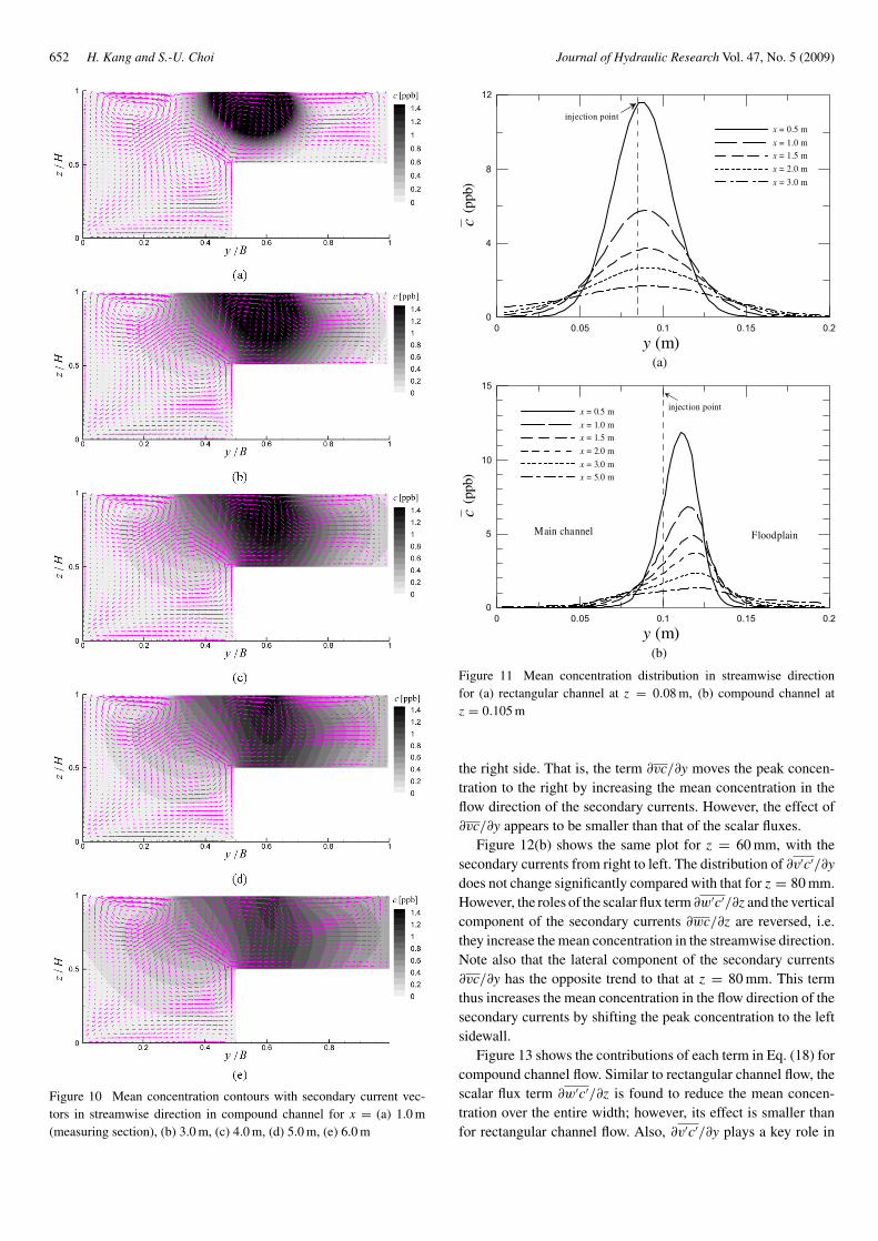
Figure 10 shows the same contour plots for the compoundchannel flow (Case C1). Compared with Fig. 9, a shift of thepeak concentration point is observed. It appears that the freesurface vortex in the main channel and the twin vortex at thejunction make the contour lines at x = 3 m bulged toward themain channel. Similarly, the secondary currents on the floodplainmake the contour lines bulged to the right sidewall. Comparedwith rectangular channel flow, the impact of the secondary cur-rents is pronounced. This is not because of the magnitude ofthe secondary currents but because of the location of the injec-tion point. That is, the injection point in compound channel flowis located in the region of the strong secondary currents. For


Figure 9 Mean concentration contour with secondary current vectors instreamwise direction in rectangular channel at x = (a) 1.0 m (measuringsection), (b) 3.0 m, (c) 4.0 m, (d) 5.0 m, (e) 6.0 m

compound channel flow, the simulated maximum magnitude ofthe secondary current vectors is 2.9% of the maximum veloc-ity, which is not significantly higher than 2.07% for rectangularchannel flow.

Figure 11(a) shows the lateral distribution of the mean concen-tration at z = 0.08 m for rectangular channel flow. The locationof the peak concentration at x = 0.5 m is slightly shifted to theright due to secondary currents; however, the impact is hardlynoticeable. The location of the peak concentration is no longermoving beyond x = 1.0 m. In general, the shape of the meanconcentration observed is of Gaussian distribution. However, thedistribution beyond x = 3.0 m shows the left tail thicker than theright (Fig. 9).

For compound channel flow, the mean concentration at z =0.105 m is shown in Fig. 11(b). The figure clearly depicts the shiftof the location of the peak concentration to the right. A continuousshift is noticeable up to x = 2 m, beyond which its location hardlymoves. The distribution of the mean concentration at x = 5 mbecomes quite uniform in the transverse direction. Unlike forrectangular channel flow, the mean concentration shows a dis-tribution skewed to the left, rather than a Gaussian distribution,which is due to secondary currents. That is, the secondary cur-rents make the mean concentration in the floodplain higher thanin the main channel.

5 Solute transport rate

For steady uniform flows, the scalar transport equation withoutmolecular diffusion takes the form

∂uc

∂x= −

(∂v′c′

∂y+ ∂w′c′

∂z

)− ∂vc

∂y− ∂wc

∂z(18)

Using measured data, Shiono and Feng (2003) investigated theimpacts of Reynolds flux and secondary currents on the solutetransport rate. However, they ignored the vertical component ofthe secondary currents, the fourth term on the right side of Eq.(18) due to test resolution. Herein, a similar analysis is performedusing simulated data, including the vertical component.

Figure 12(a) shows the lateral distribution of the magnitudeof each term on the right side of Eq. (18) for rectangular channelflow. It is found that at z = 80 mm, the location of the minimumvalue of ∂v′c′/∂y or ∂w′c′/∂z is similar to that of the peak of themean concentration. At this height, the direction of the secondarycurrents is from left to right. This suggests that these scalar fluxesreduce the mean concentration peak in the streamwise direction.Specifically, ∂w′c′/∂z reduces the mean concentration over theentire width. In contrast, ∂v′c′/∂y reduces the peak concentrationin the middle of the channel, while it increases the concentrationat the tails. Additionally, the vertical component of the secondarycurrents ∂wc/∂z decreases the mean concentration over the entirewidth; however, its effect is small compared with the scalar fluxes.It is also noteworthy the lateral component of the secondary cur-rents ∂vc/∂y reduces the mean concentration on the left side ofthe injection point, while it increases the mean concentration on


Figure 10 Mean concentration contours with secondary current vec-tors in streamwise direction in compound channel for x = (a) 1.0 m(measuring section), (b) 3.0 m, (c) 4.0 m, (d) 5.0 m, (e) 6.0 m

0 0.05 0.1 0.15 0.2

y (m)

0

4

8

12

c(p

pb)

x = 0.5 m

x = 1.0 mx = 1.5 m

x = 2.0 m

x = 3.0 m

injection point

(a)

0 0.05 0.1 0.15 0.2

y (m)

0

5

10

15

c(p

pb)

x = 0.5 m

x = 1.0 mx = 1.5 m

x = 2.0 m

x = 3.0 mx = 5.0 m

Main channel Floodplain

injection point

(b)

Figure 11 Mean concentration distribution in streamwise directionfor (a) rectangular channel at z = 0.08 m, (b) compound channel atz = 0.105 m

the right side. That is, the term ∂vc/∂y moves the peak concen-tration to the right by increasing the mean concentration in theflow direction of the secondary currents. However, the effect of∂vc/∂y appears to be smaller than that of the scalar fluxes.

Figure 12(b) shows the same plot for z = 60 mm, with thesecondary currents from right to left. The distribution of ∂v′c′/∂ydoes not change significantly compared with that for z = 80 mm.However, the roles of the scalar flux term ∂w′c′/∂z and the verticalcomponent of the secondary currents ∂wc/∂z are reversed, i.e.they increase the mean concentration in the streamwise direction.Note also that the lateral component of the secondary currents∂vc/∂y has the opposite trend to that at z = 80 mm. This termthus increases the mean concentration in the flow direction of thesecondary currents by shifting the peak concentration to the leftsidewall.

Figure 13 shows the contributions of each term in Eq. (18) forcompound channel flow. Similar to rectangular channel flow, thescalar flux term ∂w′c′/∂z is found to reduce the mean concen-tration over the entire width; however, its effect is smaller thanfor rectangular channel flow. Also, ∂v′c′/∂y plays a key role in


0 0.05 0.1 0.15 0.2

y / H

-2

-1

0

1

Tra

nspo

rt r

ate

- dv'c' / dy

- dw'c' / dz

- dVC / dy

- dWC / dzinjection point

(a)

0 0.05 0.1 0.15 0.2

y / H

-0.8

-0.4

0

0.4

Tra

nspo

rt r

ate

- dv'c' / dy

- d w'c' / dz

- d VC / dy

- d WC / dzinjection point

(b)

Figure 12 Lateral distribution of solute transport rate in rectangularchannel flow at x = 1 m (a) at z = 80 mm, (b) at z = 60 mm

0.04 0.08 0.12 0.16

y / H

-3

-2

-1

0

1

2

Tra

nspo

rt r

ate

- d v'c' / dy

- dw'c' / dz

- dVC / dy

- dWC / dz

injection point

Figure 13 Lateral distribution of solute transport rate in compoundchannel flow at x = 1 m and z = 105 mm

reducing the peak concentration, increasing the mean concen-tration at the tails. Note that the rate of increase of the meanconcentration in the floodplain is higher than that in the mainchannel. This is consistent with the lateral distribution of themean concentration in Fig. 11. The role of ∂vc/∂y is to increasethe mean concentration on the right side of the peak concentra-tion (at y = 0.11 m) and to decrease the mean concentration on

the left side. The effect, although similar for rectangular chan-nel flow, appears to be significant, indicating that the shift ofthe peak concentration is due to the lateral component of thesecondary currents. The vertical component of the secondarycurrents ∂wc/∂z, opposite to ∂vc/∂y, is found to affect the meanconcentration less than the lateral component.

6 Conclusions

Numerical experiments of various algebraic scalar flux models tonumerically simulate solute transport in open-channel flows arepresented. Five algebraic scalar flux models including Daly andHarlow’s, Abe and Suga’s, Suga and Abe’s, Sommer and So’s,and Wikstrom et al.’s were tested. The models were applied tolaboratory measurements of solute transport in the rectangularand compound open-channel flows. To compute the flow, theReynolds stress model of Kang and Choi was used.

For solute transport in rectangular channel flow, simulatedlateral distributions of the mean concentration and scalar fluxeswere compared with measured data. The results suggested thatthe performance of the DH model is best and those of the SSand WWJ models are moderate. For solute transport in com-pound channel flow, the DH, SS, and WWJ models predict thelateral distributions of the mean concentration and scalar fluxrather accurately, though the measurement data showed severescattering. With regard to the vertical distributions, the predic-tions with the DH and WWJ models were relatively accurate. Thediscrepancy ratio between predicted and measured profiles alsosupported that the DH model is best for numerical simulations ofsolute transport in open-channel flows.

On the basis of the mean concentration profiles simulated bythe DH model, the impact of the secondary currents on the solutetransport was investigated. It was observed that the secondarycurrents in the compound channel flow clearly move the loca-tion of peak concentration to the floodplain. This resulted in askewed distribution of the mean concentration in the streamwisedirection. A similar but significantly weak impact was noticed inthe rectangular channel. This is because the dye was injected intothe region where the secondary currents are weak, not because themagnitude of the secondary currents is weaker in the rectangularthan that in the compound channel flow.

With reference to the simulation results, the roles of theReynolds flux and the secondary currents in solute transportwere investigated. For both rectangular and compound channelflows, it was found that the Reynolds fluxes reduce the peak andthicken the tails of the mean concentration. It also was discoveredthat the secondary currents affect the magnitude of the mean con-centration over the entire width, moving the peak concentrationin the flow direction. However, their impact was weak comparedwith that of the Reynolds fluxes.

Acknowledgements

This work was supported by a grant (Code # ’06 CTIP B-01)from the Construction Technology Innovation Program (CTIP)


funded by the Ministry of Land, Transport and Maritime Affairsof Korean government.

Notation

B = Channel widthBc = Buoyancy production

c, c′ = Mean and fluctuating componentsof the concentration

C = Model constantsDic = Turbulent diffusive transportDij = Transport of Rij by diffusiongi = Gravitational accelerationH = Flow depthk = Turbulent kinetic energy

Me = Discrepancy ratioN = Number of datap = Mean pressure

Pc = Mean field productionPk = Rate of turbulent kinetic energy

productionR = Time scale ratio

Sij = Rate of strain tensoru′

i and u′i = Mean and fluctuating velocity

componentsu′

ic′ = Scalar flux

−u′iu

′j (= Rij) = Reynolds stress per unit fluid density

x, y, and z = Longitudinal, transverse, andvertical coordinates

Greek Symbolsε = Dissipation rate of k

εic = Viscous destructionεij = Rate of dissipation of Rij

λ = Molecular diffusivityν and νt = Kinematic and eddy viscosity,

respectively�ij = Rotation tensor�ic = Pressure-scalar gradient correlation�ij = Transport of Rij

�comp and �meas = Computed results and test dataρ = Fluid densityσt = Turbulent Schmidt numberτc = Time scale for scalar field

τm and τt = Characteristic time, andIIs, II�, IIIs, and IV = Invariants of mean flow gradients

References

Abe, K. (2006). Performance of Reynolds-averaged turbu-lence and scalar-flux models in complex turbulence with flowimpingement. Progress in Comput. Fluid Dyn. 6, 79–88.

Abe, K., Kondoh, T., Nagano, Y. (1996). A two-equation heattransfer model reflecting second-moment closures for wall andfree turbulent flows. Intl. J. Heat Fluid Flow 17, 228–237.

Abe, K., Suga, K. (2001a). Large eddy simulation of passivescalar in complex turbulence with flow impingement and flowseparation. Heat Transfer Asian Research 30, 402–418.

Abe, K., Suga, K. (2001b). Towards the development of aReynolds-averaged algebraic turbulent scalar-flux model. Intl.J. Heat Mass Transfer 22, 19–29.

Choi, S.-U., Kang, H. (2001). Numerical tests of Reynolds stressmodels in the computations of open-channel flows. Proc. 8thFlow Modeling and Turbulence Measurements, 71–78, Tokyo,Japan.

Craft, T.J. (1991). Computational modeling of turbulent scalartransport. Report TFD/91/3. Department of Mechanical Engi-neering, UMIST, Manchester UK.

Daly, B.J., Harlow, F.H. (1970). Transport equations in turbu-lence. Phys. Fluids 13, 2634–2649.

Djordjevic, S. (1993). Mathematical model of unsteady transportand its experimental verification in compound channel flow.J. Hydr. Res. 31(2), 229–248.

Gibson, M.M., Launder, B.E. (1978). Ground effects on pressurefluctuations in the atmospheric boundary layer. J. Fluid Mech.86, 491–511.

Hanjalic, K., Launder, B.E. (1972). A Reynolds stress modelof turbulence and its application to thin shear flows. J. FluidMech. 52, 609–638.

Hinterberger, C., Fröhlich, J., Rodi, W. (2007). Three-dimensional and depth-averaged large eddy simulations ofsome shallow water flows. J. Hydr. Engng. 133(8), 857–872.

John, E.C., Williams, J.J.R. (2008). Large eddy simulation of along asymmetric compound open channel. J. Hydr. Res. 46(4),445–453.

Jones, W.P., Musonge, P. (1988). Closure of the Reynolds stressand scalar flux equations. Phys. Fluids 31(12), 3589–3604.

Joung, Y., Choi, S.-U. (2008). Investigation of twin vortices nearthe interface in turbulent open-channel flows using DNS data.J. Hydr. Engng. 134(12), 1744–1756.

Kang, H., Choi, S.-U. (2006a). Reynolds stress modeling of rect-angular open channel flows. Intl. J. Num. Meth. Fluids 51(11),1319–1334.

Kang, H., Choi, S.-U. (2006b). Turbulence modeling of com-pound open-channel flows with and without vegetated flood-plains using the Reynolds stress model. Advances WaterResources 29(11), 1650–1664.

Kearney, D.J. (2000). Turbulent diffusion in channels of complexgeometry. PhD Thesis. Loughbough University, LeicestershireUK.

Kim, J., Moin, P. (1989). Transport of passive scalars in a turbu-lent channel flows. Turbulent Shear Flows, 6, 85–96. Springer,Berlin.

Li, C.W., Wang, J.H. (2000). Large eddy simulation of free sur-face shallow water flow. Intl. J. Numer. Meth. Fluids 34(1),31–46.

Lien, F.S., Leschziner, M.A. (1993). Modelling 2D and 3D sep-aration from curved surfaces with variants of second momentclosure combined with low-Re near-wall formulations. Proc.9th Symp. Turbulent Shear Flows 2, 13–1.


Lin, B., Shiono, K. (1995). Numerical modeling of solutetransport in compound channel flows. J. Hydr. Res. 33(6),773–788.

Mellor, G.L., Herring, H.J. (1973). A survey of mean turbulentfield closure. AIAA J. 11, 590–599.

Murakami, S., Mochida, A., Ooka, R. (1993). Numerical sim-ulation of flow field over surface-mounted cube with varioussecond moment closure models. Proc. 9th Symp. TurbulentShear Flows 2, 13–5.

Nokes, R.I., Hughes, G.O. (1994). Turbulent mixing in uniformchannels of irregular cross section. J. Hydr. Res. 32(1), 67–86.

Peng, S.-H., Davidson, L. (1999). Computation of turbulentbuoyant flows in enclosures with low-Reynolds number k–ω

models. Intl. J. Heat Fluid Flow 20(2), 172–184.Pezzinga, G. (1994). Velocity distribution in compound chan-

nel flows by numerical modeling. J. Hydr. Engng. 120(10),1176–1198.

Prinos, P. (1992). Dispersion in compound open channel flow.Hydraulic and environmental modeling: Estuarine and riverwaters, 359–372, R.A. Falconer, K. Shiono, R.G.S. Mattew,eds. Ashgate, Aldershot UK.

Rogers, M.M., Moin, P., Reynolds, W.C. (1986). The structureand modeling of the hydrodynamic and passive scalar fieldsin homogeneous turbulent shear flow. Dept. Mech. Engng.Report TF-25. Stanford University, Stanford CA.

Rogers, M.M., Mansour, N.N., Reynolds, W.C. (1989). An alge-braic model for the turbulent flux of a passive scalar. J. FluidMech. 203, 77–101.

Rokni, M., Gatski, T. (2001). Predicting turbulent convectiveheat transfer in fully developed duct flows. Intl. J. Heat FluidFlow 22(4), 381–392.

Rokni, M., Sunden, B. (1998). 3D numerical investigation ofturbulent forced convection in wavy ducts with trapezoidalcross-section. Intl. J. Num. Meth. Heat and Fluid Flow 8(1),118–141.

Rotta, J.C. (1951). Statistische Theorie nichthomogener Turbu-lenz. Zeitschrift Physik, 129, 547–572 [in German].

Shih, T.H., Lumley, J.L. (1985). Modeling of pressure cor-relation terms in Reynolds stress and scalar flux equations.Report FDA-85-3. Sibley School of Mechanical andAerospaceEngineering, Cornell University, Ithaca NY.

Shikazono, N., Kasagi, N. (1996). Second-moment closure forturbulent scalar transport at various Prandtl numbers. Intl. J.Heat Mass Transfer 39(14), 2977–2987.

Shiono, K., Feng, T. (2003). Turbulence measurements of dyeconcentration and effects of secondary flow on distribution inopen channel flows. J. Hydr. Engng. 129(5), 373–384.

Shiono, K., Scott, C.F., Kearney, D. (2003). Predictions ofsolute transport in compound channel using turbulence models.J. Hydr. Res. 41(3), 247–258.

Shir, C.C. (1973). A preliminary study of atmospheric turbulentflow in the idealized planetary boundary layer. J. AtmosphericSci. 30, 1327–1339.

Simoes, F.J.M., Wang, S.S.Y. (1997). Numerical prediction ofthree dimensional mixing in a compound channel. J. Hydr.Res. 35(5), 619–642.

Sofialidis, D., Prinos, P. (1999). Numerical study of momentumexchange in compound open-channel flow. J. Hydr. Engng.125(2), 152–165.

Sommer, T.P., So, R.M.C. (1995). On the modeling of homoge-neous turbulence in a stably stratified flow. Phys. Fluids 7(11),2766–2777.

Speziale, C.G., Sarkar, S., Gatski, T. (1991). Modeling the pres-sure strain correlation of turbulence: An invariant dynamicalsystems approach. J. Fluid Mech. 227, 245–272.

Suga, K., Abe, K. (2000). Nonlinear eddy viscosity model-ing for turbulence and heat transfer near wall and shear-freeboundaries. Intl. J. Heat Mass Transfer 21, 37–48.

Thomas, T.G., Williams, J.J.R. (1995). Large eddy simulation ofturbulent flow in a symmetric compound open channel. J. Hydr.Res. 33(1), 27–41.

Wikstrom, P.M., Wallin, S., Johansson, A.V. (2000). Derivationand investigation of a new explicit algebraic model for thepassive scalar flux. Phys. Fluids 12(3), 688–702.

Yoshizawa, A. (1988). Statistical modeling of passive scalardiffusion in turbulent shear flows. J. Fluid Mech. 195,541–555.

Zedler, E.A., Street, R. (2001). Large eddy simulation of sedi-ment transport: Currents over ripples. J. Hydr. Engng. 127(6),444–452.

scalar ﬂux modeling of solute transport in open channel ...envhydro.yonsei.ac.kr/labnews/scalr...

Documents