scenario reduction for risk-averse stochastic programs · bayraksan, and homem-de mello ......
TRANSCRIPT

Scenario Reduction for Risk-Averse Stochastic Programs
Sebastián Arpón∗1, Tito Homem-de-Mello †1, Bernardo Pagnoncelli‡1
1School of Business, Universidad Adolfo Ibañez, Santiago, Chile
Abstract
In this paper we discuss scenario reduction methods for risk-averse stochastic optimizationproblems. Scenario reduction techniques have received some attention in the literature andare used by practitioners, as such methods allow for an approximation of the random variablesin the problem with a moderate number of scenarios, which in turn make the optimizationproblem easier to solve. The majority of works for scenario reduction are designed for classicalrisk-neutral stochastic optimization problems; however, it is intuitive that in the risk-averse caseone is more concerned with scenarios that correspond to high cost. By building upon the notionof effective scenarios recently introduced in the literature, we formalize that intuitive idea andpropose a scenario reduction technique for stochastic optimization problems where the objectivefunction is a Conditional Value-at-Risk. The numerical results presented with problems fromthe literature illustrate the performance of the method and indicates the general cases where weexpect it to perform well.
1 Introduction
Scenario generation and scenario reduction methods have a long history in stochastic programming.The importance of such methods stems from the need to approximate the (joint) probability distri-bution of the random variables in the problem with another distribution with a moderate numberof outcomes — henceforth called scenarios — so that the resulting optimization problem can beefficiently solved, perhaps by means of some algorithm that decomposes the problem across scenar-ios. Here we make a distinction between scenario generation and scenario reduction: in the former,scenarios are chosen from the original distributions, whereas the latter starts with a finite set ofscenarios and attempts to find a smaller subset. In both cases the goal is the same — to obtainan approximating problem that provides a good approximation to the original one. We will discussshortly what is meant by a “good approximation".
Many approaches for scenario generation/reduction have been developed in the literature. Theseinclude, for example, clustering (e.g., Dupačová, Consigli, andWallace (2000)) and moment-matchingtechniques, see Hoyland and Wallace (2001); Hoyland, Kaut, and Wallace (2003) and Mehrotra andPapp (2014). Another approach is based on generating scenarios via sampling from the underlyingprobability distributions, as in the case of the Sample Average Approximation (SAA) approach;overviews of sampling-based methods together with their properties can be found in Shapiro (2003)and Homem-de-Mello and Bayraksan (2014).∗[email protected]†[email protected]; Corresponding author‡[email protected]
1

Another class of methods, based on probability metrics, aims at finding a distribution Q withrelatively few scenarios in such a way that Q minimizes a distance d(P,Q) between Q and theoriginal distribution P . Typically, these approaches rely on stability results that ensure that thedifference between the optimal values of the original and approximating problems is bound by aconstant times d(P,Q). Several distances for distributions can be used for that purpose, such as theWasserstein distance and the Fortet-Mourier metric. This type of approach has gained attentionespecially for the case of multistage problems, where the goal is to derive a scenario tree that properlyapproximates the original problem, though more sophisticated distances are required in that case.We refer to (Pflug, 2001; Dupačová, Gröwe-Kuska, & Römisch, 2003; Heitsch & Römisch, 2003,2009; Pflug & Pichler, 2011) and references therein for further discussions on this type of methods.
The vast majority of scenario generation/reduction methods found in the literature assume thatthe underlying optimization problem has the form
minx∈X
E [G(x, ξ)] , (1.1)
where ξ is a random vector representing the uncertainty in the problem, and G is a cost functionthat depends on ξ as well as on the decision variables x (we shall assume, as customary in theliterature, that G is convex in x and X is a convex closed set). Such a formulation assumes thatthe decision-maker is risk-neutral, i.e., large losses in one scenario can be offset by large gains inanother one. In many situations, however, the decision-maker is risk-averse and wants to protectagainst the risk of (large) losses. Such problems are modeled by replacing the expectation in (1.1)with a proper risk measure. Optimization problem with risk aversion have been extensively studiedin the literature in the past 10-20 years, both from theoretical and application perspectives.
The “explosion" of papers in risk-averse optimization, however, has not been accompanied bya similar effort in the scenario generation/reduction literature. This is due in part to the factthat some risk measures can be written in terms of expectations; a prominent example is theConditional-Value-at-Risk (CVaR), also called Average-Value-at-Risk, which we review briefly herefor completeness and to set up some notation that will be used throughout the paper. The Valueat Risk (VaR) of a random variable Z with cdf F (·) with risk level α ∈ [0, 1] is defined as
VaRα[Z] := min{t | F (t) ≥ α} = min{t | P (Z ≤ t) ≥ α}. (1.2)
The Conditional Value-at-Risk (CVaR) of a random variable Z with cdf F (·) with risk level α ∈ [0, 1]is defined as
CVaRα[Z] :=1
1− α
∫ 1
αVaRγ [Z]dγ. (1.3)
A key result in Rockafellar and Uryasev (2000) is the proof that CVaR can be expressed as theoptimal value of the following optimization problem:
CVaRα[Z] = minη∈R
{η +
1
1− αE [(Z − η)+]
}, (1.4)
where (a)+ := max(a, 0). Moreover, they show that VaRα[Z] is an optimal solution of the opti-mization problem in (1.4). 1
Suppose now that that we want to solve a CVaR-version of problem (1.1), i.e.,
minx∈X
CVaRα [G(x, ξ)] . (1.5)
1A useful property of CVaRα that will be used in the sequel is that it coincides with the expectation when α = 0.Moreover, limα→1 CVaRα[Z] = ess sup (Z).
2
Such problems have received considerable attention in the literature, starting with the seminal workby Rockafellar and Uryasev (2000); see also Miller and Ruszczynski (2011) for the case where theproblem is a two-stage stochastic program, and Noyan (2012) and Pineda and Conejo (2010) for dis-cussions of applications of such models in humanitarian logistics and energy planning, respectively2.Then, by using representation (1.4), we can reformulate (1.5) as
minx∈X, η∈R
{η +
1
1− αEP [(G(x, ξ)− η)+]
}. (1.6)
We see that (1.6) is an optimization problem with expectations, though in an extended space. Thus,we can in principle apply any of the scenario generation/reduction techniques discussed earlier.Note also that formulation (1.6) makes it explicit the underlying distribution P used to calculatethe CVaR in (1.5).
A closer look at the objective function in (1.6), however, shows why standard scenario gen-eration/reduction methods may not work so well in that context. To see that, observe firstthat for any given x, the optimal η = η(x) is given by η(x) = VaRα [G(x, ξ)]; see Rockafellarand Uryasev (2000). Also, for any fixed x, the value of E [(G(x, ξ)− η(x))+] is zero for all sce-narios ξ such that G(x, ξ) ≤ η(x), so such scenarios do not contribute to the calculation. Inparticular, at an optimal solution (x∗, η∗) to (1.6) we have that only the scenarios ξ such thatG(x∗, ξ) > η(x∗) = VaRα [G(x∗, ξ)] contribute to the optimal objective function value. So, onecould argue that generating scenarios outside the tail of G(x∗, ·) is actually wasteful.
As presented, the above argument is of course heuristic and raises many questions. For example,while it is true that a scenario ξ such that G(x∗, ξ) ≤ η(x∗) does not contribute to the optimalobjective function value, it could certainly be the case that G(x, ξ) > η(x)) for values of x 6= x∗, inwhich case ξ does contribute to the evaluation of the objective function outside the optimal solution— so it is not clear whether such ξ can really be discarded. Nevertheless, the idea that only thescenarios “in the tail" must be generated has gained some traction in the literature, often in aheuristic way; examples are Pineda and Conejo (2010) and García-Bertrand and Mínguez (2014).Fairbrother, Turner, and Wallace (2015) provide a more solid argument by defining precisely thenotion of risk regions. We review these works in more detail in Section 3.
In this paper we present a scenario reduction method for risk-averse problems of the form (1.5),in which the distribution of the underlying random vector ξ has finite support Ξ := {ξ1, . . . , ξn} witha moderately large number of elements. A typical situation where this occurs is when a large randomsample is drawn from the original distribution in order to represent that distribution well. We callit the source distribution and will represent it by P , with Pi denoting the probability of scenarioξi. One then aims at reducing the number of scenarios of the source distribution further so thatthe optimization problem can be solved in a reasonable time. While our work has some similaritieswith the aforementioned papers that address the same problem — in the sense that we also aimat generating scenarios in the tail of G(x, ·) — we define precisely what is the set of scenarios thatmatter for the problem and how to generate a representative subset of those scenarios.
Our method relies strongly on the concept of effective scenarios recently introduced by Rahimian,Bayraksan, and Homem-de Mello (2018). According to that notion, a scenario is effective if itsremoval from the problem leads to changes in the optimal objective value (there is a precise definitionfor “removal"); otherwise it is called ineffective. Thus, our method tries to (i) identify the ineffectivescenarios for (1.5), as those are provably unnecessary since the optimal value does not change if theyare removed, and (ii) find a distribution whose support is a subset of the set of effective scenarios,and which minimizes the distance to the source distribution.
2Models with CVaR have also been used in the context of multistage stochastic programs, but we do not reviewthem here as we focus on the static case in this paper.
3

We apply our method to the class of two-stage stochastic programs in which randomness appearsonly in the right-hand side. In such cases we are able to provide some heuristic techniques to furtherspeed up the scenario reduction algorithm. We illustrate our methodology with a number of CVaR-versions of problems from the literature, where we compare the results obtained with our methodto those obtained with traditional scenario generation techniques. The comparisons show that ourapproach typically performs well, in some cases it yields a much more accurate solution for the samenumber of scenarios.
2 Background material
In this section, for the sake of completeness — and to set up some notation — we review someconcepts from the literature that will be used in the sequel.
2.1 Risk-averse two-stage stochastic programs
Two-stage stochastic programs constitute a fundamental class of problems in the field of stochasticprogramming. In those problems, the decision maker decides in a first stage, then an outcome of arandom variable is revealed and finally another decision is made, which depends on the first stagedecision and the outcome of the random variable. The classical formulation of two-stage stochasticlinear programming with fixed recourse can be written as follows
minx
dᵀx+Q(x),
subject to Ax = b, (2.1)x ≥ 0,
where A ∈ Rr1×s1 , x ∈ Rs1×1, b ∈ Rr1×1, with r1 and s1 representing the number of constraints andvariables of the first stage problem. As stated earlier, the vector ξ is random with known sourcedistribution P (with finite support), so the function Q(x) = EP [Q(x, ξ)] is written as Q(x) =∑n
i=1 PiQ(x, ξi), where Q(x, ξ) is defined as follows3:
Q(x, ξ) = minzξ
qᵀzξ
subject to Wzξ = hξ − T ξx (2.2)zξ ≥ 0.
In the above formulation, Tξ ∈ Rr2×s1 , W ∈ Rr2×s2 , zξ ∈ Rs2×1, hξ ∈ Rr2×1 with r2 and s2 repre-senting the number of constraints and variables of the second stage problem. Two-stage stochasticlinear programs were first proposed by (G. B. Dantzig, 1955), and the theoretical properties of thisclass of problems are well known (for instance, for every fixed ξi the function Q(x, ξi) is convex, andthe function Q(x) is piecewise linear convex, see Birge and Louveaux (2011)). Applications of thesemodels include finance, energy, natural resources, disaster relief, among others; see, for instance,Wallace and Ziemba (2005).
The development of theory of optimization with risk measures have led formulations of risk-averse two-stage models, where the expectation in the function Q(x) = EP [Q(x, ξ)] is replacedwith some other coherent risk measure; see, for instance, Ahmed (2006), Römisch and Wets (2007),
3In the most general case, W anmd q are random as well, but for our purposes we assume that these quantitiesare deterministic.
4

Miller and Ruszczynski (2011), and Noyan (2012). In our case, as mentioned earlier, we considerproblems with Conditional Value-at-Risk. That is, we replace (2.1) with
minx
dᵀx+ CVaRα [Q(x, ξ)]
subject to Ax = b (2.3)x ≥ 0.
Note that because of the translation-invariant property of CVaR (i.e. CVaRα[a + Z] = a +CVaRα[Z]), the above problem fits the frameworlk of (1.5), with G(x, ξ) = dᵀx + Q(x, ξ). More-over, by using formulation (1.4), we can alternatively formulate (2.3) as a standard (risk-neutral)two-stage stochastic program with extra variables, as indicated below:
minx,η,ν
dᵀx+ η + Q(x, η),
subject to Ax = b, (2.4)x ≥ 0,
where Q(x, η) = EP[Q(x, η, ξ)
]and Q(x, η, ξ) is defined as follows:
Q(x, η, ξ) = minzξ,νξ
1
1− ανξ,
subject to Wzξ = hξ − T ξx, (2.5)νξ − qᵀzξ ≥ −η
zξ, νξ ≥ 0,
Note that, once the scenarios are fixed, the above formulation allows us to solve the optimizationproblem using standard decomposition techniques.
2.2 Scenario reduction via the Monge-Kantorovich problem
We review next the approach proposed in Dupačová, Gröwe-Kuska, and Römisch (2003) for scenarioreduction. The idea relies upon the notion of stability of stochastic programs which is extensivelydeveloped in the literature. While we follow the ideas from Dupačová et al. (2003), we present theresults in the context of distributions with finite support, which is the case of the models in thispaper. The restriction to finite distributions allows us to simplify considerably the results and therequired assumptions.
The following assumptions are made regarding problem (1.1): X ⊂ Rn is a given nonemptyconvex closed set, ξ is a random vector with values in Ξ and distribution P , and the function Gfrom Rs × Ξ to the extended real numbers R is lower semicontinuous and convex with respect tox. Moreover, G(·, ξ) is bounded on X for all ξ ∈ Ξ. The optimal value, parameterized by thedistribution of ξ, is denoted by
v(P ) := inf {EP [G(x, ξ)] : x ∈ X} (2.6)
Given the source distribution P and an approximation P , quantitative estimates of the closenessof v(P ) to v(P ) in terms of a certain probability metric can be shown. To proceed, let P(Ξ) denote
5
the set of distributions whose support is contained in Ξ. Define the distance dG,ρ(P, P ) betweentwo probability distributions in P(Ξ) as follows:
dG,ρ(P, P ) := supx∈X∩ρB
∣∣EP [G(x, ξ)]− EP [G(x, ξ)]∣∣ = sup
x∈X∩ρB
∣∣∣∣∣n∑i=1
G(x, ξi)P (ξi)−n∑i=1
G(x, ξi)P (ξi)
∣∣∣∣∣ .In the above expressions, The set B ⊂ Rn is the ball centered in the origin with radius equals to 1.
By relying on results in (Rockafellar & Wets, 1998), Dupačová et al. (2003) show that thereexist constants ρ > 0 and ε > 0 such that∣∣∣v(P )− v(P )
∣∣∣ ≤ dG,ρ(P, P ) (2.7)
whenever P ∈ P(Ξ) with dG,ρ(P, P ) < ε. Notice that a major consequence of (2.15) is that, if wehave a new distribution P that is close enough to the source distribution P , then the differencesbetween both objective function values will be bounded by the distance between both distributions.Thus, if we can find a new distribution P ∈ P(Ξ) which has smaller support than P but is sufficientlyclose to P , then we obtain a problem which is easier to solve than (1.1) and provides a goodapproximation to that problem in terms of optimal values.
As we can see from the definition, it is very hard to compute the value of dG,ρ(P, P ) which isrequired to verify (2.7). It is possible however to derive upper bounds for that quantity in termsof P and P . To do so, suppose we have a function c : Ξ × Ξ 7→ R+ that provides a “distance"between two scenarios ξ and ξ ∈ Ξ. The function c does not necessarily represent a distance; it isonly required that (i) c be symmetric, and (ii) c(ξ, ξ) = 0 if and only if ξ = ξ.
Given the function c described above, suppose that the function G satisfies
|G(x, ξ)−G(x, ξ)| ≤ h(‖x‖) c(ξ, ξ) (2.8)
for some nondecreasing function h : R+ 7→ R++. Since ‖x‖ ≤ ρ for any x ∈ X ∩ ρB, it follows from(2.8) that the function G(·, ξ) := G(·, ξ)/h(ρ) (when restricted to X ∩ ρB) belongs to the class offunctions
Fc :={f : Ξ 7→ R : |f(ξ)− f(ξ)| ≤ c(ξ, ξ)
}(2.9)
and thus by definition of dG,ρ(P, P ) we must have
dG,ρ(P, P ) = h(ρ) supx∈X∩ρB
∣∣∣EP [G(x, ξ)]− EP
[G(x, ξ)
]∣∣∣ ≤ h(ρ) supf∈Fc
(EP [f(ξ)]− EP [f(ξ)]
)(2.10)
(note that we remove the absolute value in the right-most expression since f ∈ Fc implies that−f ∈ Fc).
The key idea now is to show that the right-hand side of (2.10) can be easily computed. Indeed,notice that since Ξ = {ξ1, . . . , ξn}, it follows that we can view each function f : Ξ 7→ R as a vectorin Rn; we write fi for f(ξi) for short, and similarly for the probabilities P (ξi) and P (ξi). Moreover,we can view the function c as a matrix in Rn×n, and write cij for c(ξi, ξj). With this notation,we can see that the “sup" problem on the right-hand side of (2.10) can be formulated as the linearprogram
maxf
n∑k=1
(Pk − Pk) fk (2.11)
s. to |fi − fj | ≤ cij , i, j = 1, . . . , n.
6

The dual of this linear program is given by
minπ
n∑i,j=1
cij πij
s. ton∑j=1
πkj −n∑i=1
πik = Pk − Pk, k = 1, . . . , n (2.12)
π ≥ 0.
These linear programs can be easily solved. Moreover, there is no duality gap, as both primal anddual are feasible; this can be seen by taking fi = a for all i in the primal (where a is any constant),and πij = PiPj in the dual. However, we wish to take a step further to obtain a quantity thatrepresents a distance between P and P . Indeed, consider the linear program below, which is knownas the Monge-Kantorovich mass transportation problem in finite dimensions:
minπ
n∑i,j=1
cij πij
s. ton∑j=1
πkj = Pk, k = 1, . . . , n (2.13)
n∑i=1
πik = Pk, k = 1, . . . , n (2.14)
π ≥ 0.
The optimal value function µc(P, P ) of problem (2.13)-(2.14) is known as the Kantorovich functional.It is useful to observe that in the particular case where c(ξ, ξ) = ‖ξ − ξ‖, the functional µc(P, P )becomes the well-known Wasserstein distance between P and P ; see, for instance, Rachev (1991)for a thorough discussion of these concepts.
By noticing that equation (2.12) can be written by subtracting (2.14) from (2.13), it followsthat the feasibility set of the former problem contains that of the latter one, which implies that theoptimal value of problem (2.12) is less than or equal to µc(P, P ). Together with (2.7) and (2.10),this implies that ∣∣∣v(P )− v(P )
∣∣∣ ≤ dG,ρ(P, P ) ≤ h(ρ) µc(P, P ), (2.15)
The focus of the work Dupačová et al. (2003) can be described as follows: suppose that we havea fixed probability distribution P from a discrete random variable. Then, find a new distributionP with supp(P ) ⊂ Ξ and |supp(P )| = M < n = |Ξ| (where supp(P ) indicates the support ofthe distribution P ), such that P minimizes the optimal value of the Monge-Kantorovich problem
7
(2.13)-(2.14) in its discrete form. This amounts to solving the following problem
minπ,r
n∑i=1
n∑j=1
cijπij
s. ton∑j=1
πij = Pi, i = 1, . . . , n
πij ≤ rj , i, j = 1, . . . , n (2.16)n∑j=1
rj = M
πij ∈ [0, 1] , i, j = 1, . . . , n
rj ∈ {0, 1}, j = 1, . . . , n,
where M is the cardinality of supp(P ). Let (π∗, r∗) be an optimal solution to (2.16). Then, theselected scenarios are those for which r∗j = 1 (call that set R). The probability of each selectedscenario j is given by
Pj =∑i∈Cj
πij , j ∈ R, (2.17)
where Cj is the set of scenarios ξi such that scenario ξj is the “closest" scenario to ξi (in terms ofcij) among those that belong to R.
Since (2.16) is an NP-Hard problem, in Dupačová et al. (2003) develop a so-called backwardrecursion heuristic to solve (2.16). Briefly speaking, the idea of the backward reduction is to reducethe scenarios one by one, as the problem of reducing the cardinality from n to n− 1 can be solvedefficiently. We refer to that paper for details.
The procedure described above is valid for any problem of the form (1.1) that satisfies theassumptions discussed in the text. While most such assumptions are standard — for example,convexity of X and of G with respect to x— it is important to recall condition (2.8) which is key todevelop the stability result (2.15). Such condition can proved for particular classes of problems. Forour purposes, we rely on a result in (Römisch & Wets, 2007) that ensures that the CVaR two-stageproblem (2.3) does indeed satisfy (2.8); briefly speaking, this is accomplished by showing that theset of dual solutions D(ξ) of the second-stage problem (2.5) is Lipschitz on Ξ when viewed as aset-valued function of ξ (with respect to the Hausdorff distance), which then implies that (2.8) holdsby virtue of Proposition 3.3 in that paper.
2.3 Effective scenarios
We discuss now the concept of effective scenarios recently introduced by Rahimian et al. (2018).The authors present that notion in the context of distributionally robust problems of the form
minx∈X
maxP∈P
EP [G(x, ξ)] , (2.18)
where P is a convex set of distributions, called ambiguity set in the literature. Suppose that alldistributions in P have support which is a subset of a common finite set, say, Ξ. The questionposed by Rahimian et al. (2018) is, what happens to problem (2.18) if a scenario ξ is removed fromΞ? If the optimal value of (2.18) changes as a result of the removal, then ξ is said to be effective;otherwise, it is ineffective. For such notion to be well-defined, however, it is essential to specify
8

what is meant by “removing" a scenario ξ. Removing ξ amounts to solving a problem similar to(2.18) but with P replaced with
Pξ :={P ∈ P : P (ξ) = 0
}. (2.19)
That is, we restrict our search for the worst-case distribution in the ambiguity set to those ones whosesupport does not include ξ. The problem with the modified Pξ is called the assessment problemcorresponding to ξ. Note that while in the above exposition we chose to remove a single scenario ξto simplify the presentation, we can actually remove a collection of scenarios simultaneously.
The notion of effective scenarios can be readily applied to risk-averse stochastic optimizationproblems of the form
minx∈XR[G(x, ξ)], (2.20)
where R is a coherent risk measure and as before ξ is a discrete random variable with values inΞ. This is a consequence of the well-known duality between coherent risk measures and ambiguitysets, i.e., given a coherent risk-measure R there exists a set of probability distributions P such thatR(Z) = maxP∈P EP [Z]; see, for instance, Artzner, Delbaen, Eber, and Heath (1999). It is clearthen that the risk-averse problem (2.20) can be written as (2.18).
A particular case of (2.20) is obtained when R = CVaRα. In that context, the notion of effectivescenarios allows us to formalize the idea that we only the scenarios “in the tail" of G matter for theproblem, and as a result we develop a scenario reduction algorithm based on those concepts. Suchdevelopment will be described in detail in Section 4.
3 Literature Review
In this section we review the literature on scenario reduction methods in more detail, focusingparticularly on works that aim at solving risk-averse problems. The goal of scenario reductiontechniques is to reduce the number of scenarios of a stochastic optimization problem, up to a pre-scribed cardinality M , where we know that our computational capacity allows to solve it efficiently.To achieve such reduction, several techniques have been developed in the literature. An exampleis the Sample Average Approximation (SAA) approach, which replaces the expected value by asample average of M scenarios drawn from the underlying distribution. SAA enjoys a number oftheoretical properties (see, e.g., Shapiro (2003) and Homem-de-Mello and Bayraksan (2014)) andmany successful applications of such an approach have been reported in the literature; however, themajority of such applications correspond to classical risk-neutral models. A detailed study of SAAfor risk-averse problems is provided in Guigues, Krätschmer, and Shapiro (2016). Note howeverthat, in the context of risk-averse problems, some authors have reported that standard Monte Carlomethods may require a large number of samples to provide a good approximation; see, for instanceEspinoza and Moreno (2014).
As mentioned in Section 1, problem (1.6) can be written as a risk-neutral model with extra vari-ables, so in principle the probability metrics approach discussed in Section 2.2 can be applied forthat problem. Indeed, Römisch and Wets (2007) make precisely that argument, whereas Eichhornand Römisch (2008) extend it for the case of polyhedral risk measures (of whcih CVaR is a par-ticular case). For that reason, in Section 5 we will compare our proposed method with a standardapplication of the approach in Section 2.2.
Pineda and Conejo (2010) also develop scenario reduction techniques for two-stage problemsof the form (2.3) based on Dupačová et al. (2003), but their approach is different from ours. Theauthors redefine the way in which the distance between the two probability distributions is measured.
9
More specifically, they define a particular function c(ξ, ξ) to measure the “distance" between twoscenarios ξ and ξ (recall the discussion about the function c in Section 2.2) as follows. First, a first-stage solution x is fixed, obtained by solving the two-stage problem with a single scenario equal tothe average scenario. Then they set c(ξ, ξ) as (adapting their notation to ours)
c(ξ, ξ) =
∣∣∣∣(Q(x, ξ)−VaRα [Q(x, ·)])+ −(Q(x, ξ)−VaRα [Q(x, ·)]
)+
∣∣∣∣In words, c(ξ, ξ) corresponds to the difference between the second-stage costs of scenarios ξ and ξ ifboth scenarios are in the tail of Q(x, ·). If neither scenario is in the tail, c is set to zero. Note thatthe approach constitutes a heuristic, as such c does not satisfy the properties discussed in Section2.2 — in particular, it violates the property that c(ξ, ξ) = 0 if and only if ξ = ξ.
García-Bertrand and Mínguez (2014) also aim at solve problems of the form (1.6). However,the method proposed in that paper is not itself a scenario reduction technique, but rather aniterative algorithm to solve the optimization problem. Their procedure uses, at every iteration k,only the scenarios that are in the tail of G(xk−1, ·), i.e. those scenarios ξ such that G(xk−1, ξ) ≥VaRα
[G(xk−1, ·)
]. The procedure does not fix the number of scenarios in each iteration.
Another related technique is the one proposed in Fairbrother et al. (2015). Similarly to us, theirgoal is to generate a set scenarios of desired cardinality M for risk-averse stochastic optimizationproblems. Their approach, however, is not based on probability metrics methods; instead, theauthors develop the concept of a risk region, which is the union, over all the feasible decisions x, ofthe scenarios whose cost G(x, ξi) is great than or equal to VaRα [G(x, ·)]. The authors then proposeto sample scenarios from that region, and show consistency of the obtained statistical estimates.
4 The proposed approach
In this section we discuss the scenario reduction method we propose for problem (1.5). We firstestablish the theoretical foundations for our approach, and then we describe the algorithm.
4.1 Theoretical development
As mentioned in Section 2.3, we rely on the notion of effective scenarios proposed by Rahimian et al.(2018). The main idea is to identify the ineffective scenarios of problem (1.5) — which by definitioncan be removed without affecting the optimal value — and then select, from the complementaryset, the scenarios that will be kept to approximate the problem.
The first task is to write (1.5) in the form of a distributionally robust problem so we can applythe formulation of Section 2.3. Such dual representation of CVaR is well known, see, e.g., Shapiro,Dentcheva, and Ruszczyński (2014). Then, (1.5) can be written as
minx∈X
maxP∈P
EP [G(x, ξ)] , (4.1)
whereP =
{P ∈ P(Ξ) : Pi ≤
Pi1− α
}. (4.2)
Let D Ξ be an arbitrary set of scenarios such that∑
i∈D Pi < α. To simplify the notation, weshall use D interchangeably as a set of scenarios and also as the set of indices of those scenarios.To test for the effectiveness of D, we first write the corresponding assessment problem, which is
10
the same as (4.1) but with P replaced with P ∩ {P ∈ P(Ξ) : Pi = 0 for all i ∈ D}. That is, theassessment problem is written as
minx∈X
max
∑i∈I\D
PiG(x, ξ) : P ∈ P,∑i∈I\D
Pi = 1
(4.3)
where I := {1, . . . , n}.Proposition 1 below shows that the assessment problem has a natural interpretation in terms of
conditional distributions. A related result is shown in (Rahimian et al., 2018, Proposition 5), butwe adapt it here for our purposes.
Proposition 1. The assessment problem (4.3) can be written as
minx∈X
CVaRα′ [G(x, ξ) |Ξ\D] , (4.4)
where
α′ =α−
∑i∈D Pi
1−∑
i∈D Pi. (4.5)
Proof. For any fixed x ∈ X, the dual formulation of the inner maximization in (4.3) can be writtenas
minµ,λ
µ+1
1− α∑i∈I\D
Piλi
µ+ λi ≥ G(x, ξ) ∀i ∈ I\D (4.6)λi ≥ 0 ∀i ∈ I\D,
where λi is the multiplier of the constraint Pi ≤ Pi1−α and µ is the multiplier of the constraint∑
i∈I\D Pi = 1.Let us focus on the objective function problem (4.6). We have
minµ,λ
µ+1
1− α∑i∈I\D
Piλi = minµ,λ
µ+1−
∑i∈D Pi
1− α∑i∈I\D
Pi1−
∑i∈D Pi
λi.
Now define the quantities
P ′i :=Pi
1−∑
i∈D Pi. (4.7)
By using the definition of P ′ and of α′ we can rewrite the problem (4.6) as
minµ,λ
µ+1
1− α′∑i∈I\D
P ′iλi
µ+ λi ≥ G(x, ξ) ∀i ∈ I\D (4.8)λi ≥ 0 ∀i ∈ I\D.
It is easy to see that problem (4.8) is the dual to
max
∑i∈I\D
PiG(x, ξ) : P ∈ P′,∑i∈I\D
Pi = 1,
(4.9)
11

whereP′ :=
{P ∈ P(Ξ) : Pi ≤
P ′i1− α′
, i ∈ I\D},
and thus we see that problem (4.9) is simply CVaRα′ [G(x, ξ) | (Ξ\D)].
The importance of Proposition 1 lies in the fact the assessment problem (4.4) has preciselythe same structure as the original problem (1.5) — we just replace P by its conditional versionP (· |Ξ\D) and adjust the level α of CVaR. The similarity between the two problems make it easierto determine conditions on the set D under which the optimal values of the problems coincide, inwhich case D is ineffective. Theorem 2 below, which is our main result, explores that idea. Again, arelated result is stated in Theorems 1 and 4 in (Rahimian et al., 2018) in a slightly different context,so we adapt the result and its proof to our case.
Theorem 2. Let x∗ ∈ X be an optimal solution to (1.5) and define the set
D := {ξ ∈ Ξ : G(x∗, ξ) < VaRα [G(x∗, ·)]} (4.10)
Then, the set D is ineffective for problem (1.5).
Proof. In order to show that D is ineffective, we must show that the optimal values of problems(1.5)and (4.4) are the same. The key tool to accomplish that goal is Lemma 1 in Rahimian et al. (2018),which uses convex analysis techniques to show that, if both the objective function of (1.5) and itssubdifferential set calculated at x∗ (i.e., CVaRα [G(x∗, , ξ)] and ∂xCVaRα [G(x∗, , ξ)]) coincide withtheir counterparts in (4.4) (also calculated at x∗), then the optimal value of problem (4.4) is thesame as the optimal value of (1.5).
The expression for ∂CVaRα [G(x∗, , ξ)] can be derived from the dual formulation (4.1) as follows;see, e.g., (Shapiro et al., 2014, Theorem 6.14). Given x ∈ X, let Sα(x) denote the set of optimalsolutions to the inner problem in (4.1). Then, have that
∂CVaRα [G(x∗, , ξ)] =⋃
P∈Sα(x)
n∑i=1
Pi ∂xG(x∗, ξi). (4.11)
Next, noticing that for each x ∈ X the inner problem in (4.1) is a linear program in P , it is notdifficult to see that this inner problem can be solved analytically by sorting the values of G(x, ·)and assigning the largest value allowed by (4.2) for P to the scenarios with higher cost. Thus, theset of optimal solutions to that inner problem is given by
Sα(x) =
P :
Pi = 0, if G(x, ξi) < VaRα [G(x, ·)]Pi = Pi
1−α , if G(x, ξi) > VaRα [G(x, ·)]Pi ∈
[0, Pi
1−α
], if G(x, ξi) = VaRα [G(x, ·)]∑
i :G(x,ξi)=VaRα[G(x,·)]
Pi =1
1− α
∑i :G(x,ξi)≤VaRα[G(x,·)]
Pi − α
.(4.12)
Note that the problem has multiple optimal solutions when the set {i : G(x∗, ξi) = VaRα [G(x, ·)]}contains more than one element.
12

Similarly, by using the conditional formulation obtained in Proposition 1, we see that the set ofoptimal solutions to the inner problem in (4.3) is given by
S′α(x) :=
P :
Pi = 0, if G(x, ξi) < VaRα′ [G(x, ·) |Ξ\D] or i ∈ DPi =
P ′i1−α′ , if G(x, ξi) > VaRα′ [G(x, ·) |Ξ\D]
Pi ∈[0,
P ′i1−α′
], if G(x, ξi) = VaRα′ [G(x, ·) |Ξ\D]∑
i 6∈D :G(x,ξi)=VaRα′ [G(x,·) |Ξ\D]
Pi =1
1− α′
∑i 6∈D :G(x,ξi)≤VaRα′ [G(x,·) |Ξ\D]
P ′i − α′ .(4.13)
From (4.7) and (4.5) we see that P ′i1−α′ = Pi
1−α . Moreover, the proof of Proposition 7 in (Rahimianet al., 2018) shows that
VaRα [G(x, ·)] = VaRα′[G(x, ·) |Ξ\D′
]whenever D′ ⊆ {ξ ∈ Ξ : G(x, ξ) < VaRα [G(x, ·)]} .
It follows that the first three conditions in (4.12) and (4.13) are identical. Finally, since
α′
1− α′=
α−∑
i∈D Pi
1− α
we have that the last equation in (4.13) can be written as
∑i 6∈D :G(x,ξi)=VaRα[G(x,·)]
Pi =1
1− α
∑i 6∈D :G(x,ξi)≤VaRα[G(x,·)]
Pi +∑i∈D
Pi − α
and since G(x, ξi) < VaRα [G(x, ·)] for any i ∈ D we conclude that (4.13) is equivalent to
∑i :G(x,ξi)=VaRα[G(x,·)]
Pi =1
1− α
∑i :G(x,ξi)≤VaRα[G(x,·)]
Pi − α
,which in turn is the last equation in (4.12).
The above argument show that the optimal solution sets of the inner problems in (4.1) and (4.3)coincide. It is easy to see then that the objective function values of the two problems (calculatedat x∗) are equal, and from (4.11) we see that the respective subdifferential sets at x∗ also coincide.The conclusion follows now from Lemma 1 in Rahimian et al. (2018).
Together, Proposition 1 and Theorem 2 formalize the aforementioned intuitive notion that “onlythe scenarios in the tail matter" and provide the foundation for our scenario reduction approach:we know that the scenarios in the set D can be removed from the problem without causing anychanges to the optimal value; moreover, once D is removed, we can solve a problem that has thesame structure as the original one, i.e., it is still a CVaR minimization problem — we just replacethe source distribution P with its conditional version P (· |Ξ\D) and adjust the level α of CVaR.Keeping the same structure has two advantages: (i) it allows us to apply further scenario reductiontechniques on the resulting problem, and (ii) it allows us to solve the optimization problem usingthe same decomposition techniques discussed earlier, but with potentially far fewer scenarios.
It is worthwhile pointing out that the expression for D in (4.10) involves only the scenarios thatare strictly below the VaR term; we cannot include those that are equal to the VaR, as we cannotguarantee that the scenarios in the latter group are ineffective. This is not just a technicality —
13
as we shall see in Section 5, in some practical problems the set of scenarios ξ such that G(x∗, ξ) =VaRα [G(x∗, ·)] can be very large. Also, while one expects that D has large size for typical values ofα such 95%, it is even possible that the set D in (4.10) be empty; as an extreme example, consider aproblem in which all scenarios have the same cost at x∗, which happens for instance in a newsvendorproblem with no backlog costs and a high degree of risk aversion, as the optimal solution is simplyto order an amount equal to the minimum possible demand. Finding structural properties of theproblem that ensure that D has a large size is an open question.
4.2 Approximating the optimal set of ineffective scenarios
The discussion in Section 4.1 shows that significant scenario reduction can be obtained if we canidentify the set D. The definition of D in (4.10), however, requires knowledge of the optimal solutionx∗, and obviously such x∗ is not known, otherwise there would be no need to solve the optimizationproblem.
Our idea is then to provide a “quick" approximation to x∗, from which we can then approximatethe set D. Such an argument, of course, presupposes a certain continuity of the set D(x) :={ξ ∈ Ξ : G(x, ξ) < VaRα [G(x, ·)]} in terms of x. Proposition 3 below shows a sufficient conditionfor that continuity to hold:
Proposition 3. Consider the sets D(x) defined above, and suppose that the function G(·, ξ) is con-tinuous on X for each ξ ∈ Ξ. As before, let x∗ be an optimal solution to (1.5). Suppose also that (i)the set of α−quantiles of G(x∗, ·) is a singleton, and (ii) the set {ξ ∈ Ξ : G(x∗, ξ) = VaRα [G(x∗, ·)]}is a singleton. Let {xk} be a convergent sequence of points in X such that x∗ = limk→∞ x
k. Thenlimk→∞D(xk) = D(x∗).
Proof. Define the function fx(η) as follows:
fx(η) := η +1
1− α
n∑i=1
Pi [G(x, ξi)− η]+ . (4.14)
Note that the function fx(·) is convex and continuous, and the domain of fx is the real line. Theset of minimizers of fx(η) over η ∈ R is the set of the α-quantiles of G(x, ·) (Rockafellar & Uryasev,2000). Moreover, the continuity assumption on G implies that fxk(η)→ fx∗(η) for all η ∈ R. Thus,by Theorem 7.17 of Rockafellar and Wets (1998), we have that the sequence of functions {fxk(·)}converges to fx∗(·) uniformly on every compact set C of the real line.
Note also that the sequence {fxk(·)} is eventually level bounded (cf. Rockafellar and Wets (1998))since fx(η) ≥ η for all η and the identity function I(η) = η is level bounded, i.e., its level sets arebounded. Thus, by Theorem 7.33 from Rockafellar and Wets (1998) and the assumption that theset argmin
ηfx∗(η) is a singleton (and therefore equal to VaRα [G(x∗, ·)]) we have that
VaRα
[G(xk, ·)
]→ VaRα [G(x∗, ·)] . (4.15)
Next, let us sort the values of {G(x∗, ξi)} in increasing order, and denote by {G(x∗, ξ(i))} theresulting sequence. Assumption (ii) of the proposition implies that there exists some index iα ∈{1, . . . , n} such that G(x∗, ξ(iα)) = VaRα [G(x∗, ·)] and
G(x∗, ξ(iα−1)) < G(x∗, ξ(iα)) < G(x∗, ξ(iα+1)).
Finally, the continuity of G(·, ξ) implies that for k sufficiently large we have that
G(xk, ξ(iα−1)) < G(xk, ξ(iα)) < G(xk, ξ(iα+1)).
14
and thus G(xk, ξ(iα)) = VaRα
[G(xk, ·)
]and D(xk)→ D(x∗).
The assumptions of Proposition 3 seem somewhat restrictive, but unfortunately they cannot beremoved. Without assumption (i) we cannot even ensure that {VaRα
[G(xk, ·)
]} converges at all (it
may oscillate), and without assumption (ii) we may not have D(xk) → D(x∗) even if assumption(i) holds. To see that, suppose that Ξ = {ξ1, ξ2} with P1 = P2 = 1/2 and consider the functionG defined as G(x, ξ1) = x, G(x, ξ2) = 2 − x with x ∈ X := [0, 1]. Then, for any α > 1/2 wehave that VaRα [G(x, ·)] = 2 − x and thus D(x) = {ξ1} for all x < 1. However, we have thatCVaRα [G(x, ·)] = 2− x and thus x∗ = 1, but D(1) = ∅ since G(1, ξ1) = G(1, ξ2) = 1.
Proposition 3 nevertheless suggests that, if we have a feasible point x that is close to x∗, thenwe can approximate D(x∗) with D(x. This is detailed in Algorithm 1 below. Recall the notation Ifor the index set {1, . . . , n}.
Algorithm 1 Naive approximation of optimal set of ineffective scenarios1: Let x be an approximating optimal solution to (1.5).2: Compute the values of G(x, ξi) for all i ∈ I, and calculate VaRα [G(x, ·)].3: The output of this procedure is D(x) = {i ∈ I : G(x, ξi) < VaRα [G(x, ·)]}.
The major drawback of Algorithm 1 is the need to compute G(x, ξi) for all scenarios ξi. Thismight be time consuming, for example, in case of the two-stage problem (2.3), since computingG(x, ξ) = dᵀx+Q(x, ξ) requires solving the second-stage problem. In that case, in order to circum-vent that issue we can use the dual formulation of Q(x, ξ), which has the following form
Q(x, ξ) = maxπ
πᵀξ
(hξ − T ξx
),
subject to πᵀξW ≤ q, (4.16)
πξ ∈ Rr2 .
From (4.16) we can see that the feasible region does not depend on random variables. This meansthat if we find one feasible π we will have that Q(x, ξ) ≥ πᵀ
(hξ − T ξx
)∀ ξ. Then to estimate
the set D we adopt the following procedure. Instead of computing Q(x, ξi) for all of the originalscenarios, we propose to compute it just for a subset J Ξ, and then store the dual multipliers πi,i ∈ J . The, we approximate the value of Q(x, ξi) by
QJ(x, ξi) := maxj∈J
πᵀj(hi − T ix
). (4.17)
The resulting algorithm to approximate the set of ineffective scenarios is summarized in Algorithm2 below.
Algorithm 2 Approximating the optimal set of ineffective scenarios for two-stage problems1: Let x be an approximating optimal solution to (2.3).2: Select a set of scenarios J I.3: Compute the values of G(x, ξi) := dᵀx + QJ(x, ξ) for all i ∈ I using (4.17), and calculate
VaRα
[G(x, ·)
].
4: The output of this procedure is D(x) ={i ∈ I : G(x, ξi) < VaRα
[G(x, ·)
]}.
Note that we do not specify how to construct the set J ; of course, the larger J is, the better theapproximation QJ .
15
4.3 Further reduction of the set of effective scenarios
In Section 4.1 we saw that if we can compute the set D given in Theorem 2, then instead of solvingthe original problem we can solve the reduced problem (4.4) that uses only the scenarios in thecomplement of D (which we denote by Dc). It makes sense to perform further scenario reduction onDc to obtain an approximation that can be solved even faster. We propose to use the probabilitymetrics approach described in Section 2.2, exploiting the fact that (4.4) is also a CVaR problemand as such it can be represented as an expected-value problem with extra variables. We emphasizethat such an approach is related to but fundamentally different from that proposed in (Römisch &Wets, 2007), which applies the probability metrics approach to the entire scenario set Ξ.
In practice, of course, we do not know D, so we use the methods described in Section 4.2 toapproximate it with another set D. Our goal is then to apply the scenario reduction problem (2.16)to the complementary set Dc. Before we achieve such a goal, we show that in the case where allscenarios have the same probability, then (2.16) — which can be viewed as a facility location problem— can be reformulated so it can be solved more efficiently. Proposition 4 states the result.
Proposition 4. Consider problem (2.16) If all probabilities Pi are equal, then the problem can bereformulated as follows
minπ,r
n∑i=1
n∑j=1
1
ncij πij
n∑j=1
πij = 1 ∀i ∈ I
πij ≤ rj ∀i, j ∈ I (4.18)n∑j=1
rj = M
πij ∈ [0, 1] ∀i, j ∈ Iri ∈ {0, 1} ∀i ∈ I.
Proof. Since the first constraint in (2.16) establish that∑n
j=1 πij = Pi ∀i ∈ I and πij ≥ 0, thenit follows that πij ≤ maxk∈I{Pk} for all i, j ∈ I, so we can write the constraint πij ≤ rj asπij ≤ (maxk∈I {Pk}) rj . If Pi = 1/n for all i ∈ I then maxk{Pk} = 1/n, so by defining πij := nπijwe obtain (4.18).
As we shall see shortly, Proposition 4 allow us to use efficient algorithms from the literaturefor the facility location problem. We shall assume henceforth that the assumption of Proposition4 (i.e. Pi = 1/n for all i ∈ I) is satisfied. Such an assumption holds for example when the sourcedistribution P corresponds a random sample (obtained with standard Monte Carlo or alternativemethods such as Latin Hypercube sampling or Quasi-Monte Carlo) from the original distribution.
As mentioned at the beginning of this subsection, in our approach we apply the facility location
16
problem only to the scenarios in Dc. For ease of reference, we state the resulting problem below.
minπ,r
∑i∈Dc
∑j∈Dc
1
|Dc|cij πij
∑j∈Dc
πij = 1 ∀i ∈ Dc
πij ≤ rj ∀i, j ∈ Dc (4.19)∑j∈Dc
rj = M
πij ∈ [0, 1] ∀i, j ∈ Dc
ri ∈ {0, 1} ∀i ∈ Dc.
Note that the term 1/|Dc| in the objective function corresponds to the conditional probabilityPi/(1−
∑j∈D Pj) (see (4.7)) in the case of equal probabilities.
Problem (4.19) is a mixed-binary program and can in principle be solved with any commercialsoftware designed for that purpose. We want however to exploit the structure of the facility locationproblem in order to solve it more efficiently. In our approach, we use ZEBRA algorithm proposedin García, Labbé, and Marín (2011). The method described in that paper solves facility locationproblems formulated precisely as (4.19); we refer to that paper for further details.
4.4 The procedure
In this section we summarize our proposed scenario reduction procedure for the risk-averse two-stage problem (2.3) where all the probabilities are equal. Also, in our implementation we use theEuclidean distance cij = ‖ξi − ξj‖. The steps are outlined in Algorithm 3 below.
Algorithm 3 Risk-averse two-stage problems with scenario reduction (RASRA)1: Select a set of scenarios J from Ξ. In our implementation this is done using the backward
reduction heuristic from Dupačová et al. (2003).2: Solve problem (2.4)-(2.5) using only the scenarios in J in order to obtain an approximating
solution x.3: Use Algorithm 2 (with cij := ‖ξi − ξj‖) to obtain an approximation Dc of the set of effective
scenarios (in step 2 of Algorithm 2 we use the same set J chosen in step 1 above).4: Solve problem (4.19) to obtain a reduced set of scenarios R of cardinality M .5: Solve the following problem:
minx,z,η
dᵀx+ η +1
1− α′∑i∈R
Piνi,
subject to Ax = b, (4.20)
T ix+Wzi = hi, i ∈ Rqᵀzi − η ≤ νi, i ∈ Rx, zi, νi ≥ 0,
where α′ is defined in (4.5) and Pi is given by (2.17)
17

5 Experimental Results
In this section we present some numerical experiments to show the performance of Algorithm 3.
5.1 Methodology
To test the performance of our algorithm RASRA we adopted the following methodology. We chosea few two-stage stochastic programs from the literature and modified their objective function tominimize CVaRα instead of the expectation (we used α = 90% in all problems). We then generatedlarge samples (of size 10,000) from the underlying distributions. The samples were generated withthe Latin hypercube sampling technique (McKay, Beckman, & Conover, 1979) so ensure that theyhad reasonably good coverage of the whole space. The distribution corresponding to the samples isthe source distribution.
We first solved these problems to optimality using the source distribution, and took the optimalvalue to represent the “true" optimal value of the problem. As the purpose of the experimentswas to test the performance of RASRA, we chose relatively small problems that could be solved tooptimality (even with a large sample) so we could compare their optimal values.
With the source distribution fixed, we then compared our algorithm with the standard proba-bility metrics approach of Dupačová et al. (2003) applied to the expectation formulation (2.4)-(2.5)of the CVaR problem. Note that for this approach it was not possible to solve (2.16) exactly dueto the size of the scenario set Ξ; thus, we applied the Backward Reduction heuristics described inthat paper. We applied the scenario reduction for target cardinalities M equal to 200, 300 and 400.
To compare the performance of the Backward Reduction heuristic and our RASRA algorithm,we used the following metric:
µ :=V (Po)− V (Pr)
V (Po)(5.1)
where V (Po) is the “true" optimal value of (2.3) and V (Pr) is the optimal value of the problemobtained with a reduced set of scenarios. As the metric indicates the percentage deviation fromV (Po), it is desirable that it takes values closer to zero. The above procedure was repeated tentimes, to ensure that the results were not just product of one experiment. We then calculatedbox-plots of the metric µ in (5.1) for the various values of M .
As discussed in Section 4.1, we expect our approach to yield good results when there are notmany scenarios with cost equal to VaRα [G(x∗, ·)]. We provide an auxiliary heuristics to help uscheck in advance whether we should expect good results. The idea is to draw a random sample ofsize M = 400, calculate the optimal solution xM for that sample and sort the values of G(xM , ξi),i = 1, . . . ,M in ascending order. If we see many scenarios with cost equal to VaRα [G(xM , ·)], weprobably cannot expect RASRA to yield very good results. Otherwise, the set D should have alarge size and RASRA should perform well. We repeat the procedure four times to avoid the effectsof a single sample. We call this procedure the exploratory heuristics in the sequel.
All the computations were done in a Intel I7-4770 (3.40GHz), 16 GB of RAM Windows 7computer. The programming language used to implement the backward reduction heuristic ofDupačová et al. (2003) and Algorithm 3 was Python 2.7. The ZEBRA algorithm (García et al.,2011) is originally implemented in Microsoft Visual C++ 2005 and the LP solver was CPLEX 11.0.4
This implementation has been adapted to receive our input data in Microsoft Visual C++ 2017,and uses CPLEX 12.7 as LP solver. In order to solve problem (4.20) we use GUROBI 6.5. Thevalue ofV (Po) in each experiment was calculated by solving teh problem using the Bouncing Nested
4An implementation of ZEBRA can be found in https://sites.google.com/site/sergiogarciaquiles/the-p-median-facility-location-problem.
18
Benders Solver (BNBS) method (Altenstedt, 2003) on the NEOS-Server (Czyzyk, Mesnier, & Moré,1998; Dolan, 2001; Gropp & Moré, 1997).
We now briefly describe the problems we study and present the results. The descriptions aremostly taken from (Linderoth, Shapiro, &Wright, 2006), where these problems (with the expectationformulation) are studied.
5.2 LandS
LandS is an energy planning problem (originally proposed in Louveaux and Smeers (1988)) where wemust minimize the cost of investment. The first stage variables represent capacities of different newtechnologies and first stage constraints represent minimum capacity and budget restriction. Secondstage variables represent production of each of the three different modes of electricity from each ofthe technologies and second stage constraints include capacity constraints for each technology, andconstraints imposing that the (random)demand must be satisfied.
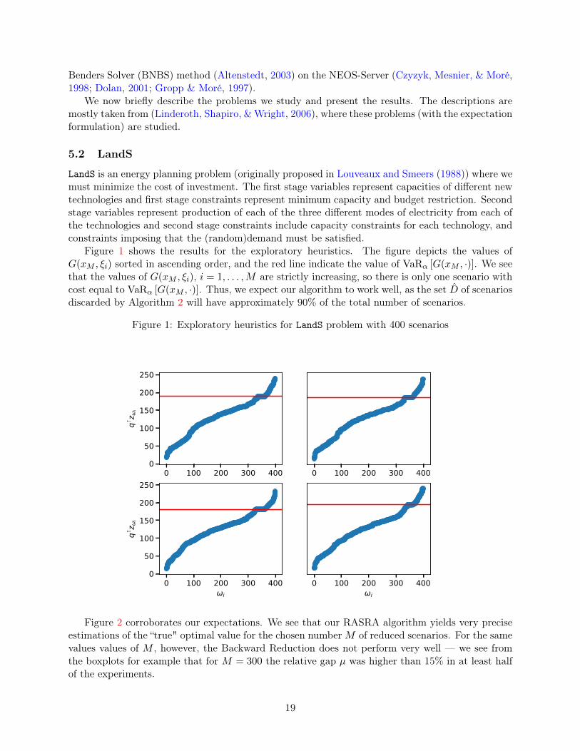
Figure 1 shows the results for the exploratory heuristics. The figure depicts the values ofG(xM , ξi) sorted in ascending order, and the red line indicate the value of VaRα [G(xM , ·)]. We seethat the values of G(xM , ξi), i = 1, . . . ,M are strictly increasing, so there is only one scenario withcost equal to VaRα [G(xM , ·)]. Thus, we expect our algorithm to work well, as the set D of scenariosdiscarded by Algorithm 2 will have approximately 90% of the total number of scenarios.
Figure 1: Exploratory heuristics for LandS problem with 400 scenarios
0 100 200 300 4000
50
100
150
200
250
qz
i
0 100 200 300 400
0 100 200 300 400i
0
50
100
150
200
250
qz
i
0 100 200 300 400i
Figure 2 corroborates our expectations. We see that our RASRA algorithm yields very preciseestimations of the “true" optimal value for the chosen numberM of reduced scenarios. For the samevalues values of M , however, the Backward Reduction does not perform very well — we see fromthe boxplots for example that for M = 300 the relative gap µ was higher than 15% in at least halfof the experiments.
19

Figure 2: Backward Reduction versus RASRA in LandS problem
200 300 400Reduced Cardinality
0.4
0.3
0.2
0.1
0.0V(
P o)
V(P r
)V(
P o)
Dupavcova Technique
200 300 400Reduced Cardinality
Our Technique
5.3 gbd
The gbd problem (proposed originally by G. Dantzig (1963)) considers the allocation of differenttypes of aircraft which need to be assigned to routes in a way that maximizes profit under uncertaindemand . Besides the cost of operating the aircraft, there are costs associated with bumpingpassengers when the demand for seats outstrips the capacity. The first stage variables are thenumber of aircraft of each type allocated to each route and the first-stage constraints boundsnumber available aircraft of each type. The second-stage variables indicate the number of carriedpassengers and the number of bumped passengers on each route and second-stage constraints aredemand balance equations for the routes.
Again, we start with the exploratory heuristics, shown in Figure 3. Here we see that there aremany scenarios with cost equal to VaRα [G(xM , ·)], and in fact there is no scenario with cost strictlybelow that value. Thus, we do not expect our algorithm to perform particularly well in this case.
Figure 4 shows the box-plots for the relative gaps µ. While our method still outperforms theBackward Heuristics, we see that the box-plots for RASRA are farther form zero than in the LandScase.
5.4 gbd-sk3
Problem gbd-sk3 is a modification of the gbd proposed in Cotton and Ntaimo (2015) which changesthe distribution of the underlying random variable. This change in the distribution shows a signifi-cant difference in the graphs depicting the exploratory heuristics. We see a behavior similar to theLandS problem, so we expect RASRA to perform equally well.
Figure 6 again corroborates our expectations. Note however that, while RASRA outperformsthe Backward Reduction method. the latter also performs very well, with largest relative gap beingequal to 0.5% for M = 200.
20

Figure 3: Exploratory heuristics for gbd problem with 400 scenarios
0 100 200 300 400
1750
2000
2250
2500
2750
3000q
zi
0 100 200 300 400
0 100 200 300 400i
1750
2000
2250
2500
2750
3000
qz
i
0 100 200 300 400i
Figure 4: Backward Reduction versus RASRA in gbd problem
200 300 400Reduced Cardinality
0.025
0.020
0.015
0.010
0.005
0.000
V(P o
)V(
P r)
V(P o
)
Backward Reduction
200 300 400Reduced Cardinality
RASRA
6 Conclusions
We have presented a new scenario reduction approach for risk-averse stochastic optimization prob-lems where the objective function is the Conditional Value-at-Risk. Our approach, which relies onthe notion of effective scenarios recently introduced in the literature, makes precise the intuitivenotion that “only the scenarios in the tail matter" and alerts for the case in which many scenarios
21

Figure 5: Exploratory heuristics for gbd-sk3 problem with 400 scenarios
0 100 200 300 400
6000
8000
10000
qz
i
0 100 200 300 400
0 100 200 300 400i
6000
8000
10000
qz
i
0 100 200 300 400i
Figure 6: Backward Reduction versus RASRA in gbd-sk3 problem
200 300 400Reduced Cardinality
0.002
0.001
0.000
0.001
0.002
0.003
0.004
0.005
V(P o
)V(
P r)
V(P o
)
Backward Reduction
200 300 400Reduced Cardinality
RASRA
have the same cost equal to the Value-at-Risk, an issue that appears to have overlooked in theliterature.
Our method combines techniques from three different fronts: the concepts of effective scenarios,classical scenario reduction techniques based on probability metrics, and computational methodsfor facility location problems. While it has been recognized in the literature that some scenario
22
reduction methods are related to facility location problems, it appears that the vast literature (andcomputational methods) on that topic has not been much exploited in the context of scenarioreduction. The numerical results presented in this paper suggest that our approach can be veryuseful for the problems it proposes to solve.
Acknowledgments
This work has been supported by FONDECYT 1171145, Chile.
References
Ahmed, S. (2006). Convexity and decomposition of mean-risk stochastic programs. MathematicalProgramming , 106 (3), 433–446.
Altenstedt, F. (2003). Aspects on asset liability management via stochastic programming. ChalmersUniversity of Technology.
Artzner, P., Delbaen, F., Eber, J.-M., & Heath, D. (1999). Coherent measures of risk. Math Financ,9 , 203–227.
Birge, J. R., & Louveaux, F. (2011). Introduction to stochastic programming. Springer Science &Business Media.
Cotton, T. G., & Ntaimo, L. (2015). Computational study of decomposition algorithms for mean-risk stochastic linear programs. Mathematical Programming Computation, 7 (4), 471–499.
Czyzyk, J., Mesnier, M. P., & Moré, J. J. (1998). The neos server. IEEE Journal on ComputationalScience and Engineering , 5 (3), 68 – 75.
Dantzig, G. (1963). Linear programming and extensions. Princeton, New Jersey: Princeton Uni-versity Press.
Dantzig, G. B. (1955). Linear programming under uncertainty. Management science, 1 (3-4),197–206.
Dolan, E. D. (2001). The neos server 4.0 administrative guide (Technical Memorandum No.ANL/MCS-TM-250). Mathematics and Computer Science Division, Argonne National Labo-ratory.
Dupačová, J., Gröwe-Kuska, N., & Römisch, W. (2003). Scenario reduction in stochastic program-ming. Mathematical programming , 95 (3), 493–511.
Dupačová, J., Consigli, G., & Wallace, S. W. (2000). Scenarios for multistage stochastic programs.Ann Oper Res, 100 , 25–53.
Dupačová, J., Gröwe-Kuska, N., & Römisch, W. (2003). Scenario reduction in stochastic program-ming: An approach using probability metrics. Math Program, 95 , 493–511.
Eichhorn, A., & Römisch, W. (2008). Stability of multistage stochastic programs incorporatingpolyhedral risk measures. Optimization, 57 (2), 295–318.
Espinoza, D., & Moreno, E. (2014). A primal-dual aggregation algorithm for minimizing conditionalvalue-at-risk in linear programs. Computational Optimization and Applications, 59 (3), 617–638.
Fairbrother, J., Turner, A., & Wallace, S. (2015). Scenario generation for stochastic programs withtail risk measures. arXiv preprint arXiv:1511.03074 .
García, S., Labbé, M., & Marín, A. (2011). Solving large p-median problems with a radius formu-lation. INFORMS Journal on Computing , 23 (4), 546–556.
García-Bertrand, R., & Mínguez, R. (2014). Iterative scenario based reduction technique for stochas-tic optimization using conditional value-at-risk. Optimization and Engineering , 15 (2), 355–380.
23

Gropp, W., & Moré, J. J. (1997). Optimization environments and the neos server. In MartinD. Buhman and Arieh Iserles (Ed.), Approximation theory and optimization (pp. 167 – 182).Cambridge University Press.
Guigues, V., Krätschmer, V., & Shapiro, A. (2016). Statistical inference and hypotheses testing ofrisk averse stochastic programs. arXiv preprint arXiv:1603.07384 .
Heitsch, H., & Römisch, W. (2003). Scenario reduction algorithms in stochastic programming.Comput Optim Appl , 24 , 187–206.
Heitsch, H., & Römisch, W. (2009). Scenario tree modeling for multistage stochastic programs.Math Program, 118 , 371–406.
Homem-de-Mello, T., & Bayraksan, G. (2014). Monte Carlo sampling-based methods for stochasticoptimization. Surveys in Operations Research and Management Science, 19 , 56–85.
Hoyland, K., Kaut, M., & Wallace, S. W. (2003). A heuristic for moment-matching scenariogeneration. Comput Optim Appl , 24 , 169–185.
Hoyland, K., & Wallace, S. W. (2001). Generating scenario trees for multistage decision problems.Manage Sci , 47 (2), 295–307.
Linderoth, J., Shapiro, A., & Wright, S. (2006). The empirical behavior of sampling methods forstochastic programming. Annals of Operations Research, 142 (1), 215–241.
Louveaux, F., & Smeers, Y. (1988). Optimal investments for electricity generation: A stochasticmodel and a test problem. In Y. Ermoliev & R. J.-B. Wets (Eds.), Numerical techniques forstochastic optimization problems (pp. 445–452). Berlin: Springer-Verlag.
McKay, M. D., Beckman, R. J., & Conover, W. J. (1979). A comparison of three methods for select-ing values of input variables in the analysis of output from a computer code. Technometrics,21 , 239–245.
Mehrotra, S., & Papp, D. (2014). A cutting surface algorithm for semi-infinite convex programmingwith an application to moment robust optimization. SIAM Journal on Optimization, 24 (4),1670–1697.
Miller, N., & Ruszczynski, A. (2011). Risk-averse two-stage stochastic linear programming: Mod-eling and decomposition. Oper Res, 59 , 125–132.
Noyan, N. (2012). Risk-averse two-stage stochastic programming with an application to disastermanagement. Computers & Operations Research, 39 (3), 541–559.
Pflug, G. C. (2001). Scenario tree generation for multiperiod financial optimization by optimaldiscretization. Mathematical Programming, Series B , 89 (2), 251–271.
Pflug, G. C., & Pichler, A. (2011). Approximations for probability distributions and stochasticoptimization problems. In M. Bertocchi, G. Consigli, & M. A. H. Dempster (Eds.), Stochasticoptimization methods in finance and energy (pp. 343–387). Springer.
Pineda, S., & Conejo, A. (2010). Scenario reduction for risk-averse electricity trading. IET gener-ation, transmission & distribution, 4 (6), 694–705.
Rachev, S. T. (1991). Probability metrics and the stability of stochastic models (Vol. 269). JohnWiley & Son Ltd.
Rahimian, H., Bayraksan, G., & Homem-de Mello, T. (2018). Identifying effective scenariosin distributionally robust stochastic programs with total variation distance. Mathemati-cal Programming . Retrieved from https://doi.org/10.1007/s10107-017-1224-6 doi:10.1007/s10107-017-1224-6
Rockafellar, R. T., & Uryasev, S. P. (2000). Optimization of conditional value-at-risk. J. Risk , 2 ,21–41.
Rockafellar, R. T., & Wets, R. J. (1998). Variational analysis: Grundlehren der mathematischenwissenschaften. Springer Berlin.
24

Römisch, W., & Wets, R.-B. (2007). Stability of ε-approximate solutions to convex stochasticprograms. SIAM Journal on Optimization, 18 (3), 961–979.
Shapiro, A. (2003). Inference of statistical bounds for multistage stochastic programming problems.Math. Meth. Oper. Res., 58 , 57–68.
Shapiro, A., Dentcheva, D., & Ruszczyński, A. (2014). Lectures on stochastic programming :modeling and theory (2nd ed.). SIAM.
Wallace, S. W., & Ziemba, W. T. (2005). Applications of stochastic programming (Vol. 5). Siam.
25