Data-Driven Risk-Averse Stochastic Optimization with

Wasserstein Metric∗

Chaoyue Zhao† and Yongpei Guan‡

†School of Industrial Engineering and Management

Oklahoma State University, Stillwater, OK 74074

‡Department of Industrial and Systems Engineering

University of Florida, Gainesville, FL 32611

Emails: chaoyue.zhao@okstate.edu; guan@ise.ufl.edu

Abstract

The traditional two-stage stochastic programming approach is to minimize the total expected

cost with the assumption that the distribution of the random parameters is known. However, in

most practices, the actual distribution of the random parameters is not known, and instead, only

a series of historical data are available. Thus, the solution obtained from the traditional two-

stage stochastic program can be biased and suboptimal for the true problem, if the estimated

distribution of the random parameters is not accurate, which is usually true when only a limited

amount of historical data are available. In this paper, we propose a data-driven risk-averse

stochastic optimization approach. Based on the observed historical data, we construct the

confidence set of the ambiguous distribution of the random parameters, and develop a risk-

averse stochastic optimization framework to minimize the total expected cost under the worst-

case distribution within the constructed confidence set. We introduce the Wasserstein metric

to construct the confidence set and by using this metric, we can successfully reformulate the

risk-averse two-stage stochastic program to its tractable counterpart. In addition, we derive

the worst-case distribution and develop efficient algorithms to solve the reformulated problem.

Moreover, we perform convergence analysis to show that the risk averseness of the proposed

formulation vanishes as the amount of historical data grows to infinity, and accordingly, the

corresponding optimal objective value converges to that of the traditional risk-neutral two-

stage stochastic program. We further precisely derive the convergence rate, which indicates the

value of data. Finally, the numerical experiments on risk-averse stochastic facility location and

stochastic unit commitment problems verify the effectiveness of our proposed framework.

Key words: stochastic optimization; data-driven decision making; Wasserstein metric

∗The basic idea and main results of this paper are also available in [29] and in the first author’s dissertation [27].

1

1 Introduction

Solving optimization problems under uncertainty has always been challenging for most practitioners.

In an uncertain environment, decision-makers commonly face the following two-stage optimization

problem: minx∈X c>x+Q(x, ξ), where x is the first-stage decision variable and accordingly X ⊆ Rn

is a compact and convex set representing the feasible region for the first-stage decision variable.

The random parameter ξ ∈ Rm represents the uncertainty and the corresponding second-stage cost

Q(x, ξ) = miny(ξ)∈Y

d>y(ξ) : A(ξ)x+By(ξ) ≥ b(ξ), (1)

which is assumed continuous in ξ. To capture the uncertainty of ξ and solve the problems effec-

tively, two branches of optimization under uncertainty approaches, named robust and stochastic

optimization approaches, are studied extensively recently.

For the robust optimization approach, the ambiguity of the random parameters is allowed. This

approach defines an uncertainty set U for the random parameters, e.g., ξ ∈ U , and achieves the

objective of minimizing the total cost under the worst-case realization of ξ in this predefined set

U [2, 5], i.e., minx∈X c>x + maxξ∈U Q(x, ξ). For the cases under the general settings, the robust

optimization model (RP) is intractable. However, for certain special forms of the uncertainty set

U , such as ellipsoidal uncertainty set [3, 11, 13], polyhedral uncertainty set [3], and cardinality

uncertainty set [5], the reformulations of robust optimization are possible to be obtained and

thus the problem can be addressed efficiently. Considering the fact that the robust optimization

approach utilizes limited information (e.g., lower/upper bound of the uncertain parameter plus a

budget constraint) of the random parameters and considers the worst-case cost in the objective,

practitioners are aware of its over-conservatism, although this approach has significant advantages

in terms of providing reliable solutions for most practices.

Stochastic optimization is another effective approach to address uncertainty. The traditional

two-stage stochastic optimization framework can be described as follows (cf. [7] and [21]):

(SP) minx∈X c>x+ EP[Q(x, ξ)],

where the uncertain random variable ξ is defined on a probability space (Ω, σ(Ω),P), in which Ω

2

is the sample space for ξ, σ(Ω) is the σ-algebra of Ω, and P is the associate probability measure.

For this setting, the probability distribution P is given. To solve the problem, the sample average

approximation method [21] is usually applied in which the random parameters are captured by a

number of scenarios sampled from the true distribution. This approach becomes computationally

heavy when the number of scenarios increases.

Considering the disadvantages of robust and stochastic optimization approaches, plus the fact

that the true distribution of the random parameters is usually unknown and hard to predict ac-

curately and the inaccurate estimation of the true distribution may lead to biased solutions and

make the solutions sub-optimal, the distributionally robust optimization approaches are proposed

recently (see, [9], among others) and can be described as follows:

(DR-SP) minx∈X c>x+ maxP∈D

EP[Q(x, ξ)].

Instead of assuming that the distribution of the random parameters is known, this framework allows

distribution ambiguity and introduces a confidence set D to ensure that the true distribution P is

within this set with a certain confidence level based on statistical inference. The objective is to

minimize the total cost under the worst-case distribution in the given confidence set. Moment-based

approaches described below are initially introduced to build the set D [9]:

D1 = P ∈M+ : (EP[ξ]− µ0)>Σ−10 (EP[ξ]− µ0) ≤ γ1, EP[(ξ − µ0)(ξ − µ0)>] γ2Σ0, (2)

where M+ represents the set of all probability distributions, µ0 and Σ0 0 represent the inferred

mean and covariance matrix respectively, and γ1 > 0 and γ2 > 1 are two parameters obtained

from the process of inference (e.g., through sample mean and covariance matrix). In (2), the first

constraint ensures the mean of ξ is in an ellipsoid with center µ0 and size γ1, and the second

constraint ensures the second moment matrix of ξ is in a positive semidefinite cone. The moment-

based approaches have advantages of transforming the original risk-averse stochastic optimization

problem to a tractable conic or semidefinite program. The readers are referred to related pioneer

works, including the special case without considering moment ambiguity, e.g., D01 = P ∈ M+ :

EP[ξ] = µ0,EP[ξξ>] = µ0µ>0 + Σ0, in [12], [14], [8], [23], [30], and [31], among others. For these

3

moment-based approaches, the parameters of γ1 and γ2 can depend on the amount of historical

data available. As the number of historical data increases, the values of γ1 and γ2 decrease and

eventually D1 is constructed with fixed moments, i.e., D1 converges to D01. Note here that although

the confidence set D1 can characterize the properties of the first and second moments of the random

parameters, it cannot guarantee any convergence properties for the unknown distribution to the

true distribution. Even for the case in which there are an infinite amount of historical data, it

is only guaranteed that the first and second moments of the random parameters are estimated

accurately. But there are still infinite distributions, including the true distribution, in D1 with the

same first and second moments.

In this paper, instead of utilizing the moment-based approaches, we propose a “distribution-

based” approach to construct the confidence set for the unknown true distribution. For our ap-

proach, we use the empirical distribution based on the historical data as the reference distribution.

Then, the confidence set D is constructed by utilizing metrics to define the distance between the

reference distribution and the true distribution. The advantage for this approach is that the con-

vergence properties hold. That is, as the number of historical data increases, we can show that

the confidence set D shrinks with the same confidence level guarantee, and accordingly the true

distribution will be “closer” to the reference distribution. For instance, if we let dM(P0, P) be any

metric between a reference distribution P0 and an unknown distribution P and use θ to represent

the corresponding distance, then the confidence set D can be represented as follows:

D = P : dM(P0, P) ≤ θ.

By learning from the historical data, we can build a reference distribution P0 of the uncertain

parameter as well as a confidence set of the true distribution described above, and decisions are

made in consideration of that the true distribution can vary within the confidence set. In particular,

we use the Wasserstein metric to construct the confidence set for general distributions, including

both discrete and continuous distributions. Although significant research progress has been made

for the discrete distribution case (see, e.g., [18] and [16]), the study for the continuous distribution

case is more challenging and is very limited. The recent study on the general φ-divergence [1] can be

utilized for the continuous distribution case by defining the distance between the true density and

4

the reference density, which however could not guarantee the convergence properties. In this paper,

by studying the Wasserstein metric and deriving the corresponding convergence rate, our proposed

approach can fit well in the data-driven risk-averse two-stage stochastic optimization framework.

Our contributions can be summarized as follows:

1. We propose a data-driven risk-averse two-stage stochastic optimization framework to solve

optimization under uncertainty problems by allowing distribution ambiguity. In particular,

we introduce the Wasserstein metric to construct the confidence set and accordingly we can

successfully reformulate the risk-averse stochastic program to its tractable counterpart.

2. Our proposed framework allows the true distribution to be continuous, and closed-form ex-

pressions of the worst-case distribution can be obtained by solving the proposed model.

3. We show the convergence property of the proposed data-driven framework by proving that

as the number of historical data increases, the risk-averse problem converges to the risk-

neutral one, i.e., the traditional stochastic optimization problem. We also provide a tighter

convergence rate, which shows the value of data.

4. The computational experiments on the data-driven risk-averse stochastic facility location and

unit commitment problems numerically show the effectiveness of our proposed approach.

The remainder of this paper is organized as follows. In Section 2, we describe the data-driven

risk-averse stochastic optimization framework, including the introduction of the Wasserstein metric

and the reference distribution and confidence set construction based on the available historical data.

In Section 3, we derive a tractable reformulation of the proposed data-driven risk-averse stochastic

optimization problem, as well as the corresponding worst-case distribution. In Section 4, we show

the convergence property by proving that as the number of historical data increases, the data-driven

risk-averse stochastic optimization problem converges to the traditional risk-neutral one. In Section

5, we propose a solution approach to solve the reformulated problem corresponding to a given finite

set of historical data. In Section 6, we perform numerical studies on stochastic facility location

and unit commitment problems to verify the effectiveness of our solution framework. Finally, in

Section 7, we conclude our study.

5

2 Data-Driven Risk-Averse Stochastic Optimization Framework

In this section, we develop the data-driven risk-averse two-stage stochastic optimization framework,

for which instead of knowing the exact distribution of the random parameters, a series of historical

data are observed. We first introduce the Wasserstein distribution metric. By using this metric,

based on the observed historical data, we then build the reference distribution and the confidence

set for the true probability distribution. Finally, we derive the convergence rate and provide the

formulation framework of the data-driven risk-averse two-stage stochastic optimization problem.

2.1 Wasserstein Metric

The Wasserstein metric is defined as a distance function between two probability distributions on

a given compact supporting space Ω. More specifically, given two probability distributions P and

P on the supporting space Ω, the Wasserstein metric is defined as

dW(P, P) := infπEπ[ρ(X,Y )] : P = L(X), P = L(Y ), (3)

where ρ(X,Y ) is defined as the distance between random variables X and Y , and the infimum is

taken over all joint distributions π with marginals P and P. As indicated in [25], the Wasserstein

metric is indeed a metric since it satisfies the properties of metrics. That is, dW(P, P) = 0 if and

only if P = P, dW(P, P) = dW(P,P) (symmetric property) and dW(P, P) ≤ dW(P,O) + dW(O, P)

for any probability distribution O (triangle equality). In addition, by the Kantorovich-Rubinstein

theorem [15], the Wasserstein metric is equivalent to the Kantorovich metric, which is defined as

dK(P, P) = maxh∈H

∣∣∣∣∫ΩhdP−

∫ΩhdP

∣∣∣∣ ,where H = h : ‖h‖

L≤ 1, and ‖h‖

L:= sup(h(x)− h(y))/ρ(x, y) : x 6= y in Ω. The Wasserstein

metric is commonly applied in many areas. For example, many metrics known in statistics, measure

theory, ergodic theory, functional analysis, etc., are special cases of the Wasserstein/Kantorovich

metric [24]. The Wasserstein/Kantorovich metric also has many applications in transportation the-

ory [19], and some applications in computer science like probabilistic concurrency, image retrieval,

data mining, and bioinformatics, etc [10]. In this study, we use the Wasserstein metric to construct

6

the confidence set for the general probability distribution, including both discrete and continuous

distributions.

2.2 Reference Distribution

After observing a series of historical data, we can have an estimation of the true probability dis-

tribution, which is called reference probability distribution. Intuitively, the more historical data

we have, the more accurate estimation of the true probability distribution we can obtain. Many

significant works have been made to obtain the reference distribution, with both parametric and

nonparametric statistical estimation approaches. For instance, for the parametric approaches, the

true probability distribution is usually assumed following a particular distribution function, e.g.,

normal distribution, and the parameters (e.g., mean and variance) are estimated by learning from

the historical data. On the other hand, the nonparametric estimations (in which the true distri-

bution is not assumed following any specific distribution), such as kernel density estimation, are

also proved to be effective approaches to obtain the reference probability distribution (e.g., [20]

and [17]). In this paper, we utilize a nonparametric estimation approach. More specifically, we use

the empirical distribution to estimate the true probability distribution. The empirical distribution

function is a step function that jumps up by 1/N at each of the N independent and identically-

distributed (i.i.d.) data points. That is, given N i.i.d. historical data samples ξ10 , ξ

20 , · · · , ξN0 , the

empirical distribution is defined as

P0(x) =1

N

N∑i=1

δξi0(x),

where δξi0(x) is one if x ≥ ξi0 and zero elsewhere. Based on the strong law of large numbers, it can

be proved that the reference distribution P0 pointwise converges to the true probability distribution

P almost surely [22]. By Glivenko-Cantelli theorem, this result can be strengthened by proving the

uniform convergence of P to P0 [26].

2.3 Confidence Set Construction

With the previously defined probability metric and reference probability distribution, we can now

construct the confidence set for the true probability distribution P. Intuitively, the more historical

7

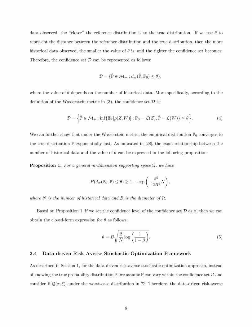
data observed, the “closer” the reference distribution is to the true distribution. If we use θ to

represent the distance between the reference distribution and the true distribution, then the more

historical data observed, the smaller the value of θ is, and the tighter the confidence set becomes.

Therefore, the confidence set D can be represented as follows:

D = P ∈M+ : dW(P,P0) ≤ θ,

where the value of θ depends on the number of historical data. More specifically, according to the

definition of the Wasserstein metric in (3), the confidence set D is:

D =P ∈M+ : inf

πEπ[ρ(Z,W )] : P0 = L(Z), P = L(W ) ≤ θ

. (4)

We can further show that under the Wasserstein metric, the empirical distribution P0 converges to

the true distribution P exponentially fast. As indicated in [28], the exact relationship between the

number of historical data and the value of θ can be expressed in the following proposition:

Proposition 1. For a general m-dimension supporting space Ω, we have

P (dW(P0,P) ≤ θ) ≥ 1− exp

(− θ2

2B2N

),

where N is the number of historical data and B is the diameter of Ω.

Based on Proposition 1, if we set the confidence level of the confidence set D as β, then we can

obtain the closed-form expression for θ as follows:

θ = B

√2

Nlog

(1

1− β

). (5)

2.4 Data-driven Risk-Averse Stochastic Optimization Framework

As described in Section 1, for the data-driven risk-averse stochastic optimization approach, instead

of knowing the true probability distribution P, we assume P can vary within the confidence set D and

consider E[Q(x, ξ)] under the worst-case distribution in D. Therefore, the data-driven risk-averse

8

two-stage stochastic optimization problem can be formulated as follows:

(DD-SP) minx∈X

c>x+ maxP∈D

EP[Q(x, ξ)],

where Q(x, ξ) = miny(ξ)∈Y d>y(ξ) : A(ξ)x+By(ξ) ≥ b(ξ) and P is an arbitrary probability distri-

bution in D. In this case, the proposed approach is more conservative than the traditional stochastic

optimization approach. That is, the proposed approach is risk-averse.

3 Tractable Reformulation and Worst-Case Distribution

In this section, we first derive the reformulation of the worst-case expectation maxP∈D EP[Q(x, ξ)],

and then obtain the reformulation of problem (DD-SP) correspondingly. Following that, we derive

the worst-case distribution corresponding to the Wasserstein metric.

Without loss of generality, we can define the supporting space Ω by assuming that the random

parameter ξ is between a lower bound W− and an upper bound W+. That is,

Ω :=

ξ ∈ Rm : W− ≤ ξ ≤W+

. (6)

Now we can derive the reformulation of the worst-case expectation maxP∈D EP[Q(x, ξ)] in the

following proposition.

Proposition 2. Assuming there are N historical data samples ξ1, ξ2, · · · , ξN which are i.i.d. drawn

from the true continuous distribution P, for any fixed first-stage decision x, we have

maxP∈D

EP[Q(x, ξ)] = minβ≥0

1

N

N∑i=1

maxξ∈ΩQ(x, ξ)− βρ(ξ, ξi)+ θβ

.

Proof. As indicated in Section 2.2, if we have N historical data samples ξ1, ξ2, · · · , ξN , the ref-

erence distribution P0 can be defined as the empirical distribution, i.e., P0 = 1N

∑Ni=1 δξi(x). In

addition, the confidence set D is defined the same way as indicated in (4). Then, we can claim

that, if P ∈ D, then ∀ε ≥ 0, there exists a joint distribution π such that P0 = L(Z), P = L(W ),

and Eπ[ρ(Z,W )] ≤ θ + ε. Based on the definition of Eπ[ρ(Z,W )], we can obtain the following

reformulation of Eπ[ρ(Z,W )] (without loss of generality, we assume the cumulative distribution

9

function for P is absolute continuous):

Eπ[ρ(Z,W )] =

∫z∈Ω

∫ξ∈Ω

f(ξ, z)ρ(ξ, z)dξdz =N∑i=1

∫ξ∈Ω

fW |Z(ξ|ξi)P0(Z = ξi)ρ(ξ, ξi)dξ

=1

N

N∑i=1

∫ξ∈Ω

fW |Z(ξ|ξi)ρ(ξ, ξi)dξ, (7)

where f(ξ, z) is the density function of π, and fW |Z(ξ|ξi) is the conditional density function when

Z = ξi. The equation (7) holds since according to the definition of P0, P0(Z = ξi) = 1/N for

∀i = 1, · · ·N . For notation brevity, we let f i(ξ) = fW |Z(ξ|ξi) and ρi(ξ) = ρ(ξ, ξi). Then the

second-stage problem maxP∈D EP[Q(x,ξ)] of (DD-SP) can be reformulated as:

maxfW(ξ)≥0

∫ξ∈ΩQ(x, ξ)fW(ξ)dξ

s.t. fW(ξ) =1

N

N∑i=1

f i(ξ), (8)∫ξ∈Ω

f i(ξ)dξ = 1, ∀i, (9)

1

N

N∑i=1

∫ξ∈Ω

f i(ξ)ρi(ξ)dξ ≤ θ + ε, (10)

where fW(ξ) is the density function of P. Constraints (8) and (9) are based on the properties of

conditional density function and constraint (10) follows the definition of D and equation (7). Note

here that this reformulation holds for any ε ≥ 0. By substituting constraint (8) into the objective

function, we can obtain its equivalent formulation as follows:

maxf i(ξ)≥01

N

N∑i=1

∫ξ∈ΩQ(x, ξ)f i(ξ)dξ

(P1) s.t.

∫ξ∈Ω

f i(ξ)dξ = 1, ∀i, (11)

1

N

N∑i=1

∫ξ∈Ω

f i(ξ)ρi(ξ)dξ ≤ θ + ε. (12)

Note here that N is a finite number and we can switch the integration and summation in the

objective function. In addition, the above formulation (P1) always has a feasible solution (e.g.,

the reference distribution P0 is obvious a feasible solution for (P1)). Meanwhile, since Q(x, ξ) is

10

assumed bounded above, (P1) is bounded above. Furthermore, since the above problem is a convex

programming, there is no duality gap. Then we can consider its Lagrangian dual problem that can

be written as follows:

L(λi, β) = maxf i(ξ)≥0

1

N

N∑i=1

∫ξ∈Ω

(Q(x, ξ)−Nλi − βρi(ξ))f i(ξ)dξ +N∑i=1

λi + (θ + ε)β,

where λi and β ≥ 0 are dual variables of constraints (11) and (12) respectively. The dual problem

then is

minβ≥0,λi

L(λi, β).

Next, we argue that ∀ξ ∈ Ω, Q(x, ξ)−Nλi−βρi(ξ) ≤ 0. If this argument does not hold, then there

exists a ξ0 such that Q(x, ξ0)−Nλi − βρi(ξ0) > 0. It means there exists a strict positive constant

σ, such that Q(x, ξ0) − Nλi − βρi(ξ0) > σ. Based on the definition of Q(x, ξ), it is continuous

with ξ. Also, the distance function ρi(ξ) is continuous on ξ. Therefore, Q(x, ξ) −Nλi − βρi(ξ) is

continuous with ξ. Thus, if Q(x, ξ0)−Nλi−βρi(ξ0) > σ, there exists a small ball B(ξ0, ε′) ⊆ Ω with

a strictly positive measure, such that Q(x, ξ) −Nλi − βρi(ξ) > σ for ∀ξ ∈ B(ξ0, ε′). Accordingly,

we can let f i(ξ) be arbitrary large when ξ ∈ B(ξ0, ε), then L(λi, β) is unbounded, which leads to

a contradiction to the strong duality corresponding to (P1) bounded above. Hence, the argument

Q(x, ξ)−Nλi − βρi(ξ) ≤ 0 for all ξ ∈ Ω holds. In this case,

maxf i(ξ)≥0

1

N

N∑i=1

∫ξ∈Ω

(Q(x, ξ)−Nλi − βρi(ξ))f i(ξ)dξ +

N∑i=1

λi + (θ + ε)β =

N∑i=1

λi + (θ + ε)β, (13)

with optimal solutions satisfying (Q(x, ξ)−Nλi − βρi(ξ))f i(ξ) = 0, i = 1, · · · , N since f i(ξ) ≥ 0.

Then, the dual formulation is reformulated as:

minβ≥0,λi

N∑i=1

λi + (θ + ε)β

s.t. Q(x, ξ)−Nλi − βρi(ξ) ≤ 0, ∀ξ ∈ Ω,∀i = 1, · · · , N. (14)

From the above formulation, it is easy to observe that the optimal solution λi should satisfy

λi =1

Nmaxξ∈ΩQ(x, ξ)− βρi(ξ), (15)

11

and therefore the worst-case expectation maxP∈D EP[Q(x,ξ)] is equivalent to

minβ≥0

1

N

N∑i=1

maxξ∈ΩQ(x, ξ)− βρi(ξ)+ (θ + ε)β

. (16)

Note here that reformulation (16) holds for ∀ε ≥ 0 and is continuous on ε. Thus, reformulation (16)

holds for ε = 0, which immediately leads to the following reformulation of maxP∈D EP[Q(x, ξ)]:

maxP∈D

EP[Q(x, ξ)] = minβ≥0

1

N

N∑i=1

maxξ∈ΩQ(x, ξ)− βρi(ξ)+ θβ

.

Note here that the reformulation of maxP∈D EP[Q(x,ξ)] depends on θ. By defining

g(θ) = minβ≥0

1

N

N∑i=1

maxξ∈ΩQ(x, ξ)− βρi(ξ)+ θβ

,

we have the following proposition:

Proposition 3. The function g(θ) is monotone increasing in θ. In addition, g(0) = EP0 [Q(x,ξ)]

and limθ→∞ g(θ) = maxξ∈ΩQ(x, ξ).

Proof. The monotone property is obvious, since it can be easily observed that as θ decreases, the

confidence set D shrinks and the worst-case expected value maxP∈D EP[Q(x, ξ)] decreases. There-

fore, the reformulation g(θ) = maxP∈D EP[Q(x, ξ)] is monotone in θ.

When θ = 0, we have dW(P0, P) = 0. According to the properties of metrics, we have P = P0.

That means the confidence set D is a singleton, only containing P0. Therefore, we have g(0) =

EP0 [Q(x, ξ)].

When θ →∞, it is clear to observe that in the optimal solution we have β = 0 since ρi(ξ) <∞

following the assumption that Ω is compact. Then we have

minβ≥0

1

N

N∑i=1

maxξ∈ΩQ(x, ξ)− βρi(ξ)+ θβ

=

1

N

N∑i=1

maxξ∈ΩQ(x, ξ) = max

ξ∈ΩQ(x, ξ),

which indicates that limθ→∞ g(θ) = maxξ∈ΩQ(x, ξ). Thus, the claim holds.

12

From Proposition 3 we can observe that, the data-driven risk-averse stochastic optimization

is less conservative than the traditional robust optimization and more robust than the traditional

stochastic optimization.

Now, we analyze the formulation of the worst-case distribution. We have the following propo-

sition.

Proposition 4. The worst-case distribution for maxP∈D EP[Q(x,ξ)] is

P∗(ξ) =1

N

N∑i=1

δξi(ξ),

where δξi(ξ) is one if ξ ≥ ξi and zero elsewhere, and ξi is the optimal solution of maxξ∈ΩQ(x, ξ)−

βρi(ξ).

Proof. Based on (13), we have

maxf i(ξ)≥0

1

N

N∑i=1

∫ξ∈Ω

(Q(x, ξ)−Nλi − βρi(ξ))f i(ξ)dξ = 0.

Therefore, any distribution (corresponding to f i(ξ)) satisfying the above formulation is a worst-case

distribution.

As indicated in (14), we have Q(x, ξ)−Nλi − βρi(ξ) ≤ 0, for ∀ξ ∈ Ω, ∀i. Therefore,

(Q(x, ξ)−Nλi − βρi(ξ))f i(ξ) = 0, ∀ξ ∈ Ω.

Since f i(ξ) ≥ 0, f i(ξ) can be non-zero only when Q(x, ξ) − Nλi − βρi(ξ) = 0, which means

λi = (Q(x, ξ) − βρi(ξ))/N . Meanwhile, as indicated in (15), we have λi = (Q(x, ξ) − βρi(ξ))/N

only when ξ is the optimal solution of maxξ∈ΩQ(x, ξ) − βρi(ξ). Therefore, there exists at least

one distribution function (indicated as Pi(ξ)) of f i(ξ) described as follows:

Pi(ξ) = δξi(ξ),

where ξi is an optimal solution of maxξ∈ΩQ(x, ξ)−βρi(ξ). Accordingly, following (8), there exists

13

at least one worst-case distribution P∗ that satisfies

P∗(ξ) =1

N

N∑i=1

Pi(ξ) =1

N

N∑i=1

δξi(ξ).

Therefore, we have Proposition 4 holds.

Based on Propositions 2 and 4, we can easily derive the following theorem.

Theorem 1. The problem (DD-SP) is equivalent to the following two-stage robust optimization

problem:

(RDD-SP) minx∈X,β≥0

c>x+ θβ +1

N

N∑i=1

maxξ∈Ω

Q(x, ξ)− βρi(ξ)

, (17)

with the worst-case distribution

P∗(ξ) =1

N

N∑i=1

δξi(ξ),

where ξi is the optimal solution of maxξ∈ΩQ(x, ξ)− βρi(ξ).

4 Convergence Analysis

In this section, we examine the convergence properties of the (DD-SP) to (SP) as the amount of

historical data increases. We demonstrate that as the confidence set D shrinks with more historical

data observed, the risk-averse problem (DD-SP) converges to the risk-neutral one (SP). We first

analyze the convergence property of the second-stage objective value, which can be shown as follows:

Proposition 5. Corresponding to each predefined confidence level β, as the amount of historical

data N → ∞, we have the distance value θ → 0 and the corresponding risk-averse second-stage

objective value limθ→0 maxP∈D EP[Q(x, ξ)] = EP[Q(x, ξ)].

Proof. First, following (5), it is obvious that θ → 0 as N →∞. Meanwhile, following Proposition

2, we have

maxP∈D

EP[Q(x, ξ)] = minβ≥0

θβ +

1

N

N∑i=1

maxξ∈ΩQ(x, ξ)− βρi(ξ)

.

14

Therefore, in the following part, we only need to prove

limN→∞

minβ≥0

θβ +

1

N

N∑i=1

maxξ∈ΩQ(x, ξ)− βρi(ξ)

≤ EP[Q(x, ξ)], (18)

and

limθ→0

maxP∈D

EP[Q(x, ξ)] ≥ EP[Q(x, ξ)]. (19)

Note here that (19) is obvious. We only need to prove (18).

Following our assumptions, we have that Ω is compact and Q(x, ξ) is continuous on ξ. Then,

there exists a constant number M > 0 such that for any given x,

−M ≤ Q(x, ξ) ≤M, ∀ξ ∈ Ω. (20)

In addition, we have

0 ≤ ρ(ξ, z) ≤ B, ∀ξ, z ∈ Ω, (21)

where B is the diameter of Ω. Therefore, for any β ≥ 0, based on (20) and (21), we have

maxξ∈ΩQ(x, ξ)− βρ(ξ, z) ≤ max

ξ∈ΩQ(x, ξ) ≤M,

and

maxξ∈ΩQ(x, ξ)− βρ(ξ, z) ≥ max

ξ∈ΩQ(x, ξ)− βB ≥ −M − βB,

which means maxξ∈ΩQ(x, ξ)− βρ(ξ, z) is bounded for ∀z ∈ Ω. Therefore, we have

limN→∞

θβ +

1

N

N∑i=1

maxξ∈ΩQ(x, ξ)− βρ(ξ, zi)

= limN→∞

θβ + EP0 max

ξ∈ΩQ(x, ξ)− βρ(ξ, z)

= lim

N→∞θβ + EP max

ξ∈ΩQ(x, ξ)− βρ(ξ, z)

= EP[maxξ∈ΩQ(x, ξ)− βρ(ξ, z)], (22)

where the first equality holds following the definition of P0, the second equality holds following

the Helly-Bray Theorem [6], because P0 converges in probability to P as N → ∞ (as indicated in

15

Proposition 1) and maxξ∈ΩQ(x,ξ)− βρ(ξ, z) is bounded for ∀z ∈ Ω, and the third equality holds

because θ → 0 as N →∞ following (5).

Now we show that for a given first-stage solution x and any true distribution P, we have the

following claim holds:

minβ≥0

EP[maxξ∈ΩQ(x, ξ)− βρ(ξ, z)] = EP[Q(x, z)]. (23)

To prove (23), we first denote ξ∗(z) as the optimal solution to maxξ∈ΩQ(x, ξ) − βρ(ξ, z) corre-

sponding to a given z. Accordingly, we can write

EP[maxξ∈ΩQ(x, ξ)− βρ(ξ, z)] = EP[Q(x, ξ∗(z))]− βEP[ρ(ξ∗(z), z)].

Considering the assumption made in (20), we have

EP[Q(x, ξ∗(z))]− βEP[ρ(ξ∗(z), z)] ≤M − βEP[ρ(ξ∗(z), z)].

Now we can argue that EP[ρ(ξ∗(z), z)] = 0. If not, then EP[ρ(ξ∗(z), z)] > 0 since ρ(ξ∗(z), z) is

nonnegative. Accordingly, we have

EP[Q(x,ξ∗(z))]− βEP[ρ(ξ∗(z), z)] ≤M − βEP[ρ(ξ∗(z), z)]→ −∞ by letting β →∞,

which contradicts the fact that minβ≥0 EP[maxξ∈ΩQ(x,ξ) − βρ(ξ, z)] is bounded. Therefore,

EP[ρ(ξ∗(z), z)] = 0. Furthermore, since for any z, ρ(ξ∗(z), z) ≥ 0, we have ρ(ξ∗(z), z) = 0 holds

for any z ∈ Ω. It means ξ∗(z) = z, ∀z ∈ Ω. In this case,

minβ≥0

EP[maxξ∈ΩQ(x, ξ)− βρ(ξ, z)]

= minβ≥0

EP[Q(x, ξ∗(z))− βρ(ξ∗(z), z)]

= minβ≥0

EP[Q(x, z)− βρ(z, z)] = EP[Q(x, z)].

Thus, (23) holds. Therefore, we have

16

limN→∞

minβ≥0

θβ +

1

N

N∑i=1

maxξ∈ΩQ(x, ξ)− βρ(ξ, zi)

≤ minβ≥0

limN→∞

θβ +

1

N

N∑i=1

maxξ∈ΩQ(x, ξ)− βρ(ξ, zi)

= min

β≥0EP[max

ξ∈ΩQ(x, ξ)− βρ(ξ, z) = EP[Q(x, ξ)],

where the first equation holds following (22) and the second equation holds following (23). There-

fore, the claim (18) is proved and accordingly the overall conclusion holds.

Now we prove that the objective value of (DD-SP) converges to that of (SP) as the amount of

historical data samples increases to infinity.

Theorem 2. Corresponding to each predefined confidence level β, as the amount of historical

data increases to infinity, the optimal objective value of the data-driven risk-averse stochastic opti-

mization problem converges to that of the traditional two-stage risk-neutral stochastic optimization

problem.

Proof. First, notice that N → ∞ is equivalent to θ → 0 following (5). We only need to prove

limθ→0 ψ(θ) = ψ(0), where ψ(θ) represents the optimal objective value of (DD-SP) with the distance

value θ and ψ(0) represents the optimal objective value of (SP). Meanwhile, for the convenience of

analysis, corresponding to each given first-stage solution x for (DD-SP) with the distance value θ,

we denote Vθ(x) as its corresponding objective value and V0(x) as the objective value of (SP).

Now consider the (DD-SP) problem with the distance value θ and the first-stage solution fixed

as the optimal first-stage solution to (SP) (denoted as x∗). According to Proposition 5, for any

arbitrary small positive number ε, there exists a ∆θ > 0 such that

|Vθ(x∗)− V0(x∗)| ≤ ε, ∀θ ≤ ∆θ.

Then, for any θ ≤ ∆θ, by denoting the optimal solution to (DD-SP) as x∗θ, we have

|ψ(θ)− ψ(0)| = ψ(θ)− ψ(0) = Vθ(x∗θ)− V0(x∗) ≤ Vθ(x∗)− V0(x∗) ≤ |Vθ(x∗)− V0(x∗)| ≤ ε,

17

where the first inequality follows from the fact that x∗θ is the optimal solution to (DD-SP) with

the distance value θ and x∗ is a feasible solution to this same problem. Therefore, the claim is

proved.

5 Solution Approaches

In this section, we discuss a solution approach to solve the data-driven risk-averse stochastic op-

timization problem, i.e., formulation (RDD-SP) as shown in (17), when a finite set of historical

data is given. We develop a Benders’ decomposition algorithm to solve the problem. We first take

the dual of the formulation for the second-stage cost (i.e., Q(x, ξ)) (1) and combine it with the

second-stage problem in (17) to obtain the following subproblem (denoted as SUB) corresponding

to each sample ξj , j = 1, · · · , N :

φj(x) = maxξ∈Ω,λ

(b(ξ)−A(ξ)x)>λ− βρj(ξ)

(SUB) s.t. B>λ ≤ d,

λ ≥ 0,

where λ is the dual variable. Now letting ψj represent the optimal objective value of the subproblem

(SUB) with respect to sample ξj , we can obtain the following master problem:

minx∈X,β≥0 c>x+ θβ +1

N

N∑j=1

ψj

s.t. Feasibility cuts,

Optimality cuts.

The above problem can be solved by adding feasibility and optimality cuts iteratively. Note here

that in the subproblem (SUB), we have a nonlinear term (b(ξ)−A(ξ)x)>λ. In the following part,

we propose two separation approaches to address the nonlinear term.

18

5.1 Exact Separation Approach

There exist exact separation approaches for problem settings in which the supporting space Ω of

the random parameters is defined in (6), the distance function ρ(., .) is defined as the L1-norm, i.e,

ρ(ξ, ξj) =∑m

i=1 |ξi− ξji | for each j = 1, · · ·N (similar results hold for the L∞-norm case), and A(ξ)

and b(ξ) are assumed affinely dependent on ξ, i.e., A(ξ) = A0+∑m

i=1Aiξi, and b(ξ) = b0+∑m

i=1 biξi,

where A0 and b0 are the deterministic parts of A(ξ) and b(ξ) and ξi is the ith component of vector

ξ. Note here that the right-hand-side uncertainty case (i.e., Ax + By ≥ ξ) is a special case of

this problem setting by letting A0 = A, Ai be a zero matrix, b0 = 0, and bi = ei (i.e., the unit

vector with the ith component to be 1). Then, corresponding to each sample ξj , j = 1, · · · , N , the

objective function of (SUB) can be reformulated as

φj(x) = maxξ∈Ω,λ

(b0 −A0x)>λ+m∑i=1

(bi −Aix)>λξi − βm∑i=1

|ξi − ξji |.

Now we derive the optimality conditions for ξ. It can be observed that the optimal solution ξ∗ to

(SUB) should satisfy the following proposition.

Lemma 1. For the subproblem (SUB) corresponding to each historical sample ξj, there exists an

optimal solution (ξ∗, λ∗) such that ξ∗i = W−i , ξ∗i = W+i , or ξ∗i = ξji for each i = 1, 2, · · · ,m.

Proof. For a fixed solution λ∗, obtaining an optimal solution ξ to the problem (SUB) is equivalent

to obtaining an optimal solution to maxξ∈Ω∑m

i=1(bi − Aix)>λ∗ξi − β∑m

i=1 |ξi − ξji |, so it can be

easily observed that at least one optimal solution ξ∗ to the subproblem (SUB) satisfies ξ∗i = W−i ,

ξ∗i = W+i , or ξ∗i = ξji , for each i = 1, 2, · · · ,m.

We let binary variables z+i and z−i indicate the case in which ξ∗i achieves its upper bound and

lower bound respectively, i.e., z+i = 1 ⇔ ξ∗i = W+

i and z−i = 1 ⇔ ξ∗i = W−i . Then, based on

Lemma 1, there exists an optimal solution ξ∗ of (SUB) satisfying the following constraints:

ξi = (W+i − ξ

ji )z

+i + (W−i − ξ

ji )z−i + ξji , ∀i = 1, · · · ,m, (24)

z+i + z−i ≤ 1, z+

i , z−i ∈ 0, 1, ∀i = 1, · · · ,m, (25)

which indicate that for each i = 1, · · · ,m, the ith component of optimal solution ξ∗ can achieve

19

its lower bound W−i (z+i = 0, z−i = 1), upper bound W+

i (z+i = 1, z−i = 0), or the sample value ξji

(z+i = z−i = 0). By letting σi = (bi − Aix)>λ, with constraints (24) and (25), we can linearize the

bilinear term∑m

i=1(bi −Aix)>λξi as follows:

∑mi=1(bi −Aix)>λξi =

m∑i=1

ξiσi =m∑i=1

((W+

i − ξji )z

+i + (W−i − ξ

ji )z−i + ξji

)σi

=m∑i=1

((W+

i − ξji )z

+i σi + (W−i − ξ

ji )z−i σi + ξjiσi

)=

m∑i=1

((W+

i − ξji )σ

+i + (W−i − ξ

ji )σ−i + ξjiσi

)(26)

s.t. σi = (bi −Aix)>λ, ∀i = 1, 2, · · · ,m (27)

σ+i ≤Mz+

i , ∀i = 1, 2, · · · ,m (28)

σ+i ≤ σi +M(1− z+

i ), ∀i = 1, 2, · · · ,m (29)

σ−i ≥ −Mz−i , ∀i = 1, 2, · · · ,m (30)

σ−i ≥ σi −M(1− z−i ), ∀i = 1, 2, · · · ,m (31)

z+i + z−i ≤ 1, ∀i = 1, 2, · · · ,m (32)

z+i , z

−i ∈ 0, 1, ∀i = 1, 2, · · · ,m. (33)

That is, we can replace the bilinear term∑m

i=1(bi−Aix)>λξi with (26) and add constraints (27)-(33)

to the subproblem (SUB).

With the reformulation of the bilinear term∑m

i=1(bi − Aix)>λξi, we can now derive Benders’

feasibility and optimality cuts corresponding to each sample ξj , j = 1, . . . , N .

Corresponding to each particular sample ξj , the feasibility check problem can be described as

follows:

$j(x) = maxz+,z−,σ+,σ−,σ,λ

(b0 −A0x)>λ+ (W+ − ξj)>σ+ + (W− − ξj)>σ− + (ξj)>σ

−βρ((W+ − ξj)>z+ + (W− − ξj)>z− + ξj , ξj)

s.t. B>λ ≤ d,

Constraints (27) to (32) with respect to z+, z−, σ+, σ−, σ, and λ,

λ ∈ [0, 1] and z+, z− ∈ 0, 1.

20

For a given first-stage solution x0, if $j(x0) = 0, then x0 is a feasible solution to (SUB).

Otherwise, if $j(x0) > 0, we can generate a corresponding feasibility cut $j(x) ≤ 0 to the master

problem.

For the optimality cuts, after solving the master problem and obtaining the optimal solutions x0

and ψj0, we substitute x0 into (SUB) and get φj(x0). If φj(x0) > ψj0, we can generate an optimality

cut φj(x) ≤ ψj to the master problem.

5.2 Bilinear Separation Approach

In this section, we discuss the bilinear heuristic separation approach to generate Benders’ cuts.

We employ the similar assumptions as the ones described in the exact separation approach, except

allowing the distance function ρ(., .) to be more general. The feasibility check problem corresponding

to each particular sample ξj is shown as follows (denoted as FEA):

θj(x) = maxξ∈Ω,λ

(b0 −A0x)>λ+

m∑i=1

(bi −Aix)>λξi − βρj(ξ) (34)

(FEA) s.t. B>λ ≤ d,

λ ∈ [0, 1].

Similarly, we have the bilinear term∑m

i=1(bi−Aix)>λξi in the objective function of problem (FEA).

We use the alternative bilinear separation approach to solve (FEA). First, we initiate the value of ξ

as one of the extreme points of Ω. Next, with the fixed ξ, we solve (FEA) to obtain the corresponding

optimal objective value θj(x) (denoted as θj1(x, ξ)) and optimal solution λ∗. Then, by fixing λ = λ∗

and maximizing the objective function (34) with respect to ξ ∈ Ω, we can obtain the corresponding

optimal objective value (denoted as θj2(x, λ)) and optimal solution ξ∗. If θj2(x, λ) > θj1(x, ξ), we let

ξ = ξ∗ and process it iteratively. Otherwise, we check whether θj1(x, ξ) = 0. If so, we can terminate

the feasibility check (FEA); if not, add the feasibility cut θj1(x, ξ) ≤ 0 to the master problem.

We can also use the bilinear heuristic approach to generate the Benders’ optimality cuts. Sim-

ilarly, for each j = 1, · · · , N , we initiate the value of ξ as one extreme point of Ω, and solve the

corresponding subproblem (SUB) to obtain the optimal objective value (denoted as φj1(x, ξ)) and

optimal solution λ∗. Then, by fixing λ = λ∗, we solve (SUB) and obtain the optimal objective

21

value (denoted as φj2(x, λ)) and the corresponding optimal solution ξ∗ of the following problem

φj2(x, λ) = maxξ∈Ω

m∑i=1

(bi −Aix)>λξi − βρj(ξ) + (b0 −A0x)>λ.

If φj2(x, λ) > φj1(x, ξ), we let ξ = ξ∗ and process it iteratively until φj2(x, λ) ≤ φj1(x, ξ). Then we

check whether φj1(x, λ) > ψj . If so, we generate the corresponding optimality cut φj1(x, λ) ≤ ψj to

the master problem.

6 Numerical Studies

In this section, we conduct computational experiments to show the effectiveness of the proposed

data-driven risk-averse stochastic optimization model with Wasserstein metric. We test the system

performance through two instances: Risk-Averse Stochastic Facility Location Problem and Risk-

Averse Stochastic Unit Commitment Problem. In our experiments, we use the L1-norm as described

in Section 5.1 to serve as the distance measure. In addition, we set the feasibility tolerance gap to

be 10−6 and the optimality tolerance gap to be 10−4. The mixed-integer-programming tolerance

gap for the master problem is set the same as the CPLEX default gap. We use C++ with CPLEX

12.1 to implement the proposed formulations and algorithms. All experiments are executed on a

computer workstation with 4 Intel Cores and 8GB RAM.

6.1 Risk-Averse Stochastic Facility Location Problem

We consider a traditional facility location problem in which there are M facility locations and

N demand sites. We let binary variable yi represent whether facility i is open (yi = 1) or not

(yi = 0) and continuous variable xij represent the amount of products to be shipped from facility

i to demand site j. For the problem parameters, we assume that the fixed cost to open facility

i is Fi and the capacity for facility i is Ci. We let the transportation cost for shipping one unit

product from facility i to demand site j be Tij . The demand for each site is uncertain (denoted as

dj(ξ)). Based on this setting, the corresponding data-driven risk-averse two-stage stochastic facility

22

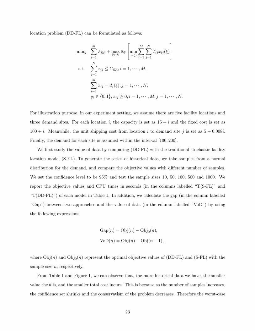
location problem (DD-FL) can be formulated as follows:

miny

M∑i=1

Fiyi + maxP∈D

EP

minx(ξ)

M∑i=1

N∑j=1

Tijxij(ξ)

s.t.

N∑j=1

xij ≤ Ciyi, i = 1, · · · ,M,

M∑i=1

xij = dj(ξ), j = 1, · · · , N,

yi ∈ 0, 1, xij ≥ 0, i = 1, · · · ,M, j = 1, · · · , N.

For illustration purpose, in our experiment setting, we assume there are five facility locations and

three demand sites. For each location i, the capacity is set as 15 + i and the fixed cost is set as

100 + i. Meanwhile, the unit shipping cost from location i to demand site j is set as 5 + 0.008i.

Finally, the demand for each site is assumed within the interval [100, 200].

We first study the value of data by comparing (DD-FL) with the traditional stochastic facility

location model (S-FL). To generate the series of historical data, we take samples from a normal

distribution for the demand, and compare the objective values with different number of samples.

We set the confidence level to be 95% and test the sample sizes 10, 50, 100, 500 and 1000. We

report the objective values and CPU times in seconds (in the columns labelled “T(S-FL)” and

“T(DD-FL)”) of each model in Table 1. In addition, we calculate the gap (in the column labelled

“Gap”) between two approaches and the value of data (in the column labelled “VoD”) by using

the following expressions:

Gap(n) = Obj(n)−Obj0(n),

VoD(n) = Obj(n)−Obj(n− 1),

where Obj(n) and Obj0(n) represent the optimal objective values of (DD-FL) and (S-FL) with the

sample size n, respectively.

From Table 1 and Figure 1, we can observe that, the more historical data we have, the smaller

value the θ is, and the smaller total cost incurs. This is because as the number of samples increases,

the confidence set shrinks and the conservatism of the problem decreases. Therefore the worst-case

23

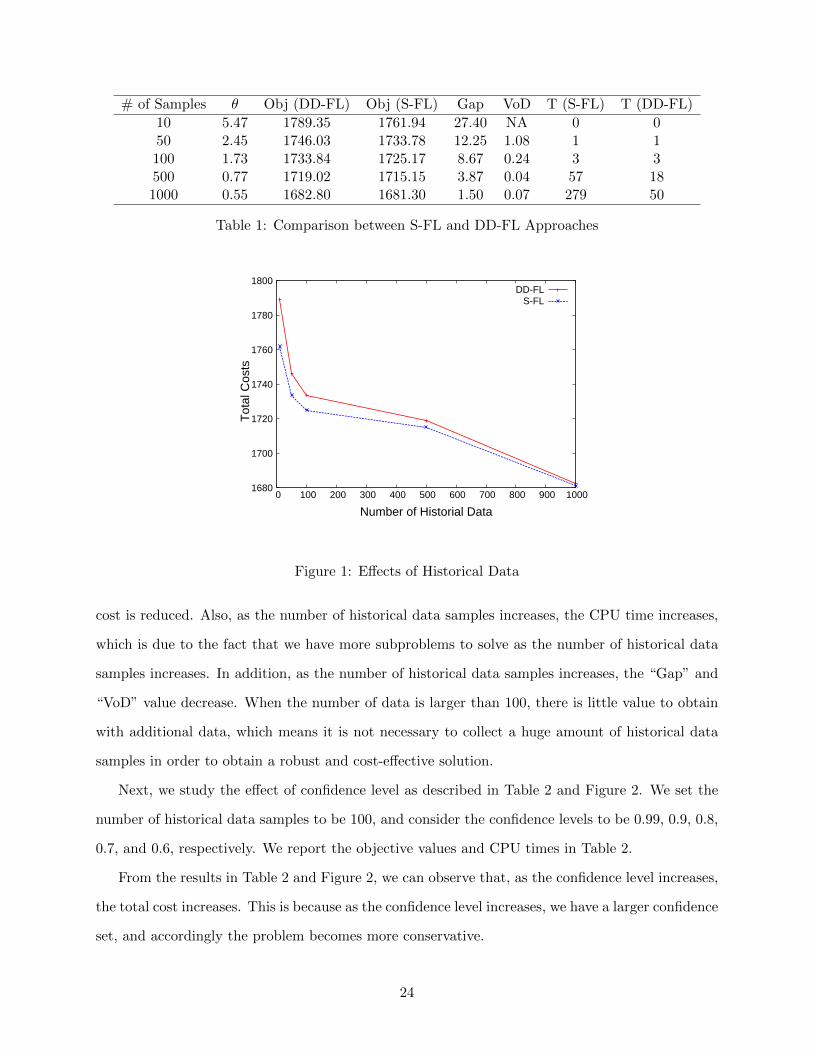
# of Samples θ Obj (DD-FL) Obj (S-FL) Gap VoD T (S-FL) T (DD-FL)

10 5.47 1789.35 1761.94 27.40 NA 0 050 2.45 1746.03 1733.78 12.25 1.08 1 1100 1.73 1733.84 1725.17 8.67 0.24 3 3500 0.77 1719.02 1715.15 3.87 0.04 57 181000 0.55 1682.80 1681.30 1.50 0.07 279 50

Table 1: Comparison between S-FL and DD-FL Approaches

1680

1700

1720

1740

1760

1780

1800

0 100 200 300 400 500 600 700 800 900 1000

Tot

al C

osts

Number of Historial Data

DD-FLS-FL

Figure 1: Effects of Historical Data

cost is reduced. Also, as the number of historical data samples increases, the CPU time increases,

which is due to the fact that we have more subproblems to solve as the number of historical data

samples increases. In addition, as the number of historical data samples increases, the “Gap” and

“VoD” value decrease. When the number of data is larger than 100, there is little value to obtain

with additional data, which means it is not necessary to collect a huge amount of historical data

samples in order to obtain a robust and cost-effective solution.

Next, we study the effect of confidence level as described in Table 2 and Figure 2. We set the

number of historical data samples to be 100, and consider the confidence levels to be 0.99, 0.9, 0.8,

0.7, and 0.6, respectively. We report the objective values and CPU times in Table 2.

From the results in Table 2 and Figure 2, we can observe that, as the confidence level increases,

the total cost increases. This is because as the confidence level increases, we have a larger confidence

set, and accordingly the problem becomes more conservative.

24

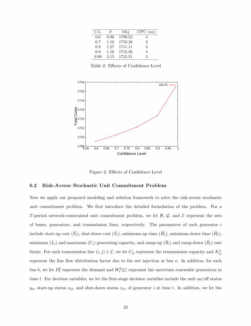
C.L. θ Obj CPU (sec)0.6 0.96 1709.55 40.7 1.10 1710.26 30.8 1.27 1711.11 30.9 1.16 1712.36 40.99 2.15 1715.51 3

Table 2: Effects of Confidence Level

1709

1710

1711

1712

1713

1714

1715

1716

0.55 0.6 0.65 0.7 0.75 0.8 0.85 0.9 0.95 1

Tot

al C

osts

Confidence Level

DD-FL

Figure 2: Effects of Confidence Level

6.2 Risk-Averse Stochastic Unit Commitment Problem

Now we apply our proposed modeling and solution framework to solve the risk-averse stochastic

unit commitment problem. We first introduce the detailed formulation of the problem. For a

T -period network-constrained unit commitment problem, we let B, G, and E represent the sets

of buses, generators, and transmission lines, respectively. The parameters of each generator i

include start-up cost (Si), shut-down cost (Si), minimum-up time (Hi), minimum-down time (Hi),

minimum (Li) and maximum (Ui) generating capacity, and ramp-up (Ri) and ramp-down (Ri) rate

limits. For each transmission line (i, j) ∈ E , we let Cij represent the transmission capacity and Knij

represent the line flow distribution factor due to the net injection at bus n. In addition, for each

bus b, we let Dbt represent the demand and W b

t (ξ) represent the uncertain renewable generation in

time t. For decision variables, we let the first-stage decision variables include the unit on/off status

yit, start-up status uit, and shut-down status vit, of generator i at time t. In addition, we let the

25

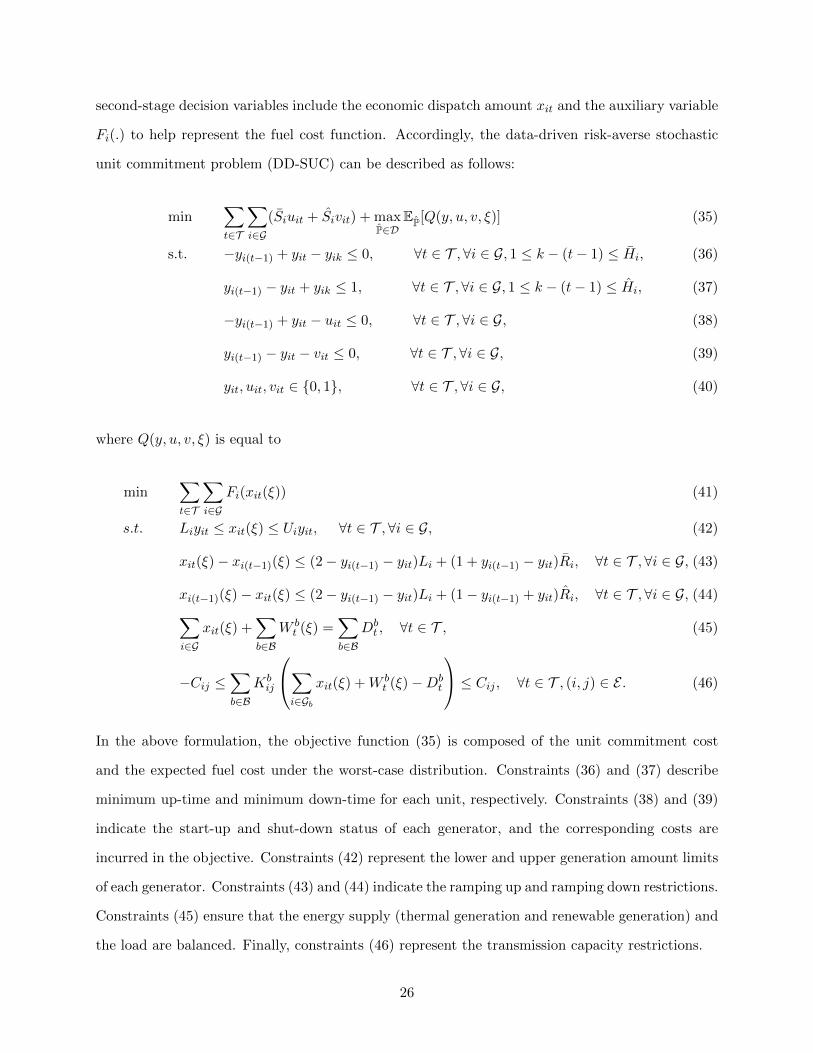
second-stage decision variables include the economic dispatch amount xit and the auxiliary variable

Fi(.) to help represent the fuel cost function. Accordingly, the data-driven risk-averse stochastic

unit commitment problem (DD-SUC) can be described as follows:

min∑t∈T

∑i∈G

(Siuit + Sivit) + maxP∈D

EP[Q(y, u, v, ξ)] (35)

s.t. −yi(t−1) + yit − yik ≤ 0, ∀t ∈ T , ∀i ∈ G, 1 ≤ k − (t− 1) ≤ Hi, (36)

yi(t−1) − yit + yik ≤ 1, ∀t ∈ T ,∀i ∈ G, 1 ≤ k − (t− 1) ≤ Hi, (37)

−yi(t−1) + yit − uit ≤ 0, ∀t ∈ T , ∀i ∈ G, (38)

yi(t−1) − yit − vit ≤ 0, ∀t ∈ T ,∀i ∈ G, (39)

yit, uit, vit ∈ 0, 1, ∀t ∈ T ,∀i ∈ G, (40)

where Q(y, u, v, ξ) is equal to

min∑t∈T

∑i∈G

Fi(xit(ξ)) (41)

s.t. Liyit ≤ xit(ξ) ≤ Uiyit, ∀t ∈ T , ∀i ∈ G, (42)

xit(ξ)− xi(t−1)(ξ) ≤ (2− yi(t−1) − yit)Li + (1 + yi(t−1) − yit)Ri, ∀t ∈ T ,∀i ∈ G, (43)

xi(t−1)(ξ)− xit(ξ) ≤ (2− yi(t−1) − yit)Li + (1− yi(t−1) + yit)Ri, ∀t ∈ T ,∀i ∈ G, (44)∑i∈G

xit(ξ) +∑b∈B

W bt (ξ) =

∑b∈B

Dbt , ∀t ∈ T , (45)

−Cij ≤∑b∈B

Kbij

∑i∈Gb

xit(ξ) +W bt (ξ)−Db

t

≤ Cij , ∀t ∈ T , (i, j) ∈ E . (46)

In the above formulation, the objective function (35) is composed of the unit commitment cost

and the expected fuel cost under the worst-case distribution. Constraints (36) and (37) describe

minimum up-time and minimum down-time for each unit, respectively. Constraints (38) and (39)

indicate the start-up and shut-down status of each generator, and the corresponding costs are

incurred in the objective. Constraints (42) represent the lower and upper generation amount limits

of each generator. Constraints (43) and (44) indicate the ramping up and ramping down restrictions.

Constraints (45) ensure that the energy supply (thermal generation and renewable generation) and

the load are balanced. Finally, constraints (46) represent the transmission capacity restrictions.

26

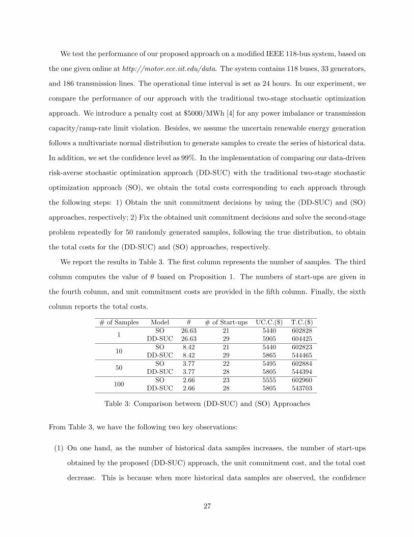
We test the performance of our proposed approach on a modified IEEE 118-bus system, based on

the one given online at http://motor.ece.iit.edu/data. The system contains 118 buses, 33 generators,

and 186 transmission lines. The operational time interval is set as 24 hours. In our experiment, we

compare the performance of our approach with the traditional two-stage stochastic optimization

approach. We introduce a penalty cost at $5000/MWh [4] for any power imbalance or transmission

capacity/ramp-rate limit violation. Besides, we assume the uncertain renewable energy generation

follows a multivariate normal distribution to generate samples to create the series of historical data.

In addition, we set the confidence level as 99%. In the implementation of comparing our data-driven

risk-averse stochastic optimization approach (DD-SUC) with the traditional two-stage stochastic

optimization approach (SO), we obtain the total costs corresponding to each approach through

the following steps: 1) Obtain the unit commitment decisions by using the (DD-SUC) and (SO)

approaches, respectively; 2) Fix the obtained unit commitment decisions and solve the second-stage

problem repeatedly for 50 randomly generated samples, following the true distribution, to obtain

the total costs for the (DD-SUC) and (SO) approaches, respectively.

We report the results in Table 3. The first column represents the number of samples. The third

column computes the value of θ based on Proposition 1. The numbers of start-ups are given in

the fourth column, and unit commitment costs are provided in the fifth column. Finally, the sixth

column reports the total costs.

# of Samples Model θ # of Start-ups UC.C.($) T.C.($)

1SO 26.63 21 5440 602828

DD-SUC 26.63 29 5905 604425

10SO 8.42 21 5440 602823

DD-SUC 8.42 29 5865 544465

50SO 3.77 22 5495 602884

DD-SUC 3.77 28 5805 544394

100SO 2.66 23 5555 602960

DD-SUC 2.66 28 5805 543703

Table 3: Comparison between (DD-SUC) and (SO) Approaches

From Table 3, we have the following two key observations:

(1) On one hand, as the number of historical data samples increases, the number of start-ups

obtained by the proposed (DD-SUC) approach, the unit commitment cost, and the total cost

decrease. This is because when more historical data samples are observed, the confidence

27

set shrinks, which leads to less conservative solutions. On the other hand, as the number

of historical data samples increases, the number of start-ups obtained by the (SO) approach

increases, and the unit commitment cost increases, since more historical data lead to more

robust solutions for the (SO) approach.

(2) As compared to the (SO) approach, the (DD-SUC) approach brings more generators online to

provide sufficient generation capacity to maintain the system reliability. As a result, the (DD-

SUC) approach has a larger unit commitment cost than the (SO) approach. This result verifies

that the proposed (DD-SUC) approach is more robust than the (SO) approach. In addition,

since the (DD-SUC) approach is more robust than the (SO) approach due to committing

more generators, this leads to smaller penalty costs for certain generated scenarios, which

eventually makes the total expected costs reduced.

Therefore, in general, our (DD-SUC) approach provides a more reliable while cost-effective solution

as compared to the (SO) approach.

7 Summary

In this paper, we proposed one of the first studies on data-driven stochastic optimization with

Wasserstein metric. This approach can fit well in the data-driven environment. Based on a given

set of historical data, which corresponds to an empirical distribution, we can construct a confidence

set for the unknown true probability distribution using the Wasserstein metric through statistical

nonparametric estimation, and accordingly develop a data-driven risk-averse two-stage stochastic

optimization framework. The derived formulation can be reformulated into a tractable two-stage

robust optimization problem. Moreover, we obtained the corresponding worst-case distribution and

demonstrated the convergence of our risk-averse model to the traditional risk-neutral one as the

number of historical data samples increases to infinity. Furthermore, we obtained a stronger result

in terms of deriving the convergence rate and providing the closed-form expression for the distance

value (in constructing the confidence set) as a function of the size of available historical data, which

shows the value of data. Finally, we applied our solution framework to solve the stochastic facility

location and stochastic unit commitment problems respectively, and the experiment results verified

the effectiveness of our proposed approach.

28

References

[1] A. Ben-Ta, D. Den Hertog, A. De Waegenaere, B. Melenberg, and G. Rennen. Robust solutions

of optimization problems affected by uncertain probabilities. Management Science, 59(2):341–

357, 2013.

[2] A. Ben-Tal and A. Nemirovski. Robust convex optimization. Mathematics of Operations

Research, 23(4):769–805, 1998.

[3] A. Ben-Tal and A. Nemirovski. Robust solutions of uncertain linear programs. Operations

Research Letters, 25(1):1–13, 1999.

[4] D. Bertsimas, E. Litvinov, X. A. Sun, J. Zhao, and T. Zheng. Adaptive robust optimization

for the security constrained unit commitment problem. IEEE Transactions on Power Systems,

to be published.

[5] D. Bertsimas and M. Sim. The price of robustness. Operations Research, 52(1):35–53, 2004.

[6] P. Billingsley. Convergence of Probability Measures. John Wiley & Sons, 2013.

[7] J. Birge and F. Louveaux. Introduction to Stochastic Programming. Springer, 1997.

[8] G. C. Calafiore and L. El Ghaoui. On distributionally robust chance-constrained linear pro-

grams. Journal of Optimization Theory and Applications, 130(1):1–22, 2006.

[9] E. Delage and Y. Ye. Distributionally robust optimization under moment uncertainty with

application to data-driven problems. Operations Research, 58(3):595–612, 2010.

[10] Y. Deng and W. Du. The Kantorovich metric in computer science: A brief survey. Electronic

Notes in Theoretical Computer Science, 253(3):73–82, 2009.

[11] L. El Ghaoui and H. Lebret. Robust solutions to least-squares problems with uncertain data.

SIAM Journal on Matrix Analysis and Applications, 18(4):1035–1064, 1997.

[12] L. El Ghaoui, M. Oks, and F. Oustry. Worst-case value-at-risk and robust portfolio optimiza-

tion: A conic programming approach. Operations Research, 51(4):543–556, 2003.

[13] L. El Ghaoui, F. Oustry, and H. Lebret. Robust solutions to uncertain semidefinite programs.

SIAM Journal on Optimization, 9(1):33–52, 1998.

[14] E. Erdogan and G. Iyengar. Ambiguous chance constrained problems and robust optimization.

Mathematical Programming, 107(1):37–61, 2006.

[15] L. V. Kantorovich and G. S. Rubinshtein. On a space of totally additive functions. Vestn

Lening. Univ., 13(7):52–59, 1958.

[16] S. Mehrotra and H. Zhang. Models and algorithms for distributionally robust least squares

problems. Mathematical Programming, in press, 2013.

29

[17] E. Parzen. On estimation of a probability density function and mode. The Annals of Mathe-

matical Statistics, pages 1065–1076, 1962.

[18] G. Pflug and D. Wozabal. Ambiguity in portfolio selection. Quantitative Finance, 7(4):435–

442, 2007.

[19] S. T. Rachev. Mass Transportation Problems, volume 2. Springer, 1998.

[20] M. Rosenblatt. Remarks on some nonparametric estimates of a density function. The Annals

of Mathematical Statistics, 27(3):832–837, 1956.

[21] A. Shapiro, D. Dentcheva, and A. Ruszczynski. Lectures on Stochastic Programming: Modeling

and Theory, volume 9. SIAM, 2009.

[22] A. W. Van der Vaart. Asymptotic Statistics, volume 3. Cambridge University Press, 2000.

[23] L. Vandenberghe, S. Boyd, and K. Comanor. Generalized Chebyshev bounds via semidefinite

programming. SIAM Review, 49(1):52–64, 2007.

[24] A. M. Vershik. Kantorovich metric: Initial history and little-known applications. Journal of

Mathematical Sciences, 133(4):1410–1417, 2006.

[25] C. Villani. Topics in Optimal Transportation. Number 58. American Mathematical Society,

2003.

[26] J. Wolfowitz. Generalization of the theorem of glivenko-cantelli. The Annals of Mathematical

Statistics, pages 131–138, 1954.

[27] C. Zhao. Data-Driven Risk-Averse Stochastic Program and Renewable Energy Integration.

Ph.D. Dissertation, University of Florida, August 5, 2014.

[28] C. Zhao and Y. Guan. Data-driven risk-averse two-stage stochastic program with ζ-structure

probability metrics. Submitted for Publication, 2015.

[29] C. Zhao and Y. Guan. Data-driven risk-averse two-stage stochastic program. Technical Report,

University of Florida, March 5, 2014.

[30] S. Zymler, D. Kuhn, and B. Rustem. Distributionally robust joint chance constraints with

second-order moment information. Mathematical Programming, 137(1-2):167–198, 2013.

[31] S. Zymler, D. Kuhn, and B. Rustem. Worst-case value at risk of nonlinear portfolios. Man-

agement Science, 59(1):172–188, 2013.

30