scenarios for assessing profitability and carbon balances of energy

Scenarios for assessing profitability and carbon balances of energy

investments in industry

PATHWAYS TO SUSTAINABLE EUROPEAN ENERGY SYSTEMS

SC

EN

AR

IOS

FOR

AS

SE

SS

ING

INV

ES

TME

NTS

IN IN

DU

STR

Y

Scenarios for assessing profitability and carbon balances of energy investments in industry

The performance of future or long-term energy investments at industrial sites can be eva-luated using consistent scenarios. By using a number of different scenarios that outline pos-sible cornerstones of the future energy market, robust investments can be identified and the climate benefit can be evaluated. Consistent scenarios can be achieved by using the Energy Price and Carbon Balance Scenarios tool (the ENPAC tool) which is presented here. The tool is also used to develop eight scenarios from 2010 to 2050 with energy prices and associated CO2 emissions for marginal use of the energy carriers.

This report is a result from the project Pathways to Sustainable European Energy Systems – a five year project within The AGS Energy Pathways Flagship Program.

The project has the overall aim to evaluate and propose ro bust pathways towards a sustainable energy system with respect to environ mental, tech nical, economic and social issues. Here the focus is on the stationary energy system (power and heat) in the European setting.

The AGS is a collaboration of four universities that brings together world-class ex-pertise from the member institutions to develop research and edu cation in collaboration with government and industry on the challenges of sustainable development.

THE

AG

S PATH

WAY R

EP

OR

TS 2010:E

U1

Example illustrating eight scenarios for the electricity price. By combining two levels of fossil fuel prices and four levels of CO2 charge, eight different combinations of input data are achieved, yielding eight scenarios for years 2020 to 2050. For the year 2010 only one set of input data is used, giving the starting point for all scenarios.

FOUR UNIVERSITIES

The Alliance for Global Sustainability is an international part-

nership of four leading science and technology universities:

CHALMERS Chalmers University of Technology, was founded

in 1829 following a donation, and became an independent

foundation in 1994.Around 13,100 people work and study at

the university. Chalmers offers Ph.D and Licentiate course pro-

grammes as well as MScEng, MArch, BScEng, BSc and nautical

programmes.

Contact: Alexandra Priatna

Phone: +46 31 772 4959 Fax: +46 31 772 4958

E-mail: [email protected]

ETH Swiss Federal Institute of Technology Zurich, is a science

and technology university founded in 1855. Here 18,000 people

from Switzerland and abroad are currently studying, working or

conducting research at one of the university’s 15 departments.

Contact: Peter Edwards

Phone: +41 44 632 4330 Fax: +41 44 632 1215


MIT Massachusetts Institute of Technology, a coeducational,

privately endowed research university, is dedicated to advanc-

ing knowledge and educating students in science, technology,

and other areas of scholarship. Founded in 1861, the institute

today has more than 900 faculty and 10,000 undergraduate

and graduate students in five Schools with thirty-three degree-

granting departments, programs, and divisions.

Contact: Karen Gibson

Phone: +1 617 258 6368 Fax: +1 617 258 6590


UT The Univeristy of Tokyo, established in 1877, is the oldest

university in Japan. With its 10 faculties, 15 graduate schools,

and 11 research institutes (including a Research Center for

Advanced Science and Technology), UT is a world-renowned,

research oriented university.

Contact: Yuko Shimazaki

Phone: +81 3 5841 7937 Fax: +81 3 5841 2303




AGS Pathways report 2010:EU1

Erik AxelssonProfu, Mölndal, Sweden

Simon HarveyDepartment of Energy and Environment,

Chalmers University of Technology, Göteborg, Sweden

P A T H W A Y S T O S U S T A I N A B L E E U R O P E A N E N E R G Y S Y S T E M S

A G S , T H E A L L I A N C E F O R G L O B A L S U S T A I N A B I L I T Y

Göteborg 2010

C o p y r i g h t 2 0 1 0

P r i n t e d b y P R - O f f s e t , M ö l n d a l

I S B N 9 7 8 - 9 1 - 9 7 8 5 8 5 - 0 - 2

This report can be ordered from:

AGS Office at Chalmers

GMV, Chalmers

SE - 412 96 Göteborg

[email protected]

Cover picture: Värö pulpmill and surroundings.

Photographer: Anders Ådahl

The scenarios presented in this report have been developed over a long period of time. Their de-velopment was initiated by Anders Ådahl in year 2000 as a part of his PhD project which aimed at developing a methodology for evaluating econo-mic performance and carbon balances of industrial energy projects in a climate conscious economy. In the thesis, a methodology developed during his project is presented, which includes blocks with different coherent market energy prices. The blocks were intended to be used to construct sce-narios for evaluation of industrial energy projects. Erik Axelsson continued to develop the scenarios in year 2006 in his PhD project by constructing a tool with which one can create consistent scenarios. With the tool, Axelsson created four scenarios for the 2020 time period, which were used to evaluate energy projects in the pulping industry. Further de-velopment occurred as a result of involvement in the Pathways project (Pathways to Sustainable Eu-ropean Energy Systems). The Pathways Industry Group required scenarios stretching over a longer time period: from 2010 to 2050. The resulting sce-narios and the underlying methodology adopted to develop them are described in this report. Draft versions of the scenarios were discussed with the Pathways Industry Group as well as other groups within the Pathways project. The main funding for the results presented in this report was provided by the Pathways project. Additional funding was pro-vided by the Swedish Energy Agency’s Process Integration research programme.

During the whole process, from Ådahl’s initial work with energy market parameter blocks to the current scenarios, improvements and updates have been done continuously to make the scenarios more consistent and usable. Simon Harvey has been along all the way, first as the supervisor of Ådahl, then as the co-author of Axelsson’s work with scenarios, and has thus provide the conti-nuity necessary to ensure that previous mistakes have hopefully not been repeated. Many users of previous versions of the scenarios have found that they have provided great help in identifying poten-tial energy projects that are robust with respect to possible future energy market price developments and that can achieve low CO2 emissions. We hope that the scenarios presented here can also be of use for you. We would also like to express our grati-tude to a multitude of users of our scenarios. All your questions, comments and ideas have helped us to develop this new set of scenarios.

Foreword and acknowledgements

Erik Axelsson Simon Harvey

i

The industrial sector can be a major contributor to increased energy efficiency and reduced CO2 emissions provided that appropriate energy saving investments are made. Profitability and net CO2 emissions reduction potential of such investments must be assessed by quantifying their implications within a future energy market context. Future en-ergy market conditions are subject to significant uncertainty. One way to handle decision-making subject to uncertainty regarding future energy market conditions is to evaluate candidate invest-ments using different scenarios that include future fuel prices, energy carrier prices, CO2 emissions associated with important energy flows related to industrial plant operations, etc. In this report, such scenarios are denoted “energy market sce-narios”. By assessing profitability for different cornerstones of energy market conditions, robust investment options can hopefully be identified, i.e. investment decisions that perform acceptably for a variety of different energy market scenarios.

Energy market parameters within different sce-narios must be consistent, i.e. different energy market parameters must be clearly related to each other (e.g. via key energy conversion technology characteristics and substitution principles). For constructing consistent scenarios, a calculation tool incorporating these interparameter relation-ships is essential. Hence, the Energy Price and Carbon Balance Scenarios tool (the ENPAC tool) was developed by the authors and is also presen-ted in this report. The ENPAC tool calculates energy prices for a large-volume customer based on forecasted world market fossil fuel prices and

relevant policy instruments (e.g. costs associated with emitting CO2, different subsidies favouring renewable energy sources in the electricity market or the transportation fuel market), and key charac-teristics of energy conversion technologies in the district heating and electric power sectors.

Required user inputs to the ENPAC tool include fossil fuel prices and charge for emitting CO2 (other policy instruments can be included on an optional basis). Based on these inputs, the mar-ginal technology for electricity generation can be determined by setting the technology with lowest cost of electricity production as build margin. The resulting build margin determines the electricity wholesale price together with CO2 emissions asso-ciated with marginal use of electricity. In the next step, the wood fuel market price is calculated ba-sed on the willingness to pay for a specified mar-ginal wood fuel user category. The CO2 emission consequences of marginal use of biomass can thus also be determined, assuming that biomass is a li-mited resource. Finally, the willingness to pay for industrial excess heat in the district heating market is determined based on the identified price setting technology in a representative heat market. With this procedure, consistent future energy market prices can be determined. Moreover, CO2 emis-sions related to marginal use of the energy streams can also be determined.

Using the ENPAC tool, eight energy market sce-narios covering a time period from 2010 to 2050 have been developed for the EU energy market. The eight scenarios are a result of combining two

Summary

iii

levels of fossil fuel prices and four level of CO2 emissions charge. Two levels of fossil fuel prices represent different developments on the fossil fuel world market. Four levels of CO2 emission charge were chosen so as to reflect a wide spectrum of po-litical ambitions to decrease CO2 emissions, rang-ing from weak to strong ambition levels.

The ENPAC tool and the scenarios are developed for European conditions without taxes. Additional input may be required concerning taxes and policy instruments in order to reflect local conditions in specific markets.

iv

The scenarios presented in this report are intended to reflect dif-ferent possible development paths for key energy market parameters that are internally consistent. The authors have done their utmost best to collect and analyse the best input data available for the cal-culations presented, and to iden-tify low and high values for key parameters so that the scenarios presented can hopefully constitute cornerstones for possible future developments of energy markets. The ENPAC tool is however not a modelling tool, and the resul-

ting scenarios should not be taken as an attempt to forecast the fu-ture development of the European energy market.

Table of content

1 INTRODUCTION 11.1 Background and context 11.2 Scope 21.3 Using the ENPAC Tool and the scenarios 31.4 Outline of the report 4

2 ENERGY MARKET PRICE MECHANISMS IN THE ENPAC TOOL 5

2.1 Overview of the ENPAC Tool 52.2 Policy instruments 62.3 Fossil fuel market 72.4 Electricity market 82.5 Bioenergy market 102.6 Heat market 15

3 EIGHT SCENARIOS FROM 2010 TO 2050 193.1 User inputs to the ENPAC Tool 203.2 Resulting energy market scenarios 22

3.2.1 Fossil fuel market 223.2.2 Electricity market 223.2.3 Wood fuel market 233.2.4 Heat market 24

4 REFERENCES 25

Appendix A: Input data and resulting energy market parameters. 29Appendix B: Suggestions for short descriptions of the scenarios. 39

NOMENCLATURE

Biofuel Renewable transportation (motor vehicle) fuel based on biomassCCS Carbon Capture and StorageDME Dimethyl Ether (transportation fuel)CHP Combined Heat and PowerCOE Cost Of ElectricityNG Natural GasEl ElectricityFT-diesel Fischer-Tropsch Diesel (transportation fuel)GHG Greenhouse gasInv Investment costNGCC Natural Gas Combined CycleO&M Operating and Maintenance costRES-E Electricity produced from renewable energy sourcesRME Rape seed methyl ester (transportation fuel)WTP Willingness To Payη Thermodynamicefficiency,e.g.electricalefficiencyofpowerplantwith

subscript “el”.

1

1. Introduction

The European Union has committed to decrease its Greenhouse gas emissions by 8 % by 2012 and by at least 20 % by 2020 (compared to 1990 levels). Major reductions can be made in the energy in-tensive industry if necessary investments are made [1, 2].

Such investments must be evaluated with respect to profitability for the industrial investor and net CO2 emission consequences for the entire energy system. Many investments which reduce CO2

emissions have a long lifetime and/or are not yet commercially available, thus it is important to as-sess the economic performance and carbon balan-ces of such measures over a long period of time. However, future energy market conditions are subject to significant uncertainty.

A traditional way to handle such uncertainty when assessing investments with a long lifetime is to perform sensitivity analysis where different energy market parameters are varied separately.

Energy market parameters are, however, not inde-pendent of each other, rather strongly connected.

In order to account for consistent interrelations between energy market parameters, scenarios can be used [3, 4]. The scenarios should include fu-ture energy prices and CO2 emissions associated with marginal use of the energy carrier. Moreover, there should be consistent interrelations between the included energy market parameters. In this re-port, such scenarios are denoted “energy market scenarios”.

Using such scenarios it is easier to draw clearer conclusions regarding the performance of a given investment for different future energy market con-ditions, provided that the energy scenarios used reflect cornerstone values of future energy market parameters. Hence, this approach is very helpful in the process of finding robust investment alter-natives.

The scenarios presented in this report have been developed over a long period of time. Their de-velopment was initiated by Anders Ådahl in year 2000 as a part of his PhD project [5] which aimed at developing a methodology for evaluating econo-mic performance and carbon balances of industrial energy projects in a climate conscious economy. In the thesis, a methodology developed during his project is presented, which includes blocks with different coherent market energy prices. The

blocks were intended to be used to construct sce-narios for evaluation of industrial energy projects. Erik Axelsson continued to develop the scenarios in year 2006 in his PhD project [6] by constructing a tool with which one can create consistent energy market scenarios. With the tool, Axelsson created four scenarios for the 2020 time period, which were used to evaluate energy projects in the pul-ping industry. Further development occurred as a result of involvement in the Pathways project (Pat-

1.1 Background and context

2

hways to Sustainable European Energy Systems). The Pathways Industry Group required scenarios stretching over a longer time period: from 2010 to 2050. The resulting scenarios and the underlying methodology adopted to develop them are descri-

bed in this report. Draft versions of the scenarios were discussed with the Pathways Industry Group as well as other groups within the Pathways pro-ject.

Generating energy market scenarios with consis-tent parameters is a time-consuming and complex task since energy conversion technologies and pri-ces are connected to each other. In a previous pa-per by the authors, a tool for generating consistent scenarios and four scenarios for around 2020 were presented [7]. At that point, the tool did not include a heat market model, and the scenarios presented were only for one point in time. In this report the tool is expanded to include a heat market and also eight different possible energy market develop-ments over a continuous time period from 2010 to

2050. Moreover, several updates concerning basic input data and improved modelling principles are implemented in this version of the tool.

The aim of this report is twofold. Firstly, the aim is to present the new expanded tool which has been developed into the Energy Price and Carbon Ba-lance Scenarios tool (the ENPAC tool). Secondly the aim is to present how the tool was used to con-struct a spectrum of possible energy market deve-lopments for 2010-2050 for European conditions, that can be used for the Pathways Industry Group.

1.2 Scope

As already indicated above, the industrial sector can be a major contributor to increased energy efficiency and reduced CO2 emissions provided that appropriate energy saving investments are made. As also stated, profitability and net CO2 emissions reduction potential of such investments must be assessed by quantifying their implications within a future energy market context. Future en-ergy market conditions are subject to significant uncertainty. One way to handle decision-making subject to uncertainty regarding future energy market conditions is to evaluate candidate invest-ments using different energy market scenarios that include future fuel prices, energy carrier prices, CO2 emissions associated with energy flows rela-ted to industrial plant operations, etc. By assessing profitability for different cornerstones of energy market conditions, robust investment options can hopefully be identified, i.e. investment decisions that perform acceptably for a variety of different energy market scenarios.

For a comprehensive assessment of the carbon balances of energy investments in the energy-in-tensive industry it is important to account for both changes on and off site. This means that besides changes in CO2 emissions in the stack gases from the plant, one has to account for CO2 emission im-plications related to marginal changes in energy streams entering and/or leaving the plant. For in-stance an energy project might require that more biomass is used and at the same time more electri-city is produced. In this case, the carbon balance has to include the consequences of reducing av-ailability of biomass for other users in the energy system, and of increasing the amount of electricity that can be sold to the power grid.

Energy market parameters within different sce-narios must be consistent, i.e. different energy market parameters must be clearly related to each other (e.g. via key energy conversion technology characteristics and substitution principles).

1.3 Using the ENPAC tool and the scenarios

3

It is important to note that the ENPAC tool is not an energy market model featuring market equili-brium calculations based on demand elasticities and other advanced modelling features. Moreover, the resulting energy market scenarios should not be considered as forecasts of future energy market conditions. Rather, the different scenarios present different sets of consistent energy market para-meters that constitute plausible cornerstones of the future energy market. With this restriction in mind, the tool considers only a limited number of possible energy conversion technologies in the dif-

ferent energy market sectors considered. It should also be stressed that the tool is built upon the as-sumption that prices in all energy market sectors considered in the tool are based on production cost minimisation. It is assumed that all energy sectors respond rapidly to price signals, i.e. that invest-ments in conversion technologies are made wit-hout delay if so justified by market conditions. It is also assumed that prices in the different sectors considered adapt immediately to climate targets, i.e. to the CO2 emissions charge.

For constructing consistent scenarios, a calcula-tion tool incorporating these interparameter rela-tionships is essential. Hence, the Energy Price and Carbon Balance Scenarios tool (the ENPAC tool) was developed by the authors. The ENPAC tool calculates energy prices for a large-volume custo-mer based on forecasted world market fossil fuel prices and relevant policy instruments (e.g. costs associated with emitting CO2, different subsidies

favouring renewable energy sources in the elec-tricity market or the transportation fuel market), and key characteristics of energy conversion tech-nologies in the district heating and electric power sectors. An overview of the procedure and purpose of the ENPAC tool for evaluation of energy effi-ciency investments in energy-intensive industry is shown in Figure 1.

Figure 1: Overview of the purpose of energy market scenarios for evaluation of energy efficiency investments in energy intensive industry where the ENPAC tool is used to construct the scenarios.

4

The ENPAC tool and the scenarios are developed for European conditions without taxes. Additional input may be required concerning taxes and policy instruments in order to reflect local conditions in specific markets.

It should also be noted that the tool is built for cre-ating energy market scenarios adapted for evalua-ting energy efficiency and CO2 emissions reduc-tion investments in industry. The tool can also be used for other sectors provided attention is paid to specific conditions for the sector considered. For

instance, the energy prices in the domestic sector (small volume customers) are usually higher than for the large volume customers considered here.

When evaluating the impact on global warming of an industrial process, all GHG emissions should be included. In the European energy sector, however, CO2 accounts for 98 % of total GHG emissions in CO2 equivalents [8]. Therefore the considerations presented in this report are restricted to CO2 emis-sions.

The price mechanisms adopted in the ENPAC tool are presented in Section 2. In Section 3 the use of the tool is illustrated by constructing eight scena-rios for 2010-2050. All the energy market parame-ters for the resulting scenarios are also presented in

Appendix A. In Appendix B, suggestions for short texts describing the ENPAC tool and resulting scenarios may be found. These descriptions can be included in written reports for investigations in which the scenarios are used.

1.4 Outline of the report

5

2. Energy market price mechanisms in the ENPAC Tool

For the construction of the ENPAC tool, different assumptions were made regarding future market mechanisms for fossil fuel, electricity, bioenergy and heat markets. These assumptions are presen-

ted below. The manner in which policy instru-ments are handled in the tool is also presented, but first an overview of the tool and the calculation flow is given.

The calculation procedure adopted in the ENPAC tool is illustrated in Figure 2. It is assumed that fossil fuel prices are set on the world commodity market. These prices must then be adjusted to ob-tain prices for end-users. Assumptions regarding policy instruments such as the charge for emitting CO2 are set by the user. The adjusted fuel prices are then assumed to determine the market electri-city price. The resulting electricity price and the

adjusted fuel prices influence price levels in the bioenergy market and the heat market. CO2 emis-sions associated with different energy streams are also calculated and include both emissions during combustion and upstream emissions associated with fuel extraction, processing and distribution to end-user (usually referred to as well-to-gate emis-sions in Life Cycle Assessment studies).

2.1 Overview of the ENPAC Tool

Figure 2: Overview of the calculation flow in the ENPAC tool. Green arrows represent required input to the tool. Boxes represent calculation units for the different energy markets. Black arrows represent informa-tion flow within the tool. Blue arrows represent output from the tool, i.e. energy market parameters.

6

Policy instruments play an important role in today’s energy market, and can have a major in-fluence on the energy prices and choice of energy conversion technology in different energy market segments. How policy instruments are treated in the ENPAC tool is described below.

CO2 emission chargeWe assume that there is a charge associated with emissions of fossil CO2. The form of charge for emitting CO2 is not vital for the calculations; it can be a tax, purchase of a tradable emission permit, or similar. The important assumption is that the CO2 charge is assumed to be harmonized, i.e. it is as-sumed to be the same for all types of emitter. This assumptions implies that it is possible to assume that the CO2 charge can be levied on well-to-gate emissions as well as combustion emissions, but no charge is assumed for CO2 that is captured and stored. An additional important assumption is that for CO2 captured and storage in the case of com-bustion of biomass, a revenue corresponding to the CO2 charge is generated.

Support for use of biomass fuelsMany states within the European Union actively support increased use of biomass as a substitute for fossil fuel. The type of support differs and can

for example be lower energy taxation than for fos-sil fuel. Another type of support for biomass is through supporting electricity produced by using biomass as fuel, since this counts as renewable electricity. Production of renewable electricity is promoted in many countries by green electricity certificates, feed-in tariffs, or other systems [9, 10]. This premium can have a significant impact on the revenue from sales of electricity produced by wood fuel, which in turn can influence a user’s willingness to pay for this fuel. Hence, this type of policy instrument is included in the tool so as to reflect wood fuel prices that are higher than those achieved by only assuming policy instruments re-lated to CO2 emissions.

Other policy instrumentsThroughout Europe a number of additional and different policy instruments affect local energy market conditions. However, no other instruments than the two mentioned above are considered in the tool. The tool is prepared for inclusion of po-licy instruments specifically targeted at promoting production of renewable transportation fuel. Such policy instruments could be introduced in the near future in order to support the goal to reach renewa-ble fuel market share targets in the transportation sector by 2020.

2.2 Policy instruments

7

Table 1: Combined Well-to-gate and combustion CO2 emissions for fossil fuels (kg/MWh)

Light fuel oil Heavy fuel oil Coal NG Diesel Gasoline

295 295 347 217 277 285

Forecasts for world market fossil fuel prices can be found in different sources. However, these fo-recasts often regard non-refined products. To ob-tain the prices for end-users, costs for processing, transportation, CO2 emissions charge etc must be added, as discussed below.

Fuel oilThere are mainly two different grades of oil fuels used in the stationary sector: light fuel oil (pro-duced from gas oil) and heavy fuel oil (produced from fuel oil). Gas oil and fuel oil are cracking products from crude oil and the price relation bet-ween crude oil and the two oil products (light and heavy fuel oil) considered in this work is based on an analysis of oil product price statistics1) in [11]; see Equations 1 and 2.

Eq 1: Price of light fuel oil = 1.14 . crude oil price + 11.6 (€/MWh)

Eq 2: Price of heavy fuel oil = 0.86 . crude oil price + 1.94 (€/MWh)

Natural gas and coalFor natural gas, the EU import price plus a transit and distribution cost of 4.3 €/MWh is used. For coal an average transportation cost from port to end-user of 0.9 €/MWh is assumed.

CO2 emissions chargeBesides the costs presented above, a CO2 emis-sions charge is also added to the fossil fuel prices. The charge is based on both direct combustion emissions as well as well-to-gate CO2 emissions from Ref. [12]; see Table 1. The motivation to in-clude well-to-gate emissions is the assumption of a harmonized CO2 charge in the future (see Section 2.2), where not only combustion emissions will affect the fuel price, but also emissions related to fuel production, refining and distribution. By including well-to-gate emissions, CO2 emission costs throughout the fuel production chain will be included automatically.

2.3 Fossil fuel market

1) The price statistics used provide a complete picture for a long time period for Swedish conditions. The authors have also made comparisons with the Rotterdam market which show that the price relations used are also applicable for European condi-tions.

8

Eq 3:

2.4 Electricity marketThe cost of electricity production (COE) is as-sumed to be the total generation cost (including power plant investment cost) for a new base load plant (i.e. the “build margin” as discussed in Ref. [3]). This cost is then assumed to set the electricity price for energy intensive industrial customers. For this user group, no difference is made between purchase and sale prices. However, in addition to the energy price, there are often transmission and distribution charges. Since these vary considerable throughout Europe they should be added by users having a specific region or country in mind.

The main assumption concerning the electricity market is that base load build margin electricity production in the modelled time period will still occur in condensing power plants fired with fossil fuels [13]. Table 2 lists key data for possible build margin technologies considered in the tool (with data originating from Ref. [14]). As can be seen in Figure 2, it is up to the user to decide if carbon capture and storage (CCS) is commercially availa-ble for power plant applications. COE is calculated according to Equation 3 for all power plant tech-nologies using data from Table 2.

Table 2: Base load build margin alternatives for electric power production

Build margina Inv. €/kWel

Fixed O&M€/MWhel

Var O&M€/kWel

ηelc

Coal power plant 1023 26.3 1.0 0,48-0,56

Coal power plant with CCSb 1614 39.7 1.1 0.37-0.43

NGCC 630 26.4 0.3 0.63-0.71

NGCC with CCS 1080 32.4 0.4 0.47-0.53a Operating time: 7450 hrs/yr for all technologies .b The CO2 capture efficiency is assumed to be 88%.c Different electricity efficiences (power output/ fuel input) depending on year of commission.

COE= Inv . a + CO&M + Cfuel + ECO2 . CCO2

Elprod

where:COE = Cost for electricity production (€/MWh), calculated as annual average.Inv = Investment cost for the power plant (€)a = Annuity factor (yr-1), 0.087 is used (corresponding to 20 years and 6 % discount rate).CO&M= Operating and maintenance costs (€/yr)Cfuel = Cost for fuel (€/yr)ECO2 = CO2 emissions based on data in Table 1 (tonne/yr)CCO2 = CO2 emissions charge (€/tonne)Elprod = Annual electricity production (MWh/yr)

9

The technology that achieves the lowest COE with given inputs is assumed to constitute the base load build margin in that situation (scenario and year).

Changes in electricity consumption or production at an industrial site are assumed to correspond to changes in base load build margin production. Hence, with known build margin technology, the CO2 consequences of marginal electricity usage or generation can be calculated for an industrial site.

For a number of reasons there is currently a nuclear revival trend in a number of European countries. In the energy market scenarios presented in this report, nuclear power was not included as an op-tional build margin technology. The ENPAC tool, however, is prepared for including nuclear power as a base load build margin.

10

Bioenergy can be any renewable energy fuel feedstock that is derived from biological sources. However, here the view of the bioenergy market is limited to low and high grade wood fuels (for instance forestry logging residues and pellets, re-spectively).

For fossil fuels there is a world market, for electri-city there is a European market but for wood fuel there is no established market covering a larger geographical area than a country [15]. Rather, the-re are many local markets and furthermore wood fuel prices can vary significantly between different countries, e.g. due to different national policy in-struments. Even within a country, wood fuel pri-ces may vary significantly as a result of regional differences in demand and supply combined with the fact that wood fuels cannot be transported over large distances at a reasonable cost.

However, with increasing requirements on the share of renewable energy according to the Euro-pean renewable energy targets, it is likely that a European bioenergy market will develop, leading to a gradual harmonization of wood fuel price

[15]. In this report a harmonized European bioen-ergy market is assumed.

Within a well-functioning bioenergy market the wood fuel price is determined by the intersection of the demand and supply curves. Establishing the-se curves for future conditions is, however, very difficult. Instead, we have identified two different possible high volume users of wood fuel that are potential marginal (price-setting) user categories. One potential marginal wood fuel user category is coal power plants (e.g. with fluidized bed com-bustion technology), where wood fuel can be co-combusted in the boiler, thereby enabling fossil coal usage to be partly replaced by wood fuel at relatively low investment costs [16]. Already to-day a number of such plants fire wood fuel in their boilers, and with increasing CO2 charge their wil-lingness to pay for wood fuel increases. Since the wood fuel demand of these plants is potentially very large compared to the supply [17], they are likely to become the marginal (i.e. price-setting) wood fuel user under current policy conditions; see Figure 3.

Figure 3: Supply and demand curves for wood fuel based on hypothetical marginal (price-setting) wood fuel user categories. Left: Co-firing in coal power plants. Right: DME production.

2.5 Bioenergy market

11

In the EU’s renewable energy policy targets, there is a target for the share of renewable energy use in the transportation sector by 2020. To reach this target, dramatic increase in production of biofuel is needed within the EU unless the biofuel is im-ported. Hence, producers of biofuel could become a high volume user of wood fuel and thus consti-tute the marginal (price-setting) wood fuel user category; see Figure 3. This case is considered in the tool, based on production of the transportation fuel DME (Dimethyl Ether). Conversion and cost data presented by Boding et al. [18] were used for this case; see Table 3. There are other biofuel options besides DME, such as ethanol, FT-diesel, RME, but here production of biofuel is illustrated by DME production.

There are also additional wood fuel user catego-ries included in the ENPAC tool, e.g. boiler fuel (oil) substitution and investment in new industrial Combined Heat and Power (CHP). These user categories often have higher Willingness To Pay (WTP) for wood fuel than coal power plants and DME producers; see Figure 3. These user catego-ries, however, are assumed to have limited demand and are not considered as realistic marginal (i.e. price-setting) wood fuel users. Consequently, only two potential marginal user categories are conside-red in the tool: coal power plants with wood fuel co-firing and DME production plants.

12

WTP for wood fuel for co-firing in coal power plants is assumed to be equal to the market coal price (including CO2 emissions charge) reduced by 2.9 €/MWh; see Equation 4. The 2.9 €/MWh reduction accounts for the additional costs at the power plant related to use of wood fuel instead of coal. According to Ref. [19] the total difference in

willingness to pay between coal and biomass is 7.2 €/MWh, including increased transportation costs. To determine the intrinsic market value of wood fuel, this figure is reduced by 4.3 €/MWh, which represent the average transportation cost from sel-ler to end-user [20] (see further discussion below).

2.5.1 WTP for wood fuel for co-firing in coal power plants

Eq 4: WTPWood fuel, Coal = Coal price + CO2 emissions charge – 2.9 €/MWh (+support for RES-E .ηel)

where:WTPWood fuel, Coal = Coal power plant’s willingness to pay for wood fuel (€/MWh)RES-E = Electricity produced from renewable energy sourcesηel = electrical efficiency of the coal power plant (see Table 2).

In the case of co-combustion of wood fuel in coal power plants, WTP for wood fuel can be higher if the plant benefits from economic policy instru-ments that support renewable electricity produc-

tion (see Section 2.2). This additional option is presented by the term within brackets in Equation 4.

13

Table 3: DME production plant data [18]

DME output rate (MW) 131

Electricity input (MW) 12,5

Wood fuel input (MW) 200

Inv. €/kWDME 1893

O&M (M€/yr) 10,7

Operating time (h/yr) 8000

2.5.2 WTP for wood fuel for DME producersTo calculate WTP for wood fuel for DME produ-cers, the economic market value of DME at the gate of the production facility must first be deter-mined. The gate price of DME can be related to the market price of the corresponding fossil trans-portation fuel (including the CO2 emission charge) if the distribution cost for DME is deducted; see Equation 5. As already stated in Section 2.2, a har-monized CO2 emission charge is assumed. This

implies that the transportation fuel has the same CO2 emission charge as other fuels in the tool. Ba-sed on statistics provided in Ref. [11] the market price of fossil transportation fuel can be related to the crude oil price; see Equation 6. The crude oil price is an input data to the tool; see Figure 2. With plant data for DME production (see Table 3), the DME plant’s WTP for wood fuel can be calculated according to Equation 7.

WTPWood fuel, DME = DME . PDME - Inv . a - CO&M - El . Pel

Wood fuel

Eq 5:Gate price of DME = Market price of fossil transportation fuel (incl. CO2 emission charge) – distribution cost for DME (16 €/MWh [18]).

Eq 6: Market price of fossil transportation fuel = 1.2

. price of crude oil + 1.18 €/MWh + CO2 charge

Eq 7:

where:WTPWood fuel, DME = WTP for wood fuel for DME production plants (€/MWh)DME = DME production, annual average (MWh/yr)PDME = Price (market value) of DME (€/MWh)Inv = Investment cost for the DME plant (€)a = annuity factor (yr-1), 0.087 is used (corresponding to 20 years and 6 % discount rate).CO&M = Operating and maintenance cost (€/yr)El = Electricity used (MWh/yr)Pel = Electricity price (€/MWh)Wood fuel = Consumption of wood fuel (MWh/yr)

14

The wood fuel price achieved from Equation 4 and 7, respectively, is considered to be the price for low grade wood fuel such as forest residues (e.g. tops and branches) or bark from a pulp mill. It is assumed that the low grade products set the market

price for wood fuel and that the price of high grade fuels such as pellets can be determined based on average price ratios for the different qualities avai-lable in wood fuel market statistics data [21]; see Equation 8.

2.5.3 Prices for different fuel grades of biomass

Eq 8: Price of pellets = Price of low grade biomass

. 1,3 + 6,7 €/MWh

These statistical prices reflect prices for wood fuel delivered to the end user. To obtain the correspon-ding revenue for fuel producers, the buyer’s price

must be reduced with transportation costs which are assumed to be 4.3 €/MWh.

CO2 emissions corresponding to marginal use of wood fuel are based on avoided emissions for the fossil fuel that is substituted. Avoided CO2 emis-sions thus refer to situations where wood fuel is assumed to be a limited resource and additional wood fuel is made available on the market as a result of energy savings or similar measures made in processing plants with biomass as feedstock, and where biomass fuel streams are available as process by-products (this situation is especially re-levant for the pulping industry, where excess bark from the debarking operations or excess lignin not required to cover process energy requirements can be released in varying quantities according to the efficiency of the process).

The additional wood fuel is assumed to be used as marginal wood fuel as described above and will,

hence, substitute coal or fossil transportation fuel. The well-to-gate emissions for wood fuel handling (10 kg/MWh) and DME production (24 kg/MWh) [12], respectively, have been deducted from the emissions of coal and diesel. In the case of DME production, the emissions related to marginal use of electricity have also been included. The same CO2 emissions are assumed for all qualities of wood fuel. In reality, there might be site-specific differences, but these cannot be taken into consi-deration in a general tool such as this one.

The principles above presuppose that wood fuel is a limited resource. If it is considered as an unli-mited resource, one can argue that there are no or only minor CO2 emission consequences of margi-nal use of wood fuel.

2.5.4 CO2 emissions corresponding to marginal use of wood fuel

15

With the method described above, three different prices and two different CO2 emission levels rela-ted to wood fuel usage are obtained for each grade of wood fuel (DME production and co-combustion with or without RES-E support). All prices and as-sociated CO2-emissions are presented in parallel in the results (see Appendix A) and it is up to the user to select the one that best fits the user’s si-tuation. However, to help the user, two different approaches for the selection are presented below:

Approach 1, highest price and related CO2 emissionsOne simple approach is to select the wood fuel user with the highest willingness to pay as the mar-ginal user (with or without support for renewable electricity). Consequently, the CO2 emissions of marginal wood fuel use can simply be related to the emissions of the marginal user.

Approach 2, highest price but transpor-tation fuel production is always assu-med for CO2 emission calculationsWith Approach 1 above, wood fuel would not be used to produce transportation fuel if coal powers plants have a higher willingness to pay. This might

appear a bit strange in the light of renewable re-quirements imposed upon the transportation sector which would require a considerable production increase of biofuel. Hence one can assume pro-duction of transportation fuel as the marginal user of wood fuel and that there are policy instruments supporting this. A well balanced policy instru-ment should promote biofuels without causing a major disruption of the biomass market. Hence, it can be assumed that the support is such that WTP for wood fuel is slightly higher for transportation fuel producers compared to coal power plants (co-firing), making transportation production the marginal user of wood fuel. Consequently, in this approach the highest price of wood fuel would still be used (with or without support for renewable electricity), but for CO2 emissions production of transportation fuel production is assumed. If the levels for needed support are desired, this can ea-sily be determined by using the ENPAC tool.

These two approaches should cover most scenario usage situations. However, one can consider other combinations and even average values of the two approaches presented to reflect specific circums-tances and regions. It is all up to the user of the tool and the scenarios.

2.5.5 Guidelines for selection of prices and CO2 emission levels related to wood fuel usage

16

2.6 Heat marketHeat for the purpose of heating buildings can be supplied through a district heating network. Indu-stries with waste heat can be a supplier of heat to such a network. The value of industrial waste heat is discussed in this section.

Heat cannot be transferred long distances with reasonable economy. Hence, the geographical stretch of the heat market is normally limited to about the size of a city. Consequently, one cannot say that there is a common heat market within a nation or region; instead there are many local mar-kets. Between different markets, or district heating networks, the mix of heat production technologies may vary considerably. The reason for the diffe-rence in heat production technologies in different heat markets are differences in local conditions. The differences can regard cost and availability of different fuels (gas, biomass, waste etc) and av-ailability of geothermal or industrial waste heat. Moreover, the heat demand over the year differs in different parts of Europe, and there can also be different legal aspects. All these aspects can con-siderably influence the heat production mix. The heat production mix has a major influence on the production price of the heat. Any new player on a

local heat market (for instance industries wishing to sell their waste heat) must relate to the local heat price. Because of the differences in different di-strict heating networks, the willingness to pay for the heat supplied by a new market entrant varies considerably from network to network, according to Ref. [22].

Despite such differences, it is nevertheless possible to make a number of generalisations regarding the value of heat in district heating systems. For in-stance, in a European perspective, the maximum price of heat can be determined by comparing with the price a potential customer has to pay for heat from a local gas boiler. No customer is willing to pay more for heat than this and a supplier of di-strict heat must be able to offer a lower price in order to enter the heat market. To determine the maximum heat price in this manner, one has also to consider the distribution cost for district hea-ting; see Equation 9. As can be seen, no invest-ment cost is included for the local gas boiler. The reason for this is that a conversion from existing local gas heaters to an expanding district heating is assumed in the price relation.

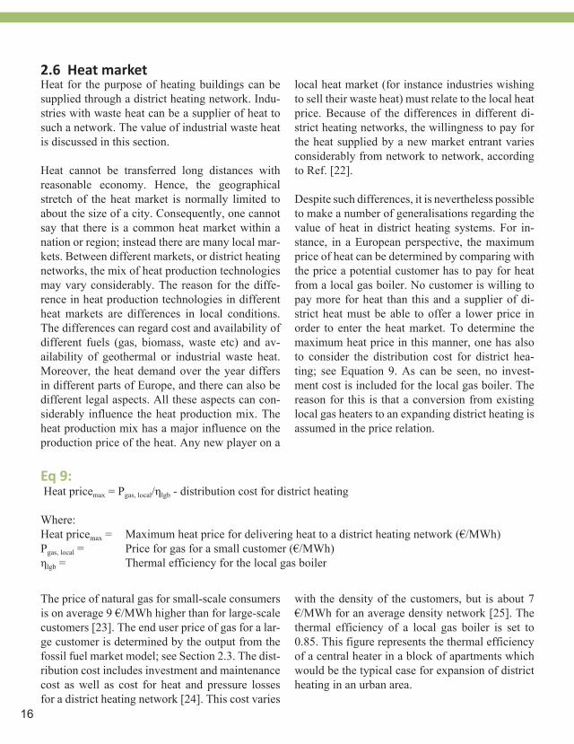
Eq 9: Heat pricemax = Pgas, local/ηlgb - distribution cost for district heating

Where:Heat pricemax = Maximum heat price for delivering heat to a district heating network (€/MWh)Pgas, local = Price for gas for a small customer (€/MWh)ηlgb = Thermal efficiency for the local gas boiler

The price of natural gas for small-scale consumers is on average 9 €/MWh higher than for large-scale customers [23]. The end user price of gas for a lar-ge customer is determined by the output from the fossil fuel market model; see Section 2.3. The dist-ribution cost includes investment and maintenance cost as well as cost for heat and pressure losses for a district heating network [24]. This cost varies

with the density of the customers, but is about 7 €/MWh for an average density network [25]. The thermal efficiency of a local gas boiler is set to 0.85. This figure represents the thermal efficiency of a central heater in a block of apartments which would be the typical case for expansion of district heating in an urban area.

17

By comparing with the heat production price for a local gas boiler, the maximum willingness to pay for heat delivery to a district heating system can be identified. However, the production cost for district heat can be lower than this. Hence, new players on the heat market, such as industries with waste heat, cannot always assume this maximum price. To obtain a reasonable lower price of heat, a technology with a low heat production cost can be considered. One such technology that is common in district heating systems in Europe is coal CHP [25]. Also large coal power plants can supply heat if a small part of the steam is extracted from the condensing turbine. However, these units are not assumed to be price setting for heat in the same degree as coal CHP plants.

The heat price in a coal CHP plant can be determi-ned according to Equation 10. As can be seen in the equation, investments costs are not included.

The reason is that a new player on an existing heat market would probably have to compete with the running cost of an existing heat producer. Using the plant data in Table 4, the heat price can thus be determined. This price can be used as a lower limit for a heat price span where the upper limit is set by Equation 9. Hence, the price from Equation 10 is denoted minimum heat price. Other technologies than coal CHP can a give higher heat prices than the one from Equation 10. But technologies with a higher price than the one from Equation 9 are not competitive. Hence, a new player on the heat mar-ket would have to compete with heat prices below the maximum heat price down to the minimum heat price. It should be mentioned that the heat price can be zero, for instance from waste incine-ration plants. Special cases like this are, however, not regarded here, since a new player would not be interested in selling the heat to zero price.

Eq 10: Heat pricemin = Pfuel

. (1+α)/ηtot-α. Pel + CO&M

Where: Heat pricemin = Minimum heat price for delivering heat to a district heating network (€/MWh)Pfuel = Fuel price including CO2 charge (€/MWh)α= ElectricitytoheatratiooftheCHPunitηtot = Total efficiency of the CHP plantPel = Economic value of cogenerated electricity (€/MWh), i.e. the electricity price accor-

ding to the electricity market model in the toolCO&M = Operating and maintenance cost (€/yr)

Table 4: Data for a coal CHP plant

α ηtot CO&M

Coal CHP 0,55 0,88 4 €/MWhheat

The intention with these minimum and maximum heat prices is to determine the span of heat prices that a new player on an existing heat market would

have to compete with. A new player could typical-ly be an industry wanting to sell their waste heat. Experience from the Swedish market shows that

18

the price an industry is paid for their waste heat is often lower than the marginal production cost for established district heat suppliers [22]. Moreover, the load and annual time of heat deliveries vary significantly from case to case. These experiences should be taken into consideration when the figu-res presented here are used, i.e. it is important not to overestimate the value of waste heat from an industrial plant.

The willingness to pay for waste heat according to Equation 9 and 10 does not include any invest-ments for piping to a new player. It is however likely that new piping to the industrial site would be needed, but since this cost is very site specific it is not included in the willingness to pay values presented here. Instead the user of the tool has to take this cost into consideration separately.

With the method described above, the maximum and minimum values for the e.g. waste heat from an industrial supplier can be found. Waste heat of this kind can be considered CO2 neutral since no

additional fuel is used for the production of this by-product. Hence, deliveries of waste heat would decrease the CO2 emissions in the heat system if the heat production is otherwise associated with CO2 emissions. The CO2 emissions associated to the replacement of a local gas boiler (maximum heat price in Equation 9) can be related to the use of gas. In the case of replacement of coal CHP (minimum heat price in Equation 10), the CO2 emissions are of course related to the use of coal, but in this case the CO2 emissions of the margi-nal electricity production must also be considered since the electricity production decreases.

With these approaches, CO2 emissions can be as-sociated to the minimum and maximum heat price. However, it should be noted that the CO2 emis-sions for the marginal heat production can differ considerably to these ones, if the heat production system has other technologies than presented here. For instance the emissions can be negative if the heat production is dominated by CHP based on wood fuel (which is quite common in Sweden).

19

3. Eight scenarios from 2010 to 2050

The principles described in the previous chapter were used to develop eight different energy market scenarios for the time period 2010-2050. All sce-narios start with the same value for the year 2010 and thereafter develop in eight different directions; the principle is illustrated in Figure 4. As can be seen in the figure, the eight scenarios are achieved by combining high and low fossil prices with four levels of CO2 emissions charge. This set of two

times four values of input data are needed for each calculation point from 2020 to 2050. For 2010, only one set of data is used since this is the starting point of the scenarios. In the following subsection, the input data used are presented and in Section 3.2 the resulting energy market scenarios are des-cribed. All input data and resulting energy market parameters are also presented in Appendix A.

Figure 4: Example illustrating the principle for the eight scenarios. By combining two levels of fossil fuel prices and four levels of CO2 charge, eight different combinations of input data are achieved, yielding eight scenarios for years 2020 to 2050. For the year 2010 only one set of input data is used, giving the starting point for all scenarios.

20

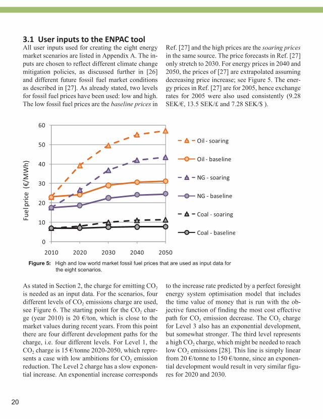
All user inputs used for creating the eight energy market scenarios are listed in Appendix A. The in-puts are chosen to reflect different climate change mitigation policies, as discussed further in [26] and different future fossil fuel market conditions as described in [27]. As already stated, two levels for fossil fuel prices have been used: low and high. The low fossil fuel prices are the baseline prices in

Ref. [27] and the high prices are the soaring prices in the same source. The price forecasts in Ref. [27] only stretch to 2030. For energy prices in 2040 and 2050, the prices of [27] are extrapolated assuming decreasing price increase; see Figure 5. The ener-gy prices in Ref. [27] are for 2005, hence exchange rates for 2005 were also used consistently (9.28 SEK/€, 13.5 SEK/£ and 7.28 SEK/$ ).

3.1 User inputs to the ENPAC tool

Figure 5: High and low world market fossil fuel prices that are used as input data for the eight scenarios.

As stated in Section 2, the charge for emitting CO2 is needed as an input data. For the scenarios, four different levels of CO2 emissions charge are used, see Figure 6. The starting point for the CO2 char-ge (year 2010) is 20 €/ton, which is close to the market values during recent years. From this point there are four different development paths for the charge, i.e. four different levels. For Level 1, the CO2 charge is 15 €/tonne 2020-2050, which repre-sents a case with low ambitions for CO2 emission reduction. The Level 2 charge has a slow exponen-tial increase. An exponential increase corresponds

to the increase rate predicted by a perfect foresight energy system optimisation model that includes the time value of money that is run with the ob-jective function of finding the most cost effective path for CO2 emission decrease. The CO2 charge for Level 3 also has an exponential development, but somewhat stronger. The third level represents a high CO2 charge, which might be needed to reach low CO2 emissions [28]. This line is simply linear from 20 €/tonne to 150 €/tonne, since an exponen-tial development would result in very similar figu-res for 2020 and 2030.

21

0

50

100

150

2000 2010 2020 2030 2040 2050 2060

Level 4

Level 3

Level 2

Level 1

CO2

char

ge (€

/ton

ne)

Figure 6: The four levels of CO2 charge that is used as input data for the eight scenarios.

The support for electricity production from wood fuel (see Section 2.2) varies throughout Europe, but can be set to 20 €/MWhel to represent an av-erage value for Europe [10].

As stated in Section 2.4, the availability of carbon capture and storage technology in the electricity market model of the ENPAC tool is set by the user. In this case with continuous scenarios, this parameter is used to decide when this technology is assumed to be available in full scale. CCS is as-sumed to be available to some extent by 2020 but will probably not be the dominating build margin by then [29]. Consequently, CCS is considered to be an available build margin technology (see Sec-tion 2.4) from 2030 and onwards.

The results for the starting point for the scenarios, 2010, are derived in the same way as the other en-

ergy market parameters, besides the fact that there is only one set of input data for this year. The in-put of world market fossil fuel prices and the CO2 charge for 2010 are figures close to the prices of the time of writing; see Appendix A. These figures are used in the tool to obtain consistent prices for electricity, wood fuel and heat for 2010.

Even though the input data are close to the current ones at the time of writing, they are likely to ra-pidly change in the short term given the significant short time fluctuations in market energy prices. These fluctuation are however not relevant. In fact the energy prices for 2010 are barely relevant at all, since the purpose of the scenario package is to evaluate future investments (see the introduction). However, any user of the tool can choose other data for 2010 to reflect a more updated situation if desired.

22

3.2 Resulting scenariosThe resulting energy market scenarios are presen-ted in brief below with one energy market in each subsequent subsection. All the detailed results are presented in Appendix A. No deep or detailed ana-

lysis of the resulting energy market scenarios are given below, since all the principles and relations are already discussed in the previous section.

3.2.1 Fossil fuel marketAll the resulting fossil fuel prices for a large custo-mer are presented in Appendix A, and the results are exemplified in Figure 7. As can be seen, the fuel oil prices vary over a wide span. In the sce-narios with low world market fossil fuel prices and low CO2 emissions charge, the end user prices

only increase slightly from 2010 to 2050. In the scenarios with opposite conditions, the end user prices increase to up to the triple. These general results are also applicable for the other fuel types; see Appendix A.

Figure 7: ENPAC light fuel oil price for a large customer.

3.2.2 Electricity marketIn Figure 8 the results for the electricity market are presented. As can be seen, the wholesale electricity price increases with the CO2 emissions charge and the fossil fuel price. With the intro-duction of carbon capture and storage technolo-gy, however, the increase of the electricity price due to increased CO2 emissions charge can be

moderate (see lines for CO2 charge of level 3 and 4 from year 2030). For CCS to be profitable, the CO2 charge must be at least 45-55 €/tonne. Be-fore CCS is available in large scale (2010-2020), natural gas combined cycles (NGCC) can be a profitable option if the CO2 emissions charge is high enough.

23

18

36

54

72

90

5

10

15

20

25

2010 2020 2030 2040 2050

High - level 4

Low - level 4

High - level 3

Low - level 3

High - level 2

Low - level 2

High - level 1

Low - level 1

€/G

J

€/M

Wh

Wholesale electricity priceFossil fuel price - CO2 charge

Broken lines = High fossil fuel pricesCon�nuous lines = Low fossil fuel prices

Figure 8: ENPAC wholesale electricity prices.

As explained in Section 2.5, two different margi-nal users for wood fuel have been considered: coal power plants (with and without support for rene-wable electricity) and producers of biofuel. All results are presented in Appendix A and in Figure 9 the results are exemplified for co-combustion in coal power plants with support for renewable elec-tricity. As can be seen in the figure, the wood fuel prices are heavily dependent on the CO2 charge. However, the difference between high and low coal price is too small to make a big difference.

If the coal power plants do not benefit from policy instruments in support of renewable electricity generation, the wood fuel prices follow the same trend but are about 10 €/MWh lower; see Appen-dix A. These results are very similar to those ac-hieved assuming that the marginal user of biomass feedstock is producers of biofuel, but two princi-ple differences can be identified: 1) the fossil fuel price (oil price) is more decisive in this case, and 2) the CO2 emissions related to marginal use of wood fuel is smaller.

3.2.3 Wood fuel market

24

Figure 9: ENPAC market price of low grade wood fuel if coal power plants with support for renewable electricity are the marginal user.

As discussed in Section 2.6, the heat price that a new player entering the heat market would face would be somewhere between a minimum and a maximum price, see Figure 10. The results are

exemplified for the scenario with low fossil fuel prices and level 2 CO2 charge; the results for all scenarios are found in Appendix A.

3.2.4 Heat market

Figure 10: ENPAC price span for heat for a new player (e.g. supplier of industrial waste heat) entering a heat market in the scenario with low fossil fuel prices and level 2 CO2 charge.

25

4. References

[1] IEA, Energy Technology Perspectives 2008 - Scenarios and Strategies to 2050, ISBN 978-92-64-04142-4, IEA Publications, Paris, 2008.

[2] IEA, Tracking Industrial Energy Efficiency and CO2 Emissions. IEA Publications, Paris, 2007.

[3] Ådahl A., Harvey S., Energy efficiency investments in kraft pulp mills given uncertain climate policy, Int. J. of Energy Research 31(5): pp 486-505, 2007.

[4] Darton R., Scenario Building and Uncertainties: Options for Energy Sources. Chapter in: Azapagic A., Perdan S., Clift R., Sustainable Development in Practice, West Sussex: John Wiley & Sons Ltd. pp. 301-320. 2004.

[5] Ådahl, A., Process industry energy projects in a climate change conscious economy, PhD thesis, Heat and Power Technology, Dept. of Chemical Engineering and Environmental Science. Chal mers University of Technology, Göteborg, Sweden.

[6] Axelsson, E., Energy Export Opportunities from Kraft Pulp and Paper Mills and Resulting Reductions in Global CO2 Emissions, PhD thesis, Dept. of Energy and Environment, Chalmers University of Technology, Göteborg, Sweden.

[7] Axelsson E., Harvey S., Berntsson T., A tool for creating energy market scenarios for evaluation of investments in energy intensive industry, Energy, Volume 34 (Issue 12) s. 2036-2074, 2009. Published online: http://dx.doi.org/10.1016/j.energy.2008.08.017.

[8] European Energy Agency, Annual European Community greenhouse gas inventory 1990–2006 and inventory report 2008, Technical report No 6/2008, 2008.

[9] Commission of the European Community, The support of electricity from renewable energy sources, COM(2005) 627 final, 2005.

[10] Fouquet D., Prices for Renewable Energies in Europe: Feed-in tariffs versus Quota Systems – a comparison, EREF report, 2007.

[11] Energimyndigheten, Energy in Sweden Facts and Figures 2007, report from The Swedish Energy Agency, 2007. Available online at www.swedishenergyagency.se.

26

[12] Uppenberg et al., Environmental Handbook for Fuels (Miljöfaktaboken för Bränslen). IVL report B1334A-2, Stockholm, Sweden, 2001 (in Swedish).

[13] Sköldberg H., Unger T., Olofsson M., Marginal Electricity and Evaluating the Environmental Impact of Electricity (Marginalel och miljövärdering av el). Elforsk report 06:52, Stockholm, Sweden, 2006 (in Swedish). Available online at www.elforsk.se.

[14] Odenberger M., Kjärstad J., Johnsson F., Ramp up of CO2 Capture and Storage within Europe, International Journal of Greenhouse Gas Control, 4(2): pp 417-438, 2008.

[15] IEA Bioenergy Task 40, Opportunities and barriers for sustainable international bioenergy trade and strategies to overcome them, a report prepared by IEA Bioenergy Task 40, 2006. Available online at www.bioenergytrade.org.

[16] Johnsson, F., Berndes, G., Berggren, M., Cost competitive bioenergy: linking lignocellulosic biomass supply with co-firing for electricity in Poland. Presented at World Bioenergy Conference and Exhibition, Jönköping, Sweden, 30 May–1 June 2006.

[17] Berndes G., Magnusson L., The future of bioenergy in Sweden, Report no. ER 2006:30, Swedish Energy Agency, 2006. Available online at www.swedishenergyagency.se.

[18] Boding H., Ahlvik P., Brandber Å., Ekbom T., BioMeeT II – Stakeholders for biomass based Methanol/DME/Power/Heat energy combine, Eco-traffic and Nykomb Synergetics, 2003. Available online at www.nykomb.se.

[19] Hedenus F., Karlsson S., Azar C., Sprei F., The transportation energy carrier of the future - System interactions between the transportation and stationary sectors in a carbon constrained world, presented at EVS24 Towards Zero Emissions, Stavanger, Norway, 2009.

[20] Biomass Fuel Atlas of Profu, 2009.

[21] Energimyndigheten, Price Statistics for Biomass Fuels, Peat, etc (Prisblad för biobränsle, torv mm), nr 4 2008. Available online at www.swedishenergyagency.se.

[22] Personal communication, John Johnsson, Senior consultant at Profu i Göteborg AB, 2008.

[23] Eurostat, Energy statistics from the European Commission, 2009. Available online at www.epp.eurostat.ec.europa.eu.

[24] Fredriksson S., Werner S., Fjärrvärme – teori, teknik och funktion, Studentlitteratur, Lund, 1993.

27

[25] Werner S., Possibilities with more district heating in Europe - report of Ecoheatcool work Package 4, Euroheat & Power, 2006. Available online at www.euroheat.org.

[26] Ådahl A., Harvey S., Berntsson T. Assessing the value of pulp mill biomass savings in a climate change conscious economy, Energy Policy 34(15): pp 2330-2343, 2006.

[27] Capros P., Mantzos L., Papandreou V., Tasios N., Energy and transport: Trends to 2030 - update 2007, European Comission: Directorate-General for Energy and Transport, 2008.

[28] Mantzos L., Capros P., Zeka–Paschou M., European energy and transport scenarios on key drivers, Directorate-General for Energy and Transport, 2004.

[29] ENCAP, Power systems evaluation and benchmarking, ENCAP report D1.2.4 , 2008.

29

Here all the input data and resulting energy market parameters are presented in tables according to the list below:

Input data: Table A1Fossil fuel market: Table A2Electricity market: Table A3Bioenergy market: Table A4:1-Table A4:3Heat market: Table A5:1-Table A5:2

Table A1: Input data for the energy market scenarios

Fossil fuel prices1 (€/MWh) 2010 2020 2030 2040 2050

Oil low 23 24 29 31 31

high 23 39 49 55 57

Natural gas low 18 19 22 24 25

high 18 27 37 42 44

Coal low 7,0 7,1 7,5 7,6 7,7

high 7,0 8 10 11 11

Policy instruments

CO2 emission charge (€/ton) level 1 20 15 15 15 15

level 2 20 20 27 37 50

level 3 20 30 45 68 101

level 4 20 52 85 117 150

RES-E support 2 (€/MWh) 20 20 20 20 20

Technology availability

CCS available no no yes yes yes

1 On the world market2 Premium paid to producers of renewable electricity from combustible renewables (above market electricity price)

Appendix A – Input data and resulting energy market parameters

30

Table A2 : Resulting end-user fossil fuel prices, including CO2 charge (€/MWh)

Fossil fuel price* CO2 charge 2010 2020 2030 2040 2050

Light fuel oil low level 1 44 44 49 51 51

low level 2 44 45 53 57 62

low level 3 44 48 58 66 77

low level 4 44 54 70 81 91

high level 1 44 61 72 79 81

high level 2 44 62 76 85 91

high level 3 44 65 81 94 106

high level 4 44 72 93 109 121

Heavy fuel oil

low level 1 28 27 31 33 33

low level 2 28 29 35 39 43

low level 3 28 32 40 48 58

low level 4 28 38 52 63 73

high level 1 28 40 49 54 55

high level 2 28 42 52 60 66

high level 3 28 44 58 69 81

high level 4 28 51 70 84 95

Natural gas low level 1 26 26 30 32 32

low level 2 26 27 33 36 40

low level 3 26 29 37 43 51

low level 4 26 34 45 54 61

high level 1 26 34 44 50 51

high level 2 26 35 47 54 59

high level 3 26 37 51 61 70

high level 4 26 42 60 72 80

* On the world market, see input data

31

[continued] Table A2 : Resulting end-user fossil fuel prices, including CO2 charge (€/MWh)

Fossil fuel price* CO2 charge 2010 2020 2030 2040 2050

Coal low level 1 14 13 14 14 14

low level 2 14 15 18 21 26

low level 3 14 18 24 32 44

low level 4 14 26 38 49 61

high level 1 14 14 16 17 17

high level 2 14 16 20 25 30

high level 3 14 19 26 35 47

high level 4 14 27 40 52 64

* On the world market, see input data

32

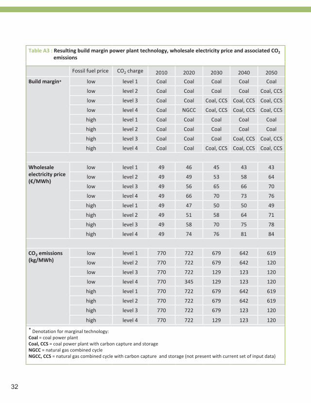
Table A3 : Resulting build margin power plant technology, wholesale electricity price and associated CO2 emissions

Fossil fuel price CO2 charge 2010 2020 2030 2040 2050

Build margin* low level 1 Coal Coal Coal Coal Coal

low level 2 Coal Coal Coal Coal Coal, CCS

low level 3 Coal Coal Coal, CCS Coal, CCS Coal, CCS

low level 4 Coal NGCC Coal, CCS Coal, CCS Coal, CCS

high level 1 Coal Coal Coal Coal Coal

high level 2 Coal Coal Coal Coal Coal

high level 3 Coal Coal Coal Coal, CCS Coal, CCS

high level 4 Coal Coal Coal, CCS Coal, CCS Coal, CCS

Wholesale electricity price (€/MWh)

low level 1 49 46 45 43 43

low level 2 49 49 53 58 64

low level 3 49 56 65 66 70

low level 4 49 66 70 73 76

high level 1 49 47 50 50 49

high level 2 49 51 58 64 71

high level 3 49 58 70 75 78

high level 4 49 74 76 81 84

CO2 emissions(kg/MWh)

low level 1 770 722 679 642 619

low level 2 770 722 679 642 120

low level 3 770 722 129 123 120

low level 4 770 345 129 123 120

high level 1 770 722 679 642 619

high level 2 770 722 679 642 619

high level 3 770 722 679 123 120

high level 4 770 722 129 123 120

* Denotation for marginal technology:Coal = coal power plant Coal, CCS = coal power plant with carbon capture and storageNGCC = natural gas combined cycle NGCC, CCS = natural gas combined cycle with carbon capture and storage (not present with current set of input data)

33

Table A4:1 – A4:3. Market price2 for wood fuels and associated CO2 emissions.

Table A4:1 : If coal power plants benefitting from support of renewable electricity production are the marginal user of wood fuel


Low grade* (€/MWh)

low level 1 20 20 21 22 22

low level 2 20 22 25 29 34

low level 3 20 25 31 40 52

low level 4 20 33 45 57 69

high level 1 20 21 23 25 26

high level 2 20 23 28 33 38

high level 3 20 26 34 43 56

high level 4 20 34 48 60 73

Pellets (€/MWh)

low level 1 31 31 32 33 34

low level 2 31 33 38 43 50

low level 3 31 38 46 57 72

low level 4 31 48 64 79 94

high level 1 31 32 36 38 39

high level 2 31 35 41 48 54

high level 3 31 39 49 61 77

high level 4 31 49 67 83 99

CO2 emissions, all scenarios 336 kg/MWh

* Low grade biofuel such as tops and branches, sawdust etc.

2) i.e. buyers price. To get sellers price, the transportation cost (of e.g. 4.3 €/MWh) most to be deducted.

34

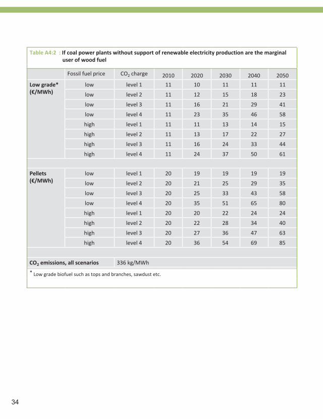
Table A4:2 : If coal power plants without support of renewable electricity production are the marginal user of wood fuel



low level 1 11 10 11 11 11

low level 2 11 12 15 18 23

low level 3 11 16 21 29 41

low level 4 11 23 35 46 58

high level 1 11 11 13 14 15

high level 2 11 13 17 22 27

high level 3 11 16 24 33 44

high level 4 11 24 37 50 61

Pellets (€/MWh)

low level 1 20 19 19 19 19

low level 2 20 21 25 29 35

low level 3 20 25 33 43 58

low level 4 20 35 51 65 80

high level 1 20 20 22 24 24

high level 2 20 22 28 34 40

high level 3 20 27 36 47 63

high level 4 20 36 54 69 85


* Low grade biofuel such as tops and branches, sawdust etc.

35

Table A4:3 : If producers of biofuel are the marginal user of wood fuel



low level 1 -4,2 -4,0 0 1 2

low level 2 -4,2 -3,3 1 4 7

low level 3 -4,2 -1,9 4 9 16

low level 4 -4,2 2 11 18 24

high level 1 -4,2 8 15 20 21

high level 2 -4,2 8 17 23 26

high level 3 -4,2 10 20 28 35

high level 4 -4,2 13 27 37 44

Pellets (€/MWh)

low level 1 0 0 5 7 7

low level 2 0 1 7 11 14

low level 3 0 3 11 18 26

low level 4 0 7 20 29 37

high level 1 0 15 25 31 33

high level 2 0 16 28 35 40

high level 3 0 18 31 42 51

high level 4 0 22 40 53 62

CO2-emissions (kg/MWh)

low level 1 112 115 118 120 121

low level 2 112 115 118 120 153

low level 3 112 115 152 152 153

low level 4 112 139 152 152 153

high level 1 112 115 118 120 121

high level 2 112 115 118 120 121

high level 3 112 115 118 152 153

high level 4 112 115 152 152 153

* Low grade wood fuel such as tops and branches, sawdust etc.

36

Table A5:1 – A5:2. Market value for sales of heat to a district heating network and associated CO2 emissions.

Table A5:1 : Minimum market value (related to heat production price in a coal-fired CHP plant)


Heat price (€/MWh)

low level 1 3,6 2,2 3,4 4 5

low level 2 3,6 3,3 6,2 10 15

low level 3 3,6 5,4 11 24 42

low level 4 3,6 14 32 51 69

high level 1 3,6 2,8 5,1 6,8 7,7

high level 2 3,6 3,9 7,9 12 17

high level 3 3,6 6,0 12 25 44

high level 4 3,6 11 33 52 71

CO2 emissions(kg/MWh)

low level 1 187 213 237 257 270

low level 2 187 213 237 257 544

low level 3 187 213 539 543 544

low level 4 187 421 539 543 544

high level 1 187 213 237 257 270

high level 2 187 213 237 257 270

high level 3 187 213 237 543 544

high level 4 187 213 539 543 544

37

Table A5:1 : Maximum market value (related to heat production price in local gas boilers)


Heat price (€/MWh)

low level 1 34 34 39 41 41

low level 2 34 36 42 46 50

low level 3 34 38 47 54 63

low level 4 34 44 57 67 76

high level 1 34 44 56 62 64

high level 2 34 45 59 68 73

high level 3 34 48 63 75 86

high level 4 34 53 74 88 98


39

Appendix B – Suggestions for short descriptions of the scenarios for use in reports, papers, etc where output values from the scenarios are used as input in cal-culations The authors of this report assume that most sce-nario users will use output values generated by the ENPAC tool as input data in calculations for which the results will be presented in reports, sci-entific papers, etc. In such cases it is often neces-sary to include a brief summary of the assumptions and calculation methods included in the tool. Pro-viding such a short description of the ENPAC tool and results might be difficult for someone who has not been involved in the development of them. Hence, four suggestions with different lengths on how the scenarios can be described are given be-low.

Two sentencesThe performance of future or long-term energy in-vestments at industrial sites can be evaluated using consistent scenarios. By using a number of diffe-rent scenarios that outline possible cornerstones of the future energy market, robust investments can be identified.

One paragraphThe performance of future or long-term energy in-vestments at industrial sites can be evaluated using consistent scenarios. By using a number of diffe-rent scenarios that outline possible cornerstones of the future energy market, robust investments can be identified and the climate benefit can be evalua-ted. To obtain reliable results, it is important that the energy market parameters within a scenario are consistent. Consistent scenarios can be achieved by using a tool in which the energy-market para-meters (e.g. energy prices and energy conversion technologies) are related to each other.

Half a pageTo assess profitability and net CO2 emissions re-duction potential of strategic energy-related in-vestments in the industrial sector, it is important to consider possible developments of future energy market conditions. Scenarios including future en-ergy prices can be used to reflect different possible future energy market conditions. By assessing the profitability of investments for different energy market conditions, it is easier to identify robust investment options.

To achieve reliable results from the economic as-sessment, the energy market parameters within a given scenario must be consistent, i.e. the energy prices must be related to each other (i.e. accoun-ting for energy conversion technology characte-ristics and applying suitable substitution princip-les). A systematic approach for constructing such consistent scenarios requires the use of a suitable calculation tool. In this report the Energy Price and Carbon Balance Scenarios tool (the ENPAC tool) is used. The ENPAC tool proposes energy market prices for large-volume customers, based on world market fossil fuel price data and assumed values for energy and climate mitigation policy in-struments. Hence, required user inputs to the tool include fossil fuel prices and charge for emitting CO2.

With these inputs, the probable marginal energy conversions technologies in key energy markets can be determined, which in turn yield consistent values for energy prices and CO2 emissions asso-ciated with marginal use of key energy carriers,

namely fossil fuels, electricity, wood fuel and heat for district heating.

Using the ENPAC tool, eight scenarios for the time period from 2010 to 2050 have been develo-ped. The eight scenarios are a result of combining two levels of fossil fuel prices and four level of CO2 charge. Two levels of fossil fuel prices re-present different developments on the fossil fuel

world market. Four levels of CO2 emission charge represent everything from no to strong ambitions to decrease CO2 emissions.

About one pageUse the summary in the beginning of this report (possible including Figure 1 and/or Figure 2).

Pathways to sustainable European energy systemsThe European pathways project is a five year project with the overall aim to evaluate and propose robust pat-hways towards a sustainable energy system with respect to environmental, technical, economic and social issues. The focus is on the stationary energy system (power and heat) in the European setting. Evaluations will be based on a detailed description of the present energy system and follow how this can be developed into the future under a range of environmental, economic and infrastructure constraints. The proposed project is a response to the need for a large and long-term research project on European energy pathways, which can produce independent results to support decision makers in industry and in govern-mental organizations. Stakeholders for this project are: the European utility industry and other energy related industries, the European Commission, EU-Member State governments and their energy related boards and oil and gas companies. The overall question to be answered by the project is:

How can pathways to a sustainable energy system be characterized and visualized and what are the consequen-ces of these pathways with respect to the characteristics of the energy system as such (types of technologies, technical and economic barriers) and for society in general (security of supply, competitiveness and required policies)?

This question is addressed on three levels; by means of energy systems analysis (technology assessment and technical-economic analysis), a multi-disciplinary analysis and an extended multi-disciplinary policy analysis. From a dialogue with stakeholders, the above question has been divided into sub-questions such as:

• Whatisthecriticaltimingfordecisionstoensurethatapathway to a sustainable energy system can be followed?

• Whatare”key”technologiesandsystemsfortheidentified”pathways”-includingidentificationof uncertainties and risks for technology lock-in effects?

• Whatrequirementsandconsequencesareimposedon the energy system in case of a high penetration of renewables?

• Whataretheconsequencesofastrongincreaseintheuse of natural gas?

• WhatifeffortstodevelopCO2 capture and storage fail?

• Whereshouldbiomassbeused–inthetransportationsector or in the stationary energy system?

• Arethederegulatedenergymarketssuitabletofacilitatea development towards a sustainable energy system?

• Willenergyefficiencybeachievedthroughfreemarketforces or regulatory action?

• Whataretherequirementsoffinancingtheenergy infrastructure for the different pathways identified?

In order to address the sub-questions in an efficient and focussed way the project is structured into 10 work packages addressing topics such as description of the energy infrastructure, energy systems modelling, tech-nology assessment of best available and future technologies and international fuel markets. In planning of the project significant efforts have been put into ensuring that the project should not only be strong in research but also in management, communication and fundraising.

The global dimension will be ensured through integration with the other three regional AGS pathway projects in the Americas, East Asia, and India and Africa.

More information at Pathways website:www.energy-pathways.org

43

The Alliance for Global Sustainability (AGS) brings togetherfouroftheworld’sleadingtechnicaluniversities–Massachusetts Institute of Technology, The University of Tokyo, Chalmers University of Technology and the Swiss FederalInstituteofTechnology–toconductresearchincollaboration with government and industry on some of society´s greatest challenges.

The AGS represent a new synthesis of multidisciplinary and multi-geographical research that draws on the diverse

and complementary skills of the AGS partners. In addi-tion to academic collaborations each of the universities has extensive experience in working with stakeholders, particularly a growing number of visionary leaders from industry who recognise their fundamental role in achieving sustainable development.

More information at AGS website: globalsustainability.org

The Alliance for Global Sustainability

Foto: Måns Ahnlund

European energy infrastructure - the Chalmers databases 2006 The AGS Pathways reports 2006:EU1

The carbon dioxide free power plant - large scale capture and storage of carbon dioxide. process evaluation and test-facility measurements

The AGS Pathways reports 2006:EU2

Multifunctional bioenergy systemsThe AGS Pathways reports 2007:EU1

Public and stakeholder attitudes towards energy, environment and CCS The AGS Pathways reports 2007:E2

Co-combustion, a summary of technologyThe AGS Pathways reports 2007:E3

The reports can be ordered from:

AGS Office at Chalmers

GMV, Chalmers

SE - 412 96 Göteborg

[email protected]

The AGS Pathways reports

FOUR UNIVERSITIES

The Alliance for Global Sustainability is an international part-

nership of four leading science and technology universities:

CHALMERS Chalmers University of Technology, was founded

in 1829 following a donation, and became an independent

foundation in 1994.Around 13,100 people work and study at

the university. Chalmers offers Ph.D and Licentiate course pro-

grammes as well as MScEng, MArch, BScEng, BSc and nautical

programmes.

Contact: Alexandra Priatna

Phone: +46 31 772 4959 Fax: +46 31 772 4958


ETH Swiss Federal Institute of Technology Zurich, is a science

and technology university founded in 1855. Here 18,000 people

from Switzerland and abroad are currently studying, working or

conducting research at one of the university’s 15 departments.

Contact: Peter Edwards

Phone: +41 44 632 4330 Fax: +41 44 632 1215


MIT Massachusetts Institute of Technology, a coeducational,

privately endowed research university, is dedicated to advanc-

ing knowledge and educating students in science, technology,

and other areas of scholarship. Founded in 1861, the institute

today has more than 900 faculty and 10,000 undergraduate

and graduate students in five Schools with thirty-three degree-

granting departments, programs, and divisions.

Contact: Karen Gibson

Phone: +1 617 258 6368 Fax: +1 617 258 6590


UT The Univeristy of Tokyo, established in 1877, is the oldest

university in Japan. With its 10 faculties, 15 graduate schools,

and 11 research institutes (including a Research Center for

Advanced Science and Technology), UT is a world-renowned,

research oriented university.

Contact: Yuko Shimazaki

Phone: +81 3 5841 7937 Fax: +81 3 5841 2303




PATHWAYS TO SUSTAINABLE EUROPEAN ENERGY SYSTEMS

SC

EN

AR

IOS

FOR

AS

SE

SS

ING

INV

ES

TME

NTS

IN IN

DU

STR

Y

Scenarios for assessing profitability and carbon balances of energy investments in industry

The performance of future or long-term energy investments at industrial sites can be eva-luated using consistent scenarios. By using a number of different scenarios that outline pos-sible cornerstones of the future energy market, robust investments can be identified and the climate benefit can be evaluated. Consistent scenarios can be achieved by using the Energy Price and Carbon Balance Scenarios tool (the ENPAC tool) which is presented here. The tool is also used to develop eight scenarios from 2010 to 2050 with energy prices and associated CO2 emissions for marginal use of the energy carriers.

This report is a result from the project Pathways to Sustainable European Energy Systems – a five year project within The AGS Energy Pathways Flagship Program.

The project has the overall aim to evaluate and propose ro bust pathways towards a sustainable energy system with respect to environ mental, tech nical, economic and social issues. Here the focus is on the stationary energy system (power and heat) in the European setting.

The AGS is a collaboration of four universities that brings together world-class ex-pertise from the member institutions to develop research and edu cation in collaboration with government and industry on the challenges of sustainable development.

THE

AG

S PATH

WAY R

EP

OR

TS 2010:E

U1

Example illustrating eight scenarios for the electricity price. By combining two levels of fossil fuel prices and four levels of CO2 charge, eight different combinations of input data are achieved, yielding eight scenarios for years 2020 to 2050. For the year 2010 only one set of input data is used, giving the starting point for all scenarios.

scenarios for assessing profitability and carbon balances of energy

Documents