schaum's outlines of signals & systems (ripped by sabbanji) · pdf filechap. 31...

Chapter 3

Laplace Transform and Continuous-Time LTI Systems

3.1 INTRODUCTION

A basic result from Chapter 2 is that the response of an LTI system is given by convolution of the input and the impulse response of the system. In this chapter and the following one we present an alternative representation for signals and LTI systems. In this chapter, the Laplace transform is introduced to represent continuous-time signals in the s-domain ( s is a complex variable), and the concept of the system function for a continuous-time LTI system is described. Many useful insights into the properties of continuous-time LTI systems, as well as the study of many problems involving LTI systems, can be provided by application of the Laplace transform technique.

3.2 THE LAPLACE TRANSFORM

In Sec. 2.4 we saw that for a continuous-time LTI system with impulse response h(t), the output y(0 of the system to the complex exponential input of the form e" is

where

A. Definition:

The function H ( s ) in Eq. (3.2) is referred to as the Laplace transform of h(t). For a general continuous-time signal x(t), the Laplace transform X(s) is defined as

The variable s is generally complex-valued and is expressed as

The Laplace transform defined in Eq. (3.3) is often called the bilateral (or two-sided) Laplace transform in contrast to the unilateral (or one-sided) Laplace transform, which is defined as

CHAP. 31 LAPLACE TRANSFORM AND CONTINUOUS-TIME LTI SYSTEMS 111

where 0-= lim,,,(O - E ) . Clearly the bilateral and unilateral transforms are equivalent only if x(t) = 0 for t < 0. The unilateral Laplace transform is discussed in Sec. 3.8. We will omit the word "bilateral" except where it is needed to avoid ambiguity.

Equation (3.3) is sometimes considered an operator that transforms a signal x( t ) into a function X(s) symbolically represented by

and the signal x( t ) and its Laplace transform X(s) are said to form a Laplace transform pair denoted as

B. The Region of Convergence:

The range of values of the complex variables s for which the Laplace transform converges is called the region of convergence (ROC). To illustrate the Laplace transform and the associated ROC let us consider some examples.

EXAMPLE 3.1. Consider the signal

x ( t ) =e-O1u(t) a real

Then by Eq. (3.3) the Laplace transform of x(t) is

because lim, ,, e-("'")' = 0 only if Re(s + a ) > 0 or Reb) > -a.

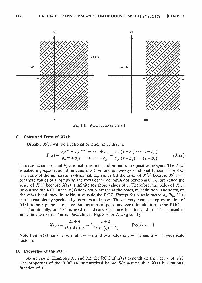
Thus, the ROC for this example is specified in Eq. (3.9) as Re(s) > -a and is displayed in the complex plane as shown in Fig. 3-1 by the shaded area to the right of the line Re(s) = -a. In Laplace transform applications, the complex plane is commonly referred to as the s-plane. The horizontal and vertical axes are sometimes referred to as the a-axis and the jw-axis, respectively.

EXAMPLE 3.2. Consider the signal

~ ( t ) = -e-"u( - t ) a real

Its Laplace transform X(s) is given by (Prob. 3.1)

Thus, the ROC for this example is specified in Eq. (3.11) as Re(s) < -a and is displayed in the complex plane as shown in Fig. 3-2 by the shaded area to the left of the line Re(s) = -a. Comparing Eqs. (3.9) and (3.11), we see that the algebraic expressions for X(s) for these two different signals are identical except for the ROCs. Therefore, in order for the Laplace transform to be unique for each signal x(t), the ROC must be specified as par1 of the transform.

LAPLACE TRANSFORM AND CONTINUOUS-TIME LTI SYSTEMS [CHAP. 3

s-plane

(a ) (b)

Fig. 3-1 ROC for Example 3.1.

C. Poles and Zeros of X ( s 1: Usually, X(s) will be a rational function in s, that is,

The coefficients a, and b, are real constants, and m and n are positive integers. The X(s) is called a proper rational function if n > m, and an improper rational function if n I m. The roots of the numerator polynomial, z,, are called the zeros of X(s) because X(s) = 0 for those values of s. Similarly, the roots of the denominator polynomial, p,, are called the poles of X(s) because X(s) is infinite for those values of s. Therefore, the poles of X(s) lie outside the ROC since X(s) does not converge at the poles, by definition. The zeros, on the other hand, may lie inside or outside the ROC. Except for a scale factor ao/bo, X(s) can be completely specified by its zeros and poles. Thus, a very compact representation of X(s) in the s-plane is to show the locations of poles and zeros in addition to the ROC.

Traditionally, an " x " is used to indicate each pole location and an " 0 " is used to indicate each zero. This is illustrated in Fig. 3-3 for X(s) given by

Note that X(s) has one zero at s = - 2 and two poles at s = - 1 and s = - 3 with scale factor 2.

D. Properties of the ROC:

As we saw in Examples 3.1 and 3.2, the ROC of X(s) depends on the nature of d r ) . The properties of the ROC are summarized below. We assume that X(s) is a rational function of s.

CHAP. 31 LAPLACE TRANSFORM AND CONTINUOUS-TIME LTI SYSTEMS

(a) (b)

Fig. 3-2 ROC for Example 3.2.

Fig. 3-3 s-plane representation of X ( s ) = (2s + 4)/(s2 + 4s + 3).

Property 1: The ROC does not contain any poles.

Property 2: If x ( t ) is a f initeduration signal, that is, x ( r ) = 0 except in a finite interval r , 5 r 2 r , ( - m < I , and I , < m), then the ROC is the entire s-plane except possibly s = 0 or s = E.

Property 3: If x ( t ) is a right-sided signal, that is, x ( r ) = 0 for r < r , < m, then the ROC is of the form


where a,,, equals the maximum real part of any of the poles of X(s). Thus, the ROC is a half-plane to the right of the vertical line Reb) = a,,, in the s-plane and thus to the right of all of the poles of Xb).

Property 4: If x(t) is a left-sided signal, that is, x(t) = O for t > t, > -=, then the ROC is of the form

where a,,, equals the minimum real part of any of the poles of X(s). Thus, the ROC is a half-plane to the left of the vertical line Re(s) =amin in the s-plane and thus to the left of all of the poles of X(s).

Property 5: If x(t) is a two-sided signal, that is, x(t) is an infinite-duration signal that is neither right-sided nor left-sided, then the ROC is of the form

where a, and a, are the real parts of the two poles of X(s). Thus, the ROC is a vertical strip in the s-plane between the vertical lines Re(s) = a, and Re(s) = a,.

Note that Property 1 follows immediately from the definition of poles; that is, X(s) is infinite at a pole. For verification of the other properties see Probs. 3.2 to 3.7.

3 3 LAPLACE TRANSFORMS OF SOME COMMON SIGNALS

A. Unit Impulse Function S( t ):

Using Eqs. (3.3) and (1.20), we obtain

J [ s ( t ) ] = /- s( t )e -" dt = 1 all s - m

B. Unit Step Function u ( t 1:

where O + = lim, , "(0 + €1.

C. Laplace Transform Pairs for Common Signals:

The Laplace transforms of some common signals are tabulated in Table 3-1. Instead of having to reevaluate the transform of a given signal, we can simply refer to such a table and read out the desired transform.

3.4 PROPERTIES OF THE LAPLACE TRANSFORM

Basic properties of the Laplace transform are presented in the following. Verification of these properties is given in Probs. 3.8 to 3.16.


Table 3-1 Some Laplace Transforms Pairs

1 All s

cos wotu(t)

sin wotu(t

s + a e-"' cos wotu(t) Re(s) > - Re(a)

( s + a 1 2 + w ;

A. Linearity:

If

The set notation A I B means that set A contains set B, while A n B denotes the intersection of sets A and B, that is, the set containing all elements in both A and B. Thus, Eq. (3.15) indicates that the ROC of the resultant Laplace transform is at least as large as the region in common between R , and R 2 . Usually we have simply R' = R , n R , . This is illustrated in Fig. 3-4.

LAPLACE TRANSFORM AND CONTINUOUS-TIME LTI SYSTEMS

iw

[CHAP.

Fig. 3-4 ROC of a , X , ( s ) + a , X , ( s ) .

B. Time Shifting:

If

) ' - * X ( S ) ROC = R

then x ( t - t o ) -e-"[)X ( s 1 R ' = R (3 .16)

Equation (3 .16) indicates that the ROCs before and after the time-shift operation are the same.

C. Shifting in the s-Domain:

If

then e+"x( t ) - X ( s - so ) R' = R + Re(so) ( 3 . 1 7 )

Equation (3.1 7 ) indicates that the ROC associated with X ( s - so) is that of X ( s ) shifted by Re(s,,). This is illustrated in Fig. 3-5.

D. Time Scaling:

I f

then

x ( t ) + + X ( S ) ROC = R

( R 1 = a R x ( a t ) - - X - la l

CHAP- 31 LAPLACE TRANSFORM AND CONTINUOUS-TIME LTI SYSTEMS

(4 (b)

Fig. 3-5 Effect on the ROC of shifting in the s-domain. ( a ) ROC of X(s); ( b ) ROC of X ( s - so).

Equation (3.18) indicates that scaling the time variable t by the factor a causes an inverse scaling of the variable s by l / a as well as an amplitude scaling of X ( s / a ) by I/ Jal. The corresponding effect on the ROC is illustrated in Fig. 3-6.

E. Time Reversal:

If

Fig. 3-6 Effect on the ROC of time scaling. (a) ROC of X(s ) ; ( b ) ROC of X(s/a).

118 LAPLACE TRANSFORM AND CONTINUOUS-TIME LTI SYSTEMS [CHAP. 3

then x ( - t ) *X(-S) R' = - R (3.19)

'Thus, time reversal of x( t ) produces a reversal of both the a- and jw-axes in the s-plane. Equation (3.19) is readily obtained by setting a = - 1 in Eq. (3.18).

F. Differentiation in the Time Domain:

If

~ ( t ) ++X(S) ROC = R

then

Equation (3.20) shows that the effect of differentiation in the time domain is multiplication of the corresponding Laplace transform by s. The associated ROC is unchanged unless there is a pole-zero cancellation at s = 0.

G. Differentiation in the s-Domain:

If

41) ++X(S) ROC = R

then -

H. Integration in the Time Domain:

If

then

Equation (3.22) shows that the Laplace transform operation corresponding to time-domain integration is multiplication by l/s, and this is expected since integration is the inverse operation of differentiation. The form of R' follows from the possible introduction of an additional pole at s = 0 by the multiplication by l/s.

I. Convolution:

1 f

x d l ) * w ) R O C = R ,

~ 2 ( 4 ++XZ(S) ROC = R2


Table 3-2 Properties of the Laplace Transform

Property Signal Transform ROC

x ( t ) X ( s ) R x , ( t ) x ,w R 1

x 2 W x,w R2 Linearity a , x , ( t ) + a 2 x 2 ( l ) a , X , ( s ) + a , X 2 ( s ) R ' I R , n R 2 Time shifting x(t - t o ) e-""X(s) R' = R Shifting in s es"'x( t X ( s - so) R' = R + Re(s,)

1 Time scaling x( at - X ( s ) R' = aR

la l Time reversal R ' = - R

Differentiation in t

Differentiation in s - t x ( t ) dX( s ) R f = R

ds

Integration

Convolution

then % ( t ) * ~ 2 0 ) H X I ( ~ ) X ~ ( ~ ) R ' I R , n R 2 (3.23)

This convolution property plays a central role in the analysis and design of continuous-time LTI systems.

Table 3-2 summarizes the properties of the Laplace transform presented in this section.

3.5 THE INVERSE LAPLACE TRANSFORM

Inversion of the Laplace transform to find the signal x ( t ) from its Laplace transform X(s) is called the inverse Laplace transform, symbolically denoted as

A. Inversion Formula:

There is a procedure that is applicable to all classes of transform functions that involves the evaluation of a line integral in complex s-plane; that is,

In this integral, the real c is to be selected such that if the ROC of X(s) is a, < Re(s) <a2, then a, < c < u2. The evaluation of this inverse Laplace transform integral requires an understanding of complex variable theory.


B. Use of Tables of Laplace Transform Pairs:

In the second method for the inversion of X(s), we attempt to express X(s) as a sum

X(s) = X,(s) + . . . +Xn(s) (3.26)

where X,(s), . . . , Xn(s) are functions with known inverse transforms xl(t), . . . , xn(t). From the linearity property (3.15) it follows that

x ( t ) = x l ( t ) + - - +xn(t) (3.27)

C. Partial-Fraction Expansion:

If X(s) is a rational function, that is, of the form

a simple technique based on partial-fraction expansion can be used for the inversion of Xb).

( a ) When X(s) is a proper rational function, that is, when m < n:

1. Simple Pole Case:

If all poles of X(s), that is, all zeros of D(s), are simple (or distinct), then X(s) can be written as

where coefficients ck are given by

If D(s) has multiple roots, that is, if it contains factors of the form (s -pi)', we say that pi is the multiple pole of X(s) with multiplicity r . Then the expansion of X(s) will consist of terms of the form

where

( b ) When X(s) is an improper rational function, that is, when m 2 n: If m 2 n, by long division we can write X(s) in the form

where N(s) and D(s) are the numerator and denominator polynomials in s, respectively, of X(s), the quotient Q(s) is a polynomial in s with degree rn - n, and the remainder R(s)


is a polynomial in s with degree strictly less than n. The inverse Laplace transform of X ( s ) can then be computed by determining the inverse Laplace transform of Q ( s ) and the inverse Laplace transform of R ( s ) / D ( s ) . Since R ( s ) / D ( s ) is proper, the inverse Laplace transform of R ( s ) / D ( s ) can be computed by first expanding into partial fractions as given above. The inverse Laplace transform of Q ( s ) can be computed by using the transform pair

3.6 THE SYSTEM FUNCTION

A. The System Function:

In Sec. 2.2 we showed that the output y ( t ) of a continuous-time LTI system equals the convolution of the input x ( t ) with the impulse response h( t ) ; that is,

Applying the convolution property (3.23), we obtain

where Y ( s ) , X(s ) , and H ( s ) are the Laplace transforms of y ( t ) , x ( t ) , and h( t ) , respectively. Equation (3.36) can be expressed as

The Laplace transform H ( s ) of h ( t ) is referred to as the system function (or the transfer function) of the system. By Eq. (3.37), the system function H(s ) can also be defined as the ratio of the Laplace transforms of the output y ( t ) and the input x( t ) . The system function H ( s ) completely characterizes the system because the impulse response h ( t ) completely characterizes the system. Figure 3-7 illustrates the relationship of Eqs. (3.35) and (3.36).

B. Characterization of LTI Systems:

Many properties of continuous-time LTI systems can be closely associated with the characteristics of H ( s ) in the s-plane and in particular with the pole locations and the ROC.

Fig. 3-7 Impulse response and system function.


I . Causality:

For a causal continuous-time LTI system, we have

h ( t ) = 0 t < O

Since h( t ) is a right-sided signal, the corresponding requirement on H(s) is that the ROC of H(s ) must be of the form

R e W > a m a x

That is, the ROC is the region in the s-plane to the right of all of the system poles. Similarly, if the system is anticausal, then

h ( t ) = 0 t > O

and h ( t ) is left-sided. Thus, the R O C of H(s) must be of the form

Re( s ) < %in

That is, the ROC is the region in the s-plane to the left of all of the system poles.

2. Stabilio:

In Sec. 2.3 we stated that a continuous-time LTI system is B I B 0 stable if and only if [Eq. (2-2111

The corresponding requirement (that is, s = j w ) (Prob. 3.26).

on H(s) is that the R O C of H ( s ) contains the jw-axis

3. Causal and Stable Systems:

If the system is both causal and stable, then all the poles of H(s) must lie in the left half of the s-plane; that is, they all have negative real parts because the ROC is of the form Re(s) >amax, and since the jo axis is included in the ROC, we must have a,, < 0.

C. System Function for LTI Systems Described by Linear Constant-Coefficient Differential Equations:

In Sec. 2.5 we considered a continuous-time LTI system for which input x ( t ) and output y( t ) satisfy the general linear constant-coefficient differential equation of the form

Applying the Laplace transform and using the differentiation property (3.20) of the Laplace transform, we obtain


or

Thus,

Hence, H(s) is always rational. Note that the ROC of H(s) is not specified by Eq. (3.40) but must be inferred with additional requirements on the system such as the causality or the stability.

D. Systems Interconnection:

For two LTI systems [with hl(t) and h2(t), respectively] in cascade [Fig. 3-Nu)], the overall impulse response h(t) is given by [Eq. (2.811, Prob. 2.141

Thus, the corresponding system functions are related by the product

This relationship is illustrated in Fig. 3-8(b). Similarly, the impulse response of a parallel combination of two LTI systems

[Fig. 3-9(a)] is given by (Prob. 2.53)

Thus,

This relationship is illustrated in Fig. 3-9(b).

Fig. 3-8 Two systems in cascade. ( a ) Time-domain representation; ( b ) s-domain representation.


(b)

Fig. 3-9 Two systems in parallel. ( a ) Time-domain representation; Ib) s-domain representation.

3.7 THE UNILATERAL LAPLACE TRANSFORM

A. Definitions:

The unilateral (or one-sided) Laplace transform X,(s) of a signal x( t ) is defined as [Eq. (3.5)l

The lower limit of integration is chosen to be 0- (rather than 0 or O+) to permit x( t ) to include S(t) or its derivatives. Thus, we note immediately that the integration from 0- to O + is zero except when there is an impulse function or its derivative at the origin. The unilateral Laplace transform ignores x( t ) for t < 0. Since x( t ) in Eq. (3.43) is a right-sided signal, the ROC of X,(s) is always of the form Re(s) > u,,, that is, a right half-plane in the s-plane.

B. Basic Properties:

Most of the properties of the unilateral Laplace transform are the same as for the bilateral transform. The unilateral Laplace transform is useful for calculating the response of a causal system to a causal input when the system is described by a linear constant- coefficient differential equation with nonzero initial conditions. The basic properties of the unilateral Laplace transform that are useful in this application are the time-differentiation and time-integration properties which are different from those of the bilateral transform. They are presented in the following.


I . Differentiation in the Time Domain:

provided that lim , ,, x(t )e-"' = 0. Repeated application of this property yields

where

2. Integration in the Time Domain:

C. System Function:

Note that with the unilateral Laplace transform, the system function H ( s ) = Y ( s ) / X ( s ) is defined under the condition that the LTI system is relaxed, that is, all initial conditions are zero.

D. Transform Circuits:

The solution for signals in an electric circuit can be found without writing integrodif- ferential equations if the circuit operations and signals are represented with their Laplace transform equivalents. [In this subsection the Laplace transform means the unilateral Laplace transform and we drop the subscript I in X,(s).] We refer to a circuit produced from these equivalents as a transform circuit. In order to use this technique, we require the Laplace transform models for individual circuit elements. These models are developed in the following discussion and are shown in Fig. 3-10. Applications of this transform model technique to electric circuits problems are illustrated in Probs. 3.40 to 3.42.

I . Signal Sources:

where u ( t ) and i ( t ) are the voltage and current source signals, respectively.

2. Resistance R:


Circuit element Representation

Voltage source

Current source

Resistance

Inductance

Capacitance

V(s)

Fig. 3-10 Representation of Laplace transform circuit-element models.


3. Inductance L:

di(t ) ~ ( t ) = L - t, V ( s ) = sLI(s) - Li(0- ) (3 .50)

dt

The second model of the inductance L in Fig. 3-10 is obtained by rewriting Eq. (3.50) as

1 1 i ( t ) t, I ( s ) = - V ( s ) + -i(O-)

sL (3.51)

S

4. Capacitance C:

d m i ( t ) = C- t* I ( s ) = sCV(s) - Cu(0-) (3.52) dt

The second model of the capacitance C in Fig. 3-10 is obtained by rewriting Eq. (3.52) as

1 1 u ( t ) t* V ( s ) = - I ( s ) + -u(O-)

s c S (3.53)

Solved Problems

LAPLACE TRANSFORM

3.1. Find the Laplace transform of

( a ) x ( t ) = -e-atu( - t )

( b ) x ( t ) = e a ' u ( - t )

( a ) From Eq. (3.3)

m ( ) = - ( e - a f u ( - r ) e - f l d t = - (O-e-("")' d f

Thus, we obtain

1 -e-"'u( - I ) H -

s + a ( b ) Similarly,


Thus, we obtain

1 ealu( - t ) H - - Re(s) < a

s - a

3.2. A finite-duration signal x ( t ) is defined as

t , I t I t ,

= 0 otherwise

where I , and I, are finite values. Show that if X ( s ) converges for at least one value of s , then the ROC of X ( s ) is the entire s-plane.

Assume that X(s) converges at s = a,; then by Eq. (3.3)

Since (u, - 0,) > 0, e-(ul-"~)l is a decaying exponential. Then over the interval where x ( t ) + 0, the maximum value of this exponential is e-("l-"o)'l, and we can write

Thus, X(s) converges for Re(s) = a, > u,,. By a similar argument, if a, < u,, then

/ I2 ( " 1 1 dl < e ( w ~ - ~ ~ ) l ~ l ' ' l ~ ( r ) l e - ~ ~ ' d t < m (3.57) ' 1 ' I

and again X(s) converges for Re(s) = u, <u,. Thus, the ROC of X(s) includes the entire s-plane.

3.3. Let

O I t l T ~ ( t ) = otherwise

Find the Laplace transform of x ( t ) .

By Eq. (3.3)

- - - - e [ 1 -e - (s+u)T~ ( 3.58) s + a , s + a

Since x(f is a finite-duration signal, the ROC of X(s) is the entire s-plane. Note that from Eq. (3.58) i t appears that X(s) does not converge at s = -a. But this is not the case. Setting


s = -a in the integral in Eq. (3.581, we have

The same result can be obtained by applying L'Hospitalls rule to Eq. (3.58).

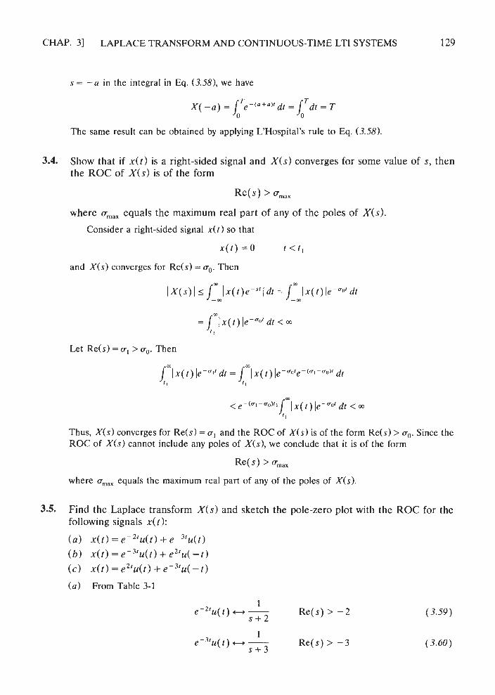
3.4. Show that if x ( t ) is a right-sided signal and X(s) converges for some value of s , then the R O C of X ( s ) is of the form

where amax equals the maximum real part of any of the poles of X ( s ) .

Consider a right-sided signal x(t) so that

and X(s) converges for Re(s) = a,. Then

Thus, X(s) converges for Re(s) =a, and the ROC of X(s) is of the form Re($) > a ( , . Since the ROC of X(s) cannot include any poles of X(s), we conclude that it is of the form

Re( s > ~ m a x

where a,,,,, equals the maximum real part of any of the poles of X(s).

3.5. Find the Laplace transform X ( s ) and sketch the pole-zero plot with the ROC for the following signals x( t ):

( a ) x ( t ) = e -"u( t ) + e P 3 ' u ( t ) ( b ) x ( t ) = e -"u( t ) + e 2 ' u ( - t ) (c) x ( t ) = e2 'u( t ) + e - 3 ' u ( - t )

(a) From Table 3-1


(b )

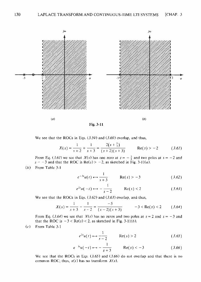
Fig. 3-1 1

We see that the ROCs in Eqs. (3.59) and (3.60) overlap, and thus,

From Eq. (3.61) we see that X(s) has one zero at s = - 5 and two poles at s = - 2 and s = - 3 and that the ROC is Re(s) > - 2, as sketched in Fig. 3-1 l(a).

(b) From Table 3-1

We see that the ROCs in Eqs. (3.62) and (3.63) overlap, and thus,

From Eq. (3.64) we see that X(s) has no zeros and two poles at s = 2 and s = -3 and that the ROC is - 3 < Re(s) < 2, as sketched in Fig. 3-1 l(b).

(c) From Table 3-1

1 e - 3 r ~ ( - t ) - - - Re(s) < - 3 (3.66)

s + 3

We see that the ROCs in Eqs. (3.65) and (3.66) do not overlap and that there is no common ROC; thus, x(t) has no transform X(s).


3.6. Let

Find X(s) and sketch the zero-pole plot and the ROC for a > 0 and a < 0.

The signal x ( t ) is sketched in Figs. 3-12(a) and ( b ) for both a > 0 and a < 0. Since x ( t ) is a two-sided signal, we can express it as

x ( t ) = e - " u ( t ) + e a ' u ( - r ) ( 3 . 6 7 )

Note that x ( t ) is continuous at t = 0 and x(O-) =x(O) =x (O+) = 1 . From Table 3-1

1 earu( - t ) H - - R e ( s ) < a ( 3 . 6 9 )

s - a

(c )

Fig. 3-12


If a > 0, we see that the ROCs in Eqs. (3.68) and (3.69) overlap, and thus,

1 1 - 2a x ( s ) = - - - = - -a < Re(s) < a s + a s - a s Z - a Z

From Eq. (3.70) we see that X ( s ) has no zeros and two poles at s = a and s = -a and that the ROC is -a < Re(s) < a , as sketched in Fig. 3-12(c). If a < 0, we see that the ROCs in Eqs. (3.68) and (3.69) do not overlap and that there is no common ROC; thus, X ( I ) has no transform X(s) .

PROPERTIES OF THE LAPLACE TRANSFORM

3.7. Verify the time-shifting property (3.161, that is,

x ( t - t o ) H e - " o X ( S ) R 1 = R

By definition (3 .3)

By the change of variables T = t - I , we obtain

with the same ROC as for X ( s ) itself. Hence,

where R and R' are the ROCs before and after the time-shift operation.

3.8. Verify the time-scaling property (3.181, that is,

By definition (3 .3)

By the change of variables 7 = a t with a > 0, we have

I w

( x a ) = - x(r)e-('/")'dr = - X - a -, a ( ) R P = a R

Note that because of the scaling s / a in the transform, the ROC of X ( s / a ) is aR. With a < 0, we have

CHAP. 31 LAF'LACE TRANSFORM AND CONTINUOUS-TIME LTI SYSTEMS 133

Thus, combining the two results for a > 0 and a < 0, we can write these relationships as

3.9. Find the Laplace transform and the associated ROC for each of the following signals:

( a ) x ( t ) = S(t - t o )

( b ) x ( t ) = u ( t - t o )

(c ) ~ ( t ) = e - " [ u ( t ) - u ( t - 5 ) ] ffi

( d l x ( t ) = S( t - k T ) k=O

( e ) x ( t ) = S(at + b) , a , b real constants

( a ) Using Eqs. (3.13) and (3.161, we obtain

S ( I - I,,) H e-s'fl all s

( b ) Using Eqs. (3.14) and (3.16), we obtain

( c ) Rewriting x ( l ) as

Then, from Table 3-1 and using Eq. (3.161, we obtain

( d ) Using Eqs. (3.71) and (1.99), we obtain

m m

~ ( s ) = C e-.~'T= C (e-sT)li = 1

1 - e s T k=O k -0

( e ) Let

f (0 = s ( a t ) Then from Eqs. (3.13) and (3.18) we have

1 f ( t ) = S(a1) - F ( s ) = -

la l

Re(s) > 0 (3.73)

all s

Now

Using Eqs. (3.16) and (3.741, we obtain

1 X ( s ) = e s b / a ~ ( S ) = -esh/" all s

la l


3.10. Verify the time differentiation property (3.20), that is,

From Eq. (3.24) the inverse Laplace transform is given by

Differentiating both sides of the above expression with respect to t, we obtain

Comparing Eq. (3 .77 ) with Eq. (3.76), we conclude that h ( t ) / d t is the inverse Laplace transform of sX(s). Thus,

Note that the associated ROC is unchanged unless

3.11. Verify the differentiation in s property (3.21),

R ' 3 R

a pole-zero cancellation exists at s = 0.

that is,

From definition (3 .3) - IIj

Differentiating both sides of the above expression with respect to s , we have

Thus, we conclude that

3.12. Verify the integration property (3.22), that is,

Let

Then


Applying the differentiation property (3.20), we obtain

X(s) =sF(s)

Thus,

The form of the ROC R' follows from the possible introduction of an additional pole at s = 0 by the multiplying by l/s.

Using the various Laplace transform properties, derive the Laplace transforms of the following signals from the Laplace transform of u(t).

( a ) 6(t) ( b ) 6'(t)

(c) tu(t) ( d ) e-"'u(t)

(e) te-"'u(t) (f) coso,tu(t)

(g) e-"'cos w,tu(t)

(a) From Eq. (3.14)we have

1 u(t) H - for Re( s) > 0

S

From Eq. ( 1.30) we have

Thus, using the time-differentiation property (3.20), we obtain

1 S(t) HS- = 1 all s

S

( b ) Again applying the time-differentiation property (3.20) to the result from part (a), we obtain

a'(!) H S all s ( 3.78)

(c) Using the differentiation in s property (3.211, we obtain

(dl Using the shifting in the s-domain property (3.17), we have

1 e-a'u(t) w - Re(s) > -a

s + a

(el From the result from part (c) and using the differentiation in s property (3.21), we obtain

(f) From Euler's formula we can write


Using the linearity property (3.15) and the shifting in the s-domain property (3.17), we obtain

( g ) Applying the shifting in the s-domain property (3.17) to the result from part (f), we obtain

3.14. Verify the convolution property (3.23), that is,

m

y ( t ) = x , ( t ) * x2( t ) = j x , ( r )x2 ( t - r ) d r - m

Then, by definition (3.3)

Noting that the bracketed term in the last expression is the Laplace transform of the shifted signal x2(t - 71, by Eq. (3.16) we have

with an ROC that contains the intersection of the ROC of X,(s) and X2(s). If a zero of one transform cancels a pole of the other, the ROC of Y(s) may be larger. Thus, we conclude that

3.15. Using the convolution property (3.23), verify Eq. (3.22), that is,

We can write [Eq. (2.601, Prob. 2.21

From Eq. (3.14)


and thus, from the convolution property (3.23) we obtain

1 x ( t ) * ~ ( t ) - -X(S)

5

with the ROC that includes the intersection of the ROC of X(s) and the ROC of the Laplace transform of u( t 1. Thus,

INVERSE LAPLACE TRANSFORM

3.16. Find the inverse Laplace transform of the following X(s): 1

( a ) X(s> = - , Re(s) > - 1 s + l

1 (b) X ( s ) = - , Re(s) < - 1

s + l S

( c ) X(s) = - , Re(s) > 0 s 2 + 4

s + l (d l X(s) = , Re(s) > - 1

( s + 1 ) '+4

(a) From Table 3-1 we obtain

( b ) From Table 3-1 we obtain

~ ( t ) = -e-'u(-t)

( c ) From Table 3-1 we obtain

x( t ) = cos2tu(t)

( d ) From Table 3-1 we obtain

~ ( t ) = e-'cos2tu(t)

3.17. Find the inverse Laplace transform of the following X(s):


Expanding by partial fractions, we have

Using Eq. (3.30), we obtain

Hence,

(a) The ROC of X(s) is Re(s) > - 1. Thus, x(t) is a right-sided signal and from Table 3-1 we obtain

x ( t ) = eP'u(t) + e - 3 ' ~ ( t ) = (e - ' + e - 3 ' ) ~ ( t )

( b ) The ROC of X(s) is Re(s) < -3. Thus, x( t) is a left-sided signal and from Table 3-1 we obtain

x ( t ) = -e - 'u ( - t ) - eC3'u( -1) = - ( e - ' +e-3 ' )u( -1)

(c) The ROC of X(s) is - 3 < Re(s) < - 1. Thus, x(t) is a double-sided signal and from Table 3-1 we obtain

3.18. Find the inverse Laplace transform of

We can write

Then

where


Thus,

The ROC of X(s) is Re(s) > 0. Thus, x ( t ) is a right-sided signal and from Table 3-1 we obtain

into the above expression, after simple computations we obtain

Alternate Solution:

We can write X(s) as

As before, by Eq. (3.30) we obtain

Then we have

Thus,

Then from Table 3-1 we obtain


We see that X(s) has one simple pole at s = - 3 and one multiple pole at s = -5 with multiplicity 2. Then by Eqs. (3.29) and (3.31) we have


By Eqs. (3.30) and (3.32) we have

Hence,

The ROC of X(s) is R d s ) > -3. Thus, x(t) is a right-sided signal and from Table 3-1 we obtain

Note that there is a simpler way of finding A , without resorting to differentiation. This is shown as follows: First find c , and A, according to the regular procedure. Then substituting the values of c , and A, into Eq. (3.84), we obtain

Setting s = 0 on both sides of the above expression, we have

from which we obtain A , =

3.20. Find the inverse Laplace transform of the following X(s):

2 s + 1 ( a ) X(s) = - , Re(s) > -2

s + 2

s3 + 2s' + 6 ( c ) X(S) = , Re(s) > 0

sz + 3s 2s + 1 2(s + 2) - 3

- 3

( a ) X ( s ) = - - = 2 - - s + 2 s + 2 s + 2

Since the ROC of X(s) is Re(s) > -2, x ( t ) is a right-sided signal and from Table 3-1 we obtain

( b ) Performing long division, we have

Let

where

Hence,

The ROC of X(s) is Re(s) > - 1. Thus, x ( r ) is a right-sided signal and from Table 3-1 we obtain

(c) Proceeding similarly, we obtain

Let

where

Hence,

The ROC of X(s) is Re(s) > 0. Thus, x(t) is a right-sided signal and from Table 3-1 and Eq. (3.78) we obtain

Note that all X(s) in this problem are improper fractions and that x(t) contains S(t) or its derivatives.



2 + 2se-" + 4eP4' X ( s ) = Re(s) > - 1

s2 + 4s + 3

We see that X ( s ) is a sum

where

2 2 s 4

X I ( $ ) = s 2 + 4s + 3 X 2 ( s ) = s t + 4s + 3 X A s ) = s 2 + 4s + 3

If

x l ( f ) - X d s ) x 2 ( t ) # X Z ( S ) ~ 3 ( f - X 3 ( s )

then by the linearity property (3 .15) and the time-shifting property (3 .16) we obtain

~ ( t ) = x l ( t ) + x 2 ( t - 2 ) + x 3 ( t - 4 ) ( 3 . 8 5 )

Next, using partial-fraction expansions and from Table 3-1, we obtain

3.22. Using the differentiation in s property (3.211, find the inverse Laplace transform of

We have

and from Eq. (3.9) we have

1 e - " u ( t ) o - R e ( s ) > - a

s + a

Thus, using the differentiation in s property (3.21), we obtain

X ( I ) = t e -" 'u( t )


SYSTEM FUNCTION

3.23. Find the system function H(s) and the impulse response h ( t ) of the RC circuit in Fig. 1-32 (Prob. 1.32).

( a ) Let

In this case, the RC circuit is described by [Eq. (1.105)]

Taking the Laplace transform of the above equation, we obtain

Hence, by Eq. (3.37) the system function H(s) is

Since the system is causal, taking the inverse Laplace transform of H(s), the impulse response h(t ) is

( b ) Let

In this case, the RC circuit is described by [Eq. (1.107)l

Taking the Laplace transform of the above equation, we have

1 or (s + &)Y(S) = Rsx(s )

Hence, the system function H(s) is


In this case, the system function H(s) is an improper fraction and can be rewritten as

Since the system is causal, taking the inverse Laplace transform of H(s), the impulse response h(t ) is

Note that we obtained different system functions depending on the different sets of input and output.

3.24. Using the Laplace transform, redo Prob. 2.5.

From Prob. 2.5 we have

h ( t ) = e-"'u(t) ~ ( t ) =ea 'u( - t ) a>O

Using Table 3-1, we have

1 H ( s ) = - Re(s) > -a

s + a

1 X(s ) = - - Re(s) < a

s - a

Thus,

and from Table 3-1 (or Prob. 3.6) the output is

which is the same as Eq. (2.67).

3.25. The output y ( t ) of a continuous-time LTI system is found to be 2e-3 'u( t) when the input x ( t is u( t ).

(a) Find the impulse response h ( t ) of the system. (6) Find the output y ( t ) when the input x ( t ) is e-'u(f).

( a ) x(f) = u(t), y(t) = 2e-3'u(t)

Taking the Laplace transforms of x( t) and we obtain



Rewriting H(s) as

and taking the inverse Laplace transform of H(s), we have

Note that h ( t ) is equal to the derivative of 2 e - " d l ) which is the step response s(r) of the system [see Eq. (2.1311.

I x ( t ) = e - ' d t ) ++ - Re(s)> - 1

s + l

Thus,

Using partial-fraction expansions, we get

Taking the inverse Laplace transform of Y(s), we obtain

y ( t ) = ( - e - ' + 3 e - " ) u ( r )

3.26. If a continuous-time LTI system is BIBO stable, then show that the ROC of its system function H ( s ) must contain the imaginary axis, that is, s = jo.

A continuous-time LTI system is BIBO stable if and only if its impulse response h ( t ) is absolutely integrable, that is [Eq. (2.2111,

By Eq. (3.3)

Let s = jw. Then

Therefore, we see that if the system is stable, then H(s) converges for s = jo. That is, for a stable continuous-time LTI system, the ROC of H(s) must contain the imaginary axis s = jw .


3.27. Using the Laplace transfer, redo Prob. 2.14.

( a ) Using Eqs. ( 3 . 3 6 ) and ( 3 . 4 0 , we have

Y ( s ) = X ( s ) H , ( s ) H , ( s ) = X ( s ) H ( s )

where H ( s ) = H , ( s ) H , ( s ) is the system function of the overall system. Now from Table 3-1 we have

Hence,

Taking the inverse Laplace transfer of H ( s ) , we get

h ( t ) = 2 ( e p ' - e - 2 ' ) u ( t )

(b) Since the ROC of H ( s ) , Re(s) > - 1, contains the jo-axis, the overall system is stable.


The system is described by

Taking the Laplace transform of the above equation, we obtain

s Y ( s ) + a Y ( s ) = X ( s ) or ( s + a ) Y ( s ) = X ( s )

Hence, the system function H ( s ) is

Assuming the system is causal and taking the inverse Laplace transform of H(s ) , the impulse response h ( t ) is

h ( t ) = e - " ' u ( t )

which is the same as Eq. (2.124).


The system is described by

y f ( t ) + 2 y ( t ) = x ( t ) + x l ( t )

Taking the Laplace transform of the above equation, we get

s Y ( s ) + 2 Y ( s ) = X ( s ) + s X ( s )

or ( s + 2 ) Y ( s ) = ( s + l ) X ( s )



Assuming the system is causal and taking the inverse Laplace transform of H(s), the impulse response h(t ) is

3.30. Consider a continuous-time LTI system for which the input x ( t ) and output y ( t ) are related by

~ " ( 1 ) + y l ( t ) - 2 y ( t ) = x ( t ) (3.86)

( a ) Find the system function H(s) .

( b ) Determine the impulse response h ( t ) for each of the following three cases: (i) the system is causal, (ii) the system is stable, (iii) the system is neither causal nor stable.

( a ) Taking the Laplace transform of Eq. (3.86), we have

s 2 ~ ( s ) + sY(s) - 2Y(s) = X(s )

or ( s 2 + s - ~ ) Y ( s ) = X ( s )


( b ) Using partial-fraction expansions, we get

(i) If the system is causal, then h(t) is causal (that is, a right-sided signal) and the ROC of H(s) is Re(s) > 1. Then from Table 3-1 we get

(ii) If the system is stable, then the ROC of H(s) must contain the jo-axis. Conse- quently the ROC of H(s) is - 2 < Re(s) < 1. Thus, h(t) is two-sided and from Table 3-1 we get

(iii) If the system is neither causal nor stable, then the ROC of H(s) is Re(s) < -2. Then h(r) is noncausal (that is, a left-sided signal) and from Table 3-1 we get

331. The feedback interconnection of two causal subsystems with system functions F ( s ) and G ( s ) is depicted in Fig. 3-13. Find the overall system function H ( s ) for this feedback system.

148

Let


- Fig. 3-13 Feedback system.

Then,

Y ( s ) = E ( s ) F ( s ) (3 .87)

R ( s ) = Y ( s ) G ( s ) (3 .88)

Since

e ( t ) = x ( t ) + r ( t )

we have

E ( s ) = X ( s ) + R ( s ) (3 .89)

Substituting Eq. (3.88) into Eq. (3.89) and then substituting the result into Eq. (3.87), we obtain

Y ( s ) = [ X ( s ) + Y ( s ) G ( s ) l F ( s ) or [ l - ~ ( s ) G ( s ) ] ~ ( s ) = F ( s ) X ( s ) Thus, the overall system function is

UNILATERAL LAPLACE TRANSFORM

3.32. Verify Eqs. (3 .44) and (3 .45) , that is,

d-41) ( a ) - H s X I ( s ) - x ( O - )

dl

( a ) Using Eq. (3.43) and integrating by parts, we obtain

Thus, we have


(b) Applying the above property to signal xt(t) = du(t)/dt, we obtain

Note that Eq. (3.46) can be obtained by continued application of the above procedure.

3.33. Verify Eqs. (3.47) and (3.481, that is, 1

( a ) L-X(T) d~ ++ - X , ( S ) S

(a) Let

Then

Now if

dl) ++G,(s)

then by Eq. (3.44)

X1(s) =sG1(s) -g(O-) =sGI(s)

Thus,

(b) We can write

Note that the first term on the right-hand side is a constant. Thus, taking the unilateral Laplace transform of the above equation and using Eq. (3.47), we get

3.34. (a ) Show that the bilateral Laplace transform of x ( t ) can be computed from two unilateral Laplace transforms.

(b) Using the result obtained in part (a ) , find the bilateral Laplace transform of e-21rl.


( a ) The bilateral Laplace transform of x ( t ) defined in Eq. (3.3) can be expressed as

Now / : x ( t ) e p " dl = X , ( s ) R e ( s ) > o+ (3 .92)

Next. let

ffi

Then ~ , ~ x ( - ~ ) e " d r = / ~ ( - r ) e - ' ~ ' ~ ' d t = X ; ( - s ) R e ( s ) < o- (3 .94 ) 0 -

Thus, substituting Eqs. (3.92) and (-3.94) into Eq. (3.91), we obtain

X ( s ) = X , ( s ) + X , ( - s ) a+< Re(s) <a- (3 .95 )

( b ) X ( t ) = e-21'I

( 1 ) x(t = e-2' for t > 0, which gives

(2) x(t ) = e2' for t < 0. Then x ( - t ) = e-2' for t > 0, which gives

Thus,

(3 ) According to Eq. (3.95), we have

which is equal to Eq. (3.701, with a = 2, in Prob. 3.6.

3.35. Show that

( a ) ~ ( 0 ' ) = lim s X , ( s ) ( 3 . 9 7 ) s-m

( b ) lim x ( t ) = lirn sX,(s ) t += s -0

( 3 . 9 8 )

Equation (3 .97 ) is called the initial value theorem, while Eq. (3.98) is called the final calue theorem for the unilateral Laplace transform.


( a ) Using Eq. (3.441, we have

m k ( ' ) e-" SX,(S) -x(o-) = / - 0- dt

W t ) = / O ' d ' o e - s ' d t +cT e -" dt 0- dt

a e-s t dt = x ( t ) E ? + / - o+ dt

- W f ) e-s,dt =x(O+) -x(o-) + / - o+ dt

Thus,

and lirn sX,(s) =x(O+) + 5-07

since lim, ,, e-" = 0.

( b ) Again using Eq. (3.441, we have

a & ( t ) lirn [sX,(s) - x(0-)] = 1im / - ePS' dt s-o s-o 0- dt

lirn e-"'

= lirn x(t ) - ~ ( 0 ~ ) t - r m

Since lirn [sX,(s) -x(0-)] = lim [sx,(s)] -x(O-) s-ro s-ro

we conclude that

limx(t) = lirnsX,(s) t--t- s-ro

3.36. The unilateral Laplace transform is sometimes defined as

with O+ as the lower limit. (This definition is sometimes referred to as the 0' definition.)

( a ) Show that


( b ) Show that

( a ) Let x ( t ) have unilateral Laplace transform X,?(s). Using Eq. (3.99) and integrating by parts, we obtain

Thus, we have

( b ) By definition (3.99) Oe OC

P + { u ( t ) ) = ,/ u ( t ) e - " d t = ,/ e-"dt 0' 0 '

1 R e ( s ) > 0

From Eq. (1.30) we have

Taking the 0' unilateral Laplace transform of Eq. (3.103) and using Eq. (3.100), we obtain

This is consistent with Eq. (1.21); that is,

Note that taking the 0 unilateral Laplace transform of Eq. (3.103) and using Eq. (3.44), we obtain

APPLICATION OF UNILATERAL LAPLACE TRANSFORM

337. Using the unilateral Laplace transform, redo Prob. 2.20. The system is described by

~ ' ( t ) + a y ( t ) = x ( l )

with y(0) = yo and x(t = ~ e - ~ ' u ( t 1.


Assume that y(0) = y(0-1. Let

~ ( t ) -Y,(s)

Then from Eq. (3.44)

y l ( t ) -sY,(s) -y(O-) =sY,(s) - Y o

From Table 3-1 we have

K x ( t ) -X, (S) = - R e ( s ) > -b

s + b

Taking the unilateral Laplace transform of Eq. (3.1041, we obtain

or

Thus,

+ K Y1(s) = -

s + a ( s + a ) ( s + b )

Using partial-fraction expansions, we obtain

Taking the inverse Laplace transform of Y,(s), we obtain

K y ( t ) =

yoe-"+ - ( e - b r - e - a : ) [ a - b

which is the same as Eq. (2.107). Noting that y(O+) = y(0) = y(0-) = yo, we write y( t ) as

K y ( t ) = y0e-O1 + - (e-br - e - a ' ) t 2 0

a - b

3.38. Solve the second-order linear differential equation

y " ( t ) + 5 y 1 ( t ) + 6 y ( t ) = x ( t )

with the initial conditions y(0) = 2, yl(0) = 1, and x ( t ) = e P ' u ( t ) .

Assume that y(0) = y(0-) and yl(0) = yl(O-). Let

~ ( t ) -Y,(s)

Then from Eqs. (3.44) and (3.45)

y l ( t ) -sY,(s) - y ( 0 - ) =sY , ( s ) - 2

y N ( t ) - s2Y1(s) - sy(0-) - y l ( O - ) = s 2 Y J s ) - 2s - I

From Table 3-1 we have


Taking the unilateral Laplace transform of Eq. (3.105), we obtain

Thus,

Using partial-fraction expansions, we obtain

Taking the inverse Laplace transform of Yl(s) , we have

Notice that y(O+) = 2 = y(O) and y'(O+) = 1 = yl(0); and we can write y ( f ) as

3.39. Consider the RC circuit shown in Fig. 3-14(a). T h e switch is closed at t = 0 . Assume that there is an initial voltage on the capacitor and uC(Om) = u,,.

( a ) Find the current i ( t ) .

( 6 ) Find the voltage across the capacitor uc( t ) .

vc (0- )=v,

( a ) (b)

Fig. 3-14 RC circuit.

( a ) With the switching action, the circuit shown in Fig. 3-14(a) can be represented by the circuit shown in Fig. 3-14(b) with i.f,(t) = Vu(t). When the current i ( t ) is the output and the input is r,(t), the differential equation governing the circuit is

1 Ri( t ) + -1' i ( r ) d~ = c s ( t ) (3.106)

C -, Taking the unilateral Laplace transform of Eq. (3.106) and using Eq. (3.481, we obtain


1 I Now ( t ) = - i ( r ) d r

C -,

and

Hence, Eq. (3.107) reduces to

Solving for I(s) , we obtain

v-0, 1 v - u , 1 I ( s ) = - =-

s R + 1/Cs R s + l /RC

Taking the inverse Laplace transform of I(s) , we get

( b ) When u,(r) is the output and the input is u,(t), the differential equation governing the circuit is

Taking the unilateral Laplace transform of Eq. (3.108) and using Eq. (3.441, we obtain

Solving for V,(s), we have

v 1 + uo Vc ( s ) = -

R C s ( s + l / R C ) s + l / R C

Taking the inverse Laplace transform of I/,(s), we obtain

u c ( t ) = V [ 1 - e - t / R C ] u ( t ) + ~ , e - ' / ~ ~ u ( t )

Note that uc(O+) = u, = u,(O-). Thus, we write uc(t) as

u c ( t ) = V(1 -e-'IRC) + ~ ~ e - ' / ~ ~ t r O

3.40. Using the transform network technique, redo Prob. 3.39.

( a ) Using Fig. 3-10, the transform network corresponding to Fig. 3-14 is constructed as shown in Fig. 3-15.


Fig. 3-15 Transform circuit,

Writing the voltage law for the loop, we get

Solving for I(s), we have

v - u , 1 v - u , 1 I ( s ) = - - --

s R + 1/Cs R s + l /RC

Taking the inverse Laplace transform of I(s) , we obtain

( b ) From Fig.3.15 we have

Substituting I (s ) obtained in part (a) into the above equation, we get

Taking the inverse Laplace transform of V,(s), we have

3.41. In the circuit in Fig. 3-16(a) the switch is in the closed position for a long time before it is opened at t = 0. Find the inductor current i(t) for t 2 0.

When the switch is in the closed position for a long time, the capacitor voltage is charged to 10 V and there is no current flowing in the capacitor. The inductor behaves as a short circuit, and the inductor current is = 2 A.

Thus, when the switch is open, we have i (O-)= 2 and u,(O-) = 10; the input voltage is 10 V, and therefore it can be represented as lOu(t). Next, using Fig. 3-10, we construct the transform circuit as shown in Fig. 3-16(b).


(b)

Fig. 3-16

From Fig. 3-16(b) the loop equation can be written as

or

Hence,

Taking the inverse Laplace transform of I(s), we obtain

Note that i(O+) = 2 = i(0-); that is, there is no discontinuity in the inductor current before and after the switch is opened. Thus, we have

3.42. Consider the circuit shown in Fig. 3-17(a). The two switches are closed simultaneously at t = 0. The voltages on capacitors C, and C, before the switches are closed are 1 and 2 V, respectively.

(a) Find the currents i , ( t ) and i,(t). ( b ) Find the voltages across the capacitors at t = 0'

( a ) From the given initial conditions, we have

uCl(O-) = 1 V and L!=~(O-) = 2 V

Thus, using Fig. 3-10, we construct a transform circuit as shown in Fig. 3-17(b). From


(b ) Fig. 3-17

Fig. 3-17(b) the loop equations can be written directly as

Solving for I ,(s) and I,(s) yields

Taking the inverse Laplace transforms of I , ( s ) and 12(s), we get

i l ( t ) = 6 ( t ) + i e - ' l 4 u ( t )

i 2 ( t ) = 6 ( t ) - f e - ' / 4 ~ ( t )

( b ) From Fig. 3-17(b) we have

Substituting I,(s) and 12(s) obtained in part ( a ) into the above expressions, we get


Then, using the initial value theorem (3.971, we have

s + l v , , ( O + ) = lim sVcl(s) = lim --7 + 1 = 1 + 1 = 2 V

s 4 m s - r m S + a

I S - 7 ucJO+) = lim sVC-(s) = lim ---7 + 2 = 1 + 2 = 3 V

s - + m s - + m S + , Note that ucl(O+)# u,1(0-) and ucz(O+)# ~ ~ $ 0 - ) . This is due to the existence of a capacitor loop in the circuit resulting in a sudden change in voltage across the capacitors. This step change in voltages will result in impulses in i , ( t ) and i2 ( t ) . Circuits having a capacitor loop or an inductor star connection are known as degener~t i~e circuits.

Supplementary Problems

3.43. Find the Laplace transform of the following x(t 1:

2 s ( c ) If a > 0 , X ( s ) = - - a < Re(s) < a. If a < 0, X ( s ) does not exist since X ( s ) does s z - ,2 '

not have an ROC. ( d ) Hint: x ( t ) = u ( t ) + u ( - t )

X ( s ) does not exist since X ( s ) does not have an ROC. ( e l Hint: x ( t ) = u ( t ) - u ( - t )

X ( s ) does not exist since X ( s ) does not have an ROC.

3.44. Find the Laplace transform of x ( t ) given by

t , _< t s t , x ( t ) =

0 otherwise

1 Am. X ( s ) = - [e-"I - e-"21, all s

S


3.45. Show that if X(I) is a left-sided signal and X(s) converges for some value of s, then the ROC of X(s) is of the form

where amin equals the minimum real part of any of the poles of X(s).

Hint: Proceed in a manner similar to Prob. 3.4.

3.46. Verify Eq. (3.21), that is,

Hint: Differentiate both sides of Eq. (3.3) with respect to s.

3.47. Show the following properties for the Laplace transform:

(a ) If x ( t ) is even, then X( -s) = X(s); that is, X(s) is also even.

(b) If ~ ( t ) isodd, then X(-s )= -X(s); that is, X(s) is alsoodd.

(c) If x ( t ) is odd, then there is a zero in X(s) at s = 0.

Hint:

( a ) Use Eqs. (1.2) and (3.17). (b) Use Eqs. (1.3) and (3.17).

(c ) Use the result from part (b) and Eq. (1.83~).

3.48. Find the Laplace transform of

x ( t ) = (e- 'cos21- Se-*')u(t) + :e2'u(-t)

s + l 5 1 1 Ans. X ( s ) = , - 1 < Re(s )<2

( ~ + 1 ) ~ + 4 S + 2 2 s - 2

3.49. Find the inverse Laplace transform of the following X(s);

1 ( b ) X(s) = -

s(s + l)? '

s + l (d) X(s) = , Re(s) > -2

s 2 + 4 s + 13


Am.

( a ) x ( r ) = ( 1 - e-' - t e - ' M t )

( b ) x ( t ) = - 4 - t ) -( l + t ) e - ' d t )

(c) ~ ( t ) = (- 1 + e-' + t e - ' I d - t )

( d ) x ( t ) = e - 2 ' ( ~ o s 3 t - f sin 3 t )u ( t )

( e l x ( t ) = at sin 2tu(t) ( f ) x ( t ) = ( - $e-2'+ Acos3t- t &sin3t )u( t )


Hint: Use Eq. (3.21) and Table 3-1.

3.51. Using the Laplace transform, show that

( a ) Use Eq. (3.21) and Table 3-1.

( b ) Use Eqs. (3.18) and (3.21) and Table 3-1.


Hint:

( a ) Find the system function H ( s ) by Eq. (3.32) and take the inverse Laplace transform of H(s) .

( 6 ) Find the ROC of H ( s ) and show that it does not contain the jo-axis.

3.53. Find the output y ( t ) of the continuous-time LTI system with

for the each of the following inputs:

(a) x ( t ) = e- 'u( t) ( b ) x ( t ) = e-'u(-t)

Ans.

( a ) y ( r ) = (e- ' -e-")u(t) ( b ) y ( t ) = e- 'u(- f )+e- 2 ' ~ ( t )

3.54. The step response of an continuous-time LTI system is given by (1 - e- ' )u( t) . For a certain unknown input x ( t ) , the output y ( t ) is observed to be (2 - 3e-' + e-3')u(r). Find the input x( t ) .


Fig. 3-18

Determine the overall system function H ( s ) for the system shown in Fig. 3-18.

Hint: Use the result from Prob. 3.31 to simplify the block diagram. S

Am. H ( s ) = s 3 + 3 s 2 + s - 2

If x ( t ) is a periodic function with fundamental period T, find the unilateral Laplace transform of x ( t ) .

Find the unilateral Laplace transforms of the periodic signals shown in Fig. 3-19.

Using the unilateral Laplace transform, find the solution of

y " ( t ) - y l ( t ) - 6 y ( t ) = e t

with the initial conditions y ( 0 ) = 1 and y ' (0 ) = 0 for t 2 0.

Am. y ( t ) = - ; e l + fe -2 '+ ;e3', t z O

Using the unilateral Laplace transform, solve the following simultaneous differential equations:

y l ( t ) + y ( t ) + x f ( r ) + x ( t ) = 1

y l ( t ) - y ( t ) - 2 x ( t ) = O

with x ( 0 ) = 0 and y ( 0 ) = 1 for t 1 0 .

Ans. x ( t ) = e-' - 1 , y ( t ) = 2 - e - ' , t r 0

Using the unilateral Laplace transform, solve the following integral equations:

A m . ( a ) y ( t ) =ea t , t 2 0 ; ( 6 ) y ( t ) = e 2 ' , t 2 0


(b) Fig. 3-19

3.61. Consider the RC circuit in Fig. 3-20. The switch is closed at t = 0 . The capacitor voltage before the switch closing is u,. Find the capacitor voltage for t 2 0.

Ans. u , ( t ) = ~ , e - ' / ~ ~ , 1 2 0

3.62. Consider the RC circuit in Fig. 3-21. The switch is closed at t = 0. Before the switch closing, the capacitor C , is charged to u, V and the capacitor C , is not charged.

( a ) Assuming c , = c , = c , find the current i ( t ) for t 2 0 . ( b ) Find the total energy E dissipated by the resistor R and show that E is independent of R

and is equal to half of the initial energy stored in C , .


1 64 LAPLACE TRANSFORM AND CONTINUOUS-TIME LTI SYSTEMS [CHAP. 3


(c) Assume that R = 0 and C , = C , = C . Find the current i ( r ) for I 2 0 and voltages u,1(0+) and uC2(0+).

schaum's outlines of signals & systems (ripped by sabbanji) · pdf filechap. 31...

Documents