school of economics university college cork working … · school of economics university college...
TRANSCRIPT

1
School of Economics
University College Cork
Working Paper Series
Controlling for Endogeneity in the Relationship between Life Satisfaction
and Employment Status
Working Paper 13-03
Edel Walsh & Rosemary Murphy
Abstract: This paper aims to examine if a simultaneous relationship exists between life
satisfaction and employment status. A sample of 2,576 Irish adults obtained from the
European Social Survey 5 is used to test this hypothesis. A two-stage probit least squares
technique estimates life satisfaction and employment status simultaneously and accounts for
the endogeneity present in the equations in the system. The findings suggest a bi-directional
relationship between life satisfaction and employment status that is, employment affects life
satisfaction but also being satisfied with life increases the predicted probability of being
employed. Furthermore, this paper finds that the effect of employment status on life
satisfaction (as well as the reverse direction effect) is underestimated if simultaneous
endogeneity is not accounted for.
Keywords: Life satisfaction, employment status, endogeneity, two-stage probit least squares,
European Social Survey
JEL classifications: I31, J21
Corresponding author contact details: Dr Edel Walsh, School of Economics, University
College Cork. [email protected]
*These Discussion Papers often represent preliminary or incomplete work, circulated to
encourage discussion and comments. Citation and use of such a paper should take account
of its provisional character. A revised version may be available directly from the author(s).
Further working papers are available at http://www.ucc.ie/en/economics

2
1. INTRODUCTION
The direction of the relationship between well-being and employment status has been
questioned in existing literature which suggests that the relationship may be hampered by
endogeneity, making employment status both a cause and a consequence of well-being
(Hamilton et al., 1997; Duarte et al., 2007; Cole et al., 2009). Studies agree that the
endogeneity may be caused by a simultaneous relationship between well-being and
employment status, that is, employment affects life satisfaction1 but also being satisfied with
life is a determinant for securing employment (Hamilton et al., 1997; Cole et al., 2009). If the
causal relationship between life satisfaction and employment status runs in both directions
any estimation without controlling for such simultaneous endogeneity would yield biased and
inconsistent estimates of the structural parameters. The aim of this paper is to estimate life
satisfaction and employment status simultaneously to account for the potential endogeneity of
these two variables.
Existing research is primarily focused on the effect of employment status on well-
being with most studies supporting the finding that unemployment has a large, negative effect
on well-being2 (Di Tella et al., 2001; Frey and Stutzer, 2000, 2002; Helliwell, 2003; Stutzer,
2004). The observed association between unemployment and well-being does, however, not
necessarily mean that unemployment causes poor well-being. The causality may also go in
the other direction, that is, well-being may be a factor in determining employment status.
Individuals who experience low levels of well-being may be more likely to become
unemployed, if for example, they are less productive at work or have high levels of
absenteeism due to poorer health (Paul and Moser, 2009). This simultaneous (or bi-
directional) relationship between well-being and employment status has received much less
attention in the existing literature.
In this paper the relationship between life satisfaction and employment status is
estimated using a sample of 2,576 Irish adults obtained from the European Social Survey 5
(ESS5). The main contribution of this paper is the estimation of life satisfaction and
1 Life satisfaction is a component of subjective well-being (Diener et al., 1999).
2 There are some exceptions to the finding of strong negative effect of unemployment (Graham and Pettinato,
2001; Smith, 2003), however this may be due to small numbers of unemployed in their data.

3
employment status simultaneously to control for the endogeneity of these two variables. A
unique aspect of this paper is that two additional measures of well-being (namely ‘happiness’
and ‘wellbeing’) are used to test the robustness of the results. In addition, the models are
estimated without controlling for endogeneity to allow for a comparison to be made with
models in which simultaneity is not accounted for. A number of other factors associated with
life satisfaction and employment status are also identified. A Two-Stage Probit Least Squares
(2SPLS) empirical methodology is used to control for the endogeneity in the life satisfaction-
employment status relationship.
The remainder of the paper is organised as follows. Section 2 presents a review of the
existing literature in the area. Section 3 outlines the data used and defines the main variables.
The econometric model is explained in Section 4. This is followed by a discussion of the
results obtained and a summary of the main conclusions in Section 5. Section 6 concludes.
2. LITERATURE REVIEW
The relationship between well-being and employment status has undergone extensive
investigation in existing literature, focusing mainly on the effect of employment status on
well-being (Blanchflower, 1996; Brereton et al., 2008; Clark and Oswald, 1994; Frey and
Stutzer, 1999; Winkelmann and Winkelmann, 1998). These and other studies find that the
relationship tends to run in the direction from employment status to well-being, specifically
that unemployment leads to lower levels of well-being and employment leads to higher levels
of well-being, up to a certain point (Korpi, 1997; Di Tella et al., 2002; Frey and Stutzer,
2000; Helliwell, 2003; Stutzer, 2004). However, more recently the direction of the
relationship between employment status and well-being has been questioned and research
suggests that the relationship goes in both directions (simultaneous endogeneity), that is,
employment status affects well-being but also having high levels of well-being determines
the probability of being employed (Hamilton et al., 1997; Cole et al., 2009). Research
suggests that people with low levels of well-being may have a higher probability of losing
their jobs and furthermore, when unemployed, exhibit negative traits which hinder their
chances of finding new employment (Toppen, 1971; Winefield, 1995; Mastekaasa, 1996). In
contrast high levels of well-being, and in particular self-esteem, can improve an individual’s

4
chances of employment. Winefield and Tiggemann (1985), Caplan et al., (1989) and Waters
and Moore (2002) find that high levels of self-esteem are associated with finding
employment.
Paul and Moser (2009) propose that an individual’s unemployment is a consequence
and not a cause of poor well-being. They find that the effect could be the result of several
processes. Firstly, poor well-being might reduce an employee’s performance at work or might
increase absenteeism due to illness. Issues such as this might in turn increase the likelihood of
dismissal (Mastekaasa, 1996; Paul and Moser, 2009). Hesselius (2007) finds that an increase
in the number of sick days in addition to an increase in the duration of sick spells are
associated with a higher risk of unemployment. Secondly, distress may play a role with
regard to the job search process. An employer’s hiring decision is likely to be influenced by
the applicant’s impression on management, a variable that may be influenced by well-being
(Paul and Moser, 2009). Thirdly, poor well-being may be expected to reduce the effort and
the efficiency of an individual’s job search which in turn reduces the probability of re-
employment (Paul and Moser, 2009; Cole et al., 2009). Similarly, Crossley and Stanton
(2005) suggest that the distress resulting from unemployment has a negative relationship with
both interview and job-search success. These studies support the idea that well-being is a
significant factor in determining one’s employment status. However, controlling for
simultaneous endogeneity is a major empirical problem when estimating the effect of
employment on well-being (Gerdtham and Johannesson, 2003).
Few existing studies however, have estimated the relationship between well-being and
employment status while controlling for simultaneous endogeneity and, therefore, risk
reporting biased results. In Ireland, existing research (Whelan, 1992a, 1992b, 1994; Hannan
et al., 1997; Brereton et al., 2008) has estimated the effect of employment status on well-
being without controlling for endogeneity. Brereton et al., (2008) examine the relationship
between employment status and well-being in Ireland using data from 2001. The study
examines the welfare impacts of a number of employment status categories on life
satisfaction, including part-time employment, disconnection from the labour force and being
disabled, unable to work in Ireland. They find that being long-term unemployed, disabled and
unable to work or in part-time employment, have significant negative effects on life
5
satisfaction, particularly for Irish males. However, Brereton et al., (2008), while
acknowledging that it may be an issue, fail to control for the potential simultaneous
endogeneity in the relationship between life satisfaction and employment status. Furthermore,
their study may be less relevant in the context of the current economic climate in Ireland3.
Hannan et al., (1997) assume that the direction of causality is from unemployment to
psychological distress. Similarly, Whelan (1992a; 1992b; 1994) analysed the effect of
unemployment on psychological distress. These studies take psychological distress rather
than life satisfaction as a measure of well-being which makes it difficult to compare their
findings with much of the existing well-being literature. Neither Whelan (1992) nor Hannan
et al., (1997) controlled for simultaneous endogeneity in their research and assumed the
direction of causality was from unemployment to well-being (psychological distress).
Simultaneous endogeneity has been recognised as a significant problem in the
existing literature. It occurs when at least one of the explanatory variables is determined
along with the dependent variable (Wooldridge, 2002). The presence of endogeneity in a
model is a problem as it can seriously bias the independent effect of the endogenous
variables. The methods of estimating such a relationship have been widely discussed in the
statistical literature (Gujarati, 1995; Pindyck and Rubinfeld, 1991; Davidson and MacKinnon,
1993; Greene, 2000; Judge et al., 1985). The issue is that standard estimation methods, such
as Ordinary Least Squares (OLS), used to estimate models in the presence of simultaneous
endogeneity will result in biased and inconsistent estimates (Keshk, 2003). Endogeneity can
be controlled for by using empirical methodologies such as Indirect Least Squares (ILS) or
Two-Stage Least Squares (2SLS). For studies involving systems of equations where one
endogenous variable is continuous and the other endogenous variable is dichotomous, Two-
Stage Probit Least Squares (2SPLS) methodology should be used.
Some previous research attempted to control for endogeneity in the well-being-
employment status relationship using indirect methods or through two stage procedures.
Hamilton et al., (1997) apply a maximum likelihood, simultaneous equation generalized
3 Figures from the CSO (2013) signal the current unemployment rate in Ireland is 14 per cent. Brereton et al.,
(2008) utilise Irish data from 2001 when the unemployment rate was 4 per cent.
6
probit model to jointly estimate the determinants of an individual’s employment status and
their mental health in Canada. Duarte et al., (2007) use a simultaneous equation generalized
probit model but do not find support for a simultaneous relationship and conclude that the
relationship runs from well-being to employment. Using a two-stage least squares regression
technique on Australian data, Cole et al., (2009) tests the hypothesis of a simultaneous
relationship between employment status and well-being and find support for such a
relationship.
This paper attempts to control for the simultaneous endogeneity in the life
satisfaction-employment status relationship by estimating the system of equations via two-
stage probit least squares (2SPLS). The null hypothesis is that no simultaneous relationship
exists between life satisfaction and employment status. Using 2SPLS it is possible to
ascertain if life satisfaction is affecting employment status and employment status affecting
life satisfaction simultaneously.
3. DATA
The European Social Survey (ESS) is a biennial, cross-sectional survey of about 30
countries in Europe including Ireland. The initial sample, ESS1, was collected in 2002. The
ESS draws a different sample of individuals each time it is conducted. Respondents are
interviewed on a range of topics including their age, gender, educational status, employment
status and life satisfaction. The analysis in this paper is based on Irish data from the European
Social Survey 5 (ESS5) which was conducted in 2010. This dataset provides a random
sample of 2,576 Irish respondents. Within the ESS5 the following question on life
satisfaction is asked; ‘All things considered, how satisfied are you with your life as a whole
nowadays?’ Respondents are asked to rank their answer on an eleven-point scale ranging
from 0 “extremely dissatisfied” to 10 “extremely satisfied”. This elicits a measure for life
satisfaction and this measure is frequently used in economic studies on well-being
(Winkelmann and Winkelmann, 1998; Helliwell, 2003; Frey and Stutzer, 2005).

7
As well as life satisfaction, the ESS5 contains detailed information on a sample of
Irish respondents’ employment status. Life satisfaction and employment status are the
dependent (endogenous) variables in the system of equations estimated in Section 4. A
number of other personal and socio-economic characteristics namely age, gender, education,
disability status, area of residence (rural/urban) and marital status are also contained in the
ESS5. These are used as the independent (exogenous) variables in the model. Table 3.1
includes a detailed description and summary statistics of the endogenous and exogenous
variables used in this study. Due to the qualitative nature of most of the variables it was
necessary to create dummy variables, where a value of 1 or 0 indicates the presence or
absence of an attribute.
<Insert Table 3.1 about here>
<Insert Figure 3.1 about here>
Table 3.1 displays the means and standard deviations for the dependent and
independent variables used in this paper. Life satisfaction, which is measured on a 0-10 scale,
has a mean value of 6.455. The modal score is 8 with over 21% of respondents indicating this
as their life satisfaction score (Figure 3.1). Approximately 7% of respondents are ‘extremely
satisfied with life’ as indicated by a maximum score of 10 and 1% are ‘extremely dissatisfied
with life’ indicated by the lowest score of 0. Of those in the employment status category, 945
respondents reported being in paid employment and 393 reported being unemployed (either
actively seeking work or not actively seeking work). In the sample, the distribution of
respondents by gender was equitable and their ages ranged from 15 to 101 years, with the
mean age being 46 years approximately.
<Insert Table 3.2 about here>
Table 3.2 displays information pertaining to life satisfaction and employment status of
individuals in the sample. Almost 60% of unemployed respondents indicated a score of 5 or
lower on the 11-point life satisfaction scale. By contrast the proportion of employed
respondents with scores at the bottom of the life satisfaction scale was much lower. 27.7% of
the employed in the sample reported scores of 5 or lower on the life satisfaction scale. The
percentage of employed reporting a life satisfaction score of 7, 8, 9 or 10 is twice that of the
unemployed in each of these categories. Moreover, over 72% of those who have jobs reported

8
their life satisfaction to be 6 or higher whereas, only 40% of unemployed individuals rated
their life satisfaction as 6 or above.
4. Econometric Model
This paper uses a two-stage probit least squares (2SPLS) estimation method described
in Maddala (1983) for simultaneous equation models in which one of the endogenous
variables is continuous and the other endogenous variable is dichotomous. The method
estimates life satisfaction and employment status simultaneously and accounts for any
endogeneity in the equations in the system4.
Employment status, among other covariates, is assumed to be a function of life
satisfaction. Endogeneity is an issue because life satisfaction is also a function of
employment status. This paper addresses the endogeneity issue and estimates the following
simultaneous structural equations for life satisfaction (LS) and employment status (ES);
11
'
1211 εβγ +Χ+= ∗ESLS (1)
22
'
2122 εβγ +Χ+=∗ LSES (2)
where:
LS1 = continuous endogenous variable Life Satisfaction5
∗2ES = dichotomous endogenous variable, Employment Status
which is observed as a 1 if ∗2ES > 0, and a 0 otherwise
X1 = matrix of exogenous variables in (1)
X2 = matrix of exogenous variables in (2)
'
1β = vector of parameters in (1)
'
2β = vector of parameters in (2)
1γ = parameters of the endogenous variables in (1)
4 Using the cdsimeq command the statistical software package Stata ensures that all the necessary procedures for
obtaining consistent estimates for the coefficients, as well as their corrected standard errors are obtained. 5 Helliwell (2003) and Ferrer-i-Carbonell and Frijters, (2004) claim that it makes little difference if the life
satisfaction variable is treated as ordinal or cardinal.

9
2γ = parameters of the endogenous variables in (2)
1ε = error term of (1)
2ε = error term of (2)
The estimation follows the two-stage estimation process used in simultaneous equation
modelling as prescribed by Keshk (2003). In the first stage the following two equations (3
and 4) are fitted using all of the exogenous variables in equations (1) and (2) (Maddala,
1983),
1
'
11 ν+ΧΠ=LS (3)
2
'
22 ν+ΧΠ=∗∗ES (4)
where:
LS1 = life satisfaction
∗∗2ES = employment status
1Π , 2Π = vectors of parameters to be estimated
X = matrix of all the exogenous variables
v1, v2 = error terms
In estimating the first stage regressions equation (3) is estimated via OLS and equation (4) is
estimated via probit. A condition for simultaneous equation models is that there is at least one
independent variable that does not appear in the other equation (Cai and Kalb, 2006). This
paper includes a dummy variable for having a disability or health problem that hampers an
individual’s daily life6 in the life satisfaction equation and a dummy variable for marital
status in the employment status equation. The decision to use these variables is based on
existing literature (Hamilton et al., 1997; Duarte et al., 2007). From these reduced form
estimates the predicted values from each model are obtained for use in the second stage
(Maddala, 1983):
6 This is a physical rather than a psychological measure of the health status of the respondent.

10
111ˆ Χ∏=
∧
LS (5)
222ˆ Χ∏=
∗∗∧
ES (6)
where;
1
∧
LS = predicted value of Life Satisfaction
1∏̂ = vector of parameters
X1 = vector of exogenous variables used to estimate 1
∧
LS
∗∗∧
2ES = predicted value of Employment Status
1∏̂ = vector of parameters
X2 = vector of all exogenous variables used to estimate∗∗∧
2ES
In the second stage the original endogenous variables in equation (1) and equation (2) are
replaced by their respective predicted values in equations (5) and (6). In the second stage, the
following models are fitted:
111211 εβγ +Χ+=∗∗∧
ESLS (7)
222122 εβγ +Χ+=∧
∗∗ LSES (8)
where;
LS1 = life satisfaction
∗∗2ES = employment status
1γ = parameters of the endogenous variables in (7)
2γ = parameters of the endogenous variables in (8)
∗∗∧
2ES = predicted value of employment status in (7)
11
1
∧
LS = predicted value of life satisfaction in (8)
1β = vector of parameters in (7)
2β = vector of parameters in (8)
X1 = matrix of exogenous variables in (7)
X2 = matrix of exogenous variables in (8)
1ε = error term in (7)
2ε = error term in (8)
As before, equation (7) is estimated via OLS and equation (8) is estimated via probit.
The estimated standard errors for each model in the second stage (equations 7 and 8)
are based on ∗∗∧
2ES and 1
∧
LS and not on the appropriate ∗∗2ES and LS1 and so are incorrect
(Keshk, 2003). The correction needs to be implemented on the variance-covariance matrices
of equation (7) and (8) which are α1 and α2 respectively (Keshk, 2003). The asymptotic
covariance matrix can be derived by using a procedure similar to the one used by Amemiya
(1979). Given the estimable parameters in the model the following is defined according to
Maddala (1983):
),( '
121
'
1 βσγα = (9)
=
2
'
2
2
2'
2 ,σ
β
σ
γα
(10)
c = 121
2
1 2 σγσ − (11)
−
=
2
12
2
22
1
2
2 2σ
σ
σ
γσ
σ
γd
(12)
H = (П2, J1) (13)
G = (П1, J2) (14)
12
V0 = Var )ˆ( 2∏ (15)
In probit models 2σ is normalised to 1 and therefore the corrected variances of α1 and α2 are
obtained as follows:
V ( )1α̂ = c(H` X` XH)-1
+ (γ1 σ2)2(H` X` XH)
-1 H`X`V0X`XH(H`X`XH)
-1 (16)
V ( )2α̂ = (G` V0-1
G)-1
+ d(G` V0-1
G)-1
G` V0-1
(X`X)-1
V0-1
G(G` V0-1
G)-1 (17)
where;
2
1σ = variance of the residuals from (3)
V0 = variance-covariance matrix of (4)
J1 and J2 = matrices with ones and zeros such that XJ1 = X1 and
XJ2 = X2
According to Achen (1986) these corrected standard errors are superior to the uncorrected
standard errors. The procedure described above is carried out using the data analysis and
statistical software package Stata. The results from the equations (7) and (8) with corrected
standard errors, are discussed in Section 5.
5. RESULTS
The presence of simultaneous endogeneity in the model implies that in the life
satisfaction equation the coefficient on employment status would be significant and in the
employment equation the coefficient on life satisfaction would be significant (Cai and Kalb,
2006). To establish the correlation between life satisfaction and employment status the
equations are first estimated without controlling for endogeneity. This corresponds to
estimating equations (1) and (2) above by OLS and Probit respectively. The estimates
presented in the first column of Table 5.1 show that being employed increases life
satisfaction by 1.16 points on the life satisfaction scale7. Furthermore, the result is statistically
significant at the 1 per cent level in explaining life satisfaction. The second column shows
7 A full set of results for this estimation can be found in Table A1 in Appendix A.
13
that life satisfaction is also found to be statistically significant in explaining employment
status. The positive coefficient indicates that higher levels of life satisfaction increase the
predicted probability of being employed.
These results suggest that the relationship between life satisfaction and employment
status is bi-directional. As previously indicated, however, these OLS and probit estimates are
biased and inconsistent as life satisfaction and employment status are jointly determined in
the presence of simultaneous endogeneity. To address this simultaneity the equations are now
estimated by Two-Stage Probit Least Squares which controls for the endogeneity of life
satisfaction and employment status and produces unbiased and consistent estimates.
<Insert Table 5.1 about here>
5.1. Two Stage Probit Least Squares (2SPLS) Estimation Results
The 2SPLS estimation results for the life satisfaction equation and the employment
status equation are presented in Table 5.28. These results are estimated controlling for the
endogeneity of life satisfaction and employment status. The first column of Table 5.2
presents the estimated coefficients and their corrected standard errors for the life satisfaction
equation where life satisfaction (on a scale 0-10) is the dependent variable, while the second
column shows the estimations for employment status, where a binary variable for
employment status (0 unemployed, 1 employed) is the dependent variable.
<Insert Table 5.2 about here>
The results from the life satisfaction equation will be discussed first. The first
independent variable relates to the individual’s employment status. Employment is associated
8The data analysis and statistical software package Stata 11 was used to conduct the econometric analysis.

14
with a 1.5 point increase in life satisfaction and the result is statistically significant at the 1
per cent level. This is consistent with much of the existing literature. For example, Flatau et
al., (2000) find that the employed enjoy greater mental health and well-being than the
unemployed or part-time employed in Australia. In a study similar to this one however,
Duarte et al., (2007) find a positive but insignificant coefficient on the employment variable
in the well-being equation and conclude that the direction of the relationship runs from well-
being to employment status only. Using a simultaneous equation generalized probit model
Hamilton et al., (1997) find that the higher values of the latent index of employability are
associated with better health. The result here indicates that, other things being equal, higher
life satisfaction increases the probability of being employed.
The results show that there is no statistically significant relationship between
education and life satisfaction. There is a positive relationship between life satisfaction and
being 24 years of age or younger. This result is significant at the 1 per cent level. Being aged
between 25 and 34 is also positively correlated with life satisfaction and statistically
significant at the 5 per cent level. Being in the youngest age category (age ≤24) increases an
individual’s life satisfaction by 1.1 points on the 11 point life satisfaction scale, holding other
factors constant. If an individual is aged between 25 and 34 this increases their life
satisfaction by 0.43 points. All of the other age variables are insignificant. Using a
simultaneous equation model similar to the one used in this paper, Duarte et al., (2007) also
report insignificant coefficients on their age variables in the well-being equation.
With respect to gender, males are more satisfied with life than females. This is in
contrast to the literature which generally finds women are happier than men (Alesina et al.,
2004). However, the result here is significant at the 1 per cent level and suggests that being
male increases life satisfaction by about half a point on the scale. Living in a rural area in
Ireland also emerges significant and positive in the regression. The coefficient indicates that
if an individual is living in a rural area their life satisfaction increases by 0.378 points on the
life satisfaction scale compared to those living in an urban area, ceteris paribus. Earlier
research has found a strong correlation between measures of objective health status and life
satisfaction. The results here suggest that having a disability decreases life satisfaction by
0.52 points on the scale and this result is significant at the 10 per cent level. This finding is

15
consistent with the Australian study by Cole et al., (2009) who find that having a health
problem or disability has a significant and negative impact on well-being. Furthermore,
Duarte et al., (1994) find that being physically limited reduces well-being considerably.
The second column of results in Table 5.2 presents the results for the estimated
employment status equation (8) above. The coefficient for life satisfaction emerges positive
and significant suggesting that, all other things being equal, higher levels of life satisfaction
increase the predicted probability of being employed. Hamilton et al., (1997), Duarte et al.,
(2007) and Cole et al., (2009) all find that higher levels of well-being (or some other self-
assessed well-being/health variable) lead to an increased probability of participation in the
labour force in Canada and Australia.
Other significant variables in the employment status equation include education, age,
gender and marital status. As one would expect higher levels of education (post-secondary
and tertiary education) increase the probability of being employed. Most of the age categories
are insignificant in the employment status equation which is consistent with Hamilton et al.,
(1997). Exceptions here are that being less than 24 years of age is negatively associated with
the probability of being employed. Males have a lower probability of being employed than
women and this is highly statistically significant at the 1 per cent level. Finally, marriage is
correlated with having a job and this coefficient is significant at the 10 per cent level.
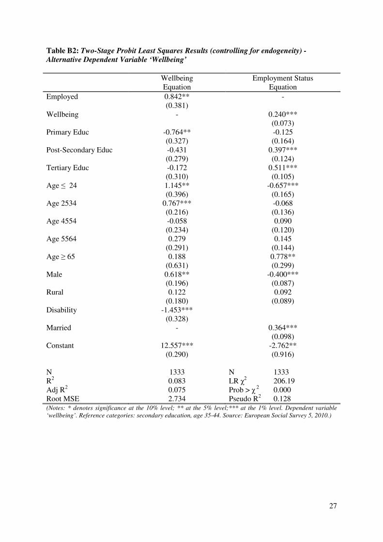
To test the robustness of the results the models were again estimated using 2SPLS
using two alternative measures for well-being. Instead of life satisfaction, alternative
dependent variables ‘happiness’ and ‘wellbeing’ were used to estimate the model. Similar to
the ‘life satisfaction’ variable ‘happiness’ is also measured on a scale from 0 to 10; where 0
indicates extreme unhappiness and 10 indicates extreme happiness. ‘Wellbeing’ is a variable
comprised of the following three questions; ‘I have felt cheerful and in good spirits’ ‘I have
felt calm and relaxed’ ‘I have felt active and vigorous’. Respondents answered; ‘All of the
time’, ‘Most of the time’, ‘More than half of the time’, ‘Less than half of the time’, ‘Some of
the time’, ‘At no time’. Each respondent was given a score ranging from 3 (lowest well-
being) to 18 (highest well-being). The results suggest that a bi-directional relationship exists

16
between well-being and employment status regardless of the measure of well-being used. The
results from these regressions are presented in Tables B1 and B2 in Appendix B.
Based on the results the null hypothesis of no simultaneous relationship between life
satisfaction and employment status is rejected. This paper suggests that a simultaneous
relationship exists in the model, where, employment has a positive and significant effect on
life satisfaction and life satisfaction has a positive and significant effect on employment
status. The finding corroborates existing research by Cole et al., (2009) who find a
significant, simultaneous relationship between labour market status and well-being in
Australia. Similarly, Hamilton et al., (1997) use mental health as a proxy for well-being and
find a simultaneous relationship between employment and mental health in Canada. The
results contribute to the existing body of literature on well-being in Ireland by establishing
the life satisfaction-employment status relationship simultaneously.
6. SUMMARY AND CONCLUSION
This paper has estimated the determinants of life satisfaction and employment status
in Ireland using 2010 data from the ESS5. A simple OLS estimation revealed that there is
indeed a positive and statistically significant correlation between life satisfaction and
employment in Ireland. However, OLS does not account for simultaneous endogeneity
present in a model. The main focus of this paper was to control for this simultaneous
relationship between life satisfaction and employment status. The results find support for a
simultaneous or bi-directional relationship and indicate that employment leads to higher
levels of life satisfaction and higher levels of life satisfaction increase the predicted
probability of being in employment. The results from the 2SPLS model indicate that the
relationship is seriously underestimated if endogeneity is not controlled for. Two alternative
well-being variables were used to test the robustness of the results and it was found that the
bi-directional relationship holds regardless of the measure of well-being used.
Since they do not account for endogeneity many of the existing well-being studies
may underestimate the importance of the relationship between life satisfaction and

17
employment status. This paper expands the analysis on well-being in Ireland by using two-
stage methods to control for endogeneity. In agreement with previous literature employment
is found to affect life satisfaction, and vice versa, but after controlling for endogeneity the
result is found to be even more important. Other results find that men are more satisfied with
their lives than women and that people living in rural areas have higher levels of life
satisfaction than people living in big cities. Age is another factor found to affect life
satisfaction with individuals less than 34 years of age more satisfied with life than middle
aged (35-44) individuals. Moreover, having a disability or serious health problem has a
negative and statistically significant effect on life satisfaction.
With respect to employment this paper finds that apart from life satisfaction
education, gender, age and marital status all affect the probability of being employed. Not
surprisingly, higher levels of education have a positive and significant effect on the predicted
probability of being employed. Furthermore, younger people have a significantly lower
chance of being in employment. Women and those who are married are also found to have a
higher probability of being in employment.
In conclusion, the main results from this paper find support for a simultaneous
relationship between life satisfaction and employment status using 2010 Irish data from the
ESS5. After controlling for simultaneous endogeneity, using a Two Stage Probit Least
Squares estimation technique, this research finds that employment leads to higher levels of
life satisfaction and higher levels of life satisfaction increase the predicted probability of
being employed. Much of the current literature has failed to correctly identify and control for
this simultaneous relationship and therefore report biased estimates. This paper suggests that
relationship between life satisfaction and employment may be underestimated in the current
literature which has failed to control for simultaneous endogeneity. Therefore, the results
from this paper shed new light on the extent of the relationship between these variables and
provide new information on the determinants of life satisfaction and employment status
which may prove useful for the government and other policy makers in Ireland and
elsewhere.

18
Table 3.1: Descriptive Statistics
Variable Definition N Mean Std
Dev
Life
Satisfaction
Individual’s satisfaction with life on a scale between 0-10, where, 0
indicates extreme dissatisfaction with one’s life and 10 indicates
extreme satisfaction with one’s life.
2572 6.455 2.281
Employed =1 if the individual is employed and 0 if the individual is
unemployed
1338 0.706 0.456
Primary
Education
=1 if the highest level of education achieved is primary education, 0
otherwise
2576 0.168 0.374
Secondary*
Education
=1 if the highest level of education achieved is secondary education,
0 otherwise
2576 0.465 0.499
Post-Secondary
Education
=1 if the highest level of education achieved is post-secondary (non-
tertiary) education, 0 otherwise
2576 0.118 0.322
Tertiary
Education
=1 if the highest level of education achieved is third level education,
0 otherwise
2576 0.234 0.424
Age < 24 years =1 if the individual is 24 years or younger, 0 otherwise 2576 0.158 0.365
25 – 34 years =1 if the individual is between 25 and 34 years of age, 0 otherwise 2576 0.178 0.383
35 – 44 years* =1 if the individual is between 35 and 44 years of age, 0 otherwise 2576 0.196 0.397
45 – 54 years =1 if the individual is between 45 and 54 years of age, 0 otherwise 2576 0.142 0.349
55 – 64 years =1 if the individual is between 55 and 64 years of age, 0 otherwise 2576 0.137 0.344
Age >65 years =1 if the individual is 65 years or older, 0 otherwise 2576 0.189 0.391
Male =1 if the individual is male, 0 if female 2576 0.462 0.499
Rural = 1 if the individual lives in a country village or a farm or home in
the countryside, 0 otherwise
2575 0.415 0.493
Disability =1 if the individual is hampered in their daily activities by
illness/disability/infirmary/mental problem, 0 otherwise
2574 0.159 0.366
Married =1 if the individual is married, 0 otherwise 2576 0.423 0.494
(Source: European Social Survey 5, 2010. * Indicates base category)
Table 3.2: Life Satisfaction and Employment Status
Life
Satisfaction
Unemployed
%
Employed
%
0 1.79 0.53
1 2.04 0.85
2 8.16 2.44
3 15.31 6.15
4 15.31 6.26
5 16.84 11.45
6 9.44 8.7
7 11.73 23.44
8 12.24 23.86
9 3.32 10.18
10 3.83 6.15
(Source: European Social Survey 5, 2010. N = 1335)

19
Figure 3.1: The Distribution of Life Satisfaction in Ireland from 0
‘extremely dissatisfied to 10 ‘extremely satisfied’ ______________________________________________________
_______________________________________________________
(Source: European Social Survey 5, 2010)
Table 5.1: Regressions (without controlling for endogeneity)
Life Satisfaction
Equation (OLS)
Employment Status
Equation (Probit)
Employed 1.161***
(0.133)
-
Life Satisfaction -
0.145***
(0.018)
N 1333 1334 (Notes: * ** denotes significance at the 1% level. Coefficients reported with standard errors in parenthesis. The
Life Satisfaction equation was estimated using education, age, gender, rural/urban and disability status as
covariates. The Employment Status equation was estimated using education, age, gender and marital status as
covariates. The reference categories were secondary education, age 35-449. Source: European Social Survey 5,
2010.)
9 The estimated coefficients for the covariates are included in Table A1 in Appendix A.
05
10
15
20
Perc
enta
ge o
f R
espondents
0 2 4 6 8 10Life Satisfaction Score
Distribution of Life Satisfaction

20
Table 5.2: Two-Stage Probit Least Squares Results (controlling for endogeneity)
Life Satisfaction
Equation
Employment Status
Equation
Employed 1.500***
(0.366)
-
Life Satisfaction -
0.370***
(0.115)
Primary Educ -0.256
(0.307)
-0.075
(0.174)
Post-Secondary Educ -0.313
(0.267)
0.281**
(0.130)
Tertiary Educ 0.019
(0.300)
0.256*
(0.150)
Age ≤ 24 1.114***
(0.368)
-0.614***
(0.165)
Age 2534 0.430**
(0.208)
-0.093
(0.143)
Age 4554 -0.155
(0.226)
0.102
(0.122)
Age 5564 0.285
(0.282)
0.014
(0.161)
Age ≥ 65 0.221
(0.635)
0.379
(0.350)
Male 0.486***
(0.189)
-0.323***
(0.084)
Rural
0.378**
(0.174)
-0.071
(0.113)
Disability -0.520*
(0.309)
Married - 0.205*
(0.128)
Constant 4.757***
(0.274)
-1.627**
(0.587)
N 1333 N 1333
R2 0.151 LR χ
2 206.04
Adj R2 0.143 Prob > χ
2 0.000
Root MSE 2.100 Pseudo R2 0.128
(Notes: * denotes significance at the 10% level; ** at the 5% level;*** at the 1% level. Variable definitions are
given in Table 3.1. Reference categories: secondary education, age 35-44. Source: European Social Survey 5,
2010.)
21
References
Achen, C. H. 1986. The Statistical Analysis of Quasi-Experiments. California: University of
California Press.
Alesina, A., Di Tella, R., and MacCulloch, R. 2004. Inequality and happiness: are Europeans
and Americans different? Journal of Public Economics. 88: 2009-2042.
Amemiya, T. 1979. The Estimation of a Simultaneous Equation Generalized Tobit Model.
International Economic Review. 20(1): 169-181.
Bender, K., and Theodossiou, I. 2009. Controlling for endogeneity in the health-
socioeconomic status relationship of the near retired. The Journal of Socio-Economics. 38(6):
977-987.
Blanchflower, D. G. 1996. Youth Labor Markets in Twenty-Three Countries: A Comparison
Using Micro Data. In Stern, D. (Ed) School to Work Policies and Practices in Thirteen
Countries. Cresskill: Hampton Press.
Brereton, F., Clinch, J.P., and Ferreira, S. 2008. Employment and Life-Satisfaction: Insights
from Ireland. The Economic and Social Review. 39(3): 207-234.
Cai, L., and Kalb, G. 2006. Health Status and Labour Force Participation: Evidence from
Australia. Health Economics. 15: 241 – 261.
Caplan, R., Vinokur, D., Price, R., and Van Ryn, M. 1989. Job-Seeking, Re-employment and
Mental Health: A Randomised Field Experiment in Coping with Job Loss. Journal of Applied
Psychology. 74: 759 – 769.
Clark, A., and Oswald, A. 1994. Unhappiness and Unemployment. The Economic Journal.
104(424): 648-659.
Cole, K., Daly, A., and Mak, A. 2009. Good for the Soul: The Relationship between Work,
Wellbeing and Psychological Capital. The Journal of Socio-Economics. 38(3): 464-474.
Commission on the Measurement of Economic Performance and Social Progress (CEMPSC).
2009. Report of Commission on the Measurement of Economic Performance and Social
Progress Revisited. OFCE - Centre de recherche en économie de Sciences Po. No 2009-33.
[online] [cited 2 July 2013] Available from: - http://www.ofce.sciences-
po.fr/pdf/dtravail/WP2009-33.pdf.
Creed, P.A., Machin, M.A., and Hicks, R. E. 1999. Improving mental health status and
coping abilities for long-term unemployed youth using cognitive-behaviour therapy-based
training interventions. Journal of Organizational Behavior. 20(6): 963-978.
Crossley, C. D., and Stanton, J. M. 2005. Negative Affect and Job Search: Further
Examination of the Reverse Causation Hypothesis. Journal of Vocational Behavior. 66: 549 –
560.

22
Davidson, R., and MacKinnon, J. G. 1993. Estimation and Inference in Econometrics.
Oxford: Oxford University Press.
Di Tella, R., and MacCulloch, R. J. 2002. The Determination of Unemployment Benefits."
Journal of Labor Economics. 20(2): 404 – 434.
Diener, E., Suh, E., Lucas, R., and Smith, H. 1999. Subjective well-being: Three decades of
progress. Psychological Bulletin. 125: 276-302.
Duarte, R., Escario, J. J., and Molina, J. A. 2007. Supporting the Endogenous Relationship
between Well-Being and Employment for US Individuals. Atlantic Economic Journal. 35(3):
279 - 288.
Ferrer-i-Carbonell, A., and Frijters, P. 2004. How Important is Methodology for the
Estimates of the Determinants of Happiness? The Economic Journal. 114(497): 641-659.
Flatau, P., Galea, J., and Petridis, R. 2000. Mental Health and Wellbeing and Unemployment.
The Australian Economic Review. 33: 161-181.
Frey, B. S., and Stutzer, A. 1999. Measuring Preferences by Subjective Well-Being. Journal
of Institutional and Theoretical Economics. 155(4): 755 – 778.
Frey, B. S., and Stutzer, A. 2000. Happiness, Economy and Institutions. The Economic
Journal. 110: 918-938.
Frey, B. S., and Stutzer, A. 2002. Happiness and economics. Princeton: University Press.
Frey, B. S., and Stutzer, A. 2005. Beyond outcomes: measuring procedural utility. Oxford
Economic Papers. 57: 90-111.
Gerdtham, U. G., and Johannesson, M. 2003. A note on the effect of unemployment on
mortality. Journal of Health Economics. 22(3): 505-518.
Goldsmith, A. H., Veum, J. R., and Darity, W. Jr. 1997. Unemployment, Joblessness,
Psychological Well-Being and Self-Esteem: Theory and Evidence. The Journal of Socio-
Economics. 26(2): 133 – 158.
Greene, W., H. 2000. Econometric Analysis. New Jersey: Prentice Hall.
Gujarati, D. 1995. Basic Econometrics. 3rd Edition. New York: McGraw-Hill.
Hamilton, V., Merrigan, P., and Dufresne, P. 1997. Down and Out: Estimating the
relationship between Mental Health and Unemployment. Health Economics. 6: 397 – 406.
Helliwell, J. F. 2003. How’s life? Combining individual and national variables to explain
subjective well-being. Economic Modelling. 20: 331-360.
Helliwell, J. F. 2011. How can Subjective Well-Being be Improved? In F. Gorbet and A.
Sharpe, eds., New Directions for Intelligent Government in Canada. Ottawa: Centre for the
Study of Living Standards. 283-304.

23
Hesselius, P. 2007. Does sickness absence increase the risk of unemployment? The Journal
of Socio-Economics. 36: 288–310.
Judge, G. G., Griffiths, W. E., Carter Hill, R., Lütkepohl, H., and Lee, T-C. 1985. The Theory
and Practice of Econometrics. New York: Wiley.
Keshk, O. 2003. CDSIMEQ: A program to implement two-stage probit least squares. The
Stata Journal. 3(2): 1-11.
Korpi, T. 1997. Is utility related to employment status? Employment, unemployment, labor
market policies and subjective well-being among Swedish youth. Labour Economics. 4: 125-
147.
Layard, R. 2005. Happiness: Lessons from a New Science. London: Penguin.
Maddala, G. S. 1983. Limited Dependent and Qualitative Variables in Econometrics.
Cambridge: Cambridge University Press.
Mastekaasa, A. 1996. Unemployment and Health: Selection Effects. Journal of Community
and Applied Social Psychology. 6: 189 – 205.
Murphy, G. C., and Athanasou, J. A. 1999. The effect of unemployment on mental health
Journal of Occupational and Organizational Psychology. 72(1): 83-99.
National Economic and Social Council. NESC. 2009. Well-Being Matters: A Social Report
for Ireland. Dublin: National Economic and Social Development Office.
Paul, K. I., and Moser, K. 2009. Unemployment Impairs Mental Health: Meta-Analyses.
Journal of Vocational Behavior. 74(3): 264-282.
Pindyck, R. S., and Rubinfeld, D. L. 1991. Econometric Models and Economic Forecasts.
New York: McGraw Hill.
Stutzer, A. 2004. The role of income aspirations in individual happiness. Journal of
Economic Behaviour and Organisation. 54: 89-109.
Toppen, J. T. 1971. Underemployment: Economic or Psychological? Psychological Reports.
28: 111 – 122.
Verbeek, M. 2008. A Guide to Modern Econometrics. Third Edition. England: Wiley and
Sons Ltd.
Waters, L., and Moore, K. 2002. Predicting Self-Esteem during Unemployment: The Effect
of Gender, Financial Deprivation, Alternate Roles and Social Support. Journal of
Employment Counselling. 39: 171-189.
Winefield, A. H. 1995. Youth Unemployment. In Kenny, D. T., and Soames Job, R. F.
(Eds.). Australia’s Adolescents. Armidale: University of New England Press.

24
Winefield, A., and Tiggemann, M. 1985. Psychological Correlates of Employment and
Unemployment: Effects, Predisposing Factors, and Sex Differences. Journal of Occupational
Psychology. 58: 229 - 242.
Winkelmann, L., and Winkelmann, R. 1998. Why are the unemployed so unhappy? Evidence
from panel data. Economica. 65: 1-15.
Wooldridge, J. M. 2002. Econometric Analysis of Cross-Section and Panel Data. London:
MIT Press.
25
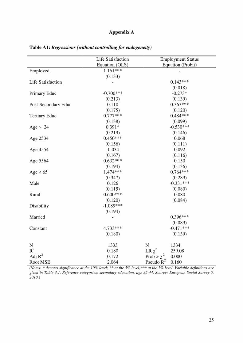
Appendix A
Table A1: Regressions (without controlling for endogeneity)
Life Satisfaction
Equation (OLS)
Employment Status
Equation (Probit)
Employed 1.161***
(0.133)
-
Life Satisfaction -
0.143***
(0.018)
Primary Educ -0.700***
(0.213)
-0.273*
(0.139)
Post-Secondary Educ 0.110
(0.175)
0.363***
(0.120)
Tertiary Educ 0.777***
(0.138)
0.484***
(0.099)
Age ≤ 24 0.391*
(0.219)
-0.530***
(0.146)
Age 2534 0.450***
(0.156)
0.068
(0.111)
Age 4554 -0.034
(0.167)
0.092
(0.116)
Age 5564 0.632***
(0.194)
0.150
(0.136)
Age ≥ 65 1.474***
(0.347)
0.764***
(0.289)
Male 0.126
(0.115)
-0.331***
(0.080)
Rural
0.600***
(0.120)
0.080
(0.084)
Disability -1.089***
(0.194)
Married - 0.396***
(0.089)
Constant 4.733***
(0.180)
-0.471***
(0.139)
N 1333 N 1334
R2 0.180 LR χ
2 259.08
Adj R2 0.172 Prob > χ
2 0.000
Root MSE 2.064 Pseudo R2 0.160
(Notes: * denotes significance at the 10% level; ** at the 5% level;*** at the 1% level. Variable definitions are
given in Table 3.1. Reference categories: secondary education, age 35-44. Source: European Social Survey 5,
2010.)

26
Appendix B
Table B1: Two-Stage Probit Least Squares Results (controlling for endogeneity) –
Alternative Dependent Variable ‘Happy’
Happiness
Equation
Employment Status
Equation
Employed 1.570***
(0.367)
-
Happy -
0.349***
(0.110)
Primary Educ -0.491
(0.305)
-0.001*
(0.187)
Post-Secondary Educ -0.129
(0.267)
0.213
(0.136)
Tertiary Educ 0.080
(0.300)
0.241
(0.154)
Age ≤ 24 1.036**
(0.368)
-0.572***
(0.157)
Age 2534 0.308
(0.208)
-0.039
(0.133)
Age 4554 -0.210
(0.225)
0.118
(0.120)
Age 5564 0.215
(0.282)
0.046
(0.155)
Age ≥ 65 -0.141
(0.637)
0.515
(0.327)
Male 0.498**
(0.188)
-0.318***
(0.083)
Rural
0.189
(0.174)
-0.005*
(0.099)
Disability -0.548*
(0.307)
Married - 0.208*
(0.127)
Constant 5.231***
(0.272)
-1.692**
(0.612)
N 1334 N 1334
R2 0.183 LR χ
2 206.23
Adj R2 0.176 Prob > χ
2 0.000
Root MSE 1.933 Pseudo R2 0.128
(Notes: * denotes significance at the 10% level; ** at the 5% level;*** at the 1% level. Dependent variable
‘happy’. Reference categories: secondary education, age 35-44. Source: European Social Survey 5, 2010.)
27
Table B2: Two-Stage Probit Least Squares Results (controlling for endogeneity) -
Alternative Dependent Variable ‘Wellbeing’
Wellbeing
Equation
Employment Status
Equation
Employed 0.842**
(0.381)
-
Wellbeing -
0.240***
(0.073)
Primary Educ -0.764**
(0.327)
-0.125
(0.164)
Post-Secondary Educ -0.431
(0.279)
0.397***
(0.124)
Tertiary Educ -0.172
(0.310)
0.511***
(0.105)
Age ≤ 24 1.145**
(0.396)
-0.657***
(0.165)
Age 2534 0.767***
(0.216)
-0.068
(0.136)
Age 4554 -0.058
(0.234)
0.090
(0.120)
Age 5564 0.279
(0.291)
0.145
(0.144)
Age ≥ 65 0.188
(0.631)
0.778**
(0.299)
Male 0.618**
(0.196)
-0.400***
(0.087)
Rural
0.122
(0.180)
0.092
(0.089)
Disability -1.453***
(0.328)
Married - 0.364***
(0.098)
Constant 12.557***
(0.290)
-2.762**
(0.916)
N 1333 N 1333
R2 0.083 LR χ
2 206.19
Adj R2 0.075 Prob > χ
2 0.000
Root MSE 2.734 Pseudo R2 0.128
(Notes: * denotes significance at the 10% level; ** at the 5% level;*** at the 1% level. Dependent variable
‘wellbeing’. Reference categories: secondary education, age 35-44. Source: European Social Survey 5, 2010.)