scientia magna, 5, no. 3
DESCRIPTION
Papers in science (mathematics, physics, philosophy, psychology, sociology, linguistics).TRANSCRIPT


Vol. 5, No. 3, 2009 ISSN 1556-6706
SCIENTIA MAGNA
An international journal
Edited by
Department of Mathematics Northwest University
Xi’an, Shaanxi, P.R.China

i
Scientia Magna is published annually in 400-500 pages per volume and 1,000 copies. It is also available in microfilm format and can be ordered (online too) from:
Books on Demand ProQuest Information & Learning 300 North Zeeb Road P.O. Box 1346 Ann Arbor, Michigan 48106-1346, USA Tel.: 1-800-521-0600 (Customer Service) URL: http://wwwlib.umi.com/bod/ Scientia Magna is a referred journal: reviewed, indexed, cited by the following journals: "Zentralblatt Für Mathematik" (Germany), "Referativnyi Zhurnal" and "Matematika" (Academia Nauk, Russia), "Mathematical Reviews" (USA), "Computing Review" (USA), Institute for Scientific Information (PA, USA), "Library of Congress Subject Headings" (USA).
Printed in the United States of America Price: US$ 69.95
ii
Information for Authors
Papers in electronic form are accepted. They can be e-mailed in Microsoft Word XP (or lower), WordPerfect 7.0 (or lower), LaTeX and PDF 6.0 or lower.
The submitted manuscripts may be in the format of remarks, conjectures, solved/unsolved or open new proposed problems, notes, articles, miscellaneous, etc. They must be original work and camera ready [typewritten/computerized, format: 8.5 x 11 inches (21,6 x 28 cm)]. They are not returned, hence we advise the authors to keep a copy.
The title of the paper should be writing with capital letters. The author's name has to apply in the middle of the line, near the title. References should be mentioned in the text by a number in square brackets and should be listed alphabetically. Current address followed by e-mail address should apply at the end of the paper, after the references.
The paper should have at the beginning an abstract, followed by the keywords. All manuscripts are subject to anonymous review by three independent
reviewers. Every letter will be answered. Each author will receive a free copy of the journal.

iii
Contributing to Scientia Magna Authors of papers in science (mathematics, physics, philosophy, psychology,
sociology, linguistics) should submit manuscripts, by email, to the Editor-in-Chief:
Prof. Wenpeng Zhang Department of Mathematics Northwest University Xi’an, Shaanxi, P.R.China E-mail: [email protected]
Or anyone of the members of Editorial Board: Dr. W. B. Vasantha Kandasamy, Department of Mathematics, Indian Institute of Technology, IIT Madras, Chennai - 600 036, Tamil Nadu, India. Dr. Larissa Borissova and Dmitri Rabounski, Sirenevi boulevard 69-1-65, Moscow 105484, Russia. Dr. Zhaoxia Wu, School of Applied Mathematics, Xinjiang University of Finance and Economics, Urmq, P.R.China. E-mail: [email protected] Prof. Yuan Yi, Research Center for Basic Science, Xi’an Jiaotong University, Xi’an, Shaanxi, P.R.China. E-mail: [email protected] Dr. Zhefeng Xu, Department of Mathematic s, Northwest University, Xi’an, Shaanxi, P.R.China. E-mail: [email protected]; [email protected] Prof. József Sándor, Babes-Bolyai University of Cluj, Romania. E-mail: [email protected]; [email protected] Dr. Xia Yuan, Department of Mathematics, Northwest University, Xi’an, Shaanxi, P.R.China. E-mail: [email protected]

Contents
Y. Wang : On the mean value of SSMP (n) and SIMP (n) 1
K. Ratanavongsawad : A family of Beta-Fibonacci sequences 6
J. Sandor : The product of divisors minimum and maximum functions 13
S. Shakeri, etc. : Generalized random stability of Jensen type mapping 19
C. Prabpayak and U. Leerawat : On Isomorphisms of KU-algebras 25
S. M. Khairnar, etc. : Smarandache friendly numbers-another approach 32
E. Ozyılmaz, etc. : Simple closed null curves in Minkowski 3-Space 40
M. K. Karacan and B. Bukcu : On the Elliptic cylindrical Tzitzeica curves in Minkowski
3-Space 44
N. Dung and V. Hang : On n-Frechet spaces 49
K. Thirugnanasambandam and S. Panayappan : Product of powers of quasinormal
composition operators 56
S. M. Khairnar, etc. : Smarandache magic square 60
S. Balasubramanian : Pairwise semi compact and pairwise semi lindeloff spaces 62
J. Sandor : A note on f -minimum functions 72
G. Zheng : Some Smarandache conclusions of coloring properties of complete uniform
mixed hypergraphs deleted some C-hyperedges 76
Q. Zhao and Y. Wang : A limit problem of the Smarandache dual function S∗∗(n) 87
B. Amudhambigai, etc. : Separation axioms in smooth fuzzy topological spaces 91
X. Yan : An integral identity involving the Hermite polynomials 100
H. Zhao, etc. : Vinegar identification by ultraviolet spectrum technology and pattern
recognition method 104
A. H. Majeed and A. D. Hamdi : (σ, τ)-derivations on Jordan ideals 112
H. Jolany and M. R. Darafsheh : Some another remarks on the generalization of
Bernoulli and Euler numbers 118
iv

Scientia MagnaVol. 5 (2009), No. 3, 1-5
On the mean value of SSMP (n) and SIMP (n)1
Yiren Wang
Department of Mathematics, Northwest University, Xi’an, Shaanxi, P.R.China
Abstract The main purpose of this paper it to studied the mean value properties of the
Smarandache Superior m-th power part sequence SSMP (n) and the Smarandache Inferior
m-th power part sequence SIMP (n), and give several interesting asymptotic formula for
them.
Keywords Smarandache Superior m-th power part sequence, Smarandache Inferior m-th
power part sequences, mean value, asymptotic formula.
§1. Introduction and Results
For any positive integer n, the Smarandache Superior m-th power part sequence SSMP (n)is defined as the smallest m-th power greater than or equal to n. The Smarandache Inferiorm-th power part sequence SIMP (n) is defined as the largest m-th power less than or equal ton. For example, if m = 2, then the first few terms of SIMP (n) are: 0, 1, 1, 1, 4, 4, 4, 4, 4, 9,9, 9, 9, 9, 9, 9, 16, 16, 16, 16, 16, 16, 16, 16, 16, 25, · · · . The first few terms of SSMP (n) are:1, 4, 4, 4, 9, 9, 9, 9, 9, 16, 16, 16, 16, 16, 16, 16, 25, · · · . If m = 3, then The first few terms ofSSMP (n) are: 1, 8, 8, 8, 8, 8, 8, 8, 27, 27, 27, 27, 27, 27, 27, 27, 27, 27, 27, 27, 27, 27, 27, 27,27, 27, 27, 64, · · · . The first few terms of SIMP (n) are: 0, 1, 1, 1, 1, 1, 1, 1, 8, 8, 8, 8, 8, 8, 8,8, 8, 8, 8, 8, 8, 8, 8, 8, 8, 8, 8, 27, · · · . Now we let
Sn = (SSMP (1) + SSMP (2) + · · ·+ SSMP (n))/n;
In = (SIMP (1) + SIMP (2) + · · ·+ SIMP (n))/n;
Kn = n√
SSMP (1) + SSMP (2) + · · ·+ SSMP (n);
In = n√
SIMP (1) + SIMP (2) + · · ·+ SIMP (n).
In reference [2], Dr. K.Kashihara asked us to study the properties of these sequences. Gou Su[3] studied these problem, and proved the following conclusion:
For any real number x > 2 and integer m = 2, we have the asymptotic formula
∑
n6x
SSSP (n) =x2
2+ O
(x
32
),
∑
n6x
SISP (n) =x2
2+ O
(x
32
),
and
Sn
In= 1 + O
(n−
12
), lim
n→∞Sn
In= 1.
1This work is supported by the Shaanxi Provincial Education Department Foundation 08JK433.

2 Yiren Wang No. 3
In this paper, we shall use the elementary method to give a general conclusion. That is,we shall prove the following:
Theorem 1. Let m ≥ 2 be an integer, then for any real number x > 1, we have theasymptotic formula
∑
n≤x
SSMP (n) =x2
2+ O
(x
2m−1m
),
and ∑
n≤x
SIMP (n) =x2
2+ O
(x
2m−1m
).
Theorem 2. For any fixed positive integer m ≥ 2 and any positive integer n, we havethe asymptotic formula
Sn − In =m(m− 1)2m− 1
n1− 1m + O
(n1− 2
m
).
Corollary 1. For any positive integer n, we have the asymptotic formula
Sn
In= 1 + O
(n−
1m
),
and the limit limn→∞
Sn
In= 1.
Corollary 2. For any positive integer n, we have the asymptotic formula
Kn
Ln= 1 + O
(1n
),
and the limit limn→∞
Kn
Ln= 1, lim
n→∞(Kn − Ln) = 0.
§2. Proof of the theorems
In this section, we shall use the Euler summation formula and the elementary method tocomplete the proof of our Theorems. For any real number x > 2, it is clear that there existsone and only one positive integer M satisfying Mm < x ≤ (M +1)m. That is, M = x
1m +O(1).
So we have∑
n≤x
SSMP (n) =∑
n≤Mm
SSMP (n) +∑
Mm<n≤x
SSMP (n)
=∑
k≤M
(km − (k − 1)m)km + ([x]− (Mm + 1))(M + 1)m
=∑
k≤M
(mk2m−1 + O(k2m−2)) + ([x]−Mm − 1)(M + 1)m
=m ·M2m
2m+ O
(M2m−1
)+ ([x]−Mm − 1) (M + 1)m
=M2m
2+ O
(M2m−1
).

Vol. 5 On the mean value of SSMP (n) and SIMP (n) 3
Note that M = x1m + O(1), from the above estimate we have the asymptotic formula
∑
n≤x
SSMP (n) =x2
2+ O
(x2− 1
m
).
This proves the first formula of Theorem 1.Now we prove the second one. For any real number x > 1, we also have
∑
n≤x
SIMP (n) =∑
n<Mm
SIMP (n) +∑
Mm≤n≤x
SIMP (n)
=∑
k6M
(km − (k − 1m))(k − 1)m +∑
Mm6n6x
Mm
=∑
k6M
(mk2m−1 + O(k2m−2)) + ([x]−Mm + 1) Mm
=M2m
2+ O
(M2m−1
)+ ([x]−Mm + 1) Mm.
Note that
([x]−Mm + 1) Mm 6 M2m−1 ≤ x1− 1m .
Therefore,∑
n≤x
SSMP (n) =x2
2+ O
(x2− 1
m
).
This completes the proof of Theorem 1.To prove Theorem 2, let x = n, then from the method of proving Theorem 1 we have
Sn − In =1n
(SSMP (1) + SSMP (2) + · · ·+ SSMP (n))
− 1n
(SIMP (1) + SIMP (2) + · · ·+ SIMP (n))
=1n
∑
k≤M
(km − (k − 1)m)km + ([x]− (Mm + 1))(M + 1)m
− 1n
∑
k6M
(km − (k − 1m))(k − 1)m + ([x]−Mm + 1)Mm
=1n
∑
k≤M
m(m− 1)k2m−2 + O
(1n
M2m−2
)
=m(m− 1)n(2m− 1)
M2m−1 + O
(1n
M2m−2
).
Note that Mm < n ≤ (M+1)m or M = n1m +O(1), from the above formula we may immediately
deduce that
Sn − In =m(m− 1)2m− 1
n1− 1m + O
(n1− 2
m
).
This completes the proof of Theorem 2.

4 Yiren Wang No. 3
Now we prove the Corollaries. Note that the asymptotic formula
In =1n
(SIMP (1) + SIMP (2) + · · ·+ SIMP (n)) =1n
(n2
2+ O
(n
2m−1m
))=
n
2+ O
(n1− 1
m
)
and
Sn =1n
(SSMP (1) + SSMP (2) + · · ·+ SSMP (n)) =1n
(n2
2+ O
(n
2m−1m
))=
n
2+O
(n1− 1
m
).
From the above two formula we have
Sn
In=
n2 + O
(n
m−1m
)
n2 + O
(n
m−1m
) = 1 + O(n−
1m
).
Therefore, we have the limit formula
limn→∞
Sn
In= 1.
Using the same method we can also deduce that
Kn = n√
SSMP (1) + SSMP (2) + · · ·+ SSMP (n) =(
n2
2+ O
(n
2m−1m
)) 1n
and
Ln = n√
SIMP (1) + SIMP (2) + · · ·+ SIMP (n) =(
n2
2+ O
(n
2m−1m
)) 1n
From these formula we may immediately deduce that
Kn
Ln=
n2
2 + O(n
2m−1m
)
n2
2 + O(n
2m−1m
)
1n
=(1 + O
(n−
1m
)) 1n
= 1 + O
(1n
).
Therefore, we have the limit formula
limn→∞
Kn
Ln= 1.
Note that limn→∞
Kn = limn→∞
Ln = 1, we may immediately deduce that
limn→∞
(Kn − Ln) = 0.
This completes the proof of Corollary 2.
References
[1] F. Smarandache, Only Problems, Not Solutions, Chicago: Xiquan Publishing House,1993.
[2] Kenichiro Kashihara, Comments and topics on Smarandache notions and problems,Erhus University Press, USA, 1996.

Vol. 5 On the mean value of SSMP (n) and SIMP (n) 5
[3] Gou Su, On the mean values of SSSP(n) and SISP(n), Pure and Applied Mathematics,Vol. 25(2009), No. 3, 431-434.
[4] M. L. Perez, Florentin Smarandache Definitions, Solved and Unsolved Problems, Con-jectures and Theorems in Number theory and Geometry, Chicago: Xiquan Publishing House,2000.
[5] F. Smarandache, Sequences of Numbers Involved in Unsolved Problems, Hexis, 2006.[6] Shen Hong, A new arithmetical function and its the value distribution, Pure and Applied
Mathematics, Vol. 23(2007), No. 2, 235-238.[7] Tom M. Apostol, Introduction to Analytical Number Theory, New York: Spring-Verlag,
1976.[8] Du Fengying, On a conjecture of the Smarandache function S(n), Vol. 23(2007), No.
2, 205-208.[9] Xu Zhefeng, The value distribution property of the Smarandache function, Acta Math-
ematica Sinica, Chinese Series, Vol. 49(2006), No. 5, 1009-1012.[10] Charles Ashbacher, Some problems on Smarandache function, Smarandache Notions
Journal, Vol. 6(1995), No. 1-2-3, 21-36.[11] Zhang Wenpeng, The elementary number theory (in Chinese), Shaanxi Normal Uni-
versity Press, Xi’an, 2007.[12] Liu Hongyan and Zhang Wenpeng, A number theoretic function and its mean value
property, Smarandache Notions Journal, Vol. 13(2002), No. 1-2-3, 155-159.[13] Wu Qibin, A composite function involving the Smarandache function, Pure and Ap-
plied Mathematics, Vol. 23(2007), No. 4, 463-466.[14] Yi Yuan and Kang Xiaoyu, Research on Smarandache Problems (in Chinese), High
American Press, 2006.[15] Chen Guohui, New Progress On Smarandache Problems (in Chinese), High American
Press, 2007.[16] Liu Yanni, Li Ling and Liu Baoli, Smarandache Unsolved Problems and New Progress
(in Chinese), High American Press, 2008.[17] Wang Yu, Su Juanli and Zhang Jin, On the Smarandache Notions and Related Prob-
lems (in Chinese), High American Press, 2008.[18] Li Jianghua and Guo Yanchun, Research on Smarandache Unsolved Problems (in
Chinese), High American Press, 2009.[19] Maohua Le, Some problems concerning the Smarandache square complementary func-
tion (IV), Smarandache Notions Journal, Vol. 14(2004), No. 2, 335-337.[20] Liu Yaming, On the solutions of an equation involving the Smarandache function,
Scientia Magna, Vol. 2(2006), No. 1, 76-79.

Scientia MagnaVol. 5 (2009), No. 3, 6-12
A family of Beta-Fibonacci sequences
Krongtong Ratanavongsawad
Department of Mathematics Kasetsart University, Bangkok, ThailandE-mail: [email protected]
Abstract This paper gives a generalization of Beta-nacci and Fibonacci sequences and the
general solution obtained is given in terms of Beta-Fibonacci numbers.
Keywords Beta-nacci sequence, Fibonacci sequence.
§1. Preliminaries and introduction
The Fibonacci sequence, say Fn∞n=0 is defined recurrently by
Fn = Fn−1 + Fn−2, for all n ≥ 2, (1)
with initial conditions
F0 = 1; F1 = 1.
The general term of the Fibonacci sequence is
Fn =1√5
(1 +
√5
2
)n+1
− 1√5
(1−√5
2
)n+1
.
The Fibonacci sequence has been studied extensively and generalized in many ways. In [1]Peter R. J. Asveld studied the class of recurrence relations
Gn = Gn−1 + Gn−2 +k∑
j=0
αjnj (2)
with initial conditions
G0 = 1; G1 = 1.
The main result of [1] consists of an expression for Gn in terms of the Fibonacci numbersFn and Fn−1, and in the parameters α0, α1, ..., αk.
The Beta-nacci sequence, say Bn∞n=0 is defined recurrently by
Bn = Bn−1 + 2Bn−2, for all n ≥ 2, (3)

Vol. 5 A family of Beta-Fibonacci sequences 7
with initial conditions
B0 = 1; B1 = 1.
The general term of the Beta-nacci sequence is
Bn =2n+1 + (−1)n
3.
In this paper, we give a generalized of Beta-nacci sequences and the general solution ob-tained is given in terms of Beta-nacci numbers. Also we consider a generalization of the Fi-bonacci and the Beta-nacci sequences, then we define a new recurrence, which we call theBeta-Fibonacci sequence. Further, we give a generalization of Beta-Fibonacci sequence, calledthe generalized BF-nacci sequence and express the nth term of the generalized BF-nacci se-quence in terms of the Beta-Fibonacci numbers.
§2. A generalization of Beta-nacci sequence
Definition. For any non-negative integer k and any real numbers α0, α1, · · · , αk, a gen-eralization of Beta-nacci sequence Sn∞n=0 is defined recurrently by
Sn = Sn−1 + 2Sn−2 +k∑
j=0
αjnj , for all n ≥ 2, (4)
with initial conditions
S0 = 1; S1 = 1.
Theorem 1. The solution of (4) can be express as
Sn = (1− Λk)Bn + ΨkBn−1 +k∑
j=0
pj(n)αj , (5)
where(i) Λk is a linear combination of α0, α1, · · · , αk;(ii) Ψk is a linear combination of α1, · · · , αk ;(iii) for each j ( 0 ≤ j ≤ k ), pj(n) is a polynomail of degree j.Proof of Theorem 1. First, we solve the homogeneous recurrence relation
Sn = Sn−1 + 2Sn−2.
The characteristic polynomail, x2 − x− 2, has distinct roots 2 and −1, so the solution is
S(h)n = c12n + c2(−1)n,
where c1 and c2 are constants.

8 Krongtong Ratanavongsawad No. 3
Next we find the particular solution of (4).
We set S(p)n =
k∑
i=0
Aini, and attempt to determine A0, A1, ..., Ak.
Putting this expression for S(p)n in (4), we obtain
k∑
i=0
Aini =
k∑
i=0
Ai(n− 1)i + 2k∑
i=0
Ai(n− 2)i +k∑
i=0
αini.
Hence, for each i = 0, 1, · · · , k, we get
Ai −k∑
m=i
βimAm − αi = 0 (6)
with, for m ≥ i,
βim =(
m
i
)(−1)m−i(1 + 2m−i+1).
From the recurrence relation (6), we can successively determine Ak, Ak−1, · · · , A0 : the coeffi-cient Ai is a linear combination of αi, αi+1, · · · , αk.Therefore, we set
Ai =k∑
j=i
cijαj , (7)
which yields, together with (6),
k∑
j=i
cijαj −k∑
m=i
βim
( k∑
j=m
cmjαj
)− αi = 0.
Thus, for 0 ≤ i ≤ j ≤ k, we have
cjj = −12
cij = −12
( j∑
m=i+1
βimcmj
)for i < j.
Therefore the particular solution S(p)n of (4), we obtain
S(p)n =
k∑
i=0
( k∑
j=i
cijαj
)ni
=k∑
j=0
( j∑
i=0
cijni
)αj .

Vol. 5 A family of Beta-Fibonacci sequences 9
Finally, the recurrence relation (4) has the solution
Sn = S(h)n + S(p)
n
= c12n + c2(−1)n +k∑
j=0
( j∑
i=0
cijni
)αj .
The initial conditions: S0 = 1; S1 = 1, give
c1 =23− 1
3
(2Λk −Ψk
)
c2 =13− 1
3
(Λk + Ψk
),
where
Λk =∑k
j=0 c0jαj
and
Ψk =
0, if k = 0;
−∑kj=1
(∑ji=1 cij
)αj , if k > 0.
Since Bn =2n+1 + (−1)n
3, Sn can be written as
Sn = (1− Λk)Bn + ΨkBn−1 +k∑
j=0
pj(n)αj ,
where
pj(n) =j∑
i=0
cijni.
The proof of the Theorem is now complete.
§3. A generalization of the Fibonacci and Beta-nacci se-
quences
In this section, we consider a generalization of the Fibonacci and Beta-nacci sequences.First, we define the Beta - Fibonacci sequence as follows:
Definition. Let r be a non-negative integer such that r ≥ 0. Define the Beta-Fibonaccisequence Tn∞n=0 as shown:
Tn = Tn−1 + 2rTn−2 for all n ≥ 2, (8)

10 Krongtong Ratanavongsawad No. 3
with initial conditions
T0 = 1; T1 = 1.
When r = 0, then the sequence Tn∞n=0 is reduced to the Fibonacci sequence Fn∞n=0
and when r = 1 , the sequence Tn∞n=0 is reduced to the Beta-nacci sequence Bn∞n=0.The general term of the Beta-Fibonacci sequence is
Tn =1√
1 + 2r+2
(φn+1
1 − φn+12
),
where
φ1 =12(1 +
√1 + 2r+2) and φ2 =
12(1−
√1 + 2r+2)
Now we define a generalization of the Beta-Fibonacci sequence, we call generalized BF-naccisequence.
Definition. Let r be a non-negative integer such that r ≥ 0. For any non-negative integerk and any real numbers α0, α1, · · · , αk, a generalized BF-nacci sequence Rn∞n=0 is definedrecurrently by
Rn = Rn−1 + 2rRn−2 +k∑
j=0
αjnj , for all n ≥ 2, (9)
with initial conditions
R0 = 1; R1 = 1.
Note that if we take r = 0 in the definition, the sequence Rn∞n=0 is reduced to the gener-alization of the Fibonacci sequence Gn∞n=0 as shown in [1]. Also when r = 1, the sequenceRn∞n=0 is reduced to the generalization of the Beta - nacci sequence Sn∞n=0 .
Theorem 2. The solution of (9) can be express as
Rn = (1− Λk)Rn + ΨkRn−1 +k∑
j=0
pj(n)αj , (10)
where(i) Λk is a linear combination of α0, α1, · · · , αk;(ii) Ψk is a linear combination of α1, · · · , αk;(iii) for each j ( 0 ≤ j ≤ k ), pj(n) is a polynomail of degree j.Proof of Theorem 2. As usual the solution R
(h)n of the homogeneous equation corre-
sponding to (9) is
R(h)n = c1φ
n1 + c2φ
n2 ,
where
φ1 =12(1 +
√1 + 2r+2) and φ2 =
12(1−
√1 + 2r+2).

Vol. 5 A family of Beta-Fibonacci sequences 11
Next, we find the particular solution of (9) . We set R(p)n =
k∑
i=0
Aini, which yields
k∑
i=0
Aini =
k∑
i=0
Ai(n− 1)i + 2rk∑
i=0
Ai(n− 2)i +k∑
i=0
αini.
Thus, for each i = 0, 1, · · · , k, we have
Ai −k∑
m=i
βimAm − αi = 0 (11)
with, for m ≥ i,
βim =(
m
i
)(−1)m−i(1 + 2m−i+r).
From the recurrence relation (11), we can successively determine Ak, Ak−1, · · · , A0 :the coefficient Ai is a linear combination of αi, αi+1, · · · , αk.
Therefore, we set
Ai =k∑
j=i
cijαj , (12)
which yields, together with (11),
k∑
j=i
cijαj −k∑
m=i
βim
( k∑
j=m
cmjαj
)− αi = 0.
Thus, for 0 ≤ i ≤ j ≤ k, we have
cjj = − 12r
cij = − 12r
( j∑
m=i+1
βimcmj
)for i < j.
Hence, for the particular solution R(p)n of (9), we obtain
R(p)n =
k∑
i=0
( k∑
j=i
cijαj
)ni
=k∑
j=0
( j∑
i=0
cijni
)αj .

12 Krongtong Ratanavongsawad No. 3
Finally, the recurrence relation (9) has the solution
Rn = R(h)n + R(p)
n
= c1φn1 + c2φ
n2 +
k∑
j=0
( j∑
i=0
cijni
)αj .
The initial conditions: R0 = 1; R1 = 1, give
c1 =1√
1 + 2r+2
((1−R
(p)0 )φ1 + R
(p)0 −R
(p)1
)
c2 = − 1√1 + 2r+2
((1−R
(p)0 )φ2 + R
(p)0 −R
(p)1
)
Since Tn =1√
1 + 2r+2
(φn+1
1 − φn+12
), Rn can be written as
Rn = (1−R(p)0 )Tn + (R(p)
0 −R(p)1 )Tn−1 +
k∑
j=0
pj(n)αj ,
where
pj(n) =j∑
i=0
cijni.
Hence the proof is complete.
Acknowledgement
The author would like to thank to the anonymous referee for helpful suggestions.
References
[1] Asveld, Peter R. J., A family of Fibonacci like sequences, The Fibonacci Quarterly,25(1987), 81-83.
[2] Balakrishnan, V.K., Combinatorics, Singapore, McGraw-Hill Book Co. (1995).[3] Levine, Shari Lynn, Suppose mose rabbits are born, The Fibonacci Quarterly, 26(1988),
306 -311.

Scientia MagnaVol. 5 (2009), No. 3, 13-18
The product of divisors minimum andmaximum functions
Jozsef Sandor
Babes-Bolyai University of Cluj, RomaniaE-mail: [email protected] [email protected]
Abstract Let T (n) denote the product of divisors of the positive integer n. We introduce
and study some basic properties involving two functions, which are the minimum, resp. the
maximum of certain integers connected with the divisors of T(n).
Keywords Arithmetic functions, product of divisors of an integer.
1. Let T (n) =∏i|n
i denote the product of all divisors of n. The product-of-divisors
minimum, resp. maximum functions will be defined by
T (n) = mink ≥ 1 : n|T (k) (1)
andT∗(n) = maxk ≥ 1 : T (k)|n. (2)
There are particular cases of the functions FAf , GA
g defined by
FAf (n) = mink ∈ A : n|f(k), (3)
and its ”dual”GA
g (n) = maxk ∈ A : g(k)|n, (4)
where A ⊂ N∗ is a given set, and f, g : N∗ → N are given functions, introduced in [8] and [9].For A = N∗, f(k) = g(k) = k! one obtains the Smarandache function S(n), and its dual S∗(n),given by
S(n) = mink ≥ 1 : n|k! (5)
andS∗(n) = maxk ≥ 1 : k!|n. (6)
The function S∗(n) has been studied in [8], [9], [4], [1], [3]. For A = N∗, f(k) = g(k) = ϕ(k),one obtains the Euler minimum, resp. maximum functions
E(n) = mink ≥ 1 : n|ϕ(k) (7)
studied in [6], [8], [13], resp., its dual
E∗(n) = maxk ≥ 1 : ϕ(k)|n, (8)

14 Jozsef Sandor No. 3
studied in [13].For A = N∗, f(k) = g(k) = S(k) one has the Smarandache minimum and maximum
functionsSmin(n) = mink ≥ 1 : n|S(k), (9)
Smax(n) = maxk ≥ 1 : S(k)|n, (10)
introduced, and studied in [15]. The divisor minimum function
D(n) = mink ≥ 1 : n|d(k) (11)
(where d(k) is the number of divisors of k) appears in [14], while the sum-of-divisors minimumand maximum functions
Σ(n) = mink ≥ 1 : n|σ(k) (12)
Σ∗(n) = maxk ≥ 1 : σ(k)|n (13)
have been recently studied in [16].For functions Q(n), Q1(n) obtained from (3) for f(k) = k! and A = set of perfect squares,
resp. A = set of squarefree numbers, see [10].2. The aim of this note is to study some properties of the functions T (n) and T∗(n) given
by (1) and (2). We note that properties of T (n) in connection with ”multiplicatively perfectnumbers” have been introduced in [11]. For other asymptotic properties of T (n), see [7]. Fordivisibility properties of T (σ(n)) with T (n), see [5]. For asymptotic results of sums of type∑n≤x
1T (n) , see [17].
A divisor i of n is called ”unitary” if(i, n
i
)= 1. Let T ∗(n) be the product of unitary
divisors of n. For similar results to [11] for T ∗(n), or T ∗∗(n) (i.e. the product of ”bi-unitary”divisors of n), see [2]. The product of ”exponential” divisors Te(n) is introduced in paper [12].Clearly, one can introduce functions of type (1) and (2) for T (n) replaced with one of the abovefunctions T ∗(n), T ∗∗, Te(n), but these functions will be studied in another paper.
3. The following auxiliary result will be important in what follows.Lemma 1.
T (n) = nd(n)/2, (14)
where d(n) is the number of divisors of n.Proof. This is well-known, see e.g. [11].Lemma 2.
T (a)|T (b), if a|b. (15)
Proof. If a|b, then for any d|a one has d|b, so T (a)|T (b). Reciprocally, if T (a)|T (b),let γp(a) be the exponent of the prime in a. Clearly, if p|a, then p|b, otherwise T (a)|T (b) isimpossible. If pγp(b)‖b, then we must have γp(a) ≤ γp(b). Writing this fact for all prime divisorsof a, we get a|b.
Theorem 1. If n is squarefree, then
T (n) = n. (16)

Vol. 5 The product of divisors minimum and maximum functions 15
Proof. Let n = p1p2 . . . pr, where pi (i = 1, r) are distinct primes. The relation p1p2 . . . pr|T (k)gives pi|T (k), so there is a d|k, so that pi|d. But then pi|k for all i = 1, r, thus p1p2 . . . pr = n|k.Since p1p2 . . . pk|T (p1p2 . . . pk), the least k is exactly p1p2 . . . pr, proving (16).
Remark. Thus, if p is a prime, T (p) = p; if p < q are primes, then T (pq) = pq, etc.Theorem 2. If a|b, a 6= b and b is squarefree, then
T (ab) = b. (17)
Proof. If a|b, a 6= b, then clearly T (b) =∏d|b
d is divisible by ab, so T (ab) ≤ b. Reciprocally,
if ab|T (k), let p|b a prime divisor of b. Then p|T (k), so (see the proof of Theorem 1) p|k. But b
being squarefree (i.e. a product of distinct primes), this implies b|k. The least such k is clearlyk = b.
For example, T (12) = T (2 · 6) = 6, T (18) = T (3 · 6) = 6, T (20) = T (2 · 10) = 10.Theorem 3. T (T (n)) = n for all n ≥ 1. (18)Proof. Let T (n)|T (k). Then by (15) one can write n|k. The least k with this property is
k = n, proving relation (18).Theorem 4. Let pi (i = 1, r) be distinct primes, and αi ≥ 1 positive integers. Then
max
T
(r∏
i=1
pαii
): i = 1, r
≤ T
(r∏
i=1
pαii
)≤
≤ l.c.m.[T (pα11 ), . . . , T (pαr
r )]. (19)
Proof. In [13] it is proved that for A = N∗, and any function f such that FN∗
f (n) = Ff (n)is well defined, one has
maxFf (pαii ) : i = 1, r ≤ Ff
(r∏
i=1
pαii
). (20)
On the other hand, if f satisfies the property
a|b =⇒ f(a)|f(b)(a, b ≥ 1), (21)
then
Ff
(r∏
i=1
pαii
)≤ l.c.m.[Ff (pα1
1 ), . . . , Ff (pαrr )]. (22)
By Lemma 2, (21) is true for f(a) = T (a), and by using (20), (22), relation (19) follows.Theorem 5.
T (2n) = 2α, (23)
where α is the least positive integer such that
α(α + 1)2
≥ n. (24)
Proof. By (14), 2n|T (k) iff 2n|kd(k)/2. Let k = pα11 . . . pαr
r , when d(k) = (α1+1) . . . (αr+1).Since 22n|kd(k) = p
α1(α1+1)...(αr+1)1 . . . p
αr(α1+1)...(αr+1)r (let p1 < p2 < · · · < pr), clearly p1 = 2

16 Jozsef Sandor No. 3
and the least k is when α2 = · · · = αr = 0 and α1 is the least positive integer with 2n ≤α1(α1 + 1). This proves (23), with (24).
For example, T (22) = 4, since α = 2, T (23) = 4 again, T (24) = 8 since α = 3, etc.For odd prime powers, the things are more complicated. For example, for 3n one has:Theorem 6.
T (3n) = min3α1 , 2 · 3α2, (25)
where α1 is the least positive integer such that α1(α1+1)2 ≥ n, and α2 is the least positive integer
such that α2(α2 + 1) ≥ n.Proof. As in the proof of Theorem 5,
32n|pα1(α1+1)...(αr+1)1 · pα2(α1+1)...(α1+1)
2 . . . pαr(α1+1)...(αr+1)r ,
where p1 < p2 < · · · < pr, so we can distinguish two cases:a) p1 = 2, p2 = 3, p3 ≥ 5;b) p1 = 3, p2 ≥ 5.Then k = 2α1 · 3α2 . . . pαr
r ≥ 2α1 · 3α2 in case a), and k ≥ 3α1 in case b). So for the leastk we must have α2(α1 + 1)(α2 + 1) ≥ 2n with α1 = 1 in case a), and α1(α1 + 1) ≥ 2n in caseb). Therefore α1(α1+1)
2 ≥ n and α2(α2 + 1) ≥ n, and we must select k with the least of 3α1 and21 · 3α2 , so Theorem 6 follows.
For example, T (32) = 6 since for n = 2, α1 = 2, α2 = 1, and min2 ·31, 32 = 6; T (33) = 9since for n = 3, α1 = 2, α2 = 2 and min2 · 32, 32 = 9.
Theorem 7. Let f : [1,∞) → [0,∞) be given by f(x) =√
x log x. Then
f−1(log n) < T (n) ≤ n, (26)
for all n ≥ 1, where f−1 denotes the inverse function of f .Proof. Since n|T (n), the right side of (26) follows by definition (1) of T (n). On the other
hand, by the known inequality d(k) < 2√
k, and Lemma 1 (see (14)) we get T (k) < k√
k, solog T (k) <
√k log k = f(k). Since n|T (k) implies n ≤ T (k), so log n ≤ log T (k) < f(k), and
the function f being strictly increasing and continuous, by the bijectivity of f , the left side of(26) follows.
4. The function T∗(n) given by (2) differs in many aspects from T (n). The first suchproperty is:
Theorem 8. T∗(n) ≤ n for all n, with equality only if n = 1 or n = prime.Proof. If T (k)|n, then T (k) ≤ n. But T (k) ≥ k, so k ≤ n, and the inequality follows.Let us now suppose that for n > 1, T∗(n) = n. Then T (n)|n, by definition 2. On the other
hand, clearly n|T (n), so T (n) = n. This is possible only when n = prime.Remark. Therefore the equality
T∗(n) = n(n > 1)
is a characterization of the prime numbers.Lemma 3. Let p1, . . . , pr be given distinct primes (r ≥ 1). Then the equation
T (k) = p1p2 . . . pr

Vol. 5 The product of divisors minimum and maximum functions 17
is solvable if r = 1.Proof. Since pi|T (k), we get pi|k for all i = 1, r. Thus p1 . . . pr|k, and Lemma 2 implies
T (p1 . . . pr)|T (k) = p1 . . . pr. Since p1 . . . pr|T (p1 . . . pr), we have T (p1 . . . pr) = p1 . . . pr, whichby Theorem 8 is possible only if r = 1.
Theorem 9. Let P (n) denote the greatest prime factor of n > 1. If n is squarefree, then
T∗(n) = P (n). (27)
Proof. Let n = p1p2 . . . pr, where p1 < p2 < · · · < pr. If T (k)|(p1 . . . pr), then clearlyT (k) ∈ 1, p1, . . . , pr, p1p2, . . . , p1p2 . . . pr. By Lemma 3 we cannot have
T (k) ∈ p1p2, . . . , p1p2 . . . pr,
so T (k) ∈ 1, p1, . . . , pr, when k ∈ 1, p1, . . . , pr. The greatest k is pr = P (n).Remark. Therefore T∗(pq) = q for p < q. For example, T∗(2 · 7) = 7, T∗(3 · 5) = 5,
T∗(3 · 7) = 7, T∗(2 · 11) = 11, etc.Theorem 10.
T∗(pn) = pα(p = prime), (28)
where α is the greatest integer with the property
α(α + 1)2
≤ n. (29)
Proof. If T (k)|pn, then T (k) = pm for m ≤ n. Let q be a prime divisor of k. Thenq = T (q)|T (k) = 2m implies q = p, so k = pα. But then T (k) = pα(α+1)/2 with α the greatestnumber such that α(α + 1)/2 ≤ n, which finishes the proof of (28).
For example, T∗(4) = 2, since α(α+1)2 ≤ 2 gives αmax = 1.
T∗(16) = 4, since α(α+1)2 ≤ 4 is satisfied with αmax = 2.
T∗(9) = 3, and T∗(27) = 9 since α(α+1)2 ≤ 3 with αmax = 2.
Theorem 11. Let p, q be distinct primes. Then
T∗(p2q) = maxp, q. (30)
Proof. If T (k)|p2q, then T (k) ∈ 1, p, q, p2, pq, p2q. The equations T (k) = p2, T (k) = pq,T (k) = p2q are impossible. For example, for the first equation, this can be proved as follows.By p|T (k) one has p|k, so k = pm. Then p(pm) are in T (k), so m = 1. But then T (k) = p 6= p2.For the last equation, k = (pq)m and pqm(pm)(qm)(pqm) are in T (k), which is impossible.
Theorem 12. Let p, q be distinct primes. Then
T∗(p3q) = maxp2, q. (31)
Proof. As above, T (k) ∈ 1, p, q, pq, p2q, p3q, p2, p3 and T (k) ∈ pq, p2q, p3q, p2 areimpossible. But T (k) = p3 by Lemma 1 gives kd(k) = p6, so k = pm, when d(k) = m + 1. Thisgives m(m + 1) = 6, so m = 2. Thus k = p2. Since p < p2 the result follows.
Remark. The equationT (k) = ps (32)

18 Jozsef Sandor No. 3
can be solved only if kd(k) = p2s, so k = pm and we get m(m + 1) = 2s. Therefore k = pm,with m(m + 1) = 2s, if this is solvable. If s is not a triangular number, this is impossible.
Theorem 13. Let p, q be distinct primes. Then
T∗(psq) =
maxp, q, if s is not a triangular number,
maxpn, q, if s = m(m+1)2 .
References
[1] K. Atanasov, Remark on Jozsef Sandor and Florian Luca’s theorem, C. R. Acad. Bulg.Sci. 55(2002), No. 10, 9-14.
[2] A. Bege, On multiplicatively unitary perfect numbers, Seminar on Fixed Point Theory,Cluj-Napoca, 2(2001), 59-63.
[3] M. Le, A conjecture concerning the Smarandache dual function, Smarandache NotionJ. 14(2004), 153-155.
[4] F. Luca, On a divisibility property involving factorials, C. R. Acad. Bulg. Sci. 53(2000),No. 6, 35-38.
[5] F. Luca, On the product of divisors of n and σ(n), J. Ineq. Pure Appl. Math. 4(2003),No. 2, 7 pp. (electronic).
[6] P. Moree and H. Roskam, On an arithmetical function related to Euler’s totient andthe discriminantor, Fib. Quart. 33(1995), 332-340.
[7] T. Salat and J. Tomanova, On the product of divisors of a positive integer, Math.Slovaca 52(2002), No. 3, 271-287.
[8] J. Sandor, On certain generalizations of the Smarandache function, Notes NumberTheory Discr. Math. 5(1999), No. 2, 41-51.
[9] J. Sandor, On certain generalizations of the Smarandache function, Smarandache No-tions J. 11(2000), No. 1-3, 202-212.
[10] J. Sandor, The Smarandache function of a set, Octogon Math. Mag. 9(2001), No. 1B,369-371.
[11] J. Sandor, On multiplicatively perfect numbers, J. Ineq. Pure Appl. Math. 2(2001),No. 1, 6 pp. (electronic).
[12] J. Sandor, On multiplicatively e-perfect numbers, (to appear).[13] J. Sandor, On the Euler minimum and maximum functions, (to appear).[14] J. Sandor, A note on the divisor minimum function, (to appear).[15] J. Sandor, The Smarandache minimum and maximum functions, (to appear).[16] J. Sandor, The sum-of-divisors minimum and maximum functions, (to appear).[17] Z. Weiyi, On the divisor product sequence, Smarandache Notions J., 14(2004), 144-
146.

Scientia MagnaVol. 5 (2009), No. 3, 19-24
Generalized random stability of Jensen typemapping
Saleh Shakeri ‡, Yeol Je Cho † and Reza Saadati ]
‡ Department of Mathematics, Islamic Azad University-Ayatollah Amoli branch, Amol P.O.Box 678, Iran
† Department of Mathematics Education and the RINS College of Education, GyeongsangNational University Chinju 660-701, Korea
] Faculty of Science, University of Shomal, Amol, P.O. Box 731, IranE-mail: [email protected] [email protected] [email protected]
Abstract In this paper, we consider Jensen type mapping in the setting of generalized random
normed spaces. We generalize a Hyers-Ulam stability result in the framework of classical
normed spaces.
Keywords Jensen type mapping, generalized random normed space.
§1. Introduction
In 1941 D.H. Hyers [5] solved this stability problem for additive mappings subject to theHyers condition on approximately additive mappings. In 1951 D.G. Bourgin [2] was the secondauthor to treat the Ulam stability problem for additive mappings. In 1978 P.M. Gruber [4]remarked that Ulam’s problem is of particular interest in probability theory and in the case offunctional equations of different types.
We wish to note that stability properties of different functional equations can have appli-cations to unrelated fields. For instance, Zhou [10] used a stability property of the functionalequation
f(x− y) + f(x + y) = 2f(x) (0.1)
to prove a conjecture of Z. Ditzian about the relationship between the smoothness of a mappingand the degree of its approximation by the associated Bernstein polynomials. In 2003–2006 J.M.Rassias and M.J. Rassias [6] and J.M. Rassias [7] solved the above Ulam problem for Jensenand Jensen type mappings. In this paper we consider the stability of Jensen type mapping inthe setting of intuitionistic fuzzy normed spaces.
§2. Preliminaries
In the sequel, we shall adopt the usual terminology, notations and conventions of the theoryof intuitionistic random normed spaces as in [8].

20 Saleh Shakeri, Yeol Je Cho and Reza Saadati No. 3
Definition 1. A measure distribution function is a function µ : R → [0, 1] which is leftcontinuous on R, non-decreasing and inft∈R µ(t) = 0, supt∈R µ(t) = 1.
We will denote by D the family of all measure distribution functions and by H a specialelement of D defined by
H(t) =
0 if t ≤ 0,
1 if t > 0.
If X is a nonempty set, then µ : X −→ D is called a probabilistic measure on X and µ(x)is denoted by µx.
Definition 2. A non-measure distribution function is a function ν : R → [0, 1] which isright continuous on R, non-increasing and inft∈R ν(t) = 1, supt∈R ν(t) = 0.
We will denote by B the family of all non-measure distribution functions and by G a specialelement of B defined by
G(t) =
1 if t ≤ 0,
0 if t > 0.
If X is a nonempty set, then ν : X −→ B is called a probabilistic non-measure on X andν(x) is denoted by νx.
lemma 1. [1,3] Consider the set L∗ and operation ≤L∗ defined by:
L∗ = (x1, x2) : (x1, x2) ∈ [0, 1]2 and x1 + x2 ≤ 1,
(x1, x2) ≤L∗ (y1, y2) ⇐⇒ x1 ≤ y1, x2 ≥ y2, ∀(x1, x2), (y1, y2) ∈ L∗.
Then (L∗,≤L∗) is a complete lattice.We denote its units by 0L∗ = (0, 1) and 1L∗ = (1, 0). Classically, a triangular norm ∗ = T
on [0, 1] is defined as an increasing, commutative, associative mapping T : [0, 1]2 −→ [0, 1]satisfying T (1, x) = 1 ∗ x = x for all x ∈ [0, 1]. A triangular conorm S = ¦ is defined as anincreasing, commutative, associative mapping S : [0, 1]2 −→ [0, 1] satisfying S(0, x) = 0 ¦ x = x
for all x ∈ [0, 1].
Using the lattice (L∗,≤L∗), these definitions can be straightforwardly extended.Definition 3. [3] A triangular norm (t–norm) on L∗ is a mapping T : (L∗)2 −→ L∗
satisfying the following conditions:(a) (∀x ∈ L∗)(T (x, 1L∗) = x) (boundary condition);(b) (∀(x, y) ∈ (L∗)2)(T (x, y) = T (y, x)) (commutativity);(c) (∀(x, y, z) ∈ (L∗)3)(T (x, T (y, z)) = T (T (x, y), z)) (associativity);(d) (∀(x, x′, y, y′) ∈ (L∗)4)(x ≤L∗ x′ and y ≤L∗ y′ =⇒ T (x, y) ≤L∗ T (x′, y′)) (monotonic-
ity).If (L∗,≤L∗ , T ) is an Abelian topological monoid with unit 1L∗ , then T is said to be a
continuous t–norm.Definition 4. [3] A continuous t–norm T on L∗ is said to be continuous t–representable
if there exist a continuous t–norm ∗ and a continuous t–conorm ¦ on [0, 1] such that, for allx = (x1, x2), y = (y1, y2) ∈ L∗,
T (x, y) = (x1 ∗ y1, x2 ¦ y2).

Vol. 5 Generalized random stability of Jensen type mapping 21
For example,T (a, b) = (a1b1,mina2 + b2, 1)
andM(a, b) = (mina1, b1,maxa2, b2)
for all a = (a1, a2), b = (b1, b2) ∈ L∗ are continuous t–representable.
Now, we define a sequence T n recursively by T 1 = T and
T n(x(1), · · · , x(n+1)) = T (T n−1(x(1), · · · , x(n)), x(n+1)), ∀n ≥ 2, x(i) ∈ L∗.
Definition 5. A negator on L∗ is any decreasing mapping N : L∗ −→ L∗ satisfyingN (0L∗) = 1L∗ and N (1L∗) = 0L∗ . If N (N (x)) = x for all x ∈ L∗, then N is called aninvolutive negator. A negator on [0, 1] is a decreasing mapping N : [0, 1] −→ [0, 1] satisfyingN(0) = 1 and N(1) = 0. Ns denotes the standard negator on [0, 1] defined by
Ns(x) = 1− x, ∀x ∈ [0, 1].
Definition 6. Let µ and ν be measure and non-measure distribution functions fromX × (0,+∞) to [0, 1] such that µx(t) + νx(t) ≤ 1 for all x ∈ X and t > 0. The triple(X,Pµ,ν , T ) is said to be an intuitionistic random normed space (briefly IRN-space) if X isa vector space, T is a continuous t–representable and Pµ,ν is a mapping X × (0,+∞) → L∗
satisfying the following conditions: for all x, y ∈ X and t, s > 0,(a) Pµ,ν(x, 0) = 0L∗ ;(b) Pµ,ν(x, t) = 1L∗ if and only if x = 0;(c) Pµ,ν(αx, t) = Pµ,ν(x, t
|α| ) for all α 6= 0;(d) Pµ,ν(x + y, t + s) ≥L∗ T (Pµ,ν(x, t),Pµ,ν(y, s)).
In this case, Pµ,ν is called an intuitionistic random norm. Here,
Pµ,ν(x, t) = (µx(t), νx(t)).
Example 1. Let (X, ‖ · ‖) be a normed space. Let T (a, b) = (a1b1,min(a2 + b2, 1)) forall a = (a1, a2), b = (b1, b2) ∈ L∗ and µ, ν be measure and non-measure distribution functionsdefined by
Pµ,ν(x, t) = (µx(t), νx(t)) =( t
t + ‖x‖ ,‖x‖
t + ‖x‖), ∀t ∈ R+.
Then (X,Pµ,ν , T ) is an IRN-space.Definition 7. (1) A sequence xn in an IRN-space (X,Pµ,ν , T ) is called a Cauchy
sequence if, for any ε > 0 and t > 0, there exists n0 ∈ N such that
Pµ,ν(xn − xm, t) >L∗ (Ns(ε), ε), ∀n,m ≥ n0,
where Ns is the standard negator.
(2) The sequence xn is said to be convergent to a point x ∈ X (denoted by xnPµ,ν−→ x)
if Pµ,ν(xn − x, t) −→ 1L∗ as n −→∞ for every t > 0.(3) An IRN-space (X,Pµ,ν , T ) is said to be complete if every Cauchy sequence in X is
convergent to a point x ∈ X.

22 Saleh Shakeri, Yeol Je Cho and Reza Saadati No. 3
§3. Stability results
Theorem 1. Let X be a linear space, (Z,P ′µ,ν ,M) be an IRN-space, ϕ : X ×X −→ Z bea function such that for some 0 < α < 2,
P ′µ,ν(ϕ(2x, 2x), t) ≥L∗ P ′µ,ν(αϕ(x, x), t) (x,∈ X, t > 0) (0.2)
and limn→∞ P ′µ,ν(ϕ(2nx, 2ny), 2nt) = 1L∗ for all x, y ∈ X and t > 0. Let (Y,Pµ,ν ,M) be acomplete IRN-space. If f : X → Y is a mapping such that
Pµ,ν(f(x + y)− f(x− y)− 2f(y), t)
≥L∗ P ′µ,ν(ϕ(x, y), t) (x, y ∈ X, t > 0) (0.3)
and f(0) = 0. Then there exists a unique additive mapping A : X → Y such that
Pµ,ν(f(x)−A(x), t) ≥L∗ P ′µ,ν(ϕ(x, y), (2− α)t)). (0.4)
Proof. Putting y = x in (0.3) we get
Pµ,ν
(f(2x)
2− f(x), t
)≥L∗ P ′µ,ν(ϕ(x, x), 2t) (x ∈ X, t > 0). (0.5)
Replacing x by 2nx in (0.5), and using (0.2) we obtain
Pµ,ν
(f(2n+1x)
2n+1− f(2nx)
2n, t
)≥L∗ P ′µ,ν(ϕ(2nx, 2nx), 2× 2nt) (0.6)
≥L∗ P ′µ,ν
(ϕ(x, x),
2× 2n
αn
).
Since f(2nx)2n − f(x) =
∑n−1k=0( f(2k+1x)
2k+1 − f(2kx)2k ), by (0.6) we have
Pµ,ν
(f(2nx)
2n− f(x), t
n−1∑
k=0
αk
2× 2k
)≥L∗ Mn−1
k=0
(P ′µ,ν(ϕ(x, x), t))
= P ′µ,ν(ϕ(x, x), t),
that is
Pµ,ν
(f(2nx)
2n− f(x), t
)≥L∗ P ′µ,ν
(ϕ(x, x),
t∑n−1k=0
αk
2×2k
). (0.7)
By replacing x with 2mx in (0.7) we observe that:
Pµ,ν
(f(2n+mx)
2n+m− f(2mx)
2m, t
)≥ P ′µ,ν
(ϕ(x, x),
t∑n+m−1k=m
αk
2×2k
). (0.8)
Then f(2nx)2n is a Cauchy sequence in (Y,Pµ,ν ,M). Since (Y,Pµ,ν ,M) is a complete IRN-space
this sequence convergent to some point A(x) ∈ Y . Fix x ∈ X and put m = 0 in (0.8) to obtain
Pµ,ν
(f(2nx)
2n− f(x), t
)≥L∗ P ′µ,ν
(ϕ(x, x),
t∑n−1k=0
αk
2×2k
), (0.9)

Vol. 5 Generalized random stability of Jensen type mapping 23
and so for every δ > 0 we have that
Pµ,ν(A(x)− f(x), t + δ) ≥L∗ M(Pµ,ν
(A(x)− f(2nx)
2n, δ
),Pµ,ν
(f(x)− f(2nx)
2n, t
))(0.10)
≥L∗ M
(Pµ,ν
(A(x)− f(2nx)
2n, δ
),P ′µ,ν
(ϕ(x, x),
t∑n−1k=0
αk
2×2k
)).
Taking the limit as n −→∞ and using (0.10) we get
Pµ,ν(A(x)− f(x), t + δ) ≥L∗ P ′µ,ν(ϕ(x, x), t(2− α)). (0.11)
Since δ was arbitrary, by taking δ → 0 in (0.11) we get
Pµ,ν(A(x)− f(x), t) ≥L∗ P ′µ,ν(ϕ(x, x), t(2− α)).
Replacing x, y by 2nx, 2ny in (0.3) to get
Pµ,ν(f(2n(x + y))
2n+
f(2n(x− y))2n
− 2f(2ny)2n
, t)
≥L∗ P ′µ,ν(ϕ(2nx, 2ny), 2nt), (0.12)
for all x, y ∈ X and for all t > 0. Since limn−→∞ P ′µ,ν(ϕ(2nx, 2ny), 2nt) = 1L∗ we conclude thatA fulfills (0.1). To Prove the uniqueness of the additive function A, assume that there existsan additive function A′ : X −→ Y which satisfies (0.4). Fix x ∈ X. Clearly A(2nx) = 2nA(x)and A′(2nx) = 2nA(x) for all n ∈ N. It follows from (0.4) that
Pµ,ν(A(x)−A′(x), t) = Pµ,ν
(A(2nx)
2n− A′(2nx)
2n, t
)
≥L∗ MPµ,ν
(A(2nx)
2n− f(2nx)
2n,t
2
),Pµ,ν
(A′(2nx)
2n− f(2nx)
2n,t
2
)
≥L∗ P ′µ,ν
(ϕ(2nx, 2nx), 2n(2− α)
t
2
)
≥L∗ P ′µ,ν
(ϕ(x, x),
2n(2− α) t2
αn
).
Since limn→∞27n(27−α)t
2αn = ∞, we get limn→∞ P ′µ,ν(ϕ(x, 0), 27n(27−α)t2αn ) = 1L∗ . Therefore
Pµ,ν(A(x)−A′(x), t) = 1 for all t > 0, whence A(x) = A′(x).Corollary 1. Let X be a linear space, (Z,P ′µ,ν ,M) be an IRN-space, (Y,Pµ,ν ,M) be
a complete IRN-space, p, q be nonnegative real numbers and let z0 ∈ Z. If f : X → Y is amapping such that
Pµ,ν(f(x + y) + f(x− y)− 2f(y), t) ≥L∗ P ′µ,ν((‖x‖p + ‖y‖q)z0, t), (0.13)
x, y ∈ X, t > 0, f(0) = 0 and p, q < 1, then there exists a unique additive mapping A : X → Y
such thatPµ,ν(f(x)−A(x), t) ≥L∗ P ′µ,ν(‖x‖pz0, (2− 2p)t)). (0.14)

24 Saleh Shakeri, Yeol Je Cho and Reza Saadati No. 3
for all x ∈ X and t > 0.Proof. Let ϕ : X ×X −→ Z be defined by ϕ(x, y) = (‖x‖p + ‖y‖q)z0. Then the corollary
is followed from Theorem 3.1 by α = 2p.Corollary 2. Let X be a linear space, (Z,P ′µ,ν ,M) be an IRN-space, (Y,Pµ,ν ,M) be a
complete IRN-space and let z0 ∈ Z. If f : X → Y is a mapping such that
Pµ,ν(f(x + y) + f(x− y)− 2f(y), t) ≥L∗ P ′µ,ν(εz0, t) (0.15)
x, y ∈ X, t > 0, f(0) = 0, then there exists a unique additive mapping A : X → Y such that
Pµ,ν(f(x)−A(x), t) ≥L∗ P ′µ,ν(εz0, t). (0.16)
for all x ∈ X and t > 0.Proof. Let ϕ : X ×X −→ Z be defined by ϕ(x, y) = εz0. Then the corollary is followed
from Theorem 3.1 by α = 1.
Acknowledgments
The authors would like to thank the Editorial Office for their valuable comments andsuggestions.
References
[1] Atanassov, K. T., Intuitionistic fuzzy sets, Fuzzy Sets and Systems, 20(1986), 87-96.[2] Bourgin, D. G., Classes of transformations and bordering transformations, Bull. Amer.
Math. Soc., 57(1951), 223-237.[3] Deschrijver, G. Kerre. E. E., On the relationship between some extensions of fuzzy set
theory, Fuzzy Sets and Systems, 23(2003), 227-235.[4] Gruber, P. M., Stability of isometries, Trans. Amer. Math. Soc., 245(1978), 263-277.[5] Hyers, D. H., On the stability of the linear functional equation, Proc. Nat. Acad. Sci.
USA, 27(1941), 222–224.[6] Rassias, J. M. and Rassias, M. J., On the Ulam stability of Jensen and Jensen type
mappings on restricted domains, J. Math. Anal. Appl. M.J., 2003, 516-524.[7] Rassias, J. M., Refined Hyers-Ulam approximation of approximately Jensen type map-
pings, Bull. Sci. Math. Bull. Sci. math., 31(2007), 89-98.[8] Schweizer, B. Sklar, A. Probabilistic Metric Spaces, Elsevier-North Holand, 1983.[9] Ulam, S. M., Problems in Modern Mathematics, Chapter VI, Science Editions, Wiley,
New York, 1964.[10] Zhou, D. X., On a conjecture of Z. Ditzian, J. Approx. Theory, 69(1992), 167-172.

Scientia MagnaVol. 5 (2009), No. 3, 25-31
On Isomorphisms of KU-algebras
Chanwit Prabpayak† and Utsanee Leerawat‡
†Faculty of Science and Technology, Rajamangala University of Technology Phra Nakhon,Bangkok, Thailand
‡Department of Mathematics, Kasetsart University, Bangkok, ThailandE-mail: [email protected] [email protected]
Abstract In this paper, we study homomorphisms of KU-algebras and investigate its prop-
erties. Moreover, some consequences of the relations between quotient KU-algebras and iso-
morphisms are shown.
Keywords Homomorphism, isomorphism, ideal, congruence, KU-algebras.
§1. Introduction
In [3], C. Prabpayak and U. Leerawat studied ideals and congruences of BCC-algebras([1],[2]) and introduced a new algebraic structure which is called KU-algebras. They gavethe concept of homomorphisms of KU-algebras and investigated some related properties. Thepurpose of this paper is to derive some straightforward consequences of the relations betweenquotient KU-algebras and isomorphisms and also investigate some of its properties.
§2. Preliminaries
A nonempty set G with a constant 0 and a binary operation denoted by juxtaposition iscalled a KU-algebra if for all for all x, y, z ∈ G the following conditions hold:
(1) (xy)((yz)(xz)) = 0,(2) 0x = x,(3) x0 = 0,(4) xy = 0 = yx implies x = y,
for all x, y, z ∈ G.By (1), we get (00)((0x)(0x)) = 0. It follows that xx = 0 for all x ∈ G. And if we put
y = 0 in (1), then we obtain z(xz) = 0 for all x, z ∈ G.A subset S of a KU-algebra G is called subalgebra of G if xy ∈ S whenever x, y ∈ S.
A non-empty subset A of a KU-algebra G is called an ideal of G if it satisfies the followingconditions:
(5) 0 ∈ A,(6) for all x, y, z ∈ G, x(yz) ∈ A and y ∈ A imply xz ∈ A.

26 Chanwit Prabpayak and Utsanee Leerawat No. 3
Putting x = 0 in (6), we obtain the following: for all x, y ∈ G, xy ∈ A and x ∈ A implyy ∈ A.
On KU-algebra (G, ·, 0). We define a binary relation ≤ on G by putting x ≤ y if and only ifyx = 0. Then (G;≤) is a partially ordered set and 0 is its smallest element. Thus a KU-algebraG satisfies conditions: (yz)(xz) ≤ xy, 0 ≤ x, x ≤ y ≤ x implies x = y.
Let A be an ideal of KU-algebra G. Define the relation ∼ on G by x ∼ y if and only ifxy ∈ A and yx ∈ A. Then the relation ∼ is a congruence on G. And C0 = x ∈ G | x ∼ 0 isan ideal of G.
Let ∼ be a congruence relation on a KU-algebra G and let A be an ideal of G. DefineAx by Ax = y ∈ G | y ∼ x = y ∈ G | xy ∈ A, yx ∈ A. Then the family Ax : x ∈ Ggives a partition of G which is denoted by G/A. For any x, y ∈ G, we define Ax ∗ Ay = Axy.Since ∼ has the substitution property, the operation * is well-defined. It is easily checked that(G/A, ∗, A) is a KU-algebra.
If A is an ideal of KU-algebra G, then it is clear that Ax = A0 = A for all x in A.
Let (G, ·, 0) and (H, ∗, 0) be KU-algebras. A homomorphism is a map f : G → H satisfyingf(x · y) = f(x) ∗ f(y) for all x, y ∈ G. An injective homomorphism is called monomorphism, asurjective homomorpism is called epimorphism and a bijective homomorphism is called isomor-phism. The kernel of the homomorphism f , denoted by kerf , is the set of elements of G thatmap to 0 in H.
§3. Results
For an ideal A of a KU-algebra G. Then the canonical mapping f : G → G/A defined byf(x) = Ax is an epimorphism and kerf is an ideal of G (see in [3]).
Definition 1. Let φ be a mapping of a KU-algebra G into a KU-algebra H, and let A ⊆ G
and B ⊆ H. The image of A in H under φ is
φ(A) = φ(a) | a ∈ A
and the inverse image of B in G is
φ−1(B) = g ∈ G | φ(g) ∈ B.
Theorem 1. Let φ be a homomorphism of a KU-algebras G into a KU-algebra H.
(i) If 0 is the identity in G, then φ(0) is the identity in H.
(ii) If S is a KU-subalgebra of G, then φ(S) is a KU-subalgebra of H.
(iii) If A is an ideal of G, then φ(A) is an ideal in φ(G).
(iv) If K is a KU-subalgebra of H, then φ−1(K) is a KU-subalgebra of G.
(v) If B is an ideal in φ(G), then φ−1(B) is an ideal in G.
(vi) If φ is a homomorphism from a KU-algebra G to a KU-algebra H, then φ is 1-1 if andonly if kerφ = 0.
Proof of Theorem 1.

Vol. 5 On Isomorphisms of KU-algebras 27
(i) Let 0 be the identity in G and 0 the identity in H. Then φ(0)0 = 0 and
0φ(0) = (φ(0)φ(0))φ(0)
= φ(00)φ(0)
= φ(0)φ(0)
= 0.
By (4), we get that φ(0) = 0.
(ii) Let S be a KU-subalgebra of G. Let x, y ∈ φ(A). That means x = φ(a) and y = φ(b)for some a, b in G. Then xy = φ(a)φ(b) = φ(ab). Thus φ(A) is a KU-subalgebra of H.
(iii) Let A be an ideal of G. Clearly, 0 ∈ φ(A). If φ(x)(φ(y)φ(z)) ∈ φ(A) and φ(y) ∈ φ(A),then φ(x(yz)) ∈ φ(A) and φ(y) ∈ φ(A), so x(yz), y ∈ A. Since A is an ideal, xz ∈ A. Thusφ(x)φ(z) = φ(xz) ∈ φ(A). Hence φ(A) is an ideal of φ(G).
(iv) Let K be a KU-subalgebra of H. Let x, y ∈ φ−1(K). Then φ(x) = a and φ(y) = b
for some a, b ∈ K. Thus φ(xy) = φ(x)φ(y) = ab ∈ K, since K is a KU-subalgebra. Hencexy ∈ φ−1(K).
(v) Let B be an ideal in φ(G). Since φ(0) = 0, 0 ∈ φ−1(B). Let x(yz) ∈ φ−1(B) andy ∈ φ−1(B) for x, y, z ∈ G. Then φ(x)(φ(y)φ(z)) ∈ B and φ(y) ∈ B. Since B is an ideal ofφ(G), φ(x)φ(z) ∈ B. Thus φ(xz) ∈ B. We get that xz ∈ φ−1B. Hence φ−1B is an ideal of G.
(vi) Suppose φ is 1-1. Let x ∈ kerφ. Then φ(x) = 0. Since φ(0) = 0, φ(x) = φ(0). Since φ
is 1-1, x = 0. Thus kerφ = 0.Conversely, suppose kerφ = 0. Let x, y ∈ G be such that φ(x) = φ(y). Then we get that
φ(xy) = φ(x)φ(y) = 0
and
φ(yx) = φ(y)φ(x) = 0
Thus xy, yx ∈ kerφ, so xy = 0 = yx. It follows that x = y. Hence φ is 1-1.
Next, we state the first isomorphism of KU-algebras as the following theorem:
Theorem 2. (First Isomorphism Theorem)
If φ is an epimorphism from a KU-algebra G onto a KU-algebra H,then the quotientKU-algebra G/ker(φ) is isomorphic to H.
Proof of Theorem 2. Let φ : G → H be an epimorphism and ψ : G/A → H defined byψ(Ax) = φ(x) for all Ax ∈ G/A, where A =ker(φ).
Let Ax, Ay ∈ G/A be such that Ax = Ay. Then Axy = Ax∗Ay = A and Ayx = Ay∗Ax = A.So xy, xy ∈ A. Thus φ(x)φ(y) = 0 = φ(y)φ(x). By (4), we get that φ(x) = φ(y). It followsthat ψ(Ax) = ψ(Ay). Hence ψ is well-defined.
Let Ax, Ay ∈ G/A be such that ψ(Ax) = ψ(Ay). Then φ(x) = φ(y), so φ(x)φ(y) = 0 =φ(y)φ(x). Since φ is a homomorphism, φ(xy) = 0 = φ(yx). Thus xy, yx ∈ A, and we havex ∼ y. Then we get Ax = Ay. Hence ψ is an injection. It is obvious that ψ is a surjection.

28 Chanwit Prabpayak and Utsanee Leerawat No. 3
Since for all Ax, Ay ∈ G/A
ψ(Ax ∗Ay) = ψ(Axy)
= φ(xy)
= φ(x)φ(y)
= ψ(Ax)ψ(Ay),
ψ is a homomorphism. This completes the proof that ψ is an isomorphism. The map ψ is
HG
G/ker
!
"
a canonical map in the sense that if γ is the canonical homomorphism γ : G → G/ker(φ) ofTheorem 2, then
φ = ψ γ.
Theorem 3. Let X, Y, Z be KU-algebras. Suppose that φ : X → Y is an epimorphism,and let ψ : X → Z be a homomorphism. If ker(φ) ⊆ ker(ψ), then there exists a uniquehomomorphism γ : Y → Z such that γ φ = ψ.
X Y
!
"
Z
Proof of Theorem 3. Let y ∈ Y . Since φ is onto, there exists xy ∈ X such thatφ(xy) = y. Then we define
γ(y) = ψ(xy)
To show that γ is well defined, let a, b ∈ Y be such that a = b. Since φ is onto, a = φ(xa)and b = φ(xb) for some xa, xb ∈ X. Then φ(xa) = φ(xb), so
φ(xaxb) = φ(xa)φ(xb) = 0
and
φ(xbxa) = φ(xb)φ(xa) = 0.
Then xaxb, xbxa ∈ ker(φ). Since ker(φ) ⊆ ker(ψ), ψ(xaxb) = 0 and ψ(xbxa) = 0. Then
ψ(xaxb) = 0 = ψ(xbxa).

Vol. 5 On Isomorphisms of KU-algebras 29
By (4), we get that ψ(xa) = ψ(xb). That is γ(a) = γ(b). Hence γ is well defined.To show that γ φ = ψ, let x ∈ X. Then φ(x) = y for some y ∈ Y . Now we have
γ(y) = ψ(x). Thus
(γ φ)(x) = γ(φ(x))
= γ(y)
= ψ(x).
Hence γ φ = ψ.Next, we show that γ is homomorphism. Let a, b ∈ Y . Then there exist xa, xb ∈ X such
that a = φ(xa) and b = φ(xb). Thus γ(a) = ψ(xa) and γ(b) = ψ(xb). Now we have
ab = φ(xa)φ(xb) = φ(xaxb).
The equation
γ(ab) = ψ(xaxb)
= ψ(xa)ψ(xb)
= γ(a)γ(b)
shows that γ is a homomorphism.Finally, if β : Y → Z is another function such that β φ = ψ. Then for all y ∈ Y there
exists xy ∈ X such that y = φ(xy). Thus
γ(y) = ψ(xy)
= (β φ)(xy)
= β(φ(xy))
= β(y).
This completes the proof.Corollary 1. Let X, Y, be KU-algebras, let A be an ideal of X, and let φ be a canonical
mapping from X onto X/A. If ψ is a homomorphism from X to Y and A ⊆ ker(ψ), then thereexists a unique homomorphism γ : X/A → Y such that γ φ = ψ.
Theorem 4. (Second Isomorphism Theorem)Let G be a KU-algebra. Let A,B be ideals of G. If A ∪ B is a KU-algebra, then the
quotient KU-algebras (A ∪B)/B and A/(A ∩B) are isomorphic.Proof of Theorem 4. Let φ : A → (A ∪ B)/B defined by φ(x) = Bx for all x ∈ A. It is
obvious that φ is well defined. Let Bx ∈ (A ∪ B)/B. If x ∈ A, then Bx = φ(x). If x∈ B, thenBx = B0 = φ(0). Thus φ is onto (A ∪B)/B. The equation
φ(xy) = Bxy
= Bx ∗By
= φ(x)φ(y)
30 Chanwit Prabpayak and Utsanee Leerawat No. 3
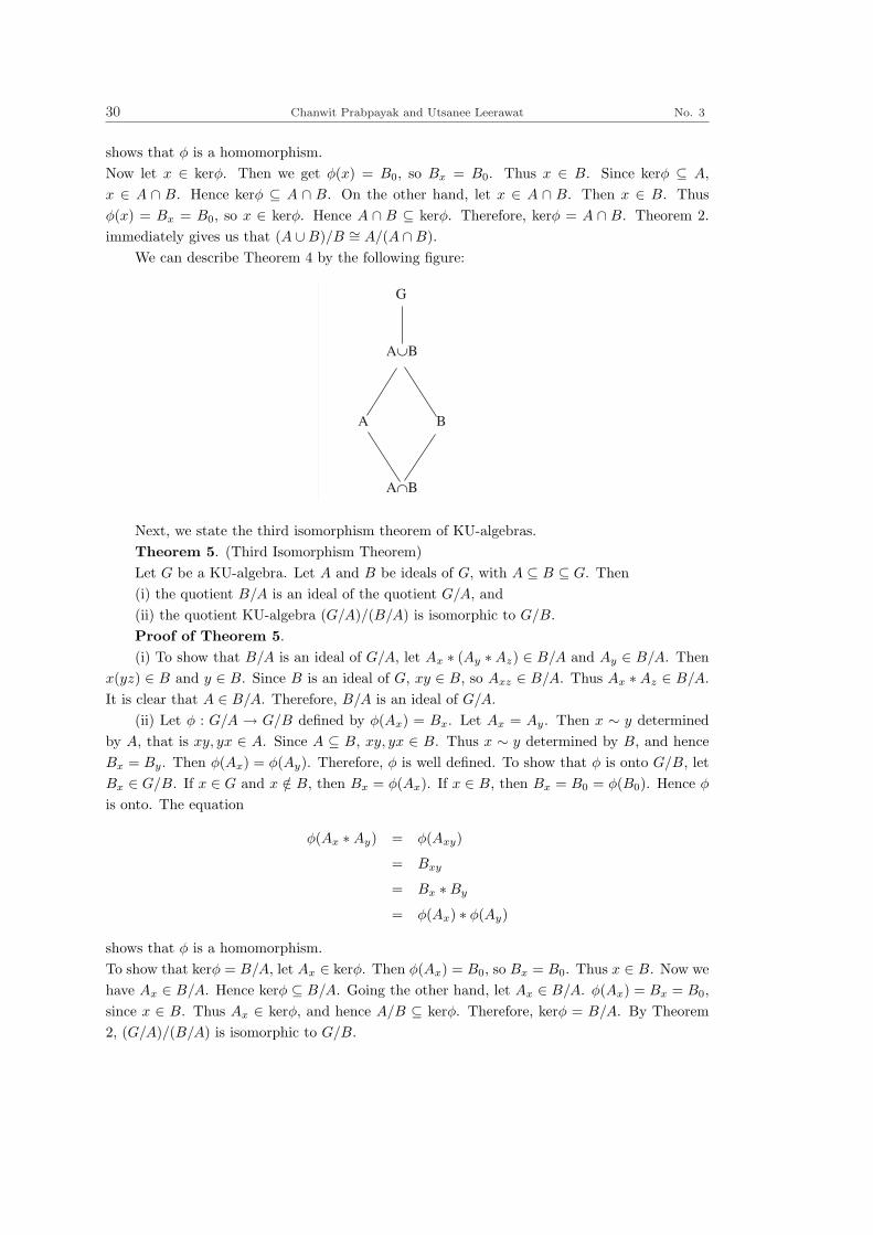
shows that φ is a homomorphism.Now let x ∈ kerφ. Then we get φ(x) = B0, so Bx = B0. Thus x ∈ B. Since kerφ ⊆ A,x ∈ A ∩ B. Hence kerφ ⊆ A ∩ B. On the other hand, let x ∈ A ∩ B. Then x ∈ B. Thusφ(x) = Bx = B0, so x ∈ kerφ. Hence A ∩ B ⊆ kerφ. Therefore, kerφ = A ∩ B. Theorem 2.immediately gives us that (A ∪B)/B ∼= A/(A ∩B).
We can describe Theorem 4 by the following figure:
A
A B
B
A!B
G
Next, we state the third isomorphism theorem of KU-algebras.Theorem 5. (Third Isomorphism Theorem)Let G be a KU-algebra. Let A and B be ideals of G, with A ⊆ B ⊆ G. Then(i) the quotient B/A is an ideal of the quotient G/A, and(ii) the quotient KU-algebra (G/A)/(B/A) is isomorphic to G/B.Proof of Theorem 5.(i) To show that B/A is an ideal of G/A, let Ax ∗ (Ay ∗ Az) ∈ B/A and Ay ∈ B/A. Then
x(yz) ∈ B and y ∈ B. Since B is an ideal of G, xy ∈ B, so Axz ∈ B/A. Thus Ax ∗ Az ∈ B/A.It is clear that A ∈ B/A. Therefore, B/A is an ideal of G/A.
(ii) Let φ : G/A → G/B defined by φ(Ax) = Bx. Let Ax = Ay. Then x ∼ y determinedby A, that is xy, yx ∈ A. Since A ⊆ B, xy, yx ∈ B. Thus x ∼ y determined by B, and henceBx = By. Then φ(Ax) = φ(Ay). Therefore, φ is well defined. To show that φ is onto G/B, letBx ∈ G/B. If x ∈ G and x /∈ B, then Bx = φ(Ax). If x ∈ B, then Bx = B0 = φ(B0). Hence φ
is onto. The equation
φ(Ax ∗Ay) = φ(Axy)
= Bxy
= Bx ∗By
= φ(Ax) ∗ φ(Ay)
shows that φ is a homomorphism.To show that kerφ = B/A, let Ax ∈ kerφ. Then φ(Ax) = B0, so Bx = B0. Thus x ∈ B. Now wehave Ax ∈ B/A. Hence kerφ ⊆ B/A. Going the other hand, let Ax ∈ B/A. φ(Ax) = Bx = B0,since x ∈ B. Thus Ax ∈ kerφ, and hence A/B ⊆ kerφ. Therefore, kerφ = B/A. By Theorem2, (G/A)/(B/A) is isomorphic to G/B.

Vol. 5 On Isomorphisms of KU-algebras 31
G/A
B/A
A/A
G
B
A
It turns out that an analogous result of the third isomorphism theorem for groups is alsotrue for KU-algebras.
References
[1] W.A. Dudek and X. Zhang, On ideals and congruences in BCC-algebras, CzechoslovakMath. Journal, 48(1998), No. 123, 21-29.
[2] W.A. Dudek, On proper BCC-algebras, Bull. Inst. Math. Academia Sinica, 20(1992),137-150.
[3] C. Prabpayak and U. Leerawat, On ideals and conguences in KU-algebras, ScientiaMagna Journal, 5(2009), No. 1, 54-57.

Scientia MagnaVol. 5 (2009), No. 3, 32-39
Smarandache friendly numbers-anotherapproach
S. M. Khairnar†, Anant W. Vyawahare‡ and J. N. Salunke]
†Departmrnt of Mathematics, Maharashtra Academy of Engineering, Alandi, Pune, India‡Gajanan Nagar, Wardha Road, Nagpur-440015, India
]Departmrnt of Mathematics, North Maharashtra University, Jalgoan, IndiaE-mail: [email protected] [email protected]
Abstract One approach to Smarandache friendly numbers is given by A.Murthy, who defined
them Ref [1]. Another approach is presented here.
Keywords Smarandache friendly numbers.
Smarandache friendly numbers were defined by A. Murthy [1] as follows.Definition 1. If the sum of any set of consecutive terms of a sequence is equal to the
product of first and last number, then the first and the last numbers are called a pair ofSmarandache friendly numbers.
Here, we will consider a sequence of natural numbers.1. It is easy to note that (3, 6) is a friendly pair as 3 + 4 + 5 + 6 = 18 = 3 · 6.2. By elementary operations and trial, we can find such pairs, but as magnitude of natural
numbers increases, this work becomes tedious. Hence an algorithm is presented here.Assume that (m,n) is a pair of friendly numbers, n > m, so that
m + (m + 1) + (m + 2) + · · ·+ n = m · n.
Let n = m + k, where k is a natural number. Then the above equation becomes
m + (m + 1) + (m + 2) + · · ·+ n = m · (m + k).
On simplification, this gives,
k2 + k − 2(m2 −m) = 0.
That is,
k =−1 +
√1 + 8(m2 −m)
2,
considering the positive sign only.Now, k will be a natural number only if 1+8(m2−m) is a perfect square of an odd natural
number.

Vol. 5 Smarandache friendly numbers-another approach 33
For m = 3, we have k = 3, so that n = 3 + 3 = 6, and then (3, 6) are friendly numbers aswe observed earlier.
For m = 5, k = −1+√
1612 , which is not an integer. Hence k does not exist for every m.
For m = 15, k = 20, hence n = 35. So the next pair of friendly numbers is (15, 35). Otherpairs are (85, 204) and (493, 1189).
At the end, the list of m and 1 + 8(m2 −m) is given using a computer software.
2. If (m,n) is a friendly pair, of natural numbers, then it is conjectured that (m+2n, 2m+5n− 1) is also a friendly pair.
Since, (3, 6) and (15, 35) are frendly pairs, we have 3x + 6y = 15 and 3p + 6q = 35, forsome x, y, p, q being natural numbers. These equations are true for x = 1, y = 2, p = 2andq = 5.With 1 to be substracted from second equation.
These solutions are unique, hence this conjecture.
This suggests that there are infinite pairs of friendly natural numbers.
Definition 2. [1] x and y are primes. They are called Smarandache friendly primes ifthe sum of any set of consecutive primes, whose first term is x and last is y, is equal to theirproduct x · y .
Example. (2, 5), (3, 13), (5, 31) are pairs of friendly primes, for 3 + 5 + 7 + 11 + 13 = 39 =3 · 13.
Since the primes are not uniformly distributed, an algorithm for friendly primes seems tobe impossible.
4. For various sequences, different pairs of friendly numbers can be obtained.
The values of m ≤ 1000 and 1 + 8(m2 −m) are given below. Those with perfect squaresare underlined. Only four pairs were obtained.
1 1.0000 2 4.1231 3 7.0000 4 9.8489 5 12.6886
6 15.5242 7 18.3576 8 21.1896 9 24.0208 10 26.8514
11 29.6816 12 32.5115 13 35.3412 14 38.1707 15 41.0000
16 43.8292 17 46.6583 18 49.4874 19 52.3163 20 55.1453
21 57.9741 22 60.8030 23 63.6318 24 66.4605 25 69.2892
26 72.1180 17 74.9466 28 77.7753 29 80.6040 30 83.4326
31 86.2612 32 89.0898 33 91.9184 34 94.7470 35 97.5756
36 100.4042 37 103.2327 38 106.0613 39 108.8899 40 111.7184
41 114.5469 42 117.3755 43 120.2040 44 123.0325 45 125.8610
46 128.6895 47 131.5181 48 134.3466 49 137.1751 50 140.0036
51 142.8321 52 145.6606 53 148.4891 54 151.3176 55 154.1460
56 156.9745 57 159.8030 58 162.6315 59 165.4600 60 168.2884
61 171.1169 62 173.9454 63 176.7739 64 179.6023 65 182.4308
66 185.2593 67 188.0877 68 190.9162 69 193.7447 70 196.5731

34 S. M. Khairnar, Anant W. Vyawahare and J. N. Salunke No. 3
71 199.4016 72 202.2301 73 205.0585 74 207.8870 75 210.7155
76 213.5439 77 216.3724 78 219.2008 79 222.0293 80 224.8577
81 227.6862 82 230.5146 83 233.3431 84 236.1716 85 239.0000
86 241.8284 87 244.6569 88 247.4854 89 250.3138 90 253.1423
91 255.9707 92 258.7992 93 261.6276 94 264.4561 95 267.2845
96 270.1129 97 272.9414 98 275.7698 99 278.5983 100 281.4267
101 284.2552 102 287.0836 103 289.9120 104 292.7405 105 295.5689
106 298.3974 107 301.2258 108 304.0543 109 306.8827 110 309.7112
111 312.5396 112 315.3680 113 318.1965 114 321.0249 115 323.8534
116 326.6818 117 329.5103 118 332.3387 119 335.1671 120 337.9956
121 340.8240 122 343.6524 123 346.4809 124 349.3093 125 352.1378
126 354.9662 127 357.7946 128 360.6231 129 363.4515 130 366.2799
131 369.1084 132 371.9368 133 374.7653 134 377.5937 135 380.4221
136 383.2506 137 386.0790 138 388.9074 139 391.7359 140 394.5643
141 397.3928 142 400.2212 143 403.0496 144 405.8781 145 408.7065
146 411.5349 147 414.3634 148 417.1918 149 420.0202 150 422.8487
151 425.6771 152 428.5056 153 431.3340 154 434.1624 155 436.9908
156 439.8193 157 442.6477 158 445.4761 159 448.3046 160 451.1330
161 453.9615 162 456.7899 163 459.6183 164 462.4467 165 465.2752
166 468.1036 167 470.9321 168 473.7605 169 476.5889 170 479.4174
171 482.2458 172 485.0742 173 487.9026 174 490.7311 175 493.5595
176 496.3879 177 499.2164 178 502.0448 179 504.8733 180 507.7017
181 510.5301 182 513.3585 183 516.1870 184 519.0154 185 521.8439
186 524.6723 187 527.5007 188 530.3292 189 533.1576 190 535.9860
191 538.8145 192 541.6429 193 544.4713 194 547.2997 195 550.1282
196 552.9566 197 555.7850 198 558.6135 199 561.4419 200 564.2703
201 567.0988 202 569.9272 203 572.7556 204 575.5840 205 578.4125
206 581.2409 207 584.0693 208 586.8978 209 589.7262 210 592.5546
211 595.3831 212 598.2115 213 601.0399 214 603.8683 215 606.6968
216 609.5252 217 612.3536 218 615.1821 219 618.0105 220 620.8389
221 623.6674 222 626.4958 223 629.3242 224 632.1526 225 634.9811
226 637.8095 227 640.6379 228 643.4664 229 646.2948 230 649.1232
231 651.9517 232 654.7801 233 657.6085 234 660.4370 235 663.2654
236 666.0938 237 668.9222 238 671.7507 239 674.5791 240 677.4075
241 680.2360 242 683.0644 243 685.8928 244 688.7213 245 691.5497
246 694.3781 247 697.2065 248 700.0350 249 702.8634 250 705.6918
251 708.5203 252 711.3487 253 714.1771 254 717.0056 255 719.8340
256 722.6624 257 725.4908 258 728.3193 259 731.1477 260 733.9761
261 736.8046 262 739.6330 263 742.4614 264 745.2899 265 748.1183
266 750.9467 267 753.7751 268 756.6036 269 759.4320 270 762.2604

Vol. 5 Smarandache friendly numbers-another approach 35
271 765.0889 272 767.9173 273 770.7457 274 73.5742
275 776.4026 276 779.2310 277 782.0594 278 784.8879
279 787.7163 280 790.5447 281 793.3732 282 796.2016
283 799.0300 284 801.8585 285 804.6869 286 807.5153
287 810.3438 288 813.1722 289 816.0006 290 818.8290
291 821.6575 292 824.4859 293 827.3143 294 830.1428
295 832.9712 296 835.7996 297 838.6281 298 841.4565
299 844.2849 300 847.1133 301 849.9418 302 852.7702
303 855.5986 304 858.4271 305 861.2555 306 864.0839
307 866.9124 308 869.7408 309 872.5692 310 875.3976
311 878.2261 312 881.0545 313 883.8829 314 886.7114
315 889.5398 316 892.3682 317 895.1967 318 898.0251
319 900.8535 320 903.6819 321 906.5103 322 909.3387
323 912.1672 324 914.9956 325 917.8240 326 920.6525
327 923.4809 328 926.3093 329 929.1378 330 931.9662
331 934.7946 332 937.6230 333 940.4515 334 943.2799
335 946.1083 336 948.9368 337 951.7652 338 954.5936
339 957.4221 340 960.2505 341 963.0789 342 965.9073
343 968.7358 344 971.5642 345 974.3926 346 977.2211
347 980.0495 348 982.8779 349 985.7064 350 988.5348
351 991.3632 352 994.1917 353 997.0201 354 999.8485
355 1002.6769 356 1005.5054 357 1008.3338 358 1011.1622
359 1013.9907 360 1016.8190 361 1019.6475 362 1022.4759
363 1025.3043 364 1028.1328 365 1030.9612 366 1033.7897
367 1036.6180 368 1039.4465 369 1042.2749 370 1045.1034
371 1047.9318 372 1050.7603 373 1053.5886 374 1056.4171
375 1059.2455 376 1062.0740 377 1064.9023 378 1067.7307
379 1070.5592 380 1073.3876 381 1076.2161 382 1079.0444
383 1081.8729 384 1084.7013 385 1087.5298 386 1090.3582
387 1093.1866 388 1096.0150 389 1098.8435 390 1101.6719
391 1104.5004 392 1107.3287 393 1110.1572 394 1112.9856
395 1115.8141 396 1118.6425 397 1121.4709 398 1124.2993
399 1127.1278 400 1129.9562 401 1132.7847 402 1135.6130
403 1138.4415 404 1141.2699 405 1144.0984 406 1146.9268
407 1149.7552 408 1152.5836 409 1155.4120 410 1158.2405
411 1161.0688 412 1163.8973 413 1166.7257 414 1169.5542
415 1172.3826 416 1175.2111 417 1178.0394 418 1180.8679
419 1183.6963 420 1186.5248 421 1189.3531 422 1192.1816
423 1195.0100 424 1197.8385 425 1200.6669 426 1203.4954
427 1206.3237 428 1209.1522 429 1211.9806 430 1214.8091

36 S. M. Khairnar, Anant W. Vyawahare and J. N. Salunke No. 3
431 1217.6375 432 1220.4659 433 1223.2943 434 1226.1228
435 1228.9512 436 1231.7797 437 1234.6080 438 1237.4365
439 1240.2649 440 1243.0933 441 1245.9218 442 1248.7501
443 1251.5786 444 1254.4070 445 1257.2355 446 1260.0638
447 1262.8923 448 1265.7207 449 1268.5492 450 1271.3776
451 1274.2061 452 1277.0344 453 1279.8629 454 1282.6913
455 1285.5198 456 1288.3481 457 1291.1766 458 1294.0050
459 1296.8335 460 1299.6619 461 1302.4904 462 1305.3187
463 1308.1472 464 1310.9756 465 1313.8041 466 1316.6324
467 1319.4608 468 1322.2893 469 1325.1177 470 1327.9462
471 1330.7745 472 1333.6030 473 1336.4314 474 1339.2599
475 1342.0883 476 1344.9167 477 1347.7451 478 1350.5736
479 1353.4020 480 1356.2305 481 1359.0588 482 1361.8873
483 1364.7157 484 1367.5442 485 1370.3726 486 1373.2010
487 1376.0294 488 1378.8579 489 1381.6863 490 1384.5148
491 1387.3431 492 1390.1716 493 1393.0000 494 1395.8284
495 1398.6569 496 1401.4852 497 1404.3137 498 1407.1421
499 1409.9706 500 1412.7990 501 1415.6274 502 1418.4558
503 1421.2843 504 1424.1127 505 1426.9412 506 1429.7695
507 1432.5980 508 1435.4264 509 1438.2549 510 1441.0833
511 1443.9117 512 1446.7401 513 1449.5686 514 1452.3970
515 1455.2255 516 1458.0538 517 1460.8823 518 1463.7107
519 1466.5391 520 1469.3676 521 1472.1959 522 1475.0244
523 1477.8528 524 1480.6813 525 1483.5096 526 1486.3381
527 1489.1665 528 1491.9950 529 1494.8234 530 1497.6519
531 1500.4802 532 1503.3087 533 1506.1371 534 1508.9656
535 1511.7939 536 1514.6224 537 1517.4508 538 1520.2793
539 1523.1077 540 1525.9362 541 1528.7645 542 1531.5930
543 1534.4214 544 1537.2499 545 1540.0782 546 1542.9066
547 1545.7351 548 1548.5635 549 1551.3920 550 1554.2203
551 1557.0488 552 1559.8772 553 1562.7057 554 1565.5341
555 1568.3625 556 1571.1909 557 1574.0194 558 1576.8478
559 1579.6763 560 1582.5046 561 1585.3331 562 1588.1615
563 1590.9900 564 1593.8184 565 1596.6469 566 1599.4752
567 1602.3037 568 1605.1321 569 1607.9604 570 1610.7889
571 1613.6173 572 1616.4458 573 1619.2742 574 1622.1027
575 1624.9310 576 1627.7595 577 1630.5879 578 1633.4164
579 1636.2448 580 1639.0732 581 1641.9016 582 1644.7301
583 1647.5585 584 1650.3870 585 1653.2153 586 1656.0438
587 1658.8722 588 1661.7007 589 1664.5291 590 1667.3575

Vol. 5 Smarandache friendly numbers-another approach 37
591 1670.1859 592 1673.0144 593 1675.8428 594 1678.6711
595 1681.4996 596 1684.3280 597 1687.1565 598 1689.9849
599 1692.8134 600 1695.6417 601 1698.4702 602 1701.2986
603 1704.1271 604 1706.9554 605 1709.7839 606 1712.6123
607 1715.4408 608 1718.2692 609 1721.0977 610 1723.9260
611 1726.7545 612 1729.5829 613 1732.4114 614 1735.2397
615 1738.0682 616 1740.8966 617 1743.7250 618 1746.5535
619 1749.3818 620 1752.2103 621 1755.0387 622 1757.8672
623 1760.6956 624 1763.5240 625 1766.3524 626 1769.1809
627 1772.0093 628 1774.8378 629 1777.6661 630 1780.4946
631 1783.3230 632 1786.1515 633 1788.9799 634 1791.8083
635 1794.6367 636 1797.4652 637 1800.2936 638 1803.1221
639 1805.9504 640 1808.7789 641 1811.6073 642 1814.4357
643 1817.2642 644 1820.0925 645 1822.9210 646 1825.7494
647 1828.5779 648 1831.4063 649 1834.2347 650 1837.0631
651 1839.8916 652 1842.7200 653 1845.5485 654 1848.3768
655 1851.2053 656 1854.0337 657 1856.8622 658 1859.6906
659 1862.5190 660 1865.3474 661 1868.1759 662 1871.0043
663 1873.8328 664 1876.6611 665 1879.4895 666 1882.3180
667 1885.1464 668 1887.9749 669 1890.8032 670 1893.6317
671 1896.4601 672 1899.2886 673 1902.1169 674 1904.9454
675 1907.7738 676 1910.6023 677 1913.4307 678 1916.2592
679 1919.0875 680 1921.9160 681 1924.7444 682 1927.5729
683 1930.4012 684 1933.2297 685 1936.0581 686 1938.8866
687 1941.7150 688 1944.5433 689 1947.3718 690 1950.2002
691 1953.0287 692 1955.8571 693 1958.6855 694 1961.5139
695 1964.3424 696 1967.1708 697 1969.9993 698 1972.8276
699 1975.6561 700 1978.4845 701 1981.3130 702 1984.1414
703 1986.9698 704 1989.7982 705 1992.6267 706 1995.4551
707 1998.2836 708 2001.1119 709 2003.9403 710 2006.7688
711 2009.5972 712 2012.4257 713 2015.2540 714 2018.0825
715 2020.9109 716 2023.7394 717 2026.5677 718 2029.3962
719 2032.2246 720 2035.0531 721 2037.8815 722 2040.7100
723 2043.5383 724 2046.3668 725 2049.1953 726 2052.0237
727 2054.8521 728 2057.6804 729 2060.5090 730 2063.3374
731 2066.1658 732 2068.9941 733 2071.8225 734 2074.6511
735 2077.4795 736 2080.3079 737 2083.1362 738 2085.9648
739 2088.7932 740 2091.6216 741 2094.4500 742 2097.2786
743 2100.1069 744 2102.9353 745 2105.7637 746 2108.5923
747 2111.4207 748 2114.2490 749 2117.0774 750 2119.9060
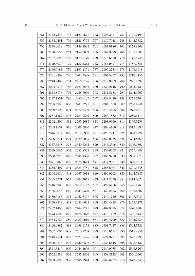
38 S. M. Khairnar, Anant W. Vyawahare and J. N. Salunke No. 3
751 2122.7344 752 2125.5627 753 2128.3911 754 2131.2195
755 2134.0481 756 2136.8765 757 2139.7048 758 2142.5332
759 2145.3618 760 2148.1902 761 2151.0186 762 2153.8469
763 2156.6755 764 2159.5039 765 2162.3323 766 2165.1606
767 2167.9893 768 2170.8176 769 2173.6460 770 2176.4744
771 2179.3030 772 2182.1313 773 2184.9597 774 2187.7881
775 2190.6167 776 2193.4451 777 2196.2734 778 2199.1018
779 2201.9302 780 2204.7588 781 2207.5872 782 2210.4155
783 2213.2439 784 2216.0725 785 2218.9009 786 2221.7292
787 2224.5576 788 2227.3862 789 2230.2146 790 2233.0430
791 2235.8713 792 2238.7000 793 2241.5283 794 2244.3567
795 2247.1851 796 2250.0137 797 2252.8420 798 2255.6704
799 2258.4988 800 2261.3271 801 2264.1558 802 2266.9841
803 2269.8125 804 2272.6409 805 2275.4695 806 2278.2979
807 2281.1262 808 2283.9546 809 2286.7832 810 2289.6116
811 2292.4399 812 2295.2683 813 2298.0969 814 2300.9253
815 2303.7537 816 2306.5820 817 2309.4106 818 2312.2390
819 2315.0674 820 2317.8958 821 2320.7241 822 2323.5527
823 2326.3811 824 2329.2095 825 2332.0378 826 2334.8665
827 2337.6948 828 2340.5232 829 2343.3516 830 2346.1802
831 2349.0085 832 2351.8369 833 2354.6653 834 2357.4939
835 2360.3223 836 2363.1506 837 2365.9790 838 2368.8076
839 2371.6360 840 2374.4644 841 2377.2927 842 2380.1211
843 2382.9497 844 2385.7781 845 2388.6064 846 2391.4348
847 2394.2634 848 2397.0918 849 2399.9202 850 2402.7485
851 2405.5771 852 2408.4055 853 2411.2339 854 2414.0623
855 2416.8909 856 2419.7192 857 2422.5476 858 2425.3760
859 2428.2046 860 2431.0330 861 2433.8613 862 2436.6897
863 2439.5183 864 2442.3467 865 2445.1750 866 2448.0034
867 2450.8318 868 2453.6604 869 2456.4888 870 2459.3171
871 2462.1455 872 2464.9741 873 2467.8025 874 2470.6309
875 2473.4592 876 2476.2878 877 2479.1162 878 2481.9446
879 2484.7729 880 2487.6016 881 2490.4299 882 2493.2583
883 2496.0867 884 2498.9153 885 2501.7437 886 2504.5720
887 2507.4004 888 2510.2288 889 2513.0574 890 2515.8857
891 2518.7141 892 2521.5425 893 2524.3711 894 2527.1995
895 2530.0278 896 2532.8562 897 2535.6848 898 2538.5132
899 2541.3416 900 2544.1699 901 2546.9985 902 2549.8269
903 2552.6553 904 2555.4836 905 2558.3123 906 2561.1406
907 2563.9690 908 2566.7974 909 2569.6257 910 2572.4543

Vol. 5 Smarandache friendly numbers-another approach 39
911 2575.2827 912 2578.1111 913 2580.9395 914 2583.7681
915 2586.5964 916 2589.4248 917 2592.2532 918 2595.0818
919 2597.9102 920 2600.7385 921 2603.5669 922 2606.3955
923 2609.2239 924 2612.0522 925 2614.8806 926 2617.7092
927 2620.5376 928 2623.3660 929 2626.1943 930 2629.0227
931 2631.8513 932 2634.6797 933 2637.5081 934 2640.3364
935 2643.1650 936 2645.9934 937 2648.8218 938 2651.6501
939 2654.4788 940 2657.3071 941 2660.1355 942 2662.9639
943 2665.7925 944 2668.6208 945 2671.4492 946 2674.2776
947 2677.1062 948 2679.9346 949 2682.7629 950 2685.5913
951 2688.4197 952 2691.2483 953 2694.0767 954 2696.9050
955 2699.7334 956 2702.5620 957 2705.3904 958 2708.2188
959 2711.0471 960 2713.8757 961 2716.7041 962 2719.5325
963 2722.3608 964 2725.1895 965 2728.0178 966 2730.8462
967 2733.6746 968 2736.5032 969 2739.3315 970 2742.1599
971 2744.9883 972 2747.8167 973 2750.6453 974 2753.4736
975 2756.3020 976 2759.1304 977 2761.9590 978 2764.7874
979 2767.6157 980 2770.4441 981 2773.2727 982 2776.1011
983 2778.9294 984 2781.7578 985 2784.5864 986 2787.4148
987 2790.2432 988 2793.0715 989 2795.9001 990 2798.7285
991 2801.5569 992 2804.3853 993 2807.2136 994 2810.0422
995 2812.8706 996 2815.6990 997 2818.5273 998 2821.3560
999 2824.1843 1000 2827.0127
References
[1] Amarnath Murthy, Some Notions on Least Common Multiples, Smarandache NotionsJournal, Vol. 12(2001), 307-308.

Scientia MagnaVol. 5 (2009), No. 3, 40-43
Simple closed null curves in Minkowski 3-Space
Emin Ozyılmaz†, Suha Yılmaz‡ and Suur Nizamoglu‡
† Department of Mathematics, Faculty of Science, Ege University,Bornova-Izmir, Turkey
‡ Department of Mathematics, Buca Educational Faculty, Dokuz Eylul University,35160 Buca-Izmir, Turkey
E-mail: [email protected] [email protected]
Abstract In this work, we present some characterizations of simple closed null curves in
Minkowski 3-space. Moreover, in the same space, we study a special case of such curves “Null
curves of constant breadth”.
Keywords Minkowski 3-Space, simple closed null curve, curves of constant breadth.
§1. Introduction
At the beginning of the twentieth century, A. Einstein’s theory opened a door to newgeometries such as Minkowski space, which is simultaneously the geometry of special relativityand the geometry induced on each fixed tangent space of an arbitrary Lorentzian manifold.
In recent years, the theory of degenerate submanifolds has been treated by researchersand some classical differential geometry topics have been extended to Lorentz manifolds. Forinstance, in [6] and [10], the authors studied space-like and time-like curves of constant breadthin Minkowski 3-space, respectively. These studies have been treated based of the papers [1],[3], [8] and [9], in the spaces E2, E3 and E4.
In this work, we investigate position vector of a simple closed null curve and give somecharacterizations in Minkowski space E3
1 . Additionally, we express a characterization in thecase of constant breadth.
§2. Preliminaries
To meet the requirements in the next sections, here, the basic elements of the theory ofcurves in the space E3
1 are briefly presented (A more complete elementary treatment can befound in [2]).
The Minkowski 3-space E31 is the Euclidean 3-space E3 provided with the standard flat
metric given by

Vol. 5 Simple Closed Null Curves in Minkowski 3-Space 41
g = −dx21 + dx2
2 + dx23,
where (x1, x2, x3) is a rectangular coordinate system of E31 . Since g is an indefinite metric,
recall that a vector v ∈ E31 can have one of three Lorentzian characters: it can be space-like if
g(v, v) > 0 or v = 0, time-like if g(v, v) < 0 and null if g(v, v) = 0 and v 6= 0. Similarly, anarbitrary curve ϕ = ϕ(s) in E3
1 can locally be space-like, time-like or null (light-like), if all of itsvelocity vectors ϕ′ are respectively space-like, time-like or null (light-like), for every s ∈ I ⊂ R.The pseudo-norm of an arbitrary vector a ∈ E3
1 is given by ‖a‖ =√|g(a, a)|. ϕ is called an
unit speed curve if velocity vector v of ϕ satisfies ‖v‖ = 1. For vectors v, w ∈ E31 it is said to
be orthogonal if and only if g(v, w) = 0.
Denote by T,N, B the moving Frenet frame along the curve ϕ in the space E31 . For an
arbitrary curve ϕ with first and second curvature, κ and τ in the space E31 , the following Frenet
formulae are given in [4]:
If ϕ is a null curve, then the Frenet formulae has the form
T ′
N ′
B′
=
0 κ 0
τ 0 −κ
0 −τ 0
T
N
B
, (1)
satisfying equations
g(T, T ) = g(B,B) = g(T, N) = g(N, B) = 0,g(N, N) = 1, g(T,B) = 1.
In this case, κ can take only two values: κ = 0 when α is a null straight line, or κ = 1 in allother cases.
Recall that an arbitrary curve is called a W−curve if it has constant Frenet curvatures [7].In the rest of the paper, we shall assume κ = 1 at every point.
§3. Simple closed null curves in Minkowski 3-Space
Let ϕ = ϕ(s) be null curve in the space E31 . Moreover, let us suppose ϕ = ϕ(s) simple
closed null curve in the space E31 . These curves will be denoted by (C). The normal plane
at every point P on the curve meets the curve at a single point Q other than P . We call thepoint Q the opposite point of P . We consider a curve in the class Γ as in [5] having paralleltangents T and T ∗ in opposite directions at the opposite points ϕ and ϕ∗ of the curve. Here,we suppose both ϕ and ϕ∗ are unit speed null curves of E3
1 . A simple closed null curve havingparallel tangents in opposite directions at opposite points can be represented with respect toFrenet frame by the equation
ϕ∗ = ϕ + λT + µN + δB. (2)

42 Emin Ozyılmaz, Suha Yılmaz and Suur Nizamoglu No. 3
where λ, µ and δ are arbitrary functions of s and ϕ and ϕ∗ are opposite points. Differentiatingboth sides of (2) and considering Frenet equations, we have
dϕ∗
ds= T ∗ =
dλ
ds+ µτ + 1
T +
dµ
ds+ λ− δτ
N +
dδ
ds− µ
B. (3)
We know that T ∗ = −T . Then, we get the following system of ordinary differential equations:
λ′ = −µτ − 2
µ′ = δτ − λ
δ′ = µ
. (4)
Using system (4), we have the following differential equation with respect to λ as
d
ds
1τ
d
ds
[1τ
(dλ
ds+ 2
)]− d
ds
(λ
τ
)− 1
τ
(dλ
ds+ 2
)= 0. (5)
Theorem 3.1. This obtained differential equation of third order with variable coefficients(5) is a characterization for the simple closed null curve in E3
1 . Via its solution, position vectorof ϕ∗ can be determined.
However, a general solution of (5) has not yet been found. Let us suppose ϕ = ϕ(s) be anull W−curve in the space E3
1 . In this case the differential equation (5) transforms to
d3λ
ds3− 2τ
dλ
ds− 2τ = 0. (6)
According to signature of τ , we study the following cases.Case 3.1. τ > 0. Then, we have the solution of the differential equation (6) as
λ = Φ1 cosh√
2τs + Φ2 sinh√
2τs− s (7)
where Φ1,Φ2 ∈ R. Thus, we may express other components, respectively,
µ = −√
2τ
(Φ1 sinh
√2τs + Φ2 cosh
√2τs +
1√2τ
)(8)
andδ = −1
τ
(Φ1 cosh
√2τs + Φ2 sinh
√2τs− s
). (9)
Case 3.2. τ < 0. In this case, we have the solution
λ = Ψ1 cos√−2τs + Ψ2 sin
√−2τs− s (10)
for the real numbers Ψ1,Ψ2 ∈ R. Since, we write other components
µ = −1τ
√−2τ
(−Φ1 sin
√−2τs + Φ2 cos√−2τs +
1√−2τ
)(11)
andδ = −1
τ
(Ψ1 cos
√−2τs + Ψ2 sin√−2τs− s
). (12)
Theorem 3.2. Position vector of a simple closed null W−curve in Minkowski space E31 can
be composed by the components (7), (8) and (9); or (10), (11) and (12) according to singatureof the torsion.

Vol. 5 Simple Closed Null Curves in Minkowski 3-Space 43
§4. Null curves of constant breadth in Minkowski 3-Space
In this section, we give a characterization of the null curves of constant breadth in Minkowski3-space.
Let us suppose the null curve treated in the previous section has constant breadth. Inanother words, let the distance between opposite points of C and C∗ be constant. Then, dueto null frame vectors, we may express
‖ϕ∗ − ϕ‖ = 2λδ + µ2 = l2 = constant. (13)
Differentiating both sides of (13), we immediately arrive
δdλ
ds+ λ
dδ
ds+ µ
dµ
ds= 0. (14)
Considering system of ordinary differential equations (4), we have
δ = 0 (15)
and, thereafterλ = µ = 0. (16)
Since, we give:Theorem 4.1. There does not exist null curves of constant breadth in Minkowski 3-space
E31 .
References
[1] A. Magden and O. Kose, On The Curves of Constant Breadth, Tr. J. of Mathematics,1(1997), 277-284.
[2] B. O’Neill, Semi-Riemannian Geometry, Academic Press, New York, 1983.[3] L. Euler, De Curvis Trangularibis, Acta Acad. Petropol, 1780, 3-30.[4] K. Ilarslan and O. Boyacıoglu, Position vectors of a timelike and a null helix in
Minkowski 3-space, Chaos, Solitons and Fractals, 2008.[5] M. Fujivara, On Space Curves of Constant Breadth, Tohoku Math. J., 5(1914), 179-184.[6] M. Onder, H. Kocayigit and O. Kılıc, Spacelike curves of Constant Breadth in Minkowski
3-space, Paper presented, VI. National Geometry Syposium, Uludag University, 1-4 July ofBursa, Turkey, 2008.
[7] M. Petrovic-Torgasev and E. Sucurovic, W -curves in Minkowski space-time, Novi SadJ. Math., 32(2002), No. 2, 55-65.
[8] O. Kose, Some Properties of Ovals and Curves of Constant Width in a Plane, DogaMat., 2(1984), No. 8, 119-126.
[9] O. Kose, On Space Curves of Constant Breadth, Doga Math., 1(1986), No. 10, 11-14.[10] S. Yılmaz and M. Turgut, On the Time-like curves of Constant Breadth in Minkowski
3-space., International J.Math. Combin., 3(2008), 34-39.

Scientia MagnaVol. 5 (2009), No. 3, 44-48
On the Elliptic cylindrical Tzitzeica curves inMinkowski 3-Space
Murat Kemal Karacan† and Bahaddin Bukcu‡
†Department of Mathematics, Usak University, Usak, 64200, Turkey‡Department of Mathematics, Gazi Osman Pasa University, Tokat, Turkey
E-mail: [email protected]
Abstract Elliptic cylindrical curves satisfying Tzitzeica condition are obtained via the
solution of the forced harmonic equation in Minkowski 3-Space. In addition, we have given
the conditions to be of spacelike, timelike and null curve of the elliptic cylindrical Tzitzeica
curve.
Keywords Tzitzeica curve, Elliptic cylindrical curve, Minkowski 3-Space.
§1. Preliminaries and Introduction
The Minkowski 3-space E31 is the Euclidean 3-space E3 provided with the Lorentzian inner
product〈x, y〉L = x1y1 + x2y2 − x3y3,
where x = (x1, x2, x3) and y = (y1, y2, y3). An arbitrary vector x = (x1, x2, x3) in E31can have
one of three Lorentzian causal characters: it is spacelike if 〈x, x〉L > 0 or x = 0, timelike if〈x, x〉L < 0 and null (lightlike) if 〈x, x〉L = 0 and x 6= 0. Similarly, an arbitrary curve α = α(s)in E3
1 is locally spacelike, timelike or null (lightlike), if all of its velocity vectors (tangents)α′(s) = T (s) are respectively spacelike, timelike or null, for each s ∈ I ⊂ IR. Lorentzianvectoral product of x and y is defined by
x ∧L y = (x2y3 − x3y2, x3y1 − x1y3, x2y1 − x1y2) .
Recall that the pseudo-norm of an arbitrary vector x ∈ E31 is given by ‖x‖L =
√|〈x, x〉L|. Ifthe curve α is non-unit speed, then
κ(t) =
∥∥∥α′(t) ∧L α
′′(t)
∥∥∥L∥∥∥α
′(t)
∥∥∥3
L
, τ(t) =det
(α′(t), α
′′(t), α
′′′(t)
)
∥∥∥α′(t) ∧L α
′′(t)
∥∥∥2
L
. (1.1)
If the curve α is unit speed, then
κ(s) = ‖α′′(s)‖L , τ(s) = ‖B′(s)‖L . (1.2)
[1,4].In this paper we have interested in Tzitzeica elliptic cylindrical curves in Minkowski 3-
Space, more precisely we ask in what conditions a cylindrical curve is a Tzitzeica one, namely

Vol. 5 On the Elliptic cylindrical Tzitzeica curves in Minkowski 3-Space 45
the function t → τ(t)d2(t) is constant, where d(t) is the distance from origin to the osculating plane
of curve. The Tzitzeica condition yields a third-order ODE which in our framework admits adirect integration. Therefore the final answer of main problem is given via a second order ODEwhich in the elliptic case is exactly the equation of a forced harmonic oscillator. In this case,the solution depends of four real constants: one defining the Tzitzeica condition and other threeobtained by integration.
§2. Elliptic Cylindrical Tzitzeica curves in Minkowski 3-
Space
Proposition 1. Let α(t) be an elliptic cylindrical curve in Minkowski 3-Space.Then, thecurve α(t) is Tzitzeica curve if and only if
f(t) = f(0) cos t + f ′(0) sin t +
t∫
0
sin(u− t)Ku + c
du,
where f(0), f ′(0), K 6= 0 and c are real constants.Proof. Let in E3
1 a curve C given in vectorial form C : α = α(t). This curve is calledelliptic cylindrical if has the expression
α(t) = (cos t, sin t, f(t)) (2.1)
and differentiation of α(t), we have
α′(t) = (− sin t, cos t, f ′(t))
α′′(t) = (− cos t,− sin t, f ′′(t)) (2.2)
α′′′(t) = (sin t,− cos t, f ′′(t))
for some f ∈ C∞(R). From Eq.(1.1) and Eq.(2.2), the torsion function is
τ(t) =det (α′, α′′, α′′′)‖α′ ∧L α′′‖2L
=f ′ + f ′′′
f ′2 + f ′′2 − 1.
Then the distance from origin to the osculating plane is
d(t) =|f + f ′′|√
|f ′2 + f ′′2 − 1| .
Let us suppose that the curve is Tzitzeica with the constant K 6= 0, because the curve is notcontained in a plane
K(t) =τ(t)d2(t)
=f ′ + f ′′′
f ′2 + f ′′2 − 1
∣∣f ′2 + f ′′2 − 1∣∣2
|f + f ′′|2
=f ′(t) + f ′′′(t)
(f(t) + f ′′(t))2.

46 Murat Kemal Karacan and Bahaddin Bukcu No. 3
Integration gives
f ′′(t) + f(t) = − 1Kt + c
, (2.3)
where c is a real constant. Then the Laplace transform gives[s2Y (s)− sf(0)− f ′(0)
]+ Y (s) = −L G(t) = −g(s),
where Y (s) and G(s) denote the Laplace transform of f(t) and g(t) respectively, and f(0) andf ′(0) are arbitrary constants. Hence
Y (s) = f(0)s
s2 + 1+ f ′(0)
1s2 + 1
− 1s2 + 1
L G(t)
= f(0)s
s2 + 1+ f ′(0)
1s2 + 1
− 1s2 + 1
g(s)
and thereforef(t) = f(0) cos t + f ′(0) sin t− sin(t) ∗G(t),
where the function denoted by sin(t) ∗G(t) and defined as
sin(t) ∗G(t) =
t∫
0
G(u) sin(u− t)du
is called the convolution of the functions sin t and G(t) or
f(t) = f(0) cos t + f ′(0) sin t +
t∫
0
G(u) sin(u− t)du.
Theorem 1. Let α(t) be elliptic cylindrical Tzitzeica curve, then the curve α(t) are space-like, timelike and null curve if and only if f ′2(0) < 1, f ′2(0) > 1 and f ′2(0) = 1, respectively.
Proof. Since the curve α(t) = (cos t, sin t, f(t)), the tangent of the curve is T = α′(t) =(− sin t, cos t, f ′(t)). The taylor series of the function f in the neighbourhood of zero is
f(t) = f(0)− f ′(0)t +f ′′(0)
2!t2 +
f ′′′(0)3!
t3 + · · ·
We take into consideration satisfying
f(0) = f ′(0) 6= 0, 0 = f ′′(0) = f ′′′(0) = · · · (2.4)
in the neighbourhood of zero. Then we have
f(0) cos t + f ′(0) sin t +
t∫
0
sin(u− t)Ku + c
du = f(0) + f ′(0)t.
From the last equation, we get
f(0) cos t = f(0),
f ′(0) sin t = f ′(0)t,t∫
0
sin(u− t)Ku + c
du = 0.

Vol. 5 On the Elliptic cylindrical Tzitzeica curves in Minkowski 3-Space 47
Then, for t → 0
cos t = 1,
sin t = t,
Limt→0
t∫
0
sin(u− t)Ku + c
du = 0.
Thus, satisfying Eq.(2.4) as t → 0 , sin t = t and the function f is written such as
f(t) = f ′(0) sin t.
If we take derivative of the last equation for t and square, we have
f ′2(t) = f ′2(0) cos2 t,
〈T (t), T (t)〉L = 1− f ′2 > 0,
or
(f ′)2 (t) < 1,
(f ′)2 (0) cos2 t < 1.
Since |cos t| < 1, from the last equation, we have(i) The curve α(t) is spacelike curve if and only if
〈T (t), T (t)〉L = 1− f ′2 > 0.
Then, we have(f ′)2 (0) < 1.
(ii) The Tzitzeica curve α(t) is timelike curve if and only if
〈T (t), T (t)〉L = 1− f ′2 < 0.
Then, we havef ′2(0) > 1.
(iii) The Tzitzeica curve α(t) is null curve if and only if
〈T (t), T (t)〉L = 1− f ′2 = 0.
Then, we havef ′2(0) = 1.
References
[1] Akyıldız, E., Akyıldız, Y., Alpay, S., Erkip, A. and Yazıcı, A., Lecture Notes on Differ-ential Equations, Metu Publications, 1981, 293.

48 Murat Kemal Karacan and Bahaddin Bukcu No. 3
[2] Bukcu, B., Karacan, M. K., On the involute and evolute curves of the spacelike curvewith a spacelike binormal in Minkowski 3-space, Int. J.of Contemp. Math. Sci., 2(2007), No.5-8.
[3] Crasmareanu, M., Cylindrical Tzitzeica Curves Implies Forced Harmonic, Oscillators,Balkan Journal of Geometry and Its Applications, 7(2002), No. 1, 37-42.
[4] Petrovic-Torgasev, M., Sucurovic, E., Some Characterizations of The Spacelike, TheTimelike and The Null Curves on The Pseudohyperbolic Space H2
0 in E31 , Kragujevac J.Math.,
22(2000), 71-82.[5] Ross, S.L., Differential Equation, John Wiley & Sons, Inc, New York, 1984.

Scientia MagnaVol. 5 (2009), No. 3, 49-55
On n-Frechet spaces
Nguyen Van Dung † and Vo Thi Le Hang ‡
Mathematics Faculty, Dongthap University, Caolanh City, Dongthap Province, Vietnam
E-mail: [email protected] [email protected]
Abstract In this paper, we introduce the notion of n-sequential closure operators and use
these operators to construct classes of n-Frechet spaces as generalizations of the class of Frechet
spaces. Then we get some necessary and sufficiency conditions for a sequential space to be a
Frechet space. These results are generalizations of the preceding one of W. C. Hong in [5].
Keywords Frechet, n-Frechet, sequential, sequential closure, n-sequential closure.
§1. Introduction and results
M. Venkataraman poses the following problem in [8].Problem 1.1. Characterize “the class of topological spaces which can be specified com-
pletely by knowledge of their convergent sequences”.It is well known and useful fact that every first-countable space falls into this class. To
solve Problem 1.1, S. P. Franklin introduced notions of Frechet spaces and sequential spaces([1], [2] and [3]). Recently, W. C. Hong has investigated the relation between Frechet spacesand sequential spaces under the sequential closure operator c1 [4],
c1(A) =x ∈ X : there exists a sequence xn : n ∈ N ⊂ A, xn → x
,
for all subset A of X.Recall the following notions.Definition 1.2. ([2], [7]) Let (X, c) be a topological space endowed with the closure
operator c.(1) X is a Frechet space, if for all A ⊂ X, c(A) = c1(A).(2) X is a sequential space, if for all A ⊂ X, A = c(A) whenever A = c1(A).(3) X has countable tightness, if for all A ⊂ X, x ∈ c(C) for some countable subset C of
A whenever x ∈ c(A).From the fact that the closure operator of Frechet spaces is specified completely by knowl-
edge of their convergent sequences, it is natural to ask whether we can generalize the class ofFrechet spaces under this property. That is, we are interested by the following question.
Question 1.3. Is there a class of spaces which contains properly the class of Frechet spacessuch that the closure operator of spaces in this class is specified completely by knowledge oftheir convergent sequences?
1This work is Supported in part by the Natural Science Foundation of PUD (No T0 05/06).
50 Nguyen Van Dung and Vo Thi Le Hang No. 3
In this paper, we introduce the notion of n-sequential closure operators cn, n ∈ N, anduse these operators to give classes of n-Frechet spaces as generalizations of the class of Frechetspaces. Then, we answer affirmatively Question 1.3. As the application, we give necessary andsufficiency conditions for a sequential space to be a Frechet space. These results are generationsof the preceding one of W. C. Hong in [5].
Assume that all spaces are Hausdorff, all maps are continuous and onto, N denotes the setof all natural numbers, and ω denotes N ∪ 0. For terms which are not defined here, pleaserefer to [1].
§2. Frechet spaces
In this section we recall some results on Frechet spaces.Proposition 2.1. ([1], Theorem 1.6.14). Every first-countable space is a Frechet space
and every Frechet space is a sequential space.Proposition 2.2. ([7]). Ever sequential space has countable tightness.Definition 2.3. ([1]). Let f : X −→ Y be a map.(1) f is a pseudo-open map, if y ∈ intf(U) whenever f−1(y) ⊂ U with U open in X.(2) f is a quotient map, if U open in Y whenever f−1(U) open in X.Example 2.4. There exists a sequential space without being Frechet.Proof. Recall the Arens’ space S2 [6]. Let T0 = an : n ∈ N be a sequence converging
to a 6∈ T0, and Tn, n ∈ N, be a sequence converging to bn 6∈ Tn. Put T =⊕
n∈N(Tn ∪ bn).Then S2 = a ∪ (
⋃n∈ω Tn) is a quotient space of (T0 ∪ a)⊕ T by identifying each bn ∈ T to
an ∈ T0. We get that S2 is a sequential space without being Frechet.Proposition 2.5. ([2], Proposition 2.1).(1) Every subspace of a Frechet space is a Frechet space.(2) The disjoint topological sum of any family of Frechet spaces is a Frechet space.Proposition 2.6. ([2], Proposition 2.3). Let f : X −→ Y be a quotient map from a
Frechet space X onto Y . Then f is pseudo-open if and only if Y is Frechet.Corollary 2.7. Frechet spaces are preserved by pseudo-open maps, particularly, by closed
or open maps.Proposition 2.8. ([3], Proposition 7.2 ). A sequential space is Frechet if and only if it is
hereditarily sequential.Example 2.9. ([3], Example 7.4). The product of two Frechet spaces can be sequential
without being Frechet.Proposition 2.10. ([5], Theorem 2). A sequential space X is Frechet if and only if
c1(A) = c(A) for every countable subset A of X.Proposition 2.11. ([2], Proposition 2.4) Every Frechet space is precisely the pseudo-open
image of a topological sum of convergent sequences.Corollary 2.12. The following are equivalent for a space X.(1) X is a Frechet space,(2) X is a pseudo-open image of a locally compact metric space,(3) X is a pseudo-open image of a locally separable metric space,

Vol. 5 On n-Frechet spaces 51
(4) X is a pseudo-open image of a metric space.
§3. n-Frechet spaces
Definition 3.1. Let (X, c) be a topological endowed with the closure operator c. A mapcn, n ∈ N, n ≥ 2, defines by induction on n:
cn(A) = c1(c(n−1)(A)),
for all A ⊂ X to be called an n-sequential closure operator. The sequential closure operator c1
is also called an 1-sequential closure operator for convince.Proposition 3.2. Let (X, c) be a topological endowed with the closure operator c. Then
the following hold for all n ∈ N.(1) cn(∅) = ∅.(2) A ⊂ c1(A) ⊂ · · · ⊂ cn(A) ⊂ c(A) for all A ⊂ X.(3) cn(A) ⊂ cn(B) for all A ⊂ B ⊂ X.(4) cn(A ∪B) = cn(A) ∪ cn(B) for all A,B ⊂ X.Definition 3.3. Let (X, c) be a topological space endowed with the closure operator c,
and n ∈ N. Then X is called an n-Frechet space, if c(A) = cn(A) for all A ⊂ X.Remark 3.4. (1) An 1-Frechet space is precisely a Frechet space.(2) By Proposition 3.2, cn(A) ⊂ c(A) for all A ⊂ X. Then, to prove that X is an n-Frechet,
it suffices to show that c(A) ⊂ cn(A) for all A ⊂ X.Next, we construct i-spaces and i-sequences by induction on i ∈ N to consider the relation
between n-Frechet spaces.Definition 3.5. Let X be a topological space.(1) X is called an 1-space, if X = x ∪ xn : n ∈ N with xn → x 6∈ xn : n ∈ N, and all
xn’s being distinct. Here xn, n ∈ N, is called a 0-limit point of X, and x is called an 1-limitpoint of X.
(2) For each i ∈ N, i ≥ 2, X is called an i-space, if X = x ∪ (⋃
n∈ω Xn) is a quotientspace obtained from a topological sum (X0 ∪ x) ⊕
( ⊕n∈N(Xn ∪ xn)
)by identifying each
yn ∈ Xn to xn ∈ X0, where Xn, n ∈ N, is an (i − 1)-space with an (i − 1)-limit point yn, andX0 = x ∪ xn : n ∈ N is an 1-space with an 1-limit point x. Here x is called an i-limit pointof X, and a j-limit point of Xn’s, j = 0, . . . , i− 1, is called a j-limit point of X.
Remark 3.6. (1) Each 1-space is an infinite convergent sequence, and each 2-space is anAren’s space S2 (see Example 2.4).
(2) For each i ∈ N, an i-space is an infinite countable set.Definition 3.7. Let X be a topological space and S ⊂ X.(1) S is called an 1-sequence of X, if S = xn : n ∈ N is a sequence converging to x. We
say that S converges under 1 to x, and write S1→ x, here x is called an 1-limit point of S.
(2) For i ∈ N, i ≥ 2, S is called an i-sequence of X, if S =⋃
n∈N Ln, where Ln is an
(i − 1)-sequence, Lni−1→ xn for each n ∈ N, and L0 = xn : n ∈ N is an 1-sequence with
L01→ x. We say that S converges under i to x, and write S
i→ x, here x is called an i-limitpoint of S.

52 Nguyen Van Dung and Vo Thi Le Hang No. 3
Remark 3.8. The following hold.(1) The set S of all 0-limit points of an i-space X is an i-sequence satisfying that ci(S) = X.(2) Each i-sequence is a countable set.(3) Every finite set is an i-sequence. But the following Example 3.9 proves that there is an
infinite countable subset of a metric space without being an i-sequence.Example 3.9. There is an infinite countable subset of a metric space without being an
i-sequence.Proof. Let R be a discrete space. Then R is a metric space. We have that N is an infinite
countable subset of R, and N is not an i-sequence. In fact, if there exists an i ∈ N such that Nis an i-sequence. Since each 1-sequence of R with the discrete topology is finite, N is finite. Itis a contradiction.
Lemma 3.10. Let X be a topological space, and A ⊂ X. Then x ∈ cn(A) if and only ifthere exists an n-sequence S ⊂ A such that S
n→ x.Proof. Necessity. For n = 1, we get that x ∈ c1(A). Then there exists a sequence
S = xn : n ∈ N ⊂ A, xn → x. It is clear that S is an 1-sequence, S ⊂ A, and S1→ x.
For each n ≥ 2, we get that x ∈ cn(A) = c1(c(n−1)(A)). Then there exists an 1-sequence
L ⊂ c(n−1)(A) such that L1→ x. Put L = xi : i ∈ N then xi ∈ c(n−1)(A) for all i ∈ N.
Note that for each i ∈ N, there is an (n − 1)-sequence Li ⊂ A such that Lin−1→ xi. Then
S =⋃
i∈N Li ⊂ A is an n-sequence, and Sn→ x.
Sufficiency. Since Sn→ x, x ∈ cn(S). By Proposition 3.2, x ∈ cn(A)
Corollary 3.11. Let X be an n-Frechet space, and A ⊂ X. Then x ∈ c(A) if and only ifthere exists an n-sequence S ⊂ A such that S
n→ x.Proposition 3.12. The following hold for a space X.(1) If X is an n-Frechet space, then X is an (n + 1)-Frechet space.(2) If X be an n-Frechet space, then X is a sequential space.Proof. (1) Let A ⊂ X and x ∈ c(A). Since X is n-Frechet, x ∈ cn(A). Note that
cn(A) ⊂ c(n+1)(A). Then x ∈ c(n+1)(A). So c(A) ⊂ c(n+1)(A), i.e., X is an (n + 1)-Frechetspace.
(2) Let A ⊂ X and A = c1(A). We need to prove that A = c(A). It follows from A = c1(A)that A = c1(A) = ... = c(n−1)(A) = cn(A). Since c(A) = cn(A), A = c(A).
Corollary 3.13. Every n-Frechet space has countable tightness.The following examples to prove that inverse implications in Proposition 3.12 do not hold.Example 3.14. For all n ∈ N, there exists an (n + 1)-Frechet space which is not an
n-Frechet space.Proof. For each n ∈ N, let X be an (n + 1)-space.(i) X is an (n + 1)-Frechet space.Let A ⊂ X and x ∈ c(A). We shall prove that x ∈ c(n+1)(A).If x is a 0-limit point, then x is an isolated point. Then from x ∈ c(A) we get x ∈ A ⊂
c(n+1)(A).If x is an 1-limit point, then x has a countable neighborhood system. Then from x ∈ c(A)
we get that there exists a sequence xn : n ∈ N ⊂ A such that xn → x. Hence x ∈ c1(A) ⊂c(n+1)(A).

Vol. 5 On n-Frechet spaces 53
If x is an i-limit point, i = 2, . . . , n + 1, then there exist (i− 1)-spaces Ym’s, m ∈ N, with(i − 1)-limit points ym’s, and an 1-sequence Y0 = ym : m ∈ N with the 1-limit point x suchthat x∪ (
⋃n∈ω Yn) ⊂ X, and x∪ (
⋃m∈ω Ym) is an i-space. Sice x ∈ c(A), there is infinitely
numbers m ∈ N such that A ∩ Ym is an (i− 1)-sequence with the (i− 1)-limit point ym. Thenthere is infinitely numbers m such that ym ∈ c(i−1)(A∩ Ym). Hence x ∈ ci(A∩ Ym) ⊂ ci(A). Itimplies that x ∈ ci(A) ⊂ c(n+1)(A).
(ii) X is not an n-Frechet space.Let
A = x ∈ X : x is the 0-limit point of X.
Then cn(A) = X − a with a is the (n + 1)-limit point of X. On the other hand, a ∈ c(A).Therefore cn(A) 6= c(A). So X is not n-Frechet.
Example 3.15. There is a sequential space which is not an n-Frechet space for all n ∈ N.Proof. Let S∞ = ⊕m∈NSm, where Sm’s are m-spaces.(i) S∞ is a sequential space.It follows from the proof of Example 3.14 that each m-space Sm is an m-Frechet space.
Then each Sm is a sequential space by Proposition 3.12. So S∞ is a sequential space by ([2],Proposition 1.6).
(ii) S∞ is not an n-Frechet space.For each n ∈ N, we put
A =x ∈ S(n+1) : x is the 0-limit point of S(n+1)
.
Then cn(A) = S(n+1) − x, here x is the (n + 1)-limit point of S(n+1). On the other hand,x ∈ c(A). Then c(A) 6= cn(A). It implies that S∞ is not an n-Frechet space.
Remark 3.16. It follows from Proposition 3.12, Example 3.14, and Example 3.15 that
Frechet ⇒ n-Frechet ⇒ (n + 1)-Frechet ⇒ sequential,
for all n ∈ N. Moreover, all of inverse implications do not hold if n ≥ 2.Lemma 3.17. Let f : X −→ Y be a map. If S is an n-sequence in X with the n-limit
point x, then f(S) is an n-sequence in Y with the n-limit point f(x).Proposition 3.18. Let f : X −→ Y be a map and X be an n-Frechet space, then Y is
an n-Frechet space.Proof. For all A ⊂ Y and y ∈ c(A), we shall prove that y ∈ cn(A). Suppose that
f−1(y) ∩ c(f−1(A)
)= ∅. Then U = X − c
(f−1(A)
)is an open set containing f−1(y). Since
f is a pseudo-open map and f−1(y) ⊂ U , y ∈ int(f(U)
)= int
(f(X − c
(f−1(A)
))= int
(Y −
f(c(f−1(A)
))) ⊂ int(Y −A) = Y − c(A). So y 6∈ c(A). It is a contradiction. Then there exists
some point x ∈ f−1(y) ∩ c(f−1(A)
). Since X is an n-Frechet space, there is an n-sequence
S ⊂ f−1(A) such that Sn→ x by Corollary 3.11. On the other hand, y = f(x) is the n-limit
point of n-sequence f(S) ⊂ f(f−1(A)
)= A by Lemma 3.17. It implies that y ∈ cn(A).
Example 3.19. For all n ≥ 2, there exists an n-Frechet space without being hereditarilyn-Frechet.

54 Nguyen Van Dung and Vo Thi Le Hang No. 3
Proof. For n ≥ 2, let X be an n-space. Then X is an n-Frechet space by the proof ofExample 3.14. We shall prove that X is not hereditarily n-Frechet. Conversely, suppose that X
is hereditarily n-Frechet. By Proposition 3.12, X is a hereditarily sequential space. It followsfrom Proposition 2.8 that X is an 1-Frechet space. It is a contradiction (see Example 3.14).Then X is not hereditarily n-Frechet.
Proposition 3.20. Every closed subspace of an n-Frechet space is an n-Frechet space.Proof. Let X be an n-Frechet space, Y ⊂ X, Y = c(Y ) and A ⊂ Y . Let cY and cY
n bethe closure operator and the n-sequential closure operator of the subspace Y , respectively. Weneed to prove that cY (A) = cY
n (A). Since cn(A) = c(A) ⊂ c(Y ) = Y , cn(A) = cYn (A). On the
other hand, cY (A) = c(A) ∩ Y = c(A) ∩ c(Y ) = c(A) = cn(A). Then cY (A) = cYn (A).
Proposition 3.21. The disjoint topological sum of any family of n-Frechet spaces is ann-Frechet space.
Proof. Let Xi : i ∈ I be a disjoint collection of n-Frechet spaces, and X =⊕
i∈I Xi.For any A ⊂ X and x ∈ c(A), we need to prove that x ∈ cn(A). Since x ∈ c(A), there existssome i ∈ I such that x ∈ c(A) ∩ Xi. Then x ∈ cXi(A) = cXi
n (A), here cXi and cXin are the
closure operator and n-sequential closure operator of Xi, respectively. Since cXin (A) ⊂ cn(A),
x ∈ cn(A).Proposition 3.22. A space having the countable tightness X is an n-Frechet space if and
only if c(A) = cn(A) for every countable subset A ⊂ X.Proof. Necessary. It is clear.Sufficiency. Let cn(A) = c(A) for every countable subset A ⊂ X. For any B ⊂ X we need
to prove that c(B) = cn(B). For any x ∈ c(B), since X has the countable tightness, there isa countable subset C ⊂ B such that x ∈ c(C). Note that c(C) = cn(C) by countability of C.Then x ∈ cn(C) ⊂ cn(B). It implies that c(B) = cn(B).
Corollary 3.23. The following hold for a space X.(1) Under X being a sequential space, then X is an n-Frechet space if and only if c(A) =
cn(A) for every countable subset A ⊂ X.(2) Under X being an m-Frechet space and m > n, then X is an n-Frechet space if and
only if cm(A) = cn(A) for every countable subset A ⊂ X.Proof. It is straightforward from Proposition 2.2, Corollary 3.13, and Proposition 3.22.Remark 3.24. For n = 1 in Corollary 3.23.(1) we get ([5], Theorem 2). Then, Proposition
3.22 is a generation of ([5], Theorem 2) (see Proposition 2.10).Proposition 3.25. A sequential space X is an n-Frechet space if and only if cn(S) =
c(n+1)(S) for every (n + 1)-sequence S ⊂ X.Proof. Necessary. It is straightforward from Proposition 3.21.Sufficiency. Conversely, suppose that X is not n-Frechet. Then there exists A ⊂ X such
that cn(A) 6= c(A). Since A ⊂ cn(A) ⊂ c(A), c(A) ⊂ c(cn(A)
) ⊂ c(c(A)
). Then c
(cn(A)
)=
c(A). It implies that cn(A) is not closed in a sequential space X. So cn(A) 6= c1
(cn(A)
). Hence
there is some x ∈ c1
(cn(A)
)such that x 6∈ cn(A). Because x ∈ c1
(cn(A)
)= c(n+1)(A), there is
an (n + 1)-sequence S ⊂ A such that Sn+1→ x by Lemma 3.10. Then x ∈ c(n+1)(S) = cn(S) ⊂
cn(A). It implies that x ∈ cn(A). It is a contradiction.Corollary 3.26. A sequential space X is an 1-Frechet space if and only if c1(S) = c2(S)

Vol. 5 On n-Frechet spaces 55
for every 2-sequence S ⊂ X.Corollary 3.27. A space X is an 1-Frechet space if and only if c1(S) = c(S) for every
2-sequence S ⊂ X.Proof. Necessary. It is obvious.Sufficiency. It follows from Proposition 3.2 that c1(S) = c2(S). Then X is an 1-Frechet
space by Corollary 3.26.Remark 3.28. It follows from Example 3.9 that the collection of n-sequences is a proper
subset of the collection of countable subsets of a sequential space (indeed, a metric space). So,Corollary 3.27 and Corollary 3.26, are generations of ([5], Theorem 2) (see Proposition 2.10).
It is well known that the product of a collection of Frechet spaces is not Frechet (seeExample 2.9). So the following question rises naturally.
Question 3.29. Is the product of a collection of n-Frechet spaces an n-Frechet space?Note that the answer of Question 3.29 is negative with Hausdorff assumption (see [1,2.3
K]).On the other hand, every Frechet space and sequential space is precisely the pseudo-open
image and the quotient image of a metric space, respectively (see Corollary 2.12 and ([2],Corollary 1.14), and the class of n-Frechet spaces is between the class of Frechet spaces theclass of sequential spaces (see Remark 3.16). So we have the following question.
Question 3.30. What maps is every n-Frechet space precisely image of a metric spaceunder?
References
[1] R. Engelking, General topology, Sigma series in pure mathematics, Heldermann Verlag,Berlin, 6(1988).
[2] S. P. Franklin,Spaces in which sequences suffic, Fund. Math., 57(1965), 107-115.[3] S. P. Franklin, Spaces in which sequences suffice II, Fund. Math., 61(1967), 51-56.[4] W. C. Hong, Some properties of the sequential closure operator on a generalized topo-
logical spaces, Comm. Korean Math. Soc., 13(1998), No. 2, 359-365.[5] W. C. Hong, On sequential spaces and a related class of spaces, Kyungpook Math.
Jour., 40(2000), 149-155.[6] S. Lin, A note on the Arens’ space and sequential fan, Topology Appl., 81(1997),
185-196.[7] Y. Tanaka, Theory of k-networks II, Questions Answers in Gen. Topology, 19(2001),
27-46.[8] M. Venkataraman, Directed sets in topology, Math. Student, 30(1962), 99-100.

Scientia MagnaVol. 5 (2009), No. 3, 56-59
Product of powers of quasinormal compositionoperators
K. Thirugnanasambandam† and S. Panayappan ‡
† Department of Mathematics, Sri Ramakrishna Engineering College,Coimbatore-641 022, India
‡ Department of Mathematics,Chikkanna Government Arts College, Tiruppur, IndiaE-mail: [email protected] [email protected]
Abstract Let Ti, i = 1, 2 be measurable transformations which define bounded composition
operators CTi on L2 of a σ-finite measure space. Denote their respective Radon-Nikodym
derivatives by hi, i = 1, 2. The main result of the paper is that, if hi Ti = hj a.e.,
for i, j = 1, 2, then for each of the positive integers m, n, p the operators (CmT1Cn
T2)p and
(CmT2Cn
T1)p are quasinormal. As a consequence, we see that the sufficient condition established
in our paper [5] for quasinormality of a composition operator is actually sufficient for all
powers to be quasinormal.
Keywords Quasinormal operators, powers of quasinormal composition operators.
§1. Preliminaries
Let (X, Σ, λ) be a sigma-finite measure space and let T be a measurable transformationfrom X into itself. Set L2 = L2(X, Σ, λ). The equation CT f = f T for every f ∈ L2 defines acomposition transformation from L2 to the space of C-valued functions on X. CT is a boundedlinear operator on L2 precisely when (i) λ T−1 is absolutely continuous with respect to λ and(ii) h = d(λ T−1)/dλ is in L∞(X, Σ, λ) = L∞. Denote by R(CT ) the range of CT , by C∗Tthe adjoint of CT , and define T−1(Σ) as the relative completion of the σ - algebra T−1(A):A ∈ Σ.
The following lemmas, due to Harrington and Whitley[2], is well known and useful.Lemma 1.1. Let P denotes the projection of L2 onto R(CT ).
(i) C∗T CT f = hf and CT C∗T f = (h T )Pf, for all f ∈ L2. (1)(ii) R(CT ) = f ∈ L2 : f is T−1(Σ) measurable . (2)(iii) If f is T−1(Σ) measurable and g and fg belongs to L2, then P (fg) = fP (g). (3)
Lemma 1.2. With h, T and P as above,
< (hn T )Pg, g >=< (hn T )g, g >, n ∈ N, g ∈ L2.
Let B(H) denote the Banach algebra of all bounded linear operators on a Hilbert spaceH. An operator A on a complex Hilbert space H is said to be quasinormal if A commutes withA∗A.

Vol. 5 Product of powers of quasinormal composition operators 57
Theorem 1.3. Let CT , Mθ ∈ B(L2(λ)). Then CT Mθ = MθCT if and only if θ = θ T
a.e., where Mθ is the multiplication operator induced by θ.
Theorem 1.4. Let CT1 , CT2 ∈ B(L2(λ)) be quasinormal with h1T2 = h2 a.e. Then theproducts CT1CT2 and CT2 , CT1 are quasinormal.
§2. Main result and corollaries
In order to prove our main result, it is necessary to state and prove several lemmas. Theyare stated so that each lemma depends on some subset of the previously stated ones. Theproofs which are given conatin the essential ideas and may easily be adjusted to give the oneswe omit.
Lemma 2.1. If h T = h a.e., then for n ∈ N , f ∈ L2, we have< hnf, f >=< (Cn
T )∗CnT f, f >. (4)
Proof. For n = 1, the lemma is true by (1). Suppose (4) holds for n = 1, 2, · · · k and allf ∈ L2. Then < hkf, f >=< (Ck
T )∗CkT f, f >.
By induction hypothesis, < hk+1f, f >=< C∗T CT (C∗T CT )kf, f >
= < hhkf, f >=< (C∗T CT )k+1f, f >,
so that (4) holds for n = k + 1 and lemma 2.1 follows by induction.
Lemma 2.2. If h T = h a.e. , then for all n ∈ N , f ∈ L2, we have< Cn
T (CnT )∗f, f >=< (h T )nf, f >=< hnf, f >.
Proof. For n = 1, < CT C∗T f, f >=< (h T )f, f >=< hf, f > .
Since < C∗T CT f, f >=< (h T )Pf, f >=∫
(h T )|f |2dm
=∫
h |f|2 dm = < hf, f >.
Since hT = h a.e. By induction hypothesis we can prove lemma 2.2.
Now set A = CT1 , B = CT2 , so that the product AB is the operator CT3 .
Lemma 2.3. With A,B, h1 and h2 as above, if (a) h2 T2 = h1 a.e. (b) h1 T1 = h1 a.e.,then for each m,n ∈ N, f ∈ L2, we have < (AmBn)∗(AmBn)f, f >=< hm+n
2 f, f >.
Proof. First we proveClaim 2.3.1. With T and h as in §1, for all r,m ∈ N , f ∈ L2,we have < (h T )rCm
T f, CmT f >=< hr+mf, f >. (5)
Proof of claim 2.3.1.Fix r and induct on m. For m = 1, f ∈ L2
< (h T )rCT f, CT f >=∫
(h T )r(|f |2 T )dm
=∫
(hr|f |2)hdm =< hr+1f, f >.Suppose (5) holds for m = k and for all f ∈ L2.Then < (h T )rCk+1
T f, Ck+1T f >=< (h T )r+kCT f, CT f >
=∫
(hr+k T )(|f |2 T )dm =< hr+k+1f, f >.So (5) holds for m = k + 1. The claim 2.3.1. is proved by induction.To finish the proof of lemma 2.3, observe that< (AmBn)∗(AmBn)f, f >=< (Am)∗AmBnf,Bnf >
= < hm1 Bnf,Bnf) (by Lemma 2.1)

58 K.Thirugnanasambandam and S. Panayappan No. 3
= < (h2 T2)mBnf,Bnf) > (by hypothesis)= < hm+n
2 f, f > ( by claim 2.3.1)Lemma 2.4. With A,B, h1 and h2 as above, if hi Ti = hj , i, j = 1, 2, (6)
then for each m,n ∈ N, f ∈ L2, we have < (AmBn)(AmBn)∗f, f >=< hm+n2 f, f >.
Proof. First we proveClaim 2.4.1. If h T = h a.e., then for all r,m ∈ N, f ∈ L2, we have< hr(Cm
T )∗f, (CmT )∗f >=< (h T )r+mf, f >.
Proof of claim. Fix r and induct on m. For m = 1 and f ∈ L2,< hrC∗T f, C∗T f >=< (h T )rCT C∗T f, f >
= < (hr+1 T )Pf, f > ( by lemma 1.1)= < ((hr+1 T )f, f > ( by lemma 1.2)
By induction hypothesis claim 2.4.1 can be proved.Now < (AmBn) (AmBn)∗ f, f > = < [Bn(Bn)∗](Am)∗f, (Am)∗f >
= < (h2 T2)n(Am)∗f, (Am)∗f > (by lemma 2.2 )= < hn
1 (Am)∗f, (Am)∗f > (by hypothesis)= < (h1 T1)m+nf, f > (by claim 2.4.1)= < hm+n
2 f, f > (by hypothesis)Finally, similar technique and the above lemmas may be used to prove the following pair
of results, which we collect as Lemma 2.5 and state without proof.
Lemma 2.5. If (6) holds, then for all m,n, p ∈ N, f ∈ L2, we have
< [(AmBn)p]∗[(AmBn)p]f, f >=< h(m+n)p2 f, f > (7)
and< (AmBn)p[(AmBn)p]∗f, f >=< h
(m+n)p2 f, f > . (8)
Remark. h2 T2 = h2 is not necessary in the proof of (7). Now we may easily prove ourmain result.
Lemma 2.6. Let CT ∈ B(L2(λ)) be quasinormal. Then Mnh CT = CT Mn
h , n ∈N.Lemma 2.7. Let CTi
, CTjare quasinormal with hi Tj = hi a.e., hj Ti = hj a.e. Then
Mmhi
CnTj
= CnTj
Mmhi
.In this section, we shall show that the sufficient condition established in the Theorem
2.2[5] for quasinormality of a composition operator is actually sufficient for all powers to bequasinormal.
Theorem 2.8. Let CTibe quasinormal with hi Tj = hi a.e. for i, j = 1, 2. Then
(CmT1
CnT2
)p and (CmT2
CnT1
)p are also quasinormal for all m,n, p ∈ N.
Proof.Now(Cm
T1Cn
T2)((Cm
T1Cn
T2))∗(Cm
T1Cn
T2) = Cm
T1Cn
T2Cn∗
T2((Cm∗
T1Cm
T1)Cn
T2
= CmT1
CnT2
Cn∗T2
Mmh1
CnT2

Vol. 5 Product of powers of quasinormal composition operators 59
= CmT1
CnT2
(Cn∗T2
CnT2
)Mmh1
=CmT1
CnT2
Mnh2
Mmh1
=CmT1
Mnh2
CnT2
Mmh1
=Mnh2
CmT1
CnT2
Mmh1
=Cn∗T2
CnT2
CmT1
CnT2
Mmh1
=Cn∗T2
CnT2
CmT1
Mmh1
CnT2
=Cn∗T2
CnT2
Mmh1
CmT1
CnT2
=Cn∗T2
Mmh1
CnT2
CmT1
CnT2
=Cn∗T2
Cm∗T1
CmT1
CnT2
CmT1
CnT2
=(CmT1
CnT2
))∗(CmT1
CnT2
)(CmT1
CnT2
).
This implies CmT1
CnT2
is a quasinormal composition operator. And similarly CnT2
CmT1
is a quasi-normal composition operator.Therefore (Cm
T1Cn
T2)p and (Cm
T2Cn
T1)p are also quasinormal composition operators.
References
[1] P. R. Halmos, A Hilbert space problem book, Van Nostrand, Princeton, N. J., 1976.[2] D. J. Harrington and R. Whitley, Seminormal Composition Operators, J. Operator
Theory, 11(1984), 125-135.[3] A. Lambert, Hyponormal Composition Operators, Bull. London Math. Soc., 18(1986),
395-400.[4] E. Nordgren, Composition Operators in Hilbert space, Hilbert Space Operators, Lecture
notes in Math. Springer-Verlag, Berlin, 693(1978), 37-63.[5] S. Panayappan, D. Senthilkumar and K. Thirugnanasambandam, A Note on p-hyponormal
and product of quasinormal composition operators, Int. J. Math. Analysis, 3(2009), No. 1,49-54.
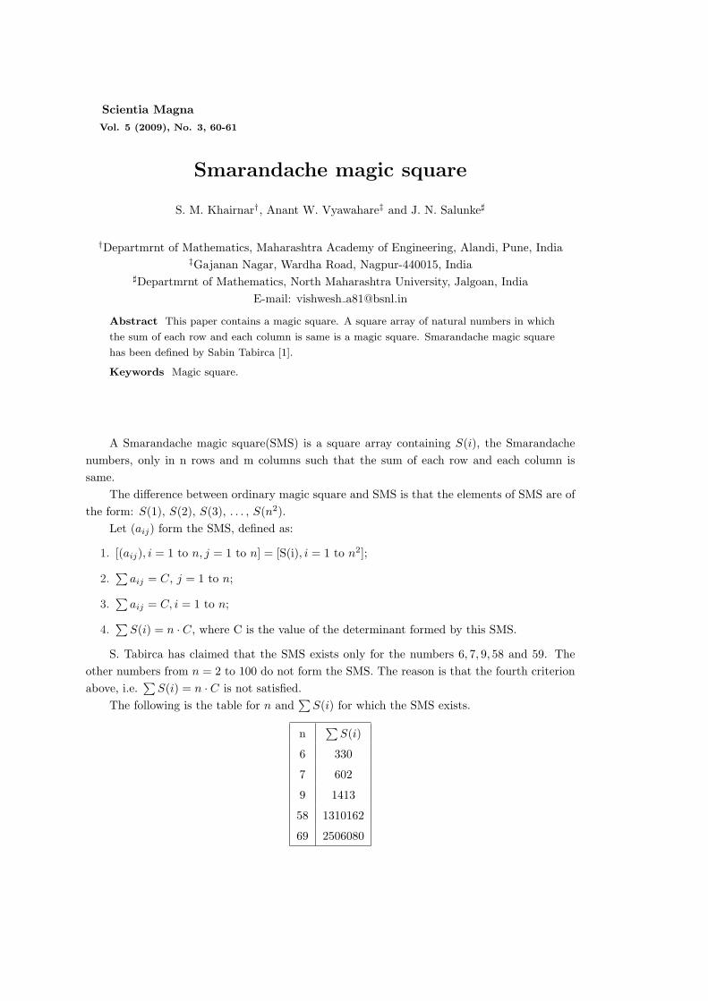
Scientia MagnaVol. 5 (2009), No. 3, 60-61
Smarandache magic square
S. M. Khairnar†, Anant W. Vyawahare‡ and J. N. Salunke]
†Departmrnt of Mathematics, Maharashtra Academy of Engineering, Alandi, Pune, India‡Gajanan Nagar, Wardha Road, Nagpur-440015, India
]Departmrnt of Mathematics, North Maharashtra University, Jalgoan, IndiaE-mail: vishwesh [email protected]
Abstract This paper contains a magic square. A square array of natural numbers in which
the sum of each row and each column is same is a magic square. Smarandache magic square
has been defined by Sabin Tabirca [1].
Keywords Magic square.
A Smarandache magic square(SMS) is a square array containing S(i), the Smarandachenumbers, only in n rows and m columns such that the sum of each row and each column issame.
The difference between ordinary magic square and SMS is that the elements of SMS are ofthe form: S(1), S(2), S(3), . . . , S(n2).
Let (aij) form the SMS, defined as:
1. [(aij), i = 1 to n, j = 1 to n] = [S(i), i = 1 to n2];
2.∑
aij = C, j = 1 to n;
3.∑
aij = C, i = 1 to n;
4.∑
S(i) = n · C, where C is the value of the determinant formed by this SMS.
S. Tabirca has claimed that the SMS exists only for the numbers 6, 7, 9, 58 and 59. Theother numbers from n = 2 to 100 do not form the SMS. The reason is that the fourth criterionabove, i.e.
∑S(i) = n · C is not satisfied.
The following is the table for n and∑
S(i) for which the SMS exists.
n∑
S(i)
6 330
7 602
9 1413
58 1310162
69 2506080

Vol. 5 Smarandache magic square 61
SMS does not exist for n = 2, 4, 5 . . . because for n = 4,∑
S(i), for i = 1 to 16 is 85, and4 does not divide 85. Similarly for other values of n.
Here is an example of Smarandache magic square. It is of order 6.
Sum of row elements
3 4 11 11 23 3 55
5 29 5 4 5 7 55
4 13 11 9 5 13 55
5 2 17 6 6 19 55
7 7 7 17 10 7 55
31 0 4 8 6 6 55
Sum of column elements 55 55 55 55 55 55 330
Now following is the magic square in the form of Smarandache functions.
S(3) S(4) S(11) S(22) S(23) S(6)
S(5) S(29) S(10) S(8) S(15) S(7)
S(12) S(13) S(33) S(27) S(20) S(26)
S(30) S(2) S(17) S(18) S(36) S(19)
S(14) S(21) S(35) S(34) S(25) S(28)
S(31) S(1) S(24) S(23) S(16) S(9)
Here,36∑
i=1
S(i) = 330, n = 6 and K =Value of each row/ column of magic square = 55, and
330 = 6× 55. Hence the condition36∑
i=1
S(i) = n.K is satisfied.
Therefore the above square is Smarandache magic square.
References
[1] Sabin Tabirca, Smarandache Magic Squares, Smarandache Notions Journal, Vol. 10(1999),100-104.
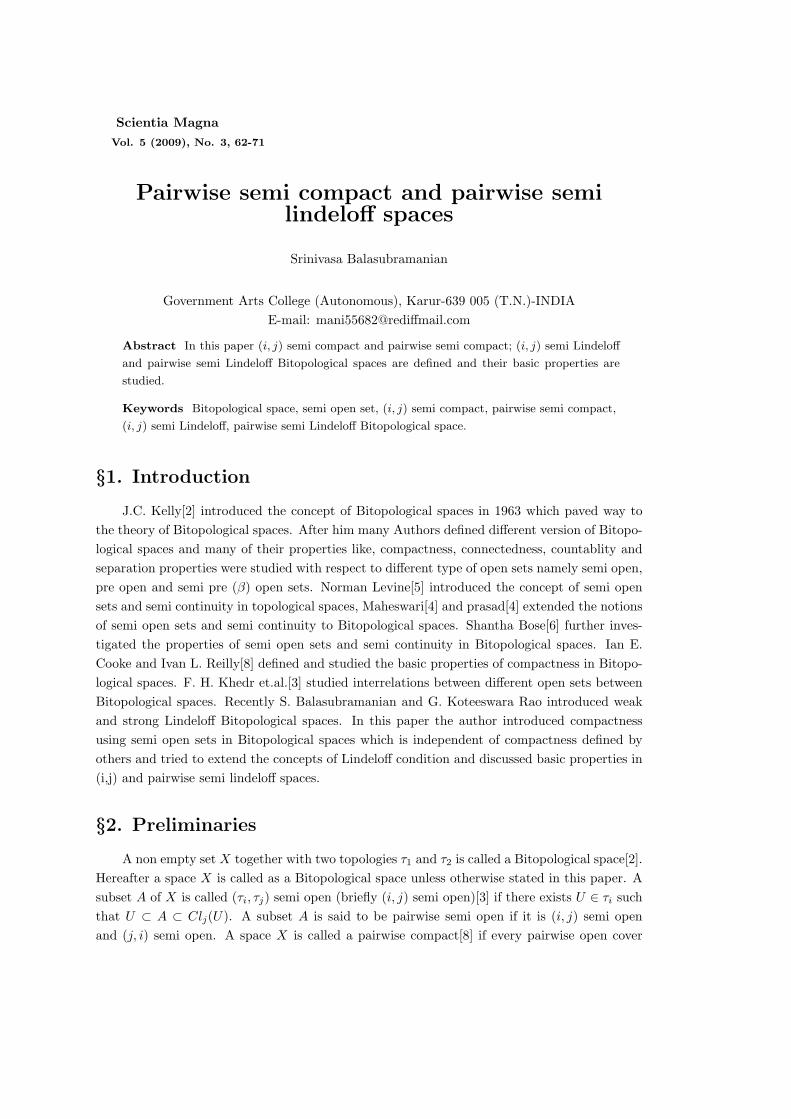
Scientia MagnaVol. 5 (2009), No. 3, 62-71
Pairwise semi compact and pairwise semilindeloff spaces
Srinivasa Balasubramanian
Government Arts College (Autonomous), Karur-639 005 (T.N.)-INDIAE-mail: [email protected]
Abstract In this paper (i, j) semi compact and pairwise semi compact; (i, j) semi Lindeloff
and pairwise semi Lindeloff Bitopological spaces are defined and their basic properties are
studied.
Keywords Bitopological space, semi open set, (i, j) semi compact, pairwise semi compact,
(i, j) semi Lindeloff, pairwise semi Lindeloff Bitopological space.
§1. Introduction
J.C. Kelly[2] introduced the concept of Bitopological spaces in 1963 which paved way tothe theory of Bitopological spaces. After him many Authors defined different version of Bitopo-logical spaces and many of their properties like, compactness, connectedness, countablity andseparation properties were studied with respect to different type of open sets namely semi open,pre open and semi pre (β) open sets. Norman Levine[5] introduced the concept of semi opensets and semi continuity in topological spaces, Maheswari[4] and prasad[4] extended the notionsof semi open sets and semi continuity to Bitopological spaces. Shantha Bose[6] further inves-tigated the properties of semi open sets and semi continuity in Bitopological spaces. Ian E.Cooke and Ivan L. Reilly[8] defined and studied the basic properties of compactness in Bitopo-logical spaces. F. H. Khedr et.al.[3] studied interrelations between different open sets betweenBitopological spaces. Recently S. Balasubramanian and G. Koteeswara Rao introduced weakand strong Lindeloff Bitopological spaces. In this paper the author introduced compactnessusing semi open sets in Bitopological spaces which is independent of compactness defined byothers and tried to extend the concepts of Lindeloff condition and discussed basic properties in(i,j) and pairwise semi lindeloff spaces.
§2. Preliminaries
A non empty set X together with two topologies τ1 and τ2 is called a Bitopological space[2].Hereafter a space X is called as a Bitopological space unless otherwise stated in this paper. Asubset A of X is called (τi, τj) semi open (briefly (i, j) semi open)[3] if there exists U ∈ τi suchthat U ⊂ A ⊂ Clj(U). A subset A is said to be pairwise semi open if it is (i, j) semi openand (j, i) semi open. A space X is called a pairwise compact[8] if every pairwise open cover

Vol. 5 Pairwise semi compact and pairwise semi lindeloff spaces 63
U ∈ τi ∪ τj has a finite sub cover. A space is called a weak (strong) [locally] compact if it iseither τi or τj(τi and τj) [locally] compact.
Definition 2.1.[6] A subset A of a topological space (X, τ) is said to be a semi open setif there is an open set U of X such that U ⊂ A ⊂ cl(U). A function f : (X, τ) → (Y, σ)[6] issaid to be semi continuous if for each V ∈ σ, f−1(V ) is semi open in X.
Definition 2.2.[3] A ⊆ (X, τi, τj) is said to be (i,j) semi open if there exists U ∈ τi suchthat U ⊂ A ⊂ clj(U).
Example 1. Let X be the real plane τi the half open rectangle topology and τj be theusual topology on X. A = (x, y)/0 ≤ x < 1, 0 ≤ y < 1 ∪ (1, 1) is τi semi open w.r.to τj butneither τi open nor τj open.
Example 2. Let X be the real line τi be the lower limit topology on X and τj the usualtopology on X. A = x/0 ≤ x < 1 is τi semi open w.r.to τj but neither τi open nor τj open.
Definition 2.3. Let f : (X, τi, τj) → (Y, σi, σj) be a function then f is said to be pairwisecontinuous[resp. pairwise open map] if the induced functions f : (X, τi) → (Y, σi) and f :(X, τj) → (Y, σj) are both continuous [resp. open].
Definition 2.4.[3] Let f : (X, τi, τj) → (Y, σi, σj) be a single valued function then f is saidto be pairwise semi continuous if the inverse image of each σi-open set of Y is (i, j) semi openin X, where i 6= j, i, j = 1, 2.
Theorem 2.5.[3] Let A be a subset of (X, τi, τj). If there exists an (i, j) semi open set U
such that U ⊂ A ⊂ clj(U), then A is (i, j) semi open.
Theorem 2.6.[3] The union of arbitrarily many (i, j) semi open sets is (i, j) semi open.
Proof. Let Ak/k ∈ K be a collection of (i, j) semi open sets in (X, τi, τj). For each k ∈K, ∃ aτi-open set Uk such that Uk ⊂ Ak ⊂ clj(Uk), then ∪Uk ⊂ ∪Ak ⊂ ∪clj(Uk) = clj(∪Uk).Put U = ∪Uk, U is τi-open. Thus ∪Ak is (i, j) semi open.
Theorem 2.7.[3] Let A ⊂ Y ⊂ X where X is a Bitopological space. If A is (i, j) semiopen in X, it is (i, j) semi open in Y .
Theorem 2.8.[3] Let f : (X, τi, τj) → (Y, σi, σj) be pairwise continuous pairwise openmap. If A is (i, j) semi open in X then f(A) is (i, j) semi open in Y .
Proof. Let A be(i, j) semi open in X, then there exists U ∈ τi such that U ⊂ A ⊂ clj(U).Now f(U) ⊂ f(A) ⊂ f(clj(U)), f(U) is σi-open, f being open map and f(clj(U)) ⊂ clj(f(U)), fbeing continuous. f(A) is (i, j) semi open in X.
Theorem 2.9.[3] Let f : (X, τi, τj) → (Y, σi, σj) be pairwise semi continuous pairwiseopen map. If A is (i, j) semi open in Y then f−1(A) is (i, j) semi open in X.
Proof. Let A be (i, j) semi open in Y , then there exists W ∈ σi such that W ⊂ V ⊂clj(W ). Since f is pairwise open, it follows that f−1(W ) ⊂ f−1(V ) ⊂ f−1(clj(W )) ⊂ clj(f−1(W )).Since f is pairwise semi continuous, f−1(W ) is (i, j) semi open in X. By theorem 2.5, f−1(V ) is(i, j) semi open in X.
Remark 1. [3] τi open ⇒ (i, j) semi open.

64 Srinivasa Balasubramanian No. 3
§3. (i, j) Semi compact Bitopological space
Definition 3.1. (X, τi, τj) is said to be (i) (i, j) semi compact if each (i, j) semi opencover has a finite (i,j) semi open sub cover. (ii) locally (i, j) semi compact if each x ∈ X has(i, j) semi-open neighborhood with compact (i, j) semi closure.
Example 3. since every open set is (i, j) semi open, example X = R, τi = Rι, τj = RΩ;where RΩ = minimum well ordered uncountable set will act as the example for these twodefinitions.
Example 4. Let X = [a, b] be the subspace of real numbers with τi = [a, c)/a < c < band τj = (c, d)/c < d as basic open sets then, (X, τi, τj) is (i, j) semi compact Bitopologicalspace.
Theorem 3.2. Every (i, j) semi compact space is locally (i, j) semi compact.
Theorem 3.3. Let (X, τi, τj) be Bitopological space and A ⊂ (X, τi, τj). Then A is (i, j)semi compact subset of (X, τi, τj) if the subspace (A, τi/A, τj/A) is (i, j) semi compact.
Theorem 3.4. A τi-closed subspace of a [locally] (i, j)semi compact space is [locally] (i, j)semi compact. The product of two [locally] (i, j) semi compact spaces is [locally] (i, j) semicompact.
Proof. A ⊆ (X, τi, τj) is τi-closed and (X, τi, τj) is (i, j) semi compact. For U = Ui/i ∈ Iis (i, j) semi open cover of A we can find U
′= G(U)/U ∈ U ∪ X − A an (i, j) semi open
cover of X, where G is such that U = G ∩ A, which implies U′
admits finite sub cover givingrise to the finite sub covers for U . Hence (A, τi/A, τj/A) is (i, j) semi compact.
A ⊆ (X, τi, τj) is τi-closed, (X, τi, τj) is locally (i, j) semi compact and x ∈ A ⊆ X beany point. Thenx has (i, j) semi compact neighborhood G. Since G is (i, j) semi compact, bytheorem 3.3 we can find (i, j) semi compact neighborhood U = G ∩A. Hence (A, τi/A, τj/A) islocally (i, j) semi compact.
Direct consequence of Tychnoff’s theorem.
Theorem 3.5. Let (X, τi, τj) be any [locally] (i, j) semi compact Bitopological space.Then (X, τi) is [locally] compact.
Proof. Let Gi/i ∈ I be any τi open cover for X. since every τi open set is (i, j) semiopen set, τi open cover will become (i, j) semi open cover and this contains finite (i, j) semi opencover. Since (X, τi, τj) is (i, j) semi compact. Therefore (X, τi) is compact. Similar argumentgives the proof of the second part.
Corollary 3.6. If (X, τi, τj) be any (i, j) semi compact Bitopological space. Then (X, τi)is locally compact.
Theorem 3.7. A Bitopological space is (i, j) semi compact iff (i) Every class of (i, j) semiclosed sets with empty intersection has a finite subclass with empty intersection. (ii) iff Everyclass of (i, j) semi closed sets with finite intersection property has non empty intersection. (iii)iff Every basic (i, j) semi open cover has a finite sub cover.
Corollary 3.8. A Bitopological space is (i, j) semi compact iff (i) Every class of τi-closedsets with empty intersection has a finite subclass with empty intersection. (ii) iff Every class ofτi-closed sets with finite intersection property has non empty intersection. (iii) iff Every τi-basicopen cover has a finite sub cover.

Vol. 5 Pairwise semi compact and pairwise semi lindeloff spaces 65
Theorem 3.9. Let f : (X, τi, τj) → (Y, σi, σj) be a pairwise semi continuous pairwise openmap and (X, τi, τj) is (i, j) semi compact. Then f(X) is (i, j) semi compact.
Proof. Let Gi/i ∈ I be (i, j) semi open cover for f (X). Since f is pairwise semi contin-uous, f−1(Gi)/i ∈ I is (i, j) semi open cover for X and has a finite (i, j) semi open sub cover.Therefore, for f is pairwise open, Gi/i ∈ I has a finite semi open sub cover. Thus f(X) is(i, j) semi compact.
Theorem 3.10. Let f : (X, τi, τj) → (Y, σi, σj) be a pairwise semi continuous pairwiseopen map and (Y, σi, σj) is (i, j) semi compact. Then f−1(Y ) is (i, j)semi compact.
Proof. Let Gi/i ∈ I be (i, j) semi open cover for f−1(Y ) implies each Gi is (i, j) semiopen set in f−1(Y ), then there exists U ∈ τi such that U ⊂ A ⊂ clj(U). Since f is pairwise semicontinuous, we have f(U) ⊂ f(A) ⊂ f(clj(U)) ⊂ clj(f(U)). This shows that f(Gi) is (i, j) semiopen in Y and hence f(Gi)/i ∈ I is (i, j) semi open cover for Y and has a finite (i, j) semiopen sub cover. Since (Y, σi, σj) is (i, j) semi compact. Therefore Gi/i ∈ I has a finite semiopen sub cover. Thus f−1(Y ) is (i, j) semi compact.
Corollary 3.11. Let f : (X, τi, τj) → (Y, σi, σj) be pairwise continuous pairwise open mapand (Y, σi, σj) is (i, j) semi compact. Then f−1(Y ) is (i, j) semi compact.
Proof. since every pairwise continuous map is pairwise semi continuous, result followsdirectly from the above theorem.
Remark 2. [locally] (i, j) semi compact is weak hereditary.
§4. Pairwise semi compact Bitopological space
Definition 4.1. (X, τi, τj) is said to be (i) pairwise semi compact if it is (i, j) and (j, i)semi compact. (ii) locally pairwise semi compact if it is locally (i, j) semi compact and locally(j, i) semi compact.
Example 5. Let R be the space of reals with topologies τi and τj , where τi has (a, b]as basic open sets, and τj has [a, b), a < b as basic open sets, then (X, τi, τj) pairwise semicompact.
Example 6. since every open set is (i, j) semi open, (X, τi, τj), where X = R, τi =Gn/Gn = (−n, n)n ∈ Z+; τj = RΩ will act as the example for these two definitions.
Theorem 4.2. Every pairwise semi compact space is locally pairwise semi compact.Proof. obvious from the definitions of pairwise semi compact and locally pairwise semi
compact spaces.Theorem 4.3. Let (X, τi, τj) be Bitopological space and A ⊆ (X, τi, τj). Then A is pair-
wise semi compact subset of (X, τi, τj) iff the subspace (A, τi/A, τj/A) is pairwise semi compactTheorem 4.4. A Bi-closed subspace of a [locally] pairwise semi compact space is [locally]
pairwise semi compact. The product of two [locally] pairwise semi compact spaces is [locally]pairwise semi compact.
Proof. A ⊆ (X, τi, τj) is Bi-closed and (X, τi, τj) is pairwise semi compact. Let U =Ui/i ∈ I, V = Vi/i ∈ I are respectively (i, j) and (j, i) semi open covers of A with respectto τi/A and τj/A then for each Ui ∈ U and for each Vi ∈ V , fix an (i, j) semi open set G andan (j, i) semi open set H such that U = G∩A, V = H ∩A, then the families U
′= G(U)/U ∈

66 Srinivasa Balasubramanian No. 3
U ∪ X − A and V′= H(V )/V ∈ V ∪ X − A are (i,j) and (j, i) semi open covers of X
with respect to τi and τj respectively, which implies U′and V
′admits finite sub covers which
in turn gives rise to the finite sub covers for U and V respectively. Hence (A, τi/A, τj/A) ispairwise semi compact
Direct from Tychnoff’s theorem.Theorem 4.5. Let (X, τi, τj) be any [locally] pairwise semi compact Bitopological space.
Then (X, τi) and (X, τj) are [locally] compact.Corollary 4.6. If (X, τi, τj) be any pairwise semi compact Bitopological space. Then
(X, τi) and (X, τj) are locally compact.Theorem 4.7. A Bitopological space is Pairwise semi compact iff (i) Every class of pairwise
closed sets with empty intersection has a finite subclass with empty intersection. (ii) iff Everyclass of pairwise closed sets with finite intersection property has non empty intersection. (iii)iff Every pairwise basic open cover has a finite sub cover.
Theorem 4.8. A Bitopological space is Pairwise semi compact iff (i) Every class of Bi-closed sets with empty intersection has a finite subclass with empty intersection. (ii) iff Everyclass of Bi-closed sets with finite intersection property has non empty intersection. (iii) iff Everypairwise basic open cover has a finite sub cover.
Theorem 4.9. Let f : (X, τi, τj) → (Y, σi, σj) be a pairwise semi continuous pairwise openmap and (X, τi, τj) is pairwise semi compact. Then f(X) is pairwise semi compact.
Proof. Let Gi/i ∈ I be pairwise semi open cover for f(X). Then Gi/i ∈ I is both(i, j) and (j, i) semi open covers for f(X). since f is pairwise semi continuous, f−1(Gi)/i ∈ Iis pairwise semi open cover for X and has a finite pairwise semi open sub cover. Therefore, forf is pairwise open, Gi/i ∈ I has a finite semi open sub cover. Thus f(X) is pairwise semicompact.
Theorem 4.10. Let f : (X, τi, τj) → (Y, σi, σj) be a pairwise semi continuous pairwiseopen map and (Y, σi, σj) is pairwise semi compact. Then f−1(Y ) is pairwise semi compact.
Proof. Let Gi/i ∈ I be pairwise semi open cover for f−1(Y ) implies f(Gi)/i ∈ I ispairwise semi open cover for Y and has a finite pairwise semi open sub cover. Since (Y, σi, σj)is pairwise semi compact. Therefore Gi/i ∈ I has a finite semi open sub cover. Thus f−1(Y )is pairwise semi compact.
Theorem 4.11. Let f : (X, τi, τj) → (Y, σi, σj) be pairwise continuous pairwise open mapand (Y, σi, σj) is pairwise semi compact. Then f−1(Y ) is pairwise semi compact.
Proof. since every pairwise continuous map is pairwise semi continuous, result followsdirectly from the above theorem.
Example 7. X = R; τi = φ,R, (a,∞) : a ∈ R; τj = φ,R, (−∞, a) : a ∈ R then(X, τi, τj) is not (i,j) and pairwise semi compact. But according to Cooke and Reilly it ispairwise compact.
Example 8. X = [0, 1]; τi = φ, X, 0, [0, a) : a ∈ X; τj = φ, X, 1, (a, 1] : a ∈ Xthen (X, τi, τj) is pairwise semi compact. According to Cooke and Reilly it is pairwise B-compact.
Example 9. X = a, b, c; τi = φ, X, a, b, c; τj = φ, X, a, b, c then(X, τi, τj) is not B-compact according to Cooke and Reilly. Since a, b, c is a τj open

Vol. 5 Pairwise semi compact and pairwise semi lindeloff spaces 67
cover of X without τi open sub cover.Example 10. X = R2; τi = usual topology; τj = Half open rectangle topology; A =
(x, y)/0 ≤ x < 1; 0 ≤ y < 1 ∪ (1, 1) is τj semi open w.r.to τi but neither τi open nor τj open.Remark 3. [locally] pairwise semi compact is weak hereditary.
§5. (i, j) Semi second countability
Definition 5.1.(i) (X, τi, τj) is said to be (i, j) semi second countable if it has countable (i, j) semi open base.(ii) (X, τi, τj) is said to be (i, j) semi first countable if each x in X has countable (i, j) semiopen base.
Example 11. (X, τi, τj) is (i, j) semi second countable, where X = R, τi = Rι; τj =Gn/Gn = (−n, n) : n ∈ N.
Theorem 5.2.(i) Any subspace of (i, j) semi [first] second countable space is (i, j) semi [first] second countable.(ii) Any countable product of (i, j) semi [first] second countable spaces is (i, j) semi [first] secondcountable.
Proof. (i) Let (A, τi/A, τj/A) be any subspace of an (i, j) semi second countable space(X, τi, τj) and since (X, τi, τj) is (i, j) semi second countable, there exists countable (i, j) semi-open base Gi, which in turn gives Hi = Gi ∩ A a countable (i/A, j/A) semi open base for(A, τi/A, τj/A). Hence (A, τi/A, τj/A) is (i, j) semi second countable. Similar argument shows(A, τi/A, τj/A) is (i, j) semi first countable.
(ii) Let X = ΠXi; X′is are (i, j) semi second countable spaces and Bi = Bj
i /j ∈ Jis countable (i, j) semi open base for each Xi with respect to τ i
1 and τ i2 respectively. Then
B = ΠBi = Ui/Ui = ΠBji where Bj
i ∈ Bi for finite i and Bj = Xj for j 6= i, is the countable(i, j) semi open base in (X, τ1, τ2) where τ1 = Πi∈Iτ
i1, τ2 = Πi∈Iτ
i2. Hence X = ΠXi is (i, j)
semi second countable. Similar argument shows X = ΠXi is (i, j) semi first countable.Corollary 5.3. Let (X, τi, τj) be any (i, j) semi [first] second countable Bitopological
space. (i) Any subspace of (X, τi) [first] second countable space is (i, j) semi [first] secondcountable. (ii) Any countable product of (X, τi) [first] second countable spaces is (i, j) semi[first] second countable.
Remark 4. The property of (i, j) semi [first] second countability is hereditary.
§6. Pairwise semi second countability
Definition 6.1. (X, τi, τj) is said to be pairwise semi second [first] countable if it is both(i, j) and (j, i) semi second [first] countable.
Example 12. X = countable set; τi = cofinite topology and τj = discrete topology, ispairwise semi second countable.
Theorem 6.2. (i) Any subspace of pairwise semi [first] second countable space is pairwisesemi [first] second countable. (ii) Any countable product of pairwise semi [first] second countablespaces is pairwise semi [first] second countable.

68 Srinivasa Balasubramanian No. 3
Proof. (i) Let (A, τi/A, τj/A) be any subspace of pairwise semi second countable space(X, τi, τj). B = Bi/i ∈ I, B
′= B′
i/i ∈ I are respectively countable (i, j) and (j, i) semiopen bases in X. Then C = Ci/Ci = Bi ∩ Ai∈I , C
′= C ′
i/C′i = B
′i ∩ Ai∈I are countable
(i/A, j/A) and (j/A, i/A) semi open bases for A. Therefore (A, τi/A, τj/A) is pairwise semi secondcountable. Similar argument shows (A, τi/A, τj/A) is pairwise semi first countable.
(ii) Let X = ΠXi; X′is are pairwise semi second countable, Bi = Bj
i /j ∈ J and B′i =
B′ij/j ∈ J are countable (i, j) and (j, i) semi open bases for each Xi with respect to τ i
1 and τ i2
respectively. Then B = ΠBi = Ui/Ui = ΠBij where Bji ∈ Bi for finite i, and Bj = Xj for j 6=
i, B′= ΠB
′i = U ′
i /U′i = ΠB
′ij where B
′ij ∈ B
′i for finite i, and B
′j = Xj for j 6= i are
respectively the countable(i, j) and (j, i) semi open bases in (X, τ1, τ2) where τ1 = Πi∈Iτi1, τ2 =
Πi∈Iτi2. Hence X = ΠXi is pairwise semi second countable. Similar argument shows X = ΠXi
is pairwise semi first countable.Proofs of the following are trivial and so left to the reader.Definition 6.3. (X, τi, τj) is said to be Bi second countable if it is both τi and τj second
countable.Corollary 6.4. Let (X, τi, τj) be any Bitopological space. (i) Every Bi [first] second
countable Bitopological space is pairwise semi [first] second countable.Corollary 6.5. Let (X, τi, τj) be any Bitopological space. (i) Any subspace of Bi first
[second] countable space is pairwise semi first [second] countable. (ii) Any countable productof Bi first [second] countable space is pairwise semi first [second] countable.
Remark 5. The property of pairwise semi [first] second countability is hereditary.
§7. (i, j) semi Lindeloff Bitopological space
Definition 7.1. (X, τi, τj) is said to be (i, j) semi Lindeloff if each (i, j)semi open coverhas a countable (i, j) semi open sub cover and (X, τi, τj) is locally (i, j) semi Lindeloff if eachx ∈ X has (i, j) semi Lindeloff neighborhood.
Example 13. Let X be the real line τi the lower limit topology and τj be the upper limittopology on X, then (X, τi, τj) is (i, j) semi Lindeloff.
Theorem 7.2. Suppose (X, τi, τj) has a countable (i, j) semi open base then every semiopen cover of (X, τi, τj) contains a countable sub collection covering (X, τi, τj).
Proof. Let B = Bn/n ∈ N is (i, j) countable semi open base for X. Let U = Ui/i ∈ Ibe (i, j) semi open covering of X. For each n ∈ N , choose an element Un of U such that Bn ⊆ Un.Then the collection U
′= Un/n ∈ N is countable. Furthermore, it covers X. Given a point
x ∈ X, we can choose an element Un of U containing x. Since Un is (i, j) semi open, thereexists basis elements Bn, such that x ∈ Bn ⊆ A. Since Bn ⊆ Un, it contains x. Thereforex ∈ Bn ⊆ Un. Thus U
′is a countable sub collection of U which covers X with respect to τi
and τj respectively. Hence the theorem.Theorem 7.3. (i) A τi-closed subspace of a [locally] (i, j) semi Lindeloff space is [locally]
(i, j) semi Lindeloff. (ii) The product of two [locally] (i, j) semi Lindeloff spaces need not be[locally] (i, j) semi Lindeloff.
Proof. (i) Let A be τi-closed subspace of (i, j) semi Lindeloff space (X, τi, τj). Let U =
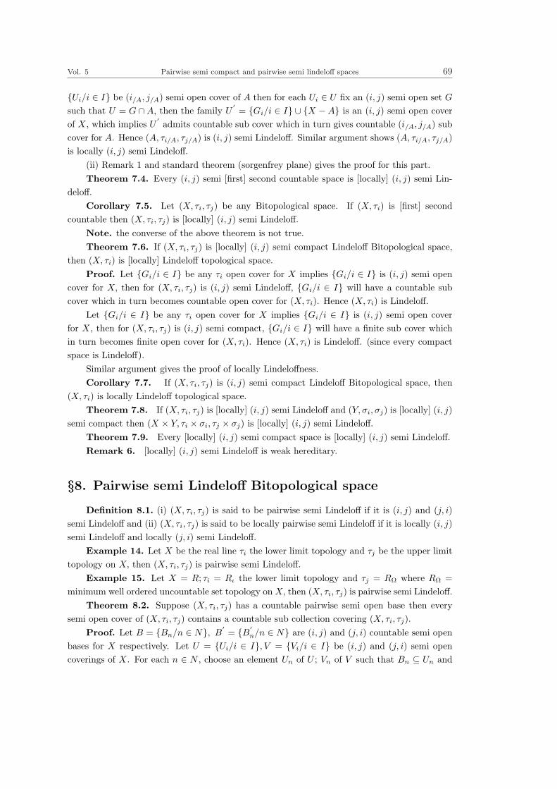
Vol. 5 Pairwise semi compact and pairwise semi lindeloff spaces 69
Ui/i ∈ I be (i/A, j/A) semi open cover of A then for each Ui ∈ U fix an (i, j) semi open set G
such that U = G ∩ A, then the family U′= Gi/i ∈ I ∪ X − A is an (i, j) semi open cover
of X, which implies U′admits countable sub cover which in turn gives countable (i/A, j/A) sub
cover for A. Hence (A, τi/A, τj/A) is (i, j) semi Lindeloff. Similar argument shows (A, τi/A, τj/A)is locally (i, j) semi Lindeloff.
(ii) Remark 1 and standard theorem (sorgenfrey plane) gives the proof for this part.Theorem 7.4. Every (i, j) semi [first] second countable space is [locally] (i, j) semi Lin-
deloff.Corollary 7.5. Let (X, τi, τj) be any Bitopological space. If (X, τi) is [first] second
countable then (X, τi, τj) is [locally] (i, j) semi Lindeloff.Note. the converse of the above theorem is not true.Theorem 7.6. If (X, τi, τj) is [locally] (i, j) semi compact Lindeloff Bitopological space,
then (X, τi) is [locally] Lindeloff topological space.Proof. Let Gi/i ∈ I be any τi open cover for X implies Gi/i ∈ I is (i, j) semi open
cover for X, then for (X, τi, τj) is (i, j) semi Lindeloff, Gi/i ∈ I will have a countable subcover which in turn becomes countable open cover for (X, τi). Hence (X, τi) is Lindeloff.
Let Gi/i ∈ I be any τi open cover for X implies Gi/i ∈ I is (i, j) semi open coverfor X, then for (X, τi, τj) is (i, j) semi compact, Gi/i ∈ I will have a finite sub cover whichin turn becomes finite open cover for (X, τi). Hence (X, τi) is Lindeloff. (since every compactspace is Lindeloff).
Similar argument gives the proof of locally Lindeloffness.Corollary 7.7. If (X, τi, τj) is (i, j) semi compact Lindeloff Bitopological space, then
(X, τi) is locally Lindeloff topological space.Theorem 7.8. If (X, τi, τj) is [locally] (i, j) semi Lindeloff and (Y, σi, σj) is [locally] (i, j)
semi compact then (X × Y, τi × σi, τj × σj) is [locally] (i, j) semi Lindeloff.Theorem 7.9. Every [locally] (i, j) semi compact space is [locally] (i, j) semi Lindeloff.Remark 6. [locally] (i, j) semi Lindeloff is weak hereditary.
§8. Pairwise semi Lindeloff Bitopological space
Definition 8.1. (i) (X, τi, τj) is said to be pairwise semi Lindeloff if it is (i, j) and (j, i)semi Lindeloff and (ii) (X, τi, τj) is said to be locally pairwise semi Lindeloff if it is locally (i, j)semi Lindeloff and locally (j, i) semi Lindeloff.
Example 14. Let X be the real line τi the lower limit topology and τj be the upper limittopology on X, then (X, τi, τj) is pairwise semi Lindeloff.
Example 15. Let X = R; τi = Rι the lower limit topology and τj = RΩ where RΩ =minimum well ordered uncountable set topology on X, then (X, τi, τj) is pairwise semi Lindeloff.
Theorem 8.2. Suppose (X, τi, τj) has a countable pairwise semi open base then everysemi open cover of (X, τi, τj) contains a countable sub collection covering (X, τi, τj).
Proof. Let B = Bn/n ∈ N, B′= B′
n/n ∈ N are (i, j) and (j, i) countable semi openbases for X respectively. Let U = Ui/i ∈ I, V = Vi/i ∈ I be (i, j) and (j, i) semi opencoverings of X. For each n ∈ N , choose an element Un of U ; Vn of V such that Bn ⊆ Un and

70 Srinivasa Balasubramanian No. 3
B′n ⊆ Vn respectively. Then the collection U
′= Un/n ∈ N; V
′= Vn/n ∈ N are countable.
Furthermore, they covers X with respect to (i, j) and (j, i) respectively. Given a point x ∈ X,we can choose an element Un of U containing x and Vn of V containing x. Since Un, Vn are(i, j) and (j, i) semi open respectively, there exists basis elements Bn, B
′n such that x ∈ Bn ⊆ A
and x ∈ B′n ⊆ A. Since Bn ⊆ Un, B
′n ⊆ Vn they both contains x. Therefore x ∈ Bn ⊆ Un and
x ∈ B′n ⊆ Vn. Thus U
′is a countable sub collection of U ; V
′is a countable sub collection of
V , which covers X with respect to τ1 and τ2 respectively. Hence the theorem.
Definition 8.3. A subset in (X, τi, τj) is said to be a Bi-closed set if it is both τi and τj
closed.
Theorem 8.4. (i) A Bi-closed subspace of a [locally] pairwise semi Lindeloff space is[locally] pairwise semi Lindeloff. (ii) The product of two [locally] pairwise semi Lindeloff spacesneed not be [locally] pairwise semi Lindeloff.
Proof. (i) Let A be Bi-closed subspace of pairwise semi Lindeloff space (X, τi, τj). LetU = Ui/i ∈ I, V = Vi/i ∈ I are respectively (i/A, j/A) and (j/A, i/A) semi open coversof A then for each Ui ∈ U and for each Vi ∈ V , fix an (i, j) semi open set G and (j,i) semiopen set H such that U = G ∩ A, V = H ∩ A, then the families U
′= Gi/i ∈ I ∪ X − A
and V′= Hi/i ∈ I ∪ X − A are (i, j) and (j, i) semi open covers of X respectively, which
implies U′
and V′
admits countable sub covers which in turn gives countable sub covers forA. Hence (A, τi/A, τj/A) is pairwise semi Lindeloff. Similar argument shows (A, τi/A, τj/A) islocally pairwise semi Lindeloff.
(ii) Let (X, τi, τj) be pairwise semi Lindeloff space, where X = R, τi = Rι, τj = Rυ thenX × X is the product of two pairwise semi Lindeloff spaces called sorgenfrey planes. It hasbasis all sets of the form [a, b)X[c, d) and (b,−a]X(d, c] in the planes. Consider the subspacesL = xX(−x)/x ∈ Rι and L
′= (−x)Xx/x ∈ Rυ in R2
ι and R2υ respectively. Then obviously
L and L′are (i, j) and (j, i) semi closed in R2
ι and R2υ respectively. By covering R2 by the (i, j)
semi open sets R2ι − L and by the basis elements of the form [a, b)X[−a, d) and by (j, i) semi
open sets R2υ − L
′and by the basis elements of the form (b,−a]X[d, a) we can see that each of
these basis elements in R2ι and R2
υ intersects L and L′in at most one point respectively. Since
both L and L′are uncountable, no countable sub collection covers R2
ι and R2υ respectively. Thus
the product of two pairwise semi Lindeloff Bitopological spaces is not pairwise semi Lindeloff.
Theorem 8.5. Every Bi - [first] second countable space is [locally] pairwise semi Lindeloff.
Theorem 8.6. If (X, τi, τj) is [locally] pairwise semi compact Lindeloff Bitopologicalspace, then (X, τi) and (X, τj) are [locally] Lindeloff topological spaces
Proof. Let Gi/i ∈ I be any τi open cover for X implies Gi/i ∈ I is (i, j) semi opencover for X, then for (X, τi, τj) is (i, j) semi Lindeloff, Gi/i ∈ I will have a countable subcover which in turn becomes countable open cover for (X, τi). Hence (X, τi) is Lindeloff.
Let Gi/i ∈ I be any τi open cover for X implies Gi/i ∈ I is (i, j) semi open cover forX, then for (X, τi, τj) is (i, j) semi compact, Gi/i ∈ I will have a finite sub cover which inturn becomes finite open cover for (X, τi). Hence (X, τi) is Lindeloff(since every compact spaceis Lindeloff).
Similar argument gives the proof of locally Lindeloffness.
Corollary 8.7. If (X, τi, τj) is pairwise semi (compact)Lindeloff Bitopological space, then

Vol. 5 Pairwise semi compact and pairwise semi lindeloff spaces 71
(X, τi) and (X, τj) are locally Lindeloff topological space.Theorem 8.8. If (X, τi, τj) is [locally] pairwise semi Lindeloff and (Y, σi, σj) is [locally]
pairwise semi compact then (X × Y, τi × σi, τj × σj) is [locally] pairwise semi Lindeloff.Corollary 8.9. If (X, τi, τj) is pairwise semi Lindeloff and (Y, σi, σj) is pairwise semi
compact then (X × Y, τi × σi, τj × σj) is pairwise locally semi Lindeloff.Theorem 8.10. Every [locally] pairwise semi compact space is [locally] pairwise semi
Lindeloff.Proof. Let (X, τi, τj) is pairwise semi compact. Then for Gi an (i, j) and G
′i an (j, i) semi
open covers with finite (i, j) and (j, i) semi open covers for X respectively. Since every finitecover is countable cover, Gi an (i, j) and G
′i an (j, i) are semi open covers with countable (i, j)
and (j, i) semi open sub covers for X respectively. Hence (X, τi, τj) is pairwise semi Lindeloff.Trivial verification shows (X, τi, τj) is [locally] pairwise semi Lindeloff.
Remark 7. [locally] pairwise semi Lindeloff is weak hereditary.Conclusion. In this paper we defined new compactness and Lindeloffness in Bitopological
spaces and studied their interrelations.Acknowledgement. The Author would like to thank referees for their valuable comments
and suggestions.
References
[1] U. N. B. Dissanayake and K.P.R. Sastry, Locally Lindeloff spaces-Indian Journal ofPure and Applied Mathematics, 18(1987), No. 10, 876-881.
[2] J. C. Kelly, Bitopological spaces-Proc. London Math. Soc., 13(1963), No. 3, 71-89.[3] F. H. Khedr, S. M. Al-Areefi, pre continuity and semi-pre continuity in Bitopological
spaces-Indian Journal of Pure and Applied Mathematics, 23(1992), No. 9, 625-633.[4] S. N. Maheswari and R. Prasad, semi open sets and semi continuity in Bitopological
spaces-Math. Notae, 26(1977/78), 29-37.[5] Norman Levine-semi open sets and semi continuity in topological spaces, Amer. Math.
Monthly, 70, 36.[6] Shantha Bose-semi open sets and semi continuity in Bitopological spaces, Bull cal.
Math. Soc., 73(1981), 237-246.[7] G. F. Simmons-Introduction to Topology and Modern Analysis, Tata McGraw Hill.[8] Ian E. Cooke and Ivan L. Reilly-On Bitopological Compactness Jr. London Math. Soc.,
9(1975), No. 2, 518-522.

Scientia MagnaVol. 5 (2009), No. 3, 72-75
A note on f-minimum functions
Jozsef Sandor
Babes-Bolyai University of Cluj, RomaniaE-mail: [email protected] [email protected]
Abstract For a given arithmetical function f : N → N, let F : N → N be defined by
F (n) = minm ≥ 1 : n|f(m), if this exists. Such functions, introduced in [4], will be called
as the f -minimum functions. If f satisfies the property a ≤ b =⇒ f(a)|f(b), we shall prove
that F (ab) = maxF (a), F (b) for (a, b) = 1. For a more restrictive class of functions, we
will determine F (n) where n is an even perfect number. These results are generalizations of
theorems from [10], [1], [3], [6].
Keywords Divisibility of integers, prime factorization, arithmetical functions, perfect numb-
ers.
§1. Introduction
Let N = 1, 2, . . . be the set of positive integers, and f : N → N a given arithmeticalfunction, such that for each n ∈ N there exists at least an m ∈ N such that n|f(m). In 1999and 2000 [4], [5], as a common generalization of many arithmetical functions, we have definedthe application F : N→ N given by
F (n) = minm ≥ 1 : n|f(m), (1)
called as the ”f -minimum function”. Particularly, for f(m) = m! one obtains the Smarandachefunction (see [10], [1])
S(n) = minm ≥ 1 : n|m!. (2)
Moree and Roskam [2], and independently the author [4], [5], have considered the Eulerminimum function
E(n) = minm ≥ 1 : n|ϕ(n), (3)
where ϕ is Euler’s totient. Many other particular cases of (1), as well as, their ”dual” oranalogues functions have been studied in the literature; for a survey of concepts and results,see [9].
In 1980 Smarandache discovered the following basic property of S(n) given by (2):
S(ab) = maxS(a), S(b) for (a, b) = 1. (4)
Our aim in what follows is to extend property (4) to a general class of f -minimum functions.Further, for a subclass we will be able to determine F (n) for even perfect numbers n.

Vol. 5 A note on f -minimum functions 73
§2. Main results
Theorem 1. Suppose that F of (1) is well defined. Then for distinct primes pi, andarbitrary αi ≥ 1 (i = 1, 2 · · · , r) one has
F
(r∏
i=1
pαii
)≥ maxF (pαi
i ) : i = 1, 2 · · · , r. (5)
The second result offers a reverse inequality:Theorem 2. With the notations of Theorem 1 suppose that f satisfies the following
divisibility condition:a|b =⇒ f(a)|f(b) (a, b ≥ 1) (∗)
Then one has
F
(r∏
i=1
pαii
)≤ l.c.m.F (pαi
i ) : i = 1, 2 · · · , r, (6)
where l.c.m. denotes the least common multiple.By replacing (∗) with another condition, a more precise result is obtainable:Theorem 3. Suppose that f satisfies the condition:
a ≤ b =⇒ f(a)|f(b) (a, b ≥ 1). (∗∗)
ThenF (mn) = maxF (m), F (n) for (m,n) = 1. (7)
Finally, we shall prove the following:Theorem 4. Suppose that f satisfies (∗∗) and the following two assumptions:(i) n|f(n); (ii) For each prime p and m < p we have p - f(n). (8)Let k be an even perfect number. Then
F (k) = k/2s, where 2s‖k. (9)
Remarks . (1) The function ϕ satisfies property (∗). Then relation (6) gives a result forthe Euler minimum function E(n) (see [7], [8]).
(2) Let f(m) = m!. Then clearly (∗∗) holds true. Thus (7) extends relation (4). Foranother example, let f(m) = l.c.m.1, 2, . . . , m. Then the function F given by (1) satisfiesagain (7), proved e.g. in [1].
(3) If f(n) = n!, then both (i) and (ii) of (8) are satisfied. This relation (9) for F ≡ S
follows. This was first proved in [3] (see also [6]).
§3. Proof of theorems
Theorem 1. There is no loss of generality to prove (5) for r = 2. Let pα, qβ be twodistinct prime powers. Then
F (pαqβ) = minn ≥ 1 : pαqβ |f(m) = m0,

74 Jozsef Sandor No. 3
so pαqβ |f(m0). This is equivalent to pα|f(m0), qβ |f(m0). By definition (1) we get m0 ≥ F (pα)and m0 ≥ F (qβ), i.e. F (pαqβ) ≥ maxF (pα), F (qβ). It is immediate that the same proofapplies to F
(∏pα
)≥ maxF (pα), where pα are distinct prime powers.
Theorem 2. Let F (pα) = m1, F (qβ) = m2. By definition (1) of function F it followsthat pα|F (m1) and qβ |F (m2). Let l.c.m.m1,m2 = g. Since m1|g, one has f(m1)|f(g) by (∗).Similarly, since m2|g, one can write f(m2)|f(g). These imply pα|f(m1)|f(g) and qβ |f(m2)|f(g),yielding pαqβ |f(g). By definition (1) this gives g ≥ F (pαqβ), i.e. l.c.m.F (pα), F (qβ) ≥F (pαqβ), proving the theorem for r = 2. The general case follows exactly by the same lines.
Theorem 3. By taking into account of (5), one needs only to show that the reverseinequality is true. For simplicity, let us consider again r = 2. Let F (pα) = m, F (qβ) = n
with m ≤ n. By definition (1) one has pα|f(m), qβ |f(n). Now, by assumption (∗∗) we canwrite f(m)|f(n), so pα|f(m)|f(n). Therefore, one has pα|f(n), qβ |f(n). This in turn impliespαqβ |f(n), so n ≥ F (pαqβ); i.e. maxF (pα), F (qβ) ≥ F (pαqβ). The general case followsexactly the same lines. Thus, we have proved essentially, that F (pαqβ) = maxF (pα), F (qβ),or more generally
F
(r∏
i=1
pαii
)= maxF (pαi
i ) : i = 1, 2 · · · , r. (10)
Now, relation (7) is an immediate consequence of (10), for by writing
m =r∏
i=1
pαii , n =
s∏
j=1
qβj
j , with (pi, qj) = 1,
it follows that
F (mn) = maxF (pαii ), F (qβj
j ) : i = 1, 2 · · · , r, j = 1, 2 · · · , s
= maxmaxE(pαii ) : i = 1, 2 · · · , r,maxE(qβj
j ) : j = 1, 2 · · · , s= maxF (m), F (n),
by equality (10).Theorem 4. By (i) and definition (1) we get
F (n) ≤ n. (11)
Now, by (i), one has p|f(p) for any prime p, but by (ii), p is the least such number. Thisimplies that
F (p) = p for any prime p. (12)
Now, let k be an even perfect number. By the Euclid-Euler theorem (see e.g. [7]) k maybe written as k = 2n−1(2n − 1), where p = 2n − 1 is a prime (”Mersenne prime”). Since (∗∗)holds true, by Theorem 3 we can write
F (k) = F (2n−1(2n − 1)) = maxF (2n−1), F (2n − 1).
Since F (2n − 1) = 2n − 1 (by (12)), and F (2n−1) ≤ 2n−1 (by (11)), from 2n−1 < 2n − 1
for n ≥ 2, we get F (k) = 2n − 1 =k
2s, where s = n − 1 and 2s‖k. This finishes the proof of
Theorem 4.

Vol. 5 A note on f -minimum functions 75
References
[1] C. Dumitrescu and V. Seleacu, The Smarandache function, Erhus Univ. Press, USA,1996.
[2] P. Moree and H. Roskam, On an arithmetical function related to Euler’s totient andthe discriminator, Fib. Quart., 33(1995), 332-340.
[3] S. M. Ruiz, Smarandache’s function applied to perfect numbers, Smarandache NotionsJ., 10(1999), No. 1-2-3, 114-115.
[4] J. Sandor, On certain generalizations of the Smarandache function, Notes NumberTheory Discr. Math., 5(1999), No. 2, 41-51.
[5] J. Sandor, On certain generalizations of the Smarandache function, Smarandache No-tions Journal, 11(2000), No. 1 -3, 202-212.
[6] J. Sandor, A note on S(n), where n is an even perfect number, Smarandache NotionsJ., 11(2000), No. 1-3, 139.
[7] J. Sandor and B. Crstici, Handbook of number theory II, Springer Verlag, 2005.[8] J. Sandor, On the Euler minimum and maximum functions, RGMIA, Research Report
Collection (Australia), 8(2005), No. 1, 125-130.[9] J. Sandor, On certain special functions of Number theory and Mathematical analysis,
to appear in Monograph on special functions (USA), 2007.[10] F. Smarandache, A function in the number theory, An. Univ. Timisoara, Ser. Mat.,
38(1980), 79-88.

Scientia MagnaVol. 5 (2009), No. 3, 76-86
Some Smarandache conclusions of coloringproperties of complete uniform mixed
hypergraphs deleted some C-hyperedges
Guobiao Zheng
Qinghai Institute for Nationalities Journal editorial board, Qinghai Xining, 810007
Abstract The upper and lower chromatic number of uniform mixed hypergraphs and C-hyperedge and D-hyperedge contact with the inevitable. In general, the increase in the C-hyperedge will increase lower chromatic number χH, an increase D-hyperedge will decrease
upper chromatic number χH. In this paper the relationship between C-hyperedge with the
upper chromatic number and lower chromatic number and some conclusions with respect to
mixed hypergraph are given.
Keywords A complete uniform mixed hypergraph, chromatic, upper chromatic, Smarand-
ache conclusions.
§1. Lemma and the basic concepts
Definition 1.1.[1] Let X = x1, x2, · · · , xn be a finite set, C = C1, C2, · · · , Cl, D =D1, D2, · · · , Dm are two subset clusters of X, all of which Ci ∈ C to meet |Ci| ≥ 2, and allDj ∈ D to meet |Dj | ≥ 2. Then H = (X, C,D) is called a mixed hypergraph from X, and eachCi ∈ C is called the C−hyperedges, and each Dj ∈ D is called the D−hyperedges. In particular,HD = (X,D) is called a D hypergraph, the HC = (X, C) for C− hypergraph.
Definition 1.2.[2] On 2 ≤ l, m ≤ n = |X|, let
K(n, l,m) = (X, C,D) = (X,
(X
l
),
(X
m
))
where |C| =(nl
)and |D| =
(nm
), then K(n, l,m) is called the complete (l, m)-uniform mixed
hypergraph with n vertex.It is clear that for a given n, l,m, in a sense of the isomorphic existence just has one
K(n, l, m).Definition 1.3.[3,4] For mixed hypergraphH = (X, C,D), the largest i among all existence
of strict i-Coloring known as the upper chromatic number H, said that for χH.Definition 1.4.[5] For mixed hypergraphH = (X, C,D), if a i Partition X = X1, X2, · · · ,
Xi of vertex sets X satisfy:1) For each C-hyperedge at least two vertices is allocated in the same block;2) For each D-hyperedge at least two vertices is allocated in different blocks.
The partition is called as a feasible partition of H.Obviously, any strict i coloring of H corresponds with a strict i feasible partition, and vice
versa. they are equivalent. Therefore, we write one feasible partition of H or a strict i-coloringc as: c = X1
⋃X2
⋃ · · ·⋃ Xi and ri(H) = ri is the total number of all feasible i partition.

Vol. 5Some Smarandache conclusions of coloring properties of complete uniform mixed
hypergraphs deleted some C-hyperedges 77
Definition 1.5.[6] Let S be a subset of the vertices set X of mixed hypergraph H =(X, C,D), if the set does not contain any of the C-Hyperedge (D-Hyperedge) as a subset, thenit is called C stable or C independent (D stable or D independent).
Lemma 1.1.[7,8] Let mixed hypergraph H = (X,(Xr
),D), where 2 ≤ r ≤ n = n(H), then
Arbitrary a coloring of H meet condition
χ(H) = r − 1.
Definition 1.6.[9] mixed hypergraph for H = (X, C,D), if there is a mapping c : Y →1, 2, · · · , λ that between subset Y ∈ X and λ colors 1, 2, · · · , λ, and it meet followingconditions:
1)For each C-hyperedge C ∈ C, at least two vertices are the same color;
2) For each D-hyperedge D ∈ D, at least two vertices are different colors.
Then, mapping c is called as one λ colors normal coloring of the mixed hypergraph H.
Definition 1.7.[10] In a normal i−coloring of H, if i colors are used, then the coloring iscalled a strict i-coloring.
It is clear that a normal χ(H)−coloring of mixed hypergraph H must be a strict coloring.
Definition 1.8.[11] For any coloring c of the mixed hypergraph H = (X, C,D), Let Y bea subset of X, then if Y satisfied: the arbitrary y1 ∈ Y, y2 ∈ Y , there is c(y1) = c(y2), then wecall the subset Y as monochrome; if each of two is different colors, that is, c(y1) 6= c(y2), thenwe call subset Y as the multi-color.
By the definitionthe of the normal coloring of mixed hypergraph, we know that for anynormal coloring of the hypergraph, D-hyperedge not is a subset of monochrome, C-hyperedgenot is a subset of the multi-color.
Definition 1.9.[12] In an arbitrary strictly i-coloring ofH, the vertex‘s set X ofH certainlyis divided into i partition, each partition is a non-empty subset of monochrome, we call it asthe color category.
Lemma 1.2.[13] Let mixed hypergraph H = (X, C,D), and n = |X|, then regardless Hcan normal coloring or not can, but the coloring of its sub-hypergraph HC and HD is alwaysavailable and there is χ(HC) = 1, r1(HC) = 1 and χ(HD) = n(H), rn(HD) = 1.
Lemma 1.3.[14] For mixed hypergraph H′ = (X, C, (Xm
)), if ∀C ∈ C , where |C| = k and
n(H′) ≤ (k − 1)(m− 1), then χ(H′) ≥ k − 1.
Lemma 1.4. Mixed hypergraph for H = (X, C,D), let H′be arbitrary a subhypergraph
of H, the χ(H) ≥ χ(H′), χ(H) ≤ χ(H′
).
Lemma 1.5.[15] For a colorable mixed hypergraphH = (X,(Xl
),(Xm
)), where 2 ≤ l, m ≤ n,
then
1) χ(H) = dn(H)m−1 e, χ(H) = l − 1;
2) H is the uncolorable if and only if dn(H)m−1 e ≥ l.
Lemma 1.6.[16] For C hypergraph H = (X, C, ∅), if ∀C ∈ C there are |C| ≥ k, thenχ(H) ≥ k − 1, and all (k − 1)-coloring of H are normal.
Lemma 1.7.[17] If m articles put into n box, then at least one box contain not less than⌈mn
⌉articles, where
⌈mn
⌉is not less than m
n smallest integer.
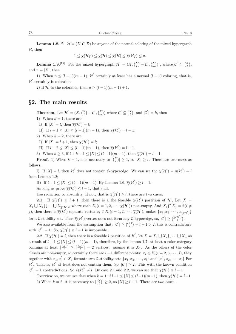
78 Guobiao Zheng No. 3
Lemma 1.8.[18] H = (X, C,D) be anyone of the normal coloring of the mixed hypergraphH, then
1 ≤ χ(HD) ≤ χ(H) ≤ χ(H) ≤ χ(HC) ≤ n.
Lemma 1.9.[19] For the mixed hypergraph H′= (X,
(Xl
) − C′ , (Xm
)) , where C′ ⊆ (
Xl
),
and n = |X|, then1) When n ≤ (l − 1)(m − 1), H′
certainly at least has a normal (l − 1) coloring, that is,H′
certainly is colorable.2) If H′
is the colorable, then n ≥ (l − 1)(m− 1) + 1.
§2. The main results
Theorem. Let H′= (X,
(Xl
)− C′ , (Xm
)) where C′ ⊆ (
Xl
), and |C′ | = k, then
1) When k = 1, there areI) If |X| = l, then χ(H′
) = l;II) If l + 1 ≤ |X| ≤ (l − 1)(m− 1), then χ(H′
) = l − 1.2) When k = 2, there are
I) If |X| = l + 1, then χ(H′) = l;
II) If l + 2 ≤ |X| ≤ (l − 1)(m− 1), then χ(H′) = l − 1.
3) When k ≥ 3, if l + k − 1 ≤ |X| ≤ (l − 1)(m− 1), then χ(H′) = l − 1.
Proof. 1) When k = 1, it is necessary to |(Xl
)| ≥ 1, so |X| ≥ l. There are two cases asfollows:
I) If |X| = l, then H′does not contain C-hyperedge. We can see the χ(H′
) = n(H′) = l
from Lemma 1.2;II) If l + 1 ≤ |X| ≤ (l − 1)(m− 1), By Lemma 1.6, χ(H′
) ≥ l − 1.As long as prove χ(H′
) ≤ l − 1, that‘s all.Use reduction to absurdity. If not, that is χ(H′
) ≥ l. there are two cases.2.1. If χ(H′
) ≥ l + 1, then there is a the feasible χ(H′) partition of H′
, Let X =X1
⋃X2
⋃ · · ·⋃ Xχ(H′ ), where each Xi(i = 1, 2, · · · , χ(H′)) non-empty, And Xi
⋂Xj = ∅(i 6=
j), then there is χ(H′) separate vertex xi ∈ Xi(i = 1, 2, · · · , χ(H′
), makes x1, x2, · · · , xχ(H′ )for a C-stability set. Thus χ(H′
) vertex does not form any C-hyperedge, so, |C′ | ≥ (χ(H′ )
l
).
We also available from the assumption that: |C′ | ≥ (l+1
l
)= l + 1 > 2, this is contradictory
with |C′ | = 1. So, χ(H′) ≥ l + 1 is impossible.
2.2. If χ(H′) = l, then there is a feasible l partition of H′
, let X = X1
⋃X2
⋃ · · ·⋃ Xl, asa result of l + 1 ≤ |X| ≤ (l − 1)(m− 1), therefore, by the lemma 1.7, at least a color categorycontains at least d |X|l e ≥ d l+1
l e = 2 vertices. assume it is X1. As the others of the colorclasses are non-empty, so certainly there are l−1 different points: xi ∈ Xi(i = 2, 3, · · · , l), theytogether with x1, x
′1 ∈ X1 formate two C-stability sets x1, x2, · · · , xl and x′1, x2, · · · , xl For
H′. That is, H′
at least does not contain them. So, |C′ | ≥ 2. This with the known condition|C′ | = 1 contradictions. So χ(H′
) 6= l. By case 2.1 and 2.2, we can see that χ(H′) ≤ l − 1.
Overview on, we can see that when k = 1, if l+1 ≤ |X| ≤ (l−1)(m−1), then χ(H′) = l−1.
2) When k = 2, it is necessary to |(Xl
)| ≥ 2, so |X| ≥ l + 1. There are two cases.

Vol. 5Some Smarandache conclusions of coloring properties of complete uniform mixed
hypergraphs deleted some C-hyperedges 79
Case 1. If |X| = l+1, Let X = x1, x2, · · · , xl, xl+1, then two C-hyperedge in C′ certainlyhave l − 1 vertices are the same, that is, and there is only one Vertex is not the same. Letthey are C1 = x1, x2, · · · , xl and C2 = x2, · · · , xl+1. Use the following coloring methodfor H′
coloring: Allocate color 1 for vertex x1 and xl+1, the remaining l− 1 vertices x2, · · · , xl
separately allocate colors 2, 3, · · · , l, clearly, this is a strict l coloring of H′, therefore χ(H′
) ≥ l.
Following prove that χ(H′) ≤ l.
Use reduction to absurdity. If not, then χ(H′) ≥ l + 1. For easily state, we let χ(H′
) = k.as a result of |X| = l + 1, Therefore, by the lemma 1.7 and lemma 1.8 we can see k ≤ l + 1,then only is k = l + 1. As a result, certainly, there is a feasible l + 1 Partition of H′
, let it isX = X1
⋃X2
⋃ · · ·⋃ Xl+1, where Xi 6= ∅(i = 1, 2, · · · , l + 1), and Xi
⋂Xj = ∅(i 6= j). Thus,
there is l + 1 different vertices xi ∈ Xi(i = 1, 2, · · · , l + 1), they formate set x1, x2, · · · , xl+1,clearly, this is a C-stability set of H′
. That is, x1, x2, · · · , xl+1 does not contain any C-hyperedge, then, |C′ | ≥ (
l+1l
)= l + 1 > 2, This is in contradiction with the known conditions.
Therefore, k 6= l + 1. So that χ(H′) ≤ l.
Overview above, we can see that when k = 2, if |X| = l + 1, then χ(H′) = l.
Cases 2. If l + 2 ≤ |X| ≤ (l − 1)(m− 1), we can see from Lemma 1.3 χ(H′) ≥ l − 1. As
long as proved that χ(H′) ≤ l − 1, that‘s all.
If not, then χ(H′) ≥ l. For the convenience of expression, we let that χ(H′
) = s, from theassumption we easy know that s ≥ l. there are two circumstances under which says:
Case 2.1. If s = l, by the definition of the strict normal coloring and the feasible partition,we can see that certainly there is at least one the feasible l Partition of H′
, let it is X =X1
⋃X2
⋃ · · ·⋃ Xl, where Xi 6= ∅(i = 1, 2, · · · , l) and Xi
⋂Xj = ∅(i 6= j).
Because l + 2 ≤ |X| ≤ (l − 1)(m− 1), therefore, the partition X = X1
⋃X2
⋃ · · ·⋃Xl may be the only the following two circumstances:
i) At least one color class include at least with more than 3 vertices, and the remainingcolor classes include at least a vertex;
ii) At least two color classes include at least two or more vertices, and the remaining colorclasses include at least a vertex.
When the case i), we let color class X1 include at least more than 3 vertices and the restinclude at least a vertex, and let x1, x
′1, x
′′1 ∈ X1, x2 ∈ X2, · · · , xl ∈ Xl. by the definition of
feasible partition, we know that x1, x2, · · · , xl, x′1, x2,
· · · , xl and x′′1 , x2, · · · , xl are three C-stability Sets of mixed hypergraph H′. Then H′
atleast does not contain they. that is, they are included by C′ , So, |C′ | ≥ 3, This contradictionswith known condition |C′ | = 2, so s 6= l.
When the case ii), we let that color class X1 and X2 contain at least two or more vertices,and the remaining color classes contain at least a vertex, Let x1, x
′1 ∈ X1, x2, x
′2 ∈ X2, x3 ∈
X3, · · · , xl ∈ Xl. by the definition of the feasible partition, we know that x1, x2, · · · , xl, x1,
x′2, · · · , xl, x′1, x2, · · · , xl and x′1, x
′2, · · · , xl are 4 C-stability set of the mixed hypergraph
H′. That is, H′
at least does not contain them. So, |C′ | ≥ 4, This contradictions with knowncondition |C′ | = 2. so s 6= lunder this circumstances.
Overview above, we know that if l + 2 ≤ |X| ≤ (l − 1)(m− 1), then s 6= l.
Case 2.2. If s ≥ l+1, by the definition of the strict normal coloring and the feasible parti-

80 Guobiao Zheng No. 3
tion, we know that certainly there is at least one the feasible s Partition X = X1
⋃X2
⋃ · · ·⋃ Xs
of H′, where Xi 6= ∅(i = 1, 2, · · · , s) and Xi
⋂Xj = ∅(i 6= j), then exist s different from each
other vertices xi ∈ Xi(i = 1, 2, · · · , s), makes x1, x2, · · · , xs for the C-stability set of H′. That
is, x1, x2, · · · , xs dose not contain any C-hyperedge, so |C′ | ≥ (sl
) ≥ (l+1
l
)= l + 1 > 2, this
contradictions with known conditions |C′ | = k = 2. So, assumption condition s ≥ l + 1 doesnot hold.
Integrated proven of cases 2.1 and cases 2.2 we know that χ(H′) ≤ l − 1.
As a result, when k = 2, if l + 2 ≤ |X| ≤ (l − 1)(m− 1), then χ(H′) = l − 1.
Through the proved course of case 1 and case 2, we know that the conclusion of the (2) isproper.
3) When k ≥ 3, if l + k − 1 ≤ |X| ≤ (l − 1)(m− 1), by the conclusion 1) of a lemma 1.9,we know that H′
is colorable, and by Lemma 1.3 we know that the χ(H′) ≥ l − 1.
We prove χ(H′) ≤ l − 1, that‘s all.
Still we use the reduction to absurdity. If not, assume that χ(H′) ≥ l. For described be
convenient, we let χ(H′) = r.
Through the definition of the Strictly normal coloring and the feasible partition, we knowthat there is a certain, the feasible r Partition of H′
: X = X1
⋃X2
⋃ · · ·⋃ Xr, where Xi 6=∅(i = 1, 2, · · · , r), Xi
⋂Xj = ∅(i 6= j).
As each color classes is non-empty, so there is xi ∈ Xi(i = 1, 2, · · · , r), and because|X| ≥ l + k − 1,
Therefore, in addition to the X contain x1, x2, · · · , xr these r vertices, It also includes atleast l + k − 1 − r vertices: x
′1, x
′2, · · · , x
′(l+k−1−r). The l + k − 1 − r vertices arbitrarily are
assigned to above r color classes, possible different assigned methods only are the followingcases:
Case 1. Above l + k− 1− r vertices were separately assigned to the l + k− 1− r the colorclasses;
Case 2. They were assigned to a total of l + k − 2− r the color classes;· · ·Case l + k − 1− r. They were assigned to the same color class.Before study these cases, we prove the following assertion:Assertion. Let s = |Y |Y is C-stability Set of mixed hypergraph H′
,and|Y | ≥ l|, inabove all the l + k − 1− r different cases, the l + k − 1− r kind of cases correspond s value isthe minimum among all.
Proof. To make the following agreement: For any the feasible r Partition X = X1
⋃X2⋃ · · ·⋃ Xr of the H′
, We assume |X1| ≥ |X2| ≥ · · · ≥ |Xr|. Obviously, the s value only isrelated with the vertex‘s number of each color class, and is not related with the order of allcolor classes arrayed. Thus under the condition of keep the s value uncharge, through exchangecolor classes order, we can do this. In this agreement, According to above the l + k − 1 − r
kind of all circumstances Distributed x′1, x
′2, · · · , x
′(l+k−1−r) to each color class,then the feasible r
Partition of correspondence with this kind distributed certainly meet to the following condition:|X1| ≥ l + k − r, |Xi| ≥ 1(i = 2, 3, · · · , r), we may let |X1| = n1, |X2| = n2, · · · , |Xr| = nr,
then the s value of corresponding to this feasible partition is:
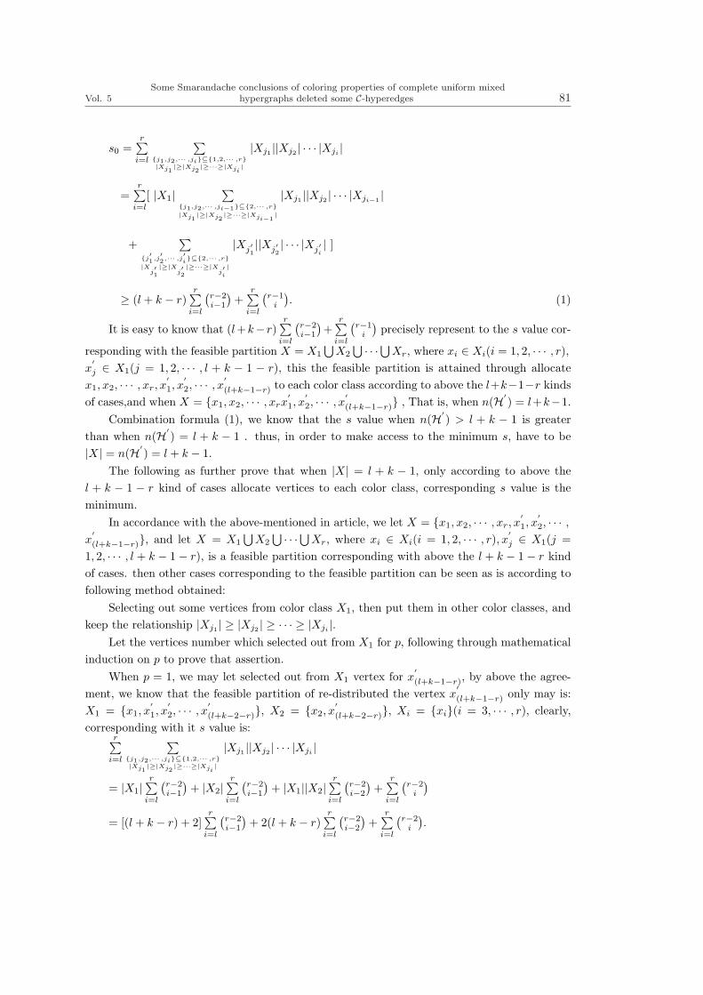
Vol. 5Some Smarandache conclusions of coloring properties of complete uniform mixed
hypergraphs deleted some C-hyperedges 81
s0 =r∑
i=l
∑j1,j2,··· ,ji⊆1,2,··· ,r|Xj1
|≥|Xj2|≥···≥|Xji
|
|Xj1 ||Xj2 | · · · |Xji|
=r∑
i=l
[ |X1|∑
j1,j2,··· ,ji−1⊆2,··· ,r|Xj1
|≥|Xj2|≥···≥|Xji−1
|
|Xj1 ||Xj2 | · · · |Xji−1 |
+∑
j′1,j′2,··· ,j
′i⊆2,··· ,r
|Xj′1|≥|X
j′2|≥···≥|X
j′i
|
|Xj′1||Xj
′2| · · · |Xj
′i| ]
≥ (l + k − r)r∑
i=l
(r−2i−1
)+
r∑i=l
(r−1
i
). (1)
It is easy to know that (l+k− r)r∑
i=l
(r−2i−1
)+
r∑i=l
(r−1
i
)precisely represent to the s value cor-
responding with the feasible partition X = X1
⋃X2
⋃ · · ·⋃ Xr, where xi ∈ Xi(i = 1, 2, · · · , r),x′j ∈ X1(j = 1, 2, · · · , l + k − 1 − r), this the feasible partition is attained through allocate
x1, x2, · · · , xr, x′1, x
′2, · · · , x
′(l+k−1−r) to each color class according to above the l+k−1−r kinds
of cases,and when X = x1, x2, · · · , xrx′1, x
′2, · · · , x
′(l+k−1−r) , That is, when n(H′
) = l+k−1.Combination formula (1), we know that the s value when n(H′
) > l + k − 1 is greaterthan when n(H′
) = l + k − 1 . thus, in order to make access to the minimum s, have to be|X| = n(H′
) = l + k − 1.The following as further prove that when |X| = l + k − 1, only according to above the
l + k − 1 − r kind of cases allocate vertices to each color class, corresponding s value is theminimum.
In accordance with the above-mentioned in article, we let X = x1, x2, · · · , xr, x′1, x
′2, · · · ,
x′(l+k−1−r), and let X = X1
⋃X2
⋃ · · ·⋃ Xr, where xi ∈ Xi(i = 1, 2, · · · , r), x′j ∈ X1(j =
1, 2, · · · , l + k − 1 − r), is a feasible partition corresponding with above the l + k − 1 − r kindof cases. then other cases corresponding to the feasible partition can be seen as is according tofollowing method obtained:
Selecting out some vertices from color class X1, then put them in other color classes, andkeep the relationship |Xj1 | ≥ |Xj2 | ≥ · · · ≥ |Xji
|.Let the vertices number which selected out from X1 for p, following through mathematical
induction on p to prove that assertion.When p = 1, we may let selected out from X1 vertex for x
′(l+k−1−r), by above the agree-
ment, we know that the feasible partition of re-distributed the vertex x′(l+k−1−r) only may is:
X1 = x1, x′1, x
′2, · · · , x
′(l+k−2−r), X2 = x2, x
′(l+k−2−r), Xi = xi(i = 3, · · · , r), clearly,
corresponding with it s value is:r∑
i=l
∑j1,j2,··· ,ji⊆1,2,··· ,r|Xj1
|≥|Xj2|≥···≥|Xji
|
|Xj1 ||Xj2 | · · · |Xji |
= |X1|r∑
i=l
(r−2i−1
)+ |X2|
r∑i=l
(r−2i−1
)+ |X1||X2|
r∑i=l
(r−2i−2
)+
r∑i=l
(r−2
i
)
= [(l + k − r) + 2]r∑
i=l
(r−2i−1
)+ 2(l + k − r)
r∑i=l
(r−2i−2
)+
r∑i=l
(r−2
i
).

82 Guobiao Zheng No. 3
In addition, it is clear that the l+k−1−r kinds of cases corresponding to the feasible Parti-tion X = X1
⋃X2
⋃ · · ·⋃ Xr, where xi ∈ Xi(i = 1, 2, · · · , r), x′j ∈ X1(j = 1, 2, · · · , l+k−1−r)
corresponding s value is:
r∑i=l
∑j1,j2,··· ,ji⊆1,2,··· ,r|Xj1
|≥|Xj2|≥···≥|Xji
|
|Xj1 ||Xj2 | · · · |Xji|
= |X1|r∑
i=l
(r−2i−1
)+
r∑i=l
(r−1
i
)
= (l + k − r)r∑
i=l
(r−2i−1
)+
r∑i=l
(r−1
i
).
It is clear that
[(l + k − r) + 2]r∑
i=l
(r − 2i− 1
)≥ (l + k − r)
r∑
i=l
(r − 2i− 1
),
2(l + k − r)r∑
i=l
(r − 2i− 2
)+
r∑
i=l
(r − 2
i
)≥
r∑
i=l
(r − 1
i
),
As a result,
[(l + k − r) + 2]r∑
i=l
(r − 2i− 1
)+ 2(l + k − r)
r∑
i=l
(r − 2i− 2
)+
r∑
i=l
(r − 2
i
)
≥ (l + k − r)r∑
i=l
(r − 2i− 1
)+
r∑
i=l
(r − 1
i
).
That is, when p = 1, the conclusion is true.
Assumption that when p < t the conclusions also are true. Then when p = t, that is,from the color class X1 select out t vertices re-assigned to other color classes and to maintainrelations |Xj1 | ≥ |Xj2 | ≥ · · · ≥ |Xji
|.We may let that the t time selected out from X1 vertex is x
′(l+k−t−r), and it will be
re-assigned to the color class Xj . And let this color classes X2, · · · , Xj−1, Xj , Xj+1, · · · , Xr
contained in the vertex total number different were: n2, · · · , nj−1, nj , nj+1, · · · , nr, at the sametime we let that this step operation before the color class X1 contained Vertices number forl + k− r− t + 1, then after the operation of this step each color class contained vertex numberdifferent are |X1| = l + k − r − t, |X2| = n2, · · · , |Xj−1| = nj−1, |Xj | = nj + 1, |Xj+1| =nj+1, · · · , |Xr| = nr.
It is easy to know s value corresponding with the feasible partition that obtained by afterthe t− 1 step operation is:
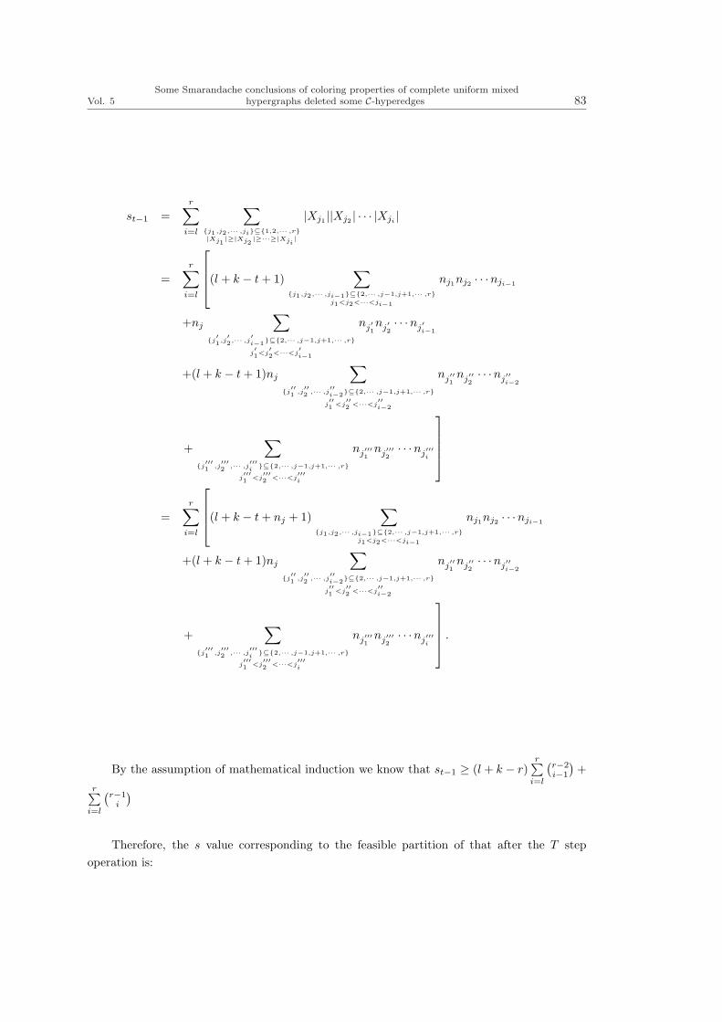
Vol. 5Some Smarandache conclusions of coloring properties of complete uniform mixed
hypergraphs deleted some C-hyperedges 83
st−1 =r∑
i=l
∑j1,j2,··· ,ji⊆1,2,··· ,r|Xj1
|≥|Xj2|≥···≥|Xji
|
|Xj1 ||Xj2 | · · · |Xji|
=r∑
i=l
(l + k − t + 1)
∑j1,j2,··· ,ji−1⊆2,··· ,j−1,j+1,··· ,r
j1<j2<···<ji−1
nj1nj2 · · ·nji−1
+nj
∑
j′1,j′2,··· ,j
′i−1⊆2,··· ,j−1,j+1,··· ,rj′1<j
′2<···<j
′i−1
nj′1nj′2· · ·nj
′i−1
+(l + k − t + 1)nj
∑
j′′1 ,j
′′2 ,··· ,j
′′i−2⊆2,··· ,j−1,j+1,··· ,r
j′′1 <j
′′2 <···<j
′′i−2
nj′′1nj′′2· · ·nj
′′i−2
+∑
j′′′1 ,j
′′′2 ,··· ,j
′′′i⊆2,··· ,j−1,j+1,··· ,r
j′′′1 <j
′′′2 <···<j
′′′i
nj′′′1
nj′′′2· · ·nj
′′′i
=r∑
i=l
(l + k − t + nj + 1)
∑j1,j2,··· ,ji−1⊆2,··· ,j−1,j+1,··· ,r
j1<j2<···<ji−1
nj1nj2 · · ·nji−1
+(l + k − t + 1)nj
∑
j′′1 ,j
′′2 ,··· ,j
′′i−2⊆2,··· ,j−1,j+1,··· ,r
j′′1 <j
′′2 <···<j
′′i−2
nj′′1nj′′2· · ·nj
′′i−2
+∑
j′′′1 ,j
′′′2 ,··· ,j
′′′i⊆2,··· ,j−1,j+1,··· ,r
j′′′1 <j
′′′2 <···<j
′′′i
nj′′′1
nj′′′2· · ·nj
′′′i
.
By the assumption of mathematical induction we know that st−1 ≥ (l + k − r)r∑
i=l
(r−2i−1
)+
r∑i=l
(r−1
i
)
Therefore, the s value corresponding to the feasible partition of that after the T stepoperation is:

84 Guobiao Zheng No. 3
st =r∑
i=l
∑j1,j2,··· ,ji⊆1,2,··· ,r|Xj1
|≥|Xj2|≥···≥|Xji
|
|Xj1 ||Xj2 | · · · |Xji|
=r∑
i=l
(l + k − t)
∑j1,j2,··· ,ji−1⊆2,··· ,j−1,j+1,··· ,r
j1<j2<···<ji−1
nj1nj2 · · ·nji−1
+(nj + 1)∑
j′1,j′2,··· ,j
′i−1⊆2,··· ,j−1,j+1,··· ,rj′1<j
′2<···<j
′i−1
nj′1nj′2· · ·nj
′i−1
+(l + k − t)(nj + 1)∑
j′′1 ,j
′′2 ,··· ,j
′′i−2⊆2,··· ,j−1,j+1,··· ,r
j′′1 <j
′′2 <···<j
′′i−2
nj′′1nj′′2· · ·nj
′′i−2
+∑
j′′′1 ,j
′′′2 ,··· ,j
′′′i⊆2,··· ,j−1,j+1,··· ,r
j′′′1 <j
′′′2 <···<j
′′′i
nj′′′1
nj′′′2· · ·nj
′′′i
=r∑
i=l
(l + k − t + nj + 1)
∑j1,j2,··· ,ji−1⊆2,··· ,j−1,j+1,··· ,r
j1<j2<···<ji−1
nj1nj2 · · ·nji−1
+(l + k − t + 1)nj
∑
j′′1 ,j
′′2 ,··· ,j
′′i−2⊆2,··· ,j−1,j+1,··· ,r
j′′1 <j
′′2 <···<j
′′i−2
nj′′1nj′′2· · ·nj
′′i−2
+∑
j′′′1 ,j
′′′2 ,··· ,j
′′′i⊆2,··· ,j−1,j+1,··· ,r
j′′′1 <j
′′′2 <···<j
′′′i
nj′′′1
nj′′′2· · ·nj
′′′i
+(l + k − t− nj)∑
j′′1 ,j
′′2 ,··· ,j
′′i−2⊆2,··· ,j−1,j+1,··· ,r
j′′1 <j
′′2 <···<j
′′i−2
nj′′1nj′′2· · ·nj
′′i−2
= st−1 + (l + k − t− nj)∑
j′′1 ,j
′′2 ,··· ,j
′′i−2⊆2,··· ,j−1,j+1,··· ,r
j′′1 <j
′′2 <···<j
′′i−2
nj′′1nj′′2· · ·nj
′′i−2
≥ (l + k − r)r∑
i=l
(r − 2i− 1
)+
r∑
i=l
(r − 1
i
)
+(l + k − t− nj)∑
j′′1 ,j
′′2 ,··· ,j
′′i−2⊆2,··· ,j−1,j+1,··· ,r
j′′1 <j
′′2 <···<j
′′i−2
nj′′1nj′′2· · ·nj
′′i−2
.
According to the agreement given when begin prove,after t step operation,the vertices‘number which contained in color class X1 is l + k − r − t, and it is not less than that any othercolor classes contained, namely l+k−r− t ≥ nj +1. Then l+k− t−nj ≥ t+1 > 0. Therefore,

Vol. 5Some Smarandache conclusions of coloring properties of complete uniform mixed
hypergraphs deleted some C-hyperedges 85
the feasible partition of that obtained after the t step operation corresponding value of s is
st ≥ (l + k − r)r∑
i=l
(r − 2i− 1
)+
r∑
i=l
(r − 1
i
).
That is, when p = t, the conclusions are true.Overview above, we know that the conclusions are true for any natural number p.In the following we prove this theorem conclusions on the basis of above assertion, It is
clear that by the assertion we the easy access to the following conclusions:1) When χ(H′
) = l, by the assertion we know that when the n(H′) = l + k− 1, s value is
the minimum and smin = k; if the vertices number n(H′) > l + k − 1, then s > k.
2) When n(H′) ≥ l + k − 1 and it is a definite value, and χ(H′
) > l, by above assertion,We know that the value of s corresponding to this condition certainly greater than k.
Combination of above two conclusions, we know that when l+k−1 ≤ |X| ≤ (l−1)(m−1),χ(H′
) ≥ l must have s > k.Again we return to the theorem proof. By the assumption χ(H′
) ≥ l of that given whenbegin prove conclusions from 3) and the known conditions l + k − 1 < |X| ≤ (l − 1)(m − 1),and combination proved just conclusion, we know s > k.
Because s represents the total number of C-stable set that is contained from one the feasiblepartition corresponding to a strict χ(H′
) ≥ l coloring of H′,and the cardinal number of C-stable
set is greater than l or equal to l, Because, each C-stable set which the cardinal number ofset is greater than l or equal to l contain at least one C-hyperedge of the mixed hypergraphH = (X,
(Xl
),(Xm
)). so mixed hypergraph H′
should does not contain at least s C-hyperedge,that is, |C′ | ≥ s > k, with known conditions |C′ | = k contradictions. Then, the assume isuntrue. Therefore, χ(H′
) ≤ l − 1.By above the whole process of prove, we know that when k ≥ 3, if l + k − 1 < |X| ≤
(l − 1)(m− 1), then χ(H′) = l − 1.
Corollary. Let H′= (X,
(Xl
) − C′ , (Xm
)), where C′ ⊆ (
Xl
), and let |C′ | = k, and s be the
number of C-stable set of H′, then
smin = (l + k − r)r∑
i=l
(r − 2i− 1
)+
r∑
i=l
(r − 1
i
)+
l−1∑
i=1
(n
i
)
where n = |X|.Proof. C-stable set of H′
is divided into two groups: one is those the cardinal number lessthan l; the other is those the cardinal number not less than l. By the above assertion and itsproof we know that the total number of C-stable set those cardinal number not less than l at
least equal to (l + k− r)r∑
i=l
(r−2i−1
)+
r∑i=l
(r−1
i
). It is easy obtain that total number of C-stable set
those the cardinal number less than l isl−1∑i=1
(ni
), so,
smin = (l + k − r)r∑
i=l
(r − 2i− 1
)+
r∑
i=l
(r − 1
i
)+
l−1∑
i=1
(n
i
).

86 Guobiao Zheng No. 3
References
[1] J. G. Yu, K. F. Diao, G.Z. Liu, On the minimum number of Edges of 4-Uinform C-hypergragh, Jinan, Shandong, Juornal of Shandong University, Science Edition, 38(2003), No.5, 56-60.
[2][5][6][9][10][11][12][13][16][18] Vitaly I. Voloshin, Coloring Mixed Hypergraphs Theory,Algorithms and Applications, American Mathematical Society Providence, Rhode Island, 2003.
[3] V. I. Voloshin, The mixed hypergraphs, Comput. Sci. J. Moldova, 1(1993), 45-52.[4][7] V. I. Voloshin, On the upper chromatic number of a hypergraph, Preprint of Moldova
State University, 1992.[6][8] V. I. Voloshin, On the upper chromatic number of a hypergraph, Scientific research
conference of Moldova State University, Abstracts of reports, Part 1, Moldova State University,42(1992).
[9] Zs. Tuza, V. I. Voloshin, Uncolorable mixed hypergraphs, Discrete Appl. Math.,99(2000), 209-227.
[14][15] G. B. Zheng, On the Upper and Lower Chromatic Number of One Type of UniformMixed Hypergraph, Journal of Qinghai Normal, 5(2007), 18-22.
[17] S. L. Song, Y. L. Xu, Combinatorial Mathematics Introduction, Print of ChineseScience Press, Beijing, 1999, 1-25.
[19] G. B. Zheng, Some Conclusions of the Chromatic Number of Complete Uniform MixedHypergraph Deleted about a Number of C-Hyperedges, Journal of Qinghai Normal, 5(2008),12-15.

Scientia MagnaVol. 5 (2009), No. 3, 87-90
A limit problem of the Smarandache dualfunction S∗∗(n)1
Qiuhong Zhao† and Yang Wang‡
†Department of Mathematics, Northwest University, Xi’an, Shaanxi, P.R.China‡College of Mathematics and Statistics, Nanyang Normal University,
Nanyang, Henan, P.R.China
Abstract For any positive integer n, the Smarandache dual function S∗∗(n) is defined as
S∗∗(n) =
max 2m : m ∈ N∗, (2m)!! | n , 2 | n;
max 2m− 1 : m ∈ N∗, (2m− 1)!! | n , 2 - n.
The main purpose of this paper is using the elementary methods to study the convergent
properties of an infinity series involving S∗∗(n), and give an interesting limit formula for it.
Keywords The Smarandache dual function, limit problem, elementary method.
§1. Introduction and Results
For any positive integer n, the Smarandache dual function S∗∗(n) is defined as the greatestpositive integer 2m − 1 such that (2m − 1)!! divide n, if n is an odd number; S∗∗(n) is thegreatest positive 2m such that (2m)!! divides n, if n is an even number. From the definition ofS∗∗(n) we know that the first few values of S∗∗(n) are: S∗∗(1) = 1, S∗∗(2) = 2, S∗∗(3) = 3,S∗∗(4) = 2, S∗∗(5) = 1, S∗∗(6) = 2, S∗∗(7) = 1, S∗∗(8) = 4, · · · . About the elementaryproperties of S∗∗(2), some authors had studied it, and obtained many interesting results. For
example, Su Gou [1] proved that for any real number s > 1, the series∞∑
n=1
S∗∗(n)ns is absolutely
convergent, and
∞∑n=1
S∗∗(n)ns
= ζ(s)(
1− 12s
) (1 +
∞∑m=1
2((2m + 1)!!)s
)+ ζ(s)
( ∞∑m=1
2((2m)!!)s
),
where ζ(s) is the Riemann zeta-function.
Yanting Yang [2] studied the mean value estimate of S∗∗(n), and gave an interesting asymp-totic formula: ∑
n≤x
S∗∗(n) = x
(2e
12 − 3 + 2e
12
∫ 1
0
e−y2
2 dy
)+ O(ln2 x),
where e = 2.7182818284 · · · is a constant.1This work is supported by the Shaanxi Provincial Education Department Foundation 08JK433.

88 Qiuhong Zhao and Yang Wang No. 3
Yang Wang [3] also studied the mean value properties of S∗∗(n)2, and prove that
∑
n≤x
S∗∗(n)2 =13x
2+ O
((lnx
ln lnx
)3)
.
In this paper, we using the elementary method to study the convergent properties of the series
∞∑n=1
S∗∗(n)2
ns,
and give an interesting identity and limit theorem. That is, we shall prove the following:Theorem. For any real number s > 1, we have the identity
∞∑n=1
S∗∗(n)2
ns= ζ(s)
[1− 1
2s+
(1− 1
2s
) ∞∑m=1
8m
((2m + 1)!!)s+
∞∑m=1
8m− 4((2m)!!)s
],
where ζ(s) is the Riemann zeta-function.
From this Theorem we may immediately deduce the following limit formula:
Corollary. We have the limit
lims→1
(s− 1)
( ∞∑n=1
S∗∗(n)2
ns
)=
132
.
§2. Proof of the theorem
In this section, we shall complete the proof of our theorem directly. It is clear that S∗∗(n) ¿lnn, so if s > 1, then the series
∞∑n=1
S∗∗(n)2
ns is convergent absolutely, so we have
∞∑n=1
S∗∗(n)2
ns=
∞∑n=12-n
S∗∗(n)2
ns+
∞∑n=12|n
S∗∗(n)2
ns≡ S1 + S2,
where
S1 =∞∑
n=12-n
S∗∗(n)2
ns, S2 =
∞∑n=12|n
S∗∗(n)2
ns.
From the definition of S∗∗(n) we know that if 2 - n, we can assume that S∗∗(n) = 2m− 1, then(2m− 1)!! | n. Let n = (2m− 1)!!u, 2m + 1 - u. Note that the identity
∞∑n=1
1(2n− 1)s
=∞∑
n=1
1ns−
∞∑n=1
1(2n)s
=(
1− 12s
) ∞∑n=1
1ns
=(
1− 12s
)ζ(s),

Vol. 5 A limit problem of the Smarandache dual function S∗∗(n) 89
so from the definition of S∗∗(n) we can deduce that ( s > 1 ),
S1 =∞∑
m=1
∞∑
u=1, 2-u2m+1-u
(2m− 1)2
((2m− 1)!!)sus
=∞∑
m=1
(2m− 1)2
((2m− 1)!!)s
∞∑
u=1, 2-u2m+1-u
1us
=∞∑
m=1
(2m− 1)2
((2m− 1)!!)s
( ∞∑n=1
1(2n− 1)s
− 1(2m + 1)s
∞∑n=1
1(2n− 1)s
)
= ζ(s)(
1− 12s
) ( ∞∑m=1
(2m− 1)2
((2m− 1)!!)s−
∞∑m=1
(2m− 1)2
((2m + 1)!!)s
)
= ζ(s)(
1− 12s
) (1 +
∞∑m=1
(2m + 1)2 − (2m− 1)2
((2m + 1)!!)s
)
= ζ(s)(
1− 12s
) (1 +
∞∑m=1
8m
((2m + 1)!!)s
).
For even number n, we assume that S∗∗(n) = 2m, then (2m)!! | n. Let n = (2m)!!v, 2m+2 - v.If s > 1, then we can deduce that
S2 =∞∑
m=1
∞∑v=1
2m+2-v
(2m)2
((2m)!!)svs
=∞∑
m=1
(2m)2
((2m)!!)s
∞∑v=1
(2m+2)-v
1vs
=∞∑
m=1
(2m)2
((2m)!!)s
( ∞∑n=1
1ns− 1
(2m + 2)s
∞∑n=1
1ns
)
= ζ(s)
( ∞∑m=1
(2m)2
((2m)!!)s−
∞∑m=1
(2m)2
((2m + 2)!!)s
)
= ζ(s)
(1
2s−2+
∞∑m=1
(2m + 2)2 − (2m)2
((2m + 2)!!)s
)
= ζ(s)
(1
2s−2+
∞∑m=1
8m + 4((2m + 2)!!)s
)
= 4ζ(s)∞∑
m=1
2m− 1((2m)!!)s
.
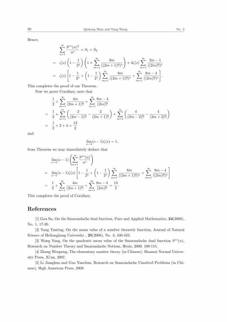
90 Qiuhong Zhao and Yang Wang No. 3
Hence,∞∑
n=1
S∗∗(n)2
ns= S1 + S2
= ζ(s)(
1− 12s
) (1 +
∞∑m=1
8m
((2m + 1)!!)s
)+ 4ζ(s)
∞∑m=1
2m− 1((2m)!!)s
= ζ(s)
[1− 1
2s+
(1− 1
2s
) ∞∑m=1
8m
((2m + 1)!!)s+
∞∑m=1
8m− 4((2m)!!)s
].
This completes the proof of our Theorem.Now we prove Corollary, note that
12
+∞∑
m=1
4m
(2m + 1)!!+
∞∑m=1
8m− 4(2m)!!
=12
+∞∑
m=1
(2
(2m− 1)!!− 2
(2m + 1)!!
)+
∞∑m=1
(4
(2m− 2)!!− 4
(2m + 2)!!
)
=12
+ 2 + 4 =132
and
lims→1
(s− 1)ζ(s) = 1,
from Theorem we may immediately deduce that
lims→1
(s− 1)
( ∞∑n=1
S∗∗(n)ns
)
= lims→1
(s− 1)ζ(s)
[1− 1
2s+
(1− 1
2s
) ∞∑m=1
8m
((2m + 1)!!)s+
∞∑m=1
8m− 4((2m)!!)s
]
=12
+∞∑
m=1
4m
(2m + 1)!!+
∞∑m=1
8m− 4(2m)!!
=132
.
This completes the proof of Corollary.
References
[1] Gou Su, On the Smarandache dual function, Pure and Applied Mathematics, 24(2008),No. 1, 17-20.
[2] Yang Yanting, On the mean value of a number theoretic function, Journal of NaturalScience of Heilongjiang University , 25(2008), No. 3, 340-342.
[3] Wang Yang, On the quadratic mean value of the Smarandache dual function S∗∗(n),Research on Number Theory and Smarandache Notions, Hexis, 2009, 109-115.
[4] Zhang Wenpeng, The elementary number theory (in Chinese), Shaanxi Normal Univer-sity Press, Xi’an, 2007.
[5] Li Jianghua and Guo Yanchun, Research on Smarandache Unsolved Problems (in Chi-nese), High American Press, 2009.

Scientia MagnaVol. 5 (2009), No. 3, 91-99
Separation axioms in smooth fuzzy topologicalspaces
B. Amudhambigai, M. K. Uma and E. Roja
Department of Mathematics Sri Sarada College for Women, Salem-16 Tamil Nadu, IndiaE-mail: [email protected]
Abstract In this paper, the concepts of fuzzy∼g −Ti (i = 0, 1, 2, 1/2) spaces, fuzzy
∼g-normal
spaces and fuzzy∼g-regular spaces in the sense of Sostak [7] are introduced. Also, some
interesting properties and characterizations of them are investigated.
Keywords Fuzzy∼g −Ti (i = 0, 1, 2, 1/2) spaces, fuzzy
∼g-normal spaces, fuzzy
∼g-regular
spaces.
§1. Introduction and Preliminaries
The concept of fuzzy set was introduced by Zadeh [10] in his classical paper. Fuzzy setshave applications in many fields such as information [6] and control [8]. In 1985, Sostak [7]introduced a new form of topological structure. In 1992, Ramadan [4] studied the concept ofsmooth fuzzy topological spaces. The concept of
∼g-open set was discussed by Rajesh and Erdal
Ekici [3]. The concept of fuzzy normal spaces was introduced by Bruce Hutton [1]. Kubiak [9]established many interesting properties of fuzzy normal spaces. The purpose of this paper is tointroduce fuzzy
∼g −Ti (i = 0, 1, 2, 1/2) spaces,
∼g-normality and
∼g-regularity in smooth fuzzy
topological spaces. Also many interesting characterizations are established.Throughout this paper, let X be a nonempty set, I = [0, 1] and I0 = (0, 1]. For 〈∈ I,
T (x) = 〈 for all x ∈ X.Definition 1.1. [2] A fuzzy point xt in X is a fuzzy set taking value t ∈ I0 at x and zero
elsewhere, xt ∈ λ iff t ≤ λ(x). A fuzzy set λ is quasi-coincident with a fuzzy set µ, denoted byλ q µ, if there exists x ∈ X such that λ(x) + µ(x) > 1. Otherwise λ q µ.
Definition 1.2. [7] A function T : IX → I is called a smooth fuzzy topology on X if itsatisfies the following conditions :(1) T (0) = T (1) = 1;(2) T (µ1 ∧ µ2) ≥ T (µ1) ∧ T (µ2) for any µ1, µ2 ∈ IX .(3) T ( ∨
j ∈ Γµj) ≥ ∧
j ∈ ΓT (µj) for any µj j ∈ Γ ∈ IX.
The pair (X, T ) is called a smooth fuzzy topological space.Remark 1.1. Let (X, T ) be a smooth fuzzy topological space. Then, for each r ∈ I0, Tr =
µ ∈ IX : T (µ) ≥ r is Chang’s fuzzy topology on X.Definition 1.3. [5] Let (X, T ) be a smooth fuzzy topological space. For each λ ∈ IX , r ∈
I0, an operator CT : IX ×I0 → IX is defined as follows: CT (λ, r) = ∧µ : µ ≥ λ, T (1−µ) ≥ r.

92 B. Amudhambigai, M. K. Uma and E. Roja No. 3
For λ, µ ∈ IX and r, s ∈ I0, it satisfies the following conditions:(1) CT (0, r) = 0.(2) λ ≤ CT (λ, r).(3) CT (λ, r) ∨ CT (µ, r) = CT (λ ∨ µ, r).(4) CT (λ, r) ≤ CT (λ, s), if r ≤ s.
(5) CT (CT (λ, r), r) = CT (λ, r).Proposition 1.1. [5] Let (X, T ) be a smooth fuzzy topological space. For each λ ∈ IX ,
r ∈ I0, an operator IT : IX × I0 → IX is defined as follows: IT (λ, r) = ∨µ : µ ≤ λ, T (µ) ≥ r.For λ, µ ∈ IX and r, s ∈ I0, it satisfies the following conditions:(1) IT (1− λ, r) = 1− CT (λ, r).(2) IT (1, r) = 1.
(3) λ ≥ IT (λ, r).(4) IT (λ, r) ∧ IT (µ, r) = IT (λ ∧ µ, r).(5) IT (λ, r) ≥ IT (λ, s), ifr ≤ s.
(6) IT (IT (λ, r), r) = IT (λ, r).Definition 1.4. [4] Let (X, T ) be a smooth fuzzy topological space. For λ ∈ IX and
r ∈ I0,(1) SCT (λ, r) = ∧µ ∈ IX : µ ≥ λ, µ is r− fuzzy semiclosed is called r-fuzzy semiclosure of λ.(2) λ is called r-fuzzy semiclosed (briefly, r-fsc) if λ ≥ IT (CT (λ, r), r).(3) λ is called r-fuzzy semiopen (briefly, r-fso) if λ ≤ CT (IT (λ, r), r).
Definition 1.5. [4] Let (X, T ) and (Y, S) be any two smooth fuzzy topological spaces.Let f : (X, T ) → (Y, S) be a function. Then(1) f is called fuzzy continuous iff S(µ) ≤ T (f−1(µ)) for each µ ∈ IY .
(2) f is called fuzzy open iff T (λ) ≤ S(f(λ)) for each λ ∈ IX .
§2. Fuzzy∼g−Ti spaces
In this section, the concept of fuzzy∼g −Ti (i = 0, 1, 2, 1/2) spaces is introduced. Interesting
properties and characterizations of such spaces are discussed.Definition 2.1. Let (X, T) be a smooth fuzzy topological space. For λ ∈ IX and r ∈ I0,
λ is called(1) r-fuzzy
∧g-closed if CT (λ, r) ≤ µ whenever λ ≤ µ and µ is r-fuzzy semiopen. The complement
of a r-fuzzy∧g-closed set is said to be a r-fuzzy
∧g-open set.
(2) r-fuzzy *g-closed if CT (λ, r) ≤ µ whenever λ ≤ µ and µ is r-fuzzy∧g-open. The complement
of a r-fuzzy *g-closed set is said to be a r-fuzzy *g-open set.(3) r-fuzzy #g-semiclosed (briefly r-#fgs-closed) if SCT (λ, r) ≤ µ whenever λ ≤ µ and µ isr-fuzzy *g-open. The complement of a r-fuzzy #g-semiclosed set is said to be a r-fuzzy #g-semiopen set (briefly r-#fgs-open set ).(4) r-fuzzy
∼g-closed if CT (λ, r) ≤ µ whenever λ ≤ µ and µ is r-#fgs-open. The complement of
a r-fuzzy∼g-closed set is said to be a r-fuzzy
∼g-open set.
Definition 2.2. Let (X, T ) be a smooth fuzzy topological space. For λ ∈ IX and r ∈ I0,(1)
∼g −IT (λ, r) = ∨µ ∈ IX : µ ≤ λ, µ is a r− fuzzy
∼g −openset is called r-fuzzy
∼g-interior of

Vol. 5 Separation axioms in smooth fuzzy topological spaces 93
λ.(2)
∼g −CT (λ, r) = ∧µ ∈ IX : µ ≥ λ, µ is a r− fuzzy
∼g −closedset is called r-fuzzy
∼g-closure
of λ.
Definition 2.3. Let (X, T ) be a smooth fuzzy topological space. For λ ∈ IX and r ∈ I0,λ is called r-generalized fuzzy
∼g-closed (briefly, r-gf
∼g-closed) iff
∼g −CT (λ, r) ≤ µ whenever
λ ≤ µ, µ ∈ IX is r-fuzzy∼g-open. The complement of a r-generalized fuzzy
∼g-closed set is a
r-generalized fuzzy∼g-open set ( briefly, r-gf
∼g-open ).
Definition 2.4. Let (X, T ) and (Y, S) be any two smooth fuzzy topological spaces. Letf : (X, T ) → (Y, S) be a function.(1) f is called
∼g-open ( resp.
∼g-closed ) if for each r-fuzzy
∼g-open set λ ∈ IX , f(λ) ∈ IY is
r-fuzzy∼g-open ( resp. r-fuzzy
∼g-closed ).
(2) f is called∼g-continuous if for each λ ∈ IY with S(λ) ≥ r, f−1(λ) ∈ IX is r-fuzzy
∼g-open.
(3) f is called fuzzy∼g-irresolute if for each r-fuzzy
∼g-open set λ ∈ IY , f−1(λ) ∈ IX is r-fuzzy
∼g-open.(4) f is called fuzzy
∼g-homeomorphism if f is one to one, onto, fuzzy
∼g-irresolute and fuzzy
∼g-open.(5) f is called gf
∼g-irresolute if for each r-gf
∼g closed set λ ∈ IY , f−1(λ) ∈ IX is r-gf
∼g-closed.
(6) f is called gf∼g-closed iff for any r-gf
∼g-closed set λ ∈ IX , f(λ) is r- gf
∼g-closed.
Definition 2.5. A smooth fuzzy topological space (X, T ) is called(1) Fuzzy
∼g −To iff for λ, µ ∈ IX with λ q µ, there exists r-fuzzy
∼g-open set δ ∈ IX such that
either λ ≤ δ or µ ≤ δ, λ q δ.(2) Fuzzy
∼g −T1 iff for λ, µ ∈ IX with λ q µ, there exist r-fuzzy
∼g-open sets δ, η ∈ IX such
that either λ ≤ δ, µ q δ or µ ≤ η, λ q η.(3) Fuzzy
∼g −T2 iff for λ, µ ∈ IX with λ q µ, there exist r-fuzzy
∼g-open sets δ, η ∈ IX with λ
≤ δ, µ ≤ η and δ q η.(4) Fuzzy
∼g −R0 iff λ q
∼g −CT (µ, r) implies that µ q
∼g −CT (λ, r) for λ, µ ∈ IX .
Definition 2.6. A smooth fuzzy topological space (X, T ) is called fuzzy∼g −T1/2 if every
r - gf∼g-closed set is r-fuzzy
∼g- closed.
Proposition 2.1. Let (X, T ) be a smooth fuzzy topological space. For r ∈ I0, the followingproperties hold:(i) For all r-fuzzy
∼g- open set λ ∈ IX , λ q µ iff λ q (
∼g −CT (µ, r)), µ ∈ IX .
(ii) δ q (∼g −CT (λ, r)) iff λ q µ for all r-fuzzy
∼g -open set µ ∈ IX with δ ≤ µ, for λ, δ ∈ IX .
Proof. (i) Let λ be a r-fuzzy∼g-open set such that λ q µ. Since µ ≤ ∼
g −CT (µ, r), λ
q∼g CT (µ, r). Conversely let λ be a r-fuzzy
∼g-open set such that λ q µ. Then µ ≤ 1 − λ,
this implies that∼g −CT (µ, r) ≤ ∼
g −CT (1 − λ, r) = 1 − λ. Now,∼g −CT (µ, r) ≤ 1 − λ. Thus
λ q∼g −CT (µ, r) which is a contradiction. Hence the result.
(ii) Let δ q (∼g −CT (λ, r)). Since δ ≤ µ, µ q (
∼g −CT (λ, r)). By ( i ), µ q λ for all r-fuzzy
∼g-
open set µ with δ ≤ µ. Conversely suppose that δ q∼g −CT (λ, r). Then δ ≤ 1− (
∼g −CT (λ, r)).
Let µ = 1 − (∼g −CT (µ, r)) . Then µ is a r-fuzzy
∼g-open set. Since λ ≤ ∼
g −CT (λ, r), µ =1− (
∼g −CT (λ, r)) ≤ 1− λ, this implies that λ q µ, a contradiction. Hence the result.
Proposition 2.2. Let ( X, T ) be a smooth fuzzy topological space. For δ, ρ ∈ IX , thefollowing statements are equivalent:

94 B. Amudhambigai, M. K. Uma and E. Roja No. 3
(i) (X, T ) is fuzzy∼g −R0.
(ii) If δ q λ =∼g −CT (λ, r), λ ∈ IX and r ∈ I0, there exists a r-fuzzy
∼g-open set µ such that
δ q µ and λ ≤ µ.(iii) If δ q λ =
∼g −CT (λ, r), then
∼g −CT (δ, r) q λ =
∼g −CT (λ, r), λ ∈ IX and r ∈ I0.
(iv) If δ q∼g −CT (ρ, r) then
∼g −CT (δ, r) q
∼g −CT (ρ, r), r ∈ I0.
Proof. (i) ⇒ (ii) Let δ q λ =∼g −CT (λ, r). Since
∼g −CT (ρ, r) ≤ ∼
g −CT (λ, r) for each ρ ≤λ, we have δ q (
∼g −CT (ρ, r)). By ( i ), ρ q (
∼g −CT (δ, r)). By ( ii ) of Proposition 2.1, for each
ρ q (∼g −CT (δ, r)), there exists a r-fuzzy
∼g-open set η such that δ q η, ρ ≤ η. Let µ= ∨ η:
δ q η . Then δ q µ, λ ≤ µ for all r-fuzzy∼g-open set µ.
(ii) ⇒ (iii) Let δ q λ =∼g −CT (λ, r). By ( ii ), there exists a r-fuzzy
∼g-open set µ ∈ IX
such that δ q µ and λ ≤ µ. Since δ q µ, it follows that δ ≤ 1 − µ. This implies that∼g −CT (δ, r) ≤ ∼
g −CT (1− µ, r) = 1− µ ≤ 1− λ. Hence∼g −CT (δ, r) q λ =
∼g −CT (λ, r).
(iii)⇒(iv) Let δ q∼g −CT (ρ, r). Since
∼g −CT (
∼g −CT (ρ, r), r) =
∼g −CT (ρ, r) and by ( iii ),
∼g −CT (δ, r) q
∼g −CT (ρ, r).
(iv)⇒ (i) Let δ q∼g −CT (ρ, r). By ( iv ),
∼g −CT (δ, r) q
∼g −CT (ρ, r). Since ρ ≤ ∼
g −CT (ρ, r),ρ q
∼g −CT (δ, r). Hence ( X, T ) is fuzzy
∼g −R0.
Proposition 2.3. Let ( X, T ) and ( Y, S) be any two smooth fuzzy topological spaces.Let f : (X, T ) → (Y, S) be a fuzzy
∼g-irresolute, gf
∼g-irresolute and fuzzy
∼g-closed function.
Then the following conditions hold:(i) If f is injective and (Y, S ) is a fuzzy
∼g −T1/2 space, then (X, T ) is a fuzzy
∼g −T1/2 space.
(ii) If f is surjective and (X, T ) is a fuzzy∼g −T1/2 space, then (Y, S) is a fuzzy
∼g −T1/2 space.
Proof. (i) Let λ ∈ IX be a r-gf∼g-closed set. Since f is gf
∼g-closed, f ( λ ) ∈ IY is r-gf
∼g-
closed. Since (Y, S) is fuzzy∼g −T1/2, f(λ) is r-fuzzy
∼g-closed. Now, λ = f−1(f(λ)) is r-fuzzy
∼g-closed. Hence (X, T ) is a fuzzy
∼g −T1/2 space.
(ii) Let µ ∈ IY be a r-gf∼g-closed set. Since f is gf
∼g-irresolute, f−1(µ) ∈ IX is a r-gf
∼g-
closed set. Since (X, T ) is a fuzzy∼g −T1/2 space, f−1(µ) is a r-fuzzy
∼g-closed set. Therefore
µ = f(f−1(µ)) is r-fuzzy∼g-closed. Hence (Y, S) is a fuzzy
∼g −T1/2 space.
Proposition 2.4. Let ( X, T ) and (Y, S ) be any two smooth fuzzy topological spaces.Let f : (X, T ) → (Y, S) be a fuzzy
∼g-irresolute, and injective function. If ( Y, S) is fuzzy
∼g −T2
( resp. fuzzy∼g −T1 ), then ( X, T ) is fuzzy
∼g −T2 ( resp. fuzzy
∼g −T1 ).
Proof. Let ( Y, S) be a fuzzy∼g −T2 space. Let λ1, λ2 ∈ IX be such that λ1 q λ2, then
exist r-fuzzy∼g-open sets λ, µ ∈ IY such that f(λ1) ≤ λ and f(λ2) ≤ µ such that λ q µ. Then
λ ≤ 1 − µ which implies that f−1(λ) q f−1(µ). Now, λ1 ≤ f−1(λ) and λ2 ≤ f−1(µ). Since f isfuzzy
∼g-irresolute, f−1(λ) and f−1(µ) are r-fuzzy
∼g-open sets. Hence ( X, T ) is a fuzzy
∼g −T2
space. Similarly we prove the case of fuzzy∼g −T1 space.
§3. Fuzzy∼g-normal spaces and its characterizations
In this section, the concept of fuzzy∼g-normal space is introduced. Interesting properties
and characterizations of such space are discussed.Definition 3.1. A smooth fuzzy topological space (X, T ) is said to be fuzzy
∼g-normal if
for every r-fuzzy∼g-closed set λ and r-fuzzy
∼g-open set µ with λ ≤ µ there exists a γ ∈ IX such

Vol. 5 Separation axioms in smooth fuzzy topological spaces 95
that λ ≤ ∼g −IT (γ, r) ≤ ∼
g −CT (γ, r) ≤ µ, r ∈ I0.
Proposition 3.1. For any smooth fuzzy topological space (X, T ) and λ, µ, δ ∈ IX , r ∈ I0,the following statements are equivalent:(i) (X, T ) is fuzzy
∼g-normal.
(ii) For each r-fuzzy∼g-closed set λ and each r-fuzzy
∼g-open set µ with λ ≤ µ, there exists a
r-fuzzy∼g-open set δ such that
∼g −CT (λ, r) ≤ δ ≤ ∼
g −CT (δ, r) ≤ µ.(iii) For each r-gf
∼g-closed set λ and r-fuzzy
∼g-open set µ with λ ≤ µ, there exists a r-fuzzy
∼g-open set δ such that
∼g −CT (λ, r) ≤ δ ≤ ∼
g −CT (δ, r) ≤ µ.
Proof. (i) ⇒ (ii) The proof is trivial.
(ii) ⇒ (iii) Let λ be any r-gf∼g-closed set and µ be any r-fuzzy
∼g-open set such that λ ≤ µ .
Since λ is r-gf∼g-closed,
∼g −CT (λ, r) ≤ µ. Now,
∼g −CT (λ, r) is r-fuzzy
∼g-closed and µ is r-fuzzy
∼g-
open. By ( ii ), there exists a r-fuzzy∼g-open set δ such that
∼g −CT (λ, r) ≤ δ ≤ ∼
g −CT (δ, r) ≤ µ.
(iii) ⇒ (i) The proof is trivial.
Proposition 3.2. Let (X, T ) and (Y, S ) be any two smooth fuzzy topological spaces.If f : (X, T ) → (Y, S) is fuzzy
∼g-homeomorphism and (Y, S) is fuzzy
∼g-normal, then (X, T ) is
fuzzy∼g-normal.
Proof. Let λ ∈ IX be any r-fuzzy∼g-closed set and µ ∈ IX be any r-fuzzy
∼g-open set such
that λ ≤ µ where r ∈ I0. Since f is fuzzy∼g-homeomorphism, it is also fuzzy
∼g-closed. Hence
f(λ) ∈ IY is r-fuzzy∼g-closed. Since f is fuzzy
∼g-open, f(µ) ∈ IY is r-fuzzy
∼g-open. Since (Y, S)
is fuzzy∼g-normal, there exists a γ ∈ IY such that f(λ) ≤ ∼
g −IT (γ, r) ≤ ∼g −CT (γ, r) ≤ f(µ).
Now, f−1(f(λ)) = λ ≤ f−1(∼g −IT (γ, r)) ≤ f−1(
∼g −CT (γ, r)) ≤ f−1(f(µ)) = µ. That is,
λ ≤ ∼g −IT (f−1(γ), r) ≤ ∼
g −CT (f−1(γ), r) ≤ µ. Therefore (X, T ) is fuzzy∼g-normal.
Proposition 3.3. Let (X, T ) and (Y, S) be any two smooth fuzzy topological spaces. Iff : (X, T ) → (Y, S) is fuzzy
∼g-homeomorphism and (X, T ) is a fuzzy
∼g-normal space, then (Y,
S) is fuzzy∼g-normal.
Proof. Let λ ∈ IY be any r-fuzzy∼g-closed set and µ ∈ IY be any r-fuzzy
∼g-open set
such that λ ≤ µ where r ∈ I0. Since f is fuzzy∼g-irresolute, f−1(λ) is r-fuzzy
∼g-closed and
f−1(µ) ∈ IY is r-fuzzy∼g-open. Since (X, T ) is fuzzy
∼g-normal, there exists a γ ∈ IX such
that f−1(λ) ≤ ∼g −IT (γ, r) ≤ ∼
g −CT (γ, r) ≤ f−1(µ). Now, f(f−1(λ)) = λ ≤ f(∼g −IT (γ, r)) ≤
f(∼g −CT (γ, r)) ≤ f(f−1(µ)) = µ. That is, λ ≤ ∼
g −IT (f(γ), r) ≤ ∼g −CT (f(γ), r) ≤ µ. There-
fore (Y, S) is fuzzy∼g-normal.
Proposition 3.4. Let (X, T ) be a smooth fuzzy topological space which is also a fuzzy∼g-normal space. Let λi i ∈ J∈ IX and µj j ∈ J ∈ IX . If there exist λ, µ ∈ IX such that∼g −CT (λi, r) ≤
∼g −CT (λ, r) ≤ ∼
g −IT (µj , r) and∼g −CT (λi, r) ≤
∼g −IT (µ, r) ≤ ∼
g −IT (µj , r) forall i, j = 1, 2, · · · , and r ∈ I0, then there exists γ ∈ IX such that
∼g −CT (λi, r) ≤
∼g −IT (γ, r) ≤ ∼
g −CT (γ, r) ≤ ∼g −IT (µj , r), for all i, j = 1, 2, · · · .
Proof. First, we shall show by induction that for all n ≥ 2 there exists a collectionγi, δi/1 ≤ i ≤ n contained in IX such that the conditions

96 B. Amudhambigai, M. K. Uma and E. Roja No. 3
∼g −CT (λi, r) ≤
∼g −IT (γi, r);
∼g −CT (δj , r) ≤
∼g −IT (µj , r);
∼g −CT (λ, r) ≤ ∼
g −IT (δj , r);∼g −CT (γi, r) ≤
∼g −IT (µ, r);
∼g −CT (γi, r) ≤
∼g −IT (δj , r),
(sn)
hold for all i, j = 1, 2, ....n − 1. Clearly (S2) follows at once from the fuzzy∼g-normality of
(X, T ). Now, suppose that for n ≥ 2, γi, δi ∈ IX(i < n) such that (Sn) holds. Since∼g −CT (λn, r) ≤ ∼
g −CT (λ, r) ≤ ∼g −IT (δj , r)(j < n) and
∼g −CT (λn, r) ≤ ∼
g −IT (µ, r) by fuzzy∼g-normality of (X, T ), there exists γn ∈ IX such that
∼g −CT (λn, r) ≤ ∼
g −IT (γn, r) ≤ ∼g −CT (γn, r) ≤ ∼
g −IT
(∧
j < nδj ∧ µ, r
).
Similarly, since∼g −CT (λ, r) ≤ ∼
g −IT (µn, r) and∼g −CT (γi, r) ≤
∼g −IT (µn, r)(i ≤ n), there
exists δn ∈ IX such that
(∨
i ≤ n
∼g −CT ( γi, r ) ∨ ∼
g −CT ( λ, r ))
≤ ∼g −IT (δn, r)
≤ ∼g −CT (δn, r)
≤ ∼g −IT (µn, r).
Thus (Sn+1) holds.Let γ =
∞∨i=1
γi. Then∼g −CT (λi, r) ≤
∼g −IT (γi, r) ≤
∼g −IT (γ, r) for all i = 1, 2, · · · . Since
∼g −CT (γi, r) ≤
∼g −IT (δj , r)(i, j = 1, 2, · · · ), γi ≤ δj , so that
∼g −CT (γ, r) ≤ ∼
g −CT (δj , r) ≤∼g −IT (µj , r) for all j = 1, 2, · · · . This proves the result.
Proposition 3.5. Let (X, T ) be a smooth fuzzy topological space which is also a fuzzy∼g-normal space. If λqq∈Q and µqq∈Q are monotone increasing collections of respectively,fuzzy
∼g-closed and fuzzy
∼g-open subsets of (X, T ) (Q is the set of all rational numbers ) such
that λq ≤ µs whenever q < s, then there exists a collection γqq∈Q ∈ IX such that
λq ≤∼g −IT (γs, r),
∼g −CT (γq, r) ≤
∼g −IT (γs, r) and
∼g −CT (γq, r) ≤ µs
whenever q < s.Proof. Let us arrange into a sequence qn of all rational numbers (without repetitions).
For every n ≥ 2 we shall define inductively a collection γqi/1 ≤ i ≤ n ∈ IX such that
λq ≤∼g −IT (γqi
, r), if q < qi;∼g −CT (γqi
, r) ≤ µq, if qi < q;∼g −CT (γqi , r) ≤
∼g −IT (γqj , r), if qi < qj ,
(sn)
for all 1 ≤ i, j < n. It is clear that the countable collections λq/q < q1 and µq/q > q1together with λq1 and µq1 satisfy all hypotheses of Proposition 3.4, so that there exists δ1 ∈ IX
such that λq ≤∼g −IT (δ1, r) for all q < q1 and
∼g −CT (δ1, r) ≤ µq for all q > q1.

Vol. 5 Separation axioms in smooth fuzzy topological spaces 97
Letting γq1 = δ1, we get (S2). Assume that the fuzzy subsets γqiare already defined for
i < n and satisfy (Sn). Define
λ = ∨γqi/i < n, qi < qn ∨ λqn and µ = ∧γqj /j < n, qj < qn ∧ µqn.
Then∼g −CT (γqi
, r) ≤ ∼g −CT (λ, r) ≤ ∼
g −IT (γqj, r), and
∼g −CT (γqi
, r) ≤ ∼g −IT (µ, r) ≤ ∼
g −IT (γqj, r)
whenever qi < qn < qj , (i, j < n) as well as λq ≤∼g −CT (λ, r) ≤ µs and λq ≤
∼g −IT (µ, r) ≤ µs
whenever q < qn < s. This shows that the countable collections γqi/i <, qi < qn∨λq/q < qnand γqj
/j < n, qj > qn ∨ µq/q > qn together with λ and µ satisfy all hypotheses of Propo-sition 3.5. Hence there exists a δn ∈ IX such that
λq ≤∼g −IT (δn, r), if q < qn
∼g −CT (γqi
, r) ≤ ∼g −IT (δn, r), if qi < qn
∼g −CT (δn, r) ≤ µq, if qn < q∼g −CT (δn, r) ≤ ∼
g −IT (γqj, r), if qn < qj
where 1 ≤ i, j ≤ n − 1. Letting γqn = δn we obtain fuzzy subsets γq1 , γq2 , · · · , γqn that satisfythe result (Sn+1). Therefore the collection γqi
/i = 1, 2, · · · . has the required properties. Thiscompletes the proof.
§4. Fuzzy∼g-regular space and its characterizations
In this section, the concept of fuzzy∼g-regular space is introduced. Some interesting char-
acterizations are established.Definition 4.1. A smooth fuzzy topological space (X, T ) is called a fuzzy
∼g-regular space
if for every r-fuzzy∼g-closed set λ and each α ∈ IX with α λ, there exist µ, δ ∈ IX with
T (µ) ≥ r, T (δ) ≥ r and δ q µ such that α ≤ δ, λ ≤ µ.Proposition 4.1. Let (X, T ) be a smooth fuzzy topological space. Then the following
statements are equivalent:(i) (X, T ) is fuzzy
∼g-regular.
(ii) For each α ∈ IX and r-fuzzy∼g-open set λ with α q λ there exists a δ ∈ IX with T (δ) ≥
r, α ≤ δ such that CT (δ, r) ≤ λ.Proof. (i) ⇒ (ii) Let λ be any r-fuzzy
∼g-open set with α q λ. By hypothesis, there
exist µ, δ ∈ IX with T (µ) ≥ r, T (δ) ≥ r and δ q µ such that 1 − λ ≤ µ and α ≤ δ. Sinceδ ≤ 1−µ,CT (δ, r) ≤ CT (1−µ, r) = 1−µ. But 1−λ ≤ µ gives 1−µ ≤ λ. That is, CT (δ, r) ≤ λ.Hence the result.
(ii) ⇒ (i) Let γ be any r-fuzzy∼g-closed set with α γ for any α ∈ IX . Now, 1−γ is r-fuzzy
∼g-open. By hypothesis, there exists a δ ∈ IX with T (δ) ≥ r, α ≤ δ such that CT (δ, r) ≤ 1− γ.Then γ ≤ 1 − CT (δ, r). Now, δ ≤ 1 − (1 − CT (δ, r)) such that α ≤ δ and γ ≤ 1 − CT (δ, r).Therefore (X, T ) is fuzzy
∼g-regular.
Proposition 4.2. Let (X, T ) be a smooth fuzzy topological space. Then (X, T ) is fuzzy∼g-regular iff for every r-fuzzy
∼g-closed set λ ∈ IX and α ∈ IX with α λ, there exist µ, δ ∈ IX
with T (µ) ≥ r, T (δ) ≥ r such that α ≤ δ, λ ≤ µ, then µ q CT (δ, r) where r ∈ I0.

98 B. Amudhambigai, M. K. Uma and E. Roja No. 3
Proof. Let (X, T ) be a fuzzy∼g-regular space. Let λ be any r-fuzzy
∼g-closed set and α be
such that α λ. Since (X, T ) is fuzzy∼g-regular, there exist µ, δ with T (µ) ≥ r, T (δ) ≥ r, δ q µ
such that α ≤ δ, λ ≤ µ. Now, δ q µ implies that CT (δ, r) ≤ CT (1 − µ, r) = 1 − µ. That is,µ q CT (δ, r). Hence the result. Converse part is trivial.
Proposition 4.3. Let (X, T ) and (Y, S ) be any two smooth fuzzy topological spaces. Iff : (X, T ) → (Y, S) is bijective, fuzzy
∼g-irresolute, fuzzy open and if (X, T ) is a fuzzy
∼g-regular
space, then (Y, S) is fuzzy∼g-regular.
Proof. Let λ ∈ IY be any r-fuzzy∼g-closed set and β ∈ IY be such that β λ, r ∈ I0.
Since f is fuzzy∼g-irresolute, f−1(λ) ∈ IX is r-fuzzy
∼g-closed. Let f(α) = β for any α ∈ IX .
Since f is bijective, α = f−1(β). Since (X, T ) is fuzzy∼g-regular and α f−1(λ) there exist µδ
∈ IX with T (µ) ≥ r, T (δ) ≥ r and δ q µ such that α ≤ δ and f−1(λ) ≤ µ. Since f is fuzzy openand bijective, f(α) ≤ f(δ) implies that β ≤ f(δ), λ ≤ f(µ) and S(f(δ)) ≥ r, S(f(µ)) ≥ r withf(δ) q f(µ). Hence (Y, S ) is fuzzy
∼g-regular.
Proposition 4.4. Let (X, T ) and (Y, S ) be any two smooth fuzzy topological spaces. Iff : (X, T ) → (Y, S) is fuzzy
∼g-closed, fuzzy continuous, injective and ( Y, S ) is fuzzy
∼g-regular
then (X, T ) is fuzzy∼g-regular.
Proof. Let λ ∈ IX be any r-fuzzy∼g-closed set and α ∈ IX be such that α λ, r ∈ I0.
Since f is fuzzy∼g-closed, f(λ) ∈ IY is r-fuzzy
∼g-closed and f(α) f(λ). Since (Y, S) is
fuzzy∼g-regular, there exist µ, δ ∈ IY with S(µ) ≥ r, S(δ) ≥ r and δ q µ such that f(α) ≤ µ
and f(λ) ≤ δ. Since f is fuzzy continuous, f−1(µ), f−1(δ) ∈ IX with T (f−1(µ)) ≥ r andT (f−1(δ)) ≥ r. Also, α ≤ f−1(µ), λ ≤ f−1(δ) and f−1(δ) q f−1(µ). Therefore (X, T ) is fuzzy∼g-regular.
Proposition 4.5. Let (X, T ) be a smooth fuzzy topological space. Then the followingstatements are equivalent:(i) (X, T ) is fuzzy
∼g-regular.
(ii) For every r-fuzzy∼g-open set λ such that α ≤ λ there exists a γ ∈ IX with T (γ) ≥ r such
that α ≤ γ ≤ CT (γ, r) ≤ λ.(iii) For every r-fuzzy
∼g-open set λ such that α ≤ λ there exists a δ ∈ IX with T (δ) ≥ r and
δ = IT (∆, r), T (1−∆) ≥ r such that α ≤ δ ≤ CT (δ, r) ≤ λ.(iv) For every r-fuzzy
∼g-closed set µ such that α µ there exist γ and λ with T (γ) ≥ r and
T (λ) ≥ r such that α ≤ γ, µ ≤ λ with CT (γ, r) q CT (λ, r).
Proof. (i) ⇒ (ii) Let λ be a r-fuzzy∼g-open set such that α ≤ λ. Then 1 − λ is a r-
fuzzy∼g-closed set such that α 1 − λ. Since (X, T ) is
∼g-regular, there exist γ, δ ∈ IX with
T (γ) ≥ r, T (δ) ≥ r and γ q δ such that α ≤ γ, 1 − λ ≤ δ. Since γ q δ, γ ≤ 1 − δ. HenceCT (γ, r) ≤ CT (1− δ, r) = 1− δ. But 1 − δ ≤ λ. Therefore α ≤ γ ≤ CT (γ, r) ≤ λ.
(ii) ⇒ (iii) Let λ be a r-fuzzy∼g-open set such that α ≤ λ. By ( ii ), there exists a γ
∈ IX with T (γ) ≥ r such that α ≤ γ ≤ CT (γ, r) ≤ λ. Let δ = IT (∆, r) where ∆ = CT (γ, r).Now, α ≤ γ ≤ IT (∆, r) ≤ CT (∆, r) ≤ λ. Also, then α ≤ δ ≤ CT (δ, r) = CT (IT (∆, r), r) ≤CT (∆, r) = CT (CT (γ, r), r) = CT (γ, r) ≤ λ. Thus α ≤ δ ≤ CT (δ, r) ≤ λ.
(iii) ⇒ (iv) Let µ be a r-fuzzy∼g-closed set with α µ. Then 1− µ is a r-fuzzy
∼g-open set
with α ≤ 1−µ. By (iii), there exists a δ ∈ IX with T (δ) ≥ r such that α ≤ δ ≤ CT (δ, r) ≤ 1−µ
where δ = IT (∆, r) for some ∆ ∈ IX with T (1−∆) ≥ r. Again by hypothesis there exists a γ

Vol. 5 Separation axioms in smooth fuzzy topological spaces 99
∈ IX such that α ≤ γ ≤ CT (γ, r) ≤ δ. Let λ = 1 − CT (δ, r). Then α ≤ γ, µ ≤ λ with λ ≤ 1− δ. Now, CT (λ, r) ≤ 1− δ ≤ 1− CT (γ, r). Thus CT (γ, r) q CT (λ, r).
(iv) ⇒ (i) The proof is trivial.
References
[1] Bruce Hutton, Normality in fuzzy topological spaces, J. Math. Anal. Appl., 50(1975),74-79.
[2] Pu. P. M. and Liu. Y. M., Fuzzy topology I. Neighborhood structure of a fuzzy pointand Moor-Smith convergence, J. Math. Anal. Appl., 76(1980), 571-599.
[3] Rajesh. N. and Erdal Ekici,∼g-locally closed sets in topological spaces, Kochi. J. Math,
2(2007), 1-9.[4] Ramadan. A. A., Abbas. S. E. and Yong Chankim, Fuzzy irresolute mappings in
smooth fuzzy topological spaces, The journal of Fuzzy Mathematics, 9(2001), 865-877.[5] Samanta S. K. and Chattopadhyay. K. C, Fuzzy Topology : Fuzzy closure operator,
fuzzy compactness and fuzzy connectedness, Fuzzy Sets and Systems, 54(1993), 207-212.[6] Smets. P., The degree of belief in a fuzzy event. Inform. Sci., 25(1981), 1-19.[7] Sostak. A. P., On a fuzzy topological stucture Revid. Circ. Matem Palermo. (Ser II),
11(1985), 89-103.[8] Sugeno. M., An introductory survey of fuzzy control, Inform, Sci., 36(1985), 59-83.[9] Tomasz Kubiak, L-fuzzy normal spaces and Tietze extension theorem, J. Math. Anal.
Appl., 25(1987), 141-153.[10] Zadeh. L.A., Fuzzy sets, Information and Control., 8(1965), 338-353.

Scientia MagnaVol. 5 (2009), No. 3, 100-103
An integral identity involving the Hermitepolynomials1
Xiaoxia Yan
Hanzhong Vocational and Technical College, Hanzhong,Shaanxi, 723000, P.R.China
Abstract The main purpose of this paper is using the elementary method and the properties
of the power series to study an integral calculating problem involving the Hermite polynomials,
then give an interesting identity.
Keywords Hermite polynomials, integral calculation, identity, elementary method.
§1. Introduction
For any real number x, the polynomial solutions
Hn(x) = (−1)nex2 dn
dxne−x2
=∑
0≤k≤n2
(−1)kn!k!(n− 2k)!
(2x)n−2k
of the Hermite equations
d2y
dx2− 2x
dy
dx+ 2ny = 0 (n = 0, 1, 2, · · · )
are called Hermite polynomials, see [1]. For example, the first several polynomials are: H0(x) =1, H1(x) = 2x, H2(x) = 4x2 − 2, H3(x) = 8x3 − 12x, H4(x) = 16x4 − 48x2 + 12, H5(x) =32x5 − 160x3 + 120x, · · · . It is well know that Hn(x) is an orthogonality polynomial. That is,
∫ +∞
−∞e−x2
Hm(x)Hn(x)dx =
0, if m 6= n;
2nn!√
π, if m = n.
And it play a very important rule in the theories and applications of mathematics. So thereare many people had studied its properties, some results and related papers see references [2],[3], [4], [5] and [6].
In this paper, we shall study the calculating problem of the integral
∑a1+a2+···+ak=n
∫ +∞
−∞e−x2
Ha1(x)Ha2(x) · · ·Hak(x) dx, (1)
and give an interesting calculating formula for it. About this problem, it seems that no one hadstudied yet, at least we have not seen any related papers before. The problem is interesting,
1This work is supported by the N.S.F. (10671155) of P.R.China.

Vol. 5 An integral identity involving the Hermite polynomials 101
because it can help us to know more information about the orthogonality of Hn(x). The mainpurpose of this paper is using the elementary method and the properties of the power series togive an exact calculating formula for (1). That is, we shall prove the following conclusions:
Theorem 1. Let n and k are two positive integer with n ≥ k, then we have the identity
∑a1+a2+···+ak=n
∫ +∞
−∞e−x2 Ha1(x)
a1!Ha2(x)
a2!· · · Hak
(x)ak!
dx =
0, if n = 2m− 1;√
π(k2−k)m
m! , if n = 2m.
where∑
a1+a2+···+ak=n
denotes the summation over all nonnegative integers a1, a2, · · · , ak such
that a1 + a2 + · · · ak = n.Theorem 2. Let m, n and k are positive integers with n ≥ k ≥ 1, then we have the
identity
∑a1+a2+···+ak=n
∫ +∞
−∞e−x2 H
(m)a1+m(x)
(a1 + m)!H
(m)a2+m(x)
(a2 + m)!· · · H
(m)ak+m(x)
(ak + m)!dx
=
0, if n = 2m− 1;√
π·2km·(k2−k)m
m! , if n = 2m.
where H(m)n (x) denotes the m-th derivative of Hn(x) for x.
From Theorem 1 and Theorem 2 we know that the integration must be 0, if n be an oddnumber. So it is interesting that the orthogonality in such an integral only depend on the parityof n.
§2. Proof of the theorems
In this section, we shall use the elementary method and the properties of the power seriesto prove our Theorems directly. First we prove Theorem 1. For any positive integer k, fromthe generating function of Hn(x) and the properties of the power series we have
e2xt−t2 =∞∑
n=0
Hn(x)tn
n!
and
ek2xt−kt2 =∞∑
n=0
( ∑a1+a2+···+ak=n
Ha1(x)a1!
Ha2(x)a2!
· · · Hak(x)
ak!
)tn. (2)
So from (2) we may get∫ +∞
−∞e2kxt−kt2−x2
dx =∫ +∞
−∞e−(x−kt)2+(k2−k)t2dx
=∞∑
n=0
( ∑a1+a2+···+ak=n
∫ +∞
−∞e−x2 Ha1(x)
a1!Ha2(x)
a2!· · · Hak
(x)ak!
dx
)tn. (3)

102 Xiaoxia Yan No. 3
On the other hand, for any real number t and integer x, note that the integral
∫ +∞
−∞e−(x−kt)2+(k2−k)t2dx = e(k2−k)t2
∫ +∞
−∞e−(x−kt)2dx
= e(k2−k)t2∫ +∞
−∞e−x2
dx =√
πe(k2−k)t2 (4)
and
e(k2−k)t2 =∞∑
n=0
(k2 − k)n
n!t2n. (5)
Combining (2), (3), (4) and (5) we may get
√π
∞∑n=0
(k2 − k)n
n!t2n
=∞∑
n=0
( ∑a1+a2+···+ak=n
∫ +∞
−∞e−x2 Ha1(x)
a1!Ha2(x)
a2!· · · Hak
(x)ak!
dx
)tn. (6)
Comparing the coefficients of tn in (6) we may immediately deduce the identity
∑a1+a2+···+ak=n
∫ +∞
−∞e−x2 Ha1(x)
a1!Ha2(x)
a2!· · · Hak
(x)ak!
dx =
0, if n = 2m− 1;√
π(k2−k)m
m! , if n = 2m.
where∑
a1+a2+···+ak=n
denotes the summation over all nonnegative integers a1, a2, · · · , ak such
that a1 + a2 + · · · ak = n. This proves Theorem 1.Now we prove Theorem 2. Note that
dm
dxme2xt−t2 = (2t)me2xt−t2 =
∞∑n=0
H(m)n+m(x)
(n + m)!tn+m
or
2me2xt−t2 =∞∑
n=0
H(m)n+m(x)
(n + m)!tn.
Then using the method of proving Theorem 1 we may get
∑a1+a2+···+ak=n
∫ +∞
−∞e−x2 H
(m)a1+m(x)
(a1 + m)!H
(m)a2+m(x)
(a2 + m)!· · · H
(m)ak+m(x)
(ak + m)!dx
=
0, if n = 2m− 1;√
π·2km·(k2−k)m
m! , if n = 2m.
where H(m)n (x) denotes the m-th derivative of Hn(x) for x.
This completes the proof of Theorem 2.

Vol. 5 An integral identity involving the Hermite polynomials 103
References
[1] Guo Dajun etc., The Handbook of Mathematics, Shandong Science and TechnologyPress, Shandong, 1985.
[2] R. Willink, Normal moments and Hermite polynomials, Statistics & Probability Letters,73(2005), 271-275.
[3] C. S. Withers, A simple expression for the multivariate Hermite polynomials, Statistics& Probability Letters, 47(2000), 165-169.
[4] Shi Wei, A globally uniform asymptotic expansion of the hermite polynomials, ActaMathematica Scientia, 28(2008), 834-842.
[5] Hamza Chaggara, Operational rules and a generalized Hermite polynomials, Journal ofMathematical Analysis and Applications, 332(2007), 11-21.
[6] F. Brackx, H. De Schepper, N. De Schepper, F. Sommen, Two-index Clifford-Hermitepolynomials with applications in wavelet analysis, Journal of Mathematical Analysis and Ap-plications, 341(2008), 120-130.
[7] G. C. Greubel, On some generating functions for the extended generalized Hermitepolynomials, Applied Mathematics and Computation, 173(2006), 547-553.
[8] Zhengyuan Wei, Xinsheng Zhang, Second order exponential differential operator andgeneralized Hermite polynomials, Applied Mathematics and Computation, 206(2008), 781-787.

Scientia MagnaVol. 5 (2009), No. 3, 104-111
Vinegar identification by ultraviolet spectrumtechnology and pattern recognition method
Huali Zhao†, Zhixi Li‡1, Xuemei Yang†2 and Baoan Chen†
†College of Mathematics and Information Science, Xianyang Normal University, Xianyang712000, P.R.China
‡College of Food Science and Engineering, Northwest A and F University, Yangling, 712100,P.R.China
E-mail: [email protected]
Abstract Some kinds of vinegars are studied for identification. First, their ultraviolet spec-
trum curves are obtained by evaporation and ultraviolet spectrum scanning under the condi-
tions of wavelength at 245∼ 330nm, quantity dilution ratio of the liquid at1:6, evaporation
temperature at 45C, mass concentration of reference at 45g/L. Then, the data are analyzed by
the method of pattern recognition, such as Euclid (Mahalanobis) distance, linear discriminant
analysis, principal component analysis, hybrid discriminant analysis and BP neural network.
The identification accuracy of Euclid(Mahalanobis) distance, principal component analysis,
hybrid discriminant analysis (λ = 0, η = 1) and BP are 100%. The results show that these
methods can be effective ways to identify vinegar.
Keywords Uitraviolet Spectrum, Vinegar, identification, Hybrid Discriminant Analysis, BP
Neural Network.
§1. Introduction
There are many varieties of vinegar in the market nowadays, but their qualities are notsame, and there are not quick and valid methods to identify them. For a long period, peopleidentify them from some sense index such as color, smelling, taste, style and some simple quan-tity index by experience; these methods are of subjectivity and unilateralism by all appearances.
Zhang Shunping et. al. measured vinegar by electronic nose technology, analyzing thecomparability and similitude degree of vinegar at the aspect of savour, class and acidity byclustering and principal component analysis method, he also recognised the vinegar by proba-bility neural network, the accuracy of recognition is 94.4% [1].
Ultraviolet Spectrum technology is a new measure technique, since there are different com-ponents in different matter systems and the unsaturation degree of the components are not same,the UV abs curves of the matter system are different. We can identify the matter systems bycomparing their UV abs curves. In our previous works [2], we took the similitude degree of thecurve as index, test the recurring, stability and otherness of the ultraviolet spectrum method,
1This research is supported by scientific research project(No.2005K03-G03)of Shaanxi province.2This research is supported by scientific research project(No.09JK809)of Shaanxi province.

Vol. 5 Vinegar identification by ultraviolet spectrum technology and pattern recognition method 105
we concluded that this method can identify the vinegars. In this paper, we further study themethod of vinegar identification, we process and analyzed the data of UV abs curves by patternrecognition method, such as Euclid(Mahalanobis) distance, linear discriminant analysis, princi-pal component analysis, hybrid discriminant analysis and BP neural network. We recognize 5kinds of vinegar samples, the accuracy of recognition is 100% when using Euclid(Mahalanobis)distance, principal component analysis, hybrid discriminant analysis (λ = 0, η = 1) and BP.
§2. The material and data
2.1. Experiment material
Vinegars: (a)Black Rice spicy vinegar, (b) Jiajia mature vinegar, (c)Shuita mature vinegar,(d)Xiaoerhei grain spicy vinegar, (e)Zhenjiang spicy vinegar, are all bought from YanglingGuomao Supermarket.
Self-made vinegar: the samples are from the Practice Factory of College of Food Scienceand Engineering, Northwest A and F University.
Reagent: Glacial acetic acid,sodium hydroxide, are all analysis pure reagent and madein China.
Water for experiment: distilled water.
2.2. Instrument for experiment:
BUCHI Rotavapor R-200 circumrotate evaporation instrument(BUCHI Company), UV-2550 double beam of ultraviolet—visible light photometer(Japan).
2.3. Condition of experiment and data
With the scanning wavelength range at 245∼330nm, samplinging interval at 0.5nm, aper-ture width at 0.5nm, dilution ratio of evaporated liquor at 1:6,evaporation temperature at45C,quality thickness of reference fluid (glacial acetic acid) at 45g/L,we scan the vinegarswith ultraviolet spectrum at different storage time, and obtain the data, see [2].
We can see that, the UV abs curves of vinegar which have same brand are very similar,while the UV abs curves of vinegar which have different brand are of great difference. So weconsider processing and analyzing the data by using the method of pattern recognition, andidentify the vinegar.
With samplinging interval at 0.5nm, a vinegar sample is a vector with 171 dimension,while there are only 7 samples for one kind of vinegar, the dimension of sample vectors is farmore than the number of samples, it is probably to appear severe warp when using statisticalmethods, so we take the interval as 5nm, and the dimension of sample vectors is now 18.

106 Huali Zhao, Zhixi Li, Xuemei Yang and Baoan Chen No. 3
Table 1: The Identification Accuracy of Euclid(Mahalanobis) Distance
Name Zhenjiang Xiaoerhei Shuita Jiajia Black Rice
of spicy grain spicy mature mature spicy
vinegar vinegar vinegar vinegar vinegar vinegar
Euclid distance 100% 100% 100% 100% 100%
Mahalanobis distance 100% 100% 100% 100% 100%
§3. process and analyze data by pattern recognition method
we randomly choose 5 samples from each kind of vinegar samples for training, the remained2 samples for testing.
3.1. Euclid(Mahalanobis) distance method
This method is to classify the original samples. Let the ith training sample of the kth kindof vinegar be Xk
i = (xki1, x
ki2, . . . , x
kim)T
, k = 1, 2, . . . , 5, i = 1, 2, . . . , 5, n = 18 , we calculate themean vector (centre) of each training sample class:
mk =15
5∑
i=1
xki (1)
and the covariance matrix:
sk =15
5∑
i=1
(xki −mk)(xk
i −mk)T (2)
For each testing samples y, we calculate the Euclid distance between y and each centre:
dEk = [(y −mk)T (y −mk)]
12 (3)
and the Mahalanobis distance:
dMk = [(y −mk)T s−1
k (y −mk)]12 (4)
At last, assign the testing sample y to the ’nearest’ class p as the following equation:
p =argmin
kdE
k or p =argmin
kdM
k (5)
We test 10 testing samples by MATLAB7.4, the result is as Table 1:

Vol. 5 Vinegar identification by ultraviolet spectrum technology and pattern recognition method 107
3.2. Hybrid Discriminant Analysis(HDA) [3]
3.2.1. Method
HDA is to project the original samples data x (including training and testing samples) intoa one-dimension subspace by the following linear transformation:
y = wT x (6)
Then the classifying is done in the subspace, the testing speed is quicker, and the accuracyof classification is still 100%. HDA is a method based on LDA and PCA. It integrates bothdiscriminant and descriptive information simultaneously, controls the balance between LDAand PCA, it also provides a 2-D parameter space for searching. The objective function of HDAis:
wopt =argmax
ω
|wT [(1− λ)Sb + λSΣ]w||wT [(1− η)Sω + ηI]w| (7)
where λ, η are tow parameters ranged from 0 to 1,
Sb =5∑
k=1
5(mk −m)(mk −m)T (8)
is the between-class scatter matrix, and m = 125Σx = 1
25
∑5k=1 5mk is the mean vector of all
training samples, while
Sω =5∑
k=1
Sk, and Sk =5∑
i=1
(xki −mk)(xk
i −mk)T
(9)
is the within-class scatter matrix.SΣ is the covariance matrix of all training samples, SΣ = 1
25Σ(x −m)(x−m)T ,I is unitmatrix. According to the Lagrange function method, the solution w is the largest eigenvector(corresponding the largest eigenvalue) of [(1− η)Sω + ηI]−1[(1− λ)Sb + λSΣ].
We project all the training and testing samples as (6), let the projection of training samplexk
i be yki , then the projection centre of each class in subspace is mk = 1
5
∑5i=1 yk
i , let y be theprojection of a testing sample, we calculate the distance between y and the projection centreof each class dk = |y −mk| , assign the testing sample into the ’nearest’class.
3.2.2. Result and Discussion
Let λ, η be the different parameters between 0 and 1, by using MATLAB7.4, we test 10testing samples, the result is as Table 2:
We have seen that when λ = 1, η = 1 or λ = 0, η = 1 ,the result is very satisfying, but itis poor when λ = 0, η = 0 .In fact, when λ = 0, η = 0 , (7) becomes:
wopt =argmax
ω
|wT Sbw||wT Sωw| (10)

108 Huali Zhao, Zhixi Li, Xuemei Yang and Baoan Chen No. 3
Table 2: The Identification Accuracy of HAD with Different Parameters
Name Zhenjiang Xiaoerhei Shuita Jiajia Black Rice
of spicy grain spicy mature mature spicy
vinegar vinegar vinegar vinegar vinegar vinegar
λ = 1, η = 1 100% 100% 100% 100% 100%
λ = 0, η = 1 100% 100% 100% 100% 100%
λ = 0, η = 0 100% 100% 50% 100% 50%
This is the objective function of LDA, the solution w is now the largest eigenvector of S−1ω Sb.
Since the estimate of the scatter matrix Sω and Sb is based on samples, LDA may not do wellin small sample set problem. This conclusion is proved by the result of Table 2.While λ = 0, η = 1, (7) becomes as following:
wopt =argmax
ω
|wT Sbw||wT Iw| (11)
The solution w is now the largest eigenvector of between-class scatter matrix Sb , this showsthat (6) makes the scatter degree among each projection class largest, so the distance amongeach projection class is largest, the result of classification is good of course.
Let λ = 1, η = 1 , then (7) becomes as following:
wopt =argmax
ω
|wT S∑w||wT Iw| (12)
is the objective function of PCA , w , which is the solution of the objective function, is theeigenvector associated with the largest eigenvalue of the covariance matrix S∑. PAC is sta-tistical analysis method, it can remove the relativity between the elements of the vector, sothe components of the transformed vector are disrelated, and be arranged in the order thatthe corresponding variance are decreased. PAC is superior to LDA in dealing with the smallsample set problems because it captures the descriptive information of the data in the projectedspace.This can be shown in Table 2.
For further analysis, we calculate the nonzero eigenvalues and the accumulated variancecover rate of the covariance matrix.
From the Table 3, we can see that the accumulated variance cover rate of the largesteigenvalue has arrived 93.22%. This shows that the variance contribution rate of the firstprincipal component of the transformed vector has arrived 93.22%, so we obtain the satisfyingresults by only using the first principal component for classification.
The eigenvector associated with the largest eigenvalue is w ,w =(-0.2976 -0.3487 -0.3781 -0.3691 -0.3676 -0.3157 -0.3499 -0.3105 -0.2069 -0.1092 -0.0457

Vol. 5 Vinegar identification by ultraviolet spectrum technology and pattern recognition method 109
Table 3: The Identification Accuracy of BP Neural Network
1 2 3 4 5 6 7 8 9
Eigenvalues 20.6706 1.4026 0.046 0.0245 0.0141 0.0125 0.0043 0.0001 0.0001
Accumulated
Cover Rate 93.22% 99.54% 99.75% 99.86% 99.92% 99.98% 100% 100% 100%
Table 4: The average of the five kinds of vinegarwavelet 245 250 255 260 265 270 275 280 285
shuita 0.493 0.3582 0.3758 0.4662 0.6036 0.7336 0.8278 0.8432 0.7798
jiajia 3.8294 4.3478 4.7018 4.6418 4.7018 4.1678 4.6024 4.119 2.8532
zhenjiang 0.2518 0.544 0.878 1.267 1.716 2.1162 2.3998 2.4702 2.2708
xiaoerhei 0.648 0.3778 0.3382 0.3934 0.4968 0.5884 0.6388 0.617 0.5178
black rice 0.0488 0.1994 0.2752 0.3256 0.3626 0.3858 0.4016 0.3926 0.3592
wavelet 290 295 300 305 310 315 320 325 330
shuita 0.669 0.5866 0.5104 0.4202 0.32 0.2094 0.106 0.0608 0.039
jiajia 1.6392 0.8504 0.4188 0.2172 0.1288 0.0758 0.0454 0.0296 0.0228
zhenjiang 1.8616 1.397 1.0034 0.7098 0.4908 0.3058 0.1506 0.0886 0.0688
xiaoerhei 0.3738 0.2894 0.2264 0.1744 0.1264 0.081 0.042 0.0264 0.0204
black rice 0.3126 0.2638 0.2172 0.1716 0.128 0.0852 0.044 0.0282 0.02
-0.0125 0.0005 0.0034 0.0030 0.0010 0.0004 0.0001 )
We can see that the absolute value of the former 10 elements are bigger than that of thelatter 8 elements. The latter 8 elements almost go to zero. These elements correspond to theUV absorbance values which has the wavelength of 295∼ 330nm. This shows that it is theabsorbency values whose UV wavelength is 245 ∼295nm that mainly impact the first principalcomponent , while the impact which generated by the absorbency value with UV wavelength of295 ∼ 330nm can be ignored. From table 4, the average UV curves of 5 kinds of vinegar withinthe wavelength range of 245 ∼ 295nm are of much difference, and within the wave length rangeof 295 ∼ 330nm, the difference is minimal. So in the experiment, we can reduce the range ofthe scan UV wavelength to 245 ∼ 295nm.
3.3. BP Neural Network Method [4]
BP Neural Network method use error back-propagation algorithm. The data of the givensample and with ambiguity relationship can be effective classified. We designed a single hiddenlayer BP neural network. Since the dimension of the sample vector is 18, so the number ofinput layer nodes n is 18; As we experiment with 5 kinds of vinegar, the numbers of out layernodes m is 5 and the hidden layer nodes is
√m + n + a , where a ∈ [1, 10] is a constant.
Let the training samples of Black Rice spicy vinegar, Jiajia mature vinegar, Shuita maturevinegar, Xiaoerhei grain spicy vinegar and Zhenjiang spicy vinegar be the input vectors, and

110 Huali Zhao, Zhixi Li, Xuemei Yang and Baoan Chen No. 3
Table 5: The Identification Accuracy of BP Neural NetworkName Zhenjiang Xiaoerhei Shuita Jiajia Black Rice
of spicy grain spicy mature mature spicy
vinegar vinegar vinegar vinegar vinegar vinegar
Identification Accuracy 100% 100% 100% 100% 100%
the corresponding output vector be (1,0,0,0,0), (0,1,0,0,0), (0,0,1,0,0), (0,0,0,1,0), (0,0,0,0,1)respectively. In the test, we classify the test sample in the class k if the kth element of theoutput vector is maximum.
Using sigmoid function y = 11+e−0.5x as the active function, for the weight and the threshold,
we use gradient descent momentum learning method, let the momentum coefficient be η = 0.1and the learning rate be ε = 0.1.
Input the 25 training samples into the net and let training goal error be 0.01. The trainingresults of MATLAB7.4 shows that when there is 6 hidden notes, the goal error meets ourqualifications at 0.00776696 only after 16 times training.Then we input the 10 test samples ofgiven class into the net, compute the number of the samples that are classified correctly ,wecan obtain the accuracy of the classification, see Table 5.
Conclusion
We studied the small sample sets of 5 kinds of vinegar, by circumrotating evaporationand ultraviolet spectrum scanning, under the conditions of wavelength at 245∼330nm, dilu-tion ratio of evaporated liquor at 1:6, evaporation temperature at 45C, mass concentrationof refernce at 45g/L. The ultraviolet spectrum curves of vinegar at different storage time areobtained, the data are processed and analyzed by the method of pattern recognition, suchas Euclid(Mahalanobis) distance, linear discriminant analysis, principal component analysis,hybrid discriminant analysis and BP neural network. The experiment result shows that theaccuracy of recognition was 100% when using Euclid(Mahalanobis) distance, principal compo-nent analysis, hybrid discriminant analysis (λ = 0, η = 1) and BP, furthermore, we can reducethe scanning wavelength range of ultraviolet spectrum into 245∼295nm. These methods canbe effective ways to identify vinegar. The reason of poor recognition accuracy of LDA is thatwe use the small samples set.
In the future, we will try to identify vinegar by support vector machine [5], [6].
References
[1] Zhang Shunping, Zhang Qinyi, Li Dengfeng, etc. Research on Vinegars Identificationby Electronic Nose, Chinese Journal of Sensors and Actuators, 19(2006), 104-107.
[2] Xie Huadong, Bu Lijun,Li Zhixi, New Method of Vinegar Detection Based on Ultra-violet Fingerprint Technology, Journal of Machine, 1(2009).

Vol. 5 Vinegar identification by ultraviolet spectrum technology and pattern recognition method 111
[3] Jie Yu, Qi Tian, Ting Rui, Huang, Integrating Discriminant and Descriptive Informationfor Dimension Reduction and Classification, IEEE Transactions on Circuits and Systems forVideo Technology, 17(2007), No. 3, 372 - 377.
[4] Exploring Centre of Feisi Science and Technology Production, Theory of Neural Networkand Matlab7 application, Beijing: Publishing House of Electronics Industry,18(2005),103.
[5] John Shawe-Taylor, Nello Cristianini, Kernel Methods for Pattern Analysis, ChinaMachine Press, 2005, 215-237.
[6] Deng Naiyang, Tian Yingjie, New Method in Data Digging-Support Vector Machine,Publishing House of Science, 2005.

Scientia MagnaVol. 5 (2009), No. 3, 112-117
(σ, τ )-derivations on Jordan ideals
A. H. Majeed† and Asawer D. Hamdi‡
†‡ Department of Mathematics College of Science Baghdad University Baghdad, IraqE-mail: [email protected]
Abstract Let R be a 2-torsion-free prime ring and J anonzero Jordan ideal and a subring
of R. For a (σ, τ)-derivation d : R −→ R, we prove the following results: (1) If d is a (σ, σ)-
derivation which acts as a homomorphism or as an anti-homomorphism on J, then either d = 0
on R or J ⊆ Z(R); (2) If F is a generalized (σ, σ)-derivation which acts as a homomorphism
or as an anti- homomorphism on J, then either d = 0 on R or J ⊆ Z(R); (3) If d is a
(σ, τ)-derivation which acts as a homomorphism on J, then d = 0 on R.
Keywords Fuzzy Prime rings, derivations, (σ, τ)-derivations, generalized derivations,
generalized (σ, τ)-derivations.
§1. Introduction
Throughout the present paper, R will denote an associvative ring with center Z(R). Wewill write for all x, y ∈ R, [x, y] = xy − yx and x y = xy + yx for the Lie product and Jordanproduct respectively.
A ring R is said to be 2-torsion-free if whenever 2a = 0 with a ∈ R, then a = 0. Aring R is said to be prime if aRb = 0 implies that a = 0 or b = 0. An additive subgroup Jof R is said to be a Jordan ideal of R if u r ∈ J , for all u ∈ J and r ∈ R. An additivemapping d : R −→ R is called a derivation (resp. Jordan derivation) if d(xy) = d(x)y + xd(y)(resp., d(x2) = d(x)x + xd(x)) holds, for all x, y ∈ R. Let σ, τ are two mappings of R. Anadditive mapping d : R −→ R is called a (σ, τ)-derivation (resp., Jordan (σ, τ)-derivation)if d(xy) = d(x)σ(y) + τ(x)d(y) (resp., d(x2) = d(x)σ(x) + τ(x)d(x)) holds, for all x, y ∈ R.Clearly, every (1, 1)-derivation (resp, Jordan (1, 1)-derivation), where 1 is the identity mappingon R is a derivation (resp, Jordan derivation) on R. An additive mapping F : R −→ R is calleda generalized derivation associated with a derivation d : R −→ R if F (xy) = F (x)y + xd(y)holds, for allx, y ∈ R. In view of the definition of a (σ, σ)-derivation, the notion of generalized(σ, τ)-derivation can be extended as follows: Let σ, τ are two mappings of R. An additivemappingF : R −→ R is called a generalized (σ, τ)-derivation associated with d if there existsa (σ, τ)-derivation d : R −→ R such that F (xy) = F (x)σ(y) + τ(x)d(y) holds, for all x, y ∈ R.Clearly, every (1, 1)-generalized derivation, where 1 is the identity mapping on R is a generalizedderivation. In [3] Bell and Kappe proved that if d is a derivation of a prime ring R which actsas a homomorphism or as an anti-homomorphism on a nonzero right ideal I of R, then d = 0on R. Further Yenigul and Arac [6] obtained the a above result for α-derivation in prime rings.Recently M. Ashraf [2] extended the result for (σ, τ)-derivation in prime and semiprime rings.

Vol. 5 (σ, τ)-derivations on Jordan ideals 113
As for more details and fundamental results used in this paper without mention we referto ([1], [4] and [5]).
In the present paper our objective is to extend the above results for a (σ, σ)-derivationwhich acts as a homomorphism or as anti-homomorphism on a nonzero Jordan ideal and asubring J of a 2-torsion-free prime ring R, then we will generalize the above extension for ageneralized (σ, σ)-derivation.
Finally, we will prove that if d : R −→ R is a (σ, τ)-derivation which acts as a homomor-phism on a nonzero Jordan ideal and a subring J of a 2-torsion-free prime ring R, then eitherd = 0 on R or J ⊆ Z(R).
§2. Preliminary Results
We begin with the following lemmas which are essential to prove our main results:Lemma 2.1. [7] If R is a ring and J a nonzero Jordan ideal of R, then 2[R, R]J ⊆ J and
2J [R, R] ⊆ J .Lemma 2.2. [7] Let R be a prime ring and J a nonzero Jordan ideal of R. If a ∈ R and
aJ = 0 or Ja = 0, then a = 0.Lemma 2.3. [7] Let R be a 2-torsion-free prime ring and J a nonzero Jordan ideal of R.
If aJb = 0, then a = 0 or b = 0.Lemma 2.4. [7] Let R be a 2-torsion-free prime ring and J a nonzero Jordan ideal of R.
If J is a commutative Jordan ideal, then J ⊆ Z(R).Lemma 2.5. Let R be a 2-torsion free prime ring and J a nonzero Jordan ideal and a
subring of R. Suppose that σ, τ are automorphisms of R. If R admits a (σ, τ)-derivation d suchthat d(J) = 0, then d = 0 or J ⊆ Z(R).
Proof. We have d(u) = 0, for all u ∈ J . This yields that d(u r) = 0, for all u ∈ J andr ∈ R. Now using the fact that d(u) = 0, the above expression yields that
τ(u)d(r) + d(r)σ(u) = 0, for all u ∈ J and r ∈ R. (2.1)
. Replacing r by rs, s ∈ R in (2.1) and using (2.1), to get
d(r)[σ(s), σ(u)]− [τ(r), τ(u)]d(s) = 0, for all u ∈ J and r, s ∈ R. (2.2)
. Replacing s by sv, v ∈ J in (2.2) and using (2.2), our hypotheses yields that d(r)σ(s)[σ(v), σ(u)]= 0, for all u, v ∈ J and r, s ∈ R and hence σ−1(d(r))R[v, u] = 0, for all u, v ∈ J and r ∈ R.The primeness of R yields that either d(r) = 0 or [v, u] = 0, for all u, v ∈ J and r ∈ R. If[v, u] = 0, for all u, v ∈ J , then it follows that J is commutative. By using Lemma (2.4), we getJ ⊆ Z(R).
§3. (σ, τ)-derivation as a homomorphism or as an anti-
homomorphism
Let R be a ring and d a derivation of R. If d(xy) = d(x)d(y) (resp., d(xy) = d(y)d(x))holds, for all x, y ∈ R, then we say that d acts as a homomorphism (resp., anti-homomorphism)

114 A. H. Majeed and Asawer D. Hamdi No. 3
on R.Bell and Kappe [3] proved that if d is a derivation of a prime ring R which acts as a
homomorphism or as an anti-homomorphism on a nonzero right ideal I of R, then d = 0 on R.Further, this result was extended by M. Ashraf for (σ, τ)-derivation in [2] as follows:Theorem 3.1. [2] Let R be a prime ring, I is a nonzero right ideal of R. Suppose that σ, τ
are automorphisms of R and d : R −→ R is a (σ, τ)-derivation of R.(i) If d acts as a homomorphism on I, then d = 0 on R.(ii) If d acts as an anti homomorphism on I, then d = 0 on R.The purpose of this section is to extend the above study to a (σ, σ)-derivation which acts
as a homomorphism or as an anti-homomorphism on a nonzero Jordan ideal and a subring J ofa 2-torsion-free prime ring R, and then we will generalize the above extension for a generalized(σ, σ)-derivation. Finally we will extend the above result for a (σ, τ)-derivation which acts as ahomomorphism on a nonzero Jordan ideal and a subring J of a 2-torsion-free prime ring R.
Theorem 3.2. Let R be a 2-torsion-free prime ring, J a nonzero Jordan ideal and a subringof R. Suppose that σ is an automomorphism of R, and d : R −→ R is a (σ, σ)-derivation of R.
(i) If d acts as a homomorphism on J, then either d = 0 on R or J ⊆ Z(R).(ii) If d acts as an anti-homomorphism on J, then either d = 0 on R or J ⊆ Z(R).proof. Suppose that J * Z(R).(i) If d acts as a homomorphism on J, then we have
d(uv) = d(u)σ(v) + σ(u)d(v) = d(u)d(v), for all] u, v ∈ J. (3.1)
Replacing v by vw, w ∈ J in (3.1), we get
d(u)σ(v)σ(w) + σ(u)(d(v)σ(w) + σ(v)d(w)) = d(u)(d(v)σ(w) + σ(v)d(w)).
Using (3.1), the above relation yields that (d(u)−σ(u))σ(v)d(w) = 0, for all u, v, w ∈ J , ie,σ−1(d(u) − σ(u))vσ−1(d(w)) = 0, for all u, v, w ∈ J , hence, σ−1(d(u) − σ(u))Jσ−1(d(w)) = 0,for all u,w ∈ J . By using Lemma (2.3), we get either d(u) − σ(u) = 0 or d(w) = 0, for allu,w ∈ J . If d(u) − σ(u) = 0, for all u ∈ J , then the relation (3.1) implies that σ(u)d(v) = 0,for all u, v ∈ J . Now replace u by uw, to get σ(u)σ(w)d(v) = 0, for all u, v, w ∈ J , that is,uwσ−1(d(v)) = 0, for all u, v, w ∈ J , and hence, uJσ−1(d(v)) = 0, for all u, v ∈ J . Thus, byLemma (2.3), we get either u = 0 or d(v) = 0, for all u, v ∈ J . But since J is a nonzero Jordanideal of R, we find that d(v) = 0, for all v ∈ J and hence by Lemma (2.6), we get the requiredresult.
(ii) If d acts as an anti-homomorphism on J, then we have
d(uv) = d(u)σ(v) + σ(u)d(v) = d(v)d(u), for all u, v ∈ J. (3.2)
Replacing u by uv in (3.2), we get
(d(u)σ(v) + σ(u)d(v))σ(v) + σ(u)σ(v)d(v) = d(v)(d(u)σ(v) + σ(u)d(v)).
Using (3.2), the above relation yields that
σ(u)σ(v)d(v) = d(v)σ(u)d(v), for all u, v ∈ J. (3.3)

Vol. 5 (σ, τ)-derivations on Jordan ideals 115
Again replace u by wu, w ∈ J in (3.3), we get
σ(w)σ(u)σ(v)d(v) = d(v)σ(w)σ(u)d(v), for all u, v, w ∈ J. (3.4)
In view of (3.3), the relation (3.4) yields that [d(v), σ(w)]σ(u)d(v) = 0, for all u, v, w ∈ J ,that is, σ−1([d(v), σ(w)])uσ−1(d(v)) = 0, for all u, v, w ∈ J . Hence, σ−1([d(v), σ(w)])Jσ−1(d(v))= 0, for all v, w ∈ J .
By using Lemma (2.3), we get either [d(v), σ(w)] = 0, or d(v) = 0, for all v, w ∈ J . If[d(v), σ(w)] = 0, for all v, w ∈ J , then replacing v by vw in the above relation, we get
σ(v)[d(w), σ(w)] + [σ(v), σ(w)]d(w) = 0, for all v, w ∈ J. (3.5)
Replacing v by v1v, v1 ∈ J in (3.5), and using (3.5), to get [σ(v1), σ(w)]σ(v)d(w) = 0, forall v, v1, w ∈ J and hence [v1, w]Jσ−1(d(w)) = 0, for all v1, w ∈ J . By Lemma (2.3), we geteither [v1, w] = 0 or d(w) = 0, for all v1, w ∈ J .
Now let J1 = w ∈ J |[v1, w] = 0, for all v1 ∈ J and J2 = w ∈ J |d(w) = 0. Clearly J1 andJ2 are additive proper subgroups of J whose union is J.
Hence, by Brauer’s trick, either J = J1 or J = J2. If J = J1, then [v1, w] = 0, for allv1, w ∈ J , that is, J is commutative, and hence by Lemma (2.4), J ⊆ Z(R), a contradiction.On the other hand if J = J2, then by Lemma (2.6), we get the required result.
We generalize the above theorem as follows:Theorem 3.3. Let R be a 2-torsion-free prime ring, J a nonzero Jordan ideal and a
subring of R. Suppose that σ is an automomorphism of R and F : R −→ R is a generalized(σ, σ)-derivation associated with a derivation d.
(i) If F acts as a homomorphism on J, then either d = 0 on R orJ ⊆ Z(R).(ii) If F acts as an anti-homomorphism on J, then eitherd = 0 on R or J ⊆ Z(R).Proof. Suppose thatJ * Z(R).(i) If F acts as a homomorphism on J, then we have
F (uv) = F (u)σ(v) + σ(v)d(v) = F (uF (v), for all u, v ∈ J. (3.6)
Replacing v by vw, w ∈ J in (3.6), we get
F (u)σ(v)σ(w) + σ(u)(d(v)σ(w) + σ(v)d(w)) = F (u)(F (v)σ(w) + σ(v)d(w)).
Using (3.6), the above relation yields that (F (u)− σ(u))σ(v)d(w) = 0, for all u, v, w ∈ J .Hence σ−1(F (u) − σ(w))Jσ−1(d(w)) = 0, for all u,w ∈ J . Hence by Lemma (2.3), we geteither F (u) − σ(u) = 0 or d(w) = 0, for all u,w ∈ J . If F (u) − σ(u) = 0, for all u ∈ J ,then the relation (3.6) implies that σ(u)d(v) = 0, for all u, v ∈ J . Now, replace u by uw,to get σ(u)σ(w)d(v) = 0, for all u, v, w ∈ J . This implies that uwσ−1(d(v)) = 0 and henceuJσ−1(d(v)) = 0, for all u, v ∈ J . thus by Lemma (2.3), we get either u = 0 or d(v) = 0. SinceJ is a nonzero Jordan ideal of R, we find that d(v) = 0, for all v ∈ J and hence by Lemma(2.6), we get the required result.
(ii) If F acts as an anti-homomorphism on J, then we have
F (uv) = F (u)σ(v) + σ(u)d(v) = F (v)F (u), for all u, v ∈ J. (3.7)

116 A. H. Majeed and Asawer D. Hamdi No. 3
Replacing u by uv in (3.7), we get
(F (u)σ(v) + σ(u)d(v))σ(v) + σ(u)σ(v)d(v) = F (v)(F (u)F (v) + σ(u)d(v)).
Using (3.7), the above relation yields that
σ(u)σ(v)d(v) = F (v)σ(u)d(u), for all u, v ∈ J. (3.8)
Again replace u by wu, w ∈ J in (3.8), to obtain
σ(w)σ(u)σ(v)d(v) = F (v)σ(w)σ(u)d(v), for all u, v, w ∈ J. (3.9)
In view of (3.8), the relation (3.9) yields that
[F (v), σ(w)]σ(u)d(v) = 0, for all u, v, w ∈ J.
This implies that σ−1([F (v), σ(w)])uσ−1(d(v)) = 0, for all u, v, w ∈ J . Hence
σ−1([F (v), σ(w)])Jσ−1(d(v)) = 0, for all v, w ∈ J.
By Lemma (2.3), we get either [F (v), σ(w)] = 0 or d(v) = 0, for all v, w ∈ J .If [F (v), σ(w)] = 0, for all v, w ∈ J , then replacing v by vw in the above relation, we get
σ(v)[d(w), σ(w)] + [σ(v), σ(w)]d(w) = 0, for all v, w ∈ J. (3.10)
Now, replacing v by v1v, v1 in (3.10) and using (3.10), to obtain [σ(v1), σ(w)]σ(v)d(w) = 0,for all u, v, v1 ∈ J , hence we get [v1, w]Jσ−1(d(w)) = 0, for all v1, w ∈ J . By using Lemma(2.3), we get either [v1, w] = 0 or d(w) = 0, for all v1, w ∈ J . Now let J1 = w ∈ J |[v1, w] =0, for all v1 ∈ J and J2 = w ∈ J |d(w) = 0. Clearly J1 and J1 are additive proper subgroupsof J whose union is J. Hence by Brauer’s trick, either J = J1 or J = J2.
If J = J1, then [v1, w] = 0, for all v1, w ∈ J , if follows that J is commutative, hence byLemma (2.4), we get J ⊆ Z(R), a contradiction. On the other hand, if J = J2, then by Lemma(2.6) we get the required result.
In the next theorem we will extend Theorem (3.2) to a (σ, τ)-derivation d of a 2-torsion-freeprime ring R which acts as a homomorphism on a Jordan ideal and a subring J of R.
Theorem 3.4. Let R be a 2-torsion-free prime ring, J a nonzero Jordan ideal and asubring of R. Suppose that σ, τ are automorphisms of R and d : R −→ R is a (σ, τ)-derivationof R. If d acts as a homomorphism on J, then d = 0 on R.
Proof. Since d acts as a homomorphism on J, then we have
d(uv) = d(u)σ(v) + τ(u)d(v) = d(u)d(v), for all u, v ∈ J. (3.11)
Replacing v by vw, w ∈ J in (3.11), we get
d(u)σ(v)σ(w) + τ(u)(d(v)σ(w) + τ(v)d(w)) = d(u)(d(v)σ(w) + τ(v)d(w)).
Using (3.11), the above relation yields that (d(u)− τ(u))τ(v)d(w) = 0, for all u, v, w ∈ J ,this implies that τ−1(d(u)− τ(u))Jτ−1(d(w)) = 0, for all u,w ∈ J . By using Lemma (2.3), we

Vol. 5 (σ, τ)-derivations on Jordan ideals 117
get either d(u)−τ(u) = 0 or d(w) = 0, for all u,w ∈ J . If d(u)−τ(u) = 0, for all u ∈ J , we obtaind(u) = τ(u), for all u ∈ J . Then the relation (3.11) implies that d(u)σ(v)+d(u)d(v) = d(u)d(v),for all u, v ∈ J , this yields that d(u)σ(v) = 0, for all u, v ∈ J . Now, replacing v by vw, w ∈ J ,we get d(u)σ(v)σ(w) = 0, for all u, v, w ∈ J , that is, σ−1(d(u))vw = 0, for all u, v, w ∈ J andhence σ−1(d(u))Jw = 0, for all u,w ∈ J . Hence by using Lemma (2.3), we get either d(u) = 0or w = 0, for all u,w ∈ J . Since J is a nonzero Jordan ideal of R, we have d(u) = 0, for allu ∈ J , then by Lemma (2.6), we get d = 0 on R.
References
[1] A. Ali and D. Kumar, Derivation which acts as a homomorphism or as an anti-homomorphism in a prime ring, International Mathematical Forum, 2(2007), 1105-1110.
[2] M. Ashraf, N. Rehman and M. A. Quadri, On (σ, τ)-derivations in certain classes ofrings, Rad Math., 9(1999), 187-192.
[3] H. E. Bell and L. C. Kappe, Rings in which derivations satisfy certain algebraic condi-tions, Acta Math. Hunger, 53(1989), 339-346.
[4] o, Golbasi and N. Aydin, Some results on endomorphisms of prime ring which are(σ, τ)-derivation, East Asian Math. J., 18(2002), 33-41.
[5] Y. S. Jung and K. H. Park, On generalized (α, β)-derivation and Commutativily inprime rings, Bull Korean Math. Sac., 43(2006), 101-106.
[6] Yenigul and Aragac, On prime and semiprime rings with α-derivations, Turkish J.Math., 18(1994), 208-284.
[7] S. M. A. Zaidi, M. Ashraf and S. Ali, On Jordan ideals and left (θ, θ)-derivations inprime rings, 37(2004), 1957-1964.

Scientia MagnaVol. 5 (2009), No. 3, 118-129
Some another remarks on the generalization ofBernoulli and Euler numbers
Hassan Jolany and M. R. Darafsheh
School of Mathematics, Statistics and Computer Science, University of Tehran, Tehran, Iran
Abstract In this paper we investigate generalized Bernoulli and Euler polynomials. In
section 1, we enter multiplication theorem for generalized Bernoulli and Euler numbers. Aslo
in section 2, we introduce a matrix representation of B−1n and E−1
n . Furthermore in section
3 we consider Euler Maclaurin summation formula for α− Bernoulli numbers and in section
4 we give a relation between associated stirling numbers and Bn(a, b). Also in end section of
this paper we consider a new method for representation of Apostol Bernoulli numbers.
Keywords Bernoulli numbers, Euler polynomials, Stirling numbers of the second kind, gen-
erating functions.
Short review of classical approaches
Bernoulli numbers were first introduced by Jacques Bernoulli (1654-1705), in the secondpart of his treatise published in 1713, Ars conjectandi , at the time, Bernoulli numbers were usedfor writing the infinite series expansions of hyperbolic and trigonometric functions. Van den bergwas the first to discuss finding recurrence formulae for the Bernoulli numbers with arbitrarysized gaps (1881) [9]. Ramanujan showed how gaps of size 7 could be found, and explicitlywrote out the recursion for gaps, of size 6 [10]. Lehmer in 1934 extended these methods toEuler numbers, Genocchi numbers, and Lucas numbers (1934) [9], and calculated the 196-thBernoulli numbers. Bernoulli polynomials play an important role in various expansions andapproximation formulas which are useful both in analytic theory of numbers and in classicaland numerical analysis. These polynomials can be defined by various methods depending on theapplications. In particular, six approaches to the theory of Bernoulli polynomials are known,these are associated with the names of J. Bernoulli, L. Euler, P. E. Appel, A. Hurwitz, E. Lucasand D. H. Lehmer. Also Apostol and Qiu-Ming Luo defined new generalizations of Bernoullipolynomials that we have used in this paper.
§1. Generalized Raabe multiplication theorem
For a real or complex parameter α , the higher order Bernoulli polynomials B(α)n (x) and
the higher order Euler polynomials E(α)n (x), each of degree n in x as well as in α, are defined

Vol. 5 Some another remarks on the generalization of Bernoulli and Euler numbers 119
by the following generating functions:(
t
et − 1
)α
ext =∞∑
n=0
B(α)n (x)
tn
n!, (|t| < 2π),
(2
et + 1
)α
ext =∞∑
n=0
E(α)n (x)
tn
n!, (|t| < 2π).
That the explicit formula for B(α)n (x) and E
(α)n (x) are
B(α)n =
n∑
k=1
σ(n, k)αk,
where
σ(n, k) = (−1)n−k n!k!
∑
v1,v2,··· ,vk∈Nv1+v2+···+vk=n
Bv1Bv2 · · ·Bvk
(v1v2 · · · vk) v1!v2! · · · vk!,
and
E(α)n (x) =
n∑s=0
n
s
xn−s
s∑
k=0
(−1)kk!2k
α + k + 1
k
S(s, k)
respectively. See [1], [2].Moreover, the higher order Bernoulli numbers B
(α)n and higher order Euler numbers E
(α)n
are defined by
(t
et − 1
)α
=∞∑
n=0
B(α)n
tn
n!,
and (2
et + 1
)α
=∞∑
n=0
E(α)n
tn
n!
respectively.Clearly, for all nonnegative integers n, the classical Bernoulli and Euler polynomials, Bn(x)
and En(x) are given by Bn(x) := B(1)n (x) and En(x) := E
(1)n (x).
That the classical Bernoulli polynomials Bn(x) and Euler polynomials En(x) are definedthrough the generating functions
text
et − 1=
∞∑n=0
Bn(x)tn
n!,
and2ext
et + 1=
∞∑n=0
En(x)tn
n!.
The explicit formulas for Bn(x) and En(x), are
Bn(x) =n∑
k=0
n
k
Bkxn−k,

120 Hassan Jolany and M. R. Darafsheh No. 3
En(x) =1
n + 1
n+1∑
k=1
(2− 2k+1)
n + 1
k
Bkxn+1−k,
where Bk := Bk(0) is the k-th Bernoulli number and Ek := Ek(1) is the k-th Euler number.The Bernoulli numbers may also be calculated from
Bn = limx→0
dn
dxn
x
ex − 1.
Also the Bernoulli numbers are given by the double sum
Bn =n∑
k=0
1k + 1
k∑r=0
(−1)r
k
r
rn.
The Bernoulli numbers satisfy the sum
n−1∑
k=0
n
k
Bk = 0.
At first we introduce necessary definitions about this matter.
Definition 1.1.([2]) Let a, b > 0, a 6= b, the generalized Bernoulli numbers Bn(a, b) aredefined by
t
bt − at=
∞∑n=0
Bn(a, b)n!
tn,
where |t| < 2π| ln b−ln a| .
Definition 1.2. Let a, b > 0, a 6= b, we define the generalized Bernoulli polynomials as
text
bt − at=
∞∑n=0
Bn(x; a, b)n!
tn,
where |t| < 2π| ln b−ln a| .
Definition 1.3. For positive numbers a, b, the generalized Euler numbers Ek(a, b) aredefined by
2b2t + a2t
=∞∑
n=0
Ek(a, b)k!
tk.
Definition 1.4. For any given positive numbers a, b and x ∈ R, the generalized Eulerpolynomials Ek(x; a, b) are defined by
2ext
bt + at=
∞∑n=0
Ek(x; a, b)k!
tk.
Theorem 1.1.([12]) For positive numbers a, b, we have
Bn(x + y; a, b) =12
n∑
k=0
n
k
[Bk(y; a, b) + Bk(y + 1; a, b)]En−k(x).

Vol. 5 Some another remarks on the generalization of Bernoulli and Euler numbers 121
Remark 1.1. In special case if we set b = e, a = 1, y = 0, then we obtain
Bn(x) =n∑
k=0,k 6=1
n
k
BkEn−k(x),
which is the G-S.Cheon formula. (See [1] for detail)The term Bernoulli polynomials was used first in 1851 by Raabe [10] in connection with
the following multiplication theorem
1m
m−1∑
k=0
Bn
(x +
k
m
)= m−nBn(mx).
Here we give an analogues formula for generalized Bernoulli numbers.Theorem 1.2. Let x, y, a, b ∈ C (Complex numbers) so we have the following identity
1m
m−1∑
k=0
Bn
(x +
k
mln a +
m− k + 1m
ln b
)= m−nBn(mx).
Proof. Let us expand the function∞∑
n=0
Bn(x, a, b)n!
tn =t
bt − atext, b 6= a. (1.1)
In powers of x and t and collect the coefficients of tn
n! as a polynomial Ψn(x, a, b) of degree n inx :
F (x, t, a, b) =∞∑
n=0
Ψn(x, a, b)tn
n!.
SupposeΨn(x, a, b) = A
(n)0 xn + A
(n)1 xn−1 + · · ·+ A(n)
n .
ThatA
(n)i := A
(n)i (a, b).
If we replace x by 1y and t by ty in (1.1) we get
F (1y, ty, a, b) =
ty
bty − atyet =
∞∑n=0
ynΨn(1y, a, b)
tn
n!.
Letting y tend to zero we obtain
1ln b− ln a
et =∞∑
n=0
A(n)0
tn
n!.
Hence, A(n)0 = 1
ln b−ln a and hence Ψn(x, a, b) is monic.
If in (1.1) we replace x by x + ln akm b
m−k+1m and sum over k and divide the result by m we
get
1m
m−1∑
k=0
∞∑n=0
Ψn
(x + ln a
km b
m−k+1m , a, b
) tn
n!=
1m
m−1∑
k=0
F(x + ln a
km b
m−k+1m , t, , a, b
)=
tmext
btm − a
tm
.
(2.1)

122 Hassan Jolany and M. R. Darafsheh No. 3
If, instead, we replace in (1.1) x by mx and t by tm we obtain
F (mx,t
m, a, b) =
tmext
btm − a
tm
=∞∑
n=0
1mn
ψn(mx, a, b)tn
n!. (3.1)
Identifying coefficients of tn
n! in (2.1), (3.1) we conclude that Ψn(x, a, b) satisfies the functionalequation
1m
m−1∑
k=0
Ψn
(x +
k
mln a +
m− k + 1m
ln b
)= m−nΨn(mx).
Because Ψn(x, a, b) is monic therefore proof is complete.Now according to a next lemma we give a representation matrix for B−1
n and E−1n .
§2. Matrix representation of B−1n and E−1
n
Lemma 2.1.([3]) we have
( ∞∑n=0
anxn
)−1
=1a0
+∞∑
n=1
(−1)nxn
n!an+10
Gn,
(let a0 6= 0),where
Gn =
∣∣∣∣∣∣∣∣∣∣∣∣∣∣∣∣∣∣
2a1 a0 0 0 · · · 0
4a2 3a1 0 0 · · · 0
6a3 5a2 3a0 3a0 · · · 0...
......
... · · · ...
(2n− 2)an−1
......
... · · · (n− 1)a0
nan (n− 1)an−1
...... · · · a1
∣∣∣∣∣∣∣∣∣∣∣∣∣∣∣∣∣∣
.
Now according to previous lemma and because
( ∞∑n=0
Bn
n!xn
)−1
=∞∑
n=0
B(−1)n
n!xn.
So if we set an = Bn
n! then
∞∑n=0
B(−1)n
n!xn = 1 +
∞∑n=1
(−1)nGnxn
n!.
Now if G∗n := Gn, n ≥ 1 and G∗0 = 1 so B(−1)n = (−1)nG∗n.

Vol. 5 Some another remarks on the generalization of Bernoulli and Euler numbers 123
So
B(−1)n =(−1)n
∣∣∣∣∣∣∣∣∣∣∣∣∣∣∣∣∣∣
2B1 B0 0 0 · · · 0
2B2 3B1 2B0 0 · · · 0
B352B2 4B1 3B0 · · · 0
......
...... · · · ...
(2n−2)(n−1)! Bn−1
......
... · · · (n− 1)B0
Bn
(n−1)!Bn−1(n−2)!
...... · · · B1
∣∣∣∣∣∣∣∣∣∣∣∣∣∣∣∣∣∣
.
Also ∞∑n=0
E(−1)n
n!xn = 1 +
∞∑n=1
(−1)nGnxn
n!=
∞∑n=0
(−1)nG∗nxn
n!.
where G∗0 = 1
E(−1)n =(−1)n
∣∣∣∣∣∣∣∣∣∣∣∣∣∣∣∣∣∣
2E1 E0 0 0 · · · 0
2E2 3E1 2E0 0 · · · 0
E352E2 4E1 3E0 · · · 0
......
...... · · · ...
(2n−2)(n−1)! En−1
......
... · · · (n− 1)E0
En
(n−1)!En−1(n−2)!
...... · · · E1
∣∣∣∣∣∣∣∣∣∣∣∣∣∣∣∣∣∣
.
§3. Euler Maclaurin summation Formula for Bn,α
Letgα(z) := 2αΓ(α + 1)
Jα(z)zα
,
where
Jα(z) =∞∑
k=0
(−1)kz2k+α
22k+αk!Γ(α + k + 1)
is the Bessel function of the first kind order α.The function Jα(z)
zα is an even entire function of exponential type one, we assume that α
is not a negative integer. The zeros jk = jk(α) of Jα(z)zα may then be ordered in such a way
that j−k = −jk and 0 < |j1| ≤ |j2| ≤ · · · . We define a sequence of polynomials Bn,σ(x) by thegenerating function
e(x− 12 )z
gα(iz/2)=
∞∑n=0
Bn,σ(x)zn
n!, |z| < 2|j1|. (1.3)
We call the polynomials Bn,σ(x) the α-Bernoulli polynomials and Bn,σ(0) =: Bn,σ the α-Bernoulli numbers.
To easily we see B0,σ(x) = 1, B1,σ(x) = x− 12 , B2,σ(x) =
(x− 1
2
)2 − 18(α+1) , · · · .
And also to easily of (1.3) we can prove
B′n,α(x) = nBn−1,σ(x), n = 1, 2, 3, · · · .

124 Hassan Jolany and M. R. Darafsheh No. 3
Bn,σ(1− x) = (−1)nBn,σ(x), n = 1, 2, 3, · · · .
in particular Bn,σ(1) = (−1)nBn,σ. (see [4])In mathematics, the Euler-Maclaurin formula provides a powerful connection between in-
tegrals and sums. It can be used to approximate integrals by finite sums, or conversely toevaluate finite sums and infinite series using integrals and the machinery of calculus.
In the context of computing asymptotic expansions of sums and series, usually the mostuseful form of the Euler-Maclaurin formula is
b∑
k=a
g(k) ≈∫ b
a
g(x)dx +g(a) + g(b)
2+
∞∑
k=1
B2k
(2k)!
(g(2k−1)(b)− g(2k−1)(a)
). (see [5])
Where the symbol indicates that the right-hand side is a so-called asymptotic series for theleft-hand side. This means that if we take the first n terms in the sum on the right-hand side ,the error in approximating the left-hand side by that sum is at most on the order of the (n+ l)stterm.
Now we will find a same formula for generalized Bernoulli numbers Bn,σ.Theorem 3.1.([6]) Let f be a real function with continuous (2k)th derivative. Let
Sk =∫ n
1
f(t)dt +12
(f(1) + f(n)) +k∑
i=1
B2i
(2i)!
(f (2i−1)(n)− f (2i−1)(1)
).
Thenn∑
i=1
f(i) = Sk −Rk,
where the error term isRk =
∫ n
1
f (2k)(t)B2k (t)
(2k)!dt
with B2k(t) the Bernoulli polynomial and t = t− btc the fractional part of t.Now we consider Euler Maclaurin summation Formula for Bn,σ,
The technique employs repeated integration by formula
B′n,α(x) = nBn−1,α, n = 1, 2, 3, · · ·
to create new derivatives. We start with∫ 1
0
f(x)dx =∫ 1
0
f(x)B0,α(x)dx. (2.3)
Because B′1,α(x) = B0,α(x) = 1 substituting B
′1,α(x) in (2.3) and integrating by parts, we
obtain∫ 1
0
f(x)dx = f(1)B1,α(1)− f(0)B1,α(0)−∫ 1
0
f′(x)B1,α(x)dx
=f(1) + f(0)
2−
∫ 1
0
f′(x)B1,α(x)dx.

Vol. 5 Some another remarks on the generalization of Bernoulli and Euler numbers 125
Again we have B1,α(x) = 12B
′2,α(x) and integrating by parts
∫ 1
0
f(x)dx =f(1) + f(0)
2− 1
2!
[f′(1)B2,α(1)− f
′(0)B2,α(0)
]+
12!
∫ 1
0
f (2)(x)B2,α(x)dx.
Using the relation
Bn,α(1) = (−1)nBn,α(0) = (−1)nBn,α, (n = 0, 1, 2, 3, · · · )
And continuing this process , we have
∫ 1
0
f(x)dx =f(1) + f(0)
2−
q∑p=1
1p!
Bp,α
[(−1)pf (p−1)(1)− f (p−1)(0)
]+
1q!
∫ 1
0
f (q)(x)Bq,α(x)dx,
(3.3)This is the generalization of Euler-maclaurin integration formula , it assume that the
function f(x) has the required derivatives. The rang of integration in (2.2) my be shifted [0,1]to [1,2] by replacing f(x) by f(x + 1). Adding such results up to [n− 1, n],
∫ n
0
f(x)dx =12f(0) + f(1) + f(2) + · · ·+ f(n− 1) +
12f(n)
−q∑
p=1
1p!
Bp,α
[(−1)pf (p−1)(n)− f (p−1)(0)
]+
1q!
∫ 1
0
Bq,α(x)f (q)(x + v)dx.
The terms12f(0) + f(1) + f(2) + · · ·+ f(n− 1) +
12f(n)
appear exactly as in trapezoidal integration or quadrature .
§4. Identity for Apostol Bernoulli numbers
Definition 4.1. The Apostol Bernoulli numbers βn(λ) are defined by means of the gen-erating functions
t
λet − 1=
∞∑n=0
βn(λ)tn
n!, |t + log λ| < 2π.
That βn(λ) is called Apostol Bernoulli numbers.Lemma 4.1.([6]) Suppose that |x| < 1 so we have
∞∑
k=0
f(k)xk = −∞∑
m=0
f (m−1)(0)m!
βm(x), |x| < 1.
Now according to pervious lemma we give one identity for Apostol Bernoulli numbers.Corollary 4.1. Suppose that |x| < 1 so we have
1)∞∑
k=0
cos kxk =∞∑
n=1
(−1)nβ2n−1(x)(2n− 1)!
=1− x cos 1
1− 2x cos 1 + x2, x 6= 0, |x| < 1;

126 Hassan Jolany and M. R. Darafsheh No. 3
2)∞∑
k=0
sin kxk =∞∑
n=1
(−1)nβ2n(x)(2n)!
=x sin 1
1− 2x cos 1 + x2, x 6= 0, |x| < 1.
Proof. If in lemma (2.1) we set f(x) = eix [where i2 = −1] we get
∞∑
k=0
eikxk = −∞∑
m=1
im−1
m!βm(x), |x| < 1.
So because eik = cos k + i sin k we get
∞∑
k=0
cos kxk + i∞∑
k=0
sin kxk =∞∑
n=1
(−1)nβ2n−1(x)(2n− 1)!
+ i∞∑
n=1
(−1)nβ2n(x)(2n)!
, |x| < 1.
Also we have ∞∑n=0
rn cos nθ =1− r cos θ
1− 2r cos θ + r2,
and ∞∑n=0
rn sinnθ =1− r sin θ
1− 2r cos θ + r2.
So ∞∑n=1
(−1)nβ2n−1(x)(2n− 1)!
=1− x cos 1
1− 2x cos 1 + x2,
and ∞∑n=1
(−1)nβ2n(x)(2n)!
=x sin 1
1− 2x cos 1 + x2.
Therefore proof is complete.
§5. Asymptotic relation between 2-associated stirling num-
ber and Bn(a, b)
We defined the generalized 2-associated stirling numbers by
∞∑
n=k
S∗2 (n, a, b, k)tn
n!=
bt − (1 + t)at
aktk!, a 6= 0,
where k and r are positive integers. It is clear that if we set b = e and a = 1 then
∞∑
n=k
S∗2 (n, k)tn
n!=
(et − 1− t)k
k!, see [7].
We give asymptotic expansion of certain sums for generalized 2-associated stirling numbers ofthe second kind, Bernoulli numbers, Euler numbers by Darboux’s method.
Lemma 5.1. Assume that
f(t) =∞∑
n=0
antn
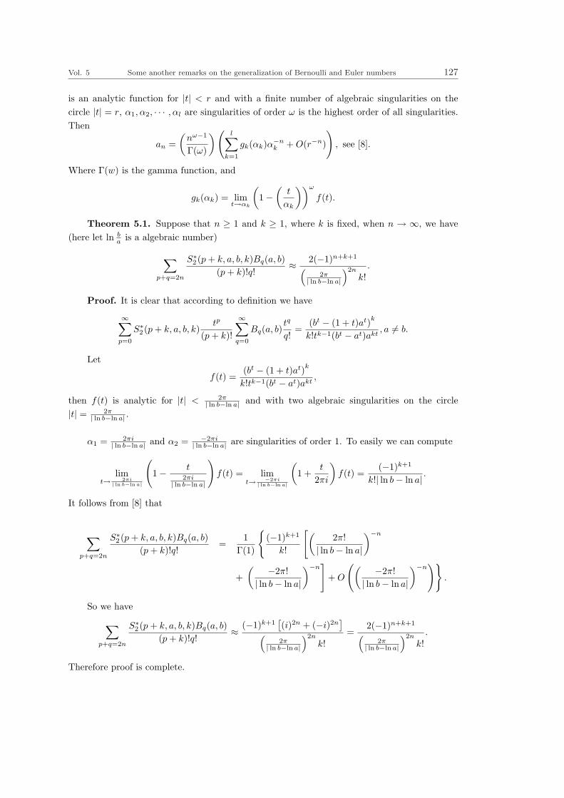
Vol. 5 Some another remarks on the generalization of Bernoulli and Euler numbers 127
is an analytic function for |t| < r and with a finite number of algebraic singularities on thecircle |t| = r, α1, α2, · · · , αl are singularities of order ω is the highest order of all singularities.Then
an =(
nω−1
Γ(ω)
) (l∑
k=1
gk(αk)α−nk + O(r−n)
), see [8].
Where Γ(w) is the gamma function, and
gk(αk) = limt→αk
(1−
(t
αk
))ω
f(t).
Theorem 5.1. Suppose that n ≥ 1 and k ≥ 1, where k is fixed, when n → ∞, we have(here let ln b
a is a algebraic number)
∑p+q=2n
S∗2 (p + k, a, b, k)Bq(a, b)(p + k)!q!
≈ 2(−1)n+k+1
(2π
| ln b−ln a|)2n
k!.
Proof. It is clear that according to definition we have
∞∑p=0
S∗2 (p + k, a, b, k)tp
(p + k)!
∞∑q=0
Bq(a, b)tq
q!=
(bt − (1 + t)at)k
k!tk−1(bt − at)akt, a 6= b.
Let
f(t) =(bt − (1 + t)at)k
k!tk−1(bt − at)akt,
then f(t) is analytic for |t| < 2π| ln b−ln a| and with two algebraic singularities on the circle
|t| = 2π| ln b−ln a| .
α1 = 2πi| ln b−ln a| and α2 = −2πi
| ln b−ln a| are singularities of order 1. To easily we can compute
limt→ 2πi
| ln b−ln a|
(1− t
2πi| ln b−ln a|
)f(t) = lim
t→ −2πi| ln b−ln a|
(1 +
t
2πi
)f(t) =
(−1)k+1
k!| ln b− ln a| .
It follows from [8] that
∑p+q=2n
S∗2 (p + k, a, b, k)Bq(a, b)(p + k)!q!
=1
Γ(1)
(−1)k+1
k!
[(2π!
| ln b− ln a|)−n
+( −2π!| ln b− ln a|
)−n]
+ O
(( −2π!| ln b− ln a|
)−n)
.
So we have
∑p+q=2n
S∗2 (p + k, a, b, k)Bq(a, b)(p + k)!q!
≈ (−1)k+1[(i)2n + (−i)2n
](
2π| ln b−ln a|
)2n
k!=
2(−1)n+k+1
(2π
| ln b−ln a|)2n
k!.
Therefore proof is complete.

128 Hassan Jolany and M. R. Darafsheh No. 3
§6. New method for representation of Apostol Bernoulli
and Euler polynomials
Let σ(n) denote the set of partitions of n (a nonnegative integer) usually denoted by1k12k23k3 · · ·nkn with
∑iki = n
For nonnegative integral vector k = (k1, k2, . . . , kn), the multinomial coefficient(
xk
)as usual,
is defined by(x
k
)=
(x)|k|∏(ki)!
,
where the finite product∏
runs over i from 1 to n, (x)k stands for the all factorial notation,and |k| represents the coordinate sum for the vector k = (k1, k2, . . . , kn). Now let
[g(t)]x =∑
n≥0
An(x)tn,
where x is an arbitrary complex number independent of t.Theorem 6.1.([11]) For arbitrary complex number x and y,
An(xy) =∑
σ(n)
(x
k
) ∏[Ai(y)]ki
So according to these theorems we have the following results.Corollary 6.1. Let α, β are complex numbers then we have the following identities
B(αβ)n = n!
∑
σ(n)
(α
k
) ∏(B
(β)i
i!
)ki
,
E(αβ)n = n!
∑
σ(n)
(α
k
) ∏(E
(β)i
i!
)ki
.
Proof. Let An(α) = B(α)n
n! in theorem 6.1.
References
[1] Qiuming Lue, Euler polynomials of higher order involving the stirling numbers of secondkind. (accepted)
[2] Guodong Liu, Generating functions and generalized Euler numbers Proc. Japan Acad.Ser. A Math. Sci. Volume 84, 2(2008), 29-34.
[3] E. T. Whittaker, G. N. Watson, A Course of Modern Analysis, cambridge universitypress, page 147.
[4] C. Frappier, Representation formulas for entire functions of exponential type and gen-eralized Bernoulli polynomials, J. Austral. Math. Soc. Ser., No. 3, 64(1998), 307-316.
[5] Hugh L. Montgomery, Robert C. Vaughan, Multiplicative number theory I. Classicaltheory, Cambridge tracts in advanced mathematics, 2007, 97.

Vol. 5 Some another remarks on the generalization of Bernoulli and Euler numbers 129
[6] Boyadzhiev, Khristo N. Apostol-Bernoulli functions, Derivative polynomials and Eule-rian polynomials. ArXiv: 0710.1124.
[7] L. Comtet, advanced combinatorics, reidel, 1971 .[8] M. Wachs and D. White, p, q-Stirling numbers and set partition statistics, j.combin.
theory, 56(1990).[9] D. H. Lehmer, lacunary recurrence formulas for the numbers of Bernoulli and Euler,
Annals of Mathematics, 1935, 637-649.[11] S Ramanujan, Some properties of Bernoulli numbers Indian Mathematical Journal,
December, 1911.[11] W. C. Chu and R. k. Raina, Some summation formulate over the set of partitions,
Acta Math. Univ. Comenianae Vol. LXI, 1(1992), 95-100.[12] Hassan Jolany, M. R. Darafsheh, Some relationships between Euler and Bernoulli
polynomials. (submitted)
