scientific report meteoswiss no. 95 quantifying the ... · meteoswiss for both the automatic rain...

Scientific Report MeteoSwiss No. 95

Quantifying the uncertainty of spatial precipitation

analyses with radar-gauge observation ensembles

Raphaela Vogel

MeteoSwiss

Krähbühlstrasse 58

CH-8044 Zürich

T +41 44 256 91 11

www.meteoschweiz.ch

ISSN: 1422-1381


Quantifying the uncertainty of spatial precipitation

analyses with radar-gauge observation ensembles

Raphaela Vogel

Recommended citation:

Vogel, R.: 2013, Quantifying the uncertainty of spatial precipitation analyses with radar-gauge

observation ensembles, Scientific Report MeteoSwiss, 95, 80 pp.

Editor:

Federal Office of Meteorology and Climatology, MeteoSwiss, © 2013

V


Abstract

Sound quantitative precipitation estimates (QPE) are a key component of many hydrological and

meteorological applications. The small-scale variability of precipitation and the limited coverage and

accuracy of observations pose a major challenge to QPE precision. This study investigates a

geostatistical method that combines radar and rain gauge data, to (a) generate best estimate

precipitation fields and to (b) simulate ensembles of random precipitation fields that are consistent

with the observations and represent the inherent analysis uncertainty. Daily precipitation data for

2008 covering the territory of Switzerland are used. Data transformation is applied to improve the

compliance with model assumptions. The accuracy of the point estimates and the reliability of the

probabilistic estimates from kriging with external drift are evaluated. A technical verification and

plausibility experiments comparing the spatial uncertainty of the generated observation ensembles

are performed.

A systematic application for the entire year 2008 shows the combination to improve both the

accuracy of the best estimates and the representation of intense precipitation. Radar information is

particularly beneficial in summer, for distinguishing wet and dry areas, and when the density of the

gauge network is low. Greater improvement in both accuracy and reliability of the QPE can be

achieved, however, with additional gauges from a denser network rather than with the additional

radar information.

The technical implementation of the conditional simulation procedure is verified to be successful.

Illustrative example cases show the ensemble members to represent the spatial variability of

precipitation and to realize extremes beyond the range of the observations. Ensembles with 100

members are found to be sufficient to plausibly reproduce the spatial uncertainties. The increased

density and improved technology of both the automatic rain gauge and radar network in the future

render the combination very attractive for real-time applications. The results of the conditional

simulation experiments bring to light considerable uncertainties regarding the distribution of true

precipitation, especially at small scales. Observation ensembles are a promising way for describing

these uncertainties quantitatively, and there are interesting prospects for using them to propagate

uncertainties into concrete applications.

VI


Contents

Abstract V

1 Introduction 1

2 Data 4

2.1 Precipitation data 4

2.1.1 Rain gauge data 4

2.1.2 Radar data 5

2.2 Studied events 5

3 Methods radar-gauge combination 7

3.1 Geostatistics 7

3.2 Kriging with external drift 8

3.3 Data transformation 9

3.4 Evaluation 9

3.4.1 Cross validation 9

3.4.2 Skill measures 10

3.4.3 Reliability of the probabilistic estimates 11

3.4.4 Reference methods for comparison 11

3.5 Software 12

4 Radar-gauge merging at the daily time scale 13

4.1 Sensitivity analysis of data transformation 13

4.2 Systematic evaluation of KED for daily precipitation 16

4.2.1 Example case 17

4.2.2 Estimated parameters 18

4.2.3 Accuracy of point estimates 19

4.2.4 Reliability of the probabilistic estimate 24

4.2.5 Representation of intense precipitation 27

4.2.6 Annual precipitation distribution 29

5 Methods ensemble simulation 32

5.1 Fundamentals of conditional simulation 32

5.2 Implemented method for conditional simulation from combined radar-gauge

precipitation data 36

5.3 Discussion of characteristics of the generated observation ensembles 37

5.3.1 Technical verification of generated observation ensembles 37

5.3.2 Comparison of spatial uncertainty 37

VII


5.4 Software 38

6 Results from simulated observation ensembles 39

6.1 Technical verification of the ensembles 39

6.2 Precipitation fields from conditional simulation 43

6.3 Experiments for quantifying the uncertainty reduction attributable to different

method settings 48

7 Conclusions 54

Abbreviations 58

References 60

Acknowledgement 63

A Comparison of ensemble and kriging spread 64

B Precipitation fields from conditional simulation 65

1


Quantifying the uncertainty of spatial precipitation analyses with radar-gauge observation ensembles

1 Introduction

1 Introduction

Precise estimates of precipitation fields are very important in many applications such as hydrological

forecasting (e.g., Zappa et al., 2008; Young et al., 2000; Viviroli et al., 2009) or numerical weather

prediction (e.g., Leuenberger and Rossa, 2007). The increased availability of high-resolution

quantitative precipitation estimates (QPE) fosters such applications. Nevertheless, the precision of

the QPE is constrained by the small-scale spatial and temporal variability of precipitation and the

limited coverage and accuracy of observational monitoring systems. In a country with complex

topography like Switzerland, these limiting factors are particularly significant.

Many climatological applications in Switzerland nowadays use precipitation fields generated with an

interpolation of rain gauge measurements. The most important advantage of the rain gauge

measurements is their accuracy in absolute terms. Their spatial representativity, however, is limited.

Should we gather all 440 rain gauges within Switzerland, the total area covered would amount to less

than 10m2. Additional limitations of rain gauge observations are errors induced by wind or snowdrift,

which affect the accuracy depending on the prevalent precipitation situation (e.g., Sevruk, 1985).

In applications with a real-time focus it is more common to use precipitation estimates from radar

observations. MeteoSwiss runs three weather radars providing data of high spatial and temporal

resolution. Unfortunately, the use of empirical relationships to convert the indirect measurement of

hydrometeor backscatter into a precipitation rate, visibility problems, ground clutter and uncertainties

about the vertical profile render the radar information inaccurate. Due to the mountainous topography

of Switzerland, the estimation of precipitation from backscattering measurements is particularly

difficult and requires complicated processing procedures (see e.g. Germann et al., 2006).

One possible way to cope with the presented limitations of precipitation measurements is increasing

the station density and improving the measurement technology. This is currently done by

MeteoSwiss for both the automatic rain gauge and the radar network. In 2013, the SwissMetNet

(SMN) will include 134 automatic stations, compared to less than 80 in 2009 (MeteoSwiss, 2010).

Furthermore, the existing radar network is currently being updated with state-of-the-art dual

polarization technology and the set up of two more radars in the inner alpine regions of the Grisons

and the Valais is planned (MeteoSwiss, 2012).

A complementary approach is to advance methods of data processing to use the information

delivered by the existing networks in a more beneficial way. As outlined in the previous paragraphs,

rain gauge and radar measurements have opposing strengths and weaknesses. The idea of

combining information from the two different measurement platforms is appealing. Both the high

resolution of radar and the accuracy of rain gauge measurements could thereby be exploited.

Merging radar and rain gauge data has been an intense field of research for many years and

2


different combination methods have been suggested. The inclusion of radar information has been

found to improve the skill of the QPE (e.g., Goudenhoofdt and Delobbe, 2009; Erdin, 2009;

Schuurmans et al., 2007). Combination methods are based either on deterministic (e.g., DeGaetano

and Wilks, 2008) or stochastic interpolation concepts, where stochastic methods have the advantage

of delivering a probabilistic estimate (i.e. a best estimate and an uncertainty measure). A popular

class of stochastic combination methods is constructed within the framework of geostatistics.

Goudenhoofdt and Delobbe (2009) find that geostatistical approaches accounting for the spatial

covariance structure of precipitation fields perform best. Widely used geostatistical methods in the

radar-gauge merging context are ordinary kriging of radar errors, kriging with external drift, indicator

kriging and co-kriging (e.g., Erdin, 2009; Haberlandt, 2007; Seo, 1998; Krajewski, 1987; Sideris et al.,

submitted). Although the exact implementation of the kriging technique differs between applications,

kriging with external drift was demonstrated to be particularly flexible and promising when applied

over mid-sized countries where the structure of radar errors is sufficiently homogenous (e.g.,

Goudenhoofdt and Delobbe, 2009; Erdin, 2009; Haberlandt, 2007; Keller, 2012).

MeteoSwiss is interested in an optimal method to estimate high resolution daily precipitation fields in

near real-time. This places high demands on data availability. The automatic SMN network provides

high quality rain gauge data in real-time but, with only about 130 stations, at very limited spatial

density. A method using the SMN network in conjunction with real-time daily aggregates from radar

has the potential to significantly improve the quality of QPE. If successful, such an implementation

could replace existing daily QPE data products based on gauge or radar data only.

This report presents an implementation and extended evaluation of kriging with external drift at the

daily time scale. This work is heavily based on previous developments by Erdin (2009) and Erdin et

al. (2012). KED is used to estimate precipitation with rain gauge data from the SMN station network.

The precision of the point estimates and the reliability of the probabilistic estimates are compared to

single-sensor reference methods. Our most important research question is the following: what is the

benefit of using aggregated radar fields to estimate daily precipitation fields from the SMN station

network with KED? Further, we are interested in the influence of the station density on estimation

quality. To answer the stipulated questions we perform a systematic application for an entire year.

In spite of the significant improvements realized with geostatistical combination methods, the residual

uncertainty in estimated precipitation fields is still large. Kriging provides a best estimate, which is a

smoothed representation of reality (e.g., Ekström et al., 2007; Goovaerts, 1997; Webster and Oliver,

2007). As kriging minimizes the local error variance, small values are typically overestimated and

large values underestimated (Goovaerts, 1997). In other words, if we randomly select 100 values

from a field obtained as best estimate from kriging and fit a variogram to them, the variance would be

much smaller compared to the variance in the original data. A way to represent the inherent

variability in the observations is to generate stochastic ensembles of precipitation fields by

conditional simulation. Each ensemble member generated by conditional simulation corresponds to a

possible realization of the unknown true precipitation field given the available observations and the

spatial covariance structure. All these realizations are equally probable. The QPE from the fields of

best estimates already have an associated variance giving a clue about the probability with which a

critical precipitation amount is realized at a particular location. Yet, this kriging variance does not

3



1 Introduction

indicate the probability that the mean over a specific area exceeds a critical amount. This joint

probability can be evaluated with the simulated ensembles through an averaging of the probabilities

over a specific area (Webster and Oliver, 2007). The spread of this average between the ensemble

members can be interpreted as the uncertainty in the QPE.

There is growing interest in applying conditional simulation to quantify uncertainties in QPE. The

methods applied and data used differ greatly among studies published. Some studies focus on the

spatial covariance structure only (e.g., Frei et al., 2008; Ahrens and Jaun, 2007; Clark and Slater,

2006), while others also account for temporal correlation in the measurements (e.g., Germann et al.,

2009; Ekström et al., 2007). Whilst in most of the previous studies the simulations are conditioned on

rain gauge measurements (e.g., Frei et al., 2008; Ahrens and Jaun, 2007; Ekström et al, 2007; Clark

and Slater, 2006), Germann et al. (2009) simulate precipitation fields based on radar data and use

rain gauge measurements of the past only to quantify the radar error covariance structure. To test

their hydrological performance, observation ensembles can be fed into a hydrological model. This

yields a distribution of response values with a spread representing the sensitivity of runoff to

uncertainty in the input observations (e.g., Germann et al., 2009; Zappa et al., 2008).

To our knowledge, conditional simulation has not been applied in the context of radar and rain gauge

combination. Yet, Rakovec et al. (2012) and Clark and Slater (2006) point out the potential

improvement of adding radar data to gauge based ensembles. The increased use of combined data

products will fuel new applications where an explicit quantification of uncertainty is desirable. The

development of a stochastic observation ensemble technique in a radar-gauge merging context will

foster such applications and may provide interesting insight into the level of uncertainty reduction

attributable to radar. This thesis presents the first results of applying conditional simulation to merged

radar–gauge data and investigates the plausibility of generated observation ensembles. The

comparison with ensembles simulated with a rain gauge only reference method allows to investigate

the specific benefit of the additional radar information.

The thesis pursues two goals, each addressed separately with a methods and results section. First,

systematic evaluation of KED performance on a daily time scale using observations of the SMN

station network and the operational MeteoSwiss radar composite. Second, application of conditional

simulation to merged radar-gauge data and investigation of the uncertainty structure reflected in the

generated observation ensembles. The structure of this thesis is therefore as follows. The

precipitation data used and the events studied are described in chapter 2. The methodological

background of the systematic analysis of KED is provided in chapter 3. The corresponding results

and their discussion follows in chapter 4 and is split into two parts; the sensitivity analysis of data

transformation and the systematic application of KED on the daily time scale. Chapter 5 describes

the fundamentals of conditional simulation and presents the implemented conditional simulation

technique. The results and discussion section of conditional simulation is presented in chapter 6. We

bring back together the narrative on KED and conditional simulation for the conclusions in chapter 7.

4


2 Data

2.1 Precipitation data

Daily aggregated precipitation data from rain gauges and radar over the domain of Switzerland are

used in this study. The daily precipitation amount of both rain gauges and radar corresponds to the

24 hours sum from 06:00 UTC of a specific day to 06:00 UTC of the following day. All data used in

this study is provided by MeteoSwiss.

2.1.1 Rain gauge data

Rain gauges are a widely used device to measure precipitation. A classical gauge consists of a

barrel with 200 cm2 collecting orifice. This study distinguishes two station networks with different

densities, both operated by MeteoSwiss. The station network termed SMN incorporates observations

from the 75 automatically measuring SwissMetNet (SMN) stations with 10 min time resolution

operational in 2008. In addition to the SMN stations, the second station network ALL also includes

the observations from the 366 climatological stations operated manually with daily time resolution.

The distribution of the rain gauges is shown in Figure 1. The stations are evenly distributed over the

whole domain. High-elevation areas, however, are underrepresented especially in the automatic

SMN network. The data undergoes automatic and manual quality control prior to utilization (Scherrer

et al., 2011). Since implausible observations are excluded from the analysis, the station base varies

over time. Rain gauges are fairly accurate in absolute terms (Frei et al., 2008) and the rain gauge

measurements are assumed to represent the correct values of precipitation at their respective

locations.

Figure 1 Radar composite of precipitation on the 16 May 2008 (mm per day). The radar locations at La Dôle, Monte

Lema and Albis are marked in yellow. The circles indicate the locations of the rain gauges used in this study. The black

circles represent the climatological and the red circles the automatic gauges. The station network referred to as ALL

includes both the climatological and the automatic gauges, whereas SMN only includes the automatic SMN gauges.

Radar

Automatic gauge

Climatological gauge

5



2 Data

2.1.2 Radar data

A weather radar is an active remote sensing instrument sending out electromagnetic wave pulses.

The reflectivity of backscattered radiation by hydrometeors, R, is measured and turned into an

estimate of the rain rate Z based on an empirical relationship of the form Z=a*Rb. At MeteoSwiss, the

relation

is used (Germann et al., 2006). In 2008 - the period examined in this study - MeteoSwiss operated

three C-band radars located in Central (Albis), Western (La Dôle) and Southern (Monte Lema)

Switzerland (see Figure 2.1.1). We use composites from the three radars with a grid spacing of 1 km

and a time resolution of one day, inferred by accumulation of 5-minute composites. We refer to

Germann et al. (2006) for a detailed description of radar data processing implemented in

Switzerland. The radar values at gauge locations are determined by nearest neighbor, i.e. by the

radar value of the nearest grid point.

2.2 Studied events

Erdin et al. (2012) performed a systematic evaluation of KED for hourly precipitation over one year.

Since they used the year 2008, this thesis also uses data from 2008 for the systematic application of

KED to daily precipitation sums. This theoretically enables the comparison of estimation quality

between the daily and hourly time scales.

The conditional simulation procedure applied in this thesis is a first exploratory step into a new field.

We perform it as a case study and investigate three different precipitation events on the daily time

scale (see Figure 2). We choose the 8 August 2007 as an example of stratiform precipitation due to

intense precipitation fallen all over Switzerland. In the west, rain gauges and radar observations

show a strong disagreement. The 10 June 2008 is characterized by isolated convective precipitation

with intense fine-scale precipitation cells present. Radar and rain gauge measurements are agreeing

well. Overall convective precipitation was encountered on the 6 September 2008. Precipitation is

abundant all over the domain, with a distinct maximum in the Ticino.

In addition, monthly aggregates from daily precipitation for the three months of January, May and

July 2008 are studied.

6


Figure 2 Radar composite and rain gauge measurements of the three example days investigated in the case study of

conditional simulation. For every example day the characteristic precipitation situation is indicated. The value of the

transformation parameter λ (see section 3.3 for a description of data transformation) is given for the combination (KED

and CSCOMB) and the single-sensor reference (OKGAU and CSGAU) for both station networks. The radar coefficients

β (from equation 1, section 3.2) are provided for the combination with both station networks. More information on the

parameters, the combination and the reference method follow in section 3 and 5. Values are given in mm with the same

scale for every image.

08 August 2007

Stratiform precipitation

Combination (KED/CSCOMB):

βsmn = 0.368, βall = 0.335

λsmn = 0.523, λall = 0.602

Single-sensor reference (OKGAU/CSGAU):

λsmn = 0.62, λall = 0.715

10 June 2008

Isolated convective precipitation


βsmn = 0.938, βall = 0.888

λsmn = 0.26, λall = 0.309


λsmn = 0.266, λall = 0.275

06 September 2008

Overall convective precipitation


βsmn = 0.777, βall = 0.675

λsmn = 0.302, λall = 0.341


λsmn = 0.358, λall = 0.365

7



3 Methods radar-gauge combination


The theoretical background of the systematic evaluation of daily precipitation fields estimated with

KED is provided in this chapter. Section 1 presents the fundamentals of geostatistics. The second

section is dedicated to the specific radar-gauge combination used. The applied data transformation is

discussed in section 3. A detailed description of the evaluation technique is provided in section 4. In

Section 5 follows a specification of the software used.

3.1 Geostatistics

Geostatistics uses spatially referenced data from a continuous varying field to provide estimates of a

variable wherever desired. In the following, the basic principles of geostatistics are discussed. For

more detailed information readers are referred to Cressie (1993), Goovaerts (1997) or Webster and

Oliver (2007).

In geostatistics, precipitation at a certain point in space is interpreted as a realization of a multivariate

random variable. The characteristics of this random variable can be described by a parametric

model. Such a stochastic concept is helpful since information on the deterministic processes causing

the variability of precipitation is limited. The available precipitation observations are perceived as one

realization of this multivariate random variable. The underlying model decomposes the random

process in a deterministic and a stochastic component. The deterministic component (trend)

corresponds to a first approximation of the field and can be a constant value or a linear model similar

to a linear regression. The stochastic component describes the spatial covariance structure of the

deviations from this trend field (the random process).

Modeling the random process necessitates two assumptions. First, we assume the random process

to be of Gaussian distribution in some transformed space (see later). Second, we have to make

stationarity assumptions. Since observations are sparse with regard to the large domain, we assume

the random process to have certain attributes that are the same everywhere. The concept of weak

stationarity is used here. Weak stationarity assumes the expected value and the variance of the

Gaussian distribution to be constant and the covariance to depend only on the lag distance between

two points (rather than on their absolute position).

The random process is modeled with a parametric semivariogram model. Figure 3 shows such a

variogram for the 10 June 2008. It manifests what is intuitively clear: The variance between

observations increases with increasing lag distance. The fit of an exponential variogram function to

the data requires the estimation of the variogram parameters nugget, a measure of spatially

unstructured variation, sill, the variance of the stochastic process and range, the maximum distance

over which observations are correlated.

Kriging is the geostatistical estimation method corresponding to the stochastic model just outlined. By

kriging we can produce a best estimate of precipitation and a measure of its uncertainty (i.e. the

kriging variance) for every location in the domain. The estimates are weighted linear combinations of

the data, with weights determined by the variogram. Kriging is optimal in the sense that it produces

8


unbiased estimates and minimizes the estimation errors. The following section describes the specific

kriging technique applied.

3.2 Kriging with external drift

KED is a popular kriging technique in the radar–gauge merging context (e.g., Erdin et al., 2012;

Haberlandt 2007; Schuurmans, 2007; Goudenhoofdt and Delobbe, 2009). The deterministic

component (i.e. trend or drift) of KED is based on external data. We use radar information for this

external drift. The KED technique used here was implemented by Erdin (2009) and refined by Erdin

et al. (2012).

The precipitation amount P (in some transformed space, see later) on the target grid with indices i

and j and a resolution of 1 km2 is modeled as follows:

(1)

where α and β are the intercept and the radar coefficient of the deterministic part. Radari,j is the radar

value at the given grid point and Z refers to a random process representing the multivariate Gaussian

random variable of the residuals (i.e. the deviation of gauge observations from the trend).

All the model parameters are estimated jointly by maximum likelihood estimation (MLE) for every

studied day. Since it accounts for the limited sample size, we use the method of restricted MLE

(REML) for parameter estimation. An exponential model is used for variogram fitting. As the sample

size for variogram fitting is small, we use an isotropic variogram, i.e. assume the same spatial

Figure 3 Example variogram from KED with the sparse SMN station network for 10 June 2008. The black dots

represent the semivariances of the binned empirical variogram. The dot size and the small numbers above the x-axis

show the number of observed pairs in the specific bins. The fitted exponential variogram function is shown in blue. The

variogram parameters partial sill (dashed black line) is 2.2, the range (red arrow) is 35 km and the nugget (green arrow)

is zero.

Trend; deterministic part

Random process; stochastic part

9




correlation in all the directions. In order to guarantee robust parameter estimation, we only analyze

days with at least ten wet (≥ 0.5 mm per day) SMN stations.

3.3 Data transformation

Precipitation data is non-negative and skewed and therefore deviates from normality. The stochastic

model of geostatistics, however, assumes a Gaussian distribution This violation of model

assumptions can be reduced with appropriate data transformation prior to the application of kriging.

One of the frequently used transformations was proposed by Box and Cox (1964). It has the

following form:

{

( )

with Y* and Y denoting the transformed and untransformed precipitation data. λ serves as the

transformation parameter. KED is performed on the transformed scale and transformation is applied

to both radar and rain gauge observations. The results in transformed space are finally back-

transformed into precipitation space by inverse application of the Box-Cox transformation.

Erdin et al. (2012) studied the influence of data transformation on estimation quality. They find a

case-dependent λ to be the most appropriate choice. We follow this recommendation and estimate

case-dependent λs with MLE for every day and station density specifically. Since excessive

transformation can introduce a positive bias (Erdin et al., 2012), we apply a lower bound to the

estimation of λ with a prior distribution. Section 4.1 provides the results of the sensitivity analysis for

the most appropriate choice of this lower bound. Model diagnostics show that the applied

transformation leads to good compliance with the model assumptions (not shown here).

3.4 Evaluation

In order to assess the performance of KED, we perform an extended evaluation of the quality of the

QPE. Cross validation is the basis for further analysis and explained in the first subsection. The next

subsection presents the skill measures compared. In the third subsection, we present how the cross-

validated probabilistic estimates can be used to investigate the reliability of the probabilistic

estimates, i.e. whether the kriging variance describes uncertainties appropriately. Single-sensor

reference methods used to quantify a potential benefit of the combination are described in subsection

4.

3.4.1 Cross validation

Cross validation is a common technique to assess the skill of spatial interpolation methods and often

applied with radar-gauge combinations (e.g., Haberlandt, 2007; Clark and Slater, 2006). Thereby, the

precipitation amount at a certain gauge location is estimated with a model fitted to the data without

using the measurement at the specific gauge itself. These estimations are then compared to the

observations and the so called cross validation errors are computed from the difference between

observed and estimated values. This procedure is repeated for all the observations successively.

10


We use cross validation at all gauges for precipitation fields estimated with the dense station network

ALL. When using KED with the SMN station network, we perform a test data validation with the

climatological gauges besides the cross validation at SMN stations. The observations at the

climatological gauges were not used for the model estimation and serve as independent set of test

data. The observations at these test locations are compared to the model estimates to yield the

estimation errors from test data validation. For further analysis, cross validation errors and estimation

errors from test data validation are taken together. We have, thus, a complete set of validated

estimates for both station networks. This is important for comparability and guarantees consistency.

3.4.2 Skill measures

The estimation errors from cross and test data validation can be condensed into a variety of skill

measures. Since the different skill measures assess different abilities of a method, it is important not

to rely on one skill measure only, but rather consider a number of different measures. Skill measures

are calculated on a transformed scale to mitigate the predominance of errors at locations with intense

precipitation. We either apply a square root (where not stated differently) or a logarithmic

transformation to both observations and estimations. The transformation can reduce but not remove

the problem that the estimation quality depends critically on the fallen precipitation amounts. Still,

different precipitation situations are hardly comparable. The skill measures used are described

extensively in Erdin (2011) and Keller (2012). A brief description is provided in the following.

The skill measure Bias assesses systematic errors of a method and is computed on logarithmic scale

(in dB). The best measure of the Bias is 0 dB. Negative (positive) values of the Bias refer to an

underestimation (overestimation) of precipitation.

(

∑

∑

)

The relative mean root transformed error (Rel. MRTE) is a measure of overall quality of a method. It

is the MRTE normalized by the mean root transformed deviation (MRTD). For the Rel. MRTE, the

best measure is 0.

(

∑ (√ √ )

∑ (√ √ ̅̅ ̅̅ ̅)

)

Whether a method distinguishes well between wet and dry areas is evaluated with the Hanssen-

Kuipers discriminant (HK). The false alarm ratio (number of wet estimations when observations were

dry, divided by the number of all dry events) is subtracted from the probability of detection (correctly

estimated wet events divided by all the observed wet events) to yield the HK (see Wilks (2006) for

details). Whilst a perfect estimation has a HK of 1, a HK of 0 implies no additional skill of the

estimation over a random estimation.

SCATTER assesses the performance of a method to quantify precipitation in areas where

precipitation is estimated and observed. Proposed by Germann et al. (2006), the skill measure is

defined as half the distance between the 16% and the 84% quantiles of the cumulative error

11




distribution function (CEDF; the cumulative contribution to total precipitation as a function of the

radar-gauge ratio on days where both estimation and observation are wet). A SCATTER of 0 dB

signifies best performance.

( )

The stable equitable error in probability space (SEEPS) is a three category error measure. It

assesses the ability of a method to distinguish between dry, light (defined as the lower two thirds of

all wet observations) and intense (upper third) precipitation. More Information on SEEPS is supplied

in Rodwell et al. (2010). The best measure of the SEEPS is 0.

The median absolute deviation (MAD) is, as the Rel. MRTE, a measure assessing the overall quality

of a method. Yet, it is less influenced by outliers. A MAD of 0 refers to an error-free estimation.

(|√ √ |)

3.4.3 Reliability of the probabilistic estimates

The reliability of the QPE is assessed by comparing the gauge measurements with the probability

density function (pdf) of the corresponding cross-validated probabilistic estimate. For a probabilistic

forecast (i.e. a probabilistic prediction in space), reliability refers to the statistical consistency

between estimated probabilities and observed relative frequencies (Wilks, 2006). In a fully reliable

system, we would expect the frequency of gauge measurements smaller than quantile Qp of its

pertinent cross-validated probabilistic estimate to be p. We can compare the observed frequencies of

measurements to fall into predefined interquantile bins of the probabilistic estimates to the expected

frequencies in a fully reliable system. This provides information on the reliability of the kriging

estimations. This reliability assessment is similar to the Talagrand diagram (Talagrand et al., 1997).

3.4.4 Reference methods for comparison

In this thesis we compare the estimation quality of KED to three single-sensor reference methods.

They help to illustrate and quantify potential improvements achieved by combining radar and rain

gauge data with KED. The reference methods used are ordinary kriging of gauges (OKGAU), a

deterministic spatial interpolation (RHIRES), and a QPE product from radar (RADAR). OKGAU and

RHIRES use information from rain gauges and RADAR uses radar information only.

OKGAU performs an ordinary kriging of gauge measurements. Since ordinary kriging is a

geostatistical kriging technique, OKGAU has a deterministic and a stochastic part comparable to

KED. In contrast to KED, however, the trend field in OKGAU is a constant (i.e. the mean of the gauge

observations). Information on the spatial covariance structure of the deviations of gauge observations

from the mean are added. OKGAU also supplies the kriging variance and allows evaluating the

reliability of the estimates. Transformation, variogram modeling and parameter estimation are

performed as for KED.

12


Data from all the automatic and climatological gauges are used in RHIRES. The analysis consists of

an angular distance weighting scheme in combination with a local regression analysis. Details can be

found in Frei and Schär (1998) and Frei et al. (2006). Here, RHIRES is used as a reference for

comparing aggregated yearly precipitation.

Fields estimated with RADAR correspond to the radar composites also used for KED. We refer to the

data section 2.1.2 and Germann et al. (2006) for a more detailed description of this radar product.

The radar data supplied by MeteoSwiss are on the target grid already and need no further

interpolation.

For ease of understanding, the different methods are designated hereafter in the following way:

KED_all and KED_smn refer to the precipitation field estimated with the radar-gauge combination

method KED and the station networks ALL and SMN. Estimations with OKGAU are called

OKGAU_all and OKGAU_smn respectively. The two other reference methods are simply called

RHIRES and RADAR.

3.5 Software

We use the free statistical software R, version 2.14.0 (R Development Core Team, 2011), for all the

statistical analysis, plots and calculations performed. The geostatistical methods applied are based

on the R-package geoR (Ribieiro and Diggle, 2001).

13



4 Radar-gauge merging at the daily time scale

4 Radar-gauge merging at the daily time

scale

We present and discuss the results of applying KED to estimate daily precipitation in this chapter. As

motivated in the method section, we dedicate a first section to the analysis of the sensitivity of

estimation quality on data transformation. In section 2 we show the results of the systematic

application of KED for the entire year 2008.

4.1 Sensitivity analysis of data transformation

The importance of transformation to precipitation data was pointed out in section 3.1. Yet, Erdin et al.

(2012) show that excessive transformation can result in a positive bias in the QPE. They find that 'as

a consequence of the excessive skewness and precipitation dependence', experiments with

prescribed λs lower than 0.2 resulted in such positive biases. The introduction of a lower bound to

the transformation parameter λ was recommended. The lower bound could be implemented in the

form of a prior distribution that operates as a constraint to the MLE of λ to avoid excessive

transformation. On the hourly time scale, λ=0.2 was suggested as a sensible choice for this lower

bound (Erdin et al., 2012).

Whether this setting of a lower bound of λ (λlower) should be adopted for the daily time scale requires

a careful sensitivity analysis. On the one hand, we want a λlower such that excessive transformation is

prevented. On the other hand, this lower bound should be low enough to allow MLE to find the most

suitable λ for the given data. Hence, we perform cross validation to examine the accuracy of the point

estimates and the reliability of the probabilistic estimates of different λlower.

For this sensitivity analysis, we use a test period of 134 days in the six months of January, May,

June, July, August and September of the year 2008. Considered are days when more than ten

gauges registered precipitation. The fields are estimated with KED_all that serves as illustration

example. We investigate the sensitivity of estimation quality to λlower with two different settings, λlower

fixed at 0.2 and 0.3. The selection is motivated by the fact that λlower =0.2 proved to be the most

successful choice for hourly precipitation. As the skewness of daily precipitation is expected to

Figure 4 Histogram of the estimated transformation parameters λ from MLE for the two settings of λlower (λlower =0.2 and

λlower =0.3). The realized values of λ (x-axis) are plotted against the number of days (y-axis) the specific λs were

estimated. The label on the x-axis indicates the lower bound of the respective bin.

14


breduced compared to hourly precipitation, the λs realized on daily time scales will likely be higher

and probably need a higher lower bound. Thus, we compare the impact of λlower =0.2 on estimation

quality to the one with λlower =0.3.

We first turn towards the realized λs, i.e. the λs that were estimated by MLE given the constraint of

the two different lower bounds (see Figure 4). For both λlower, the majority of estimated λs are close to

the lower bound. The number of λs in the lowest bin increases for λlower =0.3, as it also includes many

of the λs that fell into bins between 0.225 and 0.3 in the case of λlower =0.2. Yet, the λs estimated with

λlower =0.3 tend to be higher also well above the threshold of 0.3. Whilst only on 19 days a λ

exceeding 0.4 is estimated with λlower = 0.2, this figure goes up to 29 for λlower =0.3. We therefore

argue that the choice of λlower really influences the MLE of λ.

Figure 5 shows the estimated fields of precipitation on the 11 May 2008 with the two different settings

of λlower. Indeed, the case is representative for the experience that the best estimates are generally

very similar between the two settings of λlower.

As the estimated fields do not reveal much about the quality of the estimation, we compare the skill

measures of the two settings. The differences in skill between the two λlower for the complete sample

of 134 estimated days are negligible (see Table 1). We do not find a positive bias for λlower =0.2. The

Bias is rather less negative and even smaller in absolute terms compared to λlower =0.3.

Table 1: Skill measures Bias, Rel. MRTE, HK, SCATTER and SEEPS from systematic cross validation of KED_all for

the two settings of λlower (λlower=0.2 and λlower=0.3). Skill measures are calculated from the pooled results of the 134 days

of the test period.

Bias (dB) Rel. MRTE HK SCATTER (dB) SEEPS

0.2 -0.01 0.10 0.84 1.32 0.17

0.3 -0.06 0.10 0.84 1.31 0.17

λlower = 0.2

λlower = 0.3

Figure 5 Best estimate fields of precipitation for the 11 May 2008 with KED_all for the two settings of λlower (λlower =0.2

and λlower =0.3). Realized λs are 0.22 (with λlower= 0.2) and 0.31 (with λlower=0.3). The filled circles represent the rain

gauge measurements.

15




A certain difference in estimation quality between the two settings is evident in the probabilistic

estimates. Figure 6 shows the relative frequencies with which measured precipitation falls into the

predefined interquantile bins of the pertinent cross-validated probabilistic estimates. Frequencies are

expressed relative to a fully reliable system. In a fully reliable system, we would for example expect

25% of the measurements to fall between the 25% and the 50% quantile. Thus, we divide the

observed frequencies by these expected frequencies. A fully reliable system results in a straight line

at 1.

For both λlower, the curves show the typical W-shape also observed for OKGAU and with the sparse

station network (a more detailed discussion follows in section 4.2). Except for the lowest interquantile

bin (below the 0.5% quantile), λlower =0.3 has relative frequencies closer to 1 and is therefore more

reliable in the lower quantiles. In the upper quantiles, however, a lower bound of 0.2 produces more

reliable estimates. In the uppermost interquantile bin (above the 99.5% quantile), the observed

frequency for both λlower is three times higher than the expected. This indicates that very large point

observations are considered as too unlikely by the uncertainty range estimated by KED.

We have another important option to analyze the impact of λlower on the quality of the QPE, namely to

check how well intense precipitation is represented in the estimation of the precipitation fields. Table

2 shows the observed frequencies of measured intense precipitation to fall above the 99.5% quantile

of its pertinent cross-validated probabilistic estimates. In these cases, the probabilistic estimate

considers the observed precipitation as extremely unlikely. The frequency of extreme unlikeliness is

desired to be small. As we look at intense precipitation only, we cannot compare it to the expected

frequency of 0.5% a fully reliable system would exert when considering precipitation of all intensities.

As an example for λlower=0.2, of all 9730 events a rain gauge registered precipitation above 10 mm,

220 (i.e. 2.26%) are classified as extremely unlikely by the pertinent cross-validated probabilistic

estimate.

Overall, the percentage of intense precipitation classified as extremely unlikely by the probabilistic

estimate is lower for λlower =0.2. Especially in the light of the conditional simulations that will be

performed based on KED, a good representation of intense precipitation is important. Thus, λlower=0.2

Figure 6 Frequency of gauge measurements to fall in interquantile bins of the pertinent cross-validated probabilistic

estimate (x-axis). Frequencies are expressed relative to the expected frequency in a perfectly reliable system on log

scale (y-axis). The bins of the distribution are defined by the 0.5%, 2.5%, 5%, 10%, 16%, 25%, 50%, 75%, 84%, 90%,

95%, 97.5%, 99.5% quantiles (dashed vertical lines). Shown are results from KED_all for the 134 days of the test period

with the two settings of the lower bound to lambda, λlower =0.2 and λlower =0.3.

16


has an advantage here. The skill measures (here the Bias, the Rel. MRTE and the MAD; see Table

2) for intense precipitation exceeding predefined thresholds are similar for both settings of λlower.

To summarize, the different λlower do not influence the quality of the best estimates. Yet, some

advantages of λlower =0.2 can be made out when comparing the probabilistic estimates. Coming back

to the dilemma mentioned in the beginning, we see that we do not have the disadvantage of a

positive bias with the lower λlower. Moreover, the advantages of a less constrained MLE and better

representation of intense precipitation clearly favor the choice of 0.2 as λlower. The choice of the lower

bound to λ is therefore 0.2 for our daily application and hence the same as proposed for the hourly

time scale.

This sensitivity analysis was carried out with the geostatistical method of KED using rain gauge

observations from the dense station network ALL. We expect the sensitivity of estimation quality to

data transformation not to be influenced by the number of stations used. Figure 8 of the following

section shows a histogram of the realized λs of KED and OKGAU. No major differences between the

two can be made out. We therefore stick to the choice of λlower =0.2 also for OKGAU and in

applications with the SMN network.

Table 2: Percentage of measured intense precipitation events classified as extremely unlikely (corresponding to the

exceedance of the 99.5% quantile) by the pertinent cross validated probabilistic estimate for the two settings of λlower

(λlower=0.2 and λlower=0.3). Intense precipitation refers to the exceedance of the predefined thresholds of 10, 20, 40 and

80 mm. The number of events where measurements exceeded these thresholds is listed. The skill measures Bias, Rel.

MRTE and MAD are shown for precipitation exceeding the above thresholds. Error measures and percentages are

calculated from KED_all for the 134 days of the test period.

Threshold No. of

events

Observed frequency in

the 99.5% quantile Bias (dB) Rel. MRTE MAD

0.2 0.3 0.2 0.3 0.2 0.3 0.2 0.3 10 mm 9730 2.26% 2.83% -0.32 -0.36 0.37 0.37 3.34 3.34

20 mm 4252 2.99% 3.60% -0.42 -0.44 0.54 0.54 4.73 4.73

40 mm 1032 4.94% 5.14% -0.50 -0.51 0.74 0.74 6.70 6.70

80 mm 104 10.58% 12.50% -0.70 -0.69 1.08 1.04 18.63 18.78

4.2 Systematic evaluation of KED for daily precipitation

Equipped with a carefully chosen λlower, we now turn towards the systematic evaluation of KED. The

systematic analysis of the year 2008 encompasses 218 day where both station densities (SMN and

ALL) registered at least ten wet (≥ 0.5 mm per day) gauges. This constraint is set to avoid robustness

problems in case of very few wet gauges.

In the following we first have a look at the QPE of an example day. Subsection 2 then discusses the

estimated model parameters. The accuracy of the point estimates is investigated in subsection 3. A

fourth subsection is dedicated to analyzing the reliability of the probabilistic estimates. Intense

precipitation is treated in the following subsection 5. The last subsection focuses on the annual

distribution of precipitation.

17




4.2.1 Example case

Before we start discussing the systematic application of KED for the year 2008, let us have a

qualitative look at the precipitation distribution of a single day. The estimated precipitation fields from

KED and the single-sensor references for both station densities are shown in Figure 7 for the 10

June 2008. This example case is characteristic for an intense convective isolated precipitation

situation with several isolated, small-scale and slow moving precipitation cells (see also Figure 2).

The filled circles in Figure 7 show the rain gauge observations. If the field is estimated with SMN

stations only, the SMN stations are framed with red. As they allow for an interesting comparison of

the best estimates with the gauge observations, the climatological stations are still plotted.

RADAR

OKGAU_smn

OKGAU_all

KED_smn

KED_all

Figure 7 Estimated fields of precipitation (in mm) for the 10 June 2008 with RADAR, OKGAU_smn, OKGAU_all,

KED_smn and KED_all. The filled circles represent the rain gauge measurements. For OKGAU_smn and KED_smn,

the SMN stations are highlighted in red.

18


In the RADAR field, precipitation is clearly overestimated. This is particularly visible close to rain

gauge locations, where the RADAR field often deviates from the gauge measurements. We

understand these deviations as the low accuracy of radar information when it comes to point

estimation. The fine-scale precipitation patterns, however, are well represented in the RADAR field.

Also for this day with presumably high spatial variability of precipitation (as manifested in the RADAR

field), precipitation fields from OKGAU are very smooth. Although OKGAU is able to represent the

overall features of the precipitation distribution, the loss of information about the unknown true field is

potentially big. The low skill of the estimation is particularly evident for OKGAU_smn. The estimated

field does not match the observations at climatological gauges at all. Information on the fine-scale

precipitation pattern is clearly lacking.

In the combined QPE, we find a good representation of the fine-scale precipitation pattern. The high

radar coefficients (βKED_all= 0.89, βKED_smn = 0.94; see Figure 2) indicate, after correction of the

systematic overestimation, a lot of agreement between radar and gauge observations. Intense

precipitation observed by the radar is therefore well-represented also in regions between the rain

gauges, and the systematic bias of the radar information is corrected. When radar information is

included, the smaller station network does not seem to lower the quality of the estimated field too

much. The estimated field of KED_smn at climatological gauges (i.e. gauges that were not used to

estimate the model with) compare well with the observations.

This example case suggests that adding radar information to rain gauge measurements is

particularly beneficial in convective situations with high spatial variability of precipitation. This

hypothesis will be supported in the following systematic analysis.

4.2.2 Estimated parameters

Figure 8 Histogram of the estimated transformation parameters λ with OKGAU_smn, OKGAU_all, KED_smn and

KED_all for the 218 estimated days of 2008. The realized values of λ (x-axis) are plotted against the number of days (y-

axis) the specific λs were estimated. The label on the x-axis indicates the lower bound of the respective bin.

19




The transformation parameters λ estimated with MLE are shown in Figure 8 for KED and OKGAU

with both station densities. On 60 to 80 days, the λs fall close to the lower bound of 0.2. All methods

show a similar distribution of the frequencies of realized λs. For KED_smn, however, higher values of

λ are more frequently realized.

Figure 9 compares the radar trend coefficient β (from equation (1)) estimated by KED with both

station densities. The correlation between the two estimates is positive, i.e. the estimates are jointly

adjusted with respect to the agreement of radar and gauge observations at gauge locations. The βs

estimated with KED_smn, however, are systematically larger (i.e. off the 1:1 line). The mean values

of the βs (βmean,KED_all =0.43, βmean, KED_smn =0.59) differ by 0.16. A Student's t-test of this difference is

highly significant with a p-value smaller than 2.2x10-16

. Hence, KED_smn has significantly more trust

in the radar information. This could be due to the fact that climatological stations are often located in

complex terrain where radar is more uncertain. As KED_all includes these stations in model

estimation, we expect the radar-gauge relation to suffer from the larger errors and the βs to be

smaller.

4.2.3 Accuracy of point estimates

To assess the accuracy of the point estimates from cross and test data validation, we compare the

skill measures of KED to the skill measures of the single-sensor references (OKGAU and RADAR)

for the sparse and the dense gauge network. In Table 3, the skill measures are shown for the entire

year 2008.

The ranking of the different settings is surprisingly constant among all measures. KED_all always

shows most skill, followed by OKGAU_all, KED_smn and OKGAU_smn. Estimating precipitation with

RADAR has least skill.

This is most evident considering the Bias. The systematic error of the RADAR is much higher than

the error of the geostatistical interpolation method with least skill (OKGAU_smn). Differences

between KED and OKGAU with the same number of stations are marginal. They both have a small

Bias when the sparse network is used. Adding the climatological gauges renders the estimation

Figure 9 Scatterplot of the estimated radar coefficients β for the two methods KED_all (x-axis) and KED_smn (y-axis).

Each dot represents one of the 218 days included in the systematic analysis for the year 2008. The red line shows the

location where the βs of both station densities are equal.

βKED_all

βK

ED

_s

mn

20


virtually bias-free. An interpretation for this might be the higher relative abundance of climatological

gauges located in complex terrain. Neighboring climatological gauges possibly detect precipitation

invisible for the radar and missed by the SMN network. Information about this precipitation remains in

the model, also if one of the gauges observing it is excluded from model estimation by cross

validation. As we will see later on in this section, the Bias can be distorted by compensating positive

and negative deviations. We should therefore interpret these results with care.

The Rel. MRTE, a measure of overall quality of estimation, is reduced to a third from RADAR to

KED_all. The improvement of KED compared to OKGAU, i.e. the benefit of adding radar information,

is more than twice as high when using only SMN stations for model estimation. This does not come

as a surprise. We suggest that the additional information provided by the radar is more urgently

needed in a low density station network.

Table 3: Skill measures Bias, Rel. MRTE, HK, SCATTER and SEEPS from systematic cross and test data validation for

KED and the single-sensor references (OKGAU and RADAR) with the sparse and the dense gauge network. Skill

measures are calculated from the pooled results of the 218 wet days of the year 2008.

Bias (dB) Rel. MRTE HK SCATTER (dB) SEEPS

RADAR -0.43 0.37 0.60 2.89 0.41

OKGAU_smn -0.21 0.21 0.68 1.94 0.31

OKGAU_all 0.06 0.14 0.76 1.49 0.23

KED_smn -0.20 0.17 0.72 1.74 0.27

KED_all 0.02 0.13 0.78 1.37 0.21

Also for HK, SCATTER and SEEPS, the benefit of adding radar information is higher for the SMN

network. Adding information from the climatological gauges, yet, improves the skill measures more

strongly than adding radar information. The HK shows a relatively good ability of RADAR to

distinguish wet and dry areas. This ability is confirmed by the SEEPS, a categorical measure like HK,

showing smaller relative differences between RADAR, KED and OKGAU than the Bias or the Rel.

MRTE.

If the skill measures are calculated for the four seasons individually (Figure 10), interesting details

become apparent. Yet, the ranking of the different methods for all the measures and seasons stays

the same. Whilst the geostatistical methods show a fairly stable Bias for all the seasons, the

systematic errors of RADAR differ a lot. RADAR strongly underestimates precipitation in autumn. In

summer, the Bias of RADAR relative to OKGAU_smn and KED_smn is small. Here, the

compensating effects in the yearly Bias become apparent.

The Rel. MRTE is lowest in autumn and highest in winter for KED and the single-sensor references.

KED_smn is particularly skillful and over-performing OKGAU_all in summer. The added value of

radar is, hence, particularly pronounced in summer and does exceed that from a dense network.

The strongest variation in the HK for the different seasons is found for RADAR. With RADAR, the

distinction between wet and dry areas is best in autumn, i.e. the season where it has the highest

systematic errors. The geostatistical kriging methods perform similar in all seasons. Again, KED_smn

is equally skillful as OKGAU_all in summer.

21




This seasonal analysis suggests that radar information is particularly beneficial in summer. We

observe that the relative differences between RADAR and OKGAU_smn, and KED_smn and

OKGAU_all are particularly low in summer. In our view, this must be related to the higher abundance

of convective precipitation. We understand the strength of radar in convective situations as follows.

First, radar provides beneficial information on the fine-scale structure of local convective precipitation

cells due to its high spatial resolution. The dense network alone cannot compensate the lack of fine-

scale information, because its spacing is still coarse in relation to the typical scale of patterns in

summer. Second, convective precipitation is formed in higher altitudes in summer and therefore has

better radar visibility. In the three other seasons, however, the added value of the climatological

gauges outperforms the additional radar information. The skill of KED_smn is lower than the skill of

OKGAU_all. A reason for this is the rather small-scale structure of radar errors (from shadowing by

mountains) that is difficult to represent in the trend component of KED. The effective resolution of the

precipitation patterns with the dense station network is therefore higher than with the radar.

Bias

Rel. MRTE

HK

Figure 10 Skill measures Bias (in dB), Rel. MRTE and HK from systematic cross and test data validation for KED and

the single-sensor references (OKGAU and RADAR) with the sparse and the dense gauge network. The 218 estimated

days are split into the four seasons.

22


Figure 11 shows the skill measures for four different regions of Switzerland, namely the Swiss

Plateau, the Jura, the Alps and the South. The Bias shows the most complex regional fluctuations of

all the analyzed skill measures. These regional fluctuations are stronger for RADAR than for KED

and OKGAU. Focusing on the geostatistical interpolation methods, we see that the regional

differences with the sparse station network are bigger than with the dense network. The Bias is

generally lower when the dense station network is used. Yet, OKGAU_smn and KED_smn have a

lower Bias in the Swiss Plateau compared to OKGAU_all and KED_all. Except for the Jura, KED

tends to have a lower Bias than OKGAU.

The differences between the regions are surprising. Whilst KED and the single-sensor references all

have negative Biases in the Jura and the South, the opposite happens in the Swiss Plateau. The

Alps are the only region where the Bias of the different methods reflect the pattern seen in the Bias

for all Switzerland. The particularly low alpine Bias of KED_all and OKGAU_all support the

aforementioned hypothesis of the beneficial higher abundance of climatological gauges in complex

terrain. The regions with positive and negative Bias partly compensate such that the overall Bias is

Bias

Rel. MRTE

HK

Figure 11 Skill measures Bias (in dB), Rel. MRTE and HK from systematic cross and test data validation for KED and

the single-sensor references (OKGAU and RADAR) with the sparse and the dense gauge network. Measures are

calculated on the 218 estimated days of 2008 for the four regions Swiss Plateau, Jura, Alps and South individually.

23




reduced. More specifically, the positive Bias in the Swiss Plateau is to some degree compensated by

the negative Biases in the South and the Jura. The highest absolute compensation is thereby

realized for RADAR.

The Rel. MRTE of the geostatistical interpolation methods is, compared to RADAR, low in all regions.

Using gauge observations strongly reduce the Rel. MRTE. The combination achieves a further

reduction of the estimation errors. The Rel. MRTE is particularly high in the Alps and the Jura. We

suggest this to be caused by the reduced radar visibility and a certain underrepresentation of rain

gauges in these high-elevation areas.

RADAR

OKGAU_smn

OKGAU_all

KED_smn

KED_all

Figure 12 Values of the skill measure Bias (in dB) at all stations individually for KED and the single-sensor references

(OKGAU and RADAR) with the sparse and the dense gauge network. Results are shown for the 218 estimated days of

the year 2008.

24


The HK is fairly similar in all regions, i.e. the distinction between wet and dry areas is not so much

influenced by regional characteristics. In the Jura the HK of RADAR is particularly low. We interpret

this as being caused by radar visibility issues, too. The systematic underestimation of precipitation

(i.e. the negative Bias) and the high Rel. MRTE of RADAR in the Jura support this hypothesis. In the

HK this can result to some extent in days with wet observations being misclassified as dry days. The

inclusion of gauge information increases the HK in all regions. Although OKGAU does not include

information on the fine-scale precipitation pattern from radar, the distinction between wet and dry

areas has more skill compared to RADAR. The addition of radar information in the combination leads

to higher values of the HK in all regions. Still, OKGAU_all outperforms KED_smn and has a HK only

slightly smaller than KED_all.

To further highlight how different effects compensate each other in the calculation of the Bias, we

zoom into the regions and look at the distribution of the Bias at all station locations. The most

remarkable pattern of the Bias (Figure 12) is found for RADAR. There is a strong geographical

pattern in the sign of the bias: cross-validated estimations at stations in the South, the Alps and the

Jura underestimate precipitation. This underestimation is particularly strong in the Grisons and the

Valais. We argue that this underestimation is caused by radar visibility problems in mountainous

regions. Contrarily, precipitation is overestimated in northern Switzerland around the Albis radar.

There are, however, a few stations in the eastern and western Swiss Plateau region where

precipitation is underestimated; most likely, again, due to shadowing by mountains. These stations

with negative Bias compensate the overall positive Bias in the region of the Swiss Plateau. The

comparatively low positive Bias in the Swiss Plateau (see Figure 11) is, hence, a result of

compensatory effects.

None of the geostatistical interpolation methods show this clear a pattern. Positive and negative

Biases are distributed more evenly across Switzerland. As the strong north-south gradient of the Bias

is not visible with KED, we suggest that the radar-gauge combination is suitable to mitigate the

systematic Bias of the radar information. The differences between KED and OKGAU are generally

small. Table 3 showed a negative Bias when the sparse and a weak positive Bias when the dense

station network is used. This is reflected in Figure 12. With KED_smn and OKGAU_smn, positive

Biases seem to be more abundant. Yet, as the negative Biases are stronger in magnitude, they

compensate the more numerous but smaller positive Biases. With the dense station network, the

Biases seem systematically lower. Compared to KED_smn and OKGAU_smn, the magnitude of the

Bias in mountainous regions (especially in the Jura) is lower. Again, we argue this to be related to the

higher relative abundance of climatological gauges in complex terrain.

In our view, these plots highlight the partial compensation of positive and negative Biases at

individual stations in the overall Bias. The effective compensation might be even larger, since the

yearly Bias at one station to some degree includes compensating positive and negative Biases of

seasonal precipitation, too.

4.2.4 Reliability of the probabilistic estimate

In this section, we turn away from the point estimates and move towards the probabilistic estimates.

As Figure 6 of the previous section, Figure 13 shows the relative frequencies with which measured

precipitation falls into the predefined interquantile bins of the pertinent cross-validated probabilistic

25




estimates. The analysis of the probabilistic estimates is only possible for the geostatistical

interpolation methods, as the quantiles are calculated based on the inherent kriging variance. The

assessment of the reliability of the probabilistic estimates validates whether this kriging variance

describes the uncertainties appropriately. This provides information on how well the simulated

observation ensembles discussed in chapter 6 represent the degree of uncertainty inherent in the

model.

Both KED and OKGAU produce W-shaped curves. Measurements fall too often below the 0.5% and

above the 99.5% quantile. This means that the probabilistic estimates underestimate the true

uncertainty in general. The overconfidence in the 0.5% quantile is mainly due to dry stations falling

beyond the narrow pdfs when precipitation is weak. This does not raise serious concerns. The

apparently strong overconfidence above the 99.5% quantile is caused by only a small part of the

observations. Compared to the application of KED with untransformed precipitation data, the

reliability is strongly improved (Erdin et al., 2012). Furthermore, measurements fall slightly too often

in mid quantile bins and too seldom into moderate lower and upper quantile bins.

The reliability of the probabilistic estimates does not crucially depend on the station density. Still, the

geostatistical methods using the same station density are more similar than the ones using the same

interpolation technique. Except for the lowest and highest quantiles, the methods using the SMN

stations only perform slightly better, i.e. have relative frequencies closer to 1.

The seasonal probabilistic estimates for summer and winter are shown in Figure 14. Looking at the

seasons individually confirms the findings drawn for the whole year. There are no extreme deviations

apparent. In summer, however, relative frequencies do not go beyond three, whereas they get close

to four in winter. For the quantiles above the median, the station density influences the reliability in all

seasons.


estimate (x-axis). Frequencies are expressed relative to the expected frequency in a perfectly reliable system on log

scale (y-axis). The bins of the distribution are defined by the 0.5%, 2.5%, 5%, 10%, 16%, 25%, 50%, 75%, 84%, 90%,

95%, 97.5%, 99.5% quantiles (dashed vertical lines). Shown are the results from the systematic application over the

year 2008 (218 days) for the comparison of the methods OKGAU_smn, OKGAU_all, KED_smn and KED_all.

26


The differences in the probabilistic estimates among the four dedicated regions are much bigger than

the seasonal differences. The reliabilities of the different regions differ in both magnitude and shape.

Still, all regions show a kind of W-shape for all the methods. In the South (see Figure 14), the

frequency of estimates to fall into the lowest and highest quantile is larger than in the other regions

(i.e. stronger overconfidence). This strong overconfidence is seen for OKGAU and KED with both

network densities. In the Jura region, the overconfidence is reduced. The reduction is particularly

pronounced if ALL gauge observations are used. Whilst the additional radar information does not

increase the reliability of the QPE, the increase in reliability due to the climatological gauges is

considerable. Estimations in the Alps show most reliability (not shown).

Not only the quality of the point estimates but also the reliability of the probabilistic estimates is

considerably influenced by regional differences. Can we deduce from this that a stationarity

assumption for the whole domain of Switzerland is problematic? The assumption of weak stationarity

is certainly a simplification. The reason for the particularly strong overconfidence in the South could

lie in the generally more intense precipitation and higher spatial variability compared to the other

regions. The estimated variogram for all Switzerland is therefore less representative in the South. As

an example, the sill tends to be too small and hence, the pdf of the probabilistic estimate too narrow.

Robust regional variogram estimation is, due to the limited data, technically unfeasible and would

render the conditional simulation of spatially consistent precipitation fields impossible. Furthermore, a

solution at the borders of the regions would have to be found such that the coherence of the

estimated precipitation fields is guaranteed.

Summer

Winter

Jura

South


estimate for the seasons summer and winter (top), and the regions Jura and South (bottom). Legend and axes as in

Figure 13. Note that the scale changes from seasonal to regional plots.

27




Table 4: Percentage of measured intense precipitation events exceeding predefined thresholds classified as extremely

unlikely (corresponding to the exceeding of the 99.5% quantile) by the pertinent cross-validated probabilistic estimate for

OKGAU_smn, OKGAU_all, KED_smn and KED_all. The number of events where measurements exceeded the

thresholds and their percentage with respect to all measurements (climatological frequency) are listed.

Threshold

No. of

events

Climatological

Frequency

Observed frequency in 99.5% quantile

OKGAU_smn OKGAU_all KED_smn KED_all

10 mm 17926 11.41% 3.40% 2.46% 3.36% 2.30%

20 mm 7269 4.63% 5.10% 3.70% 4.60% 4.60%

40 mm 1583 1.00% 8.40% 6.50% 6.80% 6.30%

80 mm 138 0.10% 19.60% 13.80% 10.10% 13.80%

Overall, we see that the probabilistic estimates for the entire year over the whole domain smooth out

some regional and seasonal deviations. Yet, we do not interpret these seasonal and regional

differences as showing major limitations of our method and carry out no further investigations on the

issue.

4.2.5 Representation of intense precipitation

Since it is the intense precipitation that causes most damage and harm, its representation is of

particular interest in many applications. How well intense precipitation is represented in the QPE is

investigated here. We continue the evaluation of the probabilistic estimates specifically for intense

precipitation events where measurements exceeded 10, 20, 40 and 80 mm on a single day.

As in Table 2, Table 4 shows the observed frequencies of measured precipitation to be above the

99.5% quantile of its pertinent cross-validated probabilistic estimates. As expected, the fraction of

intense precipitation classified as extremely unlikely increases for KED and OKGAU with both station

densities for increasing thresholds. As mentioned in section 4.1, restricting the scope to intense

precipitation only does not allow the comparison of the observed frequencies above the 99.5%

quantile with the expected frequency of 0.5% a fully reliable system would exert when considering

precipitation of all intensities. For this reason, we do not know what an appropriate frequency of

'extreme unlikeliness' should be. It is, however, desirable that this frequency stays reasonably small

so that a user exploiting the probabilistic estimates can still be confident that the pdfs consider

extreme events as possible when they occur.

In general, intense precipitation is well represented by the probabilistic estimate of both KED and

OKGAU. As an example, only 14 of the 138 times a rain gauge measured precipitation over 80 mm

are considered as extremely unlikely by the probabilistic estimate of KED_smn. The ability of

KED_smn to represent intense precipitation is a beneficial prerequisite for the conditional simulation

to be performed in the next chapter. There are only marginal differences between KED and OKGAU

concerning the representation of intense precipitation. We understand this from the similar reliabilities

(Figure 12) of KED and OKGAU. Nevertheless, for the very intense precipitation of over 40 mm,

additional radar information seems to reduce the overconfidence.

Figure 15 shows the fraction of observed intense precipitation events exceeding 10 mm classified as

extremely unlikely (i.e. the percentage of cases when the measured intense precipitation event falls

28


above the 99.5% quantile of its pertinent cross-validated probabilistic estimate, as before) for all

stations individually. It can easily be seen that the methods relying on the SMN stations classify

precipitation over 10 mm as extremely unlikely more often. We can interpret this, again, with the

stronger overconfidence of KED and OKGAU with the sparse station network. Stations with high

frequencies of missed intense precipitation are spread all over the domain. The regionally different

reliabilities made out in Figure 14 therefore do not manifest when looking at each station separately.

Not only are we interested in the reliability of the probabilistic estimates of intense precipitation, but

also in the accuracy of the point estimates. Figure 16 shows the Bias and the MAD for intense

precipitation exceeding the thresholds of 10, 20, 40 and 80 mm.

For both skill measures, estimation skills for KED and the single-sensor reference methods RADAR

and OKGAU for both station densities decrease as precipitation intensifies. The relative decrease in

skill with intensifying precipitation is most extreme for RADAR and OKGAU_smn. How can we

interpret this decrease in the quality of the point estimates with intensifying precipitation? We argue

that intense precipitation is often particularly localized and cannot be detected extensively by the rain

gauges. Any system of spatial analysis is therefore particularly challenged by intense precipitation.

Also from the skewness of precipitation data, differences between observed and estimated

precipitation tend to be inflated for increased precipitation intensity.

OKGAU_smn

OKGAU_all

KED_smn

KED_all

Figure 15 Fraction of measured intense precipitation events over 10 mm considered as extremely unlikely by the

probabilistic estimates for OKGAU_smn, OKGAU_all, KED_smn and KED_all. Results are given for each station

individually. Extremely unlikely refers to measurements falling into the 99.5% quantile of the pertinent cross-validated

probabilistic estimates.

29




Both the Bias and the MAD can be strongly reduced in the combination. Also concerning the

accuracy of the point estimates of intense precipitation, the added value of the climatological gauges

is higher than the added value of the radar information. The QPE therefore tend to underestimate

intense precipitation in all the considered settings. Again, we understand this as related to the

smoothing inherent to any spatial analysis building on 'best estimate' principles, and to the locality of

the intense precipitation events. This does not explain the underestimation present in the RADAR

estimates, however. One reason for this are the difference in spatial representativity between radar

(areal) and gauge (point) observations. These differences are particularly relevant for intense

precipitation. The present comparison may therefore be of limited significance.

For the very intense precipitation exceeding 80 mm, the inclusion of radar information in the

combination methods is particularly valuable. This strongly increases the skill of the combination with

respect to both the MAD and the Bias. Nevertheless, the dense station network leads to a

considerable additional improvement also in the combination.

4.2.6 Annual precipitation distribution

The aggregated precipitation fields for the entire year 2008 are shown in Figure 17 for RADAR,

KED_all, KED_smn and RHIRES. The idea is to compare the annual precipitation distribution of the

radar-gauge combinations with RADAR and a deterministic interpolation method exploiting all rain

gauge observations and information from topography called RHIRES (we refer to section 3.4.4 for a

description of the methodology).

In the yearly aggregation, the challenges to infer precipitation from radar in high-mountain regions

and in topographically shielded sections are clearly visible. Especially in the Valais and the Grisons

(i.e. the regions where radar information is most erroneous), estimates by RADAR are systematically

smaller than by the gauge-based analyses. On the other hand, RADAR seems to overestimate

Bias

MAD

Figure 16 The skill measures Bias and MAD of systematic cross and test data validation with RADAR, OKGAU_smn,

OKGAU_all, KED_smn and KED_all. Results for intense precipitation with thresholds of 10, 20, 40 and 80 mm.

30


precipitation in Central Switzerland. There are obvious radar artifacts visible pointing away radially

from the Albis radar. These so called radar stripes manifest important visibility problems of the radars

that are hard to correct for.

The annual precipitation distribution estimated by KED_smn shows an important improvement over

RADAR. Especially in regions where radar estimates are systematically biased, i.e. the Grisons and

the Valais, the benefit of the gauge information is evident. The positive precipitation anomaly around

the Albis radar in central Switzerland as manifested in the RADAR is not represented here. The radar

artifacts are reduced but not entirely removed.

The inclusion of the climatological rain gauges yields further improvements of estimated annual

precipitation sums. KED_all produces the smoothest distribution of all methods shown in Figure 17.

The radar stripes are hardly visible and estimation in the Grisons and the Valais seem to be more

realistic.

The precipitation distribution estimated by RHIRES is the most trustworthy. Especially in the Grisons

and the Valais, topographic features are represented more adequately. Yet, the very intense

precipitation exceeding 3000 mm in the Jungfrau region has to be considered with care. RHIRES

relies on measurements with high uncertainty in this region.

RADAR

KED_smn

KED_all

RHIRES

Figure 17 Estimated fields of yearly precipitation in 2008 (in mm) with RADAR, KED_smn, KED_all and RHIRES.

31




Since the annual precipitation distribution estimated with RHIRES is most trustworthy, we compare it

to KED and RADAR. The differences are shown in Figure 18, where red (blue) stands for areas

where RADAR and KED estimate lower (higher) precipitation than RHIRES.

The field differences of RADAR show a strong north-south gradient. In Southern Switzerland

(including the Jura), RADAR strongly underestimates the annual precipitation sum compared to

RHIRES. In the north, it is reverse and annual precipitation is strongly overestimated by RADAR.

This north-south difference in radar bias was already highlighted in Figure 12 and is also found in

other studies (e.g., Keller, 2012). Furthermore, the radar stripes are clearly visible.

If the SMN stations are added and the precipitation fields are estimated with KED, this north-south

gradient is reduced considerably. Positive and negative differences have a more spotty distribution

and absolute differences from RHIRES are reduced. Still, there is a tendency to underestimate

precipitation in the Valais and the Grisons. Although fairly hidden, the radar stripes are still visible. A

strange pattern can be seen in the eastern most part of the Ticino tip, where strong over- and

underestimation are next to each other. We expect this to be related to a beam blocking pattern of

the Monte Lema radar, possibly enhanced by accidental contrasts in rain gauge measurements

between the Southern Grisons and Central Ticino.

Absolute differences and their spatial correlation can be further reduced when the climatological

stations are included (KED_all). Although less pronounced, issues pointed out for KED_smn remain

problematic in mountainous regions.

RADAR

KED_smn

KED_all

Figure 18 Differences in the estimated fields of yearly precipitation in 2008 (in mm) of RADAR, KED_smn and KED_all

compared to the estimated field of RHIRES.

32


5 Methods ensemble simulation

Conditional simulation refers to the stochastic simulation of random variables with prescribed

expected value, spatial covariance structure and the condition that the random variable takes the

value of the observation at observation locations. The conditional simulation technique implemented

here has the same underlying geostatistical model as KED. The theoretical background thus remains

the same and we refer to section 3.1 for the basics of geostatistics. The data for conditional

simulation needs to be of Gaussian distribution too. We therefore perform the simulation in the

transformed space (see section 3.3 for details on the transformation applied to the data). The

precipitation fields are finally obtained by back-transformation.

The chapter is structured as follows. In a first section, the fundamental concept of conditional

simulation is illustrated with basic simulation examples. Then we explain how conditional simulation

is implemented in this study. A third section discusses how the technical verification of generated

observation ensembles is performed and how the degree of uncertainty reduction attributable to

different model specifications is computed.

5.1 Fundamentals of conditional simulation

We perform the conditional simulation on the same grid as KED with precipitation simulated on

370x240 grid points. The covariance matrix used to simulate from is so high dimensional that it is

difficult to explain the fundamental principle of conditional simulation based on it. We therefore make

use of two simple examples here. A more thorough theoretical background can be found in

Lantuéjoul (2002), Wilks (2006) and Webster and Oliver (2007).

Figure 19 Example simulation of Gaussian distributed two-dimensional random vectors with a predefined correlation

and a mean value of (0 0)T. a) Eigenvectors of the covariance matrix in correlated (green) and uncorrelated (red) space.

The covariance matrices correspond to the respective eigenvectors. The dots in b) represent the Gaussian distributed

two-dimensional random vectors x'. A sample of 500 random vectors was simulated. The example is shown in the

transformed space (i.e. the eigenspace; the coordinate axes correspond to the alternative orthonormal coordinate

system represented by the eigenvectors (Wilks, 2006)).

Σ = (

) Σ ’ (

)

e1

e1’ e2

e2’

33




First, we draw two-dimensional random vectors with normally distributed components that have a

predefined correlation (i.e. they are mutually dependent). The conditions of this simulation are fully

specified by a vector (2D) of mean values and a covariance matrix (2x2). We refer to Figure 19 for an

illustration with a numerical example. The diagonal elements of such a covariance matrix Σ are the

variances of the random vector components (S1 and S2). As a measure of joint dispersion, the off-

diagonal elements are the covariance between the values in both dimensions (C1,2).

Σ (

) (2)

Unless these off-diagonal elements are zero, the values are correlated.

It is most convenient to perform the simulation in a transformed coordinate system, where the two

(transformed) vector components are uncorrelated. This permits the application of conventional

univariate random number generators, sequentially for the two vector components. Transformation of

Σ into uncorrelated space can be achieved through eigenvalue decomposition.

Σ (3)

where ek are the eigenvectors (e1 and e2) and λ the eigenvalues (i.e. the variances along the

eigenvectors). The eigenvectors have unit length, are orthogonal to each other and can be

interpreted as an alternative orthonormal coordinate system (Wilks, 2006). The matrix E with the ek in

the columns

[ ] (4)

can be used to diagonalize Σ.

Σ Σ (5)

yields the diagonalized (i.e. uncorrelated) covariance matrix Σ'. Σ' has the eigenvalues as diagonal

elements and zeros in the off-diagonals. With the aid of a random number generator, a set of n

random numbers is drawn based on the prescribed variances in the diagonal elements of Σ'.

Finally, the simulated random vectors x’ in uncorrelated space are back-transformed into correlated

space using the following relation:

(6)

where x is the desired matrix of correlated two-dimensional random vectors.

In a second example, we show how random numbers along a transect are simulated from a

prescribed variogram. Figure 20 provides numerical examples. As a first step, we specify the

variogram ɣ (Figure 20 a) and c)). We use an exponential variogram model with the parameters

partial sill (σ2

ps), nugget (σ2

n) and a range parameter r corresponding to a third of the practical range.

( )

( [

]) (7)

34


With this variogram, we can compute the semivariance between two arbitrary points depending on

the lag distance h between them.

To generate the correlated random numbers, we use a covariance function. Assuming weak

stationarity, the covariance function C is directly linked to the variogram according to the following

relation.

( ) ( ) ( ) (8)

The covariance is again a function of the lag h and C(0) is the total variance of the random variable

(i.e. σ2

n + σ2

ps). The covariance function C(h) is therefore

Figure 20 Example simulations of correlated random numbers with prescribed variogram. a) and c) are two examples of

an exponential variogram with specified variogram parameters partial sill (σ2ps), nugget (σ

2n) and a range parameter (r;

corresponding to 1/3 of the practical range). b) and d) both show two realizations (black and red) of a random vector

with 200 components simulated with an expected value of 0 and the example variogram from a) (for b)) and c) (for d)).

ps

= 10

n = 5

r = 10

ps

= 20

n = 5

r = 40

35




( ) {

( [

])

(9)

Equation (9) is used to build the symmetric covariance matrix Σ with nxn dimensions. The covariance

between every pair is written into Σ as illustrated in Figure 21.

Once the covariance matrix is built, we can proceed analogously to the first example. We diagonalize

Σ according to equation (5), simulate the components of the random vector and back-transform them

with equation (6). Figure 20 b) and d) show example realizations of such an unconditional simulation.

To promote an intuitive understanding of conditional simulation, we made use of simple examples of

unconditional simulation. Turning towards the conditional simulation of precipitation studied in this

thesis, the level of complexity increases in two ways. On the one hand, we perform the simulation on

the two dimensional target grid covering the territory of Switzerland. On the other hand, we no longer

perform unconditional simulations but condition the random variable on the gauge observations at

gauge locations. The simulated random numbers at gauge locations adopt the observed values

there. The conditioning is performed as follows. Random numbers are simulated unconditionally first.

The actual conditioning is achieved through the subsequent correction of the unconditional random

field. Lantouéjoul (2002) propose the following algorithm for the correction of a Gaussian random

field with the conditioning data (i.e. the available observations). The simulated unconditional random

numbers are picked up at each observation location and subtracted from the observation to yield the

difference between the simulated unconditional value and the observation. The random number from

unconditional simulation for each grid point is then corrected with a weighted linear combination (with

weights determined by the range of the underlying variogram) of the aforementioned differences at

Figure 21 Example of how the nxn dimensional covariance matrix Σ is built for unconditional simulations.

i 1 i i + 1 lag h = 0

lag h = 1

lag h = 2

h = 2 i-1,i+1 = C(2)

h = 0 i,i = C(0)

h = 1 i,i+1 = C(1)

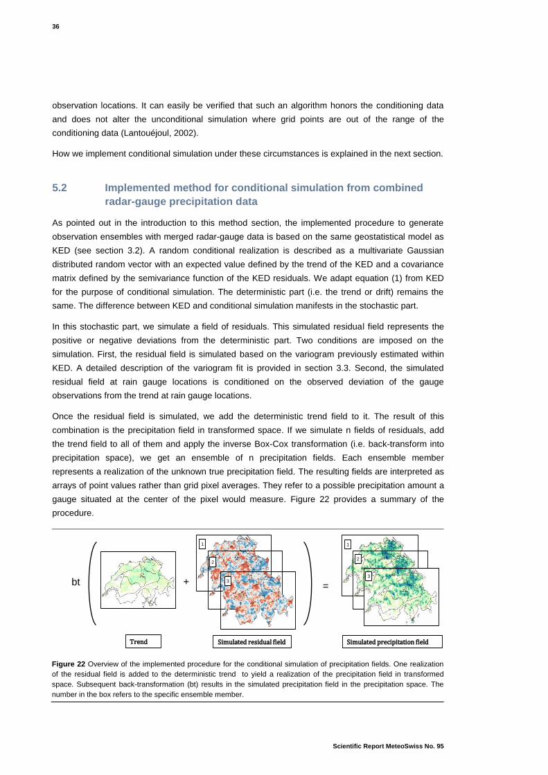
36


observation locations. It can easily be verified that such an algorithm honors the conditioning data

and does not alter the unconditional simulation where grid points are out of the range of the

conditioning data (Lantouéjoul, 2002).

How we implement conditional simulation under these circumstances is explained in the next section.

5.2 Implemented method for conditional simulation from combined

radar-gauge precipitation data

As pointed out in the introduction to this method section, the implemented procedure to generate

observation ensembles with merged radar-gauge data is based on the same geostatistical model as

KED (see section 3.2). A random conditional realization is described as a multivariate Gaussian

distributed random vector with an expected value defined by the trend of the KED and a covariance

matrix defined by the semivariance function of the KED residuals. We adapt equation (1) from KED

for the purpose of conditional simulation. The deterministic part (i.e. the trend or drift) remains the

same. The difference between KED and conditional simulation manifests in the stochastic part.

In this stochastic part, we simulate a field of residuals. This simulated residual field represents the

positive or negative deviations from the deterministic part. Two conditions are imposed on the

simulation. First, the residual field is simulated based on the variogram previously estimated within

KED. A detailed description of the variogram fit is provided in section 3.3. Second, the simulated

residual field at rain gauge locations is conditioned on the observed deviation of the gauge

observations from the trend at rain gauge locations.

Once the residual field is simulated, we add the deterministic trend field to it. The result of this

combination is the precipitation field in transformed space. If we simulate n fields of residuals, add

the trend field to all of them and apply the inverse Box-Cox transformation (i.e. back-transform into

precipitation space), we get an ensemble of n precipitation fields. Each ensemble member

represents a realization of the unknown true precipitation field. The resulting fields are interpreted as

arrays of point values rather than grid pixel averages. They refer to a possible precipitation amount a

gauge situated at the center of the pixel would measure. Figure 22 provides a summary of the

procedure.

Figure 22 Overview of the implemented procedure for the conditional simulation of precipitation fields. One realization

of the residual field is added to the deterministic trend to yield a realization of the precipitation field in transformed

space. Subsequent back-transformation (bt) results in the simulated precipitation field in the precipitation space. The

number in the box refers to the specific ensemble member.

Trend

1

2

3

Simulated residual field Simulated precipitation field

1

2

3

= + bt

37




5.3 Discussion of characteristics of the generated observation

ensembles

As the true precipitation field is unknown, we cannot truly evaluate the plausibility of the observation

ensembles generated. In some studies (e.g. Clark and Slater, 2006), cross validation was used to

analyze the estimation quality of conditional simulation. We already evaluated the reliability of the

cross-validated probabilistic estimates from KED in section 4. Here, we check whether the

ensembles reproduce the prescribed spatial characteristics. We can also modify specific model

settings and investigate their influence on the uncertainty in the observation ensembles.

5.3.1 Technical verification of generated observation ensembles

We verify the technical implementation of the conditional simulation procedure in two ways. First, we

check whether the estimated fields reproduce the underlying variogram, i.e. the variogram fitted to

the original data. We take a random sample of 500 grid points spread all over Switzerland, fit an

exponential variogram to the sample with MLE and compare the fitted to the underlying variogram.

Second, we investigate whether the spread of the ensembles approximates the kriging standard

spread for increasing numbers of simulations. We use the following robust spread measure (r.sd):

( ) (10)

where Q84 and Q16 are the 84% and the 16% quantiles of the ensembles. This choice is motivated

by the skewed nature of precipitation data. For an infinitely big ensemble, the differences between

the ensemble and kriging spread should vanish. We compute the differences to kriging with

ensembles of 10, 100, 200 and 500 members. These experiments also provide insight about the

number of ensemble members needed to appropriately describe the uncertainties.

5.3.2 Comparison of spatial uncertainty

Whether the generated observation ensembles plausibly reproduce spatial uncertainties in

precipitation fields is investigated here. We study the influence of the network density, the

precipitation situation, the ensemble size, the temporal resolution and the addition of radar

information.

The uncertainty experiments are based on the mean areal precipitation of a catchment. For every

ensemble member, the areal means of the Reuss and the three nested sub-catchments of

decreasing size, Reuss Luzern, Urner Reuss and Schaechenbach (see Figure 23), are calculated.

We use the robust spread measure r.sd normalized with the median of the ensembles as measure of

relative spatial uncertainty.

We performed the following experiments:

• Conditional simulation from combined radar-gauge data (CSCOMB) with 100 ensemble members

and the SMN station network for three different days (8 August 2007 (stratiform precipitation), 10

June 2008 (isolated convective precipitation) and 6 September 2008 (overall convective

precipitation))

38


• CSCOMB with the SMN network for 10 June 2008 with 10, 50, 100, 200 and 500 members

• CSCOMB and conditional simulation from gauge data only (CSGAU) with 100 members for all the

example days and the station networks ALL and SMN

• CSCOMB with 100 members and the SMN network for monthly sums of daily precipitation in

January, May and July 2008

For ease of understanding, we again introduce a nomenclature for the different conditional simulation

settings compared. CSCOMB_all and CSCOMB_smn refer to the conditionally simulated observation

ensembles generated with merged radar-gauge data and the station networks ALL and SMN.

Ensembles from conditional simulation of gauge observations only are referred to as CSGAU_all and

CSGAU_smn respectively.

5.4 Software

The software used is the same as in section 3.5. For the conditional simulation of the residuals, we

us an additional R-package called RandomFields (Schlather, 2001).

Figure 23 Location of the Reuss catchment in Central Switzerland. The detail shows the borders of the Reuss

catchment and the nested sub-catchments.

39



6 Results from simulated observation ensembles

6 Results from simulated observation

ensembles

Results from the conditional simulation experiments are presented here for three example days. The

chosen example days represent characteristic precipitation situations encountered in Switzerland

and are described in section 2.2. The chapter is structured as follows. Section 1 discusses the

technical verification of generated observation ensembles. Exemplary precipitation fields from

conditional simulation are shown in section 2. The last section is dedicated to experiments about the

influence of different method settings on the spatial uncertainty in the ensembles.

6.1 Technical verification of the ensembles

Results from investigations whether the generated observation ensembles comply with the

underlying geostatistical model are presented here. Firstly, we show whether the spatial covariance

in the simulated precipitation fields reproduce the underlying variograms, i.e. the variograms that

were estimated from the original data. Secondly, we discuss if the ensemble spread at the grid point

scale reproduces the uncertainty distribution implied by the underlying stochastic concept (i.e. the

spread implied by the kriging standard spread). All the simulations of this technical verification are

performed with CSCOMB_smn. CSCOMB_smn serves as an example for illustration.

In order to investigate the reproduction of the spatial covariance structure in the simulated residual

fields, we took ten ensemble members of CSCOMB_smn. From each of the ten members, we take

five random samples of 500 points. We fit to all of this 50 sets of 500 synthetic stations an

exponential variogram. The distribution of the fitted variogram parameters partial sill and nugget are

shown in Figure 24 for all the three example days.

For the estimated partial sills, we find a spread of the fitted values on all the example days. On the 10

June 2008, the median of the 50 variograms slightly deviates from the underlying partial sill

(represented by the black cross). Overall, we argue the spread and the small deviations of the

median from the underlying partial sill to be in line with the random deviations we would expect.

There is a spread of the fitted nuggets on all the example days. However, no systematic deviation of

the fitted nuggets from the underlying nugget is indicated. We again suggest the findings to be within

the scope of random fluctuations.

The range was reproduced perfectly for all the ensemble members, samples and days (not shown).

The implemented conditional simulation procedure therefore seems to have particular strength in

reproducing the underlying range over which observations are correlated.

40


How do we interpret the perfect reproduction of the range in contrast to the considerable spread of

estimated partial sills and nuggets? We can imagine this to be related to the variogram fitting

technique used here, which tends not to reject the supplied initial value from the empirical variogram

for the range. Nevertheless, the random deviations observed between the estimated partial sills and

nuggets are not contradicting our expectations. The simulated precipitation fields, moreover, are

never used individually. For the following investigations and in applications using conditional

simulation, we always consider an independent ensemble of simulated precipitation fields. We

therefore view the ability of the ensembles to represent the spatial covariance structure of the original

data as verified.

We now turn towards the analysis of the standard spread between the simulated precipitation fields

in the ensembles. Figure 25 shows the robust standard spread r.sd (see equation (10)) of the

ensembles from CSCOMB_smn on the 8 August 2007 for ensemble sizes of 100, 200 and 500

members. The kriging r.sd is shown, too. As expected, the ensemble spread approaches the kriging

spread more and more with increasing numbers of simulations. The basic spatial structure of the

spread is already captured with 100 simulations. However, there is still a lot of small-scale variance

Partial sill

Nugget

Figure 24 Boxplots of the fitted variogram parameters partial sill and nugget for the three example days. Exponential

variograms were fitted with MLE to ten ensemble members from CSCOMB_smn at five random samples of 500 points.

The boxplots show the distribution of the fitted variogram parameters from these 50 variograms. The black cross

represents the underlying variogram parameter of CSCOMB_smn on the specific day.

41




in the ensemble spread. This small-scale variance is strongly but not entirely removed in the

ensemble with 500 members.

We understand this approximation as follows. The simulated ensemble can reproduce the theoretical

spread (inferred from the kriging standard spread) only with limited accuracy when the size of the

ensemble is small. A small ensemble under-samples the joint pdf, which reflects in a noisy variation

of r.sd between neighboring grid points. An ensemble with 500 realizations, however, reproduces the

pattern and magnitude of the theoretical spread accurately, confirming the technical consistency of

the simulation approach with the underlying stochastic model.

Further peculiarities are the distinct minima of the spread around gauge locations represented in all

the four plots. We expect to find those minima due to the conditioning of the simulation on the gauge

observations. Since the covariance over short distances is high, the scope for random deviations is

smaller close to the gauges. The variance between the ensemble members is therefore small. A last

point we want to highlight is that we show the absolute spread in physical (i.e. untransformed) space

here. The back-transformation leads to large spreads in regions with intense precipitation (see Erdin

et al., 2012). We therefore interpret the maxima in spread in the north of Lake of Biel and around the

Lake of Thun as products of two different processes. These processes are first, the lack of a rain

gauge in near proximity and second, the high amount of precipitation realized there.

Ensemble r.sd (n=100)



Kriging r.sd

Figure 25 Ensemble r.sd from CSCOMB_smn for ensembles of 100, 200 and 500 members and kriging r.sd from

KED_smn on the 8 August 2007 in mm. The robust spread measure r.sd is defined in equation (10). See Figure 2 for an

illustration of the precipitation situation on the 8 August 2007.

42


To highlight the deviations of the ensemble and the kriging standard spread, we show their

differences in Figure 26 for ensembles of 10, 100 and 500 members. Positive (blue) values indicate

regions where the spread in the ensembles is bigger than the kriging spread. As pointed out before,

the differences between ensemble and kriging r.sd are reduced when the ensemble size is

increased. The reduction is particularly strong when increasing the number of ensemble members

from 10 to 100. In all the plots, the positive and negative deviations are spread all over the domain.

They are correlated in close proximity with a lot of small-scale variance. This correlation originates

from the spatial correlation. The small-scale variance, too, stems from the nugget in the original data

and was already seen in the ensemble r.sd. The nugget effect, i.e. the strong small-scale variance

caused by the nugget, will be supported when we look at the other example days afterwards.

The eastern part of the Grisons shows the random nature of positive and negative differences

between the ensemble and the kriging spread: the sign changes between the ensemble sizes. The

differences are, however, related to maxima and minima of the spread. As the intensity of

precipitation and thus, the model spread are quite uniform here, these maxima and minima are not

very pronounced. Nevertheless, the reduced difference of ensemble and kriging r.sd in the Grisons

(i.e. the region where the model spread is particularly small) is visible.

Up to now, we focused on the 8 August 2007 in this discussion of the spread in the observation

ensembles. The two convective days, i.e. the 10 June 2008 and the 6 September 2008, reflect what

n=10

n=100

n=500

Figure 26 Differences between the ensemble and kriging r.sd for ensembles of 10, 100 and 500 members on the 8

August 2007 in mm.

43




we have found for the day of stratiform precipitation. For the sake of completeness, we provide a

short discussion and show figures of ensemble and kriging r.sd for both convective days in the

appendix section A.

Summing up the above results, we find the spatial covariance structure imposed by the underlying

variogram to be well reproduced in the ensembles. The spread of the simulated ensembles with

many ensemble members reflects the theoretical model spread well. Our technical implementation of

the conditional simulation procedure is hence verified to be successful. We suggest these findings to

be transferable to ensembles generated with the single-sensor reference and the dense station

network. With a well-justified confidence in the simulated fields we go about to investigate the

generated precipitation fields.

6.2 Precipitation fields from conditional simulation

The chosen example days (see Figure 2 and section 2.2) are used to illustrate how precipitation

fields from conditional simulation actually look like. Here, we point out the differences between

conditional simulation and the best estimates from kriging, and show qualitatively how strong the

random deviations between the individual ensemble members are. The 10 June 2008 is selected for

in-depth discussion as it highlights many remarkable features of conditional simulation and was

already discussed as example case in section 4.2.1. For the remaining two example days, we briefly

point out the important peculiarities and refer to the appendix (section B) for the figures and a more

detailed description.

Figure 27 shows the precipitation fields from kriging (i.e. the field of best estimates) and conditional

simulation for the combination and the single-sensor reference method with both station networks.

For comparability, the radar composite with the rain gauge measurements from the dense station

network is shown in Figure 2. In the best estimates, areas with the same precipitation amount

estimated are larger than in the realizations from conditional simulation. All the ensemble members

from CSCOMB and CSGAU for both network densities have a higher spatial variability of

precipitation than the corresponding best estimates. The fields of best estimates are therefore much

smoother than the simulated precipitation fields. A comparison between the combination and the

single-sensor reference accentuates the strong increase in the variability of precipitation from

OKGAU to CSGAU. The best estimates of OKGAU with both station densities are very smooth. The

ensemble members from CSGAU, however, have a spatial variability representing the spatial

covariance structure of the original data. The increase in spatial variability from the best estimates to

the simulated fields of the combination (KED to CSCOMB) is less pronounced. The inclusion of radar

as an external drift variable leads to considerable spatial variability already in the field of best

estimates. Still, the increase in small-scale variability of precipitation in the ensemble members is

clearly discernible. The quantitative differences between the precipitation fields OKGAU and CSGAU,

however, do not imperatively have to be bigger than the differences between KED and CSCOMB.

44


OKGAU_smn

CSGAU_smn

OKGAU_all

CSGAU_all

KED_smn

CSCOMB_smn

KED_all

CSCOMB_all

Figure 27 Best estimate fields of precipitation (in mm) from kriging (left) and one ensemble member from conditional

simulation (right) on the 10 June 2008. Precipitation fields are shown for the single-sensor reference method (OKGAU

and CSGAU) and the combination method (KED and CSCOMB) for both network densities.

45




Conditional simulation produces local extremes beyond the range of the observations. More frequent

are both areas where very intense (e.g. the Lake of Zurich area) and spots where no precipitation at

all (e.g. the Valais) is simulated. The additional radar information in CSCOMB seems to increase the

likeliness of extreme precipitation over 90 mm. We would expect this behavior, since the trend field

from radar includes maxima lying between the stations. These maxima are not reproduced in

simulated precipitation fields from CSGAU with a constant underlying trend corresponding to the

mean of the rain gauge observations.

Comparing fields using the sparse and the dense station network for model estimation and

conditioning, we find the additional climatological gauges to lead to an increase in small-scale

variability. We understand this from the differences in the nugget between the dense and the sparse

station network. Whilst CSCOMB_smn and CSGAU_smn both have a nugget of zero, the nugget-to-

sill ratios are more than 0.3 and 0.2 for CSCOMB_all and CSGAU_all respectively. This renders the

simulated precipitation fields spottier. (A nugget of zero is more frequently realized when using the

sparse station network due to the implemented variogram modeling procedure).

The example demonstrates the differences between the fields of the best estimates and realizations

from conditional simulation. The best estimates indicate for every grid point the values which have on

average the least squared deviation from the true (but unknown) precipitation field. This implicitly

entails a smoothing of the precipitation field. The best estimates therefore clearly miss small-scale

variations present in the original data. If a variogram was estimated from such a field of best

estimates, the variance would be much smaller than the variance present in the original data.

Precipitation fields from conditional simulation retain this variance. The simulated ensemble

members are all equally probable and represent potentially true precipitation fields. In these

precipitation fields, extremes are represented exceeding the range of the gauge observations and, in

case of the combination, the adjusted radar information.

It is difficult to assess whether the small-scale structure evident in the simulation for the 10 June

2008 from CSCOMB_all is truly realistic for a precipitation field. Indeed, the comparatively large

nugget could be a manifestation of the limited spatial representativity of the gauge measurements. In

this case the variations from one grid point to the next contain a component of variation that is due to

variations at very small scales (including random measurement errors). The construction of our

simulation system via point measurements in fact presumes that the resulting fields are interpreted

as an array of point values (say the measurements at rain gauges located at the center of the grid

pixels), rather than a field of areal averages over the grid pixels.

Four ensemble members from CSCOMB_smn are shown in Figure 28. They obviously look very

similar. The underlying spatial covariance structure and the values at gauge locations are by

definition the same. What makes the individual ensemble members unique are their random

deviations in between rain gauge locations. As shown in Figure A1 of the appendix, these deviations

(i.e. the r.sd) are largest where precipitation is most intense. An example of a region where the

ensemble members strongly deviate from each other is in between the lakes of Zurich and Zug.

Whilst member a) has a strong maximum with precipitation reaching up to 120 mm, ensemble

member d) does not show a distinct maximum in this region.

46


Subtracting the trend from the precipitation fields, Figure 30 shows the simulated residual fields (i.e.

the stochastic component of the underlying geostatistical model) in the transformed space. CSCOMB

and CSGAU with both station densities all have a different trend field. As the residuals at gauge

locations are computed from the difference between gauge observations and trend estimate at the

same location, they depend on the trend field. We therefore cannot compare the locations of positive

and negative values of the simulated residual field among the different methods. What we can

compare are the spatial characteristics of the simulated residual fields.

The simulated residual fields from CSGAU show much more large-scale variation. Independent of

the network density and the specific ensemble member, the residuals at gauge locations and thus

the simulated residual fields are in general negative (i.e. the trend is corrected downwards) in the

Valais and positive around the lake of Zurich. We expect this behavior, since the trend field from

CSGAU corresponds to the mean of the gauge observations. The simulated residual field therefore

corrects the trend upward in wet and downward in dry regions. With CSCOMB, this large-scale

variation is in the form of the radar information already included in the trend field. The simulated

residuals from CSCOMB therefore do not show this large-scale variation pattern.

Comparing the simulated residuals generated using the sparse and the dense station network, we

again see the nugget effect causing a lot of small-scale variability in the simulated residual fields of

CSCOMB_all and CSGAU_all. The nugget effect is more clearly visible if we consider the simulated

residual field alone, i.e. without the additional trend. Having a nugget of zero in the original data, both

CSCOMB_smn and CSGAU_smn do not show this small-scale variance.

a)

b)

c)

d)

Figure 28 Four ensemble members from CSCOMB_smn on the 10 June 2008. Precipitation is given in mm.

47




CSGAU_smn 1

CSGAU_smn 2

CSGAU_all 1

CSGAU_all 2

CSCOMB_smn 1

CSCOMB_smn 2

CSCOMB_all 1

CSCOMB_all 2

Figure 29 Two realizations of the simulated residual field in transformed space on the 10 June 2008 with CSGAU and

CSCOMB for both network densities.

48


If we make the comparison between the two members of the same method, we see that they seem to

differ more strongly for the sparse station network. The members of CSCOMB_all and CSGAU_all

both show fairly similar simulated residual fields. We interpret this such that the uncertainty about the

true precipitation field is smaller when the dense station network is used. Due to the strength of the

small-scale variance, however, differences between members are hard to make out and we rather

wait for section 6.3 to make statements regarding the uncertainty in the estimates.

The 8 August 2007 is our example day of stratiform precipitation. The day is characterized by large

radar errors. This is reflected in the uniform trend fields of CSCOMB, very similar to the constant

mean trend of CSGAU (not shown). The relatively large nugget observed manifests in the simulated

precipitation fields, too. The question, whether a precipitation field with this strong small-scale

variance meets the expectations about a stratiform precipitation field, is pending. The mentioned

issues are illustrated and elaborated in detail in section B of the appendix.

The last example day to be discussed is the 6 September 2008. This day is characteristic for an

overall convective precipitation situation with an intense local maximum of precipitation in the Ticino.

With conditional simulation, the representation of this local maximum in the ensembles is worth a

discussion. Moreover, the fate of the radar stripes visible in Figure 2 needs to be investigated. Details

on the above are provided in section B of the appendix.

6.3 Experiments for quantifying the uncertainty reduction attributable

to different method settings

The previous sections of this chapter highlight the differences of the three example days. Here we

want to investigate how these differences condense quantitatively in the spread of the mean areal

precipitation of the ensembles. The Reuss catchment is used for this quantification (see Figure 23).

Before we dive into the different experiments, it should be noted that we just show examples and do

not perform a systematic analysis here. This section rather serves to illustrate what opportunities

conditional simulation offers than to claim representativeness. Nevertheless the results provide

exemplary insight into the variation and dependency of estimation uncertainty and serves as a

qualitative plausibility assessment of the simulation concept.

Figure 30 shows the relative spatial uncertainty (i.e. the estimated uncertainty in our model

represented by the spread between the ensemble members) of the mean areal precipitation in

ensembles of 100 members simulated with CSCOMB_smn. On all the example days, the spread

between the ensemble members increases for decreasing catchment size. For intuition, a relative

spread (i.e. the r.sd (equation (10)) normalized with the median; see Table 5) of 0.483 for

Schaechenbach corresponds to an r.sd of 6.24 mm (at a median of 12.9 mm). This reduces to 2.379

mm (at a median of 11.84 mm) for the complete Reuss catchment. We expected to find a reduced

spread of mean areal precipitation in larger catchments and interpret it as being caused by stronger

compensation of the random deviations in catchments of bigger size.

49




The differences between the spread of the different days are considerable. The smallest spread is

achieved on the 8 August 2007, the day with stratiform precipitation. Of the two convective days, the

6 September 2008 (overall convective precipitation) has a lower spread. We interpret the reduced

spread in case of stratiform precipitation as caused by the higher spatial autocorrelation of the

observations manifesting in the larger range (201 km compared to 35 km (10 June 2008) and 140 km

(6 September 2008)). Furthermore, the average precipitation amount estimated on the example day

of stratiform precipitation is higher (see Figure 2), which reduces the relative uncertainties. The

spread between the ensemble members is highest on the day with isolated convective precipitation.

We argue that both the average precipitation and the range are smallest on this day. Precipitation

therefore co-varies only over short distances which increases the random spread. On the level of

mean areal precipitation, the very small-scale and spatially uncorrelated nugget variance is

compensated and thus, no nugget effect is observed.

From a certain catchment size on, a further increase in catchment size does not seem to reduce the

spread any further. The 740 km2 increase from the Schaechenbach to the Urner Reuss catchment

reduces the spread in the areal means more strongly than the 1400 km2 increase from Urner Reuss

to Reuss Luzern. We would expect this behavior, since the relative increase in size is much bigger

from Schaechenbach to Urner Reuss than from Urner Reuss to Reuss Luzern.

Table 5: Relative standard spread of mean areal precipitation of ensembles with 100 members for the four catchments

Reuss, Reuss Luzern, Urner Reuss and Schaechenbach. The relative standard spread is defined as the r.sd normalized

with the median of the respective catchment and method setting. Results from CSGAU and CSCOMB with both network

densities are shown for the 10 June 2008.

Reuss Reuss Luzern Urner Reuss Schaechenbach CSGAU_smn 0.253 0.267 0.360 0.671

CSGAU_all 0.107 0.136 0.262 0.294

CSCOMB_smn 0.201 0.223 0.285 0.483

CSCOMB _all 0.080 0.094 0.192 0.266

Figure 30 Boxplots of mean areal precipitation for the four catchments Reuss (3431 km2), Reuss Luzern (2261 km

2),

Urner Reuss (847 km2) and Schaechenbach (106 km

2). Results from CSCOMB_smn with 100 ensemble members are

shown for the three example days. The areal means are normalized with the median of the respective catchment and

day.

50


Concentrating on the 10 June 2008, Table 5 shows the relative r.sd of precipitation for the four

catchments with CSCOMB and CSGAU for both network densities. The strongest uncertainty

reduction is achieved with CSCOMB_all, followed by CSGAU_all and CSCOMB_smn. Most

uncertainty regarding the true precipitation field is in simulations with CSGAU_smn. Bringing the

results of the best estimates back into mind, we see that the improvement of the combination and the

single-sensor reference with both network densities is similar for both the accuracy of the point

estimates (kriging) and the spatial uncertainty in the ensembles (conditional simulation). First, 360

additional gauges are more successful in reducing the spatial uncertainty than the radar information.

Second, CSCOMB reduces the spatial uncertainty compared to CSGAU with the same station

network. Third, the additional radar information tends to reduce the spread more strongly if we use

the sparse station network. The radar information in this example, hence, successfully reduces the

spatial uncertainty of mean areal precipitation. These results demonstrate that our conditional

simulation technique plausibly reproduce the uncertainty of the estimates.

Figure 31 illustrates the spread in the areal means for the different catchments with boxplots for all

the example days. On top of the information from Table 5, we see in the boxplots that CSGAU tends

to have more outliers than CSCOMB on the 10 June 2008. Especially CSCOMB_all seems to be

outlier-free.

Looking at the 6 September 2008, we draw the same conclusions concerning the level of uncertainty

in the simulated precipitation fields. CSCOMB_all exhibit the lowest and CSGAU_smn the highest

uncertainty in the ensembles. CSCOMB_all has some outliers observed on this day, too. We

interpret these outliers observed with CSCOMB and CSGAU with both network densities as a

characteristic of conditional simulation to simulate both extremely low and extremely high

precipitation.

On the 8 August 2007, the benefit of radar information is not apparent. The spread of CSCOMB is

not systematically smaller than the spread of CSGAU. With the dense gauge network the simulated

fields have lower spread than with the sparse SMN network. This result is indicated by the low βs

(see Figure 2) on this day. We suggest, again, radar information to be particularly beneficial in case

of convective precipitation. Whereas for stratiform (spatially more coherent) precipitation patterns, a

dense gauge network is more decisive for estimating catchment mean precipitation.

In section 6.1 the differences between the ensemble and kriging standard spread are analyzed. We

saw that many realizations are required to approach the theoretical model spread (i.e. the kriging

spread) by the ensembles. Here we undertake an experiment to examine the sensitivity with respect

to ensemble size of catchment mean precipitation. Results are shown in Figure 32. We see that the

spread varies with different ensemble sizes. The spread confined by the whiskers of the boxplot

increases for increasing ensemble sizes in both catchments. Yet, interquartile range (i.e. the size of

the box) for Reuss Luzern is overestimated in small ensembles and remains constant for ensembles

with 100 and more members. On the contrary, the interquartile range increases from 10 to more

ensemble members for the Schaechenbach catchment. The really extreme precipitation (represented

by the outliers) only becomes abundant in ensembles with more than 100 members. This is due to

the better sampling of the skew pdf. The outliers with extremely low precipitation are missing. Since

we saw ensemble members with extremely low precipitation represented in Figure 31, we do not

expect the issue to be systematic.

51




We would expect the spread of the larger catchment (Reuss Luzern) to be well approached with

fewer simulations than it is the case for the smaller catchment (Schaechenbach). Indeed, the spread

seems not to vary too much for increasing ensemble sizes in the larger catchment. For extreme

values to be simulated, however, it still needs more than 200 ensemble members. Since results from

one single experiment are presented, a generalization of these findings is difficult. Nevertheless,

considering that this convective case represents more demanding conditions, a minimum of 100

members is a reasonable requirement for catchment sizes larger than 100 km2.

10 June 2008

8 August 2007

6 September 2008

Figure 31 Boxplots of areal mean precipitation for the four catchments Reuss, Reuss Luzern, Urner Reuss and

Schaechenbach on the three example days. Results from CSGAU and CSCOMB with both network densities with 100

ensemble members are shown. The areal means were normalized with the median of the respective catchment, day

and method setting. Note that the scale changes for the different days.

52


Up to now, we only considered precipitation on the daily time scale in this plausibility assessment.

Figure 34 shows how the aggregation of daily precipitation fields over a whole month reduces the

uncertainty in the precipitation estimates. With the monthly aggregation, the spread observed in the

daily estimates is reduced. We would expect this behavior, since the increased time scale over which

the simulated precipitation fields are aggregated is suggested to have a similar effect as the

increased area over which precipitation is averaged. As the ensemble members are temporally

independent, random daily deviations compensate each other in a monthly aggregation. We did not

perform a systematic analysis of the influence of the time scale though. The comparison here is

made between arbitrary example months and days. No interpretation on the magnitude of the

uncertainty reduction from the increased time scale can be provided.

Figure 32 Boxplots of areal mean precipitation for the two catchments Reuss Luzern and Schaechenbach on the 10

June 2008. Results from CSGAU_smn with 10, 50, 100, 200 and 500 ensemble members are shown. The areal means

were normalized with the median of the respective catchment and ensemble size.

Figure 33 Boxplots of areal mean precipitation for the four catchments Reuss, Reuss Luzern, Urner Reuss and

Schaechenbach on the three example months January, May and July 2008. Results from CSGAU_smn with 100

ensemble members are shown. The areal means were normalized with the median of the respective catchment and

month.

53




If we compare the spread of the different catchments, we see that the spread is biggest in the

Schaechenbach catchment with an uncertainty of 10 - 20% (interquartile range) depending on the

considered month. The three larger catchments have much smaller and more similar spreads. Also

the difference between the three months is biggest for the Schaechenbach catchment. We argue that

an aggregation over 31 days cannot compensate the strong random deviations observed in such a

small catchment.

The month May 2008 has the biggest spread for the Schaechenbach catchment and more outliers

than the other two months. May 2008 is an example of a month where a few days of intensive

precipitation made up for most of the precipitation fallen during the entire month. We therefore

suggest the increased spread to be caused by the relatively strong influence of the uncertainty of the

days with very intense precipitation, preventing a strong compensation of random daily deviations by

the monthly aggregation. The two other months have a more uniform distribution of precipitation

among the individual days of the month.

54


7 Conclusions

In this thesis we have investigated a statistical technique of radar-gauge combination to produce

precipitation estimates in Switzerland that include measures of the pertinent analysis uncertainty.

The methodology builds on a geostatistical simulation framework, which delivers an ensemble of

precipitation fields that are all consistent with the measurements (conditional simulation). Compared

to the conventional target of one ‘best estimate’, the ensemble technique provides a fully probabilistic

estimate of the observed precipitation distribution. This is particularly suitable in applications that

require realistic spatial structures in precipitation fields and where the consideration of uncertainties

is crucial (e.g. in runoff modeling). The thesis has focused on daily precipitation totals in Switzerland.

It has thoroughly evaluated the geostatistical methodology (kriging with external drift; KED),

assessed the reliability of the ensembles, and examined sensitivities with respect to the rain gauge

network density.

The combination represents a substantial improvement over precipitation estimates from more

traditional single-sensor methods. The accuracy of the rain gauge measurements and the high

resolution of the radar information are successfully brought together. The systematic bias is strongly

reduced compared to the radar reference. In particular, the strong geographic bias due to

underestimation in the mountainous regions and overestimation in the Swiss Plateau is removed.

The combination shows particular skill when it comes to distinguishing wet and dry areas. In

convective precipitation situations the benefit of the additional radar information is specifically strong:

the skill measures of the combination are particularly high in summer, when convective precipitation

is abundant. The combination used is able to both take advantage of the radar information when it is

beneficial and avoid potential negative influences when radar information is erroneous. Similar

results were found in comparable studies using the same combination technique in Switzerland for a

case study of daily precipitation (Erdin, 2009) and a systematic analysis of hourly precipitation

(Keller, 2012). The results are in line with a study by Schuurmans et al. (2007) that found KED to

produce more accurate daily precipitation estimates than single-sensor methods. Goudenhoofdt and

Delobbe (2009) also find radar benefits to be particularly significant in summer.

As in Erdin (2009), the added value of the combination is sensitive to the rain gauge network density.

The increase in skill of the combination over a rain gauge only reference is twice as high when the

sparse SMN network is used. Since the automatic SMN stations have a ten minute time resolution,

the combination is particularly interesting on short time scales and in real-time applications. Another

feature where the combination improved the quality of the best estimates is the representation of

intense precipitation. Precipitation exceeding predefined thresholds is less often classified as

extremely unlikely by the cross-validated probabilistic estimate of the combination. This signalizes a

better representation of intense precipitation by the combination, which is useful in applications of

conditional simulation.

A particularly interesting finding is that greater improvement in the quality of the best estimates can

be achieved through additional information from the 366 climatological gauges, rather than from

radar data. The skill and the reliability of the precipitation estimates are systematically higher when

the dense gauge network is used. This is an important result of the systematic evaluation. In a first

55



7 Conclusions

case study restricted to five example days (Erdin, 2009), adding radar information to a sparse gauge

network was found to be more beneficial compared to adding information from a denser gauge

network. Also Haberlandt (2007) find the addition of radar information to hourly precipitation

observations from 21 automatic gauges to be more important than additional information of 281

climatological gauges on the total rainfall sum of a four day flood event in Germany. Unfortunately, a

comparison of our results to Haberlandt (2007) is possible only to a limited extent. Information from

the climatological gauges cannot be used one-to-one on the hourly time scale and radar data quality

in Switzerland suffers from the shadowing of mountains, unlike in Germany.

Illustrative example cases demonstrate that the conditional simulation technique can plausibly deal

with the uncertainties in the estimates. The variations and dependencies of the estimation uncertainty

are plausibly reproduced in the simulated ensembles. Additional information from a denser rain

gauge network, for example, leads to a stronger reduction of the pertinent uncertainty. Also the

additional radar information in the combination and both spatial and temporal aggregation reduce the

uncertainty in the precipitation estimates. An issue worth discussing is the number of simulations to

be performed in order to represent the theoretical model spread (inferred by the kriging standard

spread) adequately. We could show that for a good representation of both theoretical spread and

extremes at single grid points, at least 100 ensemble members are needed. Previous studies use

ensemble sizes of 25 (Germann et al., 2009), 40 (Ekström et al., 2007) or 100 members (Ahrens and

Jaun, 2007). Here it appears that ensembles with less than 100 members cannot properly reflect the

theoretical model spread. Yet, the plausibility assessment indicates the required ensemble size to be

sensitive to spatial aggregation and the precipitation situation. In small catchments it thus requires

ensembles of bigger size to adequately reproduce the theoretical model spread.

Our combination approach incorporates two major limitations. First, we assume the rain gauges to

represent the correct value of precipitation at their respective locations. Both the rain gauge and the

radar observations, however, are uncertain. Second, the rain gauge observations are point

measurements, whereas the radar data and, finally, the gridded estimates refer to areal precipitation

of 1 km2. This induces problems of scale compatibility in the combination of radar and gauge data.

We therefore have to be aware that the real uncertainty of precipitation is different or rather higher

than the uncertainty captured in the model.

The presented combination delivers best estimates and ensembles with limited precision. The

precision can be improved either through advances regarding the observational monitoring system or

by methodological developments. MeteoSwiss is undertaking efforts to reduce limitations of the

observational monitoring system. The density of the automatic gauge network is being increased, two

more radars in the Grisons and the Valais are to be installed and the measurement technology

upgraded (MeteoSwiss, 2012; MeteoSwiss, 2010). Concerning methodological developments, we

can think of a number of potential improvements that could be achieved in further investigations. The

regional differences in the quality and the reliability of the estimates are considerable. We have to

raise the question whether the stationarity assumption for the whole territory of Switzerland can be

maintained. Our main argument for a stationarity assumption is the limited availability of observations

and potential robustness problems induced by a small sample. Especially with the climatological

gauge network and in the light of the denser SMN network, region-specific stationarity assumptions

should be examined. Moreover, the strong regional differences in the Bias motivate an investigation

of potential benefits of a regionally varying trend. Thereby, the influence of regions with particularly

56


large radar errors, like Western Switzerland on the 8 August 2007, might be reduced. Since the radar

artifacts could not be entirely removed in the combination, an inclusion of information about radar

quality is appealing. Erdin (2009) attempted to add a radar uncertainty term to the model. Though

unsuccessful, they suggest that a more sophisticated modeling technique should lead to model

improvement. We consider a principal component analysis of radar errors as a potential candidate for

this. As in Keller (2012) and Erdin (2009), radar information is found to be particularly beneficial for

distinguishing between wet and dry areas. This could possibly be exploited by indicator kriging with

radar information used to indicate wet and dry regions, as done by Schleiss et al. (2012).

In contrast to conditional simulation, a series of previous studies was performed using KED and

related kriging techniques in the radar-gauge merging context at MeteoSwiss (e.g. Erdin et al., 2012;

Erdin, 2009; Keller, 2012; Sideris, submitted). Moreover, a combination method is already

operational (Sideris et al., submitted). An open issue is the W-shape of the reliability plots produced

on the daily time scale. The increase in relative frequencies around the median was not observed for

hourly precipitation. A comparison of the hourly and the daily radar-gauge combination product would

be valuable. Due to the longer aggregation period, days requiring a fall-back solution for parameter

estimation are rarer. In the application with the dense gauge network, the variogram and model

parameters are thus expected to be estimated more reliably.

In this first attempt to apply conditional simulation in a radar-gauge merging context, we performed a

case study of three example days characterized by different precipitation situations. First results are

promising and indicate potential for further investigations. We propose to study more example days

to learn about other interesting features of conditional simulation. An investigation of the behavior of

the ensemble spread with the dense station network and the single-sensor reference could be

worthwhile. We just perform conditional simulation with a rain gauge only reference. It would be

interesting to compare the combined ensembles to a single-sensor ensemble from radar. The

implemented procedure of conditional simulation yields arrays of point values rather than areal

averages of grid pixels. For a further development of our simulation procedure to simulate grid pixel

averages, we can think of two interesting options. First, grid pixel averages could be created by

simulating on a high resolution grid (say on a 4x4 pixel subgrid for every pixel of the original grid) and

subsequent averaging to the coarser grid. Second, block kriging provides an interesting framework to

simulate block values instead of point values.

The generated observation ensembles could be used for designing the monitoring and warning

systems. Where the spatial uncertainty of precipitation is high, additional measurement stations are

particularly necessary. A possibility to validate the spatial uncertainty in the simulated precipitation

fields is to feed them into a hydrological rainfall-runoff model (e.g., Germann et al., 2009; Zappa et

al., 2008). This allows for a comparison of both the spread of simulated mean areal precipitation with

the spread of the simulated runoff, and a comparison of the simulated to the observed river runoff.

Although the results are affected by the quality of the hydrological model too, a real world verification

of the spatial uncertainty in the estimates is possible. For example, an investigation of the ability of

the simulated ensembles to forecast river runoff during the heavy precipitation event in August 2005

could provide valuable insight into the performance of conditional simulation in the radar-gauge

merging context.

57



7 Conclusions

Emery and Lantuéjoul (2006) mention limitations of the R-package used for simulation, causing

inefficiencies when covariances are not smooth at the origin or leading to a loss in accuracy of the

covariance reproduction. The technical verification performed shows the simulated precipitation fields

to meet the requirements. Still, the different simulation algorithms implemented in the R-package

RandomFields (e.g., turning bands methods or circulant embedding; see Schlather (2001)) motivate

an investigation whether specific simulation algorithms are advantageous in our framework.

58


Abbreviations

ALL Station network including both automatic SMN and climatological gauges

Bias Systematic error computed on logarithmic scale; skill measure

C() Covariance function

C(0) Total variance (i.e. σ2

n + σ2

ps)

CSCOMB Conditional simulation from combined radar-gauge data

CSCOMB_smn CSCOMB using gauge observations from the SMN station network

CSCOMB_all CSCOMB using gauge observations from the station network ALL

CSGAU Conditional simulation from rain gauge data; single-sensor reference method

CSGAU_smn CSGAU using gauge observations from the SMN station network

CSGAU_all CSGAU using gauge observations from the station network ALL

E Matrix with the eigenvectors in the columns

ek Eigenvector

est Estimation

h Lag; Euclidean distance between two points

HK Hanssen-Kuipers discriminant; skill measure

i, j Indices for spatial reference

KED Kriging with external drift

KED_smn KED using gauge observations from the SMN station network

KED_all KED using gauge observations from the station network ALL

MAD Mean absolute deviation; skill measure

MLE Maximum likelihood estimation

obs Observation

OKGAU Ordinary Kriging of rain gauges; single-sensor reference method

59



Abbreviations

OKGAU_smn OKGAU using gauge observations from the SMN station network

OKGAU_all OKGAU using gauge observations from the station network ALL

P Modeled precipitation amount

pdf Probability density function

QPE Quantitative precipitation estimate

Q Quantile

r Range parameter corresponding to 1/3 of the practical range

RADAR QPE product from radar; single-sensor reference method

r.sd Robust spread measure

Rel. MRTE Relative mean root transformed error; skill measure

REML Restricted maximum likelihood estimation

RHIRES Deterministic spatial interpolation method

S Variance

SCATTER Skill measure

SEEPS Stable equitable error in probability space; skill measure

SMN SwissMetNet; automatic station network

Y Untransformed precipitation data

Y* Transformed precipitation data

x Simulated random vectors

Z Random process or radar reflectivity, depending on the context

α Intercept of linear trend model

β Trend coefficient of linear trend model

γ() Variogram

λ Transformation parameter or eigenvalue; depending on the context

λlower Lower bound of the transformation parameter λ

Σ Covariance matrix

σ2n Nugget

σ2ps Partial sill

60


References

Ahrens, B.; Jaun, S. (2007), 'On evaluation of ensemble precipitation forecasts with observation

based ensembles', Adv. Geosci. 10, 139–144.

Box, G. E. P.; Cox, D. R. (1964), ‘An analysis of transformations’, J. Roy. Stat. Soc., 26A, 211-252.

Clark. M. P.; Slater, A. G. (2006), 'Probabilistic quantitative precipitation estimation in complex

terrain', J. Hydrometeorol. 7, 3–22.

Cressie, N.A.C. (1993), ‘Statistics for Spatial Data’, Wiley, Chichester, 900 pp.

DeGaetano, A. T.; Wilks, D. S. (2008), ‘Radar-guided interpolation of climatological precipitation

data’, Int. J. Climatol. 29, 185–196, doi:10.1002/joc.1714.

Ekström, M.; Kyriakidis, P. C.; Chappell, A. (2007), 'Spatiotemporal Stochastic Simulation of

Monthly Rainfall Patterns in the United Kingdom (1980–87)', J. Climate 20 (16), 4194-4210.

Emery, X., Lantuéjoul, C. (2006), 'TBSIM: a computer program for conditional simulation of three-

dimensional Gaussian random fields via the turning bands method', Comput. Geosci. 32 (10), 1615-

1628.

Erdin, R; Frei, C.; Künsch, H. R. (2012), 'Data transformation and uncertainty in geostatistical

combination of radar and rain gauges', J. Hydrol. 13, 1332-1346.

Erdin, R. (2011), ‘Evaluation guidelines of CombiPrecip’, Internal report, MeteoSwiss, 10pp.

Erdin, R. (2009), 'Combining Rain Gauge and Radar Measurements of a Heavy Precipitation Event

over Switzerland', Veroeffentlichungen der MeteoSchweiz 81, 108 pp.

Frei, C.; Germann, U.; Fukutome, S.;Liniger, M. (2008), 'Möglichkeiten und Grenzen der

Niederschlagsanalysen zum Hochwasser 2005', Arbeitsberichte der MeteoSchweiz 221, 19 pp.

Frei, C.; Schöll, R.; Fukutome, S.; Schmidli, J.; Vidale, P.L. (2006), ‘Future change of precipitation

extremes in Europe: An intercomparison of scenarios from regional climate models’, J. Geophys.

Res. 111, D06105, doi:10.1029/2005JD005965.

Frei, C.; Schär, C. (1998), ‘A precipitation climatology of the Alps from high-resolution rain-gauge

observations’, Int. J. Climatol. 18, 873-900.

Germann, U.; Berenguer, M.; Sempere-Torres, D.; Zappa, M. (2009), 'REAL – Ensemble radar

precipitation estimation for hydrology in a mountainous region', Q. J. R. Meteorol. Soc. 135, 445–

456.

61



References

Germann, U.; Galli, G.; Boscacci, M.;Bolliger, M. (2006), 'Radar precipitation measurement in a

mountainous region', Q. J. R. Meteorol. Soc. 132, 1669-1692.

Goovaerts, P. (1997), ‘Geostatistics for Natural Resources Evaluation’, Oxford University Press,

New York, 483 pp.

Goudenhoofdt, E.; Delobbe, L. (2009), 'Evaluation of radar-gauge merging methods for quantitative

precipitation estimates', Hydrol. Earth Syst. Sci. 13, 195–203.

Haberlandt, U. (2007), 'Geostatistical interpolation of hourly precipitation from rain gauges and radar

for a large-scale extreme rainfall event', J. Hydrol. 332, 144-157.

Keller, D. (2012), ‘Evaluation and comparison of radar-rain gauge combination methods-Scientific

basis for selecting a new real-time precipitation estimation method for Switzerland’, Scientific Report

MeteoSwiss 94, 80 pp.

Krajewski, W. F. (1987), 'Cokriging radar-rainfall and rain gage data', J. Geophys. Res. 92, 9571-

9580.

Lantuéjoul, C. (2002), 'Geostatistical Simulation. Models and Algorithms', Springer, Berlin, 256 pp.

Leuenberger, D., Rossa, A. (2007), ‘Revisiting the latent heat nudging scheme for the rainfall

assimilation of a simulated convective storm’, Meteor. Atmos. Phys. 98, 195–215.

MeteoSwiss (2012), ‘Annual Report 2011', Federal Office of Meteorology and Climatology

MeteoSwiss, 40 pp.

MeteoSwiss (2010), 'An observation network for the future’, Federal Office of Meteorology and

Climatology MeteoSwiss, 7 pp.

R Development Core Team (2011), 'R: A language and environment for statistical computing’, R

Foundation for Statistical Computing, Vienna, Austria, ISBN 3-900051-07-0, URL www.Rproject.org.

Rakovec, O.; Hazenberg, P.; Torfs, P. J. J. F.; Weerts, A. H.; Uijlenhoet, R. (2012), ‘Generating

spatial precipitation ensembles: impact of temporal correlation structure’, Hydrol. Earth Syst. Sci. 16,

3419–3434.

Ribeiro Jr., P.J.; Diggle, P.J. (2001), 'geoR: A package for geostatistical analysis', R-NEWS 1 (2),

15-18. ISSN 16093631.

Rodwell, M. J.; Richardson, D. S.; Hewson, T. D.; Haiden, T. (2010), ‘A new equitable score for

verifying precipitation in numerical weather prediction’, Q. J. R. Meteorol. Soc. 136, 1344-1363.

Seo, D.-J. (1998), 'Real-time estimation of rainfall fields using radar rainfall and rain gage data', J.

Hydrol. 208, 37-52.

Scherrer, S. C.; Frei, C.; Croci-Maspoli, M.; Van Geijtenbeek, D.; Hotz, C.; Appenzeller, C.

(2011), ‘Operational quality control of daily precipitation using spatio-climatological plausibility

testing‘, Meteorol. Z. 20 (4), 1-11.

Schlather, M. (2001), 'Simulation of stationary and isotropic random fields', R-News, 1 (2), 18-20.

62


Schleiss, M.; Jaffrain, J.; Berne, A. (2012), 'Stochastic Simulation of Intermittent DSD Fields in

Time', J. of Hydrometeorol. 13, 621-637.

Schuurmans, J. M.; Bierkens, M. F. P.; Pebesma, E. J.; Uijlenhoet, R. (2007), 'Automatic

Prediction of High-Resolution Daily Rainfall Fields for Multiple Extents: The Potential of Operational

Radar', J. Hydrometeorol. 8, 1204–1224.

Sevruk, B. (1985), ’Correction of precipitation measurements, summary report’, Proceedings of the

ETH:IAHS:WMO Workshop on the Correction of Precipitation Data, 13–23.

Sideris, I., Gabella, M.; Erdin, R.; Germann, U. (submitted), ‘Real-time radar-raingauge merging

using spatiotemporal co-kriging with external drift in the alpine terrain of Switzerland’, Q. J. R.

Meteorol. Soc.

Talagrand, O.; Vautard, R., Strauss, R. (1997), ‘Evaluation of probabilistic prediction systems’,

Proc. ECMWF Workshop on Predictability, Shinfield Park, United Kingdom, ECMWF, 1–25.

Webster, R.; Oliver, M. A. (2007), ‘Geostatistics for Environmental Scientists’, Wiley, Chichester,

315 pp.

Viviroli, D.; Mittelbach, H.; Gurtz, J.; Weingartner, R. (2009), ‘Continuous simulation for flood

estimation in ungauged mesoscale catchments of Switzerland – Part II: Parameter regionalisation

and flood estimation results’, J. Hydrol. 377, 208–225.

Wilks, D. (2006), ‘Statistical Methods in the Atmospheric Sciences’, Elsevier, Amsterdam, 627 pp.

Young, C.; Bradley, A.; Krajewski, W.; Kruger, A.; Morrissey, M. (2000), ‘Evaluating NEXRAD

multisensor precipitation estimates for operational hydrologic forecasting’, J. Hydrometeor. 1, 241–

254.

Zappa, M., and Coauthors (2008), ‘MAP D-PHASE: Real-time demonstration of hydrological

ensemble prediction systems’, Atmos. Sci. Lett. 9, 80–87.

63



Acknowledgement

Acknowledgement

With all due thunder and fanfare I would like to express many thanks to my supervisors. I want to

thank Christoph Frei for passing on the knowledge and enthusiasm for spatial climate analysis. The

sudden speed up of progress after Rebekka Erdin joined the team is the best proof of her valuable

support. The meetings we had were always very motivating and fruitful.

I am grateful to Sophie Fukutome and Bettina Weibel – for sharing the office, the kettle, the English

language expertise and the wisdom that 'es bizeli fürschi mache' is always good. David Masson

introduced me to the CSCS resources and provided initial support, what I greatly appreciate. I am

thankful to Mark Liniger for providing all the resources needed for this project. Special thanks go to

all APK members: I greatly enjoyed the inspiring breaks on the roof top overseeing all Zurich.

More thanks go to the unknown person of the R community feeding all the forums and help pages

with valuable hints.

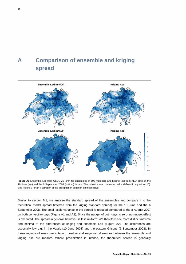
64


A Comparison of ensemble and kriging

spread

Similar to section 6.1, we analyze the standard spread of the ensembles and compare it to the

theoretical model spread (inferred from the kriging standard spread) for the 10 June and the 6

September 2008. The small-scale variance in the spread is reduced compared to the 8 August 2007

on both convective days (Figure A1 and A2). Since the nugget of both days is zero, no nugget effect

is observed. The spread in general, however, is less uniform. We therefore see more distinct maxima

and minima of the differences of kriging and ensemble r.sd (Figure A2). The differences are

especially low e.g. in the Valais (10 June 2008) and the eastern Grisons (6 September 2008). In

these regions of weak precipitation, positive and negative differences between the ensemble and

kriging r.sd are random. Where precipitation is intense, the theoretical spread is generally


Kriging r.sd


Kriging r.sd

Figure A1 Ensemble r.sd from CSCOMB_smn for ensembles of 500 members and kriging r.sd from KED_smn on the

10 June (top) and the 6 September 2008 (bottom) in mm. The robust spread measure r.sd is defined in equation (10).

See Figure 2 for an illustration of the precipitation situation on these days.

65



Appendix

underestimated by the ensembles. An example for this is the red area of strong underestimation in

the Ticino on the 6 September 2008. We suggest these underestimations to be caused by the

skewness of the precipitation distribution. If the very extreme values are coincidentally not realized,

the theoretical spread is underestimated. The lower estimated λs (see Figure 2) of the two convective

days indicate stronger skewness of the precipitation distribution. We therefore expect the described

effect of underestimating the theoretical spread where precipitation is intense to be particularly strong

on the convective days. With a very small ensemble, however, the model spread has a tendency to

be underestimated also on the 8 August 2007. The negative differences in Figure 26 for the

ensemble of 10 members are predominant. The skewness of the precipitation distribution, hence,

seems to have a certain influence on the ensemble size required for a good representation of the

theoretical model spread. On days where a strong transformation has to be applied to the data (i.e.

very skew precipitation distribution and therefore small λs), the spread of the ensembles has a

tendency to underestimate the theoretical spread where precipitation is intense.

B Precipitation fields from conditional

simulation

Best estimates and simulated realizations of precipitation for the combination and the single-sensor

reference method with both station densities are shown in Figure B1 for the 8 August 2007. We find

supported what we discussed in section 6.2 for the 10 June 2008: the simulated ensemble members

represent the spatial variability of precipitation much better than the best estimates. The qualitative

differences from OKGAU to CSGAU and from KED to CSCOMB are yet smaller. As pointed out in

section 4.2.3, we suggest radar to be particularly beneficial in case of convective precipitation. The

radar benefit does not seem to be given in case of the stratiform precipitation occurring on the 8

10 June 2008

6 September 2008

Figure A2 Differences between the ensemble and kriging r.sd for ensembles of 500 members on the 10 June and the 6

September 2008 in mm.

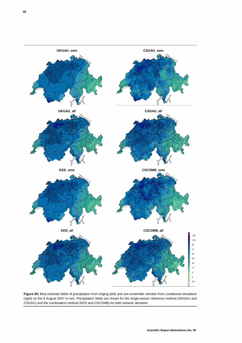
66


OKGAU_smn

CSGAU_smn

OKGAU_all

CSGAU_all

KED_smn

CSCOMB_smn

KED_all

CSCOMB_all

Figure B1 Best estimate fields of precipitation from kriging (left) and one ensemble member from conditional simulation

(right) on the 8 August 2007 in mm. Precipitation fields are shown for the single-sensor reference method (OKGAU and

CSGAU) and the combination method (KED and CSCOMB) for both network densities.

67



Appendix

August 2007. Here, the quality of the additional radar information is low due to large radar errors

(especially in Western Switzerland). This manifests in the particularly low radar coefficient β (see

Figure 2 for a list of estimated βs on the example days). The βs on the example days of convective

precipitation are more than twice as high as the βs on the 8 August 2007. There is thus low trust in

the radar information here and the trend field of the combination, in contrast to the 10 June 2008,

cannot capture the variability in the data. If we compare fields of simulated residuals from

CSCOMB_smn and CSGAU_smn (see Figure B2), we find similar large-scale variation patterns.

Negative residuals are predominantly simulated in the east and the far west, positive residuals in

between. The trend fields of both CSGAU_smn and CSCOMB_smn therefore experience

comparable correction by the simulated residual fields.

On the 8 August 2007, all the precipitation fields from conditional simulation have a lot of small-scale

variance. We again argue with the nugget-to-sill ratio which is between 0.05 and 0.13 for CSCOMB

and CSGAU with both network densities. What can be seen here is the ability of conditional

simulation to represent extreme values. One automatic and three climatological gauges in the

Grisons observe less intense precipitation than the surrounding gauges. Whilst the information of

these gauges does not seem to be reflected in the best estimates, it is represented in the simulated

precipitation fields. The uncertainty with respect to the true field accounted for in the geostatistical

model allows the simulation of very low precipitation amounts.

Would we expect so much small-scale variability in the Swiss Plateau in the case of stratiform

precipitation? Concerning stratiform precipitation, measurement errors at gauges are from

experience relatively small. There are, however, many different factors influencing precipitation. We

could imagine the small-scale variance in the original data to be predominantly caused by gauges

located in mountainous regions, where small lag distances can signify big differences in altitude.

These gauges potentially show a lot of variance, for example caused by orographic forcing

influencing the precipitation amounts. In the case of CSCOMB, this is aggravated by radar problems

in complex terrain. Since we assume the same covariance structure everywhere in the domain

(stationarity assumption), a nugget induced by the gauges situated in mountainous areas will also

cause a lot of small-scale variance in the Swiss Plateau region. This might be in contradiction

CSCOMB_smn

CSGAU_smn

Figure B2 Realizations of the simulated residual field from CSCOMB_smn and CSGAU_smn in transformed space on

the 8 August 2007.

68


OKGAU_smn

CSGAU_smn

OKGAU_all

CSGAU_all

KED_smn

CSCOMB_smn

KED_all

CSCOMB_all

Figure B3 Best estimate fields of precipitation from kriging (left) and one ensemble member from conditional simulation

(right) on the 6 September 2008 in mm. Precipitation fields are shown for the single-sensor reference method (OKGAU

and CSGAU) and the combination method (KED and CSCOMB) for both network densities.

69



Appendix

with the potentially lower variance among the observations in the Swiss Plateau. What we want to

stress here is the fact that assuming the same variogram for the entire domain constitutes a

considerable simplification of the model. We have to bear this simplification in mind when considering

precipitation fields generated with conditional simulation. We should, however, not forget that point

values and not areal averages of precipitation are simulated. This approach can enhance small-scale

variability.

Also on the 6 September 2008, a better representation of local variability of precipitation is achieved

with conditional simulation (Figure B3). Of all the three example days, the 6 September 2008 has the

smallest nugget-to-sill ratios when the dense station network is used and a nugget of zero for both

CSCOMB_smn and CSGAU_smn. The simulated precipitation fields from conditional simulation

therefore have less small-scale variance.

We see the importance of a good sampling for conditional simulation here. With the sparse station

network and without using radar information, only one gauge detects the strong precipitation

maximum in Ticino. The area of this maximum is therefore much smaller in CSGAU_smn than in

CSCOMB or CSGAU_all.

Another interesting issue are the radar artifacts pointing away radially from the Albis radar (we

already highlighted these so called radar stripes in section 4.2.6). They are clearly visible in the radar

composite (see Figure 2), the best estimate field of KED_smn and the trend field (not shown). Also in

the simulated precipitation fields from CSCOMB_smn, the radar stripes are visible. We interpret this

as follows: as can be seen in the radar composite, rain gauge measurements and radar information

are, with the exception of the southern Valais, in accordance with each other. The good agreement of

radar and rain gauge measurements is reflected in the relatively high βs estimated with both station

networks (see Figure 2). Residuals at gauges are therefore small and we would expect the influence

of the simulated residual field to be limited. Thus, adding the simulated residual fields to the trend

cannot remove the radar artifacts present. If we consider the precipitation field from KED_all, we see

that the addition of the climatological gauges made the radar stripes become nearly invisible. Using

all rain gauge observations available, the network is dense enough to correct the radar artifacts

locally. The radar stripes are completely removed in the ensemble members from CSCOMB_all,

where the small-scale variance provides further assistance in removing the radar artifacts.

MeteoSchweiz MeteoSchweiz MeteoSvizzera MétéoSuisse MétéoSuisse

Krähbühlstrasse 58 Flugwetterzentrale Via ai Monti 146 7bis, av. de la Paix Chemin de l'Aérologie

CH-8044 Zürich CH-8060 Zürich-Flughafen CH-6605 Locarno Monti CH-1211 Genève 2 CH-1530 Payerne

T +41 44 256 91 11 T +41 43 816 20 10 T +41 91 756 23 11 T +41 22 716 28 28 T +41 26 662 62 11

www.meteoschweiz.ch www.meteoswiss.ch www.meteosvizzera.ch www.meteosuisse.ch www.meteosuisse.ch

scientific report meteoswiss no. 95 quantifying the ... · meteoswiss for both the automatic rain...

Documents