scitech - microwave passive direction finding
TRANSCRIPT

8/8/2019 SciTech - Microwave Passive Direction Finding
http://slidepdf.com/reader/full/scitech-microwave-passive-direction-finding 1/323

8/8/2019 SciTech - Microwave Passive Direction Finding
http://slidepdf.com/reader/full/scitech-microwave-passive-direction-finding 2/323
This is a corrected reprinting of the 1987 edition originally published by John Wiley & Sons: New York.
All rights reserved. No part of this book m ay be reproduced or used in any form w hatsoever w ithoutwritten permission from the publisher.
Printed in the United States of Am erica
10 9 8 7 6 5 4 3 2 1
ISBN: 1-891121-23-5
SciTech books m ay be purchased at quantity discounts for educational, business, or sales promo tionaluse. For information contact the publisher:
SciTech P ublishing, Inc.5601 N. Haw thorne WayRaleigh, NC 27613(919) 866-1501www.scitechpub.com
Library of Congress Cataloging in Publication Data:Lipsky, Stephen E .
Microwave passive direction finding.
Includes bibliographies and index.1. Radio direction finders. 2. Microwave devices.I. Title.
TK6565.D5L57 1987 621.3841'91 86-33995ISBN 1-891121-23-5
2004 by SciTech Publishing, Inc.Raleigh, NC 27613

8/8/2019 SciTech - Microwave Passive Direction Finding
http://slidepdf.com/reader/full/scitech-microwave-passive-direction-finding 3/323
To two women:
My mother, who always said I couldMy wife, HyIa, who knew I should

8/8/2019 SciTech - Microwave Passive Direction Finding
http://slidepdf.com/reader/full/scitech-microwave-passive-direction-finding 4/323
Foreword
At long last a very professional, complete, and carefully unified consolidation ofthe latest techniques, both systems and components, is available on the subject ofmicrowave passive direction finding. This volume brings together, for the first time,the latest work done in microwave direction finding by individuals and groupsdispersed w orldwide. This field is in a period of dynamic innovative growth, spurredby the growing availability of higher-speed lower-cost digital processing circuitry.This book is a welcome and needed assistance to direction finder designers.
L E O N R I EB M A N , P H . D .

8/8/2019 SciTech - Microwave Passive Direction Finding
http://slidepdf.com/reader/full/scitech-microwave-passive-direction-finding 5/323
Preface to theSciTech Edition
The present nature of modern electronic warfare dictates the use of passive detec-tion and direction finding of microwave threats. The use of active radar by thesource signal unfortunately prompts missile defensive countermeasures and otherdestructive means. Threat radars, therefore, cannot be allowed to transmit a contin-uous signal for fear of homing devices. Similarly, threat location radars, if used byreceiving source, cannot be used for the same reason.Passive detection, on theother hand, permits the determination of the direction-of-arrival of a radar signalbased on monopulse reception of just one or a few pulses. Pulse digital processingcan then augment this detection by comparing the characteristics of received pulseto a previously stored da tabase of threats, thus identifying the threat types.
This book describes methods of measurements of the pulse directionwithoutthe knowledge of the RF frequency. This permits a wide-open m onopulse receiverfor surveillance of unknow n environments for immediate threat detection and warn-ing. The various configurations of passive DF receivers are explained and analyzed.Both radar warning systems (RWR) and ship defense (SD) systems are thoroughlyexplained by photographs and block diagrams. The mathematics of DF determina-tion including accuracy, signal-to-noise, and intercept-probability, are fully covered
in detail. The book provides a primer of the theory and implementation of currentequipment, and offers much information not available in any other single source.The first edition was used in teaching graduate courses in microwave receivers
at Drexel and other universities. It is hoped that the availability of this SciTech edi-tion will further the study of the DF art.
July 4, 2003Stephen E. Lipsky, Ph.D.

8/8/2019 SciTech - Microwave Passive Direction Finding
http://slidepdf.com/reader/full/scitech-microwave-passive-direction-finding 6/323
Preface
This book compiles the many methods of microwave passive direction finding intoa single technology, identifiable as such. I have attempted to present the results of
the many systems designs and concepts that have evolved early radar directionfinding (DF) into a specialized science and state the unique sets of rules andprinciples that codify microwave passive DF technology.
My method of presentation is tutorial and leads the reader through DF theory inan understandable manner, utilizing mathematics where necessary to understandthe concepts and to provide direct design answers. I have found from my experiencein writing papers and giving presentations, that most engineers want to be able toreach definitive conclusions based on clear paths of reasoning. To accomplish this,I have described DF technology in theory, by comparison, mathematical analysis,and reference. Where complex questions are to be answered, I have given practicalexamples. Where many competing factors must be considered, as in the case ofthe sensitivity of a system for a given accuracy and false-alarm rate, I have madeextensive use of computer-developed graphs to simplify the design process. Toreinforce this approach, numerous block diagrams, alternate design methods, andillustrations are used.
This volume has been oriented to both the student and practicing microwaveengineer. It is presupposed that the reader is familiar with complex variables, somestatistics, fields and wave theory, and has a tutorial understanding of radar andgeneral microwave methods. Based on this background, the concept of directionfinding is introduced in Chapter 1 as an outgrowth of radar and high-frequencydirection finding methods prior to and after World War II. Usage and requirementsare stated to show the reasons for the separation of DF technology from its radarorigins. Chapter 2 traces the development of monopulse receiver lobing as a naturalsolution to problems in scanning radar and associated direction finding methods.The postulates and class definitions of monopulse are defined with examples of

8/8/2019 SciTech - Microwave Passive Direction Finding
http://slidepdf.com/reader/full/scitech-microwave-passive-direction-finding 7/323
processing techniques. DF by receiver antenna pattern comparison, introduced inthis chapter, is extensively amplified in Chapter 3 by analysis of the many typesof antenna elements that achieve required DF phase and amplitude characteristics.Much attention is directed to spiral antenna technology, including multimode operationand extension into the millimeter frequency range. Horn, reflector, and mode-feeddeveloped pattern antennas, such as the Honey-Jones, are presented in variousconfigurations.
Chapter 4 blocks out practical implementations of receivers and processors capableof extracting the DF information from the received signals. Block diagrams of radarwarning and ELIN T DF systems are used to give the reader a foundation of practicaltechnology. Here may be found descriptions of the unusual: subcommutation, su-percommutation, monochannel phase-encoding, and the more commonly knownmonopulse techniques. Various configurations of "frontends" and receivers usedfor RWR and ELINT receivers are explained with diagrams of amplitude, phase,and sum-and-difference processors. The three classes of monopulse processors aredescribed with their broadband variants, the detector-log-video-amplifier and thewide bandwidth phase discriminator (correlator). Chapters 5 and 6 cover arraytechnology as applied to receivers. Parallel beam arrays, such as the Butler planar,moded circular, and switched type, are discussed, with examples given of each.
Rotman-Turner and R-KR lens-fed arrays are presented to illustrate parallel beamtime summation processes that are in common use. Movable reflector, beam, andswitched multielement beam-scanning arrays are also described. Interferometer DFsystems, which are becoming most important now due to their capability for higherDF accuracy, are detailed in Chapter 5, with practical design equations.
Analytical approaches to the design and analysis of the various receiver typesused in passive direction finding are presented in Chapters 7-9. They are intendedto define the mathematical aspects of receiver technology in an understandable yet
detailed manner that will reward the reader with a comprehensive grasp of someobtuse concepts. Chapter 7 develops methods for signal detection, describing thegain and noise-limited crystal video receiver, the superheterodyne receiver, anddownconverter variations of both. Signal-to-noise relationships for pre- and post-detection are derived. Curves permitting determination of signal-to-noise output forsignal-to-noise input for various laws of detection are drawn, permitting determinationof the sensitivity of a given design . This is done not jus t for the tangential sensitivitycase but for the entire dynamic range of detection using derivations not readily
found in the literature. Chapter 8 concentrates on probability-of-detection and false-alarm rates for both the well-established envelope (superheterodyne) and wide-bandquadratic (crystal video) receivers. Here again graphical methods are used specificallyto relate to the problems of searching for a signal of unknown parameters with areceiver that has characteristics that may only approximate those needed for detectionof the intercept's RF and pulse characteristics. Chapter 9, devoted to determiningthe accuracy of a DF system for amplitude and phase monopulse configurations,is an outgrowth of many articles and papers on this subject. Error budget andchannel balance considerations are derived and presented in mathematical and graphi-cal form, with examples of the method of calculation. The effects of noise on

8/8/2019 SciTech - Microwave Passive Direction Finding
http://slidepdf.com/reader/full/scitech-microwave-passive-direction-finding 8/323
accuracy are derived in readily understandable terms, permitting determination ofactual operating characteristics of system designs. Practical installation questionsare addressed, and recommendations for achieving optimum results are discussed.
Signal analog and digital processing and display methods are examined in Chapter10, starting with a basic description of three types of logarithmic amplifier designsfor real- and non-real-time signal processing, followed by a description of signalprocessing and concluding with displays and display configurations. The methodologyof pulse-on-pulse operation to reduce receiver "shadow" or dead time is describedwith circuit configurations of practical designs. Wide bandwidth amplitude andphase measurement methods are also analyzed. Complete reference to source ma-terial is included throughout the book for further study and investigation.
I have tried to convey my understanding of microwave passive direction findingin a readable form that will encourage technical curiosity and provide the satisfactionthat comes with a positive understanding of why this technology is an art.
STEPHEN E. LIPSKYRydal, PennsylvaniaMay 1987
8/8/2019 SciTech - Microwave Passive Direction Finding
http://slidepdf.com/reader/full/scitech-microwave-passive-direction-finding 9/323
Acknowledgments
In any book of this type, it is hard to claim originality since most of the conceptsand ideas are the work of many teams of engineers working at many differentcompanies. I therefore wish to thank my associates at American Electronic Laboratories,Inc., the General Instrument Corporation, Polarad Electronics, and the Loral Cor-poration for the opportunity to learn the technology. I am especially appreciativeof the support of Dr. Leon R iebman, the Chairman of the Board, and Mark R onald,president of AEL Industries, Inc., for their faith in and support of this endeavor.I also wish to thank my other AEL associates, in particular, Dr. Baruch Even-Orfor his essential assistance and help in Chapters 7,8, and 9, especially with regardto the derivations and computer plots, and Walter Bohlman, John Bail, and BobKopski for their review and suggestions. Additional thanks go to Ernie Buono, JoeGiusti, and the AEL ILS Division for their development of the illustrations,photos, and layouts.
I would like to acknowledge the assistance of Richard Stroh and Stig Rehnmarkof Anaren, George Monser of the Raytheon Company, Ron Hirsch of RHG, andRichard Hollis of Watkins Johnson. I appreciate the help and guidance of otherrespected associates such as Jim Adams of the General Instrument Corporation and
Lloyd Robinson at the Stanford Research Institute. I am indebted to Amos Shahamof Elisra, Bene Baraq, Israel, for his descriptions, and to Dr. Donald Linden ofthe Dalmo Victor Division of the Singer Corporation. The release of technical data,descriptive material photos, and illustrations by the above and many other contrib-utors have made this book possible. I also wish to thank Mr. George Telecki, myeditor at Wiley, for his faith, encouragement, and patience.

8/8/2019 SciTech - Microwave Passive Direction Finding
http://slidepdf.com/reader/full/scitech-microwave-passive-direction-finding 10/323
Last but far from least, I wish to thank Judith Butterfield for her help, unendingpatience, and diligence in the preparation of this manuscript. In any endeavor ofthis sort no one is alone. I thank my wife, HyIa, for her encouragement andforbearance, without which this book would have neither been started nor com-pleted.
STEPHEN E. LIPSKY

8/8/2019 SciTech - Microwave Passive Direction Finding
http://slidepdf.com/reader/full/scitech-microwave-passive-direction-finding 11/323
xvThis page has been reformatted by Knovel to provide easier navigation.
Contents
Foreword ............................................................................. vii
Preface to the SciTech Edition ............................................ viii
Preface ................................................................................ ix
Acknowledgments ............................................................... xiii
1. Evolution and Uses of Passive DirectionFinding ......................................................................... 1
1.1 Evolution .......................................................................... 2
1.2 HF DF Origins ................................................................. 3
1.3 Radar DF Origins ............................................................ 6
1.4 Uses of Passive DF ......................................................... 81.5 Summary and Guide to the Book ................................... 11
References ............................................................................... 11
2. DF Receiver Theory .................................................... 12
2.1 Evolution of Rotating DF Systems .................................. 12
2.2 Concept of Monopulse .................................................... 24
2.3 Monopulse Angle Determination ..................................... 29
2.4 Birth of Passive Direction FindingTechniques ...................................................................... 34
2.5 Summary ......................................................................... 34
References ............................................................................... 35

8/8/2019 SciTech - Microwave Passive Direction Finding
http://slidepdf.com/reader/full/scitech-microwave-passive-direction-finding 12/323
xvi Contents
This page has been reformatted by Knovel to provide easier navigation.
3. Antenna Elements for Microwave PassiveDirection Finding ........................................................ 36
3.1 Terminology and Conventions ........................................ 36
3.2 Spiral Antennas ............................................................... 39 3.3 Horn Antennas ................................................................ 68
3.4 Multimode DF Horn Antennas ........................................ 79
3.5 Rotating Reflector Antennas ........................................... 92
3.6 Summary ......................................................................... 98
References ............................................................................... 99
4. DF Receiver Configurations ....................................... 101
4.1 DF Radar Warning Receivers ......................................... 101
4.2 Phase and Sum and Difference Monopulse DFReceivers ........................................................................ 107
4.3 Subcommutation Methods .............................................. 111 4.4 Supercommutation .......................................................... 116
4.5 Monochannel Monopulse ................................................ 119
4.6 Parallel DF Channelization ............................................. 122
4.7 Multibeam DF Arrays ...................................................... 123
4.8 Summary ......................................................................... 124
References ............................................................................... 125
5. DF Antenna Arrays ..................................................... 126
5.1 Passive Detection Arrays ................................................ 128
5.2 Parallel Beam Formed Arrays ......................................... 129
5.3 Planar Butler Array .......................................................... 130
5.4 Circular Butler-Fed Array ................................................ 132
5.5 Lens-Fed Arrays .............................................................. 138
5.6 Parallel Beam Septum Antenna ...................................... 147
5.7 Switched-Beam Arrays ................................................... 150
5.8 Summary ......................................................................... 152
References ............................................................................... 154

8/8/2019 SciTech - Microwave Passive Direction Finding
http://slidepdf.com/reader/full/scitech-microwave-passive-direction-finding 13/323
Contents xvii
This page has been reformatted by Knovel to provide easier navigation.
6. Interferometer DF Techniques ................................... 155
6.1 Mathematics of Interferometry ........................................ 156
6.2 Solution of the Interferometer Equations ........................ 163
6.3 Multiple Aperture Systems .............................................. 165
6.4 Linear and Circular Interferometer Arrays ...................... 167
6.5 Circular Interferometer Systems ..................................... 168
6.6 Summary ......................................................................... 170
References ............................................................................... 170
7. Methods for Signal Detection .................................... 171
7.1 Crystal Video Receiver ................................................... 172
7.2 Superheterodyne Receiver ............................................. 191
7.3 Downconverier Receiver ................................................. 203
References ............................................................................... 205
8. Probability of Detection ............................................. 207
8.1 False Alarm Probability ................................................... 208
8.2 Probability of Signal Detection in Noise .......................... 213
8.3 Intercept Probability ........................................................ 223
8.4 Window Function Probability Concept ............................ 229
8.5 Summary ......................................................................... 231
References ............................................................................... 231
9. Accuracy of DF Systems ............................................ 233
9.1 Antenna Accuracy for MultibeamSystems ........................................................................... 234
9.2 Noise Accuracy of Amplitude Comparison DFSystems ........................................................................... 248
9.3 Noise Accuracy in Phase Measurement DFSystems ........................................................................... 252
9.4 Accuracy as a Function of Installation ............................ 256
References ............................................................................... 262

8/8/2019 SciTech - Microwave Passive Direction Finding
http://slidepdf.com/reader/full/scitech-microwave-passive-direction-finding 14/323

8/8/2019 SciTech - Microwave Passive Direction Finding
http://slidepdf.com/reader/full/scitech-microwave-passive-direction-finding 15/323
Evolution and Usesof Passive
Direction Finding
In recent years, microwave passive direction finding (DF) has emerged as a distinct
technology apart from HF/YH F and radar associated D F methods. This has occurredas the result of many factors, the most important being recognition of electronicwarfare as an art. In the post-W orld W ar II period , radar-controlled weapon systemshave undergone extensive development aided, in no small part, by the enormousworldwide investments and subsequent achievements in avionics, semiconductor,and radar technologies. In the initial stages of this expansion, the use of directionfinding, both active and passive, was part of the more general task of gatheringelectronic battlefield intelligence (ELINT). At first, the recognition of the number
and types of hostile emitters, in a field of many signals, was accomplished by lowprobability-of-intercept systems, typically using rotating antennas, narrow bandwidthscanning receivers, and real-time pulse processing and display techniques. Thismethodology was consistent with speed of the available data-handling processes ofthat time and the human operator's ability to make use of the information.
More recently, w ith the advent of sophisticated high-performance antiaircraftand antiship missile systems, electronic warfare has been tasked with the problemof recognizing not just the threat but rather the state it is in: acquisition, launch,
and control or terminal guidance. The need for early warning and protection forships , high-speed aircraft, and ground forces has led to the development of complexelectronic warfare protection suites and a class of equipment known as radar warningreceivers (RWR), both of which make extensive use of microwave passive DFmethods. Reaction time has also become a forcing function since there may be onlyminutes or seconds between detection and destruction, often requiring that a decisionbe made automatically without a human operator. To make matters more complex,the proliferation of equipment sold, captured, and exchanged between hostile coun-
tries, formally friendly to each other, has all but destroyed recognition of the radarequipment of a friend or a foe on a "country developed" type basis.
Chapter One
8/8/2019 SciTech - Microwave Passive Direction Finding
http://slidepdf.com/reader/full/scitech-microwave-passive-direction-finding 16/323
The answer to this current situation has been the development of real-timeelectronic warfare techniques utilizing high probability-of-intercept computer-con-trolled systems to sort out the environment on a pulse-by-pulse basis over wide-frequency band widths and full 360 degree azimuthal fields-of-view. The signaldensity and quantity of data obtained by high-probability intercept receivers had,in the past, completely outstripped the then available processing capabilities. For-tunately, the same technology that has exacerbated the threat determination problemhas improved digital capacity by providing more storage in smaller volumes andat faster throughput rates, making recognition and sorting of signals on a pulse-by-pulse basis now practical. In the microwave radio frequency (RF) area, perfectionof wide bandwidth instantaneous frequency measurement has added an additionalimpetus to the need for instantaneous intercept DF data since both frequency andDF information can be obtained on a single pulse basis and used as presorting too ls,using one to direct the other to reduce system processor workloads.
Improvements in antennas and the availability of matched microwave solid-stateRF amplifiers now permit greater ranges of detection and higher accuracies to beobtained over wider instantaneous band widths and at higher sensitivities. Theseadvances have made microwave passive DF technology self-adaptive as comparedto active HF and microwave radar systems that were greatly aided by a priori
knowledge of frequency, anticipated direction, or pulse characteristics of a knownilluminating transmitted signal. Passive direction finding has emerged as a stand-alone technology completely adaptive to complex unknown environments and fullycapable of operating with the multitudinous types of signals found in modern electronicwarfare.
1 .1 EVOLUTION
This book has been written in recognition of the development of microwave passivedirection finding as a basic technology permitting one to develop a synergistic viewof the many concepts to permit the selection of the technique that best fits theproblem to be solved. The material to be covered has been selected from a verywide range of published, known, and new techniques that meet an essentialrule— that of practical application. There are many DF methods based upon theoreticalprojections of performance, idealized antenna characteristics, computer assets, and
so on, that remained submerged in the world of useful technology. In no other fieldperhaps have there been as many false starts, aborted designs, and abandonedsystems due perhaps to the reactive method by which electronic warfare equipmenthas evolved. The appearance of a threat is countered by a threat recognition systemuntil the next threat is discovered. A major factor in the process is the constantneed to improve the probability of receiving few pulses on short signal bursts sinceradiation security dictates that radar and target determination systems minimize on-the-air time. Passive detection systems have therefore been designed to meet thischallenge. The high density of signals has mandated computer sorting and controlas a necessity.

8/8/2019 SciTech - Microwave Passive Direction Finding
http://slidepdf.com/reader/full/scitech-microwave-passive-direction-finding 17/323
Passive direction finding has also emerged for weapon targeting . As the accuracyof DF systems improves (2 degrees root mean square (RMS) accuracy seems to bethe magic accuracy number), missiles and aircraft can use the passive DF data tosteer along the line-of-bearing to intercept targets, using terminal guidance m ethodsfor high accuracy at the last stage. The technology of microwave direction findingis undergoing constant pressure to increase DF accuracy for this purpose.
This book will present the development of passive DF from its early origins topresent-day methods to include monopulse, beam-formed arrays, interferometers,and rotating antenna systems. Operation of important subsystems that affect overallperformance will be analyzed, with mathematical models presented for key factors.Determination of signal-to-noise ratios, detector operation, monopulse ratio nor-malization, DF accuracy, and intercept probability will be detailed to give a synergisticunderstanding of the system aspects of the solution.
1.2 HF DF OR IGINS
Passive direction finding was the first type of target location system based uponradio techniques. The major advances in this art were derived from the needs of
both world wars. It is interesting to note that much of the technique developmentand patent protection w as filed in the 19 20 -19 40 time pe riod, w hen direction findingwas concentrated in the "shortwave" or 0.5-30 MHz frequency range. Initial conceptsrecognized that the nonisotropic or directional pattern characteristic response of oneor more antennas could be used to determine the direction-of-arrival of a signal bynoting the pointing position of the receiver's "imperfect" antenna when the receivedamplitude peaked or nulled as the antenna was rotated. Emitter location by triangu-lation, the intersection of three or more bearing lines, required more sophisticated
directional antennas and new methods to achieve improved bearing accuracy. For-tunately, most signals remained on the air long enough to permit multiple bearingmeasurements to be made, either by a single receiver moved to different locationsor by several geographically dispersed receivers tuned to the same frequency and,it was hoped, to the same signal. Continuing needs for better accuracy soon led toantennas with better perform ance, that is , more signal change per degree of rotation.Null type systems, such as the loop antenna and multiple element arrays, permittedremarkable accuracies to be achieved, in some cases to the extent of the limit of
errors due to summation of the ground and sky wave propagation paths. This latterlimitation in the HF range turned out to be a major problem. The sky wave or"skip" component arrived randomly polarized causing serious null precession orshift when added to the well-behaved vertically polarized ground wave signal.
Adcock (1), working in England in 1919, patented a narrow-aperture (shortenedlength) array of four orthogonally located elements, which, when summed andcompared, could give the effect of two crossed figure-eight patterns as shown inFigure 1-1. Comparisons of the signals provided DF field patterns that had a 180degree ambiguity, which was resolved by comparison to the sum of all of theantenna patterns, which was omnidirectional. Sometimes the signal from another

8/8/2019 SciTech - Microwave Passive Direction Finding
http://slidepdf.com/reader/full/scitech-microwave-passive-direction-finding 18/323
Angle of arrival
Antennas
Display
Receivers
a) System of four monopoles
Figure 1-1. Adcock antenna and resulting patterns,(a ) System of four monopoles. (b ) Display ofpatterns of (a).
b) Display patterns of a)
E-W-S
N E
RW
R R
S
R

8/8/2019 SciTech - Microwave Passive Direction Finding
http://slidepdf.com/reader/full/scitech-microwave-passive-direction-finding 19/323
element, called a sense antenna, would be used to provide a pattern that wouldgive a cardioid, or single-null response. This technique was also used with loopantennas for the same ambiguity resolution purpose. The German Wullenweberarray and others improved matters by using longer medium- and wide-aperturearrays of as many as 36 elements dispersed around a large diameter circle. A setof one third of the antenna elements was passed through a capacitively coupledrotating joint through an RF delay line and summed in two groups of four elementseach, as shown in Figure 1-2. The two groups were subtracted with the resultantbeing a null (Fig. l-2b) that physically rotated at the mechanical rotational rate ofthe mechanism, known as a goniometer. When connected to a suitable receiver,DF measurements could be made to fractional degree accuracy, as limited above(see Ref. 2).
During the period from World War II to the present, the Adcock and similarantenna systems were improved. It is worth noting, for future reference to microwavedes igns , that the improvem ents to these systems moved in the direction of developing
Capacitor rotor platesDspersed set ofantenna eements
Capacitor stator plates
Sum network (2) Sum network (Z)
Dfference network (A)
Rotor
(a) Configuration
tb) D*-Y
Pattern
Figure 1-2. A goniometer rotating capacitor transformer used to develop a rotating null for DF determination.

8/8/2019 SciTech - Microwave Passive Direction Finding
http://slidepdf.com/reader/full/scitech-microwave-passive-direction-finding 20/323
both the difference and the sum patterns of grouped elements and a means ofcomparing the two simultaneously to remove common signal amplitude variations,a technique that we shall see is similar to radar "monopulse" methods.
1.3 RADARDFORIGINS
Direction finding in the microwave frequency range, defined loosely here as 500-100,000 M Hz, derived from two sources: the HF direction finding systems describedabove and the invention of radar, the technique of radio ranging and directionfinding. Transition of operating techniques from the HF to the microwave regionwas readily accomplished since greater aperture or wave interception area for theantennas could be obtained because microwave wavelengths were smaller at thehigher operating microwave frequencies. Propagation of microwave energy was byline-of-sight, not by reflection from the ionosphere due to the higher frequenciesinvolved, fortunately eliminating multipath "skip" problems.
Radar development was rapidly advanced during the late 1930s in Germany,England, and the United States in anticipation of World War II. Stories about theuse of radar in the battle of Britain are legend as are some of the radar countermea-
sures developed as a necessity. This book will not attempt to document each stepbut will rather identify the key factors leading to the present concept of passivedirection finding as applied to electronic warfare.
Early radars were generally m onostatic (collocated transmitter and receiver) usingthe same antenna system to transmit and receive a series of pulsed signals. Shortpulse signals allowed high peak powers to be transmitted for maximum range. Theinterval between the pulses (the pulse repetition interval PRI) was chosen to provideunambiguous range returns. The time difference between the transmitted signal and
the receipt of the target echo was measured to extract range information. To obtainangle information, the antenna was rotated through a know n angle to cover a desiredazimuthal sector, and the pointing direction at which the radar return was receivedwas noted. Tactical needs to increase range measurement led to the developmentof higher power transmitters, high gain, more efficient antennas, and better angle-of-arrival techniques. As components improved it was possible to make advancesin peak power generation by shortening the transmitted pulse widths. DF resolutionwas improved by the use of higher frequency narrow beamwidth antennas. This
required better scanning methods and the development of scanning or sequentiallobing antenna feeds to track or follow a specific target for gun aiming purposesor to present a polar map of all signals (plan position indication (PPI)).
New requirements called for the radar to view a sector in azimuth broadly whilesimultaneously moving or scanning the antenna feed slightly in a periodic fashionto "paint" across, or modulate, the target (called nutating), illuminating it at aknown rate or scan . If the radar return scan illumination w as equal to the transm itterscan illumination as determined by comparing the phase and amplitude of the scanmodulation of the return to that of the transmitted signal, the radar was deemed tobe on "boresight." If the return scan modulations were unequal, an error signal was

8/8/2019 SciTech - Microwave Passive Direction Finding
http://slidepdf.com/reader/full/scitech-microwave-passive-direction-finding 21/323
developed and negatively fed back to the antenna servo, or positioning system, toeffect a correction. By scanning in either a circular or conical mode, it was possibleto develop both azimuth and elevation correction signals, allowing for full trackingor "track-while-scan" operation. Sequential transmitter lobing accomplished thesame effect as nutation by switching between two squinted or physically displacedtransmit beams at a prescribed rate. In both of these cases the scan modulation wascontained in the transmitted beam , and the symmetry and amplitude of the illuminatingbeam could be detected at thetarget to indicate a "track" or "lock-on" condition.The symmetry of the received scan at the radar was a measure of nearness toboresight of the radar. A reduction of the amplitude of the scan would induce theuse of more radar system gain to "tighten" or better lock the radar's antenna aimingservo.
Early in the development of radar certain problems of resolution error becameevident. In a sequential or scanning radar the received signal consisted of a seriesof pulses, differing in amplitude by the scan rate. If there was any pulse-to-pulsevariation not due to the intended scan, there were errors. This happened as a resultof target movement or scintillation. Angular jitter due to multiple reflections in thepath of the illuminating beam caused substantial variations. While range gating,which is the process of turning the radar receiver on only over the time period
corresponding to the anticipated range of the expected return, helped this problem,another method was needed. A new DF measurement technique was developed toform and detect the received beam by simultaneously receiving it in two separatedbut collocated receiver an tenna lobes. The pulse-by-pulse ratio of the received pulsesin each beam would then contain all of the DF information, independently of anypulse amplitude variation. The approach was aptly named monopulse. There is animportant difference in this technique in comparison to scanning pulse radars: Withmonopulse radars the transmitter emits a constant amplitude signal, with DF information
being extracted from the ratio of the pulse amplitudes (or phases) of two or morereceiver beams that are angularly (or phase) offset in a known manner while beingphysically scanned. The DF lobing or scanning is not contained in the transmitbeam as before. Since this technique, known as passive lobing, can be done on asingle pulse, DF measurements can be made on target-reflected pulses containingintrapulse variations, since it is theratio of the two receiver beams that holds theDF data. This ratio, as will be shown, normalizes the intercept return removing allintrapulse or common-mode variation, resulting in a very basic improvement.
The art of passive DF determination was an outgrowth of the development ofmonopulse radar. The transmit beam was only used to illuminate the target; all DFmeasurements were made by the receiver. Since the receiver, monopulse antennaor array was corotated and pointed with the transmitter antenna (called monostatic),the radar system had an advance idea of where the target would be by knowing theaiming direction of the antenna system. As receiver sensitivities improved, it oftenbecame convenient to separate the transmit antenna from the monopulse receiversystem and not collocate the two, leading to the development of the separated (orbistatic) radar where the transm itter "illumina ted" the target from one location whilethe receiver detected the angle of arrival of the return from another. By further

8/8/2019 SciTech - Microwave Passive Direction Finding
http://slidepdf.com/reader/full/scitech-microwave-passive-direction-finding 22/323
improving the receiver sensitivities and associated antenna system, signals normallytransmitted by the target, such as its own radar, could be used as the returns,eliminating the need for the "illumination" transmitter altogether. Under these con-ditions, no emissions took place at the receive point, the DF technique was termed"passive," and the art of passive direction finding was born. It is this part of theoverall radar technology that will be examined in detail in this book.
1.4 USESOFPASSIVEDF
Some of the more important uses of microwave passive direction finding relate tomodern electronic warfare applications. It is relevant to discuss some of the moresignificant ones.
Early Warning Threat Detection. Early warning signal or threat detection isperhaps the chief use of passive DF. With high-speed processing it is possible todetect and identify a threat in a dense environment by determining the status of thethreat amplitude, scan, pulse width, and period modulation. From this informationit is possible to recognize the presence of an imminent attack and permit counter-
measures to be taken. One of the first uses of passive direction finding was to locatethe positions of ships and submarines by shore stations and by the submarinesthemselves to protect against antisubmarine patrols. In World War II this was animportant activity. Allied DF methods were well advanced due in part to the rescueof an IT&T DF research group from France just before the fall of Paris (3).
German submarines, in the latter part of the war, were equipped with microwavereceivers and crystal detectors, operating at L-band radar frequencies, to give earlywarning of British antisubmarine radars. M ost of these systems, primative by today's
standards, were hand directed and limited by the sensitivities obtainable. Crystaldiode video receivers, with sensitivities of only - 4 5 dBm (decibels below onemilliwatt of received power in 50 ohms) sensitivity and some antenna gain, gavesuitable warning in many cases, however, since a radar signal travels to the targetand back, suffering double attenuation in addition to the target reflection or returnloss. This m ade the radar signal considerably stronger at the target than at the radar,requiring less target receiver sensitivity. As a result, British RAF L-band shoreradars used to detect submarines were detected themselves by the submarines at
ranges beyond that of the radar, giving them time to escape. It was only when theBritish moved their radars toS-band and the Germans were unable to detect themwere the tables turned (4). The principle still prevails for radar warning receiverswhere simple crystal video detectors are often used to provide detection at approximatelytwice the radar's detection range.
Early line-of-sight aircraft DF systems were relatively successful since the higheraltitude of a plane could give warning out to the radar horizon if receiver sensitivitieswere sufficient. Much of this early effort has been well documented in Ref. 5. Theproblem of detecting the scanning victim radar with a rotating DF receive antennawas severe since the detection probabilities resulting from two rotations—that of

8/8/2019 SciTech - Microwave Passive Direction Finding
http://slidepdf.com/reader/full/scitech-microwave-passive-direction-finding 23/323
the receiver and that of the radar (numbers less than 1)—multiply. The need forsensitivities high enough to receive the backlobes of the radar antennas, which wereabout 30 dB below the beam peak, was finally achieved, partially removing theeffects of the radar antenna rotation. This increased the dynamic range of receiveroperation, necessitating the development of compressive or "logarithmic" ampli-fiers, which became a key factor in the development of monopulse technology.
Targeting, Homing, and Jamming. In modern warfare, missiles are usuallylaunched in the general direction of the target by a radar system that acquires thetarget, feeds initial coordinates to the missile prior to launch, and then continuesto transmit guidance signals to the missile along its way. The missile system acquisitionand guidance radar revealsitself, however, by the need to radiate energy. A passiveDF system can be used as an "antiradiation" technique for DF steering to a targetradar. For targets that shut off their radars to prevent detection, passive DF canbring the missile to a range near the target before it shuts down, after which aself-
contained term inal guidance missile-borne radar can be activated to guide the missileto hit the target before countermeasure action can be taken. The relative physicalsmall size of a missile necessitates the use of correspondingly small size on-boardantennas operating at higher frequencies to reduce wavelength-associated dimensions.
These concepts have prompted the development of small high-accuracy passive D Fsystems.Repeater type jammers are concerned with generating a deceptive return signal
at high power on the true target return, usually within the backporch of the illuminatingpulse. This is done to modulate the echo scan falsely, causing loss of lock at theradar. To accomplish this, it is necessary to build retrodirective DF systems withhigh angular accuracy for both receiving and transmitting antennas, since narrowerantenna beamwidths used to give better antenna gain require that the antenna be
pointed precisely. As a result, more accurate DF system s, depending upon arrayingor combining of many antennas, are used to obtain larger apertures for higherangular resolution, rather than depending on the pattern accuracy of individual DFantennas. This new technology makes use of lens-fed or switched-phaseshift arraysto form and steer narrow beam s and is a factor in the development of DF technologyapart from radar.
Electronic Intelligence. Electronic Intelligence (ELINT) is an important use of
passive direction finding since, because no energy is radiated, passive DF can beused discretely to calibrate the electromagnetic spectrum continuously. In wartimeELINT determines the electronic order of battle (EOB); in peacetime it is the dailyactivity of updating or mapping the environment for the purposes of detecting newsignals and changes of deployment of threats or forces, as well as providing ageneral measure of radio and radar traffic. A radar transmitter, for example, emitsa signal that identifies itself in many w ays. RF frequency, pulse width, pulse interval,and signal grouping provides real-time descriptors that can identify the type of radarin use. Scan or lack of it, scan frequency, and received power add additionalinformation. Indeed, in electronic intelligence applications, it is possible to codify

8/8/2019 SciTech - Microwave Passive Direction Finding
http://slidepdf.com/reader/full/scitech-microwave-passive-direction-finding 24/323
types, classes, and names of radars based upon observation of these parametersand to use this information as a "telephone directory" or "look-up" table whenidentification is needed. Radar is active; it reveals itself and in so doing providesa means to be countered.
The relative lack of published theory and information about passive directionfinding derives from its counterpurpose to radar and other signals. In general, passivedirection finding adds the missing dimensions to defensive electronic warfare,determination of the angle-of-arrival, and identification and subsequent location ofradiating signals without revealing DF receiver presence or operating technique.Passive DF is useful in quiescent peacetime situations to calibrate a signal environ-ment by determining location of known signals. It is essential in wartime to providerecognition of the signals and defense against radar and other RF directed threatseither by warning of their presence or by steering a jamming signal, missile, ordispensing countermeasures. With these objectives, passive direction finding alwaysstrives for maximum accuracy in the least possible time as a primary consideration.Performance tradeoffs must naturally be made in both cost and installation; however,the methods and technology of passive direction finding provide a challengingcontrast to the well-known and accepted technology of radar.
Data Reduction. Despite the improvements cited earlier, digital data rates arestill the limiting factor to better DF processing. There are simply too many signalsto process at one time. The "down" or "shadow" time of an electronic supportmeasure (ESM) system, can be improved by waning or thinning the environmentby true angle-of-arrival using frequency as presorting descriptors to limit data flow.Although this approach can make a system blind at times, the actual refresh orupdate rate of an operator-assisted ESM system can be dramatically improved. Toobtain these desired results, it becomes important to improve accuracy. Consider
a received radar intercept: As the radar scans, each pulse varies in signal strengthfrom its predecessor throughout the transmitter's antenna beamwidth. This causeseach pulse to be received at a different signal-to-noise ratio by the passive DFsystem. In simultaneous amplitude comparison DF receivers, the DF determinationrules can change unless signal strength is well above a preset threshold. If care isnot taken, a single signal can appear as a multitude of signals differing in manycharacteristics, as the signal-to-noise ratio varies causing errors, and making signalseparation extremely difficult. The solution for this is averaging or adding processing
gain to compensate; however, this takes time. The problem may be tolerable forELINT but intolerable for threat warning.
The availability of instantaneous frequency information can also be used to sortsignals quite accurately and in some instances can correct for any known bearingversus frequency anomalies that are repeatable. This latter feature is especiallyuseful for aircraft that can be calibrated under anechoic conditions. Digital look-up tables can also be used to extend the range of frequency ambiguous systems,such as interferometers, by recognizing that null shifts, for example, will occur atcertain frequencies that are half-wavelength multiples.

8/8/2019 SciTech - Microwave Passive Direction Finding
http://slidepdf.com/reader/full/scitech-microwave-passive-direction-finding 25/323
1.5 SUMMARY AND GUIDE TO THE BOOK
This first chapter has introduced the concept of microw ave passive direction findingas a science apart from radar receivers, the purpose being to permit a synergisticexamination of the theory, antennas, and techniques that constitute the technology.The roots of modern passive direction finding evolved from early HF/VHF andradar methods. Solutions, found to solve radar problems, have been used to moldpassive direction finding into a more sophisticated unified art, which, in combinationwith digital methods, has made this technique a key factor in present-day electronicwarfare systems.
The remainder of the book has been divided topically. Chapter 2 develops DFreceiver theory and the concepts of monopulse. Chapter 3 details antennas for DFapplications, describing operation modes, theory of operation, and key details ofdesign. Chapter 4 shows how various receivers can be configured to extract the DFdata optimally. The important concepts of receiver antenna arrays are explained inChapter 5. Interferometer antennas, a special form of arrays, are covered in detailin Chapter 6.
The mathematics of the DF process are presented in Chapter 7, which explainsdetection theory for wide and narrow bandwidths for the various operational laws
of both linear and quadratic detectors. Chapter 8 develops detection probabilitytheory as it specifically applies to the problems of direction finding, with manyuseful graphical methods and examples. DF accuracy and how to compute it areexplained in Chapter 9 for both phase and amplitude monopulse systems. Chapter10 describes wide bandwidth logarithmic video , RF, and pulse-on-pulse video amplifiermethods and shows several human-machine interactive displays for DF presentation.The book concludes with predictions for future systems, outlining some of thenewer techniques for millimeter-wave coverage.
R E F E R E N C E S
1.* Adcock, R, "Improvement in Means for Determining the Direction of a Distant Source of Electro-magnetic Radiation," British Patent 1304901919.
2. Gething, R, "Radio Directing Finding and the Resolution of Multicomponent Wave-fields,"Proc.IEE British Electromagnetic Wave,Series 4. Stevenage, Herts., England: R Peregrinus Ltd., 1978.
3. "Huff-Duff vs the U Bo at,"Electronic Warfare, May/June 1976, Vol. 8, No. 3, pp. 72, 73.4. Morse, R M., and G. E. Kimball,Methods of Operations Research, New York: Wiley, 1951.
5. Price, A., The History of U.S. Electronic Warfare,Westford, MA: Association of Old Crows, Sept.1984.

8/8/2019 SciTech - Microwave Passive Direction Finding
http://slidepdf.com/reader/full/scitech-microwave-passive-direction-finding 26/323
DF Receiver Theory
Microwave passive direction-finding technology has evolved from radar and earliermethods in a subtle way; we still trace this development from its rotary antennaand radar receiver origins to modern monopulse methods developed to providesophisticated DF accuracy improvements. The evolution took place in answer tolimitations in radar angle detection techniques that became evident as radar systemsbecame widely developed. Problems included undesired lobe pickup, spurious re-sponses to signals, return "glint," and limited dynamic range. First, solutions wereto construct antennas with highly directional properties (very high front-to-backlobe responses) and multichannel receivers with special characteristics leading tothe development of the relatively complex monopulse concept as we know it.Monopulse, how ever, was not the final result. M any radars designed for long-rangesurveillance, navigation, weather status, and ship positioning still use a single-channel antenna and receiver for simplicity and low cost. In situations in whichwell-trained operators are availab le, environments are light, and low cost is essential,nonmonopulse radars and associated single-channel DF receivers are frequentlyused. In situations in which high precision and immunity to jamming are of primaryimportance, monopulse becomes the technique of choice. As a consequence, thetechnology of passive direction finding must detect and recognize both monopulseand rotating radar techniques.
2 .1 EVOL UTION O F ROTATING DF SYSTEMS
What are the problems of a simple single-channel rotating DF antenna system?Consider the DF antenna as it spins continuously, intercepting, displaying, and/or
encoding all received signals as shown in a typical antenna beamwidth pattern inFigure 2-1. This particular antenna has a gain ofGp and a 3 dB beamwidth W,
Chapter Two

8/8/2019 SciTech - Microwave Passive Direction Finding
http://slidepdf.com/reader/full/scitech-microwave-passive-direction-finding 27/323
Figure 2-1. Pattern of a typical rotating DF antenna.
which is made as narrow as is consistent with rotation rate and desired accuracy.(Gains of 12 dB beam widths of 30 degrees and rotation rates from 150 to 1500rpm are typical.) The first sidelobe response level exhibits a gainGs, with a maximumbacklobe gain of Gb width values of 15 and 30 dB, respectively, as typical. Theusable unambiguous dynamic range of this antenna can be seen to be
antenna dynamic range = (Gp -G5) in dB
This is the case for signals that do not overload the antenna or receiver and thatare above the desired threshold of detection. It is also assumed that the signalamplitude variation and pulse parameters are within appropriate limits to permitdetection throughout at least one full receiver antenna rotation to assure that thereceiver DF beam maximum is displayed.
The DF display viewed on a high-persistence polar cathode ray tube (CRT)
shows signal strength of the various received radar pulses versus angle of arrivaland will be a pattern of the type shown in Figure 2-2. This depicts the signalunambiguously at its incoming azimuth at the width of the DF antenn a's beam width,which is filled with pulses at the signal pulse repetition frequency (PRF). Theantenna side-lobe level is just visible since the instantaneous dynamic range of thedisplay is approximately that of the antenna main beam to first lobe level.
Let us assum e that the signal is increased in strength enough to saturate the m ainlobe and more fully enter the side-lobe level, as shown in Figure 2-3. The display
changes: The mainlobe spreads out, the side and backlobes become more evident,and the screen becomes filled with signal strobes. Determining the exact angle of
Rotation
Signal

8/8/2019 SciTech - Microwave Passive Direction Finding
http://slidepdf.com/reader/full/scitech-microwave-passive-direction-finding 28/323
Figure 2-2. A CRT display of a simple direction finder.
arrival of the intercept now becom es m ore difficult, and there are serious questionsabout bearing accuracy and ambiguity. If other strong simultaneous signals appearat different bearings, they w ill be received in much the same way as the first, furthercomplicating the display.
A good operator can position the instantaneous dynamic range of the system onthe usable part of the display by adjusting the gain to attempt to identify multiple
Signal
Main beamof DF RCVR
Side lobesjust noticeable
SignalSideloberesponse
Backloberesponse
Figure 2-3. Simple DF display when receiving strong (saturating) signals.

8/8/2019 SciTech - Microwave Passive Direction Finding
http://slidepdf.com/reader/full/scitech-microwave-passive-direction-finding 29/323
intercepts by comparison of their relative amplitudes over at least one DF rotation.The maximum visual dynamic range , however, is the ratio of the maximum strobe-length display radius to minimum discernible center strobelength, which, for alinear system (using reasonable diameter CRTs), is unfortunately not large. In mostcases, this prevents association of the strobes from multiple intercepts with theirspecific signals. If an extremely strong signal enters the antenna's back lobes byexceeding the total dynam ic range of the antenna(Gp — G^), the system is effectivelyjammed. We have therefore identified two distinct problems common to simplerotating DF antenna/receivers: undesired lobe response and limited dynamic range.Let us now see how the solution to these two problems led to the use of the toolsof the monopulse radar art.
2.1.1 Side and Backlobe Inhibition Techniques
A method has been developed to reduce or inhibit the undesirable lobe responses,shown in the single-channel system of Figure 2-1, by the use of two antennas andreceivers in a dual-channel system. Here the first antenna is the same rotary DFtype as before, but the second is omnidirectional (omniazimuthal), designed tocover the same spatial elevation angle(H plane) having, as a consequence, a lower
relative gain. When each antenna is connected to one of a set of receivers that areamplitude matched over the desired frequency range, the relative gains of the twochannels can be adjusted to position the omniazimuthal channel gain between theDF main and sidelobe levels, as shown in Figure 2-4, such that
Rotating DF antenna
Fixed omniazimuthalantenna
Figure 2-4. A two-channel omniazimuthal sidelobe inhibited DF antenna.

8/8/2019 SciTech - Microwave Passive Direction Finding
http://slidepdf.com/reader/full/scitech-microwave-passive-direction-finding 30/323
Gp > G0 > Gs> Gb
Under these conditions, simple logic can be used to permit acceptance of onlythose signals that meet the above criteria; namely, DF output will be indicated onlywhen the DF signal is greater than the omniazimuthal output, which in turn mustbe greater than the DF side- and backlobe levels by definition.
What has been described is a well-known skirt-inhibition technique (2) foundin many angle measurement systems. Certain additional assumptions have beenmade: The initial antenna gains maintain their relative relationships or track eachother over frequency, axial ratio, fields of view, and polarization; the receivers areamplitude matched and exhibit the same bandw idths and dynamic ranges; and thereis no signal present that is of sufficient magnitude to jam the system. In this lattercase, the interfering signal would have to saturate both receivers, making theiroutputs independent of the antenna patterns. Subject to these limitations, the inhi-bition technique works but, unfortunately, only over a limited dynamic range, asdiscussed above.
2.7.2 The Logarithmic Amplifier as a Dynamic Range Solution
The need for a solution of the dynamic range problem has led to the application ofthe logarithmic intermediate frequency (IF) amplifier to passive direction findingsystems. Logarithmic IF amplifiers, originally developed for superheterodyne radarreceivers, provide an arithmetic voltage output for a geometric RF signal input tocompress the input DF dynamic range. Figure 2-5 is a representative characteristiccurve showing this relationship. From the curve, it may be seen that for an input
Signal input in dBm
Figure 2-5. Representative logarithmic amplifier transfer characteristic response.
O
utputvolage

8/8/2019 SciTech - Microwave Passive Direction Finding
http://slidepdf.com/reader/full/scitech-microwave-passive-direction-finding 31/323
RF variation of 60 dB there is an output voltage variation of only 1.5 V, representinga substantially reduced output range. The amplifier has effectively compressed thedynamic range of the input signal to more manageable proportions, since a 60 dBvoltage range would swing from microvolts to volts. (It should be recognized thatthe logarithmic intermediate frequency amplifier shown here is actually a detectorand amplifier combined, since the RF carrier is demodulated in the process.) Althoughcompression reduces the important front-to-backlobe ratio, when used in the DFsystems described above, careful control of the gain match and transfer characteristicsof logarithmic amplifier pairs can permit the logic requirements we have imposedto be met in practice.
First designs of radar receiver logarithmic amplifiers were fixed frequency tunedintermediate frequency types and were used in superheterodyne radar receivers toprovide optimum signal-to-noise ratios for the know n pulse width of the radar return.Operating frequencies were typically 30, 60, or 100 MHz, with instantaneous videobandwidths of 4 -1 0 MHz optimized for the best signal-to-noise ratio of the transmittedpulsewidth returns. For most wide RF bandwidth DF systems, however, interceptsmust be received with pulse parameters that fall within wide unknown limits, notpermitting optimum receiver bandwidths to be used, thus necessitating the developmentof a second type of logarithmic amplifier—the detector logarithmic video amplifier
or DLVA. In this approach a wide RF bandwidth square-law diode detector iscombined with a wide video bandwidth compressive amplifier to attain known andpredictable logarithmic characteristics. The DLVA finds extensive application inmultichannel crystal video direction-finding applications, where maximum interceptprobability is desired for intercepts with unknown frequency and pulse characteristics.A wide video bandwidth, often greater than a radar receiver would require, is usedto assure reception of the narrowest pulses. This is necessary to receive a range ofunknown pulse widths. An instantaneous RF bandwidth of greater than 20 GHz for
nanosecond video pulse widths is readily achievable over 60 dB dynamic rangesin typical DLVA radar warning receiver applications.
2.13 Wide Dynamic Range Skirt Inhibition
The next step in the evolution of direction-finding receivers com bined skirt inhibitionwith the dynamic range solution provided by the logarithmic amplifier. Figure 2-6is a block diagram of a lobe-inhibited passive DF system using the dual-channelscanning superheterodyne receiver and the same rotating and omnidirectional antennasdescribed previously. Signals received by the rotating DF antenna pass through asingle-channel rotary joint where they are mixed with one of the outputs of a localoscillator, made common to both channels to assure that each receives the samesignal. The resulting DF intermediate frequency signal is amplified by one of twoidentical logarithmic IF amplifiers, where it is detected and converted to a videosignal, which is fed, through a variable attenuator (A), to the DF gate circuit.Similarly, the omnidirectional (omni) antenna receives the same signal, which ismixed with the second output of the local oscillator and converted to omni videoby the action of the second matched logarithmic IF amplifier. The logic circuitry,

8/8/2019 SciTech - Microwave Passive Direction Finding
http://slidepdf.com/reader/full/scitech-microwave-passive-direction-finding 32/323
Figure 2-6. Use of dual-channel logarithmic lobe inhibition to proviDF output.
DF>O
Omni vi
Set track
Tunedata
Mixer
LocalOSC
Mixer
amp
LogIF
amp
RotatingDF antenna
Rotaryjoint
Pedestal
Fixedomniazmithal
antennaDF pointing angle

8/8/2019 SciTech - Microwave Passive Direction Finding
http://slidepdf.com/reader/full/scitech-microwave-passive-direction-finding 33/323
consisting of a threshold detector and decision circuitry, allows the DF gate to passDF video only when the following conditions apply:
1. The omni signal is present at a level that attains the desired system signal-to-noise ratio for a given false alarm rate.
2. The DF signal is greater than the omni.3 . The system is not jammed.
The DF signal is fed to an encoder/processor, which can also accept a compassheading to provide a DF output that can be displayed as either true or relative tothe host vehicle or site. The omniazimuthal video is made available for pulse time
of arrival, amplitude, and pulse width analysis. The receiver bandwidth is determinedby logarithmic IF amplifiers and is chosen to pass pulsewidths expected in thefrequency range to be covered. The use of a relatively narrow bandwidth super-heterodyne receiver necessitates a frequency tuning or scanning procedure, whichis accomplished by varying the frequency of the voltage-tuned local oscillator bychanging its tuning data. When a signal is intercepted, the receiver scan stops topermit measurements to be made. All signals above the established signal-to-noiseratio that also satisfy the DF > omni antenna criteria will be received, assuring
proper backlobe inhibition. DF measurement is made by taking one-half of the DFantenna angle throughout which signals have been received, essentially bisectingthe symmetrical rotating DF antenna beamwidth. It must be recognized, however,that in the system described here, target scan will add error by distorting the receivedsignal amplitude and hence symmetry of the DF beam.
To ensure the proper gain relationships between the DF and omniazimuthalantenna and to provide lobe inhibition, a variable attenuator (A) is adjusted to placethe omniazimuthal gain between the DF main lobe and first sidelobe responses, asshown previously in Figure 2-4. Since this relationship can change with tuning andother factors, an electronically programmable attenuator may be used to permit thegain relationships to track in frequency by varying the gain as a function of thelocal oscillator tuning data. This example shows logic implementation of the skirt-inhibition method as used in early DF systems. Based upon this and developmentsin radar, an evolution to monopulse passive direction finding took place.
During the late 1940s declassification of World War II docum entation describingmonopulse radar methods resulted in the publication of Rhodes' "Introduction toM onopulse" (3). Although monopu lse had been thoroughly described earlier ( 4 -6), Rhodes' book presented a unified theory of monopulse that became the basisof much of the technology now in present use. M onopulse m ethods were applicableto the receiver section of radars, permitting the development of the DF angle ofarrival and tracking data passively. The associated transmitter emitted nonscanning,constant illuminating signals thus eliminating the mechanical problems of conicaland rotating scanners while greatly improving DF accuracy overall.
In the receiver, amplitude monopulse techniques used the ratio of the signalsreceived in two identical but displaced antenna beams as shown in Figure 2-7. The

8/8/2019 SciTech - Microwave Passive Direction Finding
http://slidepdf.com/reader/full/scitech-microwave-passive-direction-finding 34/323
Figure 2-7. Monopulse relationships between a transmit and two receive antennas co-boresighted androtated together.
radar signal is transmitted, illuminates the target, and is reflected back to the radarantenna. It is received by the two offset overlapped receiver beams,A and B, whichare mechanically aligned to point in the same direction (co-boresighted) and rotatewith the transmit antenna. (This is shown for azimuth only in the figure; actualradars develop both azimuth and elevation signals by using a third or elevationoffset channel identical to the others.) DF information is fully defined by notingthe antenna scan position for coarse angle and the ratio of the voltages in the tworeceive beams for fine angle, which, as will be shown, is independent of interpulsevariation and target glint. The improved accuracy resulting from the ability toremove interpulse variations and the ability to measure DF on each pulse was asignificant breakthrough in obtaining high-precision DF data. Since most of thework was done at microwave frequencies at which high gains and dimensionallyfeasible waveguide devices could be constructed, it was natural to transition monopulsemethods to the microwave DF receiver.
The simple amplitude monopulse technique can also be applied to solve the DF
receiver lobe-inhibition problem. Figure 2-8 show a monopulse implementation ofthe previously described dual-channel superheterodyne passive DF receiver. Thefront-end circuitry is identical, the difference being the method used to determinethat the DF signal is greater than the omni. The previously described channelselection logic has now been replaced with analog circuitry that subtracts omnivideo from DF videoonly when omni video is present and less in magnitude. Thisis done by inverting the omni video and adding it to the DF signal instantaneouslyon a pulse-by-pulse basis or by using a two-input operational amplifier. This process
may be explained as follows:
Beam A
ReceivedpulseTransmittedpulse
Transmittedbeam
Beam B
Rotation
Top view(shown in azimuth
only)

8/8/2019 SciTech - Microwave Passive Direction Finding
http://slidepdf.com/reader/full/scitech-microwave-passive-direction-finding 35/323
Figure 2-8. Monopulse implementation of the sidelobe supprestracking).
Set track
Thresholdgate
Tunedata
LocalOSC
Mixer
Mixer
RotatingDF antenna
LogIF
amp
LogIF
amp
Rotaryjoint
Pedestal
Fixedomniazimuthal
antenna

8/8/2019 SciTech - Microwave Passive Direction Finding
http://slidepdf.com/reader/full/scitech-microwave-passive-direction-finding 36/323
Assuming an intercept /,
/ = T(t)V(t)f(a>t) (2-1)
where
1W(O = target scan modulation
T{t) = intrapulse modulationor glint
/(W 0 = RF signal
0 = pointing angle of the DF antenna
The signal is received by the scanning DF antenna with a gain of G p when 8 equalsthe angle of arrival of the signal, yieldingG p = f(dd/dt), which contains the desiredangle of arrival. The signalis simultaneously receivedby the omniazimuthal antennaat a constant gain of G 0 . The DF signal is
G p (0) = G p — T(t)V(t)f(iot) (2-2)
and the omniazimuthal signalis
G 0 I = G o T(t)̂ (t)f{<»t) (2-3)
Consider now the gain of the logarithmic amplifiers
G1 = mi log T1Z1(I + A) (2-4)
G2 = m 2 log r 2 / 2 ( l + A) (2-5)
where
G1 and G 2 = logarithmic amplifier transfer characteristics
m ,\ and m 2 = slopes of the logarithmic amplifiersr\ and r 2 = base of the logarithmic system, assumed hereto be 10
Z1 and Z 2 = offset voltages of the logarithmic curve
The argument (1 + A) is present to account for the case of A = 0, which wouldmake the logarithm go to infinity (note that the logarithmic curve of Figure 2-5does not go through the origin.
By definition, the two logarithmic amplifiers are equal and assuming A > > 1we can let

8/8/2019 SciTech - Microwave Passive Direction Finding
http://slidepdf.com/reader/full/scitech-microwave-passive-direction-finding 37/323
G1 = mi logio/ iA (2- 6)
G2 = m x 1Og 10Z 2A (2- 7)
The application of the signal to the logarithmic IF in each channel demodulates(removes) th e/ (car) carrier resulting in a video output signal.
Letting G 1 be the D F channel and G 2 the omni from (2- 1) and (2- 2), we get
G1 = An 1IOg 10 Z 1 \G P № \ T(t)V(t)\
Letting G 2 be the omni from (2- 3) and (2- 7) gives
G2 = AW2 1Og 10Z 2 [G oT(t)V(f)]
th e subtraction of logarithms forms their ratio as follows:
Gx
- G2 = M 1 log/ , G p (j) T(t)V(t)\
- m 2 log/ 2 G 0 T(t)V(t) (2- 8)
G p (̂T( t) VU
= "1 O §
G 0 T(t) * ( , )reducing (for G 0 = 1) to
AG = m log G p (~\ (2- 9)
assuming Z 1 = Z 2 and Aw 1 = m 2 = AW
Equation (2- 9) shows that the output of the subtracter is only proportional to theangle of arrival of the signal, shown here as a function of the rotation of the direction
finding beam dQ/ dt. The scan modulation of the emitter has been removed as has
the intrapulse or glint occurring during the pulse width of the signal while the skirt
response is inhibited, as before. The DF accuracy is therefore independent of thesignal level for a given set of antennas to the extent of an acceptable signal- to-
noise rat io, eliminating distortion of the DF beam. It is easy to see why this technique
is such a powerful tool.
The skirt- inhibited receiver described here contains one basic element of monopulse
technology, namely, normalization, which, as shown, provides cancellation of input

8/8/2019 SciTech - Microwave Passive Direction Finding
http://slidepdf.com/reader/full/scitech-microwave-passive-direction-finding 38/323
signal variation and common terms in the formulation of the logarithmic ratio ofthe two beams. In Equation (2-8), these terms canceled since they were, by definition,equal (l\ = /2). The terms other than the input signal variation, due to rotation ofthe DF antenna, canceled out due to matching, which is only as good as the equalitythat can be achieved between detectors and logarithmic amplifiers. This is a majorfactor in the error budget of the system.
2.2 CONCEPTOFMONOPULSE
In the example shown in Figure 2-4, the omnidirectional antenna was used to allowunam biguous isolation of the desired D F beam response with respect to the undesiredlobe responses. No attempt was made, however, to improve the accuracy of theDF measurement beyond that of assuring unique recognition. The accuracy of thesystem is still dependent upon determination of the angle at which maximum signaloccurs at the peak or boresight of the DF beam. The use of the omnidirectionalantenna in the ratio determination adds no improvement in angular articulation sinceit has equal response for all angles. In radar and direction finding, high accuracyis the desired essential. Monopulse methods achieve this for radars by replacing
the omniazimuthal beam with a second DF beam, as was shown in Figure 2-7, toprovide a ratio signal whose amplitude (or phase) permits a vernier determinationof where the signal lies within the beam and with respect to the boresight. Thishigher accuracy derives from the added slope of the second DF beam and from RFmethods of angle formation that maximize the relationship of the pattern differences.
Consider a rotating antenna with two beams offset by physically pointing orsquinting the feed elements, as shown in Figure 2-7. (The figure shows patternsthat can be obtained by pointing the radiating elements directly or by reflecting
their patterns from a passive dish or other conducting-reflecting surface.) A signalmay be first detected by either beam, which allows the ratio of the beams to beformed at an appropriate signal-to-noise ratio that determines the system false alarmrate. By noting all the angles at which these events occur, an accurate D F m easurementis made on each arriving signal or pulse. The angle of arrival is then obtained bycalibrating the ratio voltage. In the figure, a return at<\> — 6 clearly sets up VA andVBgiving angle 6 away from 4>, the boresight position. This improves the accuracyof the simple DF system, described before, because of the greater decibel degree
ratio of the DF to omni null formed by the two offset receiver beamsA and B. Bythe use of sum and difference RF techniques, it is possible to develop even deepernulls for greater accuracy and to obtain a third beam for radiating a transmittingsignal (the radar case), all at the same time. This can be done for both azimuthand elevation. By rotating the combinational feed network and its reflecting dish,it is possible to provide both scan and tracking in one antenna assembly, calledtrack-while-scan (TWS).
In the process of understanding the above relationship, we have encounteredanother monopulse requirement; the need for symmetry about the boresight axis.This symmetry must be odd (skew) to permit determination of which side of boresight

8/8/2019 SciTech - Microwave Passive Direction Finding
http://slidepdf.com/reader/full/scitech-microwave-passive-direction-finding 39/323
the intercept at <\> — 6 lies, since it may be seen that the magnitude of the ratio ithe same for 0 as for - 0 . In the case shown, knowledge thatVA is greater than VB
gives this answer; in more sophisticated systems, the answer must be implicit inthe result.
2.2.1 The Postulates of Monopulse
Rhodes (3) gives three postulates for the foundation of a unified monopulse theory.Although they are often considered to reduce to only two, it is useful in ourunderstanding to state all three as follows:
1. Monopulse angle inform ation always appears in the form of a ratio.This isthe concept of receiving a signal simultaneously in a pair of antennas covering thesame field of view and then comparing the signals by forming them into a ratio.The value of this ratio is independent of the signal and any common noise ormodulation present in it.
2. The ratio of a positive angle is the inverse of the ratio of the negative angleThis postulate requires that the patterns be symmetrical about the boresight axisand when coup led with the requirement for a ratio, implies that both antenna patternsare able to receive the signal, which, for passive direction finding, may not always
be the case.3. The angle-output function is an odd real function of the angle of arrival.Thislast postulate was added for completeness to postulate 2 , which considers the generalcase of the angle of arrival, a complex number. The output of the monopulse systemis considered by Rhodes to be a sensing ratior(u). Postulate 3 indicates that thereal output of the detection process is the negative angle measured from the boresight.This is a general-case definition of odd or skew symmetry for complex numbers:
real F [ r (w) ] = - r e a l F [ r ( -w ) ]
The general theory of monopulse considers that the angle sensing function fallsinto one of three categories: amplitude, phase, or a combination developed by RFcombining, called sum and difference (S-A).
Amplitude sensing is based on the fact that the angle of arrival is contained inthe amplitude ratio of two beams at a comm on phase center origin that are physicallydisplaced, or squinted, or overlapped to provide a displacement of the patterns aboutboresight as shown in Figure 2-9. This is also the technique that has been describedwhen discussing Figure 2-7. Phase sensing makes use of two beams that have aphysical displacement of their phase centers, usually by several wavelengths. Thismakes their patterns appear essentially parallel or overlapped in the far field asshown in Figure 2-10. An input signal arriving off boresight will arrive at one beambefore the other representing a time or phase angle difference. The difference inthe phase angle as measured in each antenna of an arriving phase front of a signalis W, which from Figure 2-10 can be found by considering the difference in pathlength of S = D sin <$> due to the antenna aperture displacementD. Letting 4> bethe phase lag due to the difference in the time of arrival of the two signals gives

8/8/2019 SciTech - Microwave Passive Direction Finding
http://slidepdf.com/reader/full/scitech-microwave-passive-direction-finding 40/323
Figure 2-9. Amplitude monopulse response of two physically squinted antennas.
V = - 2 , S- = - 2 , ^ * (2-10)
A. \
where
c> = the angle of arrival measured from bore sight
X = the wavelength
IfA and B are the RF voltages at each antenna, then
A = Af sin(<oO (2-11)
and
B=M sin(cof + ^ )
/ 2TT D \
= M sinl cor sin $ I (2-12)
\ K /where M is a common constant due to transmitted power. This shows that the angleof arrival <J) is contained in the RF argum ent or phase difference of the two beamsfor all signals off the boresight axis. Measurement of this phase difference will
Ange ofsquinthysicaly
squintedantennas
Beam A
Beam BFigure 2-10. Phase m onopulse response d ue to time difference of arrival of signal in two parallel beamantennas.
Boresight

8/8/2019 SciTech - Microwave Passive Direction Finding
http://slidepdf.com/reader/full/scitech-microwave-passive-direction-finding 41/323
yield <(>, the angle of arrival with some am biguity problems due to frequency ofoperation, which will be discussed later.
The distinction between amplitude and phase monopulse sensing can be statedas follows: In am plitude monopulse system s, the ratio signal is the result of com par-ing the amplitudes of two signals from two displaced antenna patterns that essentiallyoriginate from a single phase centerand overlap (have some part of the receivedsignal in common) in the far field; in phase monopulse the ratio is formed bycom paring the time difference of arrival of two patterns originating from a linearlydisplaced phase centerthat overlay (are superimposed) in the far field. In amplitudemonopulse systems, the amount of pattern displacement gives angular articulation.In phase m onopulse, the difference in time of arrival contains the angle information.In either system, both beams receive the signal.
2.2.2 The Monopulse Com parator
In the unified concept of monopulse, three basic functions are performed: anglesensing by the antennas, ratio conversion by RF sum-and-difference comparatorcircuits, and angle detection. We have discussed only angle sensing thus far. The
description of the amplitude and phase monopulse sensing implies a commonality:one can be readily converted to the other mathematically by adding a 90 degreephase shift (7).
There are three possible outputs from the ratio conversion function. The first isamplitude, where angle information is contained in the detected voltages of thesquinted overlapped beam s. The second is phase representing the time-difference-of-arrival of a signal received by two parallel overlayed beams. The third is a set ofsum-and-difference signals received by two beams that may be used w ith either of
the two angle-sensing methods by combining the signals in an RF comparator orhybrid netw ork. In this case , the angle information is contained in both the am plitude(as a magnitude) and phase (as a sign) of the resulting signals.
In passive direction finding, all three types of systems will be encountered withcertain variations not found in texts describing radar monopulse methods. It isnecessary to understand the differences between the radar systems and to appreciatethe operation of the different passive DF systems, since use is often made of acombination of techniques. Amplitude and phase antenna sensing have been describedabove; it only remains to discuss the sum-and-difference approach.
The operation of a comparator makes use of the well-known properties of a 3dB hybrid or "magic T" directional coupler. Figure 2-11 shows the relationship ofvoltages at the various ports for this device. The coupler shown on the left sideof the diagram is a 90 degree quadrature device with the equivalent of 90 degreesof additional phase shift added and subtracted in the path 2 - 3 . A voltage appliedat 1 produces an output voltage at 4 in phase and a voltage at 3 in phase shifted+ 9 0 degrees by the coupler and - 9 0 degrees by the phase shifter ( - / ) . A voltageapplied at 2 produces an output at 3 shifted 0 degrees in phase due to the cancellation

8/8/2019 SciTech - Microwave Passive Direction Finding
http://slidepdf.com/reader/full/scitech-microwave-passive-direction-finding 42/323
Figure 2-11. Diagram of a 180 degree 3 dB hybrid coupler.
b y th e o p p o s i n g +j an d —j (9 0 degrees) shi f t adding t o t h e + 9 0 degree shi f t in
the coupler path f rom 2 - 4 . A s a resu l t , th e fo l lowing re la t ionsh ips p reva i l :
Por t Vo l tage Fun c t ion
1 V1 I n p u t 1
2 V2 I n p u t 2
V23 (V1 + V2) Sum (E)
V24 (V1- V2) Difference (A)
It may be seen that the sum port (S) adds the voltages V1 and V2 while the differenceport (A) subtracts the voltages V1 and V2.
The com parator may be connected to either the phase or amplitude angle sensors.Figure 2-12 shows the resultant using the phase antenna connection. The output
90°Quadrature
couplerZ1 8 0A
Hybrd
Boresght
Boresght
Odd
Even
Figure 2-12. Sum-and-difference outputs from a hybrid feed network,(a ) Sum (Z ) channel pattern, (b)Difference (A) channel pattern.

8/8/2019 SciTech - Microwave Passive Direction Finding
http://slidepdf.com/reader/full/scitech-microwave-passive-direction-finding 43/323
Figure 2-13. Ratio of the sum (S) and difference (A) patterns.
appearing at the sum (E) port is an even symmetry broad-beam pattern centered onboresight. The output of the difference port is an odd symmetry split-beam patternwith a sharp null also centered on boresight representing the odd pattern as shownin the figure.
If the ratio of the sum divided by the difference is taken, the resultant will bea pattern of the form shown in Figure 2-13. It may be seen that an extremely deepunambiguous null capable of high resolution formed at boresight, where there is a
phase reversal represented by the change of angle sign on either side. If the outputof the amplitude angle sensor is to be connected to the comparator, a 90 degreephase shifter must be added to effectively convert the amplitude voltage differenceto a phase angle difference. This latter point is significant since it indicates thatam plitude sensing and phase sensing can be converted from one to the other by 90 degree shift,which is often accomplished in practice.
2 .3 MO NOPU LSE ANGLE DETERMINATION
The angle-processing circuitry is designed to form the ratio stated in the firstpostulate and to extract the magnitude and, if necessary, the sign of the angle. Asmight be expected, since there are three types of monopulse angle determinationmethods (S-A), amplitude voltage, and phase angle, there will be three types, orclasses, of angle processors for radar systems. For passive direction finding we willadd two variants, which for our purposes are perhaps of the greatest interest of all.
The first case, class I shown in Figure 2-14, is the angle processor used withsum (E) and difference (A) angle sensor voltages as developed from the (E-A)
Degrees
Voltage(dB)
(Even)
(Odd)

8/8/2019 SciTech - Microwave Passive Direction Finding
http://slidepdf.com/reader/full/scitech-microwave-passive-direction-finding 44/323
Figure 2-14. Class I sum (S) and difference (A) monopulse processor.
hybrid. Since the input signal amplitudes and RF phases contain the desired angle-of-arrival information, it is necessary to preserve balance of both phase and amplitudethroughout the system. A superheterodyne configuration is shown using linear IFamplifiers in conjunction with bandpass filters that are chosen to establish theoptimum bandwidth for the known radar pulse return. The requirement for ratiotaking and amplitude balance in this class of processor requires that the IF amplifiersalways be operated within a sufficient linear dynamic range, necessitating the use
of an instantaneous automatic gain control (IAGC) detector, operating on the sumchanne l. Com mon gain control is accomplished by feedback to both channels. ThisIAGC technique is actually an electronic divider. If one channel of an identicaltwo-channel amplifier is used to develop an automatic gain control voltage thatcontrols the gain of the second channel, then any signal fed to the second channelwill be divided by the first (8). This is shown in Figure 2-14, where the angleoutput of the phase detector is the monopulse ratio voltage magnitude A/2 multipliedby cos ft, where ft is the difference in the phase angle between the A and 2
channels.The class I processor, while often used in radar applications, finds little use in
broadband electronic warfare (EW) DF receivers since the EW receiver's widerbandwidth, the need for phase balance between the channels, and the limited dynamicrange of linear amplifiers impose restrictions on accuracy.
The class II processor show n in Figure 2-15 is designed to operate with am plitudemonopulse systems where angle information is fully contained in the detected volt-ages. A superheterodyne receiver with logarithmic IF amplifiers provides conversion
from RF to video, a process that removes all phase information. The extraction ofangle data is accomplished by subtraction of the logarithmic v oltages, thus providingthe normalization ratio. The magnitude of the output is proportional to the angleof arrival, and the determination of which channel is of greater magnitude can beaccomplished by the use of bipolar subtraction of the logarithmic outputs. The sign(+ or —) of the output indicates the greater magnitude channel. This type ofprocessor is representative of the types used in current radar systems and findsapplication in passive scanning superheterodyne DF receivers where ambiguity indefining the greater channel under noisy conditions is offset in part by the highsensitivity and wide dynamic range this configuration prov ides. S ince only amplitude
AngleoutputPhasedet
cos
BPFilter
BPFilter
IAGCdetCommonLO
LinIF
LinIF

8/8/2019 SciTech - Microwave Passive Direction Finding
http://slidepdf.com/reader/full/scitech-microwave-passive-direction-finding 45/323
Figure 2-15. Class II amplitude monopulse angle processor.
need be critically balanced (phase unbalance can be tolerated), wide dynamic rangeIF-type logarithmic amplifiers can be used even though they tend to exhibit somephase variation as a function of signal level.
One variant of the class II processor, the detector logarithmic video amplified(DLVA) type, show n in Figure 2-16 , is the most popular type for microw ave passivedirection finding. This processor works only with amplitude monopulse antennasystems since the initial detection process removes all phase content. The chiefreason for DLVA popularity is the wide instantaneous bandwidth obtainable bydirect detection of the RF output of a wideband antenna, such as a spiral. The useof this technique will be the subject of several of the following chapters; however,the state of the art of developm ent of matched amplifiers and detectors has advancedto the point where duty cycle (the ability to handle dense pulse signal environments)becomes the major limitation. DLVA units matched to better than ±0.5 dB over60 dB dynamic ranges are generally available (2). Increased sensitivity of DLVAor "crystal video" type monopulse receivers is now attainable with the availabilityof broadband RF amplifiers, which have gains of 25 dB, low noise figures, and
Angleoutputubtracter
Logarithmic IF
BPFilter
BPFilter
Logamp
Logamp
Logarithmic IF
CommonLO
Angleoutput
Figure 2-16. The detector log video amplifiers (DLVA) monopulse processor.
Logvideoamp.
Subtractor(ratio former)
Lflffvideoamg
V0
vb

8/8/2019 SciTech - Microwave Passive Direction Finding
http://slidepdf.com/reader/full/scitech-microwave-passive-direction-finding 46/323
Figure 2-17. Class III phase monopulse angle processor.
bandwidths of nearly 20 GH z. A mplitude matching across the RF band is essentialover all conditions in the two channels.
The class III and angle processor, Figure 2-17, is designed for phase monopulseinput and requires careful phase matching throughout. It is often used in conjunctionwith one of the other classes of processors to resolve ambiguities or to give thesign of an angle. Modern hard (sharp knee) limiters have made the class III type
of processor popular. It is possible to obtain fairly wide bandpass characteristicswith reasonable phase matching. The output angle is a voltage that is a sinusoidalfunction of the angle of arrival of the form often found in instantaneous frequencyencoders. Some systems use combinations of monopulse measurements, which canoptimize the design of the computer/processor, allowing application of phase encodingas a by-product. An example of this is the use of a class III processor for phasesign and a class II processor for angle magnitude in a (S-A) system.
As might be expected, there is an analogous wide bandwidth variant to the class
IQ phase processor called the phase correlator, which is a broadband phase-measuringtechnique analogous to the DLVA. This type of system, also known as a phasediscriminator, is shown in Figure 2-18 and is described in detail in Chapter 10,Section 10.2. Two signalsK cos(a>0 and K cos(o)f - ^ ) are hard limited and fedto a printed-circuit four-hybrid network consisting of one 180 degree and three 90degree hybrid couplers. The DF information, contained in 4>, appears in the outputas either the sine or the cosine of<\>. The ratio can be taken either by digital oranalog (logarithmic amplifier) m eans to form the tangent and cotangent of the phase
difference. The wideband correlator shown here has many applications and is morefully described below. It is a truephase monopulse comparator since all amplitudevariations are removed as a result of the limiters, which are designed to limit witha sharp knee in the amplitude response curve down to the noise level. The correlatoris used chiefly with interferometer phase measurement DF systems and with in-stantaneous frequency measurement (IFM) receivers, where the difference in phaseto be measured represents the difference in path length (phase) of a frequency dis-criminator. The output sine and cosine values in this case represent the frequencyof the incoming signal. Again, all amplitude variation is removed before the frequencydiscriminator to make the output insensitive to input variation (normalization).
AngleoutputPhaseDet
BPFilter
BPFilter
CommonLO
Sn (wt)
Sin(wt+i)
Limitedamp
Limiteramp

8/8/2019 SciTech - Microwave Passive Direction Finding
http://slidepdf.com/reader/full/scitech-microwave-passive-direction-finding 47/323
Figure 2-18. The wideband
180°HybridLimiter
K Cos(wt)
Limiter
K C o s ( w t - < £ )

8/8/2019 SciTech - Microwave Passive Direction Finding
http://slidepdf.com/reader/full/scitech-microwave-passive-direction-finding 48/323
2.4 BIRTH OF PASSIVE DIRECTION FINDING TECH NIQUES
The birth of microwave passive direction finding has been shown to be an evolutionfrom its parent, radar. In early radar, a modulated signal was transmitted, reflectedback from the target, and received by the same antenna, giving range and angle-of-arrival data as determined from the angular position of the radar antenna. Theneed to improve this positional information gave rise to the concept of tracking (ortrack-while-scan), a method making use of thedifference in the transmitted andreceived modulation to provide a feedback signal to track the target. Monopulsemethods provide high-precision angular information by the positional or phase offsetof the received beams allowing the radar to transmit an unmodulated constantamplitude signal. At this juncture, the concept of passive direction finding wasborn: Eliminate the radar transmitter and use the signals transmitted by the targetfor its own purposes to provide the "return."
From a system viewpoint, the type of configuration to be used for passivedirection finding depends upon many factors. Any analysis must consider the pur-pose of the system—warning or intelligence; the environment to be encoun-tered— strategic or tactical; the host vehicle and the location of antennas— wh etherthe antennas are to be single point mounted or geographically dispersed. Last, but
not least, cost must be considered. If a capital ship is to be protected, a complexantenna array system for ELINT and warning may be justified to best deploy jammerand other ship-protection assets. If small aircraft or helicopters are to be warned,their limited capability to take defensive measures could require a less costly system.A high-performance expensive aircraft would logically require expensive, flush-mounted antenna DF and jamming systems with extensive response capability.
2.5 SUMMARY
The radar evolution to passive direction finding has been presented as an introductionto the solution of generic problems to be encountered. No attempt has been madeto present the vast comprehensive bank of literature outlining radar monopulsetechnology, although the bibliography will lead the reader to detailed analysis ofradar monopulse techniques for noise, phase, amplitude, and target error minimiza-
tion. We shall give the transitions from and develop these relationships for passivedirection finding, which makes use of these radar techniques using both monopulseand non-monopulse methods.
The development of passive DF techniques depends in great part upon manyconsiderations, which in turn dictate the systems configuration and parameters. Inthe following chapters, we shall describe the antenna or primary sensor, showinghow in many ways this dictates the system design. Descriptions of the simpleantenna types will evolve into systems for their use, showing how certain typesand classes of operational systems have become standard.

8/8/2019 SciTech - Microwave Passive Direction Finding
http://slidepdf.com/reader/full/scitech-microwave-passive-direction-finding 49/323
R E F E R E N C E S
1. Howells, P. W., "Intermediate Frequency Sidelobe Canceller," U.S. Patent 3,202,990, Aug. 1965.
2. Lipsky, S. E., "Log Amps Improve Wideband Direction Finding,"Microwaves, May 1973.
3. Rhodes, D., Introduction to Monopulse,New York: McGraw-Hill, 1959.
4. Budenbom, H. T., "Monopulse Tracking and the Thermal Bound,"IRE National Convention onMilitary Electronics, June 1957.
5. Page, R. M ., "Monopulse Radar," Convention Record Institute of Radio Engineers, No. 55.
6. Page, R. M., "Accurate Angle Tracking by Radar," NRL Report RA 3A222A, Barton, D. K.,Monopulse Radars,Dedham, MA: Artech House, 1974, Vol. I.
7. Rhodes, Introduction to M onopulse, p. 29.
8. Kirkpatrick, G. M ., "Final Engineering Report on Angular Accuracy Improv em ent," General Electric
Rep ort, 1 Aug ust, 1952, Barton, David K.,Monopulse Radars,Dedham, MA: Artech House, 1974,Vol. I, p. 77.

8/8/2019 SciTech - Microwave Passive Direction Finding
http://slidepdf.com/reader/full/scitech-microwave-passive-direction-finding 50/323
Antenna Elementsfor Microwave Passive
Direction FindingThe primary source of DF accuracy is the antenna. We will therefore study thevarious types of antennas used for microwave passive direction finding. There isalmost an infinite variety of designs; however, the types to be covered here will bethose used in currently deployed systems, as opposed to obscure designs and older
types. The antenna, by our definition, is the elemental radiator (or receptor) thatcan be dispersed, arrayed, or used alone or in combination to achieve specific andpredictable angular gain patterns that permit direction finding information to beobtained. A simple example of this definition is the use of a half-omniazimuthal(180 degree) antenna as a side-lobe inhibitor for an array of horn antennas, the gainpattern in this case being tailored to perform this specific function. More complexexamples will follow.
W here applicable, each antenna will be studied in its principal mode of operation
followed by a discussion of appropriate alternate modes. It is often possible to m akea single antenna simultaneously operate in multiple ways to form useful beams formultiple-channel systems in order to improve accuracy or achieve special coverage,the attractiveness being the contiguous field of view (all modes are looking at thesame space with the same antenna properties).
3.1 TE RM IN OL OG Y AN D CONVENTIONS
The standard IEEE terminology for antennas has been followed throughout thisbook with few exceptions. Detailed definitions and test procedures may be foundin Ref. 1. Figure 3-1 is a diagram of the specific an tenna conven tions to be used.All of space is described by a Cartesian coordinate system of three planesX-Y,Y-Z, and X-Z, the X-Y plane being assumed horizontal to the Earth. The antennais situated at the origin of the coordinates and, for the purpose of this discussion,may be considered to be a simple dipole parallel to and coincident with the Z axisand situated in theX-Z and Y-Z planes, causing its far-field radiation pattern to
Chapter Three
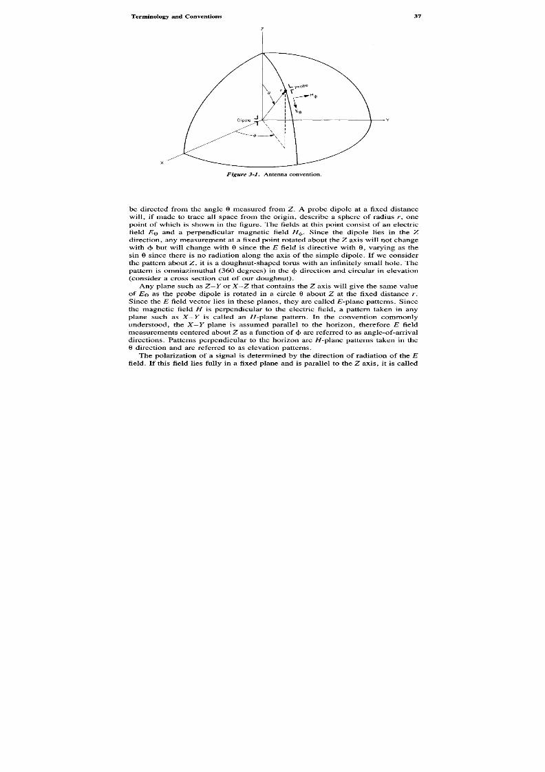
8/8/2019 SciTech - Microwave Passive Direction Finding
http://slidepdf.com/reader/full/scitech-microwave-passive-direction-finding 51/323
be directed from the angle 0 measured from Z. A probe dipole at a fixed distancewill, if made to trace all space from the origin, describe a sphere of radius r, onepoint of which is shown in the figure. The fields at this point consist of an electricfield EQ and a perpendicular magnetic fieldH^. Since the dipole lies in the Z
direction, any measurement at a fixed point rotated about the Z axis will not changewith <\> but will change with 0 since theE field is directive with 6, varying as thesin 6 since there is no radiation along the axis of the simple dipole. If we considerthe pattern about Z , it is a doughnut-shaped torus with an infinitely small hole . Thepattern is omniazim uthal (360 degrees) in the cj> direction and circular in elevation(consider a cross section cut of our doughnut).
Any plane such as Z -Y or X-Z that contains the Z axis will give the same valueof E Q as the probe dipole is rotated in a circle 6 about Z at the fixed distancer.Since the E field vector lies in these planes, they are called £-plane patterns. Sincethe magnetic field H is perpendicular to the electric field, a pattern taken in anyplane such as X-Y is called an //-plane pattern. In the convention commonlyunderstood, the X-Y plane is assumed parallel to the horizon, thereforeE fieldmeasurements centered about Z as a function ofcf> are referred to as angle-of-arrivaldirections. Patterns perpendicular to the horizon are //-plane patterns taken in the9 direction and are referred to as elevation patterns.
The polarization of a signal is determined by the direction of radiation of theEfield. If this field lies fully in a fixed plane and is parallel to the Z axis, it is called
Figure 3~1. Antenna convention.
Dipole

8/8/2019 SciTech - Microwave Passive Direction Finding
http://slidepdf.com/reader/full/scitech-microwave-passive-direction-finding 52/323
vertical. It is referred to as horizontal if it is parallel to either theY or X axis. Asignal is said to be linearly polarized if theE field varies along a line , which happensif we were to move up and down along the length of the dipole, the field being amaximum at the feed point and zero at each dipole tip. If theE field is constantbut varies periodically with time, it is said to be circularly polarized. Right-handcircular polarization sense is defined as the curl of the fingers of the right hand,representing the instantaneousE field as the thumb is pointed in the direction ofpropagation. If theE field vector does not change in amplitude as it rotates in time,it is perfectly circularly po larized. If it reaches a maximum at some angle of rotation ,it is elliptically polarized. The ratio of the maximum to minimum is called the axialratio and is usually expressed in decibels.
When m easuring an antenna field, the polarization of the antenna under test mustbe the same as that of the radiating antenna , this condition being defined as matchedpolarization. Any difference in polarization will cause a cross polarization loss,which may be substantial (theoretically infinite) as in the case of right-handed (RH)circular pattern when compared to left-handed (LH) circular pattern or when avertical pattern is compared to horizontal linear pattern. If an antenna is slantpolarized, its E field vector lies 45 degrees from the Z axis resulting in a 3 dB(half-power) loss when measured by a vertical or horizontal antenna, as will the
measurement of the field of a linearly polarized antenna when measured by acircularly polarized antenna.Circular and slant polarization DF antennas are commonly used for microwave
DF systems since the intercept's polarization is usually know n. There is, of course,the possibility of a complete polarization loss if the sense of the two circularpolarizations are different or the slants of the linear polarization differences are 90degrees opposite as described above. The polarization of the principal lobe of anintercept may differ from that of the side or backlobes, giving the possibility of
further gain or losses in the detection capability of the DF. Gain of an antennarefers to the power contained in the 3 dB or half-power beamwidth and is the valueof the maximum radiation intensity in a given direction referenced to an isotropic(theoretically lossless) antenna that radiates spherically in all directions. Gains areusually expressed in decibels of gain above an isotropic radiator (dBi) assumingmatched polarization. (Gain is sometimes referenced to an ideal dipole althoughthis is not usual.)
When multiantenna systems, such as dispersed spirals or horns, are used to make
angle-of-arrival determinations, it is assumed that the polarizations of all of themeasuring antennas are equal. If this is not the case, the angle determination maybe in serious error. The degree of equality is usually specified by the axial ratiodifferences between antennas in a given set; hence control of axial ratio is important.Since for many antenna types, axial ratio can vary as a function of the angulardistance from the peak of the beam, serious DF errors can result when antennamonopulse comparisons are made off the principal beam axis. These errors becomea function of the angle-of-arrival with respect to the DF systems pointing directionand must be treated in the channel-to-channel unbalance error budget. It is often

8/8/2019 SciTech - Microwave Passive Direction Finding
http://slidepdf.com/reader/full/scitech-microwave-passive-direction-finding 53/323
desirable to be able to measure the polarization of an input signal in this case orwhen high DF accuracies are required.
3.2 SPIRA L ANTENNA
The spiral antenna, which first appears in the literature in the 1956-1961 period(2), is one of the most useful and popular antennas for microwave direction findingsince it exhibits wide RP bandwidth and a relatively constant bandwidth beamwidth,is circularly polarized, and can be easily spatially deployed. It is important tounderstand these general features and the types and modes of the spiral antenna fora full understanding of the usefulness of this type of antenna.
The spiral antenna obtains wide frequency coverage by following the principlesof slow-wave or periodic type structures. Simply stated the concept relates todesigning an antenna that contains, within its design structure, a radiating dipolepair that is essentially frequency self-selecting by the application of an excitingsignal within the frequency capabilities of the antenna. The antenna can perhapsbest be understood by imagining sets of dipole antennas of specific lengths connectedin series, starting with the highest resonant frequency antenna and ending with the
lowest. They are fed by a two-wire transmission line at the high-frequency end, atfeed points A and B as shown (for a planar spiral) in Figure 3-2. Any signal witha 180 degree out-of-phase current applied by the transmission line to the antennawill seek out the dipole pair antenna that resonates, or brings the currents in phase,at the signal frequency passing from the highest frequency antenna paird\-d[ towardthe lowest frequency antenna pairdN-d^ By resonance we mean the point wherethe original out-of-phase current flows in phase as a result of the phase changecaused by propagation over thedifferential distance between the dipole pair and
the feed point. This differential distance assumes that one arm of the pair excites
Figure 3-2. Evolution of series connected dipoles into the archimedian spiral antenna,{a )Dipole pairs.(b) Evolution into spirals with no angles.
a-dipole pairs b-evolution into spiral withno angles
Opentransmission
line

8/8/2019 SciTech - Microwave Passive Direction Finding
http://slidepdf.com/reader/full/scitech-microwave-passive-direction-finding 54/323
an adjacent arm, which when compared to the first arm can be evolved into acircular spiral by bending the finite dipoles, eliminating thed chords, and replacingthem with an arithmetic spiral with an increasing radiusr as shown.
The spiral antenna can be constructed as a pair of metallic radiators or as a pairof slots that are self-complementary, that is, the width of the spirals are equal tothe spacing between them. This concept derives from Babinet's optical principlethat stated that if light were diffracted by a screen resulting in light patterns thatare the complement of the screen pattern, then the sum of the screen and itscomplement would be the pattern without the screen. This is analagous to placinga photographic negative over a contact print aligned so that no pictures can bediscerned. In field theory (3), a radiating conductor is the complement of a conductingsheet that has a slot removed that is exactly equal to the shape of the conductor.If the magnetic field present in the conductor is compared with the electric field inthe slot and if line integrals are performed for each to determine the impedance,the result for a two-arm structure is
z z -nl
ZcZs - —
where
ZQ — input impedance of the radiating conductor
Zs = input impedance of the slot
n0 = 120TT, the impedance of free space
then for the self-complementary case
Zc = Zs = Z spirai
7 - \R °^spiral ~ y —
= no2
Zspiral - 189 oh m s
A spiral antenna can be constructed to cover a frequency bandwidth of over 36to 1 since the above impedance equation is frequency independent, resulting in adesign that has well-behaved voltage standing wave ratio (VSWR) and beam char-acteristics. The geom etry of the construction and the relationship of the spiral dipolesgives rise to a 90 degree phase shift of theE vector with time, yielding a circularpolarization response characteristic. This is a highly desirable attribute for a DFantenna since circular polarization is responsive to the four forms of possible em itter

8/8/2019 SciTech - Microwave Passive Direction Finding
http://slidepdf.com/reader/full/scitech-microwave-passive-direction-finding 55/323
polarization: horizontal, vertical, RH circular, and LH circular. A single spiral willonly respond to the circular polarization response matched to it; however, both RHand LH responses can be received by certain antenna designs. Although dipole andother types of resonant antennas have many of the features of spirals, few offer thewide bandw idth and circular polarization characteristics attainable with this an tenna.The frequency of operation of the spiral is usually defined as the bandwidth overwhich the spiral exhibits circular polarization of the principal beam.
The beamwidth of a typical spiral, when excited in the principal mode, is fairlyconstant at approximately 70 degrees, typically increasing at the lowest frequencyof operation. This is a good number for geographically dispersed antennas, sinceonly four or six antennas are required to cover 360 degrees of azimuth. A specificspiral design, the cavity-backed planar type, can be manufactured by photoetchingcopper-clad dielectric materials using printed circuit techniques, yielding a highdegree of uniformity. This allows good phase match between units and is ideal forinterferometry and phase monopulse applications.
There are basically three commonly used types of spiral antennas: the planararchimedian or arithmetic spiral, the planar equiangular spiral, and the three-di-mensional conical equiangular spiral, shown in Figures 3-3, 3-4, and 3-5, respectively.Each type has several variants: The circular spiral antenna can be constructed in a
square configuration, which for some interferometer systems permits closer spacing ,the planar equiangular spirals can be constructed with differing offset angles fordifferent tracking results, and the conical spiral can be designed with narrow apexangles to permit stacking two as a pair such that the electrical phase center distancebetween antennas can be made less at the high-frequency end of the range, a desirablefeature for interferometer DF systems.
Figure 3-3. Cavity-backed circular planar archimedian spiral antenna. Courtesy of AEL.

8/8/2019 SciTech - Microwave Passive Direction Finding
http://slidepdf.com/reader/full/scitech-microwave-passive-direction-finding 56/323
3.2.1 The Planar Archimedian Spiral
The planar archimedian spiral antenna, shown in Figure 3-3 , consists of a photoetchedcopper Duroid or type GlO dielectric material printed circuit that radiates bidirectionally,perpendicular to the plane of the copper winding. For narrow-band high-gain ap-plications, the antenna circuit board can be backed with a metallic cavity. Forwideband applications, anechoic absorbing material is used in a backing cavity to
Figure 3-4. Circular planar equiangular spiral antenna. Courtesy of Transco.
Figure 3-5. Conical, three-dimensional spiral antenna. Courtesy of AEL.

8/8/2019 SciTech - Microwave Passive Direction Finding
http://slidepdf.com/reader/full/scitech-microwave-passive-direction-finding 57/323
absorb the back wave completely, which is analogous to audio frequencies wherethe back wave of a loudspeaker is absorbed by an insulated cabinet, at the expenseof 3 dB of gain. The figure shows the construction of a commercially availabletwo-arm broadband circular spiral covering the 2-18 GHz range.
The two-arm spiral antenna has been considered (4) to be a balanced two-wiretransmission line that gradually is formed into an antenna by the action of theincreasing radius of an archimedian spiral:
r = roea* (3-1)where
ro = the radius at the start
a = the growth rate
4> = the angle position ofr
Figure 3-6 shows the relationships of circular and rectangular two-arm spiralsand will be used to expand the previous explanations of its operation. The two-wire balanced transmission line does not radiate at the feed point since the currents
are out of phase by 180 degrees causing cancellation. As the transmission lineA-B forms into the two-arm spiral at some pointC, r distance away from the origin0, there will be another pointD, having in common the fact thatC and D both lieon a circle of the same radiusr centered at 0 and on the straight line D O C C . PointC" can also be considered to be at essentially the same radial distance from theorigin as point D if the turns of the spiral are closely (equidistantly) spaced. It isassumed that pointC is excited by C due to its adjacency. The arc distancesADand BC are equal; however, the arc distanceBC is greater. The points essentially
Figure 3-6. Archimedian circular and rectangular spiral relationships.

8/8/2019 SciTech - Microwave Passive Direction Finding
http://slidepdf.com/reader/full/scitech-microwave-passive-direction-finding 58/323
lie on a circle of radiusr measured from the origin 0, therefore, the arc differenceBC from BC is the same as one half of the circumference (C = ir2r) orTTT. Whenthe radius r is equal to X/2ir, the circumference is X, pointC undergoes an additionalphase change of X/2 or 180 degrees with respect to pointB due to the differentiallength (TIT = X/2 when r = X/2TT) and the 180 degree antiphase current conditionoriginating at the feed point is now an in-phase condition atB-C. This causesradiation to take place, which only occurs for in-phase conditions. A similar in-phase condition occurs atD-D'. The radiation occurs inn annular rings or bandsof circumference nX. Since the spiral radius is continuously growing and since thespacing between the conductors equals the width of the conductors, the antenna isa broadband device. Application of a signal at a frequency within the limitationthat its wavelength is less than the maximum diameter will essentially select theappropriate radiating band. Antennas of this type are referred to as slow-wave sincethe signal propagates to where it can radiate.
The spiral antenna is circularly polarized; for every differential group of elementsthat have shifted 180 degrees in phase at the diameter of radiation, there is anothergroup that is in time and space quadrature since the phase of the groups is varyingas a function of the spiral growth rate. This causes a 90 degree phase shift makingthe spiral response circular. The circularity of the response is excellent at bands
within the outer or largest ring degrading to linear polarization near the low-fre-quency or outer band edge and at the high-frequency end if radiation takes placeat the connection of the feed line to the antenna structure.
The number of turns in the spiral is not important as long as the spacing betweenthem is small or equidistant for the complementary case. The lowest frequenciesradiate from the outer or maximum diameter of the spiral; the highest frequencies,near the center. For most applications the outer edges of the spiral should beresistively terminated to ground to prevent a reverse or reflected signal.
In the square spiral shown in Figure 3-6, the same conditions described aboveprevail: Point C is 4/ greater in length from point C, where / is defined as theperpendicular distance from the origin to a side of the square and where it is assumedthe spacing between the turns A/ is constant and much less than /. The circumferenceof the circle drawn at 0 is approximately 8/. As above when / is X/8 the phasechange in current is X/2 or 180 degrees, and radiation takes place (each side of thesquare is X/4). There is a 90 degree phase change for adjacent points, providingcircular polarization. Square spirals can, as discussed above, be placed closer
together than circular spirals; however, phase tracking between square spirals ismore difficult to achieve.
Figure 3-7 shows a rectilinear pattern of a cavity-backed circular spiral antennataken by axially rotating a linearly polarized feed horn while azimuthally rotatingthe spiral under test. The variations or ripple in the patterns represent the axial ratioresponse, which may or may not peak in the vertical or horizontal plane. The axialratio is low (well behaved) at the peak of the beam, degrading somewhat at anglesabout 60 degrees on either side. The back-lobe response is low ( > - 2 0 dB ), whichshows why this type of antenna is popular for direction finding: It is essentially

8/8/2019 SciTech - Microwave Passive Direction Finding
http://slidepdf.com/reader/full/scitech-microwave-passive-direction-finding 59/323
A n g l e
Figure 3-7. Typical pattern of a cavity-back

8/8/2019 SciTech - Microwave Passive Direction Finding
http://slidepdf.com/reader/full/scitech-microwave-passive-direction-finding 60/323
Frequency (GHz)
Figure 3-8. Typical antenna gain versus frequency for a cavity-backed spiral antenna.
unambiguous. It is important also to note that there is practically no squint; thepeak of the beam occurs in the direction of physical boresight.
Figures 3-8 and 3-9 show the gain and beamwidth of the antenna as a functionof frequency over the 2-18 GHz frequency range. The antenna shown here istypical of the type of response obtained in volume m anufacturing, which is sufficientlyreproducible to allow the spiral to be used for dispersed parallel comparison DFsystems.
The operation of the spiral antenna as presented here is often referred to as the"band" theory since it assumes that for every band of circumference ofnk, wheren is a positive odd integer, there will be an in-phase current relationship permittingradiation. The radiation of a spiral fed by a current antiphase transmission line iscalled the odd mode radiation. Whenn is an even number, the currents in the
evoluting transmission line are antiphase, and a null will result. This theory isconceptually acceptable although not completely subject to mathematicalproof.
M
inim
um
lnear
gain
(dBi)
Frequency (GHz)
Figure 3-9. Typical azimuthal beamwidth for a cavity-backed spiral antenna.
3dB Beam
width Degrees)
(Atcenter ofaxialrato)

8/8/2019 SciTech - Microwave Passive Direction Finding
http://slidepdf.com/reader/full/scitech-microwave-passive-direction-finding 61/323
Each mode of radiation exhibits different characteristics. In the first odd mode(n = 1, c = X), the radiation is perpendicular to the plane of the spiral and at a peakalong the principal axis. This mode, which occurs for the diameter, is X/ir (C =X = ITD = X/TT). If the spiral is large in diameter and currents exist past the firstring, additional radiation can take place at the third or fifth and higher modes.
The even modes of radiation of a spiral can be excited by feeding the spiralelements in phase. Assuming the same reasoning as above, radiation will take placeat even diameters, the principal mode beingC = 2X. Since the currents started outin phase, in this mode they will be out of phase atC = X and the radiation patternwill exhibit a null. As the line currents progress, they will be in phase at the evenmode and radiation will occur. This type of spiral antenna is called a normal modedesign and is characterized by a radiation pattern that always exhibits a null alongthe axis and two peaks , displaced in angle as a function of the frequency, as shownin Figure 3-10.
Boresght
Frequency = 6GH3
Vpol
Hpol
Figure 3-10. Typical normal (even) mode pattern of a cavity-backed spiral antenna.

8/8/2019 SciTech - Microwave Passive Direction Finding
http://slidepdf.com/reader/full/scitech-microwave-passive-direction-finding 62/323
3.2.2 The Planar Equiangu lar Spiral
Another solution to the need for wide RF bandwidth antennas is the planar equiangularspiral, first suggested by Rumsey (5) and later characterized by Dyson (6) in 1959.
The concept was prompted by the concept of a frequency independent antenna.Work on the logarithmic periodic antenna by DuHammel and Isbell (7) addedimpetus to the frequency independence theory, as did the development of thearchimedian spiral described above.
The essential idea was to build an antenna using a radiating structure that changeddimensions in a linear proportion to the wavelength. If the shape of the radiatingelement could be defined entirely by angles, the frequency coverage could in theorybe infinite for a lossless structure, since angular variation is unbounded. To define
a practical finite size, however, one length must be specified. Figure 3-11 showsthe development of the idea. If a mathematical spiral is defined as shown, then
ri = roea* (3-2)
Any point r from the origin is proportional to the initial starting point atr0
multiplied by an exponential raised toa$, where a is the growth rate constant and4> is the angular position (as specified in the antenna definitions). Lettingrx defineone edge of a conductor, the second edger2 can be defined by the equation
r2 = roe{a-*> (3-3)
where r2 is the outer edge of the conductor of inner edger as shown in Figure3-12. The conductor has been constructed by letting 8 = 90 degrees. A second
Figure 3-11. Curve for an equiangular spiral.
Figure 3-12. Curve for a spiral conductor.

8/8/2019 SciTech - Microwave Passive Direction Finding
http://slidepdf.com/reader/full/scitech-microwave-passive-direction-finding 63/323
conductor can be added by a similar construction; by letting 8 ^ u / 2 to make thestructure self-complementary, we have
r3 = r ^ - ^ (3-4)
r4 = ^e**-*""8* (3-5)
The lowest frequency of operation is determined by the maximum radiusRresulting in Figure 3-13, showing the complete pattern of an equiangular planarspiral. The radius of the equiangular spiral increases as any conductor goes through360 degrees or
a(4>+2ir)
r = ^ r = e^ (3-6)roe
In general, the Ar is about four with only one and one-half to two turns requiredto wind a broadband (10:1) spiral. The antenna in the figure is self-complementaryand, in fact, was constructed as a slot in copper by Dyson (6) in his early work.
Improved performance of the spiral can be obtained by compound winding; thatis, the feed point starts out as an archimedian spiral, transitions into an equiangularspiral, and finally transitions again into another archimedian spiral, which is ultimatelyresistively terminated at the outer diameter. This is shown for the outer transition
Figure 3-13. Two-arm equiangular spiral antenna.

8/8/2019 SciTech - Microwave Passive Direction Finding
http://slidepdf.com/reader/full/scitech-microwave-passive-direction-finding 64/323
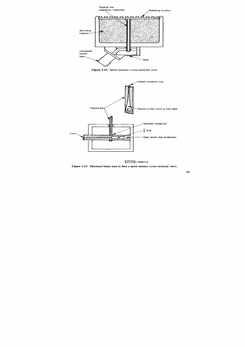
8/8/2019 SciTech - Microwave Passive Direction Finding
http://slidepdf.com/reader/full/scitech-microwave-passive-direction-finding 65/323
Radiating structureTapered ineimpedance tranformer
Absorbingmaterial
Unbalancedcoaxialinput
Nose
Figure 3-14. Spiral antenna—cross-sectional view.
Antenna connection end
Tapered line Tapered printed circuit on both sides
Coax
Indicates connection
^Stub
Open circuit stub termination
Figure 3-15. Marchand balun used to feed a spiral antenna (cross-sectional view).
Dielectric

8/8/2019 SciTech - Microwave Passive Direction Finding
http://slidepdf.com/reader/full/scitech-microwave-passive-direction-finding 66/323
thus an unbalanced conversion is achieved. Good balance is obtained by adjustmentof the dimension of the stub and by minimization of the thickness of the taperedline printed circuit. Wide bandwidth is the result of the very good stub short circuitdue to the ability to obtain a highly reflective termination at the open end. Althoughbalance is obtained, the necessary impedance transformation is not. The 4:1 taperedline transformer performs this function by converting the 52 ohm input line to the189 ohm impedance of the spiral. The antenna radiating structure, which is a circuitprinted on GlO or Duroid dielectric laminate, is carefully soldered to the taperedend lines to maintain a minimum mass at the connection that might radiate byitself.The en tire unit is assembled and backed up by RF anechoic m aterial to fully absorbthe radiated back wave.
The split-taper feed, which offers the advantage of low cost, utilizes a directconnection from the coaxial input line to the tapered line without the balancingtransformer, as shown in Figure 3-16. A coaxial line has been partially etched awayalong length L, effecting both an impedance transformation and a balun action.This type of feed depends upon splitting of the current at the outer conductor anddivision at the septum point as shown. The overall symmetry of the cavity developsa current distribution that achieves a reasonable balanced line effect at the feedpoint. Although simple, spiral feeds of this type usually display considerably greater
pointing error (squint) and axial ratios compared to the true balun-transformerapproach.A normal mode spiral feed is shown in Figure 3-17. Since it is desired to feed
both radiating elements of the spiral in phase, they are connected together and fedby the center conductor of the coaxial line. A launcher, positioned behind the spiralradiating structure, is connected to the outer coaxial conductor to achieve balance.
Radiating structure
Dielectricwith outercoaxremoved
Absorbingmaterial
Outercoax
Septum
Figure 3-16. Tapered line balun feed.

8/8/2019 SciTech - Microwave Passive Direction Finding
http://slidepdf.com/reader/full/scitech-microwave-passive-direction-finding 67/323
Figure 3-17. Normal mode spiral feed.
It is more difficult to obtain low VSWR over broad bandwidths with this type offeed; however, antennas have been built with predictable performance over 9:1frequency rang es. N ormal mode operation can also be achieved by use of a multiarmspiral and an associated feed network, which is generally a more popular methodsince normal mode operation of a spiral is usually associated with comparison withother derived spiral beam s, all of which are obtainable in multimode configurations.
3.2.4 Conical Equiangu lar Logarithmic Spirals
The conical logarithmic equiangular spiral antenna results directly from the projectionof a planar equiangular spiral on a cone. From Figure 3-18, this projection may beexpressed as
i _ e(a sin 6O)(}> ( 3 - 7 )
where
11 = one edge
6 = one-half the apex angle
a = the wrap rate8 = the spiral width (usuallyTT/2 for the self-complementary case)
Launcherconnected tocoaxial outerconnector
Both feed points connectedto center coax conductor
Radiatingstructure
Absorber

8/8/2019 SciTech - Microwave Passive Direction Finding
http://slidepdf.com/reader/full/scitech-microwave-passive-direction-finding 68/323
The second edge, I2, may be defined as
I2 = e(a sin e«) (<!>-&) (3-8)
The second arm of the spiral is developed by rotation and construction 180 degreesaway. All edges of the spiral hold a constant angle a with a radial line, that is, the
radiator elements are tightly wrapped around the cone.As in the case of the planar spiral, the antenna must be fed in current antiphaseto excite the odd mode of radiation. Even mode radiation can be excited by parallelin-phase current feed, resulting in a null along the axis. The impedance of aself-complementary spiral is approximately 165 ohms (10). Radiation from the antennain the commonly used odd mode is off the axis in the pointing direction of the cone(—Z direction) and is circularly polarized degrading to elliptical polarizer at thebeam width ex tremes. T he lowest frequency of operation is determined by the base
diameter B when it equals three-eighths wavelength. The highest frequency ofoperation occurs when the truncated cone diameterb is one-fourth wavelength.Typical manufactured conical spirals (11) exhibit 0-2 dB gains and cover up to an11:1 bandwidth using apex angles of about 30 degrees. H igher gains can be obtainedby mounting the conical spiral on or below a recessed ground plane, the lattertechnique often being used for flush-mounted applications. When the apex angle(equals twice 0O) becomes TT/2, the conical spiral evolves into the planar spiral,which is the limiting case. Unlike its counterpart, however, the conical spiral tends
to radiate unidirectionally against a ground plane, eliminating the need for anechoicabsorbing materials.
Figure 3-18. Conical equiangular spiral antenna.

8/8/2019 SciTech - Microwave Passive Direction Finding
http://slidepdf.com/reader/full/scitech-microwave-passive-direction-finding 69/323
Since the process of radiation follows the previously described "band" theory,the conical spiral radiates at what is known as the "active region" with a center ofphase that positions itself linearly along the antenna axis as a function of frequency,permitting two conical spirals to be pointed toward each other in an array, as shownin Figure 3-19. This array is very useful for interferometer applications since awider unambiguous bandwidth can be obtained as a result of the closer spacing(d < X/2) at the high-frequency band edge. By interconnection with a 180 degreehybrid, sum and difference monopulse outputs can be obtained over an extremelylarge bandwidth. An extensive study of this approach by Hahn and Honda (12)reached the conclusion that practical DF systems could be made, although withonly a fair degree of accuracy, due in part to the phase tracking of componentryavailable at that time. The more popular configuration for conical spirals is inamplitude comparison monopulse systems where the greater gain of the conicalspiral is important.
3.2.5 Multimode and Multiarm Operation of Spirals
A single spiral can be made to appear as an array of many to provide multipleoutputs for different types of monopulse DF systems. This can be done by exciting
Figure 3-19. Center of phase of two pointed conical spiralsd, moves with frequency d = f(wt).

8/8/2019 SciTech - Microwave Passive Direction Finding
http://slidepdf.com/reader/full/scitech-microwave-passive-direction-finding 70/323
multiple modes of operation in a simple two-wire spiral or by the use of multiarmspirals. Both cases require the use of combinations of couplers and hybrids, which,because of their narrow bandwidths, limit the overall bandwidth obtainable. Thistype of use is important, however, since it is possible to develop highly accuratetargeting and guidance systems in a small space utilizing a minimum of antenna"real estate," often a key consideration in missile and spacecraft applications.
First attempts to excite dual modes in a simple two-arm spiral were describedby Kaiser et al. (13) in a passive type direction finder. The concept was to exciteboth the even and odd modes simultaneously in a two-arm spiral by means of ahybrid, recognizing that there would be two distinct patterns generated. The first,due to odd mode excitation, would be the familiar beam pointed along the axis
perpendicular to the plane of the antenna. The second would be the even or normalmode pattern, a doughnut-shaped torus with a null along the axis . Figure 3-20 showsthe phase relationship between the two patterns as a function of revolutionaround the Z axis or circumference of the spira l. The odd or first mode angle 4>travels 360 degrees, while the even or second mode angle traverses 2cf> or 720degrees. The measurement of thedifference in phase between the two modestherefore will give the angle 4>. The amplitude difference between the beam andthe torus provides 6. Knowledge of these two angles provides an unambiguous
measure of the angle of arrival of a signal.Although conceptually attractive from many points of view, this system sufferedlimitations due to phase variations at the extremes of the beams and bandwidth
Figure 3-20. Phase relationships of a single-arm dual mode excited spiral antenna.
First modeSecond mode

8/8/2019 SciTech - Microwave Passive Direction Finding
http://slidepdf.com/reader/full/scitech-microwave-passive-direction-finding 71/323
limitations due to the lack of wideband hybrids at that time. On the positive side,there is the potential for better ellipticity tracking since both modes use the sameantenna. The possibility for good accuracies along the null axis makes this antennauseful for narrower bandwidth guidance systems. A second approach to simultaneousmultibeam DF makes use of a multimode, multiarm spiral in conjunction with acorporate feed network to utilize more accurate processing techniques.
Multiple-arm spirals can be configured for any of the types of planar or conicalantennas discussed. The concept is simple enough: Four or more spiral arms arewound from the center following the equations for antenna growth presented above.Each arm of the spiral is separately fed by a port of an excitation matrix designedto produce simultaneous excitation of both odd and even modes by the action ofthe sum and difference properties of a 180 degree hybrid. Practical considerations,however, have led to the common use of four- and six-arm spirals. Reasons forthis are obvious: It is difficult to feed m ore arms at the center; conical spirals becom elimited in high-frequency response due to the added truncation of the cone toaccommodate more feeds; planar spirals become less self-complementary and exhibitdifferent impedances, and so on.
Much work has been done to try to build multiple-arm antennas. The literatureabounds with attempts to feed the spirals from the outside diameter (1 4-1 6); how ever,
unwanted bands of radiation develop, restricting the RF bandwidth and causinghigh VSWR variations since the outside feed impedances vary with frequency. Forthese reasons we shall confine our discussions to the two most popular multiarmspirals, the four-arm sum (S) and differences (A) feed and the six-arm amplitudecomparison type. Both designs are true monopulse approaches to passive directionfinding and find practical use in many applications.
When a four-arm spiral is excited by a dual-mode excitation network, a sum orprincipal mode will develop, peaking along the bore-sight axis in a manner similar
to the two-arm spiral described above. (This is not to be confused with the balun-fed spiral, which , although developing the same pattern, does so directly as opposedto summing process used in this case.) The network that accomplishes this is shownin Figure 3-21. Three hybrids and a 90 degree phase shifter form the excitationnetwork. A portion of all elements is progressively summed and identified as thesum (2) output. The first level of hybrids form the 180 degree phase difference ofopposing arms 1-3 and 2 - 4 , one of which is shifted 90 degrees and added to theother to form the difference pattern.
The angle off boresight is 9; the angle around the circumference of the antennais <|>. If a signal is rotated around 4> about the principal beam around bore sight,the antenna will register a 360 degree variation as indicated in Figure 3-22, whichis a view of the phase variation in theX- Yplane parallel to the flat plane of theantenna. [Note that this is precisely the same pattern as that of the two arm dueexcited spiral discussed previously (Fig. 3-20).] This variation is called the firstmode that undergoes a 360 degree phase change for a 360 degree spatial changeand corresponds to the sum pattern defined as
/(4>) = e> * (3-9)

8/8/2019 SciTech - Microwave Passive Direction Finding
http://slidepdf.com/reader/full/scitech-microwave-passive-direction-finding 72/323
Figure 3-21. Four-arm spiral spatial monopulse direction finder.
The difference (A) or second mode pattern, however, undergoes a variation of 720degrees for the same 360 degree spatial variation for the second mode circle,corresponding to
G = G($)e j2 ^ (3-10)
The relative phase difference between the two modes for the four-arm case is 360degrees, and measurement of this difference phase will yield cf>. This is the same
Monopulse output
Excitationmatrix
Four armplanar spiral
Figure 3-22. Phase relationships of the four-arm spiral.
First mode
Second mode
8/8/2019 SciTech - Microwave Passive Direction Finding
http://slidepdf.com/reader/full/scitech-microwave-passive-direction-finding 73/323
as for the two-arm case previously discussed; Figures 3-20 and 3-22 are actuallyidentical. The four-arm network is more predictable, however, and is the preferredtechnique.
The ratio of the sum and difference amplitudes will yield the angle 6; however,since it is the angle off bore sight between the two patterns in any direction, it willbe ambiguous unless§ is used to supply a correction to derive the actual elevationangle. A processor designed to accomplish this is described in Chapter 4, Section4.4.
One of the limitations of the two-arm spiral in multimode applications is theincrease in axial ratio that occurs at far angles on either side of the boresight. Theproblem is exacerbated by the narrow (70) beamwidth of the peak pattern since theaxial problem becom es worse as a percentage of beam width. One successful solution(17) has been to use a six-arm spiral to array the patterns, achieving agreater effective beamwidth per antenna of about 90 degrees. Figures 3-23 and3-24 show the six-arm excitation matrix and the total processing function resultingin the development of four amplitude beams spaced 90 degrees from each otherand corresponding to a four-quadrant DF system. Although this system appearscomplicated, it can be implemented using printed circuit technology resulting in ahighly compact and production-repeatable design. Figure 3-25 shows the patterns
resulting from this configuration, which are essentially 90 degree cardioids withacceptable axial ratios along the boresight. Deterioration of the axial ratio offboresight, however, still limits this approach to hemispherical measurements suchas radar tail warning or missile guidance.
The processing for the above system can make use of a summed (S) output,which will be the approximate equivalent of the output of a simple spiral, asdiscussed. It is interesting to note that there will always be one less useful beamthan there are arms in multiarm spiral configurations. This is due to the fact that
n — 1 excitations are required for the noninfinite number of elements case. In theabove six-arm spiral, only five useful patterns are available, for example.
3.2.6 Millimeter Wave Spirals—The Antector
Attempts to extend the high-frequency coverage of the spiral antenna into themillimeter frequency range have, up to the present, met with limited success.Although it is possible to get planar archimedian spirals to exhibit the familiarGaussian patterns past 100 GHz, feed networks and especially the Marchand balunhave not been successfully developed. Transverse electric and magnetic (TEM)mode coaxial cable exhibits high losses and develops extraneous modes of operationabove 40 GHz, making this type of transmission line useless at higher frequencies.Waveguide feeds are limited in coverage at the low end of a frequency range bythe guide cutoff frequency and at the high end by unusable modes. Attempts toincrease the frequency of coverage of waveguides by ridging techniques are generallytoo lossy.
A more fundamental approach has been developed by the design of a combinedantenna and detector (18), which has been named the antector, a euphemism that

8/8/2019 SciTech - Microwave Passive Direction Finding
http://slidepdf.com/reader/full/scitech-microwave-passive-direction-finding 74/323
Figure 3-23. Excitation matrix for six-arm spiral antenna.
describes its operation. Basically, the idea consists of mounting a beam lead diodedetector directly at the inner center feed point of a wideband MM wave spiral andcoupling off the resulting detected video from one outer arm. This eliminates allof the problems of coaxial feed and all of the difficulties attendant to the use ofmany different suboctave band coverage waveguides. The other arm is used as aconvenient point for application of direct current (DC) bias for the diode. Botharms are terminated to prevent RF reflections and decoupled to pass the bandwidth
Beam formingnetwork
Four spacequadrature beams(«9O°cardioids)
Beamcompensaton
network
Antennaprocessngnetwork
6 Arm
spiralantenna

8/8/2019 SciTech - Microwave Passive Direction Finding
http://slidepdf.com/reader/full/scitech-microwave-passive-direction-finding 75/323
F i g u r e 3 - 2 4 .A n t e n n a p r o c e s s i n g n e t w o r k f o ra s i x - a r m s p i r a l y i e l d i n gS + A a n d X - A o u t p u
of the millimeter wave detected video, which occupies a wide bandwidth associatedwith the narrower pulses found in this range. The concept is illustrated in Figure3-26, which is a diagrammatic representation of the approach. The detector diodeis chosen to present an impedance of approximately 100 ohms, and, since currentcan flow through it, acts like a balanced feed. The principal or odd mode of thespiral is excited causing the antenna to develop a beam that is peaked along the
boresight of the axis perpendicular to the plane of the printed spiral elements. Asfor all wideband spirals, it is necessary to mount the radiating printed circuit infront of an anechoic absorbing material to cancel the backwave.
Output
Output
Antenna
Boresightaxis
Right- eft plane
Up-down planeTarget
Figure 3-25. Forward-looking application of four-beam six-spiral antenna and feed network.
= 90°Phase Shifter
=50 OHM Termination= Antenna

8/8/2019 SciTech - Microwave Passive Direction Finding
http://slidepdf.com/reader/full/scitech-microwave-passive-direction-finding 76/323
Figure 3-26. Diagrammatic representation of the antector showing electrical connections.
Figure 3-27 is a photograph of a beam lead diode mounted on a spiral that coversthe frequency range from 18 to 100 GHz. Patterns have been taken at 20, 40, 65,and 100 GHz for the model photographed and are shown in Figures 3-28 to 3-31.A beamwidth of approximately 60 degrees is obtainable over this band with all ofthe characteristic properties of a spiral, low sidelobes, and a good axial ratio.Sensitivities in the order of lower band antennas and separate detectors can be
achieved; however, the antector's sensitivity must be corrected for the diode'sefficiency loss at MM wave frequencies.There are two potential problems with the antector: possible burnout from high-
power illuminators and an undesirably slow sensitivity rolloff at the low-frequencyband-end limit. Since the antector is not shuttered or shielded, strong out-of-bandsignals readily illuminate the detector. Fortunately, this causes a decrease in thediode's impedance, which tends to reflect some of the power at the diode, thusprotecting it. Data show that protection up to a level of +25 dBm is achievable.
(This problem is solved in standard detectors by the incorporation of a limiter diodein shunt with the detector, a technique not feasible here.) The low-frequency rolloffcan be improved by careful design.
The advantage of the antector is the wide and fairly predictable performanceattainable in a low-cost millimeter sensor. When used in warning receiver applications,it can indicate the presence of high-frequency threats that could not be as readilydetected over such wide bandwidths. The detection probability of this methodcompares favorably to or is better than narrow-band scanning superheterodynetechniques for strong signals.
Videoand R F. termination
Dode mounted in center
Videoout
Bias
R F. termination

8/8/2019 SciTech - Microwave Passive Direction Finding
http://slidepdf.com/reader/full/scitech-microwave-passive-direction-finding 77/323
Figure 3-27. Antector: A combined cavity-backed spiral antenna and detector. Courtesy of AEL.

8/8/2019 SciTech - Microwave Passive Direction Finding
http://slidepdf.com/reader/full/scitech-microwave-passive-direction-finding 78/323
A n g l eF r e q u e n c y
: 2 6 G H
Figure 3-28. Azimuth pattern coverage of th

8/8/2019 SciTech - Microwave Passive Direction Finding
http://slidepdf.com/reader/full/scitech-microwave-passive-direction-finding 79/323
A n g l eF r e q u e n c y :4 0 G H
Figure 3-29. Azimuth pattern coverage of

8/8/2019 SciTech - Microwave Passive Direction Finding
http://slidepdf.com/reader/full/scitech-microwave-passive-direction-finding 80/323
A n g l eFrequency6 5 G
Figure 3-30. Azimuth pattern coverage of the antec

8/8/2019 SciTech - Microwave Passive Direction Finding
http://slidepdf.com/reader/full/scitech-microwave-passive-direction-finding 81/323
A n g l eF r e q u e n c y !
Figure 3-31. Azimuth pattern coverage o
Next Page

8/8/2019 SciTech - Microwave Passive Direction Finding
http://slidepdf.com/reader/full/scitech-microwave-passive-direction-finding 82/323
3 .3 HORNANTENNAS
A horn antenna is basically a transition from a transmission line to free space,taking into account the requisite impedance and field requirements. A brief descriptionof transm ission line theory will illustrate how this transition can take place for bo thcoaxial and waveguide elements.
3.3.1 RF Transmission Lines
The following is an expository explanation of transmission lines in general andwaveguides in particular. The explanations have been designed to be pertinent tothe discussions on horns, biconical radiators, and polarizers and can be augmentedby reference to many available texts (see Ref. 19).
Coaxial cable is perhaps the most useful type of RF transmission line since itexhibits a principal mode of propagation , called the transverse electric and m agnetic,or TEM mode, capable of operating from DC to the high microwave frequencies.Figure 3-32 shows the construction of familiar coaxial cable, which consists of an
Outer plasticprotective jacketuter conducter(shield or solid)ielectric spacingInner conductor
a) Construction
E FieldH Field
TEM
b) The principal mode of operation
Figure 3-32. Coaxial transmission line,(a) Construction, (b) Principal mode of operation.
Previous Page
8/8/2019 SciTech - Microwave Passive Direction Finding
http://slidepdf.com/reader/full/scitech-microwave-passive-direction-finding 83/323
inner conductor centered within an outer conductor, that may be braided for flexi-bility. A solid copper conductor is used for semirigid lines. The area between thetwo conductors is filled with a low-loss dielectric material, usually polyethylene orTeflon, which may be solid or made of beads. Flexible line has an additional outerpoly vinyl chloride plastic protective coating , whereas sem irigid line may be p lated.
Energy propagates in the dielectric as the frequency increases. TheE and Hfields are traverse to the direction of energy propagation; that is, theE and H fieldslie in a plane perpendicular to the signal flow. The two conductor sizes and thecharacteristics and separation of the dielectric material determine a "characteristicimpedance," which is a physical property of and is used to identify the line. Whenterminated in its characteristic impedance, the line exhibits a resistive input impedanceat the source end for a resistive termination at the far end.
Coaxial cable is limited, as the frequency increases, due to a gradual buildupof loss in the dielectric material needed to support the inner conductor. There isalso additional ohmic loss in the two m etallic conductors due to surface "skin effect"as the signal travels down the line. At very high frequencies, near 30 to 40 GHz,coaxial cable exhibits additional cylindrical waveguide modes, which impose anupper frequency boundary. Very small dimensioned cable is available to overcomethis problem; however, the loss is high (typically greater than 0.5 dB/ft), makinglong cable connections impractical.
Waveguide is the common form of microwave transmission line used becauseit has low loss and is dimensionally suitable at microwave frequencies. The low-loss properties derive from the use of air or gas as the dielectric in a conductinghollow tube or guide. Propagation of RF energy occurs as described by wave theory.Poynting's theorem can be used to give the direction of the power flow or flux atany point in a dielectric medium, as a function of the direction of the electric andmagnetic fields. IfE and H are the values of the fields associated with an alternating
current at any point, then the powerP in the dielectric is
P = EH sin 6 (3-11)
where
6 = the angle betweenE and H
or in vector notation,P = (E x H) (3-12)
which is the cross product of the E and H vectors.This formula follows the right-hand rule; that is, if the fingers of the right hand
curl in the direction of E to H, the thumb points to the direction of power flow.From this it is clear that propagation or movement of power takes place. (This isalso true for the coaxial cable.) If a conductor is placed near the propagating wave,any component of the electric field parallel to the conductor sees an equipotentialconducting surface that acts as a short circuit reducing theE field rapidly to zero.

8/8/2019 SciTech - Microwave Passive Direction Finding
http://slidepdf.com/reader/full/scitech-microwave-passive-direction-finding 84/323
If any component of theH field flows perpendicular to the conductor it encountersa short circuit that causes it to fall rapidly to zero. In a hollow rectangular w aveguide,which is bounded by conductors on all four sides, bothE and H fields cannot betransverse with respect to the direction of propagation due to the above effects;therefore TEM waves do not exist in waveguides.
Two classes of waves do propagate in a waveguide, however—the transverseelectric TEmrt and transverse magnetic TMm n. (The British call these wavesH andE.) Subscript m refers to the num ber of half-wave variations in theX direction, andsubscript n refers to the number of field variations in theY direction. (To preventconfusion and to follow current convention, theX direction will be consideredparallel to b, and Y will be parallel toa as shown in Figure 3-33.) The TEmn wavecontains the electric field vector perpendicular to the direction of travel (transverse)with no net component of theH field in the direction of propagation. The TMmn
wave has the magnetic perpendicular (transverse) with no net component of theelectric field in the direction of propagation. A waveguide therefore bounds or
Electric flux Magnetc flux
Fluxout of pageFluxinto pagea) Longitudinal top view
Electric flux
Magnetic flux
Electric fluxMagnetc flux
b)End view of guide
Figure 3-33. Representation of the TEi0 (principal) mode of propagation in a rectangular waveguide.(a ) Longitudinal top view; (b) end view of guide

8/8/2019 SciTech - Microwave Passive Direction Finding
http://slidepdf.com/reader/full/scitech-microwave-passive-direction-finding 85/323
contains the RF energy allowing only certain modes to exist due to the short-circuiteffects of the conducting walls of the guide.
Of all the modes possible, one mode—the TEi0, or principal, mode shown inFigure 3-33—propagates at the lowest frequency. From Figure 10-33a, it may beseen that moving along the length of the guide, the electric field reverses its directionwhile the magnetic flux forms circular flows in alternating directions. The electricfield crosses over (is zero) at the center of each magnetic flux circle. Note that themagnetic flux is bent when it is perpendicular to a wall due to absorption of theperpendicular wave, allowing only the magnetic flux parallel to the wall to flow.
From Figure 10-33Z?, we determine that the electric field is a maximum at thecenter of the guide (more lines) and diminishing to zero at the conducting boundaries.The value for m = 1 indicates that there is one-half wave ofE in a cross-sectiontransverse to the power flow along the widthb. The n = 0 indicates that there isno variation of E along the a dimension.
The cutoff frequency is defined as the frequency of the TEi0 mode or as thefrequency of maximum or near-infinite attenuation. The lowest or principal modeoccurs when
Xc = 2b Vixe =* 2b for air (3-13)
where
|x = the guide dielectric permeability
€ = the dielectric constant
This makes the waveguide essentially a high-pass filter, propagating all frequencieshigher than Xc where practical attenuation occurs. The useful operating range formost TEmrt guides is from 1.3 times the cutoff frequency to 0.9 times the cutofffrequency of the next higher mode. This results in about a 1.5:1 ratio for narrowheight (height ~ bl2) guides. High-frequency propagation is limited by the appear-ance of higher-order TE and TM modes that limit simple waveguide to suboctavecoverage. These properties are often made use of in the design of waveguide filtersand couplers.
The height a determines the power-handling capacity of the waveguide since itmust withstand the maximumE field strength. The ohmic loss of the guide occursas the wave propagates along the length of the guide. The current of theH fieldperpendicular to the direction of wave propagation penetrates the wall, while theE field drops to zero at the conducting boundaries as described. The depth ofpenetration of the RF energy is
8 = in meters (3-14)V IT |x/cr

8/8/2019 SciTech - Microwave Passive Direction Finding
http://slidepdf.com/reader/full/scitech-microwave-passive-direction-finding 86/323
Table 3-1. Wavelength Characteristics of Rectangular and Circular Waveguides
Rectangular Guide0 Circular Guide**
\c(cuto ff wavelength) (attenuation is infinite) 2.0b 3.41 rXg(usable guide wavelength) 1.6b 3 . 2 0 r\n(shorte st wavelength before next mode) 1.1b 2.8 ra b is guide width.b r is radius of circular guide.
whe re
(Ji = 4TT X 1 0~7 for copper
a = 5.8 X 10⁷ for copper
f = frequency in MH z = 3000 X 10'
For exam ple, at X = 10 cm , 8 = 1.2 x 10~4 cm, which shows that the penetratingfields and currents are at "skin" depth. Losses in a guide or coax operating at high
frequency occur at the surface of the conductors making silver, rhodium plating orgold flashing popu lar techniques to reduce loss due to the high conductivity of thosemetals. Table 3-1 gives the relationships for the principal propagating modes ofrectangular and circular guides for references.
The operating frequency of a waveguide can be made lower by adding one ortwo ridges as shown in Figure 3-34. The addition of the ridges reduces the power-handling capability of the waveguide, but for receiver and lower power transmitterapplications it can be useful. The ridges can be continued into the horn for w ideband
applications. Losses in the guide using this approach are greater, as described inRef. 20.
a) Single ridge
b)Doube ridge Figure 3-34. Ridge-loaded waveguide, (a ) Single ridge; (b) double ridged.

8/8/2019 SciTech - Microwave Passive Direction Finding
http://slidepdf.com/reader/full/scitech-microwave-passive-direction-finding 87/323
3.3.2 Single-Mode Horn Antennas
Horn antennas find use in passive DF systems chiefly because of the gain improve-ment and pattern directivity they offer. In transmit applications, power-handling
capability of the horn is important; how ever, in receiving applications, w e are usuallyconcerned with pattern ratios to form beams and predictable beamwidths both fordirect signal measurement and for the purpose of illuminating passive reflectorsthat can shape and move the horn's beam as desired. A horn antenna is a transitionstructure that conducts a signal in a waveguide transmission line to an unboundedmedium, such as air, where the signal is free to radiate. A waveguide has a characteristicimpedance that must be matched to that of free space (1207T ohms). Since, byRayleigh's reciprocity theorem, an antenna is reciprocal (it works the same way
when transmitting as when receiving); it will receive an inbound wave from freespace and will transition it into a waveguide as well as carry an outbound wavefrom a transmitter to an antenna where it is radiated. The pattern and gain will bethe same for either case.
In passive DF receivers, it is generally desirable to obtain maximum frequencybandwidth and control of the antenna's pattern gain and symmetry. Horn antennas,therefore, find application mainly in arrays where they are used to generate eithera linear (in-line) or circular phase front with the mechanical advantage of closeproximity "stacking." This is shown in Figure 3-35 for a lens-fed array where aset of closely spaced waveguides radiate, each acting directly as an antenna to
Figure 3-35. Waveguide array. Courtesy of Raytheon Corp.

8/8/2019 SciTech - Microwave Passive Direction Finding
http://slidepdf.com/reader/full/scitech-microwave-passive-direction-finding 88/323
generate a linear wave front. In rotating passive reflector systems, hornsare usedwith rotary joints to illuminate a flat or focused reflector in a prescribed way toobtain specific patterns.
Gain is provided by the aperture size of a horn if the aperture fieldsare uniformin phase and amplitude. In this case, the beamwidth (BW) <\> az in either the x or ydirection 9 ei, as shown in Figure 3-36 is simply
V 3 XB W , = - - (3-15)
V 3 XB W 0 = ^ r T (3-16)
2 dy
The highest gain of the antenna is
G = ~A (3-17)
whereG = the uniform aperture gain
A = the physical area (dxdy) of the aperture
Feed point
Reference plane
Z
Directionof
propagation
Horn
Aperture= dxdx
Figure 3-36. Reference diagram for a horn antenna.

8/8/2019 SciTech - Microwave Passive Direction Finding
http://slidepdf.com/reader/full/scitech-microwave-passive-direction-finding 89/323
Realizable gain, however, will be considerably lower due to ohmic and reflectionlosses. Practical numbers allow for 50% efficiencies. A useful relationship for gainas a function of the beamwidth for most EW applications where direct feed is usedis
O - *g>
where
<\> = azimuthal beamwidth (degrees)
9 = elevation beamwidth (degrees)
A relationship may be found for reflector feeds in Ref. 10, where gains using 2 6,00 0for the numerator in Equation (3-18) are good approximations for the illuminatingefficiency used.
The minimum sidelobe levels of a constant illumination pattern is of the sixx/x form which places the first sidelobe at -13.3 dB below the main beam. This isnot much dynamic range for direction finding; therefore, to provide lower side-lobes, nonuniform illumination of the aperture obtained by varying the E field ina cos or cos2 manner is often used. Table 3-2 lists typical sidelobes levels fordifferent illuminations.
Variation of the illumination can be seen to make substantial differences in theback- and sidelobe levels. These factors are vital in radar systems where reflectorillumination is important; however, for passive DF systems using multiple directradiating antennas, it is often possible to use the simple type of uniformly illuminatedopen-ended waveguide.
There are three basic types of rectangular waveguide fed sectorial horns: theEplane, the H plane, and the pyramidal as shown in Figure 3-37. TheE plane givesa narrow elevation and wide or fan azimuth beam for application in height-finderradar systems and for sidelobe inhibition. TheH plane horn gives a narrow azimuthand wide fan beam elevation pattern and is most popular for passive DF applicationswhen only azimuthal angle of arrival is required, since maximum intercept probability
Table 3-2. Illumination vs. Side Lobe LevelType of Illumination Illustration Side-Lobe Level (dB)
- 1 3 . 3
- 1 9 . 5
- 2 3 . 1
- 3 1 . 7
Uniform
11.4 dB taper(r = .862)
Cos
Cos2

8/8/2019 SciTech - Microwave Passive Direction Finding
http://slidepdf.com/reader/full/scitech-microwave-passive-direction-finding 90/323
Figure 3-37. Types of rectangular horn antennas:(a ) £-plane sectorial horn, (b) //-plane sectorial horn.(c) Pyramidal sectorial horn.
will be obtained in the vertical plane due to the wide elevation coverage. Thepyramidal horn can prov ide a sym metrical beam (<j> = 9) . This is desirable for high
gain narrow pencil beam raster scan systems where field of view is traded for gain,especially at millimeter wave frequencies where RF preamplification and low noisefigures are difficult to obtain.
The polarization of a horn is determined by the direction of theE field vector,which is initially established by the waveguide feed. The polarization can be shiftedto slant linear (E field at 45 degrees) by means of an internal or external polarizer,which converts the direction of the arrivingE field to that of the antenna at theexpense of some gain. Waveguides can also be twisted 45 degrees and fed to a
pyramidal horn for slant linear polarization, which is a compromise. Various othermethods to make horns respond to many linear and circular polarizations are used,
c)Pyramda sectorial horn
E-Field
E-Field
b) H-Pane sectorial horn
E-Fed
a) E-Pane sectorial horn
Wavegude
Wavegude
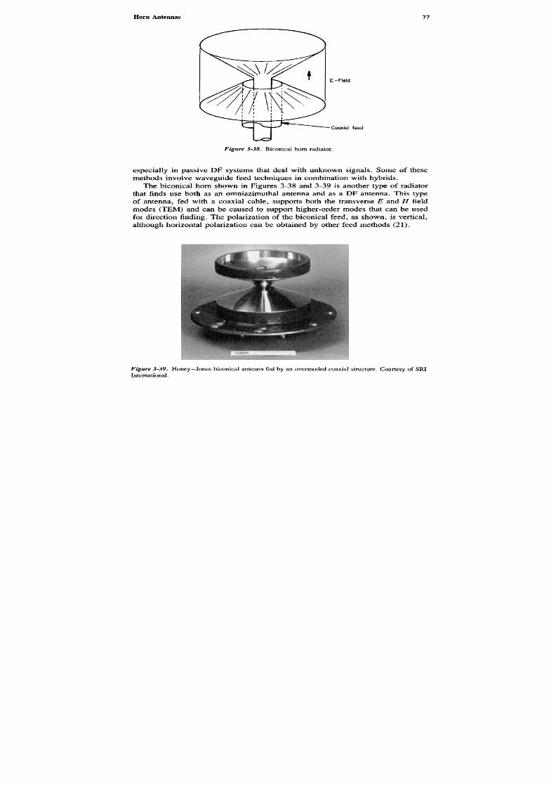
8/8/2019 SciTech - Microwave Passive Direction Finding
http://slidepdf.com/reader/full/scitech-microwave-passive-direction-finding 91/323
Figure 3-38. Biconical horn radiator.
especially in passive DF systems that deal with unknown signals. Some of thesemethods involve waveguide feed techniques in combination with hybrids.
The biconical horn shown in Figures 3-38 and 3-39 is another type of radiatorthat finds use both as an omniazimuthal antenna and as a DF antenna. This typeof antenna, fed with a coaxial cable, supports both the transverseE and H fieldmodes (TEM) and can be caused to support higher-order modes that can be usedfor direction finding. The polarization of the biconical feed, as shown, is vertical,although horizontal polarization can be obtained by other feed methods (21).
E-ReId
Coaxial feed
Figure 3-39. Honey-Jones biconical antenna fed by an overmoded coaxial structure. Courtesy of SRIInternational.
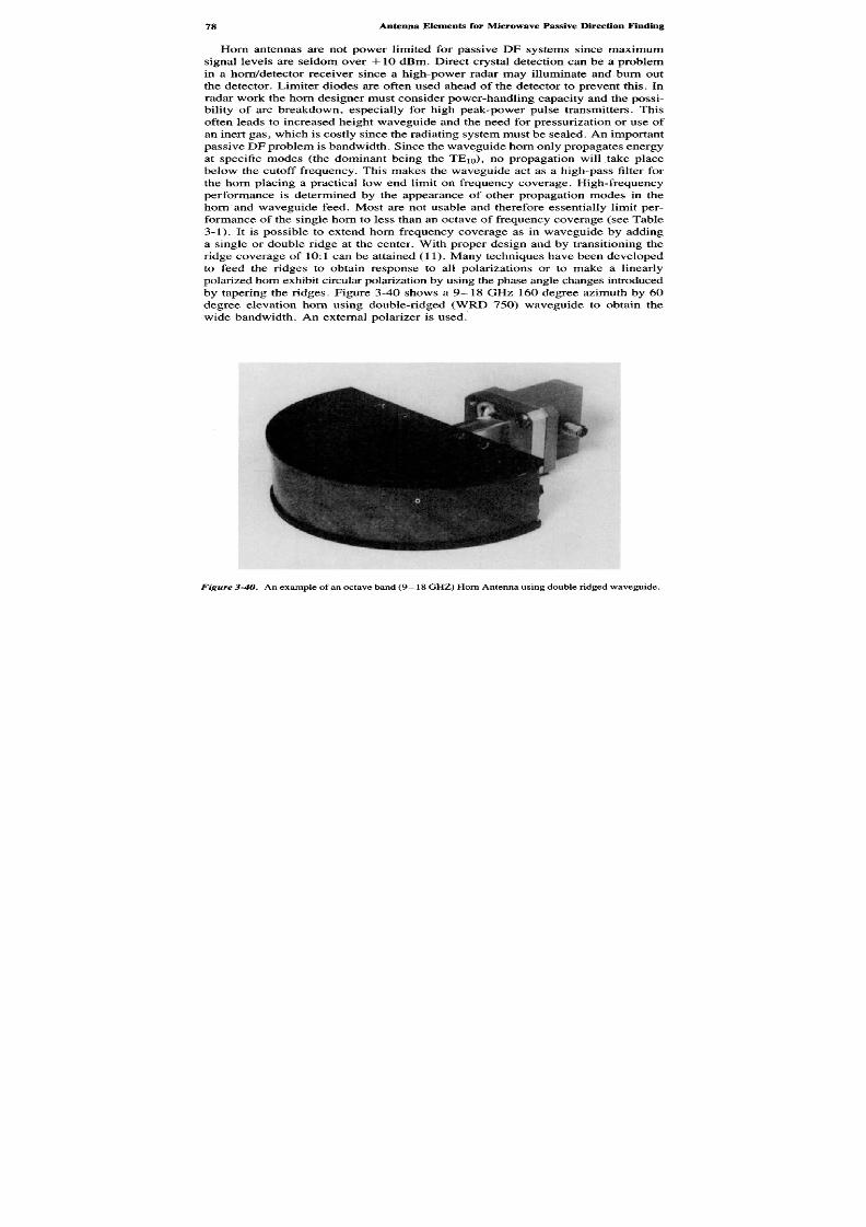
8/8/2019 SciTech - Microwave Passive Direction Finding
http://slidepdf.com/reader/full/scitech-microwave-passive-direction-finding 92/323
Horn antennas are not power limited for passive DF systems since maximumsignal levels are seldom over +10 dBm. Direct crystal detection can be a problemin a horn/detector receiver since a high-power radar may illuminate and burn outthe detector. Limiter diodes are often used ahead of the detector to prevent this. Inradar work the horn designer must consider power-handling capacity and the possi-bility of arc breakdown, especially for high peak-power pulse transmitters. Thisoften leads to increased height waveguide and the need for pressurization or use ofan inert gas , which is costly since the radiating system m ust be sealed. A n importantpassive D F problem is bandwidth. Since the waveguide horn only propagates energyat specific modes (the dominant being the TE10), no propagation will take placebelow the cutoff frequency. This makes the waveguide act as a high-pass filter forthe horn placing a practical low end limit on frequency coverage. High-frequencyperformance is determined by the appearance of other propagation modes in thehorn and waveguide feed. Most are not usable and therefore essentially limit per-formance of the single horn to less than an octave of frequency coverage (see Table3-1). It is possible to extend horn frequency coverage as in waveguide by addinga single or double ridge at the center. With proper design and by transitioning theridge coverage of 10:1 can be attained (11). Many techniques have been developedto feed the ridges to obtain response to all polarizations or to make a linearly
polarized horn exhibit circular polarization by using the phase angle changes introducedby tapering the ridges. Figure 3-40 shows a 9-18 GHz 160 degree azimuth by 60degree elevation horn using double-ridged (WRD 750) waveguide to obtain thewide bandwidth. An external polarizer is used.
Figure 3-40. An example of an octave band ( 9 -1 8 GHZ) Horn Antenna using double ridged waveguide.
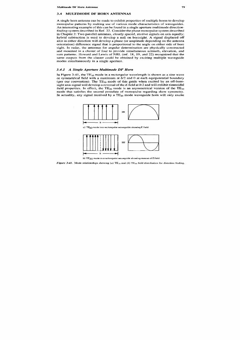
8/8/2019 SciTech - Microwave Passive Direction Finding
http://slidepdf.com/reader/full/scitech-microwave-passive-direction-finding 93/323
3.4 MULTIMODE DF HORN ANTENNAS
A single horn antenna can be made to exhibit properties of multiple horns to developmonopulse patterns by making use of various mode characteristics of waveguides.An interesting example of this can be found in a single aperture m ultimode direction-finding system described in Ref. 22 . Consider the phase m onopulse system describedin Chapter 2: Two parallel antennas, closely spaced, receive signals on axis equally;hybrid subtraction is used to develop a null on boresight. A signal displaced offaxis in either direction will develop a phase (or amplitude depending on the antennaorientation) difference signal that is proportional to the angle on either side of boresight. In radar, the antennas for angular determination are physically constructedand mounted in a cluster of four to provide simultaneous azimuth, elevation, andsum patterns. Howard and Lewis of NR L (ref. 18, 19 , and 22) recognized that thesame outputs from the cluster could be obtained by exciting multiple waveguidemodes simultaneously in a single aperture.
3.4.1 A Single Aperture Multimode DF Horn
In Figure 3-4 1, theTEJQ mode in a rectangular wavelength is shown as a sine wave
or symmetrical field with a maximum atb/2 and O at each equipotential boundary(per our convention). The TE20 mode of this guide when excited by an off-bore-sight axis signal w ill develop a reversal of theE field at b/2 and will exhibit sinusoidalfield properties. In effect, the TE2O mode is an asymmetrical version of the TEi0
mode that satisfies the second postulate of monopulse regarding skew symmetry.In actuality, any signal received by a TE2Q mode waveguide horn will only excite
G)TE|Qmode in a rectangular waveguide showing E field
b) TE 20 mode in a rectangular waveguide showing reverse of Efield
Figure 3-41. Mode relat ionships showing {a ) T E i 0 an d (b ) TE 2O field distribution for direction finding.

8/8/2019 SciTech - Microwave Passive Direction Finding
http://slidepdf.com/reader/full/scitech-microwave-passive-direction-finding 94/323
a nonzero output if it is off boresight and if each half of the mode is detected andsubtracted. The relationships between the modes are directly analogous to the patternrelationships required for monopulse systems. This was recognized by Howard (22)who constructed and described many variants of feeds using this principle. Anazimuth-elevation monopulse feed was built using the TE10 mode as a referencesignal (S), the TE2O mode as theH plane (A9), and a combination of the TEn andTM n modes to give theE plane difference (A^). The structure was built in a squarewaveguide (E = H)) to maintain the phase relationships of the modes. These moderelationships were transitioned into a single aperture horn antenna and used toprovide the standard monopulse feed network.
The advantage of the concept of mode-derived patterns is that excellent nullstability is attained since accuracy depends upon the properties of the mode excitationand support as a first-order effect as compared to factors in the construction, shapestability, and physical properties of direct radiators. Another advantage is the deriva-tion of the two ho rns ' monopu lse direction-finding properties from a simple radiatingfeed horn structure as compared to trying to match two different horns. Considera simplistic single plane (azimuth) version of a single-axis mode-derived horn
Dode detectors
Septum
Septum
Circuit connecton
Figure 3-42. Single axis waveguide horn DF system using mode separation techniques.
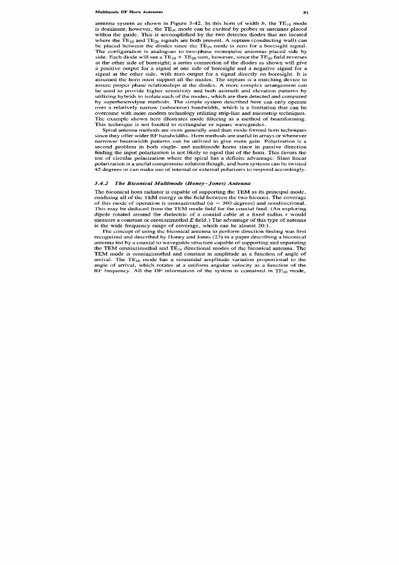
8/8/2019 SciTech - Microwave Passive Direction Finding
http://slidepdf.com/reader/full/scitech-microwave-passive-direction-finding 95/323
antenna system as shown in Figure 3-42. In this horn of widthb, the TE10 modeis dominant; however, the TE20 mode can be excited by probes or antennas placedwithin the guide. This is accomplished by the two detector diodes that are locatedwhere the TE10 and TE2O signals are both present. A septum (conducting wall) canbe placed between the diodes since the TE2O mode is zero for a boresight signal.The configuration is analogous to two-phase monopulse antennas placed side byside. Each diode will see a TE10 + TE2O sum, however, since the TE2O field reversesat the other side of boresight; a series connection of the diodes as shown will givea positive output for a signal at one side of boresight and a negative signal for asignal at the other side, with zero output for a signal directly on boresight. It isassumed the horn must support all the modes. The septum is a matching device toassure proper phase relationships at the diodes. A more complex arrangement canbe used to provide higher sensitivity and both azimuth and elevation patterns byutilizing hybrids to isolate each of the modes , which are then detected and com paredby superheterodyne methods. The simple system described here can only operateover a relatively narrow (suboctave) bandwidth, which is a limitation that can beovercome with more modern technology utilizing strip-line and microstrip techniques.The example shown here illustrates mode filtering as a method of beamforming.This technique is not limited to rectangular or square waveguides.
Spiral antenna methods are more generally used than mode-formed horn techniquessince they offer wider RF bandw idths. Horn methods are useful in arrays or whenevernarrower beamwidth patterns can be utilized to give more gain. Polarization is asecond problem in both single- and multimode horns since in passive directionfinding the input polarization is not likely to equal that of the horn. This favors theuse of circular polarization where the spiral has a definite advantage. Slant linearpolarization is a useful compromise solution though, and horn systems can be twisted45 degrees or can make use of internal or external polarizers to respond accordingly.
3.4.2 The Biconical Multimode (Honey-Jones) Antenna
The biconical horn radiator is capable of supporting the TEM as its principal mode,confining all of the TEM energy in the field between the two bicones. The coverageof this mode of operation is omniazimuthal (c|> = 360 degrees) and nondirectional.This may be deduced from the TEM mode field for the coaxial feed. (An exploringdipole rotated around the dielectric of a coaxial cable at a fixed radiusr wouldmeasure a constant or om niazimuthalE field.) The advantage of this type of antennais the wide frequency range of coverage, which can be almost 20:1.
The concept of using the biconical antenna to perform direction finding was firstrecognized and described by Honey and Jones (23) in a paper describing a biconicalantenna fed by a coaxial to waveguide structure capable of supporting and separatingthe TEM omniazimuthal and TE10 directional modes of the biconical antenna. TheTEM mode is omniazimuthal and constant in amplitude as a function of angle ofarrival. The TE10 mode has a sinusoidal amplitude variation proportional to theangle of arrival, which rotates at a uniform angular velocity as a function of theRF frequency. All the DF information of the system is contained in TEi0 mode,

8/8/2019 SciTech - Microwave Passive Direction Finding
http://slidepdf.com/reader/full/scitech-microwave-passive-direction-finding 96/323
either as an amplitude that varies with input angle or as an RF phase differencebetween it and the TEM mode. Two methods of extraction of the DF angle weredescribed: The first was a wide instantaneous video bandwidth video detectionsystem; the second a mode separation phase measurement superheterodyne tech-nique.
The original wideband video method used a coax-to-waveguide transition thatconverted the TEM and TE10 antenna modes into TEM and TE11 coaxial modes,
which were then further transitioned into four TE1Q ridged waveguide outputs, eachrepresenting a quarter, or 90 degree, view of the coaxial structure. Square lawdetectors placed at each waveguide port took the sum of the omniazimuthal andTE]1 components, detected them to remove phase differences, and then performedopposite pair subtraction to provide the resulting output video. This gave an outputsimilar to that of four orthogonally placed spiral antenna/detector combinations,except that the biconical beamwidths were mathematically 90 degrees wide andindependent of frequency, an optimum condition for a balanced system. Figure3-43 shows the essentials of the feed: A biconical antenna is fed by an overmodeduniform diameter coaxial structure capable of supporting the TEM and TEn modes.
Figure 3-43. Mechanical configuration of the biconical direction finder.
Waveguide detectoroutput ports
Section B-BWaveguidetransitionsection
Coax towaveguidetransitions
Coaxfilter
Section A-ACoax section
Biconicalantenna

8/8/2019 SciTech - Microwave Passive Direction Finding
http://slidepdf.com/reader/full/scitech-microwave-passive-direction-finding 97/323
An RF signal at a frequency where both modes are supported, arriving at an angle(J), establishes the TEM and the TE1 0 modes in the biconical antenna at that angle.These modes transition into the TEM and TE11 modes in the uniform length ofcoaxial line capable of sustaining them. At sectionB-B, a transition of each quarterof the coaxial cable into four TE10 waveguide outputs is gradually made. Figure3-44 shows the mode relationships along the signal path. The TEM mode movesrapidly from the antenna to the bottom of the coaxial structure, alternating in fielddirection. The TE10 mode of the antenna is bent and initiates the TE11 mode at theinput to the coaxial line at an angle proportional to$. The resultant energy travelsin two components that are orthogonal (of the form of the sine and cosine of (()).Propagation of this mode is spiral (like a circularly polarized wave) and is slowerthan the TEM mode, arriving at the bottom of the feed at a later time at an angle8, representing the phase (time) difference between the TEM and TE11 modes. Themaximum magnitude of the TE11 mode is directly proportional to the input angle$ rotated by as many degrees as required to travel the length of the coaxial line or"mode filter."
In the wideband DF system described by Honey-Jones, four VSWR-matcheddetectors were placed at each port providing outputs. The predetection signals areas follows:
Ex = A sin oof + B sin ((> sin((of - 8) (3-19)
E2 = A sin oof + B sin $ sin(oof - 8) (3-20)
E3 = A sin oof + B sin $ sin(oof - 8) (3-21)
E4 = A sin oaf + B sin $ sin(cof - 8) (3-22)
TEMMode TE10=TEN
Mode
Figure 3-44. Mode relationships in multimode biconical antenna and coaxial feed.
Cos <fi Sin*

8/8/2019 SciTech - Microwave Passive Direction Finding
http://slidepdf.com/reader/full/scitech-microwave-passive-direction-finding 98/323
where
A sin Mtcontains 1A of the TEM power
B sin § and B cos § = the two direction-carrying T E n mode signalssin(o)£ — 8) = the term containing 8, the phase lag between the TEM
and T E n modes
Detecting these signals provides four video outputs:
E \D = A2 + 2AB sin <> cos 8 + B 2 s i n2
< $ > (3-23)
E2D = A2 + 2AB sin c> cos 8 + B2 sin2 ()> (3-24)
£ 3 D = A2 + 2AB sin <> cos 8 + B2 sin2 <(> (3-25)
E4D = A2 + 2A £ sin cf> cos 8 + £2 sin2 <J) (3-26)An input signal will have twiceits power in the TEn mode as the TEM mode,hence B = 2A.
Examination of the detected equation set shows that each signal consistsof anangle-of-arrival term (the middle), which contains th e bearing information <$> thatvaries in output as a function of the phase lag (maximum output occursfor 8 = 0,the no lag case). By subtracting opposite detector pairs,sin <\> cos 8 and cos 4> cos8 terms containing all angle information unambiguously result.The subtractionprocess is necessary to develop unambiguous data, sinceth e presence of the cos 8creates a backlobe, which can equal the frontlobe when 8 = ir/2. Under theseconditions, the subtraction will causethe outputs to fall to zero. Cos 8, then, limits
the total bandwidth of the antenna by defining the operating range to be betweena fixed limit of output, 2 dB being chosen in the original reference. The coaxialmode filter is limited at the high-frequency end by the presence of a higher ordermode, the TE2I shown in Figure 3-45. This mode identifies itself as a variationappearing every 90 degrees.
T E 2 | Mode
Figure 3-45. The TE2,i higher order mode in the overmoded coaxial feed.

8/8/2019 SciTech - Microwave Passive Direction Finding
http://slidepdf.com/reader/full/scitech-microwave-passive-direction-finding 99/323
Figure 3-46. Subtracted output pairs of the ideal multimode biconical direction finder.
The original antenna covered 8 .3 -1 2 .4 GHz w ith peak errors ranging from ± 3to ± 7 degrees at the high-frequency end. The output patterns were sinusoidal infield as shown in Figure 3-46 and exhibited sharp DF video nulls of 21 dB. Thelimitations of this approach were clear; however, a long coaxial section desirableto attenuate the TE21 mode at the high-frequency end exacerbated the variation ofthe phase shift 8 causing the antenna output to fall. Detector matching and unequalsensitivities created additional errors. These problems led to the concept of separa-tion of the TEM, TEj1 sine, and TEn cosine modes through the use of quadraturecouplers and magic "T" hybrids. This technique led to several methods for DFdetermination that were unambiguous when using narrowband superheterodynetechniques to resolve phase ambiguities. The wideband methods were, unfortunately,ambiguous due to the inability to resolve the subtracted sine and cosine 180 degreesambiguity.
Later developments using the Honey-Jones antenna continued. An L-band su-perheterodyne direction finder utilizing the mode-separation filter technique wasdeveloped by Chubb, Grindon, and Venters (24). This system, shown in Figure3-47, utilized a turnstile junction and a series of hybrids, as shown, to form threeoutput voltages:
Vx = AA cos oof (3-27)
which is the TEM omniazimuthal signal
V2 = IB COS(Wf + <|>) (3-28)
Pdir I
Pair 2 Pair 2
Pair I =Cos <f>
Pair 2 = Sin <f>
Pair I

8/8/2019 SciTech - Microwave Passive Direction Finding
http://slidepdf.com/reader/full/scitech-microwave-passive-direction-finding 100/323
Figure 3-47. Narrow band superheterodyne phase monopulse direction finder (after Ref. 24, Chubbet al.).
the TEn right-hand circularly polarized component and
V3 = IB cos(cot - (J)) (3-29)
the TE11 left-hand circularly polarized component.
To process these signals, a modified version of a three-channel class III processorwas used, with an additional 90 degree preprocessing phase shift added.
By examination, it can be seen that only the V1 and either of V2 or V3 need beused to obtain 4>; how ever, the system was used to detect moving aircraft, whichcreate multipath interferences that continually change. By measuring§ using V1
and V3 and averaging the results, the multipath component can be made to cancel.The resultant improvement in accuracy was substantial (about 6:1), w ith a final
Sn <>
Cos <f>ThreeChanneClassm
SuperheterodyneProcessor
PhaseShift

8/8/2019 SciTech - Microwave Passive Direction Finding
http://slidepdf.com/reader/full/scitech-microwave-passive-direction-finding 101/323
error of approximately 5 degrees RMS. The signals V1, V2 > and V3 were phasedcompared to V1 to determine 4>. The phase dispersion 8 between the TEM and TEnmodes must be subtracted out, which required a knowledge of frequency that wasnot difficult here since detection was at a known beacon frequency. The TE21problem was not encountered since operation was below the frequency at whichthis mode appeared. Although partially suited to the objectives of wideband passivedirection finding, the above system worked with cooperating aircraft as part of acollision avoidance technique to demonstrate feasibility. For wide RF bandwidth,a scanning superheterodyne receiver could give frequency information for postdetec-tion 8 compensation that would permit the receiver to scan over a suboctave range.
A wider RF bandwidth antenna system had been envisioned by Honey but wasnot achieved until two important facts were realized: Mode separation and cancel-lation of the TE2I m ode could be achieved by proper design of a hybrid feed networkand the phase delay between the coaxial TEM mode and the waveguide TE11 modescould be compensated for prior to detection. In addition, better methods could bedeveloped to extract the various modes by utilizing turnstile RF mode techniquesas undertaken by Chubb et al. (24).
The Honey-Jones antenna has always been attractive for direction finding becauseof the symmetry of its design and the natural circular phase front exhibited by the
bicone. It is also possible to provide an elevation(H plane) tilt for above the horizonapplications to minimize ground clutter. This better control of elevation is a prominentreason for its continuing development.
The original Honey-Jones antenna was a four-port device; that is, there werefour RF outpu ts, each containing the sum of the TEM and TE11 modes. These weredeveloped by a transition of the coaxial feed to waveguide. A later approachconsidered the use of five ports. The first was a standard coaxial output mountedat the bottom of the feed to extract the TEM or omniazimuthal mode directly. The
others consisted of four orthogonally spaced coaxial probes whose isolated centerconductor intercepted the dielectric of the coaxial feed network, m uch as an antennawould. These four probes lay in a plane perpendicular to the direction of the feedand were spaced 90 degrees around the circumference. Figure 3-48 is a diagramof the arrangem ent. The five-port device effectively formed a turnstile junction withthe advantage of a separate omniazimuthal output. This permitted a wide openazimuthal coverage for other purposes such as instantaneous frequency measure-ment, while the four DF ports could be used for direction-of-arrival determination
on a pulse-by-pulse basis.Although the above described antenna was built and fulfilled its design objectives,
it became evident that the separation of the modes indirectly, by a hybrid excitationmatrix, could provide the TEM output and offer additional advantages. Since thisis perhaps the most significant configuration of the Honey-Jones concept, it willbe explained in more detail. Figure 3-49 shows the approach. Four TE11 probesreceive the energy that has propagated down the coaxial filter connected to themultimode bicone antenna. Each p robe will detect the sum of the TEM com ponent,the TE11 value, and the undesired TE21 mode, assuming operation for the worstcase frequency where all modes occur. There will also be a phase angle 8 representing

8/8/2019 SciTech - Microwave Passive Direction Finding
http://slidepdf.com/reader/full/scitech-microwave-passive-direction-finding 102/323
Figure 3-49. Three-port wideband Honey antenna system with TE2I mode canceled.
Phaseshifter
Figure 3-48. Five-port turnstile biconical antenna feed with mode separation.
Dielectric
Coaxprobe
Section X-XT EN Coaxialprobes intodielectric
TEMProbe
at base
Feedstructure
Air o r foamdielectric
Innerconductor
Outerconductor
TE|(
Probes1-4
Biconicalcoaxialfeed

8/8/2019 SciTech - Microwave Passive Direction Finding
http://slidepdf.com/reader/full/scitech-microwave-passive-direction-finding 103/323
the delay in propagation of the TE11 and TEM m odes . Hybrids 1 and 2 are connectedto alternate probes and provide the sum and the difference output of the signals.This is done at a loss of 3 dB in power or a .707 (V2/2) in voltage since 3 dBhybrids are used. The sum (X) outputs OfZZ1 and Hi are combined inZZ3 and appearat the sum (2 ) port of ZZ3 as a cos u>t term. This output is delayed in a phase shifterwith a phase angle 8 to compensate for the faster propagation of this mode downthe overmoded coaxial filters. (The phase shifter is actually a piece of waveguideexhibiting both the delay and frequency dispersion characteristics of the antennafeed structure.) The final output at port 2 is of the form cos (atf + 8), which isseen to be the omniazimuthal TEM mode of the antenna. The proof of this iscomplex; a simplified method will be used for understandability.
Consider Figure 3-50, which shows the polarity of a voltage of unity inducedin each of the probes for each of the modes of propagation, the TEM, TE11, sine,TE11 cosine, and TE21. The convention used here is that the field will induce anegative polarity when it is in the same direction as the probe and will induce novoltage (shown for the TE11 case) when it is orthogonal or perpendicular to theprobe. Since the antenna is a linear device, the law of superposition holds and eachmode can be analyzed separately. Since the fields are symm etrical, it will be assum edthat equal voltages are induced at opposite ports. Reexamining Figure 3-49 for the
TEM mode, probes P3 and P1 are fed to Hi, and P2 and P4 are fed to H1. The
a) TEM mode probes b)TE|| Cos mode
c) TE11 Sinmode d) TE2,probes
Figure 3-50. Polarities of the E field induced the probes for each of the three modes present at thebottom of the coaxial feed (E pointed IN is negative), (a) TEM mode probes, (b) TEn cos mode, (c)TEn sin mode, (d) TE2I probes.

8/8/2019 SciTech - Microwave Passive Direction Finding
http://slidepdf.com/reader/full/scitech-microwave-passive-direction-finding 104/323
polarity of the induced voltages in each probe is - 1 ; therefore at the differenceports of each hybrid, there will be 0 TEM V and at each sum port, there will be- 1 . 4 1 4 (2X - V2/2 of each input) V. At hybridH3, the difference port will have0 TEM V, and the sum port will have the sum of all four ports or -2.28(y/2J2)V. The result is that hybridHx has separated out the cosine component of the TEnmode. By similar reasoning, hybridH2 separates out the sine component of theTE11 mode. The final output voltage of each m ode is shown at port 1 to be sin§cos(co/ + 6) and at port 3 to equal cosfy cos((ot+ 8).
The TE21 mode analysis is interesting: At the A port OfZZ1 the TE21 mode cancels,and at the E port -1.414 TE21 V is present. AtH2, cancellation again occurs forthe TE21 mode, at the A port leaving +1.414 TE21 V at the E port. When the two
TE21 V are combined inH
3,
they cancel and are terminated in the load placed atthe A port. All TE21 energy has therefore been removed by the feed matrix, andthe effects of the TE21 mode disappear. The S port ofH3 contains only the TEMsignal. This is a significant consequence since the antenna can now operate beyondthe previously limiting upper frequency. The second limitation has been alreadyminimized by the addition of the 8 filter in the TEM mode; comparison of the threeoutputs are now all in phase. The result of this feed method permits the antennato achieve full octave coverage by connection to a superheterodyne three-channel
class II processor (logarithmic amplifiers with detectors and subtractors) to formthe tan $ or cot c> amplitude ra tio. This removes the cos(a)f + 8) term in thedetection process. By noting if sine is greater than cosine, division by zero can beavoided and the appropriate tangent or cotangent output is used. Figure 3-51 is a
Figure 3-51. Three-output Honey-Jones antenna and polarizer. Courtesy of SRI International.

8/8/2019 SciTech - Microwave Passive Direction Finding
http://slidepdf.com/reader/full/scitech-microwave-passive-direction-finding 105/323
Figure 3-52. Recombination network for four-quadrant square law detector output.
version of the antenna that has the three outputs described above, as was used withthe class II processor. Since the biconical antenna is vertically polarized, the figureshows it mounted within a "meander line" polarizer permitting reception of hori-zontal, vertical, and circular polarization.
The direction finder described above, although offering wide RF bandwidth,requires the class II processor, which is a superheterodyne receiver w ith logarithmicIF amplifiers. This processor provides linear detection due to the high-gain, high-level detection process and, invariably, is a relatively narrow band, requiring afrequency scanning process to explore a frequency range.
The original concept of a broadband square law detected system can be realizedby expansion of the three-hybrid network back into a four-output network. Thismay be done by recombination of the three modes with three additional hybrids asshown in Figure 3-52. The omniazimuthal signal, devoid of its phase difference,is split and fed to hybridsH4 and H5. Each hybrid also received either the TE11
sine or cosine signal. By analogous reasoning it may be shown that four outputsare obtained:
cos((of + S)(A - Bsin <|>) (3-30)
cos((of + 8)(A 4- B sin c|>) (3-31)
cos(o)f + 8)(A - B cos cf>) (3-32)cos(cof + 8)(A + B cos ()>) (3-33)
Powersplitter

8/8/2019 SciTech - Microwave Passive Direction Finding
http://slidepdf.com/reader/full/scitech-microwave-passive-direction-finding 106/323
Figure 3-53. Broadband Honey antenna with multiport strip-line feed network. Courtesy of SRI International.
The TE2I mode is canceled out by elimination in the A port of hybridH3 inFigure 3-49. The output of the system still is multiplied by cos 8, bu t thedispersionwith frequency has been reduced to the extent that the equalizer can replicate theovermoded coaxial line dispersion. This is important since, in linear detector systems,the loss due to the dispersion affects ambiguity resolution. In quadratric systems,reductions of the dispersion permits a wider bandwidth for a given 8. In general,
8 is nonzero in the overmoded line since a finite length must be used, which musthave some value since it is not feasible generally to make it zero.
The structure of a complete hybrid-equalized quadratic detected antenna systemis shown in Figure 3-53, a photograph of the bottom of the antenna. The feednetwork utilizes wide bandwidth strip-line couplers to provide equal power splitswith excellent phase tracking . The biconical antenna is filled with a poly foamstructure to support a mode suppressor to eliminate any spurious horizontal response.
3.5 ROTATING RE FL EC TO R AN TE NN AS
The rotating passive reflector type of antenna still finds wide application in DFsystems due to its simplicity and potential for reasonable gain with good backloberesponse. The effective aperture of a rotating reflector, however, is never that ofthe reflector area alone since there is an illumination efficiency associated with theprocess. This efficiency is dependent upon the shape of the taper of the beam ofthe illuminating antenna and the reflectivity.

8/8/2019 SciTech - Microwave Passive Direction Finding
http://slidepdf.com/reader/full/scitech-microwave-passive-direction-finding 107/323
An antenna such as a spiral or a horn can be rotated directly by feeding it througha mechanical rotary join t. This is sometimes done ; how ever, it is not always possibleto achieve the front-to-back-lobe ratios of a reflector since two additional degreesof control are provided: the shaping or focusing of the passive reflector to increasegain and the ability to adjust the illumination or taper of the radiating structure tooptimize the beam shape and back-lobe response. Rotating antennas, however, arestill used. Multiple-channel rotating DF systems have been built using sum(Z) anddifference (A) channels in multiple-channel rotary joints , often in narrow R F band-width radar applications. For wide RF bandwidth systems, as required in passiveDF applications, however, direct rotating radiators are generally limited.
There are many approaches to rotating reflector antennas. If a simple flat platepassive reflector is rotated at an angle above a linearly polarized feed, the polarizationwill rotate with the reflector and become a function of pointing angle. For thisreason, most rotating reflectors use circularly polarized feeds or rotate the antennaand the reflector as a unit, using an RF rotary joint to make connection to theantenna. This is possible at frequencies where a good rotating antenna can be built.Since most rotary joints are coaxial, it is necessary, for mechanical reasons, to goto a TEM or coaxial type of transmission line at the joint assembly. For mostapplications, this limits the frequency range to bands where coaxial line can beused, placing the upper limit at approximately 20 GHz.
It has almost always been an object in the design of a rotating reflector systemto shape the resultant pattern so that it can exhibit fan beam charac teristics. A notherobject at high frequencies has been to shape both the vertical and horizontal beam-widths into a narrow "pencil beam " for high gain, especially at very high frequencies(above 20 GH z), to attempt to overcome transmission path propagation losses. Thesmaller size of the reflectors at these higher frequencies is a tempting prospect;however, the need for a circularly polarized feed imposes a practical limitation.
We shall consider both problems and cite examples of successful implementationsof both techniques.
3.5.1 A Broadband Shaped Beam Rotating DF System
The early concepts for the design of a shaped reflector system go back as far as1946, when Stavis and Dome described horn illuminated elliptical paraboloid reflectors(25). The conclusions reached are shown in Figure 3-54. A reflector shaped elliptically
in elevation will yield a fan or broad-beam pattern (usually shaped as a cosecant2
//-plane pattern); a parabolic shape in azimuth will narrow the azimuthal beam.Other conclusions are that a circular polarized feed is required to provide constantillumination of the reflector and that the horn pattern must be symmetrical aboutthe horn axis . Baffles were found experimentally to reduce the size of the horizontalreflector surface.
Work was undertaken at American Electronic Laboratories to develop a rotatingDF antenna with a wide (2-18 GHz) RF bandwidth, a constant beamwidth, and awide H plane (0) pattern to permit predictable DF processing algorithms to be usedfor shipboard use. This work was described by Bohlman (26). Figure 3-55 shows

8/8/2019 SciTech - Microwave Passive Direction Finding
http://slidepdf.com/reader/full/scitech-microwave-passive-direction-finding 108/323
Top view
Figure 3-54. Shape of a focused reflector for a narrow azimuthal (<|>) and wide elevation (0) beam.
Q= Horizontalaperture(parabolic)
Side view
Radiating horn
AA
b= Vertical aperture(elliptical)

8/8/2019 SciTech - Microwave Passive Direction Finding
http://slidepdf.com/reader/full/scitech-microwave-passive-direction-finding 109/323
Figure 3-55. A 2-18 GHz rotating DF system using a shaped passive reflector. Courtesy of AEL.
the design. A broadband 2» 18 GHz circularly polarized spiral antenna is mountedat the com mon focus of a reflector designed to be parabolic in azimuth and ellipticalin elevation. The spiral illuminates the reflector and is rotated with it through a2 - 1 8 GHz rotary joint to eliminate pattern m odulation due to the rotation and reducesquint. The reflector is 16 by 14 inches in size across these two curves. The ellipse
that forms the azimuth beam has a second focus designed to minimize the apertureblockage due to the presence of the radiating spiral by placing it in front of theaxis of rotation and 8 inches above the feed. Moving this focus point further outnarrows the elevation beamwidth since the design of the elliptical section of thereflector will approach a parabola for widely separate foci. In the case of this design ,a full fan beam was not desired in favor of increased gain. The reflector is constructedof laminated fiberglass sheets, honeycomb supported for added strength. The con-ducting surface is plated with a thin coating of silver coated with polyurethane to
prevent oxidation. Absorber material is judiciously positioned to reduce reflectors.The bearing shaft of the reflector supports the rotary joint.
The feed antenna is a 2.3 inch circularly polarized cavity-backed archimedianspiral of fairly straightforward design. The radiation characteristic of this antennais such that the beamwidth increases at the 2 GHz low frequency, which wouldtend to overilluminate the reflector, creating undesired backlobes. Since the reflec-tor is parabolic in azimuth, this beam narrows; however, the elevation pattern inelevation increases. This may be seen in Figure3-56a, which shows the azimuthbeamwidth increasing to 23 degrees from a 5 degree average value over most ofthe band. The figure also shows the excellent axial ratio of this approach. Figure

8/8/2019 SciTech - Microwave Passive Direction Finding
http://slidepdf.com/reader/full/scitech-microwave-passive-direction-finding 110/323
Frequency (GHz)b)Eevaton ange measured at - 6dbdown from beam peak
Figure 3-56. Rotating reflector antenna beamwidth.(a ) Azimuth RF beamwidth. (b) Elevation anglemeasured at —6 dB down from beam peak.
3-56b shows the elevation for the 6 dB down off-peak beam gain, which increasesat the lower-frequency end. The gain of the antenna and the boresight pointingerror are shown in Figure 3-57a andb. Gain rolloff at the low end mirrors theincrease in antenna beamwidth and efficiency of the spiral. The beam tilt is relatedto the sense of the circular polarization, the reflector size, and the feed offset (27,2 8 ) . A trade-off was made in this design between a fixed antenna mounted at theaxis of rotation and the use of an offset feed and rotary joint. It was anticipatedthat the low-end beam variation would have caused a 10 degree beam tilt at 2 GHz
Below
horzon
H
orz.
Ab
ove horzon
a)AzmuthRFbeamwidthFrequency (GHz)
3db azim
uth beam
w
idth
°

8/8/2019 SciTech - Microwave Passive Direction Finding
http://slidepdf.com/reader/full/scitech-microwave-passive-direction-finding 111/323
with the fixed antenna, compared to the 3 degrees attained here. The final antenna,which is mounted in a full radome, sweeps a volume 22 inches in diameter by 16inches in height. It provides an azimuth beamw idth of approximately 2 .5 -2 3 degreesover an //-pla ne 6 dB beamw idth of + 2 0 degrees above to - 5 degrees below thehorizon. The front-to-back and all other lobe ratios are - 2 0 dB down at all frequencies.
In another reflector-type antenna, the reflector was designed to provide a 1.5 x2 degree pencil beam that could provide a narrow high scan. This required that thereflector be able to rotate in azimuth and scan in elevation. Figure 3-58 shows thisantenna, which covers the 10-40 GHz range in three bands. The illuminatingelements are three fixed circular polarized horns mounted as close to the axis ofrotation as possible. The reflector rotates on a slip assembly that carries the circuitassociated with the tilting mechanism. The reflector is a flame-sprayed conducting
G
ain(dbi)
Frequency (GHz)a) Gan
Frequency (GHz)b) Boresightpontng error
Figure 3-57. Rotating reflector antenna (a) gain and (b) boresight pointing error.
To
p view
M
B
CW
.
C
C
W
.

8/8/2019 SciTech - Microwave Passive Direction Finding
http://slidepdf.com/reader/full/scitech-microwave-passive-direction-finding 112/323
Figure 3-58. Two axis shaped reflector scanning antenna.
fiberglass design with baffles that develop the required pencil beam at gain levelsof approximately 35 dB. Dual servo systems provide the two axes of rotation.
3 .6 SUMMARY
Chapter 3 presented the most popular types of antennas in current use for passivedirection finding. It is not always clear why a certain design or system has beenchosen, so emphasis has been placed on the key features of the designs. The actualantenna choice will generally be dictated by the system, the required accuracies,and the cost.
A DF system can almost be made as accurate as desired if sufficient antennaaperture is available. The driving factors, however, are the available geography forthe DF system, the host vehicle requirements, and the mission needs. For simpledetermination of locations, line of bearing accuracies of 8-10 degrees peak are
usually good. For targeting or aiming, accuracies of better than 2 degrees arerequired . For high-gain electronic countermeasures (ECM) or jam m ing , fractionalaccuracies are needed. In these cases the accuracy must be developed by signal

8/8/2019 SciTech - Microwave Passive Direction Finding
http://slidepdf.com/reader/full/scitech-microwave-passive-direction-finding 113/323
processing both by analytical means and by digital or processing means. We shallstudy both methods in the chapters that follow.
R E F E R E N C E S
1. "IEEE Standard Test Procedures for Antennas," Antenna Standards Committee, ANSI Institute ofElectrical and Electronics Engineers: New York, Wiley, 1979.
2. Turner, E., "Spiral Slot Antenna," U.S. Patent 2,863,145, Dec. 1958.
3. Booker, H. G., "Slot Aerials and Their Relation to Complementary Wire Aerials,"Journal Instituteof Electrical Engineering, Pt. HIA, 1946, pp. 620 ff.
4. Kaiser, J. A. , "The Archemedian Two-W ire Spiral Ante nna,"IRE Transaction AP-8,1960, p. 313 .
5. Rumsey, V. H., Frequency Independent Antennas,New York: Academic Press, 1966.
6. Dyson, J., "The Unidirectional Equiangular Spiral Antenna,"IRE Transaction AP-7,Oct. 1959.
7. DuHammel, R. H., and D. E. Isbell, "Broadband Logarithmically Periodic Antenna Structures,"IRE Intern. Conv. Record, 1957, pp. 119 ff.
8. Marchand, N., "Transmission-Line Conversion,"Electronics, Dec. 1944, pp. 142 ff.
9. McL aughlin, J., D . Dunn , and R. Grow, "A Wide-Band Balum ,"IRE Transactions on MicrowaveTheory and Techniques, July 1958, pp. 314 ff.
10. Stutzman, W., and G. A. Thiele,Antenna Theory and Design,New York: Wiley, 1981, p. 283.
11. "Antennas, Masts, Mounts and Adapters,"AEL Catalog7827.5M, American Electronic Laboratories,Lansdale, PA, 1982, p. 46.
12. Hahn, G., and R. Honda, "Conical Spiral Arrays for Passive Direction Finding,"USAF AntennaSymposium Proceedings,Allerton Park, Monticello, IL, Oct. 1968.
13 . Kaiser, J., H. Smith, W. Pepper, and J. Little, "A Passive Automatic Direction Finder,"Proc. IRE9th ECCANE,Baltimore, MD, Oct. 1962.
14. Dyson, J., "The Equiangular Spiral Antenna," University of Illinois Antenna Laboratory, ReportNo. 21, Apr. 1955.
15 . Chadwick, G., "Multiple Arm Spiral and Its Derivatives for DF and Homing," Presented at LosAngeles IRR Group on Antennas and Propagation, Jan. 15, 1970.
16. Lantz, P., "A Two-Channel Monopulse Reflector Antenna System with a Multimode LogarithmicSpiral Feed," Presented at the 16th Annual USA F Symposium on Antenna R& D, R adiation S ystems,Inc., Report, NASA Contract NAS5-9788, Oct. 1966.
17 . Chadwick, G., and J. Shelton, "Two Channel Monopulse Techniques—Theory and Practice,"International Convention on Military Electronics, Sept. 1965.
18. Lipsky, E., "The Antector, a Millimeter Wave Spiral Detecting Antenna," Presented at the 3rdAnnual Benjamin Franklin Symposium, IEEE MTT&AP Societies, Philadelphia, PA, April 1983.
19. Skolnik, M., Ed., Radar Handbook,New York: McGraw-Hill, Chap. 8.20. Hopfer, S., "The Design of Ridged Waveguides,"IRE Transactions-MTT,Oct. 1955, pp. 20 ff.
21. Jasik, H., Ed., Antenna Engineering Handbook,New York: McGraw-Hill, 1961, pp. 1 0 - 1 3 .
22. Howard, D., "Single Aperture Monopulse Radar Multi-Mode Antenna Feed and Homing Device,"IEEE International Con vention on Military Electronics, Washington, D . C , 1964.
23. Honey, R., and E. M. T. Jones, "A Versatile Multiport Biconical Antenna,"Proceedings of IRE,Vol. 45, No. 10, Oct. 1957.
24. Chubb, E., J. Grindon, and D. Venters, "Omnidirectional Instantaneous Direction Finding System,"
IEEE Transactions on Aerospace and Electronic Systems, Vol. AES-3, No. 2, March 1967.25. Radio Research Laboratory, Harvard UniversityStaff, Very High Frequency Techniques,New York:
McGraw-Hill, 1947, Vol. I, p. 164.

8/8/2019 SciTech - Microwave Passive Direction Finding
http://slidepdf.com/reader/full/scitech-microwave-passive-direction-finding 114/323
26. Bohlman, W., "Broadband Rotatable Direction Finding,"Antenna AP-S International SymposiumDigest, 1977, p. 104.
27. Lu h, H., and A. Tsa o, "Null Shift and Beam Squint in Circularly Polarized Offset-ReflectorAntenna," IEEE Transaction AP-34,Jan. 1986, p. 97.
28. Chu and Turrin, "Depolarization Properties of Offset Reflector Antennas,"IEEE Transaction AP-27, May 1973, p. 339.
Note\ The above list of references in antenna technology constitute only a small part of the availableantenna literature. The author wishes to apologize to those not listed; the reader will find additionalsource material in the listing of references by the above authors.

8/8/2019 SciTech - Microwave Passive Direction Finding
http://slidepdf.com/reader/full/scitech-microwave-passive-direction-finding 115/323
DF ReceiverConfigurations
In this chapter, passive DF systems used for radar warning and ELINT purposeswill be described in terms of the DF concepts and antenna technologies presentedthus far. System configurations typical of present-day implementations will bedetailed in various generic block diagrams. In each case, the reader should identifythe type of system and, if monopulse, determine the class and method of satisfyingthe criteria for angle extraction. This recognition process will develop an appreciationof the potential a given system has to attain specific goals. Some systems aredesigned for warning, some for data gathering, and some for high accuracy; in eachcase, a specific design offers advantages and disadvantages. A wide instantaneous
bandwidth receiver may be readily jammed; a narrow bandwidth system will losedata but may be more accurate measuring the data it does process. It is hoped thatby following these rules, the reader will develop an insight into system "entropy,"or overall capability to achieve a desired objective.
4.1 DF RADAR WARNING RECEIVERS
In the microwave region, angle-of-arrival data is used primarily as a means ofdetermining the line-of-bearing of a signal or the position of an emitter with respectto either the DF host vehicle or the overall situational geography. The first case isusually for threat warning, where the identification, direction, and rate of closureare important factors for self-protection. The second case is for electronic order ofbattle (EOB) for the purposes of calibrating the signal environment, to determinethe circle of error probability (CEP) or location, to recognize changes in the presenceof known static situation, or the initiation of a new threat cond ition. We have studied
the rotating DF system utilizing skirt-inhibition and its evolution td monopulse,which, because of its capability for high accuracy, addressed the EOB problem.
Chapter Four

8/8/2019 SciTech - Microwave Passive Direction Finding
http://slidepdf.com/reader/full/scitech-microwave-passive-direction-finding 116/323
This has led to the study of monopulse theory as utilized in radar. To show theapplication of the theory to passive DF systems, it will be useful to study one ofthe most popular applications, that of the radar warning receiver (RWR).
Threat warning applications are characterized by the need for wide open frequencyand angular coverage, rapid identification for determination of threat status, andDF information for se lf-protection. Figure 4-1 is a diagram of what we shall defineas a generic radar threat warning receiver (1 -4 ) . It is a four-antenna system utilizingwide beamwidth, wide bandwidth spiral antennas to provide high probability ofintercept over a typical 2-18 GHz frequency band.
Four antennas geographically dispersed about the host vehicle provide four angularquadrants of coverage of 360 degrees of azimuth. The type of antenna used for thisapplication m ust have essentially no backlobes and must exhibit antenna beamw idthsof approximately 90 degrees to achieve 360 degree omniazimuthal coverage. Planarcavity-backed spiral antennas, as discussed previously, closely exhibit these propertiesand for this reason are most commonly used in RWR applications. The idealizedpatterns of four such spirals is shown in Figure 4-2. Although these patterns varyin 3 dB beamwidth, from 70 degrees at 18 GHz to approximately 100 degrees at2 GHz, full 360 degree coverage is provided unam biguously, with sufficient articulationto make measurements. The angle of arrival (J) of an input signal measured from
boresight by the receiver corresponds exactly to the case of an amplitude monopulsesystem as defined previously for the equivalent radar case. Since the beamwidthsare wide as compared to radar, the accuracies and resolution are correspondinglypoorer (typical values lie between 5 and 10 degrees). The formation of the am plitudemonopulse ratio requires determination of the strongest and next adjacent strongestsignals, shown in Figure 4-2 asVA and VB, a process easily implemented in fastparallel logic. Since the antenna output is RF signal energy, the receiver must bein close proximity to reduce losses, especially at the high end of the 2-18 GHz
band. Each antenna is therefore connected to a receiver, or a dual receiver canservice two antennas if the RF cable runs are short, as is the case in wing-tip orhelicopter installations. Detection of the signal takes place for the frequency rangein one band, or the detector may be preceded by a band separation multiplexer,which divides the band into sectors. Figure 4-3 shows these various possibilities.In Figure 4-3a, the entire 2-18 GHz band is detected and logarithmic amplifiedfor each antenna. A diode limiter precedes the detector (shown for all cases) toprevent burnout at high signal illumination levels. This configuration gives the
maximum intercept probability but suffers most from the possibility of pulse overlapor continuous wave (CW) problems in a dense signal environment, since no reductionof data by frequency band selection is possible. In Figure 4-3&, each of the fourantennas is connected to a quadraplex filter, which divides the original 2-18 GHzband into sub-bands, each of which is detected and logarithmically amplified. Thisconfiguration provides the maximum probability of intercept and the feature offrequency band information as a result of the multiplexing. It is, unfortunately, themost expensive and complex, with 16 video signals to be handled by the bearing
computer. The data rate is high but can be reduced by sampling the 16 outputs ona band-by-band basis. This switching can also be used to sample or "chop" CW

8/8/2019 SciTech - Microwave Passive Direction Finding
http://slidepdf.com/reader/full/scitech-microwave-passive-direction-finding 117/323
Figure 4-1. Generic warning receiver
Ampliencod
DFvideo
DigitalD F
DFcomputer
Interceptmemory
Associativeprocessor
(sorts signals)
a - p r i o r ifile
4 Logv ideooutputs ignals
R e c e i v e r
D F antenna system
Band select
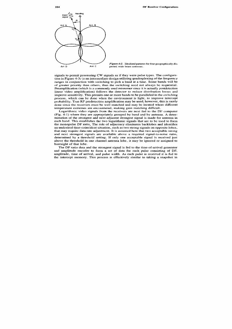
8/8/2019 SciTech - Microwave Passive Direction Finding
http://slidepdf.com/reader/full/scitech-microwave-passive-direction-finding 118/323
signals to permit processing CW signals as if they were pulse types. The configura-tion in Figure 4-3c is an intermediate design utilizing quadraplexing of the frequencyranges in conjunction with switching to pick a band at a time. Some bands will beof greater priority than others, thus the switching need not always be sequential.Preamplification (which is a commonly used misnomer since it is actually postdetectionlinear video amplification) follows the detector to reduce distribution losses andimprove sensitivity. This permits one or more bands to be paralleled in the switchingprocess, which can be done when the environment is light, to improve intercept
probability. True R F predetection amplification may be used; however, this is rarelydone since the receivers must be well matched and may be located where differenttemperature extremes are encountered, making gain matching difficult.
Logarithmic video signals from the receivers are next fed to the DF computer(Fig. 4-1) where they are appropriately grouped by band and by antenna. A deter-mination of the strongest and next adjacent strongest signal is made for antenna ineach band. This establishes the two logarithmic signals that are to be used to formthe monopulse DF ratio; The rule of adjacency eliminates backlobes and identifies
an undesired time-coincident situation, such as two strong signals on opposite lobes ,that may require data rate adjustment. It is assumed here that two acceptable strongand next strongest signals are available above a required signal-to-noise ratio,determined by a threshold setting. If only one acceptable signal is received justabove the threshold in one channel antenna lobe, it may be ignored or assigned toboresight of that lobe.
The D F ratio data and the strongest signal is fed to the time-of-arrival generatorand amplitude encoder to form a set of data for each pulse consisting of DF,amplitude, time of arrival, and pulse width. As each pulse is received it is fed tothe intercept memory. This process is effectively similar to taking a snapshot in
Ant D Ant CFigure 4-2. Idealized patterns for four geographically dis-persed wide beam antennas.
HeadingInputsignal
Ant A Ant B

8/8/2019 SciTech - Microwave Passive Direction Finding
http://slidepdf.com/reader/full/scitech-microwave-passive-direction-finding 119/323
time of the signal environment with the exposure time analogous to the time (capacity)to fill the memory. When the memory is full, the encoded signals are either ignoredor fed to another parallel memory until the first time snapshot is processed. Thisprocessing is accomplished in non-real time to deinterleave the pulse by separatingthem into pulse trains, after which they are compared to an a priori memory foridentification. A look-up table provides DF correction as a function of band orazimuth if calibration data is available.
The result of the processes described above is a prioritized threat file that isdisplayed to the operator on a threat display. This is usually a polar CRT plot ofsignal type versus angle of arrival at range of imminency or danger, based uponsignal strength, lack of scan, constant illumination, or identification with a priori
data. After a cycle of processing, the intercept memory is cleared, the process
Geographicalydspersed antennas
Wdebandlog vdeooutputs
a- Smpe wde open recever
b-Parallelmutpexed receiver
Multplexedlog vdeooutputs
Swchedmultplexedlog vdeooutputs
Figure 4-3. Various warning receiver front en ds,(a) Simple w ide open receiver,(b) Parallel multiplexedreceiver, (c) Switched multiplexed receiver.
c-Switched multiplexed receiver

8/8/2019 SciTech - Microwave Passive Direction Finding
http://slidepdf.com/reader/full/scitech-microwave-passive-direction-finding 120/323
repeats itself, and the display is refreshed. The simpler generic radar warningreceiver described above is defined as DF driven; that is, decisions are made onthe basis of DF and pulse-time information. Frequency data, if available at all, isonly on a band-by-band basis. Since arriving signals vary in strength, the monopulsesignal-to-noise ratio may vary in amplitude. This may degrade the quality of theDF measurement, and care must be taken to select an operating threshold for thesystem that prevents a single signal from falsely appearing at several DF angles.If a signal becomes strong enough to overload the receiver, it can cause the DFmeasurement to vary again with the same result. For this reason, high DF accuracyand large dynamic ranges are necessary. This has been accomplished in recent yearsby improved detectors and video logarithmic amplifiers.
Figure 4-4 is a photograph of the APR-39A (XE-I) radar warning receiver,manufactured by the Dalmo Victor Division of the Singer Corporation, illustratingthe mechanical configuration of a helicopter-mounted high-performance receiverutilizing special antennas and receivers, manufactured by American Electronic Lab-oratories, to cover frequency ranges extending from the H through M bands (5).Figure 4-5 is a photograph of another high-technology radar warning receiver, theGeneral Instrument model AN /ALR -80, which also illustrates advanced RW R tech-nology (6 ). In the AN /ALR-80 four spiral antennas that are geographically dispersed
about an aircraft feed four receivers (shown in the center), each of which , in parallel,detects and amplifies the DF signals feeding them to the digital signal processor(far right). Here a complex computer capable of 1.2 x 10⁶ operations per seconddetermines the monopulse DF and associates signals to permit their identificationagainst a directory of over 1000 known signals stored in an electronic erasableprogrammable memory (EEPROM). This data bank can be preflight updated in 90seconds at a flight-line to accept different environments. Fifteen emitters of thehighest priority are displayed on the digital display indicator (upper left) as alphanumeric
symbols, designating the class of signal (friend, foe, or unknown) and the range
Figure 4-4. The APR -39A (X E-I ) radar warning receiver. Courtesy of Dalm o Victor, Division of SingerCorp.

8/8/2019 SciTech - Microwave Passive Direction Finding
http://slidepdf.com/reader/full/scitech-microwave-passive-direction-finding 121/323
Figure 4-5. The AN /ALR -80 radar warning receiver. Courtesy of General Instrument Co rp., G overnmentSystems Division.
and DF bearing of each. The information is presented by placing the interceptsymbol at a distance from the origin as a function of threat priority at the angularposition at which it was received. A CD band blade antenna and power supplycomplete the design. The AN/ALR -80 covers 360 degrees of azimuth and measuresDF bearing, either true or relative, to better than 15 degrees accuracy. It has ashadow time of 2 microseconds and is capable of self-test built-in-test equipment(BITE) for preflight checkout. This unit covers the entire frequency range from Eto J bands in four bands.
4.2 PHASE AND SUM AND DIFFERENCE MO NOPULSE DFRECEIVERS
Phase monopulse receivers make use of the phase difference between two signalsto provide an angular output that can be either the time-difference-of-arrival in thecase of the simple interferometer or the phase change of one antenna beam withrespect to another in the general case. Since amplitude monopulse systems can beconverted to phase type, it is often convenient to substitute one for the other whenthere are processing advantages. Since phase matching is more difficult to achievethan amplitude balance, most radar designs make use of sum-and-difference techniques,which in part shares the possibility for error by utilizing phase for ambiguity

8/8/2019 SciTech - Microwave Passive Direction Finding
http://slidepdf.com/reader/full/scitech-microwave-passive-direction-finding 122/323
resolution rather than absolute angular measurement. This often makes phase mono-pulse measurement popular for multiple baseline interferometer systems as a meansto resolve nulls. It is useful to consider some simple and unusual phase and com-binational phase/amplitude monopulse applications to illustrate the technique.
Figure 4-6 shows the simple interferometer described in Chapter 2 connected tothe class III processor. Repeating Equation (2-10),
i|i = "2lTD sin c> (2-10)
A.
and Equations (2-11) and (2-12),
A = M sin(caO (2-11)B = M sinf o f - 7 ^ - sin §) (2-12)
(the negative sign indicating a time lag). This shows that the frequency(l/\) mustbe known to determine the angle of arrival. The class III processor measures thephase angle difference between A andB, yielding 4>. All amplitude variations areremoved by the limiter in the process. Since it is not possible to know whetherAleads or lags B9 there is a 180 degree ambiguity in the measurement. Practicalsystems use a third channel to resolve this problem . This restriction generally limitsthe class III processor to narrow field-of-view systems, chiefly for scanning radarapplications.
input signal
M sin(wt)
LocalOSC
Phasedetector
Lim
Lim
Phasedifference = ^=-^J^)Sin^
Figure 4-6. Simple interferometer connected to a classIII processor.
A| A2

8/8/2019 SciTech - Microwave Passive Direction Finding
http://slidepdf.com/reader/full/scitech-microwave-passive-direction-finding 123/323
Figure 4-7. An RF sum (2) and difference (A) interferometer used with a class I processor.
Figure 4-7 is the RF sum (S) and difference (A) case of the interferometer,which we know as the phase monopulse detector. The use of a hybrid at RF yieldstwo signals that contain the angle-of-arrival information inboth the amplitude andphase of the two detected signals. Ambiguities in the phase measurements can nowbe resolved over 360 degrees by the additional data that can give quadrant (amplitude)as well as phase difference data. This is a system that can be practically used overa wide bandwidth, limited however by the presence of phase ambiguities for signalswith a wavelength of less thanD = \/2. Interferometer methods will be examined
in Chapter 6, which discusses interferometer techniques to resolve the above am-biguities.Phase monopulse DF systems are often used in conjunction with amplitude
comparison monopulse techniques (7). An excellent example of this is the use ofa four-arm cavity-backed planar spiral antenna to provide both the azimuth (<j>)(Eplane) and elevation (6)(H plane) angles of an intercept on a pulse-by-pulse basis.This technique makes use of the multiple mode properties of the spiral antenna tooperate simultaneously in several radiation modes.
Figure 4-8 is a diagram of the four-arm spiral spatial monopulse direction finderantenna and feed configuration that was described in Chapter 3. The outputs of thecombination are sum (E) and difference (A) signals that contain all the informationrequired to develop both the azimuth angle c> and elevation angle 6 over a fullhem isphe re. The am plitude ratio of the (E) and (A) patterns yield 0; the differentialphase between (2) and (A) contain cj>. Although the ratio of the amplitudes of thesum and difference patterns will give the angleG between the two, it will not yieldthe //-plane elevation angle since its magnitude is measured off boresight inany
direction and the patterns are symmetrical on either side . Know ledge of<|>,however,resolves this difficulty, permitting the correct elevation angle to be determ ined. The
Input signal
AngledetectorAGCocalOSC
Linamp
Linamp
A| A2
H

8/8/2019 SciTech - Microwave Passive Direction Finding
http://slidepdf.com/reader/full/scitech-microwave-passive-direction-finding 124/323
problem is to determine both the phase and amplitude differences between the sumand difference signals accurately to extract the required DF information.The processor required to develop the azimuth and elevation angles, shown in
Figure 4-9, uses a two-channel superheterodyne receiver as opposed to the standardthree-channel radar processor, which would compare the sum to each of two differencesignals for azimuth and elevation. A linear amplifier brings the sum and differencesignals to a level suitable for distribution to the class II logarithmic IF amplitude
Figure 4-8. Four-arm spiral spatial DF system withS-A output.utputs
Fourarmspiral
Corporatefeed
network
Fourarm spiral
Feedmatrix
Mixer
Mixer
Class Il ampltudemonopulse processor
Subtractor
Localoscillator
PhaseDetectors
sin<f>
cos <>
Ciasslll phasemonopulse processor
Figure 4-9. Dual monopulse, multimode S - A DF system using class II and class III processing.
LogIF
inearpreamo
Linear"xeama LogIF
Lim Lim
90°

8/8/2019 SciTech - Microwave Passive Direction Finding
http://slidepdf.com/reader/full/scitech-microwave-passive-direction-finding 125/323
comparator and to the two class III phase comparators. Dual limiters and a 90degree phase shifter in one channel perm its bo th the sine <> and cosine <j) to bedetermined to permit monopulse measurement of tan$ and cot cf> simultaneously(tan <\> = 0 requiring determination of cot c> and vice versa ). This gives the azimuthangle of arrival 4>. The subtracter yields 0, the angle of elevation.
This example is only one of many combinational systems when the difficulty ofbalancing phase or amplitude leads to the use of one technique to aid the other. Ingeneral, for narrow bandwidth superheterodyne systems, a pure amplitude mono-pulse comparison is not as accurate as a pure phase monopulse system, with thecombinational system accuracies lying in between. For wide instantaneous bandwidthsystems amplitude comparison monopulse systems are generally more accurate thanphase types.
4.3 SUBCOMMUTATIONMETHODS
4.3.1 Pseudom onopulse Receiver
During the development of monopulse as a parallel-lobe radar receiver technique,
it became evident that a switched-lobe method might have some advantages insimplifying the receiver (8). If we consider Figure 4-10 , it is apparent that a single-channel receiver could be switched from antenna lobeA to antenna lobe B on apulse-by-pulse basis. The input switch SWl can be synchronized with the outputswitch SW2 permitting the two logarithmic voltagesVA and VB to be stored inintegrating capacitors C^ and C^. It is then possible to take the required ratio,logarithmic VJJVB, a t the output of the amplifier connected to the integrating capacitorssome time after both capacitors have been charged. This type of circuitry is known
as a sample-and-hold or boxcar detector. Detection is performed on a pulse-by-pulse basis to permit the capacitors to be discharged periodically, readying themfor the next pulse.
Figure 4-10. Switched-lobe pseudomonopulse system.
Switchsynchgen
OSC
Inputsignal
P RF
L o gIF
Leve l

8/8/2019 SciTech - Microwave Passive Direction Finding
http://slidepdf.com/reader/full/scitech-microwave-passive-direction-finding 126/323
The switched-lobe technique works well in radar receivers since the scanningprocess gangs the transmit antenna with the receiver antenna thus removing theeffects of the radar scan. Since the transmitted signal is a constant amplitude(constant illuminating) train of pulse signals, the amplitude difference between thereceived lobes is>due to the ratio of amplitude of the signal received in each beam,with equal signals denoting boresight. The technique is also used for the detectionof CW signals by developing the switching or pulse train by a clock, which is laterused to demodulate the resultant "video" in AC coupled amplifiers. Subcom mutationis often referred to as lobe-on-receive-only (LORO) or pseudomonopulse and,despite the pulse-to-pulse delay, is considered a form of monopulse since the majoramplitude variation is due to the angular information derived by the received beams.In a reasonably busy environm ent, signals are mixed: Long-range surveillance radarsmay scan with periodicities of many seconds; short-range radars may have kilohertzscan rates; there may be constant illumination monopulse and high PRF dopplerand CW rad ars. Subcomm utation would appear to have a problem detecting scanningtype radars, however; fortunately, a solution is implicit in their fundamental radardesign. All radars have to satisfy a basic design equation, which requires that asignificant number of pulses be returned from the target to permit detection at thegreatest desired radar range, limited by the duty cycle of the radar transmitter. This
dictates a PRF that is many times the inverse of the antenna scan rate, thus placingmany pulses under the scanning antenna beamwidth. For the passive subcommutationreceiver, it is possible to assume amaximumrate of change of pulse amplitude asa result of these factors and to derive an "omni" or reference channel artificially toremove the target scan. This is best illustrated in Figure 4-11, which is an exaggerateddrawing of a typical scan radar. The figure depicts the pulse-to-pulse variationbound by assuming a number of pulses that the scanning radar needs for rangedetermination. This num ber is a fraction of 1 dB per pulse in L band ranging to
AmpludeinDB
Beamwdthof mainbeam
Detai
PRFFirst lobes
Backlobes
Timene scan period(360°
Figure 4-11. Received intercept showing PRF content in scan.
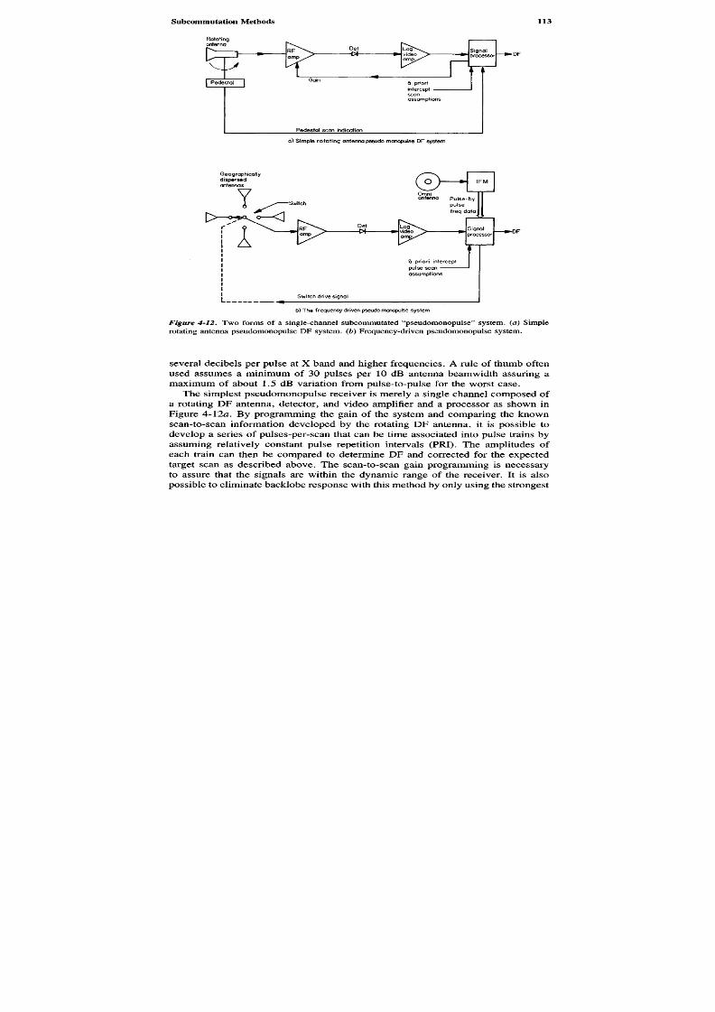
8/8/2019 SciTech - Microwave Passive Direction Finding
http://slidepdf.com/reader/full/scitech-microwave-passive-direction-finding 127/323
b) The frequency drven pseudo monopuse sysemFigure 4-12. Two forms of a single-channel subcommutated "pseudomonopulse" system,(a ) Simplerotating antenna pseudomonopulse DF system,(b) Frequency-driven pseudomonopulse system.
several decibels per pulse at X band and higher frequencies. A rule of thumb oftenused assumes a minimum of 30 pulses per 10 dB antenna beamwidth assuring amaximum of about 1.5 dB variation from pulse-to-pulse for the worst case.
The simplest pseudomonopulse receiver is merely a single channel composed ofa rotating DF antenna, detector, and video amplifier and a processor as shown inFigure A-YIa. By programming the gain of the system and comparing the knownscan-to-scan information developed by the rotating DF antenna, it is possible todevelop a series of pulses-per-scan that can be time associated into pulse trains byassuming relatively constant pulse repetition intervals (PRI). The amplitudes ofeach train can then be compared to determine DF and corrected for the expectedtarget scan as described above. The scan-to-scan gain programming is necessaryto assure that the signals are within the dynamic range of the receiver. It is alsopossible to eliminate backlobe response with this method by only using the strongest
Swtch drve sgna
a priori interceptpuse scanassumptons
Sgnalprocessor
IFMOmnantenna Pulse-by
pulsefreq data
Geographicalydispersedantennas
Swch
RFamp
DetDF
Rotatngantenna
RFamp
Pedestal
Det DF
Gain
SignalprocessorLog-videoamp
6 prioriinterceptscanassumptons
Pedesta scan indicationa) Smpe rotating anenna pseudo monopuse DF sysem

8/8/2019 SciTech - Microwave Passive Direction Finding
http://slidepdf.com/reader/full/scitech-microwave-passive-direction-finding 128/323
lobe of a scan that is know n to be unsaturated. This can be determined by exam iningscan-to-scan data with a computer. Although this system can and has been madeto work, it is not useful in dense environments since it takes excessive time.
A more practical type of subcommutated pseudomonopulse receiver substitutesmultiple antennas switched on a pulse-by-pulse basis as shown in Figure4-l2b andas described for radar receivers in Ref. 9. The input signal is received by anomniazimuthal antenna feeding an instantaneous frequency measurement (IFM)receiver that provides frequency data on each pulse . The signal processor associatesthe pulses into pulse trains by frequency and forms the DF ratio of the signalamplitude received on one antenna at timet\ with the same frequency signal receivedon the next adjacent antenna att2, where t2 - h is the derived pulse interval.Switching is done on a pulse-by-pulse basis. The pseudomonopulse ratio thusobtained is corrected by a priori knowledge of the intercept expected radar scan.The DF output of this system h as, in effect, been norm alized removing the interceptscan ratio to the extent of the accuracy implicit in the scan prediction.
4.3.2 True Monopulse Subcom mutated Receiver
Figure 4-13 is a diagram of a true monopulse frequency-driven subcommutated
receiver. An omnidirectional antenna feeds an IFM receiver that makes pulse-to-pulse measurements of the signal environment, feeding this information, groupedwith analog signal data, to a processor where digital frequency, pulse amplitude,time of arrival, and pulse-width data fields are formed. An eight-element antennaarray (shown here as two 45 degree offset-switched four element pairs of spirals)is switched as asequenced pairproviding two adjacent signals that develop a seriesof logarithmic ratio signals that are temporarily stored as DF angle-of-arrival possibilities(10). These analog logarithmic ratios are also provided to the processor for time-
of-arrival encoding. Once a set of pulses is frequency associated into a train bydata from the IFM subsec tion, it is possible, by time-of-arrival com parison , to makethe DF measurement, the frequency word acting as a filter to associate pulses intotrain using the time-of-arrival word to deinterleave the DF pairs from the environment.The DF is a true monopulse measurement, subcommutation being used as a meansto reduce the number of channels. High intercept probability is provided by om-niazimuthal IFM channel; however, DF measurement is slow, often requiring adecision as to whether or not to make it based on frequency and/or other omni-
measured characteristics.In the system shown above , low-gain w ideband antennas, such as planar spirals,
are paired to obtain the true monopulse ratio eliminating the correcting assumptionand requiring that each pulse be received inboth antennas of the pair. This reducesthe system sensitivity compared to the single-channel pseudomonopulse techniquedepending upon processing assumptions. Broadband RF switching is used, necessitatingthe use of matched switches. Two RF amplifiers are often added, to improvesensitivity of the D F channel m aking the switched-pair system sensitivity approximatelyequal to that of the omniazimuthal IFM receiver channel. In another configurationa number of narrow-beam octave horn antennas can be used to obtain higher sensitivity.
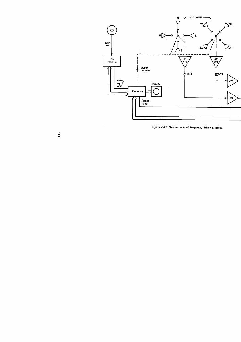
8/8/2019 SciTech - Microwave Passive Direction Finding
http://slidepdf.com/reader/full/scitech-microwave-passive-direction-finding 129/323
Figure 4-13. Subcommutated frequen
E T
RFamp
S
N
W
Switch
controller
Omniant
Analogsignalinput
IFMreceiver
Processor
Display
Analogratio

8/8/2019 SciTech - Microwave Passive Direction Finding
http://slidepdf.com/reader/full/scitech-microwave-passive-direction-finding 130/323
The improvement gained is due to the relative antenna gain of a horn compared toa spiral, permitting the video switching concept to be used at the expense ofinstantaneous frequency bandwidth, since the horns do not provide as wide an RFbandwidth. The sequenced offset-pair system shown is typical of a relatively complexsubcommutated system, the chief virtue of the paired technique being the trueamplitude monopulse DF normalization. It may also suffer from the physicallydifferent field of views of the omniazimuthal and DF antennas since they mustusually be placed at different locations. Some systems make use of a monopulsepair formed by the omni antenna and one switched antenna of a DF array. Theproblem with this approach , how ever, is the different gain and field-of-view betweenthe antennas due to construction, polarization, and physical displacement.
4 .4 SUPERCOMMUTATION
The problems in subcommutation can be overcome, in part, by the technique ofsampling or supercommutation. This is defined as the process of switching to eachof n antennas du ring the duration of a given pulsewidth for the purposes of obtainingthe monopulse ratio on a single pulse (11). This technique is most nearly equal to
monopulse in the formation of the ratios and has the incidental advantage of choppingCW and high-duty cycle signals by the high-speed switching action.Figure 4-14 is a diagrammatic representation of the technique. Four antennas,
having a finite RF bandwidth, are sampled by a high speed RF switch capable ofbeing activated at a rate that allows time m ultiplexing of each of their outputs w ithina single received pulse width. The resultant signal is amplified by a common RFamplifier, detected, and logarithmically amplified. Deinterleaving or separation ofthe original four signals is accomplished by a decommutator, synchronized with
Samplnggenerator
Ange ofarrival
DFcomputere-commutator
DLVA
Broadbanddetector
Figure 4-14. Supercommutated DF receiver.
RFamp

8/8/2019 SciTech - Microwave Passive Direction Finding
http://slidepdf.com/reader/full/scitech-microwave-passive-direction-finding 131/323
the RF switch, permitting recovery of the four original video signals, which arethen formed into the appropriate amplitude monopulse ratio of strongest to nextadjacent strongest signal. The ratio thus formed is the familiar amplitude monopulsedata, which can then be processed as before.
Ordinarily, supercommutation must be done at a rate consistent with the Nyquistcriteria, which states that if the occupancy of the pulse signal band is limited toB1, the rate must be2B1. This would typically require a 20 MHz rate for a 10 MHzwide occupancy pulse signal. The need to interleave four signals, however, necessitatesthe use of a rate consistent with the rise and fall times of the interleaving switching,which is at least four times faster (for a four-antenna system). Typical bandwidthsof 80-200 MHz are therefore used for video and logarithmic amplifiers in systemsof this type.
Supercommutation, as a technique, allows multiplexing of RF signals by timedivision. The isolation between any two adjacent channels determines the maximumdifference of RF amplitude that can be accommodated. If, for example, 25 dB ofisolation is obtained, then the range of signal in one beam of an antenna to thatof the next adjacent one could use this value, allowing a high articulation or rateof pattern change-per-degree of arrival angle, which is desirable for maximumaccuracy. The limiting factor in obtaining high isolation is the time it takes to go
from one arm of the switch to the next. The limit to the number of channels to besupercommutated becomes the dwell time and change-of-state time for the switching.For this reason, practical systems have been confined to four or five channels. Withthe development of faster switches, the technique could be expanded to multihornarrays for example. The combination of the multiple input channels, incidently,eliminates the problem of RF combining that would occur if adjacent antennas wereRF summed.
In the supercommutated system, as shown in Figure 4-14, the four video signals
are recovered completely before the processing subsystem is used to determinepulse parameters, time of arrival, and monopulse direction. This requires that ananalog-to-digital conversion take place late in the system to permit digital processingfor signal recogn ition. In the generic warning receiver, a signal processing computerwould form a digital word or field for each signal. For example, a typical interceptmight have an 8-bit word for angle of arrival and signal amplitude, a 16-bit wordfor arrival time, another8-bit word for antenna beam and pulse probability char-acteristics, and, in some receivers, a 16-bit word for frequency. These conversions
would be made and the resultant digital words loaded into storage for processing,usually dynamic random access memory (DRAM) is used for this purpose, makingthe storage a time-consuming process.
Supercommutation develops much information in a form that can be processedrapidly by virtue of comparisons that can be made in near real time. Figure 4-15shows an adaptive supercommutated DF system that performs signal preprocessingin advance of loading of the memory of the computer for the purposes of savinganalog-to-digital conversion and storage loading time. In the hypothetical systemshown, all data developed by the supercommutation process is reconstituted into"parallel compare" channels and fed to a preprocessor comparator where DF, signal
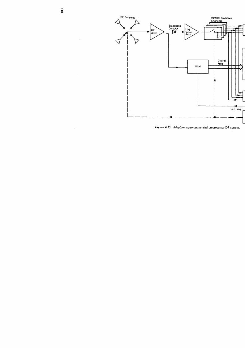
8/8/2019 SciTech - Microwave Passive Direction Finding
http://slidepdf.com/reader/full/scitech-microwave-passive-direction-finding 132/323
Figure 4-15. Adaptive supercomm
BroadbandDetector
D FAntennas
RFA m p l
LogVideo
A m p

8/8/2019 SciTech - Microwave Passive Direction Finding
http://slidepdf.com/reader/full/scitech-microwave-passive-direction-finding 133/323
amplitude, and other information can be extracted during the duration of the incomingpulse. This can be done by structuring the architecture of the preprocessor specificallyfor this purpose. Since it is possible to make comparisons faster with high-speedgates than it is to perform an analog-to-digital conversion, load a random accessmemory, and then do the processing; time is saved. If DF driven, monopulse DFdecisions can be used to stop the supercommutation switch at the antenna receivinga desired signal, feed the RF from this antenna to the instantaneous frequencyreceiver (IFM), and then develop a digital frequency word. Since IFM frequencymeasurement is usually the slowest part of the process, only pulses that meet thedirection-of-interest criteria will be measured, reducing the shadow time of thereceiver substantially. The decision-making process in this system, however, isbeing performed on a single or monopulse requiring very large signal-to-noise ratiosto reduce false alarms. This requirement is fortunately in concert with the abilityto make the crystal receiver highly sensitive or noise-limited by use of a singlelinear RF amplifier. The single-channel time multiplexing eliminates channel-to-channel balanc ing that would be required in a multichannel parallel system; how ever,the switch balance, isolation characteristics, and dynamic range capabilities mustbe carefully controlled.
The preprocessor supercommutated system is a compromise between sensitivity
and total intercept probability since it sacrifices the higher sensitivities of the narrowervideo bandwidth amplified crystal video receiver for the feature of direct comparisons(true monopulse) and the ability to measure frequency selectively. It exhibits onlymoderate operating sensitivity, in the order of that of a standard radar warningreceiver. The availability of the frequency word to act as a sorting tool, however,is a desirable feature. The system is also limited by finite switching capabilities,placing a limitation on the minimum pulse width that can be used. As a practicalmatter, the adaptive supercommutated preselector receiver is a good example of
the trade-offs that can be made between relatively low-cost digital componentryand expensive RF circuitry.The advantages of supercommutation, which is actually time-division multiplexing
(TDM), is the relative simplicity and balance improvement obtained by the use ofa single amplification and detection channel for all four directional signals. Theoccupancy bandwidth of the switching processes, however, makes the system subjectto problems of noise, which must be considered in any system design trade-offsince the commutation process generates noise and harmonics at the rise-time rate
of switching, which could generate harmonics that can appear in the RF passbandof the receiver. The supercommutation technique does yield data on a single pulsebasis, therefore placing it in the category of a true monopulse system.
4.5 MONOCH ANNEL MONOPULSE
One of the major problems in developing monopulse receivers capable of coveringan instantaneous 360 degree field-of-view is the need to replicate as many receivechannels as there are antennas to form the monopulse ratio of strongest to next

8/8/2019 SciTech - Microwave Passive Direction Finding
http://slidepdf.com/reader/full/scitech-microwave-passive-direction-finding 134/323
strongest signal. The problem is made more acute than that of channel cost by theneed to match the amplitude and, in some cases, phase of the channels over a widedynamic rang e. In the approaches presented to date, we have studied both subcom-mutation or pseudomonopulse and supercommutation or time-shared multiplexingas usable techniques; there is an analogous phase equivalent to supercommutationthat merits our attention. This novel form of monopulse detection, developed byWatkins Johnson (12), utilizes a single shared channel and makes use of many ofthe principles of the time-multiplexed supercommutator without the disadvantagesof expensive commutation and decommutation. It accomplishes this by phase-tagging each of the four (or more) amplitude DF signals such that a single super-heterodyne channel can process the resulting composite signal, thus eliminatingbalance problems as before.
To do this requires that each of the four signals to be dow nconverted be uniquelyidentified during the duration of the pulse width. In a supercommutated system thisis done by the time position of a signal; that is, the RF switch that samples eachchannel is time synchronized with the video distribution switch to charge a capacitorto deinterleave that channel thus recovering the DF data. In the monochanneltechnique the phase state of the local oscillators that downconvert each of thechannels differs from each other in a known way to identify or tag that channel.
Knowledge of this coding is then used in the IF-to-video conversion to separatethe signals in the demodulation process to recover the original channels.Figure 4-16 is a simplified diagram of the technique. Each channel of a four-
spiral antenna system is downconverted to a convenient IF by a double-balancedmixer fed by a local oscillator signal from each one of four biphase modulatorsAfi, M2, M3, and M4. The biphase modulator introduces a pass (1) or no pass (0)state to the local oscillator signal essentially creating a phase-code modulated signal.The code is a maximum linear sequence that makes each local oscillator signal
appear as a pseudorandom signal with an occupancy of the form of sinxlx. Thecode generator generates this sequence, which is then delayed or time-shifted bythe delays t\, t2, and r3, these delays providing the signal isolation necessary to tageach of the RF signals. The single channel, which now contains the four channelsof DF data, is amplified and brought down to a convenient IF where the coded RFsignal is then used to decode the phase state of the phase-modulated compositesignal back into the four original DF signals, each of which can then be processedto extract DF data.
The above method is a true monopulse technique to the extent time supercom-mutation is, since the code rate must be selected to allow four states of phase tobe obtained within a pulse width. Typical code rates are 200 MHz for a 200nanosecond pulsewidth. At this value, there is approximately 15-18 dB isolationbetween channels, which is sufficient to permit the use of spiral antennas sinceapproximately 12 dB of signal difference occurs between two spirals at boresightwhen adjacent channels are compared (see Chapter 9, squint accuracy discussion).The monochannel technique can also include a fifth channel, an omniazimuthal foruse with an IFM, for example. This would require readjustment of the rates.

8/8/2019 SciTech - Microwave Passive Direction Finding
http://slidepdf.com/reader/full/scitech-microwave-passive-direction-finding 135/323
Figure 4-16. Monochannel phase encoding mon
Spiralants
L o c a losc i l l a to r
Tuningdata
C o d egenerator

8/8/2019 SciTech - Microwave Passive Direction Finding
http://slidepdf.com/reader/full/scitech-microwave-passive-direction-finding 136/323
The significant advantage, outside of the obvious cost saving of the monochannelapproach, is that it again permits combination of the four RF signals into a singlechannel w ithout the problem s of interferometer nulling or the generation of "gratinglobes," which would occur if direct RF addition were attempted. The technique ismost suited to relatively narrow bandwidth scanning superheterodyne receiverscompared to supercomm utation, which is best applied to wide RF bandwidth no ise-limited crystal video receivers.
4.6 PARALLEL DF CHANNEL IZATION
Parallel DF channelization DF receivers make use of array techniques or multipleantennas to provide wide-angle DF coverage. We will be covering arrays as aseparate topic in Chapter 5; how ever, for the purposes of illustration of the techniqueconsider Figure 4-17, showing the parallel arraying of individual antennas utilizingbacklobe inhibition. The system shown is well suited for applications requiring
Horn antenna
DLVALim
DFcomputer
(Same)
Frequencyreceiver
Pulseprocessor
Computer
Activitydisplay
F
re
q
Angle
RFamp
Halfomniant
Figure 4-17. Parallel DF channelization receiver.

8/8/2019 SciTech - Microwave Passive Direction Finding
http://slidepdf.com/reader/full/scitech-microwave-passive-direction-finding 137/323
dispersed antennas, although single-point arrays are also in use. Each channel inthe configuration shown makes use of a high-gain antenna limiter, detector, andvideo amplifier channel to provide coverage of a specific angular sector. Logarithmicamplifiers are used in each channel to permit direct comparison of all channels.Two half-omnidirectional antennas each covering approximately 180 degrees ofview are used to provide backlobe inhibition of the horn array. These antennasconveniently provide an RF output to feed an instantaneous frequency receiver(p . 78).
The parallel DF channelized receiver offers many advantages, the chief beingfull omniazimuthal coverage at all times. The system can be either DF or frequencydriven and can be readily coupled to an equivalent jamming system for both retro-directive and repeater jamming. The system also offers an immunity to jammingor overloading by strong CW emitters, since at the worst, only one or two sectorsmight be disabled. The parallel channelization concept is a powerful approach tojamm ing immunity. Although simple horn antennas are shown here, array techniquesutilizing Butler matrixes, Rotman-Turner lens feeds, and ferrite phase shifting arein wide use and will be described in the next chapter. Since systems of this typeare generally large, the output display is expanded to provide ELINT as well asthreat information, giving this type of output an activity view of the electromagneticenvironment around the host vehicle.
4.7 MULTIBEAM DF ARRAYS
Parallel multibeam array DF systems make use of an antenna system that providesa contiguous pattern coverage either for a sector or over a full 360 degrees. Thesetypes of systems are readily made conformal to the host vehicle as shown in Figure
4-18, which is one 90 degree sector of a 360 degree coverage system. In actuality,in a shipboard installation, two DF units would be used to cover 180 degrees onthe port side and two more to cover 180 degrees of azimuth on the starboard side.In the system shown, the 16-beam multibeam array identifies the angle of arrivalin just one 90 degree sector. The half-omniazimuthal antenna, which is similarlypolarized and placed in close proximity to the DF array(s), feeds an IFM receiverto obtain frequency data. A digital tracking unit develops monopulse DF information,time-of-arrival, and frequency, all of which are grouped into threat words and fed
to a computer for threat identification. This information is displayed to an operatorwho can take appropriate countermeasures, ranging from dispensing of chaff in theappropriate direction to application of ECM for larger systems. In this latter case,a series of travelling wave tube (TWT) amplifiers can be supplied theangle-of-arrival data directly and their outputs combined in a lens array to transmit a signalin the same direction as that of the input pulse. The two 90 degree sector 16-beamantenna systems combined with fore and aft beamformer antennas can be directlyswitched to a 35-multibeam array network fed by as many TWTs as there are beam
ports. A modulated signal return would then be generated, amplified, and directedto retrodirectively jam the target, using appropriate modulation modes. The power
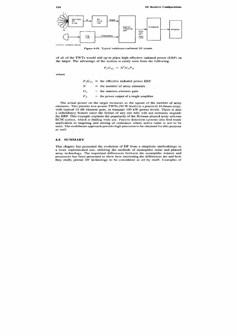
8/8/2019 SciTech - Microwave Passive Direction Finding
http://slidepdf.com/reader/full/scitech-microwave-passive-direction-finding 138/323
of all of the TWTs would add up to place high effective radiated power (ERP) onthe target. The advantage of the system is easily seen from the following:
PjGAj = N2G6P A
where
PjGAj = th e effective radiated powerE R P
Af = the number of array elements
Ge = the antenna element gain
PA = thepower output of a single amplifier
The actual power on the target increases as the square of the number of arrayelements. This permits low-power TWTs(50 W level) in a practical 16-beam array,with typical 10 dB element gain, to transmit 100 k W power levels. There is alsoa redundancy feature sinceth e failure of any on e tube will n o t seriously degradethe ERP. This example explainsth e popularity of the Rotman phased array antennaECM system, which is finding wide u s e . Passive detection systems also find readyapplication to targeting a n d aiming of ordinance where active radaris no t to beused. T h emultib eam app roach permits high precisionto be obtained for this purpose
as well.
4 . 8 S U M M A RY
This chapter h a s presented th e evolution of D F from a simplistic methodology toa more sophisticated o n e , utilizing the methods of monopulse radar an d phasedarray technology. T h e important differences between th e monopulse sensors an d
processors h as been presented to show h o w interesting th e differences are and h owthey really permit D F technology to be considered as art by itself. Examples of
Figure 4-18. Typical multibeam conformal DF system.
1/2 Omn azimuthal channel
FMrcvr
Frequency
Digitaltrackingunit Data
freqDFpulsedata
ComputerDisplay
AngleFrcvrs(16)
160° FOVantarray
16

8/8/2019 SciTech - Microwave Passive Direction Finding
http://slidepdf.com/reader/full/scitech-microwave-passive-direction-finding 139/323
key systems have been used to present the more useful approaches, within theconfines of previously released information. This practice will be followed through-out this book to familiarize the reader with the various forms of DF technology. Itwill become apparent that despite the many different paths passive microwavedirection finding has taken over the years, actual systems really converge intofundamental types: rotary DF, commutated systems, interferometers, and parallelfixed antenna arrays.
R E F E R E N C E S
1. BeIk, J., J. Rh odes, and M. Thornton, "Radar Warning Receiver Subsystem s,"Microwave Journal,Sept. 1984, p. 199.
2. "Egypt Deploys British ESM," Staff Report,Electronic Warfare,Defense Electronics, Vol. 10,No. 1, p. 79, Jan. 1978.
3. LaTourrette, P., "Multiplexers for ESM Receivers," Conference Proceedings, Military Microwaves,the Institution of Electrical Engineers and Institution of Electronic and Radio Eng ineers, O ct. 1978,pp. 9 ff.
4. "U.S. Steps Up Its Power Management Program," Staff Report,Electronic Warfare,Vol. 6, No.3, May/June 1974.
5. "Digital Threat Warning System Completes Tests, Nears Army Contract,"Aviation Week and SpaceTechnology,May 6, 1985.
6. "The AN/ALR -80 RWR S ystem ," Data Sheet, General Instrument, Government Systems Division,Hicksville, NY .
7. Bullock, L ., G. Oe h, and J. Sparagna, "An Analysis of W ide-Band Microwave Monopulse DirectionFinding Techniques,"IEEE Transactions on Aerospace and Electronic Systems,Vol. AES-7, No.1, Jan. 1971, p. 189.
8. Page, R. M., "Accurate Angle Tracking by Radar," NRL Report RA3A222A, Plate 1, Dec. 28,1944. Republished inRadars Vol. I, Monopulse Radar,Dedham, MA: Artech House, 1977.
9. Stone, T. W., "IF Comm utation Increases Monopulse Radar Accuracy,"Microwave Systems News& Communications Technology,Dec. 1985.
10. Lipsky, S. E., "Method and Apparatus for Electrically Scanning an Antenna Array in a MonopulseDF Radar System," U.S. Patent 4,313,117 granted Jan. 1982.
11. Lipsky, S. E., "Supercomponents Solve New DF Design Problems,"Microwaves,Sept. 1975.
12. Klaus, D., and R. Hollis, "Monochannel Direction Finding Improves Monopulse Techniques,"Defense Electronics,Vol. 14, No. 3, Mar. 1982.
8/8/2019 SciTech - Microwave Passive Direction Finding
http://slidepdf.com/reader/full/scitech-microwave-passive-direction-finding 140/323
DF Antenna Arrays
Array technology for passive direction finding has been developing as an outgrowthof two factors: first, the need to respond retrodirectively (transmit in the samedirection as received) to a threat for jamming purposes; second, the need to measurea signal to a high degree of accuracy for targeting or aiming purposes. One of themain concepts of the field of electronic support measures (ESM) is the use of theelectronic receiving systems as a means to detect signals for threat determinationoptimally and as a method of improving or multiplying the effectivity of jammingor electronic countermeasures (ECM). These functions are a subset of the conceptof electronic warfare. With the advent of phased arrays, passive direction finding
has again stolen a page out of the handbook of radar design.Early radar systems first utilized scan then monopulse passive lobing in thereceiver to illuminate and detect targets. As the number of targets (and radars) ina given environment increased, it became obvious that improved resolution in allareas would be needed. Doppler, moving-target indicators, and range-gating techniqueswere honed to a high degree of perfection to improve range resolution, and monopulseimprovements normalized the radar signal returns, reducing false clutter and glintvariations. Despite these changes, it became obvious in the early 1950s that fundamental
changes would be needed in the antenna systems to improve angular resolution inboth azimuth and elevation. Additionally, the requirement for improved securityfor countermeasures immunity and the ability to be able to adapt to changingconditions of the environment acted to advance the concept of a narrow beamwidthrapidly "steered" antenna. Arraying or essentially combining the effects of manyelemental radiators to form one or more beams developed as a technique that couldaccurately direct or position a beam in free space, the arraying and combinationaleffects permitting development of antennas that could generate narrow beamwidths
with high gain that could be switched or scanned. Since the maximum range of aradar is directly proportional to the effective radiated power (ERP), which in turn
Chapter Five

8/8/2019 SciTech - Microwave Passive Direction Finding
http://slidepdf.com/reader/full/scitech-microwave-passive-direction-finding 141/323
depends upon relative gain over an isotropic radiator, narrowing of the antennabeam widths acted to improve range over the limits imposed by available transm ittersand receivers.
A corollary advantage to the gain, obtained at the expense of reduced beam widthsin radar transmitters, was the distributed pow er concept inherent in any multielementradiating system. Simply stated, since there are many radiators, it is possible toconnect each one to a separate source of RF power each of which, if made phasecoherent, can effectively add its pow er in space, in contrast to the problem ofgenerating a single source of high power and connecting it to a steered antennasystem. The advantages of this distributed source technique become more importantwith solid-state oscillators. High power solid-state transmitters are still unavailableat high microwave frequencies, yet moderate power levels are obtainable fromsolid-state oscillators and amplifiers, which when properly phased and added, cancreate the desired high ERP necessary to achieve the required range improve-ments.
There are many phased array techniques in use at the present time that are oflittle interest in passive direction finding since they are highly dependent upon apriori knowledge of the transmitted signal. We will confine our consideration totypes that require no such data. Phase arrays permit the accurate angular reception
of signals by means of a high-gain narrow-angle beam scanned over the field ofview (FOV) the array is designed to cover. A simple case is the planar array ofmultiple elements spaced in a straight line and fed in a phase , amplitude progression,or time sequence to effectively switch or scan over azimuth (((>) and elevation (0)in a prescribed manner. By planar, it is understood that all radiating elements liein one plane and that desired operation occurs only over a limited angle, typically± 60 degrees from the perpendicular boresight or pointing angle of the plane ofthe array. If greater angular or hemispherical coverage is desired, a multidimensional
array can be constructed by mounting assemblies of planar arrays about a hostvehicle conformally or by constructing a four-faced pyramidal structure with anarray mounted in each planar face. Each approach has its features: A conformalarray encloses the host vehicle minimizing its shadowing or interfering effects; astand-alone array minimizes problems of phase coherence and equalization of powerfeeds and centralizes the system for repair and maintenance. Another approach tohemispherical coverage is to eliminate the planar concept and mount the radiatingelements cylindrically on the surface of a circular surface of sufficient diameter to
permit appropriate phase and amplitude correction to be made to compensate forthe nonplanar configuration.
In passive direction finding, use is often made of another implementation of thephased array, known as the adaptive array. Since it is desirable to receive a signalwith the best signal-to-noise ratio, any information or decision that can steer orpoint the array beam in the optimum direction in anticipation of the signal will beof great help. The ability to reject undesired signals at different angular positions,with respect to the array, is also advantageous. The capability of programming anarray offers potent features for future systems as computer decision making takesover the operation of DF systems.
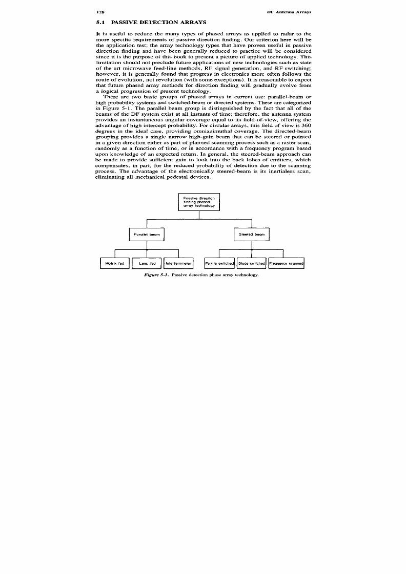
8/8/2019 SciTech - Microwave Passive Direction Finding
http://slidepdf.com/reader/full/scitech-microwave-passive-direction-finding 142/323
5.1 PASSIVE DE TEC TIO N ARRAYS
It is useful to reduce the many types of phased arrays as applied to radar to themore specific requirements of passive direction finding. Our criterion here will bethe application test; the array technology types that have proven useful in passivedirection finding and have been generally reduced to practice will be consideredsince it is the purpose of this book to present a picture of applied technology. Thislimitation should not preclude future applications of new technologies such as stateof the art microwave feed-line methods, RF signal generation, and RF switching;however, it is generally found that progress in electronics more often follows theroute of evolution, not revolution (with some exceptions). It is reasonable to expectthat future phased array methods for direction finding will gradually evolve froma logical progression of present technology.
There are two basic groups of phased arrays in current use: parallel-beam orhigh probability systems and switched-beam or directed systems. These are categorizedin Figure 5-1. The parallel beam group is distinguished by the fact that all of thebeams of the DF system exist at all instants of time; therefore, the antenna systemprovides an instantaneous angular coverage equal to its field-of-view, offering theadvantage of high intercept probability. For circular arrays, this field of view is 360degrees in the ideal case, providing omniazimuthal coverage. The directed-beamgrouping provides a single narrow high-gain beam that can be steered or pointedin a given direction either as part of planned scanning process such as a raster scan,randomly as a function of time, or in accordance with a frequency program basedupon knowledge of an expected return. In general, the steered-beam approach canbe made to provide sufficient gain to look into the back lobes of emitters, whichcompensates, in part, for the reduced probability of detection due to the scanningprocess. The advantage of the electronically steered-beam is its inertialess scan,
eliminating all mechanical pedestal devices.
Passive directionfinding phasedarray technology
Parallel beam Steered beam
Matrix fed Lens fed Interferometer Ferrite switched Diode switched Frequency scanned
Figure 5 - / . Passive detection phase array technology.

8/8/2019 SciTech - Microwave Passive Direction Finding
http://slidepdf.com/reader/full/scitech-microwave-passive-direction-finding 143/323
Any antenna can be considered to consist of a set of identical radiating elements,such as dipoles or slots, configured in a pattern such that under all conditions eachelement operates as each other. This includes the effect of mutual coupling betweenthe elements and the effects common to all. For this given set there is an elementpattern that is multipled by another pattern termed the array pattern (1) of the form:
N Cg(u) = 2 cxp(jkxnu) ie(y) exp(jkyu)dy (5-1)
= f(u)e(u) (5-2)
where
ie = the current density across the array
x = the location of the element(xn)
y = x - nn
dy = dx
The two functions in Equation (5-2) are each radiation patterns; the first,/(w),being the array factor, the second,e(u), the element factor. This latter term isconcerned with the excitation of each radiating element, which should be the same.The array factor is of prime importance since it establishes the pattern based uponthe physical geometry of the radiating antenna structure. An array can be steeredor scanned by series-feeding each element through an amplitude-weighted phaseshift. This may be done in time by switching or by frequency scanning. To obtainfixed beamwidths that are always present, the elements of the array may be fed in
parallel all of the time through a feed network that presents the appropriate phasedifferences to each radiating element. The steered-beam antenna can be made toexhibit array gain; the parallel beam antenna generally does not. We shall discussthe parallel array in this chapter as an array and in Chapter 6 as an interferometer.The frequency-scanned array, while of great importance in radar, finds little use inpassive direction finding systems, since it does not generally exhibit the primarycharacteristic, wide instantaneous RF bandwidth, needed for high intercept probability.
5.2 PARALLEL BEAM FORM ED ARRAYS
Since this type of antenna provides maximum coverage, it has become of greatimportance in passive ELINT and warning systems, where the complexity and sizeof the array and its associated circuitry can be tolerated. Most applications arefound in naval systems. The planar array function can be obtained directly by aseries of n parallel horn antennas as described in Chapter 4. In this case, the arrayis composed of the set of horn rad iators, each of which exhibits gain in the directionof arrival perpendicular to the mounting plane. Amplitude comparison of the log-

8/8/2019 SciTech - Microwave Passive Direction Finding
http://slidepdf.com/reader/full/scitech-microwave-passive-direction-finding 144/323
detected n channels will give the monopulse ratio to a high degree of accuracy andwith a sensitivity determined by the horn gain over an isotropic antenna. The ratiocan also be found by comparison to an omniazimuthal (360 degree field-of-view)or half-omniazimuthal (180 degree field-of-view) antenna for moderate accuracyand backlobe suppression as shown in Figure 4-17.
The advantage of this type of system is the ability to use conformal mount orgeographical displacement of the antennas around a ship or plane. The disadvantageis the limited RF band widths of the horn s. T his is due to the fact that the gain ofa horn antenna varies directly with the square of the frequency. The gain is usuallychosen for a minimum gain at the low-frequency end, which results in high gainand an associated reduction of antenna beamwidth at the high-frequency end. Thechange in pattern shape, as a result, requires that frequency information be availableto correct the DF look-up tables. An array of horns also suffers from spacingproblems since high efficiency cannot be obtained with good beam crossovers unlessthe horns are closely spaced. It has also been determined that each horn shouldexhibit a sin x/x antenna pattern for maximum efficiency. This would lead to theconclusion that a uniform amplitude illumination be present, which is not practical.For these reasons, parallel horn systems become difficult to use although, simplistically,the ease with which paralleled amplitude detected channels can be compared is
attractive. Double-ridged horns and frequency variable aperture area approacheshave been used to extend horn bandwidths, but in general, paralleled horn feedsare confined to an octave, making any broadband (2-18 GHz) system relativelycomplex.
5.3 PLANAR BUTLER ARRAY
The matrix or hybrid network generally of the form developed by Butler (2) isanother solution to arraying often used in planar array s. This feed ne twork typicallytakes the form of Figure 5-2, which is ann input, TV output connection of a seriesof quadrature couplers, 180 degree hybrid combiners, and phase shifters interconnectedto provide a progressive phase shift to each element of the planar array. Theprogressive phase shift concept derives from early work by Blass (9) and others.Essentially, a multiplicity of radiating elements will transmit a beam broadside totheir plane if they are all in phase. If the phase between the elements changesprogressively by 2itd/\, where d is the spacing between the elements, then theresulting pattern will point in the direction of the length of the line connecting allelements (endfire). It is then obvious that varying the phase progression betweenthe two extremes can steer the resultant antenna beam.
The above case considers a feed network with one input and a multiplicity ofoutputs, each of which feeds a radiating element in some form of phase progression.If a parallel network ofn inputs and TV outputs is used, it is possible to generateparallel rather than scanned or sequential beams. Since these beams are generatedby elements fed not in phase with one another, they can overlap without the undesirablecoupling effects of the simple parallel horns described above, eliminating intercouplinglosses and allowing attainment of an elemental sinxlx radiation pattern. Figure

8/8/2019 SciTech - Microwave Passive Direction Finding
http://slidepdf.com/reader/full/scitech-microwave-passive-direction-finding 145/323
Figure 5-2. Eight-port Butler matrix using 90 degree hybrid couplers and phase shifters.
5-3 shows the beams developed by the network shown. Each beam is lettered left(L) or right (R) of boresight and is available at the bottom of the feed matrix fordetection and comparison to an omniazimuthal antenna or the sum (from a detector)of all of the beams to form an amplitude monopulse ratio. It is also possible tomeasure the phase difference; however, the multiplicity of channels does not favorthis approach. Reference (3) gives design equations and discusses three beam in-terconnections of the eight-element antenna. In the system described here, beam
ArrayElements(n = 8)
ButlerMatrixOutputPorts(n«8)
FixedPhaseShifters
4-Port HybridCouplers
ButlerMatrixInputPorts(n=8)
IRLRLRLRL
Figure 5-3. Simultaneous eight-beam radiation pattern from an antenna array fed by an eight-port B utlermatrix.

8/8/2019 SciTech - Microwave Passive Direction Finding
http://slidepdf.com/reader/full/scitech-microwave-passive-direction-finding 146/323
crossover occurs at —4 dB , with adjacent beam isolation of about 20 dB . Antennabandwidth is approximately one octave. The position of the beam peaks varies asa result of the presence of X in the equations (Ref. 3 p . 263), requiring the use offrequency correction to assure that all dispersive phase shifts can be compensatedfor.
5.4 CIRCULAR BUTL ER-FED ARRAY
The planar Butler-fed array is somewhat limited by the above considerations; however,it is also possible to utilize the Butler matrix feed to excite a circular array ofradiating elements. If the elements are designed properly, it is possible to obtain a3:1 or greater RF bandwidth. The circular array was first described in the early1960s. In most applications, development of a series or sequential-switched beamwas desired, and most concepts followed the reasoning of the planar array in thisregard. It was realized that in a circular array the contribution of each element wasnot identical to the planar array since in the latter, each element is separately excitedand can be easily expressed as such for each term in the general equation of thearray factor.
In the circular array, the excitation can be considered to be a current distribution(4) I(x) of many individual currentsIn exp(y>u), where n ranges between —Nand+Af. The radiation pattern is
n=N-\
E(W) = E Ane>n* (5-3)
N=O
where
N = the number of elementsAn = a set of complex constants of currentIn multiplied by a Bessel function
Jn(X)
When Equation 5-3 is compared for a linear array ofN (elements),
n=N-lE m = 2 Ke? n * (5-4)
where
2s(<|>) = array factor
A(n) = the nth amplitude excitation coefficientsK = d/X

8/8/2019 SciTech - Microwave Passive Direction Finding
http://slidepdf.com/reader/full/scitech-microwave-passive-direction-finding 147/323
fx = 2T:K COS (f)
d = element spacing
It may be seen that the circular array is similar to the linear array, differing mainlyby the use of elemental current excitation in place of the amplitude or elementexcitation coefficients.
From this it follows that a circular array can be excited in a similar way comparedto the linear array. Shelton (5) and Chadwick and Glass (6) describe networks tofeed circular arrays in detail; however, it can be shown that the Butler matrix feed,described above, will provide parallel output patterns that are relatively insensitiveto elevation 0, varying as the sin 6, and that the current excitation varies linearlyacross the elements with a phase difference of(2TtK)ZN. There will be TV currentmodes corresponding toK = 0 ± 1, . . .(N- 2)/2, Nil. The total phase variationaround the array is 2i:K for the kth mode. By comparing the nonadjacent or plusand minus modes, for example,K= +2 to n = —2, an output phase variation ofmf), in this case four times the arrival angle, will result. The Butler-fed array istherefore capable of high resolution (articulation), which we continually note to bethe characteristic of phase monopulse systems that permit attainment of high-precisionDF measurements with this technique.
The condition for high accuracy for a Butler-fed circular array dictates the useof more elements than output ports to increase phase resolution, which in turnnecessitates that unused output ports be terminated. The Bessel termAn in Equation(5-3) must be nonzero, requiring that the radius of the circular array be chosen toprevent cancellation of the radiator element contributions or that directional rad iatorsbe used to prevent mutual coupling effects. When the output ports of the Butlerfeed network are paired, narrow beams will not be obtained at each output port as
was the case for the planar array(n = N). Sets of phase differences are obtainedbetween the pairs of ports that contain the angle of arrival, which, depending uponthe pairing, is some multiple of the actual phase difference between radiatingelements.
An excellent example of a Butler-fed circular array covering 2 -1 8 GHz is a DFsystem designed by Anaren Microwave Inc., shown in Figure 5-4, a diagrammaticblock diagram of the concept. The radiating structure consists of 32 horizontallypolarized slot antennas each fed by a coaxial cable connected across the slot at its
narrowest point. The slot tapers outward containing the horizontalE field, until thefield radiates from each element as a horizontally polarized signal at the outerdiameter. This is shown in Figure 5-5, a photograph of the printed circuit antennaelement array mounted atop a foam spacer and the lower biconical reflector. Thetips of the slots meet at the widest poin t, giving the appearance of a series of m etallicpetals; however, the slots , not the petals, radiate in the horizontal polarized direction.The antenna printed circuit card is mounted between two biconical reflectors pur-posefully to constrict the elevation angle (6) to + 4 0 - 1 0 degrees from a zero degree
horizon reference. The circular cutout behind each feed point is a high impedancematching transformer.

8/8/2019 SciTech - Microwave Passive Direction Finding
http://slidepdf.com/reader/full/scitech-microwave-passive-direction-finding 148/323
Figure 5-4. A 32-element Butler-fed circular array. Courtesy of Anaren Microwave Corp.
Each of the 32 coaxial cables is fed to an input port of a Butler matrix consistingof a series of hybrids, quadrature couplers, fixed phase shifters, and power dividersas indicated. This configuration is diagrammed in Figure 5-6, where it can be seenthat the output ports are paired to providen = 0, n = ±1, n = ±2, and n = ± 4beams. Only the referencen = 0 is compared to /z X 1,n X 2, and n X 8. Thistechnique gives a phase variation of c(), 2c|>, and 8c() for a physical input angle ((),thereby increasing the resolution of the system. The ambiguity of the high resolutionn x 8 port is compared to then = 0 port giving high-phase sensitivity but with
four ambiguities. These are resolved by phase comparison of then x 2 pair with
Fixed Phase Shifters80° Hybrds
Power Dividersuad Hybrids
32 ElementCircular Array

8/8/2019 SciTech - Microwave Passive Direction Finding
http://slidepdf.com/reader/full/scitech-microwave-passive-direction-finding 149/323
the n = O, which has two ambiguities that are finally resolved by then x 1 phasecomparison to n = 0, which has no ambiguities. Since each phase angle is binaryrelated, it is convenient to use this technique to develop an8-bit digital word. Phasecomparisons are made by broadband phase discriminators or correlators, anotherform of the class III monopulse system described in Chapter 2, Section 2.3. Thecorrelator is described in detail in Chapter 10, Section 10.2.
Omniazimuthal output for an IFM or pulse detection channel can be obtainedby amplitude detection of then = 0 channel since this represents the energy summedfrom all elements of the array, and the system, in fact, makes use of this channelfor that purpose.
The system shown has undergone extensive testing and is capable of providing
2 degree RMS accuracy over a wide range of operating characteristics. Figure 5-7is a photograph of the 7.5-18.0 GHz array sited above the 2.0-7.5 GHz array,the latter covered by a polarizer that converts the received slant linearly polarizedsignal to horizontal polarization at the antenna element slots. The receiver attainsa - 6 0 dBm sensitivity in the low and - 5 5 dBm in the high band. The overalloperating accuracy when mounted in the radome (shown beside the antenna structure)and measured on a ship is between 1.78 and 2.6 degrees RMS, which are excellentresults. This compares with a 1.5 degree RMS typical accuracy as reported by
Anaren in anechoic chamber tests.
Figure 5-5. Anaren radiating structure. Courtesy of Anaren Microwave Corp.

8/8/2019 SciTech - Microwave Passive Direction Finding
http://slidepdf.com/reader/full/scitech-microwave-passive-direction-finding 150/323
Figure 5-6. Configuration of a 32-element DF measurement system. Courtesy of Anaren MicrowaveCorp.
Ambiguity
ResolvingNetwork
8 BitAngle of Arrival
DigitalPhase
Comparator
DigitalPhase
ComparatorDigitalPhase
Comparator
DigitalPhase
Comparator
Solid State RFAmplification
AntennaFeedNetwork
32 Element Circular Array360 Degree Coverage
Ref842l

8/8/2019 SciTech - Microwave Passive Direction Finding
http://slidepdf.com/reader/full/scitech-microwave-passive-direction-finding 151/323
Figure 5-7. The 2-18 GHz Anaren circular array antenna system shown with polarizer and radome.Courtesy of Anaren Microwave Corp.
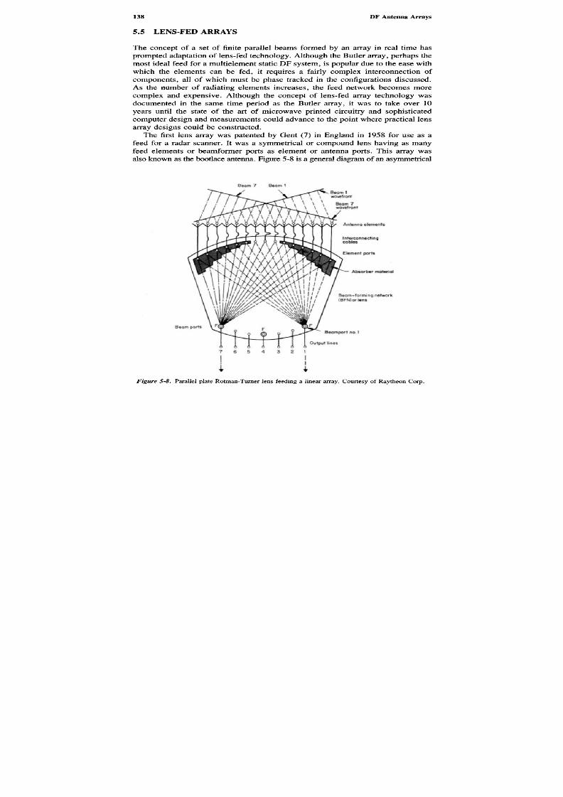
8/8/2019 SciTech - Microwave Passive Direction Finding
http://slidepdf.com/reader/full/scitech-microwave-passive-direction-finding 152/323
5.5 LEN S-FED ARRAYS
The concept of a set of finite parallel beams formed by an array in real time hasprompted adaptation of lens-fed technology. Although the Butler array, perhaps themost ideal feed for a multielement static DF system, is popular due to the ease withwhich the elements can be fed, it requires a fairly complex interconnection ofcomponents, all of which must be phase tracked in the configurations discussed.As the number of radiating elements increases, the feed network becomes morecomplex and expensive. Although the concept of lens-fed array technology wasdocumented in the same time period as the Butler array, it was to take over 10years until the state of the art of microwave printed circuitry and sophisticatedcomputer design and measurements could advance to the point where practical lensarray designs could be constructed.
The first lens array was patented by Gent (7) in England in 1958 for use as afeed for a radar scanner. It was a symmetrical or compound lens having as manyfeed elements or beamformer ports as element or antenna ports. This array wasalso known as the bootlace antenna. Figure 5-8 is a general diagram of an asymmetrical
Beam 7 Beam 1Beam 1wavefront
Beam 7wavefront
Antenna eements
Interconnectingcables
Eement ports
Absorber material
Beam-formng network(BFN)orlens
Beam portsBeamport no. 1
Output lines
Figure 5-8. Parallel plate Rotman-Tumer lens feeding a linear array. Courtesy of Raytheon Corp.

8/8/2019 SciTech - Microwave Passive Direction Finding
http://slidepdf.com/reader/full/scitech-microwave-passive-direction-finding 153/323
lens structure that has a different radius of curvature for the beamformer and an tennaelement ports. Seven beamformer ports and 15 element or antenna feed ports areshown. Each element port is connected to an antenna mounted in-line and connectedto the lens by an interconnecting cable of a different physical length. Rotman andTurner (8) in 1963 described the operation of this type of lens in detail. Theiroriginal design used a parallel plate air dielectric pillbox structure for the lenselement, which was capable of supporting the TEM mode of radiation. The beam-forming ports consisted of radiating horns mounted at one end, which was a circulararc. RF probes at the element end fed a linear array as shown.
Conceptually, the Rotman lens works by summing or focusing N in-phase samplesof a wavefront at a focal point. In Figure 5-8, consider the wavefront from beam1. Each antenna element reading from left to right samples this wavefront at aslightly different time due to its angle of arrival with respect to the plane of theantenna elements. Each interconnecting cable between the antenna elements andthe element ports is adjusted in length such that for three discrete angles of arrival,all signals add up in time at three focal points, shown asF at beam ports 1,4, and7. Tracing the left-most sample of wave front 1 to port 7 and comparing it to theright-most sample at the same port, it may be seen that the electrical path lengthsare all equal due to the carefully adjusted lengths of the interconnecting cables. Asa result, there will be a maximum at port 7 for beam 1. Similarly, if another wavefront, beam 7, for example, arrives at a different angle, there will be a maximumat the focus at beam port 1. A third focus point is available at beam port 4. Anyinput wave front therefore will add up with a maximum at one port from 1 to 7,depending upon the angle of arrival of the corresponding wave front, and detectionof the port amplitude will be a measure of the arrival angle. Although there areonly three focal poin ts, in practice the departure from exact focus at the other beam -former ports is not significant, in a good design, and all ports can be used to make
accurate measurements.Originally designed to be switch selected, the output beam ports may be paralleldetected, resulting in simultaneous parallel formation of beams in a manner similarto a planar Butler-fed array. This is desirable for passive direction finding since theamplitude ratio of beams or the amplitude ratio of a beam to an omniazimuthalantenna will give a monopulse ratio. For retrodirective applications, the RF outputsof one lens array are not detected but are amplified by as many TWT amplifiers asbeamformer ports. The TWT outputs are fed to a similar transmitting lens and
antenna array. Since the array is linear, it follows the reciprocity theorem and abeam will be formed in the transmit array that w ill be the sum of all the TW T 'spower added in space and radiated in the same direction from which the originalsignal arrived. This retrodirectivity is the basis of many jammer designs, the advantagebeing that the total ERP is the sum of many lower-power devices, as opposed toa single high-power device. Redundancy is excellent since failure of one tube willnot disable the system (see Section 4.7).
Since the addition at the focal points is due to equal phase path length for awave front that arrives at a slightly different time at each antenna element, theRotman lens can be considered to be a true time-delay m ultiple beamformer, similar

8/8/2019 SciTech - Microwave Passive Direction Finding
http://slidepdf.com/reader/full/scitech-microwave-passive-direction-finding 154/323
to the Blass matrix (9). In Blass's design (Fig. 5-9), a linear array is fed by a seriesof transmission lines that cross another series effectively perpendicular to the first.At each junction point, there is a direction coupler to isolate the beams. The pathlengths are adjusted to provide the same phase length from each antenna to eachfeed port, resulting in the same time delay. The patterns formed are shown in thefigure and exist in space simultaneously. Since the Blass design (circa 1960) wasexecuted in waveguide, it was dispersive (frequency sensitive) and troubled withdelay-time formation that did not allow short pulses to sum instantaneously. Theconcept, however, was that of a time-delay array, of which the Rotman-Turnertype is a prime exam ple. The great advantage in a Rotman lens is the wide bandwidthand constant beam position attainable. This is due chiefly to the use of the TEMor coaxial modes of propagation for which the phase velocity is nondispersive. TheRotman lens is a true time-delay scanner that can be used either for receiving ortransmitting.
The original Rotman-Turner version of the Gent bootlace lens was made up ofa series of different-length coaxial cab les. A t one end the cables were terminatedin a linear outer surface connected to an array of antenna elements. The other endof the set of different-length coaxial lines was connected to a parallel-plate sectionof maximum thickness terminated at the right by probes connected to the coaxial
cables and at the left by horns or probes, constituting a set ofF^ beam-formerports, of which Fi, Gi, andF^ were in focus. Figure 5-10 shows the geometry of
Antennaarray
0= Directionalcoupler
Figure 5-9. Blass equal length beam-former array.

8/8/2019 SciTech - Microwave Passive Direction Finding
http://slidepdf.com/reader/full/scitech-microwave-passive-direction-finding 155/323
Case for R = F
Figure 5-10. Geometry of the Rotman lens.
the lens. These points were connected by a circular arcR. A signal from an inputwave front arriving at an angle a at element N traveled a phase lengthw throughcable, exited the cable atP x,y , and traveled to the focus port through a ray path inthe parallel plate section.
Archer et al. (10) improved the concept shown by introducing a dielectric m aterial
for air in the parallel plate section (constant C1) reducing the dimensions of thissection by l /V ^ i . This improvement also permitted the use of microstrip andstripline microwave printed circuit techniques to construct the feed section, eliminatingthe probes in favor of printed circuit launchers at the ports, with more determinableVSWRs.
The method of solution of the equations as outlined by Rotman is to choose a,normalize all values to F, the focal length, and determine the coordinates of thebeam former and outer lens contour points. From this, the focal arc center can becomputed. The distortion from the circular arc (phase error) is minimized by choos-ing g = GIF = 1.137 as a comm on value.
Outerlenscontour
Innerlenscontour
Focalarc(circular)
Cables
W
av
font

8/8/2019 SciTech - Microwave Passive Direction Finding
http://slidepdf.com/reader/full/scitech-microwave-passive-direction-finding 156/323
There are only three degrees of freedom: the cable lengthw and the X, Ycoordinates of each pointP of the inner lens contour. The equations for the lensdesign are tabulated as follows:
X W N* = - w = — n = -
F F FY G
y = F g = F
then
y = n{\ - w)
2w(l - g) - b2on
2
2g ~ a0
-b - Vb2 - Aacw =
2a
b = U 8(I^) - ^% bW + ^ - 2,1L \ r aj (g - a0) J
c = \iftL - W - ,2]U ~ ao 4(g ~ G o )2 J
wherea o = cos a
Z?̂ = sin a
R, the radius of the focal arc, lies at the center of atR - G:
= (Fa 0 - G)2 + F2frg2 (G - Fa 0)
Since the above equations derived by Rotman used an air dielectric (G = 1), itis necessary to modify them for a finite dielectric by multiplication ofX and Y by1/V ej- The above equations may be readily solved for the general case with apersonal computer using the program ROTMAN presented by Pozar (11) or for the
symmetrical case as presented by Shelton (12).

8/8/2019 SciTech - Microwave Passive Direction Finding
http://slidepdf.com/reader/full/scitech-microwave-passive-direction-finding 157/323
The Rotman lens has assumed significant importance in naval electronic warfare(EW) systems as a result of the extensive work undertaken to reduce it to a small,reliable format by the Raytheon Corp. Goleta, CA. This has been accomplishedby filling the parallel plate section with high dielectric materials wither varyingfrom 2.3 for Duroid Teflon fiberglass printed circuit material, to e = 233 forcadmium titanate material. Etched microstrip circuits on a barium tetratitanate(e = 38) ceramic substrate are also used . Figure 5-11 is a photograph of a Raytheon66 element linear array fed by a 66 by 18 element beam-port lens. The azimuthpatterns are shown in Figure 5-12a. There is about a 2 dB variation in pattern gain,which varies approximately as the cosine of the scan angle over a 120 degree fieldof view. Each pattern is 5 degrees wide at— 3 dB, down broadening as the secantof the scan angle; backlobe levels are down by 24 dB. The elevation pattern (Fig.5-\2b) is approximately 10 degrees. The Rotman lens can also be used to feedmoderately curved arc arrays. This is desirable for conformal applications. Figure5-13 is a photograph of a 45 degree arc antenna covering 120 degrees that operatesover a 2.5:1 frequency band. A four-sheet meander-line polarizer that convertscircular and linear polarized signals to the linear polarization of the array is shown.This type of antenna offers improvement in gain roll-off at the extremes of angularcoverage and can operate over wider RF bandwidths.
It is not feasible to use Rotman lens and linear or arc array to cover a full 180or 360 degree azimuth angle since there is increasing rolloffin the contiguous beam sas the angular sector is increased. A circular lens, however, known as the R-KR(13), may be used in a similar manner to develop semicircular contiguous beams.The lens diameter isK times the diameter of the array, whereK is usually optimizedat 1.9. Equal-length cables connect the antenna elements to the lens. Figure 5-14is a photograph of a 17-element circularly polarized hemispherical azimuthal coverageantenna that operates over a 2.4:1 frequency band. Figure 5-15 shows the patterns
obtained by this antenna. This type of array can be configured to cover 360 degrees
Figure 5-11. A 66-linear element array fed by a 66 x 18 beam-former len s. Courtesy of Raytheon
Corp.

8/8/2019 SciTech - Microwave Passive Direction Finding
http://slidepdf.com/reader/full/scitech-microwave-passive-direction-finding 158/323
(b)
Figure 5-12. (a ) Patterns of a linear 66 x 18 beam array,(b) Elevation (Q H)pattern of 66 x 18 beamarray. Courtesy of Raytheon Corp.
RELATIVEPOW
ER dB)
(a)

8/8/2019 SciTech - Microwave Passive Direction Finding
http://slidepdf.com/reader/full/scitech-microwave-passive-direction-finding 159/323
Figure 5-14. The R-KR hemispherical multibeam lens-fed array. Courtesy of Raytheon Corp.
Figure 5-13. A 45 degree arc array fed by a stripline Rotman lens covering 120 degrees of azimuth.

8/8/2019 SciTech - Microwave Passive Direction Finding
http://slidepdf.com/reader/full/scitech-microwave-passive-direction-finding 160/323
Figure 5-15. Patterns of the R-KR hemispherical multibeam lens-fed array. Courtesy of Raytheon Corp.
by interconnecting two lenses together with broadband 90 degree hybrids as shownin Figure 5-16.
The circular array features constant beam width patterns as a function of the scanangle, which is highly desirable. The maximum elevation angle coverage is
e m a x = 2 0 2 y |
where
D/X = the array diameter in wavelengths
The antenna horizontal beamwidth is
59X* = ~^
This places a practical limitation on large diameter arrays since they will nothave wide vertical beamwidth coverage. The Rotman lens as modified by Archer,Monser, and others at Raytheon has been chosen as the standard U.S. Navy electronic
support and countermeasures (ESM/ECM) suite and is finding wide application inthis role as well as in airborne and other applications. It has taken many years andmuch effort to convert the early Gent bootlace lens into a practical multibeam array.

8/8/2019 SciTech - Microwave Passive Direction Finding
http://slidepdf.com/reader/full/scitech-microwave-passive-direction-finding 161/323
Figure 5-16. Omniazimuthal multibeam array utilizing two 90 degree hybrid interconnected R-KRlenses.
5.6 PARALLEL BEAM SEPTUM ANTENNA
In certain app lications, it is necessary to develop direction-finding systems that canoperate in limited space with elements that are not able to have sufficient aperture
to attain high gain. These types of applications are generally found in aircraftinstallations and where space is at a premium. It is instructive to consider a ratherunusual configuration provided by a corner reflector type of antenna, designed bythe Elisra Corp., to cover an 8:1 frequency range at reasonable gain levels, withgood DF accuracy.
Figure 5-17 is a photograph of a CD-L-band corner reflector antenna with itsradome removed to show details. This antenna covers . 5 - 2 G Hz and provides three
Figure 5-17. Three-element multibeam septum antenna. Courtesy of Elisra Corp.
Beamport Beamport
Antelement
Circular lens I
Circular lens 2
Antelement
51

8/8/2019 SciTech - Microwave Passive Direction Finding
http://slidepdf.com/reader/full/scitech-microwave-passive-direction-finding 162/323
unambiguous parallel beam outputs from three corner reflectors spaced 120 degreesapart. Each radiating element is a printed circuit broadband inverted-T sectionterminated at the far end. The center of the T is fed directly by a coaxial cable atthe input port. The vertical members are fed from the center point and are terminatedby resistive material to reduce reflections. The corner reflector is a three-piecetriangular conducting septum grounded at the base plate. The 120 degree angleformed between the vertical members and the 90 degree angle formed by the septumand the baseplate tend to point the peak of the resulting beam downward; and sincethe antenna is mounted at the front underside of an aircraft, //-plane coverage (9)is from the horizon to - 4 5 degrees with the aircraft acting as a ground plane. Asingle cylindrical radome encloses the antenna.
Figures 5-18 and 5-19 are patterns taken at 700 and 1800 MHz at an elevationangle of -22° below the horizon degrees for a vertically polarized source. At 700M Hz, crossover occurs at - 3 dB points with a beamwidth of 220 degrees; at 1.8GHz beam crossover occurs at 3.6 dB at 180 degree beamwidth. The gains of the
Figure 5-18. Parallel beam three-element septum antenna—0.7 GHz patterns.
Angle

8/8/2019 SciTech - Microwave Passive Direction Finding
http://slidepdf.com/reader/full/scitech-microwave-passive-direction-finding 163/323
Figure 5-19. Parallel beam three-element septum antenna—1.8 GHz patterns.
antenna are listed in Table 5 -1 . The gain increases with increasing frequency, whichcan be compensated for by active RF amplification if required. DF determinationis made by an amplitude comparison monopulse comparator. The absence of strongback lobes and the fairly predictable crossover levels permit a DF accuracy to beobtained to at least octant accuracy over the frequency range. The septum antennaapproach can be extended to a greater number of elements and can be used with a
Butler-feed network since the absence of backlobes indicates relatively good isolationbetween the elements.
Table 5-7. Septum Antenna Gain Characteristic
Frequency (GHz) Gain (6 = -2 2 ° ) (dBi)
• 0 .5 - 8
1.0 +3
1.5 +52.0 +6
Angle

8/8/2019 SciTech - Microwave Passive Direction Finding
http://slidepdf.com/reader/full/scitech-microwave-passive-direction-finding 164/323
5.7 SWITCH ED-BEAM ARRAYS
In many DF app lications, it is not necessary or desirable to cover a full 360 degreesof azimuth. For example, in a situation where an ELINT aircraft is located at somedistance from the expected targets, the basic direction-of-arrival of all desired signalsis approximately known; what is needed generally is range and high precision. Ingeographic situations where the presence or turn on of radar emitters is to bedetermined, a sector DF system may be adequate. Although it is obvious that anyof the multibeam approaches described thus far can be switched to selectively covera given sector or beam in a planar sector, the advantage of attaining all of the arrayfactor gain is not achieved if the unused ports of the switched multibeam must beterminated. From a transmit point of view, a switched-array that provides full arrayfactor gain is highly desirable since it increases hard-to-achieve effective radiatedpower.
Switched-antenna systems are not commonly used with passive DF receiversdue chiefly to the restricted instantaneous RF bandwidth usually associated withthe feed network and the probability of detection loss resulting from the finiteswitching time. In the study of the Rotman lens system discussed above, switchingcan be used to describe which beam-former port has the maximum signal to determinethe angle of arrival; however, parallel comparison is easier. In a multiple-hornsystem, switching can be used effectively to replace the rotating joint in a m echanicallyrotating antenna system.
In array technology, switching of phase and amplitude increments between variouselements can be used to steer a beam. For missile work, switching of planar arrayswith relatively narrow field-of-views is a highly practical method of accurate DFdetermination, since diode or varactor elements can be used due to the low-powerapplication. Switch-steered arrays are extremely popular in radar work since great
increases of effective radiated power are achieved. In these cases, locking ferriteswitching devices add finite phase element increments to effect power summationof radiation from multielement arrays. Switched-phase lock injection accomplishesthe same result from active element radiators in major systems.
In steered-array systems there are two basic types of effects that have a significanteffect on their use for passive direction finding. Both effects are related to theinstantaneous bandwidth that can be obtained. The first is the obvious limitation ofthe devices used to construct the array; that is, couplers, power dividers, phase
shifters, and so on, each of which is imperfect to some extent. These effects arepredictable. The second effect is due to the repeating nature of wavelength associatedstructures such as stubs, waveguides, and varying lengths. Only 2ir or 360 degreesof phase change can be obtained in effect, and the rate at which it can be madeuseful depends upon distances between elements.
In actuality, a phased array would like to excite all radiating elements at thesame time, with different phase and amplitudes at each of the elements to achievedirectionality. The extent to which this can be accomplished varies with the con-figuration. A Rotman lens is a true time-delay phase shifter as are the Blass andother similar configurations. The characteristics of this class of device is beam

8/8/2019 SciTech - Microwave Passive Direction Finding
http://slidepdf.com/reader/full/scitech-microwave-passive-direction-finding 165/323
pointing accuracy that is independent with frequency. Butler matrixes are not time-delay devices; however, if thedifferential phase shift is made directly proportionalto frequency, the beam(s) will continuously point in one direction over wide bandwidths.The combination used for the circular array as described previously exhibits thisproperty as a result of the choice of radiation and diameter and is a good exampleof which broadband circular arrays are often fed by the Butler matrix.
Steered-receive linear arrays have been developed utilizing phased-array techniquesdespite the above limitations. A planar steered-beam system is shown in Figure5-20 and described in Ref. 14. In this case, a group or set of linearly alignedantennas is combined in series with a programmable phase shifter to apply a progressivetime delay to each section permitting the formation of the two scanned beams.These two beams are combined in a S - A hybrid to form an amplitude signal pairthat is subtracted to provide the angle of arrival c> as a function of the settings ofthe phase shifters, which are essentially scanned. The superheterodyne receiver isalso tuned adding a second scanning probability to the detection process. It isclaimed, however, that sensitivities of —70 dBm or greater can be achieved withthis technique, exclusive of the antenna array gain. The DF accuracy is in the orderof 1/30 of a beamwidth, the advantage of the system being the potential for fulldigital control and frequency correction.
There have been several attempts to design circular switched-phased arrays toreplicate the scanning action of a rotating DF antenna. An early attempt by the
Antenna array
Phaseshifters
Phasesteeringcontrol
Localoscillator
LogIF
TuneSub tractor 0Output
LogIF
Figure 5-20. Azimuth scanning beam passive DF receiver.

8/8/2019 SciTech - Microwave Passive Direction Finding
http://slidepdf.com/reader/full/scitech-microwave-passive-direction-finding 166/323
U.S. Navy (15) resulted in the configuration shown in Figure 5-21. The conceptwas to make use of the circular array since, as described previously, the symmetryof the array is the same due to a constant relative phase shift between all elements.The antenna reportedly achieved 128 beam positions, with a crossover at - 2 dB ,a half-power beam width of 4 - 5 degrees, and a side-lobe level of 25 dB . Each stepmoved one element and was computer-controlled. The radiating elements werewaveguide sectioned horns spaced at 0.65 wavelength in a cylinder of a 13.2wavelength radius . AU cables connecting the radiating horns were of equal electricallength. The phase shifters were PIN diode types and were followed by a programmableamplitude attenuator to vary the taper to control backlobes. The system achieveda 20% instantaneous bandwidth. In a later configuration, a R-2R lens similar to thetype described for the Raytheon multibeam design, was used to eliminate the phaseand amplitude switching by phase focusing through the action of the lens.
The above approaches, although somewhat complex, have been simplified bythe availability of the frequency word from an instantaneous frequency measurement(IFM) or digital frequency encoder. As a result, future switch-scanned arrays maybe developed to actually reduce the cost of the RF section of a DF receiver by theuse of less expensive digital encoding storage and connection methods. The trendis clear for the transmit side, where high effective radiated power is obtained more
inexpensively by a multiplicity of amplifiers and radiating elements, w ith the addedadvantage of redundancy and reliability. The need for higher sensitivities can bebest achieved by narrower steered DF beam antennas, where high instantaneousintercept probability is not required.
5.8 SUMMARY
This chapter has covered the important phased array antenna systems used in modernelectronic warfare passive direction finding systems. The groupings have beencharacteristically divided into the way the detection problem stands—multiplecoverage or parallel beam antennas for maximum spatial intercept probability ver-sus switched-beam techniques for higher accuracy and greater effective antennagain—at the price of a detection probability due to the required scanning process.Both types of systems are in use. The third system, the interferometer, will bedetailed in Chapter 6; however, it may be seen that this approach is, in effect, aform of both types of the antennas presented here.
It is important to note that phased-array DF systems lend themselves readily toconformal antenna arrangements where the vehicle is enclosed by the antennasystem. Since the performance of an array has more antenna elements, it is moretolerant of perturbations than say a four-element system and is therefore capableof better accuracy under many conditions. It is also possible to reduce the cost ofreceive arrays by the use of printed circuit radiators and feed netw orks, which allowthe array, with all of its apparent circuit complexity, to be reduced to relativelyeasy-to-manufacture assem blies. Arrays become costly as they are required to handlepower, the receiver arrays becoming more practical as feed networks improve.

8/8/2019 SciTech - Microwave Passive Direction Finding
http://slidepdf.com/reader/full/scitech-microwave-passive-direction-finding 167/323
d i v i d e r
S P 4 TB it
0 a a m p l
Figure 5-21. A 128-element switche

8/8/2019 SciTech - Microwave Passive Direction Finding
http://slidepdf.com/reader/full/scitech-microwave-passive-direction-finding 168/323
For these reasons, the topic of DF antenna arrays has been given more attentionthan current usage would imply. As higher frequency millimeter wave technologyevolves, the phased array is certain to play an important part in passive directionfinding for missiles, remotely piloted vehicles, and spaceborne vehicles due to thesmaller sizes achievable.
R E F E R E N C E S
1. Steinberg, B. D.,Principles of Aperture & Array System Design,New York: Wiley, 1976, p. 76.
2. Butler, J., and R. Lowe, "Beam Forming Matrix Simplifies Design of Electronically ScannedAntennas," Electronic Design 9, 1961, pp. 1 70 -17 3.
3. Hansen, R. C , Ed., Microwave Scanning Antennas,New York: Academic Press, 1966, Vol. Ill,p. 260.
4. Sheleg, B., "A Matrix-Fed Circular Array for Continuous Scanning,"Proc. IEEE, Vol. 56, No.11, Nov. 68.
5. Shelton, P., "Application of Frequency Scanning to Circular Arrays," IRE WESCON Conv. RecordPt. 1, 1960, p. 83.
6. Cha dwick , G ., and J. Glass, "Investigation of a Mu ltiple Beam Scanning Circular A rray," Report1—USAF Cambridge Research Lab, Cambridge, MA, Contract AF 19/628/367, Dec. 1962.
7. Gent, H., "The Bootlace Aerial,"Royal Radar Establishment Journal, England, Oct. 1957, pp.4 7 - 5 7 .
8. Rotman, W., and R. Turner, "Wide-Angle Microwave Lens for Line Source Applications,"IEEEAP-T, Nov. 1963, p. 623.
9. Blass, J., "M ulti-Directional Antenna — A New Approach to Stacked Beam s,"IRE National ConventionRecord, 1960, Part 1, pp. 48-50.
10. Archer, D., R. Prickett, and C. Hartwig, "Multi-Beam Array Antenna," U.S. Patent 3,761,936,Sept. 25, 1973.
11. Pozar, D., "Antenna Design Using Personal Computers," Dedham, MA: Artech House, 1985,p. 94.
12 . Shelton, J. P., "Focusing Characteristics of Symmetrically Configured Bootlace Lenses," NRLMemorandum Report 3483, April 1977, ADA 039843.
13 . Thies, W., Jr., "Omnidirectional Multibeam Antenna," U.S. Patent 3,754,270, May 1974.
14. Simpson, M., "High ERP Phased Array ECM Systems,"Journal of Electronic Defense, Mar. 1982.
15. Boyns, J., "Step Scanned Circular-Array Antenna," Phased Array Conference, 1977.

8/8/2019 SciTech - Microwave Passive Direction Finding
http://slidepdf.com/reader/full/scitech-microwave-passive-direction-finding 169/323
InterferometerDF Techniques
Interferometers can be considered specific cases of array antennas. The linear arrayin which all antenna elements center lie in a straight line at equal spacings withbeam forming done by phase shift networks is an example. In an interferometer,the elements can also lie in a straight line but are usually at different spacings toobtain time-of-arrival relationships that can be transposed into measurable phasedifferences for determination of angle-of-arrival information. The concept alsoextends to the circular array, where interferometer techniques can be applied toalso cover 360 degrees of azimuth from an antenna mounted at one point.
In Chapter 2 , Section 2 .2 1 , the simple interferometer antenna system was described
as a DF measurement technique based upon the difference of the time of arrival ofa signal detected by two identical collocated antennas in space separated by a finitebase line. It was shown that the output of the antennas differed in phase from eachother in proportion to the extra time it took a plane wave signal to travel a greaterdistance to the further antenna. Since a signal would be detected at the same timeif it were equally displaced from both antennas, the phase difference would be ze ro,creating a phase difference null along the boresight for this condition. The measurementof the time difference or phase, whenever it is greater or less than zero, therefore,
can give the incoming angle with respect to boresight.A DF system consisting of two monopulses in space is 180 degrees ambiguoussince it is not clear from which half of the hem isphere the signal originated. Practicalinterferometer systems solve this problem by using another system such as anamplitude monopulse DF to select the proper direction, or use quadrant arrays ofantennas shielded from each other, or a circular array of monopoles to unambiguouslycover a 360 degree field of view. In the first technique, ambiguity resolution isobtained by shielding , which is accomplished by utilizing an artificial ground plan e,
such as the side of a ship or plane, to absorb or reflect the back wave. The lastmethod resolves the ambiguity by measuring the relative differences in phases
Chapter Six

8/8/2019 SciTech - Microwave Passive Direction Finding
http://slidepdf.com/reader/full/scitech-microwave-passive-direction-finding 170/323
between all the radiating elements around a circle, essentially resolving ambiguousresponses.
Wide frequency coverage is generally desired in interferometer systems used forpassive detection, necessitating that more than one set of antennas and more thanone fixed baseline between the antennas be used, since the solution of the angle-of-arrival equations for a single baseline system is not single valued. Interferometersof this type are called multiple baseline types and generally consist of a referenceantenna in the center of two or more other antennas spaced in line and at differentdistances from it. It is possible to use many baselines and antennas to obtain widefrequency coverage. By relating the baselines in a known manner or by using theknown RF frequency in the processing, all DF ambiguities can be resolved (1). Inanother technique the phase spacing can be made proportional to frequency bypointing two conical antennas toward each other. In this case the phase null ambiguityis resolved since the spacing optimizes itself for each frequency. The wide bandw idthof conical spirals makes this a useful technique (2). In this chapter we shall considerseveral forms of the multiple baseline interferometer with both sectorized linearand circularly dispersed elements. Examples of the system configurations of bothtypes will be given to show typical applications for dispersed and single-pointantennas.
6.1 MATHEM ATICS OF INTERFERO ME TRY
At the outset, it is important to understand that the antenna part of interferometersystems is almost always a phase m onopulse configuration, permitting the processingtechniques outlined in Chapter 2 to apply. The practical problem of measurementof phase, however, often requires that combinational phase and amplitude systemsbe used. An example of this is the resolution of previously mentioned ambiguity:
By detecting the antenna amplitude as well as phase responses and by comparingsectors in an amplitude monopulse system, it is possible to eliminate the multipledirectional null am biguities of the phase interferometer that occur when frequencieshaving wavelengths less than the minimum unam biguous spacing (X/2) of an antennapair are present.
In Figure 6-1 ,the single baseline two-antenna interferometer has been drawn toshow operation in the first quadrant. The voltage received by antenna 2 may be
Input signal
Figure 6-1. Single baseline interferometer.

8/8/2019 SciTech - Microwave Passive Direction Finding
http://slidepdf.com/reader/full/scitech-microwave-passive-direction-finding 171/323
expressed in exponential form as follows:
V2 = VexJjut -YX) (6"1}
where
V = the initial transmitted signal amplitude
X = the distance traveled
2TT/\ = free space propagation constant
and in a like manner at antenna 1:
( 2 \
jut X + D cos <() I (6-2)^ /
where the term D cos <\> represents the additional path length to antenna 1 asreferenced to antenna 2 . Since we are interested in relative phase differences betweenthe two received voltages, Vi and V2, we can assume (2u/\)X to be reference zero
at antenna 2; then,V2 = e*"' (6-3)
and
Vi = explycof + —D cos $) (6-4)
Taking the natural log (In) of both sides of the equation and subtracting to obtainthe difference voltages yields
V2
In V2 - In Vi = In — = ycof - pit + JD cos c() (6-5)^ i
= j - ^ D cos <> (6-6)\
Let Mf be defined as this difference or the real part of Equation (6-5); then ,
AM' = — D cos <> (6-7)A.
Taking the difference of the two natural log voltages effectively forms the ratioIn V2/Vi, which m akes this interferometer a phase monopulse system; the AM' termhas been normalized with respect to input signal variation and is the monopulseratio.

8/8/2019 SciTech - Microwave Passive Direction Finding
http://slidepdf.com/reader/full/scitech-microwave-passive-direction-finding 172/323
Substituting
A^F = - , where c = 3 x 1010 cm/sec
and solving Equation (6-7) for cos cj) in terms of frequency yields
3 0 A ^
c o s • = 2^f (6" 8)
where
AW = the phase difference in radians (2ir radians = 360 degrees)
/ = the frequency of the intercept expressed in gigahertz per second
D = the spacing measured in centimeters
c j> = the angle of arrival
or
A ^cos c)) = ^ - (in degrees) (6-9)
Since A^P repeats itself every 360 degrees for all higher frequencies where theincoming wavelength is less thanD, for the cos cj> in Figure 6-1 to be unam biguous,the relative phase shift A1P must be
0 < A^F < 360 degrees (6-10)
For the general case, then
. A ^ + 360*:CO S » = 12/D ( 6 - U )
where K is any positive integer that is the solution number corresponding to higherfrequencies. Since the cosine is always less than 1, K is limited to only those valuesthat make cos 4> ^ 1 in Equation (6-11).
The two-antenna interferometer is therefore a limited bandwidth device since ifthe RF bandwidth is extended higher, a greater number ofK solutions will resultand it will be impossible to know whichK is correct.
This can be shown by rearranging terms in (6-11):
A ^ + ITTK
co s <> = — (6- 12 )

8/8/2019 SciTech - Microwave Passive Direction Finding
http://slidepdf.com/reader/full/scitech-microwave-passive-direction-finding 173/323
Substi tuting/ = B/X, where B contains all constants, and dividing by 2 gives
B - cos (f> = — + K (6-13)
X Z1TFigure 6-2 is a plot of c|>, the angle of arrival (as measured from the horizon 0-90degrees in the first quadrant) as a function of( A ^ / 2 T T ) + K.
From the plot it may be seen that there will be no ambiguities for D/X= Vi. Ifwe consider any other spacing to wavelength ratio such as D/X= 4, for example,for a change from 10 to 80 degrees, there will be a change in (A^/2Tr) +K from3.6 to .5 or 3.1 degrees of. rotation, creating three am biguities. The single base-
line system would therefore not be single-valued over this span.Consider, however, the articulation, which for an interferometer can be definedhere as rate of change of angle of phase for angle of arrival. If we define the slopemo.5 to be that of the D/X = Vi, then
.5 180 degreesx = .32 degree/degree
90 degrees ir(rad) B B
For D/X = 4, the slopem4 for this case is
4 180x = 2.55 degree/degree
90 degrees TT
which is eight times better than D =Vi (4/.5) as expected; therefore, it is possibleto conclude that the interferometer D F technique can achieve very high resolutionby a choice of largeD/X ratios at the expense of solving the ambiguity problem
Figure 6-2. Interferometer ambiguity (A^/2TT + K) as a function of the angle of arrival and spacingto wavelength of a single baseline interferometer.
<f> (Angle of arrival)
2TT

8/8/2019 SciTech - Microwave Passive Direction Finding
http://slidepdf.com/reader/full/scitech-microwave-passive-direction-finding 174/323
Angle of arrival
Figure 6-3. Ambiguity resolution in a multiple baseline interferometer.
that will result.This is the basis for the use of this technique in high resolution DFsystems.
One method of resolving the ambiguities over a limited frequency range is tolimit the field-of-view of the antenna. Another method is to use a multiple base-line. Figure 6-3 shows the latter concept: An ambiguous baseline pair gives rise toambiguities Kx, K2, K3, and K4 (solid line), which can be resolved by another
baseline pair (dotted line) having no ambiguities, the second pair being m ore closelyspaced. The fine angular measurement is best measured by the widest space pairsince it has the greatest articulation (phase change per degree); however, the mostsignificant number for the measurement, the unambiguous one, is made by thechannel with the least articulation, requiring a better signal-to-noise ratio in thischannel to provide accuracy. An amplitude-measuring system is often used here toprovide this resolution if a signal-to-noise advantage exists.
Figure 6-4 show s a dual baseline system w here antenna 1 is spaced at a distance
D1 from antenna 2 forming a short baseline interferometer, while antenna 3 isspaced at a distanceD2 from antenna 1 forming a long base-line interferometer.
In the first quadrant, V3 lags V2, which lags V1. Equation (6-11) rewritten forthis case becomes
A ^ 1 + 3 6 0 ^1
cos eh = — — (6-14)
A ^ P2 + 360/T2cos c()2 = — — (6-15)YIjD2
R
esolver
output
volage

8/8/2019 SciTech - Microwave Passive Direction Finding
http://slidepdf.com/reader/full/scitech-microwave-passive-direction-finding 175/323
where
D 1 * D2
For a given range of frequencies, the values ofKx and K2 can be computed bysetting cos (J)1 and cos <|>2 equal to unity and solving forK. For example, usingEquation (6-14)
. A^P1 + 36OZf 1
c o s * = — I 2 / D T ~ ~ * 1
Then
A ^ + 360K 1 ^ 12/D1
but
A ^ = 0
360K1 = YIfDx
K ~fD l
a. 0< <t> <9O (Quadrant I)Ant 3 Ant I Ant 2
b. 90<<fi'< 180 (Quadrant II)Figure 6-4. Dual baseline interferometer, (a ) Quadrant I, where 0 ^ <J> «£ 90 degrees ,(b) QuadrantII, where 90 ^ <\> ^ 180 degrees .
Ant 3 Ant I Ant 2

8/8/2019 SciTech - Microwave Passive Direction Finding
http://slidepdf.com/reader/full/scitech-microwave-passive-direction-finding 176/323
K\ can have multiple values for higher frequencies as before (seeDfK curves inFig. 6-2). The number of ambiguities will be an integer ranging from zero, theideal case, to any integer less than the solution.
In quadrant II the angle of arrival becomes a lead angle; that is, V3 leads V1,which leads W1- This is shown in Figure 6-42?.
At 90 degrees or boresight there is no differential angle and the angle-of-arrivalreverses from lag to lead. Since most real-time measuring systems measure the lagangle, some adjustment to the equations is required. Defining quadrant II valuesas primed, and measuring them as shown, Equation (6-9) becomes
A d/cos cp1 = " - ^ (6-16)
A ̂ ' is a lead angle now and is therefore negative with respect to the m easurementsystem. Figure 6-5 shows the quadrant relationships. The signal arriving at (J)1 inquadrant II would have the same value asCOS(TT - cj>) for an equivalen t in quadrantI where
TT/2 < ct)1 ^ TT
cos tyl = COS(TT - 4>)
= c o s TT c o s (j> + s inTT s in cf>
= —cos4>
c o s * = ^ 5 (6-17)
Quadrant
Figure 6-5. Quadrant relationships for the dual baseline interferometer.
Cosinefunction
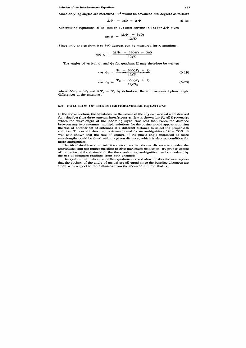
8/8/2019 SciTech - Microwave Passive Direction Finding
http://slidepdf.com/reader/full/scitech-microwave-passive-direction-finding 177/323
Since only lag angles are measured, NP1 would be advanced 360 degrees as follows
A ^ 1 = 360 + AV (6-18)
Substituting Equations (6-18) into (6-17) after solving (6-18) forAV gives
(AV1 - 360)C 0 S * = XIfD
Since only angles from 0 to 360 degrees can be measured forK solutions,
(A V1
- 360K) - 360COS(f) = WbThe angles of arrival (f>i and cj>2 for quadrant II may therefore be written
V1 - 360(^1 + 1)cos Cf)1 = - 1 - — ^ '- (6-19)
V1 - 360(/T2 4- 1)cos c|)2 = - 1 — ^ }- (6-20)VlJU 1
where AVx = Vx and AV1 — ^i by definition, the true measured phase angledifferences at the antennas.
6.2 SOLUTION OF THE INTERFERO ME TER EQUATIONS
In the above section, the equations for the cosine of the angle-of-arrival were derivedfor a dual baseline three-antenna interferometer. It was shown that for all frequencieswhere the wavelength of the incoming signal was less than twice the distancebetween any two antennas, multiple solutions for the cosine would appear requiringthe use of another set of antennas at a different distance to select the properKthsolution. This establishes the maximum bound for no ambiguities ofK = 2DI\. It
was also shown that the rate of change of the phase angle increased as morewavelengths could be fitted within a given distance, which is also the condition formore ambiguities.
The ideal dual base-line interferometer uses the shorter distance to resolve theambiguities and the longer baseline to give maximum resolution. B y proper choiceof the ratios of the distance of the three antennas, ambiguities can be resolved bythe use of common readings from both channels.
The system that makes use of the equations derived above makes the assumptionthat the cosines of the angle-of-arrival are all equal since the baseline distances aresmall with respect to the distances from the received emitter, that is,

8/8/2019 SciTech - Microwave Passive Direction Finding
http://slidepdf.com/reader/full/scitech-microwave-passive-direction-finding 178/323

8/8/2019 SciTech - Microwave Passive Direction Finding
http://slidepdf.com/reader/full/scitech-microwave-passive-direction-finding 179/323
The solution method is to let each A^P be represented by the sum of two phaseangles 1F + W, the first being the quantized va lue, the primed being the independentsystem error. Equations (6-22) and (6-23) can then be expressed in terms of thequantifying increment 360/2, whereQ is the minimum resolution of the encodingsystem. By substituting the known values forR and Q and solving (6-22) and(6-23) for the measured phase differences 1̂ - W2
m terms of K, the systemerrors, and ^ I and W2, it is possible to develop a family ofK numbers, whichwhen compared to the quantum numberQ at various frequencies can provide aunique solution to the interferometer ambiguity resolution. The special case ofA1Fi = A^F2 ^ 0 occurring at system boresight is recognized by the presence ofsignals in both channels at the same frequency while at differential phase zero.
The determination of the angle-of-arrival by interferometer methods will befurther detailed in Chapter 9 discussing accuracy and signal-to-noise ratios; however,it is useful to again point out that the base accuracy and signal-to-noise ratio areachieved by the longest baseline interferometer, which has the highest probabilityof error due to multiple ambiguities yet provides the best articulation. The shortbaseline interferometer gives the poorest signal-to-noise performance but can bemade unambiguous. In a quantized system, the short baseline yields the most sig-nificant digit of the DF measurement and often determines the sensitivity of the system.
The mathem atical details of a two-quadrant planar (in-line) interferometer systemhave been presented above to give the reader a basic idea of how interferometerswork and the significance of the maxim um usable high frequency and the am biguitiesthat result. The derivation method was chosen to show how the details can beworked out since most texts assume that once the concept is presented, the readercan easily proceed to a solution, which is not always the case.
In practical systems, phase-only interferometers suffer from accuracy problems.Although they have the potential for very high accuracy, it is coupled with finite
probability of incorrect ambiguity resolution, called gross error. Although fre-quency-independent systems can be built, knowledge of the intercept frequency isan important tool in reduction of the above error probability. Reference 3 givescurves of probability of ambiguity as a function of the bounds on the ratio of theseparations between the antennas, assuming that the separations are not equal(Di T̂ D2 in Fig. 6-4). It can be concluded that there is a higher possibility forerror. For this reason most interferometers used in passive DF work are designedto be planar multiple antenna sections, conformally dispersed about a host vehicle,and used in conjunction with amplitude comparison techniques. This is done bycomparing the amplitude of each section in a manner similar to that done for afour-spiral DF system as an ambiguity resolving method. W hen conformal mountingcan be replaced by single-point mounting, a cylindrical or multielement Butler-fedarray, or circular interferometer, is used.
6,3 MU LTIPLE-APERTURE SYSTEMS
It is possible to utilize related multiple antenna apertures and multiple baselines inknown ratios to make the determination of the angle of arrival unambiguous over

8/8/2019 SciTech - Microwave Passive Direction Finding
http://slidepdf.com/reader/full/scitech-microwave-passive-direction-finding 180/323
Figure 6-6. Unambiguous multiple baseline interferometer system with binary relationships betweenspacings.
a wide frequency range. Reference 4 describes a binary-beam interferometer systemthat divides each aperture base line by a factor of 2 as shown in Figure 6-6. For abinary variation of 2, between pairs the system is unambiguous from boresight tothe ± 90 degree m aximum field-of-view{K\ = K2 = 0) since the cosine of theangle of arrival is uniquely determinable. The first antenna pair forms a A./2 baselinewith greater slope (articulation) than the next but with ambiguities w hich are resolved
by the next pair. The process continues up to the longest baseline (shown in thefigure).When a signal is received, the entire DF word is defined. The interferometer is
used to remove ambiguities of the2k pair, which rem oves ambiguities of the Xpair, and so on. The resolution can be as great as the number of baselines used.Frequency information can be obtained to provide the means to determine theKnumbers as well as provide intercept frequency.
In a multiple-aperture or baseline system there are two basic choices to be made:
a harmonic binary-related system as described above or a nonharmonic-relatedspaced baseline array. As shown, the harmonic or, in this case, binary systemprovides a completely unambiguous output of DF up to the highest operating fre-quency by the antenna pair relationship. In the nonharmonic system, ambiguitieswill be present at many frequencies; however, knowledge of the spacing ratios andthe frequency of the incom ing signal permits computation by the use of digital look-up tables and logic methods. Any errors or mistrack in the RF receiving systemcan be incorporated into the correction.
The trend in interferometers is toward the nonharmonic type since a greater RFbandw idth coverage can be provided in contrast to the original concept of the binary-type system. This is due to the improvement in instantaneous frequency measure-ment techniques and the fact that, in actuality, both types of interferometers needfrequency corrections and, of necessity, utilize superheterodyne techniques to limitthe instantaneous frequency bandwidth. A binary system is limited on its use at thehigh-end frequency range to the half-wavelength spacing and at the lowest frequencyby physical dimension. In practice, it is claimed (5) that 2-18 GHz coverage can
be provided with nonharmonic spacing, related antennas with 0.1-3 degrees RMSaccuracies.

8/8/2019 SciTech - Microwave Passive Direction Finding
http://slidepdf.com/reader/full/scitech-microwave-passive-direction-finding 181/323
Antennas used for the above systems are generally planar circularly polarizedarchimedian spiral antennas, which are mounted in the baseline surface and rotated,or clocked, to obtain the best phase m atching . S ince the system is a phase monopulsereceiver, amplitude balance is less important, and since the phase variation doublesfor each binary baseline increase, phase matching becomes less critical for thelongest baseline channel.
6.4 LINEAR AND CIRCULAR INTERFEROMETER ARRAYS
An interferometer system making use of many of the concepts presented here isshown in Figure 6
77, a generic four-quadrant DF system patterned after Ref. 6.
This system utilizes four quadrant superheterodyne receivers geographically dis-persed around the host vehicle, each providing coverage of a 90 degree sector. A
Linear orlog ampls
Ampmonopulse
Phasemonopulse
Quadrant
Limiters
Southinterferometer(same for N.,E.aW.)
Angleofarrival
Figure 6-7. Phase monopulse DF receiver with amplitude monopulse ambiguity resolution.

8/8/2019 SciTech - Microwave Passive Direction Finding
http://slidepdf.com/reader/full/scitech-microwave-passive-direction-finding 182/323

8/8/2019 SciTech - Microwave Passive Direction Finding
http://slidepdf.com/reader/full/scitech-microwave-passive-direction-finding 183/323
Figure 6-8. Four-element Butler-fed circular array.
a 90 degree shift with respectto N = ± 1, to a 180 degree shift with respect toN = ±2 and a 270 degree shift w ith respect ton = 1. Table 6-1 shows the ultimateresults for all signals.
By comparing the bearing angleof N = 0 to N = ±1 (the N + 2 and N - 1ports are unused), the phase output will equal the phase input for a 1:1 correspon-dence. Any signal appearing in between the antennas will interpolate. The system
Table 6-1. Phase Relationships at Output PortsNn due to Antenna Inputs atn n
Phase Output at Portn
< $ > AInput Direction N = O W = + 1 N= +2 N = - 1 /i = + I t o O
N (0 degrees) n = 1 0 0 0 0 0E (90 degrees) n = 2 0 90 180 270 90S (180 degrees) n = 3 0 180 0 180 180W (270 degrees) n = 4 0 270 180 90 270
not used
90° PhaseShift

8/8/2019 SciTech - Microwave Passive Direction Finding
http://slidepdf.com/reader/full/scitech-microwave-passive-direction-finding 184/323
is frequency independent and able to operate over a wider range; however, moreelements are needed to improve the discrimination. This is in contrast to the narrow-band, high-precision linear interferometer, which usually requires superheterodynereceivers with matched phase characteristics.
The system described above can be extended into a multielement format and,indeed, the Butler-fed circular array described in the previous chapter can be consideredto be of that form, although grouped as an array antenna.
6.6 SUMMARY
Interferometer systems operate well over limited frequency ranges, providing the
capability of receiving signals with greater accuracy despite the need for ambiguityresolution. As has been shown here, a combination of phase and amplitude monopulsetechniques can be used to accomplish this latter objective. The popularity of theinterferometer device derives from the very high accuracy the technique can ach ieve,limited only by the spacing and resolution problems. Some antenna structures, suchas the spiral, can be tracked in phase over wide bandwidths, permitting interferometersto be constructed around host vehicles minimizing grounding effects. Most inter-ferometers are of the superheterodyne configuration, offering high sensitivity withsuperheterodyne limited instantaneous bandwidths.
The simple configurations shown in this chapter may be extensively expandedto provide greater coverage and, as mentioned above, the Anaren circular array canbe considered to be typical of most circular designs. The technique of moding isonly one method to measure the angles. Direct comparison of the output of eachelement of the feed networks may be also used. In planar applications, interferometersmay be mounted diagonally with respect to the horizon to provide both azimuthand elevation coverage. Different interconnections of the feed network can permitthe polarization of an incoming signal to be measured. For these reasons, much ofthe future art of direction finding will undoubtedly m ake more use of interferometertechniques.
R E F E R E N C E S
1. Lipsky, S. E., "Find the Emitter Fast with Monopulse Methods,"Microwave,May 1978.
2. Bullock, L., G. Oeh, and J. Sparagna, "An Analysis of Wide Band Microwave Monopulse DirectionFinding Techniques," IEEE Transactions on Aerospace and Electronic Systems,Vol. AES-7, No.1, Jan. 1971.
3. Hansen, R. C , Microwave Scanning Antennas, Vol. Ill, Array Systems,New York; Academic Press,Section V, 1966.
4. Do yle, W. C ., "Electronic W arfare, Electromagnetic Support Measure and Direction Fin ding ,"Signal,Nov. 1971.
5. Baron, A., K. Davis, and C. Hoffman, "Passive Direction Finding and Signal Location,"MicrowaveJournal, Sept. 1982, pp. 59 ff.
6. Baron, A. , and C. Hoffman, "Navy E-2C Hawkeye Passive Detection System ,"Journal of ElectronicDefense, Jul./Aug. 1981.

8/8/2019 SciTech - Microwave Passive Direction Finding
http://slidepdf.com/reader/full/scitech-microwave-passive-direction-finding 185/323
Methods forSignal Detection
In the discussion and examples of DF systems so far, noise and its effect on systemfalse alarm rate and DF accuracy has been deliberately ignored. H ere we will addressnoise and where it comes from in various receiver configurations.
Broadly speaking, noise can be considered a source of error whose effect istolerable as a function of acceptable sensitivity, accuracy, and false alarm rate. Ifa DF system is to be capable of receiving signals with maximum sensitivity, noisebecomes a limiting factor. A noisy signal or a signal that is below the noise levelcan be detected by exchanging time and/or bandwidth for sensitivity to providedetection. This solution is called processing gain, which is achieved by signalaveraging (time), system adaptation (changing bandwidths) and by applying interactivemathematical methods, such as auto-correlation. The processing gain solution,however, takes time, during which intercept probability is reduced, not always animportant factor in ELINT systems but essential for threat warning.
The loss of time during which a system is disconnected or unable to respond tosignals is defined as shadow time. This time is important because nonrecurringindividual pulse trains or short burst signals can be missed during this period. Thetime that is required to measure and present a new set of data either to an operator
or to a decision-making system is defined as refresh time, the rate at which theoperator of the receiver sees the display change or, in an automatic system, thetime it takes to determine a significant change in the signal environment. If thistime is too slow, there is the possibility that the system will be unable to performits warning function. In contrast, an instantaneous, wide-open system response mayallow random noise to trigger the threshold too often if it is set at too low a level.High threshold settings reduce these false alarms at the price of lower sensitivityby requiring higher signal-to-noise ratios.
A new problem occurs when high-density multiple-signal environments are en-countered (which is practically always). Descriptors, used to recognize and separate
Chapter Seven

8/8/2019 SciTech - Microwave Passive Direction Finding
http://slidepdf.com/reader/full/scitech-microwave-passive-direction-finding 186/323
individual signals from the environment, have to be measured quickly. Bearing andfrequency are most commonly used since these can be measured accurately, permittingcorrelation or grouping of individual intercepts with the same characteristics. Mosttactical threat warning receivers use mono- or single-pulse DF measurement sinceDF information cannot readily change on a pulse-by-pulse basis; it takes a finitetime for an RF radiating aircraft missile or ship to change its course. Frequency,which can be measured to a higher accuracy, can, however, be rapidly changed,necessitating wide instantaneous RF receiver bandwidths or hyperfast tuning tech-niques (such as Microscan) to provide a reasonable probability of intercept. Underthese conditions, computer processing systems may be unexpectedly overloaded.
Digital processing depends upon probable certainty in its binary decision-makingprocess. Consider, for example, the case of a scanning radar being received on apulse-by-pulse basis. As the pulses build from a low level with poor signal-to-noiseratio to a high level with good signal-to-noise ratio due to the scan, a low receiverthreshold (defined as the level above noise above which a signal is deemed present),could falsely indicate many signals at many different directions since the variationin signal-to-noise ratio will change the probable accuracy of the direction measurementas a function of received signal strength. This is an acute problem for a DF drivenreceiver since the memory will erroneously fill storage spaces, or bins, with manybearings from the same signal, when in reality there is only one. An operator, bycontrast, viewing a CRT display of actual DF video, would eliminate this problemby averaging the angle of arrival by mentally dividing the area occupied the manyfalse strobes on the display, thereby providing better accuracy, effectively addingprocessing gain by the integration of many pulses.
7.1 CRYSTAL VIDEO RECEIVER
The most practical method to evaluate a systems signal-to-noise ratio starts with avery basic measurement: the tangential sensitivity or (TSS). For this measurement,a simple crystal video receiver, shown in Figure 7-1, is connected to a scope thatdisplays the video output signal-plus-noise to noise ratio of the detected RF inputsignal. (The R F bandwidthBr is usually much greater than the video bandwidthBv
for nonsuperheterodyne wide bandwidth receivers.) The RF source, which is modulatedby a rectangular pulse capable of rising to full peak amplitude within the video
bandwidth, is adjusted until the picture shown in Figure 7-2 results, which is thecase where the bottom of the signal-pulse-noise level just touches the top of the
RFinput
Bandpassfilter
Squarelaw
detectorVideooutput
Postampl
Figure 7-1. Simple crystal video receiver.
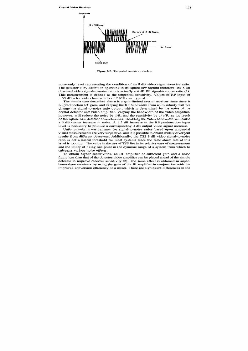
8/8/2019 SciTech - Microwave Passive Direction Finding
http://slidepdf.com/reader/full/scitech-microwave-passive-direction-finding 187/323
Figure 7-2. Tangential sensitivity display.
noise-only level representing the condition of an 8 dB video signal-to-noise ratio.The detector is by definition operating in its square-law region; therefore, the 8 dBobserved video signal-to-noise ratio is actually a 4 dB RF signal-to-noise ratio (1).This measurement is defined as the tangential sensitivity. Values of RF input of- 5 0 dBm for video bandwidths of 2 MHz are typical.
The simple case described above is a gain-limited crystal receiver since there isno predetection RF gain, and varying the R F bandwidth fromBr to infinity will not
change the signal-to-noise ratio output, which is determined by the noise of thecrystal detector and video amplifier. Varying the bandwidth of the video amplifier,however, will reduce the noise by\IBV and the sensitivity by 1/V#V
a s m e resultof the square-law detector characteristics. Doubling the video bandwidth will causea 3 dB output increase in noise. A 1.5 dB increase in the RF predetection inputlevel is necessary to produce a corresponding 3 dB output video signal increase.
Unfortunately, measurements for signal-to-noise ratios based upon tangentialvisual measuremen ts are very subjective, and it is possible to obtain widely d ivergent
results from different observers. Additionally, the TSS 8 dB video signal-to-noiseratio is not a useful threshold for most systems since the false-alarm-rate at thislevel is too high . The value in the use of TSS lies in its relative ease of measurementand the utility of fixing one point in the dynamic range of a system from which tocalculate various noise effects.
To obtain higher sensitivities, an RF amplifier of sufficient gain and a noisefigure less than that of the detector/video amplifier can be placed ahead of the simpledetector to improve receiver sensitivity (2). The same effect is obtained in super-heterodyne receivers by using the gain of the IF amplifier in conjunction with theimproved conversion efficiency of a mixer. There are significant differences in the
Noise only
Time
Bottom of S+N Signal
S+N Signal
Amplitude

8/8/2019 SciTech - Microwave Passive Direction Finding
http://slidepdf.com/reader/full/scitech-microwave-passive-direction-finding 188/323
Pin (dBm)
Figure 7-3. Detector diode—typical characteristics.
two approaches; however: In the RF amplified crystal video system, the detectoris operated in its square-law region; in the superheterodyne, the detector is operatedin its linear region. Figure 7-3 shows the RF-to-video transfer curve of a typicalcrystal detector (3). It may be seen that the square-law range extends from - 4 5
dBm to approximately - 7 dBm, achieving an RF dynamic range of about 35 dB .The detector becomes linear at approximately - 1 0 dBm to about + 40 dBm . Twoother important differences exist: In the RF preamplified crystal video receiver, theRF bandwidthBr is much greater than the video bandwidthBv\ in the superheterodyne,the Br may be only equal to or only slightly greater than twice the video bandwidth(Br = 2BV). These features are desirable for passive direction finding on their ownmerits: The wide RF bandwidth gives maximum probability of detection; the narrowRF bandwidth superheterodyne helps in dense signal environments. All of theseconsiderations make de termination of the expected sensitivity of a receiver difficultto predict unless great care is taken to consider all effects properly.
O
utput
volage

8/8/2019 SciTech - Microwave Passive Direction Finding
http://slidepdf.com/reader/full/scitech-microwave-passive-direction-finding 189/323
7.1.1 Video Detectors
The gain-limited crystal video receiver is defined as such by the fact that the outputsignal-to-noise ratio is due primarily to the noise generated in the crystal detector
and video amplifier input resistance, making the sensitivity dependent on the bandwidthof the video amplifier. This is the condition of insufficient gain ahead of the detectorto establish the output signal-to-noise ratio as a function of a predetection elementsuch as an RF amplifier.
Gain-limited crystal receivers offer the feature of simplicity at the price of lowsensitivity since the equivalent "noise figure" of the simple receiver is poor due toinefficiency of the crystal and problems of matching it to the RF circuit and thevideo amplifier.
Figure 7-4 is a diagrammatic representation of a diode detector in an RF mount,which has an RF input impedance of typically 50 ohms (4). C7 and Rj are the diodejunction capacitance and resistance,Rs andL5 are the ohmic base spreading resistanceand lead inductance;Cp is the parallel capacitance across the holder. The dynamicvideo resistance of the diode is
Ry — R s T Rj
The voltage current equation of the diode is
•• = ' *e x p[ ( iv' )" 1J (7-1}where
i = output currentI5 = the diode saturation current
Figure 7-4. Diode detector equivalent circuit.

8/8/2019 SciTech - Microwave Passive Direction Finding
http://slidepdf.com/reader/full/scitech-microwave-passive-direction-finding 190/323
Vj = the voltage across the diode junction
K = Bo ltzmann's constant
- 1.38 x 10"1 6erg/K
T = the absolute temperature in degrees Kelvin
q = the electrical charge constant (1.6 x 10 "19 C)
The number n is referred to as the "nonideality" factor (5) and may vary from 1to 1.08 for Schottky detectors. The dynamic video resistance of the diode may beobtained by differentiating (7-1) and solving forRj(O, which yields
w = i r i r n ( 7 - 2 )
q(ID + / , )
whereIo = a forward bias current usually applied to the diode to improve its RF imped-
ance matchIs = the saturation current of the diode (~ 10~9 A)
The value of Rj varies with signal level, bias, and temperature. The purpose ofthe above calculation is to obtain an equivalent resistance for the specification ofthe total noise in the receiver.
The sources of noise in the simple video detector consist of the following com-ponents:
1. Thermal noise ofRs in bandwidth Bv
NT = 4KTB VRS
where Bv = .35/pulse rise time2. The shot noise of the junction resistanceRj
It may be shown (6) that
N5 = 2KTB v Rj(l + 7 V )\ 1D + iS /
3. The 1//"flicker" noiseThis low-frequency noise is generally ignored since most video amplifiersare bandpass devices with low-frequency cutoff frequencies above the frequencyat which this effect is significant.
4. The noise power contained in a resistance representing the input impedanceRA of the video amplifier

8/8/2019 SciTech - Microwave Passive Direction Finding
http://slidepdf.com/reader/full/scitech-microwave-passive-direction-finding 191/323
NA = 4KTBVRA
Ignoring the flicker noise, the total output noise voltage is
VN2 = 2KTB v 2RS + Rj (l + 7 + 7 ) + 2RA (7-3)
If the noise contributed by the amplifier can be considered negligible whencompared to the diode, then
VN = \jlKTBv 2[R, + Rj (l + / - A y J ] (7-4)
There have been many attempts to define a figure of meritM for a detector,equivalent to noise figure. Reference 7, an important paper on tunnel diode de tectors,defines it as follows:
M = - ^ ( 7 . 5 )
where
Rv = the dynamic resistance of the diode (per above)
KD = the open-circuit voltage sensitivity of the device in millivolts per milliwatt(mV/mW)
For one type of detector, the tunnel diodeKD can range up to values as high as3000, with Ry values at about 300 ohms. This type of detector operates with a lowconversion loss at low signal levels and a high conversion loss at high signal levels.(If a matching attenuator pad is inserted in series with the detector to effect a betterVSW R match, it will add twice its value to all conversion losses, thus disproportionately
reducing performance.)
On the other hand, Lucas, in a classic paper (8), defines a figure of merit,
Ms = B 5 VR (7-6)
where
B s = the short circuit current sensitivity of the detectorR = a load resistance equal to the video resistance

8/8/2019 SciTech - Microwave Passive Direction Finding
http://slidepdf.com/reader/full/scitech-microwave-passive-direction-finding 192/323
This case assumes no noise contribution from the video amplifier, which is oftenreasonable. Using this value ofM5, the tangential sensitivity of a simple crystalreceiver with no preamplification is
ts = ~r V4KTBV (6.31) (/ + t - 1)M8
-W^-where
ts = the input RF signal power required to achieve TSS
Z ?v = the bandw idth of the video amplifier
K = Boltzmann's constant
t = noise temperature ratio of the detector
T = temperature in degrees Kelvin
/ = noise figure of the video amplifier
/ v = effective noise figure of the video amplifier and detector
Solution of this equation yields typical TSS values in the order of - 4 8 dBm usinga low-noise video amplifier with a 2 MHzBv.
From these equations it may be seen that all of the noise of the gain-limitedreceiver is produced by the detector and video amplifier and that its effective noisefigure is quite high. The signal level necessary to overcome this noise will need tobe fairly substantial, placing it well above the noise in the antenna. Any gain inthe antenna, however, will improve the system's overall sensitivity compared toan isotropic radiator by acting as an ideal amplifier. Maximum sensitivity will beachieved when the RF voltage across the detector junction is at a maximum. Thisoccurs when the detector is well matched to the source (50 ohms). To achieve this
match, diode detectors may be biased, or the detector may be transformed by amatching network to the 50 ohm RF line impedance. If operated with zero bias, ahigher VSW R between the detector and the signal source will result, since the diodedynamic impedance increases reducing power transfer. The relationships are verycomplicated, and although attempts have been made to define a figure of merit fora simple diode, the proliferation of diode types has not resulted in agreement of asingle definition for video receivers.
Point-Contact Silicon Diodes. Point-contact silicon detectors, dating from radartechnology, were the first available types. These detectors, which use a metallic

8/8/2019 SciTech - Microwave Passive Direction Finding
http://slidepdf.com/reader/full/scitech-microwave-passive-direction-finding 193/323
"cat whisker" to contact a semiconductor, exhibit video dynamic resistances ofapproximately 20,000 ohms, dropping to 2000 ohms with approximately 200 |xAof forward bias, which also improves the RF match (lower VSWR) (9). In the daysof vacuum tubes, these resistances permitted high-input impedance amplifiers toact as potential measuring voltmeters, effectively allowing a maximum voltagetransfer to be obtained between the detector and the amplifier's relatively high-input impedance. The limiting factor was the maximum video bandwidth whichwas limited due to upper frequency rolloff from distributed and parasitic capacitydeveloping a reactance equaling the tube's high-input impedance thus makingBv
too low for optimum pulse fidelity. The voltage potentiometer technique, however,allowed Bv to be narrowed for extremely good sensitivities, permitting TSS valuesof - 7 0 dBm to be obtained for very narrow basebands starting at D C , and usefulfor CW detection. Transistor circuits, by contrast, are essentially low-impedancedevices, and the maximum voltage m atch obtained above cannot be easily obtained.Additionally, point-contact diode impedance becomes lower as the RF power in-creases. On the positive side, the point-contact diodes have good high-frequencyresponse due to extremely low junction capacitance. With modern semiconductortechnologies, however, this is no longer significant. The flicker noise problem andthe manufacturing unpredictability of the point-contact detector has reduced itspopularity.
Tunnel Diodes. Tunnel or back-diode detectors biased near their peak forwardcurrent provide the highest rise time response and good sensitivity (expressed inmillivolts per milliwatts). Values of 3500 are typical for low-level signals (7).Although tunnel diode detectors start to depart from square-law at about - 2 0 dB m,their improved sensitivity tend to compensate for this by providing approximatelythe same dynamic range. T unnel diode detectors operate with low-video resistance
loads (~ 300 ohms) and at zero bias, since bias increases the video resistance ascompared to point contact detectors. This operating resistance is fairly constantover the dynamic range . The tunnel diode low-video impedance assures wide band-widths for pulse fidelity, accounting for their improved performance in wideBv
applications. They are about equal to other detectors in narrow video bandwidthapplications; how ever, the unbiased tunnel diode offers a 1// corner frequencyconsiderably (about 3 decades) below that of the crystal detector permitting themto be used for DC detection of CW signals, doppler radar, and zero frequency IF
applications. Tunnel diode detectors have another unusual property: When matchedat low levels they are able to withstand high power well since the reflectivity ofthe diode becomes greater with increasing RF input.
The Schottky Diode. The Schottky barrier or hot-carrier diode is another detectorthat is becoming popular due to its fabrication consistency, very high sensitivity,and low-impedance characteristics. This type of device develops its diode actionby the flow of electrons from a semiconductor(n type) or by the flow of holes (ptype) to a metallic deposited conductor. As shown in Figure 7-5, a "depletion layer"is formed in the manufacture of the diode as electrons or holes flow from the
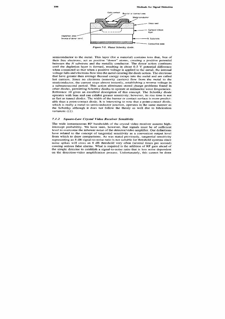
8/8/2019 SciTech - Microwave Passive Direction Finding
http://slidepdf.com/reader/full/scitech-microwave-passive-direction-finding 194/323
semiconductor to the metal. This layer (forn material) contains ions that, free oftheir free electrons, act as positive "donor" atoms, creating a positive potentialbetween the N substrate and the metallic conductor. The donor action continuesuntil the depletion layer is formed, resulting in about 0.5 V potential differencewhen connected so that when a positive voltage is applied to the metal, the internal
voltage falls and electrons flow into the metal creating the diode action. The electronsthat have greater than average thermal energy escape into the metal and are calledhot carriers. Since no electrons (minority carriers) flow from the metal to thesemiconductor, the current stops almost instantly, establishing a reverse voltage ina subnanosecond period. This action eliminates stored charge problems found inother diodes, permitting Schottky diodes to operate at millimeter wave frequencies.Reference 10 gives an excellent description of this concept. The Schottky diodeoperates with bias and can exhibit greater sensitivity; however, its rise time is not
as fast as tunnel diodes. The w idth of the barrier or contact surface is more predict-able than a point-contact diode. It is interesting to note that a point-contact diode,which is really a metal-to-semiconductor junction, operates in the same manner asthe Schottky although it does not follow the theory as well due to fabricationvariances (11).
7.7.2 Square-Law Crystal Video Receiver Sensitivity
The wide instantaneous RF bandwidth of the crystal video receiver assures high-intercept probability. We have seen, however, that signals must be of sufficientlevel to overcom e the inherent noise of the detector/video amplifier. Our definitionshave related to the concept of tangential sensitivity as a convenient output levelfrom which to draw comparisons. As was stated previously, tangential sensitivityrepresenting an 8 dB signal-to-noise ratio is not suitable for threshold systems sincenoise spikes will cross an 8 dB threshold very often (several times per second)causing serious false alarms. What is required is the addition of RF gain ahead ofthe simple detector to establish a signal-to-noise ratio that is less noise dependenton the detection-video amplification process. Unfortunately, this cannot be done
Depletion area(source of donor ions)
Figure 7-5. Planar Schottky diode.
Conductive base
N Substrate
Epitaxial siliconlayer
Glass seal
Metal conductor
Gold contact B a r r i e r o r c o n t a c t a re Q

8/8/2019 SciTech - Microwave Passive Direction Finding
http://slidepdf.com/reader/full/scitech-microwave-passive-direction-finding 195/323
simply for the video signal-to-noise ratios desired due to the square-law action ofthe detector.
Ayer (2) approached the problem of adding gain to a detector by using a broadbandlow-noise traveling wave tube (TWT) amplifier. Starting with the minimum discerniblesignal and with no preamplifier gain, he found that sensitivity increased on a decibel-by-decibel basis as gain was added by the TWT until a maximum sensitivity pointwas reached past which there was no further improvement. From this he developedthe concept of an effective bandw idth,Be. He derived an equation for this bandwidthrelating the RF bandwidthBr and video bandwidth Bv by integrating the noisespectrum across the RF bandwidthBr in one cycle line spectrum intervals. Byperforming this integration after square-law detection and by eliminating terms, theequation for an equivalent bandwidthBe results:
Be = V2B vB r - Bl (7-8)
This equation, which was derived for the minimum discernible signal(S + NIN)0 = 1, considered some of the effects of amplified noise but did not fully coverthe many different signal and noise cross-products conditions encountered over thedynamic range from TSS to gain independence for various ratios ofBv to Bn
Unfortunately, it is not possible to use this concept of an effective bandwidth, exceptfor a very limited case, due to the complicated small signal suppression effectsresulting from complex noise and signal cross products occurring in the RF bandwidth;these effects varying as a function of the signal levels and the ratios ofBr to Bv. Itis important to know how to compute the sensitivity of a RF preamplified crystalvideo receiver, or Ayer's equation may be misapplied, resulting in serious errors.
When sufficient RF gain is applied ahead of a crystal receiver, as shown inFigure 7-6, the receiver will become noise-limited. This is the condition where the
predetection gain is sufficient to ensure that the noise output, in the absence of asignal, is due to detection of the noise figure multiplied by its gain referenced fromthe KTB source noise present in the amplifier's input and source impedance. Sincethe noise figure of microwave RF amplifiers is invariably lower than the equivalentnoise figure of the simple crystal receiver, a dramatic sensitivity improvement isto be expected, and indeed the noise-limited receiver is most desired for passiveDF applications for this reason. Figure 7-7 is a typical plot of the improvement tobe expected by the addition of RF preamplification to a crystal video receiver. A
Detector
FQ = Nose figure of RFamplBr = RFBW
G0=RF Gain
Fv = Nose figure ofvdeo amplBv = Vdeo BW
Figure 7-6. Amplified crystal video receiver.
RFampl
Videoampl
SiN1
So

8/8/2019 SciTech - Microwave Passive Direction Finding
http://slidepdf.com/reader/full/scitech-microwave-passive-direction-finding 196/323
Figure 7-7. Effect of adding gain to a simple crystal video receiver.
typical TSS of —45 dBm is shown for the case of no predetection gain. As gainis added, there is a corresponding increase in sensitivity until the receiver is noiselimited, at which point (shown as 45 dB gain case here) no additional gain willeffect a sensitivity improvement. [The amplifier is shown idealized (noise figure =
1); practical noise figures will reduce the sensitivity as shown.] Correspondingly,decreasing video bandwidthsBv (for a fixed RF bandwidthBr) will increase thesensitivity. It is important to note that the addition of gain decreases the dynamicrange of the system at the expense of using up the square-law region of the detector.There is seldom any virtue in utilizing any more gain than is necessary since it isalso expensive. The transition from the gain-limited receiver to the noise-limitedreceiver is approximately the point after which Ayer's Equation (7-8) can be used(when Br > Bv), as will be shown. There are, however, several problems with this
approach over and above the obvious requirements of gain and/or phase matchingfor DF measurement. The action of the square-law detector plays an important partin the determination of the output signal-to-noise ratio of the receiver for a giveninput signal level. The output of a detector for the conditions of noise alone andfor a signal-plus-noise are depicted in Figure 7-8. Assuming that the input noise isGaussian and the gainGAof the RF amplifier is sufficient to attain the noise-limitedcondition, the video output noise-power spectrum will be of a triangular shape asshown in the shaded section of the figure. This spectrum results from the sum ofall of the noise x noise products of the RF amplifier w ith a bandwidthBv occupiedwithin the bandwidthBn The noise output and the integrated power of all of these
TSS (dBm)
(8P
)U
iD
b jew
id
w
D
aid
J
d
Nose limitedcrystal vdeoreceiver
Gan lmitedcrystal vdeoreceiver
Maxmumsensitivity
TSS withnoRFampI

8/8/2019 SciTech - Microwave Passive Direction Finding
http://slidepdf.com/reader/full/scitech-microwave-passive-direction-finding 197/323

8/8/2019 SciTech - Microwave Passive Direction Finding
http://slidepdf.com/reader/full/scitech-microwave-passive-direction-finding 198/323
The most comprehensive paper on sensitivity, written by Lucas, offers equationsbased upon tangential sensitivity assumptions (RF signal-to-noise = 4 dB) for noiseperformance. Unfortunately, the results have been difficult to use. Tsui (16) hasdeveloped a more flexible formulation for the TSS case of a crystal video receiverfor both the gain and noise limited crystal receiver based upon Lucas.
Note: In the work that follows, all sensitivities will use decibels [10 log(ratio)] instead of the direct ratio formats. Noise figures and system losseswill therefore be nega tive. Gains and band widths will be positive, and allsensitivities will assume variation from the noise present in a 1 MHz bandwidth;that is,
the noise in 1 MH z = 10 log KTB = - 1 1 4 dBm/MH z
where
B = 1.0 MH z
T - 2 90 K
K = Boltzmann's constant
An increase in bandwidth (BW) will be computed as a positive value
10 log(BW)
and added. All lowercase values, for example,/, will refer to ratios in times,whereas uppercase values will refer to this ratio in decibels; for example,
F = 10 log / for predetection andF = 20 log / for postdetection due tosquaring by the detector. The logarithm of a square root is
10 log Vx = 5 log x
and the log of a product is
\og(A)(B + Q = log A + \og(B + C), etc.
The tangential sensitivity Equation (7-7) can be written in a more general formby considering the following: The equation expressed the tangential sensitivity ofthe simple crystal receiver in terms of the effective noise figure of the crystal detectorand video amplifier. If an RF amplifier is added, it provides a gain(gr) and a noisefigure (Jf), the gain being sufficient to allowfr to appear on the detector's transfercurve at a point greater than the tangential sensitivity of the simple receiver. Thiswill add the noise contained in the RF amplifier bandwidth, which when detected,
will add n x n and ^ X u noise in the video bandwidthBv. This must be accounted

8/8/2019 SciTech - Microwave Passive Direction Finding
http://slidepdf.com/reader/full/scitech-microwave-passive-direction-finding 199/323
for by adding Ayer's Equation (7-8) to Equation (7-7). Ayer, in the computationof the effective bandwidthBe, considered only the case of the signal power beingequal to the noise, requiring the addition of another term (2.5 times) to account forthe predetection value of the tangential sensitivity as defined.
The total tangential sensitivity equation, expressed in decibels, has been restatedby Tsui (14) as follows:
T5 = - 11 4 + F A + 10 log 6.31flv + 2.5 VB2e + - ^ 1 ) ^7"9)
\v
(#A/A) /
where
Be = \flBvBr - B2V (from Eq. 7-8)
F A = the R F amplifier noise f igure in decibels (dB )
gA = the RF amplifier gain
6.3 1 = the rat io for TS S (10 log 6.3 1 = 8 dB )
Bv = the vide o amplifier ban dw idth
Br = the R F ban dw idth (usually defined by the preamp lifier)and
A = 1 ^ 1 X 1 0 -6
( 7 - 1 0 )
where
K = flicker noise
/ v = the noise figure of the video amplifier
Rv = dynam ic detector video resistance
M = the detector figure of merit, defined in Equation (7-5)This general equation allows determination ofT8 for both the noise and gain-
limited case. The most notable effect when adding an RF preamplifier is related tothe terms under the square root sign. Considering the most useful case ofBr »Bv, then the effective bandwidth term becomes more significant than the secondterm and for the noise-limited case (definingTsn as the noise-limitedTs):
T8n = - 11 4 + F A + 10 1og(6.31£v + 2. 55 ,) (7-11)

8/8/2019 SciTech - Microwave Passive Direction Finding
http://slidepdf.com/reader/full/scitech-microwave-passive-direction-finding 200/323
Be » Bv for most cases since
Br » 2BV
= - 11 4 + F A + 10 log 2.5 Be
T sn = - 11 0 + F A + 10 1o g£e (7-12)
This is a most useful form and can be used to readily determine the noise-limitedtangential sensitivity. The minimum or confining gain defined as the gainG A necessary tojust assure noise-limitation occurs when
B2= ~ ^ -' (gafaf
Solving for this gain in terms ofTs gives
GA = 110 + Tsv - F r - 10 log Be (7-13)
Solving Equations (7-12) and (7-13) simultaneously to obtain the noise-limitedtangential sensitivity Tsg yields
Tsg = Ts - GA (7-14)
In other words, the tangential sensitivity of the simple crystal video receiver isdirectly improved decibel-for-decibel as long as at least the minimum confininggain GA is used. This is not exact, however, since there is still the small signalsuppression effect to consider.
Let us now consider the gain-limited case. This is readily done by rewritingEquation (7-9) withF A = 0 dB (fA = 1) and GA = 1.
Then
7 ^ = - 1 1 4 4- 10 1og(6.31£v + 2.5 VAB~V) (7-15)
or approximately
Tsg = - 1 1 0 + 10 log VAB~V (7-16)
In this case, A must be determined by using the diode parameters from a vendor'sdata sheet or by actual measurement.
The above equations permit the determination of the tangential sensitivity ofboth noise-limited and gain-limited crystal video receivers. The equations do nottake into account losses that may precede the receiver such as are found in preselec-tors, filters, cables, or the potential system isotropic antenna sensitivity gain when

8/8/2019 SciTech - Microwave Passive Direction Finding
http://slidepdf.com/reader/full/scitech-microwave-passive-direction-finding 201/323
using high-gain horns or other types of antennas. Since most crystal video applicationsuse spiral antennas, with nominal 0 dBi gain, it is easy to forget the improvementa high-gain steerable reflector antenna or multichannel array can provide.
The use of tangential sensitivity derives from World War II methods and tech-niques and is popular because it provides a historical method of comparison of thetechnological advancement in detectors as well as a means of comparing contemporarydes igns . More automated production testing methods rely on the presence of detectorDC shift for a CW signal for accurate sensitivity characterization and parameticmeasurement of intrinsic capacitance resistance and inductance for high-frequencyperformance. In most receiver applications, output signal-to-noise ratio sets thesystem performance. Values of about 15 dB or more are usually required for properthreshold crossing detection w ith typical false alarms of about 1 per minu te. Forthese reasons, the use of the figure-of-merit type comparisons at tangential sensitivityalone is becoming limited, although it is convenient to measure.
The next section presents a signal-to-noise technique that permits sensitivitydetermination for a wide range of output signal-to-noise ratios , and since the tangen-tial signal-to-noise ratio is a convenient defined point, it will be used to compareresults. In practical situations, tangential sensitivity should be used in conjunctionwith other performance factors such as detector conversion efficiency, dynamic
range, RF impedance, match, bandwidth, and operating input and output impedancesto specify total system performance. The equations and methods presented herefacilitate this.
7.1.3 Signal-to-Noise Sensitivity Methods
The preamplified crystal video receiver is relatively easily analyzed for the tangentialoutput signal-to-noise ratio. It is far more useful to develop a general signal-to-
noise output-to-input transfer characteristic to account for a wide range of cond itions.Unfortunately, there has been much disagreement about the methods of this calculationresulting from various interpretations of the works of Rice (12), Lucas (8), andKlipper (13), A first published attempt at clarification, published by this author(15), has resulted in much correspondence and evaluation, the results of which arepresented here.
For a noise-limited amplified crystal video receiver shown in Figure 7-6, the noisespectrum is of the type that was shown in Figure 7-8. There is an outside envelope
that reaches a maximum at DC and tapers off in a triangular fashion reaching azero at the limits ofBv. This describes the base-band noise output, assuming thatthe video amplifier is essentially bandpass filtered. Depending upon the low-frequencycutoff effects, the actual noise output is the result of adding the two noise x noisetriangular areas and the one rectangular area shown in the figure. In the absenceof a signal, there is a constant noise triangular area extending from DC toBv. Thecalculated value of the area bounded by the outer limit to the area defined by thenoise above the triangle gives the output video signal-to-noise ratio. Since thedetector is operating in its square-law region , the various areas are highly dependentupon the amplifier noise figureF and input RF signal-to-noise ratio. For small

8/8/2019 SciTech - Microwave Passive Direction Finding
http://slidepdf.com/reader/full/scitech-microwave-passive-direction-finding 202/323
signal-to-noise input ratios (<1),then X nproducts dominate the output, whereasfor larger signal-to-noise ratios thes x n product is dominant. This relationship istherefore dependent upon the law of the detector, the signal-to-noise ratio, and theratio of the video to RF bandwidth. Because of these dependencies, general rulesare hard to state, and for this reason amplified crystal video receivers have earneda reputation for unpredictable sensitivity calculations. The methods followed herewill attempt to show how more exact computations can be made; however, muchof the theory depends upon assumptions that are not always exact. (An example ofthis is the assumption that all of the noise in the RF bandwidths is Gaussian andthat the shape of the RF bandpass is the same.) Derivation from the tangentialsensitivity case is also somewhat subjective.
Calculation of the noise and signal cross-product areas for the half-wave detectorhas been done by each of the previously cited references and lead in general to anequation that shows the video output signal-to-noise (S/N) ratioX0 as a function ofthe RF input signal-to-noise ratioX1 of the form
X0 = l', Y ( 7 - 1 7 )a + bXj
where a and b are constants defined as follows:
. . ( 2 I H S ; ) 1 fo '" ' <8 '
1 for£v > Br
J 4 ^ . forBv< B rl2b — { B
12 for£v > Brf2
The most useful form of the general equation is forBr » Bv or
(S /N), . W )f2 M I ) - I ; - '
This equation represents the usual case of an RF bandwidth as defined by alossless filter greater than the video bandwidth and has been plotted in Figure 7-9.The video output signal-to-noise ratio is given as a function of the RF input signal-to-noise ratio range for various ratios ofBvIBr..
General Method. To determine the sensitivity of a noise-limited receiver, thebest procedure is to start with the desired output signal-to-noise ratio, determinethe values of Br and Bv, and graphically read the RF input signal-to-noise. To thisvalue add all other losses (such as the loss in the filter that determinesBr) and theeffect of gains due to amplifiers to arrive at the input RF signal-to-noise ratio. This

8/8/2019 SciTech - Microwave Passive Direction Finding
http://slidepdf.com/reader/full/scitech-microwave-passive-direction-finding 203/323
X i = R F signal to noi
Figure 7-9. RF signal-to-noise ratio curves for various

8/8/2019 SciTech - Microwave Passive Direction Finding
http://slidepdf.com/reader/full/scitech-microwave-passive-direction-finding 204/323
procedure is most appropriate since the output signal-to-noise ratio is usually chosento satisfy a required false alarm rate. The following example illustrates the generalmethod using TSS as the desired output signal-to-noise ratio for the purposes ofcomparison. The curves, however, are designed to be used for the full range ofoutput signal-to-noise ratios.
The 8 dB tangential sensitivity line has been drawn as follows:
Bv = 0 . 5 M H z ] 0.5\ BvIBr = Yw = .004
Br = 120MHzJ 1 Z U
F A = 6 d B
GA = 5OdB
Tsr= -44dBm(withnopreamplification)
The desired output tangential sensitivity is 8 dB , which is entered on the abscissaand brought to theBvIBr curve of .004 where an RF input signal-to-noise ratio of- 5 dB is read.
The input signal level to produce an 8 dB signal-to-noise video output level willbe measured below the noise in the RF bandwidthBr. The signal for an 8 dB(signal-to-noise) video output is
(S1) = (available noise in 1 MHz) + F A + (S/N)7 + 10 log Br
= - 1 1 4 + 6 - 5 + 10 log 120
S1 = 92.2 dBm
Let us compare this value to that for the TSS video output case using the equationspreviously derived, recognizing again that we have only used (S/N)o = 8 dB forthis comparison; the method is general for all signal-to-noise values shown on thecurve.
The TSS Method. To proceed, it is necessary to determine if theBe value can
be used directly or if the6.31BV term in Equation (7-11) must be considered; thatis, 6.31BV « 2.5BeforBe:
Be = V2BvBr - Bl = V(2) (.5) (120)
Be = 10.95 X 10⁶ and 2.5Be = 27.3 x 10⁶
Testing this against 6.31BV = 3.15 x 10⁶ shows that Equation (7-11) is preferableto Equation (7-12) since 27 .3 is not > > 3.15.
Substituting in Equation (7-11)

8/8/2019 SciTech - Microwave Passive Direction Finding
http://slidepdf.com/reader/full/scitech-microwave-passive-direction-finding 205/323
Table 7-1. Tabulation of TSS Sensitivities for a Noise-Limited Crystal V ideo ReceiverUsing Three Methods
Hughes Graphically
Initial Amplifier Calculated Determ ined MeasuredBr Bv TSS (db) TSS TSS T SS(M H3) (MH3) (dBm) Gain FA (dBm) (dBm) (dBm)
40 7 .7 - 4 1 51 5 -8 8 . 7 -8 6 . 5 - 8 8120 7.7 - 4 1 48 6 -8 7 .1 84.7 - 8 640 0 .5 - 4 4 53 5 -9 5 . 0 -9 5 . 5 - 9 5
120 0 .5 - 4 4 50 6 -9 3 .0 -9 2 .2 - 9 2
St = - 1 1 4 + 6 + 10 log 30 .5
St = 93.2 dBm
comparing well with 92.2 above.
The gain of 50 dB when added to theTsr of -44 dBm yields -94 dBm, whichis also in reasonable agreement.The results are also in accord with the value of - 9 2 dBm measured and - 9 3
dBm calculated for these conditions (see Hughes, 16).It is interesting to compare other values as calculated by use of the curves to
those calculated and measured by Hughes for various ratios of video and RF bandwidths.Table 7-1 tabulates these results. It may be seen that there is reasonable correspondencefor all methods, with better correspondence whereBr » Bv. In one case, Br —
120, Bv = .5, there was more deviation; however, the amplifier gain was severaldecibels less.The value of the general case is the wide range of values over which the computation
can be made. The value of the tangential calculation method is the ability to predicta point that can be readily measured. It must be remembered that the sufficientconfining gain case is always assumed to be true in the graphical approach.
7 .2 SUPERHETE ROD YNE REC EIVER
The superheterodyne receiver has been in use since the dawn of radio communicationsand certainly before the development of radar. For the particular use in passivedetection D F systems, we are generally interested in two basic forms: the preselectedor "tuned" receiver and the broadband or "downconverted" configurations. This isnot to exclude other designs such as the instantaneous frequency measurem ent,homodyne, or microscan configurations, each of which serves a purpose in theoverall determination of signal presence and identity; however, the specific char-acteristics of the superheterodyne as used for DF purposes m erit particular attention.

8/8/2019 SciTech - Microwave Passive Direction Finding
http://slidepdf.com/reader/full/scitech-microwave-passive-direction-finding 206/323
7.2.1 Sensitivity Determination Methods
Early World War II receivers utilized mechanically scanned RF preselectors trackedto a local oscillator, which could be either a tube or klystron type, to provide a
"window" in the RF spectrum through which signals could enter and be analyzed.RF amplification was not available; therefore, the noise figure of the receiver wassolely dependent upon the preselector loss and the conversion loss of the mixer,which, in turn, depended upon the noise figure of the first intermediate frequencyamplifier. The concept of noise figure(F) was born as a ratio of the noise presentin the actual receiver to that in a theoretically noiseless receiver at a specifictemperature T(K):
_ actual noiseF —noise from ideal receiver atT
F = ^TT (7-19)
where
N0 = actual output noiseNi = KTB noise in the receiver bandwidthB
G = receiver net gain
Modern superheterodyne receivers may contain many active gain stages and mayhave loss elements such as preselectors in series with the mixing and detectionprocess. Consider Figure 7-10, which shows a typical configuration. The overall
noise figure ft is
Figure 7-10. Basic narrow-band superheterodyne.Tuning control
Input
PreselectorRFamp
IFfilter Video output
Famp
Localoscillator

8/8/2019 SciTech - Microwave Passive Direction Finding
http://slidepdf.com/reader/full/scitech-microwave-passive-direction-finding 207/323
, ,* -L (/2 - D , (/3 ~ D , (/4 ~ D ,ft = (Z i + + + + • • •
Sl £l #2 gl£2#3
I Preselector I I R F Amp I I Mixer I I IF AmpI
where each/and g represents the noise and gain ratios.Applying these gain and noise ratios to the computation of overall noise figure,
the preselector exhibits a loss; thereforef\ = Z1. The RF amplifier contribution ishifi ~ 1) since g = III for all values of g < 1. The mixer stage must includethe effects of the IF amplifier or
(/3 ~ D = / i ( /3 ~ D
8182 82
/3 is the mixer loss and may be computed from
/3 = Ic (kfi + t - 1)
where
lc = the mixer convers ion loss
/4 = the IF roof ing filter los s
/5 = the no ise figure of the IF am p
t = nonideali ty factor of the diode (noise temperature rat io)
The equation for the total noise f igure of the receiver can be writ ten as follows:
/ - A + W2 - I) + /, ' K M + ' - ' ) - ! ( 7 . 2 0 )82
assuming that terms past the first IF amplifier can be ignored. From these relationships,the overall noise figure can be calculated.
The concept of confining gain for the superheterodyne relates to supplying sufficientgain in one stage to reduce the noise contribution effects of the next.
As an example, from the equation associated with Figure 7-10
Si
to make the second term negligible so thatft = f\ or that the noise figure of thesuperheterodyne is that of the first stage
8\

8/8/2019 SciTech - Microwave Passive Direction Finding
http://slidepdf.com/reader/full/scitech-microwave-passive-direction-finding 208/323
or gc which is defined as the confining gain which attains our objective.
gc » -^~z—- or approximately
^1
(7-21)gc » ~ — as a good rule
/i
Some logical interpretations of the above equations can be drawn: The noisefigures between passive stages can be added together; for example, the loss of thepreselector adds directly in decibels to the noise figure of the succeeding amplifier(in decibels). The noise figure of the mixer can never be less than the decibel sumof the conversion loss of the mixer and the noise figure of the first IF amplifier.As a practical matter, the noise figure of the mixer is usually the decibel sum ofthe IF amplifier noise figure filter loss and mixer conversion loss, sincet — 2 formost cases. There is also the possibility of oscillator spectrum noise being introducedinto the RF port of the mixer, an important consideration in homodyne or DC IF-type receivers that incorporate IF amplifiers that extend to zero frequency.
The noise figure of wideband RF preamplified superheterodyne receivers mustbe carefully calculated since noise at the image frequency, called the double sideband(DSB ), may be present. The single sideband (SSB) noise figure is generally a moredesired value. Consider Figure 7-11. In Figure 7-1Ia , the noise figure will be thedouble sideband value since in a superheterodyne the mixing action creates twosideband responses from mixing
/ IF=
/L O + /R F
Input PreselectorRFamp
Tunng voltage
a) Doube sdeband noise figure configuration
InputRFamp Preselector
Tunng voltage
b) Snge sdeband noise figure configurationFigure 7-11. (a ) SSB and (b ) DSB configurations for an RF amplified preselected superheterodyne.Receiver (a ) single and (b ) double.
IF
LO
LO
IF
/

8/8/2019 SciTech - Microwave Passive Direction Finding
http://slidepdf.com/reader/full/scitech-microwave-passive-direction-finding 209/323
where
/ I F = the intermediate output frequency
/LO=
the local oscillator frequency/ R F = the input frequency
or
/ R F I=
/LO + /IF
/RF2=
/LO ~ /IF
Either/RPI or/RF2 c a n be used for the signal (the lowest is most often chosen),but if the noise-limited case (sufficient confining gain) prevails, noise will appearat both frequencies. If the IF and preselector bandwidths are purposefully chosento reduce image response, the signal will only appear in one bandwidth, whereasthe noise will be present in both. This contributes a 3 dB increase in the total noise,suppressing the signal. The preselector loss must also be added (in decibels) to the
noise figure of the RF amplifier, degrading the sensitivity even further. The advantageof this arrangement, however, is that only signals present in the narrow preselectorbandwidth are fed to the RF amplifier, thus reducing overload or jamming of theentire band by one or more signals outside the narrow RF frequency band of interest.Figure 7-1 Ib, which places the preselector after the RF amplifier, gives a 3 dBimprovement due to achieving the single sideband noise figure by the eliminationof the image sideband noise and the preselector loss; however, the entire B r of theRF amplifier is exposed to the RF environment.
The ideal solution is the use of a preselector before and after the RF amplifierrequiring that they be tuned or tracked synchronously (tuned to the same frequency).Yittrium iron garret (YIG) voltage tuned filters are commonly used for this purposeand for generation of the variable local oscillator. Tracking can be readily accomplishedwith this arrangement since the YIGs are tuned by a magnetic field generated bya tuning current. This current is quite similar for each YIG assembly, facilitatingtracking. One filter, the preselector, preceeds the RF amplifier, the other, the post-selector, follows the RF amplifier accomplishing the objectives stated above. (The
YIG preselector may also be used for the RF amplified crystal video receiver.)The mixing process of a superheterodyne gives rise to images and a wide variety
of spurious signals. This is due to multiple harmonics of the signal creating mixingproducts that appear at the IF frequency. Care must be taken to assure spuriousfree performance in superheterodyne DF channels since both amplitude and phaseof matched channels can be affected.
The bandwidth of a superheterodyne receiver is usually dictated by the videobandwidth required for maximum fidelity of the received pulse. There are manyconflicting requirements between using the narrowest video bandwidth to optimizedetectability at the expense of pulse fidelity and using the widest bandwidth for
8/8/2019 SciTech - Microwave Passive Direction Finding
http://slidepdf.com/reader/full/scitech-microwave-passive-direction-finding 210/323

8/8/2019 SciTech - Microwave Passive Direction Finding
http://slidepdf.com/reader/full/scitech-microwave-passive-direction-finding 211/323
Figure 7-12. Bandwidth relationships in the superheterodyne receiver.
easily obtained at relatively higher IF frequencies since for a fixed bandwidth it isa smaller percentage of the operating frequency.) The noise figure compromisedirectly reduced the conversion loss of the mixer since the IF noise figure addsdirectly to the mixer. Receivers of this type are called down-conversion superhet-erodyne, implying an IF frequency below the operating frequency.
The sensitivity of this type of receiver must consider three bandwidths: the RFbandwidth, Br, determined by the RF frequency bandpass device and where it isplaced (DSB versus SSB); the IF bandwidth,Bh which is generally made equal toBv\ and the video processing bandwidth.
It is usual practice to assume that the superheterodyne receiver is operating
linearly, permitting the expression of sensitivity to relate to the equation of overallnoise figure F t.The sensitivity of a linear superheterodyne for the case ofB\? = 2BV may be
determined reasonably accurately for output signal-to-noise ratios > > 0 dB byusing the equivalentBe Equation (7-8) in conjunction with the noise figure Equation(7-20) as follows:
Be = V2BrBv - Bv2
where
Br — the smaller of the IF or RF bandwidths
Bv = the video bandwidth
Computing the overall noise figureF t in decibels yields
P r = - 11 4 + F t + 10 log Be + (S/N)o
P
ow
er

8/8/2019 SciTech - Microwave Passive Direction Finding
http://slidepdf.com/reader/full/scitech-microwave-passive-direction-finding 212/323
where
(SfN)0 » O dB
P r = the minimum signal that will provide the desired(SIN)0
This equation is reasonably accurate for the conditions stated above. There are,however, certain cases that limit the above approach: In receivers that have highprocessing gain it may be possible to operate with output signal-to-noise ratios thatare less than 0 dB. There are many applications where the video bandwidth isconsiderably narrower than the RF bandwidth, leading to the equivalent of processinggain (narrow bandwidth CW receivers, for example).
Under these conditions, it is necessary to go back to the methods of determiningthe input (S/N)/ ratio for a desired video output(SIN)0 ratio for the various ratiosof ByIBr as before. To accom plish th is, Figure (7-13) is a curve of a linear detector,plotting the bandwidth ratios parametrically relating (S/N)/ to (S/N)#. By examination,it may be seen that whenBr = 2BV, (BvIBr = .5), the (SIN)0 = (SIN)1 for outputratios greater than zero. For output ratios less than zero and for very narrow bandvideo or, conversely, very wide bandwidth IF or RF conditions, there are majordifferences.
The procedure to follow duplicates that described previously.
1. Determine the required output signal-to-noise ratio.2 . Using the ratioBvIBr, read the input signal-to-noise ratio required at the detector.3 . Compute the input signal powerP 5 at the receiver by using the equation
P 5 = - 11 4 + F t + 10 1o g£r + (SIN)1
This is the signal that will give the required output signal-to-noise ratio for thebandwidths involved.
72.2 Operational Considerations
Superheterodyne dynamic ranges are consistent with the crystal video detectorlogarithmic video amplifier (DLVA) approach since a new log-log video amplifier
is now used. This will be discussed in Chapter 10; however, it is important to notethat modern technology permits the design of a high-quality logarithmic amplifierwith wide bandwidths (greater than 40 MHz typically) and the capabilities ofproviding both RF and demodulated RF to video output for other superheterodyneor crystal video receivers.
Figure 7-14 shows one channel of a typical superheterodyne receiver used by ascanning superheterodyne amplitude monopulse type DF receiver. Two channelswould be required for the monopulse system. The aforementioned dual YIG typeof preselection is utilized for optimum noise and signal performance by scanningthe YIG preselectors with the local oscillator. The receiver is shown with a logarithmic

8/8/2019 SciTech - Microwave Passive Direction Finding
http://slidepdf.com/reader/full/scitech-microwave-passive-direction-finding 213/323
X i = R Fs i g n a lto
Figure 7-13. RF signal-to-noise ratio as functifor a linear detector.

8/8/2019 SciTech - Microwave Passive Direction Finding
http://slidepdf.com/reader/full/scitech-microwave-passive-direction-finding 214/323
Figure 7-14. Single-channel "skirt inhibited" tuned preselector
Ld
Delay line
Andgate
IFamp
Logdet
LocalO S C
IFampI G
RFampI G
RFInput

8/8/2019 SciTech - Microwave Passive Direction Finding
http://slidepdf.com/reader/full/scitech-microwave-passive-direction-finding 215/323
amplifier constructed by placing saturating or logarithmic detectors at each stageand adding the resultant video through an artificial delay-line. A weak signal isamplified by alln stages of the IF; a strong signal saturates the latter stages, whichact as fixed voltage pedestals upon which the earlier stages add their unsaturatedsignals; the delay-line compensates for individual stage delays. The output of thedelay-line therefore is an arithmetic or voltage sum for an input that is geometric.Doubling the RF input, for example, merely adds a voltage (representing a 3 dBinput change) to the output. This may be recognized as the desired logarithmicresponse necessary to achieve wide dynamic ranges and necessary to form themonopulse ratio by subtraction in a multichannel receiver. It is important to notethat measuring the half-voltage video level out of a log system (superheterodyneor DLVA) will not give pulse width. The log action requires that a fixed voltagebe subtracted, as determined by the decibels-per-volt slope of the logarithmic curve.It must also be noted that the bandwidth of a log IF amplifier will change greatlyas a function of signal level since the addition and/or deletion of saturating stageseffectively widens the response in much the same fashion as a limiter, whichincreases the spectrum of the limited signal as its level increases by sharpening therise time. The number of stages in use in a log IF amplifier is determined by theRF input signal, and since the stages contain reactive elements, the number of
bandwidths determining poles will vary accordingly, as each stage saturates.Most superheterodynes scan across a wide bandwidth (typically an octave) andstop when a signal crosses a threshold, set at a level above the noise to ensure anacceptable false alarm rate, the intent being to place the intercept spectrum withinthe passband for analysis and to be able to record the local oscillator frequency touse as an identification word for that signal. It is therefore necessary to be assuredthat the signal is centered within the passband. If the sinxlx pulse spectrum of avery strong pulse crosses the threshold when one of the side lobes is tuned to by
the receiver by the skirts of the IF filter(Br > Z?IF), differentiation of the signalwill occur and the leading edge and trailing edges will appear as "rabbit ears" asshown in Figure 7-15b, a condition where "false triggering" has stopped the localoscillator tuning. The receiver is not centered on the signal properly and may bestopped far from the center RF frequency of the pulse . This effect may be overcom eby a circuit called a skirt-inhibitor. Returning to Figure 7-14, it may be seen thatthe (relatively) linear RF output of the amplifier feeds both a wide and narrowbandwidth skirt inhibitor each tuned to the same IF frequency. If the stopping rules
of the receiver are properly written, stopping will only occur when both are wideand the narrow band filter thresholds are crossed, as shown in Figure 7-15c. Thenarrow bandwidth will distort the pulse; however, the receiver will be properlytuned within the criteria. The wide bandwidth in Figurel-\5d can then be used forsignal measurements, since the signal is fully centered within it and there is nodistortion.
Many different superheterodyne configurations are used. Where YIG or me-chanically tuned preselectors are not desired, image-cancellation m ixers can be usedto prevent stopping at the image frequency or to provide actual cancellation of theimage itself. In other cases, the IF frequency can be chosen to range from DC to

8/8/2019 SciTech - Microwave Passive Direction Finding
http://slidepdf.com/reader/full/scitech-microwave-passive-direction-finding 216/323
Figure 7-15. Action of an IF skirt inhibitor, (a) Real pulse at ^ . (b) Receiver stopped at wrong frequencydue to "rabbit ear" effect, (c) Receiver stopped by narrow band filter at acceptable level, (d) Pulseavailable in wide bandwidth filters channel.
Bv, allowing reception of either the real or the image frequency to stop the receiver.In this case, the resultant frequency resolution (error = 2B V) must not be significant,as is the case for receivers operating at high ( >10 GHz) RF frequencies. Theadvantage here is the improved intercept probability and receiver simplification.
Figure 7-16 shows a homodyne configuration so named for the self-generationof the mixing signal. An oscillator/, at the IF frequency/T F is mixed in a singlesideband modulator (mixer) with one-half of the input signal fs, generating/ L0 =
fs + fo- T h i s output, in turn, is mixed with the other half of/ to generate/ IF since/IF = fo- T n e advantage of the configuration is the potential for wideband, high-
d-Puse avaabe in wde bandwdth filters channe
Threshod
b-Recever stopped at wrong freq due to "rabbit" ear effect
Threshod
a-Rea puse at fp

8/8/2019 SciTech - Microwave Passive Direction Finding
http://slidepdf.com/reader/full/scitech-microwave-passive-direction-finding 217/323
Figure 7-16. Homodyne superheterodyne.
probability detection. The disadvantage is feedthroughof/ LO into the IF (since/LO = / F ) and the requiremen t for high spectural purity of the oscillator since itsDC to "close in" noise adds directly in the mixer, tending to reduce the overallnoise figure.
7 .3 D O W N C O N V E RT E R R E C E I V E R
The advantages of a wide bandwidth crystal video receiver are simplicity, widebandwidth, high frequency-intercept probability, and low cost. The advantages ofthe superheterodyne are high sensitivity, high signal strength detection probability,frequency resolution, and a narrower RF bandwidth that may exclude unwantedsignals. This combines the advantages of better jamming and strong signal environmentimmunity with the disadvantage of reduced instantaneous detection probability.
When an RF amplifier is added to the crystal video receiver, some of the super-heterodyne features are attained; however, there are added problems of dynamicrange and expense.
In the area of warning rece ivers, a new configuration called the baseband receiverhas appeared. This configuration which is essentially a downconverter technique,attempts to attain the best features of both configurations. Figure 7-17 shows themethodology. The usual 2-18 GHz frequency band is multiplex filtered into four4 GHz wide R F segments w ith the purpose of converting each to a 4 GHz basebandin the 2-6 GHz range. The first channel is 2-6 itself and is fed directly to SW3for transfer to the 2-6 GHz baseband system. The 6-10 GHz and the 14-18 GHz
Doublebalancedmixer
Videooutput
Powersplitter
fSRFinput
fS fIF
SSBMixer
IF OSC
fS
fO=fIF
fLO = fS + fO
IFampl

8/8/2019 SciTech - Microwave Passive Direction Finding
http://slidepdf.com/reader/full/scitech-microwave-passive-direction-finding 218/323
Figure 7-17. Down-converter receive
Ra
Ra
Mixer
Mixer
M i x e r
LocalO S C1 6 G H z
LocalO S C1 2 G H z
M u l t i p l e xfilter
14-18GHz
10-14GHz
6 - 1 O G H z
2 - 6 G H z
SW3
SW2W ,

8/8/2019 SciTech - Microwave Passive Direction Finding
http://slidepdf.com/reader/full/scitech-microwave-passive-direction-finding 219/323

8/8/2019 SciTech - Microwave Passive Direction Finding
http://slidepdf.com/reader/full/scitech-microwave-passive-direction-finding 220/323
8. Lu cas, W. J., "Tangential Sensitivity of a Detector Video System with RF Preamp lification,"Proc.IEE VII3, No. 8, Aug. 1966, pp. 1321-1330.
9. Uhlir, A. , Jr. , "Characterization of Crystal Diodes for Low-Lead M icrowave Detectio n,"MicrowaveJournal, July 1963, pp. 59 ff.
10. Adam, S., R. Riley, and P. Szente, "Low-Barrier Schottky Diode Detectors,"Microwave Journal,Feb. 1976, pp. 54 ff.
11. Cowley, A. M., and H. O. Sorensen, "Quantitative Comparison of Solid-State Microwave Detectors,"IEEE Transactions on Microwave Theory and Techniques,MTT-14, No. 12, Dec. 1966.
12. Rice, S., "Mathematical Analysis of Random Noise,"Bell Systems Technical Journal,VoIs. 23and 24, 1945.
13 . Klipper, H ., "Sensitivity of Crystal Video Receivers with RF Preamplification,"Microwave Journal,Vol. 8, Aug. 1965, pp. 85-92.
14. Tsui, J . B. , Microwave Receivers and Related Components,NTK Accession No. PB 84-108711,1983, p. 13, Section 2.3.
15. Lipsky, S. E., "Calculate the Effects of Noise on ECM Receivers,"Microwave, Oct. 1974, pp.65 ff.
16. Hughes, R. S., "Determining Maximum Sensitivity and Optimum Maximum Gain for Detector-Video Amplifiers with RF Preamplification," Naval Weapons Center, Technical Mem orandum 5 357 ,NWC, China Lake, CA, Mar. 1985, p. 14.
17. Konig, C , "ELINT Design Melds Classic M ethods,"Microwaves & RF, Sept. 1984.

8/8/2019 SciTech - Microwave Passive Direction Finding
http://slidepdf.com/reader/full/scitech-microwave-passive-direction-finding 221/323
Probability of Detection
The probability of detecting a signal depends upon many factors in the passive Dreceiver system. There are the obvious necessities of being tuned to the intercepfrequency, to having the intercepting antenna pointing to the intercept, and havinsufficient intercept sensitivity to ensure reception of the target signal down into iback lobes to remove the target scan effectively, if possib le. If the antennas arrotating and sensitivities are limited, a "beam-on-beam" condition, where botantennas must point in each other's direction, may be the only time intercept iaccomplished. If pulses are transmitted, the receiver must be ready when the targis transmitting. Since these conditions prevail for each intercept, it becom es obviou
that the control and setting, or adaptability of the passive DF system, are the majofactors in successful measurement of threat parameters, especially in dense environments.
To ensure proper operation of complex receiving systems, the concept of computecontrol immediately suggests itself and indeed is the method most commonly usedThis idea has been rapidly advanced by the availability of faster and better digitadevices and the obvious acceptance of digital methods in all areas of electronitechnology. It has also been advanced for passive direction finding by the use tha
is made of this information. Since passive DF data derived for threat detection iused for protection, decision making, and control of countermeasure assets, thidea of "power-managed" defensive countermeasures has evolved as the optimumway to direct protective assets to counter priority threats. The electromagnetienvironment signal density has increased to the extent where the decision-makinprocesses in power-managed assets must also be made rapidly. This computer-aideoperator decision-making or semiautomatic operation is becoming the standard. Athe signal density further increases, fully automatic decision making, aided b
artificial intelligence concepts, will undoubtedly prevail.
Chapter Eight

8/8/2019 SciTech - Microwave Passive Direction Finding
http://slidepdf.com/reader/full/scitech-microwave-passive-direction-finding 222/323

8/8/2019 SciTech - Microwave Passive Direction Finding
http://slidepdf.com/reader/full/scitech-microwave-passive-direction-finding 223/323
a limited system that has little memory or a long processing time. Excess computcapacity can be used to average signals, if it is available.
8.1.1 Envelope DetectorTo consider the probability of a burst of noise occurring above a threshold, insteaof a signal, it is necessary to evaluate many conditions relating to the detector. Iit an envelope detector where the video bandwidthBv is optimized for the bestpulse detectability or is it a square-law or linear device? What type of amplifiefollows the detector: linear or logarithmic? Is a signal present with the noise or iit only the noise peak above the noise floor that is triggering the system? As cabe imagined, the analysis of all of these factors is difficult, and since much of ththeory is statistical, most system designers view the results skeptically. The problemrelates to the many variations stated above and the fact that formulation for thestablished radar case does not always apply to the passive DF receiver. To studthe effects of noise, it is necessary to analyze the critical case of noise alone presein a thresholded system.
Consider first the classical radar detection case as stated by Skolnik (1). This ithe case of a superheterodyne radar receiver with sufficient gain to be noise-limite
and with an RF bandwidth determined by the intermediate amplifier bandwidtsuch that
B1. = BIJJ = 2BV
where
Br = BiF is the RF noise bandwidth as determined by the IF bandpass
Bv = the video bandwidth
This type of detector is referred to as an envelope detector. It extracts the shap(envelope) of the modulating signal (pulse) by passing the bandwidthBv of theinformational signal (radar return) while rejecting the RF or IF carrier completelySince this analysis has been used most frequently it will be considered here; how eveenvelope detection is rarely encountered in the passive DF receiver since the widtor bandwidth occupancy of the pulse to be detected is not usually known andBr
is made much greater thanBv by design to improve intercept probability. Figure8-1 is a diagram of the detection model. Noise entering the system is assumed t
RFinput
Detector
y = f(x)
Vdeo amplBv
Comparitoramp
RF amp I"Br
Vt=Threshold voltageFigure 8-1. Detector model for noise-limited false alarm determination.

8/8/2019 SciTech - Microwave Passive Direction Finding
http://slidepdf.com/reader/full/scitech-microwave-passive-direction-finding 224/323
be white and of a Gaussian shape, which means tha t it follows the noise probabilitydensity function
P(v) = J L e x p l - ^
where
a2
= the noise variance
V = the noise voltage
This function is the probability or chance of finding the noise voltage betweenV and V + d(v). The mean value of v is zero. When this Gaussian noise is passedthrough a narrow-band filter and is envelope detected, its characteristics are changedfrom a Gaussian distribution to a Rayleigh distribution of the form
V (- V2\
P(v) = — e xp [ — T ) for V ^ 0
az
\ 2 o - VP(v) = 0 for V ^ 0
This equation is of the form of a Rayleigh distribution. It is possible to plot acurve of the average time between false alarms, defined as TFA, as a function ofth e threshold voltage V t to RMS noise voltage for various values of B v, the videobandwidth. Skolnik defines a term \^ = a
2as the RMS noise power. A similar
curve is drawn in Figure 8-2. For use with the values usually encountered in passiveD F systems, the curve has been expanded and plotted as the log of seconds versusth e threshold-to-noise log voltage to permit greater accuracy. The equation plottedis a plot of
T F A = -1
- exp(V2/ 2a
2) (8-1)
F o r example, in a 10 MHz video bandwidth system for TFA = 100 seconds(log 100 = 2), the F r to- noise threshold should be set to 13.13 dB. As an approxima-t ion PFA, the probability of false alarm for the narrow RF bandwidth case
P F A «l
« EAR№ A
" 2(TFA) (B v) ~ 2B V
( 8 2 )
since
FAR =1
time between false alarms

8/8/2019 SciTech - Microwave Passive Direction Finding
http://slidepdf.com/reader/full/scitech-microwave-passive-direction-finding 225/323
Figure 8-2. Average time between false alarms as ato-noise levels for envelope detection.

8/8/2019 SciTech - Microwave Passive Direction Finding
http://slidepdf.com/reader/full/scitech-microwave-passive-direction-finding 226/323
This approximation assumes that the average duration of a noise pulse is equal tone-half the inverse of the video bandwidth.
8.1.2 False Alarm Probability for Wide RF Bandwidths
Equation (8-1) does not consider the case most often encountered in most warninreceivers; that is, that of a wideband RF,Br » Bv. It also does not address thewideband square-law detector or the use of logarithmic amplifiers ahead of ththreshold process. Several attempts have been made to account for these differenceWhen a wide RF bandwidth of noise is essentially folded into a narrower videbandwidth, a smoothing filter effect takes place. For this reason, it is not easy t
predict the false alarm rate reliably. The matter has been considered by Skolni(1), Harp (2), and Tsui (3). The probability density function of quadratic-detectewideband RF noise, filtered by a narrow-band video filter, is of the form of a chisquare function. For a linear detector, withBr » Bv, the probability densityfunction is assumed to be half-Gaussian. These functions are shown in Figure 8-for each of the three cases. It should be noted that in each case the total area undethe curve is unity(P = 1), the significance of which is that at some level thresholdcrossing will always take place.
To determine a method of analysis for the wide bandwidth, quadratic case, thprobability of false alarm (PFA) for the square-law detector must be calculated fromthe error function (erf) as follows:
PFA = (00P(V)Ci, = 1 - 2 erf (Vv)U? J (8-3)
where
erf = 1 / V 2 ^ [x e~y2/2 dy (8-4)
substituting (8-4) in (8-3) we get
P(V) = - ^ = e x p ( -W 2a2) (8-5)
for V > 0 for the chi-square case.The FAR is related to the PFA as in Equation (8-2). The exact values can be
calculated from error function tables (see Ref. 4) . An easier method is to use Figur8-4, which is a plot of the time between false alarms as a function ofBV9 assumingBr is > 20 Bv. This plot permits determination of the false alarm rate.

8/8/2019 SciTech - Microwave Passive Direction Finding
http://slidepdf.com/reader/full/scitech-microwave-passive-direction-finding 227/323
c) Enveope detector (Skolnik case)Figure 8-3. Probability density function,(a ) Linear detectorBr » Bv. (b) Quadratic detectorBr »Bv. (c) Envelope detector (Skolnik case).
8.2 PROBA BILITY OF SIGNA L DETE CTION IN NO ISE
Up to this point we have determined the false alarm rate of a system by considerinthe possibility of a noise-crossing of a threshold set a certain number of decibelabove RMS noise. We have considered the postdetection case and have related thproblem to the three cases commonly encountered, namely, the envelope-detectoor radar ca se, the wide RF bandwidth wide-open receiver with quadratic-detection
and the intermediate case of a scanning receiver with wide RF bandwidths an
Rayleigh
b) Quadradc detector Br»Bv
Chi-square
a) Linear detector Br»Bv
1/2 Gaussan

8/8/2019 SciTech - Microwave Passive Direction Finding
http://slidepdf.com/reader/full/scitech-microwave-passive-direction-finding 228/323
Xo=Thresholdto noise
Figure 8-4. Average time between false

8/8/2019 SciTech - Microwave Passive Direction Finding
http://slidepdf.com/reader/full/scitech-microwave-passive-direction-finding 229/323
Figure 8-5. Output probability signal densities for Gaussian noise at the output of a linear detector.
video bandwidths not necessarily optimized for the input signal. We must nowdetermine the probability of detecting(P D) a signal in the presence of noise.
When a signal is added to random noise, the presence of both effectively causea shift in the probability density function as compared to noise alone. This is showin Figure 8-5, which is a plot of the log probability density as a function onormalized threshold peak-to-RMS noise for the Gaussian input case for a lineadetector. The predetection curve for noise only, which has a zero mean value(centered about the probability density axis), is translated into a new probabilitdensity function shifted to the right by the addition of the signal. The area of thcurve is a constan t, but the height varies as the RF bandwidth increases with respeto the video bandwidth. When a signal is added, the probability density functio
Peak votage normazed to RMSnose
L
o
g
o
f
p
ro
b
a
b
i
y
d
e
n
s
i
y
Noseonly
»3dbsignaltonoseratio

8/8/2019 SciTech - Microwave Passive Direction Finding
http://slidepdf.com/reader/full/scitech-microwave-passive-direction-finding 230/323
is shifted due to the addition of the noise on top of the signal. The thresholdVt
shown in the figure will be crossed by noise due to the probability density functiowith no signal present. W hen a signal is added and the probability density functiois shifted to the right, the FAR threshold crossings due to noise are represented bthe crosshatched area. Crossings, due to the signal in the presence of noise, in threst of the area to the right of the crosshatched threshold area represent the probabiliof detecting the signal. In passive direction-finding for pulse signals, if a videbandwidth is chosen to be wide for minimum width pulses, wide pulses will furthechange theP D due to a greater look window resulting from the wider pulse and thefact that the pulse will reach its peak value.
The probability of detecting a signal may be the driving factor and will imposa higher threshold requiring a signal level many decibels above the threshold sefor the FAR. To illustrate this, Figures 8-6 to 8-9 have been plotted to provide thprobability of detecting a signal as a function of the signal-to-noise ratio selecte(for whatever the criteria). Although these curves are for a linear detector, themay be used with reasonable accuracy for a square-law detector as well, since thsignal level is high enough to predom inate. The threshold-to-noise ratio is the settinthat may have been established by the FAR or by limitations in the receiver. Thcurves show the actual signal-to-noise ratios that will be necessary for a linea
detector to achieve the probability of detection values(P D) listed.The first curve, Figure 8-6, assumes thatBr is chosen to be wide enough for theminimum expected pulsewidth and that this is the pulse that is received. If, forexample, we had set the threshold above noise by 13.7 dB, we would need aactual 19.75 dB signal-to-noise ratio to achieve 0.90 probability of detection. Wassume that
MIN PW = —By
where Bv is measured at the 3 dB point.It is obvious that if 13.7 dB were chosen for an adequate FAR, the receiver
would have to obtain the higher 19.75 dB value if 0.90 probability of detectiowere to be obtained. It would also be necessary to check to see if 19.75 dB wahigh enough to obtain the required accuracy.
Figures 8-7, 8-8, and 8-9 show that given the choice ofBv, if a pulse two, four,or eight times as wide as the minimum were received, the signal-to-noise requiremenwould drop significantly and could approach the signal-to-noise ratio chosen fothe FAR alone. It is not to be concluded from these curves that the widerBv ismade, the better, since wideningBv will increase the noise FAR, necessitating newthresholding. Computer programmed variable thresholds are often used to achievconstant FAR systems, with programming made variable and appropriate to specifithreat types. Since most systems integrate signals, the high signal-to-noise ratiostated here are markedly reduced in practice by integration or the addition oprocessing gain . Reference 5 gives the effect of pulse integration for the radar caseInterestingly, there is an approximately 5 dB improvement in sensitivity for incoheren

8/8/2019 SciTech - Microwave Passive Direction Finding
http://slidepdf.com/reader/full/scitech-microwave-passive-direction-finding 231/323
Xo=Threshold tonose ratio (db)Figure 8-7. Probability of detection versus signal-to-noise ratio of a video amplifier that is two timeswider than required for minimum pulse width.
P
d
=
P
robabi
y of
d
etecto
n
Xo=Threshold to noise ratio (db)
Figure 8-6. Probability of detection versus signal-to-noise ratio for video bandwidth selected for minimupulse width.
P
d
=
P
robabi
y of
d
etecto
n
Min pulse width
2X Min PW

8/8/2019 SciTech - Microwave Passive Direction Finding
http://slidepdf.com/reader/full/scitech-microwave-passive-direction-finding 232/323
Xo=Thresholdtonose ratio (db)
Figure 8-9. Probability of detection versus signal-to-noise ratio of a video amplifier that is eight timeswider than required for minimum pulse width.
8X Min PW
P
d
=
P
ro
ba
b
i
y ofd
e
te
cto
n
Xo=Threshold to noise ratio (db)
Figure 8-8. Probability of detection versus signal-to-noise ratio of a video amplifier that is four timewider than required for minimum pulse width.
4X Min PW
P
d
=
P
rob
ab
i
y
of
d
e
tecto
n

8/8/2019 SciTech - Microwave Passive Direction Finding
http://slidepdf.com/reader/full/scitech-microwave-passive-direction-finding 233/323
(power added) and 10 dB improvement for coherent (voltage added) pulses foevery decade quantity more pulses used. Curves for the quadratic detector are almoidentical to the linear-detector shown, allowing both cases to use the same valuefrom the curves.
The important point is that a receiver dedicated to receiving a wide range opulsewidths necessitating a largeBv will exhibit a greater detection probability forpulses wider than the minimum width the system was designed to receive. ThwiderBv will increase the FAR, how ever, placing a practical bound upon the systemIntegration is used, in most receivers, typically to reduce the signal-to-noise ratioto familiar values of 8-15 dB for 2-5 degrees accurate DF systems using widbeamwidth (70-90 degree) antennas.
The method of determining the signal-to-noise ratios and the sensitivity of noise-limited square-law detector for a given signal-to-noise ratio is our ultimapurpose. We have seen that this is easily done for the envelope-detector case of narrow RF bandwidth relative to the video bandwidth. It is not as easily done fothe wide RF bandwidth case, however; at this point all the methods necessary havbeen described. To illustrate the technique a step-by-step example will be given
The receiver to be designed as shown in Figure 8-10 has the following characteristic
Bv = 1 MHzBr = 10,000MHzr m i n = 1 microsecond pulsewidth
TFA = 50 seconds (the time between false alarms)
TV = 7 dB (the noise figure of the RF amplifier, which is assumed to have jusenough gain to present the noise limited case and a bandwidthBr)
L = 3 dB (This is the loss of a band-definition preselector ofBr = 10 GHz.It is assumed that theBr of the amplifier is equal to the filter.)
Steps 1-5 determine the sensitivity for a 0.9 probability of detection:Step 1. Find X0 from TFA from the curve shown in Figure 8-4 for the quadratic
detector.Step 2. Log TFA = log 50 = 1.7, readX0 for Bv = 1 from curveX0 = 15 dB .Step 3. Determine the ratioBVIBR:
Preselector
Np detectorTFA
Bv=IMHz= 7db(Br=IOGHz)
L = 3dbBr=IOGHz
Figure 8-10. Model for a wide RF bandwidth(Br) narrow video bandwidth(Bv) quadratic detectorreceiver.
RFampl
y=ax2
Videoampl
SoN0
NQiSj
Vt

8/8/2019 SciTech - Microwave Passive Direction Finding
http://slidepdf.com/reader/full/scitech-microwave-passive-direction-finding 234/323
By = 1 X IQ 6= 4
BR 10 x 109
Step 4. Use Figure 7-9 to obtain the input signal-to-noise ratio,X1 forX0 = 15 dB, readX1 = - 1 0 dB for the 0.0001 curve.Step 5. Compute the noise power(Np) into the detector from the amplifier
(assuming noise limitingGA > TSs) in decibels and taking the noise contributionof BRI Bv:
Np = - 1 1 4 + 10 log(10,000) + JV
= -114 + 40 + 7
Np = -67 dB
Step 6. Determine the input signal 5/ fromN1 by use of the valueX1 fromstep 4:
S1- = N1 + Xt
= - 6 7 + ( - 1 0 )S1 = - 7 7 dBm
Step 7. Add 3 dB for the preselector loss
Si = -74 dBm
This sensitivity assumes an RC roll-off video amplifier that gives an output videwaveform
V = VpJl - exp -(r / rm i n) ]
where
t = the pulsewidth (pw)
'min = UBv where Bv is the 3 dB video bandwidth
V = video filter output voltage
Vpk = peak voltage of the detected pulse fort = o°
V = 0.632 Vpk for t = T min = 1 microsecond
To determine the actual sensitivity for aP^ of 0.9, it is necessary to determinethe sensitivities for the various v ideo bandwidths that may be selected for the receivas part of the design. The - 7 4 dBm sensitivity was determined for the FAR.
8/8/2019 SciTech - Microwave Passive Direction Finding
http://slidepdf.com/reader/full/scitech-microwave-passive-direction-finding 235/323
Step 8. Use Figure 8-6; going back to step 2, the output signal-to-noise ratio fothe FAR is 15 dB , which intersects a horizontal line drawn from the desired detectioprobability(P D) of 0.9 at the 20.75 dB signal-to-noise ratio curve. This means thathe actual signal input powerS[p for PQ of 0.9 is
Sip = - 7 4 + (20.75 - 15.0)
= -6 8. 25 dBm
for a Bv of
Bv = — - - 7 = 1 MHzpw 1 x 10"6
for this case.If it were necessary to use a video bandwidth twiceBv (2 MHz) Figure 8-7 would
give a correction factor of
17.35 - 15 = 2.35 dB
to the —74 dBm sensitivity for a $ip of -71.65. (In this case, interpolation betweenthe curves is required.) The curves are presented for up to eight timesBv andfor the values of signal-to-noise ratios usually encountered. It is important to notthat the sensitivity is improving for the same intercept asBv is made wider than isneeded for a 1 microsecond pulse . The FAR must be rechecked, how ever, for largdifferences. The procedure is general, how ever, and can be used for other condition
Although the above method seems laborious, it relates all of the factors o
bandwidths, detector law, and desired false-alarm rate. It is important to realizthat wide RF bandwidth systems do not necessarily degrade badly in sensitivity foa given P D. Comparing the use of this method in the previous example shown inSection 8.1.1, in a 10 MHzBv for TFA = 1 0 0 seconds the signal-to-noise ratio isabout 15.85 dB compared to 13.13 calculated previously. Harp (2) in anotheexample compares a narrow bandwidth superheterodyne(Br = 20 MHz) to a widebandwidth IFM receiver(Br = 2000 MHz) for the same conditions of probabilityof detection, FAR, and receiver noise figure characteristics, finding only a 5 dB
improvement in sensitivity for the narrow bandwidth case despite a 100 timeincrease in the wideband receiver.
The example shown here is for a linear video amplifier and a quadratic-detectoassuming sufficient gain for the noise-limited case. Any extra gain will reduce thdynamic range of the detector by moving it into its linear range. At low signalevels, however, superheterodyne detectors often operate in the square-law regionwith poor signal-plus-noise-to-noise ratios. This is important in analog systemusing displays since it is possible to use amplitude versus frequency raster scan oan oscilloscope and pulse integration to detect weak signals in the presence of noisfor this method of detection. For digital DF purposes, however, a thresholded sign

8/8/2019 SciTech - Microwave Passive Direction Finding
http://slidepdf.com/reader/full/scitech-microwave-passive-direction-finding 236/323
is usually required , making single pulse crossings important. The equivalent analysof a linear system can be undertaken by using Figure 8-4, which is the noise-onlplot of the average time between false alarms for a linear and approximately quadratdetector in conjunction with Figure 7-13 for the linear-detector. The signal-to-noisinput/output ratio curves now must be chosen for either linear- or quadratic-detectioas appropriate.
8.2.1 Wide RF Bandw idth FARs Using Log Am plifiers
To account for the use of a logarithmic amplifier following the detection processit is necessary to consider the compression effects. Ref. (6) discusses the case oa Gaussian noise input with square-law detection followed by a logarithmic amplifieThe logarithmic threshold in millivolts is within the log curve and is stated here afollows:
VT = V Omin + K' [3.622 + P m - Pinmin + 10 log ( - lo g (PFA)](8-6)
where
VT ~ log amplifier output threshold in millivolts
K' = ( V0 ^ - V0n JZ(P^ - Pinmin) , (8-7)
which is the voltage output variation of the logarithmic amplifier over the definedpower dynamic range of operation (usually given as the slope of the log curve)
PFA = probability of false alarm = 10~6/fl(TFA)
B = an equivalent effective bandwidthBR V 2 r - r2, where r — BvIBr
For a given signal-to-noise threshold not in the log portion, the compressionfactor K' above can be used to modify the(S/N)o ratio of strong signals in the logamplifier as long as the noise threshold is in the linear portion of the logarithmiccurve. The values ofPinmin and the Pinmax will correspond toN0 and S0 in (8-7) fromwhich VT may be determined assumingK' is given for the amplifier. This techniquepermits determination of the log threshold setting for theBR » Bv case, whileEquation (8-6) is the threshold setting for the envelope-detector case(BR = 2BV).
In the case of logarithmic amplifiers, it must be recognized that in the DLVAthe detector is assumed to be in the square-law region and the dynamic range isoften obtained by a piecewise linear approximation of square-law operation at highsignal levels. In the superheterodyne case, a log intermediate frequency ampli-fier is used with detectors that usually operate in the square-law region for smalsignals and in the linear region for large signals.

8/8/2019 SciTech - Microwave Passive Direction Finding
http://slidepdf.com/reader/full/scitech-microwave-passive-direction-finding 237/323
8.3 INTERC EPT PROBAB ILITY
Intercept probability is a time coincidence phenomenon as compared to detectioor false alarm probability, which depends upon receiver sensitivity, bandwidthgain, and noise characteristics. Consider a rotating antenna, scanning bandwidtsuperheterodyne receiver: The sensitivity of such a combination may be highpermitting reception of more than just the mainlobe of the radar transmitter. In thideal case, the first sidelobes and the backlobe may be received, but the superheerodyne, being a narrowband device, may not have scanned to the frequency othe radar, hence no reception will take place until it does. If the frequency scanninis increased to a high speed such that it is always assured of receiving the intercefrequency wherever the DF receive antenna is pointed to the radar intercept, thethe receiver dwell period may be insufficient to receive enough pulses to do integratioand high single-pulse sensitivities will prevail, making only mainbeam detectiopossible. If both the target and receiver antennas are scanning, it may be possiblto attain a beam-on-beam condition where each antenna points to each other. Thcoincidence will improve detection and, in fact, is almost always required for rotasystems. Maximum detection generally prompts high-speed rotation of the interceantenna. This will result in detection eventually; however, if the rotations are i
the same direction and if the rotation rates are equal, no intercept will occur, thilatter condition being generally a trivial case since it is unlikely that both the radatransmitter and radar receiver antennas will be synchronized. Problems can alsexist at harmonic multiples of the rotational rates.
The case for rotating antenna systems usually depends upon having time tperform integration as a natural trade-off for system cost and complexity. Althougit could be argued that nonrotating systems can essentially remove DF antennintercept probability problems, the argument becomes less convincing as millimet
wave radars debut. High atmospheric absorption at certain millimeter frequencbands and difficulties in obtaining power and receiver sensitivities at these frequencimake the use of mechanically positioned systems desirable since high antenna gaiis more easily obtained with narrow beamwidths. Azimuthal rotation of 360 degreeis not always required, since millimeter radars are usually sector-scanned. Ddetecting systems can use the same sector or raster scan techniques using the conceof beam-steering. It may be concluded from this that while phased array andomniazimuthal techniques suggest themselves, mechanical scanning is still a viab
proposition.Frequency scanning also remains an important technique in interception of target
This is due to high sensitivities and the useful properties of step-scan and look-foprioritization of known frequency ranges. The probability of intercept associatewith this process is similar to that of the DF scan. To this must be added the intercepradar pulse time characteristics, since this is another time probability factor.
The current method of expressing intercept probability is to follow the "windowconcept." This theory, presented by Ref. 7, corrected by Ref. 8, and re-presenteby Self (9), represents a reasonably satisfying mathematical mode; however, al

8/8/2019 SciTech - Microwave Passive Direction Finding
http://slidepdf.com/reader/full/scitech-microwave-passive-direction-finding 238/323
characteristics of the system must be idealized, that is, the antennas must havsquare beamwidths, all receiver bandpasses are ideal, all rates are constant, and son.
This book will present both methods for evaluation by the reader. In the interestof understandability, the classical methods of determining intercept probability fothe antenna beam-on-beam technique and the receive scan intercept probabilty wibe considered, first, followed by a discussion of the window concept for generality
8.3.1 Rotating DF Intercept Probability
Up to this point, for passive direction finding we have assumed that the rada
intercept to be received is either constantly illuminating the receiver or that threceiver is a high-sensitivity m onopulse design capable of making a DF m easuremenon each received pulse throughout the radar's scan as the result of normalizatioor removal of the intercept antenna rotation-rate cancellation. This may be accomplished in a dual-channel ratio circuit, the dual-channel being provided by eitheanother co-boresighted antenna or by an omniazimuthal channel conveniently usefor side- and backlobe inhibition of the receiving antenna. The more general casto be considered here will be that of the problem of detecting ascanning targetradar by a single-channelscanning DF antenna system.
Assume the intercept radar antenna has an antenna beamwidthtyr measured 10dB down from the beam peak and rotates with an antenna scan period oftr. Assumefurther that our passive DF system has an antenna beamwidth M^ and a rotationaperiod of td, which is less thantr. It is also implicity assumed thattr ^ td since ifthey were equal and both antennas rotated in the same direction, it could be arguethat no intercept would ever occur (Ref. 8). The probability of detecting a signain one scan of the radar antenna, assuming we are at the proper frequency, is
td < t r
" > S < s -»
where
tyr = the 10 dB radar main-lobe beamwidth
tr = the radar intercept's scan period
td = the DF antenna scan period
The scan periods can be expressed as a function of rotation rate in seconds-perdegree:

8/8/2019 SciTech - Microwave Passive Direction Finding
http://slidepdf.com/reader/full/scitech-microwave-passive-direction-finding 239/323
60
' ' = Nr
Nr = revolutions per minute (rpm)
The probability of detection forn scans of the antenna is
n
PT = E [(P + (1 - P)P + (1 ~ P)2P + • • • + (1 - / V P ]
i
which is a converging geometric series
P D = 1 - (1 - P ) " (8-10)The probab ility of intercepting the radar signal within a given look timeT (noting
that n is the total look timeT divided by the radar scan time, orn = TU1) is obtainedby substituting Equation (8-9) into Equation (8-10). The inverse ofn (which is trlT) is called a window. Performing the substitution gives
/ ^T, t \Tlt r
Equation (8-10) can be rewritten in the form
P D = i - (i - p-yPynP
Since P will be small in one scan,
P D = 1 - e~nP
since
(1 + P)vp = e (approximately)
P D = 1 - exp -(^rT/360td) (8-12)
From Equation (8-12) it may be seen that the probability of detection in a givelook timeT approaches one astd, the period of the DF receiver antenna, approacheszero, which says that the faster the search antenna rotates the better. This rate islimited practically by mechanical problems (speeds up to 1200 rpm have been usedand by the number of pulses it is required to receive from the radar since it iconceivable that the rotation could be faster than a pulse interval. This requires tha
- ^ ^ (PRl)rN (8-13)

8/8/2019 SciTech - Microwave Passive Direction Finding
http://slidepdf.com/reader/full/scitech-microwave-passive-direction-finding 240/323
where
PRI = 1/PRF of the radar
Af = num ber of pulses required
In general, rotating antennas with 4 degree 3 dB beamwidth are weighted by factor of 1.8 to get an equivalent of a 10 dB beamwidth due to the conclusions oEquation (8-13). The usual technique is to consider the 50% probability case ancompute td based upon the number of pulses desired in Equation (8-13). It will befound that rpms of 1000 are required for single-pulse detection capability makinrotating antennas useful for integrating five or more pulses. For this reason rotar
systems are usually used with CRT or other integrating system s. Ref. 10 detailthe use of rotary DF receivers showing that these systems can be made highlycompetitive where simplicity and cost reduction are essential.
8.3.2 Frequency Scan Probability
The previous section defined the probability-of-intercept of receiving a signal wit
both the receiver and radar antennas rotating and the receiver tuned to the radar'frequency. This probability was defined asPp. In this section, we shall assume abeam-on-beam case where both antennas are pointing toward each other, the radais operating at a constant frequency, and the DF receiver is scanning. In a practicacase, this situation is represented by a fixed-antenna system coupled to a high-sensitivity scanning superheterodyne receiver that has sufficient capability to receivthe effects of the radar's antenna scan. It is also assumed that the radar is constantlilluminating the area by operating in the monopulse or CW tracking mode.
Figure 8-11 is a diagram of the situation. A radar w ith a pulse repetition frequencof fr emits a constant amplitude stream of pulses of widthtw as shown at the topof the figure. The pulses occupy an RF bandwidth (frequency occupancy) ofBRrepresenting the sinxlx spectrum of the radar pulses.
The passive detecting receiver with an effective bandwidthBe scans a sector offrequency B that lies between a lower frequency limitfL and a higher frequencylimit // /. This is shown in the lower frequency versus time plot for the receiverThe receiver is scanning periodically from/L to/// at a scan period ofts.
The probability of detecting a radar pulse in one frequency scanPf8 is
Pfs = Hi + t w )f s (8-14)
where
ti = the interval in which the receiver could pick up a radar pulse of widthtw
fs = the pulse repetition frequency of the radar

8/8/2019 SciTech - Microwave Passive Direction Finding
http://slidepdf.com/reader/full/scitech-microwave-passive-direction-finding 241/323
Figure 8-11. Relationships for a nonscanning antenna (constant illuminating) radar as received by ascanning frequency receiver.
The intervalt{ is
'< = ( S P ) ' * ( 8 - 1 5 )
where
ts = the receiver scan rate
Be = the receiver effective bandwidth
B = the sector of scan between the upper frequency limit/// and the lower limih
Br = radar occupany bandwidth
Br =
Radar bandwidth (occupancy)
t Receiver
t Radar
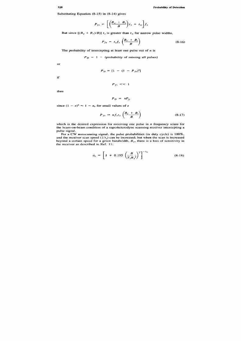
8/8/2019 SciTech - Microwave Passive Direction Finding
http://slidepdf.com/reader/full/scitech-microwave-passive-direction-finding 242/323
Substituting Equation (8-15) in (8-14) gives
But since [(Be + Br)/B)] ts is greater thantw for narrow pulse widths,
(Be + Br\Pfs = t sf s ( B J (8-16)
The probability of intercepting at least one pulse out ofn is
P D — \ — (probability of missing all pulses)
or
P D = [1 - (1 - P fs)n]
if
Pfs « 1
then
PD = «fy
since (1 - e)n
^ 1 - ne for small values ofe
Pfs - »/,*, ( ^ ^ ) (8-17)
which is the desired expression for receiving one pulse inn frequency scans forthe beam-on-beam condition of a superheterodyne scanning receiver intercepting pulse signal.
For a CW nonscanning signal, the pulse probabilities (or duty cycle) is 100%and the receiver scan speed(U ts) can be increased; but when the scan is increasedbeyond a certain speed for a given bandwidth,Be9 there is a loss of sensitivity inthe receiver as described in Ref. 11:
°-- [ '+
° "
5
im )2
}(8
-18)

8/8/2019 SciTech - Microwave Passive Direction Finding
http://slidepdf.com/reader/full/scitech-microwave-passive-direction-finding 243/323
where
a s = the response relative to that obtained with a zero sweep rate
Be = 3 dB receiver bandwidthB = the sweep width or dispersion (in cycles per second)
T1 = the sweep interval in seconds
If R is the resolving power (equalsBe for a s — 1), then the loss in resolvingpower is RIBe\
T = \ (8-19)
where RIB6 is the apparent bandwidth while sweeping relative to the steady-statbandwidth.
In high-scan speed applications, a scanning receiver that can cover a frequencrange during the period of time equal to the pulse width can attain 100% probabiliof scan detection. Receivers of this type are called compressive or microscareceivers. Originally introduced by White and Saffitz (12) and Kinchloe (13), thcompressive receiver holds promise for detection of frequency dispersive signadue to its highP s. Reference (14) is a recent description of this technology.
8.4 WINDOW FUNCTION PROBABILITY CONCEPT
The probability functions we have been considering are actually all idealized; this, we are assuming a square antenna beamwidth rotating over 360 degrees in linear periodic manner, a square receiver bandwidth scanning linearly across frequency range, and so on. These probability-of-detection functions can be analyzein the same manner (com pare the analysis of the DF scan probability to the frequencscan probability above). The method of doing this was discussed by Hatcher iRef. 8. Consider a scanning function to be a time slot periodically appearing at repetitive interval, much in the manner of a pulse train. This is shown in Figur
8-12. Two independent time window func tions,/(A) a n d / (5 ) , represented by pulstrains of widthst\ and t2 and periodsT\ and T2, periodically coincide at which timePi= 1, as shown by the crosshatched areas. It is assumed that the trains are random(not synchronized) nonharmonic, andTx^ T2. These limitations are necessary toprevent the possibility of noncoincidence. It is clear that if one function/(A), foexample, is uncontrolled, as would be the scan of a radar to be intercepted, thethe intercept probability can be increased by optimizing fu nc tio n/ (5 ), which coube the passive DF receiver. This optimization would consist of increasingt2 anddecreasingT2. In a scanning antenna DF receiver, for example, making the antenna

8/8/2019 SciTech - Microwave Passive Direction Finding
http://slidepdf.com/reader/full/scitech-microwave-passive-direction-finding 244/323
Figure 8-12. Intercept probability for two time window functions.
beamwidth greater would increaset2\ increasing the rotational speed of the antennawould decreaseT2.
The probability of intercept can be stated as follows:
For
h ^ T2 - T1
r, = * + •*'- hm>} fo,,«r, (UO)
reducing to
P i = ^ V ^ for r> * * <
8-
2 1>
and for
T2 - Tx =s J1 ^ T2
P 1=I-( 7
' "t 2 )
\ ^T 2
"hf f o r
^ *r
'( 8
"2 2 )
reducing to
Pi= I - {T 2~Th) for T1 ^ t2 (8-23)
2 i i ^ 2
The time Equations (8-20) through (8-23) can represent any scanning functionhowever, care must be exercised not to compute unreasonable conditions of scaspeed, frequency scan as discussed above.

8/8/2019 SciTech - Microwave Passive Direction Finding
http://slidepdf.com/reader/full/scitech-microwave-passive-direction-finding 245/323
8.5 SUMMARY
The probab ility of receiving a signal by consideration of the probability-of-detectioand the probability-of-intercept has been detailed. An important consideration that the probabilities themselves may assume certain conditions. The probability ointercept, for example, assumes the independent conditions that the receiver is tuneto the intercept frequency, a beam-on-beam condition exists, and the signal will breceived. This also assumes that the probability-of-detection criteria are all methat is, the threshold above noise has been set for the proper presence of the signato-noise ratio consistent with the accuracy required and at the proper system falsealarrate.
Probabilities multiply, and as a consequence the total probability-of-detectiomust be computed carefully to be sure that detection takes place within a usefuperiod of time. The scanning antenna, scanning superheterodyne receiver needhigh sensitivity, fast antenna rotation and frequency scan, and wide beamwidthsThese factors may conflict; for exam ple, high-frequency scan speed may desensitithe receiving process; wide antenna beamwidths may reduce DF accuracy; higprobability omniazimuthal, wide-open frequency receiving may offer higher detectiprobabilities but at the expense of higher false-alarm rates and possible ambiguitie
In the world of microwave passive DF, the wide-open instantaneous DF drivereceiver has become standard for threat warning systems where immediacy owarning is important. These systems may be automatic in their detection, recognitioand response since time is of the essence. In electronic intelligence applicationsthe scanning or window probability type systems are useful since they can allowtime for integration or correlation for processing gain to provide high accuracy. Atrade-off is made for use of monopulse techniques on the same basis. Monopulsmethods are useful for pulse-by-pulse warning receivers that are DF and/or frequenc
driven, since monopulse computer sorting provides a relatively fast threat detectiodecision. For collection systems (ELINT), monopulse methods can be used timprove accuracy and calibrate the environment for preparation of a threat scenarithat may be used for the a priori library of the threat warning system.
Our next task will be to study the accuracies that can be expected in varioutypes of systems. These accuracies will reflect back to the method of signal interceptioand will provide a means to determine the signal-to-noise ratios that will provida means to determine the signal-to-noise ratios that will be required on an accurac
basis alone. The passive receiver designer will have to consider all factors anperform a systems performance trade-off for a particular design.
R E F E R E N C E S
1. Skolnik, M. L.,Introduction to Radar Systems,New York: McGraw-Hill, 1962.
2. Harp, J. C , "Receiver Performance, W hat Does Sensitivity Really Mea n?"The International
Counter measure s Handbook, EW Communications, 4th Ed., 1978-1979.3. Tsui, J. B.,Microwave Receivers with Electronic Warfare Application,New York: Wiley, 1986,
Section 2.4, pp. 20 ff.

8/8/2019 SciTech - Microwave Passive Direction Finding
http://slidepdf.com/reader/full/scitech-microwave-passive-direction-finding 246/323
4. Papoulus, A.,Proba bility Random Variables and Stochastic Processes,2nd Ed., New York: McGraw-Hill , 1984, pp. 47-48.
5. Skolnik, M. (Ed.),Radar Handbook, New York: McGraw-Hill, 1970.6. Sakaie, Y ., "Probability of False Alarm and Threshold of Square-Law Detector-Logarithmic Amplifi
for Narrow Band-Limited Gaussian Noise,"IEEE Transactions on Circuits and Systems,Vol. CAS-33, No. 1, Jan. 1986.
7. Hatcher, B. R., "Intercept Probability and Intercept Time,"Electronic Warfare, Mar./Apr. 1976.8. Scheck, P., and A. Behrendt, "Will Intercept Occur." Letters to the Editor,Electronic Warfare,
Mar./Apr. 1977, p. 44.9. Self, G. A., "Intercept Time and Its Prediction,"Journal o f Electronic D efense,Aug. 1983, p. 49.
10. Harper, T., "Are Rotating DF Systems Outdated?"Electronic Warfare, Mar./Apr. 1974, p. 11.11 . Spectrum Analyzer Techniques Handbook,Polarad Electronics Div. of Rohde and Schwartz, Lake
Success, NY, 11042, 1962.12. White, W. D., and I. M. Saffitz, "Compressive Receivers," Topics in Electronics, Vol. 3, 1962,
and U.S. Patent 2,954,465.13. Kinchloe, W. R., "The Measurement of Frequency with Scanning Spectrum Analyzers," Stanford
Electronics Lab, Report 557-2, Oct. 1962, Stanford, CA.14. Tsui, J., "Microwave Receivers and Related Components," National Technical Information Service
Springfield, VA, 1983, PB 84-108711.

8/8/2019 SciTech - Microwave Passive Direction Finding
http://slidepdf.com/reader/full/scitech-microwave-passive-direction-finding 247/323
Accuracy of DF Systems
As we have seen, the probability of detection of a receiving system depends uponfalse-alarm rate, type of receiver technique, the antenna system, and factors establishedby the target such as range, scan, and time modulation factors. Accuracy dependsdirectly on some of these factors; however, we shall study the problem from theviewpoint of how the receiver system designer can optimize the accuracy withrespect to those factors under his control. There is also the question of noise andhow it affects accuracy since it is obvious that noise will mask variations representingsignal changes, degrading accuracy or requiring higher signal-to-noise ratios thatreduce operating sensitivity. The antenna choice and placement, the associated
system balance and dynamic range, and the assignment of the error budget arecrucial conside rations. In any DF system design, there are subtle factors: An aircraftsystem that must fly a great distance along a line of bearing should have a systemthat is very accurate and able to be updated as the target is approached. If thesystem overloads or if the detection process deteriorates as the signal becomesstronger, the m ission will be in vain. In a corollary sense, a warning receiver shouldalways give warning, even if the DF measurement is inaccurate due to receptionof weak signals, since there will be more time available to improve the accuracy,
make decisions, or take action.Much of the accuracy of a system when mounted in an aircraft or on a ship or
other vehicle changes as a function of the environment. The requirement for built-in test facilities (BITE) in most systems tests the operation of the rece iver/processorsubsystems, but rarely the antennas. Various antenna aperture blockages must beconsidered in computing the overall effect of the installation. Illumination of thereceiver by on-board high-power radars may deteriorate one or more channels ofa multichannel receiver, causing a subtle but always present noncatastrophic fault.Periodic calibration and testing must be undertaken to assure that these faults arefound and corrected.
Chapter Nine

8/8/2019 SciTech - Microwave Passive Direction Finding
http://slidepdf.com/reader/full/scitech-microwave-passive-direction-finding 248/323
This chapter will consider the determination of the accuracy of simple andmu ltibeam receiving s ystems of the types described previously. W he re useful, thema the mat ical m od els of the error factors will be prese nted to aid in the deter min ationof an optimum system choice insofar as the system itself determines the selection.
9 .1 A N T E N N A A C C U R A C Y F O R M U L T I B E A M S Y S T E M S
The first discussion of amplitude accuracy will consider the case of DF systemsusually categorized as warning or threat identification types (1). These systems arecharacterized by amplitude comparison of relatively wide-beam antenna patternswith beam widths of approx imately 6 0 - 9 0 degrees. The antennas can be typical lymo un ted at a single point , such as the H one y or a cylindrical array of spira ls, orcan be conformally dispersed about the host vehicle such as is found in aircraftradar warning applications, where antennas may be wingtip or fuselage mounted.The general idea is to provide a complete 360 degree azimuthal field of view thatis distorted as little as possible by the host vehicle. Dispersed antennas such asspirals perform this function w ell, combining w ide R P bandwidth with other desirableattributes such as circular polarization and low cost. For these reasons, this type of
antenna will be considered initially. The equations, however, are fully applicableto narrow multibeam arrays whenever a Gaussian approximation for the patternshapes can be assumed.
9.1.1 The Sine A ntenna Pattern A ssu m ption
The ideal antenna to be used in a four-antenna system would exhibit 90 degree 3dB beamwidths as in Figure 9-1, which shows theE field relationships of a true
sinusoidal 90 degree beamwidth pattern. This type of pattern is achievable byAdc ock an tenna system s and the H on ey antenna , where the pattern shapes arerelatively independent of frequency over a wide bandwidth, typically an octave.
Assuming that the four antennas are suitably deployed and their outputs detectedand logarithmically amplified, it is possible to develop the amplitude monopulseratio for the subtracted log video signals from Chapter 2, Equation (2-9). Takingthe log of the postdetection voltagesVN and VE induced by the presence of the inputsignal arriving at $ we get the monopulse ratioV out :
V0Ut = log VE - log VN = log ^ (9-1 )
and substituting for the field patternswhere
V E = kE
Bsin
§
VN = kN A cos <j)

8/8/2019 SciTech - Microwave Passive Direction Finding
http://slidepdf.com/reader/full/scitech-microwave-passive-direction-finding 249/323
Figure 9-1. Sine field patterns for a four-antenna DF system.
kE and kN = the respective channel transfercharacteristics
V M = l o g ^ (9-2)KN C OS 9
A s s u m i n g B= A
or finally
Vout = log Y tan c() (9 -3 )KN
It may be seen from Equation (9 -3) that any common effects such as scan modulation
or glint (B = A )have been canceled out by the division. This assumes that backlobesof each beam are at a level substantially below the forelobes. This is not alwaystrue (see the H oney antenna discussion in C hapter 3 ), in which case quadrantambiguity will result. The rule for the subtraction requires that the strongest andnext-adjacent strongest antenna be compared, which, when coupled with the backlobeassumption, will assure that the proper pair is being used.
The use of the sine pattern approximation gives rise to the need to balancecarefully the gain of the two channels, represented by the voltageskE and kN in
Equation (9-2). This balance is hard to achieve since the antenna gain of any onelobe varies by only 3 dB over a 45 degree sector, the articulation being only
IncomingSignal

8/8/2019 SciTech - Microwave Passive Direction Finding
http://slidepdf.com/reader/full/scitech-microwave-passive-direction-finding 250/323
6.7 x 10 2 dB per degree. This implies a high degree of match(kE — kN). Toillustrate the match required and the general method of development of the errorequations, consider
where(j)1 = the actual angle of arrival
kE T̂ kN, the general case of mismatch
Let
x = _*LK+\
in general where
Vn = the strongest detected lobe
Vn+I = the next-adjacent strongest detected lobe
^1 = the strongest signal
J cn +1 = the next-adjacent strongest signal
The angular error in degrees is
• " • - • " i i r )
which differs by e, the angular error, such that e =($l - 40 , where $ is thetrue or error-free angle of arrival and tan$ = V n ZV n+ 1
e = tan'1
xt^A -* (9-4)\V
n+\/
Substituting tan § for V JVn+ I gives the error
e = tan"1 (X tan <|>) - c> (9 -5)
To determine the worst case error, Equation (9-5) must be differentiated and set
equal to zero. Using

8/8/2019 SciTech - Microwave Passive Direction Finding
http://slidepdf.com/reader/full/scitech-microwave-passive-direction-finding 251/323
, , , dvldxax a tan v = ^
1 + v2
de _ f X se c2 c|) _ 1
d$ ~ [ I + X2 tan2 c() J
=X s e c 2 c { ) - l - X 2 t a n 2 cj) A
1 + X2 t a n 2 c|)
and set t ing the numerator to zero
X s e c2
c J ) ~ l - Z2
t a n2
cj) = 0
gives
( t an2 <|>) X2 + ( sec2 <)>)X + 1 = 0
Solving for the roots by the quadratic equation gives
-B ± V B2
- 4ACtu ri = 2A
sec2c ( ) ± V s e c4 <(> - 4 t a n2 cj)r i > r 2 _ 2 t an2 C))
But tan2 c() - s ec2 4> — 1.Subst i tu t ing
s e c 2 cf) ± V s e c4 4> - 4 se c2 cj) + 4
2 t a n2 cj)
s e c2 c|) ± (sec2 cj) - 2 )
2 t a n2 cj)
and using the m inus s ign s ince the plus s ign gives the t r iv ia l solut ion, X = I .Substituting and solving for X, then cj) follows
* = 2 = — L -
2 t a n2 cj) tan2 cj)
or
tan cj) = ± — z- (9 -6 )VX

8/8/2019 SciTech - Microwave Passive Direction Finding
http://slidepdf.com/reader/full/scitech-microwave-passive-direction-finding 252/323
and
cf> = t a n "1 ± - * = ( 9 -7 )
V xSolving (9-6) for tan<\> and (9 -7) for c|> in Equ atio n (9 -5) giv es
e = t an"1 (X t an ( (> ) - ( )>
= t a n "1 (X tan cb) - ta n "1 ± — =
V x= t a n "1 X ± —— - t a n "1 ± ——
V x V x= tan"1 ± V X - tan"1 ± ——
V xIn the first quadrant
e = tan"1
V x - tan"1
-^= (9-8)V xwhich permits determination of the error in terms of channel unbalance.
Figure (9-2 ) is a plot of decibel unbalance versus angular error for the sine patterncase of four 9 0 degree beamwidth antennas. A 1 dB unbalance in gain, for ex ample,will cause a 3.2 degree peak error as shown.
9.1 .2 T he Gau ssian A ntenna P attern A ssu m ption
Now consider a different approx imation for the antennas: the use of a G aussian-shaped pattern. Measurements have shown that spiral antennas, in particular, exhibitbeamwidths of this type of the form
P = exp - * ( | r j2 (9-9)
where
c> = the angle of arrival measured from boresight
^ o = one-half the 3 dB antenna beamwidth
K = a constant of proportionality
The radiation pattern of these antennas is shown in Figure 9-3. (Note that in theconfiguration shown, (j), the angle of arrival, is measured from the north boresight.)

8/8/2019 SciTech - Microwave Passive Direction Finding
http://slidepdf.com/reader/full/scitech-microwave-passive-direction-finding 253/323
Figure 9-3. G aussian pattern approx imation for a four-channel am plitude monopulse D F system.
dB unbalance quadratic detector
Figure 9-2. DF error versus channel unbalance for a sine pattern assumption (quadratic detector).
P
e
a
k
e
rro
r
in
d
e
g
re
e
s

8/8/2019 SciTech - Microwave Passive Direction Finding
http://slidepdf.com/reader/full/scitech-microwave-passive-direction-finding 254/323

8/8/2019 SciTech - Microwave Passive Direction Finding
http://slidepdf.com/reader/full/scitech-microwave-passive-direction-finding 255/323
Substituting
v = ^ 0
1/2 = e~k
K = 0.69
replacing k in Equation (9-12), and simplifying gives
* = 6 * " * ( 9 " 1 3 )
Equation (9 -13 ) shows that the angle of arrival ^ measured from the crossoverangle W5/2 is a function of the square of the antenna beam width and is inverselyproportional to squint angle or spacing; it is constant with azimuth. If Equation(9-13) is solved for/?,
_ 6% V
and if R is differentiated with respect to M* to determ ine the e rror s lope, which isdefined as the rate of change of the ratio as a function of the angle of arrival (\Pis directly re lated to 4> by definition above), then
dR 6VSW = ^ f = C ^ c o n s t a n t)
The error slope is determinedonlyby the squint (W5) and the ( 0̂) antenna beamwidthsfor G aussian-form ex pressions of antenna patterns. This means that§ and ^P areonly related to selected constants.If R is measured as the ratio of the strongest tonext adjacent strongest signal, it can yield these angles by comparison to a tableof values independent of the angle of arrival. This is true for all antenna patternsthat can be expressed in exponential form.
The above conclusion permits the use of one look-up table for a DF system
using antennas that exhibit essentially constant beamwidths, such as the spiral, aslong as the pattern can be reasonably ex pressed in the G aussian form. For passivedetection , any G aussian an tenna that is essentially frequency stable in beamwidth,in theory, eliminates the need for a frequency word to correct the DF measurement.This property m akes the broadband spiral useful for radar warning applications overwide frequency ranges (1 0 :1 ). W hen the beamwidths of the spirals do vary (at thelower band edge), band division filters, such as multiplexers as discussed in Chapter4, may be used with associated look-up tables assigned to each band to improve
accuracy due to frequency dispersive beamwidths.

8/8/2019 SciTech - Microwave Passive Direction Finding
http://slidepdf.com/reader/full/scitech-microwave-passive-direction-finding 256/323
Channel Unbalance Accuracy.The unbalance error or difference in gain indecibels between the two operating channels can be determined by calculatingd^ldR from Equation (9 -1 3 ). This is the partial derivative of Equation (9 -1 3 ). It givesthe angle of arrival \P as a function of three variables:R, the log ratio,1P0 the one-half beamwidth, and 5̂ the fixed squint angle:
W2R* = /(J?, ¥ 0 , % ) = - J r (9-14)
Differentiating for e#, the unbalance error, gives
I R ' e¥s ~ €s (9" 15)
The results are plotted in Figure 9-4 for a four-antenna(tys = 90 degrees) DFsystem and in Figure 9-5 for a six-antenna (5̂ = 60 degrees) DF system. Fromthese curves at a given antenna beamwidth Figure 9-6 presents the results for a 1dB unb alance, a common number used in the error budget for systems of this type.The curves can be used two ways: It is possible to determine the amount of error
D
eg
ree
s of
er
or
per
db
unbalance
Antenna 3 ~ d b beamwidth (d eg )
Figure 9-4. DF error (er) as a function of decibel gain unbalance in a four-antenna(Vs = 90 degree)DF system.
Unbalancein db
^ = 9 0°4 Antenna system

8/8/2019 SciTech - Microwave Passive Direction Finding
http://slidepdf.com/reader/full/scitech-microwave-passive-direction-finding 257/323
Antenna beamwidth (degrees)Figure 9-6. Antenna pointing error as a function of antenna beamwidth for a four- and six-antennasystem for a 1 dB unbalance.
D
egrees
of
er
or
per
db
unbalance)
D
egrees of
e
rro
r
per
db
unbala
nce
Antenna 3~db beamwidth (deg)
Figure 9-5. DF error (er) as a function of decibel gain unbalance in a six-antenna (5̂ = 60 degree)DF system.

8/8/2019 SciTech - Microwave Passive Direction Finding
http://slidepdf.com/reader/full/scitech-microwave-passive-direction-finding 258/323
due to unbalance in the channels. For example, in a four-antenna system using 70degree beamwidths, a 1 dB unbalance would cause 2 ,29 degrees of error if the 70degree antenna increased in beamwidth to 100 degrees (at the low-frequency bandend, for ex am ple). The error in degrees for a 1 dB unbalance would equal 4 .6 3degrees, m aking the use of a different look-up table, chosen by a low-band bandpassmultiplex filter, advisab le. The curves assum e a positive 1 dB unbalance using thelower valued channel as reference; if a negative 1 dB unbalance were used, consideringthe upper channel as reference, the error would be negligibly different.
Squint A ccuracy.Variations due to pointing accuracy or squint are important toconsider since squint for broadband antennas will vary with frequency. Also, in the
case of spirals, with the balance of the antenna feed network (balun). Equation(9-13) can be differentiated with respect toW5 to determine e5, the error due tosquint, the actual variation of antenna pointing direction. For planar spiral antennas,this is the angle between a line perpendicular to the plane of the spiral and theactual peak of the beam as it varies from this line.
The error e^ is the partial derivation of Equation (9-14) with respect toWs, or
d¥s~ 6W2
S ~ *s
Substituting R from 9-13 gives
SW W
*¥.--¥. ( M 6 )
The amount of the variation is
€s=~ {v )A*s (9"17)
or the change in the angle of arrival is directly proportional to the change in thesquint angle modified by the ratio of the angle of arrival to the squint angle. F igure
9-7 is a plot of Equation (9-17) showing the degrees of error per squint anglevariation as a function of the angle-of-arrival for different values of squint.
A n te n n a B e a m w id th Va r i a tio nin A c c u r a c y . T h e l a s t e r r o ro f c o n c e r n ,e ^ 0 , i sthe change in DF angle-of-arrivalW with respect to the 3 dB beamw idth variation.This is obtained by taking the derivative ofW with respect to W0
o r again usingEquation (9-13) as follows:
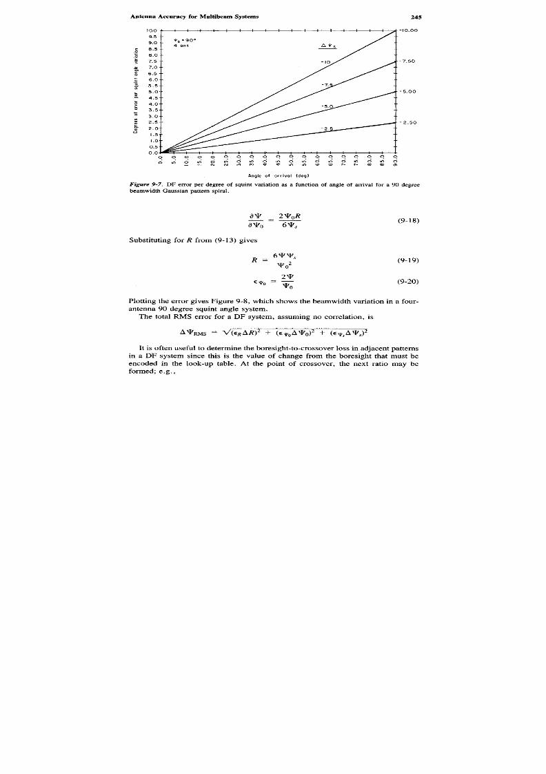
8/8/2019 SciTech - Microwave Passive Direction Finding
http://slidepdf.com/reader/full/scitech-microwave-passive-direction-finding 259/323
Angle of arrivdl (deg)Figure 9-7. DF error per degree of squint variation as a function of angle of arrival for a 90 degreebeamw idth G aussian pattern spiral.
^ - 2 ^ (9-18)
Substituting forR from (9-13) gives
R * * - ^ l <9"
1 9>
«*o = ^ (9-20 )
Plotting the error gives Figure 9-8, which shows the beamwidth variation in a four-antenna 90 degree squint angle system.
The total RMS error for a DF system, assuming no correlation, is
A^RMS = V(€*A/?)2 + (€*0 A % )2 + ( € ^ A ^5 ) 2
It is often useful to determine the boresight-to-crossover loss in adjacent patternsin a DF system since this is the value of change from the boresight that must beencoded in the look-up table. At the point of crossover, the next ratio may beformed; e.g.,
D
e
g
re
es
ofe
rro
r
p
e
r
sq
u
in
t
a
n
g
le
va
ria
to
n

8/8/2019 SciTech - Microwave Passive Direction Finding
http://slidepdf.com/reader/full/scitech-microwave-passive-direction-finding 260/323
A n g l e of a r r i v a l ( d e g )
Figure 9-8. D F error due to variation of 3 dB beam width.
4>=45 (j>=90
R- p ~E J ' R~ rN J4>=0 <|>=45
I t is, however, desirable to control antenna characteristics well into the region ofth e next beam since errors are computed by the straight line logarithmic powerr a t i o . The crossover loss can be determined from Equation (9- 9), or
P(dB)= « P [ - * ( | T )2 ] (9-21)
In decibels,
P(dB) = loiogexp - * M M (9- 22)
Letting r 1equal the ratio
/d>y3 I * / № decibels)
D
e
g
re
e
s
ofe
rro
r
per
3~d
b
b
e
a
m
w
id
th
va
ria
tio
n

8/8/2019 SciTech - Microwave Passive Direction Finding
http://slidepdf.com/reader/full/scitech-microwave-passive-direction-finding 261/323
To check test the case at 45 degrees for a 90 degree beamwidth pattern,
r . = 3 ( j « Y = _ 3 d BV90/2/
which is correct since a 90 degree beamw idth is — 3 dB down from the beam peakat the half power point. For a 45 degree crossover in a four-antenna 90 degreesquinted system, the maximum variation (c|>= ^ 5 = 90 degrees; ^o = 45 degrees)
* - - ( fRx = - 1 2 dB in RF ratio
This means that the total variation from one cardinal axis to another (<() = 90degrees) between two 90 degree beamwidth patternsis 12 dB, which is the decibelpattern variation that shouldbe entered in the look-up conversion tablefor a receiverof this type.
Figure 9-9 is a plot of the crossover sensitivity lossfor a four-beam and six-
beam system for antennas squintedat 90 and 60 degrees, respectively.If the squint
C
r
o
s
s
o
v
e
r
L
o
s
s
(
d
b
)
Antenna Beamwidth (degrees)Figure 9-9. C rossover loss versus antenna beamwidthat the crossover points for four- and six-beamantenna systems.

8/8/2019 SciTech - Microwave Passive Direction Finding
http://slidepdf.com/reader/full/scitech-microwave-passive-direction-finding 262/323
angle is equal to the antenna beamwidth, the maximum mainlobe to crossover losswill always be four times the crossover loss in decibels. If the values differ, theloss must be computed. For example, a typical spiral has a beamwidth of 70 degreesand in a four-channel warning system, the crossover loss is actually
/ 45 \2(^ )4 5 degrees = - 3 l — I = -4 .9 6 dB
and the maximum variation is
/ QQ \ 2(r^ o degrees = ~ 3 ( — 1 = - 1 9 . 8 4 dB
For only a small increase in the 45 degree crossover loss, the articulation of theantenna is improved, relieving the burden of obtaining balance in channels, axialratio balance, and so forth. Fam iliarity with these trade-offs will facilitate assignm entof error budgets and will permit choice of beamwidths and antenna types. A multibeamplanar or circular array can be analyzed using the above procedure assuming G aussianpatterns for the lobes.
9 .2 N O I SE AC C U R AC Y O F AM PL I T U D E C O M PAR I SO N D F SY ST E M S
In C hapter 8, Section 8 .1 , we established that the probability of detecting asignaldepends upon where the voltage threshold is set. W e have established that thethreshold can be set to obtain a given false alarm rate. This may often be theminimum threshold. The operating setting, however, may depend upon a desiredsignal quality, not necessarily the FAR or probability of detecting a signal. Forexample, in a true monopulse analog DF system, it may be required to obtain a0.5 degree resolution using 70 degree beamwidth antennas requiring that an un-ambiguous determinable change be obtained. This would require a signal-to-noiseratio at video of at least
10 log ^ = 21 dB
It is obvious that with no signal integration (the true monopulse case), 21 dB wouldimpose severe sensitivity and dynamic range problems.
If it is assumed that reasonable signal-to-noise ratios will be used, then Equation(9-13) can be used to compute the DF error due to uncorrelated thermal noise asfollows:
* = S ~R (dB) =S "10 (log 5l " log S2) (9"23)

8/8/2019 SciTech - Microwave Passive Direction Finding
http://slidepdf.com/reader/full/scitech-microwave-passive-direction-finding 263/323
Replacing R by 10 (log Si - log S2), where Si and S 2 are signal peak powers,since the powers are proportional to the square of the voltages, gives
2 ( №n
2
OVF 5
where V 1 and V 2 are the signal voltages (after detection).The change in >P with respect to Vi and V 2 can be obtained by taking the partial
derivatives as follows:
E- ** H(i )Figure 9- 10 shows the peak output voltage change for an input noise voltage
{n\fl = A V). This is the approximate case of a small input increment, approximating
the differential (limiting) change. The n\ and n 2 values are RMS noise voltage. It
Figure 9- 10. Relationship between the change in the rear output noise voltage for the two RM S input
voltages AVi and AV2 using the increment A to approximate the derivative.

8/8/2019 SciTech - Microwave Passive Direction Finding
http://slidepdf.com/reader/full/scitech-microwave-passive-direction-finding 264/323
may be seen that since the transfer characteristics of the amplifier (which is logarithmic)is plotted linearly, there is a smaller output noise voltage at a higher input level(V2 is noisier than V1). W e are therefore considering a fairly good signal-to-noiseratio, which would be needed to satisfy the FAR andPD criteria X0 to permit theuse of a G aussian noise distribution. These curves and the calculations are accurateto the degree that this assumption holds. Solving Equations (9-24) and (9-25) for\f in terms of RMS values gives
" • - ^ ^
and
For the RMS A^P1 and A^P2 values, Equations (9-26) and (9-27) must be summedas the square root of the sum of the squares (G aussian assumption):
( A ^ ) R M S = VA ^ 12 + A ^ 2
2 (9-28)
Simplifying and substituting Equations (9-26) and (9-27) into Equation (9-28) yields
But AV2
Il and AV22
/2 can be recognized as the video noise powersN \ and N2,and V2 and V2
2 are the signal powers in channels 1 and 2 used to form the m onopulseratio R. Then, substituting, we get
( A * )m s - i ^ ] l f7 f (9-30,H 's V ^ i ^ 2
Assuming N \ = N2 = N , where A^ and TV2 are uncorrelated noise, gives
R elating the noise error to the ratio of power. ButS2/S \ is the monopulsepowerratio from Equation (9-23) or S2 = g W S V
The equation
/ W s \V 1 . 6 6 ^ 0
2 /

8/8/2019 SciTech - Microwave Passive Direction Finding
http://slidepdf.com/reader/full/scitech-microwave-passive-direction-finding 265/323
can be derived by manipulating Equation (9-23). Finally, the DF error due touncorrelated thermal noise is obtained by substitution
where SNR is the video signal-to-noise ratioThe values for 1P = 45 degrees andW5 = 90 degrees can be substituted for the
four-beam system giving the error A ^ as a function of video signal-to-noise ratioand angle of arrival ^F as
A * = 3 2 .5 V s M(1 + 1 0°2 6 *> (9"
3 3>
which is plotted in Figure 9-11 in two scales and for signal-to-noise ratios of 1 0 -20 dB in the lower curve and 2 5 -3 5 dB in the upper curve.
It is interesting to note that the average error is approximately equal to thatobtained from a rule-of-thumb method. For example, a 20 dB signal-to-noise ratio
Ange ofarrival measured from crossover
Ange of arrivalmeasured from crossoverFigure 9-11. DF error versus angle of arrivalM * measured from crossover for various video signal-to-noise ratios.
E
rro
r
E
rr
o
r
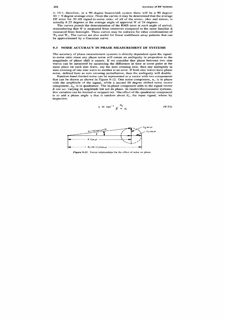
8/8/2019 SciTech - Microwave Passive Direction Finding
http://slidepdf.com/reader/full/scitech-microwave-passive-direction-finding 266/323
is 1 0 :1 ; therefore, in a 90 degree beamwidth system there will be a 90 degree/1 0 - 9 degree average error. From the curves it may be determined that the averageDF error for 20 dB signal-to-noise ratio, of all of the errors, plus and minus, isactually 8.25 degrees at the average angle of approval >P of 24 degrees.
The curves permit the determination of the RMS error ateach angle of arrival,remem bering that Mf is measured from crossover compared to the more familiar ()>measured from boresight. These curves may be redrawn for other combinations of^ 0 and MV The curves are also useful for linear multibeam array patterns that canbe approximated by a Gaussian curve.
9 .3 N O I SE AC C U R AC Y I N PH ASE M E A SU R E M E N T DF SY S T E M S
The accuracy of phase measurement systems is directly dependent upon the signal-to-noise ratio since any phase noise will create an ambiguity in proportion to themagnitude of phase shift it causes. If we consider that phase between two sinewaves can be measured by measuring the difference in time at some point at thesame place on each sine wave, say the zero crossing axis, then any ambiguity inzero crossing of one sine wave to another is an error. If both sine waves have phase
noise, defined here as zero crossing perturbation, then the ambiguity will double.R andom band-limited noise can be represented as a vector with two com ponentsthat can be drawn as shown in Figure 9-12. One noise component,nb is in phasewith the amplitude of the signal, while a second 90 degree shifted noise vectorcomponent, ng, is in quadrature. The in-phase component adds to the signal vectorE cos co?, varying its amplitude but not its phase. In limiter/discriminator systems,this variation can be limited or stripped out. The effect of the quadrature componentis to add a phase angle 7 that is random aboutEr, the input signal, where by
inspection
7 = tan"1 — 5 — (9 -34)E + nt
Figure 9-12. Vector relationships for the effect of noise on phase.

8/8/2019 SciTech - Microwave Passive Direction Finding
http://slidepdf.com/reader/full/scitech-microwave-passive-direction-finding 267/323
F or large signal- to- noise ratios E > n h E > n q,
F s± p t
an d
tan 7 - 7 (approximately)
t h e n
7 ^ 1 (9-35)
T h e total signal power is proportional to the square of E r\
S = E2
nn ~
ni
2"+"
nq
2№ e noise power) (9- 36)
where
nn
2= t h e R M S n o i s e p o w e r
H i2
— p r o p o r t i o n a lto th e / c h a n n e l R M S n o i s e p o w e r
a n d
nq
2= p r o p o r t i o n a lto th e Q c h a n n e l R M S n o i s e p o w e r
S i n c e t h e n o i s e is s ym m e t r i c a l l y d i s t r ib u t e d a b o u tt h e c a r r i e r o >c,
n2
= n2
Since the total noise power
nn
2
= n2
+ n g
2
= 2n q
2
(by substitution)
solving for n q gives
nq
2= "f ( 9 - 3 7 )
As stated above, the only component of the noise creating the phase angle 7 isth e quadrature noise forming the ratio for 7 as follows:

8/8/2019 SciTech - Microwave Passive Direction Finding
http://slidepdf.com/reader/full/scitech-microwave-passive-direction-finding 268/323

8/8/2019 SciTech - Microwave Passive Direction Finding
http://slidepdf.com/reader/full/scitech-microwave-passive-direction-finding 269/323
Figure 9-13. Interferometer phase noise model.
6fl =7
^ s in cj) = - 9 (9 -42 )A
The effects of this noise variation in the m easurement of the angle of arrival <J>of a two-antenna interferometer can be calculated differentiating Equations (9-41)and (9 -42 ) with respect to <|>:
The DF error is
AcJ) = V A c J )/ + A cJ)/ (9-45)
Letting d<\> = AcJ) and substituting from Equations (9-43) and (9-44) gives
AcJ) = nX . V A 9 A
2 + A 6 / (9-46)TTD COS cj)
where A6A = A6# = 7, the phase error in Equation (9-46). Then
AcJ) = — = radians (9-47)iiD cos cj) V S T N
Emitter

8/8/2019 SciTech - Microwave Passive Direction Finding
http://slidepdf.com/reader/full/scitech-microwave-passive-direction-finding 270/323
Angle ofarrival <£
Figure 9-14. Angle error due to noise as a function of angle of arrival for various signal-to-noise ratiosfor dl\ = 0 . 5 .
Figure 9-14 is a plot of the case ofD/X = V i showing the phase error in themonopulse ratio as a function of input signal-to-noise ratio and angle of arrival.The effect of this noise voltage is to fill in the null in a (2 - A ) monopulse systemand to shift the zero crossings or phase differences as a function of1/VS/N . Asmentioned before in the circular phase interferometer, the mode summation improvesthe signal-to-noise ratio in each channel by n, wheren is the multiplier of <j>, theangle-of-arrival. For a given signal-to-noise ratio , the least significant bit will havethe least error and the most significant b it the greatest error, leading to the conclusionthat a combination of amplitude and phase monopulse techniques is desirable; theamplitude monopulse system determines the most significant bit; the phase encoder,the least.
9 .4 A C C U R A C Y AS A FU N C T I O N O F IN S TAL L AT IO N
It is important as part of the general discussion of accuracy of passive DF systemsto consider the location or sighting of the antennas as a fundamental contributor tooverall accuracy. It is unreasonable to expect that antenna pattern measurements
An
g
le
o
f
e
r
o
r

8/8/2019 SciTech - Microwave Passive Direction Finding
http://slidepdf.com/reader/full/scitech-microwave-passive-direction-finding 271/323
made in an anechoic chamber or under ideal conditions will be duplicated in a fieldinstallation. In some instances, the management of the deterioration of DF performanceon the host vehicle can be a major factor in the choice of the appropriate DF system ,more so perhaps, than the expected performance from theoretical considerationsconsidered alone. Configuration of direction-finding systems also depends uponwhether or not the purpose is long-range angle-of-arrival determination or imm ediateDF information for warning purposes and can be further classified on the basis ofintercept probability, angular field of view, response time, and accuracy.
Rotating DF antenna systems make use of more sophisticated receivers sincethere are fewer antennas, thereby reducing the need for multiple channels. Thehigher sensitivity, thus available, may permit reception of side and back lobes of
the signal to be detected, trading receiver cost for complexity. Although a highersensitivity receiver would imply that more signals could be received, the sensitivityusually is the by-product of a narrower RF bandwidth, which as we have seen mayrequire frequency scanning. If time is not a problem, the technique can be used toadvantage to unburden the processing system, since the amount of data madeavailable is limited by the scan.
Fix ed an tennas m ay be located at a single point or geographically dispersed aboutthe host veh icle. In aircraft-mounted radar warning receivers , low gain (0 dBi) wide
band (2 -1 8 G H z) spiral antennas are dispersed about an aircraft effectively enclosingthe vehicle to minimize effects of the unsymmetrical ground plane formed by theaircraft wings, fuselage, and so on. Very high sensitivity is not required in warningapplications, but since 360 degrees of azimuth coverage over a wide-frequencyrange is provided , signal densities can becom e high enough to present serious digitalprocessing difficulties. Direction-finding systems are also greatly dependent uponthe configuration of the ground plane structure around the antennas, reflections fromsurrounding surfaces, and interference from structures or shadowing in the field of
view. The most desirable locations for a fixed-location system, for example, mightbe at the top of a ship's mast or for hemispherical coverage on an aircraft at thelowest point on the fuselage. These locations are rarely available.
Figure 9-15, a plan view diagram of a typical ship, illustrates the type of problemoften encountered in naval installations. It would appear that the top of the mastsystem would be ideal; however, the length-to-width ratio of the ship's groundplane creates pattern distortion and can still cause a problem. Other considerationsare shadowing effects due to other masts, radar antennas, and obstructions.
Reflections can occur due to multipath transmissions in smooth sea states, whichgive rise to inaccurate pulse w idth and DF m easurem ents, both of which can causeprocessing problems unless precision frequency of arrival is also used as a primarysorting tool. One solution to the blockage problem is an antenna system that issectorized into a port and starboard array, which can be mounted on an open faceof the superstructure to provide a clear angle of view. In Figure 9-15, 150 degreesectors of high-accuracy coverage is shown for each side, leaving only two 30degree sectors fore and aft to be covered with lower accuracy 30 degree hornantennas. The sector antennas can be lens-fed arrays or a set of parallel horns.These types of systems offer many advantages:

8/8/2019 SciTech - Microwave Passive Direction Finding
http://slidepdf.com/reader/full/scitech-microwave-passive-direction-finding 272/323
Top view
Figure 9-15. Plan view of a shipborne DF system.
1 . H igh DF accuracy is available port and starboard, w here the ship exhibitsmaximum cross-sectional area to a radar.2 . The reduced DF accuracy fore and aft occurs at minimum ship's radar cross
section.3 . W ith good design it is often possib le to eliminate side- and backlobe inhibition
channels, since the ship's superstructure isolates each wide field-of-viewarray.
In the use of dispersed an tennas, the ground plane effects of the ship are minimized .The dispersed antenna system is generally more expensive; however, since many

8/8/2019 SciTech - Microwave Passive Direction Finding
http://slidepdf.com/reader/full/scitech-microwave-passive-direction-finding 273/323
receiver channels are required, a more accurate and site-independent system canbe configured.
Although sectorized DF systems are perhaps the most accurate, single-point DFsystems work well on smaller ships and are very popular where a true top-of-the-mast location can be found. The A naren fixed B utler-fed circular array in a radom e,as described previously, when mounted on a frigate in the position shown in Figure9-16 (2) was able to attain an R MS accuracy of 1.7 degree R MS in the 8- 1 6 G H zband over a wide variation of angle-of-arrival with respect to the ship. The photographshows what must be considered a nearly ideal location, with minimum apertureblockage, accounting in part for this excellent performance, despite the abovementionedground plane effects.
In aircraft installations , it is desirable to obtain a field-of-view that ex tends aboveand below the horizon to detect the presence of air-to-air and ground-to-air threats(H-plane coverage) as well as provide a 360 degree omniazimuthal DF capability.The use of four or six geographically dispersed spiral antennas is a common solutionfor this requirement. A single point mounted antenna system may also be used forhigh accuracy applications, usually at the price of spatial coverage. Figure 9-17shows a subsonic aircraft outlining antenna location possibilities. Location A showsa belly-mounted radome enclosed rotary antenna. Location B depicts a wing-tip
mount where two or three spirals can be oriented to provide 180 degree coveragefor each side. Locations C and D show how forward and rear quadrants can becovered by mounting two spirals in a radome (location C) and two antennas in thetail structure (location D) for complete 360 degree azimuthal coverage. In thesubsonic aircraft shown, fiberglass radomes are often used to provide protection.
Figure 9-16. Top of m ast location for sea trials of Anaren circular array. C ourtesy of Anaren Microwav eCorp.

8/8/2019 SciTech - Microwave Passive Direction Finding
http://slidepdf.com/reader/full/scitech-microwave-passive-direction-finding 274/323
Figure 9 -17. Typical DF ant
LocationC
ocation B

8/8/2019 SciTech - Microwave Passive Direction Finding
http://slidepdf.com/reader/full/scitech-microwave-passive-direction-finding 275/323
Figure 9-18. An R-KR multiband antenna mounted in a helicopter. C ourtesy of R aytheon C orp.
subsonic aircraft shown, fiberglass radomes are often used to provide protection.In supersonic aircraft, flush-mounted antennas may be dispersed around the aircraft
in a similar manner; however, temperature resistant radomes must be used. Theproximity of aircraft stores such as pods, armament, and other equipment may causeshadowing effects that will definitely affect accuracy. Figure 9-18 shows an R-KRmultiband antenna mounted in a helicopter location that provides 180 degree sectorcoverage . In this cas e, high accuracy is obtained by designing the overall helicopter'sinstallation as a platform for the DF function. Radar warning antennas in helicopterinstallations follow the general rules for subsonic aircraft.
DF accuracy of airborne systems often suffer from antenna depolarization effects,
especially for flush-mounted antennas. Signals that are horizontally polarized seean equipotential surface along the conducting surface skin of the aircraft, whichcancels the horizontal field component leaving only the vertical. Under these conditions,a circularly polarized antenna will tend to exhibit linear or elliptical polarizationalong the fuselage line, causing a null along the aircraft and "grating" or multiple-null lobes. For this reason, it is desirable to disperse spiral antennas at wing andtail tips in a space-quadrature orientation to provide a field of view perpendicularto the plane of the spirals. Perturbations in patterns can be compensated for byanechoic chamber calibrations of aircraft or by site calibrations for ships. C orrectionsof DF measurement as a function of received azimuth or as a function of frequency
RECEVER
DATA PROCESSNG UNT
BAND 3BAND 2

8/8/2019 SciTech - Microwave Passive Direction Finding
http://slidepdf.com/reader/full/scitech-microwave-passive-direction-finding 276/323
can be applied to the DF measurement computation for high-precision or, in thecase of interferometer systems, ambiguity resolution. Digital correction is becominga far more economical solution to improve accuracy than trying to improve theantennas or vehicle mounting locations. This technique is finding favor in thoseinstallations using extensive digital processing where calibration can be accomplished.Other correction methods include the measurement of the elevation angle (6) aswell as the azimuth (<(>) to provide correc tions for aircraft maneuvering .
R E F E R E N C E S
1. Lipsky, E., "U nderstanding DF Accuracy of R adar W arning R eceivers,"Electronic Warfare, DefenseElectronics,Apr. 1978.
2 . "DESM Receiver Sea Trials," Anaren Microwave, Inc., E. Syracuse, NY 13057, 1985.

8/8/2019 SciTech - Microwave Passive Direction Finding
http://slidepdf.com/reader/full/scitech-microwave-passive-direction-finding 277/323
Signal Processingand Display Methods
The various methods and tools of the art of microwave direction finding have been
presented w ith many deta ils. Like all complex designs , there is often a single forcingfunction that governs. In some cases, it is performance; in others, size; in most, itis cost. To be complete, it is also necessary to be familiar with how the outputs ofthe DF system will be used in conjunction with other subsystems. Many of thetechniques, methods, and devices discussed in this book are abstract. This chapterwill examine the methodology of significant hardware aspects of passive directionfinding from a practical viewpoint; that is, the analog processes of detection andamplification over wide dynamic DF range, associated signal processing, and the
popular forms of radar warning and electronic intelligence DF display.
10.1 LOGARITHMICAMPLIFIERS
The logarithmic amplifier finds wide use in passive direction finding systems andcan be a major factor in performance/cost trade-offs. These amplifiers are used toperform two essential functions. The first is the compression of a wide input dynam icrange to a manageable output dynamic rang e; the second is to provide a convenientmathematical method to form the monopulse ratio for normalization. This is doneby subtraction of the logarithmic outputs that form the logarithmic fractional ratio.In passive direction finding, the wide variation of pulse characteristics and the needto cover large instantaneous RF bandwidths have channeled the evolution of thelogarithmic amplifier into specific configurations.
There are four basic types of logarithmic amplifiers: the logarithmic video amplifier,the compressive logarithmic video amplifier, the logarithmic RF amplifier, and thesuccessive detection logarithmic IF amplifier. Each type has certain reasons for usewith DF systems. From an overview, the logarithmic video amplifier is an analog
Chapter Ten

8/8/2019 SciTech - Microwave Passive Direction Finding
http://slidepdf.com/reader/full/scitech-microwave-passive-direction-finding 278/323
amplifier with a logarithmic input/output transfer characteristic designed to complementthe square-law RF-to-video conversion characteristics of a detector. In combinationwith a single detector, this amplifier is known as a detector logarithmic videoamplifier (DLVA) and is characterized by w ide RF and video bandw idth and excellentdynamic range. One variation of this, the second type , is the log -lo g amplifier thatprovides even more dynamic range. Since all phase information contained in thecarrier is lost in the detection process, the DLVA is basically only suitable foranalog/class II processing. The third type, the RF logarithmic amplifier, is an RFconfiguration that operates as a true logarithmic amplifier at the RF or carrierfrequency. Since this amplifier does not detect, all RF phase information can bepreserved permitting use in phase recognition applications analogous to the class I(IAGC) type monopulse processor. The fourth type of amplifier utilizes successivedetection of the RF signal and summation of the resultant video. It develops alogarithmic characteristic from the saturating (or cutoff) gain effects of each of aseries of stages. Since a stage can only contribute a fixed output past a certaindynamic range, an arithmetic sum of these outputs occurs for a geometric inputvariation, resulting in the desired logarithmic response. The successive detectionamplifier finds application as an IF amplifier in most cases and, as described elsewherein this book, is popular for radar and narrow bandwidth scanning receivers. Here
again only amplitude information is preserved.
10.1.1 The Detector Logarithmic Video Am plifier
The most common type of logarithmic amplifier is the detector logarithmic videoamplifier, shown in Figure 10-1. Most DLVAs consist of a wide RF bandwidthdetector preceded by an equally wideband antenna and protective limiter, and sometimesan RF preamplifier. The antenna is usually a spiral, which can cover 2-18 GHz
providing a 16 GH z instantaneous bandw idth. This RF bandwidth can be m ultiplexedinto sub-bands for octave band coverage (2 - 4 , 4 - 8 , 8 -1 6 GH z), as shown inChapter 4, Figure 4-5, in various configurations. The DLVA offers the advantagesof simplicity, wide bandwidth, and relatively good tracking between units. It isideally suited to class II monopulse (subtracted logarithmic amplifier) applicationswhere it can advantageously recover the information bandwidth of the radar videosignal if a sufficiently largeBv is used . The disadvantages are that it is not sensitive,unless preceded by an RF amplifier, and has a somewhat limited dynamic range.This may be overcome by splitting the input signal, adding gain to one channel,and summing both outputs. Another problem of the DLVA may be DC drift. If CWor high duty cycle environments are to be received, DC coupling is desirable. Thehigh gain of the cascaded stages will, however, cause a wide output voltage swingwith temperature by multiplying any small input change by the total DC gain ofthe amplifier, effectively shifting the baseline with respect to a fixed threshold. Aswould be expec ted, this causes changes in the false alarm rate and probability-of-detection of the system. If AC coupling is used, the DC drop across the couplingcapacitor varies with the duty cycle of the environm ent, again shifting the threshold-to-base line settings, creating recovery time problems.

8/8/2019 SciTech - Microwave Passive Direction Finding
http://slidepdf.com/reader/full/scitech-microwave-passive-direction-finding 279/323
Figure 10-1. Detector logarithmi
Logelem
Lo gelement
Logelement
CapacitorwhenA Ccoupled
A
Feedback loopw
Linampl
Limiter/detector
R Finput

8/8/2019 SciTech - Microwave Passive Direction Finding
http://slidepdf.com/reader/full/scitech-microwave-passive-direction-finding 280/323
Figure 10-2. Recovery time problem in an AC coupled logarithmic video amplifier,{a )RF input pulses.(b) Log video output.
To achieve DC stability, many techniques have been attempted. In Figure
10-1, it may be seen that DC loop feedback is possible. Any DC drift can be fedback inversely from the output stage to the input to stabilize the circuit; however,careful attention must be paid to the low-pass filtering since any in-phase high-frequency component existing in the feedback loop will cause oscillation. Since theloop will enclose all ground returns, DC feedback logarithmic amplifiers tend tobe unstable and sensitive to ground loop currents, making layout and shielding asmuch of an art as a science. Successful designs of DC loop amplifiers have beenused for years, however, and this method is useful for moderate video bandwidth
(Bv) devices. Oven stabilization is also used to reduce early stage drift in somedesigns. The other solution, AC coupling, also shown in the figure, is useful aslong as very dense environments or CW signals are not encountered since the DCbuildup across the capacitor will vary with the DC level associated with the firstcomponent of the Fourier series of each pulse train. Also, the DC recovered bydetecting a CW signal is lost unless chopped or otherwise converted to an AC signalthat lies within the video bandpass of the balance of the logarithmic amplifier.
An AC coupled logarithmic amplifier is prone to recovery-time problems. Sincethis is a major consideration, it must be carefully considered at the outset. Figure10-2 details the effect. Assume in Figure 10-2« that four RF pulses are detected
b) Log video output
logvideooutput
a) RF input pulses
RFinput

8/8/2019 SciTech - Microwave Passive Direction Finding
http://slidepdf.com/reader/full/scitech-microwave-passive-direction-finding 281/323
by the receiver. PulseP\ is at approximately —7 dB m , pulseP2 to P4 are at —35dBm or 28 dB lower. The recovered video ofP\ is stretched at low video levelsdue to the shift and duty-cycle DC components of the environment as shown inFigure 10-2&. The result, therefore, is complete masking ofP2 and distortion ofP 3 . It is only after td that P4 can be received and reliably processed. This effectincreases the shadow time of the receiver bytd — t2, where t2 — h is the pulsewidth of the output video andtd is the delay time. It is possible to have delays asgreat as or greater than the pulse width of the strongest pulse, desensitizing thereceiver for extended periods. Solutions for this problem are to increase the ACcoupling by using large capacitors, to DC couple, or to utilize a pulse-on-pulsetype of DLVA, which is described below.
DLVA design starts with the intent to provide a saturating or cutoff plateau atvarious signal levels as determined by the attenuation and logarithmic elements.Hughes describes the design process well in an early paper (1) and in his book (2).Conceptually, each logarithmic video element saturates at a different signal levelas determined by the gain of the linear amplifiers and attenuators. After saturation,the stage holds at a fixed voltage, which is added to the next stage. The unsaturatedgain of each increment follows a logarithmic characteristic due to the input/outputtransfer characteristics of the device.
Figure 10-3 shows two typical logarithmic elements that depend upon theV-Icharacteristics of a diode or diode-connection of a transistor. Temperature drift ofthis type of DLVA depends upon the saturation current variation with temperatureas it passes through the bulk or spreading resistancerb of the diode or transistor.
a) Feedback logarithimiceement usng dode V-I characteristicsDiode
Vout = Log Vin
Vout = Log Vn
b) Feedback ogarithimiceement usng transistor
Figure 10-3. Logarithmic element devices,(a ) Feedback logarithmic element usingV-I characteristics.(b ) Feedback logarithmic element using transistor.
Differentialampl
Differentialampl
Transistor
RoRi
Vin
VinRi
Ro

8/8/2019 SciTech - Microwave Passive Direction Finding
http://slidepdf.com/reader/full/scitech-microwave-passive-direction-finding 282/323
Figure 10-4. Stabilized logarithmic element stage.
Since this current approximately doubles for every 1O0C temperature change, theDC stability for each stage changes, with the earliest stages multiplied by the gainof all successive stages, causing a large output variation. Figure 10-4 permits someimprovem ent by returning the pos itive side of the differential amplifier to the voltagedivider composed byR\ and R^. Reference 3 shows that ifR\ and R2 are chosensuch that
R1 + R1 Ri
the error term is canceled almost completely. The reference also shows a dual
logarithmic amplifier that uses a matched pair differential feedback element toeffectively stabilize both channels, which are then subtracted to form the logarithmicratio in a dual-channel system.
The video logarithmic amplifier must be designed to approximate a straight lineof the plot ofE0 versus RF input to the detector as expressed in dBm . This is shownin Figure 10-5, which is an idealized plot of a compensated amplifier. In this case,more gain is added for high RF inputs (> - 1 0 dBm) to make the output compensatefor the diode detection departure from square law. Points Pi to P3 are the "break
points," where each logarithmic element saturates. P4 is where the stage that isactive for large RF signals (> - 1 0 dBm ) adds its gain, which is purposefully madegreater than the other stages to compensate for the detection law change of thedetector. The compression ratio m, or slope of a logarithmic amplifier, is definedas follows:
output dynamic rangem - . • •••• (in millivolts per decibel)
input dynamic range
Values of 27 mV/dBm are typical.
Differentialampl
Vb-LogVinRo
Ri
«1
Vin
R2
Co

8/8/2019 SciTech - Microwave Passive Direction Finding
http://slidepdf.com/reader/full/scitech-microwave-passive-direction-finding 283/323
In a more recent design approach, Potson and Hughes describe a DC-coupledfast logarithmic amplifier capable of processing 10 nanosecond pu lses. The approachis described in Refs. 4 and 5. An operational amplifier having an inverting andnoninverting input is connected in a current feedback arrangement that forces boththe noninverting and inverting input voltages to be equa l, thus causing the invertinginput impedance to be low. The operational amplifier is designed to have bandwidthrise and fall times independent of the closed loop gain. Figure 10-6 shows theconfiguration. Amplifier A1, which operates over the entire dynamic range, drivesoperational amplifier A2, which has a low input impedance as the result of thecurrent feedback. The gain of Ai is equal to the feedback resistanceRfb divided bythe parallel equivalent res istance due to the parallel combination of the input resistors
Compensation
Detectorsquare-awdeparture
Compnetwork
Det Logampl Log V0F
E0
DBM
RF INPUT
Figure 10-5. Log amplifier output as a function of RF input in dBm into a detector with compensation.
RF

8/8/2019 SciTech - Microwave Passive Direction Finding
http://slidepdf.com/reader/full/scitech-microwave-passive-direction-finding 284/323
Figure 10-6. Current summed series sequential logarithmic amplifier.
Ri, R2, and /?3 and each biased Schottky diode bridgeDi, D2, and Z)3. The diodebridge, which is the nonlinear logarithmic element, is biased and supplied withsignals at various break-point levels as established byRi, R2, and R^ acting asattenuators in conjunction with the dynamic bridge impedances. As the signalincreases, the current to the operational amplifierA2 is sequentially limited, increasingthe parallel input resistance, which inversely reduces the loop gain in a logarithmicmanner. In this way, many break points can be included in a single stage, reducingthe number of stages and the problems associated with DC stabilization. Since thediode bridge is fast, the operational amplifier maintains its bandwidth as the gain
varies, and many break-points can be used. The series-sequential design offers thepossibility for excellent performance for narrow pulses. Since DF technology ismoving up into frequency ranges where 10 -5 0 nanosecond pulse width times maybe expected, this design offers considerable promise for the future. Although DCstabilization may still be needed, the fewer number of stages required simplifiesthis task.
10 J.2 ThePulse-on-Pulse DLVA
The need to reduce the time wasted in the recovery process for strong signals hasprompted development by the AEL Corporation and others of a daily-line "pulse-on-pulse" compressive logarithmic video amplifier. This amplifier, which is a variantof the DLVA, allows only a sam ple of the input pulse width to be amplitude-logged,thus allowing the amplifier to be ready to accept a second pulse immediately afterthe first pulse, even if it occurs during the width or "backporch" of the first. Thetechnique makes use of a reflective delay-line to subtract the pulse from itself thusforcing the amplifier to exhibit base-line gain during the time after a portion of thepulse has been amplified, as shown in Figure 10-7. This permits reception of a
= Schottky diodebridge
Detectedvdeoinput
Driver

8/8/2019 SciTech - Microwave Passive Direction Finding
http://slidepdf.com/reader/full/scitech-microwave-passive-direction-finding 285/323
second pulse before the first has disappeared. Detected positive-going pulses areamplified and fed to a delay-line, which is reactively terminated such that it reflectsthe input pulse, after delaying it bytD and returning it to the input after anotherdelay of tD. By proper choice of constants, the delayed reflected pulse completelycancels all but the portion of the input pulse that was able to pass to node A (twicetD) while the delay-line was being loaded. The output pulse is normalized in widthto 2 x tD as a result.
The logarithmic amplifier consists of DC coupled gain stages A2, A3, and A4.Each stage contains limiting diodes that only conduct at certain positive pulseswings; upon conduction, each diode adds its voltage through theN\ through Af3network, all of which is summed inRL. The noise-limiter is used to suppress
negative-going pulses and noise that are not used in subsequent processing. Additionalcompression can be provided by transistor logarithmic elements in theN networks.This reduces the output dynamic range more than a standard logarithmic amplifier.The curve of output voltage versus power input in dBm is a straight line whenplotted on lo g -lo g graph paper (logarithmic amplifiers use linear-logarithm ic plotsfor straight line outputs). The mathematical effect of this additional compressionis to change the base of the logarithmic system. The pulse-on-pulse technique isfully applicable to the more familiar logarithmic amplifier.
Figure 10-8 shows the result of the pulse-on-pulse design. Two input pulses, Piand P2 , the latter occurring during theP\ interval, are applied to the system. Onlya pulse of a width from the leading edge ofP\ to twice the delay time propagatesthrough the amplifier. The second pulseP2 can therefore be detected and used eventhough it is actually present simultaneously with P1 . This dramatically reduces theshadow time of most systems, which, under ideal conditions, would be at least thewidth of Pi. Contrast this to the pulse recovery time problem shown in Figure 10-2. The output width of the pulses is not equal to that of the original signals, and
pulse width information is therefore lost. DC coupling is applied around the entireamplifier for stability. Detector and the first-stage amplifiers are susceptible to noisepickup; consequently, it is desirable to mount the detector as close to the antennas
Detectedvdeoinput
Deaylineto
Reflectivetermination
Noiselimiter
DCfeedback
Figure 10-7. Pulse-on-pulse logarithmic compression amplifier.

8/8/2019 SciTech - Microwave Passive Direction Finding
http://slidepdf.com/reader/full/scitech-microwave-passive-direction-finding 286/323
Figure 10-8. Pulse-on-pulse logarithmic amplifier operation on two closely spaced pulses,{a ) Pulsefed to delay line, (b) Pulse return from reflective delay line.
as possible. This is also done to reduce RF losses in the connector cable. DLVAunits used in radar warning receivers are therefore often placed in aircraft wingtipsand tail sections, leading to the need for hybrid miniature designs to reduce size.
Log and compressive amplifiers may be built with discrete components or inhybrid form. A hybrid assembly consists of a miniature ceramic printed circuit,which has chip capacitors, resistors, diodes, and semiconductor devices insertedinto mounting holes and bonded to it. This creates a subminiature package that is
a hybrid combination of miniaturized and discrete components, which can be her-metically sealed itself and treated as a subcomponent. Figure 10-9 is a photographof a production version of a hybrid DLVA manufactured by AEL in large quantities.Circuits of this type will undergo further packaging variations as space continuesto be at a premium.
10.1.3 Logarithmic RF Am plifier
Over the years there have been many attempts to develop a true or "detectorless"RF logarithmic amp. This was the intention in the concept of the IAGC systems,
vDetectedvideopulse
a) Pulse fed to delay line
b) Pulse return fromreflective delay line

8/8/2019 SciTech - Microwave Passive Direction Finding
http://slidepdf.com/reader/full/scitech-microwave-passive-direction-finding 287/323
discussed in Chapter 2, but physical settling time, regenerative effects, and un-availability of wideband amplifiers prevented the early development from proceeding.A true logarithmic RF amplifier offers the advantage of preservation of both phaseand amplitude information, permitting many different types of combinationalmonopulse processors to be used. We have seen how both amplitude and phasedetection can be used to resolve ambiguities in many systems and can be used inscanning systems for centering of the tuning local oscillators.
The true logarithmic RF amplifier that has been most successful was designedby Barber and Brown (Ref. 6) and is available as a product from Plessey Semi-conductors. The concept used was to cascade a series of dual-gain stages eachconsisting of an amplifier connected in parallel with a limiter as shown in Figure10-10 Each duo pair consisted of an amplifier that linearly provided gain until thelimiter stage limited, after which the output of the duo pair stayed constant. Thisconstant output was fed to the next cascaded pair and formed a pedestal upon w hichthe next pair built its gain until saturation, and so forth. This is shown in Figure10.10a and b, where each breakpoint indicates where the stage saturation takes
place.Figure 10.10c shows how each duo adds up to form a logarithmic curve with a
slope of
VL
20 log(G + 1)
where
VL = the limiter voltage
Gi = the stage gain
Figure 10-9. Hybrid DLVA. Courtesy o f A EL.

8/8/2019 SciTech - Microwave Passive Direction Finding
http://slidepdf.com/reader/full/scitech-microwave-passive-direction-finding 288/323
Figure 10-10. (a ) Cascade of duo stage pairs consisting of an amplifier and limiter.(b) Resulting gainpiecewise linear approximation, (c) Log characteristics.
Departure fromtrue log response
Log V jn
(dbm)
V jn
vout
b)
c)
AL
Vout
a)
LimiterXl
Voutjn
Linearamp
Breakpoints
G
VL

8/8/2019 SciTech - Microwave Passive Direction Finding
http://slidepdf.com/reader/full/scitech-microwave-passive-direction-finding 289/323
Since there is basically no continuous logarithmic element, as is found in the diodeor transistor case, the error or departure from the logarithmic response curve dependsupon using as little linear gain as possible and therefore requiring many stages,which is not a particularly economical approach. Using hybrid packaging techniques,however, eight-stage true logarithmic amplifiers can be built with an 80 dB RFdynamic range compressed to a 10 V output range useful to 70 M Hz. Phase variation,which was ± 4 degrees in the early model, has been subsequently improved. Reference7 presents an interesting curve that shows single stages versus peak logarithmicerror in decibels for this design . A 12 dB gain stage will give 1 dB of error. Aneight-stage design using 10 dB gain stages should attain a linearity of ± 1 dB . Thetrue RF logarithmic amplifier finds application mainly as a wideband IF amplifierin superheterodyne receivers, since it does not have a wide instantaneous R F bandwidth(Br) as does the DLVA. It also finds use in radar receivers that require phaseinformation moving target indicators, anticlutter, etc.) as well as amplitude data.
10.1.4 Successive Detection Logarithmic Am plifier
The successive detection logarithmic amplifier is, in actuality, a combination of theprevious two designs. It consists of an amplifier chain of a cascade of linear
amplifiers ofn stages that provide maximum RF gain for w eak signals and m inimumgain for strong signals as shown in Figure10-11. This amplifier has been describedpreviously in the study of logarithmic IF systems, where it is most often used. Eachstage of linear gain is detected and clamped to form a pedestal representing themaximum signal at that point. Each pedestal is in turn summed through a delayline to provide a logarithmic video output. The delay line is used to compensatefor stage delay and to reduce recovery time. The RF output is not linear since thedetection process distorts the total dynamic range; however, with careful design
some gross phase information can be obtained.There are several variations of the circuit shown. For IF applications, the stages
may be coupled together by resonant interstage networks, the purpose being to limitthe RF instantaneous bandwidth desirable for superheterodyne image rejection, andso on. In sum and difference applications, this may create a problem since thenumber of poles that determines the RF band pass becomes proportional to thesignal strength. Since the sum channel will be of greater amplitude than the differencechannel in null systems, the phase error due to dynamic range may be significant
since the num ber of poles in use in each channel differs affecting phase . L ogarithmicamplifiers compress the response of filters. Therefore, all filtering should be donewith a multipole sharp slope filter (near ideal).
The successive detection amplifier as shown can be used for bandwidths up tothose frequencies where parasitic effects in the detector diodes become a problem.It is possible to design the system with an iterative impedance of 50 ohms andfollow microwave techniques; however, the DLVA can offer a less costly solution.For these reasons, the successive detection amplifier is used for video and IFapplications in frequency ranges up to approximately 200 MHz. Care must beexercised in layout, however, to prevent instability due to high gain, and so on.

8/8/2019 SciTech - Microwave Passive Direction Finding
http://slidepdf.com/reader/full/scitech-microwave-passive-direction-finding 290/323
Figure 10-11. Successive detectio
Delayline
L inina m p l
Detectors
Limiters
Lina m p l
R o
R F i n

8/8/2019 SciTech - Microwave Passive Direction Finding
http://slidepdf.com/reader/full/scitech-microwave-passive-direction-finding 291/323
Input power (dBm)Figure 10-12. Matching characteristics of two 160 MHz successive detection logarithmic IF amplifiers.Courtesy of the RHG Corp.
There are comm ercial logarithmic R F amplifiers available capable of being m atched
to within ± .5 dB . Figure 10-12 is a plot of the departure from ideal logarithmiccharacteristics for an RHG corporation 160 MHz center frequency design. Theamplifiers have a 30 MHz bandwidth response and exhibit the indicated match overan 80 dB dynamic range (with a slope of 25 mV/dB).
10.2 A PHASE CORRELATOR FOR WIDEBAND APPLICATIONS
The wide RF bandwidth phase correlator is, in a way, analogous to the widebandwidth detector logarithmic amplifier since it provides a means to measuredifferences in phase to a high degree of precision. The first use of the phase correlatorwas to measure the differences in phase resulting from the time delay in one pathof a dual output coupler. The insert in Figure 10-13 shows the idea: Any signalfed to the RF input would arrive as two voltages, where the differences betweenthe angles A and B were proportional to the time delayt established by the delayline. The purpose of the correlator, shown in the remainder of the figure, is to
provide sine and cosine voltages of the angle<\>, which are proportional to and ameasure of the instantaneous frequency of arrival. A polar display with radius (p)was proportional to signal amplitude; the angle (9) was proportional to frequency.Later implementations made use of a network of various frequency encoders, eachoffering different delay times to provide ambiguity resolution over a wide frequencyrange. The concept has been well described in the literature from early reports tomore current information (8-10). The significant result of the development of thistechnology has been the design of practical phase correlators and digitizers capableof being used for monopulse D F processing. The technique was outlined in Chapter5, Section 5.4, in the description of the moded/Butler circular array.
R
e
la
t
ve e
rro
r
(d
B
m
)

8/8/2019 SciTech - Microwave Passive Direction Finding
http://slidepdf.com/reader/full/scitech-microwave-passive-direction-finding 292/323
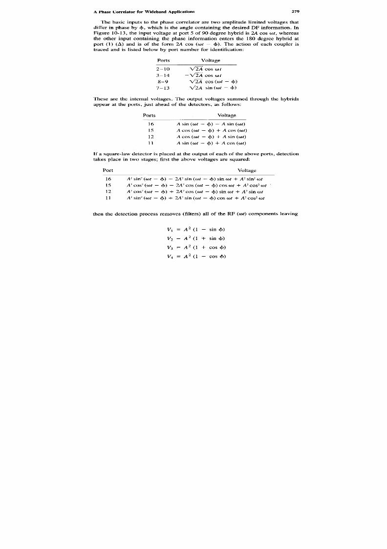
8/8/2019 SciTech - Microwave Passive Direction Finding
http://slidepdf.com/reader/full/scitech-microwave-passive-direction-finding 293/323
The basic inputs to the phase correlator are two amplitude limited voltages thatdiffer in phase by (J), which is the angle containing the desired DF information. InFigure 10-13, the input voltage at port 5 of 90 degree hybrid is 2A cos(ot, whereasthe other input containing the phase information enters the 180 degree hybrid atport (1) (A) and is of the form IA cos (cor - (J)). The action of each coupler istraced and is listed below by port number for identification:
Ports Voltage
2 - i o VIA COS cor3 -14 - V 2 A cos (o t8 -9 VlA COS (oof - (J))
7 -1 3 V 2A sin (oof - (J))
These are the internal voltages. The output voltages summed through the hybridsappear at the ports, just ahead of the detectors, as follows:
Ports Voltage
16 A sin ((ot — ()>)— A sin (oof)15 A cos ((Ot- ( ( ) ) + A cos((ot)12 A cos ((ot —c))) + A sin ((ot)11 A sin ((ot — 4>) H- A cos ((Ot)
If a square-law detector is placed at the output of each of the above ports, detectiontakes place in two stages; first the above voltages are squared:
Port Voltage
16 A2 sin2 ((ot - ( ( ) ) - 2A2 sin ((ot - (J)) sin (o t H- A2 sin2(o t15 A2 cos2 ((ot — <|>) — 2A2 cos ((ot - (J)) cos (o t + A2 cos2(o t12 A2 cos2 ((ot - ( ) ) ) + 2A2 cos (cor - (J)) sin(o t + A2 sin (O t11 A2 sin2 ((ot - (J)) 4- 2A2 sin ((ot —(J)) cos(o t + A2 cos2(o t
then the detection process removes (filters)all of the RF (oaf)components leaving
V1 = A2 (1 - sin (J))
V2 = A 2 (1 + sin (J))
V3 = A 2 (1 + cos (J))
V4 = A2 (1 - cos (J))

8/8/2019 SciTech - Microwave Passive Direction Finding
http://slidepdf.com/reader/full/scitech-microwave-passive-direction-finding 294/323
The outputs of the detectors are usually applied to four differential amplifiers,which provide the voltages:
V2 - Vi = 2A2 sin <$>
V3 - V4 = 2A2 cos (f)
The cosine channel is called the in-phase or / channel; the sine channel, thequadrature or Q channel. The ratio of HQ will give the tangent of $, and thedifferential outputs can be connected to a polar display to give the circular p-0display discussed above. The correlator for the purposes of passive direction-findingperforms an analog-to-digital conversion, converting the two voltages into a digitalword for the angle<\>. This is readily done by synchro-to-digital counters and zero-crossing detectors and is a standard digital technique.
The accuracy of the simple encoder shown here is limited by the signal-to-noiseratio of the signal presented to the detectors and the encoding accuracy, which isusually only 5 bits. In the frequency encoder, the correlator shown would onlyrepresent one set of digital numbers, the most significant bits, and would only beencoded to 25 = 32 places. A second discriminator, utilizing another longer delay
line, would have one ambiguity but would have a greater slope of degrees/MHz.This second channel would provide the next group of lesser significant bits, andthe process would continue with the addition of more encoders. In actual practice,an IFM usually has four delay line correlators oft, 4t, I6t, and 64?, and instantaneousfrequency measurement receivers can provide a 12-bit digital output. Systems ofthis type are called "gas-meter" encoders, in recognition of their similarity.
DF phase measurement utilizing multiple-fed arrays usually provides multiplephase angle $ outputs. This was shown for the circular array in Chapter 5, Section
5.4 , by moding the Butler-fed array so that <|>, 2 x c|>, 4 X <)>, and 8 X <|) wereavailable. The same technique is used in interferometers, as described in Chapter6. In this latter case, circuit phase comparisons are made to resolve theTV ambiguities.Phase encoders are generally preceded by an RF amplifier and hard (sharp knee)limiter to remove all amplitude va riation, since the detector outputs are proportionalto both the instantaneous amplitude and phase differences in the / andQ channels.The limiting action provides an amplitude-stripping action. Since limiting createsharm onics, any output harmonic power is subtracted from the fundamental. A signal
slightly weaker than the desired signal will therefore be rejected, the phenomenonbeing the well-known "capture effect."
Phase discriminators do suffer from accuracy problems in the presence of twonearly equal signals, whether pulse or CW. If the input signals differ by more than6 dB, the effects are minimal. The presence of jamming noise or a CW signal,however, can create inaccuracies and desensitization of the receiver. For thesereasons, phase discriminators are often preceded by tunable filters that can pass orreject bands of frequencies. The difficulties in instantaneous frequency measurementusing phase discriminators is gradually leading to the use of DF driven receiversand to the development of true digital instantaneous frequency encoders.

8/8/2019 SciTech - Microwave Passive Direction Finding
http://slidepdf.com/reader/full/scitech-microwave-passive-direction-finding 295/323
10.3 DFPROCESSING
Microwave passive DF provides the means to determine the angle-of-arrival of asignal from either a single pulse or from many pulses. In the first case, high signal-to-noise penalty must be paid; in the latter case, high precision accuracy can beachieved. The immediacy of the need for the information in part determines thesystem configuration. Processing of the DF intercept descriptor falls into two categoriesas we ll. First, there is the preprocessing that identifies that the signal is present andat a sufficient level to fall within accuracy, false alarm rate, and probability ofdetection criteria; that is, are the data usable? The second category uses the informationin various ways. ESM and signal intercept systems in the early 1970s used timedata such as pulse time-of-arrival and duration, amplitude, and DF as sortingparameters, since it was easy to determine the nature of a threat by the pulsegroupings, signal levels, and type of emitter scan. Frequency was used to identifythe band of operation, allowing the combination of parameters to be tested againsta priori data stored in a computer memory to provide threat identification. It wassimple to identify threats in a non-real-time environment since the design of threatradars were sufficiently different from friendly radars in pulse, scan, and modulationcharacteristics to permit fairly accurate characterizations. Unfortunately, as statedpreviously, the situation has changed; enemies became friends, friends becameenemies, and equipment from all sources began to become dispersed creating ho-mogeneous threat environments difficult to reduce to simple dimensions. The firstanswer was the addition of the IFM as an additional sorting word, and manyprocessors were designed to add pulse-by-pulse frequency as a signal tagging orcorrelating word. ESM equipment using this method is categorized as "frequencydriven" as stated many times throughout this book. The limited IFM encoder-correlator approach in many different configurations was perfected and available
for both base band (e.g., 2-6 GHz) and direct band (e.g., 2-8, 8-18 GHz)applications. This solution has carried ESM technology into the 1980s; however,new factors have elevated the DF descriptor into passive consideration.
Instantaneous frequency systems do not operate well in environments wherethere are many signals at amplitudes similar to the threats being detected. Thereshould be at least a 3-6 dB difference in amplitude for accurate measurements tobe made. In a light environment, the possibility of pulse coincidence is less thanin a heavy environment; but as time progresses, the environmental pulse densities
seem to increase. The presence of CW or high pulse repetition frequency (PRF)signals further exacerbate the problem. Although there are methods to recognizeand separate CW signals (11), and filters, such as using tunable YIGs to accept orreject desired and undesired signals, frequency has diminished somewhat as thekey sorting parameter. This trend has been accelerated by the proliferation offrequency agile and frequency diversive radar systems.
Direction-of-arrival, in contrast, has become more significant, with true monopulsebearing-taking becoming an important factor because the DF word is less difficultto measure with the availability of faster digital hardware and because DF cannotrapidly change. A threat can vary frequently very rapidly or use frequencies other

8/8/2019 SciTech - Microwave Passive Direction Finding
http://slidepdf.com/reader/full/scitech-microwave-passive-direction-finding 296/323
than usual to confuse frequency-driven receivers. Angle-of-arrival of a signal ishard to change quickly since it depends upon physical factors of the ballistics of amissile or a plane. It is admittedly hard to change DF quickly for ground targets.
Monopulse radar technology is another factor operating to enhance the use ofpassive direction finding to sort signals. As monopulse radars become deployedmore extensively, the use of scan modulation disappears (monopulse radars areconstant illuminators), and intercept signal scan cannot be used to sort signals. Theability to jam monopulse radars requires rapid response, and often DF data are theonly certain parameter available to "set-on" electronic countermeasures or to directchaff. In a contrasting sense, the improvement in RF sensitivities and the abilityto package greater computer aspects into warning or ELINT systems permits monopulseto be used more accurately for angle measurement.
A good example of DF technology is in the use of the interferometer receiver.It is clear that this type of system is capable of high resolution at the price of narrowbandwidths or of multiple ambiguities for wide-band applications. With the abilityto add computer assets and to combine amplitude and phase measurement techniques,these ambiguities can be resolved. Practical interferometer DF receivers are nowdeployed successfully. Many years have passed since the early interferometers weredeveloped, set aside, and redesigned using modern techniques. Much of the popularity
of the interferometer is in its ability to obtain accurate DF measurements.
10.3.1 Non-Real-Time DF Processing
DF determination processing is the implementation of the unambiguous measurementof the angle-of-arrival of a threat. This can be accomplished by comparison ofamplitudes (or phases) of adjacent channels if the signals in the two channels to becompared are at the proper signal-to-noise ratio. What should be done if they are
not? The answer is not always apparent; some systems reject both the strongest andnext strongest signals and wait for the next acceptable pulse pair. Other systemsindicate boresight reception in the direction of the strongest of two pulses with orwithout a flag to calibrate the measurement credibility. Som e systems average signalsand merely start a "track" or file of the possibility of a signal in a wide sector "b in ,"with hopes of reducing the bin size as more signals appear. Other more adaptivesystems look for other descriptors such as frequency or wait or retune to optimizethe situation.
A D F receiver may be reactive or adaptive depending upon the design ph ilosophy.The actual DF determination process usually starts with a recognition of the mostsignificant bit of the DF measurement, which can be simply recognition and codificationof the antenna that picked up the one pulse. The balance of the DF determinationwill make use of the direction-finding resolution capabilities of the receiver. In thecase of a rotating DF antenna, the receive bandwidth and pointing angle can beencoded; in monopulse systems, the ratio can be formed using amplitude and/orphase processor technology. In most cases, however, the DF word is formed inreal time and as quickly as possible. This is almost an absolute requirement for DF

8/8/2019 SciTech - Microwave Passive Direction Finding
http://slidepdf.com/reader/full/scitech-microwave-passive-direction-finding 297/323
driven systems and is part of the reason for the development of the pulse-on-pulsetechniques described above.
Figure 10-14 is another view of a generic receiver that operates in non-real time;that is, the output data is processed independently of the input data and is not timesynchronized with it. This type of system takes a picture in time of the signalenvironment and loads it into one-half of a temporary storage (usually a randomaccess mem ory, or mem ory (RAM ). Measurements are supplied to a threat memoryas a set of fields for DF, amplitude, time of arrival, and frequency either as an RFband (from RF multiplexed systems) or as a word (from an IFM). The suitabilityof a signal is then determined by a set of threshold detectors operating on then (inthis case four) DF outputs to indicate that the signal-to-noise thresholds have beencrossed and that a signal is suitable. Signals so judg ed are fed to the monopulseratioformer and the omni video and RF band analog-to-digital converters and tothe pulse wordformer where all immediately available information is grouped. Eachpulse group or set of fields is loaded into the active threat memoryhalf, whereasthe other half is operated on by the central processing unit (CPU). A nonvolatileprogram memory holds the algorithms for the CPU and, in the case of a warningreceiver, may be loaded prior to a mission. In the case shown here, two memoriesare used: One contains the program, the other the threat a priori database or "tele-phone direc tory." The CPU compares the static world of pulse fields until periodicityor match is obtained. The pulses are separated in non-real time and the parametersare compared to the a priori data for identification. If ambiguities arise, the processormay call for IFM frequency data, if only bands were used, or may classify thethreats as unknow n. The threat priority file keeps track of each threat and prioritizesthem by lethality and range for display.
As described above, the non-real-time system works well in moderate environments.DF determination is done in conjunction with the monopulse time available data
and can be used for sorting by using only the DF field as the sorting tool. Whenenvironments are dense and the switched memory system is unable to operate, DFinputs can be used to limit the sector of view to quadrants or octants to "wane" orthin the environment to permit the system to shed some of the work load. Accessto the DF system is usually available at the control indicator where limits can bemanually set. To do this the DF output word must be readily available. DF datawhen stored in the memory for computation and presentation must be in "true," ornorth reference, form since the host vehicle is usually constant motion , consequently
compass heading information is required. Since most monopulse ratioformers areanalog (subtractors, discriminators, etc.), an analog-to-digital conversion is oftenmade. Since intercept pulses of about 100 nanoseconds are expected, it is usuallydesirable to normalize all pulses to some wider standard width to permit a commonA-to-D conversion technique to be used. This can be done by the subtractor usedwith the DLVA or by the pulse-on-pulse DLVA by choice of the delay-line asexplained above. The phase correlation system provides a digital word directly sincein most phase monopulse systems, the development of the ratio is done in theencoding process. Frequency, in the form of a digital word, is requested by the

8/8/2019 SciTech - Microwave Passive Direction Finding
http://slidepdf.com/reader/full/scitech-microwave-passive-direction-finding 298/323
Figure 10-14. DF process functions in a non-
m n
f r e q
O m n iv i d e oA / D
P u l s e / R F b a nw o r d f o r m e r(A/D conver t e
g e t f r e q
d i g i t a lf r e g
M o n o p u l s er a t i of o r m e r
T h r e s h o l dd e t e c t o r
DLVA
IF M
A n ts y s t e m

8/8/2019 SciTech - Microwave Passive Direction Finding
http://slidepdf.com/reader/full/scitech-microwave-passive-direction-finding 299/323
computer to resolve ambiguities, and so on. IP7Ms take time (300 nanosecondstypically) and therefore are generally used by request in the DF driven system shownhere.
10.3.2 The Real-Time DF Sort Preprocessor
The DF word may be used as the first filter in the receiver as real-time sortingparam eter. To do this, our generic receiver is divided into preprocessor and processorsections. This restricts the information flow to the non-real-time processor on thebasis of real-time preprocessor filtering. Figure 10-15 shows the preprocessor conceptas used to filter data flow to the com puter. In this case, the subtle difference is thatevery pulse is DF tested against limitsbefore the data are passed to the computer.This reduces the computer loading. The monopulse pair is formed by a high-speedscan of the outputs of the DF antennas, or of a DF and omnidirectional antennapair, using DLVAs and two parallel receiver channels. A single channel supercom-mutated around then DF antennas within the width of a single pulse or a parallelchannel DF system w ith an analog sample-and-hold encoder can be used to providereal-time preprocessor DF data.
Since the DF sort preprocessor is designed to use the DF word as a decision
maker or to group or associate pulses by DF to reduce the computer work load,consistent DF measurements must be made on all signals. This requires high DFaccuracies, and consequent good signal-to-noise ratios for each pulse which reducessensitivity. A s a further aid, it is not unusual to add d igital correction to each angleon the basis of azimuth or frequency. Precalibration of the host vehicle is anothermeans to generate a usable azimuth-of-arrival correction data base.
10.3.3 Database Generation
Both of the above generic systems presuppose that a convenient telephone directoryof possible threats can be entered into the system for sorting intercepts. How is thistable directly developed? The answer is by electronic intelligence (ELINT) systems.The systems used for this purpose are large and usually unprogrammed at the start.
To controlindicatororcomputerto set oftracks
Data tothreatmemory
LimittestMono-pulsepair
HighspeedmonopulsescanDFants
Real timepulseA/Dconverter
Real tmeword former Switch
Figure 10-15. Preprocessor for real-time DF processing.
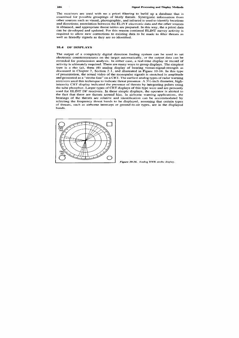
8/8/2019 SciTech - Microwave Passive Direction Finding
http://slidepdf.com/reader/full/scitech-microwave-passive-direction-finding 300/323
The receivers are used with no a priori filtering to build up a database that isexamined for possible groupings of likely threats. Synergistic information fromother sources such as visual, pho tographic, and infrared is used to identify locationsand directions; association between the ELINT electronic data and the other sourcesis obtained, and appropriate threat tables are prepared. In this way, the a priori datacan be developed and updated. For this reason continual ELINT survey activity isrequired to allow new corrections to existing data to be made to filter threats aswell as friendly signals as they are so identified.
10.4 DF DISPLAYS
The output of a completely digital direction finding system can be used to setelectronic countermeasures on the target automatically, or the output data can berecorded for postmission analysis. In either case, a real-time display or record ofactivity is ultimately required. There are many ways to group displays. The simplesttype is a rho (p), theta (6) analog display of bearing versus-signal-strength asdiscussed in Chapter 2, Section 2.1, and illustrated in Figure 10-16. In this typeof presentation, the actual video of the monopulse signals is stretched in amplitude
and presented as a "strobe line" on a CRT. The earliest analog types of radar warningreceivers used this technique to indicate threat presence. A SV^-inch diameter, h igh-intensity CRT display indicated the presence of threats by integrating pulses usingthe tube phosphor. Larger types of CR T displays of this type were and are presentlyused for ELINT DF receivers. In these simple displays, the operator is alerted tothe fact that there are threats around him. In airborne warning applications, thebearings of the threats are relative and identification can be accommodated byselecting the frequency threat bands to be displayed, assuming that certain types
of threats, such as airborne intercept or ground-to-air types, are in the displayedbands.
Figure 10-16. Analog RWR strobe display.
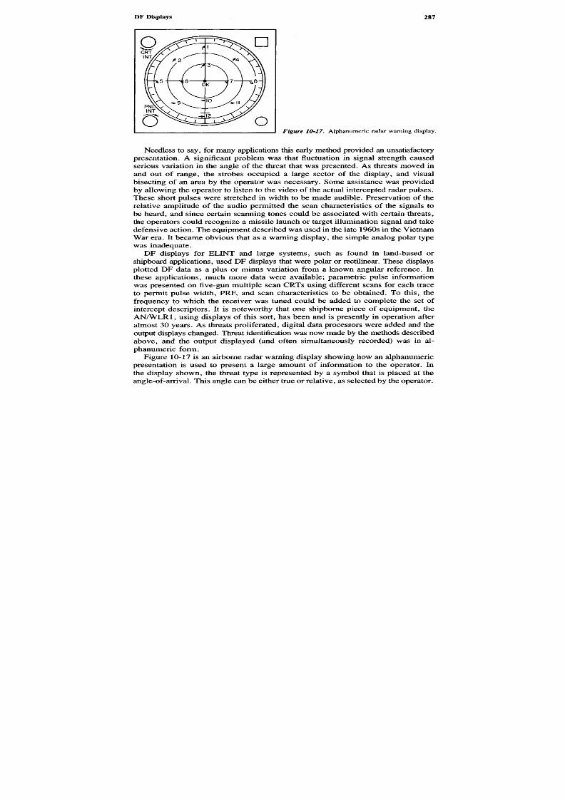
8/8/2019 SciTech - Microwave Passive Direction Finding
http://slidepdf.com/reader/full/scitech-microwave-passive-direction-finding 301/323
Needless to say, for many applications this early method provided an unsatisfactorypresentation. A significant problem was that fluctuation in signal strength causedserious variation in the angle of the threat that was presented. As threats moved inand out of range, the strobes occupied a large sector of the display, and visualbisecting of an area by the operator was necessary. Some assistance was providedby allowing the operator to listen to the video of the actual intercepted radar pulses.These short pulses were stretched in width to be made audible. Preservation of therelative amplitude of the audio permitted the scan characteristics of the signals tobe heard, and since certain scanning tones could be associated with certain threats,the operators could recognize a missile launch or target illumination signal and takedefensive action. T he equipm ent described w as used in the late 1960s in the VietnamWar era. It became obvious that as a warning display, the simple analog polar type
was inadequate.DF displays for ELINT and large systems, such as found in land-based orshipboard applications, used DF displays that were polar or rectilinear. These displaysplotted DF data as a plus or minus variation from a known angular reference. Inthese applications, much more data were available; parametric pulse informationwas presented on five-gun multiple scan CRTs using different scans for each traceto permit pulse width, PRF, and scan characteristics to be obtained. To this, thefrequency to which the receiver was tuned could be added to complete the set of
intercept descriptors. It is noteworthy that one shipborne piece of equipment, theAN/WLR1, using displays of this sort, has been and is presently in operation afteralmost 30 years. As threats proliferated, digital data processors were added and theoutput displays changed. Threat identification was now made by the methods describedabove, and the output displayed (and often simultaneously recorded) was in al-phanumeric form.
Figure 10-17 is an airborne radar warning display showing how an alphanumericpresentation is used to present a large amount of information to the operator. Inthe display shown, the threat type is represented by a symbol that is placed at theangle-of-arrival. This angle can be either true or relative , as selected by the operator.
Figure 10-17. Alphanumeric radar warning display.

8/8/2019 SciTech - Microwave Passive Direction Finding
http://slidepdf.com/reader/full/scitech-microwave-passive-direction-finding 302/323
The lethality of the signal, represented by its signal strength, is indicated by theradial distance from the outer edge, the graticule circles representing increasingpriority. Thus a threat in the center circle would be of the greatest concern. Inaddition, the status of the threats acquisition and control systems, as determinablefrom its modulation , is indicated by symbol blinking and an audio alarm. Add itionalthreat-type information is shown by the arrow indicators. If the display becomescongested (many threats in one quadrant), the lesser priority threats are dropped orthe display can be expanded to show multiple signals at a given crowded azimuthsector. This type of display is typically of high brightness to permit viewing in asunlit aircraft cockpit.
ELINT displays also make use of digitally processed data. A typical display can
be polar as discussed above; but since more screen space is available in a rectangularformat, positional D F data display is not generally used . Figure 10-18 is a frequency-azimuth threat display found in large systems. This display is a frequency-azimuthpresentation showing alphanumeric identified threats as they range from a bore-sight azimuth (along the abscissa) at the frequency of occurrence (on the ordinate).The identity of the threat is designated by the symbol denoting recognition of theclass of threat represented. A cursor controlled by a joystick hooks any individual
Figure 10-18. Frequency-azimuth threat display.
DISPLAYAND
CURSOR E-A P

8/8/2019 SciTech - Microwave Passive Direction Finding
http://slidepdf.com/reader/full/scitech-microwave-passive-direction-finding 303/323
threat by encircling it as shown. A parametric readout of the encircled threat isdisplayed in the corner and is recorded together with header information consistingof date, time, mission number, vehicle location, and so on, for postmission analysis.The frequency-azimuth display finds favor in shipboard systems since the boresightcan be made to represent the forward direction or locus of travel of the ship. Thisis a convenient way to identify angle quadrants quickly and permits evasive ma-neuvering or countermeasures to be used.
R E F E R E N C E S
1. Hughes, R. S., "Make Very Wide-Range Log Amps Easily,"Electronic D esign,Oct. 11, 1970,pp. 76 ff.
2. Hughes, R. S., Logarithmic Video Amplifiers,Dedham, MA: Artech House, 1971.
3. Morgan, D., "Get the Most Out of Log Amplifiers by Understanding Error Sources,"ElectronicDesign News,Jan. 20, 1973, pp. 52 ff.
4. Potson, D., and R. Hughes, "Extremely Fast Log Amp Handles Narrow Pulses,"Microwaves &RF, Apr. 1985, p. 85.
5. Potson, D., and R. Hughes, "DC-Coupled Video Log Amp Processes 10-ns Pulses,"Microwaves& RF, May 1985, Part II, p. 75.
6. Barber, W., and E. Brown, "A True Logarithmic Amplifier for Radar IF Applications,"IEEEJournal of Solid State Circuits,Vol. SC 15, No. 3, June 1980, p. 291.
7. Lan sdow ne, K., and D . No rton, "Log Amplifiers Solve Dynam ic-Range and Rapid-Pulse ResponseProblems," Microwave Systems News,Oct. 1985, pp. 99 ff.
8. Wilkens, M. W. and W.. R. Kincheloe, Jr., "Microwave Realization of Broadband Phase andFrequency Discriminators," Stanford Electronics Labs, Technical Report 1962/1966-2-SU-SEL 68-057, Stanford, CA, 1968.
9. Lipsky, S. E., "Measure New Threat Frequencies Instantly,"Microwaves,Dec. 1970.
10.Gysel, IL, and J. P. Watjen, "Wide-Band Frequency Discriminator with High Linearity,"
IEEEMTT-S Internal Microwave Symposium Digest,1977.
11 . Tsui, J., and G. Schrick, "Instantaneous Frequency Measurement Receiver to Separate Pulse andCW Signals," U.S. Patent 4,1194,206, Mar. 18, 1980.

8/8/2019 SciTech - Microwave Passive Direction Finding
http://slidepdf.com/reader/full/scitech-microwave-passive-direction-finding 304/323
Future Trends
Microwave passive direction finding has been presented here in many different
forms and many different ways. As originally stated, the purpose of this book hasbeen to trace both the development of direction finding from its origins and toexplain and describe the means of the technology to permit interested engineers tofind the methods of the technique in one place. Any book covering as many aspectsas I have tried to do undoubtedly raises questions. Some can be answered by moreresearch, some by intensive study of the references, some only by the future actingas a driving force.
The rapid development of solid-state devices capable of developing RF energy
at high microwave frequencies has resulted in small, high-gain, active transmittingand RF receiving antenna array systems. These arrays will permit high-effectiveradiated power to be generated by multiple aperture antennas, which will requirehigh-accuracy, steered-beam receivers for seton. Such systems presently exist andare becoming deployed in many new applications. Small size is a natural fallout,and it is reasonab le to expect printed circuit RF techniques to become more prevalentfor both the circuitry and radiating elements. Evidence of this trend is clear inpresent literature, with the strong emphasis on microstrip and "patch" antennatechnology. Adaptive array systems are also being developed to optimize theseconcepts.
Passive DF accuracy has become an important targeting or aiming tool, forcingDF accuracy to be improved. These accuracy trends for future radar warning orESM systems place emphasis on built-in antenna and receiver systems, using bothamplitude and phase interferometer techniques to measure and sort signals on atrue monopulse basis. Most new electronic support measures receivers includeinstantaneous frequency measurement of baseband downconverted signals to provideadditional intercept sorting and recognition capability. The trend in processing has
Chapter Eleven

8/8/2019 SciTech - Microwave Passive Direction Finding
http://slidepdf.com/reader/full/scitech-microwave-passive-direction-finding 305/323

8/8/2019 SciTech - Microwave Passive Direction Finding
http://slidepdf.com/reader/full/scitech-microwave-passive-direction-finding 306/323
will be dedicated to defensive electronic warfare for the good of all. To this goal,this book has been dedicated.
R E F E R E N C E
1. John son, D ., "The App lication of Spectral Estimation Methods to the Bearing Estimation P roble m ."Proc.IEEE, 1982, pp. 1018-1028.

8/8/2019 SciTech - Microwave Passive Direction Finding
http://slidepdf.com/reader/full/scitech-microwave-passive-direction-finding 307/323
293 This page has been reformatted by Knovel to provide easier navigation.
Index
Index terms Links
A
Accuracy:
channel unbalance 242of DF systems 233
Adaptive array 127
Adcock 3
Adjacency rule 104 235 241
Alphanumeric display 106
Amplifier:
compressive 9
log video 263
Amplitude monopulse, definition 27
Amplitude noise accuracy 248
Amplitude-weighted phase shift 129
AN/ALR-80 106
Anaren circular antenna array 135
Angular articulation 27 102 117 133
159 160 165 166
235
Antector 59Antenna:
active region 55
the Antector 59
axial ratio 38 59
beamformer 123
biconical horn 77 bootlace 138

8/8/2019 SciTech - Microwave Passive Direction Finding
http://slidepdf.com/reader/full/scitech-microwave-passive-direction-finding 308/323
294
Index terms Links
This page has been reformatted by Knovel to provide easier navigation.
Antenna: (Continued)
conformal 123
dual-mode excitation 57dynamic range 13
E-plane patterns 37
half-omni 78 122 130
Honey-Jones 81
H-plane patterns 37
passive detection arrays 128 planar equiangular spiral 48
polarization 37
ports 139
self-complementary 57
slow-wave 44
spiral:
active region 55
band theory 46 55
cavity backed 41
circular 41
conical equiangular logarithmic 53
even-mode radiation 46 56
four-arm 57
millimeter wave 59
multiple-arm 57
normal mode 47
odd-mode radiation 46 56
planar archimedian 41 43
planar equiangular 41
six-arm 57 59
squint 46
Antenna arrays 126
Antenna depolarization 261Antenna gain 38 75

8/8/2019 SciTech - Microwave Passive Direction Finding
http://slidepdf.com/reader/full/scitech-microwave-passive-direction-finding 309/323
295
Index terms Links
This page has been reformatted by Knovel to provide easier navigation.
Antiradiation technique 9
Aperture 6
APR-39A 106Arc antenna 143
Archer 141 146
Archimedian spiral 43
Array pattern 129
Articulation, see Angular articulation
Auto-correlation 171
Axial ratio balance 248
Ayer 181 185
B
Babinet’s principle 40Balun transformer 50
Baseband noise 187
Baseband receiver 203
Baseline array 166
Beamformer ports 139
Beaming ambiguity 14
Beam-on-beam 223 226 231
Beam-on-beam antenna probability 207
Beamwidth, variation in accuracy 244
Biconical horn radiator 81
Binary-beam interferometer 166Biphase modulator 120
Blass 130 140
Bootlace antenna 138
Boresight 6
Built-in test facilities (BITE) 233
Butler array 130

8/8/2019 SciTech - Microwave Passive Direction Finding
http://slidepdf.com/reader/full/scitech-microwave-passive-direction-finding 310/323
296
Index terms Links
This page has been reformatted by Knovel to provide easier navigation.
Butler circular array 259 277
Butler matrix 132
C
Capture effect 280
Cavity backed spiral 41
Central processing unit (CPU) 283
Characteristic impedance 69
Circle of error probability (CEP) 101
Circular Butler-fed array 132
Circular interferometer 165 168
Circular pattern 38
Circular polarization 38 76
Circular waveguide 72Co-boresighting 224
Collocated 7
Communications intelligence (COMINT) 291
Compressive amplifiers 9
Compressive logarithmic video amplifier 263
Confining gain 191 193 195
definition 186
Conformal mount 130 165 168
Constant FAR 216
Constant illuminator 112 282
Cross polarization loss 38Crossover loss 246 248
Crystal video receiver (CVR) 172
CW Chopping 102
D
Database 285
Data reduction 10
8/8/2019 SciTech - Microwave Passive Direction Finding
http://slidepdf.com/reader/full/scitech-microwave-passive-direction-finding 311/323
297
Index terms Links
This page has been reformatted by Knovel to provide easier navigation.
dBm, definition 8
Decommutator 116
Deinterleaving 105 116 Depth-of-penetration 71
Desensitization 267 280
Detection integration 219
Detector:
back-diode 179
boxcar 111
figure-of-merit 177
hot-carrier diode 179
sample-and-hold 111
Schottky diode 179
square law 173
tunnel diode 179
Detector law 174
Detector logarithmic video amplifier (DLVA) 264
DF displays 286
DF-driven receivers 106 119 172 205
280 DF look-up tables 130
DF processing, non-real time 282
Digital instantaneous frequency encoders 280
Diodes, point-contact silicon 178
Direction finding roots 11
Directional pattern 3
Dispersed antennas 234 257 259
Display:
alphanumeric 287
frequency-azimuth 288
rectilinear 287 rho-theta 287

8/8/2019 SciTech - Microwave Passive Direction Finding
http://slidepdf.com/reader/full/scitech-microwave-passive-direction-finding 312/323
298
Index terms Links
This page has been reformatted by Knovel to provide easier navigation.
Distributed source technique 127
DLVA 17 31 168 222
264 283 Doppler, moving-target indicators 126
Double attenuation 8
Double-ridged horns 130
Double sideband (DSB) 194
Down-conversion superheterodyne 197
Downconverter receiver 203
Down-time 10
DRAM memory 117
Dual baseline interferometer 160
Duty cycle 264
Dwell time 117Dynamic random access memory (DRAM) 117
Dynamic video resistance 176
E
EEPROM memory 106
Effective bandwidth 181
Effective radiated power (ERP) 124
Electronically steered beam 128
Electronic Intelligence (ELINT) 9
Electronic order of battle (EOB) 9 101
Electronic support measures (ESM) 10 126Elemental current excitation 133
Element factor 129
Elevation angle 15
ELINT 1 123 150 171
231 282 285 291
See also Electronic Intelligence (ELINT)Elisra Corp. 147

8/8/2019 SciTech - Microwave Passive Direction Finding
http://slidepdf.com/reader/full/scitech-microwave-passive-direction-finding 313/323
299
Index terms Links
This page has been reformatted by Knovel to provide easier navigation.
Elliptical paraboloid reflector 93
Elliptical polarization 261
Entropy 101Envelope detector 209
EOB 101
See also Electronic order of battle (EOB)
E-plane patterns 37
Equiangular planar spiral 49
Error function (erf) 212
ESM 281
See also Electronic support measures (ESM)
F
False alarm probability 208False alarm rate (FAR), denned 190 208 210 212
216 221
False triggering 201
Filter, band separation 102
Filters 195
Five-port turnstile junction 87
Frequency-driven receiver 114 208 281
Frequency scan probability 226
G
Gain-limited 186 187 196
Gain-limited crystal video receiver 175
Gain-limited receiver 173 178 186
Gaussian 182 210 215 222
Gaussian antenna 241
Gaussian antenna pattern 238
Gaussian antenna pattern approximation 234

8/8/2019 SciTech - Microwave Passive Direction Finding
http://slidepdf.com/reader/full/scitech-microwave-passive-direction-finding 314/323
300
Index terms Links
This page has been reformatted by Knovel to provide easier navigation.
Gaussian noise distribution 188 250
Generic receiver 283
GENT 138Geographical antenna dispersement 130
Glint 235
Goniometer 5
Grating lobes 122 261
Ground clutter 87
H
Half-omnidirectional antennas 70 123 130
Hatcher 229
Homodyne receiver 191 194 202
Honey-Jones antenna 81 234Horn antennas, horn types 68
Horns:
E-plane 75
H-plane 75
pyramidal 75
sectorial 75
H-plane 15
H-plane patterns 37
Hughes 191 267 269
Hybrid directional coupler 27
Hyperfast tuning 172
See also Microscan
I
IF bandwidth 196
IFM 166 168 277 281
See also Instantaneous frequency measurement (IFM)Image-cancellation mixers 201

8/8/2019 SciTech - Microwave Passive Direction Finding
http://slidepdf.com/reader/full/scitech-microwave-passive-direction-finding 315/323
301
Index terms Links
This page has been reformatted by Knovel to provide easier navigation.
Image frequency 196
Image response 195
Inertialess scan 128Information bandwidth 196
Installation accuracy 256
Instantaneous frequency measurement (IFM) 32 114
Intercept probability 223
Interferometer 55 108 155 156
160 254 280 282
Interferometer ambiguities 160
Interferometer arrays 167
Isotropic radiator 38
KKinchloe 229
Klipper 183
L
Lens-fed array 9 138 139
See also Rotman lensLimiter 102
Linear detector 198 212 215 222
Linear superheterodyne 197
Lobe-on-receive-only (LORO) 112
Log amplifier:
hybrid design 272
pulse-on-pulse type 270
series sequential design 269
successive detection type 275
Log amplifier compression ratio, definition 268
Logarithmic amplifier 9 16 102 117123 222 250 263

8/8/2019 SciTech - Microwave Passive Direction Finding
http://slidepdf.com/reader/full/scitech-microwave-passive-direction-finding 316/323
302
Index terms Links
This page has been reformatted by Knovel to provide easier navigation.
Logarithmic IF amplifier 110 201
Logarithmic RF amplifier 263 272
Logarithmic video amplifier 198 263Look-up table 10 105 241 245
247
LORO 112
Lucas 183
MMagic-T directional coupler 27
MARCHAND balun 50 59
Matched polarization 38
Mathematics of interferometry 156
Maximum linear sequence 120Microscan 172 191 229
Microstrip 81
Millimeter wave radars 223
Millimeter wave range 11 291
Millimeter wave spirals 59
Mode separation filter 83 84 85 87
Mode suppressor 92
Monochannel monopulse 119
Monopulse 6 7 19 23
24 119 120 157
167 196 231 250
277
Monopulse angle determination 29
Monopulse postulates 25
Monopulse processor:
Class I 30
Class II 30 168Class III 32

8/8/2019 SciTech - Microwave Passive Direction Finding
http://slidepdf.com/reader/full/scitech-microwave-passive-direction-finding 317/323
303
Index terms Links
This page has been reformatted by Knovel to provide easier navigation.
Monopulse radar 282
Monostatic 6 7
Monser 146Multibeam DF arrays 123
Multidimensional array 127
Multimode and multiarm spirals 55
Multimode DF horn 79
Multipath interferences 86
Multiple-aperture systems 165
Multiple-arm spiral 57
Multiple baseline interferometer 168
Multiplexer 102 241
N Noise:
chi-square case 212
definition of 171
flicker 176
Gaussian 182
shot 176spectrum 194
thermal 176
Noise figure (F), definition 192
Noise-limited receiver 119 122 181 182
186 188 196 209
219 221
Noise probability density function 210
Nonharmonic-related 166
Nonideality factor 176
Nonisotropic 3
Nonvolatile program memory 283

8/8/2019 SciTech - Microwave Passive Direction Finding
http://slidepdf.com/reader/full/scitech-microwave-passive-direction-finding 318/323
304
Index terms Links
This page has been reformatted by Knovel to provide easier navigation.
Normalization 23 114 157 208
224 263
Nutating 6 Nyquist criteria 117
O
Occupancy bandwidth 119
Odd mode 61
Omniazimuthal multibeam array 147
Omniazimuthal, see Omnidirectional
Omnidirectional 3 15 24 81
114 120 130 135
224
P
Parallel-beam array 128
Parallel beam-formed arrays 129
Parallel beam septum antenna 147
Parallel compare 117
Parallel DF channelization 122Parametric readout 289
Passive detection 2
Passive detection arrays 128
Passive direction finding 8
Passive lobing 7 126
Passive reflector 93
Pencil beam raster 76
PFA 212
See also Probability of false alarm
Phase and sum-and-difference monopulse 107
Phase correlator 32 277

8/8/2019 SciTech - Microwave Passive Direction Finding
http://slidepdf.com/reader/full/scitech-microwave-passive-direction-finding 319/323
305
Index terms Links
This page has been reformatted by Knovel to provide easier navigation.
Phase dispersion 87
Phase encoders, gas meter 280
Phase monopulse, definition 27Phase monopulse systems 283
Phase noise accuracy 252
Phase tagging monopulse 120
Plan position indication (PPI) 6
Planar archimedian spiral 41
Planar array 127
Planar Butler array 130
Planar equiangular spiral 41
Planar spiral antenna 50
Point-contact silicon diodes 178
Polar display 13Polarization 37
Polarizer, meander-line 91
Polar map 6
Power-managed countermeasures 207
Pozar 142
Preamplification 104
Predetection amplification 104
Preprocessor, real-time DF sort 285
Preprocessor comparator 117
Preselector bandwidth 196
Preselector loss 195Presorting 10
PRF 281
See also Pulse repetition frequency (PRF)
PRI 6 226
Prioritized threat file 105
Probability of detection 207 231

8/8/2019 SciTech - Microwave Passive Direction Finding
http://slidepdf.com/reader/full/scitech-microwave-passive-direction-finding 320/323
306
Index terms Links
This page has been reformatted by Knovel to provide easier navigation.
Probability of false alarm 210
Processing gain 10 171
Pseudomonopulse 112 Pseudomonopulse receiver 111 113
Pulse, back porch 9
Pulse-on-pulse DLVA 283
Pulse overlap 102
Pulse repetition frequency (PRF) 13
Pulsewidth, minimum 216
Q
Quadraplexing 102 104
Quadratic detection 212 221 222
R
Rabbit ears 201
Radar warning receiver (RWR) 1 102
generic 102
Rayleigh distribution 210
Rayleigh’s reciprocity theorem 73
Range gating 7 126
Raster scan 128
Receiver:
baseband 203
DF-driven 106 119
frequency-driven 114
noise-limiter 119 122
subcommutated 114
subcommutated pseudomonopulse 114
Reciprocity theorem 139
Recovery time 264 266 271 275 Rectangular waveguide 69

8/8/2019 SciTech - Microwave Passive Direction Finding
http://slidepdf.com/reader/full/scitech-microwave-passive-direction-finding 321/323
307
Index terms Links
This page has been reformatted by Knovel to provide easier navigation.
Reflector antennas 92
Refresh time, definition 171
Repeater jammers 9Retrodirective 123 126 139
Retrodirective DF 9
RF transmission lines 68
Rice 183
Ridged waveguide 72
Rise time 196
R-KR lens 143
R-KR multiband antenna 261
RMS error for a DF system 245
Rotating DF intercept probability 224
Rotating reflector antennas 93Rotman lens 139
design equations 142
Rotman phased/array antenna 124
Rotman-Turner 140
Rule of adjacency 104
RWR, frequency-driven 114
See also Radar warning receiver (RWR)
S
Sampling 102 116
Scanning 6Schottky diode 179
Scintillation 7
Self-complementary 40 49 57
Sequenced offset-pair system 116
Sequenced/pair switching 114
Sequential lobing 6 7

8/8/2019 SciTech - Microwave Passive Direction Finding
http://slidepdf.com/reader/full/scitech-microwave-passive-direction-finding 322/323
308
Index terms Links
This page has been reformatted by Knovel to provide easier navigation.
Shadow time 10 267 271
definition 171
Short baseline interferometer 165Sidelobe inhibitor 15
Sidelobe response 13
Signal averaging 171
Signal detection in noise 213
Signal intercept system 281
Signal lethality 288
Signal-to-noise ratios 198
Signal-to-noise sensitivity methods 187
Sine antenna pattern 234
Single baseline 156
Single sideband (SSB) noise figure 194Six-arm spiral 59
Skirt inhibition 17
Skirt-inhibitor 201
Skolnik 209 210
Slant linear polarization 38 76 81
Small signal suppression effect 183
S/N ratio 188
Spiral antenna 39
See also Antenna, spiral
Split-taper feed 50
Spurious signals 195Square-law 219 222
Square-law CVR 180
Square-law detector 212 216
Square spiral 44
Squint 46 50 52 241
242
Squint accuracy 244

8/8/2019 SciTech - Microwave Passive Direction Finding
http://slidepdf.com/reader/full/scitech-microwave-passive-direction-finding 323/323
309
Index terms Links
This page has been reformatted by Knovel to provide easier navigation.
Steered-receive linear arrays 151
Stripline 81 92
Strobe line 286Subcommutated receiver 114
Subcommutation 112
Subcommutation methods 111
Successive detection logarithmic IF amplifier 263
Sum-and-difference ( Σ – ∆ ) 25
definition 27
Sum-and-difference interferometer 109
Supercommutation 116 117
Superheterodyne receiver 191
Switched-antenna systems 150
Switched-beam array 128 150Switched-lobe receiver 111
Switched-lobe technique 112
Switched phaseshift array 9
Synergistic information 286
System adaptation 171
T
Tangential sensitivity (TSS) 184 186 190
definition 173
Tapered coaxial feedline 50
Targeting 126Target location 3
Threat memory 283
Time-delay beamformer 139
Time-division multiplexing (TDM) 119
Track-while-scan (TWS) 7 24
Triangulation 3
True DF 283