scoring functions for learning bayesian networksasmc/pub/talks/09-ta/ta_pres.pdf · scoring...
TRANSCRIPT
Scoring functions for learningBayesian networks
Alexandra M. Carvalho
Topicos Avancados – p. 1/48

Plan
Learning Bayesian networks
Scoring functions for learning Bayesian networks:
Bayesian scoring functions:BD (Bayesian Dirichlet) (1995)BDe ("‘e"’ for likelihood-equivalence) (1995)BDeu ("‘u"’ for uniform joint distribution) (1991)K2 (1992)
Information-theoretic scoring functions:LL (Log-likelihood) (1912-22)MDL/BIC (Minimum description length/Bayesian Information Criterion) (1978)AIC (Akaike Information Criterion) (1974)NML (Normalized Minimum Likelihood) (2008)MIT (Mutual Information Tests) (2006)
Decomposability and score equivalence
Experiments
Conclusion
Topicos Avancados – p. 2/48
Bayesian networks
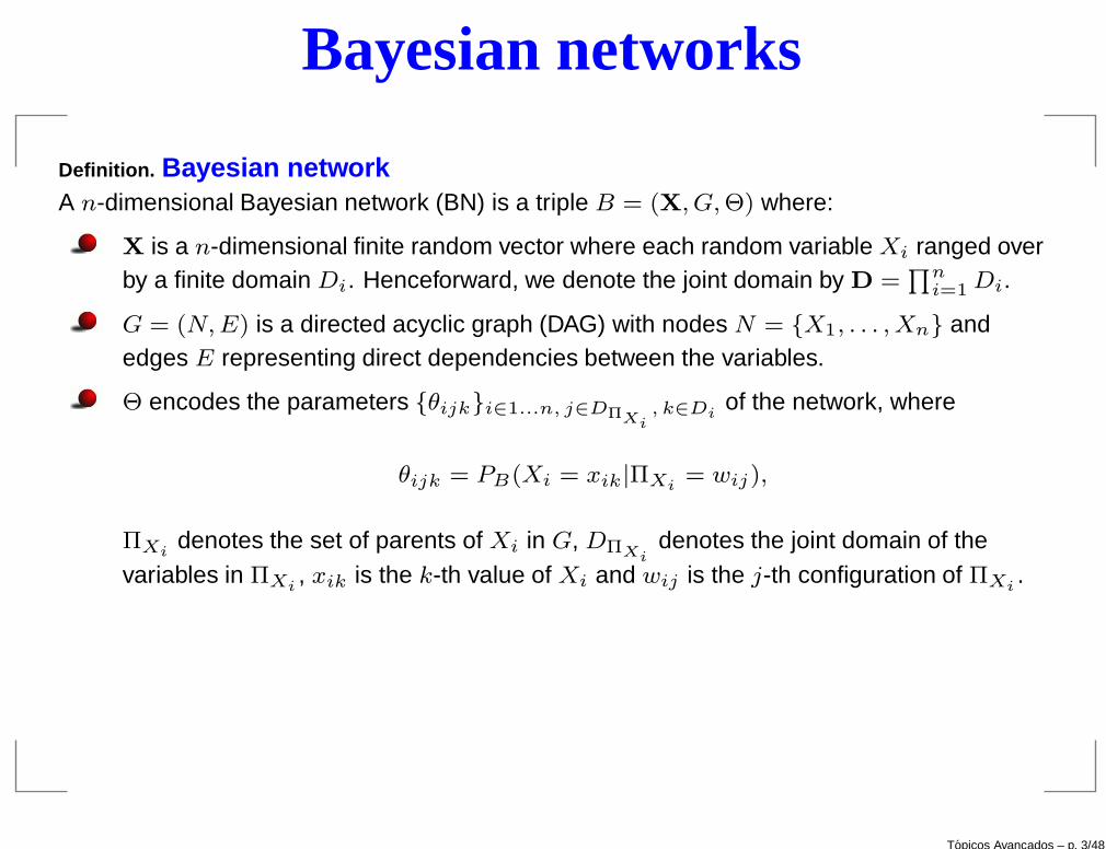
Definition. Bayesian networkA n-dimensional Bayesian network (BN) is a triple B = (X, G, Θ) where:
X is a n-dimensional finite random vector where each random variable Xi ranged overby a finite domain Di. Henceforward, we denote the joint domain by D =
∏ni=1 Di.
G = (N, E) is a directed acyclic graph (DAG) with nodes N = {X1, . . . , Xn} andedges E representing direct dependencies between the variables.
Θ encodes the parameters {θijk}i∈1...n, j∈DΠXi, k∈Di
of the network, where
θijk = PB(Xi = xik|ΠXi= wij),
ΠXidenotes the set of parents of Xi in G, DΠXi
denotes the joint domain of thevariables in ΠXi
, xik is the k-th value of Xi and wij is the j-th configuration of ΠXi.
Topicos Avancados – p. 3/48
Bayesian networks
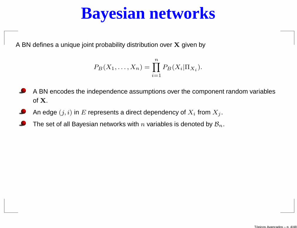
A BN defines a unique joint probability distribution over X given by
PB(X1, . . . , Xn) =n∏
i=1
PB(Xi|ΠXi).
A BN encodes the independence assumptions over the component random variablesof X.
An edge (j, i) in E represents a direct dependency of Xi from Xj .
The set of all Bayesian networks with n variables is denoted by Bn.
Topicos Avancados – p. 4/48
Learning Bayesian networks
Learning a BN:
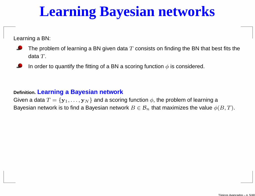
The problem of learning a BN given data T consists on finding the BN that best fits thedata T .
In order to quantify the fitting of a BN a scoring function φ is considered.
Definition. Learning a Bayesian networkGiven a data T = {y1, . . . ,yN} and a scoring function φ, the problem of learning aBayesian network is to find a Bayesian network B ∈ Bn that maximizes the value φ(B, T ).
Topicos Avancados – p. 5/48

Hardness results
Cooper (1990) showed that the inference of a general BN is a NP-hard problem.=⇒ APPROXIMATE SOLUTIONS
Dagum and Luby (1993) showed that even finding an approximate solution is NP-hard.=⇒ RESTRICT SEARCH SPACE
First attempts confined the network to tree structures and used Edmonds (1967)and Chow-Liu (1968) optimal branching algorithms to learn the network.
More general classes of BNs have eluded efforts to develop efficient learningalgorithms.
Chickering (1996) showed that learning the structure of a BN is NP-hard even fornetworks constrained to have in-degree at most 2.
Dasgupta (1999) showed that even learning 2-polytrees is NP-hard.
Due to these hardness results exact polynomial-time bounded approaches for learningBNs have been restricted to tree structures.
Topicos Avancados – p. 6/48
Standard methodology
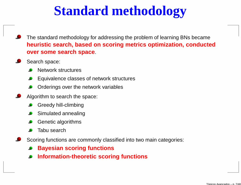
The standard methodology for addressing the problem of learning BNs becameheuristic search, based on scoring metrics optimization, c onductedover some search space .
Search space:
Network structures
Equivalence classes of network structures
Orderings over the network variables
Algorithm to search the space:
Greedy hill-climbing
Simulated annealing
Genetic algorithms
Tabu search
Scoring functions are commonly classified into two main categories:
Bayesian scoring functionsInformation-theoretic scoring functions
Topicos Avancados – p. 7/48
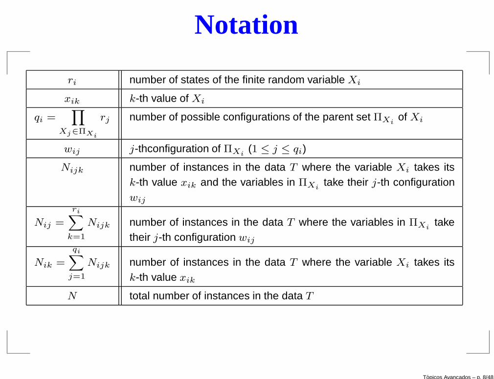
Notation
ri number of states of the finite random variable Xi
xik k-th value of Xi
qi =∏
Xj∈ΠXi
rj number of possible configurations of the parent set ΠXiof Xi
wij j-thconfiguration of ΠXi(1 ≤ j ≤ qi)
Nijk number of instances in the data T where the variable Xi takes itsk-th value xik and the variables in ΠXi
take their j-th configurationwij
Nij =
ri∑
k=1
Nijk number of instances in the data T where the variables in ΠXitake
their j-th configuration wij
Nik =
qi∑
j=1
Nijk number of instances in the data T where the variable Xi takes itsk-th value xik
N total number of instances in the data T
Topicos Avancados – p. 8/48
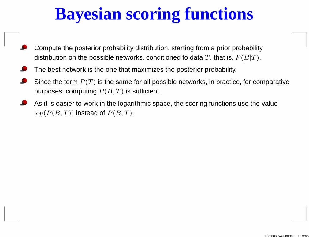
Bayesian scoring functions
Compute the posterior probability distribution, starting from a prior probabilitydistribution on the possible networks, conditioned to data T , that is, P (B|T ).
The best network is the one that maximizes the posterior probability.
Since the term P (T ) is the same for all possible networks, in practice, for comparativepurposes, computing P (B, T ) is sufficient.
As it is easier to work in the logarithmic space, the scoring functions use the valuelog(P (B, T )) instead of P (B, T ).
Topicos Avancados – p. 9/48
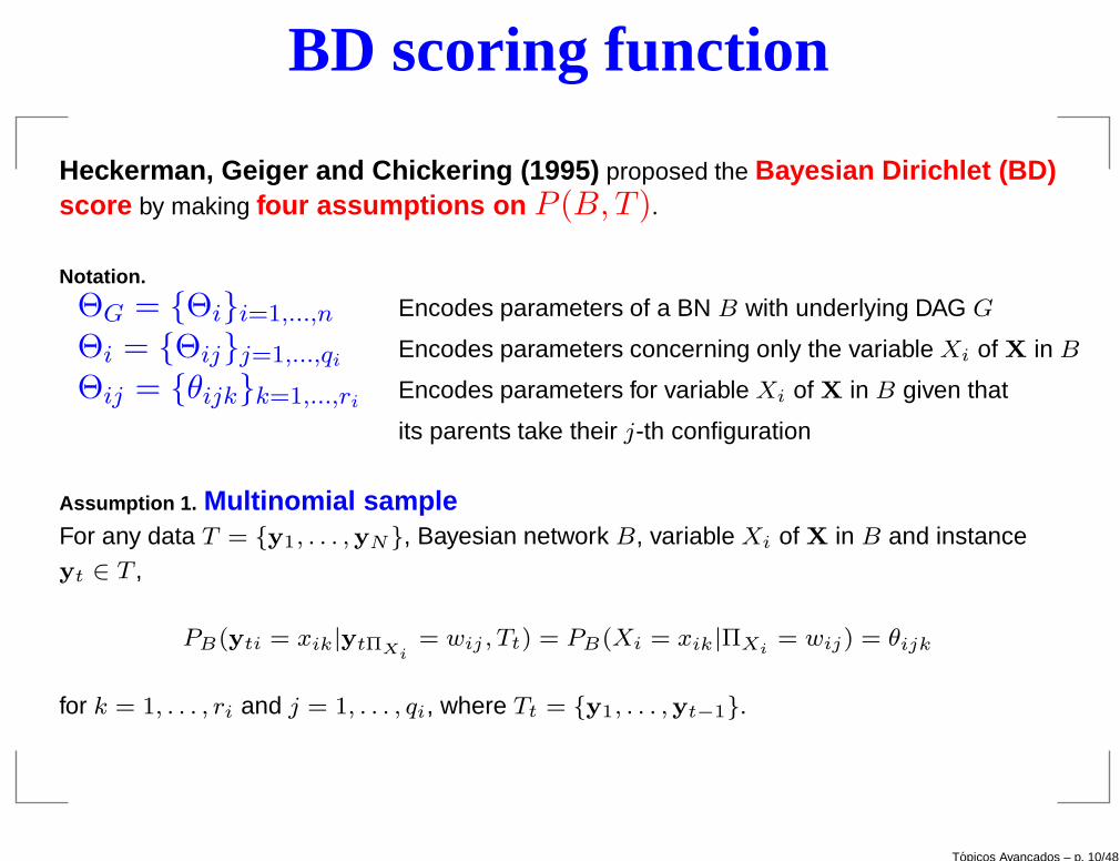
BD scoring function
Heckerman, Geiger and Chickering (1995) proposed the Bayesian Dirichlet (BD)score by making four assumptions on P (B,T ).
Notation.
ΘG = {Θi}i=1,...,n Encodes parameters of a BN B with underlying DAG G
Θi = {Θij}j=1,...,qiEncodes parameters concerning only the variable Xi of X in B
Θij = {θijk}k=1,...,riEncodes parameters for variable Xi of X in B given that
its parents take their j-th configuration
Assumption 1. Multinomial sampleFor any data T = {y1, . . . ,yN}, Bayesian network B, variable Xi of X in B and instanceyt ∈ T ,
PB(yti = xik|ytΠXi= wij , Tt) = PB(Xi = xik|ΠXi
= wij) = θijk
for k = 1, . . . , ri and j = 1, . . . , qi, where Tt = {y1, . . . ,yt−1}.
Topicos Avancados – p. 10/48
BD scoring function
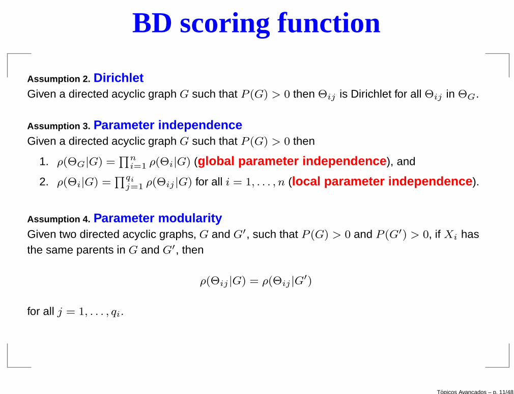
Assumption 2. DirichletGiven a directed acyclic graph G such that P (G) > 0 then Θij is Dirichlet for all Θij in ΘG.
Assumption 3. Parameter independenceGiven a directed acyclic graph G such that P (G) > 0 then
1. ρ(ΘG|G) =∏n
i=1 ρ(Θi|G) (global parameter independence ), and
2. ρ(Θi|G) =∏qi
j=1 ρ(Θij |G) for all i = 1, . . . , n (local parameter independence ).
Assumption 4. Parameter modularityGiven two directed acyclic graphs, G and G′, such that P (G) > 0 and P (G′) > 0, if Xi hasthe same parents in G and G′, then
ρ(Θij |G) = ρ(Θij |G′)
for all j = 1, . . . , qi.
Topicos Avancados – p. 11/48
BD scoring function
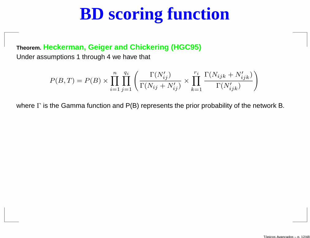
Theorem. Heckerman, Geiger and Chickering (HGC95)Under assumptions 1 through 4 we have that
P (B, T ) = P (B) ×n∏
i=1
qi∏
j=1
(
Γ(N ′ij)
Γ(Nij + N ′ij)
×
ri∏
k=1
Γ(Nijk + N ′ijk
)
Γ(N ′ijk
)
)
where Γ is the Gamma function and P(B) represents the prior probability of the network B.
Topicos Avancados – p. 12/48

BD scoring function
The HGC95 theorem induces the Bayesian Dirichlet (BD) score :
BD(B, T ) = log(P (B)) +n∑
i=1
qi∑
j=1
(
log
(
Γ(N ′ij)
Γ(Nij + N ′ij)
)
+
ri∑
k=1
log
(
Γ(Nijk + N ′ijk
)
Γ(N ′ijk
)
))
.
The BD score is unusable in practice:
Specifying all hyperparameters N ′ijk
for all i, j and k is formidable, to say the least.
There are some particular cases of the BD score that are useful...
Topicos Avancados – p. 13/48

K2 scoring function
Cooper and Herskovits (1992) proposed a particular case of the BD score, called theK2 score ,
K2(B, T ) = log(P (B)) +n∑
i=1
qi∑
j=1
(
log
(
(ri − 1)!
(Nij + ri − 1)!
)
+
ri∑
k=1
log(Nijk!)
)
,
with the uninformative assignment N ′ijk
= 1 (corresponding to zero pseudo-counts).
Topicos Avancados – p. 14/48

BDe scoring function
Heckerman, Geiger and Chickering (1995) turn around the problem ofhyperparameter specification by considering two additional assumptions: likelihoodequivalence and structure possibility .
Definition. Equivalent directed acyclic graphsTwo directed acyclic graphs are equivalent if they can encode the same joint probabilitydistributions.
Given a Bayesian network B, data T can be seen as a multinomial sample of the joint spaceD with parameters
ΘD = {θx1...xn}xi=1,...,ri, i∈1...n
where θx1...xn =∏n
i=1 θxi|Πxi.
Assumption 5. Likelihood equivalenceGiven two directed acyclic graphs, G and G′, such that P (G) > 0 and P (G′) > 0, if G andG are equivalent then ρ(ΘD|G) = ρ(ΘD|G′).
Topicos Avancados – p. 15/48
BDe scoring function
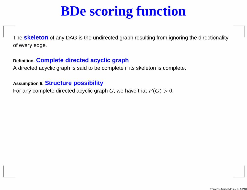
The skeleton of any DAG is the undirected graph resulting from ignoring the directionalityof every edge.
Definition. Complete directed acyclic graphA directed acyclic graph is said to be complete if its skeleton is complete.
Assumption 6. Structure possibilityFor any complete directed acyclic graph G, we have that P (G) > 0.
Topicos Avancados – p. 16/48
BDe scoring function
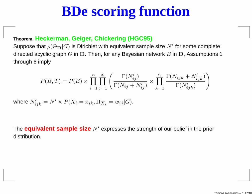
Theorem. Heckerman, Geiger, Chickering (HGC95)Suppose that ρ(ΘD|G) is Dirichlet with equivalent sample size N ′ for some completedirected acyclic graph G in D. Then, for any Bayesian network B in D, Assumptions 1through 6 imply
P (B, T ) = P (B) ×n∏
i=1
qi∏
j=1
(
Γ(N ′ij)
Γ(Nij + N ′ij)
×
ri∏
k=1
Γ(Nijk + N ′ijk
)
Γ(N ′ijk
)
)
where N ′ijk
= N ′ × P (Xi = xik, ΠXi= wij |G).
The equivalent sample size N ′ expresses the strength of our belief in the priordistribution.
Topicos Avancados – p. 17/48

BDe scoring function
The HGC95 theorem induces the likelihood-equivalence Bayesian Dirichlet (BDe)score and its expression is identical to the BD expression.
The BDe score is of little practical interest:
It requires knowing P (Xi = xik, ΠXi= wij |G) for all i, j and k, which might not be
elementary to find.
Topicos Avancados – p. 18/48

BDeu scoring function
Buntine (1991) proposed a particular case of BDe score, called the BDeu score :
BDeu(B, T ) = log(P (B))+n∑
i=1
qi∑
j=1
log
Γ( N′
qi)
Γ(Nij + N′
qi)
+
ri∑
k=1
log
Γ(Nijk + N′
riqi)
Γ( N′
riqi)
,
which appears when
P (Xi = xik, ΠXi= wij |G) =
1
riqi
.
This score only depends on one parameter, the equivalent sample size N ′:
Since there are no generally accepted rule to determine the hyperparametersN ′
x1...xn, there is no particular good candidate for N ′.
In practice, the BDeu score is very sensitive with respect to the equivalent sample sizeN ′ and so, several values are attempted.
Topicos Avancados – p. 19/48

Information-theoretic scoring functions
Information-theoretic scoring functions are based on compression:
The score of a Bayesian network B is related to the compression that can be achievedover the data T with an optimal code induced by B.
Shannon’s source coding theorem (or noiseless coding theorem) establishes thelimits to possible data compression .
Theorem. Shannon source coding theoremAs the number of instances of an i.i.d. data tends to infinity, no compression of the data ispossible into a shorter message length than the total Shannon entropy, without losinginformation.
Several optimal codes asymptotically achieve Shannon’s limit:
Fano-Shannon code and Huffman code , for instance.
Building such codes requires a probability distribution over data T .
Topicos Avancados – p. 20/48
Information-theoretic scoring functions
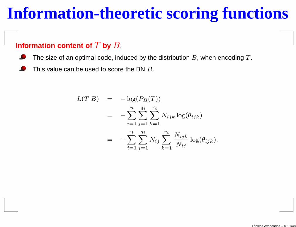
Information content of T by B:
The size of an optimal code, induced by the distribution B, when encoding T .
This value can be used to score the BN B.
L(T |B) = − log(PB(T ))
= −n∑
i=1
qi∑
j=1
ri∑
k=1
Nijk log(θijk)
= −n∑
i=1
qi∑
j=1
Nij
ri∑
k=1
Nijk
Nij
log(θijk).
Topicos Avancados – p. 21/48
Information-theoretic scoring functions
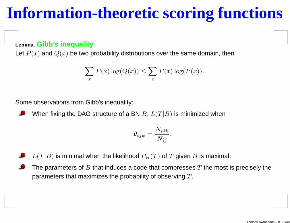
Lemma. Gibb’s inequalityLet P (x) and Q(x) be two probability distributions over the same domain, then
∑
x
P (x) log(Q(x)) ≤∑
x
P (x) log(P (x)).
Some observations from Gibb’s inequality:
When fixing the DAG structure of a BN B, L(T |B) is minimized when
θijk =Nijk
Nij
.
L(T |B) is minimal when the likelihood PB(T ) of T given B is maximal.
The parameters of B that induces a code that compresses T the most is precisely theparameters that maximizes the probability of observing T .
Topicos Avancados – p. 22/48

LL scoring function
The log-likelihood (LL) score is defined in the following way:
LL(B|T ) =n∑
i=1
qi∑
j=1
ri∑
k=1
Nijk log
(
Nijk
Nij
)
.
The LL score tends to favor complete network structures and it does not provide anuseful representation of the independence assumptions of the learned network.
This phenomenon of overfitting is usually avoided in two different ways:
By limiting the number of parents per network variable.
By using some penalization factor over the LL score:MDL/BIC (Occam’s razor approach)AICNML (Stochastic complexity)
Topicos Avancados – p. 23/48

MDL scoring function
The minimum description length (MDL) score is an Occam’s razor approach tofitting, preferring simple BNs over complex ones:
MDL(B|T ) = LL(B|T ) −1
2log(N)|B|,
where
|B| =n∑
i=1
(ri − 1)qi
denotes the network complexity , that is, the number of parameters in Θ for the networkB.
The first term of the MDL score measures how many bits are needed to describe dataT based on the probability distribution PB .
The second term of the MDL score represents the length of describing the network B,that is, it counts the number of bits needed to encode B, where 1
2log(N) bits are used
for each parameter in Θ.
Topicos Avancados – p. 24/48
AIC/BIC scoring function
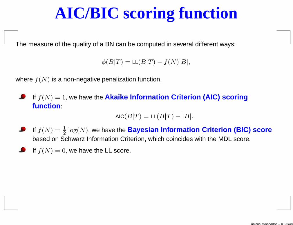
The measure of the quality of a BN can be computed in several different ways:
φ(B|T ) = LL(B|T ) − f(N)|B|,
where f(N) is a non-negative penalization function.
If f(N) = 1, we have the Akaike Information Criterion (AIC) scoringfunction :
AIC(B|T ) = LL(B|T ) − |B|.
If f(N) = 12
log(N), we have the Bayesian Information Criterion (BIC) scorebased on Schwarz Information Criterion, which coincides with the MDL score.
If f(N) = 0, we have the LL score.
Topicos Avancados – p. 25/48

NML scoring function
Recently, Roos, Silander, Konthanen and Myllym aki (2008) , proposed a newscoring function based on the MDL principle.
Insights about the MDL principle:
To explain data T one should always choose the hypothesis with smallest descriptionthat generates T .
What is a description and its length ?
First candidate: Kolmogorov complexity of T , that is, the size of the smallestprogram that generates T written in a fixed universal programming language.
Kolmogorov complexity is undecidable.
The size of the description depends on the chosen programming language.
Topicos Avancados – p. 26/48
NML scoring function
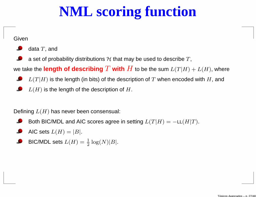
Given
data T , and
a set of probability distributions H that may be used to describe T ,
we take the length of describing T with H to be the sum L(T |H) + L(H), where
L(T |H) is the length (in bits) of the description of T when encoded with H, and
L(H) is the length of the description of H.
Defining L(H) has never been consensual:
Both BIC/MDL and AIC scores agree in setting L(T |H) = −LL(H|T ).
AIC sets L(H) = |B|.
BIC/MDL sets L(H) = 12
log(N)|B|.
Topicos Avancados – p. 27/48
NML scoring function
Using |B| in the expression of the complexity of a BN is, in general, an error:
The parameters of a BN are conditional distributions. Thus, if there are probabilities inΘ taking value 0, they do not need to appear in the description of Θ.
The same distribution (or probability value) might occur several times in Θ leading topatterns that can be exploited to compress Θ significantly.
There have been attempts to correct L(H):
Most of the works are supported more on empirical evidence than on theoreticalresults.
The main breakthrough in the community was to consider normalized minimumlikelihood codes .
Topicos Avancados – p. 28/48
NML scoring function
The idea behind normalized minimum likelihood codes is the same of universal coding :
Suppose an encoder is about to observe data T which he plans to compress as muchas possible.
The encoder has a set of candidate codes H and he believes one of these codes willallow to compress the incoming data significantly.
However, he has to choose the code before observing the data.
In general, there is no code which, no mater what incoming data T is, will alwaysmimic the best code for T .
So what is the best thing that the encoder can do?
There are simple solutions to this problem when H is finite, however, this is not thecase for BNs.
Topicos Avancados – p. 29/48
NML scoring function
Recasting the problem in a stochastic wording:
Given a set of probability distributions H the encoder thinks that there is onedistribution H ∈ H that will assign high likelihood (low code length) to the incomingdata T of fixed size N .
We woukd like to design a code that for all T will compress T as close as possible tothe code associated to H ∈ H that maximizes the likelihood of T .
We call to this H ∈ H the best-fitting hypothesis .
We can compare the performance of a distribution H w.r.t. H ′ of modeling T ofsize N by computing
− log(P (T |H)) + log(P (T |H′)).
Topicos Avancados – p. 30/48
NML scoring function
Given a set of probability distributions H and a distribution H not necessarily in H, the
regret of H relative to H for T of size N is
− log(P (T |H)) − minH∈H
(− log(P (T |H))).
In many practical cases, given a set of hypothesis H and data T , we are always able to findthe HH(T ) ∈ H that minimizes − log(P (T |H)):
The regret of H relative to H for T of size N can be rewritten as
− log(P (T |H)) + log(P (T |HH(T ))).
Topicos Avancados – p. 31/48
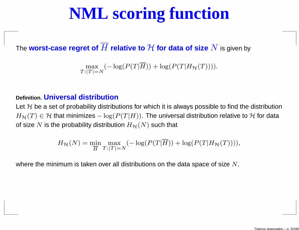
NML scoring function
The worst-case regret of H relative to H for data of size N is given by
maxT :|T |=N
(− log(P (T |H)) + log(P (T |HH(T )))).
Definition. Universal distributionLet H be a set of probability distributions for which it is always possible to find the distributionHH(T ) ∈ H that minimizes − log(P (T |H)). The universal distribution relative to H for dataof size N is the probability distribution HH(N) such that
HH(N) = minH
maxT :|T |=N
(− log(P (T |H)) + log(P (T |HH(T )))),
where the minimum is taken over all distributions on the data space of size N .
Topicos Avancados – p. 32/48

NML scoring function
The parametric complexity of H for data of size N is
CN (H) = log
∑
T :|T |=N
P (T |HH(T ))
.
Theorem. Shtakov (1987)Let H be a set of probability distributions such that CN (H) is finite. Then, the universaldistribution relative to H for data of size N is given by
P NMLH (T ) =
P (T |HH(T ))∑
T ′:|T ′|=N P (T ′|HH(T ′)).
The distribution P NMLH (T ) is called the normalized maximum likelihood (NML)
distribution.
Topicos Avancados – p. 33/48
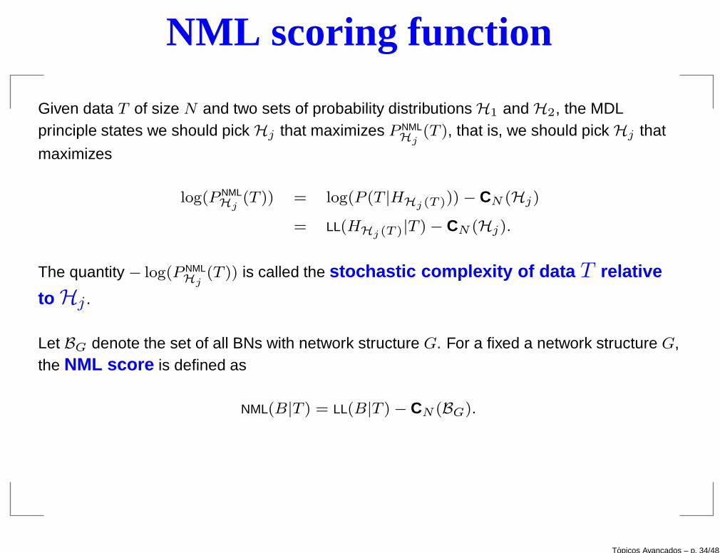
NML scoring function
Given data T of size N and two sets of probability distributions H1 and H2, the MDLprinciple states we should pick Hj that maximizes P NML
Hj(T ), that is, we should pick Hj that
maximizes
log(P NMLHj
(T )) = log(P (T |HHj(T ))) − CN (Hj)
= LL(HHj(T )|T ) − CN (Hj).
The quantity − log(P NMLHj
(T )) is called the stochastic complexity of data T relative
to Hj .
Let BG denote the set of all BNs with network structure G. For a fixed a network structure G,the NML score is defined as
NML(B|T ) = LL(B|T ) − CN (BG).
Topicos Avancados – p. 34/48
NML scoring function
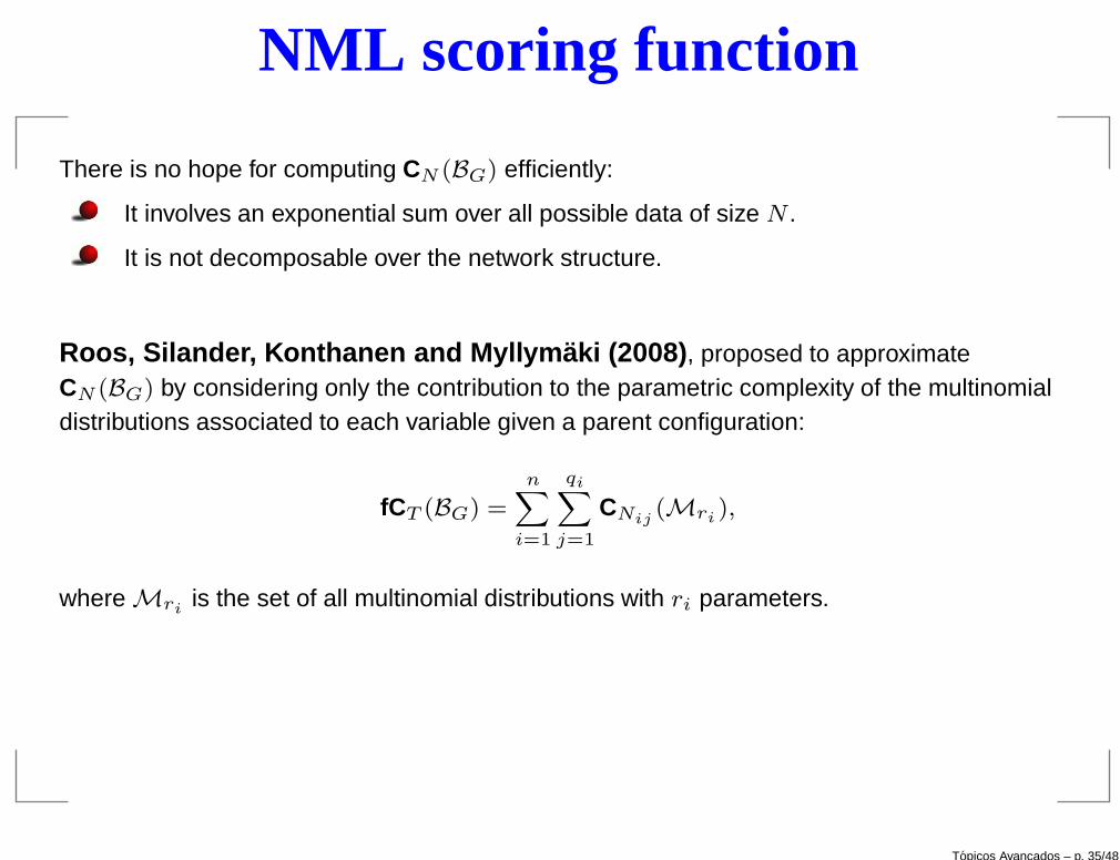
There is no hope for computing CN (BG) efficiently:
It involves an exponential sum over all possible data of size N .
It is not decomposable over the network structure.
Roos, Silander, Konthanen and Myllym aki (2008) , proposed to approximateCN (BG) by considering only the contribution to the parametric complexity of the multinomialdistributions associated to each variable given a parent configuration:
fCT (BG) =n∑
i=1
qi∑
j=1
CNij(Mri
),
where Mriis the set of all multinomial distributions with ri parameters.
Topicos Avancados – p. 35/48
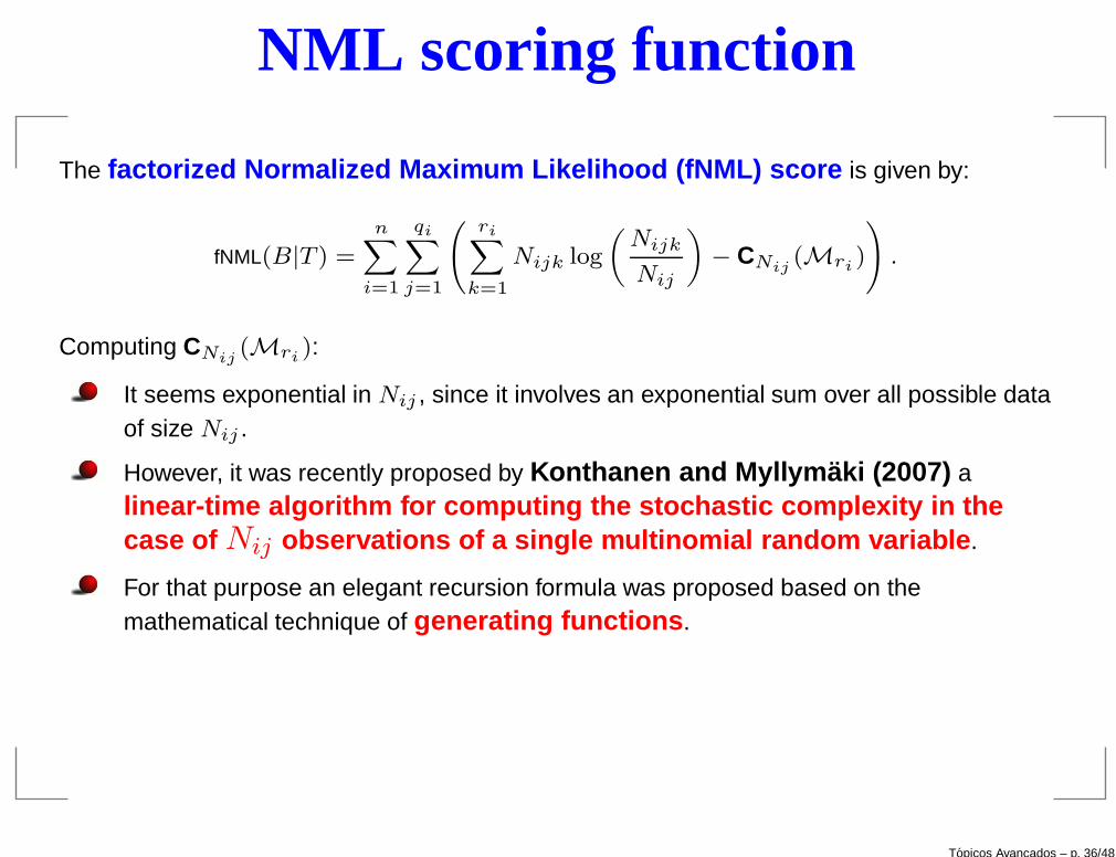
NML scoring function
The factorized Normalized Maximum Likelihood (fNML) score is given by:
fNML(B|T ) =n∑
i=1
qi∑
j=1
(
ri∑
k=1
Nijk log
(
Nijk
Nij
)
− CNij(Mri
)
)
.
Computing CNij(Mri
):
It seems exponential in Nij , since it involves an exponential sum over all possible dataof size Nij .
However, it was recently proposed by Konthanen and Myllym aki (2007) alinear-time algorithm for computing the stochastic comple xity in thecase of Nij observations of a single multinomial random variable .
For that purpose an elegant recursion formula was proposed based on themathematical technique of generating functions .
Topicos Avancados – p. 36/48

MIT scoring function
A scoring function based on mutual information, called mutual information tests (MIT)score , was proposed by de Campos (2006) and its expression is given by
MIT(B|T ) =n∑
i=1ΠXi
6=∅
2NI(Xi; ΠXi) −
si∑
j=1
χα,liσ∗
i(j)
,
where I(Xi; ΠXi) is the mutual information between Xi and ΠXi
in the network whichmeasures the degree of interaction between each variable and its parents.
Topicos Avancados – p. 37/48
MIT scoring function
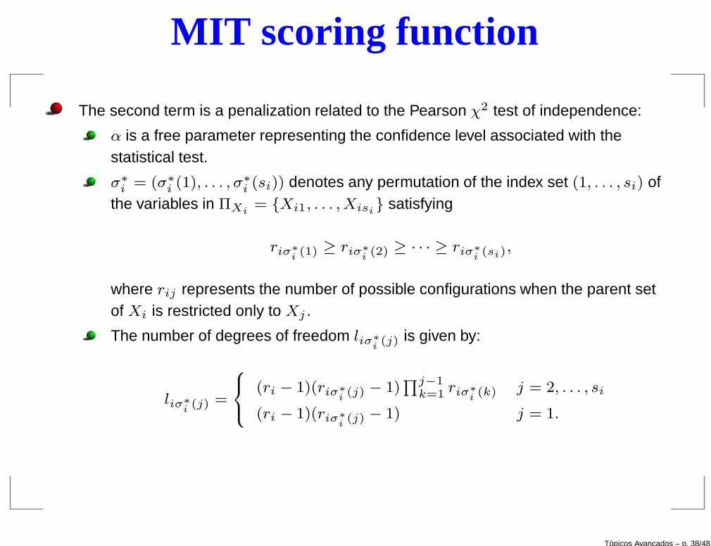
The second term is a penalization related to the Pearson χ2 test of independence:
α is a free parameter representing the confidence level associated with thestatistical test.
σ∗i = (σ∗
i (1), . . . , σ∗i (si)) denotes any permutation of the index set (1, . . . , si) of
the variables in ΠXi= {Xi1, . . . , Xisi
} satisfying
riσ∗
i(1) ≥ riσ∗
i(2) ≥ · · · ≥ riσ∗
i(si),
where rij represents the number of possible configurations when the parent setof Xi is restricted only to Xj .
The number of degrees of freedom liσ∗
i(j) is given by:
liσ∗
i(j) =
(ri − 1)(riσ∗
i(j) − 1)
∏j−1k=1 riσ∗
i(k) j = 2, . . . , si
(ri − 1)(riσ∗
i(j) − 1) j = 1.
Topicos Avancados – p. 38/48
Experiments
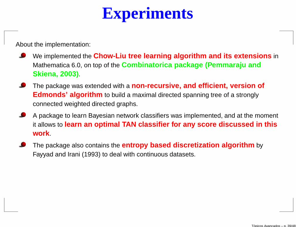
About the implementation:
We implemented the Chow-Liu tree learning algorithm and its extensions inMathematica 6.0, on top of the Combinatorica package (Pemmaraju andSkiena, 2003) .
The package was extended with a non-recursive, and efficient, version ofEdmonds’ algorithm to build a maximal directed spanning tree of a stronglyconnected weighted directed graphs.
A package to learn Bayesian network classifiers was implemented, and at the momentit allows to learn an optimal TAN classifier for any score discussed in thi swork .
The package also contains the entropy based discretization algorithm byFayyad and Irani (1993) to deal with continuous datasets.
Topicos Avancados – p. 39/48
Experiments
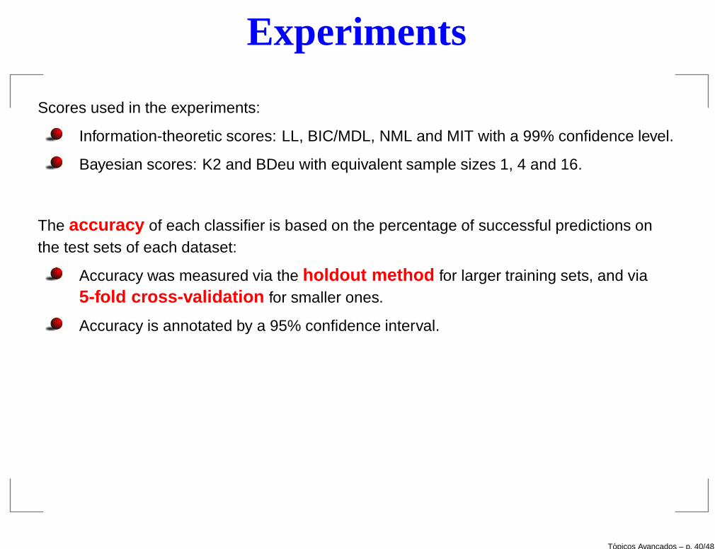
Scores used in the experiments:
Information-theoretic scores: LL, BIC/MDL, NML and MIT with a 99% confidence level.
Bayesian scores: K2 and BDeu with equivalent sample sizes 1, 4 and 16.
The accuracy of each classifier is based on the percentage of successful predictions onthe test sets of each dataset:
Accuracy was measured via the holdout method for larger training sets, and via5-fold cross-validation for smaller ones.
Accuracy is annotated by a 95% confidence interval.
Topicos Avancados – p. 40/48
Experiments
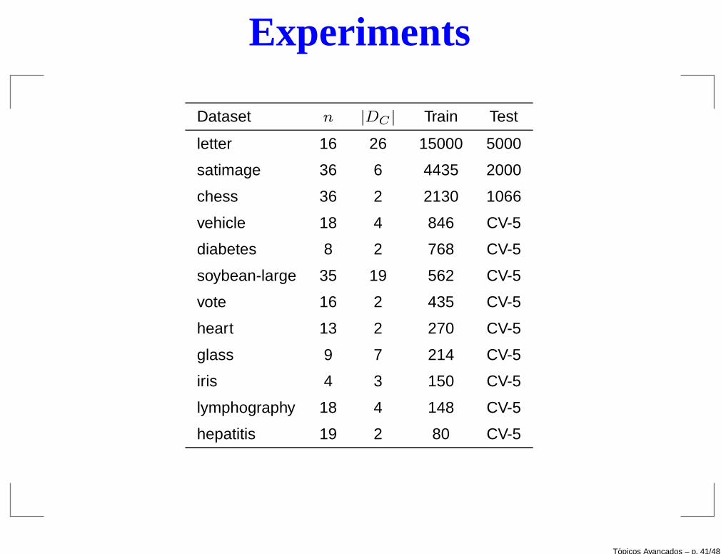
Dataset n |DC | Train Test
letter 16 26 15000 5000
satimage 36 6 4435 2000
chess 36 2 2130 1066
vehicle 18 4 846 CV-5
diabetes 8 2 768 CV-5
soybean-large 35 19 562 CV-5
vote 16 2 435 CV-5
heart 13 2 270 CV-5
glass 9 7 214 CV-5
iris 4 3 150 CV-5
lymphography 18 4 148 CV-5
hepatitis 19 2 80 CV-5
Topicos Avancados – p. 41/48
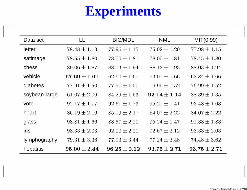
Experiments
Data set LL BIC/MDL NML MIT(0.99)
letter 78.48 ± 1.13 77.96 ± 1.15 75.02 ± 1.20 77.98 ± 1.15
satimage 78.55 ± 1.80 78.00 ± 1.81 78.00 ± 1.81 78.45 ± 1.80
chess 89.06 ± 1.87 88.03 ± 1.94 88.13 ± 1.93 88.03 ± 1.94
vehicle 67.69 ± 1.61 62.60 ± 1.67 63.07 ± 1.66 62.84 ± 1.66
diabetes 77.91 ± 1.50 77.91 ± 1.50 76.99 ± 1.52 76.99 ± 1.52
soybean-large 61.07 ± 2.06 84.29 ± 1.53 92.14 ± 1.14 88.39 ± 1.35
vote 92.17 ± 1.77 92.61 ± 1.73 95.21 ± 1.41 93.48 ± 1.63
heart 85.19 ± 2.16 85.19 ± 2.17 84.07 ± 2.22 84.07 ± 2.22
glass 93.81 ± 1.66 88.57 ± 2.20 95.24 ± 1.47 92.38 ± 1.83
iris 93.33 ± 2.03 92.00 ± 2.21 92.67 ± 2.12 93.33 ± 2.03
lymphography 79.31 ± 3.36 77.93 ± 3.44 77.24 ± 3.48 74.48 ± 3.62
hepatitis 95.00 ± 2.44 96.25 ± 2.12 93.75 ± 2.71 93.75 ± 2.71
Topicos Avancados – p. 42/48
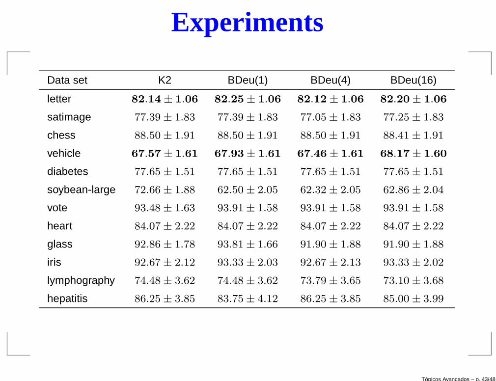
Experiments
Data set K2 BDeu(1) BDeu(4) BDeu(16)
letter 82.14 ± 1.06 82.25 ± 1.06 82.12 ± 1.06 82.20 ± 1.06
satimage 77.39 ± 1.83 77.39 ± 1.83 77.05 ± 1.83 77.25 ± 1.83
chess 88.50 ± 1.91 88.50 ± 1.91 88.50 ± 1.91 88.41 ± 1.91
vehicle 67.57 ± 1.61 67.93 ± 1.61 67.46 ± 1.61 68.17 ± 1.60
diabetes 77.65 ± 1.51 77.65 ± 1.51 77.65 ± 1.51 77.65 ± 1.51
soybean-large 72.66 ± 1.88 62.50 ± 2.05 62.32 ± 2.05 62.86 ± 2.04
vote 93.48 ± 1.63 93.91 ± 1.58 93.91 ± 1.58 93.91 ± 1.58
heart 84.07 ± 2.22 84.07 ± 2.22 84.07 ± 2.22 84.07 ± 2.22
glass 92.86 ± 1.78 93.81 ± 1.66 91.90 ± 1.88 91.90 ± 1.88
iris 92.67 ± 2.12 93.33 ± 2.03 92.67 ± 2.13 93.33 ± 2.02
lymphography 74.48 ± 3.62 74.48 ± 3.62 73.79 ± 3.65 73.10 ± 3.68
hepatitis 86.25 ± 3.85 83.75 ± 4.12 86.25 ± 3.85 85.00 ± 3.99
Topicos Avancados – p. 43/48
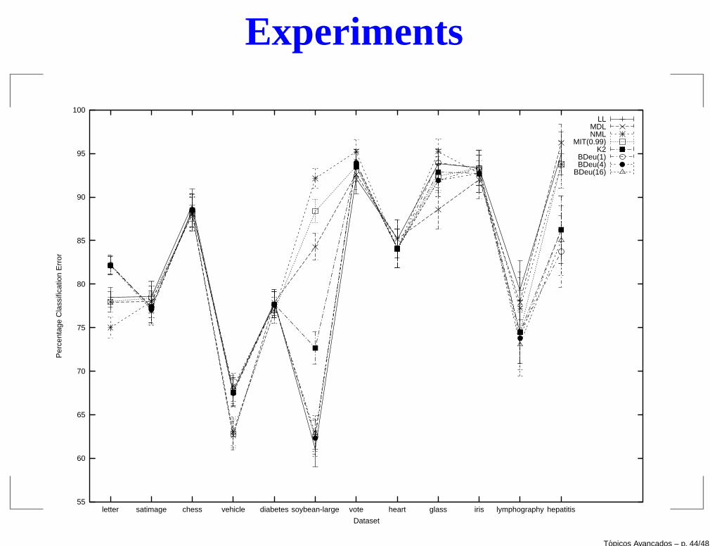
Experiments
55
60
65
70
75
80
85
90
95
100
hepatitislymphographyirisglassheartvotesoybean-largediabetesvehiclechesssatimageletter
Per
cent
age
Cla
ssifi
catio
n E
rror
Dataset
LLMDLNML
MIT(0.99)K2
BDeu(1)BDeu(4)
BDeu(16)
Topicos Avancados – p. 44/48

Experiments
60
65
70
75
80
85
90
95
100
hepatitislymphographyirisglassheartvotesoybean-largediabetesvehiclechesssatimageletter
Per
cent
age
Cla
ssifi
catio
n E
rror
Dataset
K2BDeu(1)BDeu(4)
BDeu(16)
Topicos Avancados – p. 45/48

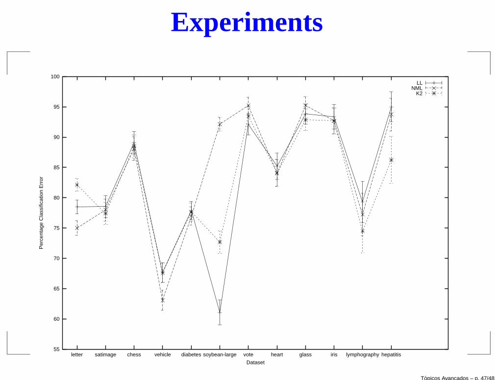
Experiments
55
60
65
70
75
80
85
90
95
100
hepatitislymphographyirisglassheartvotesoybean-largediabetesvehiclechesssatimageletter
Per
cent
age
Cla
ssifi
catio
n E
rror
Dataset
LLMDLNML
MIT(0.99)
Topicos Avancados – p. 46/48
Experiments
55
60
65
70
75
80
85
90
95
100
hepatitislymphographyirisglassheartvotesoybean-largediabetesvehiclechesssatimageletter
Per
cent
age
Cla
ssifi
catio
n E
rror
Dataset
LLNML
K2
Topicos Avancados – p. 47/48
Conclusions
The results show that Bayesian scores are hard to distinguish, performing well forlarge datasets.
The most impressive result was due to the NML score for the soybean-large dataset.
It seems that a good choice is to consider K2 for large datasets and NML for smallones.
Topicos Avancados – p. 48/48