screening prospects dominance transparencies for chapter 4
Post on 21-Dec-2015
219 views
TRANSCRIPT
Screening Prospects Dominance
• Transparencies for chapter 4

Introduction
In chapter 2 two types of dominance are introduced.
• Outcome dominance• Mean-variance dominance
Ask the students to recall them.
What role dominance plays?
Outcome Dominance
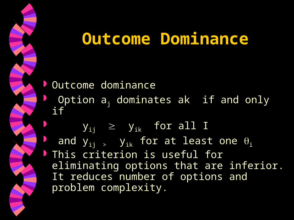
Outcome dominance Option aj dominates ak if and only if yij yik for all I and yij > yik for at least one i This criterion is useful for eliminating
options that are inferior. It reduces number of options and problem complexity.

Example for Outcome Dominance
Consider the following payoff matrix a1 a2 a3
1 6 3 8
2 5 4 2
3 7 6 3
a1 dominates a2
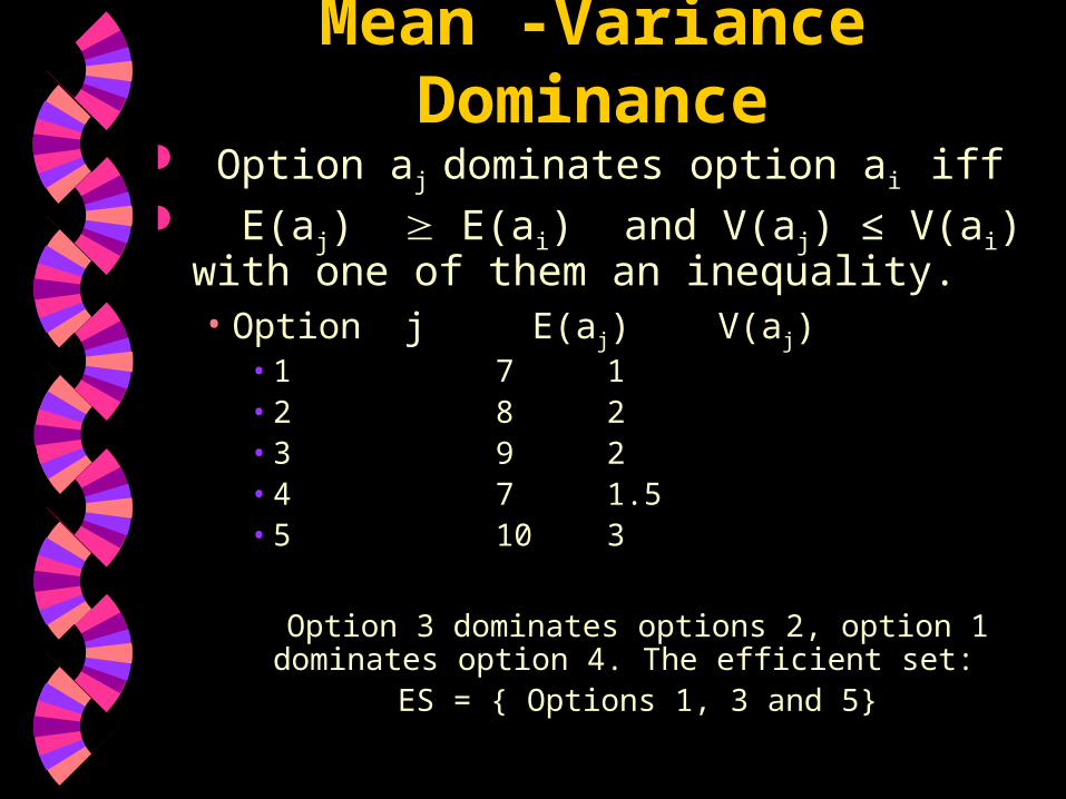
Mean -Variance Dominance Option aj dominates option ai iff E(aj) E(ai) and V(aj) ≤ V(ai) with one of
them an inequality.• Option j E(aj) V(aj)
• 1 7 1• 2 8 2• 3 9 2• 4 7
1.5• 5 10 3
Option 3 dominates options 2, option 1 dominates option 4. The efficient set:
ES = { Options 1, 3 and 5}

Mean -Variance Dominance Option aj dominates option ai iff E(aj) E(ai) and V(aj) ≤ V(ai) with one of
them an inequality.• Option j E(aj) V(aj)
• 1 7 1• 2 8 2• 3 9 2• 4 7
1.5• 5 10 3
Option 3 dominates options 2, option 1 dominates option 4. The efficient set:
ES = { Options 1, 3 and 5}
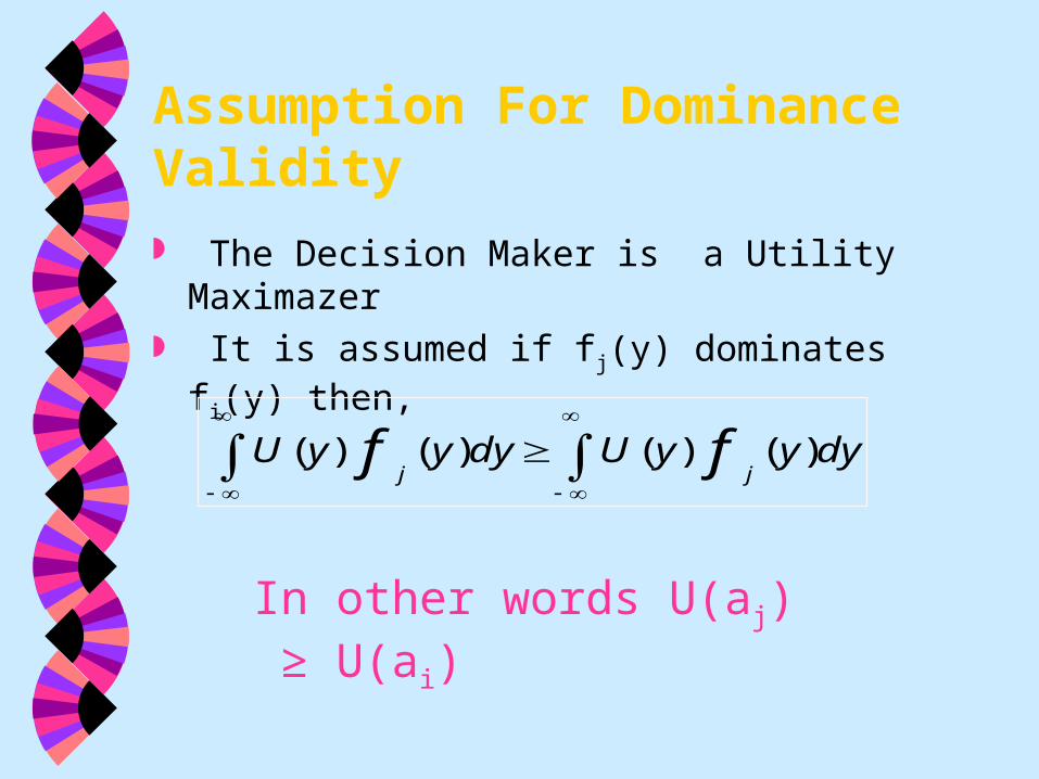
Assumption For Dominance Validity
The Decision Maker is a Utility Maximazer It is assumed if fj(y) dominates fi(y) then,
dyyyUdyyyU ffjj
)()()()(
In other words U(aj) ≥ U(ai)
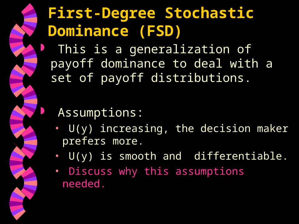
First-Degree Stochastic Dominance (FSD)
This is a generalization of payoff dominance to deal with a set of payoff distributions.
Assumptions:• U(y) increasing, the decision maker prefers
more. • U(y) is smooth and differentiable.• Discuss why this assumptions needed.

FSD Continued
aj dominates ai in FSD sense iff
Fi(y) Fi(y) y
Where F(y) is the cumulative probability distribution of the payoff.
In other words option j provides a higher chance of obtaining higher pay.

FSD Example 1
Check FSD for the following two course of actions
p( ) a1 a2
0.3
0.3
10 11
8 10
10 9
0.4
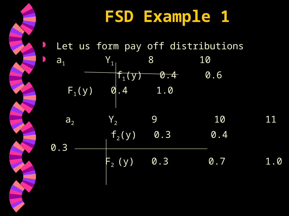
FSD Example 1
Let us form pay off distributions a1 Y1 8 10
f1(y) 0.4 0.6
F1(y) 0.4 1.0
a2 Y2 9 10 11
f2(y) 0.3 0.4 0.3
F2 (y) 0.3 0.7 1.0

Checking FSD Example1
Interval F1(y) Sign F2(y)
(-, 8) 0 = 0
[8, 9) 0.4 > 0
[9, 10) 0.4 > 0.3
[10, 11) 1.0 > 0.7
[11,) 1.0 = 1.0
F1(y) F2(y) , Therefore a1 dominates a2 in FSD
The above can be done graphically also.
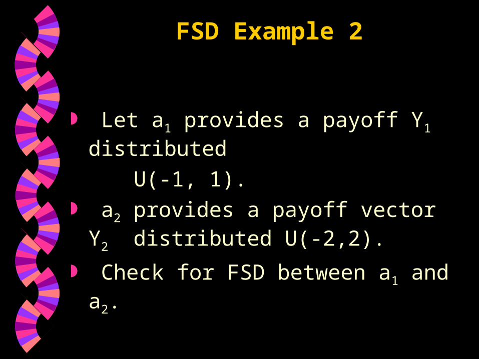
FSD Example 2
Let a1 provides a payoff Y1 distributed
U(-1, 1). a2 provides a payoff vector Y2 distributed
U(-2,2). Check for FSD between a1 and a2.
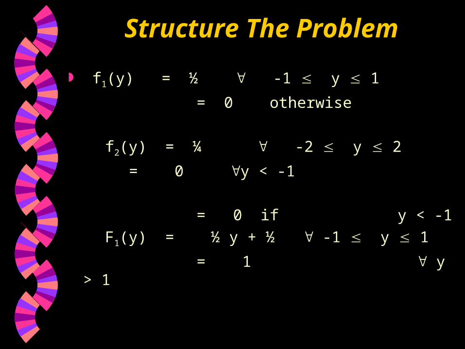
Structure The Problem
f1(y) = ½ -1 y 1
= 0 otherwise
f2(y) = ¼ -2 y 2
= 0 y < -1
= 0 if y < -1
F1(y) = ½ y + ½ -1 y 1
= 1 y > 1

FSD Example 2
= 0 y < -1
F2(y) = ¼ y + ½ -2 y 2
= 1 y > 2
It can be seen clearly that the two functions intersect at y=0
Therefore FSD fails or inconclusive.

Second-degree Stochastic Dominance (SSD)
Assumptions:• All FSD assumptions• Decision maker risk averse U(y)
concave. Let us define
•
aj dominates ai in SSD sense iff • Di(z) ≥ Dj(z) z
(y)dy(z)D f j
z
j
SSD
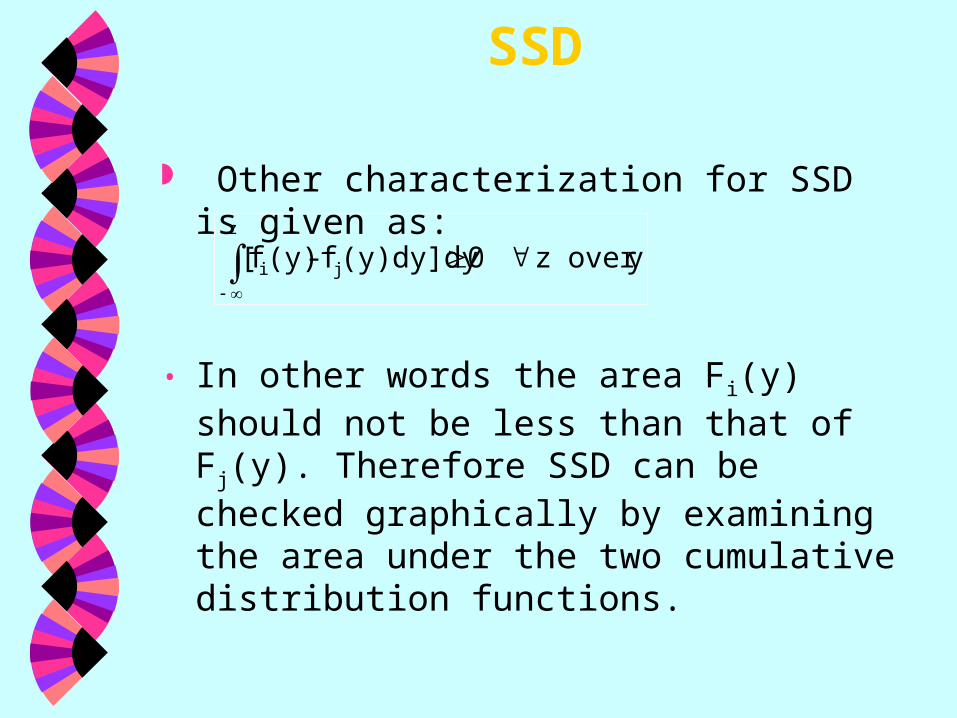
Other characterization for SSD is given as:
• In other words the area Fi(y) should not be less than that of Fj(y). Therefore SSD can be checked graphically by examining the area under the two cumulative distribution functions.
yover z 0 (y)dy]dy f - (y)f[ ji
z
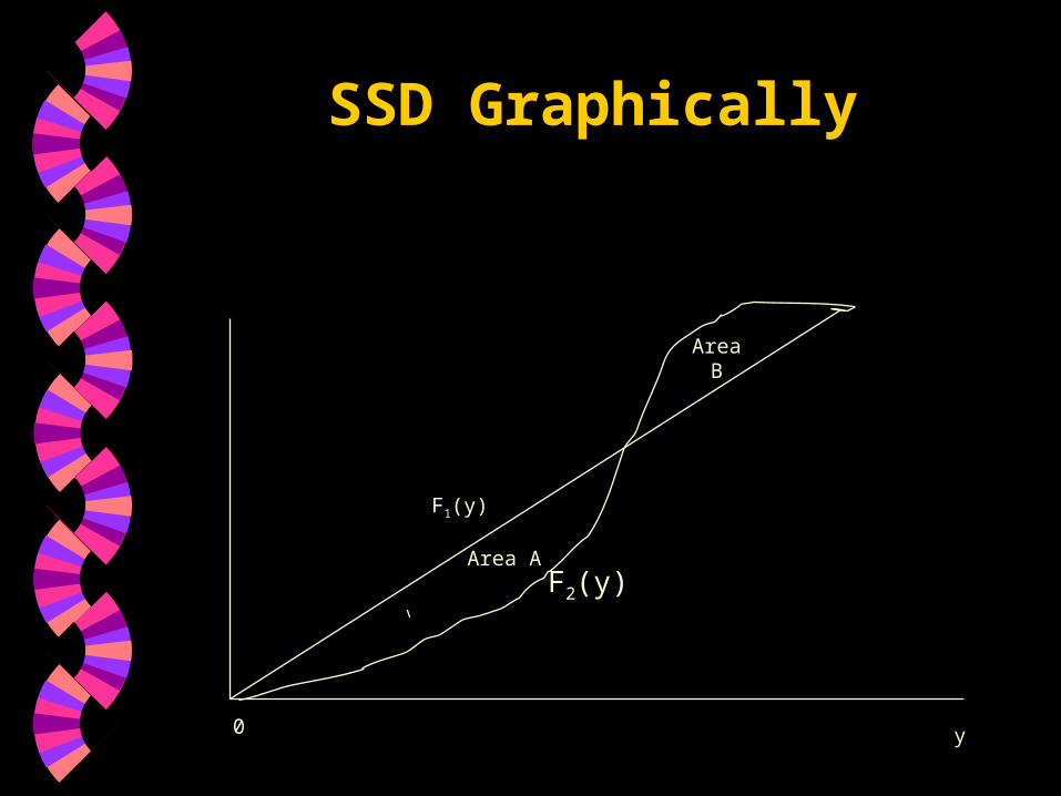
SSD Graphically
0 y
F1(y)
F2(y)Area A
Area B
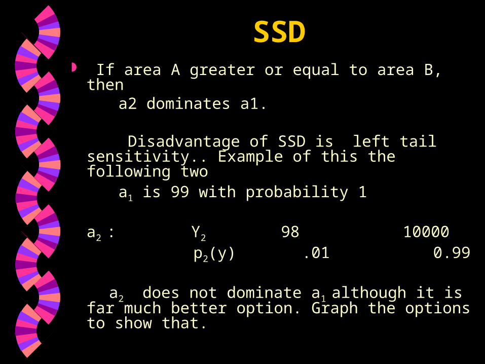
SSD If area A greater or equal to area B, then a2 dominates a1.
Disadvantage of SSD is left tail sensitivity.. Example of this the following two
a1 is 99 with probability 1
a2 : Y2 98 10000 p2(y) .01 0.99 a2 does not dominate a1 although it is far much
better option. Graph the options to show that.
SSD Example
Check SSD dominance for the case given in example 2 of FSD. Recall the case
a1 provides a payoff Y1 distributed
U(-1, 1). a2 provides a payoff vector Y2 distributed
U(-2,2). Check for SSD between a1 and a2.

SSD Example
= 0 if z <-1 D1(z) = ¼ z2 + ½ z + ¼ -1 z < 1
= z 1 z
= 0 z < -2
D2(z) = 1/8 z2 + ½ z + ½ -2 z < 2
= z
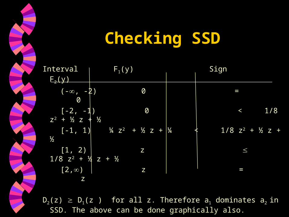
Checking SSD
Interval F1(y) Sign F2(y)
(-, -2) 0 = 0
[-2, -1) 0 < 1/8 z2 + ½ z + ½
[-1, 1) ¼ z2 + ½ z + ¼ < 1/8 z2 + ½ z + ½
[1, 2) z 1/8 z2 + ½ z + ½
[2,) z = z
D2(z) D1(z ) for all z. Therefore a1 dominates a2 in SSD. The above can be done graphically also.
Some Results
If FSD holds then SSD holds. Proof is obvious.
If SSD holds FSD may not hold. The previous example shows that FSD does not but SSD holds.

Third Stochastic Dominance (TSD)
Assumptions:• All the assumptions of SSD
• Decision maker decreasing risk averse
• How to check decreasing risk averse
Define the following:
Where D(z) as defined for SSD
D(z)dz(t)TDt
j
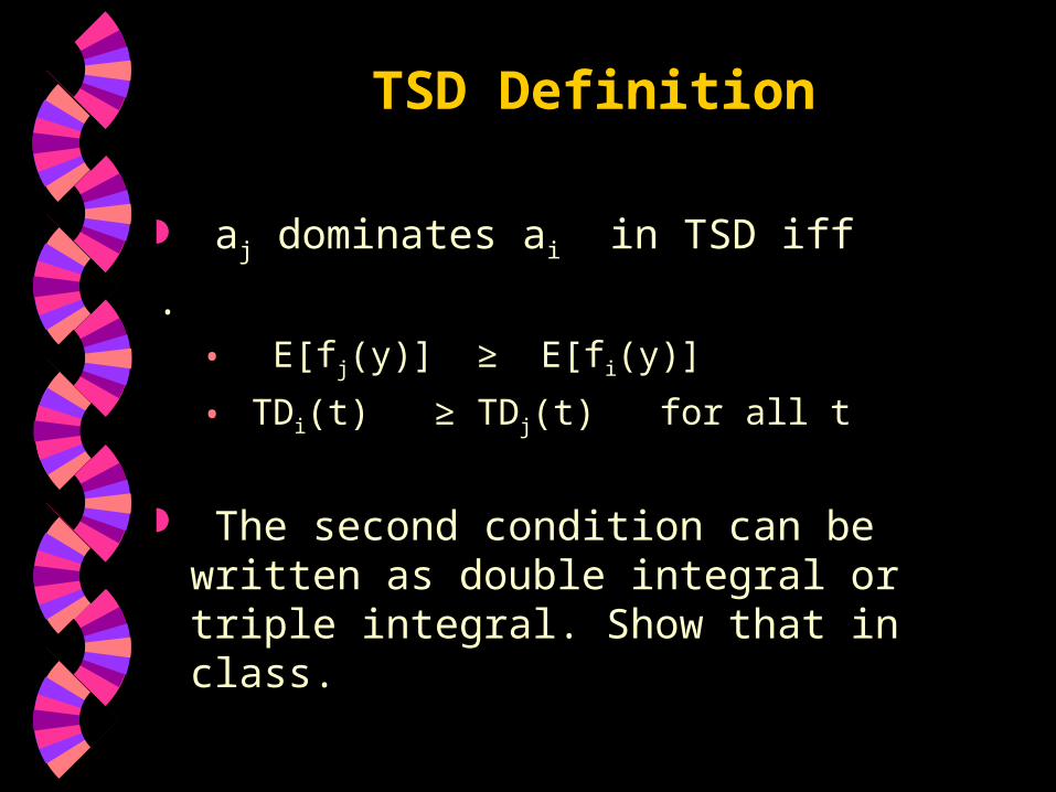
TSD Definition
aj dominates ai in TSD iff
. • E[fj(y)] ≥ E[fi(y)]
• TDi(t) ≥ TDj(t) for all t
The second condition can be written as double integral or triple integral. Show that in class.
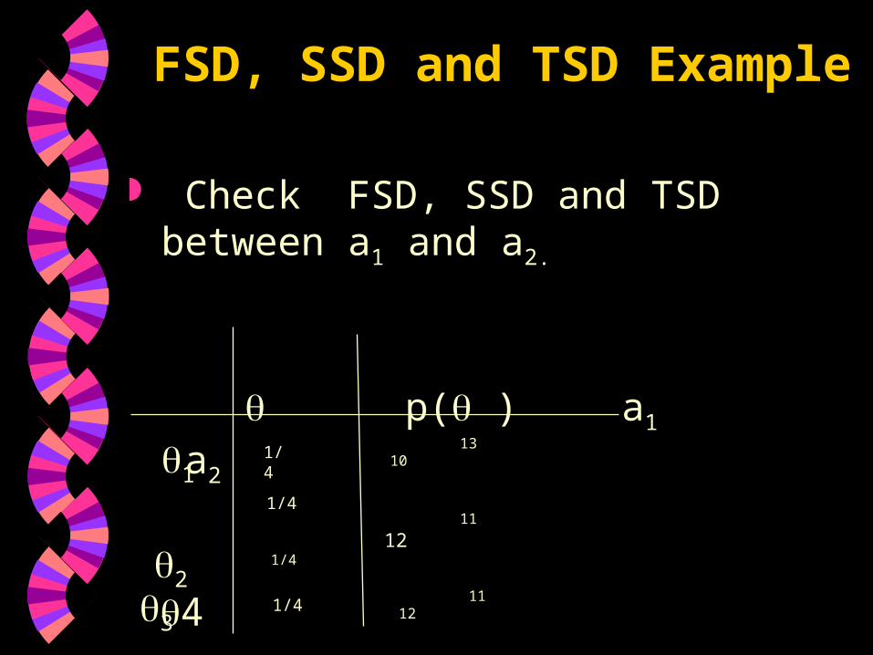
FSD, SSD and TSD Example
Check FSD, SSD and TSD between a1 and a2.
p( ) a1 a2 1
2
3
1/4
1/4
13 10
11 12
11 12
11 12
1/4
4 1/4
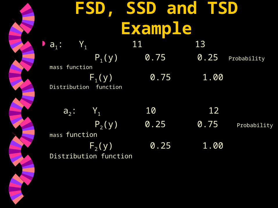
FSD, SSD and TSD Example
a1: Y1 11 13
P1(y) 0.75 0.25 Probability mass function
F1(y) 0.75 1.00 Distribution function
a2: Y1 10 12
P2(y) 0.25 0.75 Probability mass function
F2(y) 0.25 1.00 Distribution function
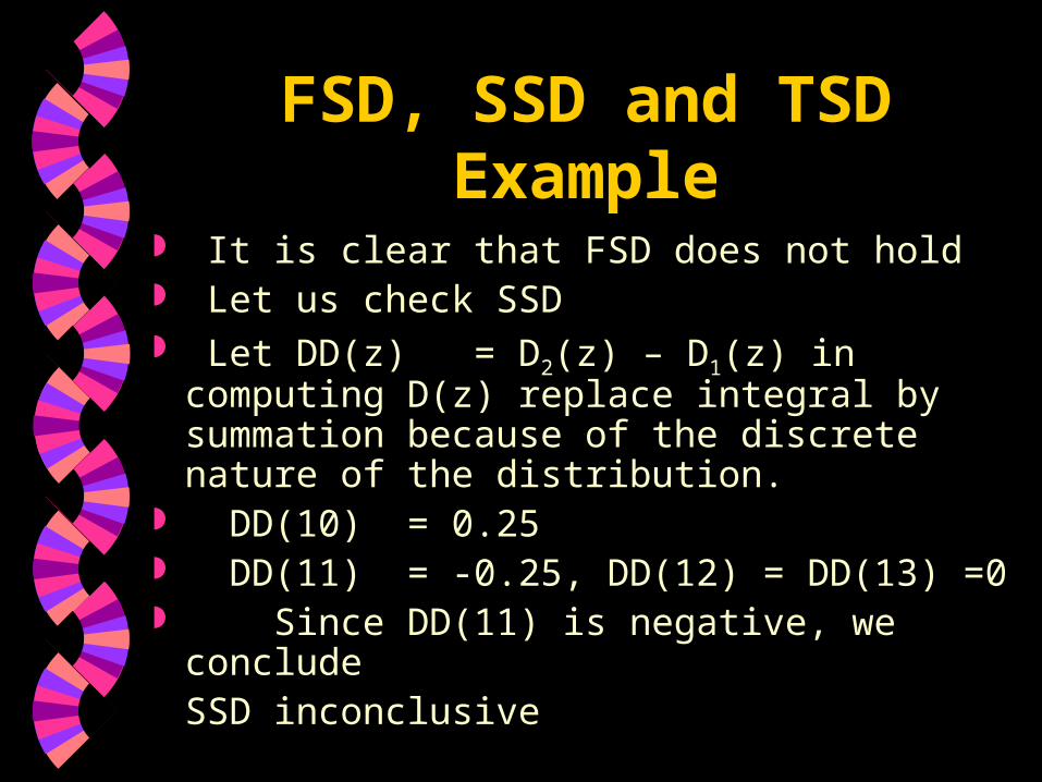
FSD, SSD and TSD Example
It is clear that FSD does not hold Let us check SSD Let DD(z) = D2(z) – D1(z) in computing
D(z) replace integral by summation because of the discrete nature of the distribution.
DD(10) = 0.25 DD(11) = -0.25, DD(12) = DD(13) =0 Since DD(11) is negative, we conclude
SSD inconclusive

FSD, SSD and TSD Example
Alternative way for checking SSD Interval D1(z) sign D2(z)
(- , 10) 0 = 0
[10, 11) 0 < 0.25z – 2.5
[11, 12) 0.75 z – 8.25 < & > 0.25 z – 2.5
[12, 13) 0.75 z – 8.25 z - 11.5
[13, ) z – 11.5 = z – 11.5
SSD inconclusive

TSD
To show TSD hold we need to show that
0)(
zDDt
for t = 10, 11, 12, 13
It can be seen that the sum for the above formula at t = 10 is 0.25 , at t=11 it is 0 and it stays 0 for all other values.
Also E(a1) = E(a2) = 11.5
Therefore TSD holds and a1 dominates a2

Nth Stochastic Dominance(NSD)
NSD can similarly be defined by integrating Fi(y) and Fj(y) n-1 times and examining the difference between the two integrals. If it has the same sign, then dominance holds, otherwise it does not.
IF FSD holds then NSD holds.

Applied Example in Securities
Porter and Carey (1974) applied stochastic dominance to screen 16 randomly selected companies. The companies are:
Company Number Company Name
1 Federal Paper Board 2 American Machine and Foundry
3 Smith Kline/French Lab 4 Rayonier 5 American Tobacco 6 Crowell-Collier 7 American Seating 8 Emerson Electric 9 Riegel Textile 10 Cero 11 American Distilling 12 American Investment 13 Johnson and Johnson 14 United Aircraft 15 Dresser Industries 16 Schering

Case Analysis
The rate of retain (ROR) for 54 periods (quarter) from the last quarter of 1963 to the first quarter of 1968. The distribution of the rate of return was developed.
RORt = (Pt – Pt-1) + Dt)/Pt-1
Pt = price at period t
Dt = Dividend in period t

Case Analysis Using FSD
The results of FSD is Company 2 dominates 3
Company 5 dominates 3
Company 8 dominates 3, 5, 7

Case Analysis Using SSD
Results of SSD Dominance test Company 2 dominated 3
Company 4 dominated 10Company 5 dominated 1,2,3,7.Company 7 dominated 1Company 8 dominated 1,2,3,4,5,6,7,9,10,11,13,14
15Company 9 dominated 10Company 11 dominated 3Company 12 dominated 3, 11Company 13 dominated 1, 10Company 14 dominated 10Company 15 dominated 6, 9, 10, 14Company 16 dominated 1, 4, 6, 9, 10, 13, 14, 15
Companies 1, 3, 6, 10 dominated none
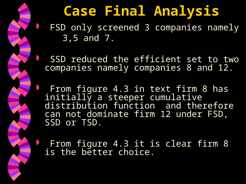
Case Final Analysis FSD only screened 3 companies namely 3,5 and 7.
SSD reduced the efficient set to two companies namely companies 8 and 12.
From figure 4.3 in text firm 8 has initially a steeper cumulative distribution function and therefore can not dominate firm 12 under FSD, SSD or TSD.
From figure 4.3 it is clear firm 8 is the better choice.
Comments on Screening
Screening by dominance usually reduces the number of options to a manageable size.
In some cases screening by dominance could leave two options that may be ranked first and last when maximizing expected utility.
Assign example on page 77 for discussion by students