lable at ScienceDirect

Physics and Chemistry of the Earth 94 (2016) 155e166

Contents lists avai

Physics and Chemistry of the Earth

journal homepage: www.elsevier .com/locate/pce

Seasonal drought predictability in Portugal usingstatisticaledynamical techniques

A.F.S. Ribeiro, C.A.L. Pires*

Instituto Dom Luiz (IDL), Faculdade de Ciencias, Universidade de Lisboa, 1749-016 Lisboa, Portugal

a r t i c l e i n f o

Article history:Received 10 December 2014Received in revised form18 March 2015Accepted 23 April 2015Available online 16 May 2015

Keywords:Long-range forecastsPredictabilityStatistical predictionDrought index SPIPrecipitation forecasting

* Corresponding author.E-mail address: clpires@fc.ul.pt (C.A.L. Pires).

http://dx.doi.org/10.1016/j.pce.2015.04.0031474-7065/© 2015 Elsevier Ltd. All rights reserved.

a b s t r a c t

Atmospheric forecasting and predictability are important to promote adaption and mitigation measuresin order to minimize drought impacts. This study estimates hybrid (statisticaledynamical) long-rangeforecasts of the regional drought index SPI (3-months) over homogeneous regions from mainlandPortugal, based on forecasts from the UKMO operational forecasting system, with lead-times up to6 months. ERA-Interim reanalysis data is used for the purpose of building a set of SPI predictors inte-grating recent past information prior to the forecast launching. Then, the advantage of combining pre-dictors with both dynamical and statistical background in the prediction of drought conditions atdifferent lags is evaluated. A two-step hybridization procedure is performed, in which both forecastedand observed 500 hPa geopotential height fields are subjected to a PCA in order to use forecasted PCs andpersistent PCs as predictors. A second hybridization step consists on a statistical/hybrid downscaling tothe regional SPI, based on regression techniques, after the pre-selection of the statistically significantpredictors. The SPI forecasts and the added value of combining dynamical and statistical methods areevaluated in cross-validation mode, using the R2 and binary event scores. Results are obtained for thefour seasons and it was found that winter is the most predictable season, and that most of the predictivepower is on the large-scale fields from past observations. The hybridization improves the downscalingbased on the forecasted PCs, since they provide complementary information (though modest) beyondthat of persistent PCs. These findings provide clues about the predictability of the SPI, particularly inPortugal, and may contribute to the predictability of crops yields and to some guidance on users (such asfarmers) decision making process.

© 2015 Elsevier Ltd. All rights reserved.

1. Introduction

Drought episodes in the Iberian Peninsula (IP) have becomemore frequent and severe (Vicente-Serrano et al., 2014; Sousa et al.,2011), causing several consequences on the socioeconomic andecological sectors, and leading to major impacts on vegetation(Vicente-Serrano et al., 2013; Gouveia et al., 2012, 2009; Vicente-Serrano, 2007). Extreme episodes, such as the recent 2011e2012,2004e2005 droughts at Iberia (Trigo et al., 2013; García-Herreraet al., 2007) and the heatwave of 2003 in Europe (Trigo et al.,2005) can seriously affect the agricultural and the hydrologic ac-tivities, conditioning the crops and, consequently, requiring adap-tation and mitigation measures often entailing high costs. Atendency towards a drier Mediterranean during the 21st century

(Giorgi and Lionello, 2008) and the strong variability of the pre-cipitation regime in the IP (Esteban-Parra et al., 1998) enhance theoccurrence of droughts and promote the need for drought forecast(either seasonal and climatic), in order to prevent the mentionedimpacts.

The predictability of the atmospheric seasonal variability (e.g.Brankovic et al., 1994; e.g. Van den Dool, 1994) has many potentialapplications, in particular those related to risk management due todrought conditions. Predictions on seasonal time-scales rely on thelow-frequency variability of the atmosphere, since themajor part ofthe atmospheric variability show variations on long time scales(seasons and years), which can be predictable to some extent. Oneof the most important of these low-frequency modes in Europe isthe North Atlantic Oscillation (NAO), the dominant mode of winterclimate variability over the North Atlantic-European (NAE) region(e.g. Hurrel, 1995), which plays the most important role in precip-itation variability over Iberia (Trigo et al., 2004; Rodríguez-Pueblaet al., 2001; Pires and Perdig~ao, 2007). Nevertheless, despite the

A.F.S. Ribeiro, C.A.L. Pires / Physics and Chemistry of the Earth 94 (2016) 155e166156

much lower forecast skill over extratropics than in tropical regions(e.g. Rowell, 1998; Zhu et al., 2014) it is not negligible, and large-scale features has long been regarded as more predictable thansmall scales (Van den Dool and Saha, 1990). In a simple way, low-frequency modes can be interpreted as sources of predictabilityor “windows of opportunity” of potential predictability: the abilityto predict well the low-frequency modes, may lead to a good pre-diction of the regional features, such as droughts.

Long-range forecasts in Europe have been carried out by manyoperational meteorological centers, such as the European Center forMedium-Range Weather Forecast (ECMWF), the UK Met Office(UKMO) and the M�et�eo-France. Dynamical predictions systems arewidely used for long-range forecasts (e.g. Doblas-Reyes et al., 2009;Vitart et al., 2007), as well as statistical approaches (e.g. Follandet al., 2012; Morid et al., 2007). Given the availability of produc-ing forecasts based on both dynamical and statistical systems, thehybrid combination of statistical and dynamical methods emergedas a commonly and useful approach for long-range forecasts inorder to take advantage of both approaches using, for instance:probabilistic forecasting based on Gaussian distribution anddeterministic forecasting (D�equ�e and Stroe, 1994), Bayesian jointprobability (BJP) (Peng et al., 2014), spaceetime principal compo-nents (ST-PCs) (Vautard et al., 1996; Sarda et al., 1996) e obtainedfrom the Multi-Singular Spectrum Analysis (MSSA) e regression-based models (Kim and Webster, 2010), and Maximum Covari-ance Analysis (MCA) (Coelho et al., 2006).

A hybrid approach that has been followed relies in a two-stepprocedure, in which the predictors are first numerically fore-casted and then statistically processed, and finally used to empir-ically estimate the predict and (e.g. Pires, 1996; Sarda et al., 1996).Recently, using the most recent seasonal Integrated Forecast Sys-tems (IFS) from the EMCWF, Vitart (2014) have shown that the skillof the NAO monthly forecasts have been improving, which isparticularly interesting given the importance of this index for theprecipitation variability over the NAE region. One of the goals ofthis work is to take advantage of the skill of the dynamical modelsin forecasting the low-frequency modes (Peng et al., 2014; Kimet al., 2012), using the first leading Principal Components (PCs) ofdynamical seasonal forecasts of the geopotential at 500 hPa (first-step of the hybrid procedure), and then perform a statisticaldownscaling of those predictors to the regional scale, based onregression techniques (second-step of the hybrid procedure). Thefirst-step of the hybrid procedure also includes the PCs of prior(forecasting initialization date) observations of geopotential, gath-ering a pool of predictors from both dynamical and statisticalbackgrounds. The influence of each predictor is here assessed, andthe added value of hybridizing dynamical and statistical basedpredictors is evaluated.

Besides the NAO, evidence is found that other main low-frequency modes are linked to the precipitation regime over IP,which is marked by a strong variability enhance the occurrence ofdroughts (Esteban-Parra et al., 1998), for instance: the ScandinavianPattern (SCAND) and the East-Atlantic pattern (EA) (e.g. Rodriguez-Puebla et al., 1998); the East-Atlantic/West Russian Pattern (EA/WR) (Vicente-Serrano and L�opez-Moreno, 2006); which suggestspossible drought predictive skills of these teleconnection patterns.Another source of predictability is the influence, though weaker, ofthe El Ni~noeSouthern Oscillation phenomenon (ENSO) on precip-itation (e.g. deCastro et al., 2006; Vicente-Serrano, 2005; Pozo-V�azquez et al., 2001; Rodriguez-Puebla et al., 1998).

An important tool when analyzing drought conditions are thedrought indices, which allows for the assignment of different de-grees of intensity, duration and spatial extent of droughts. Vicente-Serrano (2005) has discussed the influence of El Ni~no and La Ni~naevents on droughts in the IP using the Standardized Precipitation

Index (SPI), developed by McKee et al. (1993), which is based on aprobabilistic approach of the precipitation. Another widelyemployed drought index is the Palmer Drought Severity Index(PDSI), developed by Palmer (1965) which, besides precipitation, isbased on the soil water budget. More recently, Vicente-Serranoet al. (2010) has formulated an index that seeks the combined in-fluence of precipitation and evapotranspiration: the StandardizedPrecipitation Evaporation Index (SPEI).

The present work aims to contribute to the assessment andimprovement of the seasonal predictability of the SPI at a time scaleof 3-months (predictand) in the mainland Portugal (western Ibe-ria), with lead-times up to 6 months, based on hybridizationtechniques. Coelho et al. (2006) has developed a single integratedforecast of seasonal of rainfall that gathers prediction informationfrom three dynamical systems and an empirical model. Morerecently, Coelho and Costa (2010) discusses the challenges ofintegrating seasonal forecasts to help the end user managing pro-cess. Similarly, the present study also intends to contribute to animproved understanding of the relevance of combining dynamicaland statistical techniques in the prediction of droughts over thePortuguese territory, in order to provide some guidance on users(such as farmers) decision making process.

In Section 2 the data and the applied methodology is described,focusing on the two-step hybridization procedure, the selection ofthe best predictors and the formulation of the statistical down-scaling. In Section 3 the results of the forecasts (statistical andhybrid) of the drought index are evaluated according to the lead-time, season and region. A discussion and conclusions follow inSection 4.

2. Data and methods description

2.1. Regional drought index

In this study the Standard Precipitation Index (SPI) is computedbased on monthly precipitation time series, providing a measure ofanomalies in precipitation (McKee et al., 1993). In order to considerhomogeneous climate regions for the computation of regional SPItime-series, the recent high-resolution (0.2� � 0.2�) gridded data-set PT02 developed by Belo-Pereira et al. (2011) is considered. Thisnew dataset based on a dense network of observed data overPortugal (several hundred stations) is a rather good representationof the precipitation regime over Portugal, resulting from theinterpolation of observations using the ordinary kriging method,after quality control and homogenization steps.

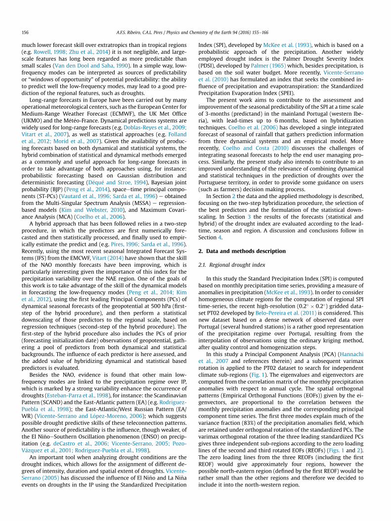
In this study a Principal Component Analysis (PCA) (Hannachiet al., 2007 and references therein) and a subsequent varimaxrotation is applied to the PT02 dataset to search for independentclimate sub-regions (Fig. 1). The eigenvalues and eigenvectors arecomputed from the correlation matrix of the monthly precipitationanomalies with respect to annual cycle. The spatial orthogonalpatterns (Empirical Orthogonal Functions (EOFs)) given by the ei-genvectors, are proportional to the correlation between themonthly precipitation anomalies and the corresponding principalcomponent time series. The first three modes explain much of thevariance fraction (83%) of the precipitation anomalies field, whichare retained under orthogonal rotation of the standardized PCs. Thevarimax orthogonal rotation of the three leading standardized PCsgives three independent sub-regions according to the zero loadinglines of the second and third rotated EOFs (REOFs) (Figs. 1 and 2).The zero loading lines from the three REOFs (including the firstREOF) would give approximately four regions, however thepossible north-eastern region (defined by the first REOF) would berather small than the other regions and therefore we decided toinclude it into the north-western region.

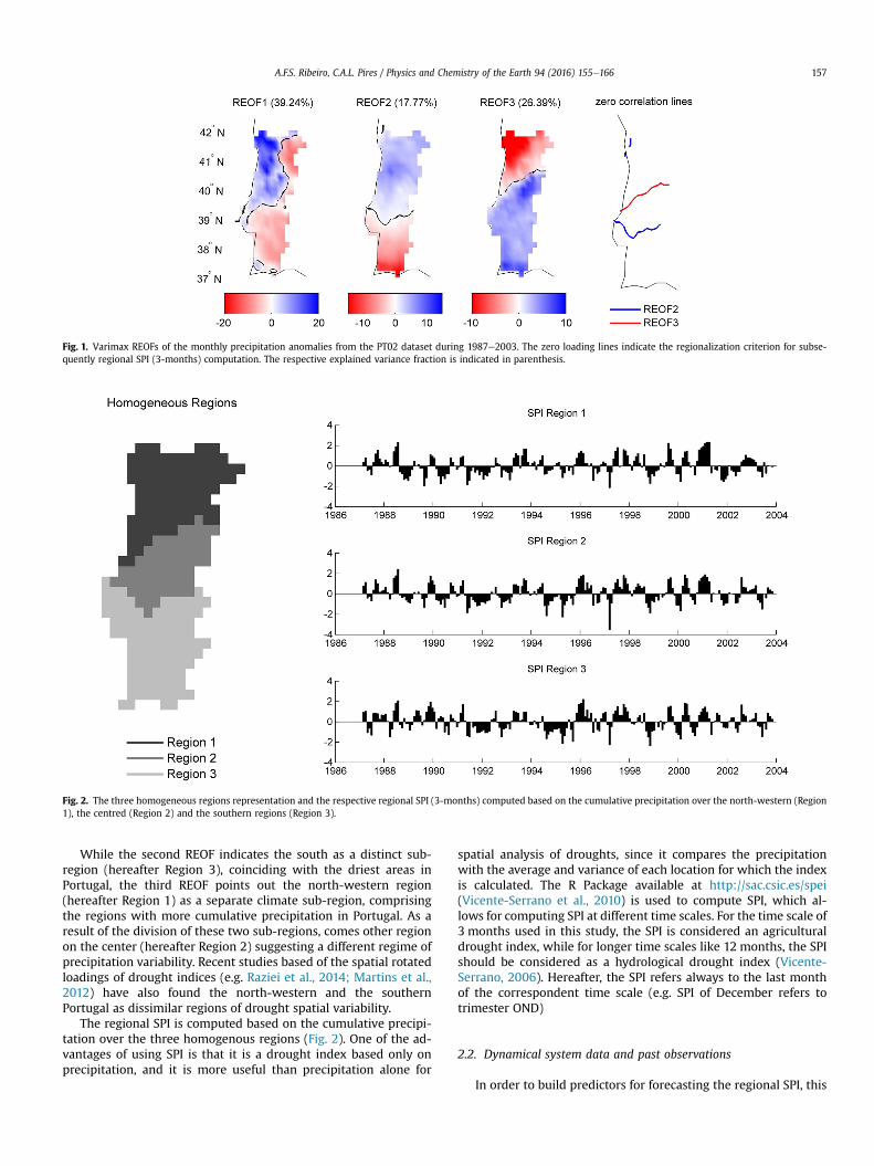
Fig. 1. Varimax REOFs of the monthly precipitation anomalies from the PT02 dataset during 1987e2003. The zero loading lines indicate the regionalization criterion for subse-quently regional SPI (3-months) computation. The respective explained variance fraction is indicated in parenthesis.

Fig. 2. The three homogeneous regions representation and the respective regional SPI (3-months) computed based on the cumulative precipitation over the north-western (Region1), the centred (Region 2) and the southern regions (Region 3).

A.F.S. Ribeiro, C.A.L. Pires / Physics and Chemistry of the Earth 94 (2016) 155e166 157

While the second REOF indicates the south as a distinct sub-region (hereafter Region 3), coinciding with the driest areas inPortugal, the third REOF points out the north-western region(hereafter Region 1) as a separate climate sub-region, comprisingthe regions with more cumulative precipitation in Portugal. As aresult of the division of these two sub-regions, comes other regionon the center (hereafter Region 2) suggesting a different regime ofprecipitation variability. Recent studies based of the spatial rotatedloadings of drought indices (e.g. Raziei et al., 2014; Martins et al.,2012) have also found the north-western and the southernPortugal as dissimilar regions of drought spatial variability.

The regional SPI is computed based on the cumulative precipi-tation over the three homogenous regions (Fig. 2). One of the ad-vantages of using SPI is that it is a drought index based only onprecipitation, and it is more useful than precipitation alone for

spatial analysis of droughts, since it compares the precipitationwith the average and variance of each location for which the indexis calculated. The R Package available at http://sac.csic.es/spei(Vicente-Serrano et al., 2010) is used to compute SPI, which al-lows for computing SPI at different time scales. For the time scale of3 months used in this study, the SPI is considered an agriculturaldrought index, while for longer time scales like 12 months, the SPIshould be considered as a hydrological drought index (Vicente-Serrano, 2006). Hereafter, the SPI refers always to the last monthof the correspondent time scale (e.g. SPI of December refers totrimester OND)

2.2. Dynamical system data and past observations

In order to build predictors for forecasting the regional SPI, this

A.F.S. Ribeiro, C.A.L. Pires / Physics and Chemistry of the Earth 94 (2016) 155e166158

study uses monthly means of geopotential height at 500 hPa(hereafter referred as z500) from the UKMO forecasting system(ECMWF data arquive), which provides ensemble means (monthlymeans averaged over all the ensemble members) since 1987 withlead-times up to 6 months, to be used here.

Monthly ERA-Interim reanalysis of the z500 field from theforecasting initialization date is considered for the purpose of buildSPI predictors integrating recent past information prior to theforecast launching. For example, a 1 month lead forecast for the SPIof December is initialized on 1 November, whereas 2 month leadforecast for December is initialized on 1 October. For eachDecember forecast, we use here 6 prior corresponding reanalysisvalues, covering the forecast lead-times from 1 to 6 months. ERA-Interim reanalysis uses input observations, so reanalysis data isconsidered as past observations, since it corresponds to what isknown before the forecast. The common period 1987e2003(16 years) between the data from the UKMO forecasting system andthe PT02 is used for all data sets considered in this study.

2.3. Two-step hybridization procedure

This study estimates hybrid (statisticaledynamical) predictionsof the regional drought index SPI. A key concept of the presentmethodology is the concept of hybridization, here considered as thecombination of predictors of different kinds: the dynamical fore-casts and the past observations. A two-step hybridization proced-ure is adopted: the first-step concerns the application of PCA to theoutput dynamical forecasting system and also to past observations,in order to build the pool of predictors (PCs) from both dynamicaland statistical backgrounds. The second-step regards the statisticaldownscaling of the predictors, taking the SPI as the predictand,

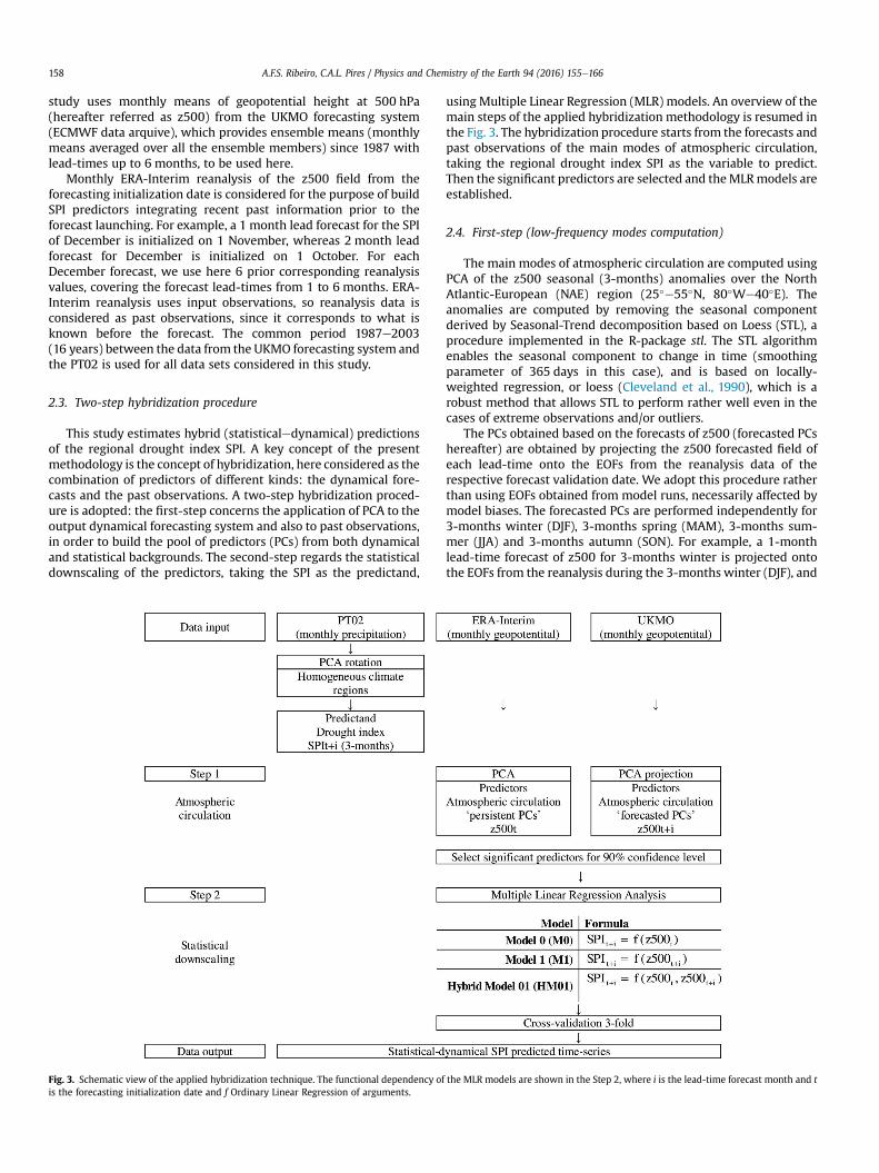
Fig. 3. Schematic view of the applied hybridization technique. The functional dependency ofis the forecasting initialization date and f Ordinary Linear Regression of arguments.

using Multiple Linear Regression (MLR) models. An overview of themain steps of the applied hybridization methodology is resumed inthe Fig. 3. The hybridization procedure starts from the forecasts andpast observations of the main modes of atmospheric circulation,taking the regional drought index SPI as the variable to predict.Then the significant predictors are selected and theMLRmodels areestablished.

2.4. First-step (low-frequency modes computation)

The main modes of atmospheric circulation are computed usingPCA of the z500 seasonal (3-months) anomalies over the NorthAtlantic-European (NAE) region (25�e55�N, 80�We40�E). Theanomalies are computed by removing the seasonal componentderived by Seasonal-Trend decomposition based on Loess (STL), aprocedure implemented in the R-package stl. The STL algorithmenables the seasonal component to change in time (smoothingparameter of 365 days in this case), and is based on locally-weighted regression, or loess (Cleveland et al., 1990), which is arobust method that allows STL to perform rather well even in thecases of extreme observations and/or outliers.

The PCs obtained based on the forecasts of z500 (forecasted PCshereafter) are obtained by projecting the z500 forecasted field ofeach lead-time onto the EOFs from the reanalysis data of therespective forecast validation date. We adopt this procedure ratherthan using EOFs obtained from model runs, necessarily affected bymodel biases. The forecasted PCs are performed independently for3-months winter (DJF), 3-months spring (MAM), 3-months sum-mer (JJA) and 3-months autumn (SON). For example, a 1-monthlead-time forecast of z500 for 3-months winter is projected ontothe EOFs from the reanalysis during the 3-months winter (DJF), and

the MLR models are shown in the Step 2, where i is the lead-time forecast month and t

A.F.S. Ribeiro, C.A.L. Pires / Physics and Chemistry of the Earth 94 (2016) 155e166 159

a 2-month lead-time forecast of z500 for 3-months spring areprojected onto the EOFs from the reanalysis during the 3-monthsspring (MAM).

For each lead-time, a benchmark empirical PC is given by the‘persistence’, i.e. the observed PCs at the date of initialization of theforecast (persistent PCs hereafter). For example, to the 1-monthlead-time forecasted PCs of DJF, it corresponds the persistent PCsbased on the reanalysis of NDJ.

Based on the examination of the number of PCs (forecasted andpersistent) that explain approximately over 50% of the z500 totalvariance (explained variance depends on the season and on thelead-time that is considered), the first four persistent PCs and thefirst four forecasted PCs are retained. Those variance-leading PCshave in general a large-scale and low-frequency signature leadingto some potential predictability.

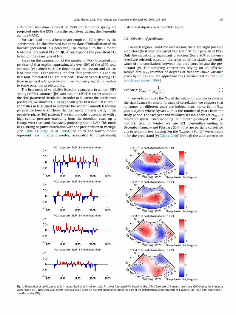
The first mode of variability based on reanalysis in winter (DJF),spring (MAM), summer (JJA) and autumn (SON) is rather similar tothe NAO pattern of circulation. In order to illustrate the persistencepredictors, we show in Fig. 4 (right panel) the first four EOFs of z500anomalies in NDJ (used to compute the winter 1-month lead-timepersistence forecasts). There, the first mode projects partly in thenegative-phase NAO pattern. The second mode is associated with ahigh central pressure extending from the American coast up toEuropewest coast and also partly projecting on the NAO. This modehas a strong negative correlation with the precipitation in Portugal(see Table 1) (Trigo et al., 2004).The third and fourth modesrepresent less important modes, associated to longitudinally

Fig. 4. Illustration of predictors used in 1-month lead-time in winter. Left: First four forecaswinter (DJF), i.e. 3 times per year. Right: First four EOFs, based on the past observations frommonths winter (NDJ).

distributed dipoles over the NAE region.

2.5. Selection of predictors

For each region, lead-time and season, there are eight possiblepredictors (first four forecasted PCs and first four persistent PCs).Only the statistically significant predictors (for a 90% confidencelevel) are selected, based on the criterion of the statistical signifi-cance of the correlations between the predictors (x) and the pre-dictand (y). The sampling correlations relying on an effectivesample size Ness (number of degrees of freedom) have variancegiven by Eq. (1) and are approximately Gaussian distributed (vonStorch and Zwiers, 1999).

var½corðx; yÞNess� ¼ 1

Ness � 3(1)

In order to compute the Ness of the validation sample to enter inthe significance threshold formula of correlation, we suppose thatoutcomes on different years are independent, hence Ness ¼ Ness/year � Nyears where Nyears ¼ 16 is the number of years from thestudy period. For each year and validated season, there are Nrea ¼ 3realizations/year corresponding to monthly-delayed SPI (3-months) (e.g. in winter we use SPI (3-months) ending inDecember, January and February (DJF)) that are partially correlateddue to temporal overlapping. For the Ness/year (Eq. (2)) we estimateit for the predictand (y) (Zieba, 2010) through the auto-correlation

ted PCs based on the UKMO forecasts of 1-month lead-time z500 during the 3-monthsthe date of the initialization of the forecasts of 1-month lead-time z500 during the 3-

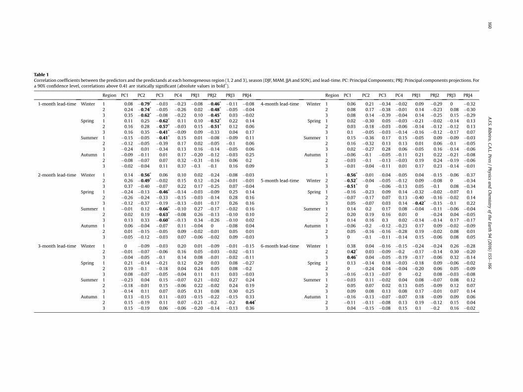
Table 1Correlation coefficients between the predictors and the predictands at each homogeneous region (1, 2 and 3), season (DJF, MAM. JJA and SON), and lead-time. PC: Principal Components; PRJ: Principal components projections. Fora 90% confidence level, correlations above 0.41 are statically significant (absolute values in bold*).

Region PC1 PC2 PC3 PC4 PRJ1 PRJ2 PRJ3 PRJ4 Region PC1 PC2 PC3 PC4 PRJ1 PRJ2 PRJ3 PRJ4

1-month lead-time Winter 1 0.08 �0.79* �0.03 �0.23 �0.08 �0.46* �0.11 �0.08 4-month lead-time Winter 1 0.06 0.21 �0.34 �0.02 0.09 �0.29 0 �0.322 0.24 �0.74* �0.05 �0.26 0.02 �0.48* �0.05 �0.04 2 0.08 0.17 �0.38 �0.01 0.14 �0.23 0.08 �0.303 0.35 �0.62* �0.08 �0.22 0.10 �0.45* 0.03 �0.02 3 0.08 0.14 �0.39 �0.04 0.14 �0.25 0.15 �0.29

Spring 1 0.11 0.25 �0.62* 0.11 0.10 �0.52* 0.22 0.14 Spring 1 0.02 �0.30 0.05 �0.03 �0.21 �0.02 �0.14 0.132 0.16 0.28 �0.57* �0.03 0.15 �0.51* 0.12 0.06 2 0.03 �0.18 �0.03 �0.06 �0.14 �0.12 �0.12 0.133 0.16 0.35 �0.41* �0.09 0.09 �0.33 0.04 0.17 3 0.1 �0.05 �0.03 �0.14 �0.16 �0.12 �0.17 0.07

Summer 1 �0.15 �0.05 �0.41* 0.15 0.01 �0.08 �0.09 0.11 Summer 1 0.15 �0.36 0.17 0.15 �0.05 0.09 �0.09 �0.032 �0.12 �0.05 �0.39 0.17 0.02 �0.05 �0.1 0.06 2 0.16 �0.32 0.13 0.13 0.01 0.06 �0.1 �0.053 �0.24 0.01 �0.34 0.13 0.16 �0.14 �0.05 0.06 3 0.02 �0.27 0.28 0.06 �0.05 0.16 �0.14 �0.06

Autumn 1 �0.09 �0.11 0.01 0.17 �0.20 �0.12 �0.03 0.25 Autumn 1 �0.06 �0.1 �0.05 �0.11 0.21 0.22 �0.21 �0.082 �0.08 �0.07 0.07 0.32 �0.31 �0.16 0.06 0.2 2 �0.03 �0.1 �0.13 �0.03 0.19 0.24 �0.19 �0.063 �0.02 �0.04 0.11 0.37 �0.3 �0.1 0.16 0.09 3 �0.01 �0.04 �0.11 0.01 0.17 0.23 �0.14 �0.01

2-month lead-time Winter 1 0.14 �0.56* 0.06 0.10 0.02 �0.24 �0.08 �0.03 1 �0.56* �0.01 �0.04 �0.05 0.04 �0.15 �0.06 �0.372 0.26 �0.49* �0.02 0.15 0.12 �0.24 �0.01 �0.01 5-month lead-time Winter 2 �0.52* �0.04 �0.05 �0.12 0.09 �0.08 0 �0.343 0.37 �0.40 �0.07 0.22 0.17 �0.25 0.07 �0.04 3 �0.51* 0 �0.06 �0.13 0.05 �0.1 0.08 �0.34

Spring 1 �0.24 �0.13 �0.46* �0.14 �0.03 �0.09 0.25 0.14 Spring 1 �0.16 �0.23 0.09 0.14 �0.32 �0.02 �0.07 0.12 �0.26 �0.24 �0.33 �0.15 �0.03 �0.14 0.28 0.16 2 �0.07 �0.17 0.07 0.13 �0.40 �0.16 �0.02 0.143 �0.12 �0.37 �0.19 �0.13 �0.01 �0.17 0.26 0.16 3 0.05 �0.07 0.03 0.14 �0.42* �0.15 �0.1 0.22

Summer 1 �0.01 0.12 �0.66* �0.10 0.27 �0.17 �0.02 0.16 Summer 1 0.14 0.2 0.17 0.08 �0.04 �0.11 �0.06 �0.042 0.02 0.19 �0.63* �0.08 0.26 �0.13 �0.10 0.10 2 0.20 0.19 0.16 0.01 0 �0.24 0.04 �0.053 0.13 0.33 �0.60* �0.13 0.34 �0.26 �0.10 0.02 3 0.14 0.16 0.3 0.02 �0.14 �0.14 0.17 �0.17

Autumn 1 0.06 �0.04 �0.07 0.11 �0.04 0 �0.08 0.04 Autumn 1 �0.06 �0.2 �0.12 �0.23 0.17 0.09 �0.02 �0.092 0.01 �0.15 �0.05 0.09 �0.02 �0.01 0.05 0.01 2 0.05 �0.16 �0.16 �0.28 0.19 �0.02 0.08 0.013 �0.05 �0.12 �0.03 0.07 �0.06 �0.02 0.09 �0.03 3 0 �0.1 �0.11 �0.14 0.15 �0.06 0.08 0.05

3-month lead-time Winter 1 0 �0.09 �0.03 0.20 0.01 �0.09 �0.01 �0.15 6-month lead-time Winter 1 0.38 0.04 �0.16 �0.15 �0.24 �0.24 0.26 �0.282 �0.01 �0.07 �0.06 0.16 0.05 �0.03 �0.02 �0.11 2 0.42* 0.03 �0.09 �0.2 �0.17 �0.14 0.30 �0.203 �0.04 �0.05 �0.1 0.14 0.08 �0.01 �0.02 �0.11 3 0.46* 0.04 �0.05 �0.19 �0.17 �0.06 0.32 �0.14

Spring 1 0.21 �0.14 �0.21 0.12 0.29 0.03 0.08 �0.27 Spring 1 0.13 �0.14 0.18 �0.03 �0.18 0.09 �0.06 �0.022 0.19 �0.1 �0.18 0.04 0.24 0.05 0.08 �0.2 2 0 �0.24 0.04 �0.04 �0.20 0.06 0.05 �0.093 0.08 �0.07 �0.05 �0.04 0.11 0.11 0.03 �0.03 3 �0.16 �0.13 �0.07 0 �0.2 0.08 �0.03 �0.08

Summer 1 �0.23 0.04 0.15 �0.07 0.21 �0.02 0.27 0.24 Summer 1 �0.03 0.11 �0.02 0.04 0.08 �0.07 0.08 0.122 �0.18 �0.01 0.15 �0.06 0.22 �0.02 0.24 0.19 2 0.05 0.07 0.02 0.13 0.05 �0.09 0.12 0.073 �0.14 0.11 0.07 0.05 0.31 0.08 0.30 0.25 3 0.09 0.08 0.13 0.08 0.17 �0.01 0.07 0.14

Autumn 1 0.13 �0.15 0.11 �0.03 �0.15 �0.22 �0.15 0.33 Autumn 1 �0.16 �0.13 �0.07 �0.07 0.18 �0.09 0.09 0.062 0.15 �0.19 0.11 0.07 �0.21 �0.2 �0.2 0.44* 2 �0.11 �0.11 �0.08 0.13 0.19 �0.12 0.15 0.043 0.15 �0.19 0.06 �0.06 �0.20 �0.14 �0.13 0.36 3 0.04 �0.15 �0.08 0.15 0.1 �0.2 0.16 �0.02

A.F.S.Ribeiro,C.A

.L.Pires/Physics

andChem

istryof

theEarth

94(2016)

155e166

160

A.F.S. Ribeiro, C.A.L. Pires / Physics and Chemistry of the Earth 94 (2016) 155e166 161

function at lags of 1 and 2 months as

Ness=year ¼ Nrea

1þ 2

"PNreai¼1 ðNrea � iÞN�1

rearyðiÞ# ; (2)

where ry(1) ¼ 0.90 and ry(1) ¼ 0.84 for the winter SPI, leading toNess ¼ 16 * 1.12~18. Therefore, by taking two-sided confidence in-tervals, the minimum value for which the correlation is significantat 90% confidence level, under the null hypothesis of uncorrelated xand y, is 0.41 given by the Eq. (3):

C90% ¼ q95%ffiffiffiffiffiffiffiffiffiffiffiffiffiffiffiffiffiNess � 3

p ; (3)

where q95% is the quantile 95% of the standard Gaussian probabilitydensity function (pdf). The other seasons give slightly larger Ness(due to shorter SPI memory) and smaller C90% values, thus we keepthe conservative threshold 0.41 for the pre-selection of predictors.The purpose of this approach is to not include noisy or uselesspredictors in the regressionmodels whose presencewould degradethe scores evaluated in validation mode.

2.6. Second-step (statistical downscaling)

For each considered homogeneous region, season and lead-time, a statistical downscaling is performed based on MLRmodels, during the period 1987e2003, taking each regional SPItime series as predictands. Fig. 3 (on the Step 2) resumes thefunctional dependency of the MLR models based on ordinary leastsquares. TheModel 0 (M0) is performed based on the persistent PCs,regarded as a statistical downscaling of the past observations. Thenext model Model1 (M1) is based on the UKMO-forecasted PCsdenoted as a statistical downscaling of the dynamical forecasts. As anext step, MLR models are established combining predictors fromboth statistical and dynamical backgrounds. Hybrid Model 01(HM01) combines the predictors from M0 and M1, considered as ahybrid downscaling (statisticaledynamical) based on the PCsforecasts of z500 and the observed PCs of z500 from the forecastinginitialization date.

2.7. Lead-times of forecast

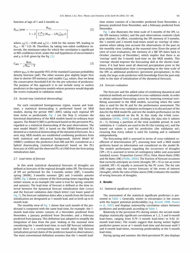
In this work statisticaledynamical forecasts of droughts aredefined as forecasts of the regional drought index SPI. The forecastsof SPI are performed for the 3-months winter (DJF), 3-monthsspring (MAM), 3-months summer (JJA) and 3-months autumn(SON). Fig. 5 shows a scheme of the forecasting times regarding thewinter season, as an example (the same is true for spring, summerand autumn). The lead-time of forecast is defined as the time in-terval between the dynamical forecast initialization date (cross)and the forecast validation date (black letter) (see lower panel ofFig. 5). The forecast validation dates after a month from the forecastinitialization are designated as 1-month lead, and so forth up to 6-month lead.

The monthly view of Fig. 5 shows that each month of the pre-dictand is computed with the same lead-time, for example: the 1-month lead-time winter consists of a December predicted fromNovember, a January predicted from December, and a Februarypredicted from January. This definition was adopted to simplify theintegration of data from the past: looking at the seasonal viewconsidering the 1-month lead-time, to each DJF forecast validationperiod there is a corresponding one month delay NDJ forecastinitialization period (dates of the predictors based on observations).The most conventional definition assumes that the 1-month lead-

time winter consists of a December predicted from November, aJanuary predicted from November, and a February predicted fromNovember.

Fig. 5 also illustrates the time-scale of 3-months of the SPI, i.e.the SPI memory (white), and the past observations contents (darkgray shadow). In effect, considering the SPI memory of 3-months,the 1-month and 2-month lead-times entail an ‘overlap’ of infor-mation when taking into account the observations of the past onthe monthly view. Looking at the seasonal view (from the point ofview of score evaluation), the memory of a DJF SPI dates back toOctober (memory of December), which implies that there is an‘overlap’ until the 5-month lead-time on the MLR models. This‘overlap’ should improve the forecasting skill at the shorter lead-times, if it had been used all observed precipitation prior to theforecasting initialization time (corresponding to the time-scale ofthe SPI) as additional predictors (persistent precipitation). In thisstudy, the large-scale predictors with knowledge from the past onlyrefer to the date of initialization of the dynamical forecasts.

2.8. Forecast evaluation

The forecasts and the added value of combining dynamical andstatistical methods are evaluated in cross-validation mode, in orderto obtain unbiased forecasting scores by removing eventual over-fitting associated to the MLR models, occurring when the samedata is used for the fit and for the performance assessment. Thebasic idea of the cross-validation techniques is to discard part of thedata for the MLR model fit, and test the models performance on thedata not considered on the fit. In this study the k-fold cross-validation (Wilks, 2006) is used, dividing the data into k subsets(k ¼ 3), forming a partition of the total available period. In eachvalidation, k�1 subsets are used to the fit (the training set), and theleaved out subset is used for prediction (the validation set),ensuring that every subset is used for training and is validatedindependently.

The forecasting skill is assessed in terms of cross-validated co-efficient of determination (R2), assessing how well a MLR modelperforms based on information not considered on the model fit.The models performance regarding the occurrence of droughts(SPI < 0) is assessed in terms of contingency tables and associatedstandard scores: Proportion Correct (PCo), False Alarm Ratio (FAR)and Hit Ratio (HR) (Wilks, 2006). The fraction of forecast occasionsthat correctly anticipate an event (drought, SPI < 0) or not an event(rainfall, SPI > 0) equally is assessed by the PC score. The hit rate(HR) regards only the correct forecasts of the event of interest(drought), while the ratio of false alarm (FAR) evaluates the numberof wrong forecasts of droughts.

3. Results

3.1. Statistical significant predictors

The assessment of the statistical significant predictors is pre-sented in Table 1. Generally, winter in extratropics is the seasonwith the largest potential predictability (e.g. Rowell, 1998; Davieset al., 1997) and displays noteworthy correlation values betweenpredictors and predictands according to Table 1.

Relatively to the persistent PCs during winter, the second modedisplays statistically significant correlations at 1, 2, 5 and 6-monthlead-times, ranging from 0.79 (1-month lead-time) to 0.42 (6-month lead-time). The results suggest that during winter higherpredictive power occur at 1-month lead-time and decrease until 3and 4-month lead-times, recovering predictability at the 5-monthlead-time.

During spring and summer, the third persistent PC also displays

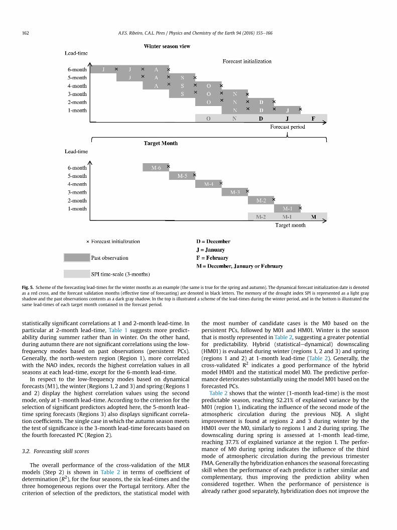
Fig. 5. Scheme of the forecasting lead-times for the winter months as an example (the same is true for the spring and autumn). The dynamical forecast initialization date is denotedas a red cross, and the forecast validation months (effective time of forecasting) are denoted in black letters. The memory of the drought index SPI is represented as a light grayshadow and the past observations contents as a dark gray shadow. In the top is illustrated a scheme of the lead-times during the winter period, and in the bottom is illustrated thesame lead-times of each target month contained in the forecast period.

A.F.S. Ribeiro, C.A.L. Pires / Physics and Chemistry of the Earth 94 (2016) 155e166162

statistically significant correlations at 1 and 2-month lead-time. Inparticular at 2-month lead-time, Table 1 suggests more predict-ability during summer rather than in winter. On the other hand,during autumn there are not significant correlations using the low-frequency modes based on past observations (persistent PCs).Generally, the north-western region (Region 1), more correlatedwith the NAO index, records the highest correlation values in allseasons at each lead-time, except for the 6-month lead-time.

In respect to the low-frequency modes based on dynamicalforecasts (M1), thewinter (Regions 1, 2 and 3) and spring (Regions 1and 2) display the highest correlation values using the secondmode, only at 1-month lead-time. According to the criterion for theselection of significant predictors adopted here, the 5-month lead-time spring forecasts (Regions 3) also displays significant correla-tion coefficients. The single case inwhich the autumn seasonmeetsthe test of significance is the 3-month lead-time forecasts based onthe fourth forecasted PC (Region 2).

3.2. Forecasting skill scores

The overall performance of the cross-validation of the MLRmodels (Step 2) is shown in Table 2 in terms of coefficient ofdetermination (R2), for the four seasons, the six lead-times and thethree homogeneous regions over the Portugal territory. After thecriterion of selection of the predictors, the statistical model with

the most number of candidate cases is the M0 based on thepersistent PCs, followed by M01 and HM01. Winter is the seasonthat is mostly represented in Table 2, suggesting a greater potentialfor predictability. Hybrid (statisticaledynamical) downscaling(HM01) is evaluated during winter (regions 1, 2 and 3) and spring(regions 1 and 2) at 1-month lead-time (Table 2). Generally, thecross-validated R2 indicates a good performance of the hybridmodel HM01 and the statistical model M0. The predictive perfor-mance deteriorates substantially using themodel M01 based on theforecasted PCs.

Table 2 shows that the winter (1-month lead-time) is the mostpredictable season, reaching 52.21% of explained variance by theM01 (region 1), indicating the influence of the second mode of theatmospheric circulation during the previous NDJ. A slightimprovement is found at regions 2 and 3 during winter by theHM01 over the M0, similarly to regions 1 and 2 during spring. Thedownscaling during spring is assessed at 1-month lead-time,reaching 37.7% of explained variance at the region 1. The perfor-mance of M0 during spring indicates the influence of the thirdmode of atmospheric circulation during the previous trimesterFMA. Generally the hybridization enhances the seasonal forecastingskill when the performance of each predictor is rather similar andcomplementary, thus improving the prediction ability whenconsidered together. When the performance of persistence isalready rather good separately, hybridization does not improve the

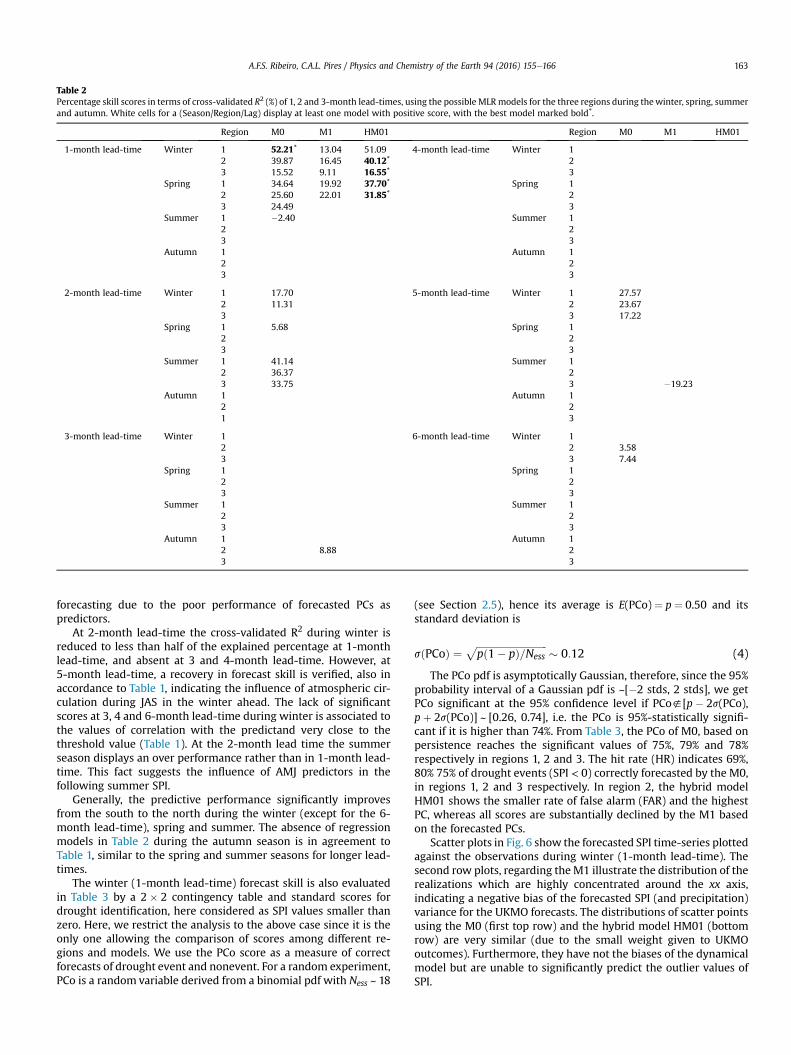
Table 2Percentage skill scores in terms of cross-validated R2 (%) of 1, 2 and 3-month lead-times, using the possible MLRmodels for the three regions during thewinter, spring, summerand autumn. White cells for a (Season/Region/Lag) display at least one model with positive score, with the best model marked bold*.

Region M0 M1 HM01 Region M0 M1 HM01

1-month lead-time Winter 1 52.21* 13.04 51.09 4-month lead-time Winter 12 39.87 16.45 40.12* 23 15.52 9.11 16.55* 3

Spring 1 34.64 19.92 37.70* Spring 12 25.60 22.01 31.85* 23 24.49 3

Summer 1 �2.40 Summer 12 23 3

Autumn 1 Autumn 12 23 3

2-month lead-time Winter 1 17.70 5-month lead-time Winter 1 27.572 11.31 2 23.673 3 17.22

Spring 1 5.68 Spring 12 23 3

Summer 1 41.14 Summer 12 36.37 23 33.75 3 �19.23

Autumn 1 Autumn 12 21 3

3-month lead-time Winter 1 6-month lead-time Winter 12 2 3.583 3 7.44

Spring 1 Spring 12 23 3

Summer 1 Summer 12 23 3

Autumn 1 Autumn 12 8.88 23 3

A.F.S. Ribeiro, C.A.L. Pires / Physics and Chemistry of the Earth 94 (2016) 155e166 163

forecasting due to the poor performance of forecasted PCs aspredictors.

At 2-month lead-time the cross-validated R2 during winter isreduced to less than half of the explained percentage at 1-monthlead-time, and absent at 3 and 4-month lead-time. However, at5-month lead-time, a recovery in forecast skill is verified, also inaccordance to Table 1, indicating the influence of atmospheric cir-culation during JAS in the winter ahead. The lack of significantscores at 3, 4 and 6-month lead-time during winter is associated tothe values of correlation with the predictand very close to thethreshold value (Table 1). At the 2-month lead time the summerseason displays an over performance rather than in 1-month lead-time. This fact suggests the influence of AMJ predictors in thefollowing summer SPI.

Generally, the predictive performance significantly improvesfrom the south to the north during the winter (except for the 6-month lead-time), spring and summer. The absence of regressionmodels in Table 2 during the autumn season is in agreement toTable 1, similar to the spring and summer seasons for longer lead-times.

The winter (1-month lead-time) forecast skill is also evaluatedin Table 3 by a 2 � 2 contingency table and standard scores fordrought identification, here considered as SPI values smaller thanzero. Here, we restrict the analysis to the above case since it is theonly one allowing the comparison of scores among different re-gions and models. We use the PCo score as a measure of correctforecasts of drought event and nonevent. For a random experiment,PCo is a random variable derived from a binomial pdf with Ness ~ 18

(see Section 2.5), hence its average is E(PCo) ¼ p ¼ 0.50 and itsstandard deviation is

sðPCoÞ ¼ffiffiffiffiffiffiffiffiffiffiffiffiffiffiffiffiffiffiffiffiffiffiffiffiffiffiffiffiffipð1� pÞ=Ness

p� 0:12 (4)

The PCo pdf is asymptotically Gaussian, therefore, since the 95%probability interval of a Gaussian pdf is ~[�2 stds, 2 stds], we getPCo significant at the 95% confidence level if PCo;[p � 2s(PCo),p þ 2s(PCo)] ~ [0.26, 0.74], i.e. the PCo is 95%-statistically signifi-cant if it is higher than 74%. From Table 3, the PCo of M0, based onpersistence reaches the significant values of 75%, 79% and 78%respectively in regions 1, 2 and 3. The hit rate (HR) indicates 69%,80% 75% of drought events (SPI < 0) correctly forecasted by the M0,in regions 1, 2 and 3 respectively. In region 2, the hybrid modelHM01 shows the smaller rate of false alarm (FAR) and the highestPC, whereas all scores are substantially declined by the M1 basedon the forecasted PCs.

Scatter plots in Fig. 6 show the forecasted SPI time-series plottedagainst the observations during winter (1-month lead-time). Thesecond row plots, regarding theM1 illustrate the distribution of therealizations which are highly concentrated around the xx axis,indicating a negative bias of the forecasted SPI (and precipitation)variance for the UKMO forecasts. The distributions of scatter pointsusing the M0 (first top row) and the hybrid model HM01 (bottomrow) are very similar (due to the small weight given to UKMOoutcomes). Furthermore, they have not the biases of the dynamicalmodel but are unable to significantly predict the outlier values ofSPI.

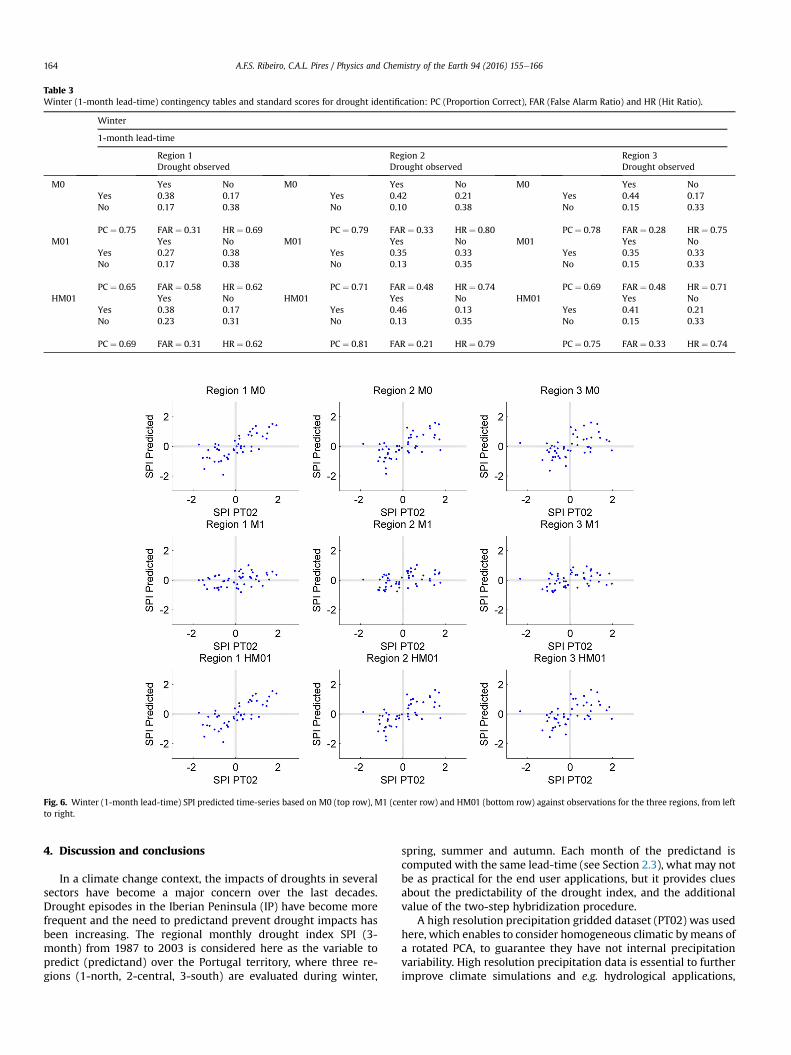
Table 3Winter (1-month lead-time) contingency tables and standard scores for drought identification: PC (Proportion Correct), FAR (False Alarm Ratio) and HR (Hit Ratio).

Winter

1-month lead-time

Region 1 Region 2 Region 3Drought observed Drought observed Drought observed

M0 Yes No M0 Yes No M0 Yes NoYes 0.38 0.17 Yes 0.42 0.21 Yes 0.44 0.17No 0.17 0.38 No 0.10 0.38 No 0.15 0.33

PC ¼ 0.75 FAR ¼ 0.31 HR ¼ 0.69 PC ¼ 0.79 FAR ¼ 0.33 HR ¼ 0.80 PC ¼ 0.78 FAR ¼ 0.28 HR ¼ 0.75M01 Yes No M01 Yes No M01 Yes No

Yes 0.27 0.38 Yes 0.35 0.33 Yes 0.35 0.33No 0.17 0.38 No 0.13 0.35 No 0.15 0.33

PC ¼ 0.65 FAR ¼ 0.58 HR ¼ 0.62 PC ¼ 0.71 FAR ¼ 0.48 HR ¼ 0.74 PC ¼ 0.69 FAR ¼ 0.48 HR ¼ 0.71HM01 Yes No HM01 Yes No HM01 Yes No

Yes 0.38 0.17 Yes 0.46 0.13 Yes 0.41 0.21No 0.23 0.31 No 0.13 0.35 No 0.15 0.33

PC ¼ 0.69 FAR ¼ 0.31 HR ¼ 0.62 PC ¼ 0.81 FAR ¼ 0.21 HR ¼ 0.79 PC ¼ 0.75 FAR ¼ 0.33 HR ¼ 0.74

Fig. 6. Winter (1-month lead-time) SPI predicted time-series based on M0 (top row), M1 (center row) and HM01 (bottom row) against observations for the three regions, from leftto right.

A.F.S. Ribeiro, C.A.L. Pires / Physics and Chemistry of the Earth 94 (2016) 155e166164

4. Discussion and conclusions

In a climate change context, the impacts of droughts in severalsectors have become a major concern over the last decades.Drought episodes in the Iberian Peninsula (IP) have become morefrequent and the need to predictand prevent drought impacts hasbeen increasing. The regional monthly drought index SPI (3-month) from 1987 to 2003 is considered here as the variable topredict (predictand) over the Portugal territory, where three re-gions (1-north, 2-central, 3-south) are evaluated during winter,

spring, summer and autumn. Each month of the predictand iscomputed with the same lead-time (see Section 2.3), what may notbe as practical for the end user applications, but it provides cluesabout the predictability of the drought index, and the additionalvalue of the two-step hybridization procedure.

A high resolution precipitation gridded dataset (PT02) was usedhere, which enables to consider homogeneous climatic bymeans ofa rotated PCA, to guarantee they have not internal precipitationvariability. High resolution precipitation data is essential to furtherimprove climate simulations and e.g. hydrological applications,

A.F.S. Ribeiro, C.A.L. Pires / Physics and Chemistry of the Earth 94 (2016) 155e166 165

given the strong dependency of precipitation on orography and avariety of precipitation regimes in the IP (Belo-Pereira et al., 2011).

An added effort to bring together dynamical seasonal forecastsand statistical methods has come up to address the shortcomingsassociated to forecasting skills. In order to improve seasonaldrought forecasts over Portugal, a two-step hybrid downscalingapproach based on statisticaledynamical techniques is presented.This work purposes a two-step hybrid scheme combining dynam-ical model forecasts and past observations as predictors on a sta-tistical downscaling approach. The performed statistical/hybriddownscaling is based on MLR models, which are widely used,standing out for their modest computing requirements and easyimplementation.

The pre-selection of the statistically significant predictors leadto 28 downscaling models with a positive validation score,considering all seasons, lead-times and regions altogether. At thesame time, in comparison with the downscaling performed overthe training period (without cross-validation, not shown), theexplained variance (R2) of the drought index is smaller, howevermore accurate, given the overcoming of the problems associated toover-fitting.

A source of predictability over Europe is the influence of thepersistent atmospheric circulation patterns. One of the goals of thisstudy is to take advantage of the skill of the dynamical models inforecasting the low-frequency variability, and enhance the fore-casting skill with the additional value of the most recent reanalysisfrom ECMWF (ERA-Interim) in representing large-scale features.The second (in winter) and third (in spring) persistent PCs of z500and the second forecasted PC (in both seasons) are the mostcorrelated low-frequency modes of variability at the shorter lead-time (1 month). It would be expected that the first mode of vari-ability exhibited the strongest connection to the drought indexbecause it is commonly linked to NAO, particularly during winter.However, the use of three months and not an average value of theseason for the PCA may be capturing the pattern that is moreassociated with precipitation in other modes.

Results suggest that winter is very predictable, particularly forthe shorter lead-time (1-month lead-time). The model M1 ratherdeteriorates the predictive ability and the hybrid model HM01exhibit skill scores very similar to that of theM0 (Table 2). However,a very slight improvement is found by the hybrid model HM01upon the statistical downscaling based on the past M0 (Table 2).The rate of hit a drought event displays the more accurate forecastsusing the M0 and the rate of false alarm is substantially discredit-able based on the M1 (Table 3). The results propose that theknowledge of the recent past displays the predominant effect,mainly for the shorter lead-time. These findings suggest that theuse of the dynamical model forecasts can lead to inaccuracies in thedrought index forecasting skill assessment, showing the addedvalue of the integration of past information from reanalysis on thedynamical forecasts.

The persistent PCs which exhibit more influence in winter (DJF)at 1, 2 and 5-month lead-times, are the second mode during NDJand OND (1 and 2-month lead-times respectively), and the firstmode during JAS (5-month lead-time) (see Fig. 5 and Table 2). Partof this influence between DJF and the 1 and 2-month lead-times isrelated to the here used intrinsic memory of 3-months of SPI pre-dictand, which reflects the influence of the previous atmosphericcirculation on agricultural droughts in Portugal. In addition, theresults suggests that previous summer and previous early autumnpredictors are potential predictors of winter SPI (here 5-monthlead-time).

Generally, the predictive performance significantly improvesfrom the region 3 (south) to the region 1 (north) (Table 2), sug-gesting a dependency in latitude. The region comprising the areas

with more cumulative precipitation in Portugal features the bestskill scores, reaching more than 50% of explained variance duringwinter (1-month lead-time) using M0 and HM01 (Table 2).

Taking together the results suggest that both purely statisticaldownscaling based on the persistent PCs (M0) and hybrid down-scaling (HM01) are adequate for estimating the regional SPI (3-months), although the predictive power of the large-scale fieldsbased on past observations (persistence) stands out. The results addsubstantial information on the use of seasonal predictions forregional drought predictability, in particular in Portugal, and maycontribute to the predictability of crops yields.

Conflicts of interest

The authors declare that there are no conflicts of interest.

Acknowledgments

This research was developed at IDL with the support of thePortuguese Foundation for Science and Technology (FCT) throughproject PTDC/GEOMET/3476/2012 e Predictability assessment andhybridization of seasonal drought forecasts in Western Europe(PHDROUGHT). The authors are thankful to the IPMA (InstitutoPortugues do Mar e da Atmosfera) for the precipitation data used inthis study (PT02 precipitation Dataset). The authors are alsosincerely thankful to Ricardo Trigo for his valuable suggestions andto two anonymous reviewers for their constructive comments.

References

Belo-Pereira, M., Dutra, E., Viterbo, P., 2011. Evaluation of global precipitation datasets over the Iberian Peninsula. J. Geophys. Res. 116, D20101. http://dx.doi.org/10.1029/2010JD015481.

Brankovic, C., Palmer, T.N., Ferranti, L., 1994. Predictability of seasonal atmosphericvariations. J. Clim. 7, 217e237.

Cleveland, R.B., Cleveland, W.S., McRae, J.E., Terpenning, I., 1990. STL: a seasonal-trend decomposition procedure based on loess. J. Official Stat. 6, 3e73.

Coelho, C.A.S., Costa, S.M.S., 2010. Challenges for integrating seasonal climateforecasts in user applications. Curr. Opin. Environ. Sustain. 2, 317e325.

Coelho, C.A.S., Stephenson, D.B., Balmaseda, M., Doblas-Reys, F.J., vanOldenborgh, G.J., 2006. Toward an integrated seasonal forecasting system forSouth America, America. J. Climate 19, 3704e3721.

Davies, J.R., Rowell, D.P., Folland, C.K., 1997. North Atlantic and European seasonalpredictability using an ensemble of multidecadal atmospheric GCM Simula-tions. Int. J. Climatol. 17, 1263e1284.

deCastro, M., Lorenzo, N., Taboada, J.J., Sarmiento, M., Alvarez, I., Gomez-Gesteira, M., 2006. Influence of teleconnection patterns on precipitation vari-ability and on river flow regimes in the Mi~no River basin (NW Iberian Penin-sula). Climate Res. 32, 63e73.

D�equ�e, M., Stroe, R., 1994. Formulation of Gaussian probability forecasts based onmodel extended-range integrations. Tellus 46A, 52e65.

Doblas-Reyes, F.J., Weisheimer, A., D�equ�e, M., Keenlyside, N., Mcvean, M.,Murphy, J.M., Rogel, P., Smith, D., Palmer, T.N., 2009. Addressing model uncer-tainty in seasonal and annual dynamical ensemble forecasts. Q. J. R. Meteorol.Soc. 135, 1538e1559.

Esteban-Parra, M.J., Rodrigo, F.C., Castro-Díez, Y., 1998. Spatial and temporal pat-terns of precipitation in Spain for the period 1880e1992. Int. J. Climatol. 18,1557e1574.

Folland, C.K., Scaife, A.A., Lindesay, J., Stephenson, D.B., 2012. How potentiallypredictable is the northern European winter climate a season ahead? Int. J.Climatol. 32, 801e808.

García-Herrera, R., Paredes, D., Trigo, R.M., Trigo, I.F., Hern�andez, E., Barriopedro, D.,Mendes, M.A., 2007. The outstanding 2004e05 drought in the Iberian Penin-sula: associated atmospheric circulation. J. Hydrometeorol. 8, 469e482.

Giorgi, F., Lionello, P., 2008. Climate change projections for the mediterranean re-gion, global planet. Change 63, 90e104.

Gouveia, C., Trigo, R.M., DaCamara, C.C., 2009. Drought and vegetation stressmonitoring in Portugal using satellite data. Nat. Hazards Earth Syst. Sci. 9,185e195. http://dx.doi.org/10.5194/nhess-9-185-2009.

Gouveia, C.M., Bastos, A., Trigo, R.M., DaCamara, C.C., 2012. Drought impacts onvegetation in the pre- and post-fire events over Iberian Peninsula. Nat. HazardsEarth Syst. Sci. 12, 3123e3137.

Hannachi, A., Jolliffe, I.T., Stephenson, D.B., 2007. Empirical orthogonal functionsand related techniques in atmospheric science: a review. Int. J. Climatol. 27,1119e1152. http://dx.doi.org/10.1002/joc.1499.

A.F.S. Ribeiro, C.A.L. Pires / Physics and Chemistry of the Earth 94 (2016) 155e166166

Hurrel, J.W., 1995. Decadal trends in the North Atlantic Oscillation: regional tem-peratures and precipitation. Science 269, 676e679.

Kim, H., Webster, P.J., 2010. Extended-range seasonal hurricane forecasts for theNorth Atlantic with a hybrid dynamical-statistical model. Geophys. Res. Lett. 37,L21705. http://dx.doi.org/10.1029/2010GL044792.

Kim, H., Webster, P.J., Curry, J.A., 2012. Seasonal prediction skill of ECMWF System 4and NCEP CFSv2 retrospective forecast for the Northern Hemisphere Winter.Clim. Dyn. 39, 2957e2973.

Martins, D.S., Raziei, T., Paulo, A.A., Pereira, L.S., 2012. Spatial and temporal vari-ability of precipitation and drought in Portugal. Nat. Hazards Earth Syst. Sci. 12,1493e1501.

McKee, T.B., Doeskin, N.J., Kleist, J., 1993. The relationship of drought frequency andduration to time scales. In: Eighth Conf. on Applied Climatology, AmericanMeteorological Society, pp. 179e184.

Morid, S., Smakhtin, V., Bagherzadeh, K., 2007. Drought forecasting using artificialneural networks and time series of drought indices. Int. J. Climatol. 27,2103e2111.

Palmer, W.C., 1965. Meteorological Drought. US Weather Bureau, 45, p. 58.Peng, Z., Wang, Q.J., Bennet, J.C., Schepen, A., Pappenberger, F., Pokhrel P., Wang, Z.,

2014. Statistical calibration and bridging of ECMWF System4 for forecastingseasonal precipitation over China. J. Geophys. Res. Atmos. 119. http://dx.doi.org/10.1002/2013JD021162.

Pires, C., 1996. Pr�evision Atmosph�erique �a Long-Terme: Un Probl�eme d’HybridationStatistico-Dynamique. Universit�e Pierre et Marie Curie, Paris, Th�ese de Doctorat.

Pires, C.A., Perdig~ao, R.A.P., 2007. Non-Gaussianity and asymmetry of the wintermonthly precipitation estimation from the NAO. Mon. Wea. Rev. 135, 430e448.

Pozo-V�azquez, D., Esteban-Parra, M.J., Rodrigo, F.S., Castro-Díez, Y., 2001. The as-sociation between ENSO and winter atmospheric circulation and temperaturein the north Atlantic region. J. Clim. 14, 3408e3420.

Raziei, T., Martins, D.S., Bordi, I., Santos, J.F., Portela, M.M., Pereira, L.S., Sutera, A.,2014. SPI modes of drought spatial and temporal variability in portugal:comparing observations, PT02, and GPCC gridded datasets. Water Resour.Manage. 25634. http://dx.doi.org/10.1007/s11269-014-0690-3.

Rodriguez-Puebla, C., Encinas, A.H., Nieto, S., Garmendia, J., 1998. Spatial andtemporal patterns of annual precipitation variability over the Iberian Peninsula.Int. J. Climatol. 18, 299e316.

Rodríguez-Puebla, C., Encinas, A.H., S�aenz, J., 2001. Winter precipitation over theIberian Peninsula and its relationship to circulation indices. Hydrol. Earth Syst.Sci. 5 (2), 233e244.

Rowell, D.P., 1998. Assessing potential seasonal predictability with an ensemble ofmultidecadal GCM simulations. J. Clim. 11, 109e119.

Sarda, J., Plaut, G., Pires, C., Vautard, R., 1996. Statistical and dynamical long-rangeatmospheric forecasts. Exp. Comp. Hybridization Tellus 48A, 518e537.

Sousa, P.M., Trigo, R.M., Aizpurua, P., Nieto, R., Gimeno, L., Garcia-Herrera, R., 2011.Trends and extremes of drought indices throughout the 20th century in theMediterranean. Nat. Hazards Earth Syst. Sci. 11, 33e51.

Trigo, R.M., Pozo-V�azquez, D., Osborn, T.J., Castro-Díez, Y., G�amiz-Fortis, S., Esteban-Parra, M.J., 2004. North Atlantic Oscillation influence on precipitation, river flowand water re-sources in the Iberian Peninsula. Int. J. Climatol. 24, 925e944.

Trigo, R.M.R., Garcia-Herrera, Díaz, J., Trigo, I.F., Valente, M.A., 2005. How

exceptional was the early August 2003 heatwave in France. Geophys. Res. Lett.32, L10701. http://dx.doi.org/10.1029/2005GL022410.

Trigo, R.M., A~nel, J.A., Barriopedro, D., García-Herrera, R., Gimeno, L., Nieto, R.,Castillo, R., Allen, M.R., Massey, N., 2013. The record winter drought of 2011e12in the Iberian Peninsula. Bull. Am. Meteorol. Soc. 94 (9), S41eS45.

Van den Dool, H.M., 1994. Long-range weather forecasts through numerical andempirical methods. Dyn. Atmos. Oceans 20, 247e270.

Van den Dool, H.M., Saha, S., 1990. Frequency dependence in forecast skill. Mon.Weather Rev. 118, 128e137.

Vautard, R., Pires, C., Plaut, G., 1996. Long-range atmospheric predictability usingspace-time principal components. Mon. Weather Rev. 124, 288e307.

Vicente-Serrano, S.M., 2005. El Ni~no and LA Ni~na influence on droughts at differenttimescales in the Iberian Peninsula. Water Resour. Res. 41, W12415.

Vicente-Serrano, S.M., 2006. Differences in spatial patterns of drought on differenttime scales: an analysis of the Iberian Peninsula. Water Resour. Manage 20,37e60. http://dx.doi.org/10.1007/s11269-006-2974-8.

Vicente-Serrano, S.M., 2007. Evaluating the impact of drought using remote sensingin a mediterranean, semi-arid region. Nat. Hazards 40, 173e208. http://dx.doi.org/10.1007/s11069-006-0009-7.

Vicente-Serrano, S.M., L�opez-Moreno, J.I., 2006. The influence of atmospheric cir-culation at different spatial scales on winter drought variability through a semi-arid climatic gradient in Northeast Spain. Int. J. Climatol. 26 (11), 1427e1453.

Vicente-Serrano, S.M., Beguería, S., L�opez-Moreno, J.I., 2010. A multiscalar droughtindex sensitive to global warming: the standardized precipitation evapotrans-piration index. J. Climate 23, 1696e1718.

Vicente-Serrano, S.M., Gouveia, C., Camarero, J.J., Begería, S., Trigo, R., L�opez-Mor-eno, J.I., Azorín-Molina, C., Pasho, E., Lorenzo-Lacruz, J., Revuleto, J., Mor�an-Tejedam E., Sanchez-Lorenzo, A., 2013. Response of vegetation to drought time-scales across global land biomes, PNAS 2013 110 (1) 52e57, http://dx.doi.org/10.1073/pnas.1207068110.

Vicente-Serrano, S.M., Lopez-Moreno, J.I., Berguería, S., Lorenzo-Lacruz, J., Sanchez-Lorenzo, A., García-Ruiz, J.M., Azorin-Molina, C., Mor�an-Tejeda, E., Revuelto, J.,Trigo, R., Coelho, F., Espejo, F., 2014. Evidence of increasing drought severitycaused by temperature rise in southern Europe. Environ. Res. Lett. 9, 044001.

Vitart, F., 2014. Evolution of ECMWF sub-seasonal forecast skill scores. Q.J.R.Meteorol. Soc. http://dx.doi.org/10.1002/qj.2256.

Vitart, F., Huddleston, M.R., D�equ�e, M., Peake, D., Palmer, T.N., Stockdale, T.N.,Davey, M.K., Weisheimer, A., 2007. Dynamically-based seasonal forecasts ofAtlantic tropical storm activity issued in June by EUROSIP. Geophys. Res. Lett. 34http://dx.doi.org/10.1029/2007GL030740.

von Storch, H., Zwiers, F.W., 1999. Statistical Analysis in Climate Research. Cam-bridge University Press, Cambridge, 484.

Wilks, D.S., 2006. Statistical Methods in the Atmospheric Sciences, second ed. Ac-ademic Press, Amsterdam.

Zhu, H., Wheeler, M.C., Sobel, A.H., Hudson, D., 2014. Seamless precipitation pre-diction skill in the tropics and extratropics from a global model. Mon. WeatherRev. 142, 1556e1569.

Zieba, A., 2010. Effective number of observations and unbiased estimators of vari-ance for autocorrelated data e an overview. Metrol. Meas. Syst. 17 (1), 3e16.http://dx.doi.org/10.2478/v10178-010-0001-0.