seasonal prediction of the indian summer monsoon: … seminar on seasonal prediction, 3-7 september...

ECMWF Seminar on Seasonal Prediction, 3-7 September 2012 | 105

Seasonal prediction of the Indian summer monsoon: science and applications to Indian agriculture

Sulochana Gadgil Centre for Atmospheric and Oceanic Sciences, Indian Institute of Science, Bangalore 560012, India [email protected]

Abstract

With analysis of the impact of the monsoon on agriculture, it has been shown that reliable predictions of the extremes of the Indian summer monsoon rainfall (ISMR) and in particular of the non-occurrence of droughts can contribute to the enhancement of agricultural production with application of available technology. The strong association of the extremes of ISMR with ENSO and the equatorial Indian Ocean oscillation (EQUINOO) is discussed. Analysis of retrospective predictions by some models of ENSEMBLES and CFS1,2 of NCEP has shown that there is a great degree of coherence in monsoon predictions with almost all the models predicting the right sign of the ISMR anomaly for some extremes and almost all generating a loud false alarm for some seasons (1983 and 1997). The large errors in these seasons can be partly attributed to the poor skill in prediction of some facets of ENSO such as the transition from El Nino and the pattern of SST and rainfall anomalies associated with the mature phase. Poor skill in triggering the Indian Ocean Dipole event of 1997 also contributes to the poor skill in prediction of the 1997 monsoon. Thus, for improvement of skill in prediction of the Indian summer monsoon rainfall it is necessary to improve the prediction of both the critical modes (ENSO, EQUINOO).

1 Introduction “I seek the blessings of Lord Indra to bestow on us timely and bountiful monsoons” Pranab Mukherjee, budget speech in the LokSabha, February 2011.

This opening remark by the Indian finance minister in his presentation of the budget for 2011-12 in the parliament, drives home the point that the monsoon continues to have a substantial impact on the Indian agricultural production and economy, even after six decades of development during which the contribution of agriculture to GDP has come down from about 50% to less than 15%. Thus, understanding and prediction of the variability of the monsoon rainfall over the Indian region is extremely important. The finance minister’s concern was about the Indian summer monsoon rainfall (ISMR) during the forthcoming season. I shall also focus on the interannual variation of ISMR in this paper, with a special emphasis on the relationship of ISMR to events over the Pacific and Indian Oceans.

S. Gadgil: Seasonal prediction of the Indian summer monsoon

106 | ECMWF Seminar on Seasonal Prediction, 3-7 September 2012

It has been known for a long time that the Indian monsoon has an enormous impact on the agriculture and economy, with India’s economy being described as a gamble on the monsoon rains in the colonial era. A quantitative assessment of the impact is now available [Gadgil and Gadgil, 2006]. In this paper, after a brief discussion of the nature of the interannual variation of the ISMR, I elucidate the nature of the impact of the monsoon on the food grain production (FGP) in the country and the Gross Domestic Product (GDP), suggest an explanation for the observed nonlinear relationship of the impact to ISMR and show that seasonal predictions for the occurrence and non-occurrence of droughts, i.e. large deficits of ISMR, would be most useful for enhancing agricultural production in the face of the variability of the monsoon.

I consider next, the present understanding of the interannual variation of the Indian summer monsoon. A major advance in this occurred in the 80's with the discovery (or rediscovery) of a strong link with El Nino and Southern Oscillation, ENSO [Sikka, 1980; Pant and Parthasarathy, 1981; Rasmusson and Carpenter, 1983]. Recent studies [Gadgil et al., 2003, 2004; Ihara et al., 2007] have revealed that one more mode, viz. the Equatorial Indian Ocean Oscillation (EQUINOO), plays an important role in the interannual variation of ISMR. Gadgil et al., (2004) have shown that all the extremes of ISMR can be understood in terms of the favourable/unfavourable phases of these two modes. EQUINOO has been considered to be the atmospheric component of the Indian Ocean Dipole/zonal (IOD) mode (Saji. et al. 1999, Webster et al. 1999). However, the coupling between EQUINOO and the ocean component is weaker than that between the atmosphere and ocean components of ENSO. The study of Ihara et al.(2007) on the relationship of the variation of the monsoon with ENSO, EQUINOO and IOD, using data for a much longer period (from 1881 to 1998) than that used by Gadgil et al (2004), also suggests that the variation of ISMR is better described by use of indices of ENSO as well as EQUINOO (but not of ENSO and IOD).If it is possible to predict ENSO and EQUINOO for the forthcoming monsoon season, it will be possible to generate a reliable one-sided prediction i.e. non- occurrence of one of the extremes (i.e. either droughts or excess rainfall season).

The challenging problem of the simulation and prediction of ISMR with atmospheric and coupled models is discussed in the light of our understanding of the teleconnections of the interannual variation of the monsoon. Despite the strong link of the Indian /Asian monsoon with ENSO, AGCMs forced by the observed sea surface temperature (SST) under AMIP (Gates 1992), as well as a CLIVAR Monsoon Panel intercomparison project for 1997-98, showed poor skill in the simulation of its interannual variation (Sperber and Palmer 1996, Gadgil and Sajani 1998, Kang et al 2002, Wang et al.2004). Wang et al (2005) suggested that atmospheric models are inherently incapable of simulating the variability of the monsoon, even when they are forced by the observed SST, because of the special SST-rainfall relationship (as assessed by the correlation between the rainfall and local SST) over the warm oceanic regions such as South China Sea and tropical West Pacific. They concluded that there is a ‘Fundamental challenge in simulation and prediction of summer monsoon rainfall’ which calls for a reshaping of current strategies for monsoon seasonal prediction. If their hypothesis is true, coupled models as a class would have a higher skill than



AGCMs, in simulating the SST-rainfall relationship and hence the interannual variation of the monsoon.

It is, therefore important to elucidate the nature of the observed relationship between rainfall and local SST of tropical oceans and assess the skill of AGCMs and CGCMs in simulating it. The observed relationship of organized deep convection/high rainfall over tropical oceans to the local SST, is highly nonlinear, with a high propensity for deep convection/high rainfall for SST above a threshold of about 27.50C and a large spread in the convection/precipitation values for each SST for SSTs above the threshold (Gadgil et al 1984, Graham and Barnett 1987, Waliser and Graham 1993, Zhang 1993, Bony et al 1997, Rajendran et al 2012). For such a nonlinear relationship, correlation is not an appropriate measure (Graham and Barnett 1987). It has been shown that the correlation coefficient depends upon the range of SST and for SSTs above the threshold, the correlation between convection/rainfall and local SST becomes insignificant (Gadgil et al. 1984). In a recent study by Rajendran et al. (2012), the runs of the atmospheric and the coupled versions of nine global climate models used in the Fourth Assessment Report of the Intergovernmental Panel on Climate Change (IPCC AR4) were analysed. They have shown that the SST–rainfall relationship simulated by the AGCMs and CGCMs in IPCC AR4 is nonlinear, as observed, and realistic over the tropical West Pacific and the Indian Ocean as well as the Nino3.4 region. Furthermore, the SST–rainfall pattern simulated by the coupled versions of these models is found to be rather similar to that from the corresponding atmospheric one, except for a shift of the entire pattern to colder/warmer SSTs when there is a cold/warm bias in the coupled version. Thus it appears that poor skill of simulation and interannual variation of the monsoon by AGCMs cannot be attributed to their skill in simulating the SST-rainfall relationship over warm parts of the tropical Indian and Pacific Oceans and improvement of the atmospheric component of the models can contribute towards better simulation and prediction of the variability of the monsoon.

Finally, I discuss the skill of the state-of art coupled models in predicting ISMR, and in particular, the extremes. Recent studies have shown that there has been considerable improvement in the skill of retrospective predictions of ISMR with coupled models. While the correlation of the multi-model ensemble (MME) prediction with the observed ISMR for the models in DEMETER (Palmer et al.2004) was 0.22 (Preethi et al 2010) the correlation for the MME from six models of ENSEMBLES (http://www.ecmwf.int/research/EU_projects/ENSEMBLES/) is 0.45 (Rajeevan et al. 2012). However, despite considerable improvement over the last decade, none of the models at the global centres were able to predict the droughts of 2002, 2004 and 2009. Hence further improvement is essential.

A surprising result from the analysis of the predictions of the extremes by the six models of ENSEMBLES and the two versions CFS1 and CFS2 of the NCEP model is the coherence in the prediction of most of the extremes ISMR, despite the differences between the models. Thus the extremes for which almost all the models predict the correct sign of the ISMR anomalies include the seasons with strong ENSO signal such as 1987, 88 as well as those with a strong positive phase of EQUINOO associated with the IOD events such as 1961 and 1994. This coherence is seen the bad predictions as well. Almost all the models predict deficit ISMR for the excess monsoon season of 1983, and



large deficit for the monsoon season of 1997 with a positive ISMR anomaly. As expected, inadequate skill in prediction of the SST of the equatorial Indian Ocean and convection over that ocean contributes to the poor skill in prediction of for these seasons. However, it turns out that the large errors in the prediction of ISMR can be attributed also to the error in prediction of the timing of the transition from El Nino (e.g. 1983) and the strength and spatial patterns of anomalies characterizing the mature phase of El Nino (e.g. 1997). Thus improvement in prediction of some facets of ENSO as well as of triggering of positive IOD events is required for improvement of the skill of the models in monsoon prediction.

2 Interannual variation of the Indian summer monsoon rainfall Most of the rainfall over the Indian region as a whole occurs during the summer monsoon season of June-September. The large-scale summer monsoon rainfall is associated with a continental tropical convergence zone in the monsoon zone north of about 180N over the subcontinent. The value of ISMR, for any year, is a weighted average of the June-September rainfall at 306 well-distributed rainguage stations across India [Parthasarathy et al., 1992, 1995 and the web site of Indian Institute of Tropical Meteorology (http://www.tropmet.res.in/)]. In fact, ISMR is a very reliable facet of our atmosphere with the range of the interannual variation from 1870 onwards being 70% to 120% of the long term mean of about 85cms and the standard deviation, about 10% of the mean. The variation of ISMR from 1960 is shown in Figure 1. Seasons with the magnitude of the ISMR anomaly larger than one standard deviation (i.e. of normalized anomaly larger than 1) are extremes -droughts/ excess rainfall seasons for negative/positive anomaly. It is seen that droughts occurred very frequently during 1965-87 and after a lull during 1988-2001, the frequency has been high in the last decade with droughts in 2002, 2004 and 2009).

Figure 1: Variation of the anomaly of the Indian summer monsoon rainfall (ISMR), normalized by the standard deviation, during 1960-2011

3 Impact of the monsoon on agriculture and GDP The Indian food-grain production (FGP), and the GDP, have increased rapidly since independence (Figure 2a).It is seen that the FGP has grown exponentially at 2.7% during 1950-94, but slowed down since then to 1.2% , perhaps because of the fatigue of the green revolution (Gadgil and Gadgil 2006). The GDP grew at the ‘Hindu rate of



growth’ of 3.6% until 1980; grew more rapidly at 5.3% over the next two decades and even faster in the last decade (Figure 2b).Over and above these long term trends, there are year to year fluctuations which can be attributed to important events in the year and particularly the monsoon. The impact of the monsoon is taken as the difference between the observed value of FGP/GDP in a year and the value it would have if it grew according to the long term trend.

Figure 2: a Variation of the Indian foodgrain production (FGP) during 1950-2009. b Variation of the Indian Gross Domestic product (GDP) during 1950-2009 c Impact of the monsoon on the FGP versus ISMR anomaly d Impact of the monsoon on the GDP versus ISMR anomaly

The variation of the impact on FGP (IFGP), and on GDP (IGDP) with ISMR anomaly is shown in Figure 2c and d respectively. It is seen that the impact is highly nonlinear for FGP and GDP, with the negative impact of negative ISMR anomaly being much larger than the positive impact of an ISMR anomaly of the same magnitude. Furthermore, since 1980, while the negative impact of a deficit monsoon on FGP has remained as large as in during 1951-1980, the positive impact of a positive anomaly has decreased substantially (Table1). Over the last three decades, there have been major changes in the cropping patterns, due to various factors including larger impact of the market economy, availability of high yielding varieties etc. and the traditional complex cropping system is now replaced by mono-cropping over large tracts of land. This has led to a large number of pests and diseases becoming endemic. Furthermore, intensive farming has resulted in loss of fertility of the soil. In this situation, application of fertilizers and pesticides has become necessary for getting high yields. A comparison of



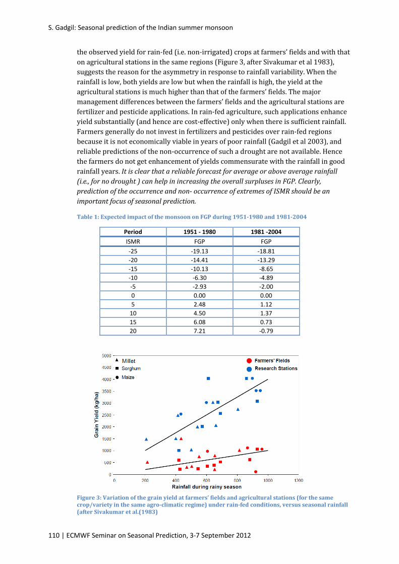
the observed yield for rain-fed (i.e. non-irrigated) crops at farmers’ fields and with that on agricultural stations in the same regions (Figure 3, after Sivakumar et al 1983), suggests the reason for the asymmetry in response to rainfall variability. When the rainfall is low, both yields are low but when the rainfall is high, the yield at the agricultural stations is much higher than that of the farmers’ fields. The major management differences between the farmers’ fields and the agricultural stations are fertilizer and pesticide applications. In rain-fed agriculture, such applications enhance yield substantially (and hence are cost-effective) only when there is sufficient rainfall. Farmers generally do not invest in fertilizers and pesticides over rain-fed regions because it is not economically viable in years of poor rainfall (Gadgil et al 2003), and reliable predictions of the non-occurrence of such a drought are not available. Hence the farmers do not get enhancement of yields commensurate with the rainfall in good rainfall years. It is clear that a reliable forecast for average or above average rainfall (i.e., for no drought ) can help in increasing the overall surpluses in FGP. Clearly, prediction of the occurrence and non- occurrence of extremes of ISMR should be an important focus of seasonal prediction.

Table 1: Expected impact of the monsoon on FGP during 1951-1980 and 1981-2004

Period 1951 - 1980 1981 -2004 ISMR FGP FGP -25 -19.13 -18.81 -20 -14.41 -13.29 -15 -10.13 -8.65 -10 -6.30 -4.89 -5 -2.93 -2.00 0 0.00 0.00 5 2.48 1.12

10 4.50 1.37 15 6.08 0.73 20 7.21 -0.79

Figure 3: Variation of the grain yield at farmers’ fields and agricultural stations (for the same crop/variety in the same agro-climatic regime) under rain-fed conditions, versus seasonal rainfall (after Sivakumar et al.(1983)



4 Interannual variation of the Indian summer monsoon: present understanding The correlation between ISMR and the OLR over the Indo-Pacific region for the summer monsoon (June-September) is shown in Figure 4. It is seen that there is a large negative correlation between the ISMR and convection/rainfall over the central Pacific. This is a manifestation of the link between the Indian summer monsoon and El Nino and Southern Oscillation [ENSO]. ISMR is also highly correlated with convection/rainfall over the western equatorial Indian Ocean and negatively correlated with the convection/rainfall over the eastern equatorial Indian Ocean. This is a manifestation of the link of ISMR with EQUINOO.

Figure 4: Correlation of ISMR with OLR at every grid point over 30E-70W and 40S-40N

The strong link between the ISMR and ENSO is manifested as an increased propensity of droughts during El Nino and of excess rainfall during La Nina (Sikka, 1980, Pant and Parthasarathy 1981, and Rasmusson and Carpenter 1983 etc.). To depict the relationship of the ISMR with ENSO, we use an ENSO index based on the SST anomaly of the Nino 3.4 region (120°-170°W, 5°S-5°N), since the magnitude of the correlation coefficient of ISMR with the convection over the central Pacific is higher than that with convection over the east Pacific (Figure 5). The ENSO index is defined as the negative of the Nino 3.4 SST anomaly (normalized by the standard deviation), so that positive values of the ENSO index imply a phase of ENSO favourable for the monsoon. El Nino events are associated with ENSO index less than -1.0 and La Nina with ENSO index greater than 1.0.

The relationship of ISMR with ENSO index is shown for the period 1958-2004 in Figure 5, in which the droughts and excess rainfall seasons of ISMR can also be distinguished. It is seen that ISMR is well correlated with the ENSO index with a correlation coefficient of 0.54 which is significant at 99%. When the ENSO index is favourable (>0.6), there are no droughts and when it is unfavourable (<-0.8) there are no excess monsoon seasons. However, for intermediate values of the ENSO index, there are several droughts and excess rainfall seasons. If we consider the interannual variation of the monsoon since 1980, consistent with the links of the monsoon with ENSO, the El Ninos of 1982 and 1987were associated with droughts and the La Nina of 1988with excess rainfall (Figure 4). It turned out that for 14 consecutive years



beginning with 1988, there were no droughts; furthermore, during the strongest El Nino event of the century in 1997, the ISMR was higher than the long-term mean (Figure 1) and Krishna Kumar et al.(1999) suggested that the relationship between the Indian monsoon and ENSO had weakened in the recent decades. Then came the drought of 2002, which occurred in association with a much weaker El Nino than that of 1997 and neither the statistical nor the dynamical models could predict it. The intriguing monsoon seasons of 1997 and 2002 triggered studies which suggested a link to events over the equatorial Indian Ocean (Gadgil et al. 2003, 2004).

Figure 5: Variation of ISMR with ENSO index (defined in the text)

The major difference between the OLR anomaly patterns for July 1997 (for which the all-India rainfall was close to the normal) and 2002 (for which the all-India rainfall was deficit by a massive 49%) is found to be over the equatorial Indian Ocean (Fig. 6a). Whereas in July 1997, the convection is enhanced over the western equatorial Indian Ocean and suppressed over the eastern equatorial Indian Ocean, the reverse is the case for July 2002.Suppression of convection over the eastern equatorial Indian Ocean (90° -110°E, 10°S-EQ, henceforth EEIO) tends to be associated with enhancement over the western equatorial Indian Ocean (50°-70°E, 10°S-10°N, henceforth WEIO) and vice versa. EQUINOO is the oscillation of a state with enhanced convection over WEIO and reduced convection over EEIO (positive phase) and another with anomalies of the opposite signs (negative phase). The positive phase of EQUINOO (e.g. Fig. 6b) is associated with easterly anomalies in the equatorial zonal wind; whereas the negative phase (i.e. with enhanced (suppressed) convection over the EEIO (WEIO)), is associated with westerly anomalies of the zonal wind at the equator. It is seen from Figure 6a that while the phase of ENSO in 1997 is the same as that in 2002, the phase of EQUINOO is positive in 1997 and negative in 2002. That a positive phase of EQUINOO with enhanced convection over WEIO is favourable for the monsoon is clearly seen from the pattern of the correlation of ISMR with OLR (Figure 4). It should be noted that the magnitude of the correlation of ISMR with the convection over WEIO is comparable to that with the convection over the central Pacific corresponding to the link with ENSO. We use an index of the EQUINOO based on the anomaly of the zonal component of the surface wind over the central equatorial region (CEIO, 60°E-90°E,



2.5°S-2.5°N), which is highly correlated (coefficient 0.79) with the difference between OLR of WEIO and EEIO. The zonal wind index (henceforth EQWIN) is taken as the negative of the anomaly so that positive values of EQWIN are favourable for the monsoon.

Figure 6a: OLR anomaly patterns for July 2002 (top) and July 1997 (bottom),

Figure 6b: Anomaly patterns of SST (left), OLR and surface wind (right) for June –September 1994 (top)and 1997(bottom)



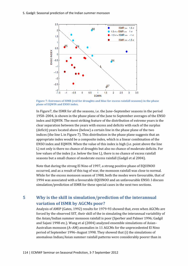
Figure 7: Extremes of ISMR (red for droughts and blue for excess rainfall seasons) in the phase plane of EQWIN and ENSO index.

In Figure7, the ISMR for all the seasons, i.e. the June–September seasons in the period 1958–2004, is shown in the phase plane of the June to September averages of the ENSO index and EQWIN. The most striking feature of the distribution of extreme years is the clear separation between the years with excess and deficits with each of the surplus (deficit) years located above (below) a certain line in the phase plane of the two indices (the line L in Figure 7). This distribution in the phase plane suggests that an appropriate index would be a composite index, which is a linear combination of the ENSO index and EQWIN. When the value of this index is high (i.e. point above the line L) not only is there no chance of droughts but also no chance of moderate deficits. For low values of the index (i.e. below the line L), there is no chance of excess rainfall seasons but a small chance of moderate excess rainfall (Gadgil et al 2004).

Note that during the strong El Nino of 1997, a strong positive phase of EQUINOO occurred, and as a result of this tug of war, the monsoon rainfall was close to normal. While for the excess monsoon season of 1988, both the modes were favourable, that of 1994 was associated with a favourable EQUINOO and an unfavourable ENSO. I discuss simulation/prediction of ISMR for these special cases in the next two sections.

5 Why is the skill in simulation/prediction of the interannual variation of ISMR by AGCMs poor? Analysis of AMIP (Gates, 1992) results for 1979-93 showed that, even when AGCMs are forced by the observed SST, their skill of the in simulating the interannual variability of the Asian/Indian summer monsoon rainfall is poor (Sperber and Palmer 1996; Gadgil and Sajani 1998 etc.). Wang et al (2004) analyzed ensemble simulations of Asian–Australian monsoon (A–AM) anomalies in 11 AGCMs for the unprecedented El Nino period of September 1996–August 1998. They showed that (i) the simulations of anomalous Indian/Asian summer rainfall patterns were considerably poorer than in



the El Nino region and (ii) the skill in the ensemble simulations with the SNU model for 1950-98 of the Indian monsoon is significantly higher than the skill for the period 1996–98. They concluded that ‘During 1997/98 El Nino, the models experienced unusual difficulty in reproducing correct Indian summer monsoon anomalies’.

Wang et al (2004) suggested that the cause of the models’ deficiencies is the failure to simulate correctly the relationship between the summer rainfall and the local SST over the Philippine Sea, the South China Sea, and the Bay of Bengal. This led to a paper on ‘Fundamental challenge in simulation and prediction of summer monsoon rainfall’ by Wang et al (2005) that has received a lot of attention. They examined the simulation skill of five state-of-the-art AGCMs, forced by identical observed SST and sea-ice, in seasonal precipitation for a 20-year period of 1979–1998. They pointed out that the correlations of the observed local SST and precipitation anomalies are negative over the West north Pacific and insignificant over the Bay of Bengal and that the SST-rainfall correlations in the MME simulation disagree with observations primarily in the Asian-Pacific monsoon regions. They attributed the unsuccessful simulations of the rainfall variability in the Asian-Pacific summer monsoon under AMIP-type experimental design to the neglect of air-sea interaction in the warm Indo-Pacific oceans, and suggest that the coupled atmosphere-ocean processes are extremely important in the heavily precipitating monsoon regions. On the other hand, Gadgil et al. (2005) attributed the poor skill of AGCMs to ) a poor skill in simulation of the monsoon-EQUINOO link.

In order to identify the strategy for improvement of the models, it is important to understand why the skill of the models is poor whether either of the hypotheses proposed are valid. We note that, if the Wang et al (2005) hypothesis is valid, the coupled models as a class would have higher skill than the AGCMs, in simulation SST-rainfall relationships over the warm Indo-Pacific oceans and hence also of the variability of the Indian/Asian monsoon. Thus it is important to assess the skill in simulation of the SST-rainfall relationship by AGCMs and CGCMs.

Consider first the nature of the observed relationship between convection/rainfall and local SST. The observed SST-rainfall relationship is highly nonlinear (Gadgil et al 1984, Graham and Barnett 1987, Waliser et al. 1993; Zhang 1993; Bony et al. 97; Lau and Sui 97etc.) It has been shown that, (i) there is a threshold of SST around 27.50C with a high propensity for organized convection /high rainfall over oceans with SST above the threshold. (ii) When the SST is above the threshold, the OLR/rainfall varies over a large range from almost no convection/rainfall to high rainfall/intense deep convection for each SST. The correlation coefficient between the local SST and the convection/rainfall depends on the range of SST (Gadgil et al . 1984). When SST varies over a large range across the threshold, the correlation is significantly positive (as for the Indian Ocean: 60°-100°E, 15°S-20°N ). However, for oceanic regions with SST maintained above the threshold (such as the Bay of Bengal, tropical West Pacific etc.) the correlation is insignificant (Gadgil et al 1984). Clearly, for such a nonlinear relationship, correlation is not an appropriate measure (Graham and Barnett 1987). However, in the Wang et al (2004,5) studies, simulation of the SST-rainfall relationship was assessed by a comparison of the observed and simulated correlation between the rainfall and local SST.



An important question that arises is: ‘How good are the simulations of tropical SST–rainfall relationship by atmospheric and coupled models?’ Rajendran et al. (2012) addressed this question, by analysis of the runs of atmospheric and coupled versions of nine IPCC AR4 climate models, for the present day climate. The observed relationship

Figure 8a For the Indian Ocean (IO: 60-100°E;15°S-20°N), Left:Observations of the relationship between rainfall and SST for June, July, August during 1979-2009: Scatter plot with the number of points for each 0.25_C SST and 0.5mm rainfall bin is shown above and the variation with SST of the 90% percentile of rainfall (blue curve), mean rainfall (black curve), and the standard deviation of rainfall (red curve) shown below. ; Right: Scatter plots for simulation by AGCM and CGCM (above) and variation with SST of the 90% percentile and the mean rainfall (below) for the GFDL, CNRM and IPSL models.

Figure 8b For WPO (120-140°E;10-20°N) Left: Observations of the relationship between rainfall and SST for June, July, August during 1979-2009: Scatter plot with the number of points for each 0.25_C SST and 0.5mm rainfall bin is shown above and the percentage of occurrence of the number of grids for each SST interval (below) Right: Scatter plots for simulation by AGCM and CGCM for GFDL and CNRM models



between rainfall and SST over the Indian Ocean (IO: 60°-100°E, 15°S-20°N ) tropical West Pacific (WPO:120°-140°E, 10°-20°N) is shown in Fig. 8a and b respectively. The frequency distribution of the observed SST for WPO is also shown in Fig. 8b. It is seen that overWPO, which is always maintained above the threshold, there is an enormous spread of rainfall values for each value of SST implying that the rainfall is not related to the local SST. Despite this, if the correlation coefficient is calculated, it turns out to be negative but it is not significant even at 90%.The simulated patterns by two AGCMs and the corresponding CGCMs over the region are also shown in Fig. 8b. Since the SST of WPO is always above the threshold, as observed, there is a large variation in the rainfall for each value of SST. The patterns simulated by the AGCMs are rather similar to those simulated by the corresponding CGCMs, except for a shift towards colder SSTs when there is a cold bias in the coupled version (such as CNRM ). Rajendran et al. (2012) have shown that the simulation of the SST-rainfall relationship by AGCMs as well as CGCMs over different regions such as the Indian Ocean, Nino 3.4 and WPO is realistic. This implies that the poor skill of AGCMs, forced by observed SSTs, in simulating the interannual variation of the monsoon, cannot be attributed to the skill in simulation of the special SST-rainfall relationship over warm oceans such as the tropical West Pacific.

Gadgil et al (2005)’s analysis of AMIP runs for 1979-94 showed that most of the AGCMs simulate the correct sign of the ISMR anomaly for the extremes of the monsoon associated with ENSO (e.g. excess monsoon of 1988 associated with La Nina in Fig. 9) but for extremes for which EQUINOO plays an important role (such as 1994 in which excess rainfall occurred despite a weak El Nino) most of the models cannot even simulate the sign of the ISMR anomaly (Fig. 9).Occurrence of large errors only for a few years suggests that the low skill in simulation of the interannual variation of the monsoon arises from a poor simulation of an important facet/phenomenon and/or of the teleconnections rather than the omission of an important process such as coupling. Note that 1994 and 1997 seasons are characterized by a positive phase of EQUINOO, associated with strong positive IOD events (Fig. 6b). The anomalies over the equatorial Indian Ocean associated with the positive phase of EQUINOO are generally simulated by the AGCMs forced with the observed SST. Hence, Gadgil et al (2005) suggested that poor skill in simulation of the monsoon-EQUINOO link leads to the poor skill of AGCMs in simulation of interannual variation of ISMR.

The poor skill in simulation of the monsoon –EQUINOO link could arise from an inherent inability in this set of models to simulate this link or on their response to EQUINOO vis a vis ENSO. Thus interannual variation of the monsoon could be attributed to either excessive sensitivity to ENSO or a poor skill in simulating the link of the monsoon with EQUINOO. Under a national atmospheric model intercomparison project on Seasonal Prediction of the Indian Monsoon (SPIM) involving five AGCMs, which were used in the country for monthly /seasonal predictions, retrospective predictions were generated for the summer monsoon seasons of 1985-2004 (Gadgil and Srinivasan 2011). For each model, 5 member ensemble runs were made with initial conditions specified from observations at the end of April. Two experiments were run; one in which the models were forced by the observed SST and the second in



Figure 9: Top:For June-September 1988: Observed ISMR anomaly (black), anomaly simulated by different models in AMIP. Bottom: same as top but for 1994

which the SST was derived by assuming that the April anomalies persisted. It was found that when forced by the observed SST, the local response over the equatorial Indian Ocean with a positive phase of the EQUINOO was well simulated for the season of 1994. However, the link with EQUINOO was not and the simulated ISMR anomaly was negative (as for AMIP ) instead of the observed large positive anomaly. However, in the second experiment, with the SST anomalies persisting from April onwards (which implied that the ENSO was weaker), the two best models (PUM and SFM, which were versions of the UKMET office model and the NCEP model respectively) could simulate the link with EQUINOO and a positive ISMR anomaly. Thus for these models, the simulation of deficit rainfall in 1994 when forced by observed SST resulted from hypersensitivity to ENSO rather than the lack of ability to simulate the monsoon-



EQUINOO link. . If that is indeed the case, just as the improvement in the simulation of the monsoon-ENSO link by AGCMs was achieved under international programme ‘MONEG’ in the nineties (under which the cases of 1987 and 1988 were studied with a slew of models) and efforts thereafter, it should be possible to improve the simulation of the monsoon –EQUINOO link even for realistic SST forcing.

To summarize, the lessons from the analysis of the simulation of the interannual variation of ISMR by AGCMs are: (i) AGCMs, when forced by the observed SST, are generally able to simulate the monsoon-ENSO link. Also, for some IOD events such as 1994 they are able to simulate the local response of a positive EQUINOO but not the monsoon-EQUINOO link and (ii) Some of the AGCMs do simulate the positive impact of positive phase of EQUINOO on ISMR in 1994 when forced by weaker SST anomalies (i.e. weaker EL Nino than observed). Thus the monsoon-EQUINOO link is not simulated by such models because of their unrealistically large response to ENSO. We, therefore, expect that AGCMs forced by observed SST should be able to simulate a positive ISMR anomaly for the season of 1961 which was also characterized by a positive IOD event and a favourable phase of ENSO.

6 Retrospective predictions by recent versions of coupled models Recent studies (e.g. Rajeevan et al. 2012) have shown that there has been considerable improvement in the skill of retrospective predictions of ISMR with coupled models. The correlation of the multi-model ensemble (MME) prediction with the observed ISMR increased from 0.22 for the models in DEMETER to about 0.45 for those of ENSEMBLES. Note that, even with the increased correlation, only about 20% of the variance is explained. Furthermore, the track record of the predictions for droughts has not improved, with the prediction for 2009 failing as did those for 2002 and 2004 (Gadgil et al 2005, Nanjundiah 2009). Clearly further improvement particularly in the skill of extremes is a must. For that it is important to assess this skill to ascertain whether the overall skill is poor it is particularly poor for some seasons.

In this section, I consider such assessments of the retrospective predictions for the interannual variation of ISMR generated by some of the models of the ENSEMBLES project for 1961-2005 and of the retrospective predictions by CFS1 and CFS2 models of NCEP (Saha et al. , 2012) for 1982-2009 (Rajeevan et al (2012), Gadgil and Francis (2013), Mohit Ved et.al (2013) ). On the whole, this MME skill is also reasonable for the ISMR extremes. The scatter plot of MME predicted versus observed ISMR anomalies for 1961-2005 (Fig. 10a) shows that MME predicted negative ISMR anomaly for all the 9 droughts in this period. The MME prediction for 6 of the 7 excess monsoon seasons (including those characterized by positive IOD events viz.1961 and 1994) was positive ISMR anomaly; however for 1983 the prediction was for large deficit. The major outliers in the wrong quadrants (i.e. with predicted and observed ISMR anomalies of opposite signs and either the observed or predicted being extreme), are 1983, 1997 and 1999. For the excess monsoon season of 1983 and for the normal monsoon season of 1997 with a positive ISMR anomaly, large deficits/droughts were predicted, implying loud false alarms. The scatter plots of the ISMR predicted by CFS1 and CFS2 with the observed for April initial conditions for 1982-2009 are shown in Fig. 10b and



c respectively. The correlation of the predicted ISMR with the observed is seen to be larger for CFS2 (0.38 ) than that for CFS1 (0.17). For this period, CFS1 and CFS2 predicted negative ISMR anomaly for 5 out of 6 droughts (exceptions being the large positive ISMR anomaly predicted for 2009 by CFS1 and a small positive ISMR anomaly for 1982 by CFS2). Whereas CFS1 predicted positive anomaly for 4 out of 5 excess rainfall seasons (exception being 1983) CFS2 predicted positive anomaly for 3 out of 5 excess rainfall seasons in this period (exceptions being 1983 and 1994). It is also seen that for the season of 1997, as in the case of the MME from ENSEMBLES, CFS2 predicted a severe drought whereas CFS 1 predicted negative ISMR anomaly.

Figure 10a ISMR anomaly predicted by MME of ENSEMBLES versus the observed ISMR anomaly (each normalized by the standard deviation). Fig.10b ISMR anomaly predicted by CFS1 versus the observed ISMR anomaly (each normalized by the standard deviation). Fig. 10c ISMR anomaly predicted by CFS2 versus the observed ISMR anomaly (each normalized by the standard deviation).

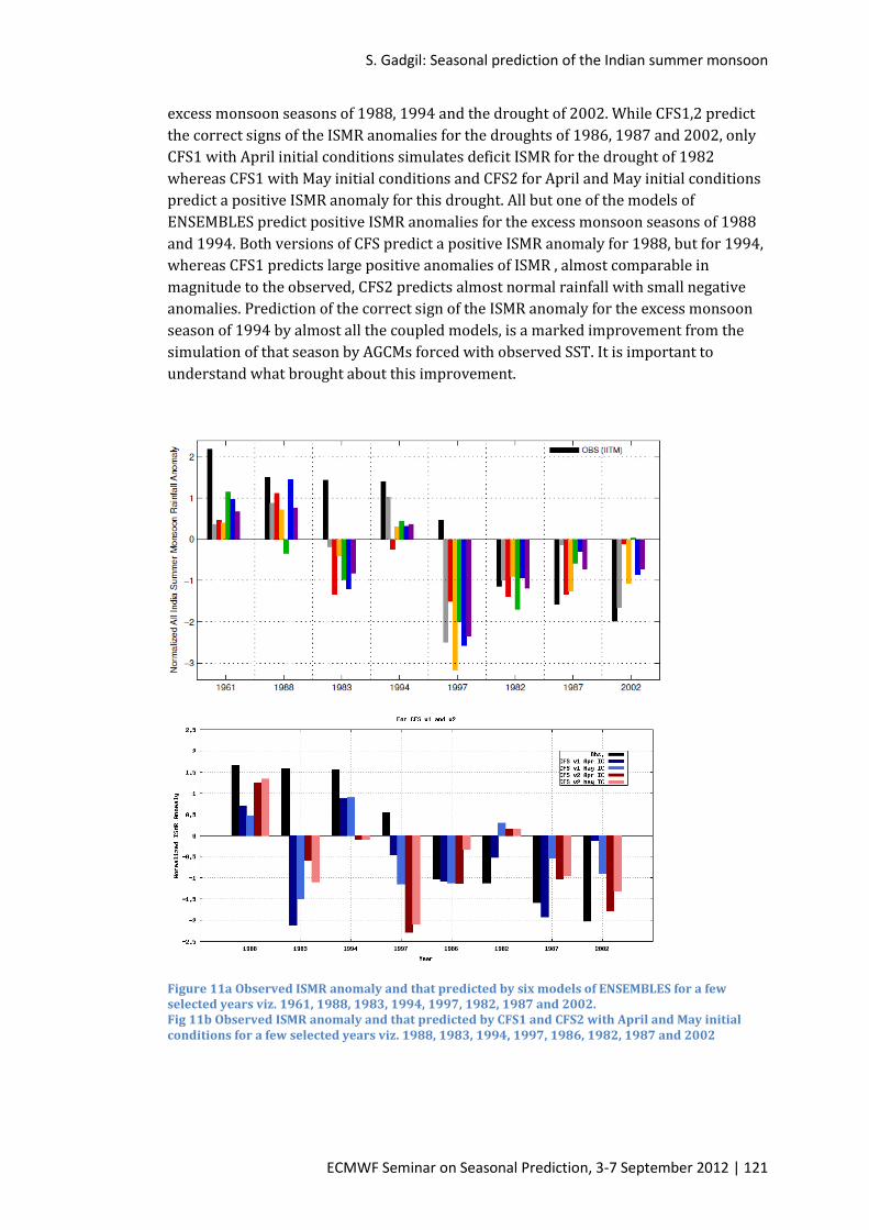
The correlation between the observed and simulated ISMR for the ENSEMBLE models considered by Rajeevan et al (2012), ranges from 0.34 to 0.39 (Table 2 in Rajeevan et al (2012)).The observed ISMR and that simulated by five models, for a few extremes and the special season of 1997 identified by Wang et al. (2004), are shown in Fig. 11a and for CFS1 and CFS2 , for April and May initial conditions, are shown in Fig. 11b.It is seen that, all the models of ENSEMBLES predict the observed sign of ISMR anomaly for the excess monsoon of 1961, the droughts of 1982 and 1987 and all but one for the



excess monsoon seasons of 1988, 1994 and the drought of 2002. While CFS1,2 predict the correct signs of the ISMR anomalies for the droughts of 1986, 1987 and 2002, only CFS1 with April initial conditions simulates deficit ISMR for the drought of 1982 whereas CFS1 with May initial conditions and CFS2 for April and May initial conditions predict a positive ISMR anomaly for this drought. All but one of the models of ENSEMBLES predict positive ISMR anomalies for the excess monsoon seasons of 1988 and 1994. Both versions of CFS predict a positive ISMR anomaly for 1988, but for 1994, whereas CFS1 predicts large positive anomalies of ISMR , almost comparable in magnitude to the observed, CFS2 predicts almost normal rainfall with small negative anomalies. Prediction of the correct sign of the ISMR anomaly for the excess monsoon season of 1994 by almost all the coupled models, is a marked improvement from the simulation of that season by AGCMs forced with observed SST. It is important to understand what brought about this improvement.

Figure 11a Observed ISMR anomaly and that predicted by six models of ENSEMBLES for a few selected years viz. 1961, 1988, 1983, 1994, 1997, 1982, 1987 and 2002. Fig 11b Observed ISMR anomaly and that predicted by CFS1 and CFS2 with April and May initial conditions for a few selected years viz. 1988, 1983, 1994, 1997, 1986, 1982, 1987 and 2002



The most striking feature of Figs 11a and b is the failure of all the five models of ENSEMBLES and the two versions of CFS , with April and May initial conditions, to predict the correct sign of the ISMR anomalies for 1997 and 1983. Instead of the normal monsoon of 1997 (with a small positive ISMR anomaly) and the excess monsoon of 1983, all the models predict large deficits and several of them droughts, implying loud false alarms for these seasons. Thus the difficulties encountered by AGCMs in simulating the ISMR for the El Nino season of 1997 (Wang et al 2004) seem to persist for the coupled models as well. We find that the correlations improve substantially if these years are dropped (Table 2). Clearly, we need to understand why the errors are large for these years even if the aim is only to improve the overall correlation.

Table 2: Correlation between predicted and observed ISMR

Model Period Corr. coeff. Period Corr. coeff. ENSEMBLES MME 1960-2005 0.48 1960-2005

(without 1983,1997) 0.64

CFS2 (April initial cond.)

1982-2009 0.38 1982-2009 (without 1983,1997)

0.57

CFS2 (May initial cond.)

0.32 0.53

Such a coherence in the model predictions for the special seasons of 1997 and 1983 (false alarms), despite the differences in parameterizations etc., can arise from failure/success to predict a critical phenomenon across the board. Rajeevan et al. 2012 have shown that in 1997, the MME of ENSEMBLES, predicted a much stronger El Nino over the central Pacific (which is expected to have a larger negative impact on the Indian monsoon) and did not predict the positive IOD event (which had a large positive impact on the Indian monsoon). In the season of 1983, the warm SST anomalies over the central Pacific were predicted to persist throughout the season, whereas they disappeared half way through the season. Thus the failure of the predictions in 1997 and 1983 have been attributed to the failure in accurate prediction of the spatial pattern and intensity of the anomalies associated with the El Nino of 1997 and of the retreat of the El Nino of 1982-83 from the central Pacific. Gadgil and Francis’s (2013) analysis of the predictions of individual models of ENSEMBLES has shown that for the season of 1997, in most of the models of ENSEMBLES, the region of warm SST anomalies extended westward of the observed across the dateline (as for the MME). However, the pattern of the SST anomalies over the equatorial Indian Ocean varied from model to model. For the Meteo-France model, the anomaly pattern is realistic but the magnitudes smaller than observed; for ECMWF and HadGem2 models, the SST anomalies were of opposite sign to the observed –cold over the WEIO and warm over EEIO (Fig. 12a) while they are positive over almost the entire equatorial Indian Ocean for the other two models. CFS1 and CFS2 predicted that cold SST anomalies over EEIO, as observed, but the magnitude of the anomalies over the western and eastern equatorial Indian Ocean was much smaller than observed (Fig. 12b). It is, thus, important to understand why the IOD event of 1997 was not triggered in most of these models.



Figure 12a For June-September 1997: SST anomalies observed (top) and predicted by HadGem and ECMWF models of ENSEMBLES (middle and bottom).



Fig. 12b For June-September 1997: SST anomalies observed (top) and predicted by CFS1 and CFS2 models of NCEP (middle and bottom)

Consider next the IOD event of 1994. We find that the El Nino signal is much weaker than observed in all the models (Fig. 13a,b). On the other hand, the patterns of the SST as well rainfall anomalies over the equatorial Indian Ocean are well predicted by all the models, although the magnitude is generally smaller (except for CFS1) and almost all predict a positive ISMR anomaly, as observed. A realistic pattern of the SST anomalies over the Pacific, but with a smaller magnitude than observed, is a scenario we considered in the experiment under SPIM in which AGCMS were forced with SST derived by assuming that April persist. Thus the positive ISMR anomaly predicted by most of the coupled models is consistent with the positive ISMR anomalies simulated by the AGCMs in that case. We must, therefore, conclude that the accurate prediction of the sign of the ISMR anomaly for 1994 was possible because of an error involving a



Figure 13a For June-September 1994: SST anomalies observed (top) and predicted by HadGem and ECMWF models of ENSEMBLES (middle and bottom).



Fig. 13b For June-September 1997: SST anomalies observed (top) and predicted by CFS1 and CFS2 models of NCEP (middle and bottom)

smaller magnitude of the El Nino phase than observed. It is necessary to improve the prediction of the El Nino phase in this season and check if the models can still predict the positive ISMR anomaly observed in 1994.



7 Summary and conclusions The impact of seasonal rainfall on agriculture and GDP has been shown to be highly nonlinear with the impact of negative ISMR anomalies much larger than that of positive ISMR anomalies of similar magnitude. A reliable prediction of the non-occurrence of droughts is expected to be very useful in farm level decision making for enhanced agricultural prediction.

The SST-rainfall relationship over Nino 3.4 as well as warm oceans such as the tropical West Pacific, is well simulated by atmospheric and coupled versions of the models of IPCC-AR4. Thus, the poor skill of the AGCMs forced with observed SSTs in simulating the interannual variation of the Indian/Asian monsoon cannot be attributed to the skill in simulation of the SST-rainfall relationship over the warm parts of the tropical Indian-Pacific oceans, and hence to the omission of coupling.

On the whole, the recent coupled models of ENSEMBLES and CFS1,2 of NCEP are able to predict the correct sign of the ISMR anomaly for most of the ISMR extremes. However, almost all fail to do so for the excess monsoon season of 1983 and the strong El Nino season of 1997.

Analysis of these cases suggests that poor skill in prediction of some facets of the two important modes ENSO and EQUINOO leads to the large errors in all the models in some years. It appears that the prediction of the transition from El Nino ( e.g.1983) and the pattern as well as strength of the mature phase (e.g. 1997) needs to be improved. Thus a surprising conclusion is that prediction of some facets of ENSO needs to be improved for better monsoon forecasts.

Analysis of the predictions for 1997 suggests that it is also necessary to improve the simulation of the evolution of EQIUNOO and IOD and, in particular, special attention has to be given to accurate prediction of the triggering of IOD events. It has been proposed that El Nino plays an important role in triggering of an IOD event via suppression of convection over EEIO. It is believed that the IOD event was triggered before the monsoon of 1997 because the transition to El Nino occurred much earlier. Thus, it is intriguing that an IOD event was not predicted by the models in 1997. Whether the transition phase to El Nino was realistically predicted has to be examined. Why the models were able to predict the SST anomaly patterns over IO in 1994, but not in 1997, has to be understood. Clearly, it is also important to predict the impact of the ENSO on EQUINOO and thereby on the Indian monsoon.

Acknowledgements I am grateful to Dr. Franco Molteni for inviting me to give a talk in this interesting seminar. This invitation led to some interesting work on monsoon prediction and consolidation of my ideas on this theme. It is a pleasure to acknowledge valuable inputs from Drs M. Rajeevan, C. K. Unnikrishnan and P A Francis on their work with ENSEMBLES models, Mohit Ved on CFS predictions and discussions with my colleagues Ravi Nanjundiah, J Srinivasan and Arindam Bhattacharya. I would also like to thank Els Kooij-Connally for help, advice and a great deal of patience.



8 References Bony S, Lau KMandSud Y C 1997 Sea surface temperature and large-scale circulation influences on tropical greenhouse effect and cloud radiative forcing. J. Climate 10 2055–2077

Gadgil and Francis 2013 Monsoon prediction with dynamical models: problems and prospects (submitted)

Gadgil Sulochana, and SidharthaGadgil, The Indian Monsoon, GDP and Agriculture, Econ. Pol. Weekly, XLI, 4887-4895, 2006.

Gadgil Sulochana and Sajani S, Monsoon precipitation in the AMIP runs. Climate Dyn. 14, 659–689, 1998

Gadgil, Sulochana and Srinivasan, J., Seasonal prediction of the Indian. Monsoon.Curr. Sci., 100, 343–353, 2011.

Gadgil Sulochana, P. V. Joseph, and N. V. Joshi, Ocean-atmosphere coupling over monsoon regions, Nature, 312 (5990), 141-143, 1984.

Gadgil Sulochana, P. N. Vinayachandran, and P. A. Francis, Droughts of the Indian summer monsoon: Role of clouds over the Indian Ocean, Current science, 85 (12), 1713-1719, 2003.

Gadgil Sulochana, P. N. Vinayachandran, P. A. Francis, and SidharthaGadgil, Extremes of the Indian summer monsoon rainfall, ENSO and equatorial Indian Ocean oscillation, Geophys. Res. Lett., 31 (12), L12,213 1-4, 2004.

Gadgil, Sulochana, Rajeevan, M. and Nanjundiah, R., Monsoon prediction: Why yet another failure? Curr. Sci., 2005, 88, 1389–1400.

Gadgil, Sulochana, P R SeshagiriRao and KNarahariRao.,: Use of Climate Information for Farm-Level Decision Making: Rainfed Groundnut in Southern India, Agricultural Systems, 74, 431-457, 2002

Gadgil Sulochana, M. Rajeevan, and P. A. Francis, Monsoon variability: Links to major oscillations over the equatorial Pacific and Indian oceans, Current science, 93 (2), 182-194, 2007.

Gates W L, AMIP: The atmospheric model intercomparison project. Bull. Amer. Met. Soc. 73, 1962–1970, 1992

Graham N E and Barnett T P Observations of sea surface temperature and convection over tropical oceans. Science 238 657–659, 1987

Ihara, C., Y. Kushnir, M. A. Cane, and V. H. De la Pena, Indian summer monsoon rainfall and its link with ENSO and Indian Ocean climate indices, International Journal of Climatology, 27 (2), 179-187, 2007.

Kang I-S, Jin K, Wang B, Lau K-M, Shukla J, Krishnamurthy V, Schubert S D, Waliser D E , Stern W F, Kitoh A, Meehl G A, Kanamitsu M, Galin V Y, Sathyan V, Park C-K, and Lin Y



Intercomparison of the climatological variation of Asian summer monsoon precipitation simulated by 10 GCMS Clim. Dyn.19 p383–395,2002

Mohit Ved et.al 2013 Monsoons in NCEP model forecasts (submitted)

Nanjundiah, R S, 2009: A Quick Assessment of Forecasts for the Indian Summer Monsoon Rainfall in 2009. CAOS Report No 2009 AS 02

Pant, G. B., and B. Parthasarathy, Some aspects of an association between the southern oscillation and Indian summer monsoon, Arch. Meteorol.Geophys.Biokl,29, 245-251, 1981.

Palmer TN et al ,Development of a European multimodel ensemble system for seasonal to- interannual prediction (DEMETER). Bull Am Meteorol Soc 85:853–872. doi:10.1175/BAMS-85-6-853, 2004

Parthasarathy, B., A. A. Munot, and D. R. Kothawale, Indian summer monsoon rainfall indices: 18711990, Meteorol. Mag., 121, 174-186, 1992.

Parthasarathy, B., A. A. Munot, and D. R. Kothawale, Monthly and seasonal rainfall series for All-India homogeneous regions and meteorological sub-divisions, 1871-1994 pp., Indian Institute of Tropical Meteorology, Pune, INDIA, 1995.

Preethi B, Kripalani RH, Kumar KK (2010) Indian summer monsoon rainfall variability in global coupled ocean-atmospheric models. Clim Dyn 35:1521–1539. doi:10.1007/s00382-009-0657-x

Rajeevan, M., Unnikrishnan, C. K. andPreethi, B., Evaluation of the ENSEMBLES multi-model seasonal forecasts of Indian summer monsoon variability Clim. Dyn, 38, 2257- 2274,DOI:10.1007/s00 382–011–1061–x., 2012

Rajendran K , Ravi S. Nanjundiah, Sulochana Gadgil, and J. Srinivasan,: How good are the simulations of tropical SST-rainfall relationship by IPCC AR4 atmospheric and coupled models? J. Earth System Sciences, 121 (3), 595-610, 2012.

Rasmusson, E. M., and T. H. Carpenter, The relationship between eastern equatorial Pacific sea surface temperatures and rainfall over India and Sri Lanka , Mon. Weather Rev., 111, 517-528, 1983.

Saji, N. H., Goswami, B. N., Vinayachandran, P. N. and Yamagata,T., A dipole mode in the tropical Indian Ocean. Nature, 401, 360–363, 1999.

Sikka, D. R., Some aspects of the large-scale fluctuations of summer monsoon rainfall over India in relation to fluctuations in the planetary and regional scale circulation parameters, Proc. Indian Acad. Sci. (Earth Planet. Sci), 89, 179-195, 1980.

Sivakumar M V K, P Singh ans J S Williams, Agroclimatic aspects in planning for improved productivity in Alfisols pages 15-30 in: Alfisols in the semi-arid tropics: a consultant’s workshop, 1-3 December 1983 ICRISAT Centre, India, 1983.



Sperber K R and Palmer T N,Interannual tropical rainfall variability in general circulation model simulations associated with the Atmospheric Model IntercomparisonProject, J. Climate9 2727–2750, 1996

Waliser D E and Graham N E, Convective cloud system and warm pool sea-surface temperature :coupled interaction and self regulation, J. Geophys. Res. 98 12881–12893, 1993

Wang B, Kang I -S and Lee J -Y Ensemble simulations of Asian-Australian monsoon variability by 11 AGCMs, J. Climate 17 803–818, 2004

Wang B, Ding Q, Fu X, Kang I -S, Jin K, Shukla J and Doblas-Reyes F Fundamental challenge in simulation and prediction of summer monsoon rainfall Geophys. Res. Lett. 32 , 15711doi:10.1029/2005Gl022734, 2005

Webster, P. J., Moore, A. M., Loschnigg, J. P. and Leben, R. R., Coupled ocean–atmosphere dynamics in the Indian Ocean during 1997–1998. Nature, 401, 356–360, 1999.

Zhang C, Large-scale variability of atmospheric deep convection in relation to sea surface temperature in the tropics J. Climate 6 1898–1912, 1993

seasonal prediction of the indian summer monsoon: … seminar on seasonal prediction, 3-7 september...

Documents